Heteroscedasticity in survey Data and model selection based on weighted HQIC
24
Journal of Reliability and Statistical Studies; ISSN (Print): 0974-8024, (Online):2229-5666 Vol. 6, Issue 2 (2013): 17-40 HETEROSCEDASTICITY IN SURVEY DATA AND MODEL SELECTION BASED ON WEIGHTED HANNAN-QUINN INFORMATION CRITERION G.S. David Sam Jayakumar 1 and A.Sulthan 2 Jamal Institute of Management Tiruchirappalli-620020, India Email: 1 [email protected], 2 [email protected] (Received October 12, 2012) Abstract This paper made an attempt on the weighted version of Hannan-Quinn information criterion for the purpose of selecting a best model from various competing models, when heteroscedasticity is present in the survey data. The authors found that the information loss between the true model and fitted models are equally weighted, instead of giving unequal weights. The computation of weights purely depends on the differential entropy of each sample observation and traditional Hannan-Quinn information criterion was penalized by the weight function which comprised of the Inverse variance to mean ratio (VMR) of the fitted log quantiles.The Weighted Hannan-Quinn information criterion was explained in two versions based on the nature of the estimated error variances of the model namely Homogeneous and Heterogeneous WHQIC respectively. The WHQIC visualizes a transition in model selection and it leads to conduct a logical statistical treatment for selecting a best model. Finally, this procedure was numerically illustrated by fitting 12 different types of stepwise regression models based on 44 independent variables in a BSQ (Bank service Quality) study. Key Words: Hannan-Quinn Information Criterion, Weighted Hannan-Quinn Information Criterion, Differential Entropy, Log-Quantiles, Variance To Mean Ratio. 1. Introduction and Related Work Model selection is the task of selecting a statistical model from a set of candidate models, given data. Penalization is an approach to select a model that fits well with data which minimize the sum of empirical risk FPE (Akaike, 1970), AIC (Akaike. 1973), Mallows’ Cp (Mallows, 1973). Many authors studied and proposed about penalties proportion to the dimension of model in regression, showing under various assumption sets that dimensionality-based penalties like Cp are asymptotically optimal (Shibata, 1981, Ker-Chau Li. 1987, Polyak and Tsybakov, 1990) and satisfy non-asymptotic oracle inequalities (Baraud, 2000, Baraud, 2002, Barron, 1999, Birg´e and Massart, 2007). It is assumed that data can be heteroscedastic, but not necessary with certainty (Arlot, 2010). Several estimators adapting to heteroscedasticity have been built thanks to model selection (Gendre, 2008), but always assuming the model collection has a particular form. Past studies show that the general problem of model selection when the data are heteroscedastic can be solved only by cross-validation or resampling based procedures. This fact was recently confirmed, since resampling and V-fold penalties satisfy oracle inequalities for regressogram selection when data are heteroscedastic (Arlot 2009), there is a significant increase of the computational complexity by adapting heteroscedasticity with resampling. Inliers detection using Schwartz information criterion by illustrated with a simulated experiment and a real life
Transcript of Heteroscedasticity in survey Data and model selection based on weighted HQIC
Journal of Reliability and Statistical Studies; ISSN (Print): 0974-8024, (Online):2229-5666
Vol. 6, Issue 2 (2013): 17-40
HETEROSCEDASTICITY IN SURVEY DATA AND MODEL
SELECTION BASED ON WEIGHTED HANNAN-QUINN
INFORMATION CRITERION
G.S. David Sam Jayakumar1 and A.Sulthan
2
Jamal Institute of Management
Tiruchirappalli-620020, India
Email: [email protected],
(Received October 12, 2012)
Abstract
This paper made an attempt on the weighted version of Hannan-Quinn information
criterion for the purpose of selecting a best model from various competing models, when
heteroscedasticity is present in the survey data. The authors found that the information loss
between the true model and fitted models are equally weighted, instead of giving unequal
weights. The computation of weights purely depends on the differential entropy of each sample
observation and traditional Hannan-Quinn information criterion was penalized by the weight
function which comprised of the Inverse variance to mean ratio (VMR) of the fitted log
quantiles.The Weighted Hannan-Quinn information criterion was explained in two versions based
on the nature of the estimated error variances of the model namely Homogeneous and
Heterogeneous WHQIC respectively. The WHQIC visualizes a transition in model selection and
it leads to conduct a logical statistical treatment for selecting a best model. Finally, this procedure
was numerically illustrated by fitting 12 different types of stepwise regression models based on
44 independent variables in a BSQ (Bank service Quality) study.
Key Words: Hannan-Quinn Information Criterion, Weighted Hannan-Quinn Information
Criterion, Differential Entropy, Log-Quantiles, Variance To Mean Ratio.
1. Introduction and Related Work Model selection is the task of selecting a statistical model from a set of
candidate models, given data. Penalization is an approach to select a model that fits
well with data which minimize the sum of empirical risk FPE (Akaike, 1970), AIC
(Akaike. 1973), Mallows’ Cp (Mallows, 1973). Many authors studied and proposed
about penalties proportion to the dimension of model in regression, showing under
various assumption sets that dimensionality-based penalties like Cp are asymptotically
optimal (Shibata, 1981, Ker-Chau Li. 1987, Polyak and Tsybakov, 1990) and satisfy
non-asymptotic oracle inequalities (Baraud, 2000, Baraud, 2002, Barron, 1999, Birg´e
and Massart, 2007). It is assumed that data can be heteroscedastic, but not necessary
with certainty (Arlot, 2010). Several estimators adapting to heteroscedasticity have
been built thanks to model selection (Gendre, 2008), but always assuming the model
collection has a particular form. Past studies show that the general problem of model
selection when the data are heteroscedastic can be solved only by cross-validation or
resampling based procedures. This fact was recently confirmed, since resampling and
V-fold penalties satisfy oracle inequalities for regressogram selection when data are
heteroscedastic (Arlot 2009), there is a significant increase of the computational
complexity by adapting heteroscedasticity with resampling. Inliers detection using
Schwartz information criterion by illustrated with a simulated experiment and a real life

18 Journal of Reliability and Statistical Studies, Dec. 2013, Vol. 6(2)
data. (Muralidharan and Kale Nevertheless, 2008). The main goal of the paper is to
propose a WHQIC (Weighted Hannan-Quinn information criterion) if the problem of
heteroscedasticity is present in the survey data. The derivation procedures of WHQIC
and different versions of the criteria are discussed in the subsequent sections.
2. Homogeneous Weighted Hannan-Quinn Information Criterion This section deals with the presentation of the proposed Weighted Hannan-
Quinn information criterion. At first the authors highlighted the Hannan-Quinn
information criterion of a model based on log likelihood function and the blend of
information theory is given as
2log ( / ) 2 log(log )HQIC L X k nθ=− +ɵ … (1)
where θɵ is the estimated parameter, X is the data matrix, ( / )L Xθɵ is the maximized
likelihood function and 2 log(log )k n is the penalty function which comprised of
sample size (n) and no. of parameters (k) estimated in the fitted model. From (1), the
shape of HQIC changes according to the nature of the penalty functions. Similarly, we
derived a Weighted Hannan-Quinn Information Criterion (WHQIC) based on the HQIC
of a given model. Rewrite (1) as
1
2log( ( / )) 2 log(log )n
i
i
HQIC f x k nθ=
=− +∏ ɵ
1
2 log( ( / )) 2 log(log )n
i
i
HQIC f x k nθ=
=− +∑ ɵ
1
( 2 log ( / ) (2 log(log ) / ))n
i
i
HQIC f x k n nθ=
= − +∑ ɵ … (2)
From (2), the quantity 2log ( / ) (2 log(log ) / )if x k n nθ− +ɵ is the unweighted
point wise information loss of an ith
observation for a fitted model. The proposed
WHQIC assured each point wise information loss should be weighted and it is defined
as
1
( 2 log ( / ) (2 log(log ) / ))n
i i
i
WHQIC w f x k n nθ=
= − +∑ ɵ … (3)
From (3), the weight of the point wise information loss shows the importance of the
weightage that the model selector should give at the time of selecting a particular
model. Here the problem is how the weights are determined? The authors found, there
is a link between the log quantiles of a fitted density function and the differential
entropy. The following shows the procedure of deriving the weights.
Take mathematical expectation for (3), we get the expected WHQIC as
1
( ) (2 ( log ( / )) (2 log(log ) / ))n
i i
i
E WHQIC w E f x k n nθ=
= − +∑ ɵ … (4)

Heteroscedasticity in Survey Data and Model Selection Based on … 19
where the term ( log ( / )) log ( / ) ( / )i i i i
d
E f x f x f x dxθ θ θ− = −∫ɵ ɵ ɵ is the
differential entropy of the ith
observation and d is the domain of ix , which is also
referred as expected information in information theory. Now from (3) and (4), the
variance of the WHQIC is given as
2
1
( ) 4 ( ( log ( / ) ( log ( / ))))n
i i i
i
V WHQIC E w f x E f xθ θ=
= − − −∑ ɵ ɵ
2
1 1 1
( ) 4( ( log ( / )) 2 ((( log ( / ) ( log ( / ))(( log ( / ) ( log ( / ))))n n n
i i i j i i j j
i i j
V WHQIC w V f x wwE f x E f x f x E f xθ θ θ θ θ= = =
= − − − − − − − −∑ ∑∑ɵ ɵ ɵ ɵ ɵ
… (5)
From (5) i j≠ , the variance of the WHQIC was reduced by using iid property of the
sample observation and it is given as
2
1
( ) 4( ( log ( / )))n
i i
i
V WHQIC w V f x θ=
= −∑ ɵ … (6)
where
2( log ( / )) ( log ( / ) ( log ( / ))) ( / )i i i i i
d
V f x E f x E f x f x dxθ θ θ θ− = − − −∫ɵ ɵ ɵ ɵ
is the variance of the fitted log quantiles which explains the variation between the
actual and the expected point wise information loss. In order to determine the weights,
the authors wants to maximize ( )E WHQIC and minimize ( )V WHQIC , because if
the expected weighted information loss is maximum, then the variation between the
actual weighted information and its expectation will be minimum. For this, maximize
the difference (D) between the ( )E WHQIC and ( )V WHQIC which simultaneously
optimize ( )E WHQIC and ( )V WHQIC then the D is given as
( ) ( )D E WHQIC V WHQIC= − … (7)
2
1 1
(2 ( log ( / )) (2 log(log ) / )) 4( ( log ( / )))n n
i i i i
i i
D w E f x k n n w V f xθ θ= =
= − + − −∑ ∑ɵ ɵ
Using classical unconstrained optimization technique, maximize D with respect to the
weights (w) by satisfying the necessary and sufficient conditions such as 0i
D
w
∂=
∂ ,
2
20
i
D
w
∂<
∂ and it is given as
2 ( log ( / ) 8 ( log ( / )) 0i i i
i
DE f x w V f x
wθ θ
∂= − − − =
∂ɵ ɵ ... (8)

20 Journal of Reliability and Statistical Studies, Dec. 2013, Vol. 6(2)
2
28 ( log ( / )) 0i
i
DV f x
wθ
∂=− − <
∂ɵ … (9)
By solving (8), we get the unconstrained weights as
( log ( / )
4 ( log ( / ))
ii
i
E f xw
V f x
θ
θ
−=
−
ɵ
ɵ … (10)
From (8) and (9), it is impossible to use the second derivative Hessian test to find the
absolute maximum or global maximum of the function D with respect to iw ,because
the cross partial derivative 2 / i jD w w∂ ∂ ∂ is 0 and iw is not existing in
2 2/ iD w∂ ∂.Hence the function D achieved the local maximum or relative maximum at the point
iw .Then from (10) rewrite the expectation and variance in terms of the integral
representation as
2
log ( / ) ( / )
4 ( log ( / ) ( log ( / ))) ( / )
i i i
di
i i i i
d
f x f x dx
wE f x E f x f x dx
θ θ
θ θ θ
−
=− − −
∫
∫
ɵ ɵ
ɵ ɵ ɵ
The equation (10), can also be represented in terms of VMR of fitted log quantiles and
it is given as
1
4 ( log ( / ))i
i
wVMR f x θ
=− ɵ
… (11)
where ( log ( / ))
( log ( / ))( log ( / ))
ii
i
V f xVMR f x
E f x
θθ
θ
−− =
−
ɵɵ
ɵ is the variance to mean ratio.
From (10) and (11), the maximum likelihood estimate θɵ is same for all sample
observations and the entropy, variance of the fitted log-quantiles are same for all i.
Then iw w= , then (3) becomes
1
( 2 log ( / ) (2 log(log ) / ))n
i
i
WHQIC w f x k n nθ=
= − +∑ ɵ … (12)
where ( log ( / ))
4 ( log ( / ))
E f xw
V f x
θ
θ
−=
−
ɵ
ɵ for all i and substitute in (12), we get the
homogeneous weighted version of the Weighted Hannan-Quinn information criterion as
1
( log ( / ))( ) ( 2 log ( / ) (2 log(log ) / ))4 ( log ( / ))
n
i
i
E f xWHQIC f x k n n
V f x
θθ
θ =
−= − +
−∑
ɵɵ
ɵ

Heteroscedasticity in Survey Data and Model Selection Based on … 21
1
( 2 log ( / ) (2 log(log ) / ))
4 ( log ( / ))
n
i
i
f x k n n
WHQICVMR f x
θ
θ
=
− +=
−
∑ ɵ
ɵ … (13)
Combining (1) and (13) we get the final version of the homogeneous Weighted
Hannan-Quinn information criterion as
4 ( log ( / ))
HQICWHQIC
VMR f x θ=
− ɵ … (13a)
If a sample normal linear regression model is evaluated, with a single dependent
variable ( Y ) with p regressors namely 1 2 3, , ,...
i i i piX X X X in matrix notation is
given as
Y X eβ= + … (13b)
where ( 1)nXY is the matrix of the dependent variable,
( 1)kX
β is the matrix of beta co-
efficients or partial regression co-efficients and ( 1)nXe is the residual followed normal
distribution N (0,2
e nIσ ).From (13a), the sample regression model should satisfy the
assumptions of normality, homoscedasticity of the error variance and the serial
independence property. Then the WHQIC of a fitted linear regression model is given as
��24 ( log ( / , , ))e
HQICWHQIC
VMR f Y X β σ=
− … (14)
where �β ,�2
eσ are the maximum-likelihood estimates
� �22log ( , / , ) 2 log(log( ))e
HQIC L Y X k nβ σ=− + , ��2( log ( / , , ))eVMR f Y X β σ−
is the variance to mean ratio of the fitted normal log quantiles and k is the no.of
parameters estimated in the model (includes the Intercept and estimated error variance).
From (14) VMR can be evaluated as
����
��
22
2
( log ( / , , ))( log ( / , , ))
( log ( / , , ))
ee
e
V f Y XVMR f Y X
E f Y X
β σβ σ
β σ
−− =
− … (15)
� �
� � � � � �
� � � �
2 2 2 2
2
2 2
( log ( / , , ) ( log ( / , , ))) ( / , , )
( log ( / , , ))
log ( / , , ) ( / , , )
e e e
e
e e
E f Y X E f Y X f Y X dY
VMR f Y X
f Y X f Y X dY
βσ βσ β σ
βσ
β σ β σ
+∞
−∞+∞
−∞
− − −
− =
−
∫
∫

22 Journal of Reliability and Statistical Studies, Dec. 2013, Vol. 6(2)
Where � �
�
�
� 2
2
1( )
22
2
1( / , , ) ,
2
e
Y X
e
e
f Y X e Y
β
σβ σ
πσ
− −
= −∞< <+∞ is the fitted
normal density function and the expectation and variance of the quantity
� �2log ( / , , )ef Y X β σ− is given as
� � � � � � �2 2 2 21( log ( / , , )) ( log ( / , , )) ( / , , ) (1 log(2 ))
2e e e eE f Y X f Y X f Y X dyβσ βσ βσ πσ
+∞
−∞
− = − = +∫
... (16)
� � � � � � � �2 2 2 2 2 1( log ( / , , )) ( log ( / , , ) ( log ( / , , )) ( / , , )
2e e e eV f Y X E f Y X E f Y X f Y X dyβ σ β σ β σ β σ
+∞
−∞
− = − − − =∫ … (17)
Substitute (16) and (17) in (15), then we get VMR for the fitted Normal log quantiles as
� �
�
2
2
1( log ( / , , ))
(1 log(2 ))e
e
VMR f Y X β σπσ
− =+
… (18)
Substitute (18) in (14), we get
�2(1 log(2 ))
4
eWHQIC HQICπσ+
= … (19)
Where �21
(1 log(2 ))4
ew πσ= + … (20)
From (19), WHQIC is the product of the weight and the traditional Hannan-Quinn
information criterion. The WHQIC incorporates the dispersion in the fitted normal log
quantiles and weighs the point wise information loss equally, but not with the unit
weights. The mono weighted Hannan-Quinn information criterion works based on the
assumption of the homoscedastic error variance. If it is heteroscedastic, then we get the
variable weights and the procedures are discussed in the next section.
3. Heterogeneous Weighted Akaike Information Criterion The homogeneous weighted Hannan-Quinn information criterion is
impractical due to the assumption of homoscedasticity of the error variance. If this
assumption is violated, then the weights vary for each point wise information loss, but
the estimation of heteroscedastic error variance based on maximum likelihood
estimation is difficult (cordeiro (2008), Fisher (1957)). For this, the authors utilize the
link between the maximum likelihood theory and Least squares estimation to estimate
the heteroscedastic error variance based on the linear regression model.
Let the random error of the linear regression model can be given as
( )e I H Y= − … (21)
From (21), the random errors are the product of actual value of Y and the residual
operator ( )I H− where H is the Hat matrix. Myers, Montgomery (1997) proved the
magical properties of the residual operator matrix as idempotent and symmetric. Based
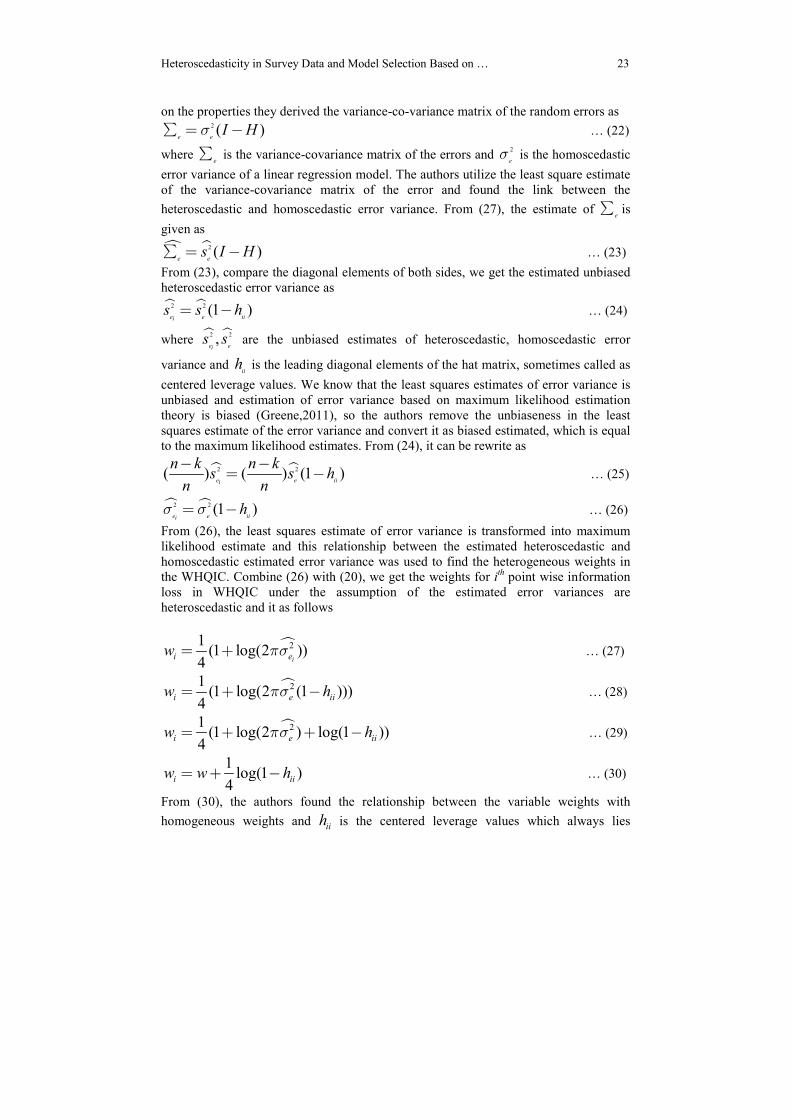
Heteroscedasticity in Survey Data and Model Selection Based on … 23
on the properties they derived the variance-co-variance matrix of the random errors as 2 ( )
e eI Hσ∑ = − … (22)
where e∑ is the variance-covariance matrix of the errors and
2
eσ is the homoscedastic
error variance of a linear regression model. The authors utilize the least square estimate
of the variance-covariance matrix of the error and found the link between the
heteroscedastic and homoscedastic error variance. From (27), the estimate of e∑ is
given as
� �2 ( )e e
s I H∑ = − … (23)
From (23), compare the diagonal elements of both sides, we get the estimated unbiased
heteroscedastic error variance as
� �2 2 (1 )e e iii
s s h= − … (24)
where � �2 2,e ei
s s are the unbiased estimates of heteroscedastic, homoscedastic error
variance and ii
h is the leading diagonal elements of the hat matrix, sometimes called as
centered leverage values. We know that the least squares estimates of error variance is
unbiased and estimation of error variance based on maximum likelihood estimation
theory is biased (Greene,2011), so the authors remove the unbiaseness in the least
squares estimate of the error variance and convert it as biased estimated, which is equal
to the maximum likelihood estimates. From (24), it can be rewrite as
� �2 2( ) ( ) (1 )e e iii
n k n ks s h
n n
− −= − … (25)
� �2 2 (1 )e e iii
hσ σ= − … (26)
From (26), the least squares estimate of error variance is transformed into maximum
likelihood estimate and this relationship between the estimated heteroscedastic and
homoscedastic estimated error variance was used to find the heterogeneous weights in
the WHQIC. Combine (26) with (20), we get the weights for ith
point wise information
loss in WHQIC under the assumption of the estimated error variances are
heteroscedastic and it as follows
�21(1 log(2 ))
4 ii ew πσ= + … (27)
�21(1 log(2 (1 )))
4i e iiw hπσ= + − … (28)
�21(1 log(2 ) log(1 ))
4i e iiw hπσ= + + − … (29)
1log(1 )
4i iiw w h= + − … (30)
From (30), the authors found the relationship between the variable weights with
homogeneous weights and ii
h is the centered leverage values which always lies
24 Journal of Reliability and Statistical Studies, Dec. 2013, Vol. 6(2)
between the / 1ii
p n h≤ ≤ ,where p is the no.of regressors. Hence, the authors proved
from (29),if the estimated error variance is homoscedastic, we can derive the
heteroscedastic error variance based on the hat values. Moreover, the variable weights
gave importance to the point wise information loss unequally which the WHQIC can be
derived by combining (3) and (29) in terms of the linear regression model as
� � �2 21((1 log(2 (1 )))( 2log ( / , , ) (2 log(log )/ )))
4e ii e
i
WHQIC h f Y X k n nπσ β σ= + − − +∑
…(31)
4. Results and Discussion In this section, we will investigate the discrimination between the traditional
HQIC and the proposed WHQIC on the survey data collected from BSQ (Bank Service
Quality) study. The data comprised of 45 different attributes about the Bank and the
data was collected from 102 account holders. A well-structured questionnaire was
prepared and distributed to 125 customers and the questions were anchored at five point
Likert scale from 1 to 5. After the data collection is over, only 102 completed
questionnaires were used for analysis. The following table shows the results extracted
from the analysis by using SPSS version 20. At first, the authors used, stepwise
multiple regression analysis by utilizing 44 independent variables and a dependent
variable. The results of the stepwise regression analysis with model selection criteria
are visualized in the following Table 1 with results of subsequent analysis.

Heteroscedasticity in Survey Data and Model Selection Based on … 25
Table 1: Stepwise Regression Summary, Traditional HQIC and Weighted HQIC
Model Regression summary
Homogeneous
Weighted HQIC
K EHEV R2 F-ratio UWHQIC MAX(D) E(WHQIC)
1 3 0.230 0.188 23.089* 147.962 27.15 51.15
2 4 0.190 .331 24.485* 131.221 21.24 38.87
3 5 0.177 .377 19.753* 127.038 19.76 35.30
4 6 0.167 .410 16.842* 124.547 18.95 33.06
5 7 0.164 .441 15.135* 125.638 19.11 32.69
6 8 0.157 .489 15.140* 123.920 18.38 30.72
7 9 0.147 .525 14.814* 121.944 17.26 28.14
8 10 0.141 .565 15.083* 121.814 16.62 26.49
9 11 0.133 .598 15.188* 120.102 15.60 24.26
10 12 0.126 .615 14.542* 118.262 14.46 21.91
11 13 0.123 .634 14.182* 120.426 14.46 21.52
12 12 0.127 .630 15.466* 119.996 14.81 22.49
Model
Homogeneous Weighted
HQIC Heterogeneous Weighted HQIC
V(WHQIC) W WHQIC MAX(D) E(WHQIC) V(WHQIC) WHQIC
1 24.00 0.343 50.751 26.738 50.350 23.612 50.239
2 17.64 0.294 38.579 20.603 37.663 17.060 37.843
3 15.54 0.276 35.062 18.870 33.623 14.753 33.914
4 14.11 0.263 32.756 17.678 30.712 13.034 31.275
5 13.58 0.258 32.415 17.541 29.824 12.283 30.606
6 12.34 0.246 30.484 16.514 27.378 10.864 28.163
7 10.88 0.231 28.169 15.105 24.350 9.245 25.480
8 9.87 0.220 26.799 14.215 22.333 8.118 23.552
9 8.66 0.206 24.741 12.937 19.740 6.803 21.285
10 7.45 0.191 22.588 11.650 17.241 5.591 18.959
11 7.06 0.186 22.399 11.312 16.381 5.069 18.100
12 7.68 0.194 23.279 11.930 17.704 5.774 19.350
*P-value <0.01 HQIC- Hannan Quinn Information Criterion
EHEV-Estimated homoscedastic error variance MAX (D)-Maximized difference
W-Weights E(WHQIC)-Expectation of weighted Hannan Quinn information criteria
V (WHQIC)-Variance of Hannan Quinn information criteria

26 Journal of Reliability and Statistical Studies, Dec. 2013, Vol. 6(2)
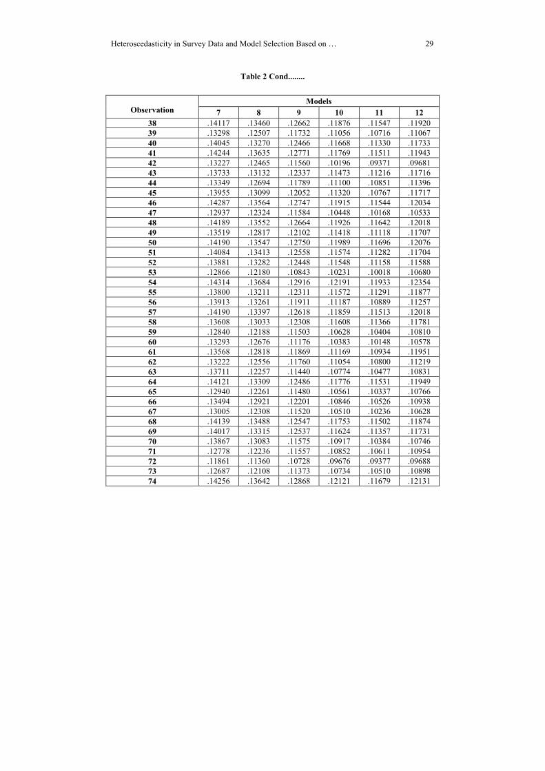
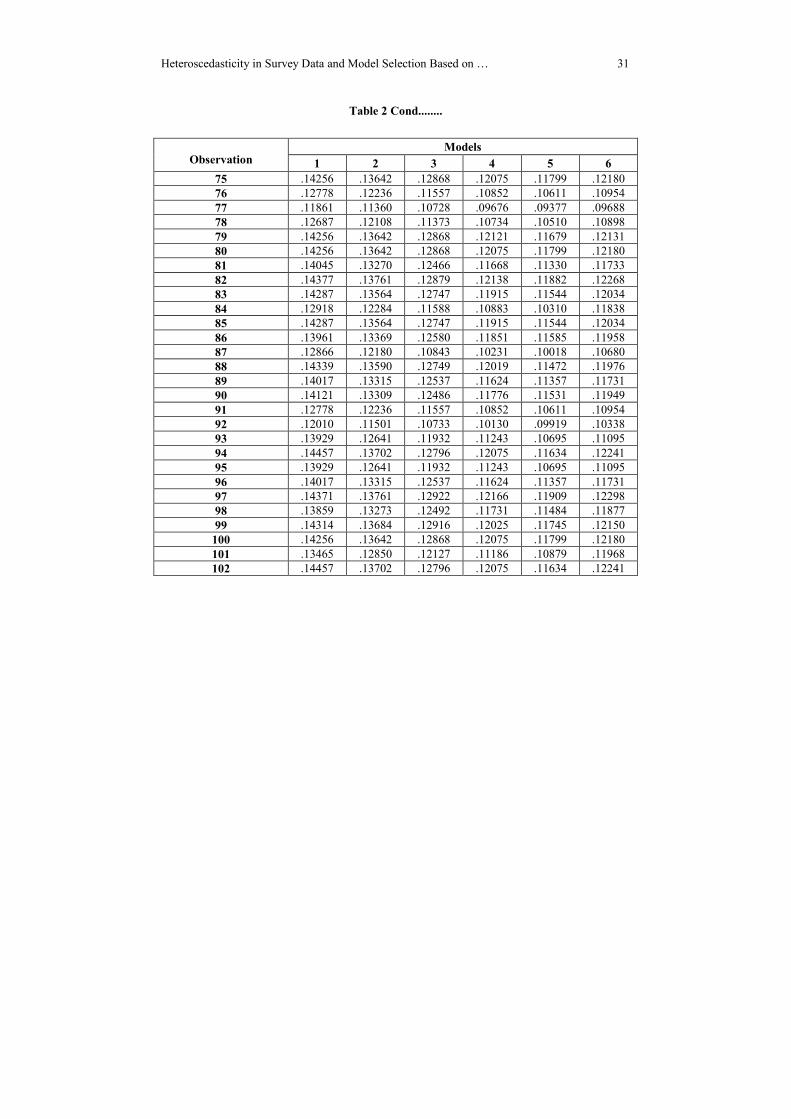
Table 2-Estimated Heteroscedastic Error Variance of Models
Observation Models
1 2 3 4 5 6
1 .22981 .18738 .17348 .16360 .16046 .15234
2 .22981 .18738 .17348 .16264 .15952 .15095
3 .22467 .18347 .16254 .15310 .14459 .13776
4 .22991 .18859 .17448 .16416 .16014 .15206
5 .22991 .17892 .16491 .15443 .15038 .14309
6 .22981 .18827 .17475 .16448 .15937 .15076
7 .22497 .18471 .17095 .16045 .15718 .14937
8 .22981 .18738 .17375 .16419 .15932 .15061
9 .22497 .18265 .16946 .15964 .15648 .14510
10 .22467 .18347 .16991 .15881 .15544 .14802
11 .22981 .18827 .16815 .15095 .14775 .13967
12 .22981 .18738 .17375 .16419 .15257 .14322
13 .22991 .18710 .17316 .16299 .15866 .15012
14 .22991 .18859 .17448 .16416 .16058 .15289
15 .22991 .18859 .17448 .16416 .16014 .15206
16 .22981 .18738 .16598 .15603 .15129 .14400
17 .22991 .18710 .17316 .16299 .15866 .15012
18 .22991 .18710 .17356 .16379 .15504 .14768
19 .21449 .17511 .16169 .15283 .14924 .14179
20 .22991 .18859 .17448 .16416 .15591 .14859
21 .22991 .18859 .17448 .16416 .16058 .15289
22 .22991 .18859 .16825 .15898 .15593 .14812
23 .22981 .18827 .17412 .16412 .15786 .14860
24 .22991 .18710 .16553 .15522 .14895 .14184
25 .22991 .17892 .16631 .15719 .15415 .14674
26 .22991 .18859 .17498 .16501 .16176 .15371
27 .22981 .18827 .17412 .16412 .16095 .15317
28 .21449 .17538 .16245 .15377 .15003 .12835
29 .22991 .18710 .17356 .16250 .15856 .15107
30 .22981 .18738 .17375 .16419 .16097 .15286
31 .22991 .18859 .17498 .16501 .15826 .14949
32 .22991 .18859 .17448 .16416 .16014 .15206
33 .22991 .18859 .17498 .16501 .16176 .15371
34 .22991 .18859 .17498 .15697 .15203 .13543
35 .22991 .18859 .16825 .15898 .15345 .14609
36 .22991 .18710 .17316 .16272 .15944 .15107
37 .22467 .18378 .17062 .16067 .15723 .14910

Heteroscedasticity in Survey Data and Model Selection Based on … 27
Table 2 Contd........
Observation Models
7 8 9 10 11 12
1 .13420 .12727 .12003 .11297 .11057 .11440
2 .14135 .13423 .12679 .11951 .11619 .11999
3 .12918 .12284 .11588 .10883 .10310 .11838
4 .14199 .13398 .12649 .11934 .11642 .12042
5 .13262 .12685 .11981 .10881 .10433 .10867
6 .14175 .13454 .12645 .11899 .11584 .11960
7 .13993 .13398 .12651 .11895 .11600 .11975
8 .14165 .13550 .12730 .11667 .10840 .11422
9 .13494 .12921 .12201 .10846 .10526 .10938
10 .13835 .13149 .12021 .11230 .10886 .11352
11 .13111 .12133 .11155 .10502 .10226 .10728
12 .13462 .12866 .12089 .11374 .09768 .10472
13 .14114 .13491 .12725 .11929 .11556 .12110
14 .14302 .13363 .12348 .11477 .11233 .11735
15 .14199 .13560 .12798 .11227 .10986 .11365
16 .13465 .12850 .12127 .11186 .10879 .11968
17 .14114 .13491 .10853 .09876 .09664 .09976
18 .13877 .13290 .12481 .11716 .11467 .11872
19 .13291 .12687 .11879 .11209 .10862 .11217
20 .13857 .13271 .12276 .11450 .11205 .11733
21 .14302 .13693 .12686 .11807 .11513 .11953
22 .13929 .12641 .11932 .11243 .10695 .11095
23 .13826 .13240 .12494 .11719 .11446 .11835
24 .13248 .12661 .11523 .10828 .10444 .11322
25 .13766 .13125 .12357 .11483 .10908 .11433
26 .14457 .13702 .12796 .12075 .11634 .12241
27 .14340 .13721 .12925 .12171 .11860 .12244
28 .12010 .11501 .10733 .10130 .09919 .10338
29 .14176 .10486 .09848 .09258 .08888 .09195
30 .14377 .13761 .12879 .12138 .11882 .12268
31 .13660 .13038 .12231 .11541 .11215 .11577
32 .14256 .13642 .12868 .12121 .11679 .12131
33 .14205 .13523 .12603 .11840 .11389 .12076
34 .12014 .11114 .10450 .09726 .09516 .09835
35 .13737 .12947 .11960 .11183 .09419 .09838
36 .14140 .13416 .12666 .11678 .11337 .11703
37 .14004 .13288 .12465 .11757 .11474 .11844

28 Journal of Reliability and Statistical Studies, Dec. 2013, Vol. 6(2)
Table 2 Cond........
Observation Models
1 2 3 4 5 6
38 .22991 .18859 .17448 .16407 .15988 .15134
39 .21449 .17511 .16169 .15283 .14929 .14219
40 .22991 .18710 .17356 .16250 .15856 .14947
41 .22991 .18710 .17356 .16379 .15998 .15143
42 .22467 .18347 .16991 .16046 .15007 .14124
43 .22991 .18710 .17356 .16250 .15418 .14665
44 .22467 .18378 .16985 .16035 .15717 .14947
45 .22981 .18827 .17412 .16412 .15786 .14860
46 .22981 .18827 .17412 .16334 .16021 .15213
47 .22991 .18859 .17498 .16407 .14813 .14106
48 .22981 .18738 .17375 .16221 .15907 .15139
49 .22991 .17892 .16491 .15554 .15234 .14401
50 .22991 .18859 .17448 .16407 .16060 .15264
51 .22991 .18710 .17356 .16250 .15856 .15107
52 .22991 .18859 .17498 .16407 .15700 .14963
53 .22991 .18710 .17356 .15224 .14452 .13708
54 .22991 .18859 .17448 .16416 .16058 .15289
55 .22497 .18265 .16894 .15864 .15462 .14703
56 .22991 .18710 .17316 .16299 .15866 .15012
57 .22991 .18859 .17448 .16407 .16060 .15264
58 .22991 .18859 .17448 .16416 .15591 .14647
59 .22981 .18738 .17375 .15126 .14547 .13782
60 .22497 .18471 .16446 .15290 .14962 .14133
61 .22991 .18859 .16825 .15702 .15400 .14658
62 .22981 .18827 .17412 .16334 .15053 .14128
63 .22981 .18738 .17375 .16221 .15713 .14786
64 .22981 .18738 .17375 .16419 .16097 .15286
65 .22467 .18347 .17005 .16085 .15586 .14832
66 .22497 .18265 .16946 .15964 .15648 .14510
67 .22497 .18265 .16894 .15864 .15462 .14703
68 .22981 .18738 .17375 .16221 .15907 .15058
69 .22467 .18378 .17062 .16067 .15723 .14949
70 .22467 .18378 .17062 .16067 .15723 .14910
71 .22497 .18265 .16946 .15964 .15287 .13608
72 .22991 .17892 .16631 .15719 .15415 .14579
73 .22991 .18859 .17498 .15697 .15203 .13543
74 .22991 .18859 .17448 .16416 .16014 .15206
Heteroscedasticity in Survey Data and Model Selection Based on … 29
Table 2 Cond........
Observation Models
7 8 9 10 11 12
38 .14117 .13460 .12662 .11876 .11547 .11920
39 .13298 .12507 .11732 .11056 .10716 .11067
40 .14045 .13270 .12466 .11668 .11330 .11733
41 .14244 .13635 .12771 .11769 .11511 .11943
42 .13227 .12465 .11560 .10196 .09371 .09681
43 .13733 .13132 .12337 .11473 .11216 .11716
44 .13349 .12694 .11789 .11100 .10851 .11396
45 .13955 .13099 .12052 .11320 .10767 .11717
46 .14287 .13564 .12747 .11915 .11544 .12034
47 .12937 .12324 .11584 .10448 .10168 .10533
48 .14189 .13552 .12664 .11926 .11642 .12018
49 .13519 .12817 .12102 .11418 .11118 .11707
50 .14190 .13547 .12750 .11989 .11696 .12076
51 .14084 .13413 .12558 .11574 .11282 .11704
52 .13881 .13282 .12448 .11548 .11158 .11588
53 .12866 .12180 .10843 .10231 .10018 .10680
54 .14314 .13684 .12916 .12191 .11933 .12354
55 .13800 .13211 .12311 .11572 .11291 .11877
56 .13913 .13261 .11911 .11187 .10889 .11257
57 .14190 .13397 .12618 .11859 .11513 .12018
58 .13608 .13033 .12308 .11608 .11366 .11781
59 .12840 .12188 .11503 .10628 .10404 .10810
60 .13293 .12676 .11176 .10383 .10148 .10578
61 .13568 .12818 .11869 .11169 .10934 .11951
62 .13222 .12556 .11760 .11054 .10800 .11219
63 .13711 .12257 .11440 .10774 .10477 .10831
64 .14121 .13309 .12486 .11776 .11531 .11949
65 .12940 .12261 .11480 .10561 .10337 .10766
66 .13494 .12921 .12201 .10846 .10526 .10938
67 .13005 .12308 .11520 .10510 .10236 .10628
68 .14139 .13488 .12547 .11753 .11502 .11874
69 .14017 .13315 .12537 .11624 .11357 .11731
70 .13867 .13083 .11575 .10917 .10384 .10746
71 .12778 .12236 .11557 .10852 .10611 .10954
72 .11861 .11360 .10728 .09676 .09377 .09688
73 .12687 .12108 .11373 .10734 .10510 .10898
74 .14256 .13642 .12868 .12121 .11679 .12131

30 Journal of Reliability and Statistical Studies, Dec. 2013, Vol. 6(2)
Table 2 Cond........
Observation Models
1 2 3 4 5 6
75 .22991 .18859 .17448 .16416 .16014 .15206
76 .22497 .18265 .16946 .15964 .15287 .13608
77 .22991 .17892 .16631 .15719 .15415 .14579
78 .22991 .18859 .17498 .15697 .15203 .13543
79 .22991 .18859 .17448 .16416 .16014 .15206
80 .22991 .18859 .17448 .16416 .16014 .15206
81 .22991 .18710 .17356 .16250 .15856 .14947
82 .22981 .18738 .17375 .16419 .16097 .15286
83 .22981 .18827 .17412 .16334 .16021 .15213
84 .22467 .18347 .16254 .15310 .14459 .13776
85 .22981 .18827 .17412 .16334 .16021 .15213
86 .22981 .18738 .17375 .16419 .15932 .14854
87 .22991 .18710 .17356 .15224 .14452 .13708
88 .22991 .18859 .17498 .16501 .16016 .15246
89 .22467 .18378 .17062 .16067 .15723 .14949
90 .22981 .18738 .17375 .16419 .16097 .15286
91 .22497 .18265 .16946 .15964 .15287 .13608
92 .21449 .17538 .16245 .15377 .15003 .12835
93 .22991 .18859 .16825 .15898 .15593 .14812
94 .22991 .18859 .17498 .16501 .16176 .15371
95 .22991 .18859 .16825 .15898 .15593 .14812
96 .22467 .18378 .17062 .16067 .15723 .14949
97 .22981 .18738 .17375 .16419 .16097 .15289
98 .22497 .18265 .16946 .15964 .15498 .14740
99 .22991 .18859 .17448 .16416 .16058 .15289
100 .22991 .18859 .17448 .16416 .16014 .15206
101 .22981 .18738 .16598 .15603 .15129 .14400
102 .22991 .18859 .17498 .16501 .16176 .15371
Heteroscedasticity in Survey Data and Model Selection Based on … 31
Table 2 Cond........
Observation Models
1 2 3 4 5 6
75 .14256 .13642 .12868 .12075 .11799 .12180
76 .12778 .12236 .11557 .10852 .10611 .10954
77 .11861 .11360 .10728 .09676 .09377 .09688
78 .12687 .12108 .11373 .10734 .10510 .10898
79 .14256 .13642 .12868 .12121 .11679 .12131
80 .14256 .13642 .12868 .12075 .11799 .12180
81 .14045 .13270 .12466 .11668 .11330 .11733
82 .14377 .13761 .12879 .12138 .11882 .12268
83 .14287 .13564 .12747 .11915 .11544 .12034
84 .12918 .12284 .11588 .10883 .10310 .11838
85 .14287 .13564 .12747 .11915 .11544 .12034
86 .13961 .13369 .12580 .11851 .11585 .11958
87 .12866 .12180 .10843 .10231 .10018 .10680
88 .14339 .13590 .12749 .12019 .11472 .11976
89 .14017 .13315 .12537 .11624 .11357 .11731
90 .14121 .13309 .12486 .11776 .11531 .11949
91 .12778 .12236 .11557 .10852 .10611 .10954
92 .12010 .11501 .10733 .10130 .09919 .10338
93 .13929 .12641 .11932 .11243 .10695 .11095
94 .14457 .13702 .12796 .12075 .11634 .12241
95 .13929 .12641 .11932 .11243 .10695 .11095
96 .14017 .13315 .12537 .11624 .11357 .11731
97 .14371 .13761 .12922 .12166 .11909 .12298
98 .13859 .13273 .12492 .11731 .11484 .11877
99 .14314 .13684 .12916 .12025 .11745 .12150
100 .14256 .13642 .12868 .12075 .11799 .12180
101 .13465 .12850 .12127 .11186 .10879 .11968
102 .14457 .13702 .12796 .12075 .11634 .12241

32 Journal of Reliability and Statistical Studies, Dec. 2013, Vol. 6(2)
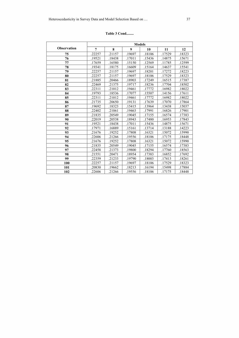
Table 3: Variable Weights for Observations
Observation Models
1 2 3 4 5 6
1 .34194 .29091 .27165 .25698 .25215 .23915
2 .34194 .29091 .27165 .25551 .25067 .23687
3 .33629 .28564 .25537 .24040 .22610 .21400
4 .34205 .29252 .27308 .25784 .25165 .23870
5 .34205 .27937 .25898 .24256 .23592 .22349
6 .34194 .29211 .27347 .25833 .25044 .23655
7 .33662 .28733 .26797 .25212 .24698 .23424
8 .34194 .29091 .27204 .25789 .25036 .23630
9 .33662 .28452 .26579 .25086 .24586 .22699
10 .33629 .28564 .26645 .24956 .24419 .23198
11 .34194 .29211 .26384 .23687 .23151 .21746
12 .34194 .29091 .27204 .25789 .23954 .22373
13 .34205 .29055 .27118 .25605 .24932 .23549
14 .34205 .29252 .27308 .25784 .25232 .24006
15 .34205 .29252 .27308 .25784 .25165 .23870
16 .34194 .29091 .26060 .24515 .23744 .22509
17 .34205 .29055 .27118 .25605 .24932 .23549
18 .34205 .29055 .27176 .25727 .24354 .23139
19 .32470 .27398 .25406 .23996 .23401 .22121
20 .34205 .29252 .27308 .25784 .24495 .23293
21 .34205 .29252 .27308 .25784 .25232 .24006
22 .34205 .29252 .26399 .24982 .24499 .23213
23 .34194 .29211 .27256 .25779 .24806 .23295
24 .34205 .29055 .25992 .24385 .23354 .22131
25 .34205 .27937 .26110 .24700 .24211 .22980
26 .34205 .29252 .27380 .25913 .25416 .24139
27 .34194 .29211 .27256 .25779 .25291 .24052
28 .32470 .27437 .25522 .24149 .23534 .19633
29 .34205 .29055 .27176 .25530 .24916 .23708
30 .34194 .29091 .27204 .25789 .25294 .24001
31 .34205 .29252 .27380 .25913 .24870 .23444
32 .34205 .29252 .27308 .25784 .25165 .23870
33 .34205 .29252 .27380 .25913 .25416 .24139
34 .34205 .29252 .27380 .24664 .23866 .20974
35 .34205 .29252 .26399 .24982 .24097 .22868
36 .34205 .29055 .27118 .25564 .25055 .23706
37 .33629 .28607 .26749 .25247 .24706 .23378

Heteroscedasticity in Survey Data and Model Selection Based on … 33
Table 3 Contd........
Observation Models
7 8 9 10 11 12
1 .20747 .19422 .17957 .16441 .15903 .16756
2 .22043 .20752 .19326 .17848 .17143 .17948
3 .19793 .18536 .17077 .15507 .14156 .17611
4 .22158 .20705 .19266 .17812 .17193 .18038
5 .20450 .19337 .17911 .15503 .14451 .15471
6 .22115 .20810 .19259 .17740 .17068 .17866
7 .21791 .20705 .19270 .17731 .17102 .17899
8 .22097 .20987 .19426 .17247 .15408 .16716
9 .20884 .19799 .18367 .15423 .14674 .15633
10 .21507 .20237 .17994 .16293 .15514 .16563
11 .20165 .18227 .16124 .14617 .13951 .15149
12 .20825 .19692 .18135 .16611 .12806 .14544
13 .22006 .20878 .19417 .17802 .17008 .18179
14 .22338 .20640 .18666 .16835 .16299 .17392
15 .22158 .21006 .19559 .16285 .15743 .16591
16 .20830 .19662 .18213 .16194 .15498 .17884
17 .22006 .20878 .15438 .13080 .12537 .13332
18 .21583 .20503 .18933 .17352 .16815 .17682
19 .20505 .19341 .17698 .16247 .15458 .16262
20 .21548 .20466 .18520 .16777 .16238 .17388
21 .22338 .21250 .19341 .17545 .16914 .17853
22 .21676 .19252 .17808 .16321 .15072 .15990
23 .21491 .20409 .18959 .17357 .16769 .17605
24 .20425 .19290 .16937 .15381 .14479 .16497
25 .21384 .20190 .18683 .16848 .15565 .16741
26 .22606 .21266 .19556 .18106 .17175 .18448
27 .22405 .21301 .19806 .18305 .17658 .18453
28 .17971 .16889 .15161 .13714 .13188 .14223
29 .22117 .14580 .13010 .11465 .10446 .11294
30 .22469 .21375 .19717 .18236 .17704 .18502
31 .21189 .20024 .18428 .16975 .16260 .17053
32 .22257 .21157 .19697 .18201 .17272 .18223
33 .22168 .20937 .19177 .17615 .16643 .18107
34 .17979 .16034 .14493 .12697 .12153 .12976
35 .21331 .19849 .17866 .16188 .11895 .12983
36 .22053 .20740 .19301 .17271 .16529 .17324
37 .21811 .20499 .18901 .17439 .16829 .17623

34 Journal of Reliability and Statistical Studies, Dec. 2013, Vol. 6(2)
Table 3 Cond........
Observation Models
1 2 3 4 5 6
38 .34205 .29252 .27308 .25770 .25123 .23752
39 .32470 .27398 .25406 .23996 .23410 .22192
40 .34205 .29055 .27176 .25530 .24916 .23440
41 .34205 .29055 .27176 .25727 .25139 .23767
42 .33629 .28564 .26645 .25214 .23541 .22025
43 .34205 .29055 .27176 .25530 .24217 .22964
44 .33629 .28607 .26636 .25197 .24697 .23440
45 .34194 .29211 .27256 .25779 .24806 .23295
46 .34194 .29211 .27256 .25659 .25175 .23882
47 .34205 .29252 .27380 .25771 .23215 .21992
48 .34194 .29091 .27204 .25485 .24996 .23759
49 .34205 .27937 .25898 .24435 .23917 .22510
50 .34205 .29252 .27308 .25770 .25235 .23965
51 .34205 .29055 .27176 .25530 .24916 .23708
52 .34205 .29252 .27380 .25771 .24670 .23467
53 .34205 .29055 .27176 .23899 .22599 .21276
54 .34205 .29252 .27308 .25784 .25232 .24006
55 .33662 .28452 .26501 .24929 .24288 .23028
56 .34205 .29055 .27118 .25605 .24932 .23549
57 .34205 .29252 .27308 .25770 .25235 .23965
58 .34205 .29252 .27308 .25784 .24495 .22934
59 .34194 .29091 .27204 .23738 .22763 .21412
60 .33662 .28733 .25829 .24008 .23465 .22040
61 .34205 .29252 .26399 .24672 .24187 .22952
62 .34194 .29211 .27256 .25659 .23617 .22031
63 .34194 .29091 .27204 .25485 .24690 .23170
64 .34194 .29091 .27204 .25789 .25294 .24001
65 .33629 .28564 .26665 .25275 .24486 .23247
66 .33662 .28452 .26579 .25086 .24586 .22699
67 .33662 .28452 .26501 .24929 .24288 .23028
68 .34194 .29091 .27204 .25485 .24996 .23626
69 .33629 .28607 .26749 .25247 .24706 .23444
70 .33629 .28607 .26749 .25247 .24706 .23378
71 .33662 .28452 .26579 .25086 .24003 .21095
72 .34205 .27937 .26110 .24700 .24211 .22817
73 .34205 .29252 .27380 .24664 .23866 .20974
74 .34205 .29252 .27308 .25784 .25165 .23870

Heteroscedasticity in Survey Data and Model Selection Based on … 35
Table 3 Cond........
Observation Models
7 8 9 10 11 12
38 .22011 .20821 .19294 .17690 .16988 .17784
39 .20517 .18985 .17386 .15902 .15121 .15927
40 .21885 .20466 .18903 .17249 .16515 .17387
41 .22236 .21144 .19507 .17464 .16911 .17832
42 .20384 .18900 .17017 .13879 .11768 .12582
43 .21323 .20203 .18643 .16828 .16262 .17351
44 .20614 .19355 .17506 .16001 .15435 .16659
45 .21724 .20142 .18059 .16493 .15240 .17354
46 .22311 .21012 .19461 .17772 .16982 .18022
47 .19830 .18616 .17068 .14487 .13810 .14691
48 .22139 .20991 .19297 .17796 .17193 .17987
49 .20930 .19596 .18162 .16708 .16041 .17332
50 .22141 .20983 .19465 .17928 .17308 .18107
51 .21955 .20734 .19086 .17048 .16408 .17327
52 .21591 .20489 .18867 .16991 .16131 .17077
53 .19692 .18323 .15415 .13964 .13438 .15037
54 .22359 .21233 .19790 .18344 .17810 .18677
55 .21445 .20354 .18591 .17043 .16429 .17692
56 .21649 .20448 .17765 .16196 .15522 .16354
57 .22141 .20703 .19205 .17654 .16915 .17988
58 .21094 .20014 .18585 .17120 .16594 .17489
59 .19643 .18339 .16893 .14914 .14383 .15340
60 .20509 .19320 .16173 .14333 .13759 .14798
61 .21020 .19600 .17676 .16155 .15625 .17848
62 .20375 .19082 .17445 .15898 .15317 .16267
63 .21282 .18480 .16756 .15256 .14558 .15388
64 .22019 .20538 .18943 .17480 .16953 .17843
65 .19836 .18489 .16844 .14756 .14220 .15238
66 .20884 .19799 .18367 .15423 .14674 .15633
67 .19961 .18583 .16929 .14635 .13976 .14914
68 .22050 .20873 .19065 .17429 .16892 .17686
69 .21835 .20549 .19045 .17155 .16574 .17383
70 .21565 .20110 .17049 .15585 .14333 .15191
71 .19521 .18438 .17011 .15436 .14875 .15671
72 .17659 .16580 .15150 .12569 .11785 .12599
73 .19341 .18175 .16609 .15164 .14637 .15541
74 .22257 .21157 .19697 .18201 .17272 .18223

36 Journal of Reliability and Statistical Studies, Dec. 2013, Vol. 6(2)
Table 3 Cond........
Observation Models
1 2 3 4 5 6
75 .34205 .29252 .27308 .25784 .25165 .23870
76 .33662 .28452 .26579 .25086 .24003 .21095
77 .34205 .27937 .26110 .24700 .24211 .22817
78 .34205 .29252 .27380 .24664 .23866 .20974
79 .34205 .29252 .27308 .25784 .25165 .23870
80 .34205 .29252 .27308 .25784 .25165 .23870
81 .34205 .29055 .27176 .25530 .24916 .23440
82 .34194 .29091 .27204 .25789 .25294 .24001
83 .34194 .29211 .27256 .25659 .25175 .23882
84 .33629 .28564 .25537 .24040 .22610 .21400
85 .34194 .29211 .27256 .25659 .25175 .23882
86 .34194 .29091 .27204 .25789 .25036 .23284
87 .34205 .29055 .27176 .23899 .22599 .21276
88 .34205 .29252 .27380 .25913 .25167 .23935
89 .33629 .28607 .26749 .25247 .24706 .23444
90 .34194 .29091 .27204 .25789 .25294 .24001
91 .33662 .28452 .26579 .25086 .24003 .21095
92 .32470 .27437 .25522 .24149 .23534 .19633
93 .34205 .29252 .26399 .24982 .24499 .23213
94 .34205 .29252 .27380 .25913 .25416 .24139
95 .34205 .29252 .26399 .24982 .24499 .23213
96 .33629 .28607 .26749 .25247 .24706 .23444
97 .34194 .29091 .27204 .25789 .25294 .24005
98 .33662 .28452 .26579 .25086 .24346 .23092
99 .34205 .29252 .27308 .25784 .25232 .24006
100 .34205 .29252 .27308 .25784 .25165 .23870
101 .34194 .29091 .26060 .24515 .23744 .22509
102 .34205 .29252 .27380 .25913 .25416 .24139
Heteroscedasticity in Survey Data and Model Selection Based on … 37
Table 3 Cond........
Observation Models
7 8 9 10 11 12
75 .22257 .21157 .19697 .18106 .17529 .18323
76 .19521 .18438 .17011 .15436 .14875 .15671
77 .17659 .16580 .15150 .12569 .11785 .12599
78 .19341 .18175 .16609 .15164 .14637 .15541
79 .22257 .21157 .19697 .18201 .17272 .18223
80 .22257 .21157 .19697 .18106 .17529 .18323
81 .21885 .20466 .18903 .17249 .16515 .17387
82 .22469 .21375 .19717 .18236 .17704 .18502
83 .22311 .21012 .19461 .17772 .16982 .18022
84 .19793 .18536 .17077 .15507 .14156 .17611
85 .22311 .21012 .19461 .17772 .16982 .18022
86 .21735 .20650 .19131 .17639 .17070 .17864
87 .19692 .18323 .15415 .13964 .13438 .15037
88 .22402 .21061 .19463 .17991 .16826 .17901
89 .21835 .20549 .19045 .17155 .16574 .17383
90 .22019 .20538 .18943 .17480 .16953 .17843
91 .19521 .18438 .17011 .15436 .14875 .15671
92 .17971 .16889 .15161 .13714 .13188 .14223
93 .21676 .19252 .17808 .16321 .15072 .15990
94 .22606 .21266 .19556 .18106 .17175 .18448
95 .21676 .19252 .17808 .16321 .15072 .15990
96 .21835 .20549 .19045 .17155 .16574 .17383
97 .22458 .21373 .19800 .18294 .17760 .18563
98 .21551 .20471 .18954 .17383 .16852 .17692
99 .22359 .21233 .19790 .18003 .17413 .18261
100 .22257 .21157 .19697 .18106 .17529 .18323
101 .20830 .19662 .18213 .16194 .15498 .17884
102 .22606 .21266 .19556 .18106 .17175 .18448

38 Journal of Reliability and Statistical Studies, Dec. 2013, Vol. 6(2)
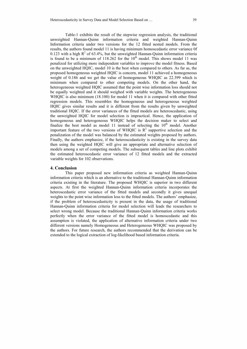
Lineplot shows the information loss of Models based on no.of parameters and
Heteoscedastic error variance, Weights for observations
Heteroscedasticity in Survey Data and Model Selection Based on … 39
Table-1 exhibits the result of the stepwise regression analysis, the traditional
unweighted Hannan-Quinn information criteria and weighted Hannan-Quinn
Information criteria under two versions for the 12 fitted nested models. From the
results, the authors found model 11 is having minimum homoscedastic error variance 0f
0.123 with a high R2 of 63.4%, but the unweighted Hannan-Quinn information criteria
is found to be a minimum of 118.262 for the 10th
model. This shows model 11 was
penalized for utilizing more independent variables to improve the model fitness. Based
on the unweighted HQIC, model 10 is the best when compared to others. As far as, the
proposed homogeneous weighted HQIC is concern, model 11 achieved a homogeneous
weight of 0.186 and we get the value of homogeneous WHQIC as 22.399 which is
minimum when compared to other competing models. On the other hand, the
heterogeneous weighted HQIC assumed that the point wise information loss should not
be equally weighted and it should weighed with variable weights. The heterogeneous
WHQIC is also minimum (18.100) for model 11 when it is compared with other fitted
regression models. This resembles the homogeneous and heterogeneous weighted
HQIC gives similar results and it is different from the results given by unweighted
traditional HQIC. If the error variances of the fitted models are heteroscedastic, using
the unweighted HQIC for model selection is impractical. Hence, the application of
homogeneous and heterogeneous WHQIC helps the decision maker to select and
finalize the best model as model 11 instead of selecting the 10th
model. Another
important feature of the two versions of WHQIC is R2 supportive selection and the
penalization of the model was balanced by the estimated weights proposed by authors.
Finally, the authors emphasize, if the heteroscedasticity is existing in the survey data
then using the weighted HQIC will give an appropriate and alternative selection of
models among a set of competing models. The subsequent tables and line plots exhibit
the estimated heteroscedastic error variance of 12 fitted models and the extracted
variable weights for 102 observations.
4. Conclusion This paper proposed new information criteria as weighted Hannan-Quinn
information criteria which is an alternative to the traditional Hannan-Quinn information
criteria existing in the literature. The proposed WHQIC is superior in two different
aspects. At first the weighted Hannan-Quinn information criteria incorporates the
heteroscedastic error variance of the fitted models and secondly it gives unequal
weights to the point wise information loss to the fitted models. The authors’ emphasize,
if the problem of heteroscedasticity is present in the data, the usage of traditional
Hannan-Quinn information criteria for model selection will leads the researchers to
select wrong model. Because the traditional Hannan-Quinn information criteria works
perfectly when the error variance of the fitted model is homoscedastic and this
assumption is violated, the application of alternative information criteria under two
different versions namely Homogeneous and Heterogeneous WHQIC was proposed by
the authors. For future research, the authors recommended that the derivation can be
extended to the logical extraction of log-likelihood based information criteria.

40 Journal of Reliability and Statistical Studies, Dec. 2013, Vol. 6(2)
References
1. Arlot, S., (2012). Choosing a penalty for model selection in heteroscedastic
regression, Arxiv preprint arXiv:0812.3141.
2. Andrew Barron, Lucien Birg´e, and Pascal Massart (1999). Risk bounds for
model selection via penalization, Probab. Theory Related Fields, 113(3), p.
301–413.
3. Boris T. Polyak and Tsybakov, A.B. (1990). Asymptotic optimality of the Cp-
test in the projection estimation of a regression, Teor. Veroyatnost. i
Primenen., 35(2), p.305–317.
4. Corderio, G.M, (2008). Corrected maximum likelihood estimators in linear
heteroscdastic regression models, Brazilian Review of Econometrics, 28, p. 1-
18.
5. Colin L. Mallows (1973). Some comments on Cp. Technometrics, 15, p. 661–
675.
6. Fisher, G.R., (1957). Maximum likelihood estimators with heteroscedastic
errors, Revue de l’Institut International de statistique, p. 52-55.
7. Greene and William H. Greene (2011). Econometric Analysis, Pearson
Education Ltd.
8. Hirotugu Akaike (1970). Statistical predictor identification. Ann. Inst. Statist.
Math., 22, p. 203–217.
9. Hirotugu Akaike (1973). Information theory and an extension of the maximum
likelihood principle. In Second International Symposium on Information
Theory (Tsahkadsor, 1971), p. 267–281, Akad´emiai Kiad´o, Budapest.
10. Ker-Chau Li (1987). Asymptotic optimality for Cp, CL, cross-validation and
generalized crossvalidation: discrete index set, Ann. Statist., 15(3), p. 958–
975.
11. Lucien Birg´e and Pascal Massart (2007). Minimal penalties for Gaussian
model selection, Probab. Theory Related Fields, 138(1-2), p. 33–73.
12. Muralidharan, K. and Kale, B. K. (2008). Inliers detection using schwartz
information criterion, Journal of Reliability and Statistical Studies, 1(1), p. 1-
5.
13. Myers, R. H. and Montgomery, D,C. (1997). A Tutorial on Generalized Linear
Models, Journal of Quality Technology, 29, p. 274-291.
14. Ritei Shibata (1981). An optimal selection of regression variables, Biometrika,
68(1), p.45–54.
15. Sylvain Arlot (2009). Model selection by resampling penalization, Electron. J.
Stat., 3:557–624.
16. Xavier Gendre (2008). Simultaneous estimation of the mean and the variance
in heteroscedastic Gaussian regression, Electron. J. Stat., 2, p. 1345–1372.
17. Yannick Baraud (2000). Model selection for regression on a fixed design,
Probab. Theory Related Fields, 117(4), p. 467–493.
18. Yannick Baraud (2002). Model selection for regression on a random design,
ESAIM Probab. Statist., 6, p. 127–146 (electronic).