A Powerful test for conditional heteroscedasticity for financial time series with highly persistent...

Statistica Sinica 15(2005), 505-525

A POWERFUL TEST FOR CONDITIONAL

HETEROSCEDASTICITY FOR FINANCIAL TIME SERIES

WITH HIGHLY PERSISTENT VOLATILITIES

Julio Rodrıguez and Esther Ruiz

Universidad Politecnica de Madrid and Universidad Carlos III de Madrid

Abstract: Traditional tests for conditional heteroscedasticity are based on testing

for significant autocorrelations of squared or absolute observations. In the context

of high frequency time series of financial returns, these autocorrelations are often

positive and very persistent, although their magnitude is usually very small. More-

over, the sample autocorrelations are severely biased towards zero, especially if the

volatility is highly persistent. Consequently, the power of the traditional tests is

often very low. In this paper, we propose a new test that takes into account not

only the magnitude of the sample autocorrelations but also possible patterns among

them. This additional information makes the test more powerful in situations of

empirical interest. The asymptotic distribution of the new statistic is derived and

its finite sample properties are analyzed by means of Monte Carlo experiments. The

performance of the new test is compared with various alternative tests. Finally, we

illustrate the results analyzing several time series of financial returns.

Key words and phrases: Autocorrelations of non-linear transformations, GARCH,

long-memory, McLeod-Li statistic, stochastic volatility.

1. Introduction

It is well known that high frequency time series of returns are characterizedby evolving conditional variances. As a consequence, some non-linear transfor-mations of returns, such as squares or absolute values, are autocorrelated. Thecorresponding autocorrelations are often small, positive and decay very slowlytowards zero. This last characteristic has usually been related to long-memoryin volatility; see, for example, Ding, Granger and Engle (1993). Two of the mostpopular models to represent the dynamic evolution of volatilities are the Gener-alized Autoregressive Conditional Heteroscedasticity (GARCH) model of Engle(1982) and Bollerslev (1986) and the Autoregressive Stochastic Volatility (ARSV)model proposed by Taylor (1984). Both models generate series with autocorre-lated squares. However, Carnero, Pena and Ruiz (2004a) show that, unless thekurtosis is heavily restricted, GARCH models are not able to represent auto-correlations as small as those often observed in practice. Furthermore, little isknown about the autocorrelations of squared or absolute returns generated by the

504 JULIO RODRIGUEZ AND ESTHER RUIZ

most popular long-memory GARCH model, the Fractionally Integrated GARCH

(FIGARCH) model proposed by Baillie, Bollerslev and Mikkelsen (1996); see

Karanasos, Psaradakis and Sola (2004) and Palma and Zevallos (2004) for the

autocorrelations of squares of long memory GARCH models closely related to

FIGARCH. Moreover, Davidson (2004) shows that the dynamic properties of

the FIGARCH model are somehow unexpected in the sense that the persistence

of the volatility is larger the closer the long memory parameter is to zero. On

the other hand, ARSV models are more flexible in representing the empirical

characteristics often observed in high frequency returns and the statistical prop-

erties of the model are well defined. In particular, Harvey (1998) derives the

autocorrelations of powers of absolute observations of Long Memory Stochastic

Volatility (LMSV) models. Consequently, in this paper, we focus on testing for

conditional homoscedasticity in the context of Stochastic Volatility (SV) models.

For the reasons previously given, the identification of conditional heter-

oscedasticity is often based on testing whether squared or absolute returns are

autocorrelated; see, for example, Andersen and Bollerslev (1997) and Bollerslev

and Mikkelsen (1999) among many others. Testing for lack of correlation of a

particular transformation of returns, f(yt), can be carried out using the port-

manteau statistic suggested by Ljung and Box (1978),

Q(M) = TM∑

k=1

r2(k), (1.1)

where r(k) =√

(T + 2)/(T − k)r(k) is the standardized sample autocorrela-

tion of order k, r(k) =∑T

t=k+1(f(yt) − f)(f(yt−k) − f)/∑T

t=1(f(yt) − f)2, f =∑Tt=1 f(yt)/T , and T is the sample size. In this paper, we consider two popular

transformations, namely f(yt) = y2t and f(yt) = |yt|.

The Q(M) statistic applied to squared observations was proposed by McLeod

and Li (1983) who show that, if the eighth order moment of yt exists, its asymp-

totic distribution can be approximated by a χ2(M) distribution. From now on, the

statistic in (1) is named the McLeod-Li statistic even if it is applied to absolute

returns. Notice that the χ2(M) asymptotic distribution of the Ljung-Box statistic

requires that the series to be tested for uncorrelation is an independent sequence

with finite fourth order moment; see Hannan (1970). Therefore, when the Q(M)

statistic is implemented with absolute values, only the fourth order moment of

returns should be finite for the asymptotic distribution to hold.

Alternatively, Pena and Rodriguez (2002) proposed a portmanteau test based

on the Mth root of the determinant of the autocorrelation matrix of order M ,

DM = T[1 − |RM |1/M

], (1.2)

A POWERFUL TEST FOR CONDITIONAL HETEROSCEDASTICITY 505

where

RM =

1 r(1) · · · r(M)r(1) 1 · · · r(M − 1)

......

......

r(M) r(M − 1) · · · 1

.

Pena and Rodriguez (2005a) have proposed a modified version of the DM statistic

based on the logarithm of the determinant. This new statistic has better size

properties for large M and better power properties. If the eighth order moment

of yt exists, the asymptotic distribution of the DM statistic applied to squared

observations can be approximated by a Gamma distribution, G(θ, τ), with θ =

3M(M + 1)/4(2M + 1) and τ = 3M/2(2M + 1). The same result holds for

absolute values if the fourth order moment of returns is finite.

Although Pena and Rodriguez (2002) show that in general, for squared re-

turns, the DM test is more powerful than the McLeod-Li test, both tests have

rather low power, especially when the volatility is very persistent; see, Perez and

Ruiz (2003) for exhaustive Monte Carlo experiments in the context of LMSV

models. The low power could be attributed to substantial finite sample negative

biases of the sample autocorrelations and to the small magnitude of the popula-

tion autocorrelations. Therefore, these tests may fail to reject homoscedasticity

when the returns are conditionally heteroscedastic.

However, notice that the sample autocorrelations of independent series with

finite fourth order moment are asymptotically, not only identically distributed

normal variables with zero mean and variance 1/T , but also mutually indepen-

dent; see Hannan (1970). Therefore, the estimated autocorrelations are not ex-

pected to have any distinct pattern in large samples. However, the McLeod-Li

and Pena-Rodriguez tests only focus on the first implication of the null hypothe-

sis, namely that the sample autocorrelations should have zero mean. These tests

ignore the information on the patterns of successive estimated autocorrelations

and, consequently, cannot distinguish between the correlogram of an uncorrelated

variable whose autocorrelation coefficients are small and randomly distributed

around zero, and the correlogram of a variable that has relatively small autocor-

relations with a distinct pattern for very long lags. In this paper, we propose

using a new statistic that considers the information about possible patterns in

successive correlations to test for uncorrelatedness in non-linear transformations

of returns . This test is based on ideas developed by Koch and Yang (1986) in

the context of testing for zero cross-correlations between series of multivariate

dynamic systems.

Finally, given that we are analyzing the performance of tests for conditional

homoscedasticity in the context of SV models, we also consider the test proposed


by Harvey and Streibel (1998) who focus on the ARSV(1) model given by

yt = σ∗εtσt, t = 1, . . . , T,(1.3)

log(σ2t ) = φ log(σ2

t−1) + ηt,

where σ∗ is a scale parameter, σt is the volatility, and εt and ηt are mutually

independent Gaussian white noise processes with zero mean and variances one

and σ2η, respectively. The model is stationary if |φ| < 1. The same condition

guarantees the existence of the fourth order moment; see Ghysels, Harvey and

Renault (1996) for a detailed description of the statistical properties of SV mod-

els. The variance of the log-volatility process is given by σ2h = σ2

η/(1 − φ2), and

it is assumed to be finite and fixed. Therefore, the variance of ηt can be written

as a function of the persistence parameter as σ2η = (1 − φ2)σ2

h. Observe that if,as is often observed in real time series of high frequency returns, the persistence

parameter φ is close to one, then σ2η should be close to zero for a given value of

the variance of log(σ2t ). In this case, the volatility evolves very smoothly through

time. In the limit, if φ = 1 then σ2η = 0 and yt is conditionally homoscedastic.

Harvey and Streibel (1998) propose testing σ2η = 0 using

NM = −T−1T−1∑

k=1

r(k)k. (1.4)

They show that if the second order moment of f(yt) is finite, the NM statistic

has asymptotically the Cramer-von Mises distribution, for which the 5% critical

value is 0.461. Furthermore, the corresponding test is the Locally Best Invariant

(LBI) test for the presence of a random walk; see Ferguson (1967) for the defini-

tion of the Locally Best test. They implement the test on squared and absolute

observations, and show that the finite sample power is higher when the latter

transformation is used.

The paper is organized as follows. Section 2 describes the new statistic andderives its asymptotic distribution under the null hypothesis. In Section 3, we

carry out Monte Carlo experiments to assess the finite sample size and power

of the new statistic in short memory ARSV and LMSV models. These finite

sample properties are compared with the properties of the McLeod-Li, Pena-

Rodriguez and Harvey-Streibel tests. In Section 4, the test is used to test for

uncorrelatedness in squared and absolute daily returns of several financial prices.

2. A New Test for Conditional Homoscedasticity

As mentioned earlier, conditionally heteroscedastic processes generate time

series with autocorrelated squares and absolute observations. Consequently, we

propose testing for conditional homoscedasticity using the information contained


in the sample autocorrelations of non-linear transformations, f of the underly-ing process yt. The new test for zero correlations of f(yt) takes into account

that, under the null hypothesis, if the fourth order moment of f(yt) exists, thesample autocorrelations of f(yt) are asymptotically independent and identicallydistributed normal variables with zero mean and variance 1/T . Therefore, this

statistic not only tests whether the sample autocorrelations are significantly dif-ferent from zero but also incorporates information about possible patterns amongsuccessive autocorrelation coefficients, r(k). We propose the statistic

Q∗

i (M) = TM−i∑

k=1

[ i∑

l=0

r(k + l)]2

, i = 0, . . . ,M − 1, (2.1)

where r(k + l) is the standardized sample autocorrelation of order k + l. Noticethat for each value of the number of autocorrelations considered, M , we have acollection of statistics, choosing different values of i. Each of these statistics has

different information on the possible pattern of the sample autocorrelations. Forexample, when i = 0, the McLeod-Li statistic in (1) is obtained as a particular

case. In this case, the statistic is obtained adding up the squared estimatedautocorrelations. If all of these autocorrelations are small, the statistic will besmall and the null hypothesis is not rejected. However, when i = 1, the statistic

incorporates information about the correlation between sample autocorrelationsone lag apart. In this case, if they are strongly correlated, the null hypothesiscan be rejected even if the coefficients r(j) are very small. When i = 2, the

correlations between coefficients two lags apart are also considered, and so on.The statistic Q∗

i (M) is a quadratic form in T 1/2r(M), r(M) =(r(1), . . . , r(M)),

given by

Q∗

i (M) = T r′

(M)Air(M),

where Ai = C′

iCi is a symmetric matrix of dimension M. In general C′

i is amatrix of dimension M × (M − i), where the jth column has j−1 zeroes followedby i + 1 ones, followed by zeroes. Given that, under the null hypothesis, the

asymptotic distribution of T 1/2r(M) is N(0, IM ), Q∗

i (M) behaves asymptoticallyas

Q(W ) ∼M∑

i=1

λiχ2(1),i,

where χ2(1),i are independent chi-squared variables with one degree of freedom,

and the λj are the eigenvalues of Aj; see Box (1954). Therefore, the asymp-totic distribution of Q∗

i (M) depends on the eigenvalues of Ai, and consequently

on M and i. Although the percentiles of the asymptotic distribution can bedirectly obtained, it is easier to compute them using one of the following two

approximations. The first is from Satterthwaite (1941, 1946) and Box (1954).


In particular, the distribution of Q∗

i (M) can be approximated by a gammadistribution, G(θ, τ), with parameters θ = a2/2b and τ = a/2b, where a =(i + 1)(M − i) and b = (M − i)(i + 1)2 + 2

∑i+1j=1(M − i − j)(i + 1 − j)2. Notice

that a is the trace of the matrix Ai, tr(Ai) =∑M

j=1 λj , and b the trace of AiAi,

tr(AiAi) =∑M

j=1 λ2j . For example, if i = 0, then a = M , b = M , and therefore

the usual χ2(M) asymptotic distribution is obtained. On the other hand, if for

instance i = 1, then the parameters of the Gamma distribution are given byθ = (M−1)2/(3M−4) and τ = (M−1)/(3M−4). For reasons that will be madeclearer later, another interesting case is i = [M/3]−1. In this case, the corre-sponding parameters are θ = (54M+72M 2+24M3)/2(45M+12M 2+7M3+54))and τ = (108M+162)/(45M + 12M 2+7M3+54). Finally, consider the casei=M−1, with θ =−6M/2(M 3−4M2−M−2) and τ =−6/(M 3−4M2−M−2).Here the asymptotic distribution of the statistic Q∗

M−1(M)/M can be approxi-mated by χ2

(1).

The asymptotic distribution of Q∗

i (M) can alternatively be approximatedusing the generalization of the Wilson-Hilferty cube root transformation for χ2

random variables. This generalization has been proposed by Chen and Deo (2004)to improve the normality of test statistics in finite samples. In particular, theyprovide an expression for the appropriate value of a power transformation, β,that makes the approximate skewness zero. The asymptotic distribution of thetransformed statistic Q∗

i (M)β is then given by

Q∗

i (M)β − {aβ + β(β − 1)aβ−2b}βaβ−1

√2b

∼ N(0, 1),

where β = 1− 2ac/3b2, c = tr(AiAiAi), and the parameters a and b are definedas in the previous approximation. Finally, notice that once M and i have beenchosen, all the parameters needed to obtain the normal transformed statistic aregiven.

3. Size and Power in Finite Samples

In this section, we analyze the finite sample performance of the Q∗

i (M) statis-tic by means of Monte Carlo experiments. The main objectives are to investigatewhether the asymptotic distribution is an adequate approximation to the finitesample distribution under the null hypothesis, and to compare the size and powerof the new statistic with the McLeod-Li, Pena-Rodriguez and Harvey-Streibelstatistics. Furthermore, we give some guidelines as to which values of M and iwork well from an empirical point of view.

3.1 Size

To analyze the size of the test in finite samples, we have generated series ofwhite noise processes with two different distributions, Normal and Student-t with


ν = 5 degrees of freedom. The Student-t distributions have been chosen because

it has been often observed in empirical applications that the marginal distribution

of financial returns is leptokurtic, and we want to analyze the performance of the

tests in the presence of leptokurtic, homoscedastic time series. Moreover, the

degrees of freedom are selected in such a way that the eighth moment of returns

exists when ν = 9, and does not exit when ν = 5. All results are based on 20,000

replicates.

Table 1. Empirical sizes of the Q(M), DM , NM and Q∗i (M) tests, i =

1, [M/3]−1 and M−1 for squared and absolute observations of homoscedastic

Gaussian noise series of size T = 50, 100, 500 and 2, 000.

y2t |yt|

M\T 50 100 500 2,000 50 100 500 2,000

12 DM 0.029 0.037 0.048 0.050 0.042 0.043 0.051 0.050

Q(M) 0.058 0.057 0.048 0.050 0.068 0.055 0.053 0.048

Q∗1(M) 0.055 0.055 0.048 0.048 0.065 0.057 0.052 0.053

Q∗3(M) 0.049 0.050 0.045 0.049 0.054 0.052 0.049 0.051

Q∗11(M) 0.013 0.025 0.040 0.046 0.014 0.026 0.044 0.047

24 DM 0.021 0.027 0.045 0.048 0.029 0.032 0.048 0.049Q(M) 0.074 0.069 0.054 0.051 0.089 0.070 0.058 0.050

Q∗1(M) 0.077 0.073 0.056 0.052 0.090 0.075 0.059 0.054

Q∗7(M) 0.053 0.053 0.046 0.049 0.055 0.053 0.051 0.049

Q∗23(M) 0.002 0.013 0.034 0.046 0.002 0.015 0.039 0.045

36 DM 0.009 0.019 0.041 0.048 0.013 0.022 0.050 0.049Q(M) 0.071 0.081 0.059 0.051 0.087 0.083 0.062 0.052

Q∗1(M) 0.083 0.087 0.059 0.056 0.101 0.092 0.064 0.054

Q∗11(M) 0.054 0.052 0.049 0.050 0.057 0.056 0.052 0.051

Q∗35(M) 0.001 0.007 0.028 0.043 0.001 0.006 0.033 0.045

NM 0.047 0.049 0.050 0.047 0.050 0.050 0.053 0.051

Table 1 reports the empirical sizes of the DM , Q(M), NM and Q∗

i (M) tests

when the series are generated by homoscedastic Gaussian white noise processes.

We consider M = 12, 24 and 36 and i = 1, [M/3]−1 and M−1. The nominal size

is 5% and the sample sizes are T = 50, 100, 500 and 2, 000. The critical values

have been obtained using the Gamma and Normal approximations described in

Section 2, with similar results. Therefore, Table 2 only reports the empirical sizes

obtained using the Gamma distribution. All the statistics are implemented for

both squared and absolute observations. The results reported in Table 1 show

that, with the exception of Q∗

M−1(M), the empirical size of all tests considered

is very close to the nominal one for moderate sample size. However, when the

sample size is small, T = 50, 100, only the Q∗

[M/3]−1(M) and NM tests have sizes

reasonably close to the nominal.


Table 2. Empirical sizes of Q(M), DM , NM and Q∗i (M) tests, i = 1, [M/3]−1

and M−1 for squared and absolute observations of homoscedastic Student-5

noise series of size T = 50, 100, 500 and 2, 000.

y2t |yt|

M\T 50 100 500 2,000 50 100 500 2,000

12 DM 0.024 0.036 0.061 0.069 0.032 0.036 0.047 0.051

Q(M) 0.034 0.040 0.065 0.074 0.044 0.047 0.051 0.054Q∗

1(M) 0.030 0.035 0.052 0.061 0.040 0.045 0.049 0.053

Q∗3(M) 0.025 0.029 0.039 0.048 0.032 0.038 0.047 0.051

Q∗11(M) 0.008 0.016 0.028 0.037 0.009 0.021 0.041 0.048

24 DM 0.014 0.026 0.064 0.078 0.024 0.027 0.044 0.049

Q(M) 0.033 0.040 0.064 0.086 0.050 0.055 0.054 0.055

Q∗1(M) 0.039 0.041 0.055 0.073 0.056 0.054 0.054 0.054

Q∗7(M) 0.027 0.031 0.032 0.045 0.037 0.040 0.048 0.049

Q∗23(M) 0.001 0.009 0.023 0.036 0.001 0.010 0.036 0.046

36 DM 0.006 0.016 0.062 0.082 0.010 0.019 0.039 0.048

Q(M) 0.027 0.043 0.063 0.089 0.041 0.059 0.056 0.053

Q∗1(M) 0.039 0.045 0.053 0.079 0.055 0.064 0.059 0.056

Q∗11(M) 0.032 0.035 0.030 0.044 0.040 0.042 0.050 0.048

Q∗35(M) 0.000 0.004 0.020 0.034 0.001 0.005 0.031 0.043

NM 0.039 0.041 0.044 0.046 0.048 0.049 0.048 0.049

Figure 1 plots the differences between the empirical and nominal sizes of the

Q∗

i (M) test as a function of i for M = 12, 24 and 36, and T = 500, 1, 000, 2, 000,

and 4, 000. This figure shows that whatever the sample size is, the empirical size

of the test is closer to the nominal size of 5% when i is chosen to be approximately

equal to [M/3] − 1. Similar results have been obtained for other nominal sizes.

Table 2 reports the same quantities as in Table 1 when the series are gen-

erated by homoscedastic Student-5 white noises. In this case, it is possible to

observe that all the tests considered can suffer from important size distortions

when they are applied to squared observations. The empirical size is larger than

the nominal for the DM , Q(M) and Q∗

i (M) tests with small values of i. Con-

sequently, the tests would reject the hypothesis of homoscedasticity more often

than expected. Furthermore, the size distortions are not reduced when the sam-

ple size increases. For example, the sizes of D24, Q(24) and Q∗

1(24) are 6.4%,

6.4% and 5.5%, respectively, when T = 500, and 7.8%, 8.6% and 7.3% when

T = 2, 000. Therefore it is evident that, as expected when the eighth moment

is not defined, the asymptotic distribution is a bad approximation to the finite

sample distribution of the statistics considered. The size distortions of Q∗

i (M)

are smaller than those for the Q(M) and DM tests, but they are still big enough

to matter. Figure 2, which plots the differences between empirical and nominal

sizes of Q∗

i (M), i = 0, . . . ,M − 1 and M = 12, 24 and 36, illustrates these size


distortions. On the other hand, notice that the asymptotic distribution of the

NM test only requires the second moment of yt to be finite and consequently, as

reflected in Table 2, its size is close to the nominal. Finally, Table 2 shows that

when the tests are applied to absolute observations, the nominal and empirical

sizes of all the tests considered are very close; see also Figure 2, which shows

that the size of Q∗

i (M) is rather close to the nominal for all M and i, even for

moderate sample sizes.

PSfrag replacements

-1

-2

-0.05

-0.1

0.05

2

1

22 44

55

66

7

88

10

10

10

10

10

10 1212

1515

20

20

20

20

25

3030

40

50

200

400

600

800

0

0.1

0.15

0.2

0.25

0.3

0.35

0.4

0.45

0.5

0.6

0.7

0.8

0.9

d

1

0.82

0.84

0.86

0.88

0.92

0.94

0.96

0.98

0.040

0.040

0.040

0.040

0.040

0.040

0.0420.042

0.0440.044

0.0460.046

0.0480.048

0.050

0.050

0.050

0.050

0.050

0.050

0.0520.052

0.035

0.035

0.035

0.035

0.045

0.045

0.045

0.045

0.055

0.055

0.055

0.055

0.0300.030

0.0600.060

Series Y 2t

Series Y 2t

Series Y 2t with Gaussian noise, m=12with Gaussian noise, m=12

with Gaussian noise, m=24with Gaussian noise, m=24

with Gaussian noise, m=36with Gaussian noise, m=36 Series |Yt|

Series |Yt|

Series |Yt|

(a) Canadian dollar

(b) EURO

(c) Swiss francLMSV(φ = 0.9, d, σ2

η = 0.01)

LMSV(φ = 0, d, σ2η = 0.1)

Figure 1. Differences between empirical and nominal rejection probabilities,

α = 0.05, of the Q∗i (M) test, i = 0, . . . , M−1, for non-linear transformations

of Gaussian noises with T=500 (· · ·), T = 1, 000 (−·), T = 2, 000 (−−) and

T = 4, 000 (—).


PSfrag replacements

-1

-2

-0.05

-0.1

0.05

2

1

22 44

5

5

5

5

66

7

88

10

10

10

10

10

10 1212

1515

20

20

20

20

25

3030

40

50

200

400

600

800

0

0.1

0.15

0.2

0.25

0.3

0.35

0.4

0.45

0.5

0.6

0.7

0.8

0.9

d

1

0.82

0.84

0.86

0.88

0.92

0.94

0.96

0.98

0.040

0.042

0.044

0.046

0.048

0.050

0.052

0.035

0.045

0.055

0.030

0.060

Series Y 2t

Series Y 2t

Series Y 2t

with Gaussian noise, m=12



Series |Yt|

Series |Yt|

Series |Yt|

(a) Canadian dollar

(b) EURO


η = 0.01)

LMSV(φ = 0, d, σ2η = 0.1)

0.02

0.03

0.03

0.03

0.03

0.03

0.03

0.04

0.04

0.04

0.04

0.04

0.04

0.05

0.05

0.05

0.05

0.05

0.05

0.06

0.06

0.06

0.06

0.06

0.06

0.07

0.07

0.07

0.07

0.07

0.07

0.08

0.08

0.08

0.08

0.090.09

with Student-t5

with Student-t5

with Student-t5

with Student-t5

with Student-t5

with Student-t5 noise, m=12noise, m=12

noise, m=24noise, m=24

noise, m=36noise, m=36

Figure 2. Differences between empirical and nominal rejection probabilities,α = 0.05, of the Q∗

i (M) test, i = 0, . . . , M−1, for non-linear transformationsof Student-t5 noises with T = 500 (· · ·), T = 1, 000 (−·), T = 2, 000 (−−)and T = 4, 000 (—).

Focusing now on the results for absolute observations, Figures 1 and 2, the

empirical sizes of Q∗

i (M) decrease with i. For M = 12, 24 and 36, the smallest

differences are obtained when i is approximately 3, 5 and 11 respectively. There-

fore, it seems that the size is close to the nominal if i = [M/3] − 1. In any case,

it is important to point out that for all values of M and i considered, the size of

Q∗

i (M) is remarkably close to the nominal, especially for large sample sizes.

Summarizing, the Monte Carlo experiments reported in this section show


that, if i = [M/3] − 1 and the fourth order moment of yt exists, the asymptotic

distribution provides an adequate approximation to the sample distribution of

Q∗

i (M) when it is applied to absolute returns. If this is implemented with squared

observations, the eighth moment should be finite. Consequently, we recommend

testing for conditional heteroscedasticity using absolute returns; see also Harvey

and Streibel (1998) and Perez and Ruiz (2003). From now on, in this paper, all

results are based on implementing the various statistics considered with absolute

observations.

3.2. Power for short memory models

To analyze the power of Q∗

i (M) in finite samples, we have generated artificial

series by the ARSV(1) in (1.3) for squared C.V. = exp(σ2h) − 1 = 0.22, 0.82

and 1.72. These values have been chosen to resemble the parameter values often

estimated when the ARSV model is fitted to time series of financial returns; see

Jacquier, Polson and Rossi (1994). The sample sizes considered are T = 100,

512 and 1, 024. The scale parameter σ∗ has been fixed to one without loss of

generality.

Figure 3 plots the percentage of rejections of the Q(M), DM , NM and

Q∗

i (M) tests as a function of the persistence parameter, φ, for M = 24 and

T = 100 and 512. Remember that when φ = 1, σ2η = 0 and, consequently, given

that the series are homoscedastic, the percentage of rejections is 5%. First of

all, this figure shows that the power of the NM test is highest when φ is close

to the boundary and, consequently, the series is close to the null hypothesis of

homoscedasticity, and when the sample size is very small. When the persistence of

volatility decreases or the sample size is moderately large, the NM has important

losses of power relative to its competitors. Notice that for the sample sizes usually

encountered in the empirical analysis of financial time series, the powers of the

Q(M), DM and Q∗

i (M) tests are larger than the power of NM . On the other

hand, comparing the powers of Q(M), DM and Q∗

i (M), we can observe that if

the sample size is T = 100, the power of Q∗

i (M) is the largest for all the values

of the parameters considered in Figure 3, i.e., φ ≥ 0.8. Finally, if T = 512, the

power of Q∗

i (M) is larger when C.V. = 0.22, and very similar for the other two

C.V. considered. The powers of the three tests are similar and close to one for

large sample sizes.

To illustrate how the proposed test has higher power than its competitors,

even in the more persistent cases, when the McLeod-Li and Pena-Rodriguez tests

are well known to have difficulties in identifying the presence of conditional het-

eroscedasticity, Table 3 reports the powers of these tests using absolute observa-

tions for M = 12, 24 and 36, T = 50, 100, 512 and 1, 024, φ = 0.98, and σ2η = 0.1.

The power of the Q∗

[M/3]−1(M) test is the highest for all M and T . For example,


if T = 512 and M = 12, the power is 67.6% if the DM test is implemented for

absolute returns, 74% if the McLeod-Li is used, and 83.3% if the new test with

i = [M/3] − 1 is implemented. Therefore, the new test has higher power and

better size properties without a significant increase in the computational burden.

PSfrag replacements

-1

-2

-0.05

-0.1

0.05

2

1

2

4

5

6

7

8

10

12

15

20

25

30

40

50

200

400

600

800

0

0.1

0.15

0.2

0.25

0.3

0.35

0.4

0.45

0.5

0.6

0.7

0.8

0.8

0.9

0.9

d

1

10.82 0.84 0.86 0.88 0.92 0.94 0.96 0.98

0.040

0.042

0.044

0.046

0.048

0.050

0.052

0.035

0.045

0.055

0.030

0.060

Series Y 2t




Series |Yt|

(a) Canadian dollar

(b) EURO


η = 0.01)

LMSV(φ = 0, d, σ2η = 0.1)

0.02

0.03

0.04

0.05

0.06

0.07

0.08

0.09

with Student-t5noise, m=12

noise, m=24

noise, m=36

σ2h

= 0.2, d = 0

σ2h = 0.8, d = 0

σ2h = 1, d = 0

PSfrag replacements

-1

-2

-0.05

-0.1

0.05

2

1

2

4

5

6

7

8

10

12

15

20

25

30

40

50

200

400

600

800

0

0.1

0.15

0.2

0.25

0.3

0.35

0.4

0.45

0.5

0.6

0.7

0.8

0.8

0.9

0.9

d

1

10.82 0.84 0.86 0.88 0.92 0.94 0.96 0.98

0.040

0.042

0.044

0.046

0.048

0.050

0.052

0.035

0.045

0.055

0.030

0.060

Series Y 2t




Series |Yt|

(a) Canadian dollar

(b) EURO


η = 0.01)

LMSV(φ = 0, d, σ2η = 0.1)

0.02

0.03

0.04

0.05

0.06

0.07

0.08

0.09


noise, m=24

noise, m=36

σ2h

= 0.2, d = 0

σ2h = 0.8, d = 0

σ2h = 1, d = 0

PSfrag replacements

-1

-2

-0.05

-0.1

0.05

2

1

2

4

5

6

7

8

10

12

15

20

25

30

40

50

200

400

600

800

0

0.1

0.15

0.2

0.25

0.3

0.35

0.4

0.45

0.5

0.6

0.7

0.8

0.8

0.9

0.9

d

1

10.82 0.84 0.86 0.88 0.92 0.94 0.96 0.98

0.040

0.042

0.044

0.046

0.048

0.050

0.052

0.035

0.045

0.055

0.030

0.060

Series Y 2t




Series |Yt|

(a) Canadian dollar

(b) EURO


η = 0.01)

LMSV(φ = 0, d, σ2η = 0.1)

0.02

0.03

0.04

0.05

0.06

0.07

0.08

0.09


noise, m=24

noise, m=36

σ2h

= 0.2, d = 0

σ2h = 0.8, d = 0

σ2h = 1, d = 0

PSfrag replacements

-1

-2

-0.05

-0.1

0.05

2

1

2

4

5

6

7

8

10

12

15

20

25

30

40

50

200

400

600

800

0

0.1

0.15

0.2

0.25

0.3

0.35

0.4

0.45

0.5

0.6

0.7

0.8

0.8

0.9

0.9

d

1

10.82 0.84 0.86 0.88 0.92 0.94 0.96 0.98

0.040

0.042

0.044

0.046

0.048

0.050

0.052

0.035

0.045

0.055

0.030

0.060

Series Y 2t




Series |Yt|

(a) Canadian dollar

(b) EURO


η = 0.01)

LMSV(φ = 0, d, σ2η = 0.1)

0.02

0.03

0.04

0.05

0.06

0.07

0.08

0.09


noise, m=24

noise, m=36

σ2h

= 0.2, d = 0

σ2h = 0.8, d = 0

σ2h = 1, d = 0

PSfrag replacements

-1

-2

-0.05

-0.1

0.05

2

1

2

4

5

6

7

8

10

12

15

20

25

30

40

50

200

400

600

800

0

0.1

0.15

0.2

0.25

0.3

0.35

0.4

0.45

0.5

0.6

0.7

0.8

0.8

0.9

0.9

d

1

10.82 0.84 0.86 0.88 0.92 0.94 0.96 0.98

0.040

0.042

0.044

0.046

0.048

0.050

0.052

0.035

0.045

0.055

0.030

0.060

Series Y 2t




Series |Yt|

(a) Canadian dollar

(b) EURO


η = 0.01)

LMSV(φ = 0, d, σ2η = 0.1)

0.02

0.03

0.04

0.05

0.06

0.07

0.08

0.09


noise, m=24

noise, m=36

σ2h

= 0.2, d = 0

σ2h = 0.8, d = 0

σ2h = 1, d = 0

PSfrag replacements

-1

-2

-0.05

-0.1

0.05

2

1

2

4

5

6

7

8

10

12

15

20

25

30

40

50

200

400

600

800

0

0.1

0.15

0.2

0.25

0.3

0.35

0.4

0.45

0.5

0.6

0.7

0.8

0.8

0.9

0.9

d

1

10.82 0.84 0.86 0.88 0.92 0.94 0.96 0.98

0.040

0.042

0.044

0.046

0.048

0.050

0.052

0.035

0.045

0.055

0.030

0.060

Series Y 2t




Series |Yt|

(a) Canadian dollar

(b) EURO


η = 0.01)

LMSV(φ = 0, d, σ2η = 0.1)

0.02

0.03

0.04

0.05

0.06

0.07

0.08

0.09


noise, m=24

noise, m=36

σ2h

= 0.2, d = 0

σ2h = 0.8, d = 0

σ2h = 1, d = 0

Figure 3. Empirical powers of the Q(24) (· · ·), D24 (−·), NM (−−) and

Q∗7(24) (—) tests for absolute observations of ARSV (1) processes with T =

100 (left panels), T = 512 (right panels), and C.V.=0.22 (first row), 0.82

(second row) and 1.72 (third row).


Notice that in Figure 3, the power of Q∗

i (M) has been considered as a function

of φ for fixed C.V. Therefore, in this figure, φ and σ2η are moving together.

However, it is of interest to analyze how the power depends on both parameters

separately. To analyze this point, Figure 4 plots the powers of Q∗

i (24) for T = 500

as a function of φ and σ2η. This figure illustrates clearly that, as expected, power

is an increasing function of both σ2η and φ. It also shows that the power depends

more heavily on the persistence parameter φ than on the variance σ2η . When φ

is relatively small, power is low even if σ2η is large. However, if φ is large, power

is large even if σ2η is small.

PSfrag replacements

-1

-2

-0.05

-0.1

0.05

2

1

2

4

5

6

7

8

10

12

15

20

25

30

40

50

200

400

600

800

0

0.1

0.1

0.15

0.2

0.25

0.3

0.35

0.4

0.45

0.5

0.5

0.6

0.6

0.7

0.7

0.8

0.8

0.9

0.9

d

1

1

0.82

0.84

0.86

0.88

0.92

0.94

0.96

0.98

0.040

0.042

0.044

0.046

0.048

0.050

0.052

0.035

0.045

0.055

0.030

0.060

Series Y 2t




Series |Yt|

(a) Canadian dollar

(b) EURO


η = 0.01)

LMSV(φ = 0, d, σ2η = 0.1)

0.02

0.03

0.04

0.05

0.06

0.07

0.08

0.09


noise, m=24

noise, m=36

σ2h = 0.2, d = 0

σ2h = 0.8, d = 0

σ2h

= 1, d = 0σ2

η

φ

Figure 4. Powers of Q∗i (24) test, in ARSV(1), as a function of the persistence

parameter, φ, and the variance of volatility, σ2η , when T = 500.

3.3. Power for long memory models

Another result often observed in the sample autocorrelations of squared and

absolute returns is their slow decay towards zero, suggesting that volatility may

have long memory. In this section, we analyze the power of Q∗

i (M) in the presence

of long memory.

In the context of SV models, Breidt, Crato and de Lima (1998) and Harvey

(1998) have independently proposed the LMSV model where the log-volatility

follows an ARFIMA(p, d, q) process. The corresponding LMSV(1,d,0) model is

given by

yt = σ∗εtσt, t = 1, . . . , T,(3.1)

(1 − L)d(1 − φL) log(σ2t ) = ηt,


where 0 ≤ d < 1 is the long memory parameter and L is the lag operator suchthat Ljxt = xt−j. All parameters and noises are defined as in the short mem-ory ARSV(1) model in (1.3) except the variance of ηt that, in model (3.1), isgiven by σ2

η = {[[Γ(1− d)]2(1 +φ)]/[Γ(1− 2d)F (1; 1 + d; 1− d;φ)]}σ2h, where Γ(·)

and F (·; ·; ·; ·) are the Gamma and Hypergeometric functions, respectively. It is

important to notice that although the noises εt and ηt in (3.1) are assumed tobe independent Gaussian processes, the noise corresponding to the reduced formrepresentation of |yt| is neither independent nor Gaussian; see Breidt and Davis(1992). The same result applies to y2

t . Hosking (1996) shows that in this case,the sample autocorrelations have the standard behavior of asymptotic normalityand asymptotic variance of order T−1 if d < 0.25; see also Wright (1999) for thisresult applied to the logarithm of squares of observations of LMSV models. At

the moment, as far as we know, there are no results on the asymptotic proper-ties of the sample autocorrelations of non-linear transformations of observationsgenerated by LMSV processes when 0.25 ≤ d ≤ 0.50.

To analyze whether the Q∗

i (M) statistic is also more powerful than its com-petitors in the presence of long memory, 5,000 time series were generated bymodel (3.1) with the same C.V. as in Section 3, and long memory parameterd = {0.2, 0.4}. As in the short memory case, the parameter σ∗ was set to onebecause the statistics are invariant to its value. The values of d have been chosen

because, as mentioned above, when d = 0.2, the sample autocorrelation of squareand absolute observations are expected to have the usual asymptotic properties.Therefore, because of arguments as in Hong (1996), we expect that our proposedtest is consistent in this case. On the other hand, we have also generated serieswith d = 0.4 because asymptotic results on the sample autocorrelations have notyet been derived and we want to investigate the finite sample behavior of thestatistic. Figures 5 and 6 plot the powers of the Q(M), DM , NM and Q∗

i (M)

tests for d = 0.2 and d = 0.4, respectively. These figures show that the con-clusions about the relative performance in terms of the power of the alternativetests are the same as in the short memory case. The NM is more powerful onlywhen the series are very close to homoscedastic and the sample size is small. Onthe other hand, the Q∗

i (M) test clearly overperforms the Q(M) and DM testswhen the sample size or the C.V. are small. Finally, notice that for large samplesizes and C.V., the power of the three tests is very similar and close to one. To

illustrate the dependence of power on the parameter d, Figure 7 plots the powersof the Q∗

0(12) and Q∗

4(12) as a function of d for φ = 0.9, σ2η = 0.01, and φ = 0,

σ2η = 0.1. The power of both statistics seem to depend heavily on the parameter

φ. When φ = 0 and T = 1, 024, large values of d (over 0.35) are needed for thepower to be over 20%. However, when φ = 0.9, the power is bigger than 20%for all values of d. Furthermore, Figure 7 illustrates the gains for power of theQ∗

i (M) test with respect to the McLeod-Li test.


PSfrag replacements

-1

-2

-0.05

-0.1

0.05

2

1

2

4

5

6

7

8

10

12

15

20

25

30

40

50

200

400

600

800

0

0.1

0.15

0.2

0.25

0.3

0.35

0.4

0.45

0.5

0.6

0.7

0.8

0.8

0.9

0.9

d

1

10.82 0.84 0.86 0.88 0.92 0.94 0.96 0.98

0.040

0.042

0.044

0.046

0.048

0.050

0.052

0.035

0.045

0.055

0.030

0.060

Series Y 2t




Series |Yt|

(a) Canadian dollar

(b) EURO


η = 0.01)

LMSV(φ = 0, d, σ2η = 0.1)

0.02

0.03

0.04

0.05

0.06

0.07

0.08

0.09


noise, m=24

noise, m=36

σ2h

= 0.2, d = 0

σ2h = 0.8, d = 0

σ2h = 1, d = 0

σ2η

φ

σ2h

= 0.2, d = 0.2

σ2h = 0.8, d = 0.2

σ2h = 1, d = 0.2

PSfrag replacements

-1

-2

-0.05

-0.1

0.05

2

1

2

4

5

6

7

8

10

12

15

20

25

30

40

50

200

400

600

800

0

0.1

0.15

0.2

0.25

0.3

0.35

0.4

0.45

0.5

0.6

0.7

0.8

0.8

0.9

0.9

d

1

10.82 0.84 0.86 0.88 0.92 0.94 0.96 0.98

0.040

0.042

0.044

0.046

0.048

0.050

0.052

0.035

0.045

0.055

0.030

0.060

Series Y 2t




Series |Yt|

(a) Canadian dollar

(b) EURO


η = 0.01)

LMSV(φ = 0, d, σ2η = 0.1)

0.02

0.03

0.04

0.05

0.06

0.07

0.08

0.09


noise, m=24

noise, m=36

σ2h

= 0.2, d = 0

σ2h = 0.8, d = 0

σ2h = 1, d = 0

σ2η

φ

σ2h

= 0.2, d = 0.2

σ2h = 0.8, d = 0.2

σ2h = 1, d = 0.2

PSfrag replacements

-1

-2

-0.05

-0.1

0.05

2

1

2

4

5

6

7

8

10

12

15

20

25

30

40

50

200

400

600

800

0

0.1

0.15

0.2

0.25

0.3

0.35

0.4

0.45

0.5

0.6

0.7

0.8

0.8

0.9

0.9

d

1

10.82 0.84 0.86 0.88 0.92 0.94 0.96 0.98

0.040

0.042

0.044

0.046

0.048

0.050

0.052

0.035

0.045

0.055

0.030

0.060

Series Y 2t




Series |Yt|

(a) Canadian dollar

(b) EURO


η = 0.01)

LMSV(φ = 0, d, σ2η = 0.1)

0.02

0.03

0.04

0.05

0.06

0.07

0.08

0.09


noise, m=24

noise, m=36

σ2h

= 0.2, d = 0

σ2h = 0.8, d = 0

σ2h = 1, d = 0

σ2η

φσ2

h= 0.2, d = 0.2

σ2h

= 0.8, d = 0.2

σ2h = 1, d = 0.2

PSfrag replacements

-1

-2

-0.05

-0.1

0.05

2

1

2

4

5

6

7

8

10

12

15

20

25

30

40

50

200

400

600

800

0

0.1

0.15

0.2

0.25

0.3

0.35

0.4

0.45

0.5

0.6

0.7

0.8

0.8

0.9

0.9

d

1

10.82 0.84 0.86 0.88 0.92 0.94 0.96 0.98

0.040

0.042

0.044

0.046

0.048

0.050

0.052

0.035

0.045

0.055

0.030

0.060

Series Y 2t




Series |Yt|

(a) Canadian dollar

(b) EURO


η = 0.01)

LMSV(φ = 0, d, σ2η = 0.1)

0.02

0.03

0.04

0.05

0.06

0.07

0.08

0.09


noise, m=24

noise, m=36

σ2h

= 0.2, d = 0

σ2h = 0.8, d = 0

σ2h = 1, d = 0

σ2η

φσ2

h= 0.2, d = 0.2

σ2h

= 0.8, d = 0.2

σ2h = 1, d = 0.2

PSfrag replacements

-1

-2

-0.05

-0.1

0.05

2

1

2

4

5

6

7

8

10

12

15

20

25

30

40

50

200

400

600

800

0

0.1

0.15

0.2

0.25

0.3

0.35

0.4

0.45

0.5

0.6

0.7

0.8

0.8

0.9

0.9

d

1

10.82 0.84 0.86 0.88 0.92 0.94 0.96 0.98

0.040

0.042

0.044

0.046

0.048

0.050

0.052

0.035

0.045

0.055

0.030

0.060

Series Y 2t




Series |Yt|

(a) Canadian dollar

(b) EURO


η = 0.01)

LMSV(φ = 0, d, σ2η = 0.1)

0.02

0.03

0.04

0.05

0.06

0.07

0.08

0.09


noise, m=24

noise, m=36

σ2h

= 0.2, d = 0

σ2h = 0.8, d = 0

σ2h = 1, d = 0

σ2η

φσ2

h= 0.2, d = 0.2

σ2h

= 0.8, d = 0.2

σ2h = 1, d = 0.2

PSfrag replacements

-1

-2

-0.05

-0.1

0.05

2

1

2

4

5

6

7

8

10

12

15

20

25

30

40

50

200

400

600

800

0

0.1

0.15

0.2

0.25

0.3

0.35

0.4

0.45

0.5

0.6

0.7

0.8

0.8

0.9

0.9

d

1

10.82 0.84 0.86 0.88 0.92 0.94 0.96 0.98

0.040

0.042

0.044

0.046

0.048

0.050

0.052

0.035

0.045

0.055

0.030

0.060

Series Y 2t




Series |Yt|

(a) Canadian dollar

(b) EURO


η = 0.01)

LMSV(φ = 0, d, σ2η = 0.1)

0.02

0.03

0.04

0.05

0.06

0.07

0.08

0.09


noise, m=24

noise, m=36

σ2h

= 0.2, d = 0

σ2h = 0.8, d = 0

σ2h = 1, d = 0

σ2η

φσ2

h= 0.2, d = 0.2

σ2h

= 0.8, d = 0.2

σ2h = 1, d = 0.2

Figure 5. Empirical powers of the Q(24) (· · ·), D24 (−·), NM (−−) and Q∗7(24)

(—) tests for absolute observations of LMSV processes with long memoryparameter d = 0.2, sample size T = 100 (left panels), T = 512 (right panels),and C.V.=0.22 (first row), 0.82 (second row) and 1.72 (third row).

Finally, to illustrate the power gains of the Q∗

i (M) test in the context ofLMSV models, Table 3 reports the results of the Monte Carlo experiments forsome selected designs which are characterized by generating series where it ishard to detect conditional heteroscedasticity. In particular, we consider φ = 0.9,d = 0.2, σ2

η = 0.01 and φ = 0, d = 0.4, σ2η = 0.1. In this table it is possible

to observe that, in the presence of long-memory, the gains in power of Q∗

i (M)


with respect to the Q(M), DM and NM statistics can be very important. Forexample, when φ = 0.9, d = 0.2, σ2

η = 0.01 and T = 512, the powers of the Q(12),D12 and NM tests are 45%, 39.2% and 37.6% respectively, while the power ofQ∗

3(12) is 59.3%. This is a substantial increase in power. Even for relatively largesample sizes such as T = 1, 024, the powers of the Q(12), D12 and NM are 71.5%,69% and 46.6% respectively, while the power of Q∗

3(M) is 85.7%. Consequently,

PSfrag replacements

-1

-2

-0.05

-0.1

0.05

2

1

2

4

5

6

7

8

10

12

15

20

25

30

40

50

200

400

600

800

0

0.1

0.15

0.2

0.25

0.3

0.35

0.4

0.45

0.5

0.6

0.7

0.8

0.8

0.9

0.9

d

1

10.82 0.84 0.86 0.88 0.92 0.94 0.96 0.98

0.040

0.042

0.044

0.046

0.048

0.050

0.052

0.035

0.045

0.055

0.030

0.060

Series Y 2t




Series |Yt|

(a) Canadian dollar

(b) EURO


η = 0.01)

LMSV(φ = 0, d, σ2η = 0.1)

0.02

0.03

0.04

0.05

0.06

0.07

0.08

0.09


noise, m=24

noise, m=36

σ2h = 0.2, d = 0

σ2h

= 0.8, d = 0

σ2h = 1, d = 0

σ2η

φσ2

h = 0.2, d = 0.2

σ2h

= 0.8, d = 0.2

σ2h

= 1, d = 0.2

σ2h = 0.2, d = 0.4

σ2h = 0.8, d = 0.4

σ2h

= 1, d = 0.4

PSfrag replacements

-1

-2

-0.05

-0.1

0.05

2

1

2

4

5

6

7

8

10

12

15

20

25

30

40

50

200

400

600

800

0

0.1

0.15

0.2

0.25

0.3

0.35

0.4

0.45

0.5

0.6

0.7

0.8

0.8

0.9

0.9

d

1

10.82 0.84 0.86 0.88 0.92 0.94 0.96 0.98

0.040

0.042

0.044

0.046

0.048

0.050

0.052

0.035

0.045

0.055

0.030

0.060

Series Y 2t




Series |Yt|

(a) Canadian dollar

(b) EURO


η = 0.01)

LMSV(φ = 0, d, σ2η = 0.1)

0.02

0.03

0.04

0.05

0.06

0.07

0.08

0.09


noise, m=24

noise, m=36

σ2h = 0.2, d = 0

σ2h

= 0.8, d = 0

σ2h = 1, d = 0

σ2η

φσ2

h = 0.2, d = 0.2

σ2h

= 0.8, d = 0.2

σ2h

= 1, d = 0.2

σ2h = 0.2, d = 0.4

σ2h = 0.8, d = 0.4

σ2h

= 1, d = 0.4

PSfrag replacements

-1

-2

-0.05

-0.1

0.05

2

1

2

4

5

6

7

8

10

12

15

20

25

30

40

50

200

400

600

800

0

0.1

0.15

0.2

0.25

0.3

0.35

0.4

0.45

0.5

0.6

0.7

0.8

0.8

0.9

0.9

d

1

10.82 0.84 0.86 0.88 0.92 0.94 0.96 0.98

0.040

0.042

0.044

0.046

0.048

0.050

0.052

0.035

0.045

0.055

0.030

0.060

Series Y 2t




Series |Yt|

(a) Canadian dollar

(b) EURO


η = 0.01)

LMSV(φ = 0, d, σ2η = 0.1)

0.02

0.03

0.04

0.05

0.06

0.07

0.08

0.09


noise, m=24

noise, m=36

σ2h = 0.2, d = 0

σ2h

= 0.8, d = 0

σ2h = 1, d = 0

σ2η

φσ2

h = 0.2, d = 0.2

σ2h

= 0.8, d = 0.2

σ2h

= 1, d = 0.2

σ2h = 0.2, d = 0.4

σ2h = 0.8, d = 0.4

σ2h

= 1, d = 0.4

PSfrag replacements

-1

-2

-0.05

-0.1

0.05

2

1

2

4

5

6

7

8

10

12

15

20

25

30

40

50

200

400

600

800

0

0.1

0.15

0.2

0.25

0.3

0.35

0.4

0.45

0.5

0.6

0.7

0.8

0.8

0.9

0.9

d

1

10.82 0.84 0.86 0.88 0.92 0.94 0.96 0.98

0.040

0.042

0.044

0.046

0.048

0.050

0.052

0.035

0.045

0.055

0.030

0.060

Series Y 2t




Series |Yt|

(a) Canadian dollar

(b) EURO


η = 0.01)

LMSV(φ = 0, d, σ2η = 0.1)

0.02

0.03

0.04

0.05

0.06

0.07

0.08

0.09


noise, m=24

noise, m=36

σ2h = 0.2, d = 0

σ2h

= 0.8, d = 0

σ2h = 1, d = 0

σ2η

φσ2

h = 0.2, d = 0.2

σ2h

= 0.8, d = 0.2

σ2h

= 1, d = 0.2

σ2h = 0.2, d = 0.4

σ2h = 0.8, d = 0.4

σ2h

= 1, d = 0.4

PSfrag replacements

-1

-2

-0.05

-0.1

0.05

2

1

2

4

5

6

7

8

10

12

15

20

25

30

40

50

200

400

600

800

0

0.1

0.15

0.2

0.25

0.3

0.35

0.4

0.45

0.5

0.6

0.7

0.8

0.8

0.9

0.9

d

1

10.82 0.84 0.86 0.88 0.92 0.94 0.96 0.98

0.040

0.042

0.044

0.046

0.048

0.050

0.052

0.035

0.045

0.055

0.030

0.060

Series Y 2t




Series |Yt|

(a) Canadian dollar

(b) EURO


η = 0.01)

LMSV(φ = 0, d, σ2η = 0.1)

0.02

0.03

0.04

0.05

0.06

0.07

0.08

0.09


noise, m=24

noise, m=36

σ2h = 0.2, d = 0

σ2h

= 0.8, d = 0

σ2h

= 1, d = 0

σ2η

φσ2

h = 0.2, d = 0.2

σ2h = 0.8, d = 0.2

σ2h

= 1, d = 0.2

σ2h = 0.2, d = 0.4

σ2h = 0.8, d = 0.4

σ2h

= 1, d = 0.4

PSfrag replacements

-1

-2

-0.05

-0.1

0.05

2

1

2

4

5

6

7

8

10

12

15

20

25

30

40

50

200

400

600

800

0

0.1

0.15

0.2

0.25

0.3

0.35

0.4

0.45

0.5

0.6

0.7

0.8

0.8

0.9

0.9

d

1

10.82 0.84 0.86 0.88 0.92 0.94 0.96 0.98

0.040

0.042

0.044

0.046

0.048

0.050

0.052

0.035

0.045

0.055

0.030

0.060

Series Y 2t




Series |Yt|

(a) Canadian dollar

(b) EURO


η = 0.01)

LMSV(φ = 0, d, σ2η = 0.1)

0.02

0.03

0.04

0.05

0.06

0.07

0.08

0.09


noise, m=24

noise, m=36

σ2h = 0.2, d = 0

σ2h

= 0.8, d = 0

σ2h

= 1, d = 0

σ2η

φσ2

h = 0.2, d = 0.2

σ2h = 0.8, d = 0.2

σ2h

= 1, d = 0.2

σ2h = 0.2, d = 0.4

σ2h = 0.8, d = 0.4

σ2h

= 1, d = 0.4

Figure 6. Empirical powers of the Q(24) (· · ·), D24 (−·), NM (−−) and Q∗7(24)

(—) tests for absolute observations of LMSV processes with long memoryparameter d = 0.4, sample size T = 100 (left panels), T = 512 (right panels),and C.V.=0.22 (first row), 0.82 (second row) and 1.72 (third row).


PSfrag replacements

-1

-2

-0.05

-0.1

0.05

2

1

2

4

5

6

7

8

10

12

15

20

25

30

40

50

200

400

600

800

00

0.1

0.1 0.15

0.2

0.2 0.25

0.3

0.3 0.35

0.4

0.4 0.45

0.5

0.6

0.7

0.8

0.9

d

1

0.82

0.84

0.86

0.88

0.92

0.94

0.96

0.98

0.040

0.042

0.044

0.046

0.048

0.050

0.052

0.035

0.045

0.055

0.030

0.060

Series Y 2t




Series |Yt|

(a) Canadian dollar

(b) EURO

(c) Swiss franc

LMSV(φ = 0.9, d, σ2η = 0.01)

LMSV(φ = 0, d, σ2η = 0.1)

0.02

0.03

0.04

0.05

0.06

0.07

0.08

0.09


noise, m=24

noise, m=36

σ2h

= 0.2, d = 0

σ2h

= 0.8, d = 0

σ2h = 1, d = 0

σ2η

φσ2

h = 0.2, d = 0.2

σ2h

= 0.8, d = 0.2

σ2h = 1, d = 0.2

σ2h = 0.2, d = 0.4

σ2h

= 0.8, d = 0.4

σ2h

= 1, d = 0.4

PSfrag replacements

-1

-2

-0.05

-0.1

0.05

2

1

2

4

5

6

7

8

10

12

15

20

25

30

40

50

200

400

600

800

00

0.1

0.1 0.15

0.2

0.2 0.25

0.3

0.3 0.35

0.4

0.4 0.45

0.5

0.6

0.7

0.8

0.9

d

1

0.82

0.84

0.86

0.88

0.92

0.94

0.96

0.98

0.040

0.042

0.044

0.046

0.048

0.050

0.052

0.035

0.045

0.055

0.030

0.060

Series Y 2t




Series |Yt|

(a) Canadian dollar

(b) EURO


η = 0.01)

LMSV(φ = 0, d, σ2η = 0.1)

0.02

0.03

0.04

0.05

0.06

0.07

0.08

0.09


noise, m=24

noise, m=36

σ2h

= 0.2, d = 0

σ2h

= 0.8, d = 0

σ2h = 1, d = 0

σ2η

φσ2

h = 0.2, d = 0.2

σ2h

= 0.8, d = 0.2

σ2h = 1, d = 0.2

σ2h = 0.2, d = 0.4

σ2h

= 0.8, d = 0.4

σ2h

= 1, d = 0.4

Figure 7. Empirical powers of the nominal 5% QML(12) (lines) and Q∗4(12)

(lines with circles) tests for the absolute transformation of LMSV (1, d, 0)

processes with T = 512 (—), T=1,024 (−−) and T = 4, 096 (· · ·).

Table 3. Empirical powers of the DM , Q(M), Q∗[M/3−1] and NM tests for

absolute observations of LMSV (1, d, 0) processes.

T = 50 T = 100 T = 512 T = 1, 024

M 12 24 36 12 24 36 12 24 36 12 24 36

{φ, d, σ2η} = {0.98, 0, 0.01}

DM 0.042 0.028 0.012 0.083 0.057 0.032 0.676 0.674 0.647 0.939 0.946 0.938

Q(M) 0.070 0.082 0.090 0.125 0.118 0.113 0.727 0.725 0.713 0.965 0.968 0.964

Q∗

[M/3]−1 0.070 0.079 0.102 0.165 0.166 0.171 0.828 0.855 0.860 0.986 0.994 0.990

NM 0.132 0.132 0.132 0.266 0.266 0.266 0.665 0.665 0.665 0.775 0.775 0.775

{φ, d, σ2η} = {0.9, 0.2, 0.01}

DM 0.046 0.029 0.015 0.080 0.054 0.036 0.392 0.370 0.326 0.706 0.690 0.646

Q∗

0 0.072 0.080 0.082 0.103 0.105 0.117 0.450 0.405 0.365 0.746 0.715 0.664

Q∗

[M/3]−1 0.081 0.093 0.118 0.134 0.148 0.160 0.593 0.573 0.563 0.857 0.850 0.830

NM 0.126 0.126 0.126 0.176 0.176 0.176 0.376 0.376 0.376 0.466 0.466 0.466

{φ, d, σ2η} = {0, 0.45, 0.1}

DM 0.039 0.030 0.010 0.061 0.039 0.025 0.229 0.209 0.189 0.493 0.476 0.453

Q∗

0 0.068 0.080 0.084 0.077 0.085 0.096 0.253 0.251 0.220 0.504 0.516 0.514

Q∗

[M/3]−1 0.065 0.073 0.082 0.091 0.100 0.110 0.363 0.380 0.392 0.661 0.683 0.693

NM 0.083 0.083 0.083 0.133 0.133 0.133 0.382 0.382 0.382 0.564 0.564 0.564

the gains in power of the new test proposed in this paper, compared with the al-

ternative tests, can be very important, especially in the presence of long-memory

in the volatility process.

4. Empirical Application

In this section, we implement the Q(M), DM , NM and Q∗

i (M) statistics to


test for conditional homoscedasticity of returns of exchange rates of the Canadian

Dollar, Euro and Swiss Franc against the US Dollar, observed daily from April

1, 2,000 until May 21, 2003, with T = 848. The data are freely available from

the web page of Professor Werner Antweiler, University of British Columbia,

Vancouver BC, Canada. The exchange rates have been transformed into returns

as usual by taking first differences of logarithms and multiplying by 100, i.e.,

yt = 100(log(pt) − log(pt−1)). To avoid the influence of large outliers on the

properties of the homoscedasticity tests, returns larger than 5 sample standard

deviations have been filtered out; see Carnero et al. (2004b) for the influence

of outliers on tests for conditional homoscedasticity in the context of GARCH

models. The three series of returns have been plotted in Figure 8, together with

the corresponding autocorrelations of absolute returns. These are rather small,

always under 0.1 in absolute value. However, observe that with the exception of

the Swiss Franc, the autocorrelations are mainly positive, which is incompatible

with independent observations.

PSfrag replacements

-1

-1

-2

-2

-2

-0.05

-0.05

-0.05

-0.1

-0.1

-0.1

0.05

2

1

2

2

2

4

5

6

7

8

10

10

10

12

15

20

20

20

25

30

30

30

40

40

40

50

50

50

200

200

200

400

400

400

600

600

600

800

800

800

00

00

00

0.1

0.1

0.1

0.15

0.2

0.25

0.3

0.35

0.4

0.45

0.5

0.6

0.7

0.8

0.9

d

1

1

0.82

0.84

0.86

0.88

0.92

0.94

0.96

0.98

0.040

0.042

0.044

0.046

0.048

0.050

0.052

0.035

0.045

0.055

0.030

0.060Series Y 2

t




Series |Yt|(a) Canadian dollar

(b) EURO

(c) Swiss franc

LMSV(φ = 0.9, d, σ2η = 0.01)

LMSV(φ = 0, d, σ2η = 0.1)

0.02

0.03

0.04

0.05

0.05

0.05

0.06

0.07

0.08

0.09

with Student-t5

noise, m=12

noise, m=24

noise, m=36

σ2h = 0.2, d = 0

σ2h = 0.8, d = 0

σ2h = 1, d = 0

σ2η

φσ2

h= 0.2, d = 0.2

σ2h = 0.8, d = 0.2

σ2h = 1, d = 0.2

σ2h = 0.2, d = 0.4

σ2h

= 0.8, d = 0.4

σ2h

= 1, d = 0.4

Figure 8. Series of returns with the corresponding autocorrelations of ab-

solute returns.


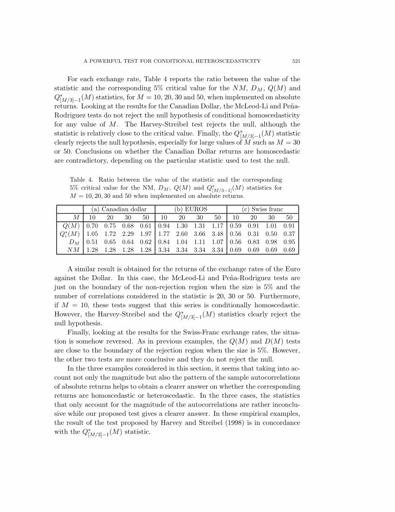
For each exchange rate, Table 4 reports the ratio between the value of the

statistic and the corresponding 5% critical value for the NM, DM , Q(M) and

Q∗

[M/3]−1(M) statistics, for M = 10, 20, 30 and 50, when implemented on absolute

returns. Looking at the results for the Canadian Dollar, the McLeod-Li and Pena-

Rodriguez tests do not reject the null hypothesis of conditional homoscedasticity

for any value of M . The Harvey-Streibel test rejects the null, although the

statistic is relatively close to the critical value. Finally, the Q∗

[M/3]−1(M) statistic

clearly rejects the null hypothesis, especially for large values of M such as M = 30

or 50. Conclusions on whether the Canadian Dollar returns are homoscedastic

are contradictory, depending on the particular statistic used to test the null.

Table 4. Ratio between the value of the statistic and the corresponding

5% critical value for the NM, DM , Q(M) and Q∗[M/3−1](M) statistics for

M = 10, 20, 30 and 50 when implemented on absolute returns.

(a) Canadian dollar (b) EUROS (c) Swiss franc

M 10 20 30 50 10 20 30 50 10 20 30 50

Q(M) 0.70 0.75 0.68 0.61 0.94 1.30 1.31 1.17 0.59 0.91 1.01 0.91

Q∗i (M) 1.05 1.72 2.29 1.97 1.77 2.60 3.66 3.48 0.56 0.31 0.50 0.37

DM 0.51 0.65 0.64 0.62 0.84 1.04 1.11 1.07 0.56 0.83 0.98 0.95NM 1.28 1.28 1.28 1.28 3.34 3.34 3.34 3.34 0.69 0.69 0.69 0.69

A similar result is obtained for the returns of the exchange rates of the Euro

against the Dollar. In this case, the McLeod-Li and Pena-Rodriguez tests are

just on the boundary of the non-rejection region when the size is 5% and the

number of correlations considered in the statistic is 20, 30 or 50. Furthermore,

if M = 10, these tests suggest that this series is conditionally homoscedastic.

However, the Harvey-Streibel and the Q∗

[M/3]−1(M) statistics clearly reject the

null hypothesis.

Finally, looking at the results for the Swiss-Franc exchange rates, the situa-

tion is somehow reversed. As in previous examples, the Q(M) and D(M) tests

are close to the boundary of the rejection region when the size is 5%. However,

the other two tests are more conclusive and they do not reject the null.

In the three examples considered in this section, it seems that taking into ac-

count not only the magnitude but also the pattern of the sample autocorrelations

of absolute returns helps to obtain a clearer answer on whether the corresponding

returns are homoscedastic or heteroscedastic. In the three cases, the statistics

that only account for the magnitude of the autocorrelations are rather inconclu-

sive while our proposed test gives a clearer answer. In these empirical examples,

the result of the test proposed by Harvey and Streibel (1998) is in concordance

with the Q∗

[M/3]−1(M) statistic.


Acknowledgement

We are very grateful to Mike Wiper for his help with the final draft. This

research has been supported by project BEC2002.03720 from the Spanish Gov-

erment and the Fundacion BBVA.

References

Andersen, T. G. and Bollerslev, T. (1997). Heterogenous information arrivals and return volatil-

ity dynamics: Uncovering the long-run in high frequency returns. J. Finance 52, 975-1005.

Baillie R. T., Bollerslev, T. and Mikkelsen H. O. (1996). Fractionally integrated autoregressive

conditional heteroskedasticity. J. Econometrics 74, 3-30.

Bollerslev, T. (1986). Generalized autoregressive conditional heteroscedasticity. J. Economet-

rics 31, 307-327.

Bollerslev, T. and Mikkelsen, H. O. (1999). Long-term equity anticipation securities and stock

market volatility dynamics. J. Econometrics 92, 75-99.

Box, G. E. P. (1954). Some theorems on quadratic forms applied in the study of analysis of

variance problems I: Effect of the inequality of variance in the one-way classification. Ann.

Math. Statist. 25, 290-302.

Breidt, F. J., Crato, N. and de Lima, P. J. F. (1998). The detection and estimation of long-

memory in stochastic volatility. J. Econometrics 83, 325-348.

Breidt, F. J. and Davis, R. A. (1992). Time-Reversibility, identifiability and indendence of

innovations for stationary time series. J. Time Ser. Anal. 25, 265-281.

Carnero, M. A., Pena, D. and Ruiz, E. (2004a). Persistence and kurtosis in GARCH and

stochastic volatility models. J. Finan. Econom. 13, 377-390.

Carnero, M. A., Pena, D. and Ruiz, E. (2004b). Spurious and hidden volatility. WP 04-20 (07),

Universidad Carlos III de Madrid.

Chen, W. W. and Deo, R. S. (2004). On power transformations to induce normality and their

applications. J. Roy. Statist. Soc. Ser. B 66, 117-130.

Ding, Z., Granger, C. W. J. and Engle, R. F. (1993). A long memory property of stock market

returns and a new model. J. Empirical Finance 1, 83-106.

Engle, R. F. (1982). Autoregressive conditional heteroskedasticity with estimates of the vari-

ances. Econometrica 50, 987-1007.

Ferguson, T. S. (1967). Mathematical Statistics: A Decision Theoretic Approach. Academic

Press, New York.

Ghysels, E., Harvey, A. C. and Renault, E. (1996). Stochastic volatility. In Statistical Methods in

Finance (Edited by C. R. Rao and G. S. Maddala), 119-191. North-Holland, Amsterdam.

Hannan, E. J. (1970). Multiple Time Series. Wiley, New York.

Harvey, A. C. (1998). Long memory in Stochastic Volatility. In Forecasting Volatility in Fi-

nancial Markets (Edited by J. Knight and S. Satchell), 307-320. Butterworth-Haineman,

Oxford.

Harvey, A. C. and Streibel, M. (1998). Testing for a slowly changing level with special reference

to stochastic volatility. J. Econometrics 87, 167-189. In Recent Developments in Time

Series, 2003 (Reproduced by P. Newbold and S. J. Leybourne). Edward Elgar Publishing.

Hong, Y. (1996). Consistent testing for serial correlation of unknown form. Econometrica 64,

837-864.

Jacquier, E., Polson, N. G. and Rossi, P. E., (1994). Bayesian analysis of stochastic volatility

models (with discussion). J. Bus. Econom. Statist. 12, 371-417.


Karanasos, M., Psaradakis, Z. and Sola, M. (2004). On the autocorrelation properties of long-

memory GARCH processes. J. Time Ser. Anal. 25, 265-281.

Koch, P. D. and Yang, S. (1986). A method for testing the independence of two time series

that accounts for a potential pattern in the cross-correlation function. J. Amer. Statist.

Assoc. 81, 533-544.

Ljung, G. M. and Box, G. E. P. (1978). On a measure of lack of fit in time series models.

Biometrika 65, 297-303.

McLeod, A. I. and Li, W. K. (1983). Diagnostic checking ARMA time series models using

squared-residual autocorrelations. J. Time Ser. Anal. 4, 269-273.

Palma, W. and Zevallos, M. (2004). Analysis of the correlation structure of square time series.

J. Time Ser. Anal. 25, 529-550.

Pena, D. and Rodrıguez, J. (2002). A powerful portmanteau test of lack of fit for time series.

J. Amer. Statist. Assoc. 97, 601-610.

Pena, D. and Rodrıguez, J. (2005a). The log of the determinant of the autocorrelation matrix

for testing goodness of fit in time series. J. Statist. Plann. Inference. Forthcoming.

Pena, D. and Rodrıguez, J. (2005b). Detecting nonlinearity in time series by model selection

criteria. Internat. J. Forecasting. Forthcoming.

Perez, A. and Ruiz, E. (2003). Properties of the sample autocorrelations of non-linear trans-

formations in long memory stochastic volatility models. J. Financial Econometrics 1,

420-444.

Satterthwaite, F. E. (1941). Synthesis of Variance. Psychometrica 6, 309-316.

Satterthwaite, F. E. (1946). An approximate distribution of estimates of variance components.

Biometrics Bull. 2, 110-114.

Taylor, J. H. (1986). Modelling Financial Time Series. Wiley, New York.

Tol, R. S. J. (1996). Autoregressive conditional heteroscedasticity in daily temperatures mea-

surements. Environmetrics 7, 67-75.

Departamento de Estadıstica, Universidad Carlos III de Madrid, C/ Madrid 126, 28903 Getafe,

Madrid, Spain.

E-mail: [email protected]

Laboratorio de Estadıstica, Universidad Politecnica de Madrid, Avda. Ramiro de Maeztu, 7,

E-28040 Madrid, Spain.

E-mail: [email protected]

(Received November 2003; accepted December 2004)

A Powerful test for conditional heteroscedasticity for financial time series with highly persistent...

Documents

Transcript of A Powerful test for conditional heteroscedasticity for financial time series with highly persistent...