How Powerful are Performance Predictors in Neural ...

How Powerful are Performance Predictorsin Neural Architecture Search?

Colin White1∗, Arber Zela2, Binxin Ru3, Yang Liu1, Frank Hutter2,41 Abacus.AI, 2 University of Freiburg, 3 University of Oxford,

4 Bosch Center for Artificial Intelligence

Abstract

Early methods in the rapidly developing field of neural architecture search (NAS)required fully training thousands of neural networks. To reduce this extremecomputational cost, dozens of techniques have since been proposed to predict thefinal performance of neural architectures. Despite the success of such performanceprediction methods, it is not well-understood how different families of techniquescompare to one another, due to the lack of an agreed-upon evaluation metric andoptimization for different constraints on the initialization time and query time. Inthis work, we give the first large-scale study of performance predictors by analyzing31 techniques ranging from learning curve extrapolation, to weight-sharing, tosupervised learning, to zero-cost proxies. We test a number of correlation- andrank-based performance measures in a variety of settings, as well as the ability ofeach technique to speed up predictor-based NAS frameworks. Our results act asrecommendations for the best predictors to use in different settings, and we showthat certain families of predictors can be combined to achieve even better predictivepower, opening up promising research directions. Our code, featuring a library of 31performance predictors, is available at https://github.com/automl/naslib.

1 Introduction

Neural architecture search (NAS) is a popular area of machine learning, which aims to automatethe process of developing neural architectures for a given dataset. Since 2017, a wide varietyof NAS techniques have been proposed [78, 45, 32, 49]. While the first NAS techniques trainedthousands of architectures to completion and then evaluated the performance using the final validationaccuracy [78], modern algorithms use more efficient strategies to estimate the performance ofpartially-trained or even untrained neural networks [11, 2, 54, 34, 38].

Recently, many performance prediction methods have been proposed based on training a model topredict the final validation accuracy of an architecture just from an encoding of the architecture.Popular choices for these models include Gaussian processes [60, 17, 51], neural networks [36, 54,65, 69], tree-based methods [33, 55], and so on. However, these methods often require hundredsof fully-trained architectures to be used as training data, thus incurring high initialization time. Incontrast, learning curve extrapolation methods [11, 2, 20] need little or no initialization time, buteach individual prediction requires partially training the architecture, incurring high query time. Veryrecently, a few techniques have been introduced which are fast both in query time and initializationtime [38, 1], computing predictions based on a single minibatch of data. Finally, using sharedweights [45, 4, 32] is a popular paradigm for NAS [73, 25], although the effectiveness of thesemethods in ranking architectures is disputed [53, 74, 76].

Despite the widespread use of performance predictors, it is not known how methods from differentfamilies compare to one another. While there have been some analyses on the best predictors within

∗{colin, yang}@abacus.ai, {zelaa, fh}@cs.uni-freiburg.de, [email protected]

35th Conference on Neural Information Processing Systems (NeurIPS 2021).

https://github.com/automl/naslib

0HWULFV

0RGHO�EDVHG��WUDLQDEOH /HDUQLQJ�FXUYH�EDVHG

=HUR�FRVW�3UR[LHV

(DUO\�6WRS��$FF��(DUO\�6WRS��/RVV�6R7/��6R7/�(

([WUDSRODWLRQ/&(/&(�P/F695

*3¶V*36SDUVH�*39DU��6SDUVH�*3

7UHHV/*%RRVW1*%RRVW5);*%RRVW

'HHS�1HWV%$1$1$6%2+$0,$11%21$6�'1*2�*&1��0/31$2�6HPL1$6

:HLJKW�VKDULQJ2QH6KRW5DQGRP�6HDUFK�:6

)LVKHU�� *UDG�1RUP ��*UDVS-DF��&RY�� 6\Q)ORZ��61,3��

%D\HV��/LQ��5HJ�

Init time (seconds) 103

104

105

Query time (se

conds)

100

101

102

Kend

all T

au

0.0

0.2

0.4

0.6

0.8

Kendall Tau on NAS-Bench-201 CIFAR-10

BANANASBOHAMIANNBONASBayes. Lin. Reg.DNGOEarly Stop (Acc.)Early Stop (Loss)GCNGPLCELCE-mLGBoostMLPNAONGBoostRF

SemiNASSoTLSoTL-ESparse GPVar. Sparse GPXGBoostFisherGrad NormGraspJacob. Cov.LcSVROneShotRSWSSNIPSynFlow

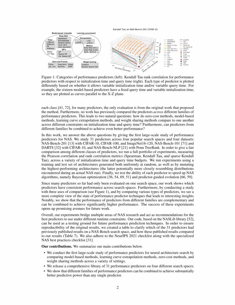
Figure 1: Categories of performance predictors (left). Kendall Tau rank correlation for performancepredictors with respect to initialization time and query time (right). Each type of predictor is plotteddifferently based on whether it allows variable initialization time and/or variable query time. Forexample, the sixteen model-based predictors have a fixed query time and variable initialization time,so they are plotted as curves parallel to the X-Z plane.

each class [41, 72], for many predictors, the only evaluation is from the original work that proposedthe method. Furthermore, no work has previously compared the predictors across different families ofperformance predictors. This leads to two natural questions: how do zero-cost methods, model-basedmethods, learning curve extrapolation methods, and weight sharing methods compare to one anotheracross different constraints on initialization time and query time? Furthermore, can predictors fromdifferent families be combined to achieve even better performance?

In this work, we answer the above questions by giving the first large-scale study of performancepredictors for NAS. We study 31 predictors across four popular search spaces and four datasets:NAS-Bench-201 [13] with CIFAR-10, CIFAR-100, and ImageNet16-120, NAS-Bench-101 [71] andDARTS [32] with CIFAR-10, and NAS-Bench-NLP [21] with Penn TreeBank. In order to give a faircomparison among different classes of predictors, we run a full portfolio of experiments, measuringthe Pearson correlation and rank correlation metrics (Spearman, Kendall Tau, and sparse KendallTau), across a variety of initialization time and query time budgets. We run experiments using atraining and test set of architectures generated both uniformly at random, as well as by mutatingthe highest-performing architectures (the latter potentially more closely resembling distributionsencountered during an actual NAS run). Finally, we test the ability of each predictor to speed up NASalgorithms, namely Bayesian optimization [36, 54, 69, 51] and predictor-guided evolution [66, 59].

Since many predictors so far had only been evaluated on one search space, our work shows whichpredictors have consistent performance across search spaces. Furthermore, by conducting a studywith three axes of comparison (see Figure 1), and by comparing various types of predictors, we see amore complete view of the state of performance predictor techniques that leads to interesting insights.Notably, we show that the performance of predictors from different families are complementary andcan be combined to achieve significantly higher performance. The success of these experimentsopens up promising avenues for future work.

Overall, our experiments bridge multiple areas of NAS research and act as recommendations for thebest predictors to use under different runtime constraints. Our code, based on the NASLib library [52],can be used as a testing ground for future performance prediction techniques. In order to ensurereproducibility of the original results, we created a table to clarify which of the 31 predictors hadpreviously published results on a NAS-Bench search space, and how these published results comparedto our results (Table 7). We also adhere to the NeurIPS 2021 checklist along with the specializedNAS best practices checklist [31].

Our contributions. We summarize our main contributions below.

• We conduct the first large-scale study of performance predictors for neural architecture search bycomparing model-based methods, learning curve extrapolation methods, zero-cost methods, andweight sharing methods across a variety of settings.

• We release a comprehensive library of 31 performance predictors on four different search spaces.• We show that different families of performance predictors can be combined to achieve substantially

better predictive power than any single predictor.

2

2 Related Work

NAS has been studied since at least the 1990s [19, 58], and has been revitalized in the last fewyears [78]. While initial techniques focused on reinforcement learning [78, 45] and evolutionarysearch [37, 49], one-shot NAS algorithms [32, 12, 4] and predictor-based NAS algorithms [65, 54, 69]have recently become popular. We give a brief survey of performance prediction techniques inSection 3. For a survey on NAS, see [15]. The most widely used type of search space in prior workis the cell-based search space [79], where the architecture search is over a relatively small directedacyclic graph representing an architecture.

A few recent works have compared different performance predictors on popular cell-based searchspaces for NAS. Siems et al. [55] studied graph neural networks and tree-based methods, and foundthat gradient-boosted trees and graph isomorphism networks performed the best. However, thecomparison was only on a single search space and dataset, and the explicit goal was to achievemaximum performance given a training set of around 60 000 architectures. Another recent paper [41]studied various aspects of supernetwork training, and separately compared four model-based methods:random forest, MLP, LSTM, and GATES [42]. However, the comparisons were again on a singlesearch space and dataset and did not compare between multiple families of performance predictors.Other papers have proposed new model-based predictors and compared the new predictors to othermodel-based baselines [34, 65, 54, 69]. Finally, a recent paper analyzed training heuristics to makeweight-sharing more effective at ranking architectures [72]. To the best of our knowledge, no priorwork has conducted comparisons across multiple families of performance predictors.

3 Performance Prediction Methods for NAS

In NAS, given a search space A, the goal is to find a∗ = argmina∈Af(a), where f denotes thevalidation error of architecture a after training on a fixed dataset for a fixed number of epochs E.Since evaluating f(a) typically takes hours (as it requires training a neural network from scratch),many NAS algorithms make use of performance predictors to speed up this process. A performancepredictor f ′ is defined generally as any function which predicts the final accuracy or ranking ofarchitectures, without fully training the architectures. That is, evaluating f ′ should take less timethan evaluating f , and {f ′(a) | a ∈ A} should ideally have high correlation or rank correlation with{f(a) | a ∈ A}.Each performance predictor is defined by two main routines: an initialization routine which per-forms general pre-computation, and a query routine which performs the final architecture-specificcomputation: it takes as input an architecture specification, and outputs its predicted accuracy. Forexample, one of the simplest performance predictors is early stopping: for any query(a), train a forE/2 epochs instead of E [77]. In this case, there is no general pre-computation, so initializationtime is zero. On the other hand, the query time for each input architecture is high because it involvestraining the architecture for E/2 epochs. In fact, the runtime of the initialization and query routinesvaries substantially based on the type of predictor. In the context of NAS algorithms, the initializationroutine is typically performed once at the start of the algorithm, and the query routine is typicallyperformed many times throughout the NAS algorithm. Some performance predictors also makeuse of an update routine, when part of the computation from initialization needs to be updatedwithout running the full procedure again (for example, in a NAS algorithm, a model may be updatedperiodically based on newly trained architectures). Now we give an overview of the main families ofpredictors. See Figure 1 (left) for a taxonomy of performance predictors.

Model-based (trainable) methods. The most common type of predictor, the model-based pre-dictor, is based on supervised learning. The initialization routine consists of fully training manyarchitectures (i.e., evaluating f(a) for many architectures a ∈ A) to build a training set of datapoints{a, f(a)}. Then a model f ′ is trained to predict f(a) given a. While the initialization time formodel-based predictors is very high, the query time typically takes less than a second, which allowsthousands of predictions to be made throughout a NAS algorithm. The model is also updated regularlybased on the new datapoints. These predictors are typically used within BO frameworks [36, 54],evolutionary frameworks [66], or by themselves [67], to perform NAS. Popular choices for themodel include tree-based methods (where the features are the adjacency matrix representation of

3

the architectures) [33, 55], graph neural networks [36, 54], Gaussian processes [47, 51], and neuralnetworks based on specialized encodings of the architecture [69, 42].

Learning curve-based methods. Another family predicts the final performance of architecturesusing only a partially trained network, by extrapolating the learning curve. This is accomplished byfitting the partial learning curve to an ensemble of parametric models [11], or by simply summing thetraining losses observed so far [50]. Early stopping as described earlier is also a learning curve-basedmethod. Learning curve methods do not require any initialization time, yet the query time typicallytakes minutes or hours, which is orders of magnitude slower than the query time in model-basedmethods. Learning curve-based methods can be used in conjunction with multi-fidelty algorithms,such as Hyperband or BOHB [27, 16, 24].

Hybrid methods. Some predictors are hybrids between learning curve and model-based methods.These predictors train a model at initialization time to predict f(a) given both a and a partial learningcurve of a as features. Models in prior work include an SVR [2], or a Bayesian neural network [20].Although the query time and initialization time are both high, hybrid predictors tend to have strongperformance.

Zero-cost methods. Another class of predictors have no initialization time and very short querytimes (so-called “zero-cost” methods). These predictors compute statistics from just a single for-ward/backward propagation pass for a single minibatch of data, by computing the correlation ofactivations within a network [38], or by adapting saliency metrics proposed in pruning-at-initializationliteratures [23, 1]. Similar to learning curve-based methods, since the only computation is specific toeach architecture, the initialization time is zero. Zero-cost methods have recently been used to warmstart NAS algorithms [1].

Weight sharing methods. Weight sharing [45] is a popular approach to substantially speed upNAS, especially in conjunction with a one-shot algorithm [32, 12]. In this approach, all architecturesin the search space are combined to form a single over-parameterized supernetwork. By training theweights of the supernetwork, all architectures in the search space can be evaluated quickly using thisset of weights. To this end, the supernetwork can be used as a performance predictor. This resultsin NAS algorithms [32, 28] which are significantly faster than sequential NAS algorithms, such asevolution or Bayesian optimization. Recent work has shown that although the shared weights aresometimes not effective at ranking architectures [53, 74, 76], one-shot NAS techniques using sharedweights still achieve strong performance [73, 25].

Tradeoff between intialization and query time. The main families mentioned above all havedifferent initialization and query times. The tradeoffs between initialization time, query time, andperformance depend on a few factors such as the type of NAS algorithm and its total runtime budget,and different settings are needed in different situations. For example, if there are many architectureswhose performance we want to estimate, then we should have a low query time, and if we have a hightotal runtime budget, then we can afford a high initialization time. We may also change our runtimebudget throughout the run of a single NAS algorithm. For example, at the start of a NAS algorithm,we may want to have coarse estimates of a large number of architectures (low initialization time, lowquery time such as zero-cost predictors). As the NAS algorithm progresses, it is more desirable toreceive higher-fidelity predictions on a smaller set of architectures (model-based or hybrid predictors).The exact budgets depend on the type of NAS algorithm.

Choice of performance predictors. We analyze 31 performance predictors defined in prior work:BANANAS [69], Bayesian Linear Regression [6], BOHAMIANN [57], BONAS [54], DNGO [56],Early Stopping with Val. Acc. (e.g. [77, 27, 16, 79]) Early Stopping with Val. Loss. [50], Fisher [1],Gaussian Process (GP) [48], GCN [75], Grad Norm [1], Grasp [64], Jacobian Covariance [38],LCE [11], LCE-m [20], LcSVR [2], LGBoost/GBDT [33], MLP [69], NAO [35], NGBoost [55],OneShot [73], Random Forest (RF) [55], Random Search with Weight Sharing (RSWS) [26], Sem-iNAS [34], SNIP [23], SoTL [50], SoTL-E [50], Sparse GP [3], SynFlow [61], Variational SparseGP [63], and XGBoost [55]. For any method that did not have an architecture encoding alreadydefined (such as the tree-based methods, GP-based methods, and Bayesian Linear Regression), we usethe standard adjacency matrix encoding, which consists of the adjacency matrix of the architecturealong with a one-hot list of the operations [71, 68]. By open-sourcing our code, we encourage

4

104 105 106

Init. time (seconds)

101

102

103

Quer

y tim

e (s

econ

ds)

.93 .93 .93 .93 .93 .93 .93 .93 .93 .93 .93.93

.4

.57

.57

.57

.57

.57

.57

.57

.57

.57

.57

.57

.57

.57

.57

.57

.57

.57

.57

.57

.57

.57

.57

.57

.57

.57

.57

.57

.57

.57

.57

.57

.57

.57

.57

.57 .6

.58

.62

.65

.6

.63

.66

.6

.64

.67

.7

.65

.67

.7

.69

.72

.74

.84

.73

.75

.77

.85

.63

.69

.74

.77

.8

.82

.83

.84

.84

.63

.69

.74

.77

.8

.82

.83

.84

.84

.63

.69

.74

.77

.8

.82

.83

.84

.84

.63

.69

.74

.77

.8

.82

.83

.84

.84

.63

.69

.74

.77

.8

.82

.83

.84

.84

.69

.74

.77

.8

.82

.83

.84

.84

.69

.74

.77

.8

.82

.83

.84

.84

.74

.77

.8

.82

.83

.84

.84

.74

.77

.8

.82

.83

.84

.84

.77

.8

.82

.83

.84

.8

.82

.83

.84

.63

.69

.74

.77

.8

.82

.83

.84

.84

.28 .42 .46 .5 .53 .57 .6

.6

.6

.6

.63

.63

.63

.63

.63

.68

.68

.68

.68

.68

.68

.73

.73

.73

.73

.73

.73

.73


105 106 107


102

103

104

Quer

y tim

e (s

econ

ds)

NAS-Bench-NLP

105 106 107


102

103

104

Quer

y tim

e (s

econ

ds)

NAS-Bench-201 ImageNet16-120

104 105 106


101

102

103

Quer

y tim

e (s

econ

ds)

NAS-Bench-101

104 105


101

102

103

Quer

y tim

e (s

econ

ds)

DARTS

5.00 5.25 5.50 5.75 6.005.0

5.2

5.4

5.6

5.8

6.0

BANANASBayes. Lin. Reg.

Early Stop (Acc.)GCN

Jacob. Cov.LGBoost

LcSVRNGBoost

SoTL-ESemiNAS

SynFlowXGBoost

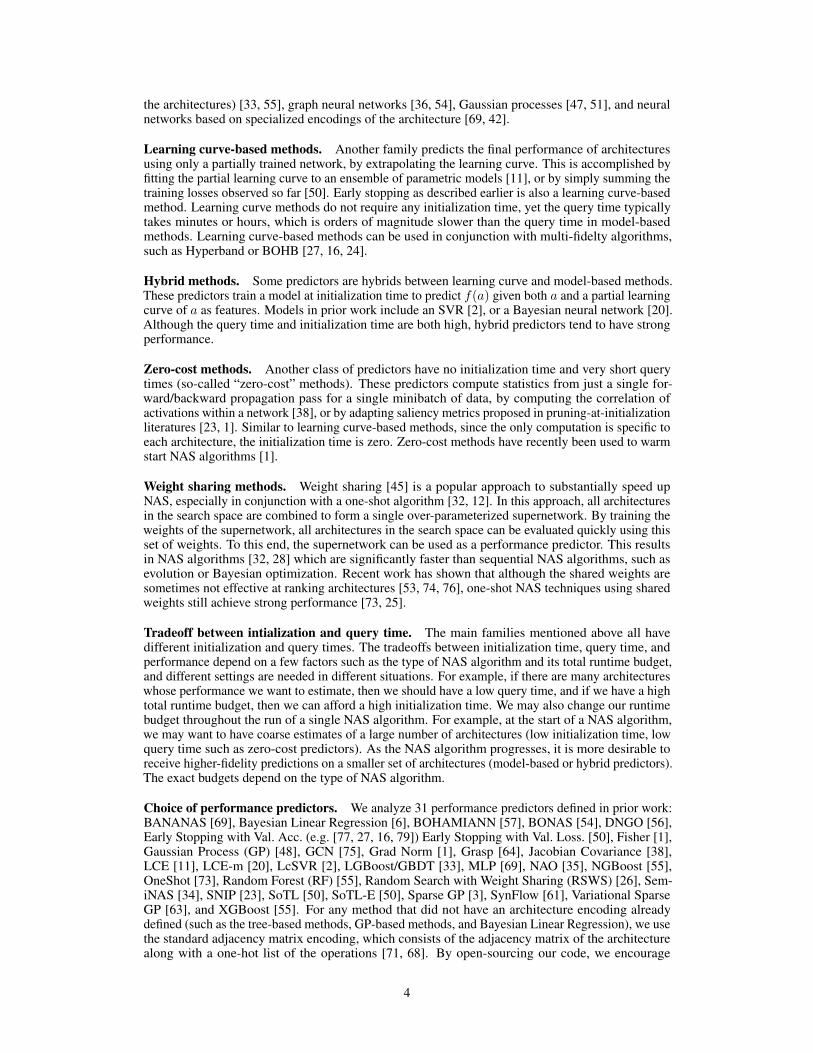
Figure 2: The performance predictors with the highest Kendall Tau values for all initialization timeand query time budgets on NAS-Bench-201, NAS-Bench-101, NAS-Bench-NLP and DARTS. Forexample, on NAS-Bench-201 CIFAR-10 (left) with an initialization time of 106 seconds and querytime of 10 seconds, XGBoost achieves a Kendall Tau value of .73 which is the highest value out ofthe 31 predictors that we tested at that budget.

implementing more (existing and future) performance predictors which can then be compared to the31 which we focus on in this work. In Section B.1, we give descriptions and detailed implementationdetails for each performance predictor. In Section D, we give a table that describes for which pre-dictors we were able to reproduce published results, and for which predictors it is not possible (e.g.,since some predictors were released before the creation of NAS benchmarks).

4 Experiments

We now discuss our experimental setup and results. We discuss reproducibility in Sections A and D,and our code (based on the NASLib library [52]) is available at https://github.com/automl/naslib. We split up our experiments into two categories: evaluating the performance of eachpredictor with respect to various correlation metrics (Section 4.1), and evaluating the ability of eachpredictor to speed up predictor-based NAS algorithms (Section 4.2). We start by describing the fourNAS benchmarks used in our experiments.

NAS benchmark datasets. NAS-Bench-101 [71] consists of over 423 000 unique neural architec-tures with precomputed training, validation, and test accuracies after training for 4, 12, 36, and 108epochs on CIFAR-10 [71]. The cell-based search space consists of five nodes which can take on anydirected acyclic graph (DAG) structure, and each node can be one of three operations. Since learningcurve information is only available at four epochs, it is not possible to run most learning curve extrap-olation methods on NAS-Bench-101. NAS-Bench-201 [13] consists of 15 625 architectures (out ofwhich 6 466 are unique after removing isomorphisms [13]). Each architecture has full learning curveinformation for training, validation, and test losses/accuracies for 200 epochs on CIFAR-10 [22],CIFAR-100, and ImageNet-16-120 [10]. The search space consists of a cell which is a complete DAGwith 4 nodes. Each edge can take one of five different operations. The DARTS search space [32] issignificantly larger with roughly 1018 architectures. The search space consists of two cells, each withseven nodes. The first two nodes are inputs from previous layers, and the intermediate four nodes cantake on any DAG structure such that each node has two incident edges. The last node is the outputnode. Each edge can take one of eight operations. In our experiments, we make use of the trainingdata from NAS-Bench-301 [55], which consists of 23 000 architectures drawn uniformly at randomand trained on CIFAR-10 for 100 epochs. Finally, the NAS-Bench-NLP search space [21] is even

5



larger, at 1053 LSTM-like cells, each with at most 25 nodes in any DAG structure. Each cell can takeone of seven operations. In our experiments, we use the NAS-Bench-NLP dataset, which consists of14 000 architectures drawn uniformly at random and trained on Penn Tree Bank [40] for 50 epochs.

Hyperparameter tuning. Although we used the code directly from the original repositories (some-times making changes when necessary to adapt to NAS-Bench search spaces), the predictors hadsignificantly different levels of hyperparameter tuning. For example, some of the predictors hadundergone heavy hyperparameter tuning on the DARTS search space (used in NAS-Bench-301),while other predictors (particularly those from 2017 or earlier) had never been run on cell-basedsearch spaces. Furthermore, most predictor-based NAS algorithms can utilize cross-validation to tunethe predictor periodically throughout the NAS algorithm. This is because the bottleneck for predictor-based NAS algorithms is typically the training of architectures, not fitting the predictor [56, 30, 16].Therefore, it is fairer and also more informative to compare performance predictors which have hadthe same level of hyperparameter tuning through cross-validation. For each search space, we runrandom search on each performance predictor for 5000 iterations, with a maximum total runtime of15 minutes. The final evaluation uses a separate test set. The hyperparameter value ranges for eachpredictor can be found in Section B.2.

4.1 Performance Predictor Evaluation

We evaluate each predictor based on three axes of comparison: initialization time, query time, andperformance. We measured performance with respect to several different metrics: Pearson correlationand three different rank correlation metrics (Spearman, Kendall Tau, and sparse Kendall Tau [72, 55]).The experimental setup is as follows: the predictors are tested with 11 different initialization timebudgets and 14 different query time budgets, leading to a total of 154 settings. On NAS-Bench-201CIFAR-10, the 11 initialization time budgets are spaced logarithmically from 1 second to 1.8× 107

seconds on a 1080 Ti GPU (which corresponds to training 1000 random architectures on average)which is consistent with experiments conducted in prior work [65, 69, 34]. For other search spaces,these times are adjusted based on the average time to train 1000 architectures. The 14 query timebudgets are spaced logarithmically from 1 second to 1.8×104 seconds (which corresponds to trainingan architecture for 199 epochs). These times are adjusted for other search spaces based on the trainingtime and different number of epochs. Once the predictor is initialized, we draw a test set of 200architectures uniformly at random from the search space. For each architecture in the test set, thepredictor uses the specified query time budget to make a prediction. We then evaluate the quality ofthe predictions using the metrics described above. We average the results over 100 trials for each(initialization time, query time) pair.

Results and discussion. Figure 1 shows a full three-dimensional plot for NAS-Bench-201 onCIFAR-10 over initialization time, query time, and Kendall Tau rank correlation. Of the 31 predictorswe tested, we found that just seven of them are Pareto-optimal with respect to Kendall Tau, initial-ization time, and query time. That is, only seven algorithms have the highest Kendall Tau value forat least one of the 154 query time/initialization time budgets on NAS-Bench-201 CIFAR-10. Thiscan be seen more clearly in Figure 2 (left), which is a view from above Figure 1: each lattice pointdisplays the predictor with the highest Kendall Tau value for the corresponding budget. In Figure 2(right), we plot the Pareto-optimal predictors for five different dataset/search space combinations.In Section B.3, we give the full 3D plots and report the variance across trials for each method. InFigure 4 (left), we also plot the Pearson and Spearman correlation coefficients for NAS-Bench-201CIFAR-10. The trends between these measures are largely the same, although we see that SemiNASperforms better on the rank-based metrics. For the rest of this section, we focus on the popularKendall Tau metric, giving the full results for the other metrics in Section B.3.

We see similar trends across DARTS and the two NAS-Bench-201 datasets. NAS-Bench-NLP alsohas fairly similar trends, although early stopping performs comparatively stronger. NAS-Bench-101is different from the other search spaces both in terms of the topology and the benchmark itself,which we discuss later in this section.

In the low initialization time, low query time region, Jacobian covariance or SynFlow perform wellacross NAS-Bench-101 and NAS-Bench-201. However, none of the six zero-cost methods performwell on the larger DARTS search space. Weight sharing (which also has low initialization and lowquery time, as seen in Figure 1), did not yield high Kendall Tau values for these search spaces, either,

6

104 105 106


101

102

103

Quer

y tim

e (s

econ

ds)

NAS-Bench-201 CIFAR-10

>60%>70%>80%>90%>100%>110%>120%

105 106

Init. time (seconds)101

102

103

Quer

y tim

e (s

econ

ds)

NAS-Bench-201 CIFAR-100

>70%>80%>90%>100%>110%>120%

105 106 107


102

103

104

Quer

y tim

e (s

econ

ds)

NAS-Bench-201 ImageNet16

>70%>80%>90%>100%>110%>120%>130%

104 105


101

102

103

Quer

y tim

e (s

econ

ds)

DARTS

<60%>60%>70%>80%>90%>100%

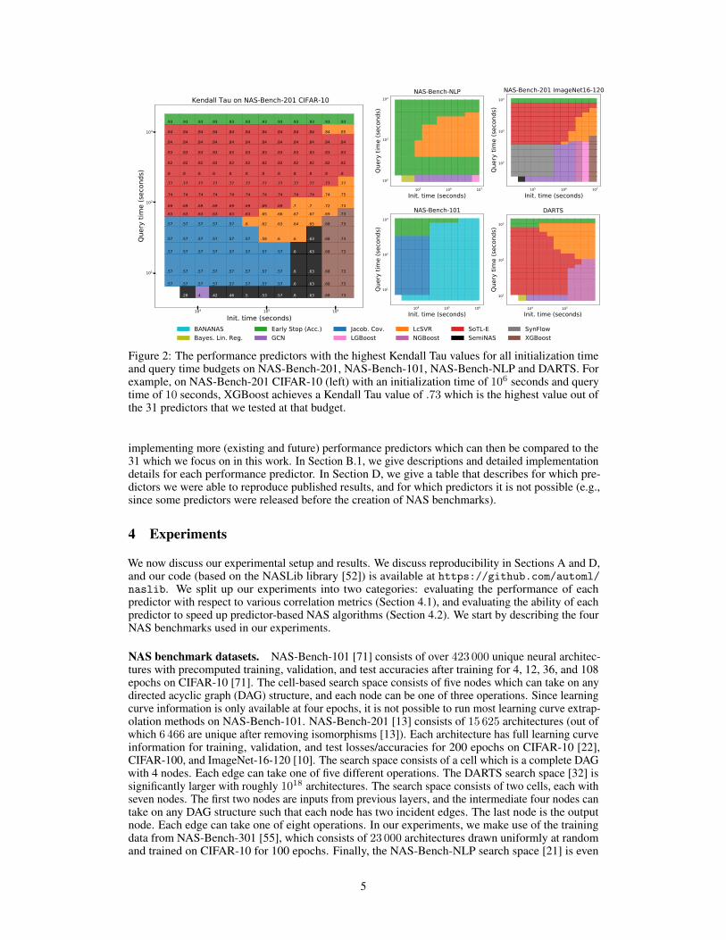
Figure 3: Percentage of OMNI’s Kendall Tau value compared to the next-best predictors for eachbudget constraint.

which is consistent with recent work [53, 74, 76]. However, rank correlation is not as crucial toone-shot NAS algorithms as it is for black box predictor-based methods, as demonstrated by priorone-shot NAS methods that do perform well [25, 73, 32, 28, 12]. In the low initialization time, highquery time region, sum of training losses (SoTL-E) consistently performed the best, outperformingother learning-curve based methods.

The high initialization time, low query time region (especially the bottom row of the plots, correspond-ing to a query time of 1 second) is by far the most competitive region in the recent NAS literature.Sixteen of the 31 predictors had query times under one second, because many NAS algorithms aredesigned to initialize (and continually update) performance predictors that are used to quickly querythousands of candidate architectures. GCN and SemiNAS, the specialized GCN/semi-supervisedmethods, perform especially well in the first half of this critical region, when the initialization timeis relatively low. However, boosted tree methods actually performed best in the second half of thecritical region where the initialization time is high, which is consistent with prior work [33, 55].Recall that for model-based methods, the initialization time corresponds to training architectures tobe used as training data for the performance predictor. Therefore, our results suggest that techniqueswhich can extract better latent features of the architectures can make up for a small training dataset,but methods based purely on performance data work better when there is enough such data.

Perhaps the most interesting finding is that on NAS-Bench-101/201, SynFlow and Jacobian covariance,which take three seconds each to compute, both outperform all model-based methods even after 30hours of initialization. Put another way, NAS algorithms that make use of model-based predictorsmay be able to see substantial improvements by using Jacobian covariance instead of a model-basedpredictor in the early iterations.

The Omnipotent Predictor. One conclusion from Figure 2 is that different types of predictors arespecialized for specific initialization time and query time constraints. A natural follow-up question iswhether different families are complementary and can be combined to achieve stronger performance.In this section, we run a proof-of-concept to answer this question. We combine the best-performingpredictors from three different families in a simple way: the best learning curve method (SoTL-E),and the best zero-cost method (Jacobian covariance), are used as additional input features for amodel-based predictor (we separately test SemiNAS and NGBoost). We call this method OMNI, theomnipotent predictor. We give results in Figure 3 and pseudo-code as well as additional experimentsin Section B.4. In contrast to all other predictors, the performance of OMNI is strong across almostall budget constraints and search spaces. In some settings, OMNI achieves a Kendall Tau value 30%higher than the next-best predictors.

The success of OMNI verifies that the information learned by different families of predictors arecomplementary: the information learned by extrapolating a learning curve, by computing a zero-costproxy, and by encoding the architecture, all improve performance. We further confirm this by runningan ablation study for OMNI in Section B.4. We can hypothesize that each predictor type measuresdistinct quantities: SOTL-E measures the training speed, zero-cost predictors measure the covariancebetween activations on different datapoints, and model-based predictors simply learn patterns betweenthe architecture encodings and the validation accuracies. Finally, while we showed a proof-of-concept,there are several promising areas for future work such as creating ensembles of the model-basedapproaches, combining zero-cost methods with model-based methods in more sophisticated ways,and giving a full quantification of the correlation among different families of predictors.

7

104 105 106


101

102

103

Quer

y tim

e (s

econ

ds)

Pearson correlation

Early Stop (Acc.)GCNJacob. Cov.LcSVRSoTL-ESemiNASXGBoost

104 105 106


101

102

103

Quer

y tim

e (s

econ

ds)

Spearman rank correlation


104

105

Query time (se

conds)

100

101

102

Kend

all T

au

0.0

0.2

0.4

0.6

0.8


BANANASBOHAMIANNBONASBayes. Lin. Reg.DNGOEarly Stop (Acc.)Early Stop (Loss)GCNGPLCELCNetLGBoostMLPNAONGBoostRFSemiNASSoTLSoTL-ESparse GPVar. Sparse GPXGBoostFisherGrad NormGraspJacob. Cov.LcSVRSNIPSynFlow


104

105

Query time (se

conds)

100

101

102

Kend

all T

au

0.0

0.2

0.4

0.6

0.8


BANANASBOHAMIANNBONASBayes. Lin. Reg.

DNGOEarly Stop (Acc.)Early Stop (Loss)GCN

GPLCELCE-mLGBoost

MLPNAONGBoostRF

SemiNASSoTLSoTL-ESparse GP

Var. Sparse GPXGBoostFisher

Grad NormGraspJacob. Cov.

LcSVRSNIPSynFlow

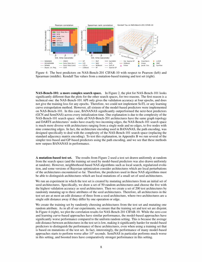
Figure 4: The best predictors on NAS-Bench-201 CIFAR-10 with respect to Pearson (left) andSpearman (middle). Kendall Tau values from a mutation-based training and test set (right).

NAS-Bench-101: a more complex search space. In Figure 2, the plot for NAS-Bench-101 lookssignificantly different than the plots for the other search spaces, for two reasons. The first reason is atechnical one: the NAS-Bench-101 API only gives the validation accuracy at four epochs, and doesnot give the training loss for any epochs. Therefore, we could not implement SoTL or any learningcurve extrapolation method. However, all sixteen of the model-based predictors were implementedon NAS-Bench-101. In this case, BANANAS significantly outperformed the next-best predictors(GCN and SemiNAS) across every initialization time. One explanation is due to the complexity of theNAS-Bench-101 search space: while all NAS-Bench-201 architectures have the same graph topologyand DARTS architectures’ nodes have exactly two incoming edges, the NAS-Bench-101 search spaceis much more diverse with architectures ranging from a single node and no edges, to five nodes withnine connecting edges. In fact, the architecture encoding used in BANANAS, the path encoding, wasdesigned specifically to deal with the complexity of the NAS-Bench-101 search space (replacing thestandard adjacency matrix encoding). To test this explanation, in Appendix B we run several of thesimpler tree-based and GP-based predictors using the path encoding, and we see that these methodsnow surpass BANANAS in performance.

A mutation-based test set. The results from Figure 2 used a test set drawn uniformly at randomfrom the search space (and the training set used by model-based predictors was also drawn uniformlyat random). However, neighborhood-based NAS algorithms such as local search, regularized evolu-tion, and some versions of Bayesian optimization consider architectures which are local perturbationsof the architectures encountered so far. Therefore, the predictors used in these NAS algorithms mustbe able to distinguish architectures which are local mutations of a small set of seed architectures.

We run an experiment in which the test set is created by mutating architectures from an initial set ofseed architectures. Specifically, we draw a set of 50 random architectures and choose the five withthe highest validation accuracy as seed architectures. Then we create a set of 200 test architectures byrandomly mutating up to three attributes of the seed architectures. Therefore, all architectures in thetest set are at most an edit distance of three from a seed architecture, where two architectures are asingle edit distance away if they differ by one operation or edge.

We create the training set by randomly choosing architectures from the test set and mutating onerandom attribute. As in all of our experiments, we ensure that the training set and test set are disjoint.In Figure 4 (right), we plot the correlation results for NAS-Bench-201 CIFAR-10. While the zero-costand learning curve-based approaches have similar performance, the model-based approaches havesignificantly worse performance compared to the uniform random setting. This is because the averageedit distance between architectures in the test set is low, making it significantly harder for model-basedpredictors to distinguish the performance of these architectures, even when using a training set thatis based on mutations of the test set. In fact, interestingly, the performance of many model-basedapproaches starts to perform worse after 106 seconds. SemiNAS in particular performs much worsein this setting, and boosted trees have comparatively stronger performance in this setting.

8

105

Runtime (seconds)8.4

8.6

8.8

9.0

9.2

9.4

9.6

Valid

atio

n er

ror (

%)

Evol. NAS Framework, NAS-Bench-201 CIFAR10

8.5 × 105 9 × 105

8.50

8.55

106

Runtime (seconds)

53.0

53.5

54.0

54.5

55.0

Valid

atio

n er

ror (

%)

Evol. NAS Framework, NAS-Bench-201 ImageNet16-120

5.1 × 106 5.4 × 106

52.8

52.9

105


8.8

9.0

9.2

9.4

9.6

Valid

atio

n er

ror (

%)

BO Framework, NAS-Bench-201 CIFAR10

8.5 × 105 9 × 105

8.625

8.650

8.675

106

Runtime (seconds)

53.00

53.25

53.50

53.75

54.00

54.25

54.50

54.75

55.00

Valid

atio

n er

ror (

%)

BO Framework, NAS-Bench-201 ImageNet16-120

5.1 × 106 5.4 × 10652.9

53.0

105


8.8

9.0

9.2

9.4

9.6

Valid

atio

n er

ror (

%)

BO Framework, NAS-Bench-201 CIFAR10

BANANASBONASBOHAMIANNBayes. Lin. Reg.DNGOMLPLGBoostGCNGPNAORFSparse GPVar. Sparse GPXGBoostNGBoostOMNI(NGBoost)SemiNASOMNI(SemiNAS)

8.5 × 105 9 × 105

8.625

8.650

8.675

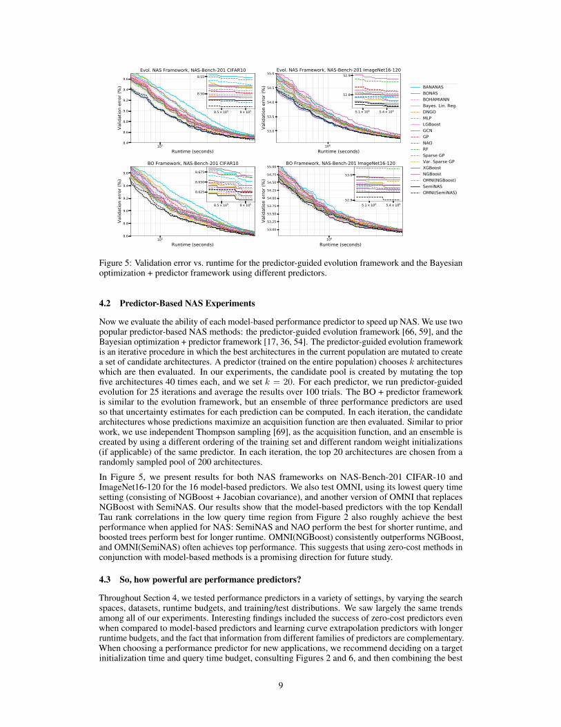
Figure 5: Validation error vs. runtime for the predictor-guided evolution framework and the Bayesianoptimization + predictor framework using different predictors.

4.2 Predictor-Based NAS Experiments

Now we evaluate the ability of each model-based performance predictor to speed up NAS. We use twopopular predictor-based NAS methods: the predictor-guided evolution framework [66, 59], and theBayesian optimization + predictor framework [17, 36, 54]. The predictor-guided evolution frameworkis an iterative procedure in which the best architectures in the current population are mutated to createa set of candidate architectures. A predictor (trained on the entire population) chooses k architectureswhich are then evaluated. In our experiments, the candidate pool is created by mutating the topfive architectures 40 times each, and we set k = 20. For each predictor, we run predictor-guidedevolution for 25 iterations and average the results over 100 trials. The BO + predictor frameworkis similar to the evolution framework, but an ensemble of three performance predictors are usedso that uncertainty estimates for each prediction can be computed. In each iteration, the candidatearchitectures whose predictions maximize an acquisition function are then evaluated. Similar to priorwork, we use independent Thompson sampling [69], as the acquisition function, and an ensemble iscreated by using a different ordering of the training set and different random weight initializations(if applicable) of the same predictor. In each iteration, the top 20 architectures are chosen from arandomly sampled pool of 200 architectures.

In Figure 5, we present results for both NAS frameworks on NAS-Bench-201 CIFAR-10 andImageNet16-120 for the 16 model-based predictors. We also test OMNI, using its lowest query timesetting (consisting of NGBoost + Jacobian covariance), and another version of OMNI that replacesNGBoost with SemiNAS. Our results show that the model-based predictors with the top KendallTau rank correlations in the low query time region from Figure 2 also roughly achieve the bestperformance when applied for NAS: SemiNAS and NAO perform the best for shorter runtime, andboosted trees perform best for longer runtime. OMNI(NGBoost) consistently outperforms NGBoost,and OMNI(SemiNAS) often achieves top performance. This suggests that using zero-cost methods inconjunction with model-based methods is a promising direction for future study.

4.3 So, how powerful are performance predictors?

Throughout Section 4, we tested performance predictors in a variety of settings, by varying the searchspaces, datasets, runtime budgets, and training/test distributions. We saw largely the same trendsamong all of our experiments. Interesting findings included the success of zero-cost predictors evenwhen compared to model-based predictors and learning curve extrapolation predictors with longerruntime budgets, and the fact that information from different families of predictors are complementary.When choosing a performance predictor for new applications, we recommend deciding on a targetinitialization time and query time budget, consulting Figures 2 and 6, and then combining the best

9

predictors from the desired runtime setting, similar to OMNI. For example, if a performance predictorwith medium initialization time and low runtime is desired for a search space similar to NAS-Bench-201 or DARTS, we recommend using NGBoost with Jacobian covariance and SynFlow as additionalfeatures.

5 Societal Impact

Our hope is that our work will have a positive impact on the AutoML community by making it quickerand easier to develop and fairly compare performance predictors. For example, AutoML practitionerscan consult our experiments to more easily decide on the performance prediction methods bestsuited to their application, rather than conducting computationally intensive experiments of theirown [43]. Furthermore, AutoML researchers can use our library to develop new performanceprediction techniques and compare new methods to 31 other algorithms across four search spaces.Since the topic of this work is AutoML, it is a level of abstraction away from real applications.This work may be used to improve deep learning applications, both beneficial (e.g. reducing CO2

emissions), or harmful (e.g. creating language models with heavy bias) to society.

6 Conclusions and Limitations

In this work, we gave the first large-scale study of performance predictors for neural architecturesearch. We compared 31 different performance predictors, including learning curve extrapolationmethods, weight sharing methods, zero-cost methods, and model-based methods. We tested theperformance of the predictors in a variety of settings and with respect to different metrics. Althoughwe ran experiments on four different search spaces, it will be interesting to extend our experiments toeven more machine learning tasks beyond image classification and language modeling.

Our new predictor, OMNI, is the first predictor to combine complementary information from threefamilies of performance preditors, leading to substantially improved performance. While the simplic-ity of OMNI is appealing, it also opens up new directions for future work by combining differentpredictors in more sophisticated ways. To facilitate follow-up work, we release our code featuring alibrary of performance predictors. Our goal is for our repository to grow over time as it is used by thecommunity, so that experiments in our library can be even more comprehensive.

Acknowledgments and Disclosure of Funding

This work was done while CW and YL were employed at Abacus.AI. AZ and FH acknowledgesupport by the European Research Council (ERC) under the European Union Horizon 2020 researchand innovation programme through grant no. 716721, and by BMBF grant DeToL. BR was supportedby the Clarendon Fund of University of Oxford.

10

References[1] Mohamed S Abdelfattah, Abhinav Mehrotra, Łukasz Dudziak, and Nicholas Donald Lane.

Zero-cost proxies for lightweight nas. In Proceedings of the International Conference onLearning Representations (ICLR), 2021.

[2] Bowen Baker, Otkrist Gupta, Ramesh Raskar, and Nikhil Naik. Accelerating neural architecturesearch using performance prediction. arXiv preprint arXiv:1705.10823, 2017.

[3] Matthias Bauer, Mark van der Wilk, and Carl Edward Rasmussen. Understanding probabilisticsparse gaussian process approximations. arXiv preprint arXiv:1606.04820, 2016.

[4] Gabriel Bender, Pieter-Jan Kindermans, Barret Zoph, Vijay Vasudevan, and Quoc Le. Under-standing and simplifying one-shot architecture search. In Proceedings of the InternationalConference on Machine Learning (ICML), pages 550–559, 2018.

[5] Eli Bingham, Jonathan P Chen, Martin Jankowiak, Fritz Obermeyer, Neeraj Pradhan, TheofanisKaraletsos, Rohit Singh, Paul Szerlip, Paul Horsfall, and Noah D Goodman. Pyro: Deepuniversal probabilistic programming. The Journal of Machine Learning Research, 20(1):973–978, 2019.

[6] Christopher M Bishop. Pattern recognition and machine learning. springer, 2006.

[7] Han Cai, Ligeng Zhu, and Song Han. Proxylessnas: Direct neural architecture search on targettask and hardware. Proceedings of the International Conference on Learning Representations(ICLR), 2019.

[8] Akshay Chandrashekaran and Ian R Lane. Speeding up hyper-parameter optimization byextrapolation of learning curves using previous builds. In Joint European Conference onMachine Learning and Knowledge Discovery in Databases, pages 477–492. Springer, 2017.

[9] Tianqi Chen and Carlos Guestrin. Xgboost: A scalable tree boosting system. In Proceedings ofthe 22nd acm sigkdd international conference on knowledge discovery and data mining, pages785–794, 2016.

[10] Patryk Chrabaszcz, Ilya Loshchilov, and Frank Hutter. A downsampled variant of imagenet asan alternative to the CIFAR datasets. CoRR, abs/1707.08819, 2017.

[11] Tobias Domhan, Jost Tobias Springenberg, and Frank Hutter. Speeding up automatic hy-perparameter optimization of deep neural networks by extrapolation of learning curves. InTwenty-Fourth International Joint Conference on Artificial Intelligence, 2015.

[12] Xuanyi Dong and Yi Yang. Searching for a robust neural architecture in four gpu hours.In Proceedings of the IEEE Conference on computer vision and pattern recognition, pages1761–1770, 2019.

[13] Xuanyi Dong and Yi Yang. Nas-bench-201: Extending the scope of reproducible neuralarchitecture search. In Proceedings of the International Conference on Learning Representations(ICLR), 2020.

[14] Tony Duan, Avati Anand, Daisy Yi Ding, Khanh K Thai, Sanjay Basu, Andrew Ng, and Alejan-dro Schuler. Ngboost: Natural gradient boosting for probabilistic prediction. In InternationalConference on Machine Learning, pages 2690–2700. PMLR, 2020.

[15] Thomas Elsken, Jan Hendrik Metzen, and Frank Hutter. Neural architecture search: A survey.arXiv preprint arXiv:1808.05377, 2018.

[16] Stefan Falkner, Aaron Klein, and Frank Hutter. Bohb: Robust and efficient hyperparameteroptimization at scale. In Proceedings of the International Conference on Machine Learning(ICML), 2018.

[17] Kirthevasan Kandasamy, Willie Neiswanger, Jeff Schneider, Barnabas Poczos, and Eric P Xing.Neural architecture search with Bayesian optimisation and optimal transport. In Advances inNeural Information Processing Systems, pages 2016–2025, 2018.

11

[18] Guolin Ke, Qi Meng, Thomas Finley, Taifeng Wang, Wei Chen, Weidong Ma, Qiwei Ye, andTie-Yan Liu. Lightgbm: A highly efficient gradient boosting decision tree. Advances in neuralinformation processing systems, 30:3146–3154, 2017.

[19] Hiroaki Kitano. Designing neural networks using genetic algorithms with graph generationsystem. Complex systems, 4(4):461–476, 1990.

[20] Aaron Klein, Stefan Falkner, Jost Tobias Springenberg, and Frank Hutter. Learning curveprediction with Bayesian neural networks. ICLR 2017, 2017.

[21] Nikita Klyuchnikov, Ilya Trofimov, Ekaterina Artemova, Mikhail Salnikov, Maxim Fedorov,and Evgeny Burnaev. Nas-bench-nlp: neural architecture search benchmark for natural languageprocessing. arXiv preprint arXiv:2006.07116, 2020.

[22] Alex Krizhevsky. Learning multiple layers of features from tiny images. Technical report,University of Toronto, 2009.

[23] Namhoon Lee, Thalaiyasingam Ajanthan, and Philip Torr. SNIP: Single-shot network pruningbased on connection sensitivity. In Proceedings of the International Conference on LearningRepresentations (ICLR), 2019.

[24] Liam Li, Kevin Jamieson, Afshin Rostamizadeh, Ekaterina Gonina, Moritz Hardt, BenjaminRecht, and Ameet Talwalkar. A system for massively parallel hyperparameter tuning. InProceedings of the Conference on Machine Learning Systems, 2020.

[25] Liam Li, Mikhail Khodak, Maria-Florina Balcan, and Ameet Talwalkar. Geometry-aware gradi-ent algorithms for neural architecture search. In Proceedings of the International Conferenceon Learning Representations (ICLR), 2021.

[26] Liam Li and Ameet Talwalkar. Random search and reproducibility for neural architecture search.arXiv preprint arXiv:1902.07638, 2019.

[27] Lisha Li, Kevin Jamieson, Giulia DeSalvo, Afshin Rostamizadeh, and Ameet Talwalkar. Hy-perband: A novel bandit-based approach to hyperparameter optimization. arXiv preprintarXiv:1603.06560, 2016.

[28] Hanwen Liang, Shifeng Zhang, Jiacheng Sun, Xingqiu He, Weiran Huang, Kechen Zhuang, andZhenguo Li. Darts+: Improved differentiable architecture search with early stopping. arXivpreprint arXiv:1909.06035, 2019.

[29] Andy Liaw, Matthew Wiener, et al. Classification and regression by randomforest. R news,2(3):18–22, 2002.

[30] Marius Lindauer, Katharina Eggensperger, Matthias Feurer, Stefan Falkner, André Biedenkapp,and Frank Hutter. Smac v3: Algorithm configuration in python. URL https://github.com/automl/SMAC3, 2017.

[31] Marius Lindauer and Frank Hutter. Best practices for scientific research on neural architecturesearch. arXiv preprint arXiv:1909.02453, 2019.

[32] Hanxiao Liu, Karen Simonyan, and Yiming Yang. Darts: Differentiable architecture search.arXiv preprint arXiv:1806.09055, 2018.

[33] Renqian Luo, Xu Tan, Rui Wang, Tao Qin, Enhong Chen, and Tie-Yan Liu. Neural architecturesearch with gbdt. arXiv preprint arXiv:2007.04785, 2020.

[34] Renqian Luo, Xu Tan, Rui Wang, Tao Qin, Enhong Chen, and Tie-Yan Liu. Semi-supervisedneural architecture search. In Proceedings of the Annual Conference on Neural InformationProcessing Systems (NeurIPS), 2020.

[35] Renqian Luo, Fei Tian, Tao Qin, Enhong Chen, and Tie-Yan Liu. Neural architecture opti-mization. In Proceedings of the Annual Conference on Neural Information Processing Systems(NeurIPS), 2018.

12

[36] Lizheng Ma, Jiaxu Cui, and Bo Yang. Deep neural architecture search with deep graph Bayesianoptimization. In 2019 IEEE/WIC/ACM International Conference on Web Intelligence (WI),pages 500–507. IEEE, 2019.

[37] Krzysztof Maziarz, Andrey Khorlin, Quentin de Laroussilhe, and Andrea Gesmundo.Evolutionary-neural hybrid agents for architecture search. arXiv preprint arXiv:1811.09828,2018.

[38] Joseph Mellor, Jack Turner, Amos Storkey, and Elliot J Crowley. Neural architecture searchwithout training. arXiv preprint arXiv:2006.04647, 2020.

[39] Szymon Jakub Mikler. Snip: Single-shot network pruning based on connection sensitivity.GitHub repository gahaalt/SNIP-pruning, 2019.

[40] Tomáš Mikolov, Martin Karafiát, Lukáš Burget, Jan Cernocky, and Sanjeev Khudanpur. Recur-rent neural network based language model. In Annual conference of the international speechcommunication association, 2010.

[41] Xuefei Ning, Wenshuo Li, Zixuan Zhou, Tianchen Zhao, Yin Zheng, Shuang Liang, HuazhongYang, and Yu Wang. A surgery of the neural architecture evaluators. arXiv preprintarXiv:2008.03064, 2020.

[42] Xuefei Ning, Yin Zheng, Tianchen Zhao, Yu Wang, and Huazhong Yang. A generic graph-basedneural architecture encoding scheme for predictor-based nas. arXiv preprint arXiv:2004.01899,2020.

[43] David Patterson, Joseph Gonzalez, Quoc Le, Chen Liang, Lluis-Miquel Munguia, DanielRothchild, David So, Maud Texier, and Jeff Dean. Carbon emissions and large neural networktraining. arXiv preprint arXiv:2104.10350, 2021.

[44] Fabian Pedregosa, Gaël Varoquaux, Alexandre Gramfort, Vincent Michel, Bertrand Thirion,Olivier Grisel, Mathieu Blondel, Peter Prettenhofer, Ron Weiss, Vincent Dubourg, et al. Scikit-learn: Machine learning in python. the Journal of machine Learning research, 12:2825–2830,2011.

[45] Hieu Pham, Melody Y Guan, Barret Zoph, Quoc V Le, and Jeff Dean. Efficient neuralarchitecture search via parameter sharing. arXiv preprint arXiv:1802.03268, 2018.

[46] Joaquin Quiñonero Candela and Carl Edward Rasmussen. A unifying view of sparse approxi-mate gaussian process regression. J. Mach. Learn. Res., 6:1939–1959, December 2005.

[47] Carl Edward Rasmussen. Gaussian processes in machine learning. In Summer School onMachine Learning, pages 63–71. Springer, 2003.

[48] Carl Edward Rasmussen. Gaussian processes in machine learning. In Summer School onMachine Learning, pages 63–71. Springer, 2003.

[49] Esteban Real, Alok Aggarwal, Yanping Huang, and Quoc V Le. Regularized evolution for imageclassifier architecture search. In Proceedings of the aaai conference on artificial intelligence,volume 33, pages 4780–4789, 2019.

[50] Binxin Ru, Clare Lyle, Lisa Schut, Mark van der Wilk, and Yarin Gal. Revisiting thetrain loss: an efficient performance estimator for neural architecture search. arXiv preprintarXiv:2006.04492, 2020.

[51] Binxin Ru, Xingchen Wan, Xiaowen Dong, and Michael Osborne. Neural architecture searchusing Bayesian optimisation with weisfeiler-lehman kernel. arXiv preprint arXiv:2006.07556,2020.

[52] Michael Ruchte, Arber Zela, Julien Siems, Josif Grabocka, and Frank Hutter. Naslib: a modularand flexible neural architecture search library, 2020.

[53] Christian Sciuto, Kaicheng Yu, Martin Jaggi, Claudiu Musat, and Mathieu Salzmann. Evaluatingthe search phase of neural architecture search. arXiv preprint arXiv:1902.08142, 2019.

13

[54] Han Shi, Renjie Pi, Hang Xu, Zhenguo Li, James Kwok, and Tong Zhang. Bridging the gapbetween sample-based and one-shot neural architecture search with bonas. Advances in NeuralInformation Processing Systems, 33, 2020.

[55] Julien Siems, Lucas Zimmer, Arber Zela, Jovita Lukasik, Margret Keuper, and Frank Hutter.Nas-bench-301 and the case for surrogate benchmarks for neural architecture search. arXivpreprint arXiv:2008.09777, 2020.

[56] Jasper Snoek, Oren Rippel, Kevin Swersky, Ryan Kiros, Nadathur Satish, Narayanan Sundaram,Mostofa Patwary, Mr Prabhat, and Ryan Adams. Scalable Bayesian optimization using deepneural networks. In International conference on machine learning, pages 2171–2180, 2015.

[57] Jost Tobias Springenberg, Aaron Klein, Stefan Falkner, and Frank Hutter. Bayesian optimizationwith robust Bayesian neural networks. In Advances in Neural Information Processing Systems,pages 4134–4142, 2016.

[58] Kenneth O Stanley and Risto Miikkulainen. Evolving neural networks through augmentingtopologies. Evolutionary computation, 10(2):99–127, 2002.

[59] Yanan Sun, Xian Sun, Yuhan Fang, and Gary Yen. A new training protocol for performance pre-dictors of evolutionary neural architecture search algorithms. arXiv preprint arXiv:2008.13187,2020.

[60] Kevin Swersky, David Duvenaud, Jasper Snoek, Frank Hutter, and Michael Osborne. Raidersof the lost architecture: Kernels for Bayesian optimization in conditional parameter spaces. InNIPS workshop on Bayesian Optimization in Theory and Practice, December 2013.

[61] Hidenori Tanaka, Daniel Kunin, Daniel LK Yamins, and Surya Ganguli. Pruning neural networkswithout any data by iteratively conserving synaptic flow. arXiv preprint arXiv:2006.05467,2020.

[62] Lucas Theis, Iryna Korshunova, Alykhan Tejani, and Ferenc Huszár. Faster gaze predictionwith dense networks and fisher pruning. arXiv preprint arXiv:1801.05787, 2018.

[63] Michalis Titsias. Variational learning of inducing variables in sparse gaussian processes. InArtificial Intelligence and Statistics, pages 567–574, 2009.

[64] Chaoqi Wang, Guodong Zhang, and Roger Grosse. Picking winning tickets before trainingby preserving gradient flow. In Proceedings of the International Conference on LearningRepresentations (ICLR), 2019.

[65] Linnan Wang, Yiyang Zhao, Yuu Jinnai, and Rodrigo Fonseca. Alphax: exploring neu-ral architectures with deep neural networks and monte carlo tree search. arXiv preprintarXiv:1805.07440, 2018.

[66] Chen Wei, Chuang Niu, Yiping Tang, and Jimin Liang. Npenas: Neural predictor guidedevolution for neural architecture search. arXiv preprint arXiv:2003.12857, 2020.

[67] Wei Wen, Hanxiao Liu, Hai Li, Yiran Chen, Gabriel Bender, and Pieter-Jan Kindermans. Neuralpredictor for neural architecture search. arXiv preprint arXiv:1912.00848, 2019.

[68] Colin White, Willie Neiswanger, Sam Nolen, and Yash Savani. A study on encodings for neuralarchitecture search. In Proceedings of the Annual Conference on Neural Information ProcessingSystems (NeurIPS), 2020.

[69] Colin White, Willie Neiswanger, and Yash Savani. Bananas: Bayesian optimization with neuralarchitectures for neural architecture search. In Proceedings of the AAAI Conference on ArtificialIntelligence, 2021.

[70] Antoine Yang, Pedro M Esperança, and Fabio M Carlucci. Nas evaluation is frustratingly hard.In Proceedings of the International Conference on Learning Representations (ICLR), 2020.

[71] Chris Ying, Aaron Klein, Esteban Real, Eric Christiansen, Kevin Murphy, and Frank Hutter. Nas-bench-101: Towards reproducible neural architecture search. arXiv preprint arXiv:1902.09635,2019.

14

[72] Kaicheng Yu, Rene Ranftl, and Mathieu Salzmann. How to train your super-net: An analysis oftraining heuristics in weight-sharing nas. arXiv preprint arXiv:2003.04276, 2020.

[73] Arber Zela, Thomas Elsken, Tonmoy Saikia, Yassine Marrakchi, Thomas Brox, and FrankHutter. Understanding and robustifying differentiable architecture search. In Proceedings of theInternational Conference on Learning Representations (ICLR), 2020.

[74] Arber Zela, Julien Siems, and Frank Hutter. Nas-bench-1shot1: Benchmarking and dissectingone-shot neural architecture search. In Proceedings of the International Conference on LearningRepresentations (ICLR), 2020.

[75] Yuge Zhang. Neural predictor for neural architecture search. GitHub repository ultmas-ter/neuralpredictor.pytorch, 2020.

[76] Yuge Zhang, Zejun Lin, Junyang Jiang, Quanlu Zhang, Yujing Wang, Hui Xue, Chen Zhang,and Yaming Yang. Deeper insights into weight sharing in neural architecture search. arXivpreprint arXiv:2001.01431, 2020.

[77] Dongzhan Zhou, Xinchi Zhou, Wenwei Zhang, Chen Change Loy, Shuai Yi, Xuesen Zhang,and Wanli Ouyang. Econas: Finding proxies for economical neural architecture search. InProceedings of the IEEE/CVF Conference on Computer Vision and Pattern Recognition, pages11396–11404, 2020.

[78] Barret Zoph and Quoc V. Le. Neural architecture search with reinforcement learning. InProceedings of the International Conference on Learning Representations (ICLR), 2017.

[79] Barret Zoph, Vijay Vasudevan, Jonathon Shlens, and Quoc V Le. Learning transferablearchitectures for scalable image recognition. In Proceedings of the IEEE conference on computervision and pattern recognition, pages 8697–8710, 2018.

15

Checklist

1. For all authors...(a) Do the main claims made in the abstract and introduction accurately reflect the paper’s

contributions and scope? [Yes] Our abstract and introduction accurately reflect ourpaper.

(b) Did you describe the limitations of your work? [Yes] See Section 6.(c) Did you discuss any potential negative societal impacts of your work? [Yes] See

Section 5.(d) Have you read the ethics review guidelines and ensured that your paper conforms to

them? [Yes] We discuss the ethics guidelines in Section 5.2. If you are including theoretical results...

(a) Did you state the full set of assumptions of all theoretical results? [N/A] We did notinclude theoretical results.

(b) Did you include complete proofs of all theoretical results? [N/A] We did not includetheoretical results.

3. If you ran experiments...(a) Did you include the code, data, and instructions needed to reproduce the main experi-

mental results (either in the supplemental material or as a URL)? [Yes] We included allcode, data, and instructions in the supplementary material.

(b) Did you specify all the training details (e.g., data splits, hyperparameters, how theywere chosen)? [Yes] All training details are specified in the supplementary material.

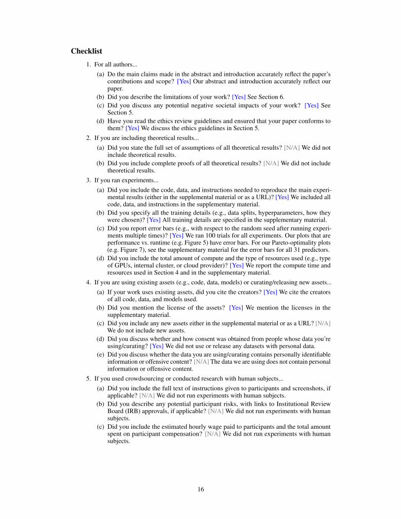
(c) Did you report error bars (e.g., with respect to the random seed after running experi-ments multiple times)? [Yes] We ran 100 trials for all experiments. Our plots that areperformance vs. runtime (e.g. Figure 5) have error bars. For our Pareto-optimality plots(e.g. Figure 7), see the supplementary material for the error bars for all 31 predictors.

(d) Did you include the total amount of compute and the type of resources used (e.g., typeof GPUs, internal cluster, or cloud provider)? [Yes] We report the compute time andresources used in Section 4 and in the supplementary material.

4. If you are using existing assets (e.g., code, data, models) or curating/releasing new assets...(a) If your work uses existing assets, did you cite the creators? [Yes] We cite the creators

of all code, data, and models used.(b) Did you mention the license of the assets? [Yes] We mention the licenses in the

supplementary material.(c) Did you include any new assets either in the supplemental material or as a URL? [N/A]

We do not include new assets.(d) Did you discuss whether and how consent was obtained from people whose data you’re

using/curating? [Yes] We did not use or release any datasets with personal data.(e) Did you discuss whether the data you are using/curating contains personally identifiable

information or offensive content? [N/A] The data we are using does not contain personalinformation or offensive content.

5. If you used crowdsourcing or conducted research with human subjects...(a) Did you include the full text of instructions given to participants and screenshots, if

applicable? [N/A] We did not run experiments with human subjects.(b) Did you describe any potential participant risks, with links to Institutional Review

Board (IRB) approvals, if applicable? [N/A] We did not run experiments with humansubjects.

(c) Did you include the estimated hourly wage paid to participants and the total amountspent on participant compensation? [N/A] We did not run experiments with humansubjects.

16

How Powerful are Performance Predictors in Neural ...

Documents

Transcript of How Powerful are Performance Predictors in Neural ...