arX

iv:0

804.

3474

v1 [

phys

ics.

flu-

dyn]

22

Apr

200

8

Heating of the fuel mixture due to viscous stress ahead of

accelerating flames in deflagration-to-detonation transition

Damir Valiev1,2, Vitaly Bychkov1, V’yacheslav Akkerman1, Lars-Erik Eriksson3

and Mattias Marklund1

1Department of Physics, Umea University, SE–901 87, Umea, Sweden

2Department of Materials Science and Engineering,

Royal Institute of Technology, SE–100 44 Stockholm, Sweden

3Department of Thermo- and Fluid Dynamics,

Chalmers University of Technology, SE–412 96 Goteborg, Sweden

Abstract

The role of viscous stress in heating of the fuel mixture in deflagration-to-detonation transi-

tion in tubes is studied both analytically and numerically. The analytical theory is developed in

the limit of low Mach number; it determines temperature distribution ahead of an accelerating

flame with maximum achieved at the walls. The heating effects of viscous stress and the com-

pression wave become comparable at sufficiently high values of the Mach number. In the case

of relatively large Mach number, viscous heating is investigated by direct numerical simulations.

The simulations were performed on the basis of compressible Navier-Stokes gas-dynamic equa-

tions taking into account chemical kinetics. In agreement with the theory, viscous stress makes

heating and explosion of the fuel mixture preferential at the walls. The explosion develops in an

essentially multi-dimensional way, with fast spontaneous reaction spreading along the walls and

pushing inclined shocks. Eventually, the combination of explosive reaction and shocks evolves into

detonation.

1

I. INTRODUCTION

Deflagration-to-detonation transition (DDT) is one of the most important and least un-

derstood problems in combustion science. It is well known that a deflagration wave propa-

gating from a closed tube end may spontaneously accelerate and trigger an explosion in the

fresh fuel mixture, which goes over to detonation [1, 2, 3, 4, 5, 6]. The mechanism of DDT

was described qualitatively already by Shelkin [2]. According to the Shelkin explanation,

thermal expansion in the burning process produces a strong flow in the unburnt fuel mixture,

which becomes non-uniform because of non-slip at the tube walls. The non-uniform flow

makes the flame curved, which increases the flame surface and hence the volumetric burning

rate; it makes the flow even stronger and leads to flame acceleration. An accelerating flame

pushes compression waves and shocks, the temperature in the fuel mixture increases, the

reaction goes even faster, until explosion happens ahead of the flame front and evolves into

detonation.

For a long time it was a general belief that DDT is impossible without artificial turbu-

lence generation. Since turbulence and turbulent burning are not so well-understood yet,

it presents a major obstacle in developing a theory of flame acceleration and DDT. Only

recently a constructive idea was suggested that DDT may be achieved even in a laminar flow

in tubes with adiabatic walls [7, 8]. Though it is difficult to obtain adiabatic walls in a real

experiment, these conditions may be easily imitated in direct numerical simulations [7, 8].

Starting with this idea, the analytical theory of laminar flame acceleration was developed in

[9, 10]; the theory was quantified by extensive numerical simulations. The idea of laminar

flame acceleration allowed also direct numerical simulations of DDT, e.g. see [7, 11, 12] and

a recent review [6]. The simulations demonstrated many interesting details of the DDT; at

present it is not quite clear, which of them are intrinsic to DDT, making them the backbone

of the process, and which are just supplementary effects of minor importance. One of these

details is heating of the fuel mixture due to viscous stress, which makes the explosion pref-

erential close to the walls. This is different from the classical Shelkin scenario of DDT with

heating produced mainly by the compression/shock waves.

A quantitative analytical theory of explosion triggering by an isentropic compression

wave ahead of an accelerating flame was developed recently in [13]. This theory disregarded

influence of the viscous stress. However, an important role for viscous stress is in line (at

2

least, ideologically) with the model of the DDT, based on hydraulic resistance, see [14] and

references therein. This model had another shortcoming; it was one-dimensional and did

not take into account Shelkin acceleration, which is an intrinsic part of DDT. Thus we came

to the question, how strong the role of viscous stress is in heating of the fuel mixture and

in DDT, taking into account the multi-dimensional Shelkin mechanism of this process. The

purpose of the present paper is to answer this question. The paper considered only the

geometry of smooth tubes, with no obstacles at the walls.

We studied the role of viscous stress both analytically and numerically. The analytical

study is based on the theory of laminar flame acceleration [9]. The theory works excellently

for low Mach numbers, typical for the beginning of flame acceleration, about Ma = 10−3 −10−2. We found temperature profile in the flow ahead of the flame front with maximal

temperature increase achieved at the walls. We show that, at low values of the Mach

number, the role of viscous heating is extremely small, it scales as Ma2. By comparison,

heating due to the compression wave scales as Ma. However, temperature at the walls grows

faster in time than at the axis. According to the theoretical estimates, the heating effects of

viscous stress and of the compression wave become comparable as soon as the Mach number

(defined using total burning rate) reaches values above 0.6. Another interesting point is

that heating due to viscous stress does not depend on the Reynolds number, at least as long

as the Mach number is sufficiently low. When the Mach number becomes about 0.05 and

higher, the theory [9] works only qualitatively, providing order-of-magnitude estimates.

In that range of Mach numbers we investigated the role of viscous heating by direct

numerical simulations. The simulations were performed on the basis of compressible Navier-

Stokes gas-dynamic equations taking into account chemical kinetics. It was again established

that the fuel mixture is heated stronger at the walls than along the tube axis. In agreement

with the analytical theory, we found that heating effects of viscous stress and compression

wave become comparable at large values of the Mach number; viscous heating makes explo-

sion of the fuel mixture preferential at the walls. The explosion develops in an essentially

multi-dimensional way, with fast spontaneous reaction spreading along the walls and push-

ing rather strong shocks inclined with respect to the tube axis. Eventually, the combination

of explosive reaction and shocks evolves into detonation.

The present paper is organized as follows: in Section II we develop the analytical theory

of heating due to viscous stress; in Section III we describe the details of the numerical

3

simulations; in Section IV we present and discuss the results obtained; the paper is concluded

with a short summary.

II. THEORY OF HEATING DUE TO VISCOUS STRESS AHEAD OF ACCELER-

ATING FLAMES

We consider the same geometry as in [9]: a laminar flame propagates in a two-dimensional

(2-D) tube of half-width R with adiabatic walls and non-slip at the walls as shown schemat-

ically in Fig. 1. Burning matter expands as it passes the flame front; density ratio of the

fuel mixture ρf and the burnt gas ρb is typically rather large, Θ = ρf/ρb = 5 − 8. Because

of the thermal expansion, a flame propagating from the closed tube end pushes the unburnt

fuel mixture and generates a flow. It was shown in [9] that the stream ahead of the flame

may be closely approximated by a plane-parallel flow along the walls u = ezuz(x, t).

The normal planar flame velocity Uf provides a natural scaling of velocity dimension for

the problem. However, the total burning rate Uw is different from Uf : it shows how much

fuel mixture is consumed per unit time by the whole flame front and how much energy is

produced. In the standard 2-D model of an infinitely thin flame front, the relative increase

in the burning rate is simply equal to the increase in the total length of the flame front. The

propagating flame generates a flow, which is not uniform because of non-slip at the walls.

Friction retards the gas close to the walls, while flow velocity at the tube axis is larger than

the average one. The non-uniform velocity profile distorts the flame shape, which leads to

increase in Uw and hence to flame acceleration. At sufficiently small values of the Mach

number, neglecting the starting transitional period, the flame has been shown to accelerate

exponentially [9]

Uw/Uf = exp (σUf t/R) . (1)

For 2-D flow, the dimensionless acceleration rate σ was found to be [9]

σ =(Re − 1)2

4Re

(√

1 +4ReΘ

(Re − 1)2− 1

)2

, (2)

where the value Re = UfR/ν plays the role of the Reynolds number for the problem. For

large values of the Reynolds number, Eq. (2) predicts decrease of the acceleration rate

σ = Θ2/Re. (3)

4

In [9], the Navier-Stokes equation was solved as

uz/Uf = (Θ − 1) exp (σUf t/R)cosh µ − cosh(µx/R)

cosh µ − µ−1 sinh µ, (4)

where µ =√

σRe. For large values of the Reynolds number we have µ = Θ, and the flow

resembles qualitatively a combination of two boundary layers at the walls separated by the

main almost uniform stream, see Fig. 2. Paper [9] demonstrated a very good agreement of

the theory with direct numerical simulations of acceleration flames.

Here we find the temperature increase in the fuel mixture ahead of the accelerating flame

using the results above. Similar to [9], we adopt the limit of incompressible flow, which

holds in the case of a sufficiently small Mach number. In that case the equation of thermal

conduction in the fuel mixture is [15]

∂T

∂t+ u · ∇T = χ∇2T +

ν

2CP

(

∂ui

∂xk

+∂uk

∂xi

)2

. (5)

In the case of a shear flow u = ezuz(x, t), with T = T (x, t), Eq. (5) reduces to

∂T

∂t= χ

∂2T

∂x2+

ν

CP

(

∂uz

∂x

)2

. (6)

We introduce standard scalings R, Uf and R/Uf as units of length, velocity and time. In

that case we work with the dimensionless values (η; ξ) = (x; z)/R, τ = Uf t/R, w = uz/Uf ,

and the dimensionless temperature ϑ = T/T0−1. Taking into account the relation for sound

speed in a politropic gas c2

s0 = (γ − 1)CPT0 with heat capacity CP and adiabatic exponent

γ, we rewrite Eq. (6) as

∂ϑ

∂τ=

1

PrRe

∂2ϑ

∂η2+ (γ − 1)

Ma2

0

Re

(

∂w

∂η

)2

. (7)

where Ma0 = Uf/cs0 is the Mach number defined with the help of the planar flame velocity.

The last term in Eq. (7) is specified by the theory [9] with

(

∂w

∂η

)2

= (Θ − 1)2µ2 exp(2στ)sinh2(µη)

(cosh µ − µ−1 sinh µ)2. (8)

We evaluate the possible effect of heating keeping in mind the limit of large Reynolds number

with σ = Θ2/Re, µ = Θ, see Eq. (3). Maximal heating happens close to the wall. Due to

symmetry, we may consider only the wall at η = 1, where sinh(µη) ≈ cosh(µη) ≈ 1

2exp(µη).

5

Such an approximation holds with exponential accuracy exp(−Θ) << 1. In that case we

have close to the wall (at 1 − η << 1)

(

∂w

∂η

)2

=(Θ − 1)2

(µ − 1)2µ4 exp [2στ + 2µ(η − 1)] , (9)

and ∂w/∂η ≈ 0 at the channel axis η = 0. Then Eq. (7) reduces to

∂ϑ

∂τ=

1

PrRe

∂2ϑ

∂η2+ (γ − 1)

Ma2

0(Θ − 1)2

Re(µ − 1)2µ4 exp [2στ + 2µ(η − 1)] . (10)

A particular solution to Eq. (10) may be written as ϑp ∝ exp [2στ + 2µ(η − 1)], which leads

to

ϑp = −(γ − 1) Pr (Θ − 1)2 µ2

2 (2 − Pr) (µ − 1)2Ma2

0exp [2στ + 2µ(η − 1)] . (11)

Here we take into account that µ =√

σRe. A complete solution to Eq. (10) is a superposition

of the particular solution Eq. (11) and the solution to an auxiliary equation

∂ϑ

∂τ=

1

PrRe

∂2ϑ

∂η2, (12)

which also grows in time as ϑ ∝ exp(2στ) so that

2σPrReϑ =∂2ϑ

∂η2. (13)

Solution to the auxiliary Eq. (13) may be found as

ϑa = [A1 exp(kη) + A2 exp(−kη)] exp(2στ), (14)

with unknown amplitudes A1, A2 and

k =√

2σPrRe =√

2Prµ. (15)

The complete solution to Eq. (10) is a superposition of ϑp and ϑa, Eq. (11) and Eq. (14),

satisfying the adiabatic boundary condition at the wall and the symmetry condition at the

channel axis∂ϑ

∂η= 0, η = 0, 1. (16)

Since ϑp is exponentially small at the axis η = 0, we find A1 = A2. Within the same

exponential accuracy, the decaying term A2 exp(−kη) is negligible close to the wall. Thus

we find at the wall η = 1

kA1 exp k = (γ − 1)Pr

(2 − Pr)

(Θ − 1)2 µ3

(µ − 1)2Ma2

0(17)

6

which determines the complete solution close to the wall as

ϑ =(γ − 1)Pr (Θ − 1)2 µ2

2 (2 − Pr) (µ − 1)2Ma2

0exp(2στ)

[

2µ

kexp [k(η − 1)] − exp [2µ(η − 1)]

]

. (18)

The temperature increase at the walls η = 1 is

ϑ =(γ − 1)

2

(Θ − 1)2 µ2

(µ − 1)2

√Pr√

2 +√

PrMa2

0exp(2στ). (19)

Finally, as an evaluation, we consider the limit of large Reynolds number σ = Θ2/Re, µ = Θ,

which leads to the temperature increase

ϑ =(γ − 1)

2Θ2

√Pr√

2 +√

PrMa2

0exp(2στ) =

(γ − 1)

2Θ2

√Pr√

2 +√

PrU2

w/c2

s0. (20)

It is interesting that viscous heating at the wall, Eq. (20), does not depend on the Reynolds

number. Combination Maw = Ma0 exp(στ) = Uw/cs0 determines the running value of the

Mach number for an accelerating flame, which is different from the initial value Ma0 =

Uf/cs0. As an example, we take Θ = 8, Pr = 0.7, γ = 1.4, and find the temperature

increase due to viscous stress ϑ ≈ 4.8Ma2

w = 4.8U2

w/c2

s0.

We compare this result with the heating due to the compression wave found in [13] as

1 + ϑ =

(

1 +γ − 1

2(Θ − 1)Maw

)2

. (21)

Note that the designation ϑ has a different meaning in the present calculations and in [13].

In the case of small Mach numbers we find

ϑ = (γ − 1)(Θ − 1)Maw = (γ − 1)(Θ − 1)Uw

cs0

. (22)

Using the same numbers as before we obtain a temperature increase in a compression wave

ϑ = 2.8Uw/cs0. Thus, for Θ = 8, Pr = 0.7, γ = 1.4, we should expect a comparable

temperature increase due to the compression wave and due to viscous stress at the Mach

number about Maw = Uw/cs0 ≈ 0.6, see Eqs. (20), (22). Besides, heating due to the

compression wave is mostly a 1D process equally strong at the walls and at the channel axis.

As both effects work together, we find preferential heating at the walls. However, we have

to remember that the theory of flame acceleration [9] works quantitatively well only for a

noticeably subsonic flow, Ma = 10−3 − 10−2. At such small Mach numbers heating due to

viscous stress is negligible, since it scales as ϑ ∝ Ma2

w, while heating in a compression wave

7

has another scaling Ma ∝ Maw. At Mach numbers above 0.05 the theory [9] provides only

order-of-magnitude estimates. Direct numerical simulations of the present paper show that,

at Mach numbers above 0.05, flame acceleration goes much slower than in the exponential

regime Eq. (1). The critical value Maw = Uw/cs0 ≈ 0.6 obtained above is also an order-of-

magnitude estimate; it is beyond the rigorous limits of the developed theory. Still, the result

Eq. (20) may be useful even at relatively high values of the Mach number. For comparison,

temperature increase due to viscous stress in the stationary boundary layer produced by a

uniform flow Ua is [16]∆T

Ta

=γ − 1

2

√Pr

U2

a

c2sa

. (23)

Here Ta and csa are the temperature and the sound speed in the uniform flow Ua far away

from the wall. In the present problem flow velocity in the main stream (e.g. at the axis)

plays qualitatively the same role as Ua. Rewriting Eq. (20) in the same form, we find

∆T

Ta

=γ − 1

2

√Pr√

2 +√

Pr

U2

a

c2sa

. (24)

Here we have taken into account that velocity at the axis ahead of an accelerating flame is

related to the total burning rate as Ua = ΘUw, see Eq. (4). The difference between Eqs. (23)

and (24) is then simply in the numerical factor√

2+√

Pr, which is about 2.25 for Pr = 0.7.

An exponentially accelerating flame produces about half the temperature increase at the

wall compared to that from the stationary boundary layer. Thus one would expect that the

temperature increase at Maw = 0.05 and above is somewhere between predictions of Eqs.

(23) and (24). In order to investigate the role of viscous heating at relatively large values

of the Mach number we performed direct numerical simulations. We stress once more that

both formulas (23), (24) predict viscous heating independent of the Reynolds number. This

conclusion is of great help in numerical simulations, since it allows investigating the process

even for rather low values of the tube width.

III. BASIC EQUATIONS OF THE DIRECT NUMERICAL SIMULATIONS

We performed direct numerical simulations of the 2-D hydrodynamic and combustion

equations including transport processes (thermal conduction, diffusion, viscosity) and chem-

ical kinetics with an Arrhenius reaction. The equations read

∂ρ

∂t+

∂

∂xi

(ρui) = 0, (25)

8

∂

∂t(ρui) +

∂

∂xj

(ρuiuj + δijp − γij) = 0, (26)

∂

∂t

(

ρε +1

2ρuiui

)

+∂

∂xj

(

ρujh +1

2ρuiuiuj + qj − uiγij

)

= 0, (27)

∂

∂t(ρY ) +

∂

∂xi

(

ρuiY − µ

Sc

∂Y

∂xi

)

= −ρY

τR

exp (−E/RpT ) , (28)

where Y is the mass fraction of the fuel mixture, ε = QY + CV T is the internal energy,

h = QY + CpT is the enthalpy, Q is the energy release in the reaction, CV , Cp are the heat

capacities at constant volume and pressure. It was assumed that the heat capacities do not

depend on the chemical reaction. The stress tensor γij and the energy diffusion vector qj

take the form

γij = µ

(

∂ui

∂xj

+∂uj

∂xi

− 2

3

∂uk

∂xk

δij

)

, (29)

qj = −µ

(

Cp

Pr

∂T

∂xj

+Q

Sc

∂Y

∂xj

)

, (30)

where µ ≡ ρν is the dynamic viscosity, Pr and Sc are the Prandtl and Schmidt numbers,

respectively. To avoid the Zeldovich (thermal-diffusion) instability we take the unit Lewis

number Le ≡ Pr/Sc = 1, with Pr = Sc = 0.75. The dynamical viscosity is µ = 1.7 ×10−5Ns/m2. The fuel-air mixture and burnt matter are assumed to be a perfect gas with

a constant molar mass m = 2.9 × 10−2kg/mol, with CV = 5Rp/2m, Cp = 7Rp/2m, where

Rp ≈ 8.31J/(mol ·K) is the perfect gas constant. The adiabatic index is γ ≡ CP /CV = 1.4.

The equation of state is

P = ρRpT/m. (31)

We used the initial temperature of the fuel mixture Tf = 300K, initial pressure Pf = 105Pa,

and initial expansion ratio Θ0 = 8. The initial Mach number is Ma0 = Uf/cs0 = 0.04. Eq.

(28) describes a single irreversible reaction of the first order, where the reaction rate obeys

the Arrhenius law with the activation energy Ea and the factor of time dimension τR. In the

simulations, the value of Uf is determined by the choice of thermal-chemical parameters such

as Ea, τR, and the energy release in the reaction Q = (Θ0 − 1)CPTf . In order to have better

resolution of the reaction zone, we took Ea/RpTf = 32 in the simulations. Note that the

9

process of viscous heating addressed in our paper does not depend on the activation energy.

The factor τR was adjusted to obtain a particular value of the planar flame velocity Uf by

solving the associated eigen-value problem. The flame thickness is conventionally defined as

Lf ≡ µ

PrρfUf

, (32)

where ρf = 1.16kg/m3 is the initial mixture density. However, we would like to stress that

the value (32) is just a thermal-chemical parameter of length dimension in the problem; the

characteristic size of the burning zone may be an order of magnitude larger [17].

In the studies of flame acceleration [9, 10], the main parameter of simulations was the tube

width 2R, which controlled the Reynolds number. In the present paper we are interested

in thermal heating due to viscous stress. According to the present theory and the classical

results [16], viscous heating does not depend on the Reynolds number (or this dependence is

extremely weak). For this reason, to study the effect, it is sufficient to perform simulations

only for one channel width. The channel width was set to 2R = 40Lf , which implied the

Reynolds number related to the planar flame velocity Re = UfR/ν = R/LfPr = 26.7. The

Reynolds number related to the flow Re = 〈uz〉 2R/ν may be larger by several orders of

magnitude due to flame acceleration and thermal expansion of the burning gas. We took

non-slip and adiabatic boundary conditions at the channel walls:

u = 0, n · ∇T = 0. (33)

where n is a normal vector at the wall. At the open channel end non-reflecting boundary

conditions are used; the boundary conditions were tested in [17]. We used two types of

initial conditions: 1) a hemispherical flame ”ignited” at the channel axis at the closed end

of the channel, or 2) a planar flame front.

The internal structure of the flame imitated the analytical solution by Zel’dovich and

Frank-Kamenetskii [3]. Particularly, for the hemispherical case it was given by

T = Tf + Tf(Θ − 1) exp(

−√

x2 + z2/Lf

)

, if z2 + x2 > r2

f . (34)

T = ΘTf , if z2 + x2 < r2

f . (35)

Y =Θ − T/Tf

Θ − 1, P = Pf , u = 0. (36)

10

Here rf is the radius of initial flame ball at the closed end of the channel. For an initially

planar flame shape Eq. (34) is replaced by

T = Tf + Tf(Θ − 1) exp [− (z − z0) /Lf ] , (37)

if z > z0, with Eq. (35) for z < z0 (z0 denotes the initial flame position).

We simulated flame dynamics and DDT using a 2-D Cartesian Navier-Stokes solver with

chemical reactions developed at Volvo Aero. The code is based on the cell-centered finite-

volume scheme developed by L.-E. Eriksson [18, 19]. The numerical method has proved to

be robust for modelling different kinds of complex reacting flows. The TVD-limiting is used

where applicable to prevent overshoots in flow field properties in regions of high gradients.

The code has been validated by solving various hydrodynamic problems [18, 19, 20], and

was utilized successfully in simulations of laminar flames at different conditions of burning

[9, 10, 12, 17, 21, 22, 23, 24, 25, 26].

The grids used in present simulations were non-uniform with higher resolution around

the flame front and pressure waves and lower resolution in other parts of the calculation

domain. Grid resolution varied gradually from one zone to another along the tube. Using

this method we avoided processing a too large number of cells. Square cells of the size 0.2Lf

were used in the flame domain to ensure isotropic propagation of the curved flame in x and

y directions. In [17] we demonstrated that such a grid is sufficient to resolve even a strongly

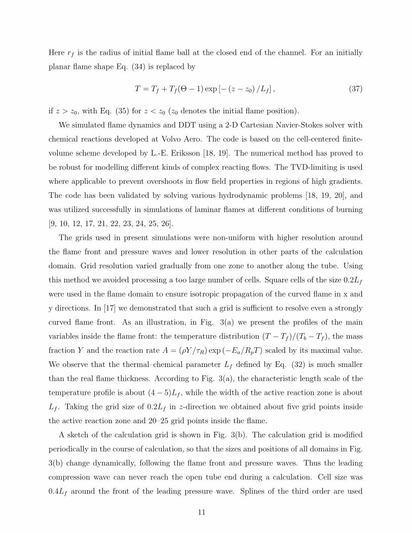
curved flame front. As an illustration, in Fig. 3(a) we present the profiles of the main

variables inside the flame front: the temperature distribution (T − Tf )/(Tb − Tf ), the mass

fraction Y and the reaction rate A = (ρY /τR) exp (−Ea/RpT ) scaled by its maximal value.

We observe that the thermal–chemical parameter Lf defined by Eq. (32) is much smaller

than the real flame thickness. According to Fig. 3(a), the characteristic length scale of the

temperature profile is about (4− 5)Lf , while the width of the active reaction zone is about

Lf . Taking the grid size of 0.2Lf in z-direction we obtained about five grid points inside

the active reaction zone and 20–25 grid points inside the flame.

A sketch of the calculation grid is shown in Fig. 3(b). The calculation grid is modified

periodically in the course of calculation, so that the sizes and positions of all domains in Fig.

3(b) change dynamically, following the flame front and pressure waves. Thus the leading

compression wave can never reach the open tube end during a calculation. Cell size was

0.4Lf around the front of the leading pressure wave. Splines of the third order are used

11

for re-interpolation of the flow variables during periodic grid reconstruction to preserve the

second order accuracy of the numerical scheme. We performed several test simulation runs

with different resolution between 0.1 and 0.2Lf in the flame domain. The tests demonstrated

that the difference in the flame velocity, pre-detonation time and distance does not exceed

10% for different resolutions.

IV. SIMULATION RESULTS

We performed direct numerical simulation of flame dynamics and detonation triggering

in a tube of width 2R = 40Lf with non-slip walls. The flame propagated from the closed

tube end to the open one; a semi-infinite tube was imitated by using non-reflecting boundary

conditions at the open end and by adjusting the mesh to the leading pressure wave. We

started the simulations either with a hemispherical flame ignited at the tube axis or with a

planar flame front. Fig. 4 shows velocity of the combustion front in the laboratory reference

frame of the tube, Ulab/Uf , in the case of hemispherical ignition; the velocity was calculated

as the average over the reaction front. Flame dynamics involves several velocity parameters,

which have quite different physical meaning and may differ quantitatively by one or two

orders of magnitude. First, we have a planar flame velocity Uf , which characterizes local

normal velocity of the flame front relative to the moving fuel mixture (at least in the model

of an infinitely thin front). The value Uf works as a standard velocity scaling in the problems

of flame dynamics. To be accurate, Uf depends on thermal and chemical parameters of the

fuel mixture, which vary in the process of detonation triggering. Here Uf designates the

initial planar flame velocity. Second, we have the burning rate Uw, which specifies total

amount of fuel mixture burnt per unit time (see also Section II). The burning rate Uw may

exceed Uf by several orders of magnitude in the process of flame acceleration. Still, the

value Uw does not describe flame propagation in any particular reference frame except for

the case of stationary or statistically-stationary curved flames like in [22, 23, 26, 27, 28].

Flame propagating from the closed end pushes a strong flow in the fuel mixture. In the

incompressible case, average velocity of the flow is 〈uz〉 = (Θ − 1)Uw, where averaging is

performed over the channel cross-section. The flow drifts the flame, and the drift velocity

is different for different parts of the flame front. For this reason, the burning rate Uw is

also different from flame velocity in the laboratory reference frame, with respect to the tube

12

walls, Ulab. We stress that Fig. 4 presents flame velocity in the laboratory reference frame,

Ulab, not the burning rate Uw. In the case of an essentially subsonic flame, we have a simple

relation Ulab = ΘUw, which may also provide an estimate in the case of finite Mach numbers.

Different velocity parameters imply different Mach numbers as well, which we designate by

Ma0 = Uf/cs0, Maw = Uw/csa, Malab = Ulab/csa; label ”a” refers to the position at the

channel axis just ahead of the flame front. Taking a rather low initial Mach number related

to the planar flame velocity Ma0 = 0.04 with Θ = 8, we have immediately Malab = 0.32,

which is not so low. Soon after ignition, in a short time about (0.2 − 0.3)R/Uf , burning

rate increases by order of magnitude in the process of precursor acceleration [29, 30]. As a

result, quite quickly the Mach number Malab becomes comparable to unity. We also point

out that Maw, Malab take into account variations of the sound speed in the fuel mixture in

time and space; scaled sound speed csa/Uf is shown by the dashed line in Fig. 4(a).

Transition from one combustion regime to another (flame-explosion-detonation) may be

clearly seen by drastic changes in the front velocity. In the flame regime, we can see front

acceleration, which involves two different physical mechanisms. First, we observe a short

period of precursor acceleration, related to the hemispherical geometry of flame ignition.

This type of acceleration is possible even in the case of friction-free walls. Precursor ac-

celeration goes noticeably faster than the Shelkin mechanism, but this process is limited in

time. Precursor acceleration for a cylindrical tube was investigated experimentally in [29]

and numerically in [30]. The paper [30] presented also the analytical theory of the process.

In the present geometry of a 2-D channel the precursor acceleration is somewhat different

from the cylindrical case; still, the basic features of the process remain the same.

The precursor acceleration is followed by acceleration due to the Shelkin mechanism

produced by thermal expansion and non-slip at the walls. The theory of the Shelkin ac-

celeration in incompressible flows has been developed in [9, 10]. However, in the present

case Mach number Malab is comparable to unity or above, and the incompressible theory

of flame acceleration describes the process only qualitatively. A dashed line in Fig. 4(a)

shows the exponential growth predicted by the incompressible theory Eq. (1); it goes well

above the numerical results as soon as the precursor acceleration is over. Investigation of

the compressibility effects on flame acceleration is beyond the scope of the present paper;

this is work for the future. Still, as a preliminary result, Fig. 4(b) shows the flame veloc-

ity in log-log variables. In order to elucidate the transition effects related to a particular

13

geometry of flame ignition, we have performed two simulation runs: that of a flame ignited

at the tube axis and one for a flame ignited as a planar front. In the first case we have

precursor acceleration of the flame front, while in the second case this effect is missing. As

we can see, both simulation runs tend to the same asymptotic regime of flame acceleration

with Ulab ∝ (Uf t/R)n, where n ≈ 0.36. More detailed investigation of the process will be

presented elsewhere. It is well known that flame is subsonic; still, this rule applies to the

burning rate Uw, not to Ulab. In Fig. 4(b), Ulab crosses the sonic line at the time instant

about Uf t/R = 30. This time instant is often called run-up time to supersonic flames [31].

An accelerating flame produces a flow in the fuel mixture, which is non-uniform because

of the non-slip boundary conditions. A characteristic velocity profile is shown in Fig. 5:

the results of numerical simulations are compared to the predictions of the incompressible

theory [9]. The velocity profile is calculated at different time instants just ahead of the flame

front and scaled by the maximum velocity value at the tube axis. Both the theory and the

present simulations demonstrate the same qualitative structure of the flow, which consists

of an almost uniform stream close to the axis and transitional (boundary) layers close to

the walls. The velocity profile is in a good agreement with the incompressible case, not

only qualitative, but even quantitative. A non-uniform viscous flow implies stress, which is

stronger close to the channel walls. As a consequence, one should expect additional heating

of the fuel mixture due to the viscous stress, as discussed in Section II. In this Section, our

main goal is to investigate the process of viscous heating numerically and to compare it to

the theory of Section II.

The temperature increase in the fuel mixture just ahead of the flame front is shown in Fig.

6 as a function of time and at two positions: at the tube axis and at the channel wall. We

can see that, within a short time after ignition Uf t/R = 0.2− 0.3, the temperature increase

is already different from zero, being about ∆T/T0 ≈ 0.25. This happens because of the

leading shock wave, pushed by the flame in the process of precursor acceleration. The flow

velocity behind the shock is about ∆uz/Uf ≈ Θ−1, and thermal expansion is typically quite

strong. Therefore, in spite of a small initial Mach number Ma0 = 0.04, the flow velocity is

not so small in comparison with sound speed even for a planar flame front, ∆uz/cs0 = 0.28.

Precursor acceleration makes this value even larger. At the beginning, temperature increase

at the walls and at the tube axis is practically the same, which illustrates almost 1D structure

of the compression wave. As time goes on, the flame accelerates, the Mach number of the

14

flow increases and heating due to viscous stress becomes noticeable in agreement with the

theory of Section II. By the time of explosion, Uf t/R ≈ 4.38, difference between temperature

at the axis and at the walls is noticeable; still, this difference is not as strong as predicted

by the theory. In order to compare the numerical simulations and the theory quantitatively,

in Fig. 7 we plot temperature increase versus Mach number Malab. In that case we separate

heating in the compression wave (at the axis), and the effect of viscous stress as temperature

difference between the wall and the axis, Twall − Taxis. Heating in the compression wave at

the axis is shown by squares. Temperature at the axis increases almost linearly with the

Mach number, in agreement with the theory, Eq. (21), presented by the solid line. The

theoretical prediction holds for a 1D isentropic flow; small deviations of the theory and

simulations indicate that the flow is not completely 1D and isentropic. Two other solid

lines show theoretical predictions for temperature increase due to viscous stress ahead of an

exponentially accelerating flame, Eq. (24), and in a stationary boundary layer, Eq. (23).

These two formulas present two limiting cases of strong acceleration and no acceleration at

all. As we pointed out, at relatively high values of the Mach number, the flame acceleration

is much slower than exponential. By this reason it is natural to expect that the numerical

points should be somewhere in between the predictions of Eqs. (23) and (24). Indeed, Fig. 7

shows that this is the case; the numerical results come rather close to that of Eq. (24), being

a little above the theoretical curve. Only at the end of the simulation run, temperature at the

wall increases drastically, which indicates the beginning of the explosion. It is also interesting

to look at the temperature distribution in the channel. Fig. 8 compares temperature profiles

at different distances ahead of the flame front at the time instant Uf t/R = 3.43 to the

theoretical result Eq. (18). The theoretical predictions look quite similar to the numerical

results: all the time we observe the effect of viscous heating well-localized at the walls. Still,

the theory predicts a self-similar temperature profile independent of position, since it was

developed for an exponentially accelerating flame in an incompressible flow. In the numerical

simulations flame acceleration is not exponential, the flow is not incompressible, and the

temperature profile changes in space and time. As we can see in Fig. 8, the transitional zone

of viscous heating is wider close to the flame front, and it becomes more localized far away

from the flame.

As we can see, heating due to viscous stress is not large in comparison with that in a

compression wave, and, in principle, explosion theoretically could be possible even without

15

viscous heating. Fig. 9 presents temperature field snapshots in the area of the accelerating

flame from beginning of the explosion till detonation. Prior to the explosion, we can see light

blue strips along the walls indicating regions of viscous heating. Still, Arrhenius reactions are

extremely sensitive to temperature; even this slight non-uniformity influences strongly the

structure of the explosion. The explosion may be observed already at the second snapshot:

it develops in the form of two narrow tongues spreading fast along the tube walls from the

flame front to the fuel mixture. Temperature in the explosion zone is noticeably higher

than it was behind the flame front. The tongues grow in length and width, until the original

flame front becomes engulfed in the explosion. However, even at that time the explosion front

remains essentially multi-dimensional: a large amount of the unburned matter separates two

explosion tongues. The explosion pushes inclined pressure waves, well seen in Fig. 9 by the

light blue color. Intersection of the pressure waves increases temperature at the channel axis,

reduces the reaction time, until a bridge is formed between two tongues of the explosion.

As two tongues meet, they soon develop into detonation, which can be seen in the last two

snapshots of Fig. 9. Meeting of two explosion tongues may be also seen in Fig. 4. as an

extremely sharp peak in the velocity dependence. Strictly speaking, this peak is infinitely

sharp and high, since it corresponds to a singularity of pocket formation. In Fig. 4, we cut

down the peak to make the plot more illustrative. In the present calculations, DDT distance

is 330R, but this value is, of course, sensitive to a particular chemical kinetics.

V. SUMMARY

The purpose of the present paper was to investigate the role of viscous heating in DDT.

We solved this problem both analytically and by direct numerical simulations. The ana-

lytical theory was developed within the approximation of incompressible flow, which holds

at sufficiently low values of the Mach number. On the contrary, the numerical simulations

were performed for relatively large Mach numbers. Both theory and numerical simulations

demonstrated that the role of viscous heating increases with the Mach number. Viscous

stress makes temperature higher at the channel walls in comparison with the axis. Temper-

ature profile in the channel is given by Eq. (18), temperature increase at the wall due to

viscous stress is determined by Eq. (24). The theoretical results agree rather well with the

numerical simulations, though, when making a comparison, one has to take into account

16

much slower flame acceleration at larger values of the Mach number. Even just before the

explosion, additional temperature increase due to viscous heating is noticeably smaller than

the temperature increase in the compression wave. Thus, viscous heating should be treated

only as a supplementary process in DDT. In principle, DDT could be possible with heating

provided by the compression wave only in line with the Shelkin scenario [2, 5, 13]. Still,

neglecting viscous heating in a theoretical model like [13] may lead to considerable disagree-

ment in the time and distance of detonation triggering predicted by the theory and obtained

in experiments/numerical simulations. Viscous heating makes explosion triggering easier

and faster because of extreme sensitivity of Arrhenius reactions to temperature variations.

In a certain sense, it plays the same role as hot spots: it is not necessary, but helpful. Non-

uniform temperature distribution leads to an essentially multi-dimensional structure of the

explosion, which pushes inclined pressure waves and eventually develops into detonation.

VI. ACKNOWLEDGEMENTS

This work was supported by the Swedish Research Council (VR). Numerical simulations

were performed at High Performance Computer Center North (HPC2N), Umea, Sweden,

within SNAC project 007-07-25. The authors also wish to thank Arkady Petchenko and

Michael Modestov for useful discussions.

17

[1] F. A. Williams, Combustion Theory, Benjamin, Redwood City, CA, 1985.

[2] K. I. Shelkin, Zh. Exp. Teor. Fiz. 10, 823 (1940).

[3] Ya. B. Zeldovich, G. I. Barenblatt, V. B. Librovich, G. M. Makhviladze, Mathematical Theory

of Combustion and Explosion, Consultants Bureau, New York, 1985.

[4] J. E. Shepherd, J. H. S. Lee, in Major Research Topics in Combustion, p. 439, Springer Verlag,

Hampton, VA, 1992.

[5] G. Roy, S. Frolov, A. Borisov, D. Netzer, Prog. En. Combust. Sci. 30, 545 (2004).

[6] E. Oran, V. Gamezo, Combust. Flame 148 4 (2007).

[7] L. Kagan, G. Sivashinsky, Combust. Flame 134, 389 (2003).

[8] J. D. Ott, E. S. Oran, J. D. Anderson, AIAA Journal 41, 1391 (2003).

[9] V. Bychkov, A. Petchenko, V. Akkerman, L.-E. Eriksson, Phys. Rev. E 72, 046307 (2005).

[10] V. Akkerman, V. Bychkov, A. Petchenko, L.-E. Eriksson, Combust. Flame 145, 206 (2006).

[11] L. Kagan, D. Valiev, M. Liberman, G. Sivashinsky, in Proceedings of Pulsed and Continuous

Detonations, eds. G. Roy, S. Frolov, J. Sinibaldy, Torus Press Ltd, p. 119 (2006).

[12] M. Liberman, G. Sivashinsky, D. Valiev, L.-E. Eriksson, J. Trans. Phenomena 8, 253 (2006).

[13] V. Bychkov, V. Akkerman, Phys. Rev. E 73, 066305 (2006).

[14] I. Brailovsky, G. Sivashinsky, Combust. Flame 122, 492 (2000).

[15] L. D. Landau, E. M. Lifshitz, Fluid Mechanics (Pergamon Press, Oxford, 1989).

[16] H. Schlichting, Theory of a Boundary Layer, Verlag G. Braun, Karlsruhe, 1969.

[17] V. Akkerman, V. Bychkov, A. Petchenko, L.-E. Eriksson, Combust. Flame 145, 675 (2006).

[18] L.-E. Eriksson, A third-order accurate upwind-based finite volume scheme for unsteady com-

pressible viscous flows, VAC Report 9370-154, Volvo Aero Corporation (1993).

[19] L.-E. Eriksson, Development and validation of highly modular solver versions G2DFlow and

G3DFlow series for compressible viscous reactive flow, VAC Report 9970-1162, Volvo Aero

Corporation (1995).

[20] L.-E. Eriksson, Comp. Meth. Mech. Eng. 64, 95 (1987).

[21] V. Bychkov, M. Liberman, Phys. Rep. 325, 115 (2000).

[22] V. Bychkov, S. Golberg, M. Liberman, L.-E. Eriksson, Phys. Rev. E 54, 3713 (1996).

[23] O. Travnikov, V. Bychkov, M. Liberman, Phys. Rev. E 61, 468 (2000).

18

[24] A. Petchenko, V. Bychkov, V. Akkerman, L.-E. Eriksson, Phys. Rev. Lett. 97, 164501 (2006).

[25] A. Petchenko, V. Bychkov, V. Akkerman, L.-E. Eriksson, Combust. Flame 149, 418 (2007).

[26] M. Liberman, M. Ivanov, O. Peil, D. Valiev, and L.-E. Eriksson, Combust. Theory Model. 7,

653 (2003).

[27] S. Kadowaki, T. Hasegawa, Prog. Energy Combust. Sci. 31, 193 (2005).

[28] A. Petchenko, V. Bychkov, L.-E. Eriksson, and A. Oparin, Combust. Theory Model. 10, 581

(2006).

[29] C. Clanet, G. Searby, Combust. Flame 105, 225 (1996).

[30] V. Bychkov, V. Akkerman, G. Fru, A. Petchenko, L. E. Eriksson, Combust. Flame 150, 263

(2007).

[31] M. Kuznetsov, V. Alekseev, I. Matsukov, S. Dorofeev, Shock Waves 14, 205 (2005).

19

FIG. 1: Flame propagating in a tube with non-slip walls.

FIG. 2: The velocity profile uz scaled by the amplitude Umax. The solid line shows the theoretical

result Eq. (4). The markers correspond to the simulation results of [9] for Re = 50, Pr = 0.5

at the distances 10R; 20R; 35R (circles, triangles and crosses) from the flame at the time instance

Uf t/R = 1.15. The arrows illustrate the direction of the flow.

20

(a)

(b)

FIG. 3: Illustration of the grid. (a) Profiles of the scaled temperature (T −Tf )/(Tb −Tf ), the mass

fraction Y and the reaction rate A = (ρY/τR) exp (−Ea/RpT ) scaled by its maximal value within

the flame front. (b) The adaptive grid used in numerical simulations.

21

(a)

(b)

FIG. 4: (a) Scaled velocity of the reaction front (flame-explosion-detonation) in the laboratory

reference frame, Ulab/Uf . One dashed line presents theoretical predictions for the incompressible

flow. The other dashed line shows scaled sound speed, csa/Uf . (b) The same plot in log-log

variables for a flame ignited at the channel axis (with precursor acceleration) and as a planar front

(no precursor acceleration).

22

FIG. 5: The velocity profile uz scaled by the amplitude Umax. The solid line shows the theoretical

result Eq. (4). The markers correspond to the present simulation results just ahead of the flame

front at the time instants Uf t/R = 0.92; 1.74; 3.43.

23

FIG. 6: Temperature increase at the wall and at the channel axis versus time.

24

FIG. 7: Temperature increase versus Mach number in the laboratory reference frame. Solid lines

show theoretical predictions for temperature increase in the compression wave at the axis, Eq.

(21), and additional increase due to viscous stress at the wall, Eqs. (23), (24). The dashed lines

and the markers show respective numerical results.

25

FIG. 8: Scaled temperature profile (T − Taxis)/(Twall − Taxis). The solid line shows the theoret-

ical result Eq. (18). The markers correspond to the present simulation results at the distances

(6; 425; 930)Lf ahead of the flame front at the time instant Uf t/R = 3.43.

26

FIG. 9: Temperature field during DDT for the time period from Uf t/R = 4.38 to Uf t/R = 4.58

with equal time intervals between the snapshots.

27