On the dynamics of multi-dimensional detonation
51
J. Fluid Mech. (1996), uol. 309, pp. 225-215 Copyright 0 1996 Cambridge University Press 225 On the dynamics of multi-dimensional detonation By JIN YAO AND D. SCOTT STEWART? Department of Theoretical and Applied Mechanics, University of Illinois, Urbana, IL 61801, USA (Received 25 January 1995 and in revised form 22 September 1995) We present an asymptotic theory for the dynamics of detonation when the radius of curvature of the detonation shock is large compared to the one-dimensional, steady, Chapman-Jouguet (CJ) detonation reaction-zone thickness. The analysis considers additional time-dependence in the slowly varying reaction zone to that considered in previous works. The detonation is assumed to have a sonic point in the reaction- zone structure behind the shock, and is referred to as an eigenvalue detonation. A new, iterative method is used to calculate the eigenvalue relation, which ultimately is expressed as an intrinsic, partial differential equation (PDE) for the motion of the shock surface. Two cases are considered for an ideal equation of state. The first corresponds to a model of a condensed-phase explosive, with modest reaction rate sensitivity, and the intrinsic shock surface PDE is a relation between the normal detonation shock velocity, D,, the first normal time derivative of the normal shock velocity, D,,, and the shock curvature, IC. The second case corresponds to a gaseous explosive mixture, with the large reaction rate sensitivity of Arrhenius kinetics, and the intrinsic shock surface PDE is a relation between the normal detonation shock velocity, D,, its first and second normal time derivatives of the normal shock velocity, b,, B,, and the shock curvature, IC, and its first normal time derivative of the curvature, k. For the second case, one obtains a one-dimensional theory of pulsations of plane CJ detonation and a theory that predicts the evolution of self-sustained cellular detonation. Versions of the theory include the limits of near-CJ detonation, and when the normal detonation velocity is significantly below its CJ value. The curvature of the detonation can also be of either sign, corresponding to both diverging and converging geometries. 1. Introduction Previous work, Stewart & Bdzil (1988), Bdzil & Stewart (1989), has developed an asymptotic theory for weakly curved, slowly varying detonation that propagates near the Chapman-Jouguet (CJ) velocity, DcJ, for the explosive, and has found that the normal detonation shock velocity D, is a function of the total shock curvature, IC. We call this relation, the (D,,K)-relation, and it is a partial differential equation (PDE) for the motion of the detonation shock surface. The functional form of the (D,, Ic)-relation follows from an asymptotic argument and is solely determined by the explosive material's equation of state and reaction rate law. In this paper, we extend the asymptotic analysis by considering the additional time- dependence which is required when the normal detonation shock velocity deviates t Author to whom correspondence should be addressed.
-
Upload
independent -
Category
Documents
-
view
2 -
download
0
Transcript of On the dynamics of multi-dimensional detonation
J. Fluid Mech. (1996), uol. 309, p p . 225-215 Copyright 0 1996 Cambridge University Press
225
On the dynamics of multi-dimensional detonation
By JIN YAO AND D. SCOTT STEWART? Department of Theoretical and Applied Mechanics, University of Illinois, Urbana, IL 61801, USA
(Received 25 January 1995 and in revised form 22 September 1995)
We present an asymptotic theory for the dynamics of detonation when the radius of curvature of the detonation shock is large compared to the one-dimensional, steady, Chapman-Jouguet (CJ) detonation reaction-zone thickness. The analysis considers additional time-dependence in the slowly varying reaction zone to that considered in previous works. The detonation is assumed to have a sonic point in the reaction- zone structure behind the shock, and is referred to as an eigenvalue detonation. A new, iterative method is used to calculate the eigenvalue relation, which ultimately is expressed as an intrinsic, partial differential equation (PDE) for the motion of the shock surface. Two cases are considered for an ideal equation of state. The first corresponds to a model of a condensed-phase explosive, with modest reaction rate sensitivity, and the intrinsic shock surface PDE is a relation between the normal detonation shock velocity, D,, the first normal time derivative of the normal shock velocity, D,,, and the shock curvature, IC. The second case corresponds to a gaseous explosive mixture, with the large reaction rate sensitivity of Arrhenius kinetics, and the intrinsic shock surface PDE is a relation between the normal detonation shock velocity, D,, its first and second normal time derivatives of the normal shock velocity, b,, B,, and the shock curvature, IC, and its first normal time derivative of the curvature, k. For the second case, one obtains a one-dimensional theory of pulsations of plane CJ detonation and a theory that predicts the evolution of self-sustained cellular detonation. Versions of the theory include the limits of near-CJ detonation, and when the normal detonation velocity is significantly below its CJ value. The curvature of the detonation can also be of either sign, corresponding to both diverging and converging geometries.
1. Introduction Previous work, Stewart & Bdzil (1988), Bdzil & Stewart (1989), has developed an
asymptotic theory for weakly curved, slowly varying detonation that propagates near the Chapman-Jouguet (CJ) velocity, DcJ, for the explosive, and has found that the normal detonation shock velocity D, is a function of the total shock curvature, IC.
We call this relation, the (D,,K)-relation, and it is a partial differential equation (PDE) for the motion of the detonation shock surface. The functional form of the (D,, Ic)-relation follows from an asymptotic argument and is solely determined by the explosive material's equation of state and reaction rate law.
In this paper, we extend the asymptotic analysis by considering the additional time- dependence which is required when the normal detonation shock velocity deviates
t Author to whom correspondence should be addressed.

226 J . Yao and D. S . Stewart
significantly from its CJ value, or when the additional dynamics of low-frequency, acoustics are considered for explosives with a sensitive reaction rate. The new descriptions can include both accelerating and decelerating detonations, and the curvature of the detonation can be positive or negative for diverging (convex) or converging (concave) geometries. The only restriction is that the detonation structure has an essentially sonic character. This analysis is a significant extension and replaces the older theory, referred to above, where the detonation normal shock speed is, by assumption, always restricted to be near-CJ. In particular, this new theory re- introduces the time derivatives which are absent in the older theory. However, an assumption of slow variation in time, measured on the scale of the particle transit time through the reaction zone, is still required to carry out a rational set of approximations, where the one-dimensional steady structure holds to leading order.
The asymptotic technique for analysing the quasi-steady equations in intrinsic coor- dinates, used in Stewart & Bdzil (1988) and elaborated on in Klein & Stewart (1993), involves an expansion technique in the (U:, ,?.)-plane, where U , is the normal velocity in a shock-attached frame and ,?. is a progress variable for a forward exothermic reaction. In the simplest version of the theory, there are essentially two layers, a main reaction layer (MRL), which is a layer that connects the desired (U,, A) integral curve to the shock boundary conditions at A = 0, and a transonic layer (TSL), that connects to the singular point at the intersection of the sonic and thermicity locus, near the end of the reaction layer, with A near 1. Matching the expansions from either side gives the D,, K eigenvalue relation, albeit in a somewhat tedious fashion. (When the dimensionless activation energy is large, then the MRL has a induction-zone (IZ) layer near the shock, and it is appropriate to consider a distinguished limit that reflects how the shape changes of the shock can affect the post-shock temperature. This analysis was recently considered for the steady case, Yao & Stewart (1995).)
The quasi-steady eigenvalue problem, posed in 94, can be solved numerically, for finite IC, by an iterative shooting technique that starts from the shock and integrates towards the sonic point or vice versa. Numerically, this procedure is found to be quite robust. For asymptotically small curvature, the numerical shooting technique is equivalent to a method of successive approximation (MSA) technique, which is an alternative to the layer expansion technique. The MSA technique formally integrates a nearly conservative form of the equations in the normal coordinate, from the shock to the generalized CJ-point to obtain integral equations. Integral equations are then used to generate non-singular asymptotic expansions, where the first approximation is a one-dimensional steady, or quasi-steady state. The procedure is general and might be useful for substantial extensions of the related theory : specifically, complex chemistry. It would seem that in most cases that we have tried so far, only one or two iterations are really all that are required to obtain the essential asymptotic results. Like the numerical approach, the technique is likely to be robust. In what follows, we present the derivation of an unsteady detonation structure that includes acceleration effects using the MSA technique; however we have also carried out the same calculations in 95, using the layer expansion procedure, and those details can be found in Yao (1996).
In $2 we cite the governing equations, explain the intrinsic, shock-attached coordi- nates used, and present the reduced equations that are analysed subsequently. Section 2 is read with the help of Appendices A and B, which give details on Betrand-intrinsic coordinates and the reduced governing equations, respectively. Section 3 briefly re- views the one-dimensional steady and quasi-steady states. Section 4 derives the result for quasi-steady, near-CJ detonation and in particular uses the MSA technique in an

Dynamics of multi-dimensional detonation 227
integral formulation and succinctly derives all the results of the older theory. Section 5 derives the asymptotic results for slowly varying, unsteady, weakly curved detonation and a (b,, D,, #)-relation that governs the shock dynamics, which is appropriate for a model of condensed explosive with low or zero activation energy. The strong-shock approximation is employed. Here bn is the first normal time derivative of D,. Section 6 separately considers the special case of large activation energy and derives a richer surface evolution equation, which is a relation between &, b,, D,, K and k. Further analysis of this equation in the limit of zero curvature leads to a description of pulsat- ing detonation for the plane, CJ detonation, governed by a second-order ODE, with a correspondingly simple stability theory. The same equation with curvature admits solutions that correspond to detonations that have self-sustained cellular instability, generated by transverse waves on the shock.
2. Governing equations A standard model of explosive materials is adopted: a compressible Euler fluid, with
exothermic reaction. The basic mechanical variables are the velocity, u, the density p and the thermodynamic pressure p . The specific volume is o = l / p . Chemistry is modelled in the equation of state by introducing an exothermic chemical reaction, represented by the progress variable, A. Specification of an equation of state (EOS) of the form e(p, p, A), and a rate law, r ( p , p, A) for A, is assumed to describe the explosive.
We will further assume the explosive has a polytropic equation of state and an Arrhenius form for the reaction rate,
(2.la, b)
where y is the polytropic exponent and Q is the heat of combustion, and k , v, and E are respectively the pre-multiplying reaction rate constant, the depletion factor and the activation energy. The square of the sound speed is c2 = yp/p. This equation of state is the appropriate one for a description of a gaseous explosive. The polytropic equation of state is often used to describe the expansion of explosive products by allowing y to have artificially higher values than that usually allowed for gases, i.e. y - 2.5-3, with initial densities that are approximately one thousand times larger than those for typical gases. This EOS also has the advantage that a relatively large body of theoretical results exists for it, and which include asymptotic, linear stability, Lee & Stewart (1990), and some resolved one-dimensional numerical studies.
The Euler equations are given by
Dp Du De Dv Dil Dt + PV * u = 0, p- + v p = 0, - + p - = 0, - Dt = r ( p , p, A)) (2.2) Dt Dt Dt
where D / D t = d / d t + u * V. We will assume that the upstream state is quiescent with u = 0, density po and ambient pressure po. The strong-shock approximation can be used when the ratio of the shock pressure to the ambient pressure is very large, i.e. p s / p o * 1. The strong-shock approximation simplifies the presentation of the shock relations and is used 992, 3, 4 and 5. The general shock relations are restored in $6. For the strong-shock approximation, the CJ detonation velocity is given by
We now adopt the notation convention where a tilde superscript denotes a dimen- sional quantity and the quantities without a tilde are dimensionless, scaled with respect
D& = 2(y2 - 1)Q.

228 J. Yao and D. S . Stewart
to the dimensional unit unless otherwise specified. In particular, the length, velocity and time scales are given by Zrz,bcJ and t? , , /b~~ respectively. The length I,,, is taken to be a characteristic one-dimensional, steady reaction-zone length. In $5, we identify I,, as the steady plane CJ half-reaction-zone length: the distance from the shock to the point of half-reaction for a steady plane-CJ detonation. In $6 we specifically identify e",, as an induction-zone length, which is commensurate with the half-reaction length. From (2.lb) we identify the dimensionless rate constant, k = k"?,,/bc~. The density scale is fi and pressure scale is p&,. Consequently the sound - - speed, reaction rate, curvature and heat of combustion appear as c = C " / ~ C J , r = W r Z / D ~ j , IC = KZr,. The scaled activation energy is defined by 8 = yE/b$,. In the strong-shock approximation the heat of combustion appears as q = Q/b:J = 1/[2(y2 - l)].
Later in the paper we refer to parameters that use Erpenbeck's scales, Erpenbeck (1964). In his stability studies, Erpenbeck used the density scale, p"0, the pressure scale, PO, and as the velocity scale the quiescent sound speed, Eo. He chose the characteristic length to be the half-reaction length. Erpenbeck's scaled activation energy and the scaled heat release are defined by E = E / ( p o / p o ) and Q = ( 2 / ( p o / p 0 ) , respectively.
The (dimensionless) normal strong shock relations for an ideal gas moving into an ambient atmosphere reduce to
Y + l 7-1 ' Ps = -
where the n and velocity and the
Df, U, = U, - D, = -- - D,, ut = 0, 2, = 0, P s = - (2.3) 2
Y + l YS-1
t subscripts respectively refer to the normal component of the shock tangential component(s) as defined by the shock normal.
2.1. Intrinsic geometry and shock-attached coordinates In order to make the analysis tractable, the equations of motion must be written in a suitable form. In what follows, we use intrinsic, shock-attached coordinates. The coordinates are specifically based on Betrand curves whose coordinates are instan- taneously normal and parallel to the shock surface. Details of the transformation between Cartesian and the Betrand-intrinsic coordinates are described in Appendix A. For brevity, we restrict the presentation that follows to two dimensions. In the exten- sion to three dimensions, the curvature that appears in the theory is the sum of the principle curvatures. The shock surface can be represented quite generally in terms of laboratory-fixed coordinates (x, y ) by a function y(x, y , t ) = 0. This equation con- strains the lab-coordinate position vectors in the surface to x = x, (x , y , t ) . The shock surface can also be represented by a surface parameterization x = x,( l , t ) , where l measures length along the coordinate line of the surface. The outward normal (in the direction of the unreacted explosive) and unit tangent vector in the shock surface (which form a local basis) are given by A = Vy/lVyl, ? = 13x,/a<. The total shock curvature is given by
IC(<, t ) = v * A. (2.4)
Finally, the intrinsic coordinates are related to the laboratory coordinates by the change of variable given by
where the variables n, 5 are respectively the distance measured in the direction of the normal to the shock wave, and the arclength measured in the shock surface along the

Dynamics of multi-dimensional detonation 229
principle line(s) of curvature. A more complete description of the Bertrand-intrinsic coordinates is found in Appendix A.
2.2. Reduced equations in the shock-attached frame The governing equations are transformed from a representation in (x, y, t)-coordinates to (n, [, t)-coordinates according to coordinate transformation (2.5). The calculations required are straightforward but lengthy. In particular, we note that the normal shock velocity and curvature are only functions of 5 and t, i.e. D, = D , ( t , t) and K = K ( ( , t).
Let U, = U, - D,, be the relative normal velocity in the shock-attached frame. Appendix B shows that under the assumption that the scaled curvature K + 0, and that the structure of the flow immediately behind the shock ( n < 0, n - O( 1)) has weak transverse variations, the transverse velocity uc can effectively be taken to be zero, and the following reduced equations are accurate to O(K) . We take these equations to be the starting point for the analysis that follows:
aU, . au, 1 ap - + D , + u,- + -- = 0, at a n p a n
an an d t a n - + U,- = r .
(2.7)
(2.9)
Next we present the same equations in a nearly conservative form by placing all the terms where the curvature explicitly appears, and the time-dependent terms on the right-hand side. The right-hand side is associated with small corrections to the essentially, one-dimensional, steady flow. We use the notation ()$ = a/atl,c. We further assume that the time-dependence of the flow is slowly varying so that a/& - o(1) as K -+ 0. As mentioned in Appendix B, for the purpose of further calculation, to O(u) we can replace b, by its approximation, and write
(2.10)
(2.11)
The rate equation can be written as
(2.13)
230 J. Yao and D. S. Stewart
The master equation
(2.14)
is an alternative form of the energy equation, which is used as an auxiliary equation, but is not independent.
2.3. The generalized CJ conditions Wood & Kirkwood (1954) first pointed out the essential character of the nonlinear eigenvalue problem that defines the relation between curvature and the normal detonation speed. In particular, they argued that the ordinary differential equations of the quasi-steady, diverging, near-CJ detonation had to obey both the shock relations and the ‘generalized CJ conditions’, at a sonic point near the end of the reaction zone. This arises simply from the basic properties of the Euler equations, and the master equation exhibits the special character of the sonic point. Suppose the flow has a sonic point where
q . = c 2 - - 2 = n 0, (2.15)
then equation (2.14) is satisfied at that point in general only if the right-hand side vanishes simultaneously, i.e.
(2.16) qr(y - 1) - 1cc2(Ufl + D,) + U,(U,, + D,J - 2 = 0.
The pair of conditions (2.15) and (2.16) taken together are called the ‘generalized CJ-conditions’.
P t
P
3. One-dimensional steady and quasi-steady states When the time derivatives and curvature are absent the conservation laws given
in the preceding section can be integrated to obtain the Rankine-Hugoniot (RH) relations (simplified with the use of the strong-shock approximation),
pull = -Dn, (3.1)
The solution of this algebraic system for U,,v = l / p and p in terms of L and D, is
where
L = (1 - A/Dn2)”*.
Also the sound speed squared and the sonic parameter are given by
(3.4)
(y-te)(l+G), q . E C - u =- Dn2 G(y - 8 ) . (3.5) c 2 = On2- ( Y + (Y + 1)

Dynamics of multi-dimensional detonation 23 1
The distribution of the reaction is given by the integral
n = LA F d x ,
which can be inverted to obtain J.(n,t), where time appears parametrically. Note that sonic parameter q is proportional to L, hence the flow is sonic where G = 0, or whenever 0,” = 1.
If the flow is steady and the detonation is overdriven with D, > 1, then G > 0 for all 0 < 1 < 1. If D, = 1, the CJ case, then G = 0 when 1 = 1. If the wave is underdriven, D, < 1, and the sonic point exists for J. = D: < 1 with incomplete combustion at the sonic point. An underdriven one-dimensional detonation cannot be a steady wave throughout all space; however it may still be quasi-steady in some regions. The steady relations formally derived for D, < 1 can be used if some portion of the wave is quasi-steady; for example, between the shock and the sonic point. As we will see this possibility leads to the descriptions of unsteady detonations that travel at sub-CJ velocities that have a simple description in the region between the shock and sonic point. Overdriven detonations may also have a sonic character, so long as D, is close to one.
4. Quasi-steady, near-CJ curved detonation Here we briefly review the essential aspects of the previous theoretical results
for quasi-steady, near-CJ curved detonation. The emphasis is on illustrating the eigenvalue relation between the normal detonation velocity D, and the curvature K .
These appear in Stewart & Bdzil (1988), Klein & Stewart (1993), and most recently in Yao & Stewart (1995), for large-activation-energy. Layer asymptotics are used to derive the results, with asymptotic descriptions near the shock, in the main reaction layer and near the sonic point, and the (D,,K)-relation is found as a consequence of matching the expansions. However in our review we present a new technique that obtains the previous formulas, based on approximation to integral equations rather than differential equations.
The mathematical character of the structure problem is described simply in the (U:, I)-plane. For the reduced equations, (2.10)-(2.12), set d / d t = 0, and divide the master equation (2.14) by rate equation (2.13) to obtain
subject to the shock boundary condition
The reduced Bernoulli equation (2.12) is integrated to obtain the following expression for c2:
-1 1 c2 = L ( D i - U,”) + -
2 2(Y + 1)’ (4-3)
The integral curves in the (V,”, I)-plane are governed by the locus @, q and r equal to zero. When the shock is convex, with K > 0, there is a saddle point at the intersection
232 J . Yao and D. S . Stewart
of q = c2 - U,” = 0 and @ = (y - 1)qr - KC^( U, + D,) = 0. Integral curves leaving the shock point U, = -(y - l) /(y + l)Dn at R = 0, for fixed D, (say), without a precise value of K , do not pass through the saddle point and have unphysical structure. Hence there is a unique (eigenvalue) relation between D, and K to accommodate passage through the saddle singular point.
Calculation of the (D,,rc)-relation can be carried out in a very simple way as follows. First we find an integrating factor for (4.1) that corresponds to the plane case for K = 0. This corresponds to multiplying the above equation (4.1) by the factor -2(y + 1)(c2 - U,”)/U,’ and recombining the result to obtain an equation equivalent to (4.1),
Note that if the above equation with K = 0 is integrated, with the integration constant evaluated at the shock, one obtains precisely the result that can be obtained from the Rankine-Hugniot relations (3.1)-(3.3), which is quadratic in U, and expresses conservation of energy throughout the wave structure.
Now integrate (4.4) from the shock to the singular point at R = LCJ to obtain the result at the CJ point
We obtain a correction to the plane value of U, (i.e. K = 0 value), by an iterative procedure that uses the one-dimensional, quasi-steady CJ solution (with Un = -(y - t ) / ( y + l), c2 = y ( y - l)(l + t ) / ( y + 1)’ and t = (1 - L ) l l 2 ) , as a first approximation in the integral in (4.5), which results in the new approximation
where
Enforcing the sonic condition with c2 = U i in Bernoulli’s equation (4.3) gives the condition
Using this result in (4.6) to eliminate ( U ~ ) C J , and dropping O(lc2)-terms gives the formula
0,’ = RCJ - 2 ~ y ~ D n I . (4.9)
The (D,,K)-relation is found once RCJ is estimated. This estimate comes from the application of the thermicity condition, q(r)CJ(y - 1) = K(c2)CJ[(un)CJ + On], which
Dynamics of multi-dimensional detonation 233
shows that for D, close to one and K small
A,, = 1 - (Z*K)1'" + . .. . (4.10)
Using this result in formula (4.9) gives
D, = 1 - t iy21 - ;(z*rc)'/", (4.11)
where z* = 2y2/[(y + 1 ) 2 k ~ ~ ] , and where kcJ = kee/c2(o), is the leading-order value of the state-dependent reaction rate pre-multiplier, evaluated at the one-dimensional, CJ-state.
The formula (4.11) agrees precisely with the results found in Stewart & Bdzil (1988) and Klein & Stewart (1993), derived for 0 G v < 1. Appendix C has details about the limiting form of the formulas for v < 1, and includes the logarithmic dependence on IC for v + 1. Importantly, all the results found in the previous papers are contained in our formula derived here. Note that only one iteration of the proper integral formulation of the problem posed in the (U,,il)-plane is needed. This procedure stands in contrast to the more complex expansion techniques of the previous works.
5. Slowly varying, unsteady, weakly curved, detonation Here we add the effect of the normal acceleration of the detonation shock, and
calculate its influence on the dynamics of the detonation shock. In particular, we derive an evolution equation for the motion of the shock surface in terms of the intrinsic time-derivative of the normal shock velocity, bfi, the shock normal velocity D, and the curvature K : a (D,, D,, rc)-relation. While we are still considering slow- time variation, on the scale of the particle transit time through the reaction zone of the detonation, we distinguish the results derived here as containing more time- dependence than that considered previously. Hence the description is distinguished as slowly-varying, unsteady in contrast to the older theory for which the new time- dependent effects are absent. When it is appropriate to neglect the shock normal acceleration term and set b, = 0, the previously derived D,, K relation is recovered.
We start by integrating equations (2.10)-(2.12) from n = 0 to the CJ point, ncJ, and apply the strong-shock boundary conditions to obtain integral equations. The first approximation to the solution is the one-dimensional, quasi-steady CJ solution, and it is used to approximate the integral residual terms on the right-hand side of the integral equations, which in turn yield higher-order approximations. For the purpose of generating the corrections, we assume that the detonation velocity and the state have the explicit form
and
D, = D + tiD' (5.1)
where e = (1 - i l /D2)1/2. To keep notation to a minimum, a * subscript refers to the leading-order approximation and a prime is associated with the correction to that approximation, e.g. U , = U,(e, D ) + KU'. We represent the leading-order approximation to D,, (D,)*, by a plain D. All that is assumed for now in the various expansions (illustrated by the expansion for U,) is that the correction term tiU' N o(U) as K + 0. The resulting approximations to the integral equations listed

234 J. Yao and D. S . Stewart
below have been further simplified by using the first approximation in the integrals on the right-hand side of (2.10 )-(2.12). Finally we also use the rate equation (2.13) to change the independent variable of integration from n to the progress variable I to obtain equations for the approximations of p, U,,p and D,,
p u n + Dn(t) = Ln[-.p*(U* + D) - p*,t]d% (5.3)
pU,Z + p - D:(t) = - ‘ .[(p. - l )D, [ - KD( U. + D)]dR, 0
(5.4)
q l - iD ,” ( t ) = 1” [-9 - ( 1 + $-) D,[] dR. (5.5) 1u2+-- C2
Y - 1 2 ,
One calculates the approximate state at the CJ point, ~ C J , where A = ACJ, to obtain an approximation to the fluid state there. In particular, it is necessary to calculate the integrals
This is done most conveniently using Liebnitz’s rule, which we illustrate with the integral over p.,[. Rewrite the integral as
In turn, a(ncJ) /a t is estimated from differentiating with respect to time the integral of the distribution of n, i.e.
If we use the rate equation (2.13) to convert the first integral on the right-hand side of (5.6), we combine the result to get
Finally, if we use the expressions for p. and U, (which contain implicit time dependence through D ) , and neglect &, then one finally obtains
a LCJ / p.3tdii = - (D 1 ;dA) D,t.
aD (5 -9)
By evaluating (5.3)-(5.5) at the CJ-state we obtain a set of Rankine-Hugoniot-like conditions that determine approximations to the CJ state,
( p U n ) C J = -DQ + KIlD2 f JID,t, (5.10)

Dynamics of multi-dimensional detonation
where the reaction rate integrals Il,Z2,Jl, 52 are given by
235
The formal algebraic solution of equations (5.10)-(5.12) subject to the sonic con- straint that c2 = U,' in fact determines the state pcJ, (U,,)CJ,pcJ and a condition on the speed D,, in the same way as is obtained for the simplest case of a steady plane CJ wave. For our present purpose the algebra for the states is solved simply in a few steps. Step one uses the mass equation (5.10) to replace p by U,,. Step two divides equation (5.11) by p, uses the replacement of p in terms of U,, from the previous step, and replaces p / p by c2/y . Now the sonic condition c2 = U,' can be used to obtain an equation for U,, alone, which is quadratic, but has the common factor U,,. The relevant root is the other factor which obtains the solution for U,:
(5.14) u y [DZ - K Z ~ D ~ + ZiDD,t]
An important consequence of the factorization (from the application of the sonic condition) is that the CJ state is linear in the perturbation to the leading-order state. The result for U,, and the sonic condition c2 = U,' can then be used in the remaining equation (5.12) to obtain a condition on D,, which in fact is a condition on D,, IC
and ACJ,
y + 1 [Dn - ~ I D ~ - J1D,t] ' n -
+ 2(y2 - 1)(I1 + JI)DD,t = 0. (5.15) [D,' - d 2 D 3 + Z1DD,tI2
D:-kJ+y2{ [D, - 1 ~ 1 1 D2 - J1 D,J2
One can write the formal expressions for pcJ and pcJ by back substitution. The algebratic solutions to this point are formal and are further reduced by only
retaining the first corrections in the curvature, K , and the unsteadiness represented by D,. Thus we obtain the reduced expression for the states at the CJ point
Y (U,)CJ = --D - [KD' + x(Zi - 12)D2 + (11 + Jl)D,t] ,
y + l y + l
PCJ = - + - [K(~D ' - Z2D2) + IlD,t] , D2 D
y + l y + l
+ 2- [@' + (ZI - 12)D2) + (ZI + Jl)D,t] , (c )CJ = ____ Dy2 2 y2D2
(Y + (Y + and a reduced (D,t, D,, IC, &)-relation,
DE - ACJ + 2 ~ y ~ ( Z 1 - Z2)D3 + 2DD,t[(y2 - 1)(11 + J2) + ~ ~ ( 1 1 + Ji)] = 0.
(5.16)
(5.17)
(5.18)
(5.19)
(5.20)
236 J . Yao and D . S . Stewart
In most respects, equation (5.20) is the key result and holds generally for slowly varying weakly curved detonation structure that has a sonic character. The result is not restricted to D , close to one, and D, may differ from its CJ-value (one), by an 0(1) amount. Also when D,t = 0, D = 1, and AcJ - 1, one recovers the D,, K formulas discussed in the previous section. Also, D, can be greater than one provided that D, - 1, and the formula (5.20) still applies. This corresponds to a slightly overdriven detonation, and $6 discusses this case in the context of large activation energy. While the above formula is quite revealing and contains much of the information needed to write down the evolution equation, the condition imposed by the thermicity condition must be considered, and that is discussed next.
5.1. The thermicity condition
If D , is appreciable different and below one (i.e. to sub-CJ), the balance in the thermicity condition (2.16) at the generalized CJ point is between the reaction and time-dependence (unlike the near-CJ case where it is between curvature and reaction). Recall that the flow approaches sonic when L‘ = (1 - A/D2)1/2 --+ 0. Thus t = 0 corresponds to AcJ = D 2 to leading order; however a finer estimate is required in order to obtain closure. The leading-order result leads to an important conclusion. If D < 1, then ACJ < 1, thus the reaction rate at the sonic point ( r ) C J is necessarily O( l), and cannot be balanced by the small curvature term #c2( V, + D,) found in the thermicity condition (2.16). Thus the reaction must be balanced by local unsteadiness, which can be induced by the sonic character of the flow.
For the purpose of analysing the state in the thermicity condition we write
D, = D + KD’ + . . . , AcJ = D2 - A’ + . . . , (5.21)
where A’ - O((D, t )2 ) , and is to be confirmed by the analysis. Thus a finer estimate for 6‘ near the sonic point is L‘ = (A’/D2)’’2. The balance of reaction and unsteadiness is illustrated in the derivative t,t. From the definition of L‘ one finds
(5.22)
This formula shows that L‘,t can be 0(1) if the flow is quasi-steady, and the flow state is close to sonic, i.e. L‘,t can be calculated as the ratio of two small terms. Since G N (A’)’/* near the sonic point, we use the definition of / , t to obtain an independent formula that can be used to estimate A’,
2
A’ = D2 [ 1 (-9 + D D , t ) ] 2 0. (e,t)CJD2
(5.23)
This formula suggests that when D < 1 and ( L ‘ , t ) ~ ~ - 0(1), then A’ - O[(A,t)&,(D,tj2], and can be neglected if the time variation is sufficiently slow, if d / d t - O ( K ) (say). When D -+ 1, A’ can still be small, consistent with AcJ -+ 1, provided that (&,tjcJ -+ 0. This last property is shown from the leading-order thermicity condition, expressed at the generalized CJ point, which is a balance of reaction and time-dependence, and gives the leading-order condition,
(5.24)

Dynamics of multi-dimensional detonation 237
At the next order of approximation, the thermicity condition (2.16) contains the unsteady terms U,t and P , ~ which are found approximately by differentiating the respective leading-order approximation to U and p , to obtain
(5.25)
For the present purpose, we assume that the reaction rate can be expressed as depletion factor times a state-dependent rate constant of the general form r = r(1, c2), and expand appropriately. To simplify notation in what follows the subscript CJ or a plain variable, without a sub- or superscript, will identify the leading order, or leading-order CJ state, and a prime will be used to define the correction to the state. Expansion of the thermicity condition (2.16) in a straightforward manner gives the perturbation condition
(5.26) D
Y + l + -(t,t)cj [KU’ - DKU’] = 0,
where
(r,d)CJ = - v ( r ) C J / ( l - D2), (r,c2)CJ = e(r)CJ/[(c4)CJ]- (5.27)
The c2-perturbation is known from the U2-perturbation, (c2)’ = 2UCJlcU’; the expres- sion for ( t , t ) ~ ~ is calculated from (5.24), and the U- and +perturbations at the CJ state were previously determined from the RH algebra; (5.17) and (5.16) are listed here for convenience: KU’ = - [ y / ( y + l)] [KD’ + K(Z~ - Z2)D2 + (I1 + 31)D,,)] and
The correction to the thermicity condition (5.26) is a linear relation in the quantities A’, KD‘, D,t and K. A second linear relation follows simply from the sonic condition (5.20). By substituting the expansions for Dn and I C J into (5.20), with the limit of integration in the integrals taken to be IcJ = D2, one obtains
KU‘ = b / ( Y + 111 w1 - 12)D + (11 + 251)D,t/DI *
2 0 0 ‘ ~ + I’ + 2 ~ ~ ~ ( 1 1 - 12)D3 + 2DD,t [(y2 - 1)(Z1 + 3 2 ) + y2(Z1 + J i )] = 0. (5.28)
The solution of (5.26) and (5.28) for 1’ and KD’, gives
where
where bl and b2 are
with the coefficients
bll = - - 2 ~ ~ ( 1 ~ - I ~ ) D ~ ,
(5.29a, b)
(5.30)
(5.31)
(5.32)

238 J. Yao and D. S. Stewart
b12 = -2D[Y2(11 + 51) + (Y2 - 1)(11 + J2)1, (5.33)
An independent equation for A’ is obtained from (5.23), and is needed in order to calculate a uniform approximation to the (b,, D,, K)-relation, for D close to and below one. This is reflected in the fact that while A’ is generally small and can be neglected for D < 1, it strictly cannot be neglected in the limit D + 1. Note that in (5.23), appears, and can be estimated from the rate equation as
Using the above estimate and the expression for ( l , t ) ~ ~ from (5.24) in an estimate for A’ in terms of D and D,t:
2 rCJ J
(rCJ12 UCJ D 1’ = -(D,t)2 G(D) where G(D) = [ 5 (2 + --)I
(5.36)
(5.23) obtains
(5.37)
Finally, we use the above result (5.37) and the definition of D, = D + KD’ in (5.29a,b) to rewrite them as two relations between D,t,D, and IC (in terms of the parameter D)
CiDi + C2D,t + C31~ = 0, (5.38)
(5.39)
where
G
YCJ C1(D) = 1(B+2D(r,n )cJ) , C2(D) = -Bb12+2Db22, C3(D) =2Db21-Bb11. (5.40)
5.2. Intrinsic evolution equation As the (D,,I~)-relation in the original theory was reduced to finding a curve for the response of the detonation in a (D,,rc)-plane, it is useful to regard the (b,,D,,~c)- relation as a surface in a (b,,D,,~)-space. The surface is determined by eliminating the parameter D from (5.38) and (5.39) in favour of Ds,D, and IC. Also we note that to the order that is calculated here, the derivative D,t = dD/dtlo,,, represents the intrinsic derivative b,, hence we replace D,t by b,.
Note that by elimination of D from (5.38), (5.39), for D d 1, one generates a (b,, D,, Ic)-relation that uniformly allows for values of D, below one and D, close to one. D, may be in the range from less than one to slightly greater than one; it is not allowed to be greater than one by an 0(1) amount. The restriction on the maximum of D, follows from the loss of the sonic character of the flow if the wave is strongly overdriven. For an overdriven flow D > 1, the flow behind the complete reaction point is subsonic, and in the most general case one must solve the Euler equations in combination with the conditions presented by the completely reacted reaction zone.

Dynamics of multi-dimensional detonation 239
Because of the appearance of the rate integrals I1,12, J I , 52, etc., the general case for all D < 1 is somewhat complicated and requires numerical evaluation to display the results. Indeed the composite description of the surface has two distinct branches, as we will illustrate in 35.2.2, for D < 1 and 35.2.3 for D - 1. But the formula presented here can be used to generate the D, - D, - Ic-relation as a surface, for finite but small IC and D,.
5.2.1. Hyperbolicity and local stability The branches of the (b,,D,,~~)-relation must be checked to ensure that it corre-
sponds to a hyperbolic PDE. This additional classification criterion derives from a frozen-coefficient analysis of the intrinsic PDE, and can be summarized as follows. Suppose that a differentiable relation exists of the form I@,,, D,, IC) = 0, and that we are interested in the character of the evolution of the shock surface in a neighbour- hood of the starred values, (b,)*,(D,)*,(K)*. Only for the purpose of analysing the local dynamics at small times, we consider a local Cartesian coordinate system along the normal, and tangent to the normal. Let x be in the tangential direction, and let Cp be the displacement of the shock along the normal. Then we further assume that the shock is now described by the expansions
D, = (D,)* + Cp,tt + . . . , D,, = (D,)' + 4,t + . . . , IC = (IC)* - $,xx + . . . . (5.41)
Insertion of the expansion (5.41) into F(&, D,, K ) = 0, and the neglect of higher-order terms leads to the linear PDE,
(5.42)
where we used the identities
( a F / d D n ) * / ( d F / d K ) ' = -(d~/dDn)*, (dF/dDn)'/(dF/d~)* = -(d~/dD,)*.
The condition for hyperbolicity that follows is simply that at each point on the surface
(5.43)
The local stability of spatial disturbances depends on the sign of the term ( d ~ ~ / d D , ) i ~ . This follows from the dispersion relation, which is found by substituting 4 = exp[At + ikx] into (5.42) and deriving the quadratic for A&). One obtains the conclusion
< 0, stable (%)D" { > 0, unstable (5.44)
In previous works, where D,, is absent, the stability of the corresponding (Dn,rc)- relation obeys that of the heat equation and the condition shown in (5.44) applies. In particular the under-side of the (D,,,~)-curve, where dD,/&c > 0, was incorrectly thought to be necessarily unphysical, since it corresponded to instability. In general, the response is only locally unstable, and nonlinear evolution consistent with the underlying hyperbolic dynamics is possible. In particular, for sub-CJ detonation in the presence of positive curvature, shock acceleration is possible, which allows for the nonlinear growth and acceleration of convex portions of the shock.
240
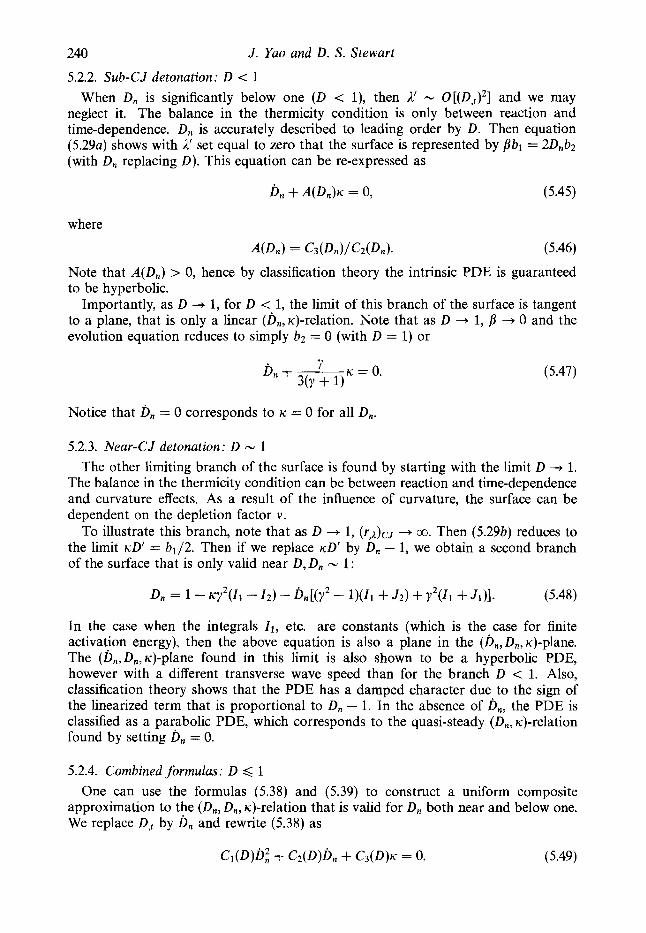
5.2.2. Sub-CJ detonation: D < 1 When D, is significantly below one (D < l), then 1’ - O[(D,t)2] and we may
neglect it. The balance in the thermicity condition is only between reaction and time-dependence. D, is accurately described to leading order by D. Then equation (5.29~) shows with 1,’ set equal to zero that the surface is represented by pbl = 2D,b2 (with D, replacing D). This equation can be re-expressed as
J. Yao and D. S. Stewart
D, + A(Dn)ic = 0, (5.45)
(5.46)
Note that A(D,) > 0, hence by classification theory the intrinsic PDE is guaranteed to be hyperbolic.
Importantly, as D + 1, for D < 1, the limit of this branch of the surface is tangent to a plane, that is only a linear (b,,~)-relation. Note that as D --+ 1, p -+ 0 and the evolution equation reduces to simply b2 = 0 (with D = 1) or
(5.47)
Notice that D,, = 0 corresponds to K = 0 for all D,.
5.2.3. Near-CJ detonation: D - 1 The other limiting branch of the surface is found by starting with the limit D -+ 1.
The balance in the thermicity condition can be between reaction and time-dependence and curvature effects. As a result of the influence of curvature, the surface can be dependent on the depletion factor v .
To illustrate this branch, note that as D + 1, ( r ~ ) ~ ~ + 00. Then (5.29b) reduces to the limit KD’ = b1/2. Then if we replace ICD’ by D, - 1, we obtain a second branch of the surface that is only valid near D, D, - 1 :
In the case when the integrals 11, etc. are constants (which is the case for finite activation energy), then the above equation is also a plane in the (b,,D,,ic)-plane. The (&,D,,~)-plane found in this limit is also shown to be a hyperbolic PDE, however with a different transverse wave speed than for the branch D < 1. Also, classification theory shows that the PDE has a damped character due to the sign of the linearized term that is proportional to D, - 1. In the absence of b,, the PDE is classified as a parabolic PDE, which corresponds to the quasi-steady (D,, ic)-relation found by setting b, = 0.
5.2.4. Combined formulas: D < 1 One can use the formulas (5.38) and (5.39) to construct a uniform composite
approximation to the (D,, D,, relation that is valid for D, both near and below one. We replace D,, by b, and rewrite (5.38) as
C,(D)bi + C2(D)bn + C~(D)K = 0. (5.49)

Dynamics of multi-dimensional detonation 24 1
One can choose a value of D < 1 and K , and then use (5.49) to calculate D,,, or assume a value of D and b,, and use (5.49) to calculate K . Then with the values of b,, K and D fixed, one uses formula (5.29b) to calculate KD' and hence D, = D + KD', thus generating a (b,, D,, Ic)-triad. Thus for a set of equations of state and kinetics parameters, one can generate plots of the (b,, D,, k-)-surface as well as contours in the (D,,~)-plane for fixed D n (say); albeit the required integrals that appear in the formulas must in general be done numerically.
The condition for hyperbolicity, that ( i 3 K / a b n ) D o < 0, must be checked, and the boundaries of this inequality form are used to discard spurious regions and identify the boundaries of the relation. In general, if we solve (5.49) for D,,, we obtain
(5.50)
We have selected the - branch for Al l2 , which is a choice consistent with the requirement of the analysis that b, - o(1). Also, simply from the definitions of C2 and C,, one can show that in the limit as D -+ 1, both CZ, C3 are finite and positive. Thus in an entire neighbourhood of the surface with D = 1 these coefficients are positive. Also one can show that as D + 1, C1 +. -m. Thus the surface must contain the limiting point b, = 0, D, = 1 and K = 0 for D = 1. We take the implicit derivative of equation (5.49) with respect to D,, holding D , fixed (where D, is approximated by D) , and find
(5.51)
Thus we find that the boundaries of the response surface (where the derivative changes sign) are defined by the conditions C2 = 0, C3 = 0, and d = 0. For D < 1, d is strictly bounded from zero, and is approximated by A N 1, for sufficiently small K . However for D - 1, the boundary A = 0 is described by K = C,2/4C1C3.
5.3. Example for a condensed explosive We display the (b,, D,, Ic)-relation for the important cases that can be used to model a condensed explosive. Gaseous explosive mixtures are better modelled by the analysis given in $6. The polytropic (ideal) equation of state is accurate in a quantitative sense only for gaseous mixtures. The use of the polytropic EOS for condensed explosives provides a useful, analytically tractable model that can generate the correct magnitudes for detonation speeds and states; however the equation of state in the unreacted explosive is poorly modelled. The condensed-phase model has been used by us in the past for the purpose of analytical testing of numerical schemes and qualitative predictions about detonation shock dynamics, Stewart & Bdzil (1993).
In order to generate model results for qualitative and numerical testing purpcises for a representative condensed-phase explosive, it is important to choose parameters that reflect the reacted products behind the detonation shock and to display the results in physical units. Representative parameters are y = 3, an initial density PO = 2 g CM-~, a heat of combustion Q = 4 x lo6 J Kg-'. The corresponding CJ detonation speed, from the strong-shock approximation gives bCJ = (2(y2 - l)Q)'I2 = 8 Km s-'. The depletion parameter v is chosen to be 1/2. The pre-multiplying rate constant k" controls the size of a steady half-reaction length, but typically one chooses it to correspond to a typical reaction-zone length in a condensed explosive, which can range from 1/10 to a few millimetres. The value k" = 2 . 5 1 4 7 ~ ~ corresponds to a

242 J . Yao and D. S . Stewart
steady half-reaction-zone length, = 1 mm. When the activation energy B is taken to be zero, the rate integrals, 11,12, J l ,J2 , J can be carried out analytically, and those exact integrals are listed in Appendix D.
Figure l(a) shows a surface plot of the (b,,D,,~)-relation, for the condensed explosive case ( y = 3 , v = 1/2,6 = 0), generated from the formulas of the previous section. The surface is plotted in a space that has D, in the vertical direction, ic in the horizontal x-direction, and D, in the out-of-plane direction. Contours of constant & are shown and labelled in the surface. For all the plots, the half-reaction length is used to scale the curvature.
The surface has a tent shape with a distinct fold near D, = 1, which separates the two branches of the surface, D < 1 and D - 1. The plane b, = 0 intersects the surface along the (D?,rc)-relation for ic > 0. Also the plane intersects the surface along the vertical line D, = 0,rc = 0 for all D,. Thus in the surface, the contour b,, = 0 has a discontinuous derivative exactly at D, = 1. The segment of the surface that is related to the branch D - 1 is completely visible in the surface plot and can be reasonably well-fit by a plane given by the equation
63.6 D, + (D, - 1) + 8.35 ic = 0. (5.52)
The segment of the surface near D, = 1 on the branch D < 1 is well-approximated by the (b,,ic)-relation given by (5.47). The surface is terminated by the edge of the box on the left side of the plot. The lower portion of the surface is terminated by the edge of the box. The left edge of the surface for ic < 0 correspond to the hyperbolic boundary d = 0.
Figure l(b) shows the projection of the surface onto the (D,,ic)-plane, with the contours of D, indicated. For this case, where the activation energy is zero, increasing negative curvature is associated with decreasing values of D,. This is not the case for large activation energy.
5.4. Numerical experiments : diferences between hyperbolic and parabolic evolution Next we present the results of some two-dimensional numerical experiments and comparisons that use (D,, D,, ic)-relations. The numerical solutions of the intrinsic PDEs shown here were carried out in collaboration with T. Aslam, and employ a level-set technique that follows the work of Osher & Sethian (1988). The numerics are described briefly in Stewart et al. (1999, and in detail in Aslam Bdzil & Stewart (1995). The main points to be demonstrated concern the qualitative differences between the detonation shock dynamics predicted by a (b,, D,, K-)-relation and those corresponding to a (D,, rc)-relation, and their prediction of detonation shock dynamics observed in physical experiments.
Our example illustrates the qualitative difference between the hyperbolic (D,, D,, ic)-
relation and the corresponding parabolic (D,, ic)-relation, for the parameters of the condensed-phase model, discussed in 95.3 and illustrated in figure l(a, b). We restrict attention to the branch of the response surface for D - 1, approximated by (5.52). We display the results of the first numerical experiment in length and time units of mm and ps, respectively, and in these units (5.52) becomes
8, = 8 - 66.8R - 7.958, ,
B, = 8 - 66.8R .
(5.53)
with the corresponding (Dn, Ic)-relation
(5.54)

Dynamics of multi-dimensional detonation 243
FIGURE 1. (a) Surface plot of the (D,,D,,K)-relation for the condensed-phase case, with y = 3 , v = 1/2. The curvature IC is scaled with respect to. the half-reaction length. Contours of constant D, are shown and labelled. (b) . Projection of the (D,, D,, rc)-relation to the (Dn, rc)-plane, for the condensed-phase.case. The branch D - 1 is transparent, and the branch D < 1 is shown in grey-scale. Contours of D, are indicated by the labels.
A slab with a half-width of 50 mm and length of 400 mm was used for the experiments. At time t = 0, a plane, CJ shock is assumed at x = 0 mm. Solutions for the shock dynamics in finite domains require boundary conditions to be applied at edges for all time. At the bottom edge ( y = 0 mm), we assumed an angle boundary

244 J. Yuo and D. S . Stewart
FIGURE 2. (b) A solution of the (b,,D,,lc)-relation given by (7.1). The grey-scale records values of D, at a fixed point when the shock crosses it. The first shock position from the left is at 3ps, and the time intervals between subsequent shocks is 3.61 ps.
(a) The solution of the (D,,lc)-relation of equation (7.2).
condition, and in particular the angle between the outward normal of the confining edge and the normal to the shock was taken to be 45". At the top edge (y = 50 mm), the confinement was assumed to be perfect and corresponds to a symmetry (or reflection boundary conditions), and the angle between the outward normal of the confining edge and the normal to the shock was set to 90".
Figure 2(u,b) shows combined contour and line plots that show features of the numerical solution the initial-boundary-value problem defined above. Figure 2(a) corresponds to a numerical solution of the (D,,K)-relation defined by (5.54) and figure 2(b) corresponds to that defined by (5.53). The different greyscale contours, separated by lines that run roughly along the axis of the slab, indicate the value of the detonation velocity recorded at a fixed Eulerian point in the slab, at the time that the detonation shock crosses the point. Dark regions correspond to lower normal detonation velocity and lighter regions higher values. The shock positions are also shown at various times, at equal time intervals of 3.6 p s, and cut transversely the lines of constant d,.
The most obvious difference between the two simulations is illustrated by the relaxation towards an axial steady state of an initial plane-CJ shock, in response to the edge boundary condition applied at y = 0 mm. The relaxation of the solution (D,, K-)-relation from plane-CJ to its axial, steady-state in response to a step change in slope is via local, self-similar relaxation, characteristic of the heat equation. This is seen in the curves of constant dn where, y cc x ' / ~ . In contrast, the hyperbolic character of the solution to (5.53) is seen by the curves of constant d, with y cc x that are the consequence of the self-similarity of the local wave equation that governs the early transient. Also the relaxation for the (D,, Ic)-relation, shown in figure 2(a), is accomplished quickly in the first 100 mm (say), while an obvious transient still persists in the solution of the (b,, D,, K-)-relation, even at 400 mm, four slab thicknesses wide.

Dynamics of multi-dimensional detonation 245
The constant-D, contours show evidence of multiple wave reflections of the initial disturbance off the confinement boundaries. The shapes of the axial, steady shock loci are different in the two cases, which is due to the effects of the normal acceleration, &.
6. The limit of large activation energy and small curvature and slow evolution
In this section we separately consider a distinguished limit of large activation en- ergy and small curvature and slow evolution, suitable for the description of a gaseous, pre-mixed explosive with a sensitive reaction rate. We relax the strong-shock approx- imation that is used in $5, and instead use the general shock relations. Ultimately, we derive an intrinsic equation of a more complex form, F(B,,bn,D,,~,k) = 0, by means of two successively applied iterations that determine corrections to the steady plane CJ detonation structure. This equation, when plane, with IC = k = 0, reduces to a (b,, b,, D,)-relation, which is a second-order ordinary differential equa- tion. It will be shown that this ODE admits a simplified stability theory, and has a neutral stability boundary in an ( E , Q)-plane, which corresponds asymptotically to the exact linear stability curve calculated in Lee & Stewart (1990). The same ODE also admits limit-cycle pulsations that correspond to those first found nu- merically by Fickett & Wood (1966), in the numerical solution to the reactive Euler equations.
When multi-dimensional solutions are considered, this new relation is an intrin- sic PDE: a nonlinear wave equation. For reasonable sets of physical parameters, corresponding to gases, the PDE contains a hierarchy of hyperbolic wave families. The lowest-order family is simply the first-order hyperbolic PDE that corresponds to Huygen’s construction, D, = 1 ; the second corresponds roughly to a b,, K pairing, and the pairing of the highest-order derivatives of b, and ic corresponds to the wave operator that controls the type of the equation. We have found, in collaboration with T. Aslam, that this PDE admits cellular dynamics for the motion of the detonation shock, and that the dynamics and cell growth of the solution are remarkably similar to those observed in the physical experiments.
To explain this further, we mention some aspects of the observations of multi- dimensional detonation cells in experimental systems, such as those observed by Strehlow et al. (1967) in dilute hydrogen-oxygen explosive mixtures. In a typical experiment, a long rectangular channel is used to contain an unreacted explosive mixture of hydrogen/oxygen gas, diluted by argon (say). The mixture is ignited at a closed end and is allowed to propagate down the tube. As it propagates, the detonation shock, instead of being plane, has a set of disjoint cells, which are made up of segments of the detonation shock that travel at different normal velocities, and correspond to quite different shock pressures. The segments of the detonation shock are resolved by shock/shock interactions that may be regular, or may lead to Mach-stem formation and growth. In the case of a regular reflection, the triple point remains, while in the case of Mach-stem growth, the point of interaction becomes two triple points connected by a bridge that grows in width. Thus the cellular detonation shock front can be characterized simply as a network of triple points that are connected to smooth shock fronts.
In the physical experiment, the inside of the tube is lined with foil that is covered with soot, typically from kerosene burned in air, which is partially scraped away by the high-pressure detonation shock that intersects the tube wall. In particular, the loci of the wall motion of the shock triple points are easily recorded by the smoke-foil

246 J . Yao and D. S. Stewart
technique. In the foil one sees the characteristic patterns enscribed by the motion of the triple points. We find that remarkably similar patterns are generated by solution of the (b,, D,, D,, IC, k)-intrinsic PDE, that we derive here.
Thus we find that a single evolution equation, of hyperbolic character, can describe many features of the motion of the cellular detonation front. The new intrinsic PDE admits weak solutions with continuity of the shock locus, but with discontinuities in the shock slope. The points of the intersection, where the shock slope is discontinuous, between different otherwise smooth shock segments correspond to the location of triple points in a numerical experiment. These points moved from side to side on the shock front as the shock moved forwards. When the triple points collide with the side wall, they are reflected back into the channel, as would be expected in the physical experiment. For many of the numerical experiments we tried, cells would form quickly and the number of cells (counted from the patterns that the triple points made as they propagated down the channel) would persist. However by varying the spatial frequency of the initial sinusoidal shape of the shock and the initial velocity, we almost always found that the frequency of the initial data was not preserved. Indeed, as in the physical experiments, the cells actually absorb other cells, and generate larger cells as time evolves. These larger cells then persist and are self-sustained.
For large activation energy the reaction zone is an induction zone, followed by a thin heat-releasing reaction zone. The analysis that follows is motivated from our previous work in Yao & Stewart (1995), where we calculated the (D,, Ic)-relation in the absence of any additional time dependence. There we assumed that the small curvature is measured on a typical induction-zone length scale for the plane-CJ detonation, and is specifically O(l/O) on that scale. Deviations of the normal detonation velocity of O(D, - 1) were assumed to be of the same order; and as a consequence, the analysis showed that the (D,,K)-relation is multi-valued in D, for a limited range of K , and that a critical pair [(Dn)cr,~cr] exists such that for IC > xCr, no asymptotic solution of this type exists. Importantly, this calculation employed matched asymptotic layer analysis. A similar analysis, rigorously done, that also uses matched asymptotics and not an ad hoc analysis was recently carried out by Klein, Kroc & Shepherd (1995).
Unlike the above-mentioned calculations, we use the MSA technique, and work with the integrated form of the problem. Some additional features of this calculation should be explained as background, in advance of the presentation of the details. In the case of large activation energy, since the reaction can change by an 0(1) amount in response to a temperature (sound speed) perturbation of O(l/O), one must necessarily calculate the effect of the temperature perturbations explicitly in a well-defined induction zone (IZ); and the IZ is near the shock. At the same time, the integration must be carried out approximately all the way to the generalized CJ point. So it follows that if one uses the reaction coordinate, 1, as the independent variable, in place of n, one integrates from 1 = 0 to 2 = 2cJ, and the induction zone is accounted for explicitly as a region of small reaction depletion by the introduction of a scaled reaction progress variable, A = z/O.
Because of the use of 1 as the independent spatial-like variable, the integrals that appear on the right-hand side have the inverse reaction rate r-] in the integrand. As one leaves the IZ, the region of small depletion, towards the region of large heat release, the fire, the reaction rate become exponentially large, and many of the integrals that appear have exponentially small contributions in the fire region. The fact of this exponential convergence, reflecting the stiff tightly organized fire region, which in reality has a very simple structure, makes approximating the structure with

Dynamics of multi-dimensional detonation 247
two iterations tractable, since one can carry out the indicated integrals largely by using IZ approximations.
In a sense, the fire remembers the events of the induction zone and follows it. The induction zone and the fire, however, retain their separate identities, in that the velocity of the fire relative to the shock comes out explicitly as the time derivative ACJ, as in equation (5.6), through the application of Leibnitz’ rule. (Note that when we refer to a time derivative, a/atl,, that later must be interpreted as an intrinsic normal time derivative, we use the dot notation, interchangeably).
To carry out the calculation using the MSA technique, one only has to assume that at each level of iteration one adds higher-order corrections, with successive iterations. As one carries out the iteration, one has the option to drop terms that are deemed higher order, for the purpose of simplifying the calculation, and indeed this is a rational procedure provided one stops at a certain order in the calculation. Again the MSA procedure is entirely similar to a numerical approach used to solve the steady ODES described in Yao & Stewart (1995).
The specific sequence of the iteration is important in order to efficiently carry out the calculations that yield the final intrinsic PDE. The one that works well generates the steady (D,,K)-relation with the turning point in the first iteration and was determined as follows. The zeroth iteration is the one-dimensional steady CJ, zero normal derivative solution. This solution does not depend on time and hence does not generate time derivatives when constructing approximations to the terms on the right-hand side of the PDE. One does generate the terms associated with the curvature corrections on the right-hand side. However it is not accurate enough to simply use the zeroth-order solution to estimate the inverse reaction rate, prior to the computation of the integrals. Indeed the greatest contribution to the integrals in 1 is in the IZ, for 1 N O(l/O). In particular, the reaction rate itself is a function of the perturbed temperature which in turn is a nonlinear function that must be calculated. This is done by carrying out a separate IZ calculation to determine the perturbed temperature, and hence the rate, in terms of the small amount of reaction. The weight of the integrals is then changed by accounting for the spatial corrections to the reaction rate induced by the IZ.
With the improved estimate of the reaction rate r , the calculation of the integrals, with their dominant contributions from the IZ, can be carried out easily, and indeed the nearly conservative form of the equations yields corrected RH-relations that have explicit dependence on both scales 1 = z/O with z - 0(1), and 1 - O(1); the former is on the scale of the induction zone and the latter on the scale of the fire. Of course in the integral treatment, the layers that would be present in a matched asymptotic treatment are automatically matched, since the integral technique automatically generates composite expansions. The steady (D,, rc)-relation in fact can be obtained after the first iteration, if desired, by suppression of an apparent singularity as 1 + 1.
Having completed the first iteration, one has introduced time dependence in the corrections by exact application of the shock conditions, in terms of D,. In computing new approximations to the right-hand side, D, - 1 and D, appear explicitly. But importantly at this stage, explicit consideration of the effects of acceleration of the shock is introduced. The second iteration involves corrections to the IZ, and a new estimate for the temperature perturbation, which in turn give an improved estimate of the reaction rate in the IZ. The corrected IZ solution and the corrections to the rate allows one to compute improved corrections to the integrals, and ultimately new corrections to the RH-relations. Finally, D, and the appearance of k occur, roughly
248 J. Yao and D. S. Stewart
speaking, through the calculation of the time derivative of ncJ, or the velocity of the fire, relative to the shock. The evolution equation is finally computed by using the solution to the RH-algebra to estimate the values of the states at the generalized CJ-point and then substituting the result into the sonic condition and thermicity conditions.
One can interpret this analysis as an exercise in low-frequency nonlinear acoustics, where one has explicitly accounted for the lowest fundamental acoustic modes. Since two refined iterations are carried out to generate approximate solutions to the full Euler equations, a fairly large number of terms associated with D,,,Ic and their derivatives are generated and must be kept and finally collapsed into a surface relation. The derivation of the new intrinsic PDE follows next. The algebra is extensive, but we have made every attempt to make the procedure clear. But some details are necessarily left to the reader. Additional information is available in Yao’s (1996) thesis.
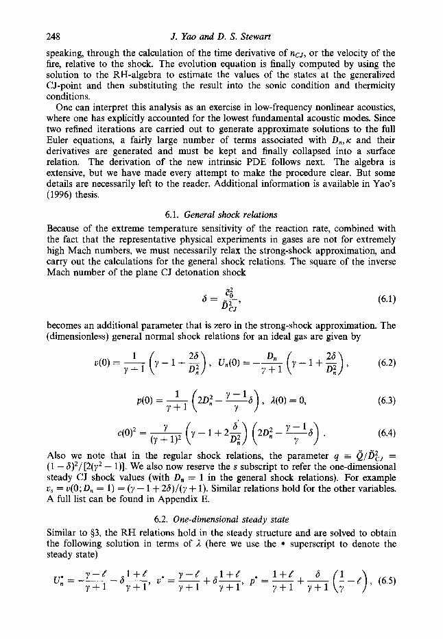
6.1. General shock relations Because of the extreme temperature sensitivity of the reaction rate, combined with the fact that the representative physical experiments in gases are not for extremely high Mach numbers, we must necessarily relax the strong-shock approximation, and carry out the calculations for the general shock relations. The square of the inverse Mach number of the plane CJ detonation shock
z; @-’
a = -
becomes an additional parameter that is zero in the strong-shock approximation. The (dimensionless) general normal shock relations for an ideal gas are given by
P(0) = y+l 1 (ZD: - - y%), A ( O ) = O , Y
C ( O ) ~ = L (Y + (y--1+2$) (2D’-- - Y 18)
Also we note that in the regular shock relations, the parameter q = Q/& = (1 - S ) 2 / [ 2 ( y 2 - l)]. We also now reserve the s subscript to refer the one-dimensional steady CJ shock values (with D, = 1 in the general shock relations). For example us = u(0; D, = 1) = ( y - 1 + 26)/(y + 1). Similar relations hold for the other variables. A full list can be found in Appendix E.
6.2. One-dimensional steady state Similar to 93, the RH relations hold in the steady structure and are solved to obtain the following solution in terms of 2 (here we use the * superscript to denote the steady state)
U ’ - y - - e I + [ t Y - - e 1 + e * 1+e 6 + 1 + Y + l y + l y + l y + 1 ’ =- -[) 9 (6.5) 6-, 0 =- +a-
Dynamics of multi-dimensional detonation
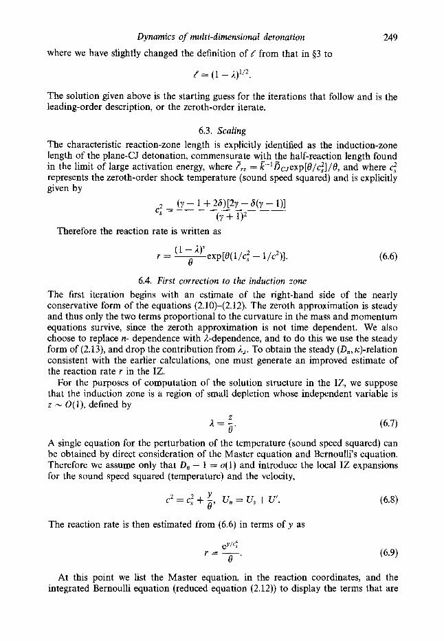
where we have slightly changed the definition of h' from that in $3 to
249
e = (1 - j1)1'2
The solution given above is the starting guess for the iterations that follow and is the leading-order description, or the zeroth-order iterate.
6.3. Scaling The characteristic reaction-zone length is explicitly identified as the induction-zone length of the plane-CJ detonation, commensurate with the half-reaction length found in the limit of large activation energy, where z,, = k"-1bcrexp[8/c~]/0, and where ct represents the zeroth-order shock temperature (sound speed squared) and is explicitly given by
Therefore the reaction rate is written as
6.4. First correction to the induction zone The first iteration begins with an estimate of the right-hand side of the nearly conservative form of the equations (2.10)-(2.12). The zeroth approximation is steady and thus only the two terms proportional to the curvature in the mass and momentum equations survive, since the zeroth approximation is not time dependent. We also choose to replace n- dependence with A-dependence, and to do this we use the steady form of (2.13), and drop the contribution from A,t. To obtain the steady (Dn, rc)-relation consistent with the earlier calculations, one must generate an improved estimate of the reaction rate r in the IZ.
For the purposes of computation of the solution structure in the IZ, we suppose that the induction zone is a region of small depletion whose independent variable is z - O( l), defined by
A = - 0 '
A single equation for the perturbation of the temperature (sound speed squared) can be obtained by direct consideration of the Master equation and Bernoulli's equation. Therefore we assume only that D, - 1 = o( 1) and introduce the local IZ expansions for the sound speed squared (temperature) and the velocity,
(6.7) Z
(6.8) 2 2 Y c = c, + -, un = us + U'.
0
The reaction rate is then estimated from (6.6) in terms of y as
eYl4 r = -
0 .
At this point we list the Master equation, in the reaction coordinates, and the integrated Bernoulli equation (reduced equation (2.12)) to display the terms that are

250
retained in the local IZ description, as
J. Yao and D. S . Stewart
au Un (c2 - V , ' ) L = [qr(y - 1) - I C C ~ ( U , + D,)] -, r an
D2 6 qR = + -, u; c2 2 7 - 1 2 y - 1 -+--
(6.10)
(6.11)
An equation for y is obtained simply by differentiating Bernoulli's equation (6.1 1) with respect to A, using the result to replace the derivative aU,/aA in the Master equation, followed by the use of the approximate expansions introduced above. The boundary condition for y comes from the linearization of the shock boundary conditions. One obtains the following problem for y :
subject to the boundary condition that
y = pc39(D, - 1) at z = 0,
(6.12)
(6.13)
where the definitions of constant parameters a,p, and p are in terms of shock-state values and q, and are given here in terms of y and 6 as
1 - 6 [3y - y? - S(3y - l)], p = 2- (y - l) [2y - S ( y - l)](y - 1 + 26)2,
c( = 2(y + 1)2 (Y +
(6.14)
The solution for y can be written succinctly as
(6.15) a2
y / c : = pe(D, - 1) + - + Y , 4
where
9 = In 1 + - e-az/c;)e-MVDn-l) (6.16) 1 Y" The reaction rate can now be expressed using the solution just given for y as
az/c:+@(Dn-l)+.Y (6.17) r = e e The solution for the first approximation in the IZ can now be expressed as
I 1 1 - 6 d
2 y + l 1 1 - 6 d
un = U,(O) - -----A + $9,
V = V(0) + --A - -9, 2 y + i e
c4 c2 = C ( O ) 2 + an + 29, e
(6.18)

Dynamics of multi-dimensional detonation
where ~7 is a constant defined by
25 1
(6.19)
If desired, one can now simply generate a composite solution through the fire zone, by integrating the right-hand side of the quasi-conservative equation with respect to the independent variable A, which we indicate as
(6.20)
One uses the above definition of (&)-l in the IZ, from (6.17), and carries out the indicated integrals. The relations now represent modified RH-relations, which can be solved approximately to first order in the perturbations to obtain composite expansions of the form
where
(6.23)
The steady (Dn, Ic)-relation found in Yao & Stewart (1995), for example, is obtained by suppressing the singularity that otherwise would appear as t + 0, and by setting h(z = co) = 0. One can easily verify that the condition leads to the result
where the coefficients a, b and d are defined by
(1 + W Y - ll(Y + ( Y + 4[2y - S ( y - 1112’
(Y - ll(Y + U3[3Y - 1 + 6(3 - 711 = (y + S)(y - 1 + 2S)2[2y - S(y - 1112’
a =
4(Y - l ) (y - 1 + 26)2(2y - y6 + 6) d = (1 - S) (Y + 1)’[3~ - y 2 - S(3y - l)]’
(6.24)
k (6.25)

252 J . Yao and D. S. Stewart
6.5. Second correction to the induction zone Now we use the induction-zone approximations from the first iteration to system- atically add the effects of unsteadiness to the description of the IZ. Note that the first approximation now explicitly includes quasi-steady time dependence through the appearance of both D, and IC. Upon differentiating with respect to time the first approximation, and using the result in the right-hand side of the nearly conservative form of the governing equations, one adds the derivatives D,, = b,, and IC,, m k. Also since we use the reaction coordinate as the independent variable, we use the corrected change of variable, dn = U J ( r - must be computed. We consider this estimate next.
Starting with the integrated definition, n = Jt U , / ( r - A,t)dX, further differentiation with respect to t holding n fixed gives
and an estimate of
(6.26)
where we assume that N o(r), and use the IZ approximations from the first iteration for r from (6.17). Carrying out the indicated differentiation and integration, gives the estimate for A,,
A ,t - - cIc,i)n(eaz/c: a - 1). (6.27)
At this level, one can compute additional corrections to A,t, but later these terms are time differentiated or multiplied by other small terms, and we can neglect those contributions.
In the differentiations that follow, we also encounter the derivative, 9,t In, which is calculated from the definition of 2' and the chain rule formula, Y,tIn = 2 , t I i + 9 , n I t A , t . One finds the estimate
2,t[, = 53. (6.28)
In what follows we make the explicit assumption that k N o(b,) , hence we have that Y,tI,/O - o(&), and we use that to simplify the next set of approximations.
The second iterated corrections to the structure of the IZ are based on using the results of the first iteration to estimate the various time-derivative terms in the right-hand side of the nearly-conservative form of the governing equations, and then expressing the result in terms of the corrected Master equation and Bernoulli's equation, in the scaled IZ reaction coordinate, z = 16. One again needs to be particularly careful in expressing the reaction rate in the IZ, due to the exponential sensitivity of the rate on the temperature. For example the following ratio that appears in the change of variable is expressed approximately as I/(r--&) = r - l ( l + l , t / r ) . Again one obtains a correction to the sound speed squared represented by c2 = cf + y /O , and derives an equation for y. This can be done directly since we drop terms in the resulting equation for y that are O(l/02). The approximate Master and Bernoulli's equation that we use to compute the second IZ corrections are listed as
4
K
P u n (6.30)

Dynamics of multi-dimensional detonation 253
In Bernoulli's equation, we can use the approximation in its right-hand side that
C2 - + - - qA] = D,&. [Y y - 1 ,t
(6.31)
For convenience we define the time-dependent terms that appear on the right-hand side as
H = Un( Un,t + Bn) - V P , ~ , G = uP,t - bn( Un + D n ) . (6.32)
Then using the first-iteration IZ approximations, we can obtain approximate expres- sions for H and G as
(6.34) 2[y - 3 + ( 5 + y)6] .
G = Dn - (1 - 6)(y - 1 + 26)
4 t . 2(Y + (Y +
Thus we can recast the revised Master and Bernoulli's equations as
(6.36)
As in the first iteration, one uses Bernoulli's equation to obtain an approximate expression for aU,/aA, and substitutes into the Master equation to obtain a new approximate equation for y, where the reaction rate can be approximated again with (6.17). The new equation for y becomes
subject to the shock boundary condition
y = p c % O ( ~ , - 1) at y = 0,
where
+ ple& + P26J,t + o(q t ) .
The new parameters are defined by
(6.38)
(6.39)
(6.40)
( y - 1 + 26)2(3 + 6) (Y +
Y - 1 2 8 2 = - 3 % .
254 J . Yao and D. S . Stewart
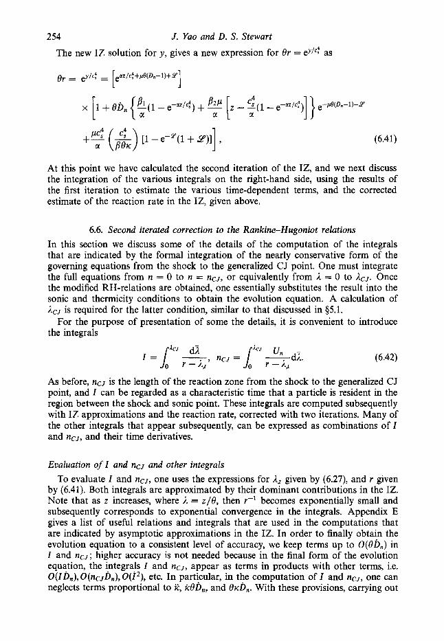
The new IZ solution for y , gives a new expression for Or = eyjc; as
(6.41)
At this point we have calculated the second iteration of the IZ, and we next discuss the integration of the various integrals on the right-hand side, using the results of the first iteration to estimate the various time-dependent terms, and the corrected estimate of the reaction rate in the IZ, given above.
6.6. Second iterated correction to the Rankine-Hugoniot relations
In this section we discuss some of the details of the computation of the integrals that are indicated by the formal integration of the nearly conservative form of the governing equations from the shock to the generalized CJ point. One must integrate the full equations from n = 0 to n = ncJ, or equivalently from A = 0 to AcJ. Once the modified RH-relations are obtained, one essentially substitutes the result into the sonic and thermicity conditions to obtain the evolution equation. A calculation of LCJ is required for the latter condition, similar to that discussed in $5.1.
For the purpose of presentation of some the details, it is convenient to introduce the integrals
(6.42)
As before, ~ Z C J is the length of the reaction zone from the shock to the generalized CJ point, and I can be regarded as a characteristic time that a particle is resident in the region between the shock and sonic point. These integrals are computed subsequently with IZ approximations and the reaction rate, corrected with two iterations. Many of the other integrals that appear subsequently, can be expressed as combinations of I and ncJ, and their time derivatives.
Evaluation of I and ncJ and other integrals
To evaluate I and ncJ, one uses the expressions for A,t given by (6.27), and r given by (6.41). Both integrals are approximated by their dominant contributions in the IZ. Note that as z increases, where A = z/O, then r-l becomes exponentially small and subsequently corresponds to exponential convergence in the integrals. Appendix E gives a list of useful relations and integrals that are used in the computations that are indicated by asymptotic approximations in the IZ. In order to finally obtain the evolution equation to a consistent level of accuracy, we keep terms up to O(eb>, ) in I and ncJ; higher accuracy is not needed because in the final form of the evolution equation, the integrals I and ncJ, appear as terms in products with other terms, i.e. O(Ib , ) , O(ncJb,), O(Z2), etc. In particular, in the computation of I and ncJ, one can neglects terms proportional to R, kOb>,, and ercb,. With these provisions, carrying out

Dynamics of multi-d imensional detonation 255
approximations to the integrals I and ~ Z C J gives
and
where
where
(6.45)
and where Un(0) is the exact value of Un at the shock, and hence is defined in terms of Dn by (6.2b).
Next we approximate the integrals and terms that arise from the integration of the right-hand side of the nearly-conservative equations from the shock to the CJ-point. Note that the naming convention used here is to reserve the 9 for the integrals for the two curvature terms that appear in the older quasi-steady theory, 9 1 , 9 2 (in the absence of the explicit time derivatives), and to use f , for the integrals that arise from the time-dependent terms. Also in the expressions for f l and $3, we show the result of the application of Leibnitz' rule, which accounts for the fact that we integrate to ncJ (in order to apply the generalized CJ conditions) and which shows the explicit appearance of the velocity of the fire relative to the shock, hCJ. We list these below for (re)naming purposes, for clarity and to indicate the calculations that follow :
Pelc -@(Dn-1) Y ~ J = Y(z = 00) =In 1 + -e l a
(6.46)
- D,, pdii = DnI + . . . , (6.51)

256 J. Yao and D. S. Stewart
- + - - qR dii = -DJ + .. ., 2 y - 1
n C J
- D,, 1 dfi = -DflncJ.
(6.52)
(6.53)
As an example of how to continue to further approximate these integrals, we first discuss the computation of $1. Use the first IZ approximation for p , change variable from n to 1, approximately compute the integral, followed by the differentiation of the result. Terms in the integral are retained to O(&) and O(ic), which gives the following approximate formula:
The integrals 91~92 are estimated in terms of I as
.... 1 - 6 Y + l
(Y - 1 + 26II +
(Y + 91 = 2K-I + * . . ., $2 = 2 K ( 1 - 6)
(6.54)
(6.55)
The integrals $ 2 , 2 3 can be computed in a similar fashion to f l , and are approxi- mated by
Formal integration and Rankine-Hugoniot algebra Now, we can express an approximation of the integration of the nearly conservative
form of governing equations to the generalized CJ point. Directly expressed in terms of the previous integrals, we find the following modified RH-relations at the generalized CJ point (similar to (5.10)-(5.12):
where c : ~ = ~ P C J / ~ C J . The object now is to solve for the CJ states, pcJ, (U&, P C J , &--, subject to the constraint of the sonic and thermicity conditions at the CJ point. Therefore it is necessary to solve the algebra explicitly for that purpose. Note further,

Dynamics of multi-dimensional detonation 257
that pcJ, (pU,)cJ and pcJ appear both on the left- and the right-hand side of the modified-RH relations, through the definitions of
We explain a simple procedure for inverting this algebra. First, exhibit all the explicit CJ-dependence, some of which appears in the integrals on the right-hand side. Then manipulate the algebra to obtain an explicit equation for ( u , ) ~ . The other states follow simply. To do this, we use the definitions of the integrals, 91,$2,$1,$2,$3,
in terms of I and ncJ and their time derivatives, and by direct substitution one can rewrite the relations to exhibit the CJ states as
$2, f 3 .
(U%J 2
where the intermediate formulas as
(6.63)
variables R1, R2, R 3 are found by comparison with the previous
(6.64)
(6.66)
Note that by writing the modified RH-algebra in this way, we have displayed the constants associated with the shock and the quasi-steady integrals and the CJ-states explicitly.
The next step is to obtain an explicit equation for (Ufl)cJ, as follows. First substitute ( ~ c J ( U , ) C J + D,) from (6.61) into (6.62). Next, divide the resulting equation (6.62) by ~ C J and replace ~ C J / ~ C J by & / y . The sonic condition can then be used to replace c$,/Y by ( V ; ) C J / ~ . The density p c ~ still remains in this reduced momentum equation, but it can be replaced in the mass equation (6.61) to obtain an equation that is quadratic in ( U,)O :
So far, we have only used the mass and momentum equations and the sonic condition to obtain (6.67), and we have not yet used the energy equation. This quadratic can be solved directly for ( U J C J , as a perturbation from the steady one-dimensional, solution, (UfljlJ = - [ y / ( y + 1)](1+ 6 / y ) :

258 J . Yao and D. S . Stewart
We notice further that we can get an expression for pcJ from the mass and momentum as follows. By using the substitution (Un)cJ = C& = ypCJ/pc~ in the momentum equation (6.62), using the mass equation (6.61) to eliminate PCJ in favour of ( U n ) i J , and discarding terms assumed to be higher order than it$J, one obtains for PCJ
] (6.69) 6
P C J = - [.n + 5 + ( P & ~ C J + 91 + R I ) ~ C J + R2 - 9 2 . Y + l
We now write down the CJ-states at the sonic locus which are summarized below. For the purpose of comparison with the result of §5 (5.20), we define the intermediate variables S1 to SS as
1 + 1 ($1 + Rl)]. (6.73) s6 = -
Then the CJ states can be represented as
+ Dn 2s2)] + S4, (6.74)
(6.76)
Again c i J can be obtained from the product Y P C J U C J or ( Un)iJ.
the sonic condition) into the energy equation to obtain Next we substitute the results of the CJ states (which have already been employed

Dynamics of multi-dimensional detonation 259
(6.77)
Note that there is a direct correspondence of terms in conditions (6.77) and (5.20). The terms 9 1 and 9 2 correspond to Ilic and I~Ic, respectively. The term S1 correspond to Ilbn, S2 corresponds to J1bn and S, corresponds to J 2 D n . Similar to the result in $5 (5.20), the last equation is a relation between f i n , bn, D,, IC, ri: and ICJ . An analysis of the thermicity condition gives the remaining condition on IcJ.
6.7. The thermicity condition and the calculation of IcJ As in $5, the last step toward the evolution equation is the calculation of IcJ, which follows from the thermicity condition (2.16). We start with the thermicity condition to leading order (corresponding to (5.24)), written as
(6.78)
where (t,t)cJ = - ( I , t ) ) ~ ~ / ( 2 d c J ) follows from the definition of e used here: e = (1 - A)'/'. In turn, (I,)cJ follows from the formula (similar to the result (5.36))
(6.79)
This formula is used in the previous expression for the leading-order thermicity condition to replace and we note that the factor of rcJ is common to all terms and can be divided out. What remains is a formula that allows us to compute dc-, hence ACJ, which is written schematically as
(6.80)
In the above expression we have used the shock value for (?J& that would appear in the integrand, and subsequently the integral indicated is approximated as well using the IZ approximation for r , from formula (6.41). Carrying out the integral approximately yields the following approximation for ICJ :
(6.81)
6.8. The form and properties of the evolution equation The final step is to insert the formula for ICJ into (6.77) and use the definitions of S1 - Sg, to write a wholly contained intrinsic evolution equation for the detonation shock surface in terms of bn,bn,Dn,rc and k. The algebra of reconstitution is straightforward, but is very lengthy due to the large number of terms that generated in the two iterations. However to reveal character of the evolution equation further,

260 J. Yao and D. S . Stewart
and to present a simplified form of it, we simplify many of the coefficients and terms that define S1 -S6 by their limiting form for vanishingly small curvature. For example, by use of the definition of YcJ in (6.45), we obtain the replacement
which in turn can be used to simplify the expressions for ncJ, and I , and their time derivatives, and like terms. Specifically in the case of the terms in (6.77), which limit to the steady (D,, Ic)-relation of the older theory, we retain the logarithmic dependence on the curvature contained in YcJ with the specific simplification
(6.83)
where Cg is a constant that only depends on y and 6 and is defined in Appendix E. Using this simplifying limit of small curvature, for fixed D, and derivatives, we find that (6.77) with ICJ as given by (6.81) can be reduced to the following simplified equation:
where C1 - C8 are all material constants, defined by their values of y and 6. Again, Appendix E gives the set of explicit formulas that show their dependence on the parameters y and 6. Note that the parameter dependence on the scaled activation energy &dependence is shown explicitly.
Importantly, this form of the evolution equation contains the most important features that we need to point out. In the absence of the derivatives of D,, i.e. small b,,, and b,, the steady (D,,K)-relation obtains. In the absence of curvature, both gCJ and k are zero, and the evolution equation reduces to a second-order nonlinear ordinary differential equation, whose stability theory for the stationary solution D, = 1, corresponding to the plane CJ detonation, is found to be asymptotic to the exact linear stability of plane detonation. This result provides, of course, an important check of the entire procedure, and verifies the means by which we have calculated the terms that we have discussed. Nonlinear solutions of the same ODE exhibit limit cycles and correspond to pulsating detonation. Finally in the case where we keep both curvature and time dependence, one must solve an extremely nonlinear scalar wave equation, which has been done numerically in a case that corresponds to self-sustained cellular detonation propagation. We give examples of all three special cases next.
6.8.1. The steady (Dn, K)-relation When time dependence is absent, the evolution equation (6.84) is simplified as
(6.85)
which can simply be shown to reduce to the formulas (6.24) which is exactly the same as the steady (D,,~c)-relation with a turning point obtained by the layer matching method (Yao & Stewart 1995).
9 C J D, - 1 + C 6 7 - = 0,

Dynamics of multi-dimensional detonation 261
6.8.2. One-dimensional dynamics and pulsating detonation
ordinary differential equation, namely When the wave is flat, and IC = k = 0, then (6.84) reduces to a second-order
Indeed this ODE is a nonlinear equation for the dynamics of a near-CJ plane detonation that takes explicitly into account the first effects of low-frequency acoustics. This ODE has a stability theory for the CJ detonation D, = 1 that is asymptotic to the exact linear stability theory, as calculated in Lee & Stewart (1990).
Local linearization of (6.86) at the fixed point (D, ,b , ) = (1,O) leads to a linear ODE that corresponds to a linear oscillator with damping. Let x = D, - 1; we obtain
c,eR + (c2e + c3)n + = 0. (6.87)
It is easy to show that C1 > O,C2 c 0, and C3 > 0, for reasonable values of y and 6. Therefore when 8 > IC3/C21, we have an oscillation with negative damping, the solution is unbounded as time increases, and the detonation is unstable. When 8 < IC,/C2l we have an oscillation with positive damping, and the CJ state is stable. The stability boundary is given by
(6.88)
When y in particular is fixed, then this condition is a relation between 6 and 8, or equivalently, between Q and E . In order to make a comparison with the ex- act result computed from linear stability theory, found in Lee & Stewart (1990), we note that there, a C-shaped neutral stability boundary for f = 1 (i.e. CJ) is plotted in Erpenbeck‘s scaled activation energy, E , and scaled heat of combus- tion Q. The relation between our parameters and Erpenbeck‘s is simple and is given by E = 8/6, Q = y(1 - 6)2/[2(y2 - 1)6], so that we can make a direct comparison.
Figure 3 shows the comparison. ‘Lee & Stewart’ is the label for the exact linear stability calculation, and ‘Yao and Stewart’ labels the plot of the condition (6.88) calculated with the formula from Appendix E. For both curves to the left of the neutral stability curve, for lower values of the activation energy E,(8) , and fixed Q, the detonation is one-dimensionally stable. To the right of the neutral stability curve, for higher values of the activation energy E,(8) , and fixed Q, the detonation is one-dimensionally unstable. Note that only the bottom branches (for lower values of Q) should be considered in the asymptotic comparison, since on the upper branch it can be shown that (6.88) corresponds to finite limiting value of 8, as Q and E are increased. The bottom of the C-shaped curve is asymptotic to the exact result, and 8 -+ GO as E is increased without bound. Interestingly, the formula (6.88) qualitatively predicts correctly the entire C-shape, which might have been unexpected.
One can also show easily, directly from (6.86), that for activation energies slightly higher than the critical neutrally stable activation energy, a stable limit cycle is predicted. Figure 4 shows an example of the numerical solution of (6.86), for the

262 J. Yao and D. S. Stewart
1000
100
1
0.1 0 20 40 60 80 100
E
FIGURE 3. Comparison of the asymptotic neutral stability boundary in the ( E , Q)-plane, represented by (6.88), with the line labelled as ‘Yao & Stewart’ versus the exact linear stability theory labelled ‘Lee & Stewart’, for y = 1.2.
Dn
1.1
1 .o
0.9
0.8
0.7 1 1 I i I I I I I I 1 -2 - 1 0 1
Dn FIGURE 4. Plot of the solution trajectory of (6.86) in the (b,,D,)-phase plane, for
E = 9 , Q = 5 0 , y = 1.2.
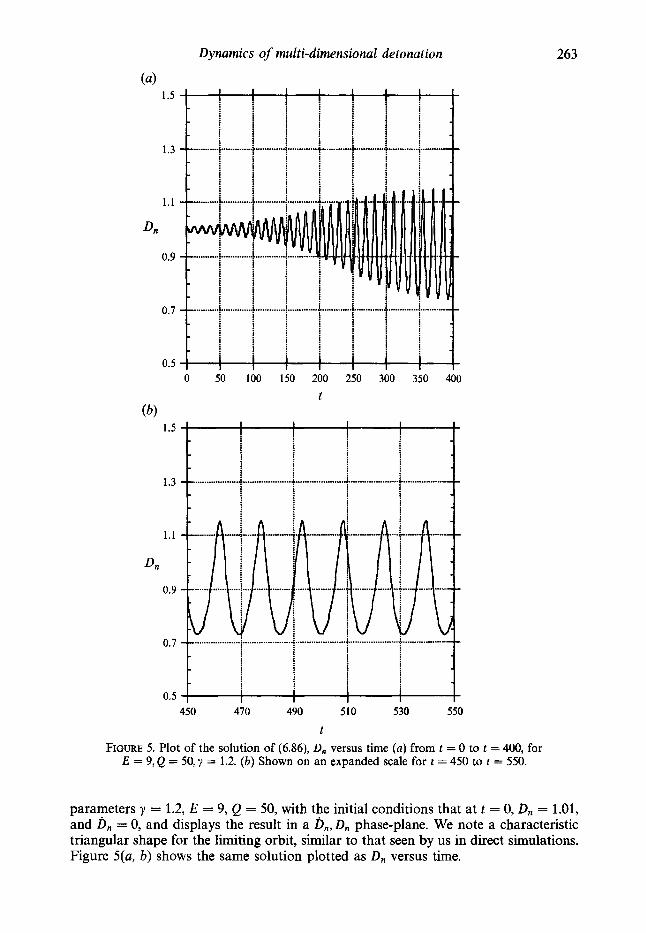
Dynamics of multi-dimensional detonation 263
1.5
1.3
1.1
DII
0.9
0.7
0.5 0 50 100 150 200 250 300 350 400
t (b)
1.5
1.3
1.1
Dn
0.9
0.7
0.5 450 470 490 510 530 550
t FIGURE 5. Plot of the solution of (6.86), D, versus time (a) from t = 0 to E = 400, for
E = 9, Q = 50, y = 1.2. (b ) Shown on an expanded scale for t = 450 to t = 550.
parameters y = 1.2, E = 9, Q = 50, with the initial conditions that at t = 0, D, = 1.01, and D, = 0, and displays the result in a D,, D, phase-plane. We note a characteristic triangular shape for the limiting orbit, similar to that seen by us in direct simulations. Figure 5(a, b) shows the same solution plotted as D, versus time.
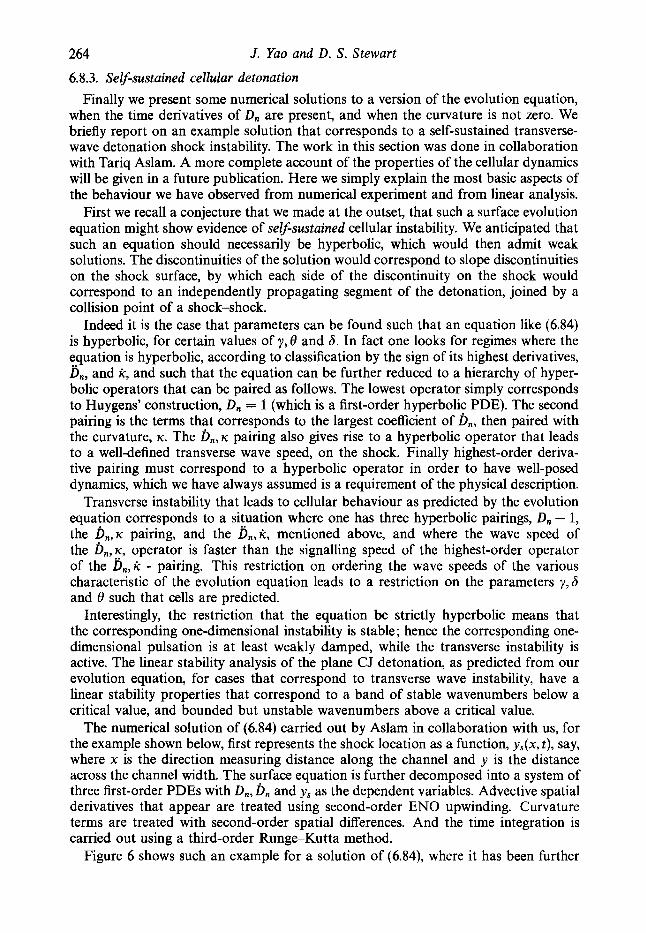
264
6.8.3. Self-sustained cellular detonation
Finally we present some numerical solutions to a version of the evolution equation, when the time derivatives of D, are present, and when the curvature is not zero. We briefly report on an example solution that corresponds to a self-sustained transverse- wave detonation shock instability. The work in this section was done in collaboration with Tariq Aslam. A more complete account of the properties of the cellular dynamics will be given in a future publication. Here we simply explain the most basic aspects of the behaviour we have observed from numerical experiment and from linear analysis.
First we recall a conjecture that we made at the outset, that such a surface evolution equation might show evidence of self-sustained cellular instability. We anticipated that such an equation should necessarily be hyperbolic, which would then admit weak solutions. The discontinuities of the solution would correspond to slope discontinuities on the shock surface, by which each side of the discontinuity on the shock would correspond to an independently propagating segment of the detonation, joined by a collision point of a shock-shock.
Indeed it is the case that parameters can be found such that an equation like (6.84) is hyperbolic, for certain values of y , 8 and 6. In fact one looks for regimes where the equation is hyperbolic, according to classification by the sign of its highest derivatives, b,, and ic, and such that the equation can be further reduced to a hierarchy of hyper- bolic operators that can be paired as follows. The lowest operator simply corresponds to Huygens' construction, D, = 1 (which is a first-order hyperbolic PDE). The second pairing is the terms that corresponds to the largest coefficient of b,, then paired with the curvature, IC. The b , , ~ pairing also gives rise to a hyperbolic operator that leads to a well-defined transverse wave speed, on the shock. Finally highest-order deriva- tive pairing must correspond to a hyperbolic operator in order to have well-posed dynamics, which we have always assumed is a requirement of the physical description.
Transverse instability that leads to cellular behaviour as predicted by the evolution equation corresponds to a situation where one has three hyperbolic pairings, D, - 1, the D,,K pairing, and the b,,R, mentioned above, and where the wave speed of the b , , ~ , operator is faster than the signalling speed of the highest-order operator of the b,,k - pairing. This restriction on ordering the wave speeds of the various characteristic of the evolution equation leads to a restriction on the parameters y , 6 and 6' such that cells are predicted.
Interestingly, the restriction that the equation be strictly hyperbolic means that the corresponding one-dimensional instability is stable; hence the corresponding one- dimensional pulsation is at least weakly damped, while the transverse instability is active. The linear stability analysis of the plane CJ detonation, as predicted from our evolution equation, for cases that correspond to transverse wave instability, have a linear stability properties that correspond to a band of stable wavenumbers below a critical value, and bounded but unstable wavenumbers above a critical value.
The numerical solution of (6.84) carried out by Aslam in collaboration with us, for the example shown below, first represents the shock location as a function, ys(x, t), say, where x is the direction measuring distance along the channel and y is the distance across the channel width. The surface equation is further decomposed into a system of three first-order PDEs with D,, b, and y, as the dependent variables. Advective spatial derivatives that appear are treated using second-order EN0 upwinding. Curvature terms are treated with second-order spatial differences. And the time integration is carried out using a third-order Runge-Kutta method.
Figure 6 shows such an example for a solution of (6.84), where it has been further
J. Yao and D. S . Stewart
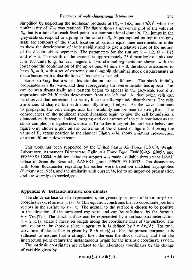
Dynamics of multi-dimensional detonation 265
simplified by neglecting the nonlinear products of (D, - l)b,, and (Obn)2, while the nonlinearity of ~ ? C J was retained. The figure shows a grey-scale plot of the value of D, that is attained at each fixed point in a computational domain. The jumps in the grey-scale correspond to a jump in the value of D,. Superimposed on top of the grey scale are contours of the shock location at various equal time increments, in order to show the development of the instability and to give a relative sense of the motion of the disjoint shock segments. The parameters for the run are y = 1.2, Q = 1.85 and E = 5. The width of the channel is approximately 25 dimensionless units and it is 100 units long, for each segment. Two channel segments are shown, with the lower one the continuation of the upper one. At time t = 0, the shock is assumed to have D, = 0, with a set of extremely small-amplitude initial shock displacements as disturbances with a distribution of frequencies excited.
The shock initially propagates as a flat wave, and then subsequently transverse instabilities appear. This can be seen dramatically as a pattern begins to appear in the grey-scale record at approximately 25-30 units downstream from the left end. At that point, cells can be observed that correspond to nearly linear small-amplitude disturbances. The cells are diamond shaped, but with nominally straight edges. As the wave continues to propagate, the cells merge, and the instability can be seen to strengthen. The consequences of the nonlinear shock dynamics begin to give the cell boundaries a diamond-spade shaped. Indeed, merging and coalescence of the cells continues as the shock complex propagates downstream. To further interpret the nonlinear behaviour, figure 6(a), shows a plot on the centreline of the channel of figure 5, showing the value of D, versus position in the channel. Figure 6(b), shows a similar cross-section at about 50 units downstream.
Some striking features of this simulation are as follows.
This work has been supported by the United States Air Force (USAF), Wright Laboratory, Armament Directorate, Eglin Air Force Base, F08630-92- K0057, and F08630-95- 10004. Additional student support was made available through the USAF Office of Scientific Research, AASERT grant F49620-93-1-0532. The discussions with John Buckmaster regarding his earlier work based on matched asymptotics (Buckmaster 1988), and the similarity with ours in 96, led to an improved presentation and are warmly acknowledged.
Appendix A. Betrand-intrinsic coordinates The shock surface can be represented quite generally in terms of laboratory-fixed
coordinates (x, y ) as y(x, y , t) = 0. This equation constrains the lab-coordinate position vectors in the surface to x = x,. The normal to the surface is chosen to be positive in the direction of the unreacted explosive and can be calculated by the formula 2 = Vw/lVyl. The shock surface can be represented by a surface parameterization x = x s ( t , t ) , where 5 measures length along the coordinate lines of the surface. The unit vector in the shock surface, tangent to it, is defined by ? = ax,/a<. The total curvature of the surface is given by V D = ~ ( 5 , t). For the present purpose, it is sufficient to assume that a straight line intersects the shock surface, and that the intersection point defines the instantaneous origin for the intrinsic coordinate system.
The intrinsic coordinates are related to the laboratory coordinates by the change of variable given by
(A 1) x = x,(<,t) + ni i ( t , t ) .

266 J. Yao and D. S. Stewart
1.20
Drl
1 .oo
0.0 25.0 50.0 75.0 100.0 125.0 150.0 175.0
(4
1.20
D”
1 .oo
0.0 10.0 20.0
FIGURE 6. (a) Solution of simplified (6.84) shown as a grey-scale contour plot of D,, for E = 5, Q = 1.85, y = 1.2. The simulated foil is shown in two piece and each is 25 wide and 100 units long. The foil records the value of D, as the shock passes by a fixed point. Lighter shades correspond to low values of D,, darker shades correspond to higher values, and D, ranges from approximately 0.9 to 1.3. Line contours show instantaneous shock positions at equal increments in time. (b) Longitudinal centre slice across the foils shown in (a) that shows plots D, versus position along the centre line. (b) Horizontal slice across the foils shown in (a) at approximately 75 units that shows plots D, versus vertical position along the cut.

Dynamics of multi-dimensional detonation
The Frenet formulas in two-dimensions are
A aii A
- --Kn, - = ICt. a? a< a< _ -
267
and reflect the fact the intrinsic coordinate system is locally orthogonal. Notice that in two-dimensions, one can define the angle 4 between a straight
reference line and the normal B. The derivative of the angle 4 with respect to the arclength 5 defines the curvature IC = a+/a<. Then normal and tangent unit vectors are related to the Cartesian basis by ii = sin(4)2, + cos(q5)2,, 2 = cos(4)2, - sin(+)2,. It is a straightforward matter to relate arclength, angle coordinates to laboratory coordinates.
The equations of motion are transformed from a representation in (x,y,t)- coordinates to (n, <, t)-coordinates according to coordinate transformation (A 1). The calculations required are straightforward but lengthy. Here we give the essential results needed. More details can be found in Lee, (1992), Stewart (1993) and Yao (1995). In what follows, with regard to fixed quantities in partial differentiation, x refers to (x ,y ) , and [ refers to (t,n).
The V operator is given by
By using the definition of the velocity in the intrinsic coordinates u = u$ + u,i, we calculate the divergence V u, and u - V as
The time derivative in the lab-fixed coordinates is related to that in the shock- attached coordinates by (a/&), = (a/&), + (anlat), (a/&) + (a</&), (d/at), where (an/at), = -D, is the negative of the normal component of the shock surface velocity and (a</&), = B , when evaluated at n = 0, is the instantaneous rate of increase or decrease of arclength along the shock. Thus we write
Next we derive the kinematic relations which gives a differential condition on B, in particular, which we later use to estimate the asymptotic order of certain terms in the transformed equations, for small curvature. Differentiating the change of variable formula (A 1) with respect to t, holding x fixed (and using the chain rule and Frenet formulas) gives,
Next we differentiate (A 6) with respect to 5 , holding n and t fixed, and use the Frenet formulas to obtain a vector equation, whose A- and ?-components are
aD, 1 , a t l+nlc '
268 J. Yao and D. S . Stewart
Equation (A7) can be further simplified. By differentiating (A7) by <, and by using the result that a/at[h-(a?/at)t] = -arc/at, one obtains an expression for &/at. Then using that formula in (A 8), one obtains the simple expression
In particular, (A9) can be used to estimate the size of B = ( d g / a t ) , . When specialized to the surface n = 0, the kinematic relations (A7) and (A9)
describe the evolution of the surface itself and reduce to the kinematic surface relations
Appendix B. Reduced governing equations The governing equations in Bertrand-intrinsic coordinates follow from a straight-
forward application of the formulas of Appendix A. If we define U,, = u, - D,, the governing equations are written as
where

Dynamics of multi-dimensional detonation 269
Notice that in equation (B2), that i>, = (aD,/dt), + BaD,/a( appears explicitly, which is the intrinsic time derivative of D, along the shock normal.
In addition, it is necessary to write down two independent energy equations, that can be used to replace the n-momentum and energy equations respectively; these are essentially a streamwise Bernoulli's equation and what has been called the muster equation, Bdzil (1981). Bernoulli's equation is given by
The master equation is written as
where R = - [ypRl- uR2 + ( y - 1)(& + qR5)]. Next we find the form of the reduced equations that for our needs must be valid
in the asymptotic sense in a region near the shock n < 0 with n - O(1), as the shock curvature K --+ 0. Specifically we consider the size of the terms that comprise R1-R5.
We assume that the dimensionless shock curvature is small. Let the order of magnitude of the curvature be measured by e2, where 0 < E B ~ . We also assume that the transverse spatial variation of the structure of the flow field behind the shock is weak, and is characterized by the scaled transverse variable
Therefore in the governing equations we assume that a / a g = d / a [ = O(E) . It follows from (A9), and from the estimates D, - O(1), K - O(e2), that one
obtains an estimate for B = (a{/&), - O(e). If one first supposes that ut - O(e) and ap/ag - o(e), then R3 is o(6). Equation (B3), with R3 = 0, is the O ( E ) equation for uy, which can be integrated on its characteristic. Combined with the shock boundary condition that uc = 0 at n = 0, one find that uc = 0 to O(e). Thus we are led to the finer estimate that ut - o(e).
The terms RI-Rs are o(e2) = o(K), if one makes the modest assumption that
which can be guaranteed, given the previous assumption on the explicit scaling for 5, for any expansion of the reaction-zone structure where the 0(1) terms are not functions of 4, and hence functions of at most n and t.
Note that no assumptions have been made so far regarding the asymptotic nature of the time variation, and its relation to the order of IC. However, if we further assume that we have slow-time variation in the shock-attached frame, and make only the assumption that ( d / a [ ) , - o(l), then the intrinsic derivative b, is approximated as (dDn/at)z + o ( ~ ) .

270 J. Yuo and D. S . Stewart
Appendix C. Limiting form of the steady (Dn, rc)-relation
limit as v + 1. Let Here we consider only the integral asymptotics of the result stated in $4, in the
i C J = 1 - ( Z * K ) I / V , (C 1)
(C 2) and D , be given by
D n - - 1 - ~ ( Z * X ) " ~ 2 - 1~7~1, where
where f' = (1 - 1)1/2. Note that in order to properly calculate the contribution to the integral I , when v + 1, one splits the integral from 0 to 1 into a contribution from 0 to 1 and 1 to AcJ. Hence for v < 1 one finds the second integral, and combines the result to obtain in the formula for D,:
D , , = ~ - K - di+- 2( 1 - v ) (z*rc)l/v + o(K'/v). (C 4) V
(Y + For the case that v = 1 we can also get a formula with a logarithmic contribution
that is identical the result in Stewart & Bdzil (1988), Klein & Stewart (1993). To demonstrate this, without loss of generality we take the rate multiplier to be equal to 1 and let c2(t') = y( 1 + t ) ( y - d)/(y + 1)2, and write the above result as
D, = 1-rc- (1 + /)2( 1 - A)-'(e'/'* - es/cz(o))dA (Y + y2 I'
1 --d KZ* ( (1+ / )2 - l ) ( l -A) -vdA-~ [*- 2 2 1 - v 1-v
Now we evaluate the last two terms: the term
1 2 4 - 2 ~ 3-2~'
1 ;i ((1+/)2-1)(1-i)-vdA= -+-
with v = 1, is equal to 5/2. We also rewrite
which can be evaluated with L'Hospital's rule as v --+ 1, and which generates a logarithm.
Finally we obtain
1' (1 + f')2(1 - 1)-v(e-e/c2 - e-'/'*('))dl + $z'rcln(z'rc).
(C 8) 1

Dynamics of multi-dimensional detonation 27 1
Appendix D. The integrals with the simplest rate law (zero activation energy)
First we calculate the integrals for D = 1 and r = (1 - A)" :
(L 2 y + l 1 - v + - ) ,
I1 = -
I 3 = ~ 1 (- 2Y - -) 1 ( y + 1 ) 2 3-2v 2-v '
2 14 = -
3 - 2 ~ ' Note that integral J does not contribute to G(D) when D = 1, because TCJ = 0.
integrals, with t = (1 - jZ/D2)ll2 : For the case that D is 1 to calculate those integrals we first define some simpler
~I
For I = (I - A)" = (1 - D2 + /2D2)v, we have
(D 7)
(D 8)
1 1 - v
K1 = -(1 - (1 - D2)'-"),
2 3 0
K2 = -( 1 - D2)3'2-vf'F[3/2, V, 5/2, D2/(D2 - l)],
1 K3 = -
0 2
1 - (1 - D2)2-" 1 - (1 - D2)'-" - (1 - D2) ( 2-v 1 - v
where F(a, b, c, z) is the hypergeometic function defined by the series
O0 r ( a + n)r(b + n) zn F(a, ~ , c , z ) = r(C) c - r ( a ) r ( b ) n=O r ( C + n ) n!'
Thus we obtain 1
11 = -(K1 + K2), Y + l
272 J . Yao and D. S . Stewart
I4 = K2
1
Y + l J = -(KO - yK1).
Appendix E. A list of integrals and relations
evolution equation in $6. Here we list several basic relations and integrals which are needed for deriving the
The definition of the constants C1 - C, In this section we define the constants referred to in the main text. One only needs to specify values for y and 6 and then follow the nested definitions to obtain the constants defined below.
First we define the following:
y-1+26 y + l '
v, =
1
V S Ps = - Y
y-11226 y + l '
us = -

Dynamics of multi-dimensional detonation 273
9 (E 12) 2 + S(1- l / y )
Y + l Ps =
(E 13a-d) Y + l 2
+
7 cs = Y P S V S , Y + J Y + 6
U l J = -- y + 1 ’ p > J = m , P > J = -
1 - 6 a= [3y-y2-S(3y-1)], p= ~ ‘)[2~-6(y-l)][y-1+26)~], (E 14a,b)
-
2(Y + ( Y +
= (y - 1 + 2S)2(3 + S) [ [Y - 3 + S(Y + 3 1 + (y + -
(E.16)
(E 17a, b)
(E 18a,b)
(E.19)
(E.20)
(E.21)
(E.22)
(E.23)
(E.25)
then
(23 = - 1 [ ( y + 6 ) 2 + y ( y + 6 ) ( 1 + U s ) + ( y 2 - 1 ) ( 1 + U s + ~ ~ ) ~ ~ + ~ (E.27) 1 - S 2 a 1 - 6 2 ’

274 J. Yao and D. S. Stewart 04
T3, L S
c4 = -p (1 - 62)a
- c," [3(y + 6) - 76 - 11 - 8 5 2 ( y + 1)(1+6) '
(E.28)
(E.29)
(E.30)
(E.31)
The limiting form of the evolution equation can be then expressed as
REFERENCES
ASLAM, T. D., BDZIL, J. B. & STEWART, D. S. 1995 Level-set techniques applied to modeling detonation shock dynamics. J. Comput. Phys. (submited). Also TAM Rep. 773, UIUC-ENG- 94-6029, University of Illinois, June 1995.
BDZIL, J. B. 1981 Steady state two-dimensional detonation. J. Fluid Mech. 108, 185-226. BDZIL, J. B. & STEWART, D. S. 1989 Modeling of two-dimensional detonation with detonation shock
BUCKMASTER, J. D. 1988 Pressure transients and the genesis of transverse shock in unstable
ERPENBECK, J. J. 1964 The stability of idealized one dimensional detonations. Phys. Fluids 7 ,
FICKETT, W. & WOOD, W. W. 1966 Flow calculations for pulsating one-dimensional detonations.
KLEIN, R., KROC, J. C. & SHEPHERD, J. E. 1995 Critical conditions for quasi-steady curved
KLEIN, R. & STEWART, D. S. 1993 The relation between curvature and rate state-dependent
LEE, H. I. & STEWART, D. S. 1990 Calculation of linear detonation instability: one-dimension
LEE, J. 1990 Detonation shock dynamics of composite energetic materials. PhD thesis, New Mexico
OSHER, S. & SETHIAN, J. 1988 Fronts propagating with curvature-dependent speed: Algorithms
dynamics. Phys. Fluids A 1, 1261-1267.
detonation. Combust. Sci. Tech. 61, 1-20.
6 8 M 9 6 .
Phys. Fluids 1, 528-534.
detonations. Reprint
detonation velocity. SIAM J. Appl. Maths 53, 1401-1435.
instability of plane detonation. J. Fluid Mech. 216, 103-132.
Institute of Mining and Technology, Soccoro, NM.
based on Hamiliton-Jacobi formulations. J . Comput. Phys. 79, 12-49

Dynamics of multi-dimensional detonation 275
STEWART, D. Scorn 1993 Lectures on detonation physics: Introduction to the theory of detonation shock dynamics. TAM Rep. 721. UILU-ENG-93-6019.
STEWART, D. S., ASLAM, T. D., YAO, J. & BDZIL, J. B. 1995 Level-set techniques applied to unsteady detonation propagation. Modeling in Combustion Science (ed. J. Buckmaster & T. Takeno). Lecture Notes in Physics, vol. 449, pp. 352-369. Springer. (Also TAM Rep. 773, UIUC-ENG- 94-6029, University of Illinois, Oct. 1994.)
STEWART, D. S. & BDZIL, J. B. 1988 The shock dynamics of stable multi-dimensional detonation. Combust. Flame 12, 311-323.
STEWART, D. S. & BDZIL, J. B. 1993 Asymptotics and multi-scale simulation in a numerical combustion laboratory. Asymptotic and Numerical Methods for Partial Diyerential Equations with Critical Parameters. NATO AS1 Series C: Vol 34, pp. 163-187.
STREHLOW, R. A., LIAUGMINAS, R., WATSON, R. H. & EYMAN, J. R. 1967 Transverse wave structures in detonation. Eleuenth Symp. ( int l ) on Combustion, pp. 683-691. Pittsburgh: The Combustion Institute.
WOOD, W. W. & KIRKWOOD, J. G. 1954 Diameter effects in condensed explosives: The relation between velocity and radius of curvature. J. Chem. Phys. 22, 1920-1924.
YAO, J. 1996 The dynamics of multi-dimensional detonation. PhD thesis, Theoretical and Applied Mechanics, University of Illinois.
YAO, J. & STEWART, D. S. 1995 On the normal detonation shock velocity curvature relationship for materials with large-activation energy. Combust. Flame 100, 5 19-528.