Noname manuscript No.(will be inserted by the editor)

Multi-Dimensional Top-k Dominating Queries

Man Lung Yiu · Nikos Mamoulis

Abstract The top-k dominating query returnsk data ob-jects which dominate the highest number of objects in adataset. This query is an important tool for decision supportsince it provides data analysts an intuitive way for findingsignificant objects. In addition, it combines the advantagesof top-k and skyline queries without sharing their disadvan-tages: (i) the output size can be controlled, (ii) no rankingfunctions need to be specified by users, and (iii) the resultis independent of the scales at different dimensions. De-spite their importance, top-k dominating queries have notreceived adequate attention from the research community.This paper is an extensive study on the evaluation of top-k dominating queries. First, we propose a set of algorithmsthat apply on indexed multi-dimensional data. Second, weinvestigate query evaluation on data that are not indexed. Fi-nally, we study a relaxed variant of the query which consid-ers dominance in dimensional subspaces. Experiments usingsynthetic and real datasets demonstrate that our algorithmssignificantly outperform a previous skyline-based approach.We also illustrate the applicability of this multi-dimensionalanalysis query by studying the meaningfulness of its resultson real data.

Keywords: Top-k Retrieval, Preference Dominance, ScoreCounting

1 Introduction

Consider a datasetD of points in ad-dimensional spaceRd.Given a (monotone) ranking functionF : Rd → R, a top-k

Man Lung YiuDepartment of Computer Science, Aalborg UniversityE-mail: mly@cs.aau.dk

Nikos MamoulisDepartment of Computer Science, University of Hong KongE-mail: nikos@cs.hku.hk

query[14,9] returnsk points with the smallestF value. Forexample, Figure 1a shows a set of hotels modeled by pointsin the 2D space, where the dimensions correspond to (pref-erence) attribute values; traveling time to a conference venueand room price. For the ranking functionF = x+y, the top-2 hotels arep4 andp6. An obvious advantage of the top-kquery is that the user is able to control the number of results(through the parameterk). On the other hand, it might notalways be easy for the user to specify an appropriate rank-ing function. In addition, there is no straightforward way fora data analyst to identify the most important objects usingtop-k queries, since different functions may infer differentrankings.

A skyline query[2] retrieves all points which are notdominated by any other point. Assuming that smaller valuesare preferable to larger at all dimensions, a pointp domi-natesanother pointp′ (i.e.,p � p′) when

(∃ i ∈ [1, d], p[i] < p′[i]) ∧ (∀ i ∈ [1, d], p[i] ≤ p′[i])

wherep[i] denotes the coordinate ofp in thei-th dimension.Continuing with the example in Figure 1a, the skyline queryreturns pointsp1, p4, p6, andp7. [2] showed that the skylinecontains the top-1 result for any monotone ranking function;therefore, it can be used by decision makers to identify po-tentially important objects to some database users. A keyadvantage of the skyline query is that it does not require theuse of a specific ranking function; its results only dependon the intrinsic characteristics of the data. Furthermore, theskyline is not affected by potentially different scales at dif-ferent dimensions (monetary unit or time unit in the exampleof Figure 1a); only the order of the dimensional projectionsof the objects is important. On the other hand, the size ofthe skyline cannot be controlled by the user and it can be aslarge as the data size in the worst case. As a result, the usermay be overwhelmed as she may have to examine numerousskyline points manually in order to identify the ones thatwill eventually be regarded as important. In fact, the skyline

2

may not be used as an informative and concise summaryfor the dataset. It is well known that [2]: for a fully corre-lated dataset, the skyline contains exactly 1 point, which isnot informative about the distribution of other data points;for a totally anti-correlated dataset, the skyline is the wholedataset, which is definitely not a concise data summary.

p

x (time to conf. venue)

0.5 1

0.5

1

y (price)

F=x+y

1 p2

p3

p4

p5

p6

p7

p

0.5 1

0.5

1

3

p1 p

2 p4

50 points

(a) dataset with 7 hotels (b) dataset with 54 hotels

Fig. 1 Features of hotels

To summarize, top-k queries do not provide an objectiveorder of importance for the points, because their results aresensitive to the preference function used. Skyline queries,on the other hand, only provide a subset of important points,which may have arbitrary size. To facilitate analysts, whomay be interested in a natural order of importance, accord-ing to dominance, we propose the following intuitive scorefunction:

τ(p) = | { p′ ∈ D | p � p′ } | (1)

In words, thescoreτ(p) is the number of points dominatedby pointp. The following monotone property holds forτ :

∀ p, p′ ∈ D, p � p′ ⇒ τ(p) > τ(p′) (2)

Based on theτ function, we can define a natural or-dering of the points in the database. Accordingly, thetop-k dominatingquery returnsk points inD with the highestscore. For example, the top-2 dominating query on the dataof Figure 1a retrievesp4 (with τ(p4) = 3) and p5 (withτ(p5) = 2). This result may indicate to a data analyst (i.e.,conference organizer) the most popular hotels to the con-ference participants (considering price and traveling time asselection factors). Here the popularity of a hotelp is definedbased on over how many other hotels wouldp be preferred,for any preference function.

As another example on how theτ function is relatedto popularity, consider a dataset with 54 hotels, as shownin Figure 1b. 50 of these points are not shown explicitly;the figure only illustrates a rectangle which includes all ofthem. The top-2 dominating points in this case arep1 (withτ(p1) = 51) andp2 (with τ(p2) = 50). Even thoughp2

is not a skyline point, it becomes important after the top-1hotelp1 has been fully booked. The reason is thatp2 is guar-anteed to be better than at least 50 points, regardless of any

monotone preference ranking function considered by indi-vidual conference participants. On the other hand, skylinepoint p3 may not provide such guarantee; in the worst case,all conference participants may just be looking for cheap ho-tels, sop3 is no good at all. A similar observation holds forthe skyline pointp4.

The above examples illustrate that a top-k dominatingquery is a powerful decision support tool, since it identi-fies the most significant objects in an intuitive way. Froma practical perspective, top-k dominating queries combinethe advantages of top-k queries and skyline queries withoutsharing their disadvantages. The number of results can becontrolled without specifying any ranking function. In addi-tion, data normalization is not required; the results are notaffected by different scales or data distributions at differentdimensions.

The top-k dominating query was first introduced by Pa-padias et al. [24] as an extension of the skyline query. How-ever, the importance and practicability of the query was notidentified there. This paper is an extensive study of this analy-sis query. We note that the R-tree (used in [24]) may not bethe most appropriate index for this query; since computingτ(p) is in fact anaggregatequery, we can replace the R-treeby anaggregate R-tree(aR-tree) [17,23]. In addition, we ob-serve that the skyline-based approach proposed in [24] mayperform many unnecessary score countings, since the sky-line could be much larger thank.

Motivated by these observations, our first contributionincludes two specialized and very efficient methods for eval-uating top-k dominating queries on a dataset indexed byan aR-tree. We propose (i) a batch counting technique forcomputing scores of multiple points simultaneously, (ii) acounting-guided search algorithm for processing top-k dom-inating queries, and (iii) a priority-based tree traversal al-gorithm that retrieves query results by examining each treenode at most once. We enhance the performance of (ii) withlightweight counting, which derives relatively tight upperbound scores for non-leaf tree entries at low I/O cost. Fur-thermore, to our surprise, the intuitivebest-firsttraversal or-der [13,24] turns out not to be the most efficient for (iii) be-cause of potential partial dominance relationships betweenvisited entries. Thus, we perform a careful analysis on (iii)and propose anovel, efficient tree traversal orderfor it. Ex-tensive experiments show that our methods significantly out-perform the skyline-based approach of [24].

The above algorithms have been published in the prelim-inary version of this paper [31], where we also propose top-kdominating query variants such asaggregatetop-k dominat-ing queries andbichromatictop-k dominating queries; theseextensions are not further investigated here. Instead, in thispaper, we examine two alternative topics relevant to top-kdominating queries. The first is the processing of top-k dom-inating queries on non-indexed data. In certain scenarios

3

(e.g., dynamically generated data), it is not always reason-able to assume an existing aR-tree index for them a priori. Inview of this, we propose a method that evaluates top-k dom-inating queries by accessing the (unordered) data only a fewtimes. As we demonstrate experimentally, this method sig-nificantly outperforms the best index-based method, whichrequires the bulk-loading an aR-tree index before evaluation.Our second extension over [31] is the proposal and study ofa relaxed form of the top-k dominating query. In this queryvariant, theτ(p) score is defined by the number of dimen-sional subspaces where pointp dominates another pointp′.As we demonstrate, this query derives more meaningful re-sults than the basic top-k dominating query.

The rest of the paper is organized as follows. Section 2reviews the related work. Section 3 discusses the propertiesof top-k dominating search and proposes optimizations forthe existing solution in [24]. We then propose eager/lazy ap-proaches for evaluating top-k dominating queries. Section4 presents an eager approach that guides the search by de-riving tight score bounds for encountered non-leaf tree en-tries immediately. Section 5 develops an alternative, lazy ap-proach that defers score computation of visited entries andgradually refines their score bounds when more tree nodesare accessed. Section 6 presents techniques for processingtop-k dominating queries on non-indexed data. Section 7 in-troduces the relaxed top-k dominating query and discussesits evaluation. In Section 8, experiments are conducted onboth real and synthetic datasets to demonstrate that the pro-posed algorithms are efficient and also top-k dominatingqueries return meaningful results to users. Section 9 sum-marizes our experimental findings and discusses the case ofhigh dimensional data. Finally, Section 10 concludes the pa-per.

2 Related Work

Top-k dominating queries include a counting component,i.e., multi-dimensional aggregation; thus, we review relatedwork on spatial aggregation processing. In addition, as thedominance relationship is relevant to skyline queries, wesurvey existing methods for computing skylines.

2.1 Spatial Aggregation Processing

R-trees [12] have been extensively used as access methodsfor multi-dimensional data and for processing spatial queries,e.g., range queries, nearest neighbors [13], and skylinequeries [24]. The aggregate R-tree (aR-tree) [17,23] aug-ments to each non-leaf entry of the R-tree an aggregate mea-sure of all data points in the subtree pointed by it. It has beenused to speed up the evaluation of spatial aggregate queries,

where measures (e.g., number of buildings) in a spatial re-gion (e.g., a district) are aggregated.

x0.5 1

0.5

1

y

e1 e

2

e3 e

4

e5

e6

e7

e13e

9

e10

e11

e12

e14

e15 e

16

e8

e17

e18

e19

e20

W

e1

e2

contents of leaf nodes omitted

10

e3

e4

e5

e6

e7

e8

e9

e10

e11

e12

e13

e14

e15

e16

e17

e18

e19

e20

10 10 10

2 3

3 2

3 2

2 3

3 2

2 3

2 3

3 2

root node

(a) a set of points (b) aCOUNTaR-tree

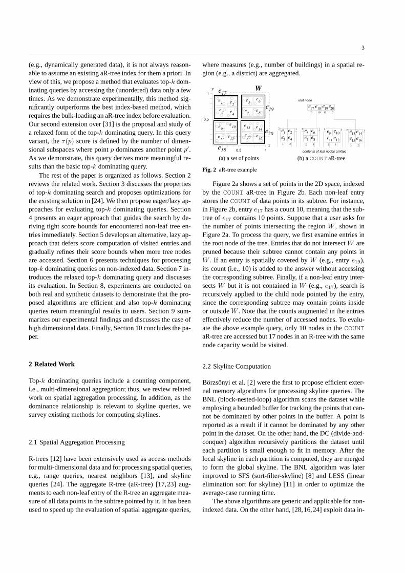
Fig. 2 aR-tree example

Figure 2a shows a set of points in the 2D space, indexedby the COUNTaR-tree in Figure 2b. Each non-leaf entrystores theCOUNTof data points in its subtree. For instance,in Figure 2b, entrye17 has a count 10, meaning that the sub-tree ofe17 contains 10 points. Suppose that a user asks forthe number of points intersecting the regionW , shown inFigure 2a. To process the query, we first examine entries inthe root node of the tree. Entries that do not intersectW arepruned because their subtree cannot contain any points inW . If an entry is spatially covered byW (e.g., entrye19),its count (i.e., 10) is added to the answer without accessingthe corresponding subtree. Finally, if a non-leaf entry inter-sectsW but it is not contained inW (e.g.,e17), search isrecursively applied to the child node pointed by the entry,since the corresponding subtree may contain points insideor outsideW . Note that the counts augmented in the entrieseffectively reduce the number of accessed nodes. To evalu-ate the above example query, only 10 nodes in theCOUNTaR-tree are accessed but 17 nodes in an R-tree with the samenode capacity would be visited.

2.2 Skyline Computation

Borzsonyi et al. [2] were the first to propose efficient exter-nal memory algorithms for processing skyline queries. TheBNL (block-nested-loop) algorithm scans the dataset whileemploying a bounded buffer for tracking the points that can-not be dominated by other points in the buffer. A point isreported as a result if it cannot be dominated by any otherpoint in the dataset. On the other hand, the DC (divide-and-conquer) algorithm recursively partitions the dataset untileach partition is small enough to fit in memory. After thelocal skyline in each partition is computed, they are mergedto form the global skyline. The BNL algorithm was laterimproved to SFS (sort-filter-skyline) [8] and LESS (linearelimination sort for skyline) [11] in order to optimize theaverage-case running time.

The above algorithms are generic and applicable for non-indexed data. On the other hand, [28,16,24] exploit data in-

4

dexes to accelerate skyline computation. The state-of-the-artalgorithm is the BBS (branch-and-bound skyline) algorithm[24], which is shown to be I/O optimal for computing sky-lines on datasets indexed by R-trees.

Recently, the research focus has been shifted to the studyof queries based on variants of the dominance relationship.[22] aims at extracting from the skyline points ak-sizedsubset such that it dominates the maximum number of datapoints; in other words, the result set cannot contain any non-skyline point. [20] proposes a data cube structure for speed-ing up the evaluation of queries that analyze the dominancerelationship of points in the dataset. However, incrementalmaintenance of the data cube over updates has not been ad-dressed in [20]. Clearly, it is prohibitively expensive to re-compute the data cube from scratch for dynamic datasetswith frequent updates. [6] identifies the problem of com-puting top-k frequent skylinepoints, where the frequencyof a point is defined by the number of dimensional sub-spaces. [5] studies thek-dominant skylinequery, which isbased on thek-dominance relationship. A pointp is saidto k-dominate another pointp′ if p dominatesp′ in at leastonek-dimensional subspace. Thek-dominant skyline con-tains the points that are notk-dominated by any other point.Whenk decreases, the size of thek-dominant skyline alsodecreases. Observe that [22,20,6,5] cannot be directly ap-plied to evaluate top-k dominating queries studied in thispaper.

Finally, [32,26,27,25] study the efficient computation ofskylines for every subspace; [29] proposes a technique forretrieving the skyline for a given subspace; [1,15] investi-gate skyline computation over distributed data; [10,7] de-velop techniques for estimating the skyline cardinality; [21]studies continuous maintenance of the skyline over a datastream; and [4] addresses skyline computation over datasetswith partially-ordered attributes.

3 Preliminary

In this section, we discuss some fundamental properties oftop-k dominating search, assuming that the data have beenindexed by an aR-tree. In addition, we propose an optimizedversion for the existing top-k dominating algorithm [24] thatoperates on aR-trees.

3.1 Score Bounding Functions

Before presenting our top-k dominating algorithms, we firstintroduce some notation that will be used in this paper. Foran aR-tree entrye (i.e., a minimum bounding box) whoseprojection on thei-th dimension is the interval[e[i]−, e[i]+],we denote its lower cornere− and upper cornere+ by

e− = (e[1]−, e[2]−, · · · , e[d]−)

e+ = (e[1]+, e[2]+, · · · , e[d]+)

Observe that bothe− and e+ do not correspond to actualdata points but they allow us to express dominance relation-ships among points and minimum bounding boxes conve-niently. As Figure 3 illustrates, there are three cases for apoint to dominate a non-leaf entry. Sincep1 � e−1 (i.e., fulldominance),p1 must also dominateall data points indexedundere1. On the other hand, pointp2 dominatese+1 but note−1 (i.e., partial dominance), thusp2 dominates some, butnot all data points ine1. Finally, asp3 � e+1 (i.e., no domi-nance),p3 cannot dominate any point ine1. Similarly, thecases for an entry to dominate another entry are: (i) fulldominance (e.g.,e+1 � e−3 ), (ii) partial dominance (e.g.,e−1 � e+4 ∧ e

+1 � e−4 ), (iii) no dominance (e.g.,e−1 � e+2 ).

+

_

p1

p3

p2

e1

e2

e3

e4

e5

e1

e1

Fig. 3 Dominance relationship among aR-tree entries

Given a tree entrye, whose sub-tree has not been visited,τ(e+) andτ(e−) correspond to thetightmostlower and up-per score bounds respectively, for any point indexed undere. As we will show later,τ(e+) andτ(e−) can be computedby a search procedure that accesses only aR-tree nodes thatintersecte along at least one dimension. These bounds helppruning the search space and defining a good order for vis-iting aR-tree nodes. Later in Sections 4 and 5, we replacethe tight boundsτ(e+) andτ(e−) with loose lower and up-per bounds for them (τ l(e) andτu(e), respectively). Boundsτ l(e) andτu(e) are cheaper to compute and can be progres-sively refined during search, therefore trading-off betweencomputation cost and bound tightness. The computation anduse of score bounds in practice will be further elaboratedthere.

3.2 Optimizing the Skyline-Based Approach

Papadias et al. [24] proposed a Skyline-Based Top-k Dom-inating Algorithm (STD) for top-k dominating queries, ondata indexed by an R-tree. They noted that the skyline isguaranteed to contain the top-1 dominating point, since anon-skyline point has lower score than at least one skylinepoint that dominates it (see Equation 2). Thus, STD retrievesthe skyline points, computes theirτ scores and outputs thepoint p with the highest score. It then removesp from the

5

dataset, incrementally finds the skyline of the remainingpoints, and repeats the same process.

Consider for example a top-2 dominating query on thedataset shown in Figure 4. STD first retrieves the skylinepointsp1, p2, andp3 (using the BBS skyline algorithm of[24]). For each skyline point, a range query is issued tocount the number of points it dominates. After that, we haveτ(p1) = 1, τ(p2) = 4, andτ(p3) = 1. Hence,p2 is reportedas the top-1 result. We now restrict the region of searchingfor the next result. First, Equation 2 suggests that the regiondominated by the remaining skyline points (i.e.,p1 andp3)needs not be examined. Second, the region dominated byp2 (i.e., the previous result) may contain some points whichare not dominated by the remaining skyline pointsp1 andp3. It suffices to retrieve the skyline points (i.e.,p4 andp5)in the constrained (gray) regionM shown in Figure 4. Af-ter counting their scores using the tree, we haveτ(p4) = 2andτ(p5) = 1. Finally, we compare them with the scoresof retrieved points (i.e.,p1 andp3) and reportp4 as the nextresult.

p

x (time to conf. venue)0.5 1

0.5

1

y (price)

F=x+y

1 p2

p3

p4

p5

p6 p7

x

0.5 1

0.5

1y

p2p3

p1 p6

p7

p4 p5

x0.5 1

0.5

1y

e1 e2e3 e4

e5e6

e7

e13e9e10

e11e12

e14e15 e16

e8

e17

e18

e19

e20

W

x

0.5 1

0.5

1y

p2p3

p1 p6

p7

p4 p5

M

e1 e2 e3

p1 p2 p3 p4 p5 p6 p7 p8 p9

e13 e14

e7 e8 e9

e1 e2 e3

e15

90 100 30

contents omitted

contents omitted

150 30 20

220 200 50

e16 e13 e14 e15e16 e13 e14 e15e16 e13 e14 e15e16

Fig. 4 Constrained skyline

In this section, we present two optimizations that greatlyreduce the I/O cost of the above solution by exploiting aR-trees. Our first optimization is calledbatch counting. Insteadof iteratively applying separate range queries to computethe scores of the skyline points, we perform them in batch.Algorithm 1 shows the pseudo-code of this recursive batchcounting procedure. It takes two parameters: the current aR-tree nodeZ and the set of pointsV , whoseτ scores are tobe counted. Initially,Z is set to the root node of the tree andτ(p) is set to 0 for eachp ∈ V . Let e be the current entryin Z to be examined. As illustrated in Section 3.1, ife is anon-leaf entry and there exists some pointp ∈ V such thatp � e+ ∧ p � e−, thenp may dominate some (but not guar-anteed to dominate all) points indexed undere. Thus, wecannot immediately decide the number of points ine dom-inated byp. In this case, we have to invoke the algorithmrecursively on the child node pointed bye. Otherwise, foreach pointp ∈ V , its score is incremented byCOUNT(e)when it dominatese−. BatchCount correctly computes theτ score for allp ∈ V , at a single tree traversal.

Algorithm 2 is a pseudo-code of the Iterative Top-k Dom-inating Algorithm (ITD), which optimizes the STD algo-

Algorithm 1 Batch Countingalgorithm BatchCount(NodeZ, Point setV )

1: for all entriese ∈ Z do2: if Z is non-leaf and∃p ∈ V, p � e+ ∧ p � e− then3: read the child nodeZ′ pointed bye;4: BatchCount(Z′, V );5: else6: for all pointsp ∈ V do7: if p � e− then8: τ(p):=τ(p)+COUNT(e);

rithm of [24]. Like STD, ITD computes the top-k dominat-ing points iteratively. In the first iteration, ITD computes inV ′ the skyline of the whole dataset, while in subsequent it-erations, the computation isconstrainedto a regionM . Mis the region dominated by the reported pointq in the pre-vious iteration, but not any point in the setV of retrievedpoints in past iterations. At each loop, Lines 6–8 computethe scores for the points inV ′ in batches ofB points each(B ≤ |V ′|). By default, the value ofB is set to the numberof points that can fit into a memory page. Our second opti-mization is that we sort the points inV ′ by a space-fillingcurve (Hilbert ordering) [3] before applying batch counting,in order to increase the compactness of the MBR of a batch.After merging the constrained skyline with the global one,the objectq with the highestτ score is reported as the nextdominating object, removed fromV and used to computethe constrained skyline at the next iteration. The algorithmterminates afterk objects have been reported.

For instance, in Figure 4,q corresponds to point(0, 0)andV = ∅ in the first loop, thusM corresponds to thewhole space and the whole skyline{p1, p2, p3} is stored inV ′, the points there are sorted and split in batches and theirτ scores are counted using the BatchCount algorithm. In thebeginning of the second loop,q = p2, V = {p1, p3}, andMis the gray region in the figure.V ′ now becomes{p4, p5}and the corresponding scores are batch-counted. The nextpoint is then reported (e.g.,p4) and the algorithm continuesas long as more results are required.

Algorithm 2 Iterative Top-k Dominating Algorithm (ITD)algorithm ITD(TreeR, Integerk)

1: V :=∅; q:=origin point;2: for i := 1 to k do3: M :=region dominated byq but by no point inV ;4: V ′:=skyline points inM ;5: sort the points inV ′ by Hilbert ordering;6: for all batchesVc of (B) points inV ′ do7: initialize all scores of points inVc to 0;8: BatchCount(R.root,Vc);9: V :=V ∪ V ′;

10: q:=the point with maximum score inV ;11: removeq from V ;12: report q as thei-th result;

6

4 Counting-Guided Search

The skyline-based solution becomes inefficient for datasetswith large skylines asτ scores of many points are computed.In addition, not all skyline points have largeτ scores. Moti-vated by these observations, we study algorithms that solvethe problem directly, without depending on skyline compu-tations. This section presents aneagerapproach for the eval-uation of top-k dominating queries, which traverses the aR-tree and computes tight upper score bounds for encounterednon-leaf tree entries immediately; these bounds determinethe visiting order for the tree nodes. We discuss the basic al-gorithm, develop optimizations for it, and investigate by ananalytical study the improvements of these optimizations.

4.1 The Basic Algorithm

Recall from Section 3.1 that the score of any pointp in-dexed under an entrye is upper-bounded byτ(e−). Basedon this observation, we can design a method that traversesaR-tree nodes in descending order of their (upper bound)scores. The rationale is that points with high scores can beretrieved early and accesses to aR-tree nodes that do not con-tribute to the result can be avoided.

Algorithm 3 shows the pseudo code of the SimpleCounting-Guided Algorithm (SCG), which directs search bycounting upper bound scores of examined non-leaf entries.A max-heapH is employed for organizing the entries to bevisited in descending order of their scores.W is a min-heapfor managing the top-k dominating points as the algorithmprogresses, whileγ is thek-th score inW (used for prun-ing). First, the upper bound scoresτ(e−) of the aR-tree rootentries are computed in batch (using the BatchCount algo-rithm) and these are inserted into the max-heapH. Whilethe scoreτ(e−) of H ’s top entrye is higher thanγ (imply-ing that points with scores higher thanγ may be indexedundere), the top entry is deheaped, and the nodeZ pointedby e is visited. If Z is a non-leaf node, its entries are en-heaped, after BatchCount is called to compute their upperscore bounds. IfZ is a leaf node, the scores of the pointsin it are computed in batch and the top-k setW (alsoγ) isupdated, if applicable.

As an example, consider the top-1 dominating query onthe set of points in Figure 5. There are 3 leaf nodes and theircorresponding entries in the root node aree1, e2, ande3.First, upper bound scores for the root entries (i.e.,τ(e−1 ) =3, τ(e−2 ) = 7, τ(e−3 ) = 3) are computed by the batch count-ing algorithm, which incurs 3 node accesses (i.e., the rootnode and leaf nodes pointed bye1 ande3). Sincee2 has thehighest upper bound score, the leaf node pointed bye2 willbe accessed next. Scores of entries ine2 are computed inbatch and we obtainτ(p1) = 5, τ(p2) = 1, τ(p3) = 2.Sincep1 is a point andτ(p1) is higher than the scores of

Algorithm 3 Simple Counting Guided Algorithm (SCG)algorithm SCG(TreeR, Integerk)

1: H:=new max-heap;W :=new min-heap;2: γ:=0; . thek-th highest score found so far3: BatchCount(R.root,{e− | e ∈ R.root});4: for all entriese ∈ R.root do5: enheap(H, 〈e, τ(e−)〉);6: while |H| > 0 andH ’s top entry’s score> γ do7: e:=deheap(H);8: read the child nodeZ pointed bye;9: if Z is non-leafthen

10: BatchCount(R.root,{e−c | ec ∈ Z});11: for all entriesec ∈ Z do12: enheap(H, 〈ec, τ(e

−c )〉);

13: else . Z is a leaf14: BatchCount(R.root,{p | p ∈ Z});15: updateW andγ, using〈p, τ(p)〉, ∀p ∈ Z16: report W as the result;

remaining entries (p2, p3, e1, e3), p1 is guaranteed to be thetop-1 result.

x0.5 1

0.5

1

y

e1

e2

e3

p4

p5

p6

p7 p

8

p9

p3

p2

p1

Fig. 5 Computing upper bound scores

4.2 Optimizations

Now, we discuss three optimizations that can greatly reducethe cost of the basic SCG. First, we utilize encountered datapoints to strengthen the pruning power of the algorithm.Next, we apply a lazy counting method that delays the count-ing for points, in order to form better groups for batch count-ing. Finally, we develop a lightweight technique for derivingupper score bounds of non-leaf entries at low cost.The pruner set.SCG visits nodes and counts the scores ofpoints and entries, based only on the condition that the up-per bound score of their parent entry is greater thanγ. How-ever, we observe that points which have been counted, buthave scores at mostγ can also be used to prune early otherentries or points, which are dominated by them.1 Thus, wemaintain a pruner setF , which contains points that (i) havebeen counted exactly (i.e., at Line 15), (ii) have scores atmostγ, and (iii) are not dominated by any other point inF .The third condition ensures that only minimal information

1 Suppose that a pointp satisfiesτ(p) ≤ γ. Applying Equation 2, ifa pointp′ is dominated byp, then we haveτ(p′) < γ.

7

is kept inF .2 We perform the following changes to SCG inorder to useF . First, after deheaping an entrye (Line 7), wecheck whether there exists a pointp ∈ F , such thatp � e−.If yes, thene is pruned and the algorithm goes back to Line6. Second, before applying BatchCount at Lines 10 and 14,we eliminate any entries or points that are dominated by apoint inF .Lazy counting. The performance of SCG is negatively af-fected by executions of BatchCount for a small number ofpoints. A batch may have few points if many points in aleaf node are pruned with the help ofF . In order to avoidthis problem, we employ alazy countingtechnique, whichworks as follows. When a leaf node is visited (Line 13), in-stead of directly performing batch counting for the pointsp,those that are not pruned byF are inserted into a setL, withtheir upper bound scoreτ(e−) from the parent entry. If, afteran insertion, the size ofL exceedsB (the size of a batch),then BatchCount is executed for the contents ofL, and allW , γ, F are updated. Just before reporting the final resultset (Line 16), batch counting is performed for potential re-sultsp ∈ L not dominated by any point inF and with upperbound score greater thanγ. We found that the combined ef-fect of the pruner set and lazy counting lead to 30% I/O costreduction of SCG, in practice.Lightweight upper bound computation. As mentioned inSection 3.1, the tight upper score boundτ(e−) can be re-placed by a looser, cheaper to compute, boundτu(e). Wepropose an optimized version of SCG, called LightweightCounting Guided Algorithm (LCG). Line 10 of SCG (Al-gorithm 3) is replaced by a call to LightBatchCount, whichis a variation of BatchCount. In specific, when bounds for asetV of non-leafentries are counted, the algorithm avoidsexpensive accesses at aR-tree leaf nodes, but uses entries atnon-leaf nodes to derive looser bounds.

LightBatchCount is identical to Algorithm 1, except thatthe recursion of Line 2 is applied whenZ is at least twolevels above leaf nodes and there is a point inV that partiallydominatese; thus, the else statement at Line 5 now refers tonodes one level above the leaves. In addition, the conditionat Line 7 is replaced byp � e+; i.e.,COUNT(e) is added toτu(p), even ifp partially dominates entrye.

As an example, consider the three root entries of Fig-ure 5. We can compute loose upper score bounds forV ={e−1 , e

−2 , e

−3 }, without accessing the leaf nodes. Since,e−2

fully dominatese2 and partially dominatese1, e3, we getτu(e2) = 9. Similarly, we getτu(e1) = 3 andτu(e3) = 3.Although these bounds are looser than the respective tightones, they still provide a good order of visiting the entriesand they can be used for pruning and checking for termi-nation. In Section 8, we demonstrate the significant compu-tation savings by this lightweight counting (ofτu(e)) overexact counting (ofτ(e−)) and show that it affects very little

2 Note thatF is the skyline of a specific data subset.

the pruning power of the algorithm. Next, we investigate itseffectiveness by a theoretical analysis.

4.3 Analytical Study

Consider a datasetD with N points, indexed by an aR-treewhose nodes have an average fanoutf . Our analysis is basedon the assumption that the data points are uniformly and in-dependently distributed in the domain space[0, 1]d, wheredis the dimensionality. Then, the tree heighth and the numberof nodesni at leveli (let the leaf level be0) can be estimatedby h = 1 + dlogf (N/f)e andni = N/f i+1. Besides, theextent (i.e., length of any 1D projection)λi of a node at thei-th level can be approximated byλi = (1/ni)1/d [30].

We now discuss the trade-off of lightweight countingover exact counting for a non-leaf entrye. Recall that theexactupper bound scoreτ(e−) is counted as the numberof points dominated by its lower cornere−. On the otherhand, lightweight counting obtainsτu(e); an upper boundof τ(e−). For a givene−, Figure 6 shows that the spacecan be divided into three regions, with respect to nodes atlevel i. The gray regionM2 corresponds to the maximalregion, covering nodes (at leveli) that arepartially domi-nated bye−. While computingτ(e−), only the entries whicharecompletely insideM2 need to be further examined (e.g.,eA). Other entries are pruned after either disregarding theiraggregate values (e.g.,eB , which intersectsM1), or addingthese values toτ(e−) (e.g.,eC , which intersectsM3).

+

_

p1

p3

p2

e1

e2e3

e4

e5

e1

e1

e

_M1 M2

M3λ i λ i

λ i

λ i

e_M1M2

M3

λ i λ i

λ i

λ i

(0,0)

(0,1)

(1,0)

(1,1)

eA

eB

eC

Fig. 6 I/O cost of computing upper bound

Thus, the probability of accessing a (i-th level) node canbe approximated by the area ofM2, assuming that tree nodesat the same level have no overlapping. To further simplifyour analysis, suppose that all coordinates ofe− are of thesame valuev. Hence, the aR-tree node accesses required forcomputing the exactτ(e−) can be expressed as3:

NAexact(e−) =h−1∑i=0

ni · [(1−v+λi)d− (1−v−λi)d] (3)

3 For simplicity, the equation does not consider the boundary effect(i.e., v is near the domain boundary). To capture the boundary effect,we need to bound the terms(1 − v + λi) and(1 − v − λi) within therange[0, 1].

8

In the above equation, the quantity in the square bracketscorresponds to the volume ofM2 (at level i) over the vol-ume of the universe (this equals to 1), capturing thus theprobability of a node at leveli to be completely insideM2.The node accesses of lightweight computation can also becaptured by the above equation, except that no leaf nodes(i.e., at level 0) are accessed. As there are many more leafnodes than non-leaf nodes, lightweight computation incurssignificantly lower cost than exact computation.

Now, we compare the scores obtained by exact compu-tation and lightweight computation. The exact scoreτ(e−)is determined by the area dominated bye−:

τ(e−) = N · (1− v)d (4)

In addition to the above points, lightweight computation countsalso all points inM2 for the leaf level into the upper boundscore:

τu(e) = N · (1− v + λ0)d (5)

Summarizing, three factorsN , v, andd affect the rela-tive tightness of the lightweight score bound over the exactbound.

– WhenN is large, the leaf node extentλ0 is small andthus the lightweight score is tight.

– If v is small, i.e.,e− is close to the origin and has highdominating power, thenλ0 becomes less significant inEquation 5 and the ratio ofτu(e) to τ(e−) is close to 1(i.e., lightweight score becomes relatively tight).

– As d increases (decreases),λ0 also increases (decreases)and the lightweight score gets looser (tighter).

In practice, during counting-guided search, entries closeto the origin have higher probability to be accessed thanother entries, since their parent entries have higher upperbounds and they are prioritized by search. As a result, weexpect that the second case above will hold for most of theupper bound computations and lightweight computation willbe effective.

5 Priority-Based Traversal

In this section, we present alazyalternative to the counting-guided method. Instead of computing upper bounds of vis-ited entries by explicit counting, we defer score computa-tions for entries, but maintain lower and upper bounds forthem as the tree is traversed. Score bounds for visited en-tries are gradually refined when more nodes are accessed,until the result is finalized with the help of them. For thismethod to be effective, the tree is traversed with a carefully-designed priority order aiming at minimizing I/O cost. Wepresent the basic algorithm, analyze the issue of setting anappropriate order for visiting nodes, and discuss its imple-mentation.

5.1 The Basic Algorithm

Recall that counting-guided search, presented in the previ-ous section, may access some aR-tree nodes more than oncedue to the application of counting operations for the visitedentries. For instance in Figure 5, the node pointed bye1 maybe accessed twice; once for counting the scores of points un-dere2 and once for counting the scores of points undere1.We now propose a top-k dominating algorithm which tra-verses each node at most once and has reduced I/O cost.

Algorithm 4 shows the pseudo-code of this Priority-BasedTree Traversal Algorithm (PBT). PBT browses the tree, whilemaintaining (loose) upperτu(e) and lower τ l(e) scorebounds for the entriese that have been seen so far. The nodesof the tree are visited based on apriority order. The issue ofdefining an appropriate ordering of node visits will be elabo-rated later. During traversal, PBT maintains a setS of visitedaR-tree entries. An entry inS can either: (i) lead to a poten-tial result, or (ii) be partially dominated by other entries inSthat may end up in the result.W is a min-heap, employed fortracking the top-k points (in terms of theirτ l scores) foundso far, whereasγ is the lowest score inW (used for pruning).

First, the root node is loaded, and its entries are insertedinto S after upper score bounds have been derived from in-formation in the root node. Then (Lines 8-18), whileS con-tains non-leaf entries, the non-leaf entryez with the highestpriority is removed fromS, the corresponding tree nodeZis visited and (i) theτu (τ l) scores of existing entries inS(partially dominatingez) are refined using the contents ofZ,(ii) τu (τ l) values for the contents ofZ are computed and, inturn, inserted toS. Note that for operations (i) and (ii), onlyinformation from the current node andS is used; no addi-tional accesses to the tree are required. Updates and com-putations ofτu scores are performed incrementally with theinformation ofez and entries inS that partially dominateez.W is updated with points/entries of higherτ l thanγ. Finally(Line 20), entries are pruned fromS if (i) they cannot lead topoints that may be included inW , and (ii) are not partiallydominated by entries leading to points that can reachW .

It is important to note that, at Line 21 of PBT, all non-leaf entries have been removed from the setS, and thus (re-sult) points inW have their exact scores found.

To comprehend the functionality of PBT consider againthe top-1 dominating query on the example of Figure 5. Forthe ease of discussion, we denote the score bounds of an en-try e by the intervalτ?(e)=[τ l(e), τu(e)]. Initially, PBT ac-cesses the root node and its entries are inserted intoS aftertheir lower/upper bound scores are derived (see Lines 5–6);τ?(e1)=[0, 3], τ?(e2)=[0, 9], τ?(e3)=[0, 3]. Assume for now,that visited nodes are prioritized (Lines 9-10) based on theupper bound scoresτu(e) of entriese ∈ S. Entrye2, of thehighest scoreτu in S is removed and its child nodeZ isaccessed. Sincee−1 � e+2 ande−3 � e+2 , the upper/lower

9

Algorithm 4 Priority-Based Tree Traversal Algorithm(PBT)

algorithm PBT(TreeR, Integerk)1: S:=new set; . entry format inS: 〈e, τ l(e), τu(e)〉2: W :=new min-heap; . k points with the highestτ l

3: γ:=0; . thek-th highestτ l score found so far4: for all ex ∈ R.root do5: τ l(ex):=

Pe∈R.root∧e+

x �e−COUNT(e);

6: τu(ex):=P

e∈R.root∧e−x �e+COUNT(e);7: insertex into S and updateW ;8: while S contains non-leaf entriesdo9: removeez : non-leaf entry ofS with the highestpriority;

10: read the child nodeZ pointed byez ;11: for all ey ∈ S such thate+y � e−z ∧ e−y � e+z do12: τ l(ey):=τ l(ey) +

Pe∈Z∧e+

y �e−COUNT(e);

13: τu(ey):=τ l(ey) +P

e∈Z∧e+y �e−∧e−y �e+COUNT(e);

14: Sz :=Z ∪ {e ∈ S | e+z � e− ∧ e−z � e+};15: for all ex ∈ Z do16: τ l(ex):=τ l(ez) +

Pe∈Sz∧e+

x �e−COUNT(e);

17: τu(ex):=τ l(ex) +P

e∈Sz∧e+x �e−∧e−x �e+COUNT(e);

18: insert all entries ofZ into S;19: updateW (andγ) by e′ ∈ S whose score bounds changed;20: remove entriesem from S whereτu(em) < γ and¬∃e ∈

S, (τu(e) ≥ γ) ∧ (e+ � e−m ∧ e− � e+m);

21: report W as the result;

score bounds of remaining entries{e1, e3} in S will not beupdated (the condition of Line 11 is not satisfied). The scorebounds for the pointsp1, p2, andp3 in Z are then computed;τ?(p1)=[1, 7], τ?(p2)=[0, 3], andτ?(p3)=[0, 3]. These pointsare inserted into S, and W={p1} withγ=τ l(p1)=1. No entry or point inS can be pruned, sincetheir upper bounds are all greater thanγ. The next non-leaf entry to be removed fromS is e1 (the tie with e3 isbroken arbitrarily). The score bounds of the existing entriesS={e3, p1, p2, p3} are in turn refined;τ?(e3) remains[0, 3](unaffected bye1), whereasτ?(p1)=[3, 6], τ?(p2)=[1, 1], andτ?(p3) =[0, 3]. The scores of the points indexed bye1 arecomputed;τ?(p4)=[0, 0], τ?(p5)=[0, 0], andτ?(p6)=[1, 1] andW is updated top1 with γ=τ l(p1)=3. At this stage, all points,except fromp1, are pruned fromS, since theirτu scores areat mostγ and they are not partially dominated by non-leafentries that may contain potential results. Although no pointfrom e3 can have higher score thanp1, we still have to keepe3, in order to compute the exact score ofp1 in the nextround.

5.2 Traversal Orders in PBT

An intuitive method for prioritizing entries at Line 9 of PBT,hinted by theupper bound principleof [19] or thebest-firstordering of [13,24], is to pick the entryez with the high-est upper bound scoreτu(ez); such an order would visit thepoints that have high probability to be in the top-k dominat-

ing result early. We denote this instantiation of PBT by UBT(for Upper-bound Based Traversal).

Nevertheless a closer look into PBT (Algorithm 4) re-veals that the upper score bounds alone may not offer thebest priority order for traversing the tree. Recall that thepruning operation (at Line 20) eliminates entries fromS,saving significant I/O cost and leading to the early termina-tion of the algorithm. The effectiveness of this pruning de-pends on thelower bounds of the best points (stored inW ).Unless these bounds are tight enough, PBT will not termi-nate early andS will grow very large.

For example, consider the application of UBT to the treeof Figure 2. The first few nodes accessed are in the order:root node,e18, e11, e9, e12. Although e11 has the highestupper bound score, itpartially dominateshigh-level entries(e.g., e17 and e20), whose child nodes have not been ac-cessed yet. As a result, the best-k scoreγ (i.e., the cur-rent lower bound score ofe11) is small, few entries can bepruned, and the algorithm does not terminate early.

Thus, the objective of search is not only to (i) examinethe entries of large upper bounds early, which leads to earlyidentification of candidate query results, but also (ii) elim-inate partial dominance relationships between entries thatappear inS, which facilitates the computation of tight lowerbounds for these candidates. We now investigate the factorsaffecting the probability that one node partially dominatesanother and link them to the traversal order of PBT. Letaand b be two random nodes of the tree such thata is atlevel i and b is at levelj. Using the same uniformity as-sumptions and notation as in Section 4.3, we can infer thatthe two nodesa andb not intersect along dimensiont withprobability4:

Pr(a[t] ∩ b[t] = ∅) = 1− (λi + λj)

a andb have a partial dominance relationship when they in-tersect along at least one dimension. The probability of be-ing such is:

Pr(∨

t∈[1,d]

a[t] ∩ b[t] 6= ∅) = 1− (1− (λi + λj))d

The above probability is small when the sumλi +λj is min-imized (e.g.,a andb are both at low levels).

The above analysis leads to the conclusion that in orderto minimize the partially dominating entry pairs inS, weshould prioritize the visited nodes based on their level at thetree. In addition, between entries at the highest level inS,we should choose the one with the highest upper bound, inorder to find the points with high scores early. Accordingly,we propose an instantiation of PBT, called Cost-Based Tra-versal (CBT). CBT corresponds to Algorithm 4, such that,

4 The current equation is simplified for readability. The probabilityequals 0 whenλi + λj > 1.

10

at Line 9, the non-leaf entryez with the highest level is re-moved fromS and processed; if there are ties, the entry withthe highest upper bound score is picked. In Section 8, wedemonstrate the advantage of CBT over UBT in practice.

5.3 Implementation Details

A straightforward implementation of PBT may lead to veryhigh computational cost. At each loop, the burden of the al-gorithm is the pruning step (Line 20 of Algorithm 4), whichhas worst-case cost quadratic to the size ofS; entries arepruned fromS if (i) their upper bound scores are belowγand (ii) they are not partially dominated by any other entrywith upper bound score aboveγ. If an entryem satisfies (i),then a scan ofS is required to check (ii).

In order to check for condition (ii) efficiently, we use amain-memory R-treeI(S) to index the entries inS havingupper bound score aboveγ. When the upper bound scoreof an entry drops belowγ, it is removed fromI(S). Whenchecking for pruning ofem at Line 20 of PBT, we only needto examine the entries indexed byI(S), as only these haveupper bound scores aboveγ. In particular, we may not evenhave to traverse the whole indexI(S). For instance, if anon-leaf entrye′ in I(S) does not partially dominateem,then we need not check for the subtree ofe′. As we verifiedexperimentally, maintainingI(S) enables the pruning stepto be implemented efficiently. In addition toI(S), we triedadditional data structures for accelerating the operations ofPBT (e.g., a priority queue for popping the next entry fromS at Line 9), however, the maintenance cost of these datastructures (as the upper bounds of entries inS change fre-quently at Lines 11-13) did not justify the performance gainsby them.

6 Query Processing on Non-indexed Data

This section examines the evaluation of top-k dominatingqueries on non-indexed data, assuming that data points arestored in random order in a disk fileD.

As discussed in [31], a practically viable solution is tofirst bulk-load an aR-tree (e.g., using the algorithm of [18])from the dataset and then compute top-k dominating pointsusing the algorithms proposed in Sections 4 and 5. The bulk-loading step requires externally sorting the points, which isknown to scale well for large datasets. However, externalsorting may incur multiple I/O passes over data.

Our goal is to compute the top-k dominating points withonly a constant number (3) of data passes, by adopting thefilter-refinement framework. The first pass is thecountingpass, which employs a memory grid structure to keep trackof point count in cells, while scanning over the data. Thisstructure is then used to derive lower/upper bound scores of

points in the next pass. The second pass is thefilter pass,which applies pruning rules to discard unqualified pointsand keep the remaining ones in a candidate set. Therefine-ment pass, being the final pass, performs a scan over the datain order to count the exactτ scores of all candidate points.Eventually, the top-k dominating points are returned.

In Section 6.1, we present the details of the countingpass. We investigate different techniques for the filter passin Sections 6.2 and 6.3; these techniques trade-off efficiency(i.e., CPU time at the filter step) for filter effectiveness (i.e.,size of the candidate set). Finally, Section 6.4 discusses thefinal, refinement pass of the algorithm.

6.1 The counting pass

The first step of the algorithm defines a regularmulti-dimensional grid over the space and performs a lin-ear scan to the data to count the number of points in eachgrid cell. Such a 2-dimensional histogram (with4× 4 cells)is shown in Figure 7a. To ease our discussion, each grid cellis labeled asgij . While scanning the points, we increase thecounters of the cells that contain them, but do not keep thevisited points in memory. In this example, at the end of scan,we haveCOUNT(g11)=0 andCOUNT(g12)=10. We adopt thefollowing convention so that each point contributes to thecounter of exactly one cell. In case a point (e.g.,p1) falls onthe common border of multiple cells (e.g.,g23 andg33), itbelongs to the cell (e.g.,g33) with the largest coordinates.

x

y

p1

p2

10g

14g

24

g13

g12

g11

g23

g22

g21

g34

g33

g32

g31

g44

g43

g42

g41

p3

10

10

10

10 10

0 10

10

10

10

10

10

10

10

10

x

y

: 40µ u: 30µ u

: 20µ u: 10µ u

: 80µ u: 60µ u

: 40µ u: 20µ u

: 120µ u: 90µ u

: 60µ u: 30µ u

: 150µ u: 120µ u

: 80µ u: 40µ u

φ : 10

φ : 20 φ : 50

φ : 30

φ : 80

φ : 50

φ : 20φ : 10

(a) Point counts of cells (b) Derived values of cells

x

y

p7

g24

g12

g23

g22

g21

g32

g42

p5

p4

p6

x

y

p11

g31

p14

p17

p23

p26

p29

(c) Tightening of score bounds (d) Points in the same cell

Fig. 7 Using the grid in the filter step,k=2

11

After the counting pass, and before the filter pass begins,we can derive lower/upper bound scores of the cells fromtheir point counts, by using the notations of Section 3.1. Thisenables us to determine fast the cells that cannot contain top-k dominating points. Given a grid cellg, its upper boundscoreτu(g) is the total point count of cells it partially ortotally dominates.

τu(g) =∑

gy∈G∧g−�g+y

COUNT(gy)

In Figure 7b, the cellg33 dominatesg33, g43, g34, andg44,so we haveτu(g33)=40. The lower bound scoreτ l(g) of gis the total point count of cells itfully dominates.

τ l(g) =∑

gy∈G∧g+�g−y

COUNT(gy)

For instance,g33 fully dominatesg44 so we obtainτ l(g33)=10(not shown in the figure).

Besides score bounds, pruning can also be achieved withthe help of the dominance property. From Equation 2, weobserve that, a point cannot belong to the result if it is domi-nated byk other points. Thus, we define the dominated countg.φ of the cellg as the total point count of cells fully domi-natingg.

g.φ =∑

gy∈G∧g+y �g−

COUNT(gy)

For example,g32 is fully dominated byg11 andg21, so weget g32.φ=0+10=10. Clearly, a cell withgij .φ ≥ k cannotcontain any of the top-k results.

Let k = 2 in the example of Figure 7b. We proceed todetermine the cells that cannot contain query results. Theseinclude cells with zero count (e.g.,g11) and cells havinggij .φ ≥ k (e.g.,g23). In order to obtain the valueγ (lowerbound score of top-k points), we enumerate the remainingcell(s) in descending order of theirτ l scores, until their totalpoint count reachesk. Since the cellg12 contains 10 (≥ k)points and itsτ l score is 60, we setγ = 60. Obviously,cells (e.g.,g14) whose upper score bounds belowγ = 60can be pruned. The remaining cells (containing potential re-sults) are colored as gray in Figure 7b.

6.2 Coarse-grained Filter

During, the second (filter) pass, the algorithm scans the dataagain and determines a set of candidate points for the top-k dominating query. The first method we propose for thefilter pass is calledcoarse-grained filter(CRS). CRS scansthe database and uses the score bounds of grid cells and thedominance property (of Equation 2) to prune points. CRSis described by Algorithm 5. Each cellg is coupled with acandidate setg.C, for maintaining candidate points that fall

in g (this is done only for cellsg that are not pruned afterthe counting pass). Initially, we have no information aboutthe detailed contents of the cells. However, using the lowerscore boundsτ l of the cells and their cardinalities, we caninitializeγ; thek-th highestτ l score of the top-k dominatingcandidates. In other words, we assume that each candidatehas the maximum coordinates in its container cellg (worstcase) and useτ l(g) as its lower bound. The algorithm thenperforms a linear scan over the datasetD at Lines 4–16. Forthe pointp being currently examined, we initialize its upperboundτu(p) anddominated countp.φ using the correspond-ing values of its container cellgp.

Algorithm 5 Coarse-grained Filter Algorithm (CRS-Filter)algorithm CRS-Filter(DatasetD, Integerk, GridG)

1: for all cell g ∈ G do2: g.C:=new set; . candidate set of the cell3: γ:=thek-th highestτ l score of cells inG; . for each cellg ∈ G,

COUNT(g) instances of the scoreτ l(g) are considered4: for all p ∈ D do . filter scan5: letgp be the grid cell ofp;6: τu(p):=τu(gp); p.φ:=gp.φ;7: for all cellsgz ∈ G such thatg−z � g+p ∧ g+z � g−p do8: for all p′ ∈ gz .C such thatp′ � p do9: p.φ:=p.φ+ 1;

10: if p.φ ≥ k then11: ignore further processing for the pointp;12: for all cellsgz ∈ G such thatg−p � g+z ∧ g+p � g−z do13: for all p′ ∈ gz .C such thatp � p′ do14: p′.φ:=p′.φ+ 1;15: if p′.φ ≥ k then16: removep′ from gz .C;17: if τu(p) ≥ γ andp.φ < k then18: insertp into gp.C;

In the loop of Lines 7–11, we search for candidate pointsp′ that dominatep and have already been read in memory.For each such occurrence, the valuep.φ is incremented. Dueto the presence of the dominated countgp.φ of the grid cell,it suffices to traverse only the cells that partially dominatethe cell ofp (as opposed to all cells). Wheneverp.φ reachesk, p.φ needs not be incremented further (and the loop exits);in this casep cannot be a top-k dominating result.

In the loop of Lines 12–16, we search for candidate pointsp′ that are dominated byp and have already been read inmemory. Thep′.φ of each such pointp′ is incremented; andthe point is pruned from the candidate set whenp′.φ reachesk. Note that Lines 12–16 need not be executed whenp.φis (at least)k. The reason is that any existing candidatep′

which is dominated byp must have also been dominated bythek dominators ofp and therefore already been pruned ina previous iteration.

At Lines 15–16, we insert the current pointp into thecandidate setgp.C of its cell gp, only when itsτu(p) scoreis aboveγ and itsp.φ value is less thank.

12

6.3 Fine-grained Filter

CRS simply sets the score bounds of candidate points tothose of their cells. Since each cell may contain a large num-ber of points, their score bounds are not tight, weakeningthe filter effectiveness of CRS. In this section, we developa fine-grained solution (FN) that tightens the score boundsof candidate points gradually. This way, more unqualifiedpoints having low scores can be eliminated from the searchearly.Tightening the score bounds of points.Consider the filterstep during the processing of the top-2 dominating query(i.e.,k=2) on Figure 7c. Suppose that, the pointsp4, p5, p6

are existing candidates (they have already been read duringthe filter pass), and the next point to be processed isp7.

The first technique is to tighten score bounds by usingthe current pointp7 and existing candidate pointsp4, p5, p6.First of all, we setτ l(p7) = 40 andτu(p7) = 90, by us-ing score bounds ofp7’s cell g22. To tighten score boundsof existing candidates, we traverse the cells (i.e.,g12, g22,g21) that partially dominateg22. Sincep4 dominatesp7, weincrementτ l(p4). On the other hand,p5 andp6 do not dom-inatep7 so theirτu scores are decremented. To tighten scorebounds of the current pointp7, we traverse the cells (e.g.,g22, g32, g42, g23, g24) that are partially dominated byg22.As p7 dominatesp6, we incrementτ l(p7). In addition, thedominated count ofp6 now becomes 2 (≥ k) so it is re-moved from the local candidate setg22.C.

A second technique that our filter algorithm uses to tightenscore bounds is by utilizing bounds of candidate points thathave not already been pruned. Assume in Figure 7d that, thepoint p17 is visited after pointsp11 and p14 (intermediatepoints likep12 have been pruned). In this case,τ l(p17) canbe tightened tomax{τ l(p17), τ l(p11), τ l(p14)}. As anotherexample, suppose that the pointp29 is visited after pointsp23

andp26. Then, the upper bound score ofp29 can be tightenedto min{τu(p29), τu(p23), τu(p26)}.Writing disk partitions. We observe that the pruning effec-tiveness of the algorithm can be significantly improved if weare able to identify points with high scores early. To achievethis, we modify the counting pass (described in Section 6.1)as follows. Each grid cellg is allocated a memory partition(at least one page) to store the accessed points that fall in thecell. Whenever the memory becomes full, the largest mem-ory partition is flushed into its corresponding disk partitiong.D (i.e., a sequential file). At the end of the counting pass,remaining points in memory are flushed into their respectivedisk partitions. This modification costs an additional writingpass over the data, yet it permits us to access the disk parti-tions using different orderings (in the subsequent filter andrefinement passes).Algorithm. Algorithm 6 presents the details of our Fine-grained Filter Algorithm (FN-Filter). A min-heapW is used

to keep track ofk points with the highestτ l scores seen sofar andγ is set to thek-th score inW . Like in the CRS-Filter, we first determine thek-th highest lower bound scoreγ from theτ l scores and point counts of grid cells. Then,kdummy pairs having the scoreγ are inserted intoW . ThesetS contains the grid cells whose disk partitions have yetto be visited. Initially, all grid cells are inserted intoS.

Algorithm 6 Fine-grained Filter Algorithm (FN-Filter)algorithm FN-Filter(DatasetD, Integerk, GridG)

1: γ:=thek-th highestτ l score of cells inG; . for each cellg ∈ G,COUNT(g) instances of the scoreτ l(g) are considered

2: W :=new min-heap; . k points with the highestτ l

3: insertk dummy pairs〈NULL, γ〉 intoW ;4: S:=new set; . set of grid cells5: for all cell g ∈ G do6: g.C:=new set; . candidate set of the cell7: letg.D be the disk partition ofg;8: insertg into S;9: while S is non-emptydo

10: removeg: the cell inS with the highestpriority;11: if τu(g) < γ and¬∃gz ∈ G, (τu(gz) ≥ γ) ∧ (g+z �

g− ∧ g−z � g+) then12: ignore further processing for the disk partitiong.D;13: for all p ∈ g.D do . scan over points in disk partitiong.D14: τ l(p):=τ l(g); τu(p):=τu(g); p.φ:=g.φ;15: δ.l:=−1; δ.u:=|D|; δ.φ:=−1;16: for all cell gz ∈ G such thatg−z � g+ ∧ g+z � g− do17: for all p′ ∈ gz .C do . existing candidates in memory18: if p′ � p then19: τ l(p′):=τ l(p′) + 1; p.φ:=p.φ+ 1;20: δ.u:=min{ δ.u, τu(p′) };21: δ.φ:=max{ δ.φ, p′.φ };22: else23: τu(p′):=τu(p′)− 1;

24: for all cell gz ∈ G such thatg− � g+z ∧ g+ � g−z do25: for all p′ ∈ gz .C do . existing candidates in memory26: if p � p′ then27: τ l(p):=τ l(p) + 1; p′.φ:=p′.φ+ 1;28: δ.l:=max{ δ.l, τ l(p′) };29: else30: τu(p):=τu(p)− 1;

31: τ l(p):=max{ τ l(p), δ.l }; τu(p):=min{ τu(p), δ.u };32: p.φ:=max{ p.φ, δ.φ+ 1 };33: if τ l(p) > γ andp.φ < k then34: updateW (andγ), by 〈p, τ l(p)〉;35: if τu(p) ≥ γ andp.φ < k then36: insertp into g.C;37: updateW (andγ) by points whoseτ l scores> γ;38: remove pointsp′′ ∈ gy .C (wheregy ∈ G) satisfying the

conditionp′′.φ ≥ k or τu(p′′) < γ;

At Line 10, we pick the grid cellg from S with thehighestpriority value, which will be elaborated shortly. Incase the cell has upper bound scoreτu(g) below γ and itis not partially dominated by any other grid cellgz withτu(gz) ≥ γ, the disk partitiong.D of g is ignored. The rea-son is that (i)g may not contain any top-k point and (ii)its contribution to top-k candidates has already been cap-tured in their upper/lower bounds. Otherwise, at Lines 9–38, a scan is performed over the points ing.D. At Line 14,

13

we set the score bounds and dominated count of the cur-rent pointp to that of its cellgp. At Lines 16–23, we tra-verse the candidates in the cells that are partially dominat-ing gp in order to update score bounds. This is done only forcells whose partitions have been loaded before. Similarly,at Lines 24–30, we traverse the candidates in cells partiallydominated bygp, in order to tighten the score bounds of thecurrent pointp. Meanwhile, we record the value of: (i)δ.l,the maximumτ l score of points dominated byp (ii) δ.u, theminimumτu score of points dominatingp, and (iii) δ.φ, themaximum dominated countp′.φ of pointsp′ dominatingp.These values are then used to update the score bounds andthe dominated count of the current pointp. In caseτ l(p) isgreater thanγ, we update the top-k points inW . If τu(p) isat leastγ, then we insertp into the local candidate set of itsgrid cell. At Lines 37–38, existing candidate points havingτ l scores aboveγ are used to updateW , and points withτu

scores belowγ are pruned.Order of searching disk partitions. We now investigateconcrete orderings for accessing disk partitions, at Line 10of the FN-Filter algorithm. We first suggest thescanline or-deringas a reference, which accesses cellsg in ascending or-der of the value:SLV (g) =

∑di=1(Ti(g)− 1) ·Ai−1 where

A is the number of divisions per dimension andTi(g) =A · g[i]+/ς (assuming domain as[0, ς]d). For instance, thevalue ofA is 4 in Figure 7a, and we haveSLV (g31) =(3 − 1) · 1 + (1 − 1) · 4 = 2. Disk partitions of cells arevisited in the order:g11, g21, g31, g41, g12, g22, · · · . Thisordering is independent of score bounds of cells.

Another ordering we consider is theupper bound scoreordering, which visits the cells in descending order of theirupper bound scores. In the example of Figure 7b, the cellswill be visited in the order:g11, g21, g12, g22, · · · . This or-dering allows us to identify early points with high scores.However, it may delay accessing cells that have low upperbound, but partially dominate those with high upper bounds.This delays the tightening of loose bounds and, in turn, thepruning of points.

Finally, we investigate apartial dominance eliminationordering, which takes partial dominance relationships amongthe partitions into account. We pick the cell (say,ga) with thehighest upper bound score, that partially dominates someunvisited cells. In casega has not been visited before, weaccess its disk partition. Then, we access partitions of allunvisited cellsgb that are partially dominated byga, in de-scending order of their upper bound scores. The above pro-cedure repeats until the cells are exhausted. For instance, inFigure 7b, we first visit the cellg21, and then visit the cellspartially dominated by it in descending upper bound scoreorder:g22, g31, g23, g41, g24. Next, we visit the cellg12, andunseen cells partially dominated by it:g13, g32, g14, g42.

According to these orderings, we denote the instantia-tions of the fine-grained method as follows: FNS (with scan-

line ordering), FNU (with upper bound score ordering), andFNP (with partial dominance elimination ordering).

6.4 The refinement pass

After completing the filter pass, we obtain a setC of can-didate points, which have potential to be the actual results.In the refinement pass, a linear scan is performed over thedatasetD; each pointp′ ∈ D is compared against each can-didatep ∈ C and the score ofp is incremented whenpdominatesp′. This straightforward implementation requires|D| · |C| dominance comparisons and becomes expensiveeven for moderate-sized candidate set.

In order to accelerate the refinement pass, we take ad-vantage of the lower score bounds of grid cells. Supposethat p7 is a candidate point in Figure 7c. Since it falls inthe cellg22, we set the lower bound score ofp7 to τ l(p7) =τ l(g22) = 40. While scanning overD in the refinement pass,we need not compare each pointp′ ∈ D with the candidatep7. Only pointsp′ in cells that are partially dominated byg22 (i.e., g22, g32, g42, g23, g24) have to be compared withp7.

Algorithm 7 is the pseudo-code of the grid-based re-finement algorithm.G represents the grid obtained from thecounting pass. Each grid cellg ∈ G is associated with alocal candidate setg.C, for storing candidates (from the fil-ter pass) that falls into the cellg. The valueγ is set to thek-th highestτ l score of all candidates (assuming that theirscore bounds are obtained from the filter pass). At Line 3,we check if a cellg hasτu score belowγ and it is not par-tially dominated by any cellgz having some candidate point.If so, the cell is marked asirrelevantas it cannot influencethe top-k result. At Line 5, the lower bound scoreτ l(p) ofeach candidatep ∈ g.C is reset toτ l(g). Then, a scan is per-formed over the datasetD. In case the cellgp′ of the currentpoint p′ ∈ D is irrelevant, the pointp′ is discarded imme-diately without further processing. At Lines 11–13, only thecells partially dominatingp′ need to be considered. Everycandidatep in such a cell is compared withp′, and its scoreτ l(p) is incremented whenp dominatesp′. Eventually, thek candidate points with highest scores are returned as thequery results.

The above refinement algorithm is generic in the sensethat it does not utilize disk partitions of cells (created inFN-Filter). To optimize its performance, we replace the lin-ear scan at Line 7 by a promising order of accessing diskpartitions of cells (e.g., starting with partitions that are par-tially dominated by the candidate with the highest upperbound score). Nevertheless, this optimization technique can-not be applied if the filter step is performed by the CRS-Filter, which does not build disk partitions of points for cells.

14

Algorithm 7 Grid-based Refinement Algorithmalgorithm GridRefinement(DatasetD, Integerk, GridG)

1: γ:=thek-th highestτ l score of candidates in cells ofG;2: for all cell g ∈ G do3: if τu(g) < γ and¬∃gz ∈ G, (|gz .C| > 0) ∧ (g+z �g− ∧ g−z � g+) then

4: mark the cellg asirrelevant;5: for all p ∈ g.C do6: τ l(p):=τ l(g); . reset lower bound score

7: for all p′ ∈ D do8: letgp′ be the grid cell ofp′;9: if gp′ is irrelevant then

10: ignore further processing for pointp′;11: for all cell g ∈ G such thatg− � g+

p′ ∧ g+ � g−

p′ do12: for all p ∈ g.C such thatp � p′ do13: τ l(p):=τ l(p) + 1;

14: return k points inS

g∈G g.C with the highestτ l scores;

7 Relaxed Top-k Dominating Query

In this section, we study a relaxed variant of the top-k dom-inating query. Section 7.1 presents the motivation and defin-ition of this query. We discuss adaptations of our tree-basedalgorithms for evaluating this query in Sections 7.2, 7.3, 7.4.

7.1 Motivation

While the scoreτ(p) models nicely the intuitive importanceof a pointp, the dominance requirement may be too strictin particular data distributions, where all points may havesimilar scores. Table 1 shows the coordinate values of threepoints in the 3-dimensional space. Since each point does notdominate any other point in the dataset, we obtainτ(p1) =τ(p2) = τ(p3) = 0. In this case, we cannot identify themost “important” point from the dataset.

Point p p[1] p[2] p[3]

p1 1 2 3p2 3 1 4p3 4 3 2

Table 1 Example of points in the 3-dimensional space

To avoid this problem, we propose to relax the dom-inance requirement as follows. Given two pointsp, p′ ∈D, we define the setω(p, p′) of dimensions such thatp issmaller than (i.e., preferable to)p′ along these dimensions:

ω(p, p′) = { i | i ∈ [1, d] ∧ p[i] < p′[i] } (6)

Then, we defineψ(p, p′) = 2|ω(p,p′)|−1 (i.e., the number ofnon-empty dimensional subsets ofω(p, p′)). Asp dominatesp′ with respect to each of theseψ(p, p′) dimensional subsets,we define therelaxed scoreof a pointp as:

τr(p) =∑p′∈D

ψ(p, p′)

The relaxed top-k dominating queryreturnsk points in thedatasetD with the highestτr score.

As an example, we considerτr scores of points in Table1. By comparingp1 with other points, we getω(p1, p2)={1, 3}andω(p1, p3)={1, 2}. Thus, we haveτr(p1) = (22 − 1) +(22 − 1) = 6. Similarly, we can obtainτr(p2) = (21 − 1) +(22 − 1) = 4 andτr(p3) = (21 − 1) + (21 − 1) = 2. Now,we are able to rank the three points based on their dominancescores (e.g.,p1 is the top-1 point in the dataset). In Section8, we demonstrate that this relaxed query is appropriate forsearch in datasets with missing values.

Regarding the definition ofψ(p, p′), we use the number2|ω(p,p′)|−1 of dimensional subsets, as opposed to the num-ber of dimensions inω(p, p′). The rationale is that, a pointshould be assigned a very high weight if it dominates oth-ers in a large number of dimensions. For example, considertwo pointsp1 andp2, such thatp1 dominates10 points, eachalong 10 dimensions, andp2 dominates9 points, each along11 dimensions. Intuitively, althoughp2 dominates fewer points,p2 should have higher score thanp1 because more combi-nations of dimensions are involved in the dominance rela-tionships. The score functionψ(p, p′) captures exactly thisintuition. On the other hand, if the value|ω(p, p′)| is used asa replacement ofψ(p, p′) in the definition ofτr(p), thenp1

appears better thanp2, violating the above intuition.It fell to our attention that the relaxed top-k dominat-

ing query shares some similarities with the concept of top-kfrequent skyline points in dimensional subsets [6]. The ma-jor difference of our work from [6] is that we do not con-sider skylinepoints only. The dimensional subsetω(p, p′)contributes to the relaxed scoreτr(p) of p, even whenp isnot a skyline point inD with respect toω(p, p′). In addi-tion, [6] emphasizes on approximate result computation butwe focus on exact evaluation of our relaxed query over aR-trees. Unlike thek-dominant skyline query [5], our relaxedquery does not require any apriori value of the subspace size.

7.2 Adaptation of Skyline-Based Approach

In this section, we discuss the adaptation of the skyline-based approach (in Section 3.2) for processing the relaxedtop-k dominating query. In particular, we study the modi-fications of the followings: (i) the dominance property ofEquation 2, and (ii) the BatchCount procedure (Algorithm1), which counts the exact scores for a set of points.Monotone property for the relaxed score.First of all, weprove that the monotone property holds for the relaxed scoreτr as well. This property, expressed by Equation 7, is notonly essential to the skyline-based approach, but also im-portant for other tree-based solutions.

∀ p, p′ ∈ D, p � p′ ⇒ τr(p) > τr(p′) (7)

15

The proof is as follows. Consider any pointa ∈ D suchthat a 6= p and a 6= p′. Sincep dominatesp′, we haveω(p′, a) ⊆ ω(p, a). As a result,a contributes toτr(p) atleast as much as it contributes toτr(p′). In addition to that,p′ contributes zero toτr(p′) (becausep′ does not dominateitself in any dimension), butp′ contributes at least1 to τr(p)(i.e., ω(p, p) ≥ 1) becausep � p′. As a result, we obtainτr(p) > τr(p′).Exact score counting.Next, we study how to compute theexactτr score of a point, by using the aR-tree. We proceedto present the relevant notations in the context of the relaxedscore. Given two (non-leaf) entriese, e′ of the tree, we de-fine ωl(e, e′) as the minimal set of dimensions such thatealways dominatese′, andωu(e, e′) as the maximal set ofdimensions such thate potentially dominatese′:

ωl(e, e′) = { i | i ∈ [1, d] ∧ e[i]+ < e′[i]− }

ωu(e, e′) = { i | i ∈ [1, d] ∧ e[i]− < e′[i]+ }

As a shorthand notation, we defineψl(e, e′) andψu(e, e′) as(2|ω

l(e,e′)|−1) and(2|ωu(e,e′)|−1) respectively. In our sub-

sequent discussion, these values are used to derive lower/upperbound scores fore. Note that,ωl(e, e′) andωu(e, e′) areequal if and only ife does not intersecte′ along any di-mension. Otherwise,ωl(e, e′) is a proper subset ofωu(e, e′).Observe that the above notations are applicable for pointspandp′ as well, by replacinge by p (ande′ by p′).

We modify BatchCount (Algorithm 1) as follows so thatit can be used to compute theτr values of points (instead oftheir τ values). First, the sub-conditionp � e+ ∧ p � e− atLine 2 is replaced byψu(p, e) > ψl(p, e). Second, Lines 7–8 are replaced by the statementτr(p):=τr(p) + ψl(p, e) · COUNT(e)

As an example, we apply the above technique to com-pute theτr score for the pointp0 in Figure 8a, which alsoshows the other points/entries to be visited in the aR-tree.Initially, the valueτr(p0) is set to zero. The detailed stepsare elaborated in Figure 8b. When a point (say,p3) is en-countered, we simply incrementτr(p0) by ψ(p0, p3). Thesame is repeated for any non-leaf entry (say,e2) satisfyingψl(p0, e2)=ψu(p0, e2), except that its count valueCOUNT(e2)is taken into account. In case a non-leaf entry (say,e4) hasdifferent values forψl(p0, e4) andψu(p0, e4), its child nodewill be visited.

7.3 Adaptation of Counting-Guided Search

We proceed to elaborate the adaptation of the counting-guidedsearch (e.g., SCG, LCG) for the relaxed query. Accordingto Equation 7, the monotone property still holds for the re-laxed score. This enables us to eliminate unqualified entriesby using the pruner set (see Section 4.2). In addition, the

p0

p3

p1

e2

e3

e4

e5

e6

p2

Entry Action on τr(p0)

p1 add 0p2 add (21-1)p3 add (22-1)e2 add (21-1)COUNT(e2)

e3 add (22-1)COUNT(e3)

e4 visit its child nodee5 add (21-1)COUNT(e5)

e6 visit its child node

(a) The case of a point (b) Derivation ofτr(p0)

Fig. 8 Exact computation of theτr value for a point

technique for counting exactτr scores of points (discussedin Section 7.2) can be reused for SCG and LCG.

Recall that SCG computes upper bounds of non-leaf en-tries (at Line 10). Due to the monotone property of Equa-tion 7, the tight upper bound score of an entrye is taken asτr(e−). In the example of Figure 10a, the lower corner ofe1 is e−1 and the valueτr(e−1 ) is a tight upper bound scorefor any point indexed under the subtree ofe1. This value(i.e., τr(e−1 )) can be obtained by applying the exact count-ing technique described in Section 7.2.

Following the uniformity assumption and the notationsfrom Section 4.3, we now analyze the cost of computing theexactτr(e−) value for a non-leaf entrye. With respect totree nodes at leveli, the space is decomposed into two re-gions, as shown in Figure 9. The regionM (in gray) fullycontains the nodes whose parent entriese′ satisfy the con-dition ψu(e, e′) > ψl(e, e′); whereas the white region in-tersects all other nodes. By translating the area ofM to theaccess cost, the aR-tree node accesses for computing the ex-actτr(e−) can be expressed as:

NArelaxexact(e

−) =h−1∑i=0

ni · [d(2λi)d−1 − (d− 1)(2λi)d] (8)

Unlike Equation 3, the cost in Equation 8 is independentof the location ofe− is the space. Also, this cost is alwaysgreater than or equal to the cost in Equation 3.

e_

M

λ i λ i

λ i

λ i

(0,0)

(0,1)

(1,0)

(1,1)

eA

eB

eC

Fig. 9 I/O cost of computing upper bound

Lightweight upper bound score counting. In contrast toSCG, LCG utilizes a lightweight counting technique in orderto obtain upper bound scores of non-leaf entries with lowcost (see Section 4.2). We now present a modification of this

16

technique for deriving an upper bound scoreτur (e) for the

entry e such that: (i) the computation requires no accessesto leaf nodes (thus saving significant cost), and (ii)τu

r (e)always upper bounds the exactτr(e−). The access cost ofthis lightweight technique is given by Equation 8, exceptthat leaf nodes (at level 0) are ignored.

Figures 10a,b exemplify how to obtain the valueτur (e1)

for the entrye1. The technique is the same as the one forcomputing the exactτr(e−1 ) value, except that level-1 en-tries (i.e., pointing to leaf nodes) are handled in anotherway. For the sake of demonstration, suppose that all en-tries shown in Figure 10a are level-1 entries. For any en-countered level-1 entry (say,ez), we incrementτu

r (e1) byψu(e1, ez) · COUNT(ez), regardless of theψl(e1, ez) value.

+

_

e1

e2

e3

e4

e5

e1

e1

e6

Entry Action on τur (e1)

e1 add (22-1)COUNT(e2)

e2 add (21-1)COUNT(e2)

e3 add (22-1)COUNT(e3)

e4 add (22-1)COUNT(e4)

e5 add (21-1)COUNT(e5)

e6 add (21-1)COUNT(e6)

(a) The case of an entry (b) Derivation ofτur (e1)

Fig. 10 Lightweight computation of theτur value of an entry

7.4 Adaptation of Priority-Based Traversal

In this section, we propose a priority-based traversal solu-tion, called RelaxedPBT (Algorithm 8), for processing therelaxed query. The setS, the min-heapW , and the valueγhave the same interpretation as in PBT (Algorithm 4). Themajor differences of RelaxedPBT from PBT are: (i) initial-ization of score bounds (Line 4–7), (ii) adjustment of scorebounds (Lines 11–17), and (iii) elimination of unqualifiedentries (Line 20). As we will see later, several operations ofthe algorithm rely on the following property:

Property 1 Consider two (non-leaf) entriese ande′ of thetree and a binding integer valueα. If ψl(e, e′) = ψu(e, e′) =α, thenψ(p, p′) = α for anyp ∈ e, p′ ∈ e′.

Proof Whenψl(e, e′) equals toψu(e, e′), ωl(e, e′) is iden-tical toωu(e, e′). In this case,e ande′ do not intersect alongany dimension. Combining this fact with the bounding prop-erty of entries, we haveω(p, p′) = ωl(e, e′) = ωu(e, e′), foranyp ∈ e, p′ ∈ e′. As a result, we obtainψ(p, p′) = α.

RelaxedPBT begins by examining entries in the root nodeof the tree and deriving their lower/upper bound scores basedon only entries in the root node. In each iteration (of the loop

at Lines 8–20), a non-leaf entryez is selected fromS accord-ing to apriority order (see Section 5.2). The child node (say,Z) of ez is then read from the disk.

At Lines 11–13, we update score bounds for existingentriesey in S, by comparing them againstez. By Prop-erty 1, we need not adjust the score bounds ofey whenψu(ey, ez) = ψl(ey, ez). In case ofψu(ey, ez) > ψl(ey, ez),the score contribution ofez to ey is replaced by those of en-tries inZ. Based on the same logic, Lines 14–17 are used toadjust score bounds of entriesex in Z.

Next, we insert entries ofZ into the setS and update thetop-k results inW with entries (inS) having lower boundscoreτ l

r(e) aboveγ. At Line 20, an entryem is removedfrom S when (i) its upper bound scoreτu

r (em) is belowγ,and (ii) it cannot be used to adjust score bounds of any otherentry inS with upper bound score aboveγ. The loop contin-ues untilS does not contain any no non-leaf entries. Finally,W is returned as the result.

Algorithm 8 Variant of PBT for the relaxed queryalgorithm RelaxedPBT(TreeR, Integerk)

1: S:=new set; . entry format inS: 〈e, τ lr(e), τu

r (e)〉2: W :=new min-heap; . k points with the highestτ l

r

3: γ:=0; . thek-th highestτ lr score found so far

4: for all ex ∈ R.root do5: τ l

r(ex):=P

e∈R.root ψl(ex, e) · COUNT(e);

6: τur (ex):=

Pe∈R.root ψ

u(ex, e) · COUNT(e);7: insertex into S and updateW ;8: while S contains non-leaf entriesdo9: removeez : non-leaf entry ofS with the highestpriority;

10: read the child nodeZ pointed byez ;11: for all ey ∈ S such thatψu(ey , ez) > ψl(ey , ez) do12: τ l

r(ey):=τ lr(ey) − ψl(ey , ez) · COUNT(ez) +

Pe∈Z ψ

l(ey , e) · COUNT(e);13: τu

r (ey):=τur (ey) − ψu(ey , ez) · COUNT(ez) +

Pe∈Z ψ

u(ey , e) · COUNT(e);

14: Sz :=Z ∪ { e ∈ S | ψu(ez , e) > ψl(ez , e) };15: for all ex ∈ Z do16: τ l

r(ex):=τ lr(ez) − ψl(ez , ez) · COUNT(ez) +

Pe∈Sz

ψl(ex, e) · COUNT(e);17: τu

r (ex):=τur (ez) − ψu(ez , ez) · COUNT(ez) +

Pe∈Sz

ψl(ex, e) · COUNT(e);

18: insert all entries ofZ into S;19: updateW (andγ) by e′ ∈ S whose score bounds changed;20: remove entriesem from S whereτu

r (em) < γ and¬∃e ∈S, (τu

r (e) ≥ γ) ∧ (ψu(e, em) > ψl(e, em));

21: report W as the result;

8 Experimental Evaluation

In this section, we experimentally evaluate the performanceof the proposed algorithms. All algorithms in Table 2 wereimplemented in C++ and experiments were run on a PentiumD 2.8GHz PC with 1GB of RAM. For fairness to the STD al-gorithm [24], it is implemented with the spatial aggregationtechnique (discussed in Section 2.1) for optimizing counting

17

operations on aR-trees. In Section 8.1 we present an exten-sive experimental study for the efficiency of the algorithmswith synthetically generated data. Section 8.2 studies theperformance of the algorithms on real data and demonstratesthe meaningfulness of top-k dominating points. Section 8.3investigates the efficiency of our solutions for processingtop-k dominating queries on non-indexed data. Section 8.4presents the experimental study for the relaxed top-k domi-nating query.

Name DescriptionSTD Skyline-Based Top-k Dominating Algorithm [24]ITD Optimized version of STD (Sec. 3.2)SCG Simple Counting Guided Algorithm (Sec. 4)LCG Lightweight Counting Guided Algorithm (Sec. 4)UBT Upper-bound Based Traversal Algorithm (Sec. 5)CBT Cost-Based Traversal Algorithm (Sec. 5)

Table 2 Description of the algorithms

8.1 Experiments with Synthetic Data

Data generation and query parameter values.We pro-duced three categories of synthetic datasets to model dif-ferent scenarios, according to the methodology in [2]. UIcontains datasets where point coordinates are random val-uesuniformly and independently generatedfor different di-mensions. CO contains datasets where point coordinates arecorrelated. In other words, for a pointp, its i-th coordi-natep[i] is close top[j] in all other dimensionsj 6= i. Fi-nally, AC contains datasets where point coordinates areanti-correlated. In this case, points that are good in one dimen-sion are bad in one or all other dimensions. Table 3 lists therange of parameter values and their default values (in boldtype). Each dataset is indexed by an aR-tree with 4K bytespage size. We used an LRU memory buffer whose defaultsize is set to 5% of the tree size.

Parameter ValuesBuffer size (%) 1, 2,5, 10, 20

Data size,N (million) 0.25, 0.5,1, 2, 4Data dimensionality,d 2, 3, 4, 5Number of results,k 1, 4,16, 64, 256

Table 3 Range of parameter values

Lightweight counting optimization in Counting-Guidedsearch. In the first experiment, we investigate the perfor-mance savings when using the lightweight counting heuris-tic in the counting-guided algorithm presented in Section 4.Using a default uniform dataset, for different locations ofa non-leaf entrye−, (after fixing all coordinates ofe− tothe same valuev), we compare (i) node accesses of com-puting the exactτ(e−) with that of computing a conser-vative upper boundτu(e) using the lightweight approach

and (ii) the difference between these two bounds. Figure11a shows the effect ofv (i.e., location ofe−) on node ac-cesses of these two computations. Clearly, the lightweightapproach is much more efficient than the exact approach.Their cost difference can be two orders of magnitude whene− is close to the origin. Figure 11b plots the effect ofvon the value of upper bound score. Even though lightweightcomputation accesses much fewer nodes, it derives a scorethat tightly upper bounds the exact score (τu(e) is only 10%looser thanτ(e−)). Summarizing, the lightweight approachis much more efficient than the exact approach while stillderiving a reasonably tight upper bound score.

0

500

1000

1500

2000

0 2000 4000 6000 8000 10000

node a

ccesses

value

ExactLight

(a) Node accesses

0e0

2e5

4e5

6e5

8e5

1e6

0 2000 4000 6000 8000 10000

upper

bound s

core

value

ExactLight

(b) Upper bound score

Fig. 11 The effect ofv, UI, N =1M, d = 3

Orderings in Priority-Based Traversal. In Section 5.2, weintroduced two priority orders for selecting the next non-leafentry to process at PBT: (i) UBT chooses the one with thehighest upper bound score, and (ii) CBT, among those withthe highest level, chooses the one with the highest upperbound score. Having theoretically justified the superiorityof CBT over UBT (in Section 5.2), we now demonstrate thisexperimentally. For the default top-k dominating query on aUI dataset, we record statistics of the two algorithms duringtheir execution. Figure 12a shows the value ofγ (i.e., thebest-k score) for both UBT and CBT as the number of loopsexecuted. Note that in UBT/CBT, each loop (i.e., Lines 8–20of Algorithm 4) causes one tree node access. Sinceγ risesfaster in CBT than in UBT, CBT has higher pruning powerand thus terminates earlier. Figure 12b plots the size ofS

(i.e., number of entries in memory) with respect to the num-ber of loops. The size ofS in CBT is much lower than that

18

in UBT. Hence, CBT requires less CPU time than UBT onbook-keeping the information of visited entries and negli-gible memory compared to the problem size. Both figuresshow that our carefully-designed priority order in CBT out-performs the intuitive priority order in UBT by a wide mar-gin.

0e0

2e5

4e5

6e5

8e5

1e6

0 1000 2000 3000 4000 5000 6000 7000

gam

ma

loop

UBTCBT

(a) Value ofγ

0

2000

4000

6000

8000

0 1000 2000 3000 4000 5000 6000 7000

siz

e o

f S

loop

UBTCBT

(b) Size ofS

Fig. 12 The effect of ordering priorities, UI,N =1M, d = 3

Comparison of all algorithms and variants thereof. Wenow compare all algorithms and their variants (STD, ITD,SCG, LCG, UBT, CBT) for the default query parameters onUI, CO, and AC datasets (Figure 13). In this and subsequentexperiments, we compile the I/O and CPU costs of each al-gorithm, by charging 10ms I/O time per page fault, and showtheir I/O-CPU cost-breakdown. ITD performs much betterthan the baseline STD algorithm of [24] (even though STDoperates on the aR-tree), due to the effectiveness of the batchcounting and Hilbert ordering techniques for retrieved (con-strained) skyline points. LCG and CBT significantly outper-form ITD, as they need not compute the scores for the wholeskyline, whose size grows huge for AC data. Note that theoptimized version of counting-guided search (LCG) outper-forms the simple version of the algorithm that computes ex-act upper bounds (SCG) by a wide margin. Similarly, forpriority-based traversal, CBT outperforms UBT because ofthe reasons explained in the previous experiment. Observethat the best priority-traversal algorithm (CBT) has lowerI/O cost than optimized counting-guided search (LCG), sinceCBT accesses each node at most once but LCG may accesssome nodes more than once during counting operations.

time (s)

ITD

SCGLCG

STD

UBT

CBT

I/O CPU

UIdataset

CO AC0

500

1000

1500

2000

0

200

400

600

800

1000

ITD

SCG

LCG

STD

UBT

CBT

ITD

SCG

LCG

STD

UBT

CBT

0

20

40

60

Fig. 13 Query cost (k = 16,N =1M, d = 3)

In remaining experiments, we only compare the best al-gorithms from each gender (ITD, LCG, and CBT), for awide range of query and system parameter values. First, westudy the effect of the buffer on the performance of the al-gorithms. Figure 14 shows the cost of the algorithms as afunction of buffer size (%). Observe that the costs of LCGand CBT with the smallest tested buffer (1% of the tree size)are still much lower than that of ITD with the largest buffersize (20%). Since CBT accesses each tree node at most once,its cost is independent of the buffer. Clearly, CBT outper-forms its competitors for all tested buffer sizes. We note thatthe memory usage (for storing visited tree entries) of ITD,LCG, and CBT for UI data are 0.03%, 0.02%, 0.96% of thetree size, respectively, and are further reduced by 30% forCO data. For AC data the corresponding values are 2.72%,0.11%, and 1.48%. Besides, their memory usage increasesslowly with k and rises sublinearly withN . Even atd = 5,their memory usage is only two times of that atd = 3.

We also investigated the effect ofk on the cost of the al-gorithms (see Figure 15). In some tested cases of Figure 15a,the cost of ITD is too high for the corresponding bar to fit inthe diagram; in these cases the bar is marked with a “≈” signand the actual cost is explicitly given. Observe that LCGand CBT outperform ITD in all cases. Ask increases, ITDperforms more constrained skyline queries, leading to morecounting operations on retrieved points. CBT has lower costthan LCG for UI data because CBT accesses each tree nodeat most once. For CO data, counting operations in LCG be-come very efficient and thus LCG and CBT have similarcosts. On the other hand, for AC data, there is a wide perfor-mance gap between LCG and CBT.

Figure 16 plots the cost of the algorithms as a function ofthe data dimensionalityd. Again, ITD is inferior to its com-petitors for most of the cases. Asd increases, the number ofskyline points increases rapidly but the number of points ex-amined by LCG/CBT increases at a slower rate. Again, CBThas lower cost than LCG for all cases. Figure 17 investigatesthe effect of the data sizeN on the cost of the algorithms.WhenN increases, the number of skyline points increasesconsiderably and ITD performs much more batch counting

19

buffer (%)

ITD

CBTLCG

0

100

200

300

400

500

1 2 5 10 20

time (s)

I/O

CPUITD ITD ITD

ITD

CBTLCG CBTLCG CBTLCG CBTLCG

buffer (%)

ITD

CBTLCG

time (s)

I/O

CPUITD

ITD

ITDITD

CBTLCG

CBTLCG CBTLCG CBTLCG

0

20

40

60

80

1 2 5 10 20 buffer (%)

ITD

CBT

LCG

time (s)

I/O

CPU

ITD ITD

ITD

ITD

CBT

LCG

CBT

LCG

CBT

LCG

CBT

LCG

0

100

200

300

400

500

600

1 2 5 10 20

(a) UI (b) CO (c) AC

Fig. 14 Cost vs. buffer size (%),k = 16,N =1M, d = 3

k

ITD

CBTLCG

time (s)

I/O

CPU

ITD

ITD

ITD ITD

CBTLCG CBTLCG CBT

LCGCBT

LCG

0

100

200

300

400

500

1 4 16 64 256

~~ ~

~1068 3477

k

ITD

CBTLCG

time (s)

I/O

CPU

ITDITD

ITD

ITD

CBTLCG CBTLCGCBT

LCG

CBT

LCG

0

20

40

60

80

1 4 16 64 256 k

ITD

CBT

LCG

time (s)

I/O

CPU

ITD ITD

ITD

ITD

CBT

LCG

CBT

LCG

CBT

LCG

CBT

LCG

0

200

400

600

800

1000

1 4 16 64 256 (a) UI (b) CO (c) AC

Fig. 15 Cost vs.k,N =1M, d = 3

dITD

time (s)

I/O

CPU

ITD

ITD ITD

CBTLCG CBTLCGCBT

LCG CBT

LCG

0

200

400

600

800

1000

1200

1400

1600

2 3 4 5

~~

2023 ~~

5421

d

ITD

time (s)

I/O

CPU

ITD

ITD ITD

CBTLCGCBTLCG

CBT

LCG

CBT

LCG211 563

0

20

40

60

80

100

120

140

2 3 4 5

~~ ~

~

d

ITD

time (s)

I/O

CPU

ITDITD ITD

CBT

LCG

CBT

LCG

CBT

LCG

CBT

LCG

1514 13294

0

100

200

300

400

500

600

2 3 4 5

~~ ~

~

(a) UI (b) CO (c) AC

Fig. 16 Cost vs.d,N =1M, k = 16

N (million)

ITD

time (s)

I/O

CPU

ITD

ITD

ITD

CBTLCG CBTLCG CBTLCG

CBT

LCG

605 1261

0

100

200

300

400

500

0.25 0.5 1 2 4

ITD

CBT

LCG

~~

~~

N (million)

ITD

time (s)

I/O

CPU

ITD

ITD

ITD

CBTLCGCBTLCG

CBTLCG

CBTLCG

ITD

CBTLCG

0

20

40

60

80

0.25 0.5 1 2 4 N (million)

ITD

time (s)

I/O

CPU

ITD

ITDITD

CBT

LCG

CBT

LCG

CBT

LCG

CBT

LCG

1103 2297

ITD

CBT

LCG

0

100

200

300

400

500

600

0.25 0.5 1 2 4

~~

~~

(a) UI (b) CO (c) AC

Fig. 17 Cost vs.N , d = 3, k = 16

operations than LCG. Also, the performance gap betweenLCG and CBT widens.

8.2 Experiments with Real Data

Datasets.We experimented with three real multi-dimensionaldatasets:FC5, NBA6, andBASEBALL7. FC contains 581012forest land cells (i.e., data objects), having four attributes:horizontal distance to hydrology (hh), vertical distance tohydrology (vh), horizontal distance to roadways (hr), and

5 Forest cover dataset, UCI KDD Archive. http://kdd.ics.uci.edu6 NBA Statistics v2.0. http://basketballreference.com7 The Baseball Archive v5.3. http://baseball1.com/statistics

horizontal distance to fire points (hf). For FC, small valuesare preferable to large ones at all dimensions.NBAcontainsregular season statistics of 19112 NBA players (i.e., data ob-jects). In order for the query to be meaningful, only fewimportant attributes are selected for NBA players: gamesplayed (gp), points (pts), rebounds (reb), and assists (ast).BASEBALLconsists of statistics of 36898 baseball pitchers(i.e., data objects). Similarly, few important attributes arechosen for baseball pitchers: wins (w), games (g), saves (sv),and strikeouts (so). In the last two datasets, large values arepreferable for all dimensions and each player is uniquelyidentified by his/her name and year.

Performance Experiment. Table 4 shows the cost of thealgorithms on two largest datasets (FC andBASEBALL) for

20

different values ofk, by fixing the buffer size to 5% of thetree size. Observe that the cost of ITD becomes prohibitivelyexpensive at high values ofk. Clearly, CBT has the low-est cost and the performance gap between the algorithmswidens ask increases.

time (seconds)FC BASEBALL

k ITD LCG CBT ITD LCG CBT1 262.3 162.0 62.0 4.6 13.0 0.94 413.0 166.6 69.7 9.4 16.5 1.816 814.2 204.2 78.9 22.8 18.4 2.564 2772.7 282.2 99.4 69.7 22.8 3.5256 9942.1 523.0 176.4 271.1 38.6 5.9

Table 4 Query cost vs.k, real datasets

Meaningfulness of top-k dominating query results. Ta-ble 5 shows the dominating scores and the attribute valuesof the top-5 dominating players in theNBAandBASEBALLdatasets. Readers familiar with these sports can easily verifythat the returned results match the public view of super-starplayers. Although the ranking of objects by theirτ -scoresmay not completely match with every personalized rank-ing suggested by individuals, a top-k dominating query atleast enables them to discover some representative “top” ob-jects without any specific domain knowledge. In addition,we note that some of the top-k results do not belong tothe skyline. For example, theNBA player “Kevin Garnett/ 2002” is the top-3 result, even though he is dominated bythe top-1 result (i.e., not a skyline point). Similarly, the top-4BASEBALLpitcher is dominated by the top-2. These playerscould not be identified by skyline queries.

Score NBA Player / Year gp pts reb ast18585 Wilt Chamberlain / 1967 82 1992 1952 70218299 Billy Cunningham / 1972 84 2028 1012 53018062 Kevin Garnett / 2002 82 1883 1102 49518060 Julius Erving / 1974 84 2343 914 46217991 Kareem Abdul-Jabbar / 1975 82 2275 1383 413

Score BASEBALL Pitcher / Year w g sv so34659 Ed Walsh / 1912 27 62 10 25434378 Ed Walsh / 1908 40 66 6 26934132 Dick Radatz / 1964 16 79 29 18133603 Christy Mathewson / 1908 37 56 5 25933426 Lefty Grove / 1930 28 50 9 209

Table 5 Top-5 dominating players

In general, various approaches could be applied to mea-sure themeaningfulnessof query results. Yet, there is nostandardized notion for capturing the meaningfulness of re-sults. We regard theτ score as a reasonable, obvious, andquantitative measure of the result meaningfulness; due tothe rationale that, each individual top-k dominating playeris guaranteed to overqualify a large number of other players(in other teams). However, we are not advocating theτ scoreas the best possible measure of result meaningfulness.

As an alternative choice of result meaningfulness, wealso measure the number of distinct data points dominatedby the query result set [22], on real datasets. For theNBAdataset, the top-1, top-2, and top-5 (dominating) query re-sults dominate respectively 97.24%, 98.13%, and 98.80% ofdistinct points in the dataset. For theBASEBALLdataset, thetop-1, top-2, and top-5 (dominating) query results dominaterespectively 93.93%, 94.88%, and 98.67% of data points. Itturns out that, some points in the result set are well separatedfrom the others, causing the overall result set to dominate asubstantial number of distinct data points.

8.3 Experiments with Non-indexed Data

In this section, we evaluate the performance of our proposedsolutions for top-k dominating queries on non-indexed data.We use CRS to denote the version of our algorithm withuses the CRS-filter in the filter pass. The version using theFN-Filter has variants with different search orderings in thefilter step: (i) FNS, with the sweep-line ordering, (ii) FNU,with the upper bound score ordering, and (iii) FNP, with thepartial-dominance reduction ordering. As a reference, wecompare these methods with CBT, which is the best aR-treebased algorithm. In order to apply CBT, we need to bulk-load the aR-tree from the data first, so we include the cost ofthe tree creation in its overhead.

Note that the I/O accesses of our non-indexed solutions(and the bulk-loading stage before CBT) are mostly sequen-tial (with negligible random disk page accesses). Each se-quential page access is charged 1ms I/O time. For instance,CRS performs three full read passes over data. Each fine-grained solution (i.e., FNS, FNU, FNP) performs one fullread pass and one full write pass in the in the counting pass,and two partial read passes (i.e., some partitions are not ac-cessed in filter and refinement steps). For fairness to CBT,we assume that the main memory is large enough for the aR-tree bulk-loading stage to complete in two full read passesand two full write passes.

Figure 18 illustrates the cost breakdown of our proposedmethods on non-indexed data, for default parameter valueson UI, CO, and AC datasets. Each bar is decomposed intofilter CPU time, refinement CPU time, and the total sequen-tial I/O time (of all steps/passes). For CBT, sequential I/Otime indicates its cost in the bulk-loading stage, whereas itsfilter time represents the total query evaluation time (i.e.,CPU time and random I/O time) using the aR-tree. Due tothe bulk-loading stage, CBT is more expensive than mostof our non-indexed methods, especially for the UI dataset.CRS is a coarse-grained solution so its filter step is cheap;however, many candidates are produced and the refinementstep is expensive. In particular, its computational time ishigh for the AC dataset, because of the huge candidate size.On the other hand, the fine-grained solutions (FNS, FNU,

21

FNP) have robust performance across different data distrib-utions because they tighten score bounds of existing candi-dates while reading new points in the filter step.

time (s)

CBT

dataset

seq. I/O filter CPU refine CPU

CRS

FNSFNU

FNP

CBT CBTCRS

CRS

FNS

FNS

FNU

FNU

FNP FNP

UI CO AC0

20

40

60

80

0

10

20

30

40

0

20

40

60344~

~

Fig. 18 Query cost on non-indexed data (k = 16,N =1M, d = 3)

We proceed to examine the filter effectiveness of theproposed non-indexed solutions. Specifically, we measurethe candidate size|C| and the top-k lower bound scoreγ(known so far) at the end of the filter step. Both of them pro-vide the user early insight about the results. Table 6 showsthe values of|C| andγ, obtained by our methods, on differ-ent data distributions. As a comparison, we include into thelast row the number of results and the actual top-k score. Insummary, FNP has the best filter effectiveness, followed byFNS, FNU, and CRS. Since CRS relies mainly on the dom-inance property to prune unqualified points, it can hardlyreduce the candidate size for the AC dataset. FNU is a fine-grained solution and performs tightening of score boundsfor candidate points in the filter step; thus, it is more effec-tive than CRS. However, FNU visits the disk partitions indescending order of their upper bound scores, and it sharesthe same drawback as its tree-based counterpart UBT (seeSection 8.1). Interestingly, the visiting order of FNS is inde-pendent of the underlying data distributions, yet it is moreeffective than FNU. The FNP method, with our carefully-designed visiting order, leads to extremely low candidatesizes|C| and tight top-k lower bound scoreγ. In particu-lar, for the UI data, the candidate set of FNP is exactly thesame as the final result set andγ is only 0.002% lower thanthe actual top-k score. Therefore, we recommend FNP as thebest non-indexed solution for top-k dominating queries.

UI CO ACMethod |C| γ |C| γ |C| γ

CRS 616 669651 522 841191 34575 10773FNS 411 821608 125 991319 135 91530FNU 466 762140 154 990137 2864 89452FNP 16 960650 93 992488 48 123315

Results 16 960670 16 994637 16 123462

Table 6 Candidate size|C| and top-k scoreγ, (k = 16, N =1M,d = 3)

We then investigate the progressiveness of ournon-indexed solutions. During the execution of an algorithm,the top-k lower bound scoreγ (known so far) provides the

user an early and rough picture over the actual score. Figure19 plots theγ value of the algorithms (CBT, FNS, FNP) asa function of time (including both I/O time and CPU time).Observe that both FNS and FNP acquire highγ value earlyat 10–15s. Since the application of CBT on non-indexeddata requires aR-tree bulk-loading, it starts obtaining highγ value only after 25s. In summary, both FNS and FNP al-low the user to attain early a tight lower bound estimate ofthe actual top-k score.

8.4 Experiments with the Relaxed Query

Performance Experiment.Figure 20 shows the cost of ouralgorithms for the relaxed top-k dominating query on UI,CO, and AC datasets, with the default parameter values. Ingeneral, CBT has the best performance and it is stable fordifferent data distributions. Since ITD and LCG access sometree node multiple times (through different counting oper-ations), they become expensive for processing the relaxedquery, especially on the AC dataset. In contrast, CBT readseach tree node at most once and adjusts score bounds of ex-isting entries incrementally.

time (s) I/O CPU

UI

dataset

CO AC

ITD

0

100

200

300

400

500

0

5

10

15

20

25

30

0

500

1000

1500

2000

2500ITD

ITD

LCG

LCGLCG

CBT

CBT

CBT

Fig. 20 Query cost of relaxed query (k = 16,N =1M, d = 3)

Data Analysis on Real Data with Missing Values.In real-life, the data may have missing values, either inherently, orintroduced by the data owner in purpose. This may happen,for example, in an attempt to avoid leakage of sensitive val-ues. Another example is that the data owner chooses to pub-lish a “trial” dataset with missing values and only reveals theoriginal dataset to the client upon purchase.

We now demonstrate the robustness of the relaxed queryon a real dataset with missing values. Specially, for each tu-ple in theNBAdataset, an attribute is randomly chosen andits value is set toNULL. The resulting dataset is called theNBAmiss dataset. Since our algorithms operate on aR-treeindexed data, eachNULL value in the tree needs to be re-placed by the worst value. Table 7 shows the relaxed top-16 dominating players on theNBAmiss dataset. The resultsare then compared with the top-70 dominating points on theoriginal datasetNBA. For instance, the 4-th point inNBAmiss

is the 7-th point inNBA; the 5-th point inNBAmiss is markedas “—”, meaning that it is outside the top-70 inNBA. It turns

22

0e0

2e5

4e5

6e5

8e5

1e6

0 10 20 30 40 50 60 70

gam

ma

time (s)

CBTFNSFNP

0e0

2e5

4e5

6e5

8e5

1e6

0 5 10 15 20 25 30 35

gam

ma

time (s)

CBTFNSFNP

0e0

1e5

2e5

0 5 10 15 20 25 30 35 40 45 50

gam

ma

time (s)

CBTFNSFNP

(a) UI (b) CO (c) AC

Fig. 19 Top-k scoreγ vs. time,N =1M, k = 16

out that, the relaxed query is able to retrieve a decent num-ber of meaningful results, even though in the presence ofmany missing values inNBAmiss. The robustness of the re-laxed query is explained by the fact that the contribution ofa score component is less restrictive in the (relaxed)τr func-tion than in the (original)τ function.

τr rank original rank NBA Player / YearonNBAmiss onNBA

1 2 Billy Cunningham / 19722 — —3 4 Julius Erving / 19744 7 Kevin Garnett / 20045 — —6 6 Don Adams / 19757 44 John Havlicek / 19708 — —9 9 Julius Erving / 197310 — —11 48 Rogera Brown / 196912 — —13 12 Larry Bird / 198014 62 Billy Cunningham / 196915 — —16 59 Kevin Garnett / 2001

Table 7 Relaxed top-16 dominating players on theNBAmiss dataset

9 Discussion

In this section, we present the summary of our experimentalresults and discuss the scalability of the proposed techniquesfor high dimensional data.Summary of Experimental Results.Regarding the process-ing of top-k dominating queries on aR-tree indexed data, ourperformance experiments suggest that CBT has stable per-formance across different data distributions. Also, it has thebest performance for the case of relaxed top-k dominatingqueries. Thus, it is recommended for evaluating top-k dom-inating queries on indexed data.

In case the data is not indexed, the FNP method out-performs its competitors and it has robust performance fordifferent data distributions. In addition, its processing cost

is better than the best index-based approach (CBT), if thelatter includes the cost of bulk-loading the index.High Dimensional Data. Recall that, in Equation 1, thescore of pointp is defined by the number of pointsp′ domi-nated byp. When the dimensionality of the problem is high,the dominance condition becomes too restrictive and eventhe top points may have low scores. Consequently, there maynot exist a distinctive top object having much higher scoresthan the rest, implying that the top-k dominating query isnot meaningful, due to the dimensionality curse. In order toproduce meaningful results, we consider only low dimen-sion data (from 2 to 5) in our experiments. In addition, bothour indexed and non-indexed algorithms become inefficientfor high dimensional data.

To extend the applicability of top-k dominating analysisfor high dimensional data, we introduce the relaxed top-kdominating query, which is able to capture “partial” domi-nance relationships among the data points. Thus, meaning-ful top-k results can be obtained from the relaxed queryover high dimensional data. Still, our techniques proposedin Section 7 operate on multi-dimensional indexes or grids,which degenerate at high dimensionality. As part of our fu-ture work, we will focus on the development of efficient so-lutions for the relaxed query over high dimensional data.

10 Conclusion

In this paper, we studied the interesting and important prob-lem of processing top-k dominating queries onmulti-dimensional data. Although the skyline-based algo-rithm in [24] is applicable to the problem, it suffers frompoor performance, as it unnecessarily examines many sky-line points. This motivated us to develop carefully-designedsolutions that exploit the intrinsic properties of the problemfor accelerating query evaluation. First, we proposed ITD,which integrates the algorithm of [24] with our optimizationtechniques (batch counting and Hilbert ordering). Next, wedeveloped LCG, a top-k dominating algorithm that guidessearch by computing upper bound scores for non-leaf en-tries, and utilizes a lightweight (i.e., I/O-inexpensive) tech-

23

nique for computing upper bound scores. Then, we proposedI/O efficient algorithm CBT that accesses each node at mostonce. The effectiveness of our optimizations (lightweightcounting technique in LCG and traversal order in CBT) wereanalyzed theoretically.

In addition to algorithms that apply on indexed data, wealso propose a methodology for evaluating top-k dominatingqueries over non-indexed data that are stored in a sequentialfile. Our method can compute the query result within threepasses over the data. In the first pass, a grid-histogram iscomputed to capture the distribution of the points. The gridis used to derive three types of bounds for multi-dimensionalregions, which are helpful to determine a set of candidatetop-k points during the second pass. In the third and finalpass, the dominance scores of the candidates are countedexactly to derive the final result. We proposed and comparedvariants for the second (filter) pass of the algorithm.

The final contribution of the paper is the proposal of arelaxed version of the top-k dominating query, where thedominance relationships between points in all dimensionalsubspaces are considered. The score of a point is determinedby summing the number of points it dominates from all sub-spaces. We exemplified and showed experimentally the flex-ibility of this query compared to the strict version of theproblem. In addition, we showed how the proposed algo-rithms can be adapted to solve this relaxed top-k dominatingquery.

Acknowledgement

This work was supported by grant HKU 7149/07E from HongKong RGC.

References

1. W.-T. Balke, U. Guntzer, and J. X. Zheng. Efficient DistributedSkylining for Web Information Systems. InEDBT, 2004.

2. S. Borzsonyi, D. Kossmann, and K. Stocker. The Skyline Opera-tor. In ICDE, 2001.

3. A. R. Butz. Alternative Algorithm for Hilbert’s Space-FillingCurve. IEEE Trans. Comput., C-20(4):424–426, 1971.

4. C.-Y. Chan, P.-K. Eng, and K.-L. Tan. Stratified Computation ofSkylines with Partially-Ordered Domains. InSIGMOD, 2005.

5. C.-Y. Chan, H. Jagadish, K.-L. Tan, A. Tung, and Z. Zhang. Find-ing k-Dominant Skylines in High Dimensional Space. InSIG-MOD, 2006.

6. C.-Y. Chan, H. Jagadish, K.-L. Tan, A. Tung, and Z. Zhang. OnHigh Dimensional Skylines. InEDBT, 2006.

7. S. Chaudhuri, N. Dalvi, and R. Kaushik. Robust Cardinality andCost Estimation for Skyline Operator. InICDE, 2006.

8. J. Chomicki, P. Godfrey, J. Gryz, and D. Liang. Skyline with Pre-sorting. InICDE, 2003.

9. R. Fagin, A. Lotem, and M. Naor. Optimal Aggregation Algo-rithms for Middleware. InPODS, 2001.

10. P. Godfrey. Skyline Cardinality for Relational Processing. InFoIKS, 2004.

11. P. Godfrey, R. Shipley, and J. Gryz. Maximal Vector Computationin Large Data Sets. InVLDB, 2005.

12. A. Guttman. R-Trees: A Dynamic Index Structure for SpatialSearching. InSIGMOD, 1984.

13. G. R. Hjaltason and H. Samet. Distance Browsing in Spatial Data-bases.TODS, 24(2):265–318, 1999.

14. V. Hristidis, N. Koudas, and Y. Papakonstantinou. PREFER: ASystem for the Efficient Execution of Multiparametric RankedQueries. InSIGMOD, 2001.

15. Z. Huang, C. S. Jensen, H. Lu, and B. C. Ooi. Skyline QueriesAgainst Mobile Lightweight Devices in MANETs. InICDE,2006.

16. D. Kossmann, F. Ramsak, and S. Rost. Shooting Stars in the Sky:An Online Algorithm for Skyline Queries. InVLDB, 2002.

17. I. Lazaridis and S. Mehrotra. Progressive Approximate Aggre-gate Queries with a Multi-Resolution Tree Structure. InSIGMOD,2001.

18. S. T. Leutenegger, J. M. Edgington, and M. A. Lopez. STR: ASimple and Efficient Algorithm for R-Tree Packing. InICDE,1997.

19. C. Li, K. C.-C. Chang, and I. F. Ilyas. Supporting Ad-hoc RankingAggregates. InSIGMOD, 2006.

20. C. Li, B. C. Ooi, A. Tung, and S. Wang. DADA: A Data Cube forDominant Relationship Analysis. InSIGMOD, 2006.

21. X. Lin, Y. Yuan, W. Wang, and H. Lu. Stabbing the Sky: EfficientSkyline Computation over Sliding Windows. InICDE, 2005.

22. X. Lin, Y. Yuan, Q. Zhang, and Y. Zhang. Selecting Stars: The kMost Representative Skyline Operator. InICDE, 2007.

23. D. Papadias, P. Kalnis, J. Zhang, and Y. Tao. Efficient OLAP Op-erations in Spatial Data Warehouses. InSSTD, 2001.

24. D. Papadias, Y. Tao, G. Fu, and B. Seeger. Progressive SkylineComputation in Database Systems.TODS, 30(1):41–82, 2005.

25. J. Pei, A. W.-C. Fu, X. Lin, and H. Wang. Computing CompressedMultidimensional Skyline Cubes Efficiently. InICDE, 2007.

26. J. Pei, W. Jin, M. Ester, and Y. Tao. Catching the Best Views ofSkyline: A Semantic Approach Based on Decisive Subspaces. InVLDB, 2005.

27. J. Pei, Y. Yuan, X. Lin, W. Jin, M. Ester, Q. Liu, W. Wang, Y. Tao,J. X. Yu, and Q. Zhang. Towards Multidimensional Subspace Sky-line Analysis.TODS, 31(4):1335–1381, 2006.

28. K.-L. Tan, P.-K. Eng, and B. C. Ooi. Efficient Progressive SkylineComputation. InVLDB, 2001.

29. Y. Tao, X. Xiao, and J. Pei. SUBSKY: Efficient Computation ofSkylines in Subspaces. InICDE, 2006.

30. Y. Theodoridis and T. K. Sellis. A Model for the Prediction ofR-tree Performance. InPODS, 1996.

31. M. L. Yiu and N. Mamoulis. Efficient Processing of Top-k Domi-nating Queries on Multi-Dimensional Data. InVLDB, 2007.

32. Y. Yuan, X. Lin, Q. Liu, W. Wang, J. X. Yu, and Q. Zhang. Effi-cient Computation of the Skyline Cube. InVLDB, 2005.