b29500357.pdf - PolyU Electronic Theses
226
Copyright Undertaking This thesis is protected by copyright, with all rights reserved. By reading and using the thesis, the reader understands and agrees to the following terms: 1. The reader will abide by the rules and legal ordinances governing copyright regarding the use of the thesis. 2. The reader will use the thesis for the purpose of research or private study only and not for distribution or further reproduction or any other purpose. 3. The reader agrees to indemnify and hold the University harmless from and against any loss, damage, cost, liability or expenses arising from copyright infringement or unauthorized usage. IMPORTANT If you have reasons to believe that any materials in this thesis are deemed not suitable to be distributed in this form, or a copyright owner having difficulty with the material being included in our database, please contact [email protected] providing details. The Library will look into your claim and consider taking remedial action upon receipt of the written requests. Pao Yue-kong Library, The Hong Kong Polytechnic University, Hung Hom, Kowloon, Hong Kong http://www.lib.polyu.edu.hk
-
Upload
khangminh22 -
Category
Documents
-
view
1 -
download
0
Transcript of b29500357.pdf - PolyU Electronic Theses

Copyright Undertaking
This thesis is protected by copyright, with all rights reserved.
By reading and using the thesis, the reader understands and agrees to the following terms:
1. The reader will abide by the rules and legal ordinances governing copyright regarding the use of the thesis.
2. The reader will use the thesis for the purpose of research or private study only and not for distribution or further reproduction or any other purpose.
3. The reader agrees to indemnify and hold the University harmless from and against any loss, damage, cost, liability or expenses arising from copyright infringement or unauthorized usage.
IMPORTANT
If you have reasons to believe that any materials in this thesis are deemed not suitable to be distributed in this form, or a copyright owner having difficulty with the material being included in our database, please contact [email protected] providing details. The Library will look into your claim and consider taking remedial action upon receipt of the written requests.
Pao Yue-kong Library, The Hong Kong Polytechnic University, Hung Hom, Kowloon, Hong Kong
http://www.lib.polyu.edu.hk

LIU SHUYUAN
Ph.D
The Hong Kong Polytechnic University
2017
NUMERICAL SIMULATION OF AEROSOL
DYNAMICS IN MULTI-SCALE SYSTEMS

Liu Shuyuan
A thesis submitted in partial fulfillment of the requirements
for the Degree of Doctor of Philosophy
August 2016
NUMERICAL SIMULATION OF AEROSOL
DYNAMICS IN MULTI-SCALE SYSTEMS
The Hong Kong Polytechnic University
Department of Mechanical Engineering
Certificate of Originality
Certificate of Originality
I hereby declare that this thesis is my own work and that, to the best of my
knowledge and belief, it reproduces no material previously published or written, nor
material that has been accepted for the award of any other degree or diploma in any
other University or Institute, except where due acknowledgement and reference have
been made in the text of the thesis.
(Signed)
LIU Shuyuan (Name of student)
Abstract
i
Abstract
The study of aerosol dynamics is of great importance to a variety of scientific
fields including air pollution, vehicle emissions, combustion and chemical
engineering science. A new stochastically weighted operator splitting Monte Carlo
(SWOSMC) method is first proposed and developed in the present study in which
weighted numerical particles and operator splitting technique are coupled in order
to reduce statistical error and accelerate the simulation of particle-fluid systems
undergoing simultaneous complex aerosol dynamic processes.
This new SWOSMC method is first validated by comparing its simulation
results with the corresponding analytical solution for the selected cases.
Some cases involving the evolution and formation of complex particle processes in
fluid-particle systems are studied using this SWOSMC method. The obtained results
are compared with those obtained by the sectional method and good agreement is
obtained. Computational analysis indicates that this new SWOSMC method has high
computational efficiency and accuracy in solving complex particle-fluid system
problems, particularly simultaneous aerosol dynamic processes.
In order to solve multi-dimensional aerosols dynamics interacting with
continuous fluid phase, this validated SWOSMC method for population balance
equation (PBE) is coupled with computational fluid dynamics (CFD) under
the Eulerian-Lagrangian reference frame. The formulated CFD-Monte Carlo
(CFD-MC) method is used to study complex aerosol dynamics in turbulent flows.
Several typical cases of aerosol dynamic processes including turbulent coagulation,
Abstract
ii
nucleation and growth are studied and compared to the population balance sectional
method (PBSM) with excellent agreement. The effects of different jet Reynolds (Rej)
numbers on aerosol dynamics in turbulent flows are fully investigated for each of
the studied cases in an aerosol reactor. The results demonstrate that Rej has
significant impact on a single aerosol dynamic process (e.g. coagulation) as well as
the competition between simultaneous aerosol dynamic processes in turbulent flows.
This newly proposed and developed CFD-Monte Carlo/probability density function
(CFD-MC/PDF) method renders an efficient method for simulating complex aerosol
dynamics in turbulent flows and provides a better insight into the interaction between
turbulence and the full particle size distribution (PSD) of aerosol particles.
Finally, aerosol dynamics in turbulent reactive flows i.e., soot dynamics in
turbulent reactive flows, is investigated and validated with corresponding
experimental results available in literature. Excellent numerical results in
temperature, mixture fraction and soot volume fraction as well as PSD of soot
particles are obtained when compared with the experimental results, which validates
the capability of this new CFD-MC/PDF method with the soot and radiation models
for solving aerosol dynamics in turbulent reactive flows.
In summary, this newly proposed and developed CFD-MC/PDF method in
the present study has demonstrated high capability, and computational efficiency
and accuracy in the numerical simulation of complex aerosol dynamics in
multi-scale systems.

List of Publications
iii
List of Publications
1. Liu S.Y., Chan T.L., Zhou K., 2015. A new stochastically weighted operator
splitting Monte Carlo method for particle-fluid systems. ASME-ATI-UIT 2015
Conference on Thermal Energy Systems: Production, Storage, Utilization and
the Environment (In Session: Computational Thermal-fluid Dynamics),
May 17-20, Naples, Italy.
2. Liu S.Y., Chan T.L., 2016. A coupled CFD-Monte Carlo method for aerosol
dynamics in turbulent flows. Aerosol Science and Technology. In Press.
(DOI: 10.1080/02786826.2016.1260087).
3. Liu S.Y., Chan T.L., 2017. A stochastically weighted operator splitting Monte
Carlo (SWOSMC) method for the numerical simulation of complex aerosol
dynamic processes. International Journal of Numerical Methods for Heat and
Fluid Flow. Vol. 27, pp. 263-278.

Acknowledgements
iv
Acknowledgements
I would like to express my sincerest gratitude and respect to my Supervisor,
Prof. Tat Leung Chan for his comprehensive support, encouragement, inspiring
guidance, fruitful discussions, understanding and patience throughout my study at
the Department of Mechanical Engineering, The Hong Kong Polytechnic University
(PolyU). I appreciate his extensive knowledge and respectable attitude towards
academic research as well as his kind and generous support to me. I would like also
to extend my thanks to Prof. Zhou Kun (Wuhan University of Science and
Technology, China) for his kind guidance and selfless help.
I am grateful to the Scientific Officer, Mr. Raymond Chan and Technical
Officer, Mr. Chris Tsang for their invaluable technical support. My appreciations
also go to the administrative supporting staff, Ms. Lily Tam and Ms. Michelle Lai
who provided kind administrative support. I would also like to express my thanks to
the financial support from the research studentship granted by The Hong Kong
Polytechnic University for accomplishing this research work.
I am also grateful to Dr. Zhenlong Xiao, Dr. Jianhao Zhou, Mr. Di Wu,
Mr. Keming Wu, and Mr. Yehai Li for their friendship and help during my
three-year study at PolyU.
Finally, I wish to give my deep thanks to my family members for their love,
support, understanding and encouragement during my study at PolyU.

Table of Contents
v
Table of Contents
Abstract ……………………………………………………………………….. i
List of Publications ………………………………………………………….. iii
Acknowledgements ………………………………………………………….. iv
Table of Contents ……………………………………………………………. v
List of Figures ………………………………………………………………… xii
List of Tables ………………………………………………………………. xix
Nomenclature ………………………………………………………………. xx
Greek Symbols …………………………………………………………….. xxvi
Abbreviations ……………………………………………………………… xxvii
Chapter 1 Introduction ……………………………………………………….. 1
1.1 Research Background and Scope 1
1.2 Research Motivation and Objectives 12
1.3 Outline of the Thesis 13
Chapter 2 Literature Review ……………………………………………….. 15
2.1 Aerosol Dynamics in Multi-scale Systems 15
2.1.1 Atmospheric Aerosols 15
2.1.2 Multi-scale Fluid-particle Systems in Chemical Reactors 18
2.1.3 Multi-scale Flows and Particle Issues 22
Table of Contents
vi
2.2 Experimental investigation of aerosol dynamics 25
2.2.1 Collection of Aerosol Particles 25
2.2.2 Examination and Characterization of Aerosol Particles 26
2.3 Numerical Methods for the Simulation of Aerosol Dynamics 26
2.3.1 Sectional Method 27
2.3.2 Method of Moments 28
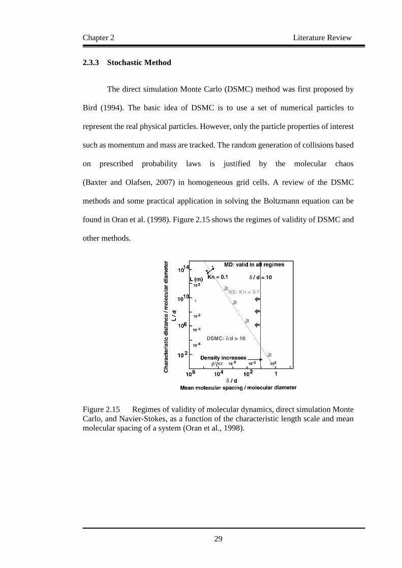
2.3.3 Stochastic Method 29
2.4 Direct Simulation Monte Carlo Method 30
2.4.1 Overview 30
2.4.2 Particle Representation 31
2.4.3 Algorithm and Numerical Simulation Parameters 32
2.5 Operator Splitting Monte Carlo Method 37
2.5.1 Overview 37
2.5.2 Operator Splitting Schemes 39
2.5.3 Implementation of Operator Splitting 41
2.6 Weighted Monte Carlo Methods 42
2.6.1 Overview 42
2.6.2 Different Weighting Numerical particles Schemes 43
2.7 CFD-Population Balance Modelling of Aerosol Dynamics 44
2.8 Transported PDF Methods for Turbulent Reactive Flows 46
2.8.1 Overview 46
2.8.2 Eulerian PDF methods 49
2.8.3 Lagrangian PDF Methods 52
2.8.4 Improvements of the PDF Methods 55

Table of Contents
vii
2.9 Summary of Literature Review 55
Chapter 3 Theoretical Fundamentals of the Present Study ……………… 58
3.1 Introduction 58
3.2 Population Balance Equation 58
3.2.1 Overview 58
3.2.2 The Self-preserving Behavior of PBE 60
3.2.3 The Solution of PBE 62
3.3 Monte Carlo Methods 64
3.3.1 Overview 64
3.3.2 Implementation Procedures 64
3.4 Eulerian-Lagrangian Models 65
3.4.1 Overview 65
3.4.2 Interphase Coupling 66
3.5 Transported PDF Methods for Turbulent Reactive Flows 67
3.5.1 Overview 67
3.5.2 Transport Equations for Turbulent Reactive Flows 68
3.5.3 Transported PDF Methods 68
3.6 Summary 69
Chapter 4 Zero-dimensional Monte Carlo Simulation of Aerosol
Dynamics ………………………………………………………. 70
4.1 Introduction 70
4.2 Numerical Methodology 71
4.2.1 General Dynamics Equation 71
4.2.2 Operator Splitting 72

Table of Contents
viii
4.2.3 Aerosol Dynamics Kernels 72
4.2.4 Non-dimensionalization 74
4.3 Numerical Setup 76
4.3.1 Time Step Determination 76
4.3.2 Integration Details 77
4.3.3 Initial Conditions and Cases with Analytical Solutions 79
4.3.3.1 Initial Conditions 79
4.3.3.2 Constant Rate Coagulation and Linear Rate Condensation 80
4.3.3.4 Simultaneous Coagulation, Nucleation and Condensation 81
4.3.4 Calculation of Maximum Relative Error 82
4.4 Results and discussion 82
4.4.1 Initial Validation 82
4.4.2 Constant Rate Coagulation and Nucleation 85
4.4.3 Free Molecular Regime Coagulation and Constant Rate Nucleation 87
4.4.4 Simultaneous coagulation, nucleation and condensation processes90
4.4.5 Parametric analysis of the studied cases 92
4.5 Summary 94
Chapter 5 CFD-PBM Simulation of Aerosol Dynamics in Turbulent
Flows ……………………………………………………………... 95
5.1 Introduction 95
5.2 Numerical Methodology 96
5.2.1 Governing Equations of Aerosol Dynamics in Turbulent Flows 96
5.2.2 PDF Transport Equation Formulation 99
5.2.2.1 Discretization of the Continuous PBE 99
Table of Contents
ix
5.2.2.2 Final PDF Transport Equation 101
5.2.3 Monte Carlo Simulation of the PDF Transport Equation 102
5.2.4 Simulation Analysis 106
5.3 Simulation Setup 107
5.4 Results and Discussion 111
5.4.1 Comparison of Coagulation in Both Laminar and Turbulent Flows 111
5.4.2 The Effect of Rej Number on Coagulation in Turbulent Flows 114
5.4.3 The Effect of Rej Number on Coagulation and Nucleation in
Turbulent Flows 119
5.4.4 Simultaneous Coagulation, Nucleation and Growth Processes in
Turbulent Flows 126
5.4.5 Computational Accuracy and Efficiency 131
5.4.6 Numerical Stability Analysis 133
5.5 Summary 134
Chapter 6 Simulation of Aerosol Dynamics in Turbulent Reactive flows.. 136
6.1 Introduction 136
6.2 Numerical Methodology 138
6.2.1 The CFD Code 138
6.2.2 The Lagrangian PDF Method 139
6.2.3 Particle Tracking Algorithm 141
6.2.4 Estimation of Mean Field 142
6.2.5 Soot Model 142
6.2.6 Radiation Model 143
6.3 Numerical Simulation Setup 144
Table of Contents
x
6.4 Results and Discussion 147
6.4.1 Axial and Radial Jet Temperature Variations of the Studied
Combustor 147
6.4.2 Axial and Radial Jet Mixture Fraction Variations of the Studied
Combustor 150
6.4.3 Axial and Radial Jet Soot Volume Fraction Variations of the Studied
Combustor 153
6.4.4 Soot Size Distribution 156
6.4.5 Relative Error Analysis 158
6.5 Summary 159
Chapter 7 Conclusions and Recommendations for Future Work ……… 161
7.1 Review of the Present Research 161
7.2 Main Conclusions of the Thesis 163
7.2.1 Conclusions of the Zero-Dimensional Monte Carlo Simulation of
Aerosol Dynamics 163
7.2.2 Conclusions of the CFD-PBM Simulation of Aerosol Dynamics in
Turbulent Flows 164
7.2.3 Conclusions of Simulation of Aerosol Dynamics in Turbulent
Reactive Flows 165
7.3 Recommendations for Future Work 166
7.3.1 Limitations of the Current Research 166
7.3.2 Recommendations for Future Work 167
Appendices ………………………………………………………………… 169
A.1 Coagulation Process 169
A.2 Nucleation Process 170
A.3 Surface Reactions in Soot Formation 170

Table of Contents
xi
A.4 Soot Formation Models 171
A.4.1 The One-Step Soot Formation Model 171
A.4.2 The Two-Step Soot Formation Model 172
A.4.2.1 Net Rate of Soot Generation 172
A.4.2.2 Net Rate of Nuclei Generation 173
A.4.3 The Moss-Brookes Model 174
A.4.4 The Moss-Brookes-Hall Model 175
References …………………………………………………………………. 177
List of Figures
xii
List of Figures
Figure 1.1 Modelling and simulation of multi-scale aerosol dynamics
(Kulmala et al., 2009).
2
Figure 1.2 Schematic diagram of the model to predict aerosol
formation in lower troposphere (MALTE) model
(Boy et al., 2006).
3
Figure 1.3 Schematic diagram of the aerosol dynamics, gas and
particle phase chemistry (ADCHEM) model
(Roldin et al., 2011).
4
Figure 1.4 A typical flow chart of Monte Carlo algorithm
(Efendiev, 2004).
6
Figure 1.5 A typical flow chart of direct simulation Monte Carlo
(DSMC) method (left) and Parallel DSMC method (right)
(Roohi and Darbandi, 2012).
8
Figure 2.1 Various mechanisms with cloud effects of atmospheric
aerosols (Valsaraj and Kommalapati, 2009).
17
Figure 2.2 Scatterplot of daily average PM2.5 concentrations from
continental U.S. monitoring stations for the period of
June 15−July 16, 1999 versus comparable CMAQ model
estimates (Byun and Schere, 2006).
17
Figure 2.3 Calculated distribution of a passive tracer released from a
surface point source using a fifth-order scheme in the
horizontal advection (Robertson et al., 1999).
18
Figure 2.4 Velocity vector profiles inside a fluidized bed reactor
obtained with computational fluid dynamics-discrete
element method (CFD-DEM) method (Zhuang et al., 2014).
19
Figure 2.5 Main reaction parameter distribution profiles in the
methanol to olefins (MTO) fluidized bed reactor (FBR) at
t = 0.052 s: (a) gas-phase temperature; (b) particle
temperature; (c) coke content; (d) ethane mole
concentration; (e) propene mole concentration; and
(f) butene mole concentration; space (velocity = 2.8 m/s,
inlet feed temperature = 723 K, feed ratio of water to
methanol = 0, adopted from Zhuang et al.(2014)).
20

List of Figures
xiii
Figure 2.6 Parallel Lattice Boltzmann simulation results for flow
within a fixed bed packed with the binary mixture of two
types of spheres: (a) velocity vector; and (b) velocity
contour and vector on the mid-plane (Rong et al., 2014).
21
Figure 2.7 Parallel Lattice Boltzmann simulation results for flow
within a fixed bed packed with the binary mixture of two
types of spheres: spatial distribution of the drag forces on
individual particle across the mid-plane (Rong et al., 2014).
21
Figure 2.8 (a) Computational domain using a purely atomistic
description; (b) Hybrid atomistic/continuum computational
domain; (c) Velocity field for the reference solution
averaged over 4 ns; and (d) Velocity field of the hybrid
solution after 50 iterations (Koumoutsakos, 2005).
22
Figure 2.9 The velocity profiles of flowing platelets in blood plasma
with a multi-scale method of dissipative particle dynamics
and coarse grained molecular dynamics (Zhang et al., 2014).
23
Figure 2.10 A schematic diagram of nano particles synthesis
(Balgis et al., 2014).
24
Figure 2.11 A schematic diagram of gas diffusion in nano structures
(Dreyer et al., 2014).
24
Figure 2.12 A schematic diagram of an online sampling system
(Zhao et al., 2003).
25
Figure 2.13 Comparison between sectional and analytic methods:
normalized number and volume concentrations under
constant coagulation and linear condensation
(Mitrakos et al., 2007).
27
Figure 2.14 The second order moment and the relative error for various
methods in the free molecular regime (Yu et al., 2008).
28
Figure 2.15 Regimes of validity of molecular dynamics, direct
simulation Monte Carlo, and Navier-Stokes, as a function
of the characteristic length scale and mean molecular
spacing of a system (Oran et al., 1998).
29
Figure 2.16 Operator splitting schemes: (a) first-order Lie scheme; and
(b) second-order Strang scheme (Zhou et al., 2014).
40

List of Figures
xiv
Figure 2.17 Flowchart of the operator splitting steps. (Xd and Xs have the
same meaning with those in Equation (2.9) (Zhou et al.,
2014).
41
Figure 2.18 Flow variables for the lth grid cell and four neighboring
cells in Eulerian PDF methods (Fox, 2003).
50
Figure 2.19 Flow diagram of Lagrangian PDF methods (Fox, 2003). 54
Figure 3.1 Computations of average population behavior via Monte
Carlo simulation (left) and PBE (right) (Ramkrishna, 2000). 63
Figure 3.2 Eulerian-Eulerian and Eulerian-Lagrangian multi-phase
models under different representations of the discrete phase
(Subramaniam, 2013).
65
Figure 4.1 Zeroth order moment, M0 under coagulation and
condensation processes for SWOSMC
(Liu and Chan, 2017) versus the analytical solution
(Ramabhadran et al., 1976) where N is the number of
numerical particles used in each simulation run.
83
Figure 4.2 First order moment, M1 under coagulation and condensation
processes for SWOSMC (Liu and Chan, 2017) versus the
analytical solution (Ramabhadran et al., 1976) where N is
the number of numerical particles used in each simulation
run.
84
Figure 4.3 Particle number density under free molecular regime
coagulation for SWOSMC (Liu and Chan, 2017) versus the
sectional method (Prakash et al., 2003) where the number
of numerical particles, N used in each simulation run is
1000.
85
Figure 4.4 Relative particle number density, N/N0 under constant rate
coagulation and nucleation processes for SWOSMC
(Liu and Chan, 2017) versus the analytical solution
(Maisels et al., 2004) where N is the number of numerical
particles used in each simulation run.
86
Figure 4.5 Relative particle volume concentration, V/V0 under constant
rate coagulation and nucleation processes for SWOSMC
(Liu and Chan, 2017) versus the analytical solution
(Maisels et al., 2004) where N is the number of numerical
particles used in each simulation run.
87
List of Figures
xv
Figure 4.6 Particle number density under free molecular regime
coagulation and constant rate nucleation for SWOSMC
(Liu and Chan, 2017) versus the sectional method
(Prakash et al., 2003) where N is the number of numerical
particles used in each simulation run.
88
Figure 4.7 Average diameter of the numerical particles, dave under
free molecular regime coagulation and constant rate
nucleation via SWOSMC (Liu and Chan, 2017) versus the
sectional method (Prakash et al., 2003) where N is the
number of numerical particles used in each simulation run.
89
Figure 4.8 Second order moment, M2 of the particles under free
molecular regime coagulation and constant rate nucleation
processes for SWOSMC (Liu and Chan, 2017) versus the
sectional method (Prakash et al., 2003) where N is the
number of numerical particles used in each simulation run.
90
Figure 4.9 Particle volume concentration, V/V0 under simultaneous
aerosol dynamic processes for SWOSMC
(Liu and Chan, 2017) versus the analytical solution
(Maisels et al., 2004) where the number of numerical
particles, N used in each simulation run is 4000.
91
Figure 4.10 Particle number concentration, N/N0 under simultaneous
aerosol dynamic processes for SWOSMC
(Liu and Chan, 2017) versus the analytical solution
(Maisels et al., 2004) where the number of numerical
particles, N used in each simulation run is 4000.
92
Figure 5.1 Flow chart of the coupled CFD-Monte Carlo/PDF method
(Liu and Chan, 2016).
105
Figure 5.2 Three-dimensional schematic configuration of a cylindrical
aerosol reactor (Two-dimensional axisymmetric grid is
generated in the rectangular domain ABCD, not in scale)
(Liu and Chan, 2016).
109
Figure 5.3 Two-dimensional axisymmetric unstructured
computational grid of a cylindrical aerosol reactor
(Liu and Chan, 2016).
110
Figure 5.4 Initial PSD of particles before entering the aerosol reactor
(Liu and Chan, 2016).
112
Figure 5.5 PSD in laminar and turbulent coagulation
(Liu and Chan, 2016).
112

List of Figures
xvi
Figure 5.6 Particle number density (m−3) contour in laminar and
turbulent coagulation (Liu and Chan, 2016).
113
Figure 5.7 PSD in turbulent coagulation: Case A, Rej=3200; Case B,
Rej=4800; Case C, Rej=6400; Case D, Rej=12800
(The PBSM results are obtained based on the method
proposed by Hounslow (1988)) (Liu and Chan, 2016).
114
Figure 5.8 Average diameter of particles in turbulent coagulation
(Liu and Chan, 2016).
115
Figure 5.9 Turbulent kinetic energy (m2/s2) contour in turbulent
coagulation (Liu and Chan, 2016).
117
Figure 5.10 Particle number density (m−3) contour in turbulent
coagulation (Liu and Chan, 2016).
118
Figure 5.11 Normalized particle number density of turbulent
coagulation (Liu and Chan, 2016).
119
Figure 5.12 PSD of simultaneous coagulation and nucleation in
turbulent flows: Case A, Rej=3200; Case B, Rej=4800;
Case C, Rej=6400; Case D, Rej=12800 (The PBSM results
are obtained based on the method proposed by Hounslow
(1988)) (Liu and Chan, 2016).
120
Figure 5.13 Average diameter of particles for coagulation and
nucleation in turbulent flows (Liu and Chan, 2016).
122
Figure 5.14 Turbulent kinetic energy (m2/s2) contour for simultaneous
coagulation and nucleation in turbulent flows
(Liu and Chan, 2016).
123
Figure 5.15 Particle number density (m−3) contour for simultaneous
coagulation and nucleation in turbulent flows
(Liu and Chan, 2016).
124
Figure 5.16 Normalized particle number density for simultaneous
coagulation and nucleation in turbulent flows
(Liu and Chan, 2016).
125
Figure 5.17 PSD for simultaneous coagulation, nucleation and growth
in turbulent flows: Case A, Rej=3200; Case B, Rej=4800;
Case C, Rej=6400; Case D, Rej=12800 (The PBSM results
are obtained based on the method proposed by Hounslow
(1988)) (Liu and Chan, 2016).
127
List of Figures
xvii
Figure 5.18 Average diameter of particles for simultaneous coagulation,
nucleation and growth in turbulent flows
(Liu and Chan, 2016).
128
Figure 5.19 Particle number density (m−3) contour for simultaneous
coagulation, nucleation and growth in turbulent flows
(Liu and Chan, 2016).
129
Figure 5.20 Normalized particle number density for simultaneous
coagulation, nucleation and growth in turbulent flows
(Liu and Chan, 2016).
130
Figure 6.1 Jet burner configuration of the combustor
(Brookes and Moss, 1999).
145
Figure 6.2 The computational grid used in the numerical simulation of
an axisymmetric combustor.
146
Figure 6.3 Axial jet temperature variation at the centerline of the
studied combustor for Rej= 5000 (The experimental results
are obtained from Brookes and Moss (1999)).
148
Figure 6.4 Radial jet temperature variation at the axial distance of 250
mm for the studied combustor at Rej= 5000
(The experimental results are obtained from Brookes and
Moss (1999)).
149
Figure 6.5 Radial jet temperature variation at the axial distance of
350 mm for the studied combustor at Rej= 5000
(The experimental results are obtained from Brookes and
Moss (1999)).
150
Figure 6.6 Axial jet mixture fraction variation at the centerline of the
studied combustor for Rej= 5000 (The experimental results
are obtained from Brookes and Moss (1999)).
151
Figure 6.7 Radial jet mixture fraction variation at the axial distance of
250 mm for the studied combustor at Rej= 5000
(The experimental results are obtained from Brookes and
Moss (1999)).
152
Figure 6.8 Radial jet mixture fraction variation at the axial distance of
350 mm for the studied combustor at Rej= 5000
(The experimental results are obtained from Brookes and
Moss (1999)).
153
List of Figures
xviii
Figure 6.9 Axial jet soot volume fraction variation at the centerline of
the studied combustor for Rej= 5000 (The experimental
results are obtained from Brookes and Moss (1999)).
154
Figure 6.10 Radial jet soot volume fraction variation at the axial
distance of 350 mm for the studied combustor at Rej= 5000
(The experimental results are obtained from Brookes and
Moss (1999)).
155
Figure 6.11 Radial jet soot volume fraction variation at the axial
distance of 425 mm for the studied combustor at Rej= 5000
(The experimental results are obtained from Brookes and
Moss (1999)).
156
Figure 6.12 PSD of jet soot particles at the axial distances of 138 mm
and 308 mm (The benchmark results are from Akridis and
Rigopoulos (2015)).
157

List of Tables
xix
List of Tables
Table 2.1 Typical physical properties of atmospheric aerosols
(Valsaraj and Kommalapati, 2009).
16
Table 2.2 Mass concentrations and diameters of atmospheric
aerosols (Valsaraj and Kommalapati, 2009).
16
Table 4.1 A comparison between the developed SWOSMC
method and analytical solutions.
71
Table 4.2 Summary of the studied cases (Liu and Chan, 2017). 80
Table 4.3 Analysis of main simulation parameters (Liu and Chan,
2017).
93
Table 5.1 Simulation parameters for aerosol dynamics in turbulent
flows (Liu and Chan, 2016).
110
Table 5.2 Maximum relative error and normalized convergence
time for different studied cases (Liu and Chan, 2016).
132
Table 5.3 Typical grid cell independence analysis. 133
Table 5.4 Typical analysis of the number of simulation particles
per grid cell.
134
Table 6.1 Model constants for the k-ε turbulence model. 139
Table 6.2 Jet burner parameters and conditions for the studied
combustor.
145
Table 6.3 Relative error analysis between the present numerical
and experimental results (Brookes and Moss, 1999).
159
Nomenclature
xx
Nomenclature
a subscript of ordering
a0* pre-exponential rate constant
ap Planck mean absorption coefficient, s2/kg
A unspecified operator
As area of soot particle, m2
Asoot constant in the Magnussen model
b* normalized radical nuclei concentration, particle10−15/kg
B dimensionless parameter
Bn nucleation kernel, m3/s
c the constant factor used to adjust time step
cfuel fuel concentraion, kg/m3
cnuc radical nuclei concentration, #/m3
c*nuc normalized nuclei concentration
C dimensionless model constant
CI dimensionless nucleation constant related to diffusion and
temperature
Cmin minimum number of carbon atoms for the incipient soot
cp specific heat capacity, J/(kg∙K)
dave average diameter of particles, m
dp particle diameter, m
Dp diffusion coefficients of particles , m2/s

Nomenclature
xxi
E dimensionless parameter
Ea activation energy, kJ/mol
f unspecified function
(f g)soot linear branching-termination coefficient, 1/s
fv volume fraction of soot particles
fU,ψ joint composition and velocity PDF
fU joint velocity PDF
fψ joint composition PDF
F fine-grained density function
g0 linear termination on soot particles, m3/(particle-s).
G particle growth kernel, m/s
G0 the reduction rate of the smallest size particles by coagulation, #/s
GO2 particle oxidation rate of oxygen (O2), #/(m2∙s)
GOH particle oxidation rate of hydroxide (OH), #/(m2∙s)
GSG particle growth rate, m/s
Gt generation rate of turbulent kinetic energy, m2/s3
H source of energy, J
h small time interval, s
i subscript of ordering
I particle condensation kernel, 1/(m3∙s)
j subscript of ordering
k turbulent kinetic energy, m2/s2

Nomenclature
xxii
kB Boltzmann constant, J/K
ke heat conductivity, m2/s
kn reaction constant of nucleation, #/(m3∙s)
ks the reaction rate per unit area, #/(m2∙s)
kHW reaction constant of growth, #/(m∙s)
ka,kb reaction constant of oxidation, #/(m2∙s)
K coagulation kernel
Kn Knudsen number
l model exponent constant
Lj internal coordinate in the physical and scalar space
mp mass of the particle, p, kg
M a vector space
Mj rate of certain aerosol dynamic process, j
Mp mass of an incipient soot particle, kg
n number density of aerosol particles, #/m3
N particle number concentration, #/m3
NA Avogadro constant, 1/mol
NCFL local CFL number in the computational domain
Ng0 the number density of newly generated smallest size particles
Nl local concentration of particles, #/m3
Nn normalized particle number density
Nnorm reference number density of soot particles, particle10−15/m3
Nomenclature
xxiii
N0 initial particle number concentration, #/m3
N∞ total number of particles in the system
NU0 nucleation rate, #/(m3∙s)
p particle phase
P pressure, kg/(m∙s2)
pfuel fuel partial pressure, Pa
q mass density of aerosol particles, kg/m3
q relative mass density of aerosol particles, kg/kg
Q total mass of aerosol particles, kg
Qc, physical quantity in a cell, c
Qp physical quantity carried by particle, p
Qrad the source term due to radiation
Qlaminar the volumetric flow rate of laminar flow
Qturbulent the volumetric flow rate of turbulent flow
r equivalence ratio exponent
R universal gas constant, J/(mol∙K)
R*nuc normalized net rate of nuclei generation,
particle10−15/(m3⋅s)
R0 reduction rate that creates the smallest size particles, #/s
Rsoot net rate of soot generation, kg/(m3∙s)
Rsoot,form soot formation rate, kg/(m3∙s)
Rsoot, combst soot combustion rate, kg/(m3∙s)

Nomenclature
xxiv
Rej Reynolds number of the jet based on the nozzle diameter
s molecular ratio of fuel to oxidizer
S0 the surface area of the smallest size particles, m2
Sa the source term due to chemical reaction
t time, s
rms root mean square
T endpoint of a time interval, s
Tα activation temperature for nucleation reaction, K
Tγ activation temperature for surface growth reaction, K
Tω activation temperature for oxidation reaction, K
Ttemp temperature, K
u particle volume, m3
u velocity of carrier fluid phase, m/s
v particle volume, m3
vsoot, vfuel mass stoichiometries for soot and fuel combustion, respectively
v average particle volume, m3
�� velocity space in PDF
V total volume of the aerosol system in simulation, m3
V0 initial volume of the aerosol system in simulation, m3
Vs volume of a subsystem of aerosol particles, m3
w particle mass weight, kg/kg
Nomenclature
xxv
W
Wd
Wiener process
operator of deterministic process
WH2 molecular weight of hydrogen, g/mol
WC2H2 molecular weight of acetylene, g/mol
WC6H5 molecular weight of benzene radical, g/mol
WC6H6 molecular weight of benzene, g/mol
WP particle weight
Ws operator of stochastic process
X the position of notional particles
Xd deterministic process
Xprec mole fraction of soot precursor, mol/mol
Xs stochastic process
Xsgs the mole fraction of the participating surface growth species,
mol/mol
y size of aerosol particles, m3
Y mass fraction of aerosol particles, kg/kg
YO,YF molecular fraction of oxidizer and fuel, respectively.
Yox,Yfuel mass fractions of oxidiser and fuel, respectively, kg/kg
Ysoot soot mass fraction, kg/kg
Z mixture fraction in the jet flame

Nomenclature
xxvi
Greek Symbols
α empirical constant
coagulation kernel, m3/s
Γ turbulent diffusivity, m2/s
∆m mass change during a single reaction event, kg
δ Kronecker delta function
ε turbulent dissipation rate, m2/s3
max maximum relative error
ηcoll collision efficiency
ηv dimensionless particle volume, m3/m3
ηd dimensionless particle diameter
μ molecular viscosity, kg/(m⋅s)
μt turbulent viscosity
νk kinematic viscosity, m2/s
ρ mass density, kg/m3
σk, σε turbulent Prandtl number
σnuc turbulent Prandtl number for nuclei transport
σs the Stefan-Boltzmann constant, kg/(s3⋅K4)
σsoot turbulent Prandtl number for soot transport
τ dimensionless time
Nomenclature
xxvii
ϕ total volume of particles in the system
ϕα unspecified reacting scalar
ϕcombst equivalence ratio for combustion process
Φ micro-mixing term
ψ composition space in PDF
ψv dimensionless function of particle volume
ψd dimensionless function of particle diameter
ω weight of numerical particles
Abbreviations
ADCHEM aerosol dynamics, gas and particle phase chemistry
CFD computational fluid dynamics
CFL Courant–Friedrichs–Lewy condition
CMAQ community multi-scale air quality modeling systems
3D-CTM three-dimensional chemical transport model
DEM discrete element method
DGM dusty gas model
DSMC direct simulation Monte Carlo
DPD dissipative particle dynamics
EMST Euclidean minimum spanning tree
FBR fluidized bed reactor
GCM multi-scale global aerosol-climate model
Nomenclature
xxviii
GDE general dynamics equation
GHS generalized variable hard sphere model
HS hard sphere model
IC internal combustor
LBM Lattice Boltzmann method
LMC-PDF Lagrangian Monte Carlo-probability density function
LPDA linear process deferment algorithm
MALTE model to predict aerosol formation in lower troposphere
MATCH multi-scale atmospheric transport and chemistry model
MC Monte Carlo method
MCMC Markov chain Monte Carlo method
MD molecular dynamics
MFA mass flow algorithm
MP-PIC multi-phase particle in cell
MTO methanol to olefins
ODE ordinary differential equations
OSMC operator splitting Monte Carlo method
PBE population balance equation
PDE partial differential equation
PBM population balance method
PBSM population balance sectional method
PDF probability density function
PSD particle size distribution

Nomenclature
xxix
PSI-Cell particle source in cell
DQMOM direct quadrature method of moments
RANS Reynolds averaged Navier-Stokes equation
SDE stochastic differential equation
SEF stochastic Eulerian field method
SEM scanning electron microscopy
SWOSMC stochastically weighted operator splitting Monte Carlo
method
SWPM stochastically weighted particle method
TCI turbulence chemistry interaction
TRI turbulence radiation interation
TEM transmission electron microscopy
TEMOM Taylor-series expansion method of moments
Chapter 1 Introduction
1
Chapter 1 Introduction
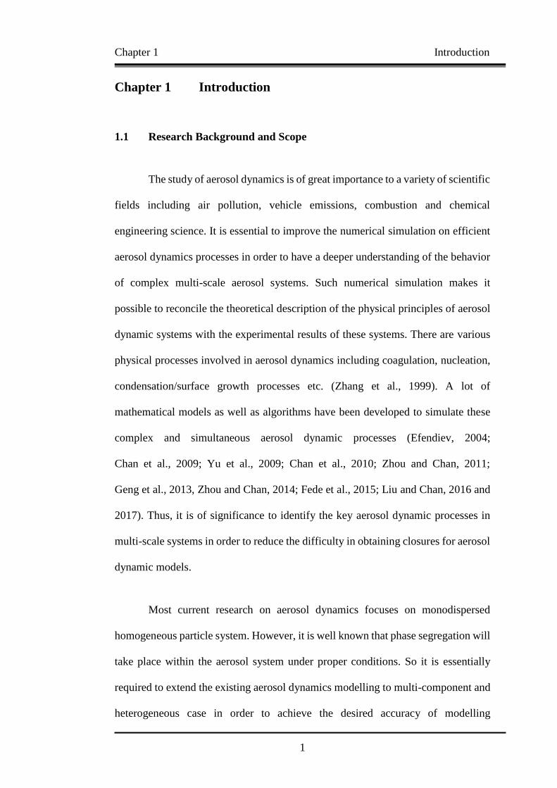
1.1 Research Background and Scope
The study of aerosol dynamics is of great importance to a variety of scientific
fields including air pollution, vehicle emissions, combustion and chemical
engineering science. It is essential to improve the numerical simulation on efficient
aerosol dynamics processes in order to have a deeper understanding of the behavior
of complex multi-scale aerosol systems. Such numerical simulation makes it
possible to reconcile the theoretical description of the physical principles of aerosol
dynamic systems with the experimental results of these systems. There are various
physical processes involved in aerosol dynamics including coagulation, nucleation,
condensation/surface growth processes etc. (Zhang et al., 1999). A lot of
mathematical models as well as algorithms have been developed to simulate these
complex and simultaneous aerosol dynamic processes (Efendiev, 2004;
Chan et al., 2009; Yu et al., 2009; Chan et al., 2010; Zhou and Chan, 2011;
Geng et al., 2013, Zhou and Chan, 2014; Fede et al., 2015; Liu and Chan, 2016 and
2017). Thus, it is of significance to identify the key aerosol dynamic processes in
multi-scale systems in order to reduce the difficulty in obtaining closures for aerosol
dynamic models.
Most current research on aerosol dynamics focuses on monodispersed
homogeneous particle system. However, it is well known that phase segregation will
take place within the aerosol system under proper conditions. So it is essentially
required to extend the existing aerosol dynamics modelling to multi-component and
heterogeneous case in order to achieve the desired accuracy of modelling
Chapter 1 Introduction
2
(Efendiev, 2004). A large number of studies concerning complex aerosol dynamics
and applications have been reported (Efendiev, 2002; Efendiev, 2004; Fu et al., 2012;
Gac and Gradoń, 2013; Trump et al., 2015; Feng et al., 2016).
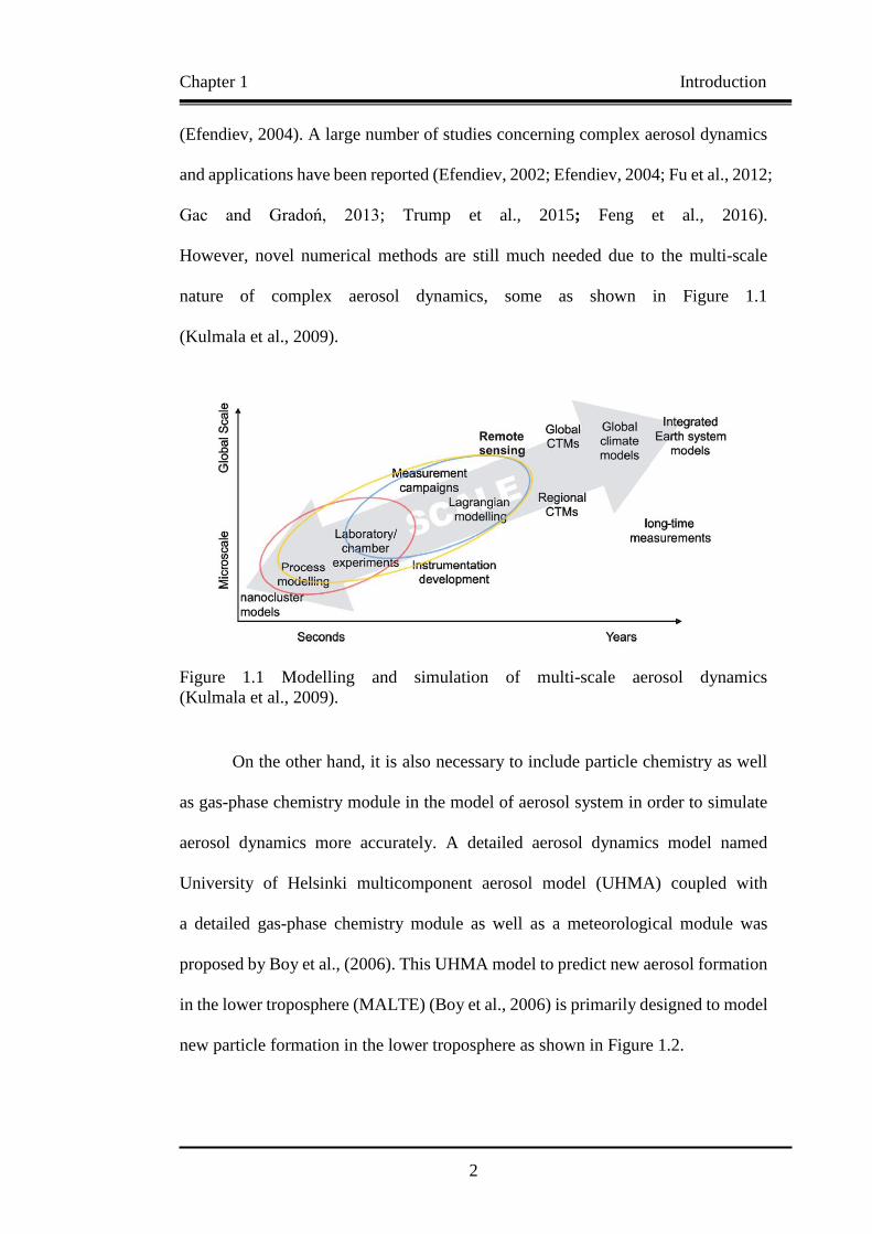
However, novel numerical methods are still much needed due to the multi-scale
nature of complex aerosol dynamics, some as shown in Figure 1.1
(Kulmala et al., 2009).
Figure 1.1 Modelling and simulation of multi-scale aerosol dynamics
(Kulmala et al., 2009).
On the other hand, it is also necessary to include particle chemistry as well
as gas-phase chemistry module in the model of aerosol system in order to simulate
aerosol dynamics more accurately. A detailed aerosol dynamics model named
University of Helsinki multicomponent aerosol model (UHMA) coupled with
a detailed gas-phase chemistry module as well as a meteorological module was
proposed by Boy et al., (2006). This UHMA model to predict new aerosol formation
in the lower troposphere (MALTE) (Boy et al., 2006) is primarily designed to model
new particle formation in the lower troposphere as shown in Figure 1.2.

Chapter 1 Introduction
3
Figure 1.2 Schematic diagram of the model to predict aerosol formation in lower
troposphere (MALTE) model (Boy et al., 2011).
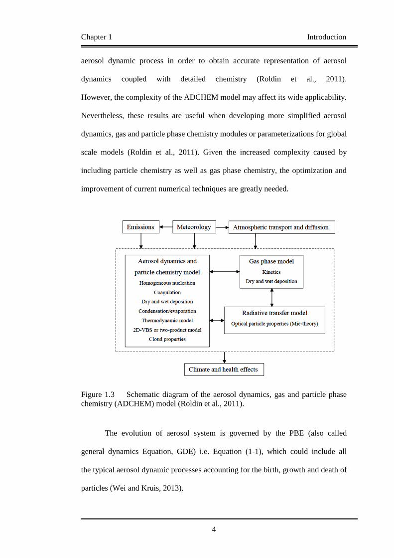
A more detailed and comprehensive model including aerosol dynamics,
gas and particle phase CHEMistry and radiative transfer (ADCHEM)
(Roldin et al., 2011) as shown in Figure 1.3 is then proposed based on the developed
MALTE model. The aim of the ADCHEM model was to develop a model suitable
for the investigation of multi-scale complex aerosol dynamics coupled with gas and
particle chemistry. The ADCHEM model was used to identify the most important
Chapter 1 Introduction
4
aerosol dynamic process in order to obtain accurate representation of aerosol
dynamics coupled with detailed chemistry (Roldin et al., 2011).
However, the complexity of the ADCHEM model may affect its wide applicability.
Nevertheless, these results are useful when developing more simplified aerosol
dynamics, gas and particle phase chemistry modules or parameterizations for global
scale models (Roldin et al., 2011). Given the increased complexity caused by
including particle chemistry as well as gas phase chemistry, the optimization and
improvement of current numerical techniques are greatly needed.
Figure 1.3 Schematic diagram of the aerosol dynamics, gas and particle phase
chemistry (ADCHEM) model (Roldin et al., 2011).
The evolution of aerosol system is governed by the PBE (also called
general dynamics Equation, GDE) i.e. Equation (1-1), which could include all
the typical aerosol dynamic processes accounting for the birth, growth and death of
particles (Wei and Kruis, 2013).
Chapter 1 Introduction
5
∂n(v,t) ∂t⁄ = 1 2⁄ ∫ β(vu,u)n(u,t)n(vu,t)du n(v,t) ∫ β(v,u)n(u,t)du∞
0
v
0 (1-1)
where n(v,t) is the particle size distribution (PSD) at time t and β(v,u) is
the coagulation rate for two particles with the volumes u and v, respectively.
The first term on the right-hand side of Equation (1-1) represents the formation of
particles with volume v due to the coagulation events between particles of volume u
and particles of volume (v-u); the factor 1/2 is introduced because the collisions are
counted twice for a single collision event. The second term on the right-hand side of
Equation (1-1) represents the loss of particles with volume v because of collisions
with particles of other sizes.
There are different numerical methods to solve the Equation (1-1),
including sectional methods (Jeong and Choi, 2001; Mitrakos et al., 2007;
Agarwal and Girshick, 2012), methods of moments (Lin and Chen, 2013;
Yu et al., 2008; Park et al., 2013; Chen et al., 2014; Yu and Chan, 2015;
Pollack et al., 2016), and Monte Carlo methods (Zhao et al., 2009; Zhao and Zheng,
2012; Wei, 2013; Zhou et al., 2014; Liu et al., 2015; Liu and Chan, 2016).
The computational time of sectional methods is moderate, but the algorithms for the
sectional representations could be quite complicated (Wei and Kruis, 2013).
Methods of moments have relatively high computational efficiency, but require
input of the initial PSD, which is variable during the numerical simulation,
particularly when another aerosol dynamic process like nucleation takes place
(Wei and Kruis, 2013). The methods of moment perform best only when the size
distribution is lognormal. Besides these two deterministic methods, the Monte Carlo
method with a stochastic nature is considered feasible to deal with the multi-scale
Chapter 1 Introduction
6
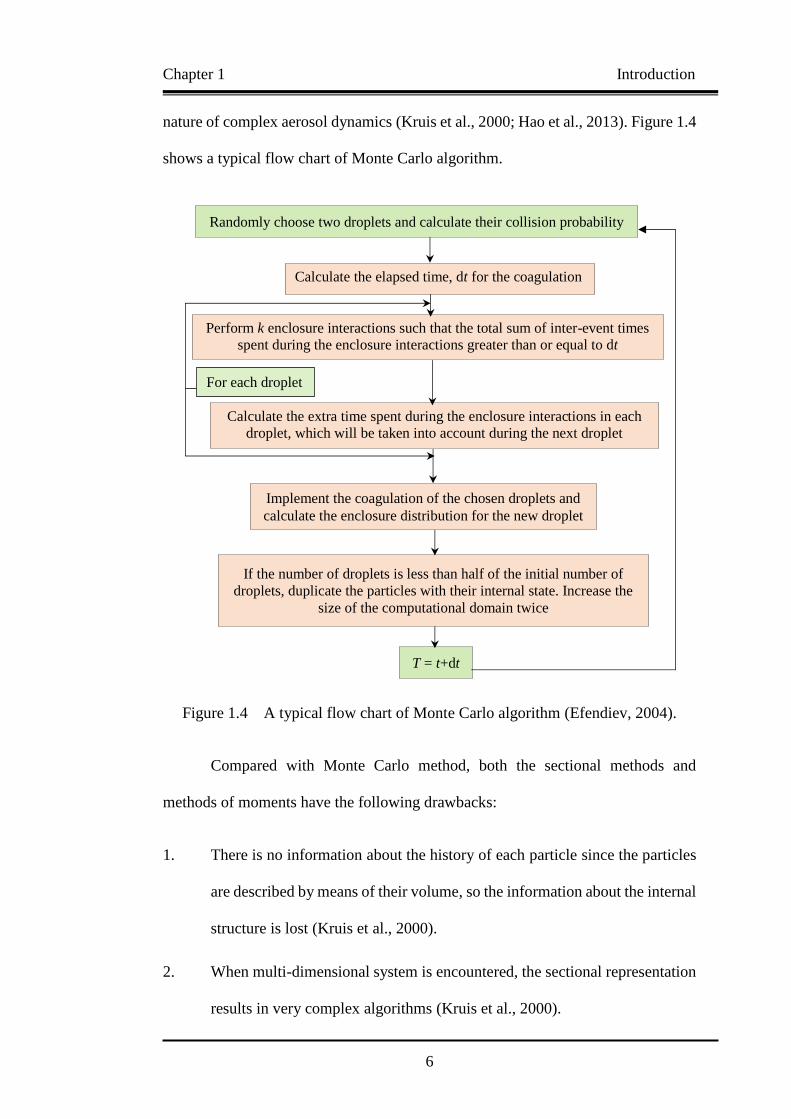
nature of complex aerosol dynamics (Kruis et al., 2000; Hao et al., 2013). Figure 1.4
shows a typical flow chart of Monte Carlo algorithm.
Figure 1.4 A typical flow chart of Monte Carlo algorithm (Efendiev, 2004).
Compared with Monte Carlo method, both the sectional methods and
methods of moments have the following drawbacks:
1. There is no information about the history of each particle since the particles
are described by means of their volume, so the information about the internal
structure is lost (Kruis et al., 2000).
2. When multi-dimensional system is encountered, the sectional representation
results in very complex algorithms (Kruis et al., 2000).
For each droplet
Randomly choose two droplets and calculate their collision probability
Calculate the elapsed time, dt for the coagulation
event
Perform k enclosure interactions such that the total sum of inter-event times
spent during the enclosure interactions greater than or equal to dt
Calculate the extra time spent during the enclosure interactions in each
droplet, which will be taken into account during the next droplet coagulation event
Implement the coagulation of the chosen droplets and
calculate the enclosure distribution for the new droplet
If the number of droplets is less than half of the initial number of
droplets, duplicate the particles with their internal state. Increase the
size of the computational domain twice
T = t+dt

Chapter 1 Introduction
7
Monte Carlo simulation is a classical method to be used to overcome
the above drawbacks. The major shortcomings of the Monte Carlo methods are
the high computational cost (i.e., computational time, computer memory etc.)
required in order to obtain satisfactory accuracy. This is because Monte Carlo
methods are essentially stochastic methods and the computational error is inversely
proportional to the square root of the total number of the numerical particles
(Oran et al., 1998).
High performance computing (HPC) clusters are thus used in order to reduce
the high computational cost (i.e., computational time, computer memory etc.) at high
expense. Moreover, the development of parallel computing technique makes it
possible to use many-core processors for Monte Carlo simulation, in which parallel
computing is applied to stochastic processes (Wei and Kruis, 2013).
Since the Direct Simulation Monte Carlo (DSMC) method is a stochastic
particle method, the movement of particles is independent of each other except for
the inter-particle collisions (Wu and Lian, 2003). Thus, it is inherently justified to
execute the DSMC method using the parallel processors in order to reduce
computational time (Wu and Lian, 2003; Mohammadzadeh et al., 2013).
A typical flow chart of parallel DSMC algorithm is shown in Figure 1.5
(Roohi and Darbandi, 2012).

Chapter 1 Introduction
8
Figure 1.5 A typical flow chart of direct simulation Monte Carlo (DSMC) method
(left) and parallel DSMC method (right) (Roohi and Darbandi, 2012).
Another method to accelerate the conventional Monte Carlo simulation
which selects all processes (i.e., nucleation, surface growth and coagulation)
randomly at a time, the new methods of Linear Process Deferment (LPDA) and
Operator Splitting Monte Carlo (OSMC) are proposed by Patterson et al. (2006) and
Zhou et al. (2014), respectively, which separates coagulation from other nucleation
Chapter 1 Introduction
9
and surface growth processes. In most of the conventional Monte Carlo methods,
every simulation particle is associated with the uniform number of real particles.
The accuracy of the simulation thus depends on the number of numerical particles
used. Hence, it decreases the applicability of Monte Carlo method to the spatially
resolved gas simulations, and regions with few physical particles cannot be modeled
accurately. A stochastically weighted particle method (SWPM) is thus introduced
by Rjasanow and Wagner (1996) to deal with this problem of simulation accuracy.
A new stochastically weighted operator splitting Monte Carlo (SWOSMC) method
based on the idea of operator splitting and a stochastic weight for every simulation
particle is newly proposed in the present study. The purpose of this new method aims
to solve complex aerosol dynamic problems with high accuracy and efficiency,
which will provide a better knowledge of the evolution of aerosol system and a better
deal with the multi-scale, multi-component and heterogeneous aerosol dynamics
with high performance computing. In fact, parallel DSMC method has been studied
and implemented in many fields such as multiphase flow, aerosol coagulation
phenomena; molecular dynamics etc. (Kruis et al., 2000; Liffman, 1992;
Mohammadzadeh et al., 2013). In the present study, further research development
of implementing this new SWOSMC method to multi-scale aerosol systems will be
presented.
However, in actual industrial and engineering applications,
an inhomogeneous flow field is generally encountered which has a profound impact
on aerosol dynamic processes. Those processes are dependent on local flow field
variables (e.g., temperature and concentration). Thus, the solution for
multidimensional PBE including convection and diffusion terms becomes

Chapter 1 Introduction
10
significant for aerosol dynamics in turbulent flow. Coupling the PBE of aerosol
dynamics with CFD method provides a very promising approach to deal with
the spatially inhomogeneous problems of aerosol dynamics (Kruis et al., 2012;
Zhao and Zheng, 2013; Zhou and Chan, 2014; Zhou and He, 2014;
Akridis and Rigpoulos, 2015; Amokrane et al., 2016). In laminar flow, the coupling
of CFD to PBE can be easily accomplished via proper transformation of PBE.
However, in turbulent flow, the closure problems arise due to the effect of turbulence
on aerosol dynamic processes (e.g. coagulation, nucleation and growth) as such
physical processes are highly dependent on the local field variables.
Moreover, the relationship between turbulence, particle properties and collision
kernels of aerosol dynamics is not well understood and is rarely reported due to their
theoretical and experimental limitations (Lesniewski and Friedlander, 1995;
Reade and Collins, 2000; Rigopoulos, 2007; Balachadar and Eaton, 2010;
Minier, 2015). Thus, particular attention is paid to examine the effect of turbulence
on aerosol dynamics and the evolution of PSD of aerosol dynamics in the present
study.
Probability density function (PDF) methods based on a PDF transport
equation of the full PSD have been proposed and used to overcome the closure
problems due to interaction between turbulence and particle evolution in turbulent
reactive flows (Pope, 1981; Pope, 1985; Valino, 1998; Sabel’nikov and Soulard,
2005; Meyer, 2010; Pope and Tirunagari, 2014; Consalvi and Nmira, 2016).
Both PSD and particle number density distribution are treated without additional
assumptions for closure via the transported PDF methods. The full PSD can thus be
obtained directly without reconstructing it from moments. Moreover, complex and

Chapter 1 Introduction
11
arbitrary kernels of aerosol dynamics are allowed since no closure is required for
the PBE. These PDF methods can be divided into three categories i.e.,
Eulerian particle method (Pope, 1981), Lagrangian particle method (Pope, 1985) and
Eulerian field method (Sabel’nikov and Soulard, 2005). Both the advantages and
disadvantages of the methods and possible improvements can easily be identified in
the comparison between Eulerian and Lagrangian Monte Carlo PDF methods
(Möbus et al., 2001; Zhang and Chen, 2007; Haworth, 2010; Jaishree and Haworth,
2012).
Lagrangian particle Monte Carlo algorithms (Pope, 1985; Jaishree and
Haworth, 2012) have been regarded as the mainstream approach for solving PDF
transport equations in most applications of PDF methods to date (Haworth, 2010;
Haworth and Pope, 2011). A great number of notional particles that evolve according
to the prescribed stochastic differential equations (SDE) (Celis and Silva, 2015)
represents the PDF, and weighted averages over the particles in a small amount of
neighboring grids are used to approximate the local mean quantities. As the mean
velocity and turbulence scales are required before advancing in every time step,
it is necessary to couple the Lagrangian particle method with a conventional CFD
solver to formulate a consistent hybrid Lagrangian particle/Eulerian mesh PDF
method (Jaishree and Haworth, 2012; Jangi et al., 2015). The main advantage of
Lagrangian particle method relative to Eulerian PDF method is that the spatial-
transport algorithm has much higher accuracy. The number of grid cells required for
equivalent accuracy is thus considerably smaller and the total computational cost
(i.e., computational time, computer memory etc.) of Lagrangian PDF is only
proportional to the number of notional particles despite the special care required for

Chapter 1 Introduction
12
reducing statistical error. A consistent hybrid Lagrangian particle /Eulerian mesh
PDF method (Jaishree and Haworth, 2012; Jangi et al., 2015) based on the work of
Pope (1985) is proposed for the coupled CFD-Monte Carlo simulation of aerosol
dynamics in turbulent flow in the present study. Further application of the coupled
CFD-Monte Carlo method to turbulent reactive flows is also studied in the following
content.
1.2 Research Motivation and Objectives
In the present study, a stochastically weighted operator splitting Monte Carlo
(SWOSMC) method is first formulated based on the improvement of Monte Carlo
(MC) method with the coupling of operator splitting technique and stochastic weight
method. Then the SWOSMC method is coupled to computational fluid dynamics
(CFD) in terms of Lagrangian probability density function (PDF) representation
approximating the discretized population balance equation (PBE).
The objectives of the present study are as follows:
1. To gain a better understanding of the aerosol dynamic processes such as
coagulation, nucleation, condensation etc. in aerosol dynamics in turbulent
flows by the development of the stochastically weighted operator splitting
Monte Carlo (SWOSMC) method;
2. To develop a novel coupled CFD-Monte Carlo/PDF method for spatially
inhomogeneous aerosol dynamic system in turbulent flows with wide
applicability by combining with a CFD method to formulate a CFD-based

Chapter 1 Introduction
13
aerosol dynamics method with applications to complex particle-fluid
systems; and
3. To extend the CFD-Monte Carlo/PDF method for the application to turbulent
reactive flows by including a chemical reactions module in this method.
4. This newly proposed CFD-Monte Carlo/PDF method is expected to render
an efficient method for simulating complex aerosol dynamics in turbulent
reactive flows and provides a better insight into the interaction between
turbulence and the full PSD of aerosol particles.
1.3 Outline of the Thesis
Chapter 1 introduces an overview of the background and scope related to
the present study, indicating that the knowledge gap of the numerical simulation of
multi-scale interaction of complex aerosol dynamics in polydispersed turbulent
reactive flows. The objectives of the present study are intended to fill this knowledge
gap.
Chapter 2 provides a more detailed literature review of aerosol dynamics
including the knowledge of aerosol dynamics obtained via the experimental and
numerical studies, indicating the development and state-of-the-art that
the researchers have acquired, and the shortcomings of these research areas and
where the knowledge gap lies.
Chapter 1 Introduction
14
Chapter 3 provides theoretical fundamentals of the present study,
which contains necessary mathematical and numerical models that will be used in
Chapters 4 to 6.
Chapter 4 provides this newly proposed SWOSMC method with its
validation and applications to simultaneous complex aerosol dynamics.
Chapter 5 presents this newly proposed CFD-Monte Carlo/PDF method
with applications to the study of interaction between turbulence and aerosol
dynamics in turbulent flows.
Chapter 6 provides the extension of this proposed and developed
CFD-Monte Carlo method to turbulent reactive flows by including a chemical
reaction module. This method is then used to study the soot formation in
non-premixed turbulent reactive flows.
Chapter 7 provides the conclusions and major scientific findings revealed
by the present study, and some recommendations for future work.
Chapter 2 Literature Review
15
Chapter 2 Literature Review
2.1 Aerosol Dynamics in Multi-scale Systems
There are miscellaneous multi-scale systems concerning aerosol dynamics in
nature as well as in human activities. Some typical examples regarding the aerosol
dynamics in multi-scale systems will be reviewed briefly in the following sections.
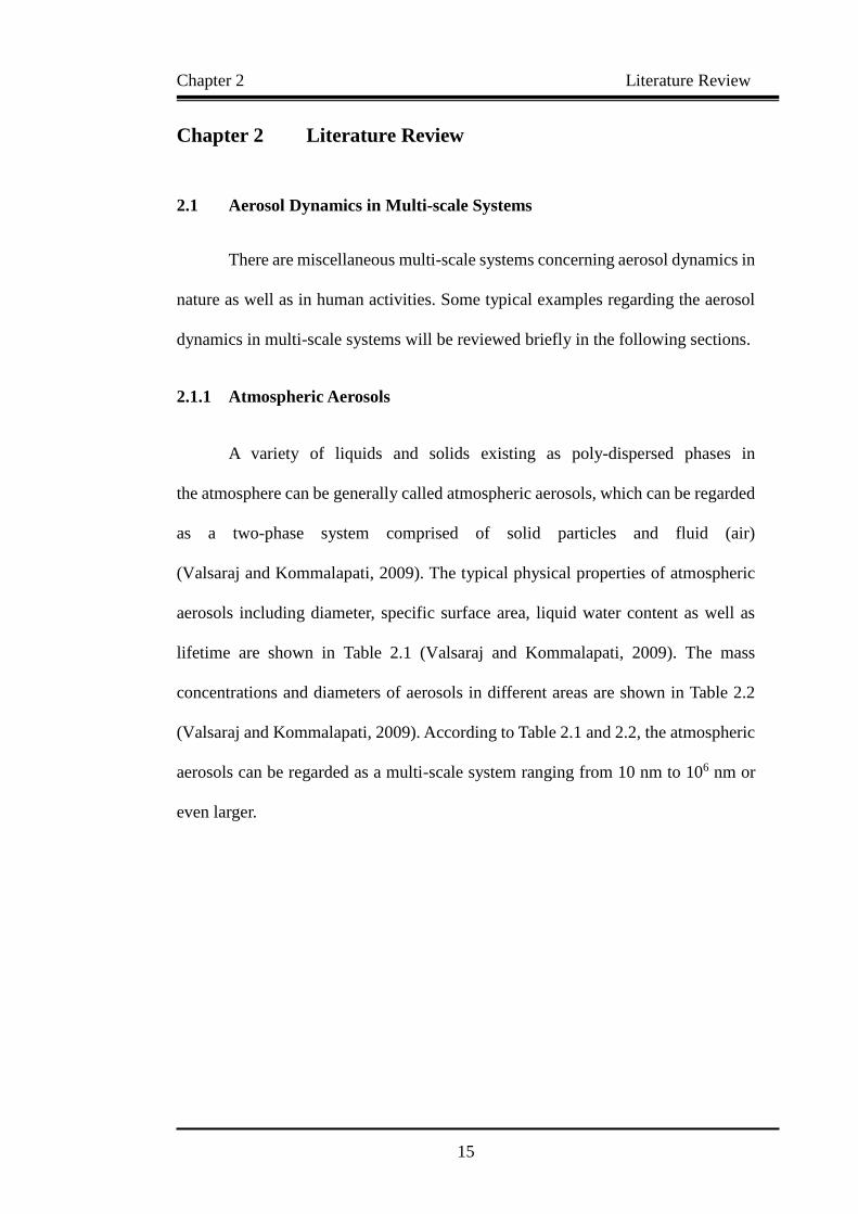
2.1.1 Atmospheric Aerosols
A variety of liquids and solids existing as poly-dispersed phases in
the atmosphere can be generally called atmospheric aerosols, which can be regarded
as a two-phase system comprised of solid particles and fluid (air)
(Valsaraj and Kommalapati, 2009). The typical physical properties of atmospheric
aerosols including diameter, specific surface area, liquid water content as well as
lifetime are shown in Table 2.1 (Valsaraj and Kommalapati, 2009). The mass
concentrations and diameters of aerosols in different areas are shown in Table 2.2
(Valsaraj and Kommalapati, 2009). According to Table 2.1 and 2.2, the atmospheric
aerosols can be regarded as a multi-scale system ranging from 10 nm to 106 nm or
even larger.
Chapter 2 Literature Review
16
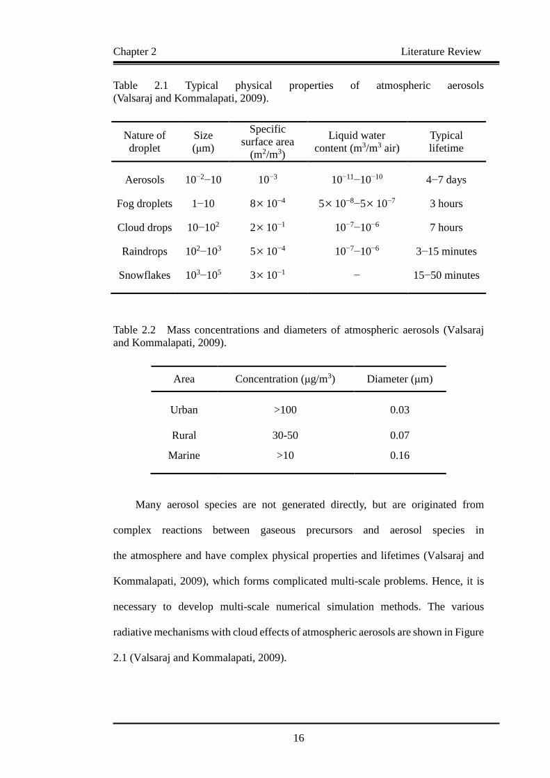
Table 2.1 Typical physical properties of atmospheric aerosols
(Valsaraj and Kommalapati, 2009).
Nature of
droplet
Size
(μm)
Specific
surface area
(m2/m3)
Liquid water
content (m3/m3 air)
Typical
lifetime
Aerosols 10−2−10 10−3 10−11−10−10 4−7 days
Fog droplets 1−10 8 10−4 5 10−8−5 10−7 3 hours
Cloud drops 10−102 2 10−1 10−7−10−6 7 hours
Raindrops 102−103 5 10−4 10−7−10−6 3−15 minutes
Snowflakes 103−105 3 10−1 − 15−50 minutes
Table 2.2 Mass concentrations and diameters of atmospheric aerosols (Valsaraj
and Kommalapati, 2009).
Area Concentration (μg/m3) Diameter (μm)
Urban >100 0.03
Rural 30-50 0.07
Marine >10 0.16
Many aerosol species are not generated directly, but are originated from
complex reactions between gaseous precursors and aerosol species in
the atmosphere and have complex physical properties and lifetimes (Valsaraj and
Kommalapati, 2009), which forms complicated multi-scale problems. Hence, it is
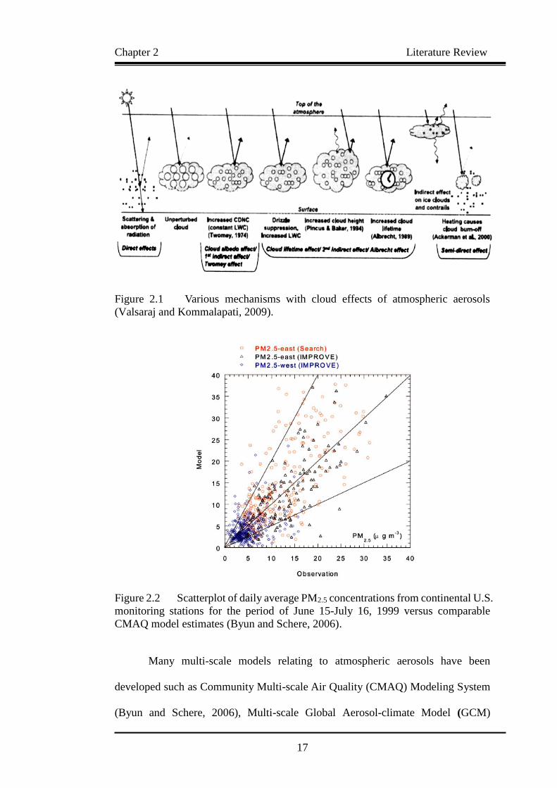
necessary to develop multi-scale numerical simulation methods. The various
radiative mechanisms with cloud effects of atmospheric aerosols are shown in Figure
2.1 (Valsaraj and Kommalapati, 2009).
Chapter 2 Literature Review
17
Figure 2.1 Various mechanisms with cloud effects of atmospheric aerosols
(Valsaraj and Kommalapati, 2009).
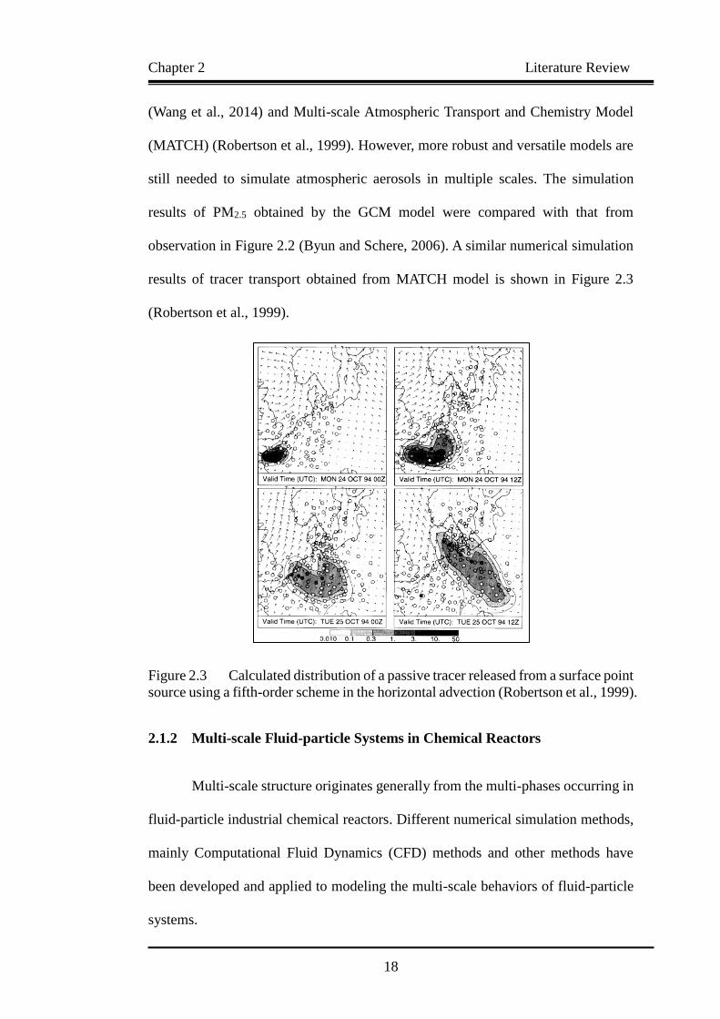
Figure 2.2 Scatterplot of daily average PM2.5 concentrations from continental U.S.
monitoring stations for the period of June 15-July 16, 1999 versus comparable
CMAQ model estimates (Byun and Schere, 2006).
Many multi-scale models relating to atmospheric aerosols have been
developed such as Community Multi-scale Air Quality (CMAQ) Modeling System
(Byun and Schere, 2006), Multi-scale Global Aerosol-climate Model (GCM)
Chapter 2 Literature Review
18
(Wang et al., 2014) and Multi-scale Atmospheric Transport and Chemistry Model
(MATCH) (Robertson et al., 1999). However, more robust and versatile models are
still needed to simulate atmospheric aerosols in multiple scales. The simulation
results of PM2.5 obtained by the GCM model were compared with that from
observation in Figure 2.2 (Byun and Schere, 2006). A similar numerical simulation
results of tracer transport obtained from MATCH model is shown in Figure 2.3
(Robertson et al., 1999).
Figure 2.3 Calculated distribution of a passive tracer released from a surface point
source using a fifth-order scheme in the horizontal advection (Robertson et al., 1999).
2.1.2 Multi-scale Fluid-particle Systems in Chemical Reactors
Multi-scale structure originates generally from the multi-phases occurring in
fluid-particle industrial chemical reactors. Different numerical simulation methods,
mainly Computational Fluid Dynamics (CFD) methods and other methods have
been developed and applied to modeling the multi-scale behaviors of fluid-particle
systems.
Chapter 2 Literature Review
19
Fluidized Bed Reactor
Computational fluid dynamics (CFD) method is often used for the modeling
of multi-scale reaction inside a fluidized bed reactor (FBR) (Zhuang et al., 2014;
Wang et al., 2014; Deen and Kuipers, 2014; Klimanek et al., 2015; Lu et al., 2016).
CFD approaches for the simulation of gas-solid flows in FBRs can be divided into
two categories: Eulerian-Lagrangian and constant Eulerian–Eulerian methods
(Zhuang et al., 2014). Compared with the Eulerian–Lagrangian method, in which
the movement of particles is tracked individually, the Eulerian–Eulerian method
treats particulate phase as a continuous phase (Zhuang et al., 2014).
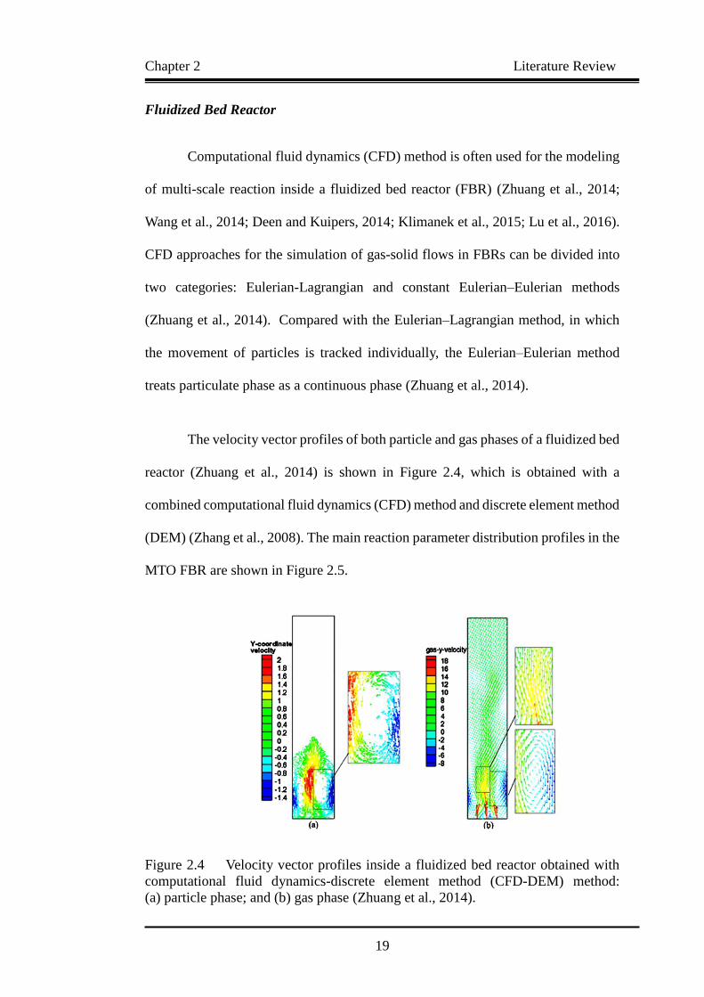
The velocity vector profiles of both particle and gas phases of a fluidized bed
reactor (Zhuang et al., 2014) is shown in Figure 2.4, which is obtained with a
combined computational fluid dynamics (CFD) method and discrete element method
(DEM) (Zhang et al., 2008). The main reaction parameter distribution profiles in the
MTO FBR are shown in Figure 2.5.
Figure 2.4 Velocity vector profiles inside a fluidized bed reactor obtained with
computational fluid dynamics-discrete element method (CFD-DEM) method:
(a) particle phase; and (b) gas phase (Zhuang et al., 2014).

Chapter 2 Literature Review
20
Figure 2.5 Main reaction parameter distribution profiles in the methanol to
olefins (MTO) fluidized bed reactor (FBR) at t = 0.052 s: (a) gas-phase temperature;
(b) particle temperature; (c) coke content; (d) ethane mole concentration; (e) propene
mole concentration; and (f) butene mole concentration; space (velocity= 2.8 m/s,
inlet feed temperature= 723K, feed ratio of water to methanol= 0 (Zhuang et al., 2014).
Fixed Bed Reactor
Fluid flow through fixed bed of spheres is often accompanied by complex
phenomena such as heat and mass transfer (Rong et al., 2014). Methods such as CFD
method and DEM method together with stochastic methods such as Lattice
Boltzmann Method (LBM) (Rong et al., 2014; Asensio et al., 2014;
Mahmoudi et al., 2014; Brumby et al., 2015; Kruggel-Emden et al., 2016) are often
used to simulate multi-scale particle-fluid systems in a fixed bed reactor.
Chapter 2 Literature Review
21
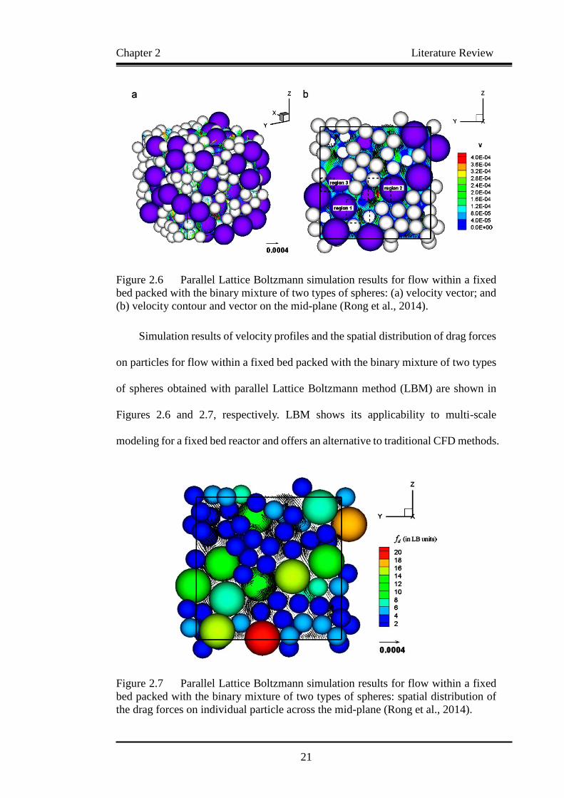
Figure 2.6 Parallel Lattice Boltzmann simulation results for flow within a fixed
bed packed with the binary mixture of two types of spheres: (a) velocity vector; and
(b) velocity contour and vector on the mid-plane (Rong et al., 2014).
Simulation results of velocity profiles and the spatial distribution of drag forces
on particles for flow within a fixed bed packed with the binary mixture of two types
of spheres obtained with parallel Lattice Boltzmann method (LBM) are shown in
Figures 2.6 and 2.7, respectively. LBM shows its applicability to multi-scale
modeling for a fixed bed reactor and offers an alternative to traditional CFD methods.
Figure 2.7 Parallel Lattice Boltzmann simulation results for flow within a fixed
bed packed with the binary mixture of two types of spheres: spatial distribution of
the drag forces on individual particle across the mid-plane (Rong et al., 2014).
Chapter 2 Literature Review
22
2.1.3 Multi-scale Flows and Particle Issues
Another important application of multi-scale particle-fluid systems is the
study of multi-scale flows (Nie et al., 2004; Koumoutsakos, 2005; Bergdorf and
Koumoutsakos, 2006; Oñate et al., 2014; Zhang et al., 2014; He et al., 2014;
Giannakopoulos et al., 2014; Li et al., 2015; Lee and Engquist, 2016). Multi-scale
flow simulations using particles is a widely used method and considered to be an
efficient one.
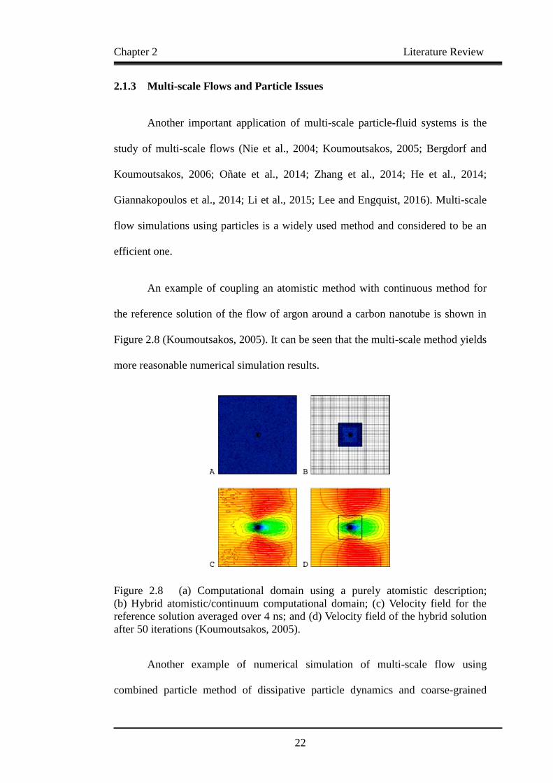
An example of coupling an atomistic method with continuous method for
the reference solution of the flow of argon around a carbon nanotube is shown in
Figure 2.8 (Koumoutsakos, 2005). It can be seen that the multi-scale method yields
more reasonable numerical simulation results.
Figure 2.8 (a) Computational domain using a purely atomistic description;
(b) Hybrid atomistic/continuum computational domain; (c) Velocity field for the
reference solution averaged over 4 ns; and (d) Velocity field of the hybrid solution
after 50 iterations (Koumoutsakos, 2005).
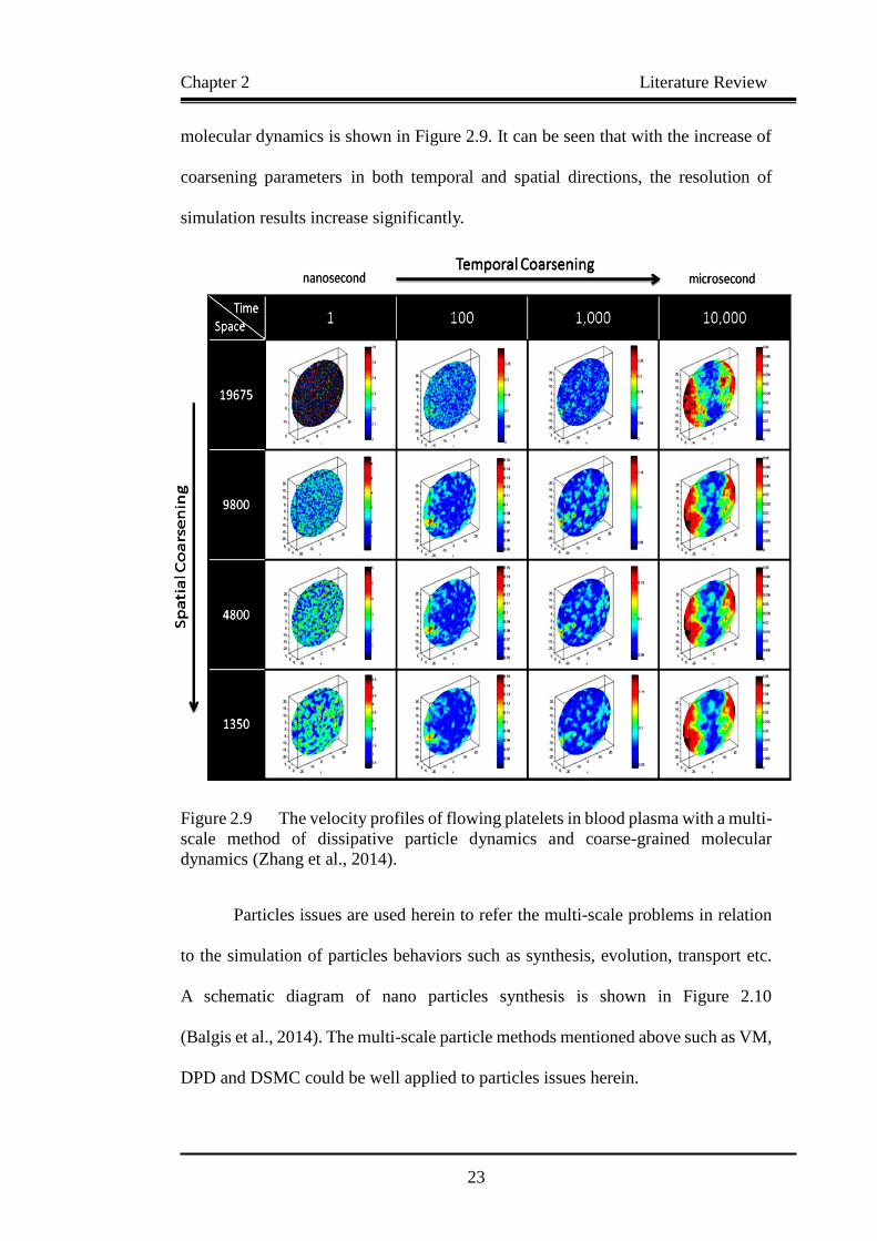
Another example of numerical simulation of multi-scale flow using
combined particle method of dissipative particle dynamics and coarse-grained
Chapter 2 Literature Review
23
molecular dynamics is shown in Figure 2.9. It can be seen that with the increase of
coarsening parameters in both temporal and spatial directions, the resolution of
simulation results increase significantly.
Figure 2.9 The velocity profiles of flowing platelets in blood plasma with a multi-
scale method of dissipative particle dynamics and coarse-grained molecular
dynamics (Zhang et al., 2014).
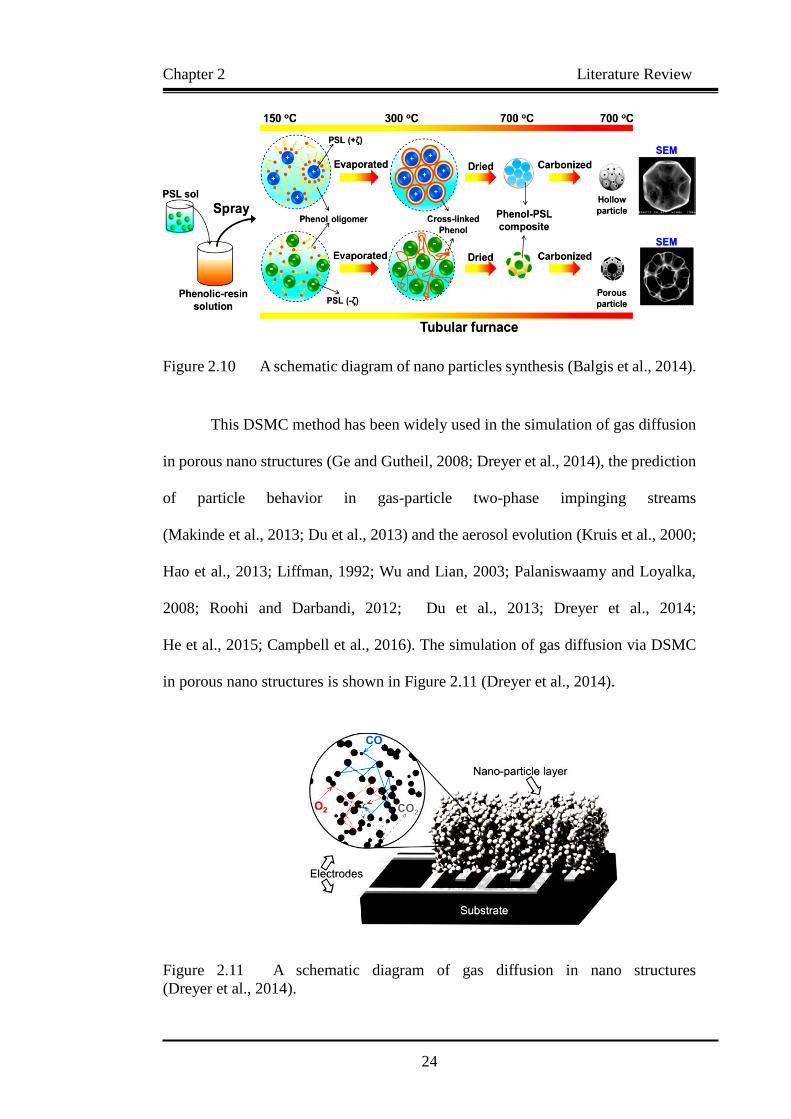
Particles issues are used herein to refer the multi-scale problems in relation
to the simulation of particles behaviors such as synthesis, evolution, transport etc.
A schematic diagram of nano particles synthesis is shown in Figure 2.10
(Balgis et al., 2014). The multi-scale particle methods mentioned above such as VM,
DPD and DSMC could be well applied to particles issues herein.
Chapter 2 Literature Review
24
Figure 2.10 A schematic diagram of nano particles synthesis (Balgis et al., 2014).
This DSMC method has been widely used in the simulation of gas diffusion
in porous nano structures (Ge and Gutheil, 2008; Dreyer et al., 2014), the prediction
of particle behavior in gas-particle two-phase impinging streams
(Makinde et al., 2013; Du et al., 2013) and the aerosol evolution (Kruis et al., 2000;
Hao et al., 2013; Liffman, 1992; Wu and Lian, 2003; Palaniswaamy and Loyalka,
2008; Roohi and Darbandi, 2012; Du et al., 2013; Dreyer et al., 2014;
He et al., 2015; Campbell et al., 2016). The simulation of gas diffusion via DSMC
in porous nano structures is shown in Figure 2.11 (Dreyer et al., 2014).
Figure 2.11 A schematic diagram of gas diffusion in nano structures
(Dreyer et al., 2014).

Chapter 2 Literature Review
25
2.2 Experimental investigation of aerosol dynamics
The experimental investigation of aerosol dynamics mainly includes
the collection, examination and characterization of aerosol particles, which will be
introduced respectively in the following sections.
2.2.1 Collection of Aerosol Particles
The collection of aerosol particles can be conducted in a batchwise way or
continually such as continuous online sampling. Some online sampling methods
have been developed particularly for the online sampling of aerosol particles
originating from combustion (Chen et al., 1998; Maricq et al., 2003;
Zhao et al., 2003; Jiménez and Ballester, 2005; Laitinen et al., 2010;
Hess et al., 2016) and vehicle emissions (Chan et al., 2004; Alvarez et al., 2008;
Ježek et al., 2015). Considering the impact of external electrostatic field, the
collection of aerosol particles can be conducted in the presence of external
electrostatic fields (Intra et al., 2014) or in the absence of them (Smith and Phillips,
1975). Figure 2.12 shows a typical example of online sampling system (Zhao et al.,
2003).
Figure 2.12 A schematic diagram of an online sampling system
(Zhao et al., 2003).

Chapter 2 Literature Review
26
2.2.2 Examination and Characterization of Aerosol Particles
Chromatography and mass spectrometry have been widely used for
the analysis of small scale of aerosol particles after proper pretreatment.
Nuclear magnetic resonance and Raman spectroscopy have also been used to
examine more microscopic properties of certain aerosol particles such as soot.
Laser desorption has been connected to mass spectrometry (Bouvier et al., 2007;
Öktem et al., 2005; Laskin et al., 2010; Ozawa et al., 2016) to measure the relative
abundance of organic components on soot particles.
For a larger scale examination of aerosol particles, optical methods such as
transmission electron microscopy (TEM) and scanning electron microscopy (SEM)
can be used. For a sample with large number of aerosol particles, light scattering and
absorption measurements can be used to estimate particle diameters and obtain
a multi-modal PSD (Erickson et al., 1964).
2.3 Numerical Methods for the Simulation of Aerosol Dynamics
Various numerical methods have been developed to solve Equation (1-1),
the population balance equation (PBE) governing the evolution of particle number
density as a function of particle size and time. The main numerical methods for
aerosol dynamics include sectional methods (Jeong and Choi, 2001;
Mitrakos et al., 2007; Agarwal and Girshick, 2012), method of moments
(Lin and Chen, 2013; Yu et al., 2008; Park et al., 2013; Chen et al., 2014;
Yu and Chan, 2015; Pollack et al., 2016) as well as stochastic method
(Zhao et al., 2009; Zhao et al., 2012; Wei, 2013, Zhou et al., 2014; Liu et al., 2015;
Liu and Chan, 2016 and 2017).

Chapter 2 Literature Review
27
2.3.1 Sectional Method
Sectional methods can be classified into fixed sectional methods and moving
sectional methods. The fixed sectional methods first proposed by Gelbard and
Seinfeld (1980) use a grid placed on the particle type or state space with an a priori
assumption of the shape of PSD in every section bin or grid cell (Patterson, 2007).
The moving sectional methods proposed by Kumar et al. (1997) adjust
the boundaries of section bins to account for the particle size changes due to aerosol
dynamic processes.
Figure 2.13 Comparison between sectional and analytical methods: normalized
number and volume concentrations under constant coagulation and linear
condensation (Mitrakos et al., 2007).
Figure 2.13 shows the evolution of the normalized particle number and
volume concentrations of the aerosols as a function of the dimensionless time
(Mitrakos et al., 2007). The decrease of normalized particle number due to
coagulation as well as the increase of particle volume due to condensation are well
Chapter 2 Literature Review
28
captured by numerical simulation compared with the analytical solution
(Mitrakos et al., 2007) as is shown in Figure 2.18.
2.3.2 Method of Moments
The main advantage of methods of moments in the simulation for aerosol
dynamics is the relatively low computational cost (i.e., computational time,
computer memory, etc.) as a small number of additional equations i.e.,
the moments equations of the PSD are to be solved while the main disadvantage is
the requirement of initial PSD in order to obtain the closure of the transport equations
(Mitrakos et al., 2007).
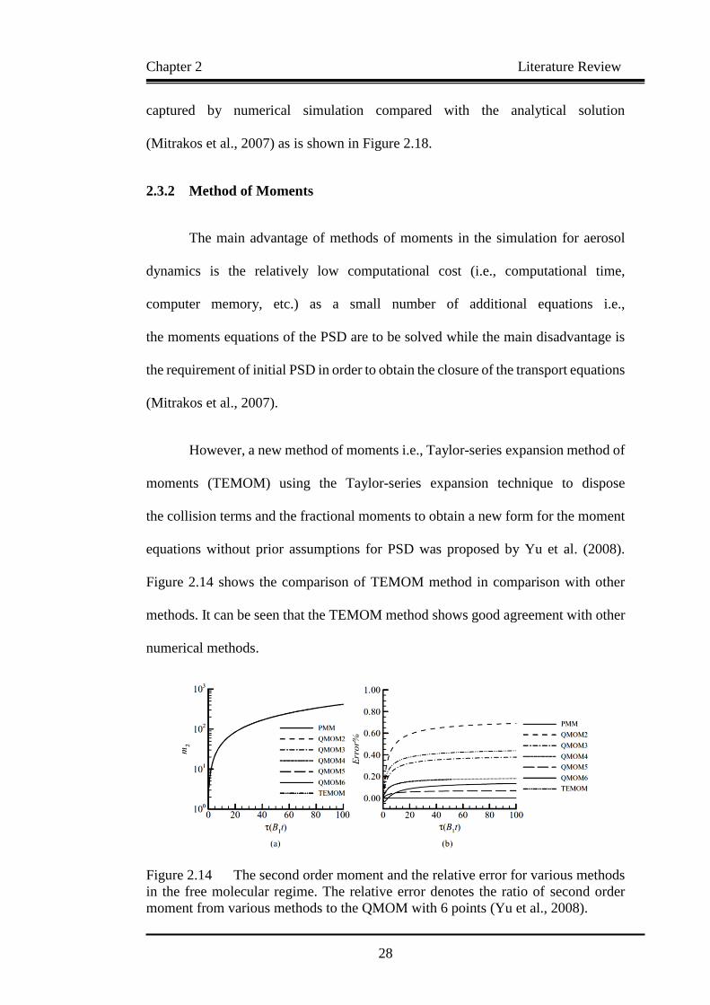
However, a new method of moments i.e., Taylor-series expansion method of
moments (TEMOM) using the Taylor-series expansion technique to dispose
the collision terms and the fractional moments to obtain a new form for the moment
equations without prior assumptions for PSD was proposed by Yu et al. (2008).
Figure 2.14 shows the comparison of TEMOM method in comparison with other
methods. It can be seen that the TEMOM method shows good agreement with other
numerical methods.
Figure 2.14 The second order moment and the relative error for various methods
in the free molecular regime. The relative error denotes the ratio of second order
moment from various methods to the QMOM with 6 points (Yu et al., 2008).
Chapter 2 Literature Review
29
2.3.3 Stochastic Method
The direct simulation Monte Carlo (DSMC) method was first proposed by
Bird (1994). The basic idea of DSMC is to use a set of numerical particles to
represent the real physical particles. However, only the particle properties of interest
such as momentum and mass are tracked. The random generation of collisions based
on prescribed probability laws is justified by the molecular chaos
(Baxter and Olafsen, 2007) in homogeneous grid cells. A review of the DSMC
methods and some practical application in solving the Boltzmann equation can be
found in Oran et al. (1998). Figure 2.15 shows the regimes of validity of DSMC and
other methods.
Figure 2.15 Regimes of validity of molecular dynamics, direct simulation Monte
Carlo, and Navier-Stokes, as a function of the characteristic length scale and mean
molecular spacing of a system (Oran et al., 1998).

Chapter 2 Literature Review
30
2.4 Direct Simulation Monte Carlo Method
2.4.1 Overview
The direct simulation Monte Carlo Method (DSMC) proposed by Bird (1994)
uses numerical particles to represent a large number of physical molecules or atoms,
which is a well-established method in the simulation of non-equilibrium gas flows.
The DSMC method models gas at the microscopic level and the gas physics is thus
captured through the motion of particles and collisional interaction between them.
The DSMC method is statistical in nature because of the probabilistical and
phenomenological treatment of physical process like collision in order to reproduce
the macroscopic behavior of particles (Wu and Lian, 2003).
The primary advantage of the DSMC method is that it can capture
the non-equilibrium effects which may occur in aerosol dynamics due to the
relatively high Knudsen number (denoted by Kn), which is defined as the ratio of
the mean free path length of the gas to the characteristic length of interest
(the aerosol size). As aerosol particles are of micro- or nano- level, it generally yields
a Knudsen number falling into the transitional regime (10−3<Kn<10). By tracking
representative particles through space and considering collisions between particles,
the DSMC method can directly simulate the physics of aerosol dynamics.
Mathematically, the Boltzmann equation can be derived by following DSMC
procedures.

Chapter 2 Literature Review
31
2.4.2 Particle Representation
Particles in a DSMC simulation are set to represent a large number of real
gas particles (Rieffel, 1999). Each simulation particle can be considered as
a representative sample from the physical particulate system or as an average of
the real particles according to the mean field theory. Particles are generally
considered to be point particles or spheres with associated properties such as species,
velocity and internal energy. The actual shape of molecules and the associated
three-dimensional force fields are generally neglected for computational simplicity.
Collisions between particles are treated probabilistically using corresponding
models. The common collisional models include hard sphere (HS) model,
variable hard sphere (VHS) model, generalized hard sphere (GHS) model,
variable soft sphere (VSS) model and some other models (Bird, 1994).
The operation of collision and sampling steps requires particles to be grouped
into the cells of certain computational cells. The particles thus need to be sorted
properly into corresponding groups. Collisions between the particles make it
possible for the properties of gas to be transmitted through bulk flow.
The exact calculation of collision kinematics involves many physical properties of
particles such as the particles’ trajectories, angles of incidence and impact parameter
which is much costly. So collisions are calculated statistically between particles
residing in the same computational cell. After being grouped into certain cells,
a list of possible collision pairs is thus formed. A common method to decide whether
collision happens is the acceptance-rejection method. Once the collision model and
sampling scheme are determined, the collision probability is the function of
the relative velocities, collision cross section and the number density of particles in

Chapter 2 Literature Review
32
the cells. However, the collision probability is also related to the time step previously
set and the particle weight, which will be introduced in Chapter 4.
A pair of particles is accepted for collision if the collision probability
mentioned above is greater than a random number. The average collision rate is
equal to that given by the kinetic theory, which guarantees the reliability of
the statistical collision models. Several schemes had been proposed to be the criteria
of collision occurrence such as the time counter and no time counter methods by
Bird (1994).
Once a pair is selected for collision, momentum and energy are exchanged,
the actual trajectories and dynamics of the particles are not taken into account in
determining the collision mechanics. This is because the distribution function based
on mean field theory is applied to the whole cell being considered.
Instead, the scattering angle and degree of inelasticity can be selected statistically in
order to generate post collision properties. Energy and momentum are obviously
conserved in each collision.
2.4.3 Algorithm and Numerical Simulation Parameters
The DSMC method assumes that particle movement can be decoupled from
collisional behavior in a small time step. Particles then move along straight line paths
with discrete changes in velocity and energy caused by collisions. In order to
accomplish this, the simulation is broken up into time steps for the magnitude of
which are small compared to the average time between collisions (He and Zhao,
2016). In this small interval of time, these two processes can realistically be treated
as independent.

Chapter 2 Literature Review
33
A complete DSMC simulation consists of a series of discrete time steps or
iterations. During each iteration, particles are moved and collisional pair is chosen
and computed. The typical algorithm of a single iteration in the DSMC method is as
follows:
Step 1: Move particles;
Step 2: Perform boundary interaction;
Step 3: Sort particles into cells;
Step 4: Select collision pairs;
Step 5: Compute collision mechanics; and
Step 6: Sample macroscopic properties of interest.
The first five operations are performed in each iteration. The sixth step is
performed only when flow properties are desired. In the present study, the common
numerical simulation parameters include particle weight, WP, time step and grid cell
size.
Particle Weight
Each simulation particle in DSMC simulation represents a large number of
real particles (Guan et al., 2014). The ratio of the number of numerical particles,
NS to the number of physical particles, NR (or real particles) is defined as the particle
weight.
WP = NR/NS (2-1)
The smaller the particle weight, the larger number of numerical particles and
thus better resolution of the flow physics. However, the larger number of numerical

Chapter 2 Literature Review
34
particles means larger computational cost (i.e., computational time, computer
memory, etc.). So the particle weight is selected to strike a reasonable balance
between resolution of results, and computational cost and efficiency.
In traditional DSMC method, numerical particles are associated with equal
weight regardless of the broad PSD, in which the particle number density in different
particle size ranges may be quite different. The resulting statistical error and limited
particle size spectrum will no doubt restrict the application of the DSMC method
(Zhao et al., 2009). One method to deal with this problem is to introduce variable
particle weights. For example, varying weights in the radial direction are used in the
axisymmetric flows. In this case, the particle weight is increased in cells away from
the axis to counteract the increasing volumes of these cells. Moreover, different
weighting scales can be used to increase resolution in regions of the flow field with
low particle number density or to increase computational efficiency where there is
an excessive number of particles. This is why the stochastic weights are associated
with numerical particles in the present study.
There is a problem of continuity on the interface concerning the usage of
varying weights i.e., cells across the interface are with different weights.
A discontinuity in mass flux across the interface is thus created when a particle
crosses the interface and suddenly represents a different number of real particles.
This discontinuity can be overcome by allowing a probability that the particle is
either cloned when moving into a cell with a lower particle weight or destroyed when
moving into a cell with a higher particle weight. The scheme can be described as
follows:
Chapter 2 Literature Review
35
WPold>WP
new:Pclone= WPold WP
new⁄ 1 (2-2)
WPold<WP
new:Pdestroy = WPold WP
new⁄ (2-3)
where WPold , WP
new , Pdestroy and Pclone represent the particle weights of the old
cell, the particle weight of the new cell, the probability of the particle to be destroyed
and the probability that the particle to be cloned, respectively. The clone-destroy
operation conserves mass flux across the interface when many crossings are
averaged. The stochastically weighted Monte Carlo method will be further described
in Chapter 4.
Time Step
A certain finite number of time steps are used to decouple the movement of
particles from collisions. In order to do this, the time step must be a small fraction
of the mean time between collisions. The exact expression is dependent on
the collision model employed but is in general a function of density and temperature.
For purpose of statistical accuracy, it is also desirable that a particle not remain in
a single cell for a large number of time steps. A high residence time tends to bias
the sampling of macroscopic properties. The time step should then be set at a large
enough value so that the majority of particles moving at the bulk fluid velocity will
cross a given cell in a small number of time steps. Residence time and mean collision
time provide bounds for the selection of a simulation time step.
Grid Cell Size
Grid cells in computational domain is used in DSMC to group particles for
the purposes of calculating collisions and sampling macroscopic properties.
Chapter 2 Literature Review
36
The size of the computational cells is limited by the constraints of physical accuracy
and computational efficiency. As previously mentioned, collisions are calculated
statistically between pairs of particles residing in the same cell. The two particles
participating in a collision may be separated in space by as much as one cell
dimension. In a real gas, two particles will not collide if they are separated by more
than one mean free path. This provides a limit on the size of the computational cell.
Ideally, cell dimensions should be smaller than the local mean free path such as
30 percent of the mean free path at all points as recommended by Bird (1994).
Sampling of Macroscopic Properties
The macroscopic properties can be taken as the average of the local
properties of the molecules consisting of the gas. Density, velocity and temperature
are the zeroth, first and second order moments of the velocity distribution function.
Since the DSMC method directly depicts the distribution function, flow field results
can be determined by sampling particles properties and calculating the moments of
the distribution function of the sample. The computational grid is used to group
particles for the purpose of sampling their properties and calculation is also
conducted in every cell.
Calculation of smooth flow properties requires a large sample size in order
to accurately describe the distribution function as the statistical noise is generally
proportional to the inverse of the square root of the sample size (Darbandi et al.,
2010). One of the methods to reduce the statistical noise is to sample over a number
of iterations to increase the sample size and thus reduce the simulation fluctuations.
In time dependent flows, it is often necessary to perform an ensemble average over
many different simulations to obtain acceptable simulation results.

Chapter 2 Literature Review
37
2.5 Operator Splitting Monte Carlo Method
2.5.1 Overview
Differential equations, including partial differential equations (PDE) and
ordinary differential equations (ODE) have gained a wide range of engineering and
scientific applications in terms of models of various physical phenomena.
These differential equations are becoming increasingly complicated as the models
to be described are becoming more and more complicated, representing increasingly
complicated physical phenomena. It is common that a model contains different terms
(operators) reflecting different physical or chemical processes. Consider the general
dynamic equation (GDE) (Friedlander, 2000) in Equation (2-4),
it contains convection, diffusion, nucleation, growth and coagulation terms.
These different terms reflecting different aspects of the model appear in the same
equation, making it rather difficult to analyze and solve both analytically and
numerically.
∂n
∂t+∇⋅D∇n= [
∂n
∂t] coag+ [
∂n
∂t] grow+ [
∂n
∂t] nucl
where the subscripts coag, grow and nucl represent the processes of coagulation,
surface growth and nucleation, respectively.
Operator splitting based on the idea of divide and conquer is a very efficient
and successful strategy to deal with those complex PDEs (Mclachlan and Quispel,
2002). The idea behind operator splitting is that the overall evolution operator is
written as a sum of evolution operators for each operator (term), that is,
one just splits the model into a set of sub-equations, where each sub-equation is of
(2-4)

Chapter 2 Literature Review
38
a type for which solution to the equation can be found more easily. The overall
numerical method is then formed by picking an appropriate numerical scheme for
each sub-equation and piecing the schemes together by operator splitting
(Holden et al., 2010).
Splitting methods arise when a vector space can be split into a sum of two or
more parts that are each simpler to integrate that the original equation, which are
composed to form the integrator once a splitting is constructed (Mclachlan and
Quispel, 2002). Consider a simple time dependent differential equation, dx/dt = X(x)
with x within phase, M where X is a vector field on phase M, the splitting methods
involve the following three important steps (Mclachlan and Quispel, 2002):
1. Choosing a set of vector fields, Xi such that X = ∑ Xi ;
2. Integrating either exactly or approximately for each Xi ; and
3. Combining these solutions to yield an integrator for X.
Consider the following Cauchy problem, the splitting method can be
formulated as follows:
dU
dt+A(U)=0, U(0)=U0
where A is some unspecified operator. Consider the following solution: A = A1+A2
is assumed and then one can solve the sub-problems more easily (Holden et al.,
2010).
dU
dt+Aj(U) = 0, U(0) = U0, j=1, 2, ...
(2-5)
(2-6)

Chapter 2 Literature Review
39
with formal solutions as follows:
Uj(t) = e tAjU0, j=1, 2, … (2-7)
In its simplest form, the operator splitting reads as follows: let tn = n∙∆t
(∆t is small and positive) (Holden et al., 2010). Approximately, it is written as:
U(tn+1) = e∆tA1e∆tA2U(tn) (2-8)
For commuting operators, e tA1e tA2 = e tA , the method would be exact.
Holden et al. (2010) suggested that an operator splitting may be considered as
the method of choice if the operators are weakly coupled, that is, if the interaction
of the different physical phenomena has a long time scale, an operator-splitting
scheme will be efficient over a wide range of sizes for the splitting steps.
Furthermore, it may be the only feasible method for higher dimensional problems.
On the other hand, if the operators interact significantly over a short time scale,
the operator splitting may be subject to severe restrictions on the splitting step.
For nonlinear operators, Holden et al. (2010) pointed out that interaction
between elementary operators is often nonlinear, and splitting them into separate
steps may result in large and unwanted errors. Operator splitting has been applied
widely to many areas such as celestial mechanics, molecular dynamics,
accelerator physics and biology diffusion-reaction system.
2.5.2 Operator Splitting Schemes
The Equation (2-4) includes various aerosol dynamic processes. Operator
splitting is very efficient in solving such evolution equation. In the implementation
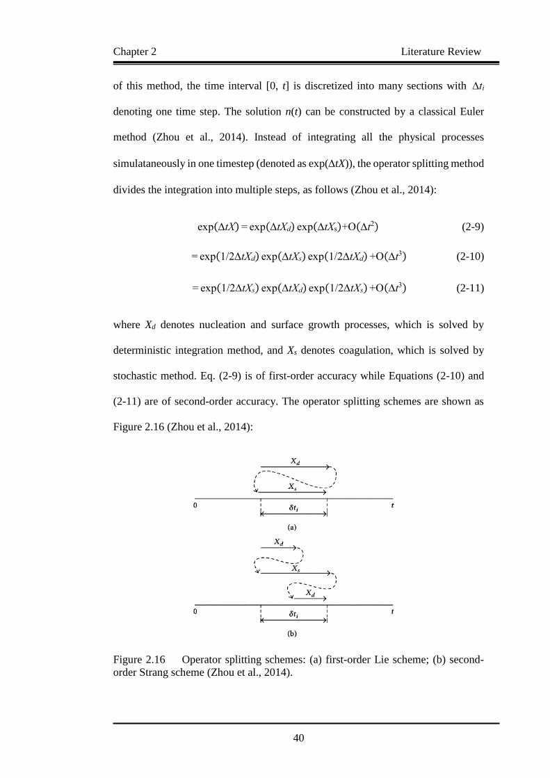
Chapter 2 Literature Review
40
of this method, the time interval [0, t] is discretized into many sections with ∆ti
denoting one time step. The solution n(t) can be constructed by a classical Euler
method (Zhou et al., 2014). Instead of integrating all the physical processes
simulataneously in one timestep (denoted as exp(tX)), the operator splitting method
divides the integration into multiple steps, as follows (Zhou et al., 2014):
exp(tX) = exp(tXd) exp(tXs)+O(t2) (2-9)
= exp(1/2tXd) exp(tXs) exp(1/2tXd) +O(t3) (2-10)
= exp(1/2tXs) exp(tXd) exp(1/2tXs) +O(t3) (2-11)
where Xd denotes nucleation and surface growth processes, which is solved by
deterministic integration method, and Xs denotes coagulation, which is solved by
stochastic method. Eq. (2-9) is of first-order accuracy while Equations (2-10) and
(2-11) are of second-order accuracy. The operator splitting schemes are shown as
Figure 2.16 (Zhou et al., 2014):
Figure 2.16 Operator splitting schemes: (a) first-order Lie scheme; (b) second-
order Strang scheme (Zhou et al., 2014).
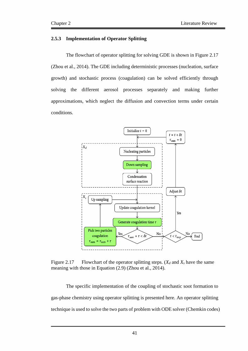
Chapter 2 Literature Review
41
2.5.3 Implementation of Operator Splitting
The flowchart of operator splitting for solving GDE is shown in Figure 2.17
(Zhou et al., 2014). The GDE including deterministic processes (nucleation, surface
growth) and stochastic process (coagulation) can be solved efficiently through
solving the different aerosol processes separately and making further
approximations, which neglect the diffusion and convection terms under certain
conditions.
Figure 2.17 Flowchart of the operator splitting steps. (Xd and Xs have the same
meaning with those in Equation (2.9) (Zhou et al., 2014).
The specific implementation of the coupling of stochastic soot formation to
gas-phase chemistry using operator splitting is presented here. An operator splitting
technique is used to solve the two parts of problem with ODE solver (Chemkin codes)

Chapter 2 Literature Review
42
and Monte Carlo (MC) solver, respectively (Celnik et al., 2007). The governing
equations are as follows:
dfi
dt=Wd (x1, x2, x3)+Ws (x1, x2, x3)
where fi is parameter of interest, Wd and Ws are deterministic processes and stochastic
processes, respectively. Then Equation (2-12) can be solved as follows:
ODE solver:
df'
dt=Wd (x'1, x'2, x'3), f'i (t0)= fi (t0), t0<t<t0+h/2
MC solver:
df''
dt=Ws(x''1, x''2, x''3), f''i (t0) = f'i (t0+h/2), t0<t<t1
ODE solver:
f''' i (t0) = f''i (t0+h/2), t0+h/2<t<t1
Finally, the computed values are assigned at the step endpoint.
f (t1)= f''i (t1) (2-16)
2.6 Weighted Monte Carlo Methods
2.6.1 Overview
In most of the conventional Monte Carlo methods, each simulation particle
is associated with the uniform number of particles. The accuracy of the numerical
(2-12)
(2-13)
(2-14)
(2-15)
Chapter 2 Literature Review
43
simulation thus depends on the number of numerical particles used
(Zhao et al., 2005). This decreases the applicability of Monte Carlo method alone to
the spatially resolved gas simulations, by which regions with few physical particles
cannot be modeled accurately. In most Monte Carlo methods, a subsystem out of a
total system is simulated. In general, numerical particles are equally weighted with
a value of V/Vs, where V and Vs are the volume of the whole system and those of the
subsystem, respectively (Zhao et al., 2009). Consider a system with a total particle
number concentration of 1×10¹⁰ m−3 contains 1×10⁴ numerical particles, so each
simulation particle represents 106 real particles and the weight can be defined as the
ratio of the number of real particles to that of the numerical particles, which is 1×10⁶.
It is obvious by this definition that every numerical particle represents the same
number of real particles. However, there is insufficient number of particles at the
edges of the size spectrum, which makes it impossible to accurately capture the
particle size distribution in this area using Monte Carlo method alone (Zhao et al.,
2010). This becomes especially significant when the particle size distribution
function is displayed in the usual logarithmic representation (Zhao et al., 2009).
2.6.2 Different Weighting Numerical Particles Schemes
The concept of weighting numerical particles is widely used as described
above to overcome the conflict between large number of real particles and limited
computational capacity (Zhao et al., 2009). A stochastically weighted particle
method (SWPM) was thus introduced by Rjasanow and Wagner (1996) to deal with
this problem of simulation accuracy, in which each simulation particle was
associated with a stochastic weight, i.e., the number of real particles that they are
associated with. With this SWPM, a larger number of numerical particles with

Chapter 2 Literature Review
44
smaller stochastic weights can be applied in regions with lower density than was
the case with basic DSMC. A similar problem could occur in zero-dimensional
particle coagulation problems, in which the resolution of the upper end of the PSD
in the DSMC simulation can be quite low because of the small number of numerical
particles over there and thus causes a great statistical error. Different weighted
schemes are proposed to deal with these problems (Eibeck and Wagner, 2001;
Zhao et al., 2009; DeVille et al., 2011; Liu and Chan, 2017). The particle-weighting
scheme proposed by Eibeck and Wagner (2001) can be further generalized into mass
flow algorithm (MFA) by the proper derivations.
2.7 CFD-Population Balance Modelling of Aerosol Dynamics
In zero-dimensional simulation of aerosol dynamics, the spatially
homogeneous flow field is assumed, neglecting the spatial inhomogeneity and
coupling between the dispersed phase (aerosol particles) and continuous phase
(fluid). However, the spatial inhomogeneity and inter-phase interaction become
significant in most scientific and engineering applications. In order to obtain more
accurate simulation results, a better control over particle size distribution and design
of the equipment related to particulate processes, the population balance modelling
(PBM) coupling with CFD to realize the multi-dimensional simulation of aerosol
dynamics is required (Zhao and Zheng, 2013). CFD-PBM methods for aerosol
dynamics are thus formulated to account for the spatial inhomogeneity and
inter-phase interaction of aerosol dynamics in many practical applications
(Kruis et al., 2012; Zhao and Zheng, 2013; Zhou and Chan, 2014; Zhou and He,
2014; Akridis and Rigpoulos, 2015; Amokrane et al., 2016; Liu and Chan, 2016).
Taking into the consideration on inter-phase interaction between the particulate
Chapter 2 Literature Review
45
phase and fluid phase, the coupling between the PBM and CFD codes can be divided
into one-way coupling, two-way coupling or even four-way coupling. In one-way
coupling, only the influence of fluid phase on particulate phase is considered (Zucca
et al., 2007; Kruis et al., 2012; He and Zhao, 2016). In two-way coupling, the
interaction between particulate phase and fluid phase are taken into account while
the inter-particle interaction is neglected (Boivin et al., 2000; Pialat et al., 2006;
Zhang and You, 2015). However, due the complexity of implementation, four-way
coupling between the PBM and CFD codes is rarely reported (Zhao and Zheng, 2013;
He and Zhao, 2016).
According to the simulation methodology for dispersed phase i.e.,
aerosol particles, the CFD-PBM methods can be classified into Eulerian-Eulerian
models and Eulerian-Lagrangian models. In the Eulerian-Eulerian models,
the deterministic methods such as method of moments (Settumba and Garrick, 2004;
Balthasar and Frenklach, 2005; Zucca et al., 2006; Chen et al., 2011; Basavarajappa
and Miskovic, 2016) and sectional methods (Jeong and Choi, 2003; Wen et al., 2005;
Nere and Ramkrishna, 2006; Mitrakos et al., 2007; Agarwal and Girshick, 2012) are
used to directly solve the PBE (i.e., Equation (1-1)) of aerosol particles.
Meanwhile, in the Eulerian-Lagrangian models, stochastic methods such as Monte
Carlo methods (Kruis et al., 2012; Zhao and Zheng, 2013; Fede et al., 2015;
He et al., 2015; Consalvi and Nmira, 2016) are used to simulate the evolution of
PBE of aerosol particles. The deterministic methods, which solve the PBE based on
the Eulerian reference frame, are easier and more straightforward to couple with
the Eulerian models of hydrodynamics of fluid phase than stochastic methods.
However, the deterministic PBM methods for aerosol dynamics exhibit relatively

Chapter 2 Literature Review
46
lower resolution on particle dynamics and are unable to consider polydispersity of
particles. Besides these, deterministic PBM methods are unable to capture
the history information and are at disadvantage to get more than two physical
properties of particles (Zhao and Zheng, 2013). Stochastic PBM methods i.e.,
Monte Carlo PBM methods avoid all these disadvantages of the deterministic PBM
methods except for a relatively higher computational cost (i.e., computational time,
computer memory etc.), which can be overcome with the high-speed development
of computer hardware and parallel computing techniques (Zhou et al., 2014;
Xu et al., 2015).
2.8 Transported PDF Methods for Turbulent Reactive Flows
2.8.1 Overview
Transported PDF methods have been developed to overcome the closure
problems due to interaction between turbulence and particle evolution in turbulent
reactive flows by many researchers (Pope, 1981; Pope, 1985; Valino, 1998;
Sabel’nikov and Soulard, 2005; Meyer, 2010; Haworth, 2010; Pope and Tirunagari,
2014; Consalvi and Nmira, 2016). No additional assumptions are made for closure
of PSD and particle number density distribution via the transported PDF methods.
The work of Di Veroli and Rigopoulos (2010) was the first paper to develop
a Lagrangian Monte Carlo method for solving the PDF of the PSD in a reactive
precipitation problem and this method was used on an aerosol condensation problem
in Di Veroli and Rigopoulos (2011). The concept was applied to LES in
Pesmazoglou et al. (2014) and to deal with the aggregation in Pesmazoglou et al.
(2016). The theory underlying transported PDF methods was provided in detail by
Chapter 2 Literature Review
47
Fox (2003). Additionally, the complex and arbitrary kernels of aerosol dynamics are
allowed since no closure is required for the PBE.
Transported PDF methods can be divided into two categories i.e.,
Eulerian PDF methods (Pope, 1981; Pope, 1985) and Lagrangian PDF methods
(Pope, 1994; Jenny et al., 2001), respectively. Improvements of the PDF methods
such as Eulerian field methods (Valiño, 1998; Sabel’nikov and Soulard, 2005;
Jaishree and Haworth, 2012; Consalvi and Nmira, 2016) have also been proposed.,
The transported PDF is approximated by an ensemble of particles that remain fixed
on the nodes of a CFD grid for the Eulerian particle method, but is approximated by
an ensemble of particles that move along a CFD grid in accordance with the flow
field obtained by the CFD codes for the Lagrangian particle method
(Rigopoulos, 2007). Eulerian field method has been proposed in recent years,
where the transported PDF is approximated by an ensemble of stochastic fields
obtained via the CFD codes (Rigopoulos, 2007). Compared to Lagrangian particle
methods, the Eulerian field methods are more compatible with conventional CFD
codes and is thus possible to have higher computational efficiency
(Jaishree and Haworth, 2012). The advantages and disadvantages of different
transported PDF methods are available in the comparison between Eulerian and
Lagrangian Monte Carlo PDF methods (Möbus et al., 2001; Zhang and Chen, 2007;
Haworth, 2010). A modelled composition PDF transport equation is given in
Equation (2-17) (Pope, 1985):
∂ρfϕ
∂t+
∂ρui fϕ
∂xi+
∂ρSαfϕ
∂ψα=
+∂
∂xi[ΓTϕ
∂(ρfϕ <ρ>⁄ )
∂xi]
∂[Sα(ψ)ρfϕ]
∂ψα (2-17)
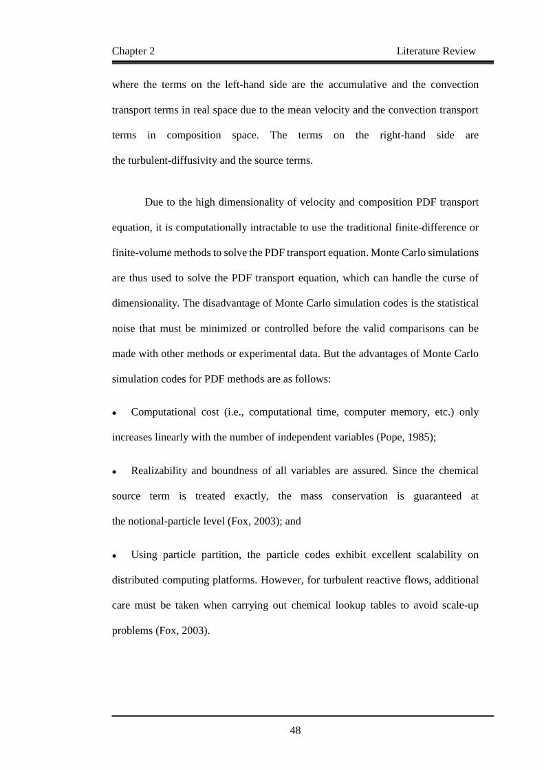
Chapter 2 Literature Review
48
where the terms on the left-hand side are the accumulative and the convection
transport terms in real space due to the mean velocity and the convection transport
terms in composition space. The terms on the right-hand side are
the turbulent-diffusivity and the source terms.
Due to the high dimensionality of velocity and composition PDF transport
equation, it is computationally intractable to use the traditional finite-difference or
finite-volume methods to solve the PDF transport equation. Monte Carlo simulations
are thus used to solve the PDF transport equation, which can handle the curse of
dimensionality. The disadvantage of Monte Carlo simulation codes is the statistical
noise that must be minimized or controlled before the valid comparisons can be
made with other methods or experimental data. But the advantages of Monte Carlo
simulation codes for PDF methods are as follows:
Computational cost (i.e., computational time, computer memory, etc.) only
increases linearly with the number of independent variables (Pope, 1985);
Realizability and boundness of all variables are assured. Since the chemical
source term is treated exactly, the mass conservation is guaranteed at
the notional-particle level (Fox, 2003); and
Using particle partition, the particle codes exhibit excellent scalability on
distributed computing platforms. However, for turbulent reactive flows, additional
care must be taken when carrying out chemical lookup tables to avoid scale-up
problems (Fox, 2003).
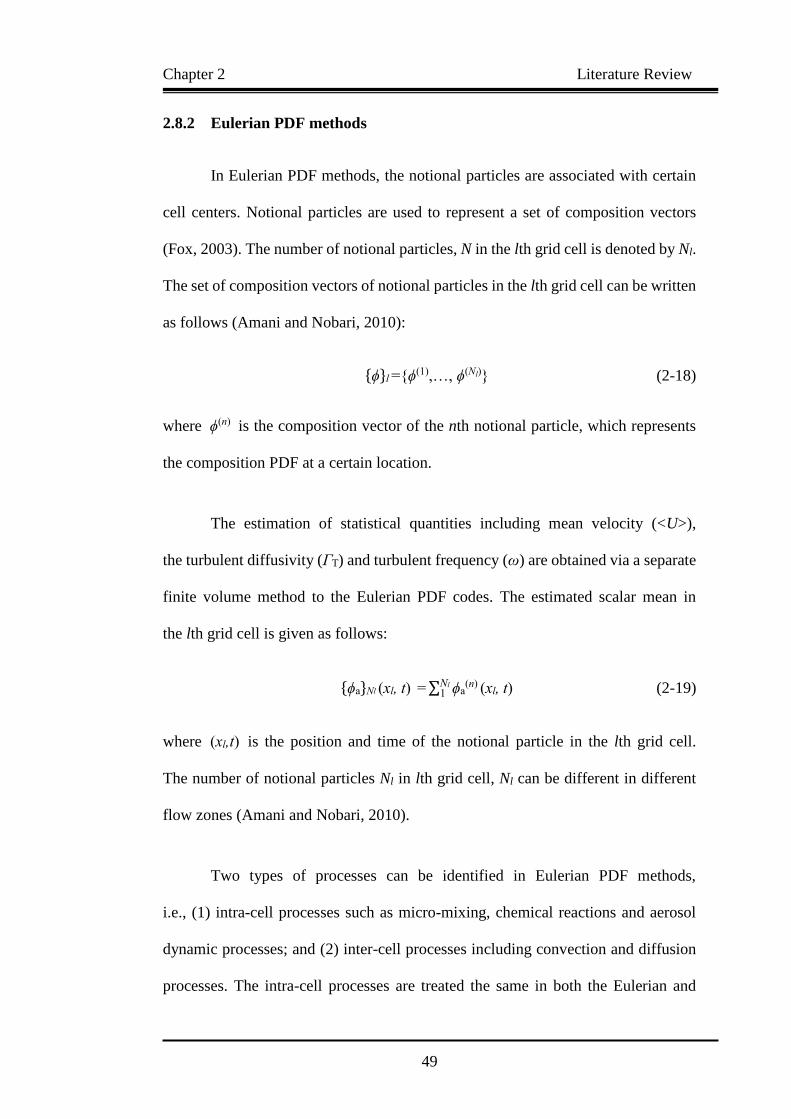
Chapter 2 Literature Review
49
2.8.2 Eulerian PDF methods
In Eulerian PDF methods, the notional particles are associated with certain
cell centers. Notional particles are used to represent a set of composition vectors
(Fox, 2003). The number of notional particles, N in the lth grid cell is denoted by Nl.
The set of composition vectors of notional particles in the lth grid cell can be written
as follows (Amani and Nobari, 2010):
{ϕ}l ={ϕ(1),…, ϕ(Nl)} (2-18)
where ϕ(n) is the composition vector of the nth notional particle, which represents
the composition PDF at a certain location.
The estimation of statistical quantities including mean velocity (<U>),
the turbulent diffusivity (ΓT) and turbulent frequency (ω) are obtained via a separate
finite volume method to the Eulerian PDF codes. The estimated scalar mean in
the lth grid cell is given as follows:
{ϕa}Nl (xl, t) = ∑ ϕa(n)Nl
1 (xl, t) (2-19)
where (xl,t) is the position and time of the notional particle in the lth grid cell.
The number of notional particles Nl in lth grid cell, Nl can be different in different
flow zones (Amani and Nobari, 2010).
Two types of processes can be identified in Eulerian PDF methods,
i.e., (1) intra-cell processes such as micro-mixing, chemical reactions and aerosol
dynamic processes; and (2) inter-cell processes including convection and diffusion
processes. The intra-cell processes are treated the same in both the Eulerian and

Chapter 2 Literature Review
50
Lagrangian PDF methods while the inter-cell processes are treated differently due
to the discrete representation of space in terms of xl (Fox, 2003). The inter-cell flow
variables between a rectangular cell and its four neighboring cells in the Eulerian
PDF method (Pope, 1981) are shown in Figure 2.18.
Figure 2.18 Flow variables for the lth grid cell and four neighboring cells in
Eulerian PDF methods (Fox, 2003).
The basic procedures of numerical implementation of Eulerian PDF methods
are as follows (Fox, 2003):
Step 1: Computing the effective inflow rates for every cell in the flow domain;
Step 2: Computing the numbers of notional particles, that flow into the lth grid cell
from the neighboring cells; and
Step 3: Randomly selecting the new set of notional particles at the lth grid cell with
replacement from the old sets of notional particles. The random selection is carried
out by generating Gaussian random numbers U⊂[0, 1]. It is noteworthy that for
constant-density, statistically stationary flows, the effective flow rates are constant

Chapter 2 Literature Review
51
so that Steps 1 and 2 are completed only once while the Monte Carlo simulation is
advanced by repeating Step 3 and computing intra-cell processes including aerosol
dynamics.
The advantages of Eulerian PDF methods are as follows (Fox, 2003):
The locations of notional particles correspond to the grid cells used in
the finite volume code;
The estimated statistical quantities are found using cell averages since all
notional particles have equal weight;
It is straightforward to implement mixing and chemical reactions and
intra-cell processes;
By combining with finite volume code, it is easy to implement the spatial
transport algorithm on orthogonal grids; and
The computational time expense increases linearly with the total number of
notional particles and the algorithm is easy to parallelize.
Although Eulerian PDF methods have these advantages, they also have fatal
disadvantages (Fox, 2003):
The effective flow rates of every cell are highly grid-dependent and
computing them for arbitrary non-orthogonal grids; Very fine grids are thus
required in order to obtain grid-independent results;
Numerical diffusion remains the principal shortcoming because
the computation of spatial transport is limited to first-order, up-wind schemes,

Chapter 2 Literature Review
52
which leads to a relatively large number of notional particles in order to
reduce statistical error to an acceptable level.
If flow rates vary significantly over the computational domain,
special algorithms are needed to ensure that Nlk ≥ 1.
2.8.3 Lagrangian PDF Methods
In Lagrangian PDF methods, Lagrangian notional particles follow
trajectories in the velocity-composition-physical space originating from random
locations in the physical space. Each notional particle is associated with
corresponding position, composition and velocity. Notional particles with various
weights can be used to represent the inhomogeneity of the flow field.
The information of mean velocity and turbulent fields (i.e., turbulent diffusivity and
frequency) is provided by a finite volume code coupled with the Lagrangian PDF
methods. In the case of constant-density flows, the position and number density of
a notional particle after one time step, Δt can be written as follows (Fox, 2003):
Xn(t+Δt)=Xn(t)+[<U>(Xn(t),t)+∇ΓT (Xn(t),t)]∆t+2ΓT (Xn(t),t)1/2ΔW (2-20)
Nn(t+Δt)=Nn(t)+[CN/2(<Nn(t)>Nn(t))+Wi (N,Y)]∆t (2-21)
Moreover, the composition of a notional particle is given as follows:
dϕ(n) dt⁄ = Cϕ 2⁄ ω (Xn(t),t)(ϕ
α
∗ ϕ
α
n)+S(ϕ(n)) (2-22)
where ΔWi is a Gaussian pseudo-random number for representing the stochastic
fluctuations of Wiener process with mean, <ΔWi>=0 and covariance, <ΔWiΔWj>
= ∆tδi,j , CN is the characteristic scale concerning micro mixing, Wi (N,Y) is the

Chapter 2 Literature Review
53
source term for accounting the variation of particle number density, ΓT is the
turbulent diffusion coefficient, <U> is the average velocity. ϕ(n) is the vector
properties of the notional particles. Cϕ is the characteristic factor and S(ϕ(n)) is the
source term related to chemical reactions and aerosol dynamic processes. The
superscript ‘*’ refers to any notional particle. In Monte Carlo simulation, the
Equations (2-20) to (2-22) are simulated numerically with fractional time stepping.
By applying a local Courant-Freidrich-Lewy (CFL) condition, the time step, Δt can
be determined from the finite volume code (Jenny et al., 2001). For steady flow, the
local time stepping technique can be used in the simulation (Möbus et al., 2001). In
order to maintain uniform statistical error, the particle weights ωn(t) are initialized
according the grid cell volumes and then modified during the Monte Carlo
simulation (Fox, 2003).
The principal steps of the implementation of the Lagrangian PDF methods
are shown in Figure 2.19. The first step is to initialize the particle properties and
turbulence fields. Then the simulation time step Δt is obtained based on the local
CFL condition. The flow field is advanced with the finite volume code and return
turbulent fields. Monte Carlo simulation is then carried out with the turbulent fields
from the finite volume code to compute Xn(Δt). Meanwhile, the intra-cell processes
of micro-mixing, chemical reactions and aerosol dynamic processes are computed
to determine the ϕn(Δt). The particle-field estimates are obtained with the updated
particle properties. The simulation time is then incremented by Δt. The last step is
to check if the simulation time has reached the stopping time.
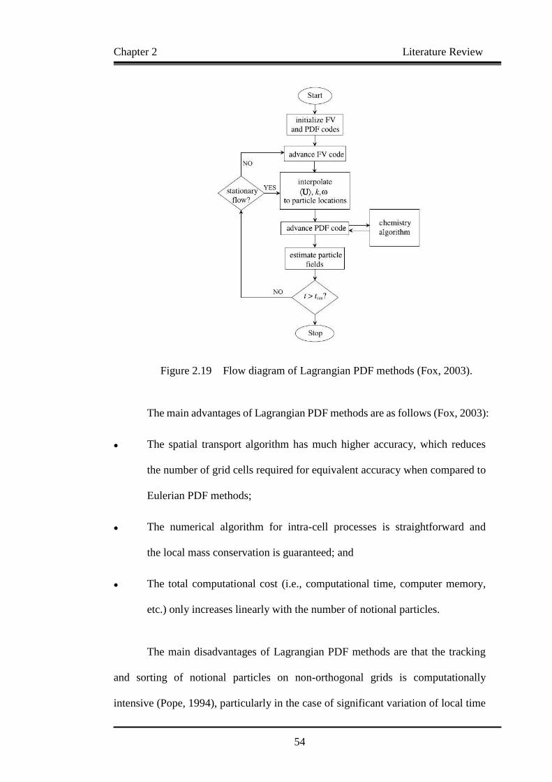
Chapter 2 Literature Review
54
Figure 2.19 Flow diagram of Lagrangian PDF methods (Fox, 2003).
The main advantages of Lagrangian PDF methods are as follows (Fox, 2003):
The spatial transport algorithm has much higher accuracy, which reduces
the number of grid cells required for equivalent accuracy when compared to
Eulerian PDF methods;
The numerical algorithm for intra-cell processes is straightforward and
the local mass conservation is guaranteed; and
The total computational cost (i.e., computational time, computer memory,
etc.) only increases linearly with the number of notional particles.
The main disadvantages of Lagrangian PDF methods are that the tracking
and sorting of notional particles on non-orthogonal grids is computationally
intensive (Pope, 1994), particularly in the case of significant variation of local time
Chapter 2 Literature Review
55
scale over the computational domain. However, local time stepping technique can
be used to reduce the computational cost to some extent (Möbus et al., 2001).
2.8.4 Improvements of the PDF Methods
Besides the Eulerian particle based PDF methods and Lagrangian particle
based PDF methods, stochastic Eulerian field (SEF) PDF methods
(Valiño, 1998; Sabel’nikov and Soulard, 2005; Jaishree and Haworth, 2012;
Consalvi and Nmira, 2016) have been proposed to improve the existing PDF
methods. In the SEF-PDF methods, the notional particles are replaced by notional
Eulerian fields that evolve according to the stochastic partial differential equations
(PDEs) (Celis and Silva, 2015). The stochastic PDEs of the SEF method can be
solved using Eulerian CFD algorithm.
A deterministic Eulerian field method coupled with direct quadrature method
of moments (DQMOM) is developed to a multi-environment PDF-MEPDF method
(Jaishree and Haworth, 2012), which shows higher computational efficiency in
comparison to Eulerian and Lagrangian particle based PDF methods.
More recent improvements of the PDF methods can be found in the literature
(Meyer, 2010; Pope and Tirunagari, 2014; Consalvi and Nmira, 2016).
2.9 Summary of Literature Review
The fundamental concepts, knowledge and methods of aerosol dynamics in
multi-scale systems are reviewed in this chapter to shed light on the development
and state-of-the-art that the researchers have acquired as well as the knowledge gap
for this research area. The literature review is summarized as follows:
Chapter 2 Literature Review
56
1. Aerosol dynamics in multi-scale systems is widely encountered in
engineering and environmental areas including the production of functional
aerosol particles and the prevention of industrial emissions. It is of great
importance to gain a better insight and more intrinsic understanding on
aerosol particles including the generating and evolution mechanisms and
other physiochemical properties.
2. Both experimental and numerical methods play important roles in
the investigation of aerosol dynamics. However, experimental study is quite
limited to relatively simple cases and would be become difficult even
impossible as far as more complex and practical cases are concerned.
Numerical simulation provides an alternative solution to the study of aerosol
dynamics under complex conditions, which is also the focus of the present
study. The advantages of numerical methods are mainly their high capability
and low cost.
3. Numerical methods for aerosol dynamics can be divided into two categories
(i.e., deterministic methods and stochastic methods). Deterministic methods
provide an efficient and accurate approach for the numerical simulation of
aerosol dynamics. However, the inherent limitations of deterministic
methods are also very obvious and difficult to overcome, among which the
inability to provide history information of particles and difficulty to apply to
multi-dimensional and multi-scale problems are fatal in the study of complex
aerosol dynamics. Stochastic methods such as Monte Carlo methods have
unique advantages in dealing with multi-scale and multi-dimensional

Chapter 2 Literature Review
57
problems concerning aerosol dynamics and can provide the history
information and arbitrary number of variables.
4. Various modifications have been made to increase the computational
efficiency and guarantee the computational accuracy of Monte Carlo
methods. In order to solve multi-dimensional problems involving aerosol
dynamic processes, Monte Carlo codes of PBE are coupled to CFD codes to
formulate the coupled CFD-PBM methods, which will also be presented in
Chapters 5 and 6.

Chapter 3 Theoretical Fundamentals of the Present Study
58
Chapter 3 Theoretical Fundamentals of the Present Study
3.1 Introduction
This chapter briefly presents the theoretical fundamentals related to
the newly proposed CFD-Monte Carlo/PDF method including the population
balance equation, Monte Carlo methods, Eulerian-Lagrangian models for
multi-phase flows, and transported PDF methods for turbulent reactive flows.
3.2 Population Balance Equation
3.2.1 Overview
Population balance equations (PBE) in Equation (1-1) can be derived from
the Boltzmann equation (Cercignani, 1988) as shown in Equation
(3-1), which describes a gas particle behavior. PBE is derived to describe how
populations of separate entities evolve or vary in specific properties over time.
They are a set of integro-partial differential equations , which give the behavior of
a population of particles from the analysis of a single particle behavior in local
conditions (Ramkrishna, 2000). Particulate systems feature the birth and death of
particles.
∂f
∂t= (
∂f
∂t)force + (
∂f
∂t)diff + (
∂f
∂t)coll
where f is an unspecified function. The term on the left-hand side (LHS) is
the accumulative term. On the right-hand side (RHS), the first term is the source
(3-1)

Chapter 3 Theoretical Fundamentals of the Present Study
59
term due to external force, the second term is the diffusion term and the last term is
the cumulative effect of inter-particle collisions.
Population balance equation (PBE) is used to describe the evolution of PSD
of particulate systems mathematically (Ramkrishna, 2000), which is a transport
equation of particle number density function or other variables of particles such as
mass and volume dependent on space coordinates, time and particle size.
Depending on actual aerosol dynamic processes, different source terms such as
coagulation, nucleation and growth may appear in PBE, as shown in Equation (2-4).
Combining different source terms into different physical processes, the PBE
(i.e., in Equation (2-4)) is obviously an integro-differential equation. There has been
a large number of research studies concerning the solution of PBE in spatially
homogeneous domain i.e., zero dimensional PBE (Efendiev, 2004; Yu et al., 2009;
Chan et al., 2010; Zhou and Chan, 2011; Geng et al., 2013; Yu and Chan, 2015;
Liu et al., 2015; Liu and Chan, 2017). Zero dimensional PBE here refers to the PBE
expressed in terms of particle number density, which is independent of any spatial
coordinate. The aerosol particles involve no convection or diffusion process.
The particulate phase is not affected by any fluid phase either.
The fundamental assumption in the formulation of PBE is that there is
a uique particle number density for every spatial coordinate in the particle scalar
space (Ramkrishna, 2000), which consists of internal (quantitative characterization
of particle properties) and external (particle location in the physical space)
coordinates. Both the internal and external coordinates of particles may be
discretized under certain conditions. This renders the theoretical basis on which the
discretization of the PBE of particulate systems is performed. Another fundamental

Chapter 3 Theoretical Fundamentals of the Present Study
60
assumption of population balance theory is that the variation rate of any particle state
vector is dependent only on the state of the particles of interest as well as the local
variables of the continuous phase, which renders the coupling between the transport
equation and the population balance equation (Ramkrishna, 2000).
3.2.2 The Self-preserving Behavior of PBE
The self-preserving behavior (also called self-similar behavior) is associated
with the invariant domains in the space of the independent variables within which
the solution to PBE i.e., the reconstructed particle size distribution (PSD) remains
identical or partially identical (Ramkrishna, 2000). A similar transformation for
the PSD function was proposed by Swift and Friedlander (1964) and Friedlander and
Wang (1966) to obtain self-preserving solutions to the PBE, which are asymptotic
forms and independent of the initial PSD.
Based on the assumption that the fraction of the particles in a given size range
is a function only of particle volume normalized by the average particle volume
(Epstein and Ellison, 1987), the similarity transformation can be carried out as
follows:
Firstly, the dimensionless particle size distribution can be written as:
n(v,t)dv
N∞ = ψv(
v
v)d(
v
v)
where v is particle volume, v is the average particle volume, N∞ is the total
number of particles, ψv is a dimensionless function whose form is invariant with
time. By rearranging Equation (3-2), it can be written as:
(3-2)

Chapter 3 Theoretical Fundamentals of the Present Study
61
n(v,t) = (N∞) 2
ϕψv(ηv)
where ηv = v/v = N∞v/ϕ, represents dimensionless particle volume, ϕ is the total
volume of all the particles. Equation (3-3) is the similarity transformation for the
PSD in terms of particle volume, n(v,t) . The boundary conditions are that
n(v,t)→0 for v→0 and v→∞. The form of ψv can be determined in two-steps.
Firstly, the special form of PSD function n(v,t) in Equation (3-3) is tested by
substituting in the Equation (1-1) with appropriate collision frequency function,
β(v,u). If the similar transformation is in accordance with the PBE, one can obtain
an ordinary integro-differential equation for ψv as a dimensionless function of ηv.
Secondly, a solution to the transformed equation is to be found subject to
the following integral constraints:
∫ nvdv = ϕ∞
0
∫ ndv = N∞
∞
0
Based on the assumption that the fraction of the particles in a given size range
is a function only of particle diameter normalized by the average particle diameter,
which is similar to Equation (3-2) and it can be written as:
n(dp,t)d(dp)
N∞ = ψd(
dp
dp
)d(dp
dp
)
Let 𝜂d= dp dp⁄ and dp=(ϕ/N∞)1/3, the obtained similarity transformation for
the PSD in terms of n(dp,t) can be written as:
(3-3)
(3-4)
(3-5)
(3-6)

Chapter 3 Theoretical Fundamentals of the Present Study
62
n(dp,t) = (N∞) 4/3
ϕ1/3 ψd(ηd)
where ηd = dp(N∞/ϕ)1/3 , represents dimensionless particle diameter, dp is
the particle diameter, ψd is a dimensionless function of particle diameter,
and the other variables have the same meaning as in Equation (3-3).
Similarity transformation can be used to obtain closed form solutions for the upper
and lower ends of the PSD while numerical method such as Monte Carlo method
can be used to match the solutions for intermediate-size particles. More details
regarding the existence and feasibility of the self-similar solution to the PBE can be
found in the similarity analysis of PBE (Ramkrishna, 2000).
3.2.3 The Solution of PBE
Except for very special and limited cases to which analytical solutions to
PBE exist (Zhou et al., 2014; Liu and Chan, 2017), it is quite difficult to solve PBE
with analytical methods. Thus, numerical methods e.g., sectional methods
(Jeong and Choi, 2001; Mitrakos et al., 2007;Agarwal and Girshick, 2012), method
of moments (Yu et al., 2008; Lin and Chen, 2013; Park et al., 2013; Chen et al., 2014;
Yu and Chan, 2015; Pollack et al., 2016) as well as Monte Carlo method
(Zhao et al., 2009; Wei, 2013, Zhou et al., 2014; Liu et al., 2015; Liu and Chan,
2017) are often used to solve the PBE. In the present study, Monte Carlo method is
used to obtain the solution of PBE.
Monte Carlo methods are based on artificial realization of the system
behavior (Ramkrishna, 2000). Consider a number of particles distributed in
(3-7)
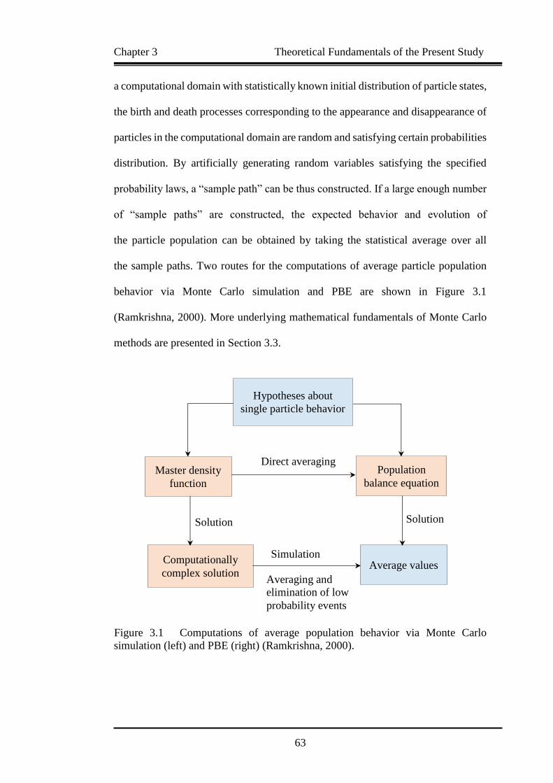
Chapter 3 Theoretical Fundamentals of the Present Study
63
a computational domain with statistically known initial distribution of particle states,
the birth and death processes corresponding to the appearance and disappearance of
particles in the computational domain are random and satisfying certain probabilities
distribution. By artificially generating random variables satisfying the specified
probability laws, a “sample path” can be thus constructed. If a large enough number
of “sample paths” are constructed, the expected behavior and evolution of
the particle population can be obtained by taking the statistical average over all
the sample paths. Two routes for the computations of average particle population
behavior via Monte Carlo simulation and PBE are shown in Figure 3.1
(Ramkrishna, 2000). More underlying mathematical fundamentals of Monte Carlo
methods are presented in Section 3.3.
Figure 3.1 Computations of average population behavior via Monte Carlo
simulation (left) and PBE (right) (Ramkrishna, 2000).
Solution Solution
Simulation
Averaging and
elimination of low
probability events
Direct averaging
Hypotheses about
single particle behavior
Master density
function
Population
balance equation
Computationally
complex solution Average values

Chapter 3 Theoretical Fundamentals of the Present Study
64
3.3 Monte Carlo Methods
3.3.1 Overview
Monte Carlo methods are widely used to solve problems with a probabilistic
interpretation. According to the law of large numbers (Sznitman and Zerner, 1999),
integrals described by the mean value of some random variables can be estimated
by taking the empirical average i.e., the mean values of independent samples out of
the variables. A Markov Chain Monte Carlo (MCMC) sampler (Hastings, 1970) can
be used if the probability distribution of the variables is parameterized. The principal
concept is to design a Markov chain model following certain probability law.
This distribution can be estimated by the empirical knowledge of Monte Carlo
sampler according to the ergodic theorem (Chacon and Ornstein, 1960).
3.3.2 Implementation Procedures
Monte Carlo method is applied to the solution of Boltzmann equation of fluid
flow with finite Knudsen number to formulate the DSMC method (Bird, 1994).
As mentioned in Chapter 2, the basic idea of DSMC is to use a set of numerical
particles to represent the real physical particles. However, only the particle
properties of interest such as momentum and mass are tracked. A random generation
of collision events is justified by the molecular chaos assumption (Maxwell, 1867)
that the velocities of collision particles are independent of position within
a homogenous volume. Baxter and Olafsen (2007) reported the first experimental
observation of molecular chaos, which proves the assumption of molecular chaos is
indeed accurate.
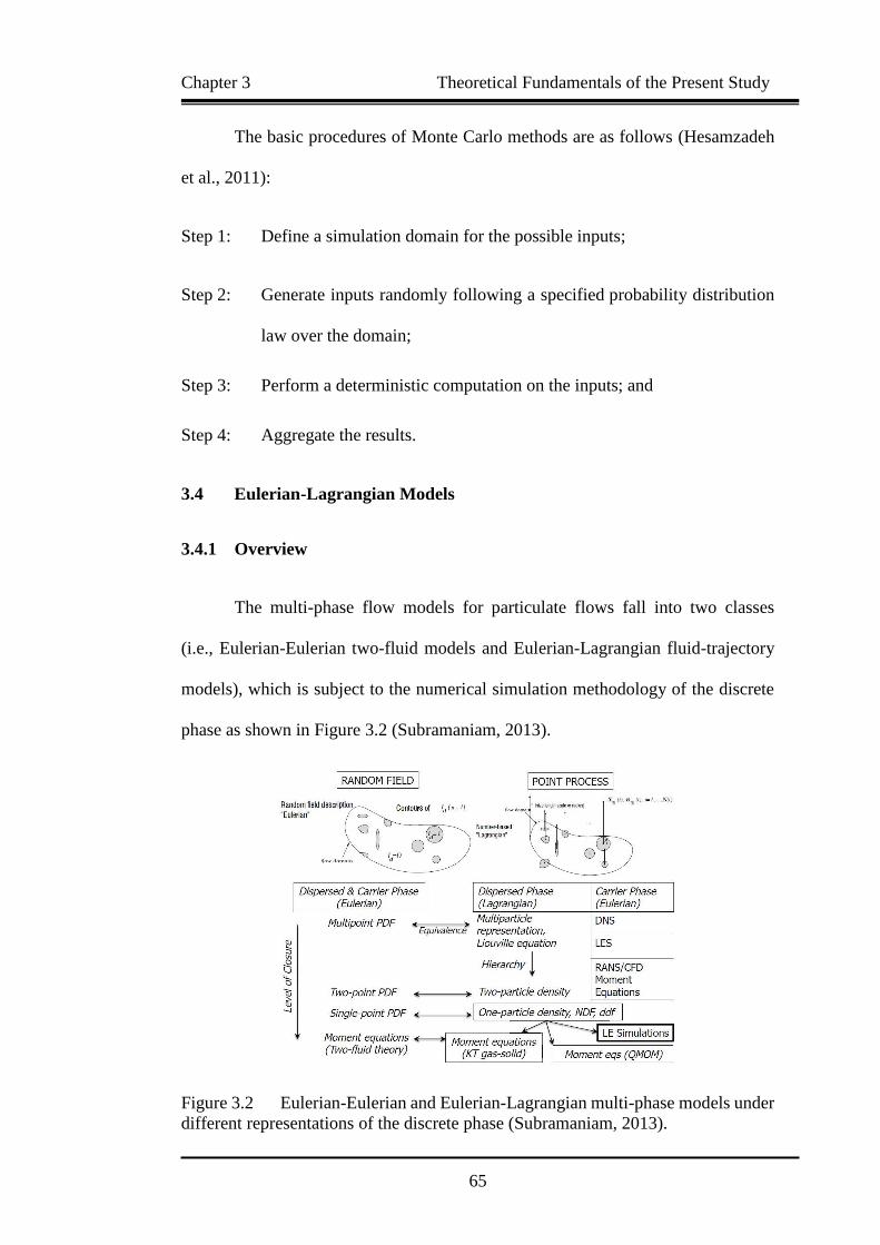
Chapter 3 Theoretical Fundamentals of the Present Study
65
The basic procedures of Monte Carlo methods are as follows (Hesamzadeh
et al., 2011):
Step 1: Define a simulation domain for the possible inputs;
Step 2: Generate inputs randomly following a specified probability distribution
law over the domain;
Step 3: Perform a deterministic computation on the inputs; and
Step 4: Aggregate the results.
3.4 Eulerian-Lagrangian Models
3.4.1 Overview
The multi-phase flow models for particulate flows fall into two classes
(i.e., Eulerian-Eulerian two-fluid models and Eulerian-Lagrangian fluid-trajectory
models), which is subject to the numerical simulation methodology of the discrete
phase as shown in Figure 3.2 (Subramaniam, 2013).
Figure 3.2 Eulerian-Eulerian and Eulerian-Lagrangian multi-phase models under
different representations of the discrete phase (Subramaniam, 2013).

Chapter 3 Theoretical Fundamentals of the Present Study
66
The Eulerian-Eulerian models are formulated if the deterministic PBM
methods e.g. the sectional method is used to simulate the discrete phase
(particulate phase). In the present study, a stochastic PBM-Monte Carlo method is
used for the simulation of aerosol dynamics, which is integrated into the
Eulerian-Lagrangian models for complex aerosol dynamics in turbulent flows. With
the Eulerian-Lagrangian models, the spatiotemporal evolution of particle population
can be obtained, which is rarely reported (Zhao and Zheng, 2013).
3.4.2 Interphase Coupling
In the Eulerian-Lagrangian models, the continuous phase is computed in
an Eulerian reference frame while the discrete phase is computed in a Lagrangian
reference frame (Edge et al., 2011). According to the effect and volume fraction of
the discrete phase, the interaction between discrete phase and continuous phase are
treated with different ways. For fine particles in a dilute flow at low Reynolds
number such as atmospheric aerosols, the effect of particles on the fluid can be
neglected and the solution of the Eulerian-Lagrangian models is simplified to track
particle trajectories in a flow field which is independent of particles (Kruis et al.,
2012; Zucca et al., 2007). Fine particles are airborne particles which are smaller than
coarse particles. They have an aerodynamic diameter of 2.5 µm or less (PM2.5).
However, the momentum exchange between particles and fluid must be
considered if particles have high enough momentum to affect the motion of fluid.
Moreover, if the volume fraction of particles in a grid cell is high, the continuity and
momentum equations of fluid need to be modified to model the effective viscosity
of the particle suspension in the viscous stress term (Patankar and Joseph, 2001).
Chapter 3 Theoretical Fundamentals of the Present Study
67
The mutual coupling between the fluid phase and particulate phase for the
inter-particle interactions can be taken into account with the mutiphase particle-in-
cell (MP-PIC) method (Andrews and O’Rourke, 1996; Snider, 2001). In the MP-
PIC method, where the particle phase is treated both as continuous and discrete
phases, an accurate mapping from Lagrangian particles is used to associate a particle
with a computational grid. While on the grid, the continuum derivative terms that
treat the particle phase as a fluid are readily evaluated and then mapped back to
individual particles (Andrews and O’Rourke, 1996). For two-way coupling,
the particle source in cell (PSI-Cell) method (Crowe et al., 1977) can be used,
which regards the particle phase as a source of mass, momentum, and energy to the
gaseous phase (Novozhilov et al., 1997).
3.5 Transported PDF Methods for Turbulent Reactive Flows
3.5.1 Overview
Probability density function (PDF) methods have become one of the most
promising and powerful approaches for accommodating the effects of turbulent
fluctuations in velocity and chemical composition in CFD-based modeling of
turbulent reactive flows (Haworth, 2010). Transported PDF methods have also been
developed to overcome the closure problems due to interaction between turbulence
and particle evolution in turbulent reactive flows by many researchers (Pope, 1981;
Pope, 1985; Valino, 1998; Sabel’nikov and Soulard, 2005; Meyer, 2010; Pope and
Tirunagari, 2014; Consalvi and Nmira, 2016).
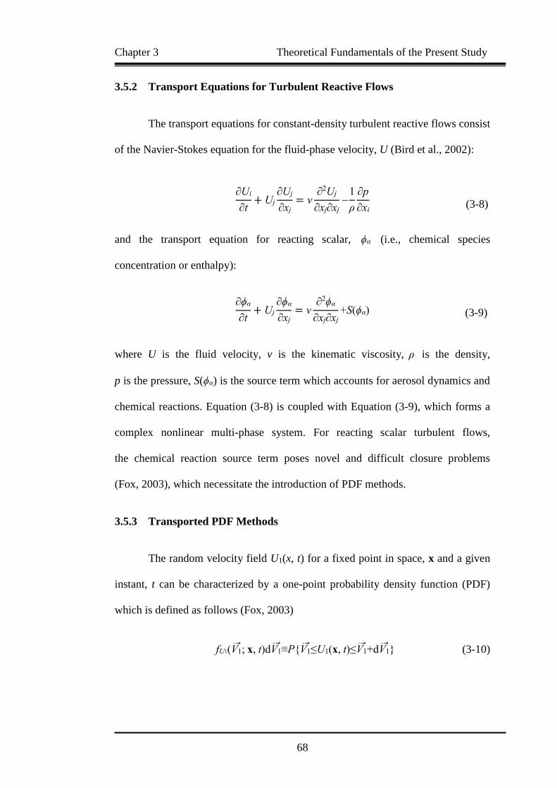
Chapter 3 Theoretical Fundamentals of the Present Study
68
3.5.2 Transport Equations for Turbulent Reactive Flows
The transport equations for constant-density turbulent reactive flows consist
of the Navier-Stokes equation for the fluid-phase velocity, U (Bird et al., 2002):
∂Ui
∂t+ Uj
∂Uj
∂xj= v
∂2Uj
∂xj∂xj
1
ρ
∂p
∂xi
and the transport equation for reacting scalar, ϕα (i.e., chemical species
concentration or enthalpy):
∂ϕα
∂t+ Uj
∂ϕα
∂xj= v
∂2ϕα
∂xj∂xj+S(ϕα)
where U is the fluid velocity, v is the kinematic viscosity, ρ is the density,
p is the pressure, S(ϕα) is the source term which accounts for aerosol dynamics and
chemical reactions. Equation (3-8) is coupled with Equation (3-9), which forms a
complex nonlinear multi-phase system. For reacting scalar turbulent flows,
the chemical reaction source term poses novel and difficult closure problems
(Fox, 2003), which necessitate the introduction of PDF methods.
3.5.3 Transported PDF Methods
The random velocity field U1(x, t) for a fixed point in space, x and a given
instant, t can be characterized by a one-point probability density function (PDF)
which is defined as follows (Fox, 2003)
fU1(V 1; x, t)dV 1≡P{V 1≤U1(x, t)≤V 1+dV 1} (3-10)
(3-9)
(3-8)
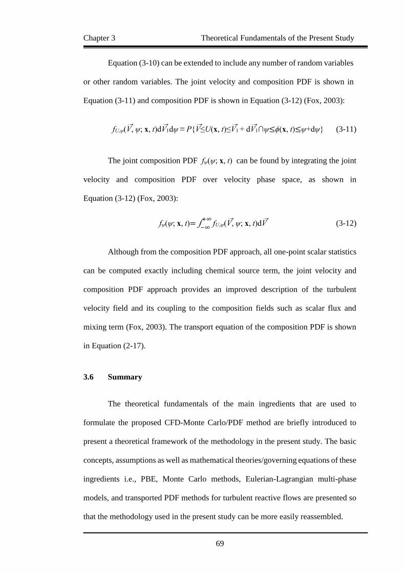
Chapter 3 Theoretical Fundamentals of the Present Study
69
Equation (3-10) can be extended to include any number of random variables
or other random variables. The joint velocity and composition PDF is shown in
Equation (3-11) and composition PDF is shown in Equation (3-12) (Fox, 2003):
fU,ψ(V , ψ; x, t)dV 1dψ ≡ P{V ≤U(x, t)≤V 1 + dV 1∩ψ≤ϕ(x, t)≤ψ+dψ} (3-11)
The joint composition PDF fψ(ψ; x, t) can be found by integrating the joint
velocity and composition PDF over velocity phase space, as shown in
Equation (3-12) (Fox, 2003):
fψ(ψ; x, t)=∫ fU,ψ(V , ψ; x, t)dV +∞
−∞ (3-12)
Although from the composition PDF approach, all one-point scalar statistics
can be computed exactly including chemical source term, the joint velocity and
composition PDF approach provides an improved description of the turbulent
velocity field and its coupling to the composition fields such as scalar flux and
mixing term (Fox, 2003). The transport equation of the composition PDF is shown
in Equation (2-17).
3.6 Summary
The theoretical fundamentals of the main ingredients that are used to
formulate the proposed CFD-Monte Carlo/PDF method are briefly introduced to
present a theoretical framework of the methodology in the present study. The basic
concepts, assumptions as well as mathematical theories/governing equations of these
ingredients i.e., PBE, Monte Carlo methods, Eulerian-Lagrangian multi-phase
models, and transported PDF methods for turbulent reactive flows are presented so
that the methodology used in the present study can be more easily reassembled.

Chapter 4 Zero-dimensional Monte Carlo Simulation of Aerosol Dynamics
70
Chapter 4 Zero-dimensional Monte Carlo Simulation of
Aerosol Dynamics
4.1 Introduction
The purpose of this chapter is to study the complex aerosol dynamic
processes by using this newly proposed and developed stochastically weighted
operator splitting Monte Carlo (SWOSMC) method. Stochastic weighted particle
method and operator splitting method are coupled to formulate the SWOSMC
method for the numerical simulation of particle-fluid systems undergoing
the complex simultaneous aerosol dynamic processes.
This SWOSMC method is first validated by comparing the numerical
simulation results of constant rate coagulation and linear rate condensation with the
corresponding analytical solutions. Coagulation and nucleation cases are further
studied whose results are compared with the sectional method in excellent agreement.
This SWOSMC method has also demonstrated its high numerical simulation
capability when used to deal with simultaneous aerosol dynamic processes including
coagulation, nucleation and condensation. The comparison between the numerical
method used here (SWOSMC method) and the analytical solution is shown in
Table 4.1.
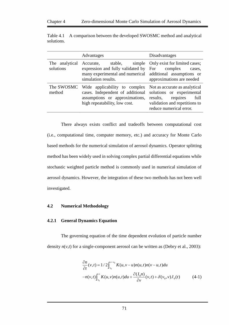
Chapter 4 Zero-dimensional Monte Carlo Simulation of Aerosol Dynamics
71
Table 4.1 A comparison between the developed SWOSMC method and analytical
solutions.
Advantages Disadvantages
The analytical
solutions
Accurate, stable, simple
expression and fully validated by
many experimental and numerical
simulation results.
Only exist for limited cases;
For complex cases,
additional assumptions or
approximations are needed
The SWOSMC
method
Wide applicability to complex
cases. Independent of additional
assumptions or approximations,
high repeatability, low cost.
Not as accurate as analytical
solutions or experimental
results, requires full
validation and repetitions to
reduce numerical error.
There always exists conflict and tradeoffs between computational cost
(i.e., computational time, computer memory, etc.) and accuracy for Monte Carlo
based methods for the numerical simulation of aerosol dynamics. Operator splitting
method has been widely used in solving complex partial differential equations while
stochastic weighted particle method is commonly used in numerical simulation of
aerosol dynamics. However, the integration of these two methods has not been well
investigated.
4.2 Numerical Methodology
4.2.1 General Dynamics Equation
The governing equation of the time dependent evolution of particle number
density n(v,t) for a single-component aerosol can be written as (Debry et al., 2003):
0
0
0
00 0
( , ) 1 / 2 ( , ) ( , ) ( , )
( )( , ) ( , ) ( , ) ( , ) ( , ) ( )
v v
v
v
nv t K u v u n u t n v u t du
t
I nn v t K u v n u t du v t v v J t
v
(4-1)
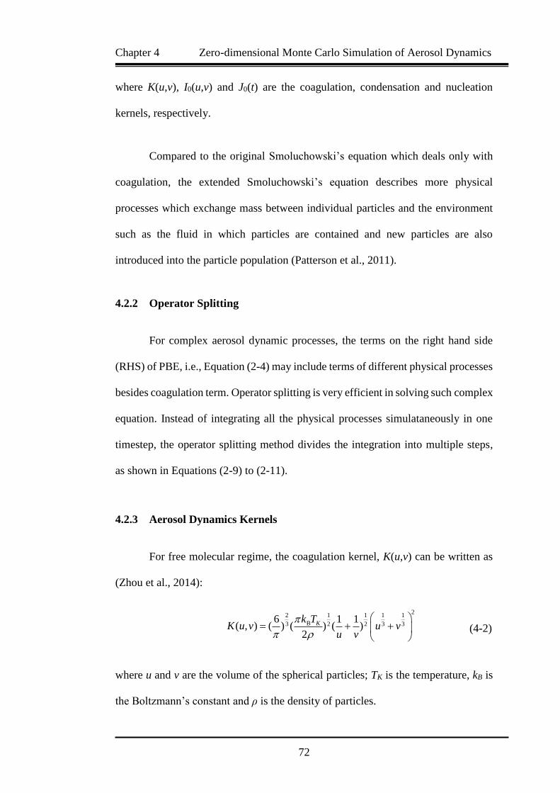
Chapter 4 Zero-dimensional Monte Carlo Simulation of Aerosol Dynamics
72
where K(u,v), I0(u,v) and J0(t) are the coagulation, condensation and nucleation
kernels, respectively.
Compared to the original Smoluchowski’s equation which deals only with
coagulation, the extended Smoluchowski’s equation describes more physical
processes which exchange mass between individual particles and the environment
such as the fluid in which particles are contained and new particles are also
introduced into the particle population (Patterson et al., 2011).
4.2.2 Operator Splitting
For complex aerosol dynamic processes, the terms on the right hand side
(RHS) of PBE, i.e., Equation (2-4) may include terms of different physical processes
besides coagulation term. Operator splitting is very efficient in solving such complex
equation. Instead of integrating all the physical processes simulataneously in one
timestep, the operator splitting method divides the integration into multiple steps,
as shown in Equations (2-9) to (2-11).
4.2.3 Aerosol Dynamics Kernels
For free molecular regime, the coagulation kernel, K(u,v) can be written as
(Zhou et al., 2014):
22 1 11 1
B3 3 32 26 1 1
( , ) ( ) ( ) ( )2
Kk TK u v u v
u v
where u and v are the volume of the spherical particles; TK is the temperature, kB is
the Boltzmann’s constant and ρ is the density of particles.
(4-2)

Chapter 4 Zero-dimensional Monte Carlo Simulation of Aerosol Dynamics
73
In continuous regime, for the size of spherical particles, u and v,
the coagulation kernel can be written as (Debry et al., 2003):
1/3 1/3
B K air( , ) 2 / 3 [2 ( / ) ( / ) ]K u v k T v u u v
where μair is the viscosity of air and the other parameters have the same physical
meanings as that in Equation (4-2).
The homogeneous nucleation rate can be generally written as
(Seinfeld and Pandis, 1998):
J0(t)=Cexp(∆G*/kBT)
where ∆G* is the free energy that is required to form a stable nucleus and C is
a constant which is related to vapor pressure.
As condensation/evaporation process involves the relaxation to an
equilibrium state between aerosol and gas phases for one chemical species
(Debry et al., 2003), the kernels are thus proportional to the pressure difference
between the bulk gas and the equilibrium pressure:
I0(v,t) = CI exp(pi∞ p
i
eq)
where CI is a constant which is related to the diffusion species and temperature,
pi∞ and pi
eq are the vapor pressure and the equilibrium vapor pressure of species,
i from the particle, respectively.
(4-3)
(4-4)
(4-5)
Chapter 4 Zero-dimensional Monte Carlo Simulation of Aerosol Dynamics
74
4.2.4 Non-dimensionalization
The GDE Equation (4-1) is non-dimensionalized based on the relative mass
density, q(v,t) of aerosol particles (Debry et al., 2003) which can be expressed as
Equation (4-6):
q(v,t)=q(v,t)
Q0, Q0 = ∫ q0(v)dv
∞
0
where q(v,t) is the mass density of aerosol particles and Q0 is the total initial mass
of aerosol particles.
Substituting n(v,t) into Equation (4-1) with q(v,t), it can be expressed as
(Debry et al., 2003):
0
0
0
0
0
0
0 0 00
0
( , )( , ) 1 / 2 ( , ) ( , )
, ,( , )( , ) ( , )
( ) ( )( , ) ( , )
v v
v
v
q K u v uv t Q q u t q v u t du
t v u
I v t q v tK u vq v t Q q u t du
u v
I q v J tv t v v
v Q
4.2.5 Algorithm Formulation
The main idea of the present method is to introduce stochastic weights to
various numerical particles according to the mass change caused by different aerosol
dynamic processes in order to increase the numerical stability of Monte Carlo
method. Operator splitting technique is used to treat stochastic process
(i.e., coagulation) and deterministic processes (i.e., condensation, nucleation etc.)
separately with corresponding methods to reduce computational time for
the simulation of complex aerosol dynamics. The idea of using numerical particles
(4-6)
(4-7)
Chapter 4 Zero-dimensional Monte Carlo Simulation of Aerosol Dynamics
75
with varying mass weights (Debry et al., 2003) is adopted herein, where the i-th
numerical particle is associated with a varying mass weight, wi(t) of real aerosol
particle of size, yi(t), thus the i-th numerical particle now stands for a number of
wi(t)/yi(t) of real aerosol particles.
The introduction of such a varying mass weight to numerical particles in
stochastic simulation of simultaneous aerosol dynamic processes is necessary and
well justified. When mass weights are adhered to numerical particles (i.e., numerical
particles are connected with a certain mass of real aerosols), the total number of
numerical particles remains constant and no re-sampling is needed for coagulation
process (Eibeck and Wagner, 2001). This is because the total mass of real aerosol
particles remains constant in coagulation process although the total number of real
aerosol particles decreases.
If the numerical particles are directly connected with the number of real
aerosol particles and no further up sampling (adding new particles to
the particle-fluid system) is conducted, the decreasing number of numerical particles
may cause severe numerical diffusion as coagulation converges on an infinite
number of numerical particles. However, for some other aerosol dynamic processes
including nucleation, condensation, evaporation, deposition and removal, the total
mass of aerosol particles in the particle-fluid system actually varies with time.
By introducing varying mass weights to numerical particles, the weights, wi(t) will
evolve with time for mass-varying process such as condensation and evaporation.
In here, nucleation is conducted by creating a certain mass of new particles according
to nucleation rate which is independent of pre-existing particles. The integration

Chapter 4 Zero-dimensional Monte Carlo Simulation of Aerosol Dynamics
76
details for an individual process will be presented in Section 4.3.2. The main
algorithm of stochastically weighted operator splitting Monte Carlo (SWOSMC)
method over a time period [0, T] is presented as follows:
Initialization: setting of the following quantities:
0 0[ , ,i iwy01,2, .. ].., i N
;
Operator splitting over time loop [0, T]:
Integration of Equation (4-7) from tk to tk+1 = tk + τk, where τk is the time step
determined previously:
(i) Integration of coagulation based on Monte Carlo based methods
(Gillespie, 1972);
(ii) Integration of condensation using an ODE solver from Zhou et al., (2014);
(iii) Integration of nucleation: creation of new particles, J; and
(iv) Updating the particle-fluid system and when t >T, stop the simulation and
take average over the results.
4.3 Numerical Setup
4.3.1 Time Step Determination
According to Debry et al., (2003), the time scales for different physical
processes can be calculated as Equations (4-8) to (4-10) in order to allow an accurate
integration result as well as avoid too much computational time:

Chapter 4 Zero-dimensional Monte Carlo Simulation of Aerosol Dynamics
77
For coagulation of aerosols, yik, y
jk:
coag
0
=( , )
k
j
k kkj i j
yt
KQ y yw
For condensation/evaporation of aerosols, yjk,
cond/evap
0
=( , )
k
j
k
ki
yt
y tI
For nucleation of aerosols:
∆tnucl =Q0
v0J0(t)
To ensure an accurate integration, the time step should be less than the
minimum of all the time scales (Zhao et al., 2005) from Equations (4-8) to (4-10)
which is set as the minimum time step.
4.3.2 Integration Details
The system state after a time step is calculated by integrating over a time step.
Noting that a varying mass weight is used, only condensation/evaporation processes
that cause the mass change to the particle-fluid system will have numerical particles
with varying weights.
For integration of coagulation, the collision criterion should be met.
The volume of particle i after a splitting time step becomes the total volume of
particle i and its collision partner, while the weight of i-th numerical particle remains
(4-8)
(4-9)
(4-10)

Chapter 4 Zero-dimensional Monte Carlo Simulation of Aerosol Dynamics
78
unchanged. For the i-th numerical particle at k-th time step, the integration procedure
is written as:
1/2 0( , )
, if k kk
k k k Ji i Jiki i Ji k
Ji
KQ y ywry y y
y
=min( )( , )
k
Jik k k k
Ji i Ji
yc
KQw y y
where yik+1/2, y
ik, y
Jik are the volume size after the collision step, the volume of i-th
particle and the volume collided with i-th particle at k-th time step, respectively.
For the criterion part, r is a random number uniformly distributed over [0, 1],
τk is the defined time step based on the minimum coagulation time scale and is also
defined as the collison probability is within [0, 1], c is a constant which is usually
0( , )
k kkJi i Ji
kk
Ji
KQ y yw
y equal to 0.1 (Debry et al., 2003).
For integration of condensation, it is performed via integration using
a self-adaptive fifth-order Runge-Kutta method (Zhou et al., 2014) over the splitting
time step of varying weight function, which is determined by the mechanistic rate of
condensation. For the i-th numerical particle at k-th time step, the results obtained
from the above coagulation step are used as input for this step, the integration
procedure is written as:
dyi
dt=I0(yi,t),
dwi
dt=wi
I0(yi,t)
yi
yik+1=y
ik+1/2+∆tI0(y
ik+1/2, tk), wi
k+1=wik+1/2
yik+1
yik+1/2
where yik+1/2, y
ik+1 are the volume size, wi
k+1/2, wik+1 are the weights, I0(yi
k+1/2, tk)
and I0(yi,t) are the condensation rates after the condensation step and that obtained
(4-11b)
(4-12b)
(4-11a)
(4-12a)
Chapter 4 Zero-dimensional Monte Carlo Simulation of Aerosol Dynamics
79
from the previous coagulation step for the i-th particle and the k-th time step,
respectively. Δt is the integration time step.
For integration of nucleation, only a certain mass of new particles with
the minimum nucleus volume, v0 are created and added to the particle-fluid system.
For the i-th newly created particle, it is defined as:
10 0 0, 1, ( )k
i c kiv m v J t ty w
where yik+1 is the volume size of the i-th newly created particle, wi is the weight of
the i-th newly created particle, J0(tk) is the nucleation rate mass of of the i-th newly
created particle, mc is the total mass of all the newly created particles within one time
step and v0 is the initial volume size of the newly created particles.
4.3.3 Initial Conditions and Cases with Analytical Solutions
4.3.3.1 Initial Conditions
The initial particle number density is 1.01018 /m3 and initial particle dimeter
is set as 1.24 nm for Case 1 (constant rate coagulation and linear rate condensation
case) and Case 2 (constant rate coagulation and nucleation) so that the following
simple dimensionless expressions for moments can be obtained. The initial
conditions of the other cases in the present study can be found in Frenklach and
Harris (1987). All the studied cases in the present study are listed in Table 4.2.
These cases are selected to represent the typical aerosol dynamic processes taking
place in the actual particle-fluid systems such as particulate emission from vehicles
and industrial boilers, aerosol formation, collodial solution, etc. These studied cases
are so arranged that the complexity of numerical simulation cases increases from
(4-13)
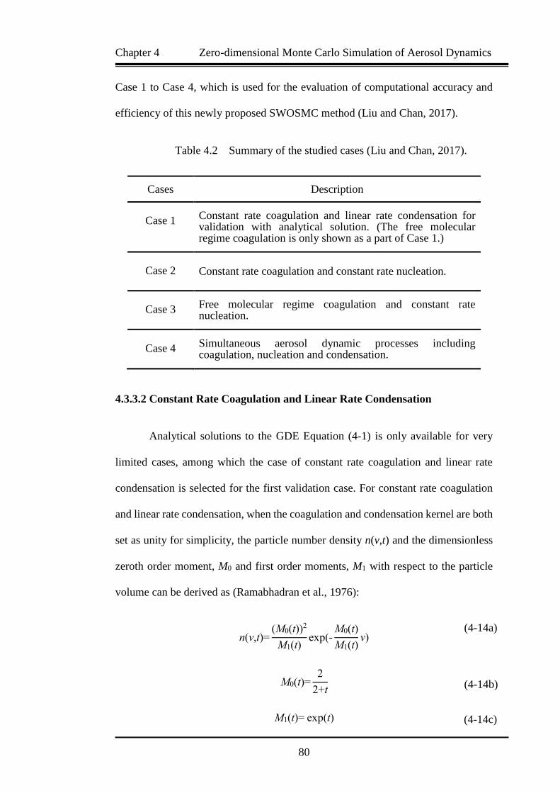
Chapter 4 Zero-dimensional Monte Carlo Simulation of Aerosol Dynamics
80
Case 1 to Case 4, which is used for the evaluation of computational accuracy and
efficiency of this newly proposed SWOSMC method (Liu and Chan, 2017).
Table 4.2 Summary of the studied cases (Liu and Chan, 2017).
Cases Description
Case 1 Constant rate coagulation and linear rate condensation for validation with analytical solution. (The free molecular regime coagulation is only shown as a part of Case 1.)
Case 2 Constant rate coagulation and constant rate nucleation.
Case 3 Free molecular regime coagulation and constant rate nucleation.
Case 4 Simultaneous aerosol dynamic processes including coagulation, nucleation and condensation.
4.3.3.2 Constant Rate Coagulation and Linear Rate Condensation
Analytical solutions to the GDE Equation (4-1) is only available for very
limited cases, among which the case of constant rate coagulation and linear rate
condensation is selected for the first validation case. For constant rate coagulation
and linear rate condensation, when the coagulation and condensation kernel are both
set as unity for simplicity, the particle number density n(v,t) and the dimensionless
zeroth order moment, M0 and first order moments, M1 with respect to the particle
volume can be derived as (Ramabhadran et al., 1976):
n(v,t)=(M0(t))
2
M1(t)exp(-
M0(t)
M1(t)v)
M0(t)=2
2+t
M1(t)= exp(t) (4-14c)
(4-14a)
(4-14b)

Chapter 4 Zero-dimensional Monte Carlo Simulation of Aerosol Dynamics
81
4.3.3.3 Constant Rate Coagulation and Nucleation
If both coagulation and nucleation rates are constant (i.e., both are set as unity
for simplicity in the present study), an analytical solution is available to Equation
(4-1). The analytical solutions of relative particle number density and relative
particle volume concentration can be expressed as (Maisels et al., 2004):
N
N0=B
1+Btanh(τ0/2)
B+tanh(τ0/2)
V
V0=1+
B
2τ0
where V and V0 are the total volume of particles at time, t and at initial time,
t0, respectively. N and N0 are the number density of particles at time, t and at initial
time, t0 respectively. B, E (in Equation (4-17)) and τ0 are dimensionless parameters
determined by the initial conditions and the detailed expressions can be found in
Maisels et al. (2004).
4.3.3.4 Simultaneous Coagulation, Nucleation and Condensation
For simultaneous aerosol dynamic processes, if the nucleation, coagulation,
condensation rates and monomer concentration are constant, the analytical solution
to these simultaneous processes including coagulation, nucleation and condensation
exists (Maisels et al., 2004). The analytical expression of relative particle number
denstity is given in Equation (4-15) since condensation involves no change in
the particle number. The analytical expression of the relative particle volume
concentration for simultaneous coagulation, nucleation and condensation is written
as:
(4-15)
(4-16)

Chapter 4 Zero-dimensional Monte Carlo Simulation of Aerosol Dynamics
82
V
V0=1+[(
B
2+E)τ0+2Eln(
1+exp(-τ0)
2+
1-exp(-τ0)
2B)]
where all the parameters in Equation (4-17) have the same physical meanings with
those in Equations (4-15) and (4-16). More information of this case study can be
found in Liu et al. (2015).
4.3.4 Calculation of Maximum Relative Error
The maximum relative error used to evaluate the numerical simulation
results is defined as:
max = {√[(X(t) X0(t)) X0(t)⁄ ]2}max
where max is the maximum relative error, X(t) is the numerical simulation results
obtained with this newly proposed SWOSMC method, and X0(t) is the reference
value for comparison.
4.4 Results and discussion
4.4.1 Initial Validation
This newly proposed SWOSMC method (Liu and Chan, 2017) is first
validated for constant rate coagulation and linear rate condensation processes.
The dimensionless zeroth order moment, M0 which is proportional to the number
density of particles, is shown in Figure 4.1. An increasing number of numerical
particles are used for the numerical simulation. It can be seen that the numerical
simulation results agree well with the analytical solution when only 1000 numerical
(4-17)
(4-18)

Chapter 4 Zero-dimensional Monte Carlo Simulation of Aerosol Dynamics
83
particles are used, which shows the good capability of the SWOSMC method in
dealing with simultaneous coagulation and condensation processes.
Figure 4.1 Zeroth order moment, M0 under coagulation and condensation
processes for SWOSMC (Liu and Chan, 2017) versus the analytical solution
(Ramabhadran et al., 1976) where N is the number of numerical particles used in
each simulation run.
An excellent agreement between the dimensionless first order moment, M1
obained by the SWOSMC method and analytical solution is also observed in
Figure 4.2. The exponentially increasing M1 with respect to simulation time
represents the rapid increase of the total volume of particles in the numerical
simulation particle-fluid system due to condensation.
2
4
6
8
10
4321
Time (-3s)
SWOSMC method
Sectional method
P
arti
cle
nu
mb
er d
ensi
ty (
17 /
m3)
00.4
0.5
0.6
0.7
0.8
0.9
1.0
2.01.51.00.5
M0
Time (s)
N=50 SWOSMC
N=500 SWOSMC
N=1000 SWOSMC
N=2000 SWOSMC
Analytical solution
0

Chapter 4 Zero-dimensional Monte Carlo Simulation of Aerosol Dynamics
84
Figure 4.2 First order moment, M1 under coagulation and condensation processes
for SWOSMC (Liu and Chan, 2017) versus the analytical solution (Ramabhadran et
al., 1976) where the number of numerical particles, N used in each simulation run is
1000.
Figure 4.3 shows another application of the SWOSMC method to free
molecular regime coagulation and the numerical simulation results is validated by
comparing to the sectional method (Prakash et al., 2003). Excellent agreement can
be also observed between the particle number density obtained by these two methods
with the maximum relative error (by taking the sectional method as reference) of
less than 1% during the whole simulation time.
2
4
6
8
10
4321
Time (-3s)
SWOSMC method
Sectional method
P
arti
cle
nu
mb
er d
ensi
ty (
17 /
m3)
01
2
3
4
5
6
7
2.01.51.00.5
M1
SWOSMC method
Analytical solution
Time (s)
0

Chapter 4 Zero-dimensional Monte Carlo Simulation of Aerosol Dynamics
85
Figure 4.3 Particle number density under free molecular regime coagulation for
SWOSMC (Liu and Chan, 2017) versus the sectional method (Prakash et al., 2003)
where the number of numerical particles, N used in each simulation run is 1000.
4.4.2 Constant Rate Coagulation and Nucleation
For constant rate coagulation and nucleation, an increasing number of
numerical particles are used in the SWOSMC method. Figure 4.4 shows the relative
particle number density, N/N0 obtained via the SWOSMC method and the analytical
solution (Maisels et al., 2004), respectively. It can be seen that the SWOSMC
method agrees well with the analytical solution with increased number of numerical
particles. The increasing relative particle number density implies the nucleation is
dominant within the simulation time. As the simulation proceeds, some statistical
fluctuations can be observed, but the maximum relative error compared with the
analytical solution remains less than 2% during the whole simulation time, which
also proves the reliability of this newly proposed SWOSMC method (Liu and Chan,
2017).
2
4
6
8
10
4321
Time (-3s)
SWOSMC method
Sectional method
P
arti
cle
nu
mb
er d
ensi
ty (
17 /
m3)
0
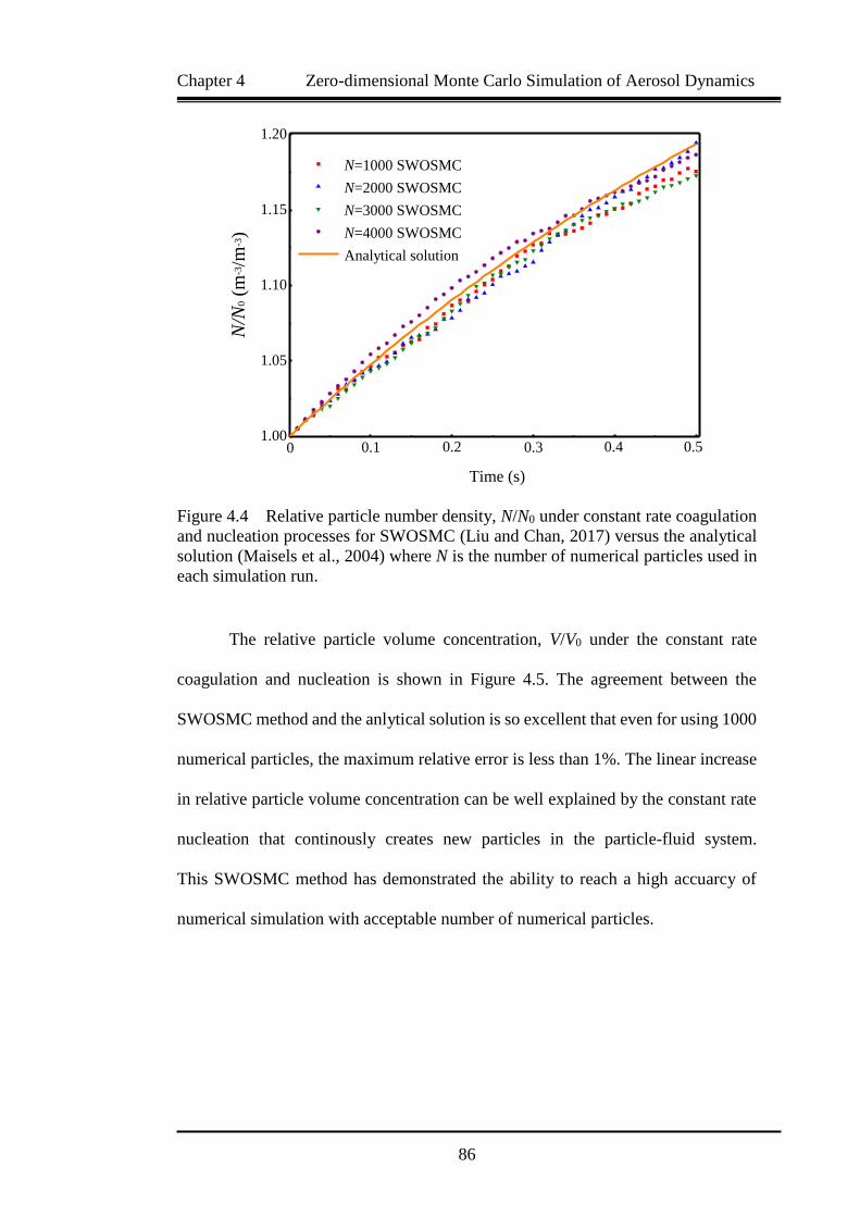
Chapter 4 Zero-dimensional Monte Carlo Simulation of Aerosol Dynamics
86
Figure 4.4 Relative particle number density, N/N0 under constant rate coagulation
and nucleation processes for SWOSMC (Liu and Chan, 2017) versus the analytical
solution (Maisels et al., 2004) where N is the number of numerical particles used in
each simulation run.
The relative particle volume concentration, V/V0 under the constant rate
coagulation and nucleation is shown in Figure 4.5. The agreement between the
SWOSMC method and the anlytical solution is so excellent that even for using 1000
numerical particles, the maximum relative error is less than 1%. The linear increase
in relative particle volume concentration can be well explained by the constant rate
nucleation that continously creates new particles in the particle-fluid system.
This SWOSMC method has demonstrated the ability to reach a high accuarcy of
numerical simulation with acceptable number of numerical particles.
1.00
1.05
1.10
1.15
1.20
0.50.40.30.20.10
N/N
0 (
m-3/m
-3)
N=1000 SWOSMC
N=2000 SWOSMC
N=3000 SWOSMC
N=4000 SWOSMC
Analytical solution
Time (s)

Chapter 4 Zero-dimensional Monte Carlo Simulation of Aerosol Dynamics
87
Figure 4.5 Relative particle volume concentration, V/V0 under constant rate
coagulation and nucleation processes for SWOSMC (Liu and Chan, 2017) versus
the analytical solution (Maisels et al., 2004) where N is the number of numerical
particles used in each simulation run.
4.4.3 Free Molecular Regime Coagulation and Constant Rate Nucleation
Figure 4.6 shows the evolution history of particle number density of
simultaneous free molecular regime coagulation and constant rate nucleation
obtained via the SWOSMC method (Liu and Chan, 2017) and the sectional method
(Prakash et al., 2003). A very satisfactory agreement can be found between the two
methods for even 100 numerical particles used for the SWOSMC method,
which demonstrates the good applicability and computational efficency of this
SWOSMC method in solving simultaneous free molecular regime coagulation and
constant nucleation problem. As the number of numerical particles increases from
100 to 2000, the maximum relative error between these two methods remains
basically the same, which implies that 100 numerical particles is already enough to
reach very good agreement compared with the sectional method. Some fluctuations
can be found for numerical simulation with different number of numerical particles
1.0
1.1
1.2
1.3
1.4
1.5
0.50.40.30.20.10
N=1000 SWOSMC
N=2000 SWOSMC
N=3000 SWOSMC
N=4000 SWOSMC
Analytical solution
V/V
0 (
m3/m
3)
Time (s)
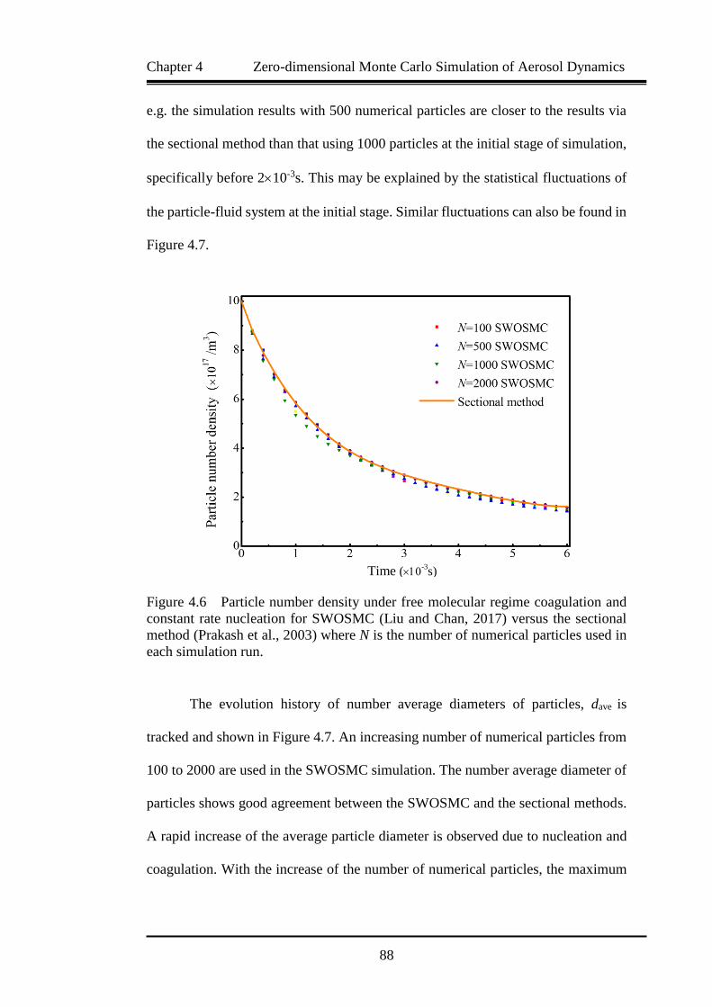
Chapter 4 Zero-dimensional Monte Carlo Simulation of Aerosol Dynamics
88
e.g. the simulation results with 500 numerical particles are closer to the results via
the sectional method than that using 1000 particles at the initial stage of simulation,
specifically before 210-3s. This may be explained by the statistical fluctuations of
the particle-fluid system at the initial stage. Similar fluctuations can also be found in
Figure 4.7.
Figure 4.6 Particle number density under free molecular regime coagulation and
constant rate nucleation for SWOSMC (Liu and Chan, 2017) versus the sectional
method (Prakash et al., 2003) where N is the number of numerical particles used in
each simulation run.
The evolution history of number average diameters of particles, dave is
tracked and shown in Figure 4.7. An increasing number of numerical particles from
100 to 2000 are used in the SWOSMC simulation. The number average diameter of
particles shows good agreement between the SWOSMC and the sectional methods.
A rapid increase of the average particle diameter is observed due to nucleation and
coagulation. With the increase of the number of numerical particles, the maximum
2
4
6
8
10
4321
Time (-3s)
SWOSMC method
Sectional method
P
arti
cle
nu
mb
er d
ensi
ty (
17 /
m3)
0
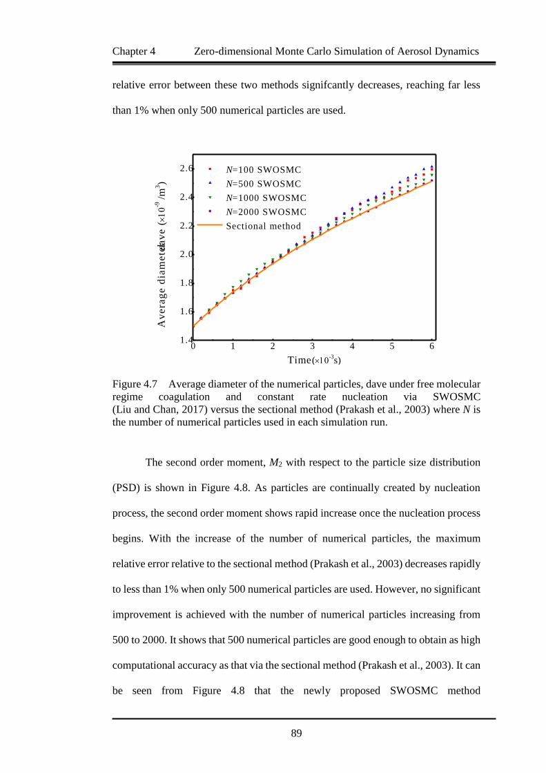
Chapter 4 Zero-dimensional Monte Carlo Simulation of Aerosol Dynamics
89
relative error between these two methods signifcantly decreases, reaching far less
than 1% when only 500 numerical particles are used.
Figure 4.7 Average diameter of the numerical particles, dave under free molecular
regime coagulation and constant rate nucleation via SWOSMC
(Liu and Chan, 2017) versus the sectional method (Prakash et al., 2003) where N is
the number of numerical particles used in each simulation run.
The second order moment, M2 with respect to the particle size distribution
(PSD) is shown in Figure 4.8. As particles are continually created by nucleation
process, the second order moment shows rapid increase once the nucleation process
begins. With the increase of the number of numerical particles, the maximum
relative error relative to the sectional method (Prakash et al., 2003) decreases rapidly
to less than 1% when only 500 numerical particles are used. However, no significant
improvement is achieved with the number of numerical particles increasing from
500 to 2000. It shows that 500 numerical particles are good enough to obtain as high
computational accuracy as that via the sectional method (Prakash et al., 2003). It can
be seen from Figure 4.8 that the newly proposed SWOSMC method
2
4
6
8
10
4321
Time (-3s)
SWOSMC method
Sectional method
P
art
icle
nu
mb
er
de
nsi
ty (
17 /
m3)
00 1 2 3 4 5 61.4
1.6
1.8
2.0
2.2
2.4
2.6
N=100 SWOSMC
N=500 SWOSMC
N=1000 SWOSMC
N=2000 SWOSMC
Sectional method
Time (-3s)
Av
era
ge
dia
me
ter da
ve
(
-9 /
m3)
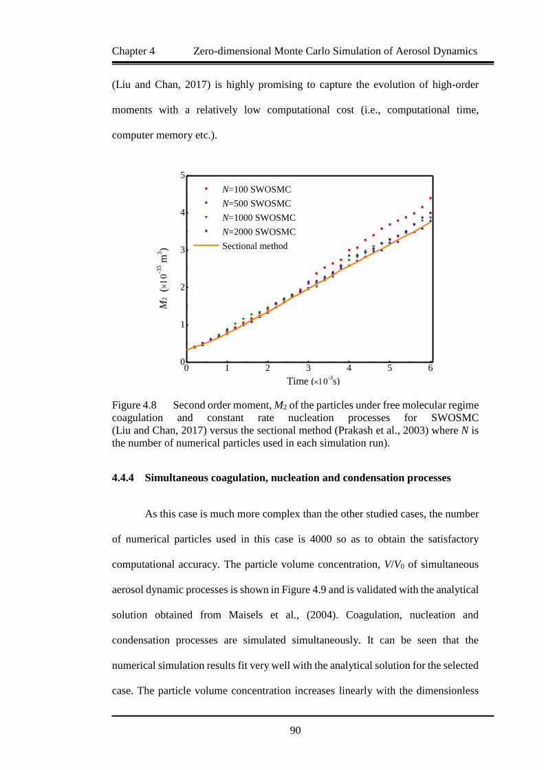
Chapter 4 Zero-dimensional Monte Carlo Simulation of Aerosol Dynamics
90
(Liu and Chan, 2017) is highly promising to capture the evolution of high-order
moments with a relatively low computational cost (i.e., computational time,
computer memory etc.).
Figure 4.8 Second order moment, M2 of the particles under free molecular regime
coagulation and constant rate nucleation processes for SWOSMC
(Liu and Chan, 2017) versus the sectional method (Prakash et al., 2003) where N is
the number of numerical particles used in each simulation run).
4.4.4 Simultaneous coagulation, nucleation and condensation processes
As this case is much more complex than the other studied cases, the number
of numerical particles used in this case is 4000 so as to obtain the satisfactory
computational accuracy. The particle volume concentration, V/V0 of simultaneous
aerosol dynamic processes is shown in Figure 4.9 and is validated with the analytical
solution obtained from Maisels et al., (2004). Coagulation, nucleation and
condensation processes are simulated simultaneously. It can be seen that the
numerical simulation results fit very well with the analytical solution for the selected
case. The particle volume concentration increases linearly with the dimensionless
2
4
6
8
10
4321
Time (-3s)
SWOSMC method
Sectional method
Par
ticl
e n
um
ber
den
sity
(
17 /
m3)
00 1 2 3 4 5 60
1
2
3
4
5
N=100 SWOSMC
N=500 SWOSMC
N=1000 SWOSMC
N=2000 SWOSMC
Sectional method
Time (-3s)
M2 (
-35 m
3)
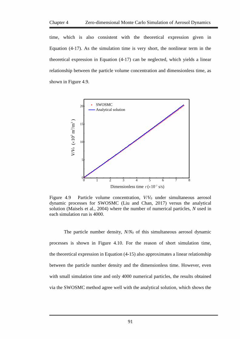
Chapter 4 Zero-dimensional Monte Carlo Simulation of Aerosol Dynamics
91
time, which is also consistent with the theoretical expression given in
Equation (4-17). As the simulation time is very short, the nonlinear term in the
theoretical expression in Equation (4-17) can be neglected, which yields a linear
relationship between the particle volume concentration and dimensionless time, as
shown in Figure 4.9.
Figure 4.9 Particle volume concentration, V/V0 under simultaneous aerosol
dynamic processes for SWOSMC (Liu and Chan, 2017) versus the analytical
solution (Maisels et al., 2004) where the number of numerical particles, N used in
each simulation run is 4000.
The particle number density, N/N0 of this simultaneous aerosol dynamic
processes is shown in Figure 4.10. For the reason of short simulation time,
the theoretical expression in Equation (4-15) also approximates a linear relationship
between the particle number density and the dimensionless time. However, even
with small simulation time and only 4000 numerical particles, the results obtained
via the SWOSMC method agree well with the analytical solution, which shows the
0 1 2 3 4 5 6 7 80
5
10
15
20
Dimensionless time (10 s/s)
V
/V0 (
10
2 m
3/m
3 )
SWOSMC
Analytical solution

Chapter 4 Zero-dimensional Monte Carlo Simulation of Aerosol Dynamics
92
high potential of this newly proposed SWOSMC method in solving simultaneous
full processes in complex aerosol dynamics.
Figure 4.10 Particle number concentration, N/N0 under simultaneous aerosol
dynamic processes for SWOSMC (Liu and Chan, 2017) versus the analytical
solution (Maisels et al., 2004) where the number of numerical particles, N used in
each simulation run is 4000.
4.4.5 Parametric analysis of the studied cases
The main simulation parameters are presented in Table 4.3 for evaluation
purpose of this newly proposed and developed SWOSMC method
(Liu and Chan, 2017). It can be seen that with the increase of the complexity from
Case 1 to Case 4, an increasing computational time is needed for a fixed number of
numerical particles. However, for a certain case, the computational error is inversely
proportional to the square root of the total number of the numerical particles (Oran
et al., 1998). It also suggests that further optimization of this new SWOSMC method
is needed in order to improve the computational efficiency and accuracy for the
complex particle-fluid systems. Compared with the sectional method
0 1 2 3 4 5 6 7 80
5
10
15
20
Dimensionless time (10 s/s)
N/N
0 (
10
2 m
3/m
3 )
SWOSMC
Analytical solution
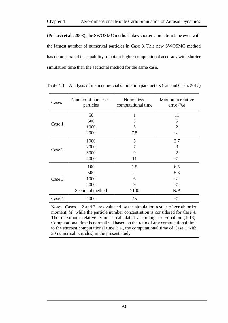
Chapter 4 Zero-dimensional Monte Carlo Simulation of Aerosol Dynamics
93
(Prakash et al., 2003), the SWOSMC method takes shorter simulation time even with
the largest number of numerical particles in Case 3. This new SWOSMC method
has demonstrated its capability to obtain higher computaional accuracy with shorter
simulation time than the sectional method for the same case.
Table 4.3 Analysis of main numercial simulation parameters (Liu and Chan, 2017).
Cases Number of numerical
particles
Normalized
computational time
Maximum relative
error (%)
Case 1
50 1 11
500 3 5
1000 5 2
2000 7.5 <1
Case 2
1000 5 3.7
2000 7 3
3000 9 2
4000 11 <1
Case 3
100 1.5 6.5
500 4 5.3
1000 6 <1
2000 9 <1
Sectional method >100 N/A
Case 4 4000 45 <1
Note: Cases 1, 2 and 3 are evaluated by the simulation results of zeroth order
moment, M0 while the particle number concentration is considered for Case 4.
The maximum relative error is calculated according to Equation (4-18).
Computational time is normalized based on the ratio of any computational time
to the shortest computational time (i.e., the computational time of Case 1 with
50 numerical particles) in the present study.
Chapter 4 Zero-dimensional Monte Carlo Simulation of Aerosol Dynamics
94
4.5 Summary
The simulation results of this newly proposed and developed stochastically
weighted operator splitting Monte Carlo (SWOSMC) method (Liu and Chan, 2017)
are fully validated with corresponding analytical solution (Maisels et al., 2004) and
the sectional method (Prakash et al., 2003) for various aerosol dynamic processes
(i.e., coagulation, condensation and nucleation) in different flow regimes.
This validated SWOSMC method also offers higher capacity of numerical
simulation for solving simultaneous aerosol dynamic processes occurring in
complex particle-fluid systems. Further development of this new method will be
presented in the study of multi-dimensional and inhomogeneous aerosol dynamic
processes of turbulent particle-fluid systems in Chapter 5.
Chapter 5 CFD-PBM Simulation of Aerosol Dynamics in Turbulent Flows
95
Chapter 5 CFD-PBM Simulation of Aerosol Dynamics in
Turbulent Flows
5.1 Introduction
A computational fluid dynamics (CFD) coupling with a Monte Carlo
(CFD-Monte Carlo) method is presented to simulate complex aerosol dynamics in
turbulent flows. A Lagrangian particle method based probability density function
(PDF) transport equation is formulated to solve the population balance equation
(PBE) of aerosol particles. The formulated CFD-Monte Carlo method allows
investigating the interaction between turbulence and aerosol dynamics and
incorporating individual aerosol dynamic kernels as well as obtaining full particle
size distribution (PSD). Several typical cases of aerosol dynamic processes including
turbulent coagulation, nucleation and growth are studied and compared to the
sectional method with excellent agreement. Coagulation in both laminar and
turbulent flows is simulated and compared to demonstrate the effect of turbulence
on aerosol dynamics. The effect of jet Reynolds (Rej) number on aerosol dynamics
in turbulent flows is fully investigated for each of the studied cases.
The results demonstrate that Rej has significant impact on a single aerosol dynamic
process (e.g. coagulation) and the competitive and simultaneous aerosol dynamic
processes in turbulent flows. This newly proposed and validated CFD-Monte
Carlo/PDF method renders an efficient method for simulating complex aerosol
dynamics in turbulent flows and provides a better insight into the interaction between
turbulence and the full PSD of aerosol particles. The novelty of the present study is
to investigate the effect of Rej number on the PSD of typical aerosol dynamic
processes in turbulent flows. The enhancing effect of turbulence on aerosol dynamic

Chapter 5 CFD-PBM Simulation of Aerosol Dynamics in Turbulent Flows
96
processes as well as the competition and transition between different aerosol
dynamic processes are proved and analyzed. A new particle tracking method with
high computational efficiency is adopted in the Monte Carlo simulation.
Moreover, the operator splitting technique recently proposed by Liu and Chan (2017)
for solving simultaneous aerosol dynamic processes is also used to increase
the computational efficiency and accuracy.
5.2 Numerical Methodology
5.2.1 Governing Equations of Aerosol Dynamics in Turbulent Flows
The governing equations of the coupled fluid dynamics-aerosol dynamics in
turbulent flows include the PBE in terms of particle number density (i.e., Equation
(1-1)) as well as continuity, momentum equations (i.e., Navier-Stokes equations)
and energy equation, which are written as:
∇⋅u (x, t)= 0 (5-1)
∂u (x, t)/∂t + (u (x, t)⋅∇)u (x, t)= νk∇2u (x, t) ∇P (x, t)⋅∇ ρ⁄ (5-2a)
∂T (x, t)/∂t + (u (x, t)⋅∇2T = ke∇2T (x, t) + H ρ⁄ cp (5-2b)
where u is the velocity of the carrier fluid phase, νk is the kinematic viscosity,
which is assumed constant, x is the coordinates of particles, P is the pressure, ρ is
the fluid density, ke is the heat conductivity, H is the source of energy and cp is
the specific heat capacity, T is temperature. An in-house time dependent Reynolds-
Averaged Navier Stokes (RANS) code and k-ε turbulence model (also used in the
transported PDF method of Akridis and Rigopoulos (2015)) are used together with
the following transported PDF method.
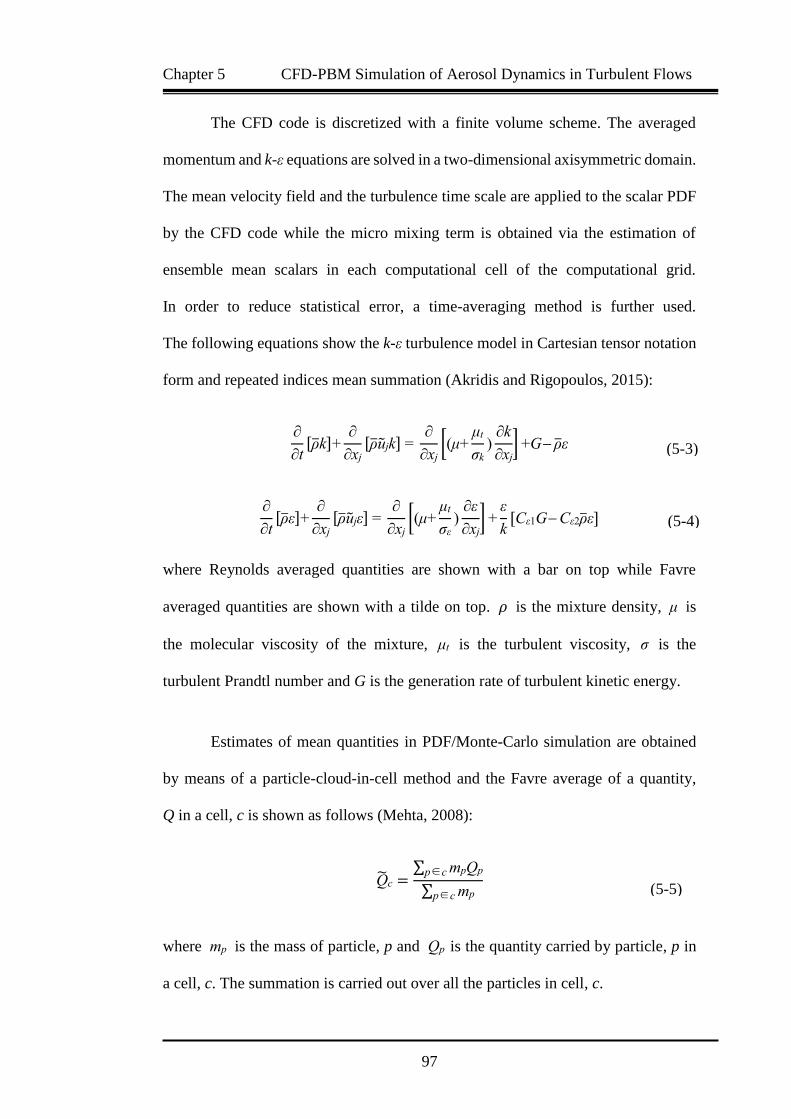
Chapter 5 CFD-PBM Simulation of Aerosol Dynamics in Turbulent Flows
97
The CFD code is discretized with a finite volume scheme. The averaged
momentum and k-ε equations are solved in a two-dimensional axisymmetric domain.
The mean velocity field and the turbulence time scale are applied to the scalar PDF
by the CFD code while the micro mixing term is obtained via the estimation of
ensemble mean scalars in each computational cell of the computational grid.
In order to reduce statistical error, a time-averaging method is further used.
The following equations show the k-ε turbulence model in Cartesian tensor notation
form and repeated indices mean summation (Akridis and Rigopoulos, 2015):
∂
∂t[ρk]+
∂
∂xj
[ρujk] = ∂
∂xj[(μ+
μt
σk)
∂k
∂xj] +G ρε
∂
∂t[ρε]+
∂
∂xj
[ρujε] = ∂
∂xj[(μ+
μt
σε)
∂ε
∂xj] +
ε
k[Cε1G Cε2ρε]
where Reynolds averaged quantities are shown with a bar on top while Favre
averaged quantities are shown with a tilde on top. 𝜌 is the mixture density, μ is
the molecular viscosity of the mixture, μt is the turbulent viscosity, σ is the
turbulent Prandtl number and G is the generation rate of turbulent kinetic energy.
Estimates of mean quantities in PDF/Monte-Carlo simulation are obtained
by means of a particle-cloud-in-cell method and the Favre average of a quantity,
Q in a cell, c is shown as follows (Mehta, 2008):
Qc =∑ mpQpp∈c
∑ mpp∈c
where mp is the mass of particle, p and Qp is the quantity carried by particle, p in
a cell, c. The summation is carried out over all the particles in cell, c.
(5-3)
(5-4)
(5-5)

Chapter 5 CFD-PBM Simulation of Aerosol Dynamics in Turbulent Flows
98
The PBE in terms of particle number density, n(v, x, t), a function of particle
volume as well as of space coordinates and time, can be written as Equation (5-6),
in which n(v, x, t) is written as n(v) for simplicity:
∂n(v)/∂t + ∇(u⋅n(v))+ ∂(G(Y1, Y2,…,Ym,v) ∂v⁄ ⋅n(v))
=Dp∇2n(v) + Bn(Y1, Y2,…,Ym,v)⋅δ(v v0)
+ 1/2 ∫ K(u, vu)n(u, t)n(vu, t)dun(v,t) ∫ K(u, v)n(u, t)du∞
0
v-v0
v0
(5-6)
The terms in PBE i.e., Equation (5-6) from the left-hand side to the right-hand side
are:
Accumulation term of the particle number density.
Convection term in physical space.
Condensation/growth term in phase space, where G(Y1, Y2,…,Ym, v) is the
growth kernel, a function species concentration Ym and particle volume v.
Particle diffusion term, where Dp is the diffusion coefficients of particles.
Nucleation term, where Bn (Y1, Y2,…,Ym, v) is the nucleation kernel, Ym is
a function of species concentration and v is particle volume. This term
contributes a source for particle with the size of v0 which is the minimum
particle size of the nuclei.
Coagulation term, which consists of two parts. The first part is the birth part
accounting for all the possible gains in particle number density of particles
with size of v due to the coagulation between particle of size (v-v0) and v0.
The factor 1/2 is used to prevent double counting the coagulation events.

Chapter 5 CFD-PBM Simulation of Aerosol Dynamics in Turbulent Flows
99
The second part is the death part accounting for all the loss of particles with
size of v due to all the possible combinations. K(u,v) is the coagulation kernel
dependent on the size of colliding pairs.
5.2.2 PDF Transport Equation Formulation
The derivation of PDF formulation for aerosol dynamics in turbulent flows
is based on the work of Rigopoulos (2007). First, a joint multipoint PDF of the mass
concentration and particle number density of species at full size range is introduced
so that the expected PSD at any point can be determined:
Y(x, t), n(v, x, t) ≡ f (Y, N; x, t) (5-7)
where Y ≡ y1, y2, …, ym and N ≡ n1, n2, …, nn have the following constraints:
ya < Ya(x, t) < ya+dy (5-8a)
n < N(vi, x, t) < n+dn (5-8b)
and the normalization property is also satisfied:
∫ ∫ f (Y, N; x, t)dY dN = 1∞
0
1
0 (5-9)
5.2.2.1 Discretization of the Continuous PBE
As the continuous function of n(v, x, t) is needed for the source terms
(e.g., the nucleation growth/condensation and coagulation), the continuous PBE is
discretized based on the approximation of infinite space points with finite space
points (Rigopoulos and Jones, 2003):
N(v) ≈ {N(v1), N(v2), …, N(vn)} = {N1, N2,…, Nn} (5-10)

Chapter 5 CFD-PBM Simulation of Aerosol Dynamics in Turbulent Flows
100
The growth term in Equation (5-6) is discretized as follows:
∂(G(Y1, Y2,…,Ym,v) ∂v⁄ ⋅n(v))
≈ (G(Y1, Y2,…,Ym,v)⋅(Ni
vi-vi-1-
Ni-1
vi-vi-1) + Ni ⋅∂(G(Y1, Y2,…,Ym,v) ∂v⁄ )
= G1(Y1, Y2,…,Ym,v)⋅Ni + G2(Y1, Y2,…,Ym,v)⋅Ni-1 (5-11)
where
G1 = G(Y1, Y2,…,Ym,v)⋅ 1 (vivi-1⁄ ) + ∂(G(Y1, Y2,…,Ym,vi) ∂v⁄
G2 = G(Y1, Y2,…,Ym,v)⋅ 1 (vivi-1⁄ )
The nucleation term in Equation (5-3) is discretized as:
B(Y1, Y2,…,Ym,v)⋅δ(vv0)
≈ B(Y1, Y2,…,Ym,v)/[1/2(v1 v0)]+B(Y1, Y2,…,Ym,v)/[1/2(v0 0)]
= B1(Y1, Y2,…,Ym) (5-12)
The coagulation term is discretized as:
C ≈ 1/2 ∑ ai-j,j(vi-j,vj)⋅Ni-jNjNi ∑ a'i-j,j(vi,vj)∙Nji-1j=1
i-1j=1 (5-13)
where C represents the coagulation term in Equation (5-6), ai-j,j and a'i-j,j are the
coagulation kernels.
Based on the above discretized terms, the discretized form of PBE can be written as:
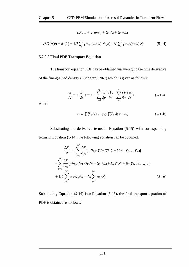
Chapter 5 CFD-PBM Simulation of Aerosol Dynamics in Turbulent Flows
101
∂Ni/∂t + ∇(u⋅Ni) + G1⋅Ni + G2⋅Ni-1
= Dp∇2n(v) + B1(Y) + 1/2 ∑ ai-j,j(vi-j,vj)⋅Ni-jNj Ni ∑ a'i-j,j(vi,vj)⋅Nji-1j=1
i-1j=1 (5-14)
5.2.2.2 Final PDF Transport Equation
The transport equation PDF can be obtained via averaging the time derivative
of the fine-grained density (Lundgren, 1967) which is given as follows:
∂f
∂t = <
∂F
∂t> = < ∑
∂F
∂ya
∂Ya
∂t
M
a=1
∑∂F
∂ni
∂Ni
∂t
N
i =1
> (5-15a)
where
𝐹 = ∏ δ(Ya ya)∙Ma=1 ∏ δ(Ni ni)
Ni=1 (5-15b)
Substituting the derivative terms in Equation (5-15) with corresponding
terms in Equation (5-14), the following equation can be obtained:
∂F
∂t = ∑
∂F
∂ya[ ∇(u⋅Ya)+D∇2Ya+w(Y1, Y2,…,Ym)]
M
a=1
∑∂F
∂ni[∇(u⋅Ni)-G1⋅Ni G2⋅Ni-1 + Dp∇2Ni + B1(Y1, Y2,…,Ym)
N
i =1
+ 1/2 ∑ ai,j⋅Ni-jNj Ni ∑ ai,j⋅Nj
i1
j=1
i1
j=1
] (5-16)
Substituting Equation (5-16) into Equation (5-15), the final transport equation of
PDF is obtained as follows:

Chapter 5 CFD-PBM Simulation of Aerosol Dynamics in Turbulent Flows
102
∂f
∂t = u∙f <u'∇F>∑∑ D
∂2(∇Ya∙∇Ya∙F)
∂ya∂yb
m
b=1
m
a=1
∑∑ Dp
∂2(∇Ni∙∇Ni∙F)
∂ni∂nj
m
b=1
m
a=1
∂
∂ya[B1(y1, y2,…,ym)∙f ]
+∂
∂ni[(G1(y1, y2,…,ym)niG2∙ni-1)∙f ]
−∑∂
∂ni[1/2 ∑ (ai,j∙ni-jnj )
i-1
j=1
∙f ] + ∑∂
∂ni[ni ∑[(ai,j∙Nj)∙f ]
𝑛
𝑖=1
𝑛
𝑖=1
n
i=1
(5-17)
5.2.3 Monte Carlo Simulation of the PDF Transport Equation
The Monte Carlo method developed by Fox (2003) is further extended to
solve the PDF transport equation of aerosol dynamics in turbulent flows.
The underlying concept of this Monte Carlo method is to simulate a number of
stochastic entities, whose evolution statistics obtained via stochastic differential
equations as well as CFD method approximate the PDF of interest.
The stochastic model for the evolution of particle position and particle number
density used to advance PDF is as follows:
Xn(t+∆t) = Xn(t)+[<U>(Xn(t),t)+∇ΓT (Xn(t),t)]∆t+2ΓT (X
n(t),t)1/2ΔW (5-18)
Nn(t+Δt) = Nn(t)+[CN/2(<Nn(t)> Nn(t))+Wi (N,Y)]∆t (5-19)
where ΔWi is a Gaussian pseudo-random number for representing the stochastic
fluctuations of Wiener process with mean <ΔWi> = 0 and covariance <ΔWi ∙ ΔWj>
= ∆tδi,j , CN is the characteristic scale concerning micro mixing, Wi (N,Y) is the
source term for accounting the variation of particle number density, ΓT is the
turbulent diffusion coefficient, <U> is the average velocity.
Chapter 5 CFD-PBM Simulation of Aerosol Dynamics in Turbulent Flows
103
It is noteworthy that in the simulation of coagulation event of particles with
a certain size, instead of looping several neighboring grid cells which contain a large
amount of notional particles, the loop checking will be carried out within only one
grid cell. It implies that the loop checking will be performed over all the particles
located within the grid cell to counter check if they are involved in coagulation
events. The possible grid cell in which the tracked particles may be located after
a time step, Δt is determined before sorting its possible coagulation partners.
Then Monte Carlo method is applied to determine the probability of certain aerosol
dynamic events in the certain grid cell. It is reasonably assumed that all the
coagulation events within one time step, Δt of a tracked notional particle take place
in one same grid cell. By this assumption, the computational time spent on sorting
particles for coagulation is greatly reduced, thus increasing the computational
efficiency.
The procedures of one loop of Monte Carlo simulation are as follows (several
repetitions may be carried out in order to reduce the statistical errors caused by
the intrinsic nature Monte Carlo method):
Step 1: Initialization of particle properties (particle size distribution,
particle number density and initial positions) and the turbulence field (average
velocity < U >(x, 0) , turbulence frequency 𝜔(x, 0) and turbulent diffusion
coefficient ΓT (x, 0);
Step 2: Based on the turbulence field parameters in the previous step,
calculate the time step to advance the transport PDF according to Equation (5-20)
i.e., constraints of Courant-Friedrichs-Lewy (CFL) number and minimum

Chapter 5 CFD-PBM Simulation of Aerosol Dynamics in Turbulent Flows
104
characteristic time scale of all the aerosol dynamic processes. The final time step is
calculated as follows:
∆t = c⋅Minimum{ NCFL ( ∑ui
ΔLi
mi=1 )⁄ , tcoag, tnuclea, tgrowth} (5-20)
where c is a constant factor to guarantee the decoupling between the particle
dynamics processes and the particle transport, NCFL is the maximum CFL number
which is also a constant (NCFL = 0.5 is used in the present study). m is the number of
dimensions (for two-dimensional flow, m = 2), ui is the velocity at i-direction,
Li is the width of the grid cell in i-direction, tcoag, tnuclea, tgrowth are the characteristic
time scale of coagulation, nucleation and growth processes, respectively which are
dependent on the local field parameters (i.e., mass concentration, particle size etc.);
Step 3: Advance the computing of flow field with a finite volume method (FVM)
CFD code and return the turbulence field parameters including average velocity,
<U>(x, ∆t) , turbulence frequency, ω(x, ∆t) and turbulent diffusion coefficient,
ΓT (x, ∆t);
Step 4: Monte Carlo method is used to calculate the particle position Xn(∆t) and
particle number density, Nn(Δt). A sorting algorithm based on random number is
used to determine the Npl particles and renumber them according to their grid cells.
The intra cell process, particularly aerosol dynamic processes, are advanced to
determine the source terms in the PDF transport equation (in Equation (5-17)).
Step 5: Update the particle properties accordingly. Using these updated particle
properties, particle-field estimates are constructed by particle source in cell (PSIC)
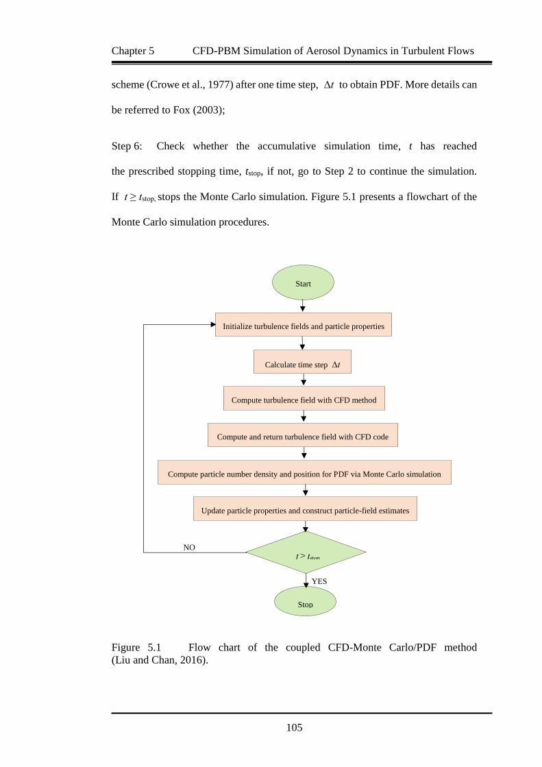
Chapter 5 CFD-PBM Simulation of Aerosol Dynamics in Turbulent Flows
105
scheme (Crowe et al., 1977) after one time step, ∆t to obtain PDF. More details can
be referred to Fox (2003);
Step 6: Check whether the accumulative simulation time, t has reached
the prescribed stopping time, tstop, if not, go to Step 2 to continue the simulation.
If t ≥ tstop, stops the Monte Carlo simulation. Figure 5.1 presents a flowchart of the
Monte Carlo simulation procedures.
Figure 5.1 Flow chart of the coupled CFD-Monte Carlo/PDF method
(Liu and Chan, 2016).
NO
YES
Start
Initialize turbulence fields and particle properties
Calculate time step ∆t
Compute turbulence field with CFD method
Compute and return turbulence field with CFD code
Compute particle number density and position for PDF via Monte Carlo simulation
Update particle properties and construct particle-field estimates
t ≥ tstop
Stop

Chapter 5 CFD-PBM Simulation of Aerosol Dynamics in Turbulent Flows
106
5.2.4 Simulation Analysis
Maximum relative error, ε and convergence time are used to show
the computational accuracy and efficiency. The definition of the maximum relative
error, max is written as:
max = {√[(n n0)
n0⁄ ]2} max (5-21)
where n is the particle number density obtained via CFD-MC method and n0 is
the particle number density obtained via the PBSM method based on the work of
Hounslow (1988). ε is the maximum relative error taken over the whole PSD
obtained via the above-mentioned two methods. Convergence time is defined as
the time needed for the physical quantities to reach the convergence criteria (1105)
with the proposed CFD-MC method. Normalized convergence time is defined as
the ratio of any convergence time to the shortest convergence time (i.e., the
convergence time of turbulent coagulation with Rej of 3200) in the present study.
The developed PBE (Hounslow, 1988) is used together with a dimensional
splitting technique (Ma et al., 2002) to formulate the PBSM method in this
Chapter 5 which makes the method applicable to multi-dimensional PBE.
Although the method of Hounslow (1988) is for a homogeneous PBE, it can be
modified to be applicable to multi-dimensional cases in the present study.
The specific method is to apply the one-dimensional high-resolution algorithm to
each one-dimensional homogeneous PBE (Equation 5-22) by setting the velocities
to be zero except for one certain coordinate sequentially at each time step (Gunawan
et al., 2004):

Chapter 5 CFD-PBM Simulation of Aerosol Dynamics in Turbulent Flows
107
∂f
∂t+ ∑
∂(Mj(L)f)
∂Lj = 0
n
j=1
where Mj is the rate of certain aerosol dynamic process, Lj is the internal coordinate
including spatial coordinate, j is the number of internal coordinates.
In order to analyze the variation of particle number density along the axial
distance, the particle number density is sampled at different evenly distributed
positions in the axial direction with the interval of 0.125 m, which is then plotted
versus axial distances. The normalized particle number density is defined as the ratio
of local particle number density to the particle number density at the outlet of the
nozzle as follows:
Nn =Nl
N0
where Nn is the normalized particle number density, Nl is the local particle number
density in the computational domain and N0 is the particle number density at the
outlet of the nozzle.
5.3 Simulation Setup
The configuration of the aerosol reactor in the present study is shown in
Figure 5.2. The aerosol reactor is a cylindrical aerosol reactor with radius of
0.225 m and length of 2 m. A nozzle with radius of 0.005m and length of 0.01 m is
located at the center of the cylindrical aerosol reactor. Three internals with height of
0.05 m and thickness of 0.0005 m are evenly mounted in the axial direction inside
cylindrical aerosol reactor in order to enhance mixing. For aerosol dynamics in
(5-22)
(5-23)

Chapter 5 CFD-PBM Simulation of Aerosol Dynamics in Turbulent Flows
108
turbulent flows, particles with a volume fraction of 0.1 in the carrier gas (air) is
injected from the nozzle while gas phase (air) is injected through the gas phase inlet.
The injected particles are potassium chloride (KCl) particles with a size range of
0.1 μm to 6.4 μm and density of 1980 kg/m3 (Calvo et al., 2013). The injection
velocity of particulate phase ranges from 10 m/s to 40 m/s, the inlet velocity of gas
phase is 0.5 m/s. Coagulation kernel is obtained using the turbulent coagulation
model by Saffman and Turner (1956). The nucleation rate is kept constant at
7.510−6 m-3s−1 with constant growth rate of 6.210−11 m/s. Aerosol dynamics in
laminar flow is also investigated in the same aerosol reactor for comparison with
aerosol dynamics in turbulent flows, which is carried out by switching the inlet
conditions of velocity and species between inlets of the nozzle and the gas phase.
The Reynolds number Rej of particulate phase is 1440 in the laminar flow. In the
turbulent flow, particles are injected from the nozzle of the aerosol reactor at 10 m/s
as shown in Figure 5.2. However, in the laminar flow, particles are injected through
the air inlet at 0.1m/s. Although the velocity of the jet in turbulent flow (10 m/s) is
higher than that of laminar flow (0.1 m/s), the cross-sectional area of the entrance
for particles in laminar flow (i.e., the cross-sectional area of the aerosol reactor with
a diameter of 0.225 m) is much higher than that for turbulent flow (i.e., the cross-
sectional area of the nozzle with a diameter of 0.005 m). Thus, the volume flowrate
for laminar flow is much higher than that for turbulent flow in the present study,
which is shown as follows:
Qlaminar = 20.25Qturbulent
where Qlaminar and Qturbulent are the volumetric flow rates of laminar flow and
turbulent flow, respectively. So the result of laminar flow in Figure 5.5 is scaled
(5-24)

Chapter 5 CFD-PBM Simulation of Aerosol Dynamics in Turbulent Flows
109
down to be consistent with the volumetric flow rate of the turbulent flow.
Specifically, for the study of aerosol dynamics in the laminar flow, particles enter
the gas phase inlet instead of the nozzle as shown in Figure 5.2 while the nozzle is
used for the entry of air at a low velocity of 0.5 m/s.
Figure 5.2 Three-dimensional schematic configuration of a cylindrical aerosol
reactor (Two-dimensional axisymmetric grid is generated in the rectangular domain
ABDC, not in scale) (Liu and Chan, 2016).
Due to the axisymmertrical configuration of the studied cylindrical aerosol
reactor, a two-dimensional axisymmetric unstructured grid corresponding to
the aerosol reactor is treated as shown in Figure 5.3. There are totally 8112 cells and
8444 nodes in the grid. The grid near the nozzle zone and internals is refined. Four
injection velocities of particulate phase i.e., 10 m/s, 15 m/s, 20 m/s and 40 m/s are
used to investigate the effect of jet Reynolds (Rej) number on the aerosol dynamics
in turbulent flows. Temperature is kept at 300 K for all the computational domain.
The standard k-ε turbulence model is used for the turbulence computation.
After balancing the computational accuracy and cost (i.e., computational time,
computer memory etc.), 30 notional particles are allocated in each cell in the present
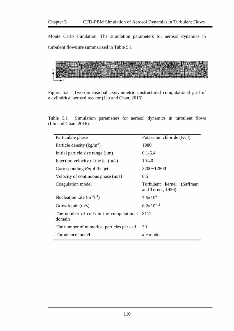
Chapter 5 CFD-PBM Simulation of Aerosol Dynamics in Turbulent Flows
110
Monte Carlo simulation. The simulation parameters for aerosol dynamics in
turbulent flows are summarized in Table 5.1
Figure 5.3 Two-dimensional axisymmetric unstructured computational grid of
a cylindrical aerosol reactor (Liu and Chan, 2016).
Table 5.1 Simulation parameters for aerosol dynamics in turbulent flows
(Liu and Chan, 2016).
Particulate phase Potassium chloride (KCl)
Particle density (kg/m3) 1980
Initial particle size range (μm) 0.1-6.4
Injection velocity of the jet (m/s) 10-40
Corresponding Rej of the jet 3200−12800
Velocity of continuous phase (m/s) 0.5
Coagulation model Turbulent kernel (Saffman
and Turner, 1956)
Nucleation rate (m-3s-1) 7.5106
Growth rate (m/s) 6.210−11
The number of cells in the computational
domain
8112
The number of numerical particles per cell 30
Turbulence model k-ε model

Chapter 5 CFD-PBM Simulation of Aerosol Dynamics in Turbulent Flows
111
5.4 Results and Discussion
5.4.1 Comparison of Coagulation in Both Laminar and Turbulent Flows
As mentioned above in Section 5.3, the inlet of fluid and particulate phases
is switched to simulate laminar flow, i.e., the particles are injected into the aerosol
reactor through the air inlet while air is injected through the nozzle (as shown in
Figure 5.2). The Rej number at the nozzle is 3200 with the injection velocity of
10 m/s for turbulent flows. The entry velocity of the gas phase (air) is 0.5 m/s for
both cases.
Figure 5.4 shows the initial PSD of particles before entering the aerosol
reactor. It can be seen that small particles account for the majority of the total particle
population. Figure 5.5 shows the PSD for particles after coagulation in both laminar
and turbulent flows. Compared with the PSD in Figure 5.4, it can be seen that
the PSD in Figure 5.5 varies significantly in its shape and order of magnitude
(decreasing the order of magnitude from 1019 to 1016) due to coagulation.
Coagulation is obviously enhanced in turbulent flows which can be seen from the
wider spectrum of PSD and higher maxima of particle number density when
compared to that in laminar flow. This is because coagulation in an inter-particle
process is dependent on the concentration and the mixing effect of particles.
Enhanced coagulation leads to a higher particle number density of particles with
diameter of 0.6 μm. As coagulation is only enhanced but the coagulation mechanism
is not changed, the peaks of the PSDs for laminar coagulation and turbulent
coagulation in Figure 5.5 appear in the same particle size.
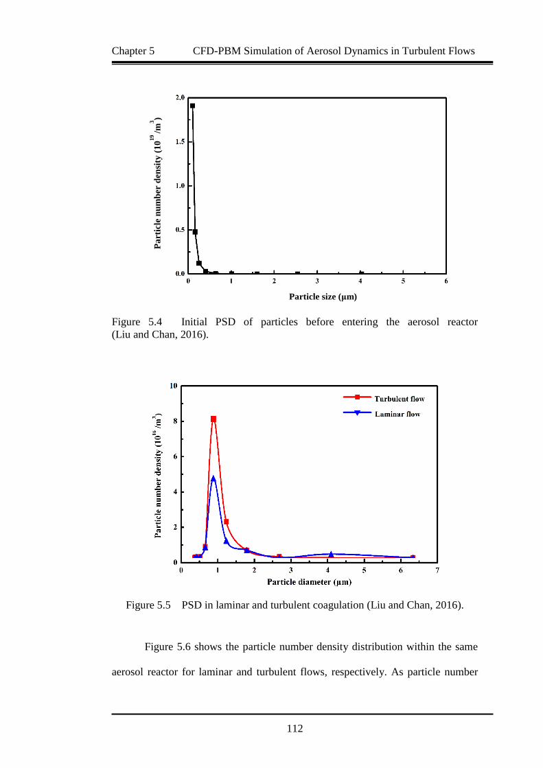
Chapter 5 CFD-PBM Simulation of Aerosol Dynamics in Turbulent Flows
112
Figure 5.4 Initial PSD of particles before entering the aerosol reactor
(Liu and Chan, 2016).
Figure 5.5 PSD in laminar and turbulent coagulation (Liu and Chan, 2016).
Figure 5.6 shows the particle number density distribution within the same
aerosol reactor for laminar and turbulent flows, respectively. As particle number
Pa
rtic
le n
um
ber
den
sity
(1
019 /m
3)
Particle size (μm)
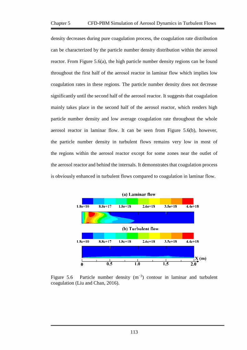
Chapter 5 CFD-PBM Simulation of Aerosol Dynamics in Turbulent Flows
113
density decreases during pure coagulation process, the coagulation rate distribution
can be characterized by the particle number density distribution within the aerosol
reactor. From Figure 5.6(a), the high particle number density regions can be found
throughout the first half of the aerosol reactor in laminar flow which implies low
coagulation rates in these regions. The particle number density does not decrease
significantly until the second half of the aerosol reactor. It suggests that coagulation
mainly takes place in the second half of the aerosol reactor, which renders high
particle number density and low average coagulation rate throughout the whole
aerosol reactor in laminar flow. It can be seen from Figure 5.6(b), however,
the particle number density in turbulent flows remains very low in most of
the regions within the aerosol reactor except for some zones near the outlet of
the aerosol reactor and behind the internals. It demonstrates that coagulation process
is obviously enhanced in turbulent flows compared to coagulation in laminar flow.
Figure 5.6 Particle number density (m−3) contour in laminar and turbulent
coagulation (Liu and Chan, 2016).

Chapter 5 CFD-PBM Simulation of Aerosol Dynamics in Turbulent Flows
114
5.4.2 The Effect of Rej Number on Coagulation in Turbulent Flows
The enhanced effect of turbulence on coagulation is shown in Section 5.4.1.
The effect of different Rej numbers on coagulation process in turbulent flows is
further studied. Varied jet velocities of 10 m/s, 15 m/s, 20 m/s and 40 m/s are used
with corresponding Re numbers of 3200, 4800, 6400 and 12800, respectively.
The results obtained via the proposed Lagrangian Monte Carlo/PDF (LMC-PDF)
method are directly compared with those obtained via the modified population
balance sectional method (PBSM) (Hounslow, 1988).
Figure 5.7 PSD in turbulent coagulation: Case A, Rej = 3200; Case B, Rej =4800;
Case C, Rej = 6400; Case D, Rej =12800 (The PBSM results are obtained based on
the method proposed by Hounslow (1988)) (Liu and Chan, 2016).
Figure 5.7 shows the obvious effect of different Rej numbers on the PSD of
aerosol particles experiencing coagulation process in turbulent flows. With Re
number of the jet increasing from 3200 to 12800, the PSDs become wider and higher,
with the peaks moving towards the larger end of particle size range, which yields a
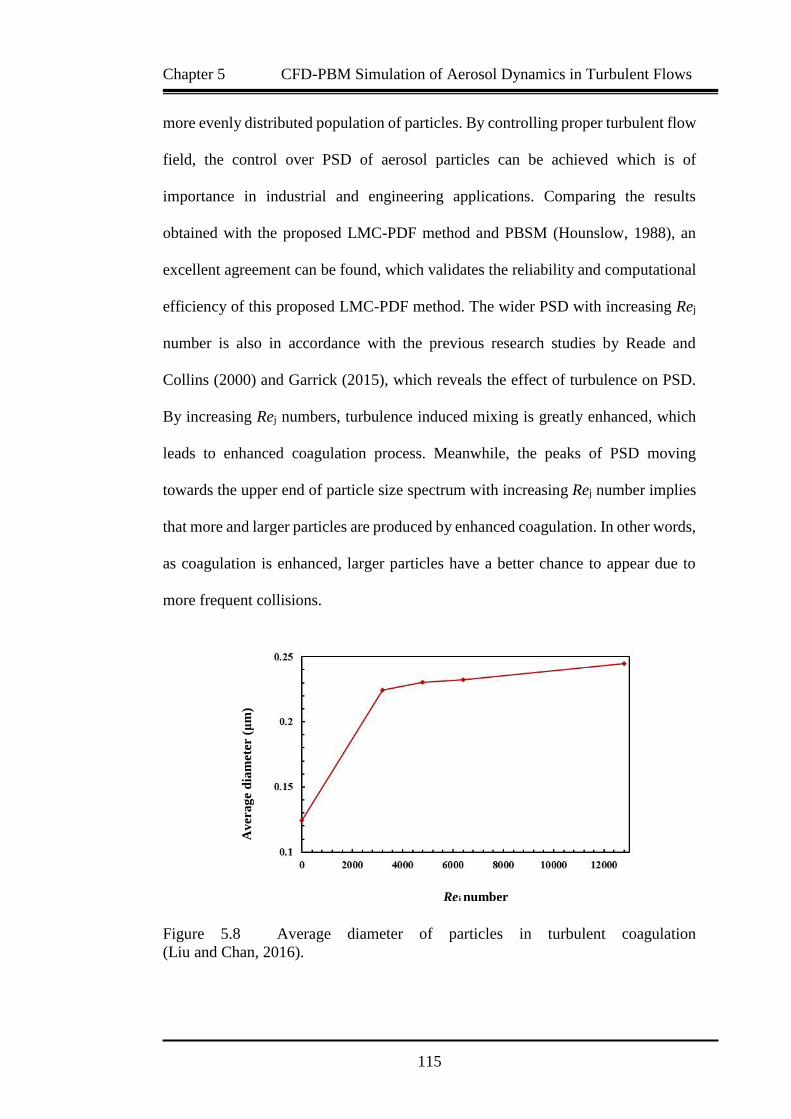
Chapter 5 CFD-PBM Simulation of Aerosol Dynamics in Turbulent Flows
115
more evenly distributed population of particles. By controlling proper turbulent flow
field, the control over PSD of aerosol particles can be achieved which is of
importance in industrial and engineering applications. Comparing the results
obtained with the proposed LMC-PDF method and PBSM (Hounslow, 1988), an
excellent agreement can be found, which validates the reliability and computational
efficiency of this proposed LMC-PDF method. The wider PSD with increasing Rej
number is also in accordance with the previous research studies by Reade and
Collins (2000) and Garrick (2015), which reveals the effect of turbulence on PSD.
By increasing Rej numbers, turbulence induced mixing is greatly enhanced, which
leads to enhanced coagulation process. Meanwhile, the peaks of PSD moving
towards the upper end of particle size spectrum with increasing Rej number implies
that more and larger particles are produced by enhanced coagulation. In other words,
as coagulation is enhanced, larger particles have a better chance to appear due to
more frequent collisions.
Figure 5.8 Average diameter of particles in turbulent coagulation
(Liu and Chan, 2016).
Rej number
Av
era
ge
dia
met
er (
μm
)

Chapter 5 CFD-PBM Simulation of Aerosol Dynamics in Turbulent Flows
116
According to the definition of particle number based on average diameter of
particles (Friedlander, 2000), the number averaged particle diameter can be obtained
by integrating the PSD over the entire particle diameter range and then averaging
over the total particle number density of particles. Using this method, the initial
average diameter and average diameters of particles under the turbulent coagulation
for different Rej numbers are obtained and shown in Figure 5.8. An increase in
average diameter from 0.124 μm to 0.245 μm can be observed with increasing Rej
number from 0 to 12800, which is an obvious increase considering the large number
of aerosol particles in the aerosol reactor. The Rej number of zero corresponds to
the initial PSD of aerosol dynamics before entering the aerosol reactor. As higher
Reynold number of the jet is related to higher turbulent intensity in the present study,
the increase of average particle diameter with Rej number indicates that coagulation
is significantly enhanced, which may be explained by the enhanced mixing and more
frequent collisions between particles.
The turbulent kinetic energy (m2/s2) under different Rej numbers is presented
in Figures 5.9(a) to (d). As the length of aerosol reactor is 2 m, which is much longer
than the nozzle whose length is only 0.01 m, the turbulent zones directly caused by
the injection of particulate phase are quite limited as shown in Figure 5.9.
The maximum axial length is around 0.5 m (determined from the first internal in
the aerosol reactor) and the maximum radial length is around 0.05 m, which is less
than a quarter of the radius of the aerosol reactor. With the increasing Rej number,
the turbulent kinetic energy (m2/s2) also increases according to Figure 5.9.
However, the results presented in Figure 5.7 indicate that turbulence has significant
impact on coagulation process in turbulent flows despite of the limited zones of
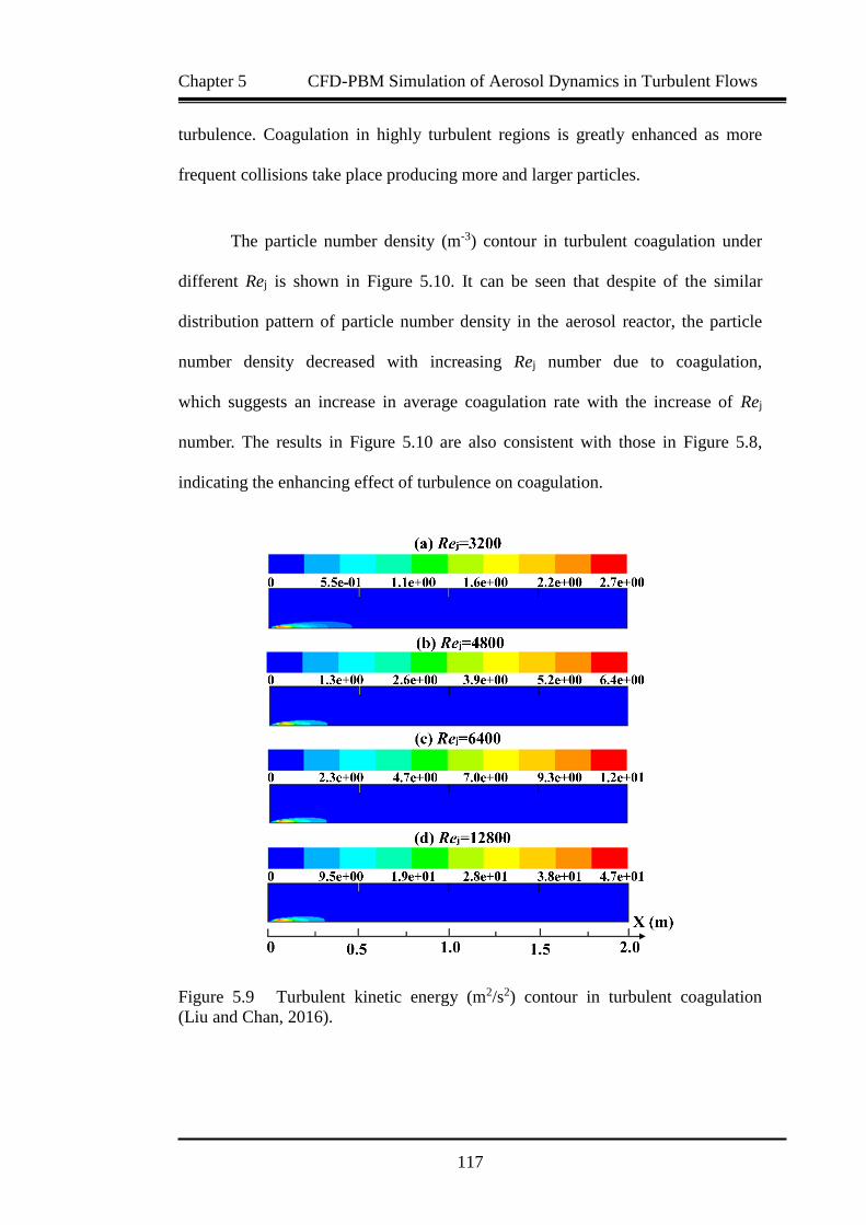
Chapter 5 CFD-PBM Simulation of Aerosol Dynamics in Turbulent Flows
117
turbulence. Coagulation in highly turbulent regions is greatly enhanced as more
frequent collisions take place producing more and larger particles.
The particle number density (m-3) contour in turbulent coagulation under
different Rej is shown in Figure 5.10. It can be seen that despite of the similar
distribution pattern of particle number density in the aerosol reactor, the particle
number density decreased with increasing Rej number due to coagulation,
which suggests an increase in average coagulation rate with the increase of Rej
number. The results in Figure 5.10 are also consistent with those in Figure 5.8,
indicating the enhancing effect of turbulence on coagulation.
Figure 5.9 Turbulent kinetic energy (m2/s2) contour in turbulent coagulation
(Liu and Chan, 2016).

Chapter 5 CFD-PBM Simulation of Aerosol Dynamics in Turbulent Flows
118
Figure 5.10 Particle number density (m−3) contour in turbulent coagulation
(Liu and Chan, 2016).
Figure 5.11 shows the variation of normalized particle number density with
the axial distance under different Rej. As coagulation process continuously reduces
particle number density, it can be seen that the normalized particle number density
for any fixed Rej decreases with the axial distance as coagulation process takes place.
Consider the same axial position, the difference between the normalized particle
number density shows the different coagulation rates. Obviously, a higher Rej yields
higher turbulence, which in turn leads to a higher coagulation rate. The results in
Figure 5.11 show clearly the enhancing effect of turbulence on coagulation.
When Rej reaches 12800, the maximum value used in the present study, it can be
observed that the normalized particle number density first decreases rapidly, then
decreases slightly and finally decreases with the rate almost equal to that with Rej of

Chapter 5 CFD-PBM Simulation of Aerosol Dynamics in Turbulent Flows
119
6400. The three-stage decrease of normalized particle number density indicates
that the coagulation rate experiences with three different stages. This may be
explained by the physical nature of coagulation process. Coagulation is a binary
particle event which is dependent on local concentration and micro-mixing.
Coagulation rate is first increased due to the enhanced mixing caused by high
turbulence, which consumes a large number of particles in a short time. As a result,
a low local concentration of particles in turn reduces the coagulation rate until more
particles are accumulated and coagulation rate increases again in the final stage.
Figure 5.11 Normalized particle number density of turbulent coagulation
(Liu and Chan, 2016).
5.4.3 The Effect of Rej Number on Coagulation and Nucleation in Turbulent
Flows
The effect of different Rej numbers on two simultaneous aerosol dynamic
processes (i.e., coagulation and nucleation) in turbulent flows is studied.
The adopted Rej numbers are the same as described before. Coagulation process is
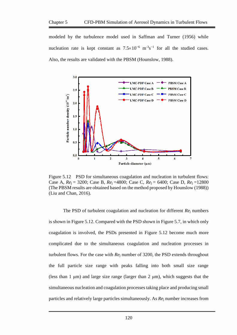
Chapter 5 CFD-PBM Simulation of Aerosol Dynamics in Turbulent Flows
120
modeled by the turbulence model used in Saffman and Turner (1956) while
nucleation rate is kept constant as 7.510−6 m-3s−1 for all the studied cases.
Also, the results are validated with the PBSM (Hounslow, 1988).
Figure 5.12 PSD for simultaneous coagulation and nucleation in turbulent flows:
Case A, Rej = 3200; Case B, Rej =4800; Case C, Rej = 6400; Case D, Rej =12800
(The PBSM results are obtained based on the method proposed by Hounslow (1988))
(Liu and Chan, 2016).
The PSD of turbulent coagulation and nucleation for different Rej numbers
is shown in Figure 5.12. Compared with the PSD shown in Figure 5.7, in which only
coagulation is involved, the PSDs presented in Figure 5.12 become much more
complicated due to the simultaneous coagulation and nucleation processes in
turbulent flows. For the case with Rej number of 3200, the PSD extends throughout
the full particle size range with peaks falling into both small size range
(less than 1 μm) and large size range (larger than 2 μm), which suggests that the
simultaneous nucleation and coagulation processes taking place and producing small
particles and relatively large particles simultaneously. As Rej number increases from
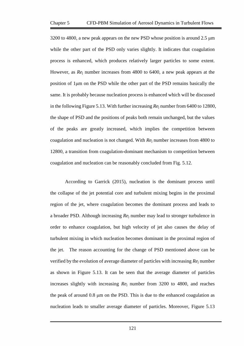
Chapter 5 CFD-PBM Simulation of Aerosol Dynamics in Turbulent Flows
121
3200 to 4800, a new peak appears on the new PSD whose position is around 2.5 μm
while the other part of the PSD only varies slightly. It indicates that coagulation
process is enhanced, which produces relatively larger particles to some extent.
However, as Rej number increases from 4800 to 6400, a new peak appears at the
position of 1μm on the PSD while the other part of the PSD remains basically the
same. It is probably because nucleation process is enhanced which will be discussed
in the following Figure 5.13. With further increasing Rej number from 6400 to 12800,
the shape of PSD and the positions of peaks both remain unchanged, but the values
of the peaks are greatly increased, which implies the competition between
coagulation and nucleation is not changed. With Rej number increases from 4800 to
12800, a transition from coagulation-dominant mechanism to competition between
coagulation and nucleation can be reasonably concluded from Fig. 5.12.
According to Garrick (2015), nucleation is the dominant process until
the collapse of the jet potential core and turbulent mixing begins in the proximal
region of the jet, where coagulation becomes the dominant process and leads to
a broader PSD. Although increasing Rej number may lead to stronger turbulence in
order to enhance coagulation, but high velocity of jet also causes the delay of
turbulent mixing in which nucleation becomes dominant in the proximal region of
the jet. The reason accounting for the change of PSD mentioned above can be
verified by the evolution of average diameter of particles with increasing Rej number
as shown in Figure 5.13. It can be seen that the average diameter of particles
increases slightly with increasing Rej number from 3200 to 4800, and reaches
the peak of around 0.8 μm on the PSD. This is due to the enhanced coagulation as
nucleation leads to smaller average diameter of particles. Moreover, Figure 5.13
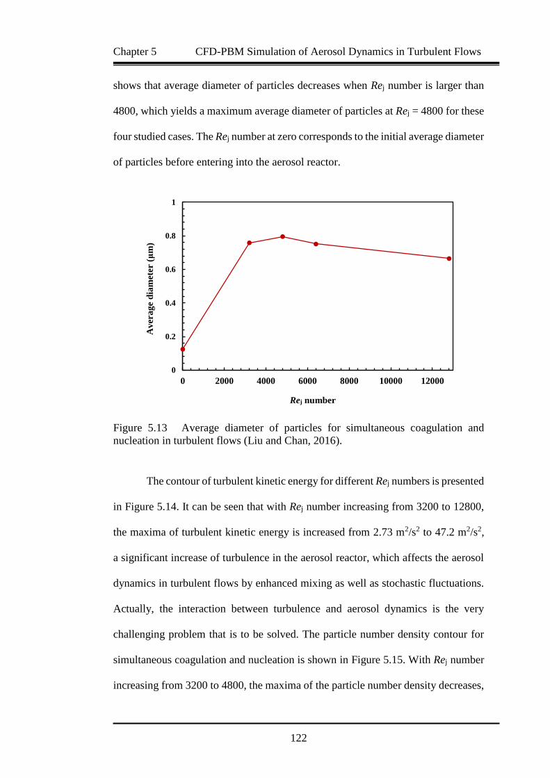
Chapter 5 CFD-PBM Simulation of Aerosol Dynamics in Turbulent Flows
122
shows that average diameter of particles decreases when Rej number is larger than
4800, which yields a maximum average diameter of particles at Rej = 4800 for these
four studied cases. The Rej number at zero corresponds to the initial average diameter
of particles before entering into the aerosol reactor.
Figure 5.13 Average diameter of particles for simultaneous coagulation and
nucleation in turbulent flows (Liu and Chan, 2016).
The contour of turbulent kinetic energy for different Rej numbers is presented
in Figure 5.14. It can be seen that with Rej number increasing from 3200 to 12800,
the maxima of turbulent kinetic energy is increased from 2.73 m2/s2 to 47.2 m2/s2,
a significant increase of turbulence in the aerosol reactor, which affects the aerosol
dynamics in turbulent flows by enhanced mixing as well as stochastic fluctuations.
Actually, the interaction between turbulence and aerosol dynamics is the very
challenging problem that is to be solved. The particle number density contour for
simultaneous coagulation and nucleation is shown in Figure 5.15. With Rej number
increasing from 3200 to 4800, the maxima of the particle number density decreases,
0
0.2
0.4
0.6
0.8
1
0 2000 4000 6000 8000 10000 12000
Rej number
Av
era
ge
dia
met
er (
μm
)

Chapter 5 CFD-PBM Simulation of Aerosol Dynamics in Turbulent Flows
123
implying that coagulation process which reduces particle density is dominant. An
increase of the maxima of particle number density is observed when Rej number
increases from 4800 to 12800.
Figure 5.14 Turbulent kinetic energy (m2/s2) contour for simultaneous coagulation
and nucleation in turbulent flows (Liu and Chan, 2016).
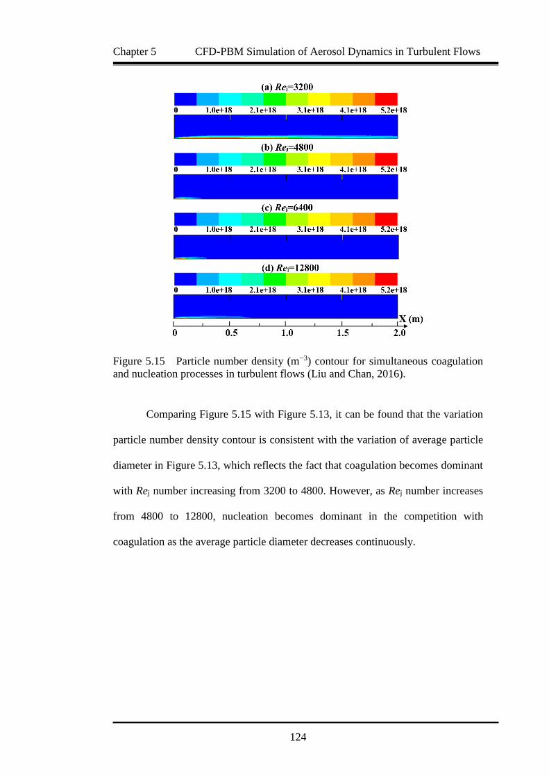
Chapter 5 CFD-PBM Simulation of Aerosol Dynamics in Turbulent Flows
124
Figure 5.15 Particle number density (m−3) contour for simultaneous coagulation
and nucleation processes in turbulent flows (Liu and Chan, 2016).
Comparing Figure 5.15 with Figure 5.13, it can be found that the variation
particle number density contour is consistent with the variation of average particle
diameter in Figure 5.13, which reflects the fact that coagulation becomes dominant
with Rej number increasing from 3200 to 4800. However, as Rej number increases
from 4800 to 12800, nucleation becomes dominant in the competition with
coagulation as the average particle diameter decreases continuously.
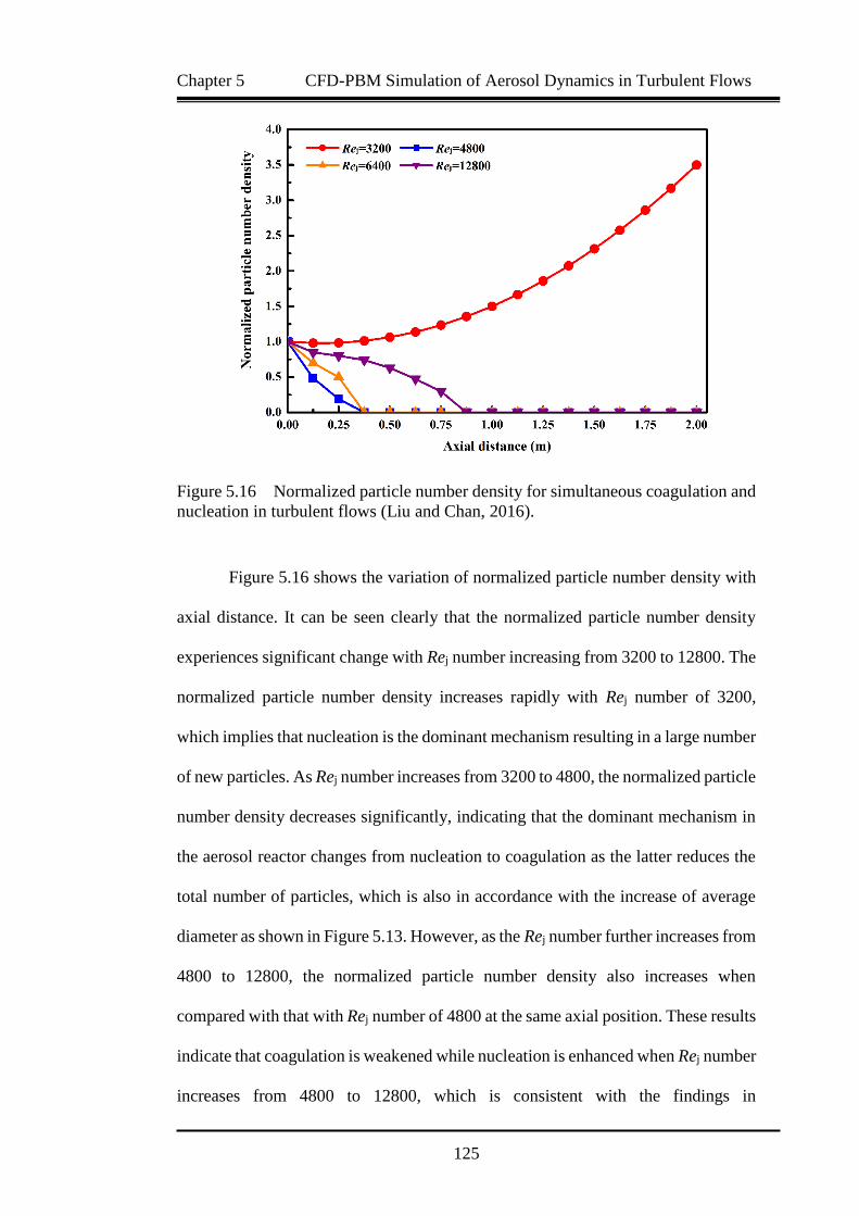
Chapter 5 CFD-PBM Simulation of Aerosol Dynamics in Turbulent Flows
125
Figure 5.16 Normalized particle number density for simultaneous coagulation and
nucleation in turbulent flows (Liu and Chan, 2016).
Figure 5.16 shows the variation of normalized particle number density with
axial distance. It can be seen clearly that the normalized particle number density
experiences significant change with Rej number increasing from 3200 to 12800. The
normalized particle number density increases rapidly with Rej number of 3200,
which implies that nucleation is the dominant mechanism resulting in a large number
of new particles. As Rej number increases from 3200 to 4800, the normalized particle
number density decreases significantly, indicating that the dominant mechanism in
the aerosol reactor changes from nucleation to coagulation as the latter reduces the
total number of particles, which is also in accordance with the increase of average
diameter as shown in Figure 5.13. However, as the Rej number further increases from
4800 to 12800, the normalized particle number density also increases when
compared with that with Rej number of 4800 at the same axial position. These results
indicate that coagulation is weakened while nucleation is enhanced when Rej number
increases from 4800 to 12800, which is consistent with the findings in
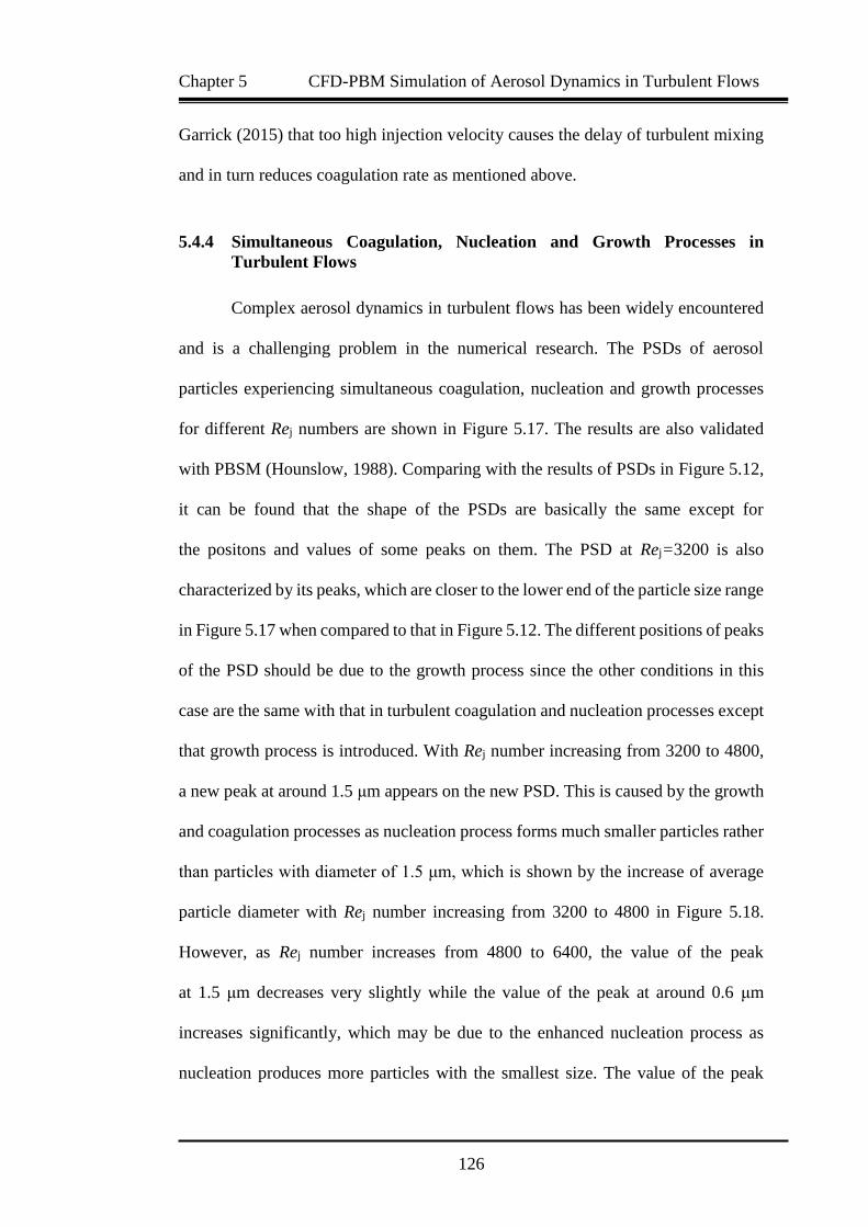
Chapter 5 CFD-PBM Simulation of Aerosol Dynamics in Turbulent Flows
126
Garrick (2015) that too high injection velocity causes the delay of turbulent mixing
and in turn reduces coagulation rate as mentioned above.
5.4.4 Simultaneous Coagulation, Nucleation and Growth Processes in
Turbulent Flows
Complex aerosol dynamics in turbulent flows has been widely encountered
and is a challenging problem in the numerical research. The PSDs of aerosol
particles experiencing simultaneous coagulation, nucleation and growth processes
for different Rej numbers are shown in Figure 5.17. The results are also validated
with PBSM (Hounslow, 1988). Comparing with the results of PSDs in Figure 5.12,
it can be found that the shape of the PSDs are basically the same except for
the positons and values of some peaks on them. The PSD at Rej=3200 is also
characterized by its peaks, which are closer to the lower end of the particle size range
in Figure 5.17 when compared to that in Figure 5.12. The different positions of peaks
of the PSD should be due to the growth process since the other conditions in this
case are the same with that in turbulent coagulation and nucleation processes except
that growth process is introduced. With Rej number increasing from 3200 to 4800,
a new peak at around 1.5 μm appears on the new PSD. This is caused by the growth
and coagulation processes as nucleation process forms much smaller particles rather
than particles with diameter of 1.5 μm, which is shown by the increase of average
particle diameter with Rej number increasing from 3200 to 4800 in Figure 5.18.
However, as Rej number increases from 4800 to 6400, the value of the peak
at 1.5 μm decreases very slightly while the value of the peak at around 0.6 μm
increases significantly, which may be due to the enhanced nucleation process as
nucleation produces more particles with the smallest size. The value of the peak
Chapter 5 CFD-PBM Simulation of Aerosol Dynamics in Turbulent Flows
127
at 0.6 μm increased sharply again with Rej number increasing from 6400 to 12800,
implying that nucleation process is further enhanced to be the dominant process.
Figure 5.17 PSD for simultaneous coagulation, nucleation and growth in turbulent
flows: Case A, Rej = 3200; Case B, Rej =4800; Case C, Rej = 6400; Case D,
Rej =12800 (The PBSM results are obtained based on the method proposed by
Hounslow (1988)) (Liu and Chan, 2016).
The average diameters of particles for different Rej numbers are calculated
in order to reveal the physical mechanism behind the change of the PSD. Figure 5.18
shows an increase in average diameter of particles for increasing Rej number from
3200 to 4800. Whereas for Rej number larger than 4800 (within these four studied
Rej numbers for this case), the average diameter of particles decreases with
increasing Rej number. Based on the average diameter of particles calculated from
the obtained PSD, it can be concluded that, with increasing Rej number from 4800
to 6400, the change of the peak at around 0.6 μm is due to pure nucleation as neither
growth nor coagulation leads to the decrease in average diameter of particles.
Comparing the case of turbulent coagulation and nucleation processes in Figure 5.13
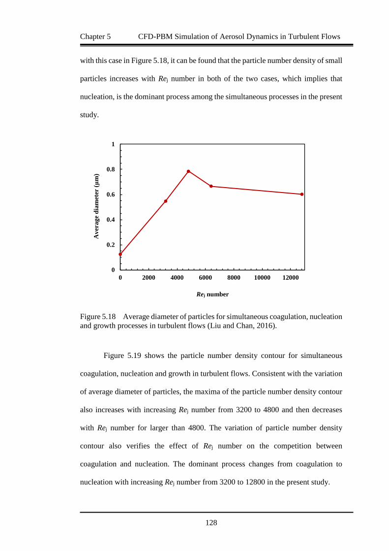
Chapter 5 CFD-PBM Simulation of Aerosol Dynamics in Turbulent Flows
128
with this case in Figure 5.18, it can be found that the particle number density of small
particles increases with Rej number in both of the two cases, which implies that
nucleation, is the dominant process among the simultaneous processes in the present
study.
Figure 5.18 Average diameter of particles for simultaneous coagulation, nucleation
and growth processes in turbulent flows (Liu and Chan, 2016).
Figure 5.19 shows the particle number density contour for simultaneous
coagulation, nucleation and growth in turbulent flows. Consistent with the variation
of average diameter of particles, the maxima of the particle number density contour
also increases with increasing Rej number from 3200 to 4800 and then decreases
with Rej number for larger than 4800. The variation of particle number density
contour also verifies the effect of Rej number on the competition between
coagulation and nucleation. The dominant process changes from coagulation to
nucleation with increasing Rej number from 3200 to 12800 in the present study.
0
0.2
0.4
0.6
0.8
1
0 2000 4000 6000 8000 10000 12000
Av
era
ge
dia
met
er (
μm
)
Rej number
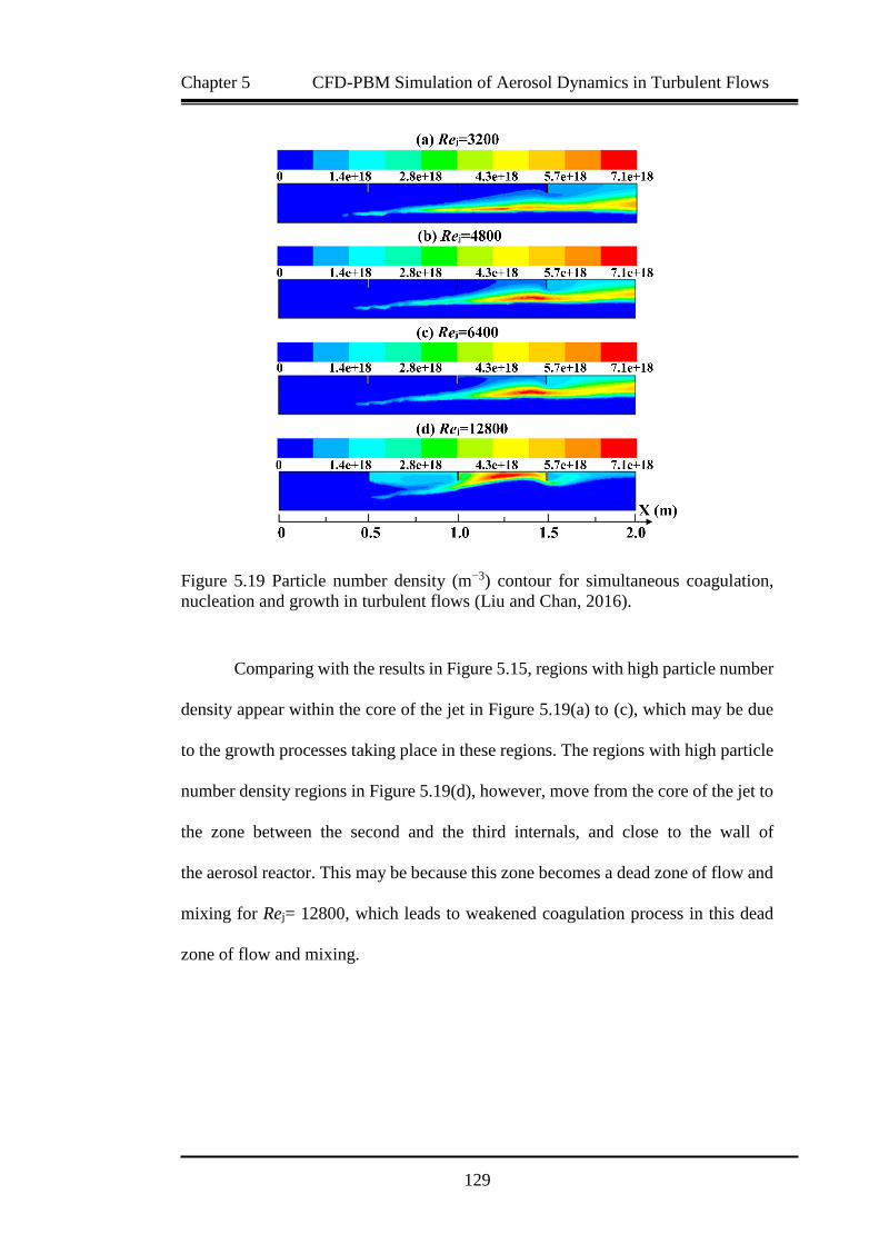
Chapter 5 CFD-PBM Simulation of Aerosol Dynamics in Turbulent Flows
129
Figure 5.19 Particle number density (m−3) contour for simultaneous coagulation,
nucleation and growth in turbulent flows (Liu and Chan, 2016).
Comparing with the results in Figure 5.15, regions with high particle number
density appear within the core of the jet in Figure 5.19(a) to (c), which may be due
to the growth processes taking place in these regions. The regions with high particle
number density regions in Figure 5.19(d), however, move from the core of the jet to
the zone between the second and the third internals, and close to the wall of
the aerosol reactor. This may be because this zone becomes a dead zone of flow and
mixing for Rej= 12800, which leads to weakened coagulation process in this dead
zone of flow and mixing.
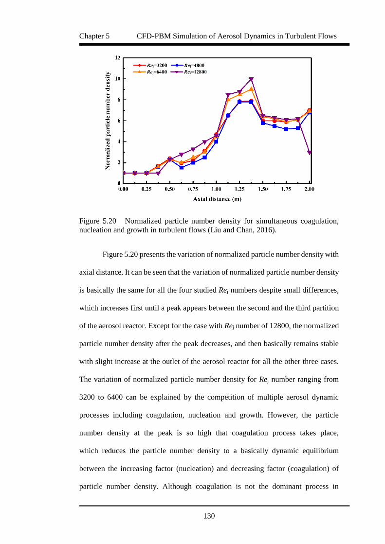
Chapter 5 CFD-PBM Simulation of Aerosol Dynamics in Turbulent Flows
130
Figure 5.20 Normalized particle number density for simultaneous coagulation,
nucleation and growth in turbulent flows (Liu and Chan, 2016).
Figure 5.20 presents the variation of normalized particle number density with
axial distance. It can be seen that the variation of normalized particle number density
is basically the same for all the four studied Rej numbers despite small differences,
which increases first until a peak appears between the second and the third partition
of the aerosol reactor. Except for the case with Rej number of 12800, the normalized
particle number density after the peak decreases, and then basically remains stable
with slight increase at the outlet of the aerosol reactor for all the other three cases.
The variation of normalized particle number density for Rej number ranging from
3200 to 6400 can be explained by the competition of multiple aerosol dynamic
processes including coagulation, nucleation and growth. However, the particle
number density at the peak is so high that coagulation process takes place,
which reduces the particle number density to a basically dynamic equilibrium
between the increasing factor (nucleation) and decreasing factor (coagulation) of
particle number density. Although coagulation is not the dominant process in
Chapter 5 CFD-PBM Simulation of Aerosol Dynamics in Turbulent Flows
131
the four studied cases, it is still shown in Fig. 5.20 that once the Rej number is larger
than 4800, the normalized particle number density increases due to the delay of
turbulent mixing at high injection velocity (Garrick, 2015). As for the case with Rej
number of 12800, the low particle number density near the outlet of the aerosol
reactor may be caused by the dead zone between the second and the third partitions
of the aerosol reactor where those particles are trapped.
5.4.5 Computational Accuracy and Efficiency
The term “accuracy” here refers to the agreement between the numerical
simulation results via the proposed coupled CFD-Monte Carlo method and the
reference method (i.e. the PBSM method). The maximum relative error and
normalized convergence time for different studied cases are shown in Table 5.2. It
can be seen that for the same Rej number, the maximum relative error only varies
very slightly for different aerosol dynamic processes. With the Rej number
increasing from 3200 to 12800, however, the maximum relative error for any of the
studied cases in Table 5.2 increases rapidly, which may be explained by the
increasing turbulent fluctuations caused by the increasing Rej number. The
maximum relative error amongst all the studied cases is only 4.83%, which proves
the high accuracy of this newly proposed and developed CFD-MC method. The
normalized convergence time is used to represent the computational efficiency of
the numerical simulation. It can be seen that for any fixed case amongst the studied
cases in Table 5.2, the normalized convergence time only increases very slightly
with increasing Rej number. However, comparing different studied cases with the
same Rej number shows that the normalized convergence time increases
significantly with the complexity of the studied cases. When Rej number is 12800,

Chapter 5 CFD-PBM Simulation of Aerosol Dynamics in Turbulent Flows
132
for instance, the normalized convergence time of pure coagulation process is about
1.10, which increases to 5.00 for coagulation and nucleation processes and to 11.25
for simultaneous coagulation, nucleation and growth processes, respectively. The
variation of the normalized convergence time shows that the complexity of the
studied cases has much greater influence on the computational efficiency than Rej
number, which may be because more computational time is needed for more
complex aerosol dynamic processes in order to reach convergence. It can be also
seen that although PBSM method needs a shorter normalized convergence time than
the LMC-PDF method for the simple cases, almost the same normalized
convergence time is needed for complex cases. Thus, this newly proposed and
validated LMC-PDF provides an efficient but relatively simple algorithm.
Table 5.2 Maximum relative error and normalized convergence time for different
studied cases (Liu and Chan, 2016).
Studied
cases Rej
Maximum
relative error,
max (%)
Normalized
convergence time
of LMC-PDF
Normalized
convergence
time of PBSM
Coagulation
3200 1.00 1.00 0.75
4800 3.00 1.08 0.88
6400 4.10 1.08 0.88
12800 4.60 1.10 1.00
Coagulation
and
nucleation
3200 1.00 4.50 4.00
4800 2.90 4.50 4.00
6400 4.30 4.63 4.25
12800 4.80 5.00 5.00
Coagulation,
nucleation
and growth
3200 1.10 10.00 10.00
4800 3.00 10.25 10.25
6400 4.30 10.75 10.50
12800 4.80 11.25 11.25
LMC-PDF: Lagrangian Monte Carlo-PDF method; PBSM: Population balance
sectional method. The convergence time is normalized based on the ratio of any
convergence time to the shortest convergence (i.e., the convergence time of
turbulent coagulation for Rej = 3200) in the present study.

Chapter 5 CFD-PBM Simulation of Aerosol Dynamics in Turbulent Flows
133
5.4.6 Numerical Stability Analysis
The typical grid independence analysis is given in Table 5.3. For the
relatively simple turbulent coagulation case (Rej=3200), the normalized
convergence time increases to more than nine times (i.e., from 1.00 to 9.36) with the
number of grid cells increasing from 8112 to 22800 while the maximum relative
error hardly changes (i.e, from 1.00% to 0.99%). For the relatively complex
simultaneous case such as coagulation, nucleation and growth processes
(Rej = 12800), the normalized convergence time increases rapidly and drastically
(i.e., from 11.25 to 112.50) with number of grid cells increasing from 8112 to 22800
while the maximum relative error hardly changes (i.e., from 4.80% to 4.78%).
So the grid cell independence can be confirmed from Table 5.3 and the optimal grid
cells is selected to be 8112 in the present study.
Table 5.3 Typical grid cell independence analysis.
Selected cases Number of
grid cells
Maximum relative
error, max (%)
Normalized convergence
time
Turbulent
Coagulation
(Rej,= 3200)
8112
12044
15200
22800
1.00 1.00
0.99 2.25
0.99 4.00
0.99 9.36
Coagulation
nucleation and
growth
(Rej= 12800)
8112 4.80 11.25
12044 4.80 25.30
15200 4.79 45.00
22800 4.78 112.50
The normalized convergence time is defined by the ratio of any convergence
time to the shortest convergence (i.e., the convergence time of turbulent
coagulation for Rej = 3200) in the present study.
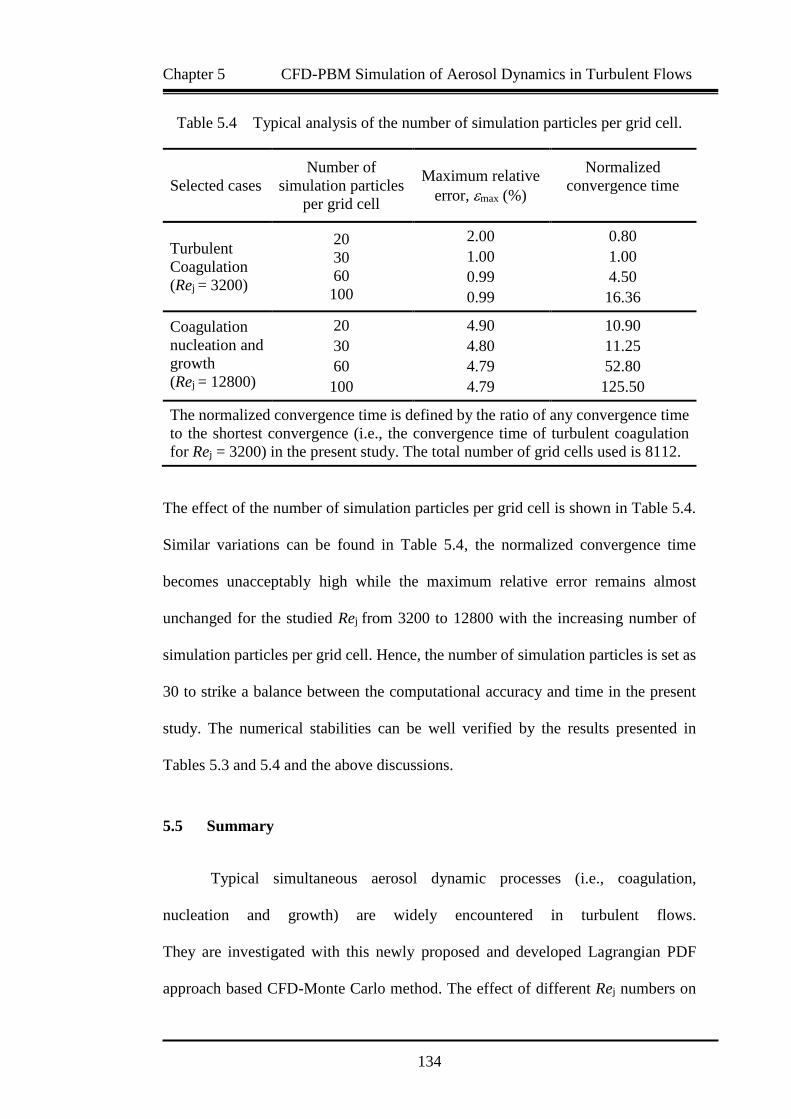
Chapter 5 CFD-PBM Simulation of Aerosol Dynamics in Turbulent Flows
134
Table 5.4 Typical analysis of the number of simulation particles per grid cell.
Selected cases
Number of
simulation particles
per grid cell
Maximum relative
error, max (%)
Normalized
convergence time
Turbulent
Coagulation
(Rej = 3200)
20
30
60
100
2.00 0.80
1.00 1.00
0.99 4.50
0.99 16.36
Coagulation
nucleation and
growth
(Rej = 12800)
20 4.90 10.90
30 4.80 11.25
60 4.79 52.80
100 4.79 125.50
The normalized convergence time is defined by the ratio of any convergence time
to the shortest convergence (i.e., the convergence time of turbulent coagulation
for Rej = 3200) in the present study. The total number of grid cells used is 8112.
The effect of the number of simulation particles per grid cell is shown in Table 5.4.
Similar variations can be found in Table 5.4, the normalized convergence time
becomes unacceptably high while the maximum relative error remains almost
unchanged for the studied Rej from 3200 to 12800 with the increasing number of
simulation particles per grid cell. Hence, the number of simulation particles is set as
30 to strike a balance between the computational accuracy and time in the present
study. The numerical stabilities can be well verified by the results presented in
Tables 5.3 and 5.4 and the above discussions.
5.5 Summary
Typical simultaneous aerosol dynamic processes (i.e., coagulation,
nucleation and growth) are widely encountered in turbulent flows.
They are investigated with this newly proposed and developed Lagrangian PDF
approach based CFD-Monte Carlo method. The effect of different Rej numbers on

Chapter 5 CFD-PBM Simulation of Aerosol Dynamics in Turbulent Flows
135
the interaction between turbulence and aerosol dynamics is fully studied.
The results reveal the significant impact of Rej on both single aerosol process (e.g.
coagulation) and the competitive and simultaneous aerosol dynamic processes in
turbulent flows.
This newly proposed and validated CFD-Monte Carlo/PDF method renders an
efficient and accurate method to deal with the interaction between turbulence and
aerosol dynamics by overcoming the closure problems. The full PSD of aerosol
particles is accurately obtained. The enhancing effect of turbulence on coagulation
is demonstrated by comparison of laminar coagulation and turbulent coagulation.
Further study reveals the effect of turbulence on the PSDs for simultaneous aerosol
dynamic processes and significant impact of turbulence on the final PSD of particles.
For simultaneous complex aerosol dynamics in turbulent flows, turbulence plays an
important role in broadening the PSD. The coupled CFD-Monte Carlo/PDF method
also shows excellent numerical stability according to typical grid cell independence
analysis and typical analysis of the number of simulation particles per grid cell.

Chapter 6 Simulation of Aerosol Dynamics in Turbulent Reactive Flows
136
Chapter 6 Simulation of Aerosol Dynamics in Turbulent
Reactive flows
6.1 Introduction
Combustion processes of the fossil fuels contain brief descriptions that
convert the chemical energy into sensible energy in the products.
The fossil fuels provide a major source of energy for miscellaneous applications
ranging from household and industrial heating to power generation and metallurgy
as well as combustion chamber in engine and propulsion systems
(Kuo and Acharya, 2012). Turbulent reactive flows conditions are widely
encountered in most practical combustion devices such as internal combustion (IC)
engine and fluidized bed. The release of chemical energy involves radiative heat
transfer (Modest, 2003) and pollutant emissions (Boushaki et al., 2016).
Models accounting for all aspects of combustion devices ranging from gas turbines
and IC engines to industrial furnaces are needed to meet the increasingly stricter
emissions regulations from combustion devices and the higher combustion
efficiency requirements. Thus, it is necessary to develop models with various
physical sub-processes and detailed chemistry in combustion process to evaluate the
performance of different combustion flows. Moreover, turbulence adds to the
complexity required for modeling of combustion processes resulting from the
turbulence chemistry interaction (TCI) and turbulence radiation interaction (TRI)
(Mehta, 2008). The modeling of soot formation in turbulent reactive flows is the
focus of this chapter.
A comprehensive modeling of turbulent reactive flows, including detailed
chemistry, radiation and soot models with detailed closures for TCI and TRI is

Chapter 6 Simulation of Aerosol Dynamics in Turbulent Reactive Flow
137
presented in this chapter. This newly proposed and validated CFD-MC method
(Liu and Chan, 2016) derived from the transported PDF approach coupling with PBE
in Chapter 5 is used to simulate a turbulent non-premixed jet flame of methane.
A time-dependent Reynolds-averaged Navier-Stokes (RANS) model is used in
conjunction with the k-ε turbulence model as the CFD code to solve the turbulent
combustion flow fields. One of the advantages of using the transported PDF
approach is that the chemical reaction source, radiation emission and soot generation
source terms appear in closed form (Akridis and Rigopoulos, 2015).
Both the kinetics of soot formation kinetics and the chemistry of combustion
are taken into account in the numerical simulation. The classical combustion
mechanism GRI 1.2 (Frenklach et al., 1995), which is still widely used today in
combustion simulation (Akridis and Rigopoulos, 2015; Pant et al., 2016; Buchmayr
et al., 2016). It is used to describe the combustion chemistry in the present study.
The particle representations of mixture fraction, species, enthalpy and particle size
distribution (PSD) are obtained with the Lagrangian Monte Carlo method.
The turbulence-chemistry interaction (TCI) and turbulence-radiation interaction
(TRI) are also considered to provide a better insight into soot dynamics in
the turbulent non-premixed jet flame of methane. The transported PDF method is
used to capture the TCI (as described by Lindstedt and Louloudi, 2005) and TRI
(as described by Mehta et al., 2010). Temperature, mixture fraction and soot
distribution are computed in both radial and axial direction. The numerical
simulation results are then compared with the classical experimental results
(Brookes and Moss, 1999) available in the literature.

Chapter 6 Simulation of Aerosol Dynamics in Turbulent Reactive Flow
138
6.2 Numerical Methodology
6.2.1 The CFD Code
The governing equations of the coupled fluid dynamics-aerosol dynamics in
turbulent flows include the continuity, momentum equations (i.e., Navier-Stokes
equations) and energy equation as well as the discretized population balance
equation (PBE) of particle number density given in Chapter 5.
The one-point, one-time composition PDF approach is coupled with a time-
dependent RANS code with a k-ε turbulence model. The CFD code is discretized
with a finite volume scheme. The averaged momentum and k-ε turbulence equations
are solved in a two-dimensional axisymmetric domain. The boundary conditions and
the geometry of the domain are set by following the experiment of Brookes and
Moss (1999). The mean velocity field and the turbulence time scale are provided to
the scalar PDF by the CFD code while the micro mixing term is obtained via
the estimation of ensemble mean scalars in each computational cell of
the computational grid. In order to reduce the statistical error, a time-averaging
method is further used. The following equations show the k-ε turbulence model in
Cartesian tensor notation form and repeated indices mean summation
(Akridis and Rigopoulos, 2015):
∂
∂t[ρk]+
∂
∂xj
[ρujk] = ∂
∂xj[(μ+
μt
σk)
∂k
∂xj] +Gt ρε
∂
∂t[ρε]+
∂
∂xj
[ρujε] = ∂
∂xj[(μ+
μt
σε)
∂ε
∂xj] +
ε
k[Cε1Gt Cε2ρε]
(6-1)
(6-2)
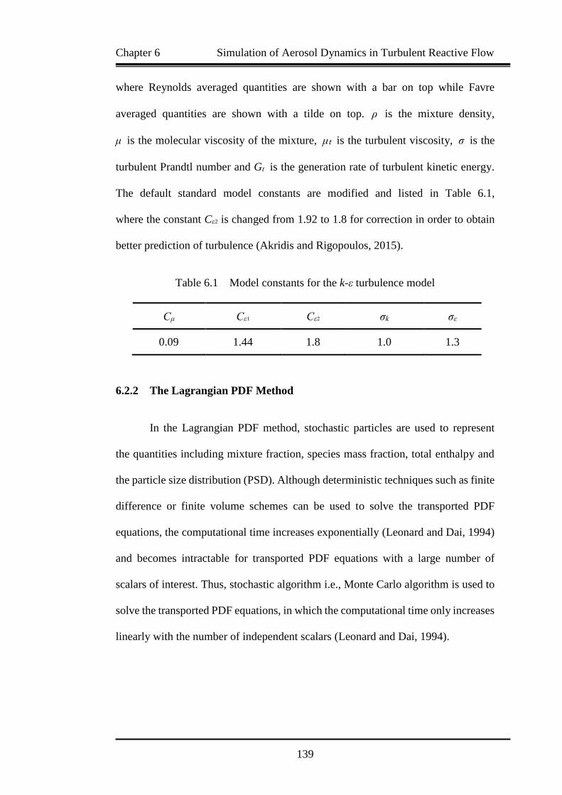
Chapter 6 Simulation of Aerosol Dynamics in Turbulent Reactive Flow
139
where Reynolds averaged quantities are shown with a bar on top while Favre
averaged quantities are shown with a tilde on top. ρ is the mixture density,
μ is the molecular viscosity of the mixture, μt is the turbulent viscosity, σ is the
turbulent Prandtl number and Gt is the generation rate of turbulent kinetic energy.
The default standard model constants are modified and listed in Table 6.1,
where the constant Cε2 is changed from 1.92 to 1.8 for correction in order to obtain
better prediction of turbulence (Akridis and Rigopoulos, 2015).
Table 6.1 Model constants for the k-ε turbulence model
Cμ Cε1 Cε2 σk σε
0.09 1.44 1.8 1.0 1.3
6.2.2 The Lagrangian PDF Method
In the Lagrangian PDF method, stochastic particles are used to represent
the quantities including mixture fraction, species mass fraction, total enthalpy and
the particle size distribution (PSD). Although deterministic techniques such as finite
difference or finite volume schemes can be used to solve the transported PDF
equations, the computational time increases exponentially (Leonard and Dai, 1994)
and becomes intractable for transported PDF equations with a large number of
scalars of interest. Thus, stochastic algorithm i.e., Monte Carlo algorithm is used to
solve the transported PDF equations, in which the computational time only increases
linearly with the number of independent scalars (Leonard and Dai, 1994).
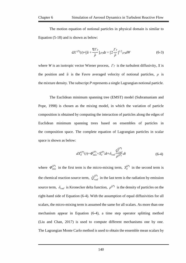
Chapter 6 Simulation of Aerosol Dynamics in Turbulent Reactive Flow
140
The motion equation of notional particles in physical domain is similar to
Equation (5-18) and is shown as below:
dX (P)(t)=[u +∇ΓT
ρ](P)dt + [2
ΓT
ρ]1/2
(P)dW
where W is an isotropic vector Wiener process, ΓT is the turbulent diffusivity, X is
the position and u is the Favre averaged velocity of notional particles, ρ is
the mixture density. The subscript P represents a single Lagrangian notional particle.
The Euclidean minimum spanning tree (EMST) model (Subramaniam and
Pope, 1998) is chosen as the mixing model, in which the variation of particle
composition is obtained by computing the interaction of particles along the edges of
Euclidean minimum spanning trees based on ensembles of particles in
the composition space. The complete equation of Lagrangian particles in scalar
space is shown as below:
dXa(P)(t)=Φmix
(P)+Sa
(P)dt+δrad
Qrad
(P)
ρ(P)dt
where Φmix(P)
in the first term is the micro-mixing term, Sa(P)
in the second term is
the chemical reaction source term, Qrad
(P) in the last term is the radiation by emission
source term, δrad is Kronecker delta function, ρ(P) is the density of particles on the
right-hand side of Equation (6-4). With the assumption of equal diffusivities for all
scalars, the micro-mixing term is assumed the same for all scalars. As more than one
mechanism appear in Equation (6-4), a time step operator splitting method
(Liu and Chan, 2017) is used to compute different mechanisms one by one.
The Lagrangian Monte Carlo method is used to obtain the ensemble mean scalars by
(6-3)
(6-4)

Chapter 6 Simulation of Aerosol Dynamics in Turbulent Reactive Flow
141
time averaging and then input the results to the CFD (RANS) code to close other
terms. The detailed procedures of one loop of Monte Carlo simulation can be found
in Chapter 5.
6.2.3 Particle Tracking Algorithm
The particle tracking algorithm of Subramaniam and Haworth (2000) is
adopted here. For a particle, j in cell, i, let the minimum time of particle, j to intersect
a face of cell, i be ti,j, and the time step be ∆t. If ti,j >∆t, the particle, j stays in cell,
i at the end of one time step. If ti,j <∆t, the particle, j is moved to the face intersection
point of cell, i at the end of one time step, and its cell pointer is updated and
time-step is decremented by ti,j. Repeat the tracking particles until the remaining time
of all the particles becomes zero. The total number of particles in a cell is maintained
within a prescribed range by cloning or destroying particles if a lower bound or upper
bound is reached. The time step, ∆ti in a cell is chosen to be the minimum time for
satisfying the turbulence time scale and CFL conditions in Chapter 5.
Moreover, the final time step ∆t is chosen to be the minimum amongst all the cells
in the computational domain as follows:
∆t=min{∆ti, i=1, 2,…,n} (6-5)
where n is the total number of cells in the computational domain.

Chapter 6 Simulation of Aerosol Dynamics in Turbulent Reactive Flow
142
6.2.4 Estimation of Mean Field
Estimates of mean quantities in PDF/Monte-Carlo simulation are obtained
by means of a particle-cloud-in-cell method and the Favre average of a quantity,
Q in a cell, c is shown as follows (Mehta, 2008):
Qc =∑ mpQpp∈c
∑ mpp∈c
where mp is the mass of particle p and Qp is the quantity carried by particle, p in
a cell, c. The summation is carried out over all the particles in cell, c.
6.2.5 Soot Model
An acetylene based soot model with only growth/oxidation and nucleation
processes (Akridis and Rigopoulos, 2015; Liu et al., 2003) is used in the present
study. According to the experimental results of the same jet flame (Brookes and
Moss, 1999), the soot volume concentration in the jet flame is only of magnitude
order 10-7, in which the coagulation events of soot particles hardly take place. Thus,
coagulation process is not included in the soot model here. An important assumption
is that the shape of soot particles is considered spherical. Nucleation and surface
growth rate are assumed the first-order dependent on acetylene concentration while
the oxidation rate is a function of molecular oxygen and hydroxyl concentrations,
which is as follows (Akridis and Rigopoulos, 2015):
Nucleation rate:
NU0 =2NAkn(T)[C2H2]
Cmin
(6-6)
(6-7)

Chapter 6 Simulation of Aerosol Dynamics in Turbulent Reactive Flow
143
Growth rate:
GSG =2kHW(T)[C2H2]As
ρs
Oxidation rates:
GO2 =120[
kαXO2χ1
1 + kzXO2+kbXO2(1 χ1)]As
ρs
GOH =
167XOH
√TAs
ρs
where k is reaction rate constant, a function of temperature. Cmin is the minimum
number of carbon atoms that is needed to produce an incipient soot particle,
which is assumed 700 here with an initial soot diameter of 2.4 nm (Liu et al., 2003).
NA is the Avogadro constant. The density of soot, ρs is assumed 1800 kg/m3.
As is the surface area of soot particles. X is the mole fraction of a species.
Other constants are set according to Hall et al. (1997) and Liu et al. (2003).
6.2.6 Radiation Model
An optically thin radiation model is chosen as the radiation model in
the present study where the gaseous phase and soot particles only emit radiation but
do not re-absorb any energy. The radiation coefficients are calculated according to
Akridis and Rigopoulos (2015). The radiation model with CH4, H2O, CO and CO2
taken into account is shown as follows:
Qrad = 4σ(T4 Tb4) ∑ piap,i
Nsp
i=1
+ 4σfv(T5 Tb
5)
(6-8)
(6-9b)
(6-9a)
(6-10)

Chapter 6 Simulation of Aerosol Dynamics in Turbulent Reactive Flow
144
where σ is the Stefan-Boltzmann constant, Tb is the background temperature of
the experiment and Nsp is the total number of species. pi is the partial pressure and
ap,i is the Planck mean absorption coefficient of species, i. fv is the volume fraction
of soot particles (Lindstedt and Louloudi, 2005).
6.3 Numerical Simulation Setup
The configuration of the combustor in the numerical simulation is shown in
Figure 6.1, which is a piloted non-premixed combustor in the experiment of Brookes
and Moss (1999). The combustor consists of a jet burner with internal diameter of
4.07 mm having a jet flame at 20.3 m/s. The Reynolds number of the jet at exit is
5000. An air co-flow is supplied at 0.5 m/s surrounding the central fuel tube.
A Pyrex tube with internal diameter of 156 mm and height of 600 mm is used to
confine the jet flame. The outlet of the burner is at 290 K and atmospheric pressure.
The detailed jet burner parameters of the studied combustor is shown in Table 6.2.

Chapter 6 Simulation of Aerosol Dynamics in Turbulent Reactive Flow
145
Figure 6.1 Jet burner configuration of the combustor (Brookes and Moss, 1999).
Table 6.2 Jet burner parameters and conditions for the studied combustor.
Absolute pressure 1 atm
Velocity of methane 20.3 m/s
Flow rate of methane 10.3 g/min
Inlet temperature of methane 290 K
Velocity of air 0.5 m/s
Flow rate of air 708 g/min
Inlet temperature of air 290 K
Reynolds number of jet flame exit, Rej 5000
Internal diameter of the burner 4.07 mm
Internal diameter of confined Pyrex tube 156 mm
Number of notional particles per cell 50

Chapter 6 Simulation of Aerosol Dynamics in Turbulent Reactive Flow
146
The computational domain is shown in Figure 6.2, which is
a two-dimensional (2D) axisymmetric jet domain. The non-uniform 2D grid is
generated with 160 points in the axial direction and 100 points in the radial direction.
There are totally 5542 cells and 5597 nodes in the grid. The number of notional
particles used for each cell is 50 to compute the scalar variables in the Lagrangian
PDF method. In addition, the scalar variables are time averaged with 3000 iterations
in order to reduce the statistical error. The mixture fraction is defined as the mass
fraction of species originating from the fuel stream amongst all the species,
which is used to characterize the instantaneous thermochemical state of
the non-premixed turbulent combustion in the present study.
Figure 6.2 The computational grid used in the numerical simulation of
an axisymmetric combustor.
z
r
Axis

Chapter 6 Simulation of Aerosol Dynamics in Turbulent Reactive Flow
147
The mixture fraction is defined as a normalized ratio by the following newly added
Equation (6-11), measuring the fuel/oxidizer ratio (Turns, 2011):
Z = sYF − YO+ (YO)0
sYF + (YO)0
where Z is the mixture fraction, YF is the molecular fraction of fuel in the mixture,
YO is the molecular fraction of oxygen in the mixture, (YO)0 is the initial molecular
fraction of fuel, s is the molecular ratio of fuel to oxidizer (i.e., air).
6.4 Results and Discussion
6.4.1 Axial and Radial Jet Temperature Variations of the Studied Combustor
In the present studied axisymmetric combustor, the jet temperature varies in
both radial and axial directions. It can be seen that axial distance is actually
the height above the inlet of the burner as shown in Figure 6.2. The simulation results
are compared with the classical experimental results available from Brookes and
Moss (1999). Figure 6.3 shows the axial jet temperature variation at the centerline
of the studied combustor for Rej = 5000. The numerical results agree well with
the experimental results. With increasing axial distance from zero (the inlet of the
burner) to 0.6 m, the sampling position in the jet flame moves from the inner layer
to the outer layer of methane flame, which corresponds to the increase of jet
temperature axially.
(6-11)

Chapter 6 Simulation of Aerosol Dynamics in Turbulent Reactive Flow
148
Figure 6.3 Axial jet temperature variation at the centerline of the studied
combustor for Rej=5000 (The experimental results are obtained from Brookes and
Moss (1999)).
Figure 6.4 shows the radial jet temperature variation at the axial distance of
250 mm for the studied combustor at Rej = 5000. Excellent agreement can be
observed between the jet temperature from numerical simulation and that from the
experiment of Brookes and Moss (1999). The radial distance of zero corresponds to
the centerline of the jet flame. With increasing radial distance from zero to 0.06 m,
the sampling position moves from the centerline of jet flame to the outer layer of
the methane flame and finally out of the flame region. Thus, the radial jet
temperature in Figure 6.4 increases first and then decreases when the sampling
position moves out of the flame region. It is obvious that the simulation results
obtained by the proposed coupled CFD-Monte Carlo method accurately capture
the radial jet temperature variation in the combustor.
0.0 0.1 0.2 0.3 0.4 0.5 0.60
500
1000
1500
2000
Tem
per
atu
re (
K)
Axial distance (m)
Numerical simulation results
Experimental results
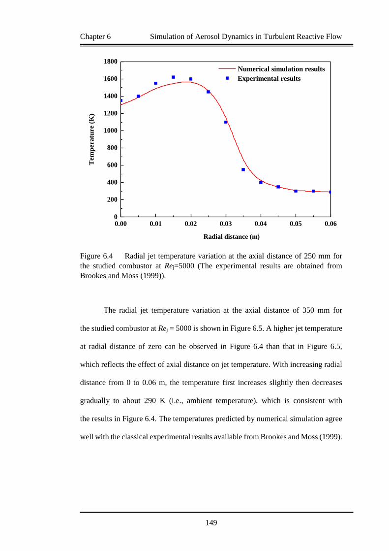
Chapter 6 Simulation of Aerosol Dynamics in Turbulent Reactive Flow
149
Figure 6.4 Radial jet temperature variation at the axial distance of 250 mm for
the studied combustor at Rej=5000 (The experimental results are obtained from
Brookes and Moss (1999)).
The radial jet temperature variation at the axial distance of 350 mm for
the studied combustor at Rej = 5000 is shown in Figure 6.5. A higher jet temperature
at radial distance of zero can be observed in Figure 6.4 than that in Figure 6.5,
which reflects the effect of axial distance on jet temperature. With increasing radial
distance from 0 to 0.06 m, the temperature first increases slightly then decreases
gradually to about 290 K (i.e., ambient temperature), which is consistent with
the results in Figure 6.4. The temperatures predicted by numerical simulation agree
well with the classical experimental results available from Brookes and Moss (1999).
0.00 0.01 0.02 0.03 0.04 0.05 0.060
200
400
600
800
1000
1200
1400
1600
1800
Tem
per
atu
re (
K)
Radial distance (m)
Numerical simulation results
Experimental results
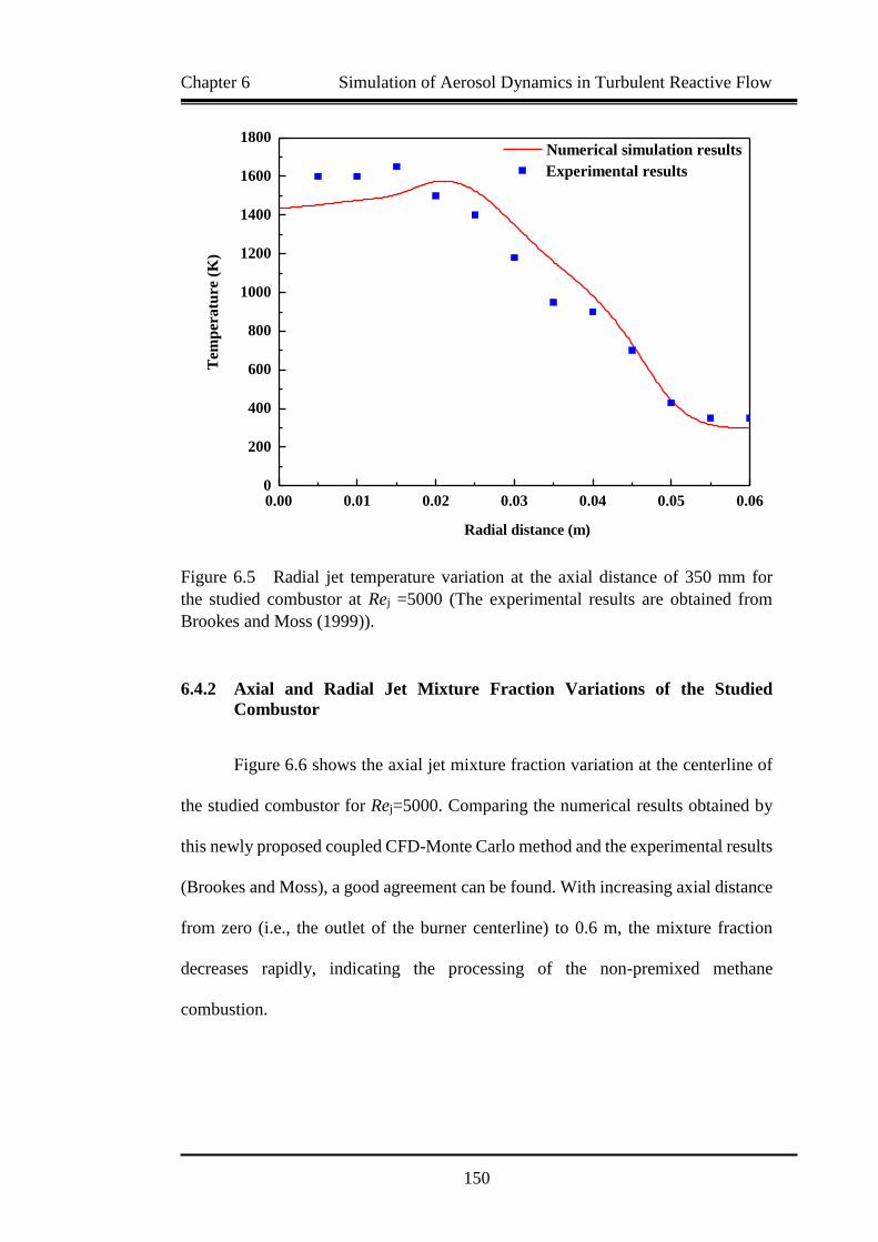
Chapter 6 Simulation of Aerosol Dynamics in Turbulent Reactive Flow
150
Figure 6.5 Radial jet temperature variation at the axial distance of 350 mm for
the studied combustor at Rej =5000 (The experimental results are obtained from
Brookes and Moss (1999)).
6.4.2 Axial and Radial Jet Mixture Fraction Variations of the Studied
Combustor
Figure 6.6 shows the axial jet mixture fraction variation at the centerline of
the studied combustor for Rej=5000. Comparing the numerical results obtained by
this newly proposed coupled CFD-Monte Carlo method and the experimental results
(Brookes and Moss), a good agreement can be found. With increasing axial distance
from zero (i.e., the outlet of the burner centerline) to 0.6 m, the mixture fraction
decreases rapidly, indicating the processing of the non-premixed methane
combustion.
0.00 0.01 0.02 0.03 0.04 0.05 0.060
200
400
600
800
1000
1200
1400
1600
1800
Tem
per
atu
re (
K)
Radial distance (m)
Numerical simulation results
Experimental results

Chapter 6 Simulation of Aerosol Dynamics in Turbulent Reactive Flow
151
Figure 6.6 Axial jet mixture fraction variation at the centerline of the studied
combustor for Rej =5000 (The experimental results are obtained from Brookes and
Moss (1999)).
The radial jet mixture fraction variation at the axial distance of 250 mm for
the studied combustor at Rej =5000 is shown in Figure 6.7. The numerical results
obtained agree well with the experimental results despite slight over prediction of
mixture fraction. However, the discrepancy at 0.005 m in the radial distance may be
caused by the instability and stagnation region of jet flame. With increasing radial
distance from 0 to 0.04 mm, the mixture fraction in Figure 6.8 decreases gradually
to almost zero at 0.04 mm in the radial direction.
0.0 0.1 0.2 0.3 0.4 0.5 0.60.0
0.2
0.4
0.6
0.8
1.0
Mix
ture
fra
ctio
n
Axial distance (m)
Numerical simulation results
Experimental results

Chapter 6 Simulation of Aerosol Dynamics in Turbulent Reactive Flow
152
Figure 6.7 Radial jet mixture fraction variation at the axial distance of 250 mm for
the studied combustor at Rej =5000 (The experimental results are obtained from
Brookes and Moss (1999)).
Figure 6.8 shows the radial jet mixture fraction variation at the axial distance
of 350 mm for the studied combustor at Rej =5000. Good agreement can be obtained
between the numerical results and the experimental results except for the mixture
fraction at the radial distance of 0 mm (i.e., centerline of jet flame) which may be
caused due to the instability and stagnation region of jet flame. Comparing the
mixture fraction in Figures 6.7 and 6.8, it can be found that the mixture fraction at
250 mm in the axial direction is higher than that at 350 mm in the axial direction if
radial distance is less than 0.03 m. With increasing radial distance from 0 to
0.04 mm, the mixture fraction in Figure 6.8 decreases gradually to a stable value at
0.04 mm in the radial direction. The higher mixture fraction at 0.04 m in Figure 6.8
0.00 0.01 0.02 0.03 0.040.00
0.05
0.10
0.15
0.20
0.25
Mix
ture
fracti
on
Radial distance (m)
Numerical simulation results
Experimental results
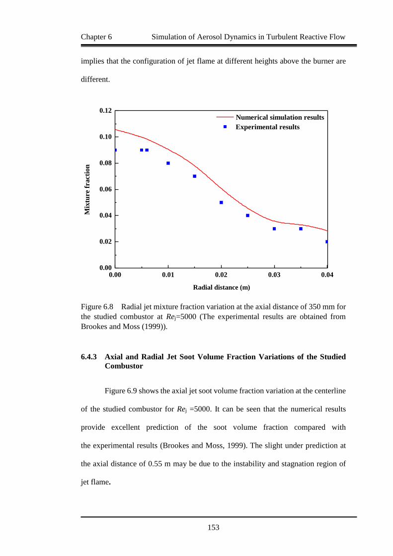
Chapter 6 Simulation of Aerosol Dynamics in Turbulent Reactive Flow
153
implies that the configuration of jet flame at different heights above the burner are
different.
Figure 6.8 Radial jet mixture fraction variation at the axial distance of 350 mm for
the studied combustor at Rej=5000 (The experimental results are obtained from
Brookes and Moss (1999)).
6.4.3 Axial and Radial Jet Soot Volume Fraction Variations of the Studied
Combustor
Figure 6.9 shows the axial jet soot volume fraction variation at the centerline
of the studied combustor for Rej =5000. It can be seen that the numerical results
provide excellent prediction of the soot volume fraction compared with
the experimental results (Brookes and Moss, 1999). The slight under prediction at
the axial distance of 0.55 m may be due to the instability and stagnation region of
jet flame.
0.00 0.01 0.02 0.03 0.040.00
0.02
0.04
0.06
0.08
0.10
0.12
Mix
ture
fra
ctio
n
Radial distance (m)
Numerical simulation results
Experimental results

Chapter 6 Simulation of Aerosol Dynamics in Turbulent Reactive Flow
154
Figure 6.9 Axial jet soot volume fraction variation at the centerline of the studied
combustor for Rej = 5000 (The experimental results are obtained from Brookes and
Moss (1999)).
Comparing Figure 6.9 with Figure 6.3, it can be seen that as jet temperature
increases with the axial distance, the soot volume fraction increases accordingly,
implying that high jet temperature is conducive to the formation of soot particles.
This can be explained from the Equations (6.7) to (6.9). As jet temperature increases,
the aerosol dynamic processes including nucleation, growth and oxidation are all
accelerated, resulting in the increase of soot volume fraction in the axial direction.
Figure 6.10 shows the radial jet soot volume fraction variation at the axial
distance of 350 mm for the studied combustor at Rej = 5000. An excellent agreement
between the numerical results and experimental results can be obtained in
Figure 6.10. With increasing radial distance from 0 to 0.05 m, an obvious gradient
of soot volume fraction can be observed. Comparing Figure 6.10 with Figure 6.5,
0.0 0.1 0.2 0.3 0.4 0.5 0.60.0
0.2
0.4
0.6
0.8
1.0
1.2
1.4
1.6
1.8
2.0
Soot
volu
me
fract
ion
()
Axial distance (m)
Numerical simulation results
Experimental results

Chapter 6 Simulation of Aerosol Dynamics in Turbulent Reactive Flow
155
it can be found that the higher soot volume fraction corresponds to higher jet
temperature. As jet temperature decreases in the radial direction, the soot volume
fraction decreases accordingly. The numerical simulation with the newly proposed
coupled CFD-Monte Carlo method demonstrates high capability in capturing
the variation of soot volume fraction in the non-premixed turbulent jet flame of
methane.
Figure 6.10 Radial jet soot volume fraction variation at the axial distance of
350 mm for the studied combustor at Rej=5000 (The experimental results are
obtained from Brookes and Moss (1999)).
A similar radial jet soot volume fraction variation at the axial distance of
425 mm above the burner for the studied combustor at Rej=5000 in Figure 6.11. With
the increase of radial distance, the soot volume fraction decreases obviously. An
excellent agreement can be obtained between the numerical results and the
experimental results of Brooke and Moss (1999). The variation of jet soot volume
0.00 0.01 0.02 0.03 0.04 0.050.0
0.2
0.4
0.6
0.8
1.0
1.2
1.4
Soot
volu
me
fract
ion
()
Radial distance (m)
Numerical simulation results
Experimental results
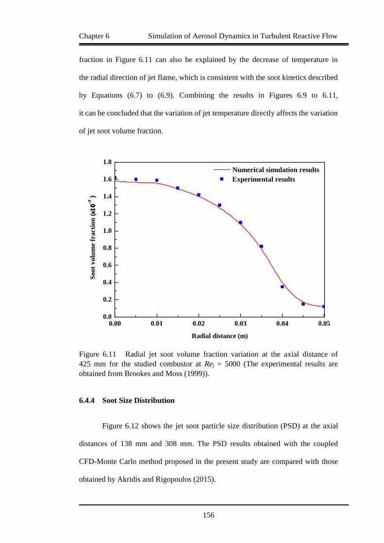
Chapter 6 Simulation of Aerosol Dynamics in Turbulent Reactive Flow
156
fraction in Figure 6.11 can also be explained by the decrease of temperature in
the radial direction of jet flame, which is consistent with the soot kinetics described
by Equations (6.7) to (6.9). Combining the results in Figures 6.9 to 6.11,
it can be concluded that the variation of jet temperature directly affects the variation
of jet soot volume fraction.
Figure 6.11 Radial jet soot volume fraction variation at the axial distance of
425 mm for the studied combustor at Rej = 5000 (The experimental results are
obtained from Brookes and Moss (1999)).
6.4.4 Soot Size Distribution
Figure 6.12 shows the jet soot particle size distribution (PSD) at the axial
distances of 138 mm and 308 mm. The PSD results obtained with the coupled
CFD-Monte Carlo method proposed in the present study are compared with those
obtained by Akridis and Rigopoulos (2015).
0.00 0.01 0.02 0.03 0.04 0.050.0
0.2
0.4
0.6
0.8
1.0
1.2
1.4
1.6
1.8
Soot
volu
me
fract
ion
()
Radial distance (m)
Numerical simulation results
Experimental results
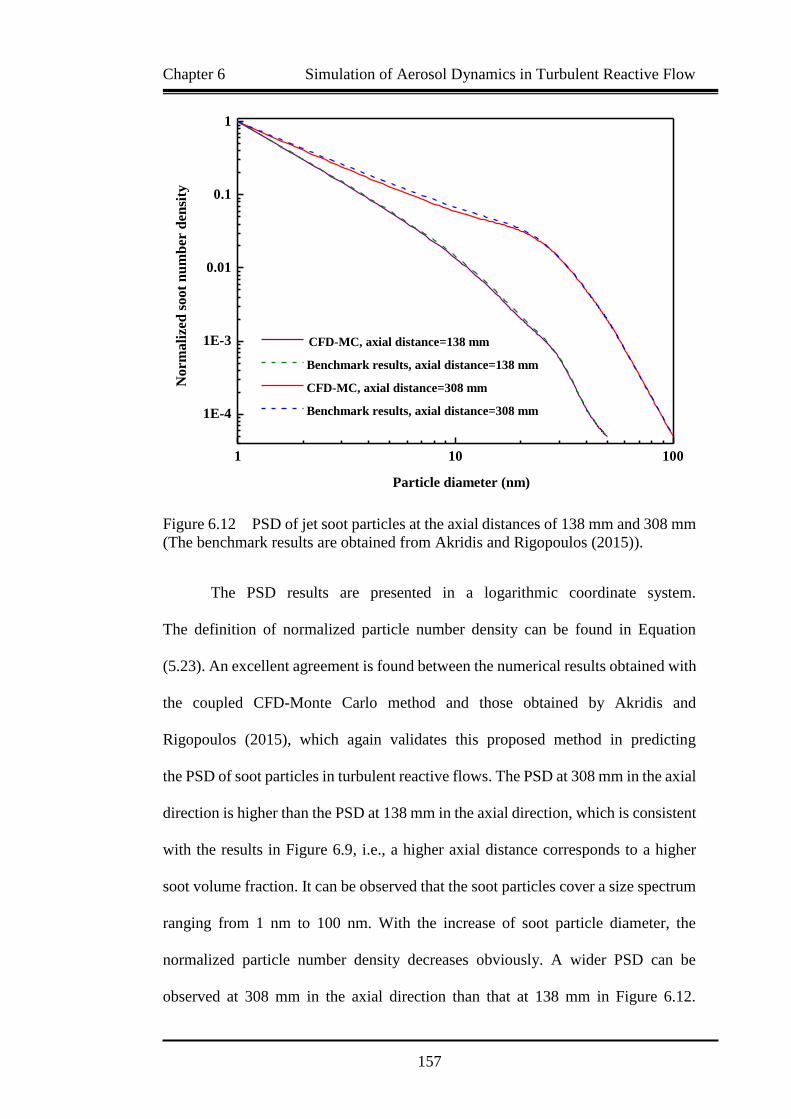
Chapter 6 Simulation of Aerosol Dynamics in Turbulent Reactive Flow
157
Figure 6.12 PSD of jet soot particles at the axial distances of 138 mm and 308 mm
(The benchmark results are obtained from Akridis and Rigopoulos (2015)).
The PSD results are presented in a logarithmic coordinate system.
The definition of normalized particle number density can be found in Equation
(5.23). An excellent agreement is found between the numerical results obtained with
the coupled CFD-Monte Carlo method and those obtained by Akridis and
Rigopoulos (2015), which again validates this proposed method in predicting
the PSD of soot particles in turbulent reactive flows. The PSD at 308 mm in the axial
direction is higher than the PSD at 138 mm in the axial direction, which is consistent
with the results in Figure 6.9, i.e., a higher axial distance corresponds to a higher
soot volume fraction. It can be observed that the soot particles cover a size spectrum
ranging from 1 nm to 100 nm. With the increase of soot particle diameter, the
normalized particle number density decreases obviously. A wider PSD can be
observed at 308 mm in the axial direction than that at 138 mm in Figure 6.12.
1 10 100
1E-4
1E-3
0.01
0.1
1
Norm
ali
zed
soot
nu
mb
er d
en
sity
Particle diameter (nm)
CFD-MC, axial distance=138 mm
Benchmark results, axial distance=138 mm
CFD-MC, axial distance=308 mm
Benchmark results, axial distance=308 mm
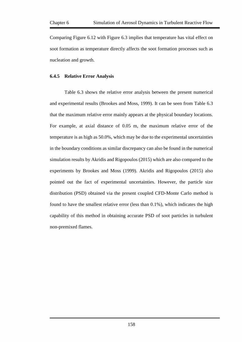
Chapter 6 Simulation of Aerosol Dynamics in Turbulent Reactive Flow
158
Comparing Figure 6.12 with Figure 6.3 implies that temperature has vital effect on
soot formation as temperature directly affects the soot formation processes such as
nucleation and growth.
6.4.5 Relative Error Analysis
Table 6.3 shows the relative error analysis between the present numerical
and experimental results (Brookes and Moss, 1999). It can be seen from Table 6.3
that the maximum relative error mainly appears at the physical boundary locations.
For example, at axial distance of 0.05 m, the maximum relative error of the
temperature is as high as 50.0%, which may be due to the experimental uncertainties
in the boundary conditions as similar discrepancy can also be found in the numerical
simulation results by Akridis and Rigopoulos (2015) which are also compared to the
experiments by Brookes and Moss (1999). Akridis and Rigopoulos (2015) also
pointed out the fact of experimental uncertainties. However, the particle size
distribution (PSD) obtained via the present coupled CFD-Monte Carlo method is
found to have the smallest relative error (less than 0.1%), which indicates the high
capability of this method in obtaining accurate PSD of soot particles in turbulent
non-premixed flames.

Chapter 6 Simulation of Aerosol Dynamics in Turbulent Reactive Flow
159
Table 6.3 Relative error analysis between the present numerical and experimental
results (Brookes and Moss, 1999).
Temperature Mixture fraction
Soot volume
fraction PSD
Position
(m)
Error
(%)
Position
(m)
Error
(%)
Position
(m)
Error
(%)
Value
(%)
Axial
direction 0.05 50.0 0.05 16.7 0.55 11.1 N/A
Radial
direction 0.35 14.0 0.05 15.0 0.05 4.3 <0.1
Note: The “relative error” is defined by Equation (4.18). “Position” is used to
represent the axial or radial distance of the sampling point at which the
corresponding relative error appears. Particle size distribution (PSD) is taken in the
radial direction in the experiments (Brookes and Moss, 1999), but no PSD results
are given in the axial direction. N/A: not applicable.
6.5 Summary
The newly proposed and validated CFD-Monte Carlo method in Chapter 5
is used together with the soot and radiation models to investigate aerosol dynamics
i.e., soot dynamics in non-premixed turbulent reactive flows. The variation of jet
temperature, and mixture fraction and soot volume fractions in both axial and radial
direction are obtained and compared with experimental results of Brookes and Moss
(1999). Excellent agreement is obtained between the numerical results and
the experimental results, which validates the reliability and capability of this
proposed method. Moreover, the PSDs of jet soot particles at different axial
distances predicted by this newly modified and developed CFD-Monte Carlo
method agree very well with the results of Akridis and Rigopoulos (2015).
The numerical results demonstrate that temperature is of great significance to soot
dynamics and high temperature is conducive to the formation of soot particles in the
present studied low sooty flame. However, considering the low soot volume
Chapter 6 Simulation of Aerosol Dynamics in Turbulent Reactive Flow
160
concentration in the studied flame (< 0.2 ppm), it should not be interpreted to be of
any generality in other turbulent sooty flames. Relative error analysis of the
numerical simulation results shows that the highest discrepancy with the
experimental results (Brookes and Moss, 1999) appears at boundary locations in the
jet flame, which may be due to the uncertainties of the experimental boundary
conditions. However, the present modified CFD-Monte Carlo method still
demonstrates high capability of obtaining PSD with high accuracy.

Chapter 7 Conclusions and Recommendations for Future Work
161
Chapter 7 Conclusions and Recommendations for Future Work
7.1 Review of the Present Research
This thesis is mainly focused on the numerical simulation of multi-scale and
multi-dimensional turbulent reactive flows with the newly proposed and developed
computational fluid dynamics (CFD) based Monte Carlo method. The research work
in this thesis can be divided into three major parts:
In the first part of the current research, a newly proposed and developed
stochastically weighted operator splitting Monte Carlo (SWOSMC) method is used
for the simulation of complex aerosol dynamics. Stochastically weighted particle
method is coupled with operator splitting method to formulate the SWOSMC
method for the numerical simulation of particle-fluid systems undergoing
the complex simultaneous aerosol dynamic processes. The studied cases cover all
the typical aerosol dynamic processes including coagulation, nucleation, growth and
condensation. This proposed SWOSMC method is first validated by comparing its
numerical simulation results of constant rate coagulation and linear rate
condensation with the corresponding analytical solutions. Coagulation and
nucleation cases are further studied and the results show excellent agreement with
the sectional method. This newly proposed SWOSMC method has also
demonstrated its high numerical simulation capability when used to deal with
simultaneous aerosol dynamic processes including coagulation, nucleation and
condensation.

Chapter 7 Conclusions and Recommendations for Future Work
162
The second part of the current research is the development of
a CFD-population balance modelling (PBM) method for simulating aerosol
dynamics in turbulent flows. The validated SWOSMC method in Chapter 4 is further
modified and coupled with CFD method based on the transported probability density
function (PDF) approach. The formulated CFD-Monte Carlo method allows
investigating the interaction between turbulence and aerosol dynamics, and
incorporating individual aerosol dynamic kernels as well as obtaining full particle
size distribution (PSD). Several typical cases of aerosol dynamic processes including
turbulent coagulation, nucleation and growth processes are studied and compared to
the sectional method with excellent agreement. Coagulation in both laminar and
turbulent flows is simulated and compared to demonstrate the effect of turbulence
on aerosol dynamics. The effect of different jet Reynolds (Rej) numbers on aerosol
dynamics in turbulent flows is fully investigated for each of the studied cases.
The third part of the current research is the simulation of aerosol dynamics
in turbulent reactive flows by using the newly proposed and developed CFD-PBM
method together with GRI 1.2 combustion chemistry and soot kinetics models.
Soot formation in turbulent non-premixed flames of methane as well as its
interaction with radiation is studied. The particle representations of mixture fraction,
species, enthalpy and distribution of soot number density are solved using
the Lagrangian particle method. Both turbulence-radiation and turbulence-chemistry
interactions are considered.
Chapter 7 Conclusions and Recommendations for Future Work
163
7.2 Main Conclusions of the Thesis
7.2.1 Conclusions of the Zero-Dimensional Monte Carlo Simulation of
Aerosol Dynamics
The simulation results of this newly proposed and developed stochastically
weighted operator splitting Monte Carlo (SWOSMC) method are fully validated
with corresponding analytical solutions (Ramabhadran et al., 1976; Maisels et al.,
2004) and the sectional method (Prakash et al., 2003) for various aerosol dynamic
processes (i.e., coagulation, condensation and nucleation) in different flow regimes.
Excellent results are obtained from this new SWOSMC method. For just an average
number of numerical particles 2000 used, the maximum relative error is less than
1%.
With the increase of the complexity from the studied Case 1 to Case 4,
an increasing computational time is obviously required for using a fixed number of
numerical particles. However, for a certain case, the computational error is inversely
proportional to the square root of the total number of the numerical particles (Oran
et al., 1998). It also suggests that further optimization of this newly proposed
SWOSMC method is needed in order to improve the computational efficiency and
accuracy for the complex particle-fluid systems. Compared with the sectional
method (Prakash et al., 2003), this newly proposed SWOSMC method takes a much
shorter computational time even with the largest number of numerical particles in
the studied Case 3.
There always exists conflicts and tradeoffs between computational cost (i.e.,
computational time, computer memory, etc.) and accuracy for Monte Carlo based

Chapter 7 Conclusions and Recommendations for Future Work
164
methods for the numerical simulation of complex aerosol dynamics.
However, this validated SWOSMC method has clearly demonstrated a promising
high capacity to obtain higher computational accuracy and efficiency with a much
shorter computational time than the sectional method for the same typical studied
case.
7.2.2 Conclusions of the CFD-PBM Simulation of Aerosol Dynamics in
Turbulent Flows
Typical simultaneous aerosol dynamic processes including coagulation,
nucleation and growth are widely encountered in turbulent flows.
They are investigated with this newly proposed and developed Lagrangian particle
method based CFD-Monte Carlo method.
The effect of different Rej numbers on the interaction between turbulence
and aerosol dynamics is fully investigated. The results reveal the significant impact
of Rej on both single aerosol process (e.g. pure coagulation) and the competitive and
simultaneous aerosol dynamics processes in turbulent flows. The newly proposed
CFD-Monte Carlo/PDF method renders an efficient method to deal with
the interaction between turbulence and aerosol dynamics by overcoming the closure
problems.
The full particle size ditribution (PSD) of aerosol particles is readily obtained.
The enhancing effect of turbulence on coagulation is demonstrated by comparison
of laminar coagulation and turbulent coagulation. Further investigation of the effect
of turbulence on the PSDs of simultaneous aerosol dynamics reveals the competition
between aerosol dynamic processes, which also has significant impact on the final

Chapter 7 Conclusions and Recommendations for Future Work
165
PSD of particles. For simultaneous complex aerosol dynamics in turbulent flows,
turbulence has an effect of broadening the PSD. The coupled CFD-Monte Carlo/PDF
method also shows excellent numerical stability according to typical grid cell
independence analysis and typical analysis of the number of simulation particles per
grid cell.
7.2.3 Conclusions of Simulation of Aerosol Dynamics in Turbulent Reactive
Flows
The variation of jet temperature, and mixture and soot volume fractions in
both axial and radial directions of a turbulent non-premixed jet flame of methane are
obtained and compared with the classical experimental results available from
Brookes and Moss (1999). Excellent agreement is found between the numerical and
the experimental results, which validates the high reliability of this newly proposed
and developed CFD-PBM method coupled with combustion chemistry and soot
kinetics models.
Moreover, the PSDs of jet soot particles at different axial distances predicted
by the newly proposed and developed CFD-Monte Carlo method agree very well
with the results obtained from Akridis and Rigopoulos (2015). The numerical results
demonstrate clearly that temperature is of great significance to soot dynamics and
high temperature is conducive to the formation of soot particles for this special low
sooty flame. Relative error analysis of the numerical results shows that the highest
discrepancy with the experimental results (Brookes and Moss, 1999) appears at
boundary locations in the jet flame, which may be due to the uncertainties of the
experimental boundary conditions. However, the present modified CFD-Monte
Carlo method still demonstrates high capability of obtaining PSD with high accuracy.
Chapter 7 Conclusions and Recommendations for Future Work
166
7.3 Recommendations for Future Work
The thesis presents the numerical simulation of typical and complex aerosol
dynamic processes ranging from zero-dimensional complex aerosol dynamics to
multi-dimensional aerosol dynamics in reactive flows with consideration of
the effect of turbulence. Based on the coupled stochastic weighted particle and
operator splitting methods, the aim of the thesis is to propose a robust and highly
efficient CFD-Monte Carlo method for solving complex aerosol dynamics in multi-
scale systems. Multi-dimensional aerosol dynamics and transport as well as
interaction with turbulence and reactive flows are fully investigated in the thesis with
this newly proposed and developed SWOSMC and CFD-Monte Carlo methods.
However, further research work is still recommended to overcome the limitations of
these proposed numerical methods and optimizations are also needed to make
the methods more robust and powerful.
7.3.1 Limitations of the Current Research
The limitations of this newly proposed and developed SWOSMC and CFD-
Monte Caro methods are as follows:
1. The two-dimensional axisymmetric grid cells are used for the numerical
simulation of aerosol dynamics in turbulent reactive flow.
However, for practical applications, aerosol reactors with arbitrary
configuration are widely encountered. Thus, a three-dimensional simulation
can be performed to further validate this newly proposed and developed
method, subject to the relevant and appropriate experimental datasets

Chapter 7 Conclusions and Recommendations for Future Work
167
available and accessible in literature for the study on the complexity of
aerosol processes and phenomena.
2. Parallel computing is not implemented in the present study. Considering the
stochastic motion of large number of Monte Carlo numerical particles, a
parallel computing approach may further improve the computational
efficiency and accuracy of the numerical simulation with this newly
proposed and developed method; and
3. Due to the fact that very few analytical solutions and experimental data are
available for complex aerosol dynamics in literature especially for aerosol
dynamic processes in turbulent reactive flows, the validation of this newly
proposed and developed methods is therefore limited to mainly comparing
with other numerical methods. Only for very limited cases, validation can be
performed by comparing with the analytical/experimental results available
in literature.
7.3.2 Recommendations for Future Work
Considering the above-mentioned limitations on the present study,
recommendations are made as follows:
1. Three-dimensionalization. The programs of this newly proposed methods
can be modified and optimized so that they can be fully applied to
three-dimensional simulations of complex aerosol dynamics in aerosol
reactors or other fluid-particle systems with arbitrary configurations for
validation, but subject to the relevant availability and accessibility of the
Chapter 7 Conclusions and Recommendations for Future Work
168
three-dimensional experimental datasets in literature. Moreover, with
appropriate modifications to this proposed and developed CFD-Monte Carlo
method, the large eddy simulation (LES) model can be applied to provide
better insight into the interaction between aerosol dynamics and turbulence;
2. Parallelization. In order to reduce computational cost (i.e., computational
time, computer memory, etc.) and increase computational efficiency,
parallelization of the source codes of these proposed and developed
numerical methods is required which is consistent with
the three-dimensionalization of these methods. It is because
three-dimensional simulation with more complicated turbulence models
requires higher computational cost.
3. Experimental investigations. More results from the related experiments are
needed in order to provide more reliable experimental data for the numerical
validation. Individually designed experiments are necessary to obtain
first-hand reliable results and validate these proposed and developed
numerical methods.
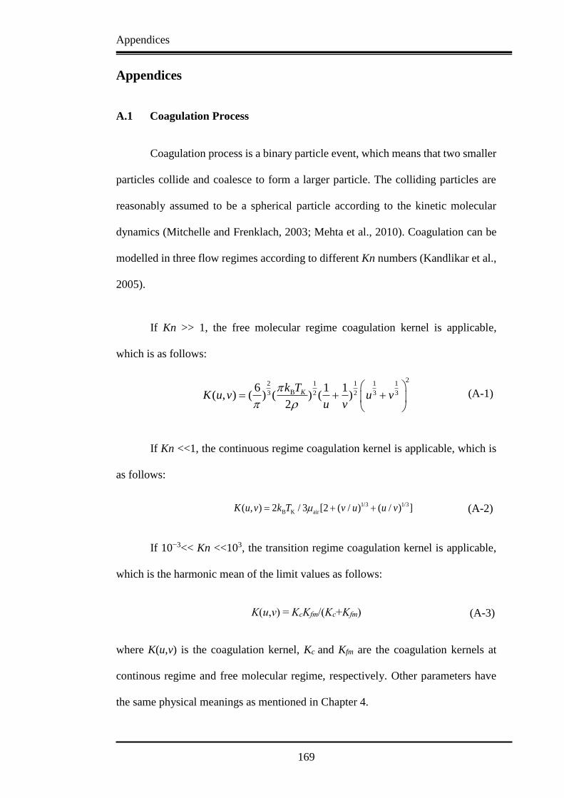
Appendices
169
Appendices
A.1 Coagulation Process
Coagulation process is a binary particle event, which means that two smaller
particles collide and coalesce to form a larger particle. The colliding particles are
reasonably assumed to be a spherical particle according to the kinetic molecular
dynamics (Mitchelle and Frenklach, 2003; Mehta et al., 2010). Coagulation can be
modelled in three flow regimes according to different Kn numbers (Kandlikar et al.,
2005).
If Kn >> 1, the free molecular regime coagulation kernel is applicable,
which is as follows:
22 1 11 1
B3 3 32 26 1 1
( , ) ( ) ( ) ( )2
Kk TK u v u v
u v
If Kn <<1, the continuous regime coagulation kernel is applicable, which is
as follows:
1/3 1/3
B K air( , ) 2 / 3 [2 ( / ) ( / ) ]K u v k T v u u v
If 10−3<< Kn <<103, the transition regime coagulation kernel is applicable,
which is the harmonic mean of the limit values as follows:
K(u,v) = KcKfm/(Kc+Kfm)
where K(u,v) is the coagulation kernel, Kc and Kfm are the coagulation kernels at
continous regime and free molecular regime, respectively. Other parameters have
the same physical meanings as mentioned in Chapter 4.
(A-1)
(A-2)
(A-3)

Appendices
170
A.2 Nucleation Process
Nucleation a single particle event, which generates the smallest size particles
in soot formation. The general equation of nucleation can be written as follows
(Kazakov and Frenklach, 1998):
dN0
dt= R0 G0 kss0Ng0/∆m
where Ng0 is the number density of newly generated smallest size particles,
R0 is the chemical rate that creates the smallest size particles, G0 is the reduction rate
of the smallest size particles by coagulation. The last term on the right-hand side of
Equation (A-4) is the reduction rate of the smallest size particles by surface reaction
where ks is the reaction rate per unit area, s0 is the surface area of the smallest size
particles and ∆m is the change during a single reaction event.
A.3 Surface Reactions in Soot Formation
The soot surface reactions using the Hydrogen-abstraction-Carbon-addition
mechanism is shown as follows (Frenklach and Wang, 1994; Wang et al., 1996):
Cs + H ⇌ Cs* + H2
Cs + OH ⇋ Cs* + H2O
Cs* + H → Cs
Cs + C2H2 → Cs + H
Cs + C2H2 → Cs* + H
Cs* + O2 → 2CO + products
Cs*+OH → CO + products
(A-4)
(A-5)
(A-6)
(A-7)
(A-8)
(A-9)
(A-10)
(A-11)
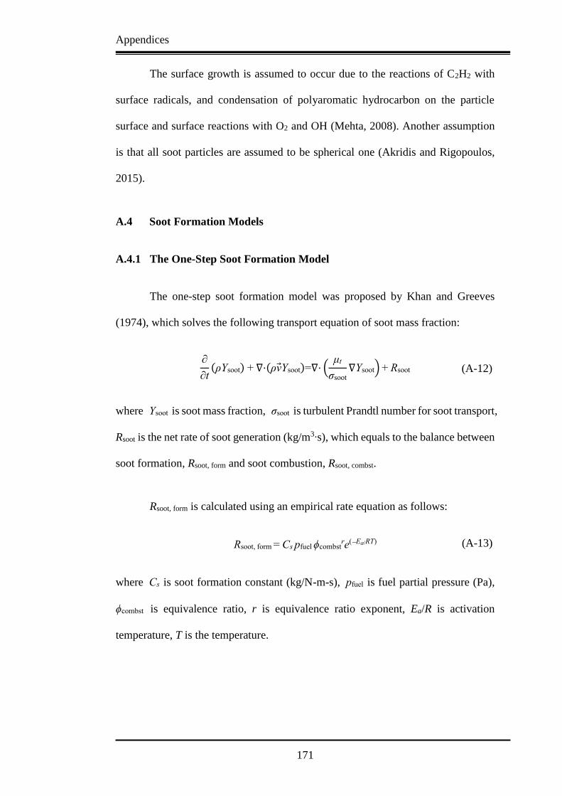
Appendices
171
The surface growth is assumed to occur due to the reactions of C2H2 with
surface radicals, and condensation of polyaromatic hydrocarbon on the particle
surface and surface reactions with O2 and OH (Mehta, 2008). Another assumption
is that all soot particles are assumed to be spherical one (Akridis and Rigopoulos,
2015).
A.4 Soot Formation Models
A.4.1 The One-Step Soot Formation Model
The one-step soot formation model was proposed by Khan and Greeves
(1974), which solves the following transport equation of soot mass fraction:
∂
∂t(ρYsoot) + ∇⋅(ρv Ysoot)=∇⋅ (
μt
σsoot∇Ysoot) + Rsoot
where Ysoot is soot mass fraction, σsoot is turbulent Prandtl number for soot transport,
Rsoot is the net rate of soot generation (kg/m3∙s), which equals to the balance between
soot formation, Rsoot, form and soot combustion, Rsoot, combst.
Rsoot, form is calculated using an empirical rate equation as follows:
Rsoot, form = Cs pfuel ϕcombstre(Ea/RT)
where Cs is soot formation constant (kg/N-m-s), pfuel is fuel partial pressure (Pa),
ϕcombst is equivalence ratio, r is equivalence ratio exponent, Ea/R is activation
temperature, T is the temperature.
(A-12)
(A-13)
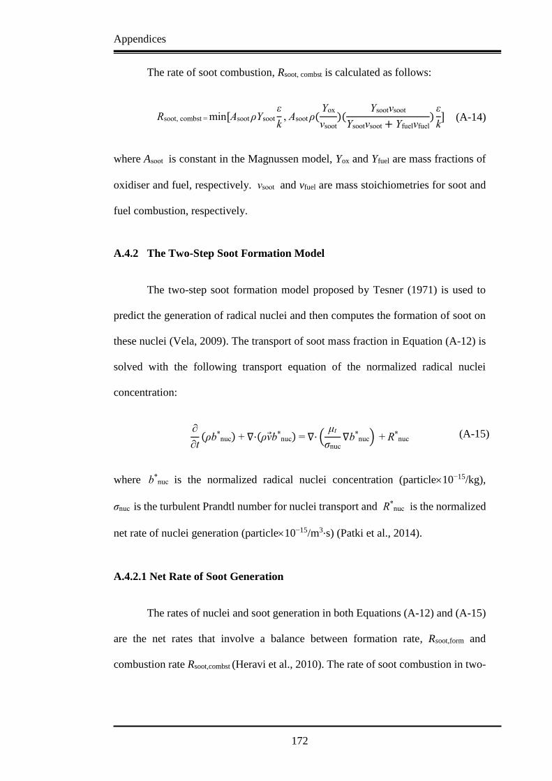
Appendices
172
The rate of soot combustion, Rsoot, combst is calculated as follows:
Rsoot, combst = min [Asoot ρYsoot
ε
k, Asoot ρ(
Yox
vsoot)(
Ysootvsoot
Ysootvsoot + Yfuelvfuel)
ε
k]
where Asoot is constant in the Magnussen model, Yox and Yfuel are mass fractions of
oxidiser and fuel, respectively. vsoot and vfuel are mass stoichiometries for soot and
fuel combustion, respectively.
A.4.2 The Two-Step Soot Formation Model
The two-step soot formation model proposed by Tesner (1971) is used to
predict the generation of radical nuclei and then computes the formation of soot on
these nuclei (Vela, 2009). The transport of soot mass fraction in Equation (A-12) is
solved with the following transport equation of the normalized radical nuclei
concentration:
∂
∂t(ρb*
nuc) + ∇⋅(ρv b*nuc) = ∇⋅ (
μt
σnuc∇b*
nuc) + R*nuc
where b*nuc is the normalized radical nuclei concentration (particle10−15/kg),
σnuc is the turbulent Prandtl number for nuclei transport and R*nuc is the normalized
net rate of nuclei generation (particle10−15/m3⋅s) (Patki et al., 2014).
A.4.2.1 Net Rate of Soot Generation
The rates of nuclei and soot generation in both Equations (A-12) and (A-15)
are the net rates that involve a balance between formation rate, Rsoot,form and
combustion rate Rsoot,combst (Heravi et al., 2010). The rate of soot combustion in two-
(A-14)
(A-15)
Appendices
173
step model is calculated similarly to the one-step model (Equation (A-14)), while
the rate of soot formation is calculated as follows:
Rsoot, form = mp(αβNsoot)cnuc
where mp is the average mass of soot particle (kg), Nsoot is the soot particle
concentration, cnuc is the concentration radical nuclei (/m3), α and β are
the empirical constants.
A.4.2.2 Net Rate of Nuclei Generation
The net rate of nuclei generation is given by the balance of nuclei formation
rate, R*nuc,form (particles10−15/m3-s) and combustion rate, R*
nuc, combst
(particles10−15/m3-s) (Peglow et al., 2006):
R*nuc = R*
nuc,form R*nuc, combst
In two-step model, the rates of nuclei formation and combustion are
calculated as follows (Patki et al., 2014):
R*nuc, form = a0*cfuele
(-Ea/RT) + (f g)soot c*nuc g0 c
*nucNsoot
where c*nuc is the normalized nuclei concentration, a0* is pre-exponential rate
constant, cfuel is fuel concentration (kg/m3), (f g)soot is the linear
branching-termination coefficient (s−1), g0 is the linear termination term of soot
particles (m3/particle-s) (Patki et al., 2014).
The rate of the combustion of nuclei is regarded as the linear function of
the rate of soot combusiton Rsoot,combst in Equation (A-14):
(A-16)
(A-17)
(A-18)

Appendices
174
R*nuc, combst = Rsoot,combst
b*nuc
Ysoot
where b*nuc is the normalized radical nuclei concentration (particle10-15/kg) and
Ysoot is soot mass fraction.
A.4.3 The Moss-Brookes Model
Both the transport equaitons of normalized radical nuclei concentration,
b*nuc and soot mass fraction, Ysoot are solved in the Moss-Brookes soot formation
model (Brookes and Moss, 1999), which are shown as follows:
∂
∂t(ρYsoot) + ∇⋅(ρv Ysoot)=∇⋅ (
μt
σsoot∇Ysoot) +
dM
dt
∂
∂t(ρb*
nuc) + ∇⋅(ρv b*nuc) = ∇⋅ (
μt
σnuc∇b*
nuc)+1
Nnorm
dN
dt
where M is soot mass concentration, N is soot particle number density and
Nnorm = 1015 particles.
The instantaneous generation rate of soot particles due to nucleation and
free molecular coagulation, is shown as follows:
dN
dt = CαNA( XprecP RT⁄ )l exp (
Tα
T) Cβ( 24RT ρsoot NA⁄ )1/2dp
1/2N2
where Cα, Cβ and l are dimensionless constants of the model, NA is Avogadro
number, Xprec is the mole concentration of soot precursor, ρsoot is soot mass density,
dp is the mean diameter of soot particles and Tα is the activation temperature for
nucleation reaction.
(A-22)
(A-19)
(A-21)
(A-20)
Appendices
175
The source term of soot formation process is shown as follows:
dM
dt = MP Cα ( XprecP RT⁄ )l exp (
Tα
T)
+ Cγ ( XsgsP RT⁄ )m exp (Tγ
T) [(πN)1/3(6M ρsoot⁄ )2/3]n
Coxid Cω ηcoll (XOHP
RT)√T (πN)1/3(6M ρsoot⁄ )2/3
The terms on the right-hand side of Equation (A-23) are nucleation, surface growth
and oxidation terms, respectively. Cγ, Coxid, Cω, m and n are also dimensionless
constants. MP is the mass of an incipient soot particle, Xsgs is the mole fraction of
the species participating surface growth process, M is the total source term due to all
the aerosol dynamic processes. The set of constants in the Moss-Brookes model for
methane flame is given (Brookes and Moss, 1999) as:
Cα = 54 s-1 (soot inception rate constant), Cβ = 1.0 (coagulation rate constant),
Cγ = 11700 kg ⋅ m ⋅ kmol−1 ⋅ s−1 (scaling factor of surface growth rate),
Cω = 105.8125 kg⋅m⋅kmol-1⋅K-1/2⋅s−1, Coxid = 0.015 (scaling parameter of oxidation
rate), Tγ =12100 K (activation temperature of surface growth reaction) and
ηcoll =0.04 (collision efficiency). The closure of the source terms in the above
equations (A-20) to (A-23) can be found in Brookes and Moss (1999) .
A.4.4 The Moss-Brookes-Hall Model
The Moss-Brookes model proposed for methane flames has been extended
to Moss-Brookes-Hall model for higher hydrocarbon fuels by Hall et al., (1997) and
Wen et al., (2003) based on the work of Lee et al., (1962). The soot inception
mechanism developed by Hall et al., (1997) is as follows:
(A-23)

Appendices
176
2C2H2 + C6H5 ⇌ C10H7 + H2
C2H2 + C6H6 + C6H5 ⇌ C14H10 + H2
Based on the laminar methane flame data (Hall et al., 1997), the inception rate of
soot particles is expressed as the generation rate of species C10H7 and C14H10
multiplied by eight as follows:
(dN
dt)inception = 8Cα,1[ρ
2(YC2H2
WC2H2
)2YC6H5WH2
WC6H5YH2
]exp (Tα,1
T)
+ 8Cα,2[ρ2
YC2H2
WC2H2
YC6H6
WC6H6
YC6H5WH2
WC6H5YH2
]exp (Tα,2
T)
where Cα,1, Cα,2, Tα,1, Tα,2 are constants determined by Hall et al., (1997).
Compared with the oxidiation term in Equation (A-23), oxidation due to O2 based
on the measurements of Lee et al., (1962) is added to the oxidation term in
the Moss-Brookes-Hall model, which yields the following full soot oxidation term:
dM
dt = CoxidCω,1ηcoll (
XOHP
RT)√T(πN)1/3(6M ρsoot⁄ )2/3
CoxidCω,2ηcoll (XO2P
RT) exp (
Tω,2
T)√T(πN)1/3(6M ρsoot⁄ )2/3
where the efficiency of inter-particle collisions, ηcoll is set as 0.13 in this model
(0.04 in Moss-Brookes model) and the scaling parameter of oxidation rate, Coxid is
assumed to be unity. Cω,1 =105.8125 kg ⋅ m ⋅ kmol−1 ⋅ K−1/2 ⋅ s−1, Cω,2 = 8903.51
kg⋅m⋅kmol−1⋅K−1/2⋅s−1, Tω,2 = 19778 K.
(A-24a)
(A-25)
(A-26)
(A-24b)

References
177
References
Agarwal P., Girshick S.L., 2012. Sectional modeling of nanoparticle size and charge
distributions in dusty plasmas. Plasma Sources Science and Technology, Vol. 21,
pp. 055023.
Akridis P., Rigopoulos S., 2015. Modelling of soot formation in a turbulent diffusion
flame using a comprehensive CFD-PBE model with full chemistry. Proceedings of
the European Combustion Meeting 2015, pp. 1-6.
Akroyd J., Smith A. J., Shirley R., McGlashan L. R., Kraft M., 2011. A coupled
CFD-population balance approach for nanoparticle synthesis in turbulent reacting
flows. Chemical Engineering Science, Vol. 66, pp. 3792-3805.
Alvarez R., Weilenmann M., Favez J.Y., 2008. Evidence of increased mass fraction
of NO2 within real-world NOx emissions of modern light vehicles-derived from
a reliable online measuring method. Atmospheric Environment, Vol. 42,
pp. 4699-4707.
Amani E., Nobari M.R.H., 2010. An efficient PDF calculation of flame temperature
and major species in turbulent non-premixed flames. Applied Mathematical
Modelling, Vol. 34, pp. 2223-2241.
Amokrane A., Maass S., Lamadie F., Puel F., Charton S., 2016. On droplets size
distribution in a pulsed column. Part I: In-situ measurements and corresponding
CFD-PBE simulations. Chemical Engineering Journal, Vol. 296, pp. 366-376.
Andrews M.J., O'rourke, P.J., 1996. The multiphase particle-in-cell (MP-PIC)
method for dense particulate flows. International Journal of Multiphase Flow, Vol.
22, pp. 379-402.
Asensio D.A., Zambon M.T., Mazza G.D., Barreto G.F., 2014.
Heterogeneous two-region model for low-aspect-ratio fixed-bed catalytic reactors.
Analysis of fluid-convective contributions. Industrial & Engineering Chemistry
Research, Vol. 53, pp. 3587-3605.
Balachandar S., Eaton J. K., 2010. Turbulent dispersed multiphase flow.
Annual Review of Fluid Mechanics, Vol. 42, pp. 111-133.
Balgis R., Ogi T., Wang W.N., Anilkumar G.M., Sago S., Okuyama K., 2014.
Aerosol synthesis of self-organized nanostructured hollow and porous carbon
particles using a dual polymer system. Langmuir, Vol. 30, pp. 11257-11262.
Balthasar M., Frenklach M., 2005. Detailed kinetic modeling of soot aggregate
formation in laminar premixed flames. Combustion and Flame, Vol. 140,
pp. 130-145.
Basavarajappa M., Miskovic S., 2016. Investigation of gas dispersion characteristics
in stirred tank and flotation cell using a corrected CFD-PBM quadrature-based
moment method approach. Minerals Engineering, Vol. 95, pp.161-184.

References
178
Baxter G.W., Olafsen J.S., 2007. Experimental evidence for molecular chaos in
granular gases. Physical Review Letters, Vol. 99, AN 028001.
Bergdorf M., Koumoutsakos P., 2006. A Lagrangian particle-wavelet
method. Multiscale Modeling & Simulation, Vol. 5, pp. 980-995.
Bird G.A., 1994. Molecular gas dynamics. Clarendon Press, Oxford.
Bird R.B., Stewart W.E., Lightfoot E.N., 2002. Transport phenomena (2nd edition).
John Wiley & Sons, New York.
Boivin M., Simonin O., Squires K.D., 2000. On the prediction of gas-solid flows
with two-way coupling using large eddy simulation. Physics of Fluids, Vol. 12, pp.
2080-2090.
Boushaki T., Merlo N., Chauveau C., Gökalp I., 2016. Study of emission pollutants
and dynamics of non-premixed turbulent oxygen enriched flames from a swirl
burner. Proceedings of the Combustion Institute. (In press).
Bouvier Y., Mihesan C., Ziskind M., Therssen E., Focsa C., Pauwels J.F., Desgroux
P., 2007. Molecular species adsorbed on soot particles issued from low sooting
methane and acetylene laminar flames: a laser-based experiment. Proceedings of
the Combustion Institute, Vol. 31, pp. 841-849.
Boy M., Hellmuth O., Korhonen H., Nilsson E.D., Revelle D., Turnipseed A.,
Arnold F., Kulmala M., 2006. MALTE-model to predict new aerosol formation in
the lower troposphere. Atmospheric Chemistry and Physics, Vol. 6, pp. 4499-4517.
Brookes S.J., Moss J.B., 1999. Measurements of soot production and thermal
radiation from confined turbulent jet diffusion flames of methane. Combustion and
Flame, Vol. 116, pp. 49-61.
Brumby P.E., Sato T., Nagao J., Tenma N., Narita H., 2015. Coupled LBM-DEM
micro-scale simulations of cohesive particle erosion due to shear flows. Transport
in Porous Media, Vol. 109, pp. 43-60.
Buchmayr M., Gruber J., Hargassner M., Hochenauer C., 2016. A computationally
inexpensive CFD approach for small-scale biomass burners equipped with enhanced
air staging. Energy Conversion and Management, Vol. 115, pp. 32-42.
Byun D., Schere K.L., 2006. Review of the governing equations, computational
algorithms, and other components of the models-3 community multiscale air quality
(CMAQ) modeling system. Applied Mechanics Reviews, Vol. 59, pp. 51-77.
Calvo A. I., Alves C., Castro A., Pont V., Vicente A. M., Fraile R., 2013.
Research on aerosol sources and chemical composition: past, current and emerging
issues. Atmospheric Research, Vol. 120, pp. 1-28.
Campbell S.A., Palsmeier J., Loyalka S.K., 2016. Mesh-free simulation of aerosol
evolution. Nuclear Science and Engineering, Vol. 182, pp. 287-296.

References
179
Cenker E., Bruneaux G., Pickett L., Schulz C., 2013. Study of soot formation and
oxidation in the engine combustion network (ECN), spray a: effects of ambient
temperature and oxygen concentration. SAE International Journal of Engines,
Vol. 6, pp. 352-365.
Celis C., da Silva L.F.F., 2015. Lagrangian mixing models for turbulent combustion:
Review and prospects. Flow, Turbulence and Combustion, Vol. 94, pp. 643-689.
Celnik M., Patterson R., Kraft M., Wagner W., 2007. Coupling a stochastic soot
population balance to gas-phase chemistry using operator splitting. Combustion and
Flame, Vol. 148, pp.158-176.
Cercignani, C., 1988. The Boltzmann equation and its applications. Springer-Verlag,
New York.
Chacon R.V., Ornstein D.S., 1960. A general ergodic theorem. Illinois Journal of
Mathematics, Vol. 4, pp. 153-160.
Chamkha A. J., Rashad A.M., 2012, Natural convection from a vertical permeable
cone in a nanofluid saturated porous media for uniform heat and nanoparticles
volume fraction fluxes. International Journal of Numerical Methods for Heat &
Fluid Flow, Vol. 22, pp. 1073-1085.
Chan T.L., Liu Y.H., Chan C.K., 2010. Direct quadrature method of moments for
the exhaust particle formation and evolution in the wake of the studied ground
vehicle. Journal of Aerosol Science, Vol. 41, pp. 553-568.
Chan T.L., Ning Z., Leung C.W., Cheung C.S., Hung W.T., Dong G., 2004. On-road
remote sensing of petrol vehicle emissions measurement and emission factors
estimation in Hong Kong. Atmospheric Environment, Vol. 38, pp. 2055-2066.
Chan T.L., Xie M.L., Cheung C.S., 2009. An efficient Petrov-Galerkin Chebyshev
spectral method coupled with the Taylor-series expansion method of moments for
solving the coherent structures effect on particle coagulation in the exhaust pipe.
CMES-Computer Modeling In Engineering & Sciences, Vol. 51, pp. 191-212.
Chen D.R., Pui D.Y., Hummes D., Fissan H., Quant F.R., Sem G.J., 1998. Design
and evaluation of a nanometer aerosol differential mobility analyzer
(nano-DMA). Journal of Aerosol Science, Vol. 29, pp. 497-509.
Chen Z.L, Lin J.Z., Yu M.Z, 2014. Direct expansion method of moments for
nanoparticle Brownian coagulation in the entire size regime. Journal of Aerosol
Science, Vol. 67, pp. 28-37.
Chen X.Z., Luo Z.H., Yan W.C., Lu Y.H., Ng I.S., 2011. Three-dimensional
CFD-PBM coupled model of the temperature fields in fluidized-bed polymerization
reactors. AIChE Journal, Vol. 57, pp. 3351-3366.
Consalvi J.L., Nmira F., 2016. Transported scalar PDF modeling of oxygen-enriched
turbulent jet diffusion flames: Soot production and radiative heat transfer.
Fuel, Vol. 178, pp. 37-48.

References
180
Crowe C.T., Sharma M.P., Stock D.E., 1977. The particle-source-in cell (PSI-CELL)
model for gas-droplet flows. Journal of Fluids Engineering, Vol. 99, pp. 325-332.
Darbandi M., Karchani A., Akhlaghi H., Schneider G., 2010. Gas Properties Effects
in Microchannel Studies Using Direct Simulation Monte Carlo. In ASME 2010 8th
International Conference on Nanochannels, Microchannels, and Minichannels
collocated with 3rd Joint US-European Fluids Engineering Summer Meeting.
American Society of Mechanical Engineers. pp. 1021-1027
Debry E., Sportisse B., Jourdain B., 2003. A stochastic approach for the numerical
simulation of the general dynamics equation for aerosols, Journal of Computational
Physics, Vol.184, pp. 649-669.
Deen N.G., Kuipers J.A.M., 2014. Direct Numerical simulation of fluid flow
accompanied by coupled mass and heat transfer in dense fluid–particle
systems. Chemical Engineering Science, Vol. 116, pp. 645-656.
DeVille R.E.L., Riemer N., West M., 2011. Weighted flow algorithms (WFA) for
stochastic particle coagulation. Journal of Computational Physics, Vol. 230,
pp. 8427-8451.
Di Veroli G., Rigopoulos S., 2010. Modeling of turbulent precipitation:
A transported population balance–PDF method. AIChE journal, Vol. 56,
pp. 878-892.
Di Veroli G.Y., Rigopoulos S., 2011. Modeling of aerosol formation in a turbulent
jet with the transported population balance equation-probability density function
approach. Physics of Fluids (1994-present) Vol. 23, No. 043305.
Dreyer J.A., Riefler N., Pesch G.R., Karamehmedović M., Fritsching U., Teoh W.Y.,
Mädler L., 2014. Simulation of gas diffusion in highly porous nanostructures by
direct simulation Monte Carlo. Chemical Engineering Science, Vol. 105, pp. 69-76.
Du M., Zhao C.S., Zhou B., Hao Y.L., 2013. DSMC prediction of particle behavior
in gas-particle two-phase impinging streams. Mathematical Problems in
Engineering, Vol. 2013, pp. 1-11.
Edge P., Gharebaghi M., Irons R., Porter R., Porter R.T.J., Pourkashanian M., Smith
D., Stephenson P., William A., 2011. Combustion modelling opportunities and
challenges for oxy-coal carbon capture technology. Chemical Engineering Research
and Design, Vol. 89, pp. 1470-1493.
Efendiev Y., 2004. Modeling and simulation of multi-component aerosol dynamics.
Computational & Applied Mathematics, Vol. 23, pp. 401-423.
Efendiev Y., Zachariah M.R., 2002. Hybrid Monte Carlo method for simulation of
two-component aerosol coagulation and phase segregation. Journal of Colloid and
Interface Science, Vol. 249, pp. 30-43.
Eibeck A., Wagner W., 2001. Stochastic particle approximations for
Smoluchowski’s coagulation equation. Annals of Applied Probability, Vol. 11,
pp. 1137-1165.

References
181
Epstein M., Ellison P.G., 1987. A principle of similarity for describing aerosol
particle size distributions. Journal of colloid and interface science, Vol. 119,
pp. 168-173.
Erickson W.D., Williams G.C., Hottel H.C., 1964. Light scattering measurements
on soot in a benzene-air flame. Combustion and Flame, Vol. 8, pp. 127-132.
Fede P., Simonin O., Villedieu P., 2015. Monte-Carlo simulation of colliding
particles or coalescing droplets transported by a turbulent flow in the framework of
a joint fluid-particle pdf approach. International Journal of Multiphase Flow,
Vol. 74, pp. 165-183.
Feng Y., Kleinstreuer C., Castro N., Rostami A., 2016. Computational transport,
phase change and deposition analysis of inhaled multicomponent droplet–vapor
mixtures in an idealized human upper lung model. Journal of Aerosol Science, Vol.
96, pp. 96-123.
Fox R.O., 2003. Computational models for turbulent reacting flows.
Cambridge University Press, Cambridge.
Frenklach M., Harris S.J., 1987, Aerosol dynamics modelling using the method of
moments. Journal of colloid and interface science, Vol. 118, pp. 252-261.
Frenklach M., Wang H., 1991, Detailed modeling of soot particle nucleation and
growth. Symposium (International) on Combustion, Vol. 23, pp. 1559-1566.
Frenklach M., Wang H., 1994, Detailed mechanism and modeling of soot particle
formation. In Soot formation in combustion (pp.165-192). Springer Berlin
Heidelberg.
Frenklach M., Wang H., Goldenberg M., Smith G.P., Golden D.M., 1995.
GRI-MECH: An optimized detailed chemical reaction mechanism for methane
combustion. Topical report, September 1992-August 1995
(No. PB-96-137054/XAB). SRI International, Menlo Park, CA (United States).
Friedlander S., 2000. Smoke, dust and haze: fundamentals of aerosol dynamics.
Second ed. Oxford University Press, Oxford.
Friedlander S.K., Wang C.S., 1966. The self-preserving particle size distribution for
coagulation by Brownian motion. Journal of Colloid and interface Science, Vol. 22,
pp. 126-132.
Fu K., Liang D., Wang W.Q., Cheng Y., Gong S.L., 2012. Multi-component
atmospheric aerosols prediction by a multi-functional MC-HDMR approach.
Atmospheric Research, Vol.113, pp. 43-56.
Gac J.M., Gradoń L., 2013. A distributed parameter model for the drying of
multicomponent aerosol and sessile droplets. Chemical Engineering, Vol. 32,
pp. 1927-1932.
Garrick S. C., 2015. Growth mechanisms of nanostructured Titania in turbulent
reacting flows. Journal of Nanotechnology 2015, Article ID 642014, pp. 1-11.
References
182
Ge H.W., Gutheil E., 2008. Simulation of a turbulent spray flame using coupled PDF
gas phase and spray flamelet modeling. Combustion and Flame, Vol. 153, pp. 173-
185.
Gelbard F., Seinfeld J.H., 1980. Simulation of multicomponent aerosol
dynamics. Colloid and Interface Science, Vol. 78, pp. 485-501.
Geng J., Park H., Sajo E., 2013. Simulation of aerosol coagulation and deposition
under multiple flow regimes with arbitrary computational precision.
Aerosol Science and Technology, Vol. 47, pp. 530-542.
Ghahramani E., Abouali O., Emdad H., Ahmadi G., 2014. Numerical analysis of
stochastic dispersion of micro-particles in turbulent flows in a realistic model of
human nasal/upper airway. Journal of Aerosol Science, Vol. 67, pp. 188-206.
Giannakopoulos A.E., Sofos F., Karakasidis T.E., Liakopoulos A., 2014.
A quasi-continuum multi-scale theory for self-diffusion and fluid ordering in
nanochannel flows. Microfluidics and Nanofluidics, Vol. 17, pp. 1011-1023.
Gillespie D.T., 1972. Stochastic coalescence model for cloud droplet
growth. Journal of the Atmospheric Sciences, Vol. 29, pp. 1496-1510.
Guan Q., Urness K.N., Ormond T.K., David D.E., Barney Ellison G., Daily J.W.,
2014. The properties of a micro-reactor for the study of the unimolecular
decomposition of large molecules. International Reviews in Physical Chemistry, Vol.
33, pp. 447-487.
Gunawan R., Fusman I., Braatz R.D., 2004. High resolution algorithms for
multidimensional population balance equations. AIChE Journal, Vol. 50, pp.
2738-2749.
Hall R.J., Smooke M.D., Colket M.B., 1997. Physical and chemical aspects of
combustion. Gordon and Breach.
Hao X.M., Zhao H.B., Xu Z.W., Zheng C.G., 2013. Population balance-Monte Carlo
simulation for gas-to-particle synthesis of nanoparticles. Aerosol Science and
Technology, Vol. 47, pp. 1125-1133.
Hastings W.K., 1970. Monte Carlo sampling methods using Markov chains and their
applications. Biometrika, Vol. 57, pp. 97-109.
Haworth D.C., 2010. Progress in probability density function methods for turbulent
reacting flows. Progress in Energy and Combustion Science, Vol. 36, pp.168-259.
Haworth D.C., Pope S.B., 2011. Transported probability density function methods
for Reynolds-averaged and large-eddy simulations. Fluid Mechanics and its
Applications, Vol. 95 (Turbulent Combustion Modeling), pp.119-142.
He K., Retterer S.T., Srijanto B.R., Conrad J.C., Krishnamoorti R., 2014. Transport
and dispersion of nanoparticles in periodic nanopost arrays. ACS Nano, Vol. 8,
pp. 4221-4227.
References
183
He Y., Zhao H., Wang H., Zheng C., 2015. Differentially weighted direct simulation
Monte Carlo method for particle collision in gas-solid flows. Particuology, Vol. 21,
pp. 135-145.
He Y., Zhao H., 2016. Conservative particle weighting scheme for particle collision
in gas-solid flows. International Journal of Multiphase Flow, Vol. 83, pp.12-26.
Heravi D.F., Heravi H.M., Bashirnezhad K., Sanaei H., Samiee A., 2010.
Experimental and Numerical Analysis of Carbon Black Formation in
Hydrocarbon/Air Diffusion Flames. In ASME 2010 10th Biennial Conference on
Engineering Systems Design and Analysis, Vol. 2, pp. 591-599.
Hesamzadeh M.R., Rahman A.M.Z.U., Amelin M., 2011. The probabilistic TC-PSI
for studying market power. In Innovative Smart Grid Technologies Asia (ISGT),
2011 IEEE PES, pp. 1-7.
Hess A., Tarik M., Foppiano D., Edinger P., Ludwig C., 2016. Online size and
element analysis of aerosol particles released from thermal treatment of wood
samples impregnated with different salts. Energy & Fuels, Vol. 30, pp. 4072-4084.
Holden H., Karlsen K.H., Lie K.A., Risebro N.H., 2010. Splitting methods for partial
differential equations with rough solutions: analysis and MATLAB programs. EMS
Series of Lectures in Mathematics. European Mathematical Society (EMS), Zürich.
Hounslow M. J., Ryall R. L., Marshall V. R., 1988. A discretized population balance
for nucleation, growth, and aggregation. AIChE Journal, Vol. 34, pp. 1821-1832.
Intra P., Yawootti A., Rattanadecho P., 2014. Numerical and experimental studies
of collection efficiency of an ion electrostatic collector for a mini-volume electrical
pm detector. Journal of Electrostatics, Vol. 72, pp. 477-486.
Jaishree J., Haworth D. C., 2012. Comparisons of Lagrangian and Eulerian PDF
methods in simulations of non-premixed turbulent jet flames with
moderate-to-strong turbulence-chemistry interactions. Combustion Theory and
Modelling, Vol. 16, pp. 435-463.
Jangi M., Zhao X., Haworth D.C., Bai X.S., 2015. Stabilization and liftoff length of
a non-premixed methane/air jet flame discharging into a high-temperature
environment: An accelerated transported PDF method. Combustion and Flame,
Vol. 162, pp. 408-419.
Jenny P., Pope S.B., Muradoglu M., Caughey D.A., 2001. A hybrid algorithm for
the joint PDF equation of turbulent reactive flows. Journal of Computational
Physics, Vol. 166, pp. 218-252.
Jeong J.I., Choi M., 2001. A sectional method for the analysis of growth of
polydisperse non-spherical particles undergoing coagulation and coalescence.
Journal of Aerosol Science, Vol. 32, pp. 565-582.
Jeong J.I., Choi M., 2003. Analysis of non-spherical polydisperse particle growth in
a two-dimensional tubular reactor. Journal of Aerosol Science, Vol. 34, pp. 713-32.
References
184
Ježek I., Katrašnik T., Westerdahl D., Močnik G., 2015. Black carbon, particle
number concentration and nitrogen oxide emission factors of random in-use vehicles
measured with the on-road chasing method. Atmospheric Chemistry and
Physics, Vol. 15, pp.11011-11026.
Jiménez S., Ballester J., 2005. A comparative study of different methods for
the sampling of high temperature combustion aerosols. Aerosol science and
technology, Vol. 39, pp. 811-821.
Kazakov A., Frenklach M., 1998. Dynamic modeling of soot particle coagulation
and aggregation: Implementation with the method of moments and application to
high-pressure laminar premixed flames. Combustion and Flame, Vol. 114,
pp. 484-501.
Khan I.M., Greeves G., 1974. A method for calculating the formation and
combustion of soot in diesel engines. Heat transfer in flames, Chapter 25,
Washington DC.
Klimanek A., Adamczyk W., Katelbach-Woźniak A., Węcel G., Szlęk A., 2015.
Towards a hybrid Eulerian–Lagrangian CFD modeling of coal gasification in
a circulating fluidized bed reactor. Fuel, Vol. 152, pp. 131-137.
Koumoutsakos P., 2005. Multiscale flow simulations using particles.
Annual Reviews of Fluid Mechancis, Vol. 37, pp. 457-487.
Kruggel-Emden H., Kravets B., Suryanarayana M.K., Jasevicius R., 2016.
Direct numerical simulation of coupled fluid flow and heat transfer for single
particles and particle packings by a LBM-approach. Powder Technology, Vol. 294,
pp. 236-251.
Kruis F.E., Maisels A., Fissan H., 2000. Direct simulation Monte Carlo method for
particle coagulation and aggregation. AICHE Journal, Vol. 46, pp. 1735-1742.
Kruis F.E., Wei J.M., van der Zwaag T., Haep S., 2012. Computational fluid
dynamics based stochastic aerosol modelling: combination of a cell-based weighted
random walk method and a constant-number Monte-Carlo method for aerosol
dynamics. Chemical Engineering Science, Vol. 70, pp. 109-120.
Kulmala M., Asmi A., Lappalainen H., Baltensperger U., Brengner M.C., 2009.
Introduction: European integrated project on aerosol cloud climate and air quality
interactions (EUCAARI)–integrating aerosol research from nano to global scales.
Atmospheric Chemistry and Physics, Vol. 9, pp. 2825-2841.
Kumar P., Ketzel M., Vardoulakis S., Pirjola L., Britter R., 2011. Dynamics and
dispersion modelling of nanoparticles from road traffic in the urban atmospheric
environment-a review. Journal of Aerosol Science, Vol. 42, pp. 580-603.
Kumar S., Ramkrishna D., 1997. On the solution of population balance equations by
discretization-iii. Nucleation, growth and aggregation of particles. Chemical
Engineering Science, Vol. 52, pp. 4659-4679.
References
185
Kuo K.K.Y., Acharya R., 2012. Fundamentals of turbulent and multi-phase
combustion. John Wiley & Sons, New Jersey.
Laitinen T., Martín S.H., Parshintsev J., Hyötyläinen T., Hartonen K., Riekkola M.L.,
Kulmala M., Pavón J.L.P., 2010. Determination of organic compounds from wood
combustion aerosol nanoparticles by different gas chromatographic systems and by
aerosol mass spectrometry. Journal of chromatography A, Vol. 1217, pp.151-159.
Laskin J., Laskin A., Roach P.J., Slysz G.W., Anderson G.A., Nizkorodov S. A.,
Bones D.L., Nguyen L.Q., 2010. High-resolution desorption electrospray
ionization mass spectrometry for chemical characterization of organic
aerosols. Analytical chemistry, Vol. 82, pp. 2048-2058.
Lee K.B., Thring M.W., Beer J.M., 1962. On the rate of combustion of soot in
a laminar soot flame. Combustion and Flame, Vol. 6, pp. 137-145.
Lee Y., Engquist B., 2016. Multiscale numerical methods for passive
advection–diffusion in incompressible turbulent flow fields. Journal of
Computational Physics, Vol. 317, pp. 33-46.
Leonard A.D., Dai F., 1994. Applications of a coupled Monte Carlo PDF/finite
volume CFD method for turbulent combustion. AIAA Paper No. 94-2904
Lesniewski T., Friedlander S. K., 1995. The effect of turbulence on rates of particle
formation by homogeneous nucleation. Aerosol Science and Technology, Vol. 23,
pp. 174-182.
Li Y., Jiang Y., Zhao J., Liu C., Zhang L., 2015. Extended finite element method for
analysis of multi-scale flow in fractured shale gas reservoirs. Environmental Earth
Sciences, Vol. 73, pp. 6035-6045.
Liffman K., 1992. A direct simulation Monte-Carlo method for cluster coagulation.
Journal of Computational Physics, Vol. 100, pp. 116-127.
Lin J.Z., Chen Z.L., 2013. A modified TEMOM model for Brownian coagulation of
nanoparticles based on the asymptotic solution of the sectional method.
Science China Technological Sciences, Vol. 56, pp. 1-12.
Lindstedt R.P., Louloudi S.A., 2005. Joint-scalar transported PDF modelling of soot
formation and oxidation. Proceedings of the Combustion Institute, Vol. 30,
pp. 775-783.
Liu S.Y., Chan T.L., 2016. A coupled CFD-Monte Carlo method for aerosol
dynamics in turbulent flows. In Press. (DOI: 10.1080/02786826.2016.1260087).
Liu S.Y., Chan T.L., 2017. A stochastically weighted operator splitting Monte Carlo
(SWOSMC) method for the numerical simulation of complex aerosol dynamic
processes. International Journal of Numerical Methods for Heat and Fluid Flow,
Vol. 27, pp. 263-278.
References
186
Liu S.Y., Chan T.L., Zhou K., 2015. A new stochastically weighted operator
splitting Monte Carlo method for particle-fluid systems. ASME-ATI-UIT 2015
Conference on Thermal Energy Systems: Production, Storage, Utilization and
the Environment (In Session: Computational Thermal-fluid Dynamics), May 17-20,
Naples, Italy.
Liu F., Guo H., Smallwood G.J., Gülder Ö.L., 2003. Numerical modelling of soot
formation and oxidation in laminar coflow non-smoking and smoking ethylene
diffusion flames. Combustion Theory and Modelling, Vol. 7, pp. 301-315.
Lu B., Luo H., Li H., Wang W., Ye M., Liu Z., Li J., 2016. Speeding up CFD
simulation of fluidized bed reactor for MTO by coupling CRE model.
Chemical Engineering Science, Vol. 143, pp. 341-350.
Lundgren T.S., 1967. Distribution functions in the statistical theory of turbulence.
Physics of Fluids, Vol. 10, pp. 969-975.
Luo H.Y., Liu Y., Yang X.L., 2007. Particle deposition in obstructed airways.
Journal of Biomechanics, Vol. 40, pp. 3096-3104.
Ma D.L., Tafti D.K., Braatz R.D., 2002. High-resolution simulation of
multidimensional crystal growth. Industrial Engineering Chemistry Research, Vol.
41, pp. 6217-6223.
Mahmoudi A.H., Hoffmann F., Peters B., 2014. Application of XDEM as a novel
approach to predict drying of a packed bed. International Journal of Thermal
Sciences, Vol. 75, pp. 65-75.
Maisels A., Kruis F.E., Fissan H., 2004. Direct simulation Monte Carlo for
simultaneous nucleation, coagulation, and surface growth in dispersed systems.
Chemical Engineering Science, Vol. 59, pp. 2231-2239.
Makinde O.D., Khan W.A., Chinyoka T., 2013. New Developments in Fluid
Mechanics and Its Engineering Applications. Mathematical Problems in
Engineering, AN 797390, pp. 1-3.
Maricq M.M., Harris S.J., Szente J.J., 2003. Soot size distributions in rich premixed
ethylene flames. Combustion and flame, Vol. 132, pp. 328-342.
Maxwell J.C., 1867. On the dynamical theory of gases. Philosophical transactions
of the Royal Society of London, Vol. 157, pp. 49-88.
McLachlan R.I., Quispel G.R.W., 2002. Splitting methods. Acta Numerica, Vol. 11,
pp. 341-434.
Mehta R.S., 2008. Detailed modeling of soot formation and turbulence-radiation
interactions in turbulent jet flames. The Pennsylvania State University, PhD thesis.
Mehta R.S., Haworth D.C., Modest M.F., 2010. Composition PDF/photon Monte
Carlo modeling of moderately sooting turbulent jet flames. Combustion and
Flame, Vol. 157, pp. 982-994.

References
187
Meyer D. W., 2010. A new particle interaction mixing model for turbulent dispersion
and turbulent reactive flows. Physics of Fluids (1994-present), Vol. 22, pp. 035103.
Minier J. P., 2015. On Lagrangian stochastic methods for turbulent polydisperse
two-phase reactive flows. Progress in Energy and Combustion Science, Vol. 50,
pp. 1-62.
Mitrakos D., Hinis E., Housiadas C., 2007. Sectional modeling of aerosol dynamics
in multi-dimensional flows. Aerosol Science and Technology, Vol. 41,
pp. 1076-1088.
Möbus H., Gerlinger P., Brüggemann D., 2001. Comparison of Eulerian and
Lagrangian Monte Carlo PDF methods for turbulent diffusion flames.
Combustion and Flame, Vol. 124, pp. 519-534.
Modest M.F., 2003. Radiative Heat Transfer (second Edn), Academic Press,
New York.
Mohammadzadeh A., Roohi E., Niazmand H., 2013. A parallel DSMC investigation
of monatomic/diatomic gas flows in a micro/nano cavity. Numerical Heat Transfer,
Part A: Applications, Vol. 63, pp. 305-325.
Nere N.K., Ramkrishna D., 2006. Solution of population balance equation with pure
aggregation in a fully developed turbulent pipe flow. Chemical Engineering Science,
Vol. 61, pp. 96-103.
Nie X.B., Chen S.Y., Robbins M.O., 2004. A Continuum and molecular dynamics
hybrid method for micro-and nano-fluid flow. Fluid Mechanics, Vol. 500,
pp. 55-64.
Novozhilov V., Harvie D.J.E., Green A.R., Kent J.H., 1997. A computational fluid
dynamic model of fire burning rate and extinction by water sprinkler. Combustion
Science and Technology, Vol. 123, pp. 227-245.
Öktem B., Tolocka M.P., Zhao B., Wang H., Johnston M.V., 2005. Chemical species
associated with the early stage of soot growth in a laminar premixed
ethylene–oxygen–argon flame. Combustion and Flame, Vol. 142, pp. 364-373.
Oñate E., Celigueta M.A., Latorre S., Casas G., Rossi R., Rojek J., 2014. Lagrangian
analysis of multiscale particulate flows with the particle finite element
method. Computational Particle Mechanics, Vol. 1, pp. 85-102.
Oran E.S., Oh C.K., Cybyk B.Z., 1998. Direct simulation Monte Carlo:
recent advances and applications. Annual Review of Fluid Mechanics, Vol. 30,
pp. 403-441.
Ozawa Y., Takeda N., Miyakawa T., Takei M., Hirayama N., Takegawa N., 2016.
Evaluation of a particle trap laser desorption mass spectrometer (PT-LDMS) for
the quantification of sulfate aerosols. Aerosol Science and Technology, Vol. 50,
pp. 173-186.

References
188
Palaniswaamy G., Loyalka S.K., 2008. Direct simulation Monte Carlo,
aerosol dynamics: coagulation and condensation. Annals of Nuclear Energy,
Vol. 35, pp. 485-494.
Pang K.M., Karvounis N., Walther J. H., Schramm J., 2016. Numerical investigation
of soot formation and oxidation processes under large two-stroke marine diesel
engine-like conditions using integrated CFD-chemical kinetics. Applied Energy,
Vol. 169, pp. 874-887.
Pant T., Huang C., Han C., Sardeshmukh S. V., Anderson W. E., Wang H., 2016.
Flamelet modeling studies of a continuously variable resonance combustor.
In 54th AIAA Aerospace Sciences Meeting, pp. 1941.
Patankar N.A., Joseph D.D., 2001. Modeling and numerical simulation of particulate
flows by the Eulerian-Lagrangian approach. International Journal of Multiphase
Flow, Vol. 27, pp. 1659-1684.
Park Y.K., Jung S.C., Park S.H., 2013. Development of a moment model for
condensational obliteration of nanoparticle aggregates. Journal of Nanoscience and
Nanotechnology, Vol. 13, pp. 2008-2011.
Patki A., Li X., Chen D., Lou H., Richmond P., Damodara V. Liu L., Rasel K.,
Alphones A., Zhou J., 2014. On Numerical Simulation of Black Carbon (Soot)
Emissions from Non-Premixed Flames. Journal of Geoscience and Environment
Protection, Vol. 2, pp. 15-24.
Patterson R.I.A., Singh, J., Balthasar, M., Kraft, M., Norris, J.R., 2006. The linear
process deferment algorithm: a new technique for solving population balance
equations. SIAM Journal of Scientific Computing, Vol. 28, pp. 303-320.
Patterson R.I.A., 2007. Numerical modelling of soot formation. University of
Cambridge, PhD thesis.
Patterson R. I., Wagner W., Kraft M., 2011. Stochastic weighted particle methods
for population balance equations. Journal of Computational Physics, Vol. 230,
pp. 7456-7472.
Peglow M., Kumar J., Warnecke G., Heinrich S., Mörl L., 2006. A new technique
to determine rate constants for growth and agglomeration with size-and time-
dependent nuclei formation. Chemical Engineering Science, Vol. 61, pp. 282-292.
Pesmazoglou I., Kempf A.M., Navarro-Martinez S., 2014. Aerosol nucleation in
a turbulent jet using large eddy simulations. Chemical Engineering Science, Vol.116,
pp. 383-397.
Pesmazoglou I., Kempf A.M., Navarro-Martinez S., 2016. Stochastic modelling of
particle aggregation. International Journal of Multiphase Flow, Vol. 80,
pp. 118-130.

References
189
Pialat X., Simonin O., Villedieu P., 2006. Direct coupling between Eulerian and
Lagrangian approaches in turbulent gas-solid flows. In ASME 2006 2nd Joint
US-European Fluids Engineering Summer Meeting Collocated With the 14th
International Conference on Nuclear Engineering, pp. 527-536. American Society
of Mechanical Engineers.
Pollack M., Salenbauch S., Marchisio D.L., Hasse C., 2016. Bivariate extensions of
the extended quadrature method of moments (EQMOM) to describe coupled droplet
evaporation and heat-up. Journal of Aerosol Science, Vol. 92, pp. 53-69.
Pope S.B., 1981. A Monte Carlo method for the PDF equations of turbulent reactive
flow. Combustion Science and Technology, Vol. 25, pp. 159-174.
Pope S.B., 1985. PDF methods for turbulent reactive flows. Progress in Energy and
Combustion Science, Vol. 11, pp. 119-192.
Pope, S.B., 1994. Lagrangian PDF methods for turbulent flows. Annual Review of
Fluid Mechanics, Vol. 26, pp. 23-63.
Pope S.B., Tirunagari, R., 2014. Advances in probability density function methods
for turbulent reactive flows. In Proceedings of the Nineteenth Australasian Fluid
Mechanics Conference, RMIT University, Melbourne.
Prakash A., Bapat A.P., Zachariah M.R., 2003. A simple numerical algorithm and
software for solution of nucleation, condensation, and coagulation problems.
Aerosol Science and Technology, Vol. 37, pp. 892-898.
Pratsinis S.E., 1988. Simultaneous nucleation, condensation, and coagulation in
aerosol reactors. Colloid and Interface Science, Vol. 124, pp. 416-427.
Ramabhadran T.E., Peterson T.W., Seinfeld, J.H., 1976, Dynamics of aerosol
coagulation and condensation. AIChE Journal, Vol. 22, pp. 840-851.
Ramkrishna D., 2000. Population balances: theory and applications to particulate
systems in engineering. Academic press, San Diego.
Reade W. C., Collins L. R., 2000. A numerical study of the particle size distribution
of an aerosol undergoing turbulent coagulation. Journal of Fluid Mechanics,
Vol. 415, pp. 45-64.
Rieffel M.A., 1999. A method for estimating the computational requirements of
DSMC simulations. Journal of Computational Physics, Vol. 149, pp. 95-113.
Rigopoulos S., 2007. PDF method for population balance in turbulent reactive flow.
Chemical Engineering Science, Vol. 62, pp. 6865-6878.
Rigopoulos S., Jones A.G., 2003. Finite-element scheme for solution of the dynamic
population balance equation. AIChE Journal, Vol. 49, pp. 1127.
Rjasanow S., Wagner W., 1996. Stochastic weighted particle method for
the Boltzmann equation. Journal of Computational Physics, Vol. 124, pp. 243-253.

References
190
Robertson L., Langner J., Engardt M., 1999. An Eulerian limited-area atmospheric
transport model. Applied Meteorology, Vol. 38, pp. 190-210.
Roldin P., Swietlicki E., Schurgers G., Arneth A., Lehtinen K.E.J. Boy M., Kulmala
M., 2011. Development and evaluation of the aerosol dynamics and gas phase
chemistry model ADCHEM. Atmospheric Chemistry and Physics, Vol. 11,
pp. 5867-5896.
Rong L.W., Dong K.J., Yu A.B., 2014. Lattice-Boltzmann simulation of fluid flow
through packed beds of spheres: effect of particle size distribution.
Chemical Engineering Science, Vol. 116, pp. 508-523.
Roohi E., Darbandi M., 2012. Recommendations on performance of parallel DSMC
algorithm in solving subsonic nano-flows. Applied Mathematical Modelling,
Vol. 36, pp. 2314-2321.
Sabel’nikov V., Soulard O., 2005. Rapidly decorrelating velocity-field model as
a tool for solving one-point Fokker-Planck equations for probability density
functions of turbulent reactive scalars. Physical Review E, Vol. 72, pp. 016301.
Saffman P.G., Turner J.S., 1956. On the collision of drops in turbulent clouds.
Journal of Fluid Mechanics, Vol. 1, pp. 16-30.
Seinfeld J.H., Pandis S.N., 1998. Atmospheric Chemistry and Physics,
Wiley-Interscience, New York, NY.
Settumba N., Garrick S.C., 2004. A comparison of diffusive transport in a moment
method for nanoparticle coagulation. Journal of Aerosol Science, Vol. 35,
pp. 93-101.
Smith T.N., Phillips C.R., 1975. Inertial collection of aerosol particles at circular
aperture. Environmental Science & Technology, Vol. 9, pp. 564-568.
Snider D.M., 2001. An incompressible three-dimensional multiphase particle-in-cell
model for dense particle flows. Journal of Computational Physics, Vol. 170,
pp. 523-549.
Subramaniam S., 2013. Lagrangian-Eulerian methods for multiphase flows.
Progress in Energy and Combustion Science, Vol. 39, pp. 215-245.
Subramaniam S., Haworth D.C., 2000. A probability density function method for
turbulent mixing and combustion on three-dimensional unstructured deforming
meshes. International Journal of Engine Research, Vol. 1, pp. 171-190.
Subramaniam S., Pope S.B., 1998. A mixing model for turbulent reactive flows
based on Euclidean minimum spanning trees. Combustion and Flame, Vol. 115,
pp. 487-514.
Swift D.L., Friedlander S.K., 1964. The coagulation of hydrolysis by Brownian
motion and laminar shear flow. Journal of Colloid Science, Vol 19, pp. 621-647.
References
191
Sznitman A.S., Zerner M., 1999. A law of large numbers for random walks in
random environment. Annals of probability, Vol. 27, pp. 1851-1869.
Tesner P.A., Smegiriova T.D., Knorre V.G., 1971. Kinetics of dispersed carbon
formation. Combustion and Flame, Vol. 17, pp. 253-260.
Trump E.R., Fountoukis C., Donahue N.M., Pandis S.N., 2015. Improvement of
simulation of fine inorganic PM levels through better descriptions of coarse particle
chemistry. Atmospheric Environment, Vol. 102, pp. 274-281.
Tu C., Zhang J., 2014. Nanoparticle-laden gas flow around a circular cylinder at high
Reynolds number. International Journal of Numerical Methods for Heat & Fluid
Flow, Vol. 24, pp. 1782-1794.
Turns S.R., 2011. An introduction to combustion: concepts and applications.
3rd edition, McGraw Hill Higher Education.
Valiño L., 1998. Field Monte Carlo formulation for calculating the probability
density function of a single scalar in turbulent flows. Flow Turbulence and
Combustion, Vol. 60, pp. 157.
Valsaraj K.T., Kommalapati R.R., 2009. Atmospheric aerosols: characterization,
chemistry, modeling, and climate. American Chemical Society Symposium Series,
Vol. 1005, Oxford University Press, USA.
Vancassel X., Mirabel P., Garnier F., 2014. Numerical simulation of aerosols in
an aircraft wake using a 3D LES solver and a detailed microphysical
model. International Journal of Sustainable Aviation, Vol. 1, pp. 139-159.
Vela I., 2009. CFD prediction of thermal radiation of large, sooty, hydrocarbon pool
fires. Universität Duisburg-Essen, PhD thesis.
Wang H., Du D.X., Sung C.J., Law C.K., 1996. Experiments and numerical
simulation on soot formation in opposed-jet ethylene diffusion flames.
In Symposium (International) on Combustion, Vol. 26, pp. 2359-2368.
Wang S., Lu H.L., Hao Z.H., Lu H.L., Liu G.D., Li D., Zhao F.X., 2014. Numerical
modeling of a bubbling fluidized bed coal gasifier by kinetic theory of rough
spheres. Fuel, Vol. 130, pp. 197-202.
Wang Y., Wang M., Zhang R., Ghan S.J., Lin Y., Hu, J., Pan B., Levy M.,
Jiang J. H., Molina M.J., 2014. Assessing the effects of anthropogenic aerosols on
pacific storm track using a multiscale global climate model. Proceedings of
the National Academy of Sciences, Vol.111, pp. 6894-6899.
Wei J.M., 2013. A Monte Carlo method for coagulation of charged particles.
Journal of Aerosol Science, Vol. 65, pp. 21-25.
Wei J.M., Kruis F.E., 2013. A GPU-based parallelized Monte-Carlo method for
particle coagulation using an acceptance-rejection strategy. Chemical Engineering
Science, Vol.104, pp. 451-459.
References
192
Wen J.Z., Thomson M.J., Park S.H., Rogak S.N., Lightstone M.F., 2005. Study of
soot growth in a plug flow reactor using a moving sectional model. Proceedings of
the Combustion Institute, Vol. 30, pp. 1477-84.
Wen Z., Yun S., Thomson M.J., Lightstone M.F., 2003. Modeling soot formation in
turbulent kerosene/air jet diffusion flames. Combustion and Flame, Vol. 135,
pp. 323-340.
Wu J.S., Lian Y.Y., 2003. Parallel three-dimensional direct simulation Monte Carlo
method and its applications. Computers & Fluids, Vol. 32, pp. 1133-1160.
Xu Z.W, Zhao, H.B., Zheng C.G., 2015. Accelerating population balance-Monte
Carlo simulation for coagulation dynamics from the Markov jump model, stochastic
algorithm and GPU parallel computing. Journal of Computational Physics, Vol. 281,
pp. 844-863.
Yin Z.Q., Liu H.J., 2014. Numerical simulation of nanoparticles diffusion and
coagulation in a twin-jet via a TEMOM method. International Journal of Numerical
Methods for Heat & Fluid Flow, Vol. 24, pp. 1312-1320.
Yu M.Z., Chan T.L., 2015. A bimodal moment method model for submicron
fractal-like agglomerates undergoing Brownian coagulation. Journal of
Aerosol Science, Vol. 88, pp. 19-34.
Yu M.Z., Lin J.Z., Chan T.L, 2008. A new moment method for solving
the coagulation equation for particles in Brownian motion. Aerosol Science and
Technology, Vol. 42, pp. 705-713.
Yu M.Z., Lin J.Z., Chan T.L., 2009. Numerical simulation for nucleated vehicle
exhaust particulate matters via the TEMOM/LES method. International Journal of
Modern Physics C, Vol. 20, pp. 399-421.
Zhang M.H., Chu K.W., Wei F., Yu A.B., 2008. A CFD–DEM study of the cluster
behavior in riser and downer reactors. Powder Technology, Vol. 184, pp. 151-165.
Zhang P., Gao C., Zhang N., Slepian M.J., Deng Y., Bluestein D., 2014.
Multiscale particle-based modeling of flowing platelets in blood plasma using
dissipative particle dynamics and coarse grained molecular dynamics. Cellular and
molecular bioengineering, Vol. 7, pp. 552-574.
Zhang W., You C., 2015. Numerical approach to predict particle breakage in dense
flows by coupling multiphase particle-in-cell and Monte Carlo based
methods. Powder Technology, Vol. 283, pp. 128-136.
Zhang Y., Seigneur C., Seinfeld J.H., Jacobson M.Z., Binkowski, F.S., 1999.
Simulation of aerosol dynamics: a comparative review of algorithms used in air
quality models. Aerosol Science and Technology, Vol. 31, pp. 487-514.
Zhang Z., Chen Q., 2007. Comparison of the Eulerian and Lagrangian methods for
predicting particle transport in enclosed spaces. Atmospheric Environment, Vol. 41,
pp. 5236-5248.

References
193
Zhao B., Yang Z., Wang J., Johnston M.V., Wang H., 2003. Analysis of soot
nanoparticles in a laminar premixed ethylene flame by scanning mobility particle
sizer. Aerosol Science & Technology, Vol. 37, pp. 611-620.
Zhao H.B., Zheng C.G., Xu M.H., 2005. Multi-Monte Carlo approach for general
dynamic equation considering simultaneous particle coagulation and
breakage. Powder Technology, Vol. 154, pp. 164-178.
Zhao H.B., Kruis F.E., Zheng C.G., 2009. Reducing statistical noise and extending
the size spectrum by applying weighted numerical particles in Monte Carlo
simulation of coagulation. Aerosol Science and Technology, Vol. 43, pp. 781-793.
Zhao H., Kruis F. E., Zheng C., 2010. A differentially weighted Monte Carlo method
for two-component coagulation. Journal of Computational Physics, Vol. 229, pp.
6931-6945.
Zhao H.B., Zheng C.G., 2012. A population balance-Monte Carlo method for
particle coagulation in spatially inhomogeneous systems. Computers & Fluids,
Vol. 71, pp. 196-207.
Zhao H.B., Zheng C., 2013. A population balance-Monte Carlo method for particle
coagulation in spatially inhomogeneous systems. Computers & Fluids, Vol. 71,
pp. 196-207.
Zhou K., Chan T.L., 2011. Simulation of homogeneous particle nucleation in a free
turbulent jet. Aerosol Science and Technology, Vol. 45, pp. 973-987.
Zhou K., Chan T.L., 2014. Analytical approximation schemes for mean nucleation
rate in turbulent flows. Aerosol Science and Technology, Vol. 48, pp. 459-466.
Zhou K., He Z., 2014. Monte Carlo simulation of aerosol evolution in a planar
mixing layer. International Journal of Numerical Methods for Heat & Fluid Flow,
Vol. 24, pp. 1769-1781.
Zhou K., He Z., Xiao M., Zhang Z., 2014. Parallel Monte Carlo simulation of aerosol
dynamics. Advances in Mechanical Engineering, AN 435936 pp. 1-11.
Zhuang Y.Q., Chen X.M., Luo Z.H., Xiao J., 2014. CFD–DEM modeling of
gas–solid flow and catalytic MTO reaction in a fluidized bed reactor.
Computers & Chemical Engineering, Vol. 60, pp. 1-16.
Zucca A., Marchisio D.L., Vanni M., Barresi, A.A., 2007. Validation of bivariate
DQMOM for nanoparticle processes simulation. AIChE Journal, Vol. 53,
pp. 918-931.
Zucca A., Marchisio D.L., Barresi A.A., Fox R.O., 2006. Implementation of
the population balance equation in CFD codes for modelling soot formation in
turbulent flames. Chemical Engineering Science, Vol. 61, pp. 87-95.