A multi-dimensional approach to force-directed layouts of ...

Computational Geometry 29 (2004) 3–18o

alnaldirect

e baseds begin

trategyousands

eeringshows

.00.

www.elsevier.com/locate/comge

A multi-dimensional approachto force-directed layoutsof large graphs✩

Pawel Gajera, Michael T. Goodrichb, Stephen G. Kobourovc,∗

a Department of Computer Science, Johns Hopkins University, USAb Department of Information and Computer Science, University of California, Irvine CA, USA

c Department of Computer Science, University of Arizona, USA

Available online 18 May 2004

Communicated by I. Streinu

Abstract

We present a novel hierarchical force-directedmethod for drawing large graphs. Given a graphG = (V ,E), thealgorithm produces an embedding forG in an Euclidean spaceE of any dimension. A two or three dimensiondrawing of the graph is then obtained by projecting a higher-dimensional embedding into a two or three dimensiosubspace ofE. Such projections typically result in drawings that are “smoother” and more symmetric thandrawings in 2D and 3D.

In order to obtain fast placement of the vertices of the graph our algorithm employs a multi-scale techniquon a maximal independent set filtration of vertices of the graph. While most existing force-directed algorithmwith an initial random placement of all the vertices, our algorithm attempts to place vertices “intelligently”, closeto their final positions. Other notable features of our approach include a fast energy function minimization sand efficient memory management. Our implementation of the algorithm can draw graphs with tens of thof vertices using a negligible amount of memory in less than one minute on a 550 MHz Pentium PC. 2004 Elsevier B.V. All rights reserved.

Keywords:Large graph drawing; Multi-scale method; High-dimensional embedding; Force-directed method

1. Introduction

Graphs are common in many applications, from compilers to networks, from software enginto databases. Typically, small graphs are drawn manually so that the resulting picture best

✩ This research partially supported by NSF under Grant CCR-9625289, and ARO under grant DAAH04-96-1-0013A preliminary version of this paper appeared in the Proceedings of the 8th Annual Symposium on Graph Drawing, 20

* Corresponding author.E-mail address:[email protected] (S.G. Kobourov).

0925-7721/$ – see front matter 2004 Elsevier B.V. All rights reserved.doi:10.1016/j.comgeo.2004.03.014

4 P. Gajer et al. / Computational Geometry 29 (2004) 3–18

the underlying relationships. The task of drawing graphs by hand becomes more challenging as thecomplexity and size of the graphs increases. Graph drawing tools have been the focus of the graphdrawing community for at least the last two decades; see [11,30] for comprehensive reviews of the graph

lopedl purposedrawing

plicity,

usuallysmall

on, theithm. It

ands ofnumbersuch aslay an

r largevice. In

ens of

[14].her withproachaboveding ofs. Our

tures of

workmated

rations,ssible

drawing field and [44] for work in information visualization. Numerous algorithms have been devefor drawing special classes of graphs such as trees and planar graphs. There are few generagraph drawing algorithms, however. Force-directed methods are often the methods of choice forgeneral graphs. Substantial interest in force-directed methods stems from their conceptual simapplicability to general graphs, and typically aesthetically pleasing results.

Automated graph drawing tools can rarely guarantee optimal drawings. Thus such toolsattempt to optimize a set of goals which tend to produce nice drawings. Typical goals includearea, even distribution of vertices, minimizing edge crossings, etc. Depending on the applicatigoals are ranked in order of importance and often only one or two are used in the drawing algoris not uncommon that different aesthetic criteria can be contradictory.

With few exceptions, current automated systems cannot deal with graphs of tens of thousvertices. Meanwhile, it is common for the graphs to be visualized to have more vertices than theof pixels on conventional displays. Such massive graphs occur naturally in the many areasnetworking, telecommunications, and databases. The majority of drawing tools attempt to dispentire graph, with each vertex and edge explicitly depicted. This approach is impracticable fographs, for example when the number of vertices exceeds the number of pixels on the display dethe case of very large graphs different techniques are called for.

In this paper we present a new algorithm which can draw simple undirected graphs with tthousands of vertices in under a minute. Even larger graphs can be displayed using theGRIP system inconjunction with a fisheye view [21,31,40] or the multi-level display algorithms of Eades and FengLarge graphs can be visualized using clustering based on a binary space partition (BSP) togeteither fisheye views or multi-level displays as shown in [12,32]. The BSP-based clustering apallows for the effective visualization of very large graphs. However, the effectiveness of thealgorithms depends on a good recursive clustering, which in turn depends on a good initial embedthe graph. Creating a good embedding has been prohibitively expensive using existing algorithmalgorithm allows us to create excellent initial embeddings in very reasonable times. The key feathe algorithm are:

• intelligent initial placement of vertices,• multi-dimensional drawing,• a simple recursive coarsening scheme,• fast energy function minimization,• space and time efficiency.

The rest of this paper is organized as follows. In Section 2 we review some of the previousin three dimensional drawing, visualization of large graphs, and force-directed algorithms for autograph drawing. In Section 3 we describe our algorithm and introduce maximal independent set filtintelligent placement of vertices, and multi-dimensional drawing. In Section 4 we discuss pomodifications of the algorithm. Also included are several drawings obtained by theGRIP layoutsystem [22], which is based on our algorithm.

P. Gajer et al. / Computational Geometry 29 (2004) 3–18 5

2. Previous work

2.1. Drawing in three dimensions

haveegree ofh showsobjects

rithmsrawing20], andg [9],

ades,studied

gs thatr largedetailstheir

fisheyeetailed17,32]level

e

hs byma and

usteringdisplaymulti-orithmhence, itgley [38]asuring

der oflatter

Although the majority of the work in graph drawing is in two dimensional graph layout, therebeen several algorithms and tools designed for three dimensional graph drawing. The additional dfreedom sometimes allows for more natural representations, and there is growing evidence whicthat the human brain can comprehend increasingly complex structures if they are displayed asin three dimensional space [45,46]. Existing work in three dimensional (3D) graph drawing algofocuses on algorithms for special kinds of graphs, for example the algorithms of Cohen et al. [7]. Dgeneral graphs in 3D using the force-directed approach is studied by Fruchterman and Reingold [Monien et al. [34]. Other recent 3D drawing algorithms include Bruß and Frick [5], Cruz and Twaroand Ostry [35].

In the context of orthogonal drawings, 3D point-drawing algorithms were developed by ESymvonis and Whitesides [16] and Papakostas and Tollis [36]. 3D orthogonal box-drawings wereby Biedl [2] and multi-dimensional orthogonal graph drawings are presented by Wood [47].

2.2. Visualization of large graphs

Visualizing large graphs presents unique problems and requires unorthodox solutions. Drawindisplay the entire graph have the advantage of showing the global structure of the graph. Fographs such drawings become impractical as the limited resolution of display devices makeshard to discern. Partially drawing graphs allows for display of larger graphs but fails to conveyglobal structure. Two other approaches to visualization of large graphs are of particular interest:views and multi-level displays. Fisheye views [21,31,40] show an area of interest quite large and dwhile showing peripheral areas successively smaller and in less detail. Multi-level views [12,14,allow us to view large graphs at multiple abstraction levels. A natural realization of such multiplerepresentations is a 3D drawing with each level drawn on a plane at a differentz-coordinate, and with thclustering structure drawn as a tree in 3D.

Multi-level display algorithms are introduced in the context of visualization for clustered grapEades and Feng [14] and Feng [17]. Compound and clustered graphs are studied by SugiyaMisue [33,41], by Eades et al. [15], and Feng et al. [18]. The above algorithms assume that the clof the graph is given. Creating a graph clustering based on binary space partitions and using it tolarge graphs was introduced by Duncan et al.[12] and Kobourov [32]. The quality of the resultinglevel drawings of [12] often depends on the initial embedding of the graph in the plane. The algpresented in this paper allows us to create excellent initial embeddings in very reasonable times;can be used either by itself or as a preprocessing step to these large-graph layout methods. Quistudies the quality of the abstract graph views obtained from clustering techniques by formally methe representational differences between abstract views and the underlying graph.

2.3. Force-directed algorithms

The force-directed placement algorithm of Quinn and Breur [39] and the spring embedEades [13] are among the first practical algorithms for the drawing of general graphs. In the


algorithm the graph is modeled as a physical system of rings and springs. Classical force-directedmethods start from a random embedding of a graph and utilize standard optimization methods to finda minimum of the energy function of their choice. A characteristic feature of force-directed layout

producere in the

ethodexibleesultslocalto draw

er, theorithmdrawingices. Forhmeticirected

se new

umberen

Graphrarchy.

t of the

earlierE [42].nsionalrawing

ssociatemalleste resultsdrawingorenng forr in the

puted,st paths

algorithms is the use of acost (or energy) function E, which assigns to each embeddingρ :G → Rn

of a graphG in some Euclidean spaceRn (typically n = 2 orn = 3) a non-negative numberE(ρ). Force-directed methods are based on the premise that minima of reasonably chosen energy functionsaesthetically pleasing graph drawings. The main differences between force-directed algorithms achoice of energy function and the methods for its minimization.

The energy minimization algorithm of Kamada and Kawai [29] uses the Newton–Raphson mfor improved drawings. The simulated annealing method of Davidson and Harel [10] is another flforce-directed algorithm. Fruchterman and Reingold [20] use a slightly different heuristic which rin a faster algorithm. The algorithms of Bruß and Frick [5] and Frick et al. [19] add the notion oftemperature to further speed up the drawing process. A force-directed method can also be usedgraphs with node labels as shown by Gansner and North [23].

The classic force-directed algorithm produces excellent results for small graphs. Howevalgorithm has two major drawbacks. The first of these drawbacks is that the force-directed algdoes not scale well with size. Large graphs present a problem for even the best existing graphalgorithms because these algorithms generally cannot handle more than about a hundred vertlarger graphs, the basic algorithm often fails to arrive to a minimum of the energy function and aritprecision also becomes a problem. The second drawback is the poor running time of force-dalgorithms. A typical implementation of a force-directed algorithm runs in phases. In each phalocations are computed for all the vertices. A phase runs in O(n2 + m) time, wheren is the number ofvertices andm the number of edges of the graph. The number of phases is typically linear in the nof vertices or edges leading to overall running time of O(n3) or O(n4). This poses serious problems whdealing with graphs of tens of thousands of vertices.

Several new algorithms for drawing large graphs were presented at the 8th Symposium onDrawing. Harel and Koren [27] present a multi-scale scheme that computes a simpler graph hieWalshaw [43] describes a different multilevel algorithm, based on graph coarsening, refinemenlayout on each layer, and interpolation of the results onto the next level. Then-body simulation methodof Quigley and Eades [37] uses the Barnes–Hut [1] hierarchical space decomposition method. Animplementation of the Barnes–Hut method was used for graph drawing by Tunkelang in JIGGLJIGGLE also temporarily increases the degrees of freedom by starting with layouts in higher dimespace. A method similar to our intelligent placement is described in the context of incremental dby Cohen in [6].

When presented with a computationally expensive graph algorithm, a standard approach is to awith the graph a hierarchy of graphs. The needed computation is performed by starting with the sgraph in the hierarchy, then proceeding to larger and larger graphs and using at each stage thof the previous computation. This strategy has been brought to the area of force-directed graphfrom particle physics [3,4] in the multi-scale algorithm of Hadany and Harel [26]. In [27] Harel and Kintroduce several simplifications to the previous algorithm resulting in faster drawings and allowilarger graphs. With their beautiful drawings of graphs with 3,000 vertices they mark a new chaptearea of force-directed graph drawings.

However, as one of the underlying steps of the algorithm in [27], all-pairs shortest paths are comwhich is both time and space expensive. Using a binary heap implementation the all-pairs shorte


problem can be solved in O(nm logn) time, and using Fibonacci heaps, in O(n2 logn + nm) time, e.g.see [8]. In addition, the quadratic space complexity incurred by the matrix of distances between verticesof the graph also quickly becomes an obstacle for drawing large graphs. Other computationally expensive

ewton–reates

derablyems and

d andthe setetptimalrtestf force-

t stage.ion the,

nd

set,en

procedures include the clustering procedure for a construction of a hierarchy of graphs and the NRaphson optimization method for scaling the displacement vectors. Finally, the algorithm in [27] cdrawings in 2D and, as it is based on the Newton–Raphson method, extending it to 3D consislows down the algorithm. The algorithm described in the next section addresses the above problintroduces several novel features.

3. The algorithm

3.1. Algorithm overview

In the remainder of this paper when we refer to a “graph” we assume a simple, undirecteunweighted graph, unless specified otherwise. The algorithm begins by creating a filtration ofof verticesV of the graph,V: V0 ⊃ V1 ⊃ · · · ⊃ Vk ⊃ ∅. Next the vertices in the smallest filtration sVk are placed in their initial positions, using their graph distance as an approximation to their oEuclidean distance. Here thegraph distancebetween two vertices is defined as the length of the shopath between them in the graph. The current positions are then refined using a small number odirected refinement rounds. The same process is repeated with the vertices inVk−1, Vk−2, . . . ,V0. Thus,there arek phases in the main algorithm and each phase has a placement stage and a refinemen

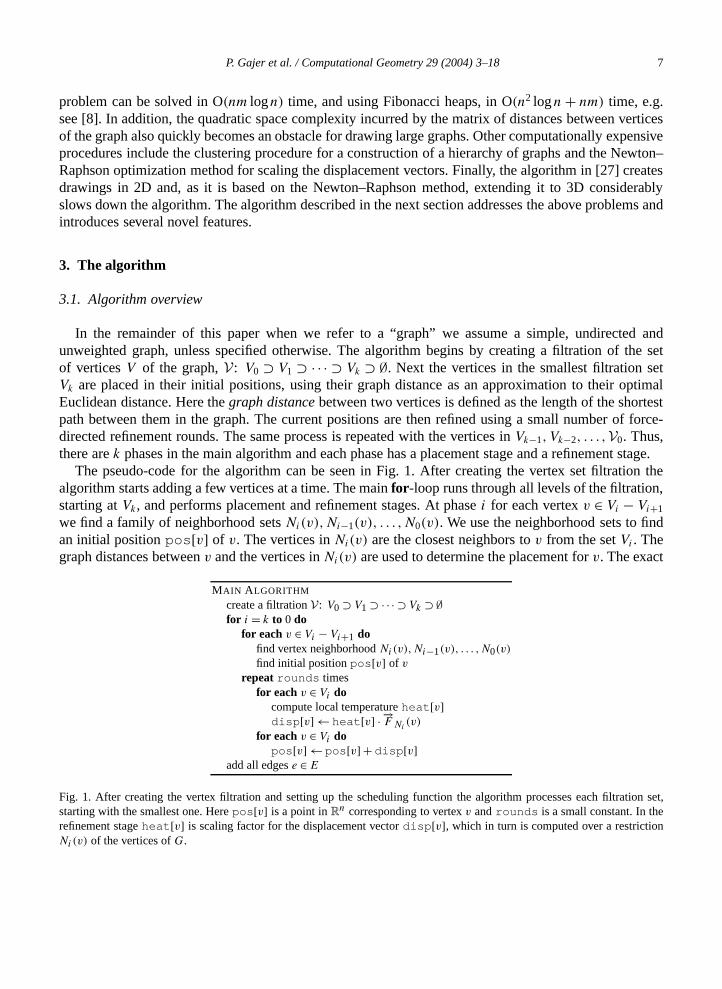
The pseudo-code for the algorithm can be seen in Fig. 1. After creating the vertex set filtratalgorithm starts adding a few vertices at a time. The mainfor-loop runs through all levels of the filtrationstarting atVk, and performs placement and refinement stages. At phasei for each vertexv ∈ Vi − Vi+1

we find a family of neighborhood setsNi(v),Ni−1(v), . . . ,N0(v). We use the neighborhood sets to fian initial positionpos[v] of v. The vertices inNi(v) are the closest neighbors tov from the setVi . Thegraph distances betweenv and the vertices inNi(v) are used to determine the placement forv. The exact

MAIN ALGORITHM

create a filtrationV: V0 ⊃ V1 ⊃ · · · ⊃ Vk ⊃ ∅for i = k to 0 do

for each v ∈ Vi − Vi+1 dofind vertex neighborhoodNi(v),Ni−1(v), . . . ,N0(v)

find initial positionpos[v] of v

repeat rounds timesfor each v ∈ Vi do

compute local temperatureheat[v]disp[v] ← heat[v] · −→

F Ni(v)

for each v ∈ Vi dopos[v] ← pos[v] + disp[v]

add all edgese ∈ E

Fig. 1. After creating the vertex filtration and setting up thescheduling function the algorithm processes each filtrationstarting with the smallest one. Herepos[v] is a point inR

n corresponding to vertexv androunds is a small constant. In threfinement stageheat[v] is scaling factor for the displacement vectordisp[v], which in turn is computed over a restrictioNi(v) of the vertices ofG.


at, just after

ng theed

l

t vector

tings of the

n with

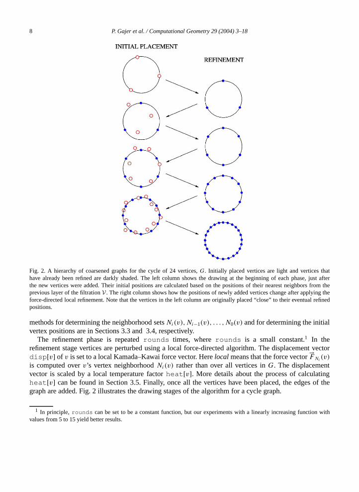
Fig. 2. A hierarchy of coarsened graphs for the cycle of 24 vertices,G. Initially placed vertices are light and vertices thhave already been refined are darkly shaded. The left column shows the drawing at the beginning of each phasethe new vertices were added. Their initial positions are calculated based on thepositions of their nearest neighbors from theprevious layer of the filtrationV . The right column shows how the positions of newly added vertices change after applyiforce-directed local refinement. Note that the vertices in the left column are originally placed “close” to their eventual refinpositions.

methods for determining the neighborhood setsNi(v),Ni−1(v), . . . ,N0(v) and for determining the initiavertex positions are in Sections 3.3 and 3.4, respectively.

The refinement phase is repeatedrounds times, whererounds is a small constant.1 In therefinement stage vertices are perturbed using a local force-directed algorithm. The displacemendisp[v] of v is set to a local Kamada–Kawai force vector. Herelocal means that the force vector

−→FNi

(v)

is computed overv’s vertex neighborhoodNi(v) rather than over all vertices inG. The displacemenvector is scaled by a local temperature factorheat[v]. More details about the process of calculatheat[v] can be found in Section 3.5. Finally, once all the vertices have been placed, the edgegraph are added. Fig. 2 illustrates the drawing stages of the algorithm for a cycle graph.

1 In principle,rounds can be set to be a constant function, but our experiments with a linearly increasing functiovalues from 5 to 15 yield better results.


3.2. Vertex set filtrations

When trying to draw a large graph, it is natural to associate with it a hierarchy of graphs and produceso that

re thanlevel isg. linearber of

ibutiontainingmore

number,graphs,

or the

center

s the GC

rchies,tex set.

depthtested

ohe

the drawing starting with the smallest graph in the hierarchy and drawing larger and larger graphsat each stage we use the previous drawing. Two important properties of such a hierarchy are:

• the depth of the hierarchy (number of levels),• the distribution of the vertices in the levels.

A shallow hierarchy (e.g. constant depth) implies that as we go from one level to the next, moa constant fraction of the vertices are added. Usually this means that information from the oldnot sufficient to create a good drawing on the new level. On the other hand, a deep hierarchy (e.in the number of vertices) is too time consuming to traverse. Thus, logarithmic depth in the numvertices is highly desirable.

The effectiveness of a multi-scale scheme like this also depends on the uniformity of the distrof the vertices at all levels of the hierarchy. The hierarchy of graphs can be thought of as condifferent levels of abstraction of the underlying graph. Uniform distribution of the vertices impliesaccurate levels of abstraction which in turn implies better drawings on each level.

Hadany and Harel [26] create a hierarchy of graphs based on the cluster number, the degreeand the homotopic number. Harel and Koren [27] use a simpler method to create the hierarchy ofwhich relies on thek-clusters problem. Since solving thek-clusters problem or the relatedk-centersproblem is NP-hard [25,28], their algorithm uses a straightforward 2-approximation algorithm fk-centers problem to create a GC filtration. The algorithm begins by producing agraph centers(GC)filtration V = V0 ⊃ V1 ⊃ · · · ⊃ Vk ⊃ ∅ of the setV of vertices of the graphG, with |Vi| = c · xk−i , wherex > 1 andc = |Vk| is a constant. A cluster of vertices closest to each center is created for eachand on every level. A set of weighted edges is computed between elements ofVi , so that the weightscorrespond to the number of edges between the elements of the corresponding clusters. Thufiltration together with the edges forms a hierarchy of graphs.

The creation of a GC filtration proceeds as follows. Pick a random elementv of V and add it toVk.Find a vertex farthest away from all the vertices inVk and add it toVk. Continue this process untilVk

hasc elements. Suppose we have already foundVi , 1 � i � k. To find the next setVi−1 let Vi−1 = Vi

and again continue adding toVi−1 the elements that are farthest away fromVi−1 until |Vi−1| = c · xk−i+1.WhenV1 is completed we have a GC filtration ofV .

While having proper graphs on each level is necessary in many applications utilizing graph hierain the context of graph drawing we can save time and space by using just a filtration of the verNote that in a filtration there are no edges but only vertices. As we already pointed out, logarithmicand “uniform” filtrations are highly desirable for graph drawing purposes. We have developed andone specific such filtration that we call amaximal independent set(MIS) filtration and we use it in thisalgorithm.

Recall thatS ⊂ V is anindependent setof a graphG = (V ,E) if no two elements ofS are connectedby an edge ofG. Equivalently,S is an independent set ofG if the graph distance between any twelements ofS is at least two. Recall that thegraph distancebetween two vertices is the length of tshortest path between them in the graph. A maximal independent set filtration ofG is a family of sets


e

nt setsxan

ces

set

fn

mber ofenters

d space,

tage of

adratic

aldeally,ex

Fig. 3. An example of a MIS filtration. Here the underlying graphG = (V ,E) is a rectangular mesh of size 10× 10. The darkvertices are included in the filtration. HereV = V0, V1 is a standard maximal independent set,V2 is a maximal subset ofV1 sothat the distances between its elements are at least 22 = 4, and so on.

V = V0 ⊃ V1 ⊃ · · · ⊃ Vk ⊃ ∅, such that eachVi is a maximal subset ofVi−1 for which the graph distancbetween any pair of its elements is greater than or equal to 2i ; see Fig. 3.

Since the maximum independent set problem is NP-hard [24], we use maximal independeinstead. Conceptually, MIS filtrations can be constructed as follows. LetV ∗ = V , take a random vertev ∈ V ∗ and add it toV1. Removev and all of its neighbors fromV ∗ and repeat until no more vertices cbe chosen. Suppose we constructed an orderi independent setVi of G. To constructVi+1 let V ∗ = Vi

and take a random vertexv ∈ V ∗ out ofV ∗, and place it inVi+1. Next remove fromV ∗ all vertices whosegraph distance tov is less than or equal to 2i . This distance factor is important in ensuring that vertiare well distributed and in guaranteeing small depth of the filtration. Choose another elementw of V ∗,and remove fromV ∗ the chosen vertex and all vertices whose distance tow is less than or equal to 2i .Placew in Vi+1. Repeat this procedure untilV ∗ is empty. An example of a maximal independentfiltration is shown in Fig. 3.

The construction of a MIS filtration stops at levelk so that 2k > δ(G), whereδ(G) is the diameter oG. Therefore, each MIS filtration has depth O(logδ(G)). MIS filtrations provide excellent distributioof the vertices by construction, a property needed for high quality filtrations.

The three different filtrations considered have their advantages and disadvantages. The nuvertices in the MIS filtration sets is controlled by the topology of the graph, whereas in the graph cfiltration the sizes are arbitrarily set by the user. While we cannot guarantee sub-quadratic time anMIS filtrations are faster to create and use very little space compared to GC filtrations.

3.3. Finding vertex neighborhoodsNi(v)

One of the key ideas of the hierarchical force-directed graph layout method is that at each sthe construction a force-directed position refinement method is applied to a given layerVi of a filtrationonly locally. More precisely, for a given energy functionE andv ∈ Vi , the gradient ofE at pos[v] iscomputed not forE but for the restriction ofE to some neighborhoodNi(v) of v in Vi . A good filtrationof V and an efficient local position refinement strategy are the key means of achieving a sub-qulower bound for space and time complexity of our method.

This section describes a procedure of constructing the neighborhood sets,Ni(v), and the definitionof the functionnbrs(i) which determines the size ofNi(v). Intuitively, each stage of the hierarchicgraph drawing strategy should result in a closer approximation of the final drawing of the graph. Iat the last stage, when we perform a force-directed local refinement of the position of each vertv of


the graph, it should be enough to takeN0(v) to be the set of adjacent vertices ofv. The time complexityof this last stage calculation is∑

awing

set

n

A newps

n

c ·v∈V

N0(v) = c · n · avgDeg(G),

whereavgDeg(G) is the average degree ofG and c is a constant. We would like to makec · n ·avgDeg(G) an upper bound for the complexity of calculations at each stage of graph drconstruction. Therefore, we set

nbrs(i) = �

(avgDeg(G) · n

|Vi|)

.

SupposeV is a logarithmic depth filtration of the setV of vertices ofG. The calculation of the setNk(v),Nk−1(v), . . . ,N0(v) is performed for each elementv ∈ V only once, when it is added to a sof already placed vertices; see Fig. 1. We require thatNi(v) contains�(nbrs(i)) elements for eachi = k, k − 1, . . . ,0. Therefore, the space complexity of this strategy is bounded above by

k∑i=0

|Vi − Vi+1|(nbrs(1) + nbrs(2) + · · · + nbrs(i)

). (1)

SinceVi+1 ⊂ Vi , we have|Vi − Vi+1| = |Vi| − |Vi+1|, and after simplifications, (1) takes the form

k∑i=0

|Vi|nbrs(i) � c0

k∑i=0

|Vi|avgDeg(G) · n|Vi| = c0

k∑i=0

avgDeg(G) · n

= c0avgDeg(G) · (k + 1)n. (2)

Similarly we can show that there exists a positive constantc1 so that Eq. (1) is greater thac1avgDeg(G) · (k + 1)n. Thus, the storage complexity of the above strategy for findingNk(v),Nk−1(v),

. . . ,N0(v) for all v ∈ V is �(avgDeg(G)kn). If G is of bounded degree, then�(avgDeg(G)kn) =�(kn), wherek = logn for a GC filtration, andk = logδ(G) for a MIS filtration.

Let thedepth of a vertex, depth(v), with respect toV be the largestd, such thatv ∈ Vd . The setsNk(v),Nk−1(v), . . . ,N0(v) are created by repeated application of a breadth-first search algorithm.vertex with depthd is placed in each ofNj(v), for j � d, if Nj(v) is not already full. The process stowhen allNj(v)s are full. Note that the running time of this procedure is bounded above by

k∑i=1

|Vi|(1 · nbrs(1) + 2 · nbrs(2) + · · · + i · nbrs(i)

). (3)

As in the case of the expression (1), (3) is equal to

k∑i=0

i|Vi|nbrs(i) � c0

k∑i=0

i|Vi |avgDeg(G) · n|Vi| = c0

k∑i=0

iavgDeg(G) · n

= c0avgDeg(G) · (k + 1)k

2n. (4)

Similarly we can show that there exists a positive constantc1 so that Eq. (3) is greater thac1avgDeg(G) · (k+1)k

2 n. The time complexity of this strategy for findingNk(v),Nk−1(v), . . . ,N0(v) for


all v ∈ V is �(avgDeg(G)k2n). If G is of bounded degree, then�(avgDeg(G)k2n) = �(k2n), wherek = logn for a GC filtration, andk = logδ(G) for a MIS filtration.

planecurrentprocess

te

e startby

eeedway tow vertex

gy on this

e

n

are usedrsable

airs of

3.4. Initial placement of vertices

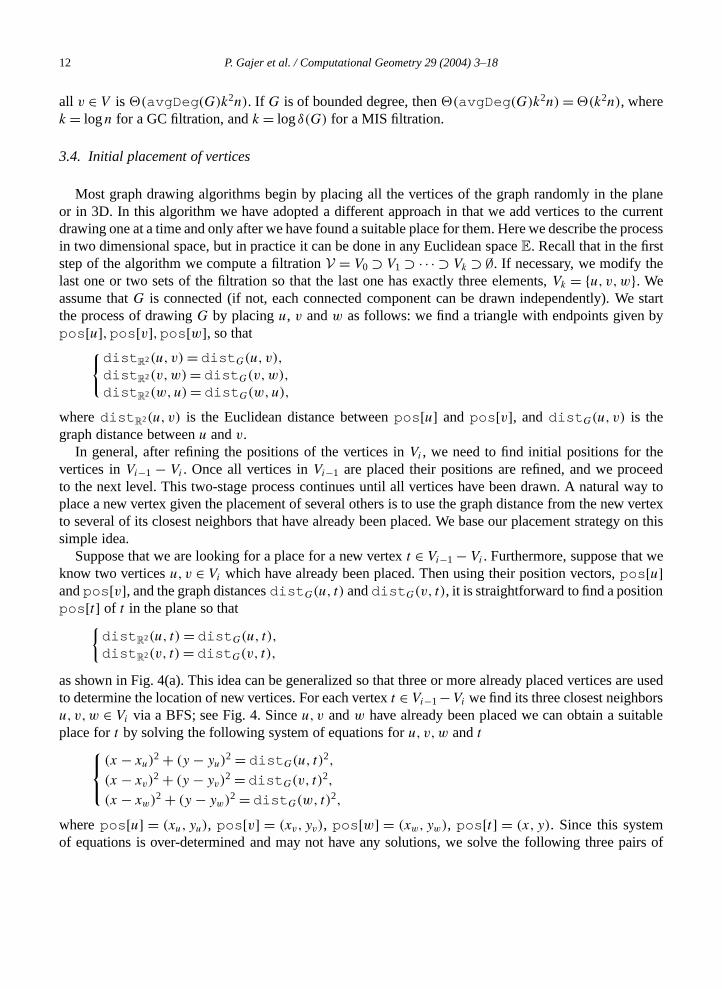
Most graph drawing algorithms begin by placing all the vertices of the graph randomly in theor in 3D. In this algorithm we have adopted a different approach in that we add vertices to thedrawing one at a time and only after we have found a suitable place for them. Here we describe thein two dimensional space, but in practice it can be done in any Euclidean spaceE. Recall that in the firsstep of the algorithm we compute a filtrationV = V0 ⊃ V1 ⊃ · · · ⊃ Vk ⊃ ∅. If necessary, we modify thlast one or two sets of the filtration so that the last one has exactly three elements,Vk = {u, v,w}. Weassume thatG is connected (if not, each connected component can be drawn independently). Wthe process of drawingG by placingu, v andw as follows: we find a triangle with endpoints givenpos[u],pos[v],pos[w], so that{distR2(u, v) = distG(u, v),

distR2(v,w) = distG(v,w),

distR2(w,u) = distG(w,u),

wheredistR2(u, v) is the Euclidean distance betweenpos[u] andpos[v], anddistG(u, v) is thegraph distance betweenu andv.

In general, after refining the positions of the vertices inVi , we need to find initial positions for thvertices inVi−1 − Vi . Once all vertices inVi−1 are placed their positions are refined, and we procto the next level. This two-stage process continues until all vertices have been drawn. A naturalplace a new vertex given the placement of several others is to use the graph distance from the neto several of its closest neighbors that have already been placed. We base our placement stratesimple idea.

Suppose that we are looking for a place for a new vertext ∈ Vi−1 − Vi . Furthermore, suppose that wknow two verticesu, v ∈ Vi which have already been placed. Then using their position vectors,pos[u]andpos[v], and the graph distancesdistG(u, t) anddistG(v, t), it is straightforward to find a positiopos[t] of t in the plane so that{

distR2(u, t) = distG(u, t),

distR2(v, t) = distG(v, t),

as shown in Fig. 4(a). This idea can be generalized so that three or more already placed verticesto determine the location of new vertices. For each vertext ∈ Vi−1−Vi we find its three closest neighbou, v,w ∈ Vi via a BFS; see Fig. 4. Sinceu, v andw have already been placed we can obtain a suitplace fort by solving the following system of equations foru, v,w andt

(x − xu)

2 + (y − yu)2 = distG(u, t)2,

(x − xv)2 + (y − yv)

2 = distG(v, t)2,

(x − xw)2 + (y − yw)2 = distG(w, t)2,

wherepos[u] = (xu, yu), pos[v] = (xv, yv), pos[w] = (xw, yw), pos[t] = (x, y). Since this systemof equations is over-determined and may not have any solutions, we solve the following three p


ose the

f thean in ther mostlacedlligentilar to

ebuteraturer.

wton–ges in

not be

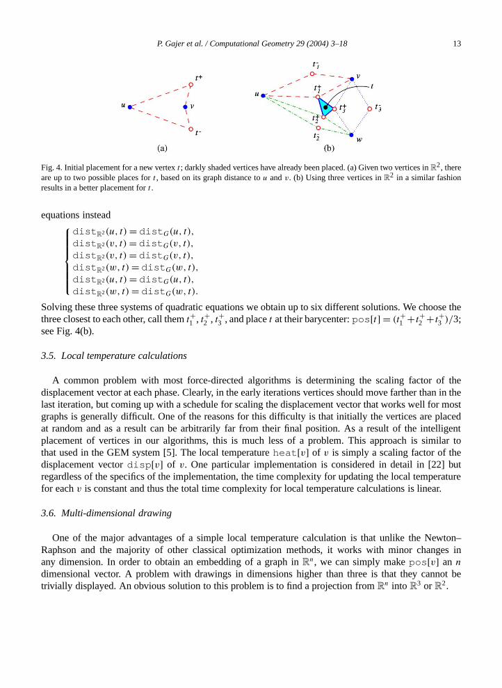
Fig. 4. Initial placement for a new vertext ; darkly shaded vertices have already been placed. (a) Given two vertices inR2, there

are up to two possible places fort , based on its graph distance tou andv. (b) Using three vertices inR2 in a similar fashionresults in a better placement fort .

equations instead




distR2(w, t) = distG(w, t),


distR2(w, t) = distG(w, t).

Solving these three systems of quadratic equations we obtain up to six different solutions. We chothree closest to each other, call themt+1 , t+2 , t+3 , and placet at their barycenter:pos[t] = (t+1 + t+2 + t+3 )/3;see Fig. 4(b).

3.5. Local temperature calculations

A common problem with most force-directed algorithms is determining the scaling factor odisplacement vector at each phase. Clearly, in the early iterations vertices should move farther thlast iteration, but coming up with a schedule for scaling the displacement vector that works well fographs is generally difficult. One of the reasons for this difficulty is that initially the vertices are pat random and as a result can be arbitrarily far from their final position. As a result of the inteplacement of vertices in our algorithms, this is much less of a problem. This approach is simthat used in the GEM system [5]. The local temperatureheat[v] of v is simply a scaling factor of thdisplacement vectordisp[v] of v. One particular implementation is considered in detail in [22]regardless of the specifics of the implementation, the time complexity for updating the local tempfor eachv is constant and thus the total time complexity for local temperature calculations is linea

3.6. Multi-dimensional drawing

One of the major advantages of a simple local temperature calculation is that unlike the NeRaphson and the majority of other classical optimization methods, it works with minor chanany dimension. In order to obtain an embedding of a graph inR

n, we can simply makepos[v] an n

dimensional vector. A problem with drawings in dimensions higher than three is that they cantrivially displayed. An obvious solution to this problem is to find a projection fromR

n into R3 or R

2.


Consider the case in which a four dimensional drawing is projected down to three dimensions. Theprojection method described below generalizes to higher dimensions as well. We begin by taking arandom vectore′

0 in R4 and normalizing ite0 = e′

0/‖e′0‖. Next we find three vectorse′

1,e′2,e

′3 ∈ R

4

g ars. We

e

fs

l basisal

fromoebiusD and

so thate0, e′1, e′

2, e′3 are linearly independent inR4. We find these vectors by repeatedly choosin

random vector and checking if it is independent from the previous ones until we have four vectothen use the Gram–Schmidt orthogonalization process to produce an orthonormal basise0, e1, e2, e3 ofR

4 usinge0, e′1, e′

2, e′3. The three vectorse1, e2, e3 span a three-dimensional subspaceS of R

4 whichis perpendicular to the vectore0. The orthogonal projectionρ :R4 → S from R

4 ontoS in the directionof the vectore0 is given by the formula

ρ(v) = v − (e0, v) ∗ e0,

where(e0, v) is the scalar product betweene0 andv. Yet to displayv on the screen using OpenGL, wneed the coordinates(v1, v2, v3) of the projectionρ(v) of v ontoS with respect to the basis vectorse1,e2, e3. We get these by a simple scalar product calculationv1 = (e1, v), v2 = (e2, v), v3 = (e3, v).

The above procedure easily generalizes to higher dimensions. For anym > 3, we find a projection oR

m onto some three-dimensional subspaceS of Rm by specifyingm − 3 linearly independent vector

e′0,e

′1, . . . ,e

′m−4 (generalized projection directions), and complete them to a basise′

0,e′1, . . . ,e

′m−1

of Rm. Next, using the Gram–Schmidt orthogonalization process we create an orthonorma

e0,e1, . . . ,em−1 of Rm. The last three vectorsem−3, em−2, em−1 form a basis of a three-dimension

subspaceS of Rm, and the coordinates(v1, v2, v3) of the orthogonal projection of anyv ∈ R

m ontoS aregiven by the formulav1 = (em−3, v), v2 = (em−2, v), v3 = (em−3, v).

Our experiments with four dimensional drawings yield results that are noticeably differentregular three dimensional drawings. In particular, note the problems with the drawings of the Mstrip directly in 3D in Fig. 5 and the much better quality drawings of the same graphs drawn in 4projected to 3D in Fig. 6.

Fig. 5. Moebius strips on 150, 300 and 1500 vertices drawn in directly 3D. Note the rough “twists”.

Fig. 6. The same Moebius strips as in Fig. 5 but drawn in 4D and projected in 3D. Note the smooth twists.


3.7. Space and time complexity

Main Theorem. If G is a graph of bounded degree andV is a GC filtration or a MIS filtration of the

e andd

vertexrithme of thecreation

bed

setV of vertices ofG, then the time complexity of our algorithm, after constructingV , is �(n · k2) andthe space required is�(n · k), wherek = logn if V is a GC filtration, andk = logδ(G) if V is a MISfiltration.

Proof. The proof of the theorem follows from the fact that after building a filtrationV , all parts ofthe algorithm take linear time and space, except the procedure for findingNk(v),Nk−1(v), . . . ,N0(v) foreach elementv of V . Thus both time and space complexity of the algorithm is determined by the timspace complexity of the procedure for finding the neighborhood setsNi(v). In Section 3.3, we showethat the time required for finding the setsNi(v) is �(n · k2) and the space required is�(n · k), whichconcludes the proof. �

4. Conclusion and future work

We have presented a novel algorithm for drawing large graphs. The algorithm employs afiltration together with intelligent placement of vertices and fast energy minimization. The algoproduces drawings in two, three and higher dimensions in sub-quadratic time and space. Onproblems that remains to be addressed concerns the running time and space complexity for the

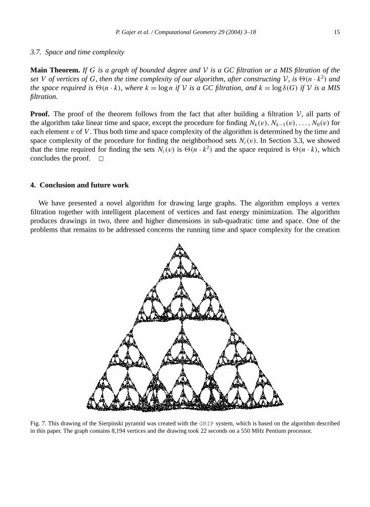
Fig. 7. This drawing of the Sierpinski pyramid was created with theGRIP system, which is based on the algorithm descriin this paper. The graph contains 8,194 vertices and the drawing took 22 seconds on a 550 MHz Pentium processor.


of the maximal independent set filtration. While our tests indicate that the running time and space requiredare sub-quadratic in the number of vertices in the graph, this remains to be proved. While the algorithmworks very well for sparse graphs and graphs of low degree, it does not produce high quality drawings

ificantgraphs.

mes theand

ampleof the

m

ort.Drawing

. Phys.

posium

Human

the 3rdp. 162–

–331.rentice

J. Graph

Drawing

ingsBerlin,

for all graphs. In particular, well-connected graphs and graphs with small diameter pose signchallenges as the vertex filtrations become very shallow. Also, our algorithm works best on sparseWhile the majority of large graphs that need to be visualized have low average degree, sometimaximum degree can be as big as O(n). An algorithm for general graphs with sub-quadratic timespace complexity would be highly desirable.

The algorithm described in this paper is used in the design of theGRIP system (Graph dRawing withIntelligentPlacement) [22] which produced the drawings in Figs. 5 and 6. We include one more exof an interesting class of graphs called Sierpinski graphs. The drawing of the Sierpinski pyramid6th order, which contains 8194 vertices, was produced usingGRIP in 22 seconds on a 550 MHz Pentiuprocessor; see Fig. 7.

Acknowledgements

We would like to thank the anonymous referees for the useful comments and suggestions.

References

[1] J. Barnes, P. Hut, A hierarchical O(N logN ) force calculation algorithm, Nature 324 (1986) 446–449. Technical Rep[2] T.C. Biedl, Three approaches to 3D-orthogonal box-drawings, in: Proceedings of the 6th Symposium on Graph

(GD), in: Lecture Notes in Computer Science, vol. 1547, Springer-Verlag, Berlin, 1998, pp. 30–43.[3] A. Brandt, Multilevel computations of integral transforms and particle interactions with oscillatory kernels, Comput

Comm. 65 (1991) 24–38.[4] A. Brandt, Multigrid methods in lattice field computations, Nucl. Phys. B26 (1992) 137–180. Proc. Suppl.[5] I. Bruß, A. Frick, Fast interactive 3-D graph visualization, in: F.J. Brandenburg (Ed.), Proceedings of the 3rd Sym

on Graph Drawing (GD), Lecture Notes Computer Science, vol. 1027, Springer-Verlag, Berlin, 1996, pp. 99–110.[6] J.D. Cohen, Drawing graphs to convey proximity: An incremental arrangement method, ACM Trans. Computer–

Interaction 4 (3) (1997) 197–229.[7] R.F. Cohen, P. Eades, T. Lin, F. Ruskey, Three-dimensional graph drawing, Algorithmica 17 (1997) 199–208.[8] T.H. Cormen, C.E. Leiserson, R.L. Rivest, Introduction to Algorithms, MIT Press, Cambridge, MA, 1990.[9] I.F. Cruz, J.P. Twarog, 3d graph drawing with simulated annealing, in: F.J. Brandenburg (Ed.), Proceedings of

Symposium on Graph Drawing (GD), Lecture Notes Computer Science, vol. 1027, Springer-Verlag, Berlin, 1996, p165.

[10] R. Davidson, D. Harel, Drawing graphics nicely using simulated annealing, ACM Trans. Graph. 15 (4) (1996) 301[11] G. Di Battista, P. Eades, R. Tamassia, I.G. Tollis, Graph Drawing: Algorithms for the Visualization of Graphs, P

Hall, Englewood Cliffs, NJ, 1999.[12] C.A. Duncan, M.T. Goodrich, S.G. Kobourov, Balanced aspect ratio trees and their use for drawing large graphs,

Alg. Appl. 4 (2000) 19–46.[13] P. Eades, A heuristic for graph drawing, Congr. Numer. 42 (1984) 149–160.[14] P. Eades, Q. Feng, Multilevel visualization of clustered graphs, in: Proceedings of the 4th Symposium on Graph

(GD), Lecture Notes in Computer Science, vol. 1190, Springer-Verlag, Berlin, 1996, pp. 101–112.[15] P. Eades, Q. Feng, X. Lin, Straight-line drawing algorithmsfor hierarchical graphs and clustered graphs, in: Proceed

of the 4th Symposium on Graph Drawing (GD), Lecture Notes in Computer Science, vol. 1190, Springer-Verlag,1996, pp. 113–128.


[16] P. Eades, A. Symvonis, S. Whitesides, Two algorithms for three dimensional orthogonal graph drawing, in: S. North (Ed.),Proceedings of the 4th Symposium on Graph Drawing (GD), Lecture Notes in Computer Science, vol. 1190, Springer-Verlag, Berlin, 1996, pp. 139–154.

oftware

rence on

s.),pringer-

9–1164.ems

Notes in

ew

93–306.and

raph

33 (3)

Dept. of

l. 2025,

s of, 1995,

93-3E,

irectedl. 1027,

castle,

h, 1997,

sium on.rsity of

uits and

Trans.

[17] Q. Feng, Algorithms for drawing clustered graphs, PhD Thesis, Department of Computer Science and SEngineering, University of Newcastle, 1997.

[18] Q. Feng, R.F. Cohen, P. Eades, How to draw a planar clustered graph, in: Proc. 1st Annual International ConfeComputing and Combinatorics (COCOON ’95), 1995, pp. 21–31.

[19] A. Frick, A. Ludwig, H. Mehldau, A fast adaptive layout algorithm for undirected graphs, in: R. Tamassia, I.G. Tollis (EdProceedings of the 2nd Symposium on Graph Drawing (GD), Lecture Notes in Computer Science, vol. 894, SVerlag, Berlin, 1995, pp. 388–403.

[20] T. Fruchterman, E. Reingold, Graph drawing by force-directed placement, Softw. – Pract. Exp. 21 (11) (1991) 112[21] G.W. Furnas, Generalized fisheye views, in: Proceedings of ACM Conference on Human Factors in Computing Syst

(CHI’86), 1986, pp. 16–23.[22] P. Gajer, S.G. Kobourov, GRIP: Graph dRawing with Intelligent Placement, J. Graph Alg. Appl. 6 (3) (2002) 203–224.[23] E.R. Gansner, S.C. North, Improved force-directed layouts, in: Lecture Notes in Computer Science, Lecture

Computer Science, vol. 1547, Springer-Verlag, Berlin, 1998, pp. 364–373.[24] M.R. Garey, D.S. Johnson, Computers and Intractability: A Guide to the Theory of NP-Completeness, Freeman, N

York, 1979.[25] T.F. Gonzalez, Clustering to minimize the maximum intercluster distance, Theoret. Comput. Sci. 38 (2–3) (1985) 2[26] Hadany, D. Harel, A multi-scale algorithm for drawing graphs nicely, DAMATH: Discrete Applied Mathematics

Combinatorial Operations Research and Computer Science 113 (2001).[27] D. Harel, Y. Koren, A fast multi-scale method for drawinglarge graphs, in: Proceedings of the 8th Symposium on G

Drawing (GD), Lecture Notes in Computer Science, vol. 1984, Springer-Verlag, Berlin, 2000, pp. 183–196.[28] D.S. Hochbaum, D.B. Shmoys, A unified approach to approximate algorithms for bottleneck problems, J. ACM

(1986) 533–550.[29] T. Kamada, S. Kawai, Automatic display of network structures for human understanding, Technical Report 88-007,

Inf. Science, University of Tokyo, 1988.[30] M. Kaufmann, D. Wagner, Drawing Graphs: Methods and Models, Lecture Notes in Computer Science, vo

Springer-Verlag, Berlin, 2001.[31] K. Kaugars, J. Reinfelds, A. Brazma, A simple algorithm for drawing large graphs on small screens, in: Proceeding

the 3rd Symposium on Graph Drawing (GD), Lecture Notes in Computer Science, vol. 894, Springer-Verlag, Berlinpp. 278–281.

[32] S.G. Kobourov, Visualizing large graphs, PhD Thesis, Johns Hopkins University, 2000.[33] K. Misue, K. Sugiyama, An overview of diagram based idea organizer: D-ABDUCTOR, Research Report IIAS-RR-

Fujitsu Laboratories Ltd., 1993.[34] B. Monien, F. Ramme, H. Salmen, A parallel simulated annealing algorithm for generating 3D layouts of und

graphs, in: Proceedings of the 3rd Symposium on Graph Drawing (GD), Lecture Notes in Computer Science, voSpringer-Verlag, Berlin, 1996, pp. 396–408.

[35] D.I. Ostry, Some three-dimensional graph drawing algorithms, Master’s Thesis, University of Newcastle, NewAustralia, 1996.

[36] A. Papakostas, I.G. Tollis, Incremental orthogonal graph drawing in three dimensions, in: Proceedings of the 5tSymposium on Graph Drawing (GD), Lecture Notes in Computer Science, vol. 1353, Springer-Verlag, Berlinpp. 52–63.

[37] A. Quigley, P. Eades, FADE: graph drawing, clustering, and visual abstraction, in: Proceedings of the 8th SympoGraph Drawing (GD), Lecture Notes in Computer Science, vol. 1984, Springer-Verlag, Berlin, 2000, pp. 197–210

[38] A.J. Quigley, Large scale relational information visualization, clustering, and abstraction, PhD Thesis, UniveNewcastle, Australia, 2001.

[39] N. Quinn, M. Breur, A force directed component placement procedure for printed circuit boards, IEEE Trans. CircSystems CAS-26 (6) (1979) 377–388.

[40] M. Sarkar, M.H. Brown, Graphical fisheye views, Comm. ACM 37 (12) (1994) 73–84.[41] K. Sugiyama, K. Misue, Visualization of structural information: Automatic drawing of compound digraphs, IEEE

Systems Man Cybernet. 21 (4) (1991) 876–892.


[42] D. Tunkelang, JIGGLE: Java interactive general graph layout environment, in: Proceedings of the 6th Symposium onGraph Drawing (GD), Lecture Notes in Computer Science, vol. 1547, Springer-Verlag, Berlin, 1998, pp. 413–422.

[43] C. Walshaw, A multilevel algorithm for force-directed graph drawing, in: Proceedings of the 8th Symposium on Graph

edings,

on.

Drawing (GD), Lecture Notes in Computer Science, vol. 1984, Springer-Verlag, Berlin, 2000, pp. 171–182.[44] C. Ware, Information Visualization, Morgan Kaufmann, 2000.[45] C. Ware, D. Hui, G. Franck, Visualizing object oriented software in three dimensions, in: CASCON 1993 Proce

1993.[46] C.D. Wickens, Engineering Psychology and Human Performance, Harper Collins, New York, 1991.[47] D.R. Wood, Multi-dimensional orthogonal graph drawing with small boxes, in: Proceedings of the 7th Symposium

Graph Drawing (GD), Lecture Notes in Computer Science, vol. 1731, Springer-Verlag, Berlin, 1999, pp. 311–322

A multi-dimensional approach to force-directed layouts of ...

Documents

Transcript of A multi-dimensional approach to force-directed layouts of ...