1

Hayashi Spectra of the Northern Hemisphere Mid-latitude Atmospheric Variability in the NCEP and ERA 40 Reanalyses

ALESSANDRO DELL’AQUILA(1), VALERIO LUCARINI(2), PAOLO RUTI(1), AND SANDRO

CALMANTI(1)

1Progetto Speciale Clima Globale, Ente Nazionale per le Nuove Tecnologie, l’Energia e l’Ambiente, Roma, Italy

2Dipartimento di Matematica ed Informatica, Università di Camerino, Camerino (MC), Italy

Abstract

We compare 45 years of the reanalyses of NCEP-NCAR and ECMWF in terms of their

representation of the mid-latitude winter atmospheric variability for the overlapping time

frame 1957-2002. We adopt the classical approach of computing the Hayashi spectra of

the 500 hPa geopotential height fields. Discrepancies are found especially in the first 15

years of the records in the high-frequency-high wavenumber propagating waves and

secondly on low frequency-low wavenumber standing waves. This implies that in the first

period the two datasets have a different representation of the baroclinic available energy

conversion processes. In the period starting from 1973 a positive impact of the aircraft

data on the Euro-Atlantic synoptic waves has been highlighted. Since in the first period

the assimilated data are scarcer and of lower quality than later on, they provide a weaker

constraint to the model dynamics. Therefore, the resulting discrepancies in the reanalysis

products may be mainly attributed to differences in the models’ behavior.

2

1. Introduction

Reanalysis products are designed to obtain global, homogeneous and self-

consistent datasets of the atmospheric dynamics on the longest time scale allowed

by the currently available instrumental data (Kistler et al., 2001). Recently, the

National Center for Environmental Prediction (NCEP), in collaboration with the

National Center for Atmospheric Research (NCAR) (Kistler et al., 2001), and the

European Center for Mid-Range Weather Forecast (ECMWF) (Simmons and

Gibson, 2000) have released re-analysed datasets for the time frames 1948-2004

and 1957-2002, respectively. We henceforth refer to such reanalyses with the

names of NCEP and ERA 40, respectively.

The re-analysed data have been used in a large variety of contexts, ranging from

the direct cross validation with independent observations (Josey, 2001; Renfew et

al., 2002), to the study of specific aspects of atmospheric dynamics (Annamalai et

al., 1999; Hodges et al., 2003), to their usage as external input for the modeling of

other components of the climate system (Harrison et al., 2002; Josey et al., 2002).

Since they represent the best available homogeneous datasets for climate studies

and for validation of climate general circulation models (GCMs), it is of

paramount importance to assess the consistency of these reanalyses in the

representation of the variability of the atmosphere. Moreover, the reanalyses can

presently be considered long enough to allow for the detection of significant

changes (trends) in the climate system. Any robust change in climate occurring on

the time scales of a few decades should be detectable in both reanalyses. The

presence of an overlapping period of almost five decades (1957-2002) between

the NCEP and ERA 40 datasets provides the baseline for intercomparison studies.

In a sense, the assimilation processes employed to produce the two reanalyses are

3

to be envisioned as slightly different dynamically consistent interpolations of

similar data. In this view, the two dataset are expected to provide equivalent

pictures of atmospheric variability and changes. However, the reanalyses differ

under several aspects. The assimilation of data is based upon the use of slightly

modified version of the numerical model employed for operational weather

forecast. The numerical models employed for producing NCEP and ERA 40 differ

mainly in their resolution and in the parameterization of small scale physics. The

resulting discrepancies between the two datasets should be taken into account in

intercomparison studies (Caires et al., 2004; Ruiz-Barradas et al., 2004; Sterl,

2004). Other inhomogeneities which are internal to each of the two dataset may

arise from the unequal spatial and temporal density of instrumental data available

during the period covered by the reanalyses (Kistler et al., 2001). Most

importantly, the assimilation of satellite data has dramatically improved the

quality of the reanalyses over the last three decades (Sturaro, 2003). Sterl (2004),

analyzing monthly averaged variables, showed that the two reanalyses differ the

most where less instrumental data are available (i.e. in the southern hemisphere).

In the work of Sterl (2004), no significant difference is reported in the northern

hemisphere. However, large inhomogeneities exist in the spatial and temporal

distribution of data, even in the northern hemisphere. Therefore, discrepancies

may exist between the two reanalyses which are not captured within the low time

resolution employed by Sterl (2004).

In this work, we reconsider the differences observed in the mid-latitude northern

hemispheric winters observed in the NCEP and ERA 40 reanalyses by allowing

for a time resolution of one day.

4

We use classical space time Fourier decomposition techniques to characterize the

discrepancies in the 500hPa geopotential height fields provided by the two

reanalyses.

Theoretical and observational arguments suggest that two main features of mid-

latitude northern hemispheric winter variability can be somewath unambiguously

separated, both in terms of signal and physical processes (Benzi et al., 1986).

The synoptic phenomena are traveling waves characterized by time scales of the

order of 2-7 days and by spatial scales of the order of few thousands kilometers,

and can be associated with release of available energy driven by conventional

baroclinic conversion (Blackmon, 1976; Speranza, 1983 Wallace et al, 1988). At

lower frequencies, (period of 10-40 days) the variability is mostly due to the

dynamics of long stationary waves, locked by orography (Charney and Straus,

1980; Hansen and Sutera, 1983; Buzzi et al. 1984; Benzi et al., 1986).

Building upon this conceptual framework, we first measure the difference

between the two reanalyses in the spectral space explored by means of the

Hayashi decomposition (Hayashi, 1971, 1979; Pratt, 1976; Fraedrich and Bottger,

1978) into standing and traveling waves. Then, we suggest some possible

explanation based on actual observations of the 500hPa geopotential height field

and of our knowledge of the assimilation process.

This study is also a preliminary test for some of the methodologies and

diagnostics tools which will be employed in the broader context of a sub-

diagnostic project presented to the Program for Climate Model Diagnosis and

Intercomparison (PCMDI), sponsored by the Intergovernmental Panel on Climate

Change Assessment Report 4 (IPCC-AR4).

The paper is organized as follows. In section 2 we describe the data and how

spectral methods can be used to select the latitudinal band relevant for mid-

5

latitudes atmospheric variability. In section 3 we show the results of Hayashi

spectral analysis for the two datasets and discuss the emerging differences. In

section 4 we compare the variability of the 500hPa geopotential height fields for

the two datasets before and after the onset of satellites observations. In section 5

we present our conclusions and outlook on future studies.

6

2. Data and methods

The 500hPa geopotential height is the most relevant variable descriptive of the

large scale atmospheric circulation (Holton, 1992). Therefore, it constitutes a

fundamental benchmark for the comparison of different atmospheric datasets of

climatological relevance. We use the freely available northern hemisphere 500hPa

geopotential height reanalysis provided by the NCEP and ERA 40 datasets. We

consider the datasets for the overlapping time frame ranging from September 1st

1957 to August 31st 2002. Both reanalyses are publicly released with spatial

resolution of 2.5° x 2.5°, with a resulting effective horizontal grid of 144 x 73

points. The maximum time resolution is six hours. However, in order to focus on

time scales longer than one day, for both reanalyses we consider daily data,

obtained by arithmetically averaging the available 4 times daily data.

Our study focuses on the northern hemisphere mid-latitude atmospheric winter

variability. To this aim, we follow Benzi and Speranza (1989) and select the

December-January-February (DJF) data relative to the latitudinal belt 30°N-75°N

where the bulk of the baroclinic and of the low frequency planetary waves activity

is observed. We average day wise the geopotential field over such latitudinal belt

in order to derive a one dimensional longitudinal field representative of the

atmospheric variability in the mid-latitudes.

The variability of the one dimensional field in terms of waves of different periods

and wavelengths can be effectively described by means of the space-time Fourier

decomposition introduced by Hayashi (1971, 1979). By computing the cross-

spectra and the coherence of the signal, such method allows for a separation of the

eastward and westward wave propagating components from the standing

component. In the Appendix we present a full account of this methodology.

7

3. Hayashi spectra

3a. Climatological average

Figures 1a-1d show the various components of the 45-winters averages of the

Hayashi spectra as computed from the NCEP reanalysis dataset. The spectra

express the energy density of the wave field with respect to frequency and

wavenumber and its decomposition into standing and propagating components.

Figure 1a shows ( )ω,kHT , the total energy spectrum, figure 1b shows ( )ω,kHS ,

the energy spectrum related to standing waves, figure 1c shows ( )ω,kHE , the

energy spectrum related to eastward propagating waves, and figure 1d shows

( )ω,kHW , the energy spectrum of the westward propagating waves. The overbar

indicates the operation of averaging over the N=45 winters. Throughout the paper,

the indexes T, S, E, and W indicate total, standing and eastward/westward

propagating components, respectively. As customary in literature, the Hayashi

spectra have been obtained by multiplying the energy spectra by πω 2⋅k , in

order to compensate for the non-constant density of points in a log-log plot (see

Appendix A).

A large portion of the total energy is concentrated in the low frequency – low

wavenumber domain, and can be related mostly to standing waves and to

westward propagating waves, as can be deduced from figures 1b and 1d. The high

frequency - small wavelength domain, corresponding mainly to synoptic

disturbances, contains a smaller portion of the total energy, and is essentially

related to eastward propagating waves. The fact that eastward propagating waves

are essentially characterized by short wavelength and that long wavelengths

8

characterize westward propagating waves is consistent with the Rossby waves

picture. Accordingly, in figure 1c we observe that it is possible to recognize the

frame of a monotonic dispersion relation ( )kωω = for eastward propagating

waves. Instead, in figure 1d the appearance of a dispersion relation for westward

propagating waves is unclear. These results have a good agreement with the past

analyses performed along the same lines (Fraedrich and Bottger, 1978; Speranza,

1983).

A first insight of the discrepancies between the two reanalyses can be gained by

considering the difference between the two mean Hayashi spectra, portrayed in

figures 2a-2d.

When considering the difference of the two total energy spectra (figure 2a), major

discrepancies can be observed in the high-frequency range, corresponding to

synoptic, eastward propagating disturbances. This feature is confirmed in Fig. 2c

where a significant discrepancy is observed in this component of the Hayashi

decomposition. Instead, no significant difference is found in the westward

propagating signal (figure 2d).

When considering the difference spectrum of the standing waves energy (figure

2b), we observe that the most significant contribution comes from the low

frequency-low wavenumber sector. In particular, large differences are observed

for wavenumbers ranging from 3 to 5, and for periods longer than 20 days. In this

domain we do not observe large discrepancies for the total energy spectra. This

implies that the two datasets should differ in the repartition of the energy between

standing and traveling waves.

Such disagreements are quite impressive because the Hayashi spectra have been

averaged over the 45 winters, thus proving that the climatology of the winter

atmospheric variability of the two datasets is not fully equivalent.

9

3b. Interannual variability

In this paragraph we inspect the temporal behavior of the previously observed

discrepancies by considering specific spectral subdomains. We introduce the

following integral quantities:

(1) ( ) ( )∫ ∫=Ω2

1

2

1

, ω

ω

ωωk

k

nj

nj kHdkdE , with j=T,S,E,W;

where n indicates the year. The integration extremes, 2/1ω and 2/1k , determine the

spectral region of interest [ ] [ ]2121 ,, kk×=Ω ωω . The quantity ( )ΩnjE introduced in

equation (1) represents the fraction of energy of the full spectrum associated to a

given subdomain Ω and to a given year n. Therefore, for various choices of Ω ,

the comparison of the quantities ( )ΩnjE obtained from the two reanalyses can help

identifying differences in the capability of describing processes occurring on a

given spatial and temporal scale and pertaining to qualitatively different physical

processes.

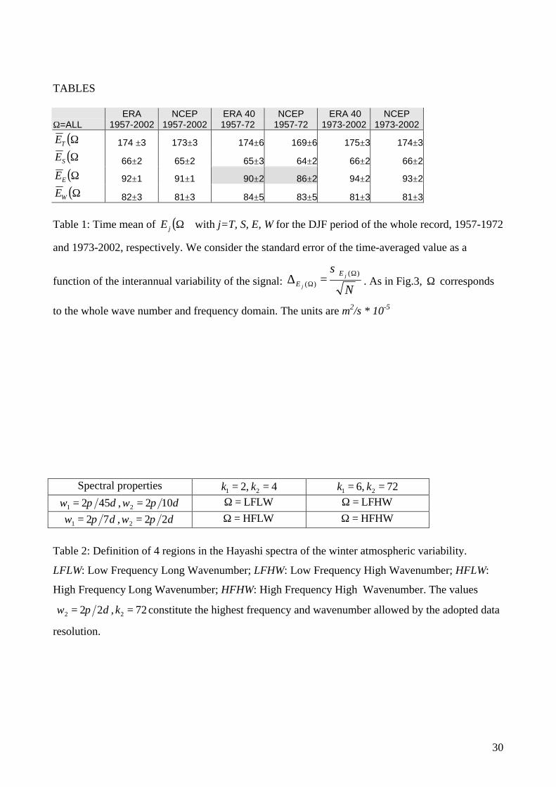
In table 1 we report the time average ( )ΩjE for the two reanalysis, computed over

the whole wave number and frequency domain. Total, standing, eastward, and

westward propagating energy spectrum are reported. Following basic statistical

arguments, we estimate the standard error of the time-averaged value as a function

of the interannual variability of the signal: Nj

j

EE

)()(

ΩΩ =∆

σ, where N is the number

of years considered in the averaging process. In the considered latitudinal band,

most of the energy is due to the eastward propagating component, as can be

inferred also from figure 1. In all cases the time-average of the ERA 40 signal is

10

larger, but the discrepancies between the averaged values for NCEP and ERA 40

don’t exceed the standard error )(Ω∆jE , with the exception of ( )ΩEE (gridded

cells in the table 1). This can be considered as an indication that NCEP and

ERA40 are significantly different in the description of eastward propagating

features.

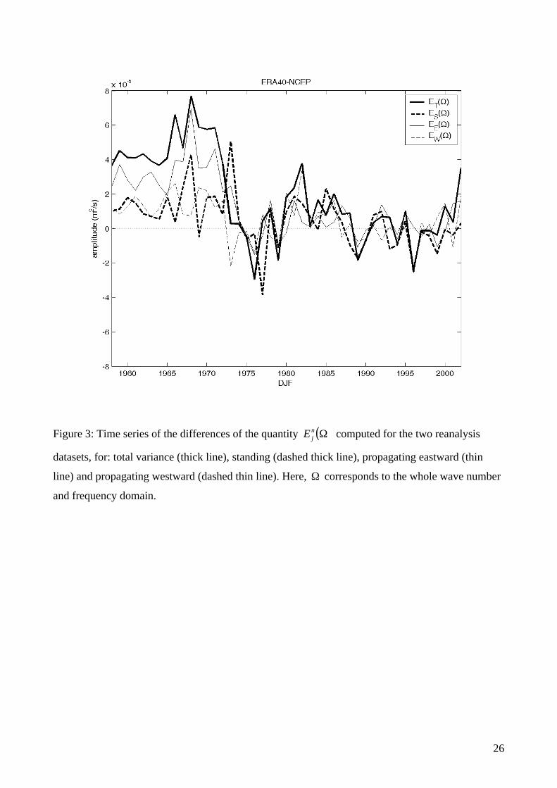
Inspection of the yearly differences in ( )ΩnjE for the total, standing and

eastward/westward propagating components (figure 3), reveal a systematic bias in

the period 1958-1972, with a major contribution from the eastward propagating

component. The mean difference in the following period is negligible.

For various choices of the spectral sub-domain Ω , the comparison of the

quantities ( )ΩnjE obtained from the two reanalyses can help identifying

differences in the capability of the two reanalyses in describing processes

occurring on a given spatial and temporal domain and pertaining to different

physical processes. In table 2 we propose a clear-cut division of the waves into

four categories, on the basis of the definition of Ω . The four categories are well-

separated and comprehend most of the wave energy of the atmosphere. As a

consequence of what shown in figures 1a-1d, we have that by computing ( )ΩjE

for the spectral sub-domains defined in table 2, we obtain that most of the energy

has to be attributed to the LFLW and HFHW waves. The absolute values of the

total energy content for each spectral subdomain are not reported. Instead, in

figure 4a-b we plot the corresponding difference time series for the sub-domains

LFLW and HFHW. The other sub-domains do not show significant differences.

We observe that the HFHW component (figure 4b) has a very large ratio between

the bias recorded in the first 15 years and the variability of the signal. The LFLW

term (figure 4a) also seems to have a bias in the first period, but of the same order

11

of magnitude of the overall interannual variability. The systematic differences

observed for the components HFHW and LFLW before 1973 correspond to

discrepancies of about 8% and 3% respectively, relative to the corresponding total

energy content.

12

4. Differences of the geopotential height fields

before and after 1973

In section 3 we have examined the discrepancies between the two reanalyses

emerging from a synthetic description of the activity of planetary and synoptic

waves. We now proceed by analysing the spatial distribution of the difference in

atmospheric variability reproduced by NCEP and ERA40 reanalysis.

In the previous section, a systematic bias was observed during the first 15 years of

the analysis. Therefore, we now divide the whole dataset into two periods, before

and after 1973. A preliminary comment is the concomitance of the date with the

use of the first meteorological information from satellites and aircraft data, both

assimilated in the reanalysis models (see

http://www.ecmwf.int/research/era/Data_Services/section3.html).

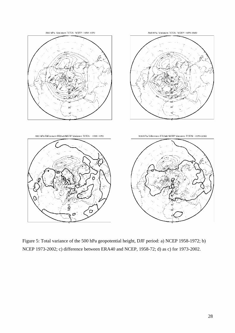
In figures 5a-d we plot the total variability for the NCEP data for the periods

1958-72 (Fig. 5a) and 1973-2002 (Fig. 5b), and the corresponding differences

with the same data for the ERA40 reanalysis (Figs. 5c-5d, respectively). The two

plots of the NCEP variance show that the atmospheric variability maximizes over

the oceanic basins (Blackmon, 1976). The main differences occur over these

regions for the whole period covered by the reanalyses, thus suggesting that the

representation of small scale features may be at the core of a systematic bias

between the two reanalyses. In the Atlantic sector the two reanalysis differ

strongly in the earlier period, while in the second period the accordance becomes

stricter. The relative differences in the total variability for the first period over the

Pacific and Atlantic regions are 10% and 3% respectively. We note also a

13

significant discrepancy over the Okhostsk Sea, where ERA40 has more variability

than NCEP (first period relative difference of the order of 10%).

The corresponding figure for the low frequency (LF) variability, obtained

discarding the frequency d102 πω > (see also table 2) in a Fourier transform of

the field, is not presented, showing the same features described for figure 5.

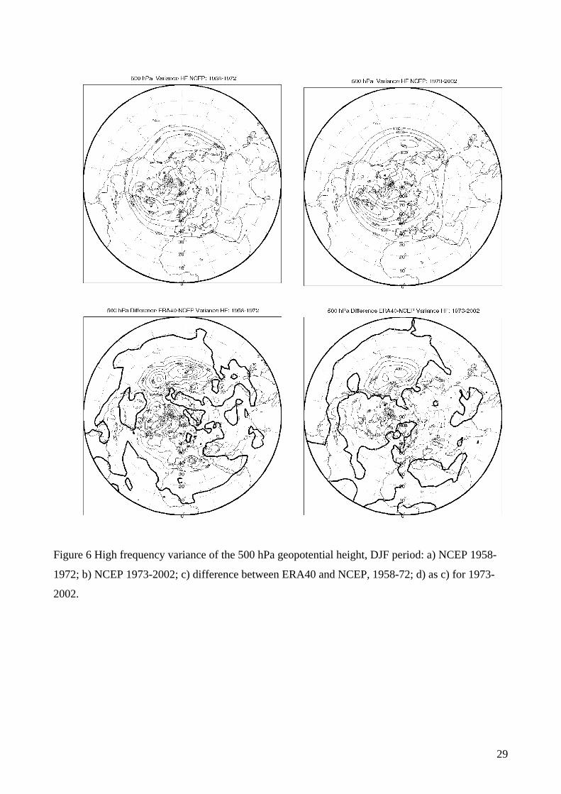
The spatial pattern of the high frequency (HF) variability ( dd 2272 πωπ ≤≤ , as

in table 2) is reported in figure 6. The NCEP HF variance shows a characteristic

feature of the synoptic disturbances, concentrated downstream of the jet maxima

in storm-track regions (Blackmon et al., 1977, Speranza, 1983, Wallace et al.,

1988). In the first period the ERA40 has more variability both over the Pacific and

the Atlantic sectors; the relative differences are of the order of 10%, with peaks of

about 20% over the Pacific on the central and exit area of the storm-track regions.

The difference pattern of the Atlantic sector entails the whole region between the

Hudson Bay and the Mediterranean basin. This latter difference disappears in the

second period, while the Pacific discrepancy reduces to a smaller area on the

eastern part of the basin. We emphasize that the discrepancies observed in the HF

component cannot be explained by a corresponding change in the jet stream where

the baroclinic waves grow (figure not shown).

14

5. Discussion and conclusions

The NCEP and ERA40 reanalyses have been compared for the overlapping period

1957-2002. Differences in the description of the northern hemispheric winters

have been quantitatively estimated by employing the space-time Fourier

decomposition introduced by Hayashi (1971, 1979). A few remarks should be

made about the limits of the methodology employed in this work. By computing

the cross-spectra and the coherence of the signal, the Hayashi decomposition

allows for the discrimination of the propagating and standing components of the

wavy patterns living on a given latitudinal circle or latitudinal belt. Therefore,

Hayashi spectra can capture only fundamentally one-dimensional features.

Instead, the two-dimensional dynamics of synoptic systems on the sphere have

considerable impact on the evolution of features that are tangent or that cross the

latitudinal belt considered for this work. The presence of such features leaves

spurious traces in the spectra considered in section 3. A second limit of Hayashi

spectra is that they necessarily describe features that have a periodic extension

over the whole latitudinal circle. Instead, important tropospheric features in the

high frequency subdomain, originate and decay at specific geographical location

(Tibaldi and Molteni, 1990). Nevertheless, Hayashi spectra have proved useful in

identifying some of the major biases between the two considered reanalyses.

We have focused on two main regions (HF and LF) of the total spectrum, where

reasonably well distinguishable processes are thought to affect the dynamics.

Our results show that, considering the HF and LF spectral features of the

atmosphere, disagreements between the two reanalyses can be found in the period

prior to 1973. In particular, the HF spectral component shows a sudden

improvement of the bias between the first and the second period. Instead, in the

15

low-frequency spectral region, it is more difficult to identify a similar transition.

In the high-frequency domain, the improvement is observe mainly over the

Atlantic basin, while in the Pacific basin differences in the variability described

by the two reanalyses remain approximately constant before and after 1973.

The coverage of the Northern Hemisphere by radiosondes, dominant over the land

regions, is relatively good and, to a large extent, uniform throughout the period

1958-1973 and further (Uppala et al., 2004). Therefore, the main discrepancies

between the two reanalysis in the early period should be due to other data source..

The analysis performed by Bengtsson et al. (2004) highlights the positive impact

of the radiosondes data over the land and of the satellite data over the ocean. Our

work confirms this behavior in the reanalysis and suggests also a relevant positive

impact of the aircraft data, introduced in the data assimilation process in 1973. In

fact the main improvement in the HF component of the Hayashi spectra can be

geographically located over the Atlantic Ocean (see figure 6), where the aircraft

data are mainly available. Besides, over the Pacific Ocean basin, where the

additional data are mainly from satellites, a weaker improvement is observed in

the atmospheric baroclinic waves description . These results suggest a caveat in

using the reanalysis data for the analysis of the low and high frequency variability

and trends prior to 1973. The investigation performed in this work provides us

some confidence level to use the reanalyses to validate the 500 hPa geopotential

height variability in climate models.

Thereby, our results agree with the findings of Hodges et al. (2003) and

Bengtsson et al. (2004) that when considering the analyzed fields prior to 1979

caution should be used because the analyses can be influenced by the model

deficiencies.

16

It remains to understand why the two models have different behaviors, both in the

HF and LF components , in the first period where data available are scarcer. The

possibility of verifying the actual relevance of our interpretation is out of our

reach since we can not re-run portions of the assimilation processes for both

reanalyses and check for consistency. However, we suggest some possible causes

of the observed discrepancies.

Dynamically, the simultaneous occurrence of significant discrepancies in both the

HF and LF spectral sub-domains may have two fundamentally different

interpretations. If the two spectral subdomains were dynamically independent,

then the two reanalysis procedures should differ both in the treatment of physical

processes which are responsible for LF variability and for processes related to the

development of synoptic disturbances. However, robust arguments about energy

cascades in geostrophic turbulence, suggest that energy can be transferred from

high to low-frequency. In this case, a difference observed in the standing

component could be attributed to the transfer of energy from smaller to larger

scale. (Savijarvi, 1978; Weeks et al., 1997). In support to the latter argument, we

found that a strong bias in the HFHW sub-domain exist in the first period and

corresponds to a noticeable bias in the LFLW.

After 1973, when the bias in the HFHW disappears, the bias in the LFLW also

disappears. However, the variability of the interannual discrepancies in the LFLW

sub-domain, remains larger than the initial bias itself, indicating that a mechanism

during all the reanalysis period acts to produce this error.

Such discrepancies in the description of basic physical processes may be

attributed most likely to one or both of the following characteristics of the models

used for the reanalyses.

17

The first is the resolution of the two models. The two models used for ERA40 and

NCEP reanalyses use spectral methods in the horizontal and finite difference

methods in the vertical. They mainly differ in the level of the truncation in the

horizontal (T63 for NCEP, T159 for ERA40) and in the number of vertical levels

(28 for NCEP, 60 for ERA40). The truncation level can influence the enstrophy

inverse cascade, and it can also affect the horizontal convergence of momentum,

which in turn alters the horizontal wind shear and controls the growth of the

baroclinically unstable eddies. Moreover, the vertical resolution should impact the

meridional and vertical heat fluxes associated to baroclinic perturbations that

modify the thermal vertical structure of the atmosphere in the midlatitudes (Barry

et al., 2000; Dell’Aquila, 2004).

Another aspect of the reanalyses ,which has been demonstrated to affect the low

frequency variability ,is the envelope orography, i.e. subgrid-scale orography

parameterization (Wallace et al., 1983; Tibaldi 1986). ERA40 uses an envelope

orography, whereas NCEP has a mean orography. For this parameterization the

smaller scales of the orography directly affect the zonal flow (Tibaldi, 1986).

This fact could explain the variability of the interannual discrepancies in the

LFLW sub-domain in the period after 1973.

18

Acknowledgments.

The authors wish to thank A. Sutera and A. Speranza for useful suggestions.

NCEP data have been provided by the NOAA-CIRES Climate Diagnostics

Center, Boulder, Colorado, from their web site at http://www.cdc.noaa.gov/. The

ECMWF ERA-40 data have been obtained from the ECMWF data server at

http://data.ecmwf.int/data/.

19

References

Annamalai H., Slingo J. M., Sperber K. R., Hodges K., 1999: The mean evolution and variability of the asian summer monsoon: comparison of ECMWF and NCEP-NCAR reanalyses. Mon. Wea. Rev., 127, 1157-1186.

Barry, L., Craig, G. C. and Thuburn, J. 2000. A GCM investigation into the nature

of baroclinic adjustment. J. Atmos. Sci. 57, 1141-1155. Bengtsson, L., K.I. Hodges, and S. Hagemann, 2004: Sensitivity of the ERA40

reanalysis to the observing system: determination of the global atmospheric circulation from reduced observations. Tellus, 56A, 456-471.

Benzi R., P. Malguzzi., A. Speranza and A. Sutera, 1986: The statistical properties

of general atmospheric circulation: observational evidence and a minimal theory of bimodality. Quart. J. Roy. Met. Soc., 112, 661-674.

Benzi, R. and Speranza, A., 1989: Statistical properties of low frequency

variability in the Northern Hemisphere. J. Climate 2, 367-379. Blackmon, M. L., 1976: A climatological spectral study of the 500 mb

geopotential height of the Northern Hemisphere. J. Atmos. Sci. 33, 1607-1623. Blackmon, ML, Wallace, JM, Lau, NC and Mullen, SL, 1977: An Observational

Study of the Northern Hemisphere Wintertime Circulation, J. Atmos. Sci., 34, 1040-1053.

Buzzi A., Trevisan A., and Speranza A., 1984: Instabilities of a baroclinic flow

related to topographic forcing, J. Atmos. Sci. 41, 637-650 Caires, S., Sterl, A., Bidlot, J.-R., Graham, A., and Swail, V., 2004:

Intercomparison of different wind wave reanalyses, J. Climate 17, 1893-1913. Charney, J. G., and Straus, D. M., 1980: Form-drag instability, multiple equilibria

and propagating planetary waves in the baroclinic, orographically forced, planetary wave system. J. Atmos. Sci. 37, 1157-1176

Dell’Aquila, A., 2004. Midlatitude winter tropopause: the observed state and a

theory of baroclinic adjustment. PhD Thesis, University of Genoa, Genoa. 100 pp.

Hayashi Y. 1979: A generalized method for resolving transient disturbances into

standing and travelling waves by space-time spectral analysis. J. Atmos. Sci., 36, 1017-1029.

Hansen, A. R., and A. Sutera, 1983: A comparison of the spectral energy and

enstrophy budgets of blocking versus non-blocking periods. Tellus, 36A, 52-63

20

Harrison M. J., Rosati A., Soden B. J., Galanti E., Tziperman E., 2002: An evaluation of Air-Sea Flux Products for ENSO Simulation and Prediction. Mon. Wea. Rev. 130, 723-732

Hodges K. I., Hoskins B. J., Boyle J., Thorncroft C., 2003: A comparison of

recent reanalysis datasets using objective feature tracking: storm tracks and tropical easterly waves, Mon. Wea. Rev. 131, 2012-2037.

Holton, J. R, 1992: An introduction to dynamic meteorology, Academic Press,

Boston, pp. 497 Josey S. A., 2001: A comparison of ECMWF, NCEP-NCAR, and SOC surface

heat fluxes with moored buoy measurements in the subduction region of the North Atlantic. J. Climate, 14, 1780-1789.

Josey S. A., Kent E. C., Taylor P. K., 2002: Wind stress forcing of the ocean in

the SOC climatology: comparison with the NCEP-NCAR, ECMWF, UWM/COADS, and Hellerman Rosenstein datasets. J. Phys. Oceangr., 32, 1993-2019

Kistler R, Kalnay E, Collins W, Saha S, White G, Woollen J, Chelliah M,

Ebisuzaki W, Kanamitsu M, Kousky V, van den Dool H, Jenne R, Fiorino M, 2001: The NCEP-NCAR 50-year reanalysis: Monthly means CD-ROM and documentation. Bull. Am. Meteorol. Soc. 82, 247–267

Pratt, R. W., 1976: The interpretation of space-time spectral quantities. J. Atmos.

Sci., 33, 1060–1066. Renfew I. A., Moore G. W. K., Guest P. S., Bumke K., 2002: A comparison of

surface layer and surface turbulent flux observation over the Labrador Sea with ECMWF Analyses and NCEP Reanalyses. J. Phys. Oceanogr., 32, 384-400.

Ruiz-Barradas, A., S. Nigam, 2004: Warm-season rainfall variability over the US

Great Plains in observations, NCEP and ERA-40 reanalyses, and NCAR and NASA atmospheric model simulations, J. Climate, in press

Savijarvi H., 1978: The interaction of the monthly mean flow and large-scale,

transient eddies in two different circulation types. Part II: vorticity and temperature balance. Geophysica 14, 207-229.

Simmons, A. J. and J. K. Gibson, 2000: The ERA-40 Project Plan, ERA-40

Project Report Series No. 1, ECMWF, 62 pp. Speranza, A., 1983: Determinist and statistical properties of the westerlies.

Paleogeophysics 121, 511-562 Sturaro, G., 2003: A closer look at the climatological discontinuities present in the

NCEP/NCAR reanalysis temperature due to the introduction of satellite data. Climate Dyn., 21, doi:10.1007/s00382-003-0348-y.

21

Tibaldi, S., 1986: Envelope orography and maintenance of the quasi-stationary circulation in the ecmwf global models., Advances in Geophysics. Vol. 29 Academic Press 227-249.

Tibaldi, S. and F. Molteni, 1990: On the operational predictability of blocking.

Tellus, 42A, 343-365 Sakari Uppala, Per Kållberg, Angeles Hernandez, Sami Saarinen, Mike Fiorino,

Xu Li, Kazutoshi Onogi, Niko Sokka, Ulf Andrae and Vanda Da Costa Bechtold ERA-40: ECMWF 45-year reanalysis of the global atmosphere and surface conditions 1957–2002. ECMWF Newsletter No. 101 – Summer/Autumn 2004

Wallace, J.M., Tibaldi, S., and A. Simmons, 1983: Reduction of systematic

forecast-error in the ECMWF model through the introduction of an envelope orography. Q.J.R. Meteorol. Soc., 109, 683-717.

Wallace, J. M., G.-H. Lim, and M. L. Blackmon. 1988. Relationship between

cyclone tracks, anticyclone tracks and baroclinic waveguides. J. Atmos. Sci. 45, 439-462.

Weeks ER, Tian Y, Urbach J. S., Ide K., Swinney H. L., and Ghil M., 1997:

Transitions Between Blocked and Zonal Flows in a Rotating Annulus with Topography, Science 278, 1598-1601

22

Appendix: Space-time spectral analysis

The space-time spectral analysis, introduced by Hayashi (1971), provides

information about the direction or speed at which the eddies move.

This information may be obtained by, firstly, Fourier-analysing the spatial field

and then computing the time-power spectrum of each spatial Fourier component.

The difficulty here lies in the fact that straightforward space-time decomposition

will not distinguish between standing and traveling waves: a standing wave will

give two spectral peaks corresponding to traveling waves moving eastward and

westward at the same speed and the same phase. The problem can only be

circumvented by making assumptions regarding the nature of the wave. For

instance, we may assume complete coherence between the eastward and westward

components of standing waves and attribute the incoherent part of the spectrum to

real traveling waves (Pratt, 1976, Fraedrich and Bottger, 1978; Hayashi,1979).

In this formulation, for each winter considered, the energy spectrum ( )ω,/ kH WE

at a zonal wavenumber k and temporal frequency ω for the eastward and

westward propagating waves is :

(A1a) ( ) ),()()(, 21

41

kkkkE SCQSPCPkH ωωωω ++=

(A1b) ( ) ),()()(, 21

41

kkkkW SCQSPCPkH ωωωω −+=

Pω and Qω are, respectively the power and the quadrature spectrum of the

longitude (λ) and the time (t) dependent 500hPa geopotential height ( )tZ ,λ

expressed in terms of the zonal Fourier harmonics:

(A2) ( ) ( ) ∑∞

++=1

0 .)sin()()cos()(,, λλλλ ktSktCtZtZ kk

23

The total variance spectrum ( )ω,kHT is given from the sum of the eastward and

westward propagating components:

(A3) ( ) ( ))()(, 21

kkT SPCPkH ωωω +=

while the propagating variance ( )ω,kHP is given by the difference between the

components (A1a) and (A1b):

(A4) ( ) ( ).,, ωω kQkHP =

So, the standing variance spectrum ( )ω,kHS can be obtained by the difference:

(A5) ( ) ( ) ( )ωωω ,,, kQkHkH TS −= .

We emphasize that for sake of simplicity of the notation we have neglected the

indication of the winter under investigation, denoted in the text by the superscript

n.

We emphasize that customarily, Hayashi spectra are generally represented by

plotting the quantities ( )ωπω ,2 kHk T⋅⋅ , ( )ωπω ,2 kHk S⋅⋅ , ( )ωπω ,2 kHk E⋅⋅ ,

and ( )ωπω ,2 kHk W⋅⋅ , as reported in figures 1a-1d, in order to allow for equal

geometrical areas in the log-log plot representing equal variance.

24

Figure 1: Climatological average over 45 winters of Hayashi spectra for 500 hPa geopotential

height (relative to the latitudinal belt 30°N-75°N) from NCEP data: ( )ω,kHT (a); ( )ω,kH S (b);

( )ω,kHE (c); ( )ω,kHE (d). The Hayashi spectra have been obtained multiplying the energy spectra

by πω 2⋅k . The units are m2/s * 10-5

25

Figure 2: As for figure 1 but for the difference between ERA40 and NCEP dataset Hayashi spectra.

Dashed lines are pertaining to negative values.

26

Figure 3: Time series of the differences of the quantity ( )ΩnjE computed for the two reanalysis

datasets, for: total variance (thick line), standing (dashed thick line), propagating eastward (thin

line) and propagating westward (dashed thin line). Here, Ω corresponds to the whole wave number

and frequency domain.

27

Figure 4: As in figure 3 for the categories LFLW (a), HFHW (b) described in table 2.

28

Errore.

Figure 5: Total variance of the 500 hPa geopotential height, DJF period: a) NCEP 1958-1972; b)

NCEP 1973-2002; c) difference between ERA40 and NCEP, 1958-72; d) as c) for 1973-2002.

29

Figure 6 High frequency variance of the 500 hPa geopotential height, DJF period: a) NCEP 1958-

1972; b) NCEP 1973-2002; c) difference between ERA40 and NCEP, 1958-72; d) as c) for 1973-

2002.

30

TABLES

Ω=ALL ERA

1957-2002 NCEP

1957-2002 ERA 40 1957-72

NCEP 1957-72

ERA 40 1973-2002

NCEP 1973-2002

( )ΩTE 174 ±3 173±3 174±6 169±6 175±3 174±3

( )ΩSE 66±2 65±2 65±3 64±2 66±2 66±2

( )ΩEE 92±1 91±1 90±2 86±2 94±2 93±2

( )ΩWE 82±3 81±3 84±5 83±5 81±3 81±3 Table 1: Time mean of ( )ΩjE with j=T, S, E, W for the DJF period of the whole record, 1957-1972

and 1973-2002, respectively. We consider the standard error of the time-averaged value as a

function of the interannual variability of the signal: Nj

j

EE

)()(

ΩΩ =∆

σ. As in Fig.3, Ω corresponds

to the whole wave number and frequency domain. The units are m2/s * 10-5

Spectral properties 4 ,2 21 == kk 72 ,6 21 == kk dd 102 ,452 21 πωπω == LFLW=Ω LFHW=Ω

dd 22 ,72 21 πωπω == HFLW=Ω HFHW=Ω

Table 2: Definition of 4 regions in the Hayashi spectra of the winter atmospheric variability.

LFLW: Low Frequency Long Wavenumber; LFHW: Low Frequency High Wavenumber; HFLW:

High Frequency Long Wavenumber; HFHW: High Frequency High Wavenumber. The values

72,22 22 == kdπω constitute the highest frequency and wavenumber allowed by the adopted data

resolution.