1

AEROSOLS FOR CONCENTRATING SOLAR ELECTRICITY

PRODUCTION FORECASTS: REQUIREMENT QUANTIFICATION AND

ECMWF/MACC AEROSOL FORECAST ASSESSMENT

Dr. Marion Schroedter-Homscheidt, German Aerospace Center (DLR), Earth Observation

Center, 82234 Oberpfaffenhofen, Germany, phone +49 8153 282896, email marion.schroedter-

homscheidt@dlr.de (corresponding author)

Dr. Armel Oumbe, Total Gas & Power, R&D – Concentrated Solar Technologies, France;

former affiliation: Deutsches Zentrum für Luft- und Raumfahrt (DLR), Earth Observation

Center, Oberpfaffenhofen, Wessling, Germany

Dr. Angela Benedetti, Dr. Jean-Jacques Morcrette, European Centre for Medium-Range Weather

Forecasts (ECMWF), Data Assimilation Section, Reading, UK

ManuscriptClick here to download Manuscript: schroedter_homscheidt_aerosol_user_requirements_final_after_review.docx

2

ABSTRACT

The potential for transferring a larger share of our energy supply towards renewable is a widely

discussed goal in society, economics, environment and climate-related programs. For a larger

share of electricity to come from fluctuating solar and wind energy-based electricity, production

forecasts are required to ensure successful grid integration. Concentrating solar power holds the

potential to make the fluctuating solar electricity a dispatchable resource by using both heat

storage systems and solar production forecasts based on a reliable weather prediction. These

solar technologies exploit the direct irradiance at the surface, which is a quantity very dependent

on the aerosol extinction with values up to 100%. Results from present-day numerical weather

forecasts are inadequate, as they generally use climatologies for dealing with aerosol extinction.

Therefore, meteorological forecasts have to be extended by chemical weather forecasts. The

paper aims at quantifying on a global scale the question if and where daily mean or hourly

forecasts are required, or if persistence is sufficient in some regions. It assesses the performance

of recently introduced NWP aerosol schemes by using the ECMWF-MACC forecast which is a

preparatory activity for the upcoming European GMES (Global Monitoring for Environment and

Security) Atmosphere Service.

3

CAPSULE

Helping to stabilize the electricity grid facing larger solar energy shares: Integration of aerosol

forecasts into existing numerical weather prediction schemes

4

USER REQUIREMENTS FROM THE SOLAR SECTOR 1

Concentrating Solar Power (CSP) systems use lenses or mirrors and tracking systems to focus a 2

large area of sunlight onto a small area. A working fluid is heated by the concentrated sunlight, 3

and this thermal energy can be stored or immediately used to produce electricity via a steam 4

turbine. Alternatively, concentrating photovoltaics (CPV) are a future technology with growing 5

interest among industries, where sunlight is concentrated on smaller and highly efficient, but 6

rather expensive photovoltaic cells. Concentrating technologies utilize direct normal irradiance 7

(DNI) which is the direct irradiance on the normal plane with respect to the incoming beam. 8

Typically, DNI is measured as the incoming irradiance from the sun‟s disc together with 9

circumsolar diffuse irradiance within a cone of 2.5° around the sun center (WMO, 2008). 10

Sunlight is the fuel for each solar energy conversion system. Like any generation source, 11

knowledge about the fuel‟s quality and future reliability is essential for an accurate estimate of 12

technical system performance and financial viability of a project. For site selection, choosing the 13

optimum energy conversion technology, or designing systems for specific locations, it is 14

necessary to understand the long-term spatial and temporal variability of available solar 15

resources. For these applications long-term annual or monthly irradiation sums together with 16

accurate frequency distributions of solar irradiance are needed and provided with the help of 17

satellite data (Cano et al., 1986; Beyer et al., 1996; Rigollier et al., 2004). However, short- and 18

medium-term forecasts of the solar resource will remain essential to the plant‟s efficient 19

operations and its integration into the electricity grid throughout its lifetime. 20

It has to be noted, that users from the non-concentrating photovoltaic technology sector require a 21

high global irradiance forecast accuracy. This can mainly be achieved through high cloud 22

5

forecast accuracy, while aerosols are of only minor importance for this purpose. On the other 23

hand, users from the CSP sector need a high DNI forecast accuracy especially in cloud-free cases 24

with high DNI. Additionally, CSP users request a good forecast on the occurrence of low DNI 25

cases - which refers mainly to a good water cloud mask forecast - and a good forecast of medium 26

DNI cases – which refers to the cirrus cloud optical properties forecast. CSP technologies 27

generally operate only in areas with high DNI and small cloud cover. Therefore, depending on 28

the geographical region of interest and its vicinity to global aerosol sources, the priority is set 29

either on good aerosol or cirrus forecasts. This paper focuses on the aerosol forecast accuracy, 30

while assessing the requirements on cirrus clouds and the modeling capabilities in today‟s NWP 31

would be a separate subject. 32

CSP electrical energy production can be calculated by using a power plant model and DNI as an 33

input parameter. The power plant model has to simulate the thermal state of the heat transfer 34

fluid and its pumping through the solar field; the hot and cold heat storage tank‟s status; heat 35

exchangers used between the solar field, tanks and the turbine; technical turbine specifics, and 36

finally, a model of the manual and interactive control of the power plant by its operator team 37

(e.g. Wittmann et al., 2008; Klein et al., 2010; Wagner et al., 2011). 38

The strong dependency between DNI and CSP electricity production makes forecasting of direct 39

solar irradiance essential (Pulvermüller et al., 2009; Wittmann et al., 2008). In the Spanish 40

electricity market for example, the hourly electrical energy production forecast for a given day 41

has to be delivered on the previous day before 10 AM (Real Decreto 661/2007). A high quality 42

forecasting system reduces the power plant operator‟s risk of penalty payments due to inaccurate 43

production forecasts and helps the transmission grid operator to keep operations stable. 44

According to the Spanish regulation, penalties apply to cover additional costs occurring for the 45

6

electricity grid operator in case of inaccurate electricity production forecasts provided by the 46

power plant operator. E.g. in case of a lower production than predicted in a certain hour of the 47

day, the electricity grid operator might need to purchase additional electricity from other sources 48

on the short-term electricity market. These extra costs can be forwarded to the power plant 49

operator as a penalty. Penalties may apply if production forecasts are too small – resulting in 50

additional purchase needs – or too high – resulting in additional selling needs at the grid 51

operator‟s side. Penalties apply only if costs occurred in reality – e.g. a lower production than 52

predicted which occurs in a situation with lower electricity consumption than predicted might not 53

cause any additional purchase needs and therefore no costs. 54

Kraas et al. (2010 and 2011) analyzed how a good DNI forecast can enhance the profitability of 55

a power plant when operating at a day-ahead electricity market. In their case study for a power 56

plant in Southern Spain, a relative DNI forecasting error magnitude of 10-20% and 20-30% 57

respectively lead to 1.5 euro/MWh and 2.5 euro/MWh penalties in a reference year based on 58

actual market conditions. A 10% improvement in forecasting leads to a penalty reduction of 59

about 7%. Additionally, an accurate production forecast can increase plant profits by optimizing 60

energy dispatch into the time periods of greatest value on the electricity markets. 61

The current state of the art in NWP provides rather inaccurate DNI forecasts. Lara-Fanego et al. 62

(2012) found a relative RMSE of 60% for hourly DNI forecasts in Spain using a WRF-ARW 63

(version 3) model implementation for all sky conditions (cloudy as well as cloud-free). In 64

overcast skies, knowledge of cloud cover and type is most important. Nevertheless, in high solar 65

resource regions as the Mediterranean and Northern Africa, because less cloudy, aerosol loading 66

is the most critical atmospheric parameter since up to 30% of additional direct irradiance 67

extinction have been reported (e.g. Gueymard, 2003 and 2005; Wittmann et al., 2008). In dust 68

7

outbreak events, the extinction of DNI reaches even up to 100%. Breitkreuz et al. (2009) 69

compared direct irradiances calculated from AERONET measurements, the ECMWF operational 70

model and EURAD (Forecasted AOD of the European Dispersion and Deposition Model) based 71

AOD forecasts in order to quantify the effects of varying AOD forecast quality on solar energy 72

applications. They show that a chemical transport model designed for air quality research is 73

strongly needed for solar irradiance forecasting in clear sky conditions. It improves the relative 74

RMSE from 31% to 19% in clear sky conditions. 75

As part of the MACC project (Monitoring Atmospheric Composition and Climate) within the 76

European Union's Global Monitoring of Environment and Security (GMES) program, the 77

European Centre for Medium Range Weather Forecasts (ECMWF) Integrated Forecast System 78

(IFS) has recently been modified to include a chemical weather prediction suite, which provides 79

an analysis and subsequent forecast of aerosols (Benedetti et al., 2009; Morcrette et al., 2009, 80

2011). This opens the field for improved NWP-based DNI forecasts by using an operational 81

aerosol forecast. 82

The objectives of this paper are to quantify which accuracy and temporal resolution are needed 83

on aerosol optical depth (AOD) forecasts with respect to hourly DNI forecasts. This includes the 84

questions whether and where a daily mean forecast or a two-day persistence approach might be 85

sufficient. Finally, MACC AOD forecasts are assessed and compared versus the 2-day 86

persistence approach in order to give a first impression whether the recently introduced aerosol 87

modeling in NWP centers is already applicable for the solar user community. 88

AERONET AOD MEASUREMENTS USED 89

8

Ground-based sun photometer measurements made in the AERONET (AErosol RObotic 90

NETwork) network are used as reference for each forecast validation and for estimating the 91

intra-day AOD variation at 550 nm. The accuracy of AOD values is ±0.01 for wavelengths larger 92

than 440 nm (Holben et al., 1998). In this study, all 537 Level 2.0 (cloud-screened and quality-93

assured) AERONET stations operating during any phase inside the period August 1992 to 94

January 2011 are used. The exact period of measurements changes from few months 95

corresponding to a particular campaign to years for each station. All AERONET measurements 96

within an hour are used to create hourly mean values. A station is considered only if there are at 97

least 100 matching hours. The availability of only clear-sky and daytime observations is well 98

suited to assess a parameter relevant for concentrating solar energy applications, as they operate 99

mainly in the same conditions. 100

ECMWF/MACC AEROSOL FORECAST 101

The Global and regional Earth-system Monitoring using Satellite and in situ data (GEMS) 102

project developed the capability of modeling atmospheric constituents such as aerosols, 103

greenhouse and reactive gases within the European Centre for Middle-Range Weather 104

Forecasting (ECMWF). This prognostic aerosol scheme has been used in the ECMWF Integrated 105

Forecast System (IFS) in both its analysis and forecast modules to provide a re-analysis and a 106

near-real-time (NRT) run. Five types of tropospheric aerosols are considered: sea salt, dust, 107

organic and black carbon, and sulfate. The two natural aerosols sea salt and dust have their 108

sources linked to prognostic and diagnostic surface and near-surface model variables. In contrast, 109

organic matter, black carbon and sulfate have their external source databases. Physical processes 110

as dry deposition including the turbulent transfer and gravitational settling to the surface and wet 111

9

deposition including rainout and washout of aerosol particles in and below the clouds are 112

considered. MODIS observations of AOD at 550 nm from collection 5 and 6 (Remer et al., 2005) 113

from both the Terra and Aqua satellites are assimilated in the ECMWF operational four-114

dimensional assimilation system (Rabier et al., 2000; Mahfouf et al., 2000; Klinker et al. 2000). 115

A more detailed description of the MACC NRT run is found in the Morcrette et al. (2009 and 116

2011) and Benedetti et al. (2009). ECMWF/MACC AOD 550 nm forecasts in three-hourly 117

resolution with forecast duration of 48 hours were obtained on a reduced N80 Gaussian grid with 118

a resolution of 1.125° in latitudes. At the time of this study ECMWF/MACC data had been 119

available for the period September 2009 to December 2010. Since measurements at some 120

AERONET stations originate from a short-term campaign and due to the delay in the availability 121

of quality controlled Level 2.0 data, there are fewer stations available for ECMWF/MACC 122

validations than for pure AERONET based assessments. 123

ASSESSMENT METHOD 124

The classical approach of comparing measured and forecasted AOD time-series would be to 125

investigate differences in AOD (ΔAOD, marked with a red symbol in Fig. 1). In this study, we 126

are interested in errors in DNI caused by a ΔAOD at an individual hour of the day – Fig 1 127

illustrates the assessment method used. A ΔAOD generates a different ΔDNI for high and low 128

aerosol loadings, and ΔDNI also depends on the solar zenith angle and the aerosol type (Fig. 2, 129

details explained below). Therefore, hours with a ΔAOD being greater than a critical AOD 130

difference (ΔAODcrit) are counted. Values ΔAODcrit are defined as the threshold when a more 131

than x% DNI deviation is caused by the actual ΔAOD with respect to solar position and the AOD 132

value itself. This results in the user-specific exceedance hour parameter which corresponds to the 133

10

percentage of hours when an AOD deviation leads to at least a 5, 10 or 20% DNI deviation. Such 134

a probability of exceedance can be used in economic assessments more easily than any ΔAOD 135

information. Additionally, ΔDNI is derived from ΔAOD generating standard parameters as the 136

relative bias and the relative root mean square deviation (RMS). 137

The solar sector does not provide a single number of an acceptable maximum hourly DNI 138

deviation as the acceptable DNI forecast accuracy is dependent on the economic viability of a 139

power plant. This depends on many, partly time-varying factors like the electricity market prices, 140

loan conditions for investors, regulation requirements from national authorities, the potential 141

return-on-investment for alternative investments, and last but not least on the concentrating solar 142

technology chosen among a variety of technology options. Therefore, this paper provides results 143

for different ΔDNI ranges and assumes that a power plant developer will use the results being 144

appropriate for a specific solar power plant project development. 145

For the derivation of ΔAODcrit thresholds and for all solar surface irradiance calculations, the 146

radiative transfer model libRadtran (library for Radiative transfer; Mayer and Kylling, 2005) 147

with its solver DISORT (Stamnes et al., 1988) is used. Its accuracy has e.g. been demonstrated in 148

Kylling et al. (2005). Since CSP systems use the complete solar spectrum, only the broadband 149

direct irradiance is of interest and transferred towards DNI by using the cosine of the sun zenith 150

angle (SZA). Values of ΔAODcrit are estimated (Fig. 2) for various aerosol optical depths (AOD), 151

for the four OPAC (Optical Properties of Aerosols and Clouds; Hess et al., 1998) aerosol types 152

used, and varying SZA. By requiring a minimal 10 W/m2 ΔDNI, very small DNI values are 153

excluded. The generation of this database acts as a pre-requisite to derive the paper‟s statistical 154

results in the next chapters. Generally, ΔAODcrit is increasing with the AOD, while for small 155

AOD, ΔAODcrit is decreasing with larger SZA reflecting the larger air mass. On the other hand 156

11

for high AOD, ΔAODcrit strongly increases with SZA due to the anyhow large extinction of 157

irradiance. As the surface irradiance at such AOD values gets small, the required minimum 158

deviation of 10 W/m2 is more difficult to reach resulting in this increase of the threshold with 159

SZA. 160

It has to be noted that the DISORT solver treats the sun as a point source and therefore neglects 161

circumsolar radiation as seen by a pyrheliometer with a typical half-field of view of 2.5°. 162

Therefore, DNI in this study is not exactly the DNI value as measured with standard 163

pyrheliometers. Generally, this effect is small in the aerosol case, while it becomes a up to 50% 164

effect on the transmittance in the case of cirrus clouds (e.g. Shiobara and Asano, 1994; Thomalla 165

et al., 1983). This cirrus effect is neglected assuming that the AERONET level 2 observations are 166

successfully cloud-corrected. 167

Both AERONET and ECMWF/MACC forecasts provide spectral AOD describing the aerosol 168

type implicitly. In LibRadtran calculations, pre-set aerosol types based on OPAC are used. This 169

assumption is certainly not true for each individual hour, but simplifies the approach. 170

Additionally, this study is performed for CSP technologies exploiting broadband direct 171

irradiances and therefore, being not as sensitive to the aerosol type as e.g. future thin film 172

photovoltaic technologies. Therefore, also details of the ECMWF/MACC aerosol type 173

characterization resulting in spectral AOD errors are outside the focus of this study. The OPAC 174

aerosol type “continental average” is used at most stations. Cities with more than 2 million 175

inhabitants are marked as urban (29 stations). Stations listed by Huneeus et al. (2010) as dusty 176

are considered as having a desert aerosol type (23 stations). Finally, a visual selection of 177

maritime aerosol type for stations close to the sea or on small isolated islands is made (26 178

12

stations). Lists of aerosol urban type, desert type and maritime type stations are given in 179

appendix A. 180

In this paper we concentrate on requirements for aerosol forecasts. Therefore, all comparisons 181

assume that DNI is only sensitive to aerosol loading. Aerosol loading is the most significant 182

input parameter in clear skies, but depending on SZA and aerosol loading itself, the influence of 183

other atmospheric parameters can be more or less important. A sensitivity study based on 184

randomly selected 50 variations of aerosol Angstrom exponent, total column water vapor, total 185

column ozone, altitude of the ground, ground albedo and atmospheric profile is made. For each 186

tuple of AOD, aerosol type, and SZA used in Fig. 2, the relative RMS in computed (Fig. 3, left). 187

The influence of other parameters changes with the amount of AOD. This deviation can be very 188

large in highly turbid conditions reaching even extreme values higher than 50%. This occurs 189

only in conditions with DNI less than 200 W/m2 (Fig. 3, right) which are not relevant for 190

concentrating solar technologies. 191

IS A DAILY MEAN FORECAST SUFFICIENT? 192

It has been discussed whether the use of a daily AOD forecasts is sufficient for a DNI forecast in 193

some regions of the world. Therefore, the ΔDNI due to intra-day AOD variation is quantified at 194

the location of each AERONET station (Fig. 4) by comparing AERONET-derived daily AOD 195

means versus hourly means in each forecast hour. In general, the intra-day variation of AOD 196

leads to a small ΔDNI. In most stations, the percentage of hours with a ΔAOD leading to more 197

than 20% ΔDNI is less than 10%. For the stricter criterion of a more than 5% ΔDNI, around 30% 198

of exceedance hours are found in the EUMENA (Europe, Mediterranean and Northern Africa) 199

13

region and Northern America and 60% in South East Asia. The mean relative bias and RMS in 200

DNI are rather low having values generally less than 10%. 201

A daily cycle with higher ΔDNI at low solar elevations and smaller values in the middle of the 202

day is found. Therefore, the influence of the AOD intra-day variation on DNI is less important 203

when there is more solar resource available during noon hours. Additionally, deviations are 204

generally higher for urban and desert aerosol type dominated stations having a larger variability 205

in AOD. 206

PERFORMANCE OF A TWO-DAY PERSISTENCE FORECAST AS 207

POOR MAN‟S APPROACH 208

Typically, it is required in an electricity production system to deliver the day ahead energy 209

production forecast of a power plant during morning hours e.g. before 10 AM in the Spanish 210

case. Therefore, a two-day persistence - defined as AOD(t+48) being equal to AOD(t) for each 211

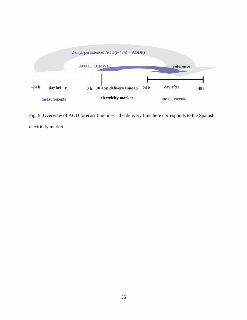
hourly mean AERONET value (Fig. 5) - is assessed instead of a standard one-day persistence. 212

The persistence acts both as a potential poor man‟s approach as well as a reference case for each 213

other forecasting approach (next section). 214

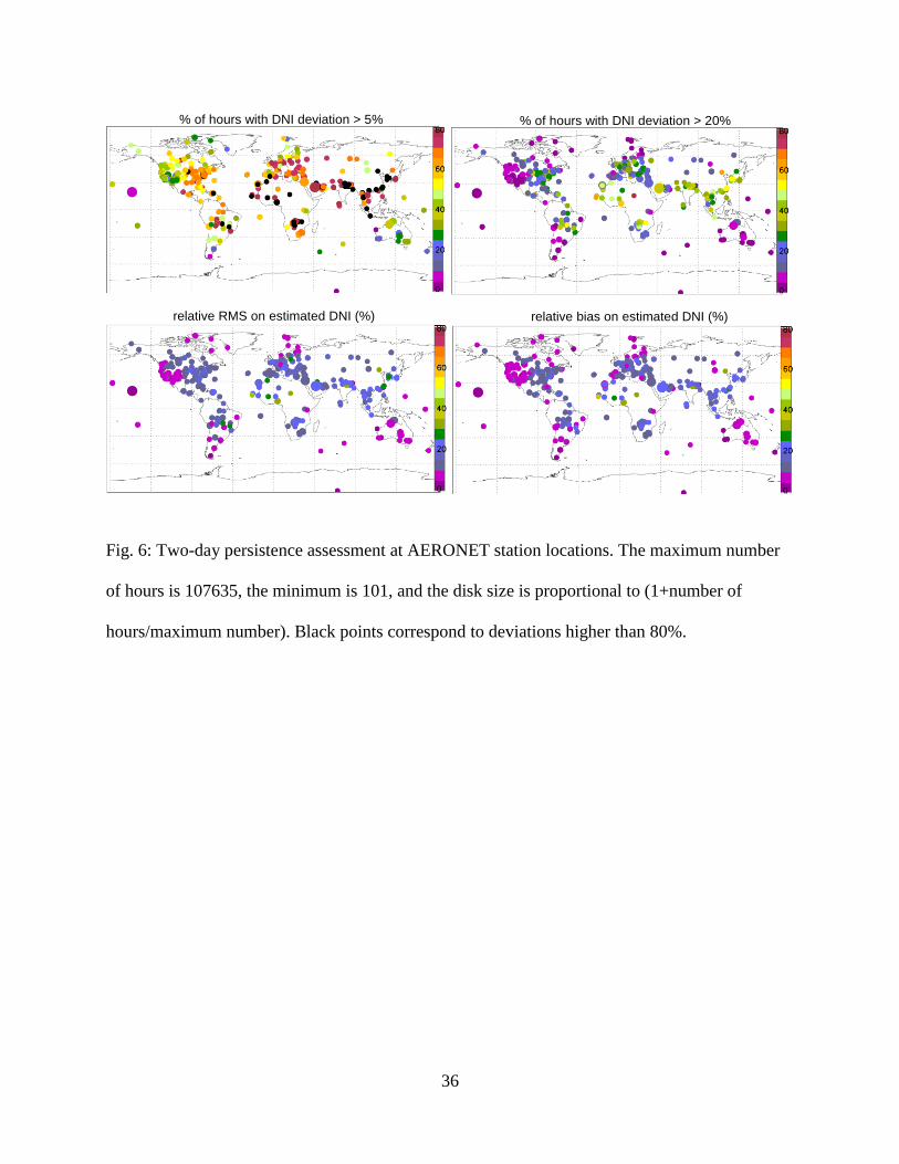
The relative ΔDNI tends to increase with the mean AOD: Large exeedance hour values are 215

obtained in the Middle-East and South-East Asia for the 20% criterion, while a large number of 216

exceedance hours is also recorded in African areas close to source areas (Fig. 6). Minima are 217

obtained in Australia and Northern America (around 10%) and maxima in South-East Asia and 218

south of the Sahara (around 70%). A similar result is found for exeedance hours due to a two-day 219

persistence for the 5% DNI deviation threshold, with an obviously higher percentage of 220

14

exceeding cases: 70% for EUMENA and the East of Northern America and 90% for South-East 221

Asia and regions close to African deserts. Generally, a two-day persistence of hourly AOD is not 222

accurate enough for DNI forecasting at all stations in the EUMENA region, but might be 223

sufficient in Australia, the Western US, and parts of Southern America depending on the critical 224

deviation threshold chosen by the user based on technical and economic considerations. 225

Deviations are at least two times lower from 10h to 15h true solar time (TST) than in other 226

periods of the day for most stations. Additionally, for continental average and maritime clean 227

types, there is only around 10% of hours with an AOD deviation leading to at least a 20% DNI 228

deviation during the most energetic period of the day. 229

PERFORMANCE OF A GLOBAL STATE OF THE ART NWP 230

AEROSOL MODEL 231

Using the scheme described in Fig. 1 the ECMWF/MACC AOD forecasts out of the 0 UTC run 232

for day 2 (25 to 48 h lead time) are validated against AERONET measurements (Fig. 7). It has to 233

be noted that there are spatio-temporal errors due to the comparison of the model grid average 234

versus a point measurement. On the other hand, this is exactly the user‟s approach when 235

applying a global NWP model to forecast DNI for solar power plant sites of a maximum size of 236

1-2 km². From the user‟s point of view there might be a discrepancy between a local 237

measurement and the model forecast – whether this is related to any model error or unresolved 238

sub-grid scale variability is not relevant for users. Therefore, this validation approach is 239

consistent with the potential use of such forecasts. 240

15

Rather low relative DNI RMS and bias are obtained: generally, values between 5 and 15% are 241

found, although higher deviations are observed in South-East Asia and at the west coast of 242

Africa. The percentage of hours with a ΔDNI larger than 20% is also low, especially in the 243

western US, where it is less than 10%. This percentage remains generally less than 20% in the 244

Eastern US, in Europe as well as in Southern America and Australia. Remarkably higher 245

percentages are obtained for all stations if the critical ΔDNI is set to 5%. Some stations - in black 246

- even exhibit percentages higher than 80%. 247

The error measures as a function of true solar time have similar shapes as those observed for the 248

two-day persistence. The percentage of hours is highly hourly sensitive, but being less in hours 249

with larger DNI. Values around 10% are found between 10 h and 14 h TST and reach 25% at 6 250

or 18 h TST for the 20% criterion. For the 5% criterion they are around 45% between 10 h and 251

14 h TST and reach 75% at 6 or 18 h TST. 252

Error measures of the ECMWF/MACC forecast are also compared to that of the two-day 253

persistence approach (Fig. 8). Positive difference of the individual error measures correspond to 254

stations where ECMWF/MACC performs better, while negative values represent AERONET 255

stations when the two-day persistence is advantageous. ECMWF/MACC performs better at most 256

stations, especially in Europe. The performance in the Western US is generally very good (Fig. 257

7), therefore, it is not significant that the two-day persistence performs better there. In Eastern 258

Asia, as well as in Western Africa, the ECMWF/MACC forecast is not fully able to describe the 259

regional features leading to statistical measures worse than the two-day persistence. That might 260

be due to a rapid Asian industrialization which is not yet taken into account in most emission 261

databases and to a yet incomplete knowledge of dust mobilization and transport. 262

16

CONCLUSIONS 263

An assessment of requirements on aerosol forecasting capabilities with special respect to solar 264

energy usage has been made. Critical thresholds of AOD deviation are generated and used in 265

statistics of exceedance hours, when the AOD deviation is relevant with respect to a certain 266

maximum DNI deviation accepted. This measure takes into account that the relative deviation on 267

the solar energy received at the power plant is a non-trivial function of ΔAOD being reflected in 268

radiative transfer theory. The same ΔAOD value in a specific hour of the day can be of relevance 269

or not depending on the solar position and the actual AOD itself. This complex dependency is 270

the explanation why existing, classical AOD forecast verification against AERONET as e.g. in 271

Morcrette et al. (2011) is indeed meaningful, but not sufficient for solar energy applications. 272

In the paper results for 5 and 20% DNI deviations are shown while the study was also performed 273

for a 10% deviation. Nevertheless, it is expected that each user group will define their own 274

acceptable DNI deviation, as this depends very much on specific design parameters of the chosen 275

solar technology and actual economic conditions assumed in viability assessments of a specific 276

power plant. Therefore, this paper presents both a harsh and a loose criterion as a first orientation 277

for the user community and as a justification of the design of future aerosol forecasting 278

capabilities at the meteorological centers. 279

With exception of South-East Asia, the influence of the AOD daily variation on hourly DNI 280

deviations is small if the 20% DNI deviation criterion is assessed. This assumption cannot be 281

made in most regions if a stricter DNI deviation criterion is applied. Additionally, lower DNI 282

deviations are found during small solar zenith angles around noon in the most energetic phase of 283

the day. Areas like Australia, the Western US, oceanic regions and southern parts of South 284

17

America can be treated with the persistence approach, but in all other regions this approach 285

results in large numbers of exceedance hours also in the 20% DNI deviation criterion. Scheme of 286

AOD forecast assessment with respect to DNI forecast accuracy and using a ΔAODcrit 287

thresholds database Generally, the performance of the ECMWF/MACC forecast is better or 288

equal to the two-day persistence with exception of some Asian and Western African stations. A 289

further reduction of forecast deviations especially in regions with air pollution or large dust 290

concentrations is recommended. This holds especially, if larger shares of regional electricity 291

production are generated from concentrating solar power as nowadays in Spain. Such a situation 292

will result in significantly higher accuracy requirements on a regional scale in order to provide 293

an accurate forecast of the solar electricity production as input to a electricity grid stabilization 294

procedure. 295

Improvements within the description of dust emissions are on-going at the ECMWF, resulting in 296

improved forecasts that may benefit the solar industry applications. Within the GMES 297

Atmosphere Service preparations during the MACC-II project further development towards a 298

modal aerosol representation, improved emission databases and the use of other satellite 299

observations than MODIS in the data assimilation scheme is foreseen. Especially the 300

assimilation of MODIS Deep Blue aerosol optical depth over desert areas (Hsu et al., 2004 and 301

2006; Ginoux et al., 2012) and of CALIOP-derived aerosol vertical distribution is expected to 302

improve the model aerosol forecasts with direct benefit to the solar energy user community. 303

304

18

ACKNOWLEDGEMENTS 305

This work has been funded by the European Commission within the EU Seventh Research 306

Framework Program‟s project MACC (Monitoring Atmospheric Composition and Climate) 307

under contract 218793. Thanks to the data policy of European Commission‟s Global Monitoring 308

for Environment and Security (GMES) initiative the ECMWF MACC NRT run is freely 309

available on the MACC project web site (http://www.gmes-atmosphere.eu). B. Holben and his 310

collaborators are thanked for setting up and maintaining the AERONET station network. Finally, 311

we acknowledge the work performed by the LibRadtran development team lead by B. Mayer and 312

A. Kylling. 313

314

315

19

REFERENCES 316

Benedetti, A., J. - J. Morcrette, O. Boucher, A. Dethof, R.J. Engelen, M. Fisher, H. Flentje, N. 317

Huneeus, L. Jones, J.W. Kaiser, S. Kinne, A. Mangold, M. Razinger, A.J. Simmons, M. Suttie, 318

and the GEMS-AER team, 2009: Aerosol analysis and forecast in the ECMWF Integrated 319

Forecast System: Data assimilation. J. Geophys. Res., 114, D13205, doi:10.1020/2008JD011115. 320

Beyer H.-G., Costanzo C., and Heinemann D., 1996: Modifications of the Heliosat procedure for 321

irradiance estimates from satellite images, Solar Energy, 56, 207-212. 322

Breitkreuz, H., M. Schroedter-Homscheidt, T. Holzer-Popp, S. Dech, 2009: Short Range Direct 323

and Diffuse Irradiance Forecasts for Solar Energy Applications Based on Aerosol Chemical 324

Transport and Numerical Weather Modeling, Journ. Appl. Met. Clim., 48, 9, 1766-1779, doi: 325

10.1175/2009JAMC2090.1. 326

Cano, D., J. Monget, M. Albuisson, H. Guillard, N. Regas, and L. Wald, 1986: A method for the 327

determination of the global solar radiation from meteorological satellite data, Solar Energy, 37, 328

31-39. 329

Scheme of AOD forecast assessment with respect to DNI forecast accuracy and using a 330

ΔAODcrit thesholds database AERONET - A federated instrument network and data archive for 331

aerosol characterization, Rem. Sens. Env., 66, 1-16. 332

Hsu, N.C., S.-C. Tsay, M. King, and J.R. Herman, 2004: Aerosol properties over bright-333

reflecting source regions, IEEE Trans. Geosci. Remote Sens., 42, 557-569. 334

20

Hsu, N.C., S.-C. Tsay, M. King, and J.R. Herman, 2006: Deep Blue retrievals of Asian aerosol 335

properties during ACE-Asia, IEEE Trans. Geosci. Remote Sens., 44, 3180-3195. 336

Ginoux, P., J.M. Prospero, T.E. Gill, N.C. Hsu, and M. Zhao, 2012: Global-scale attribution of 337

anthropogenic and natural dust sources and their emission rates based on MODIS Deep Blue 338

aerosol products, Rev. Geophys., 50, 3, RG3005, doi:10.1029/2012RG000388. 339

Huneeus, N., M. Schulz, Y. Balkanski, J. Griesfeller, S. Kinne, J. Prospero, S. Bauer, O. 340

Boucher, M. Chin, F. Dentener, T. Diehl, R. Easter, D. Fillmore, S. Ghan, P. Ginoux, A. Grini, 341

L. Horowitz, D. Koch, M. C. Krol, W. Landing, X. Liu, N. Mahowald, R. Miller, J.-J. Morcrette, 342

G. Myhre, J. E. Penner, J. Perlwitz, P. Stier, T. Takemura, and C. Zender, 2011: Global dust 343

model intercomparison in AeroCom phase I, Atmos. Chem. Phys., 11, 7781-7816, 344

doi:10.5194/acp-11-7781-2011. 345

Klein, S.A. and 19 co-authors, 2010: TRNSYS 17: A Transient System Simulation Program, 346

Solar Energy Laboratory, University of Wisconsin, Madison, USA, http://sel.me.wisc.edu/trnsys. 347

Klinker, E., F. Rabier, G. Kelly, J. - F. Mahfouf, 2000: The ECMWF operational implementation 348

of four-dimensional variational assimilation. III: Experimental results and diagnostics with 349

operational configuration, Q. J. R. Met. Soc., 126, 1191-1215 350

Kraas, B., R. Madlener, B. Pulvermüller, M. Schroedter-Homscheidt, 2010: Viability of a 351

concentrating solar power forecasting system for participation in the Spanish electricity market. 352

Proceedings, SolarPaces 2010, 21-24 September 2010, Perpignan, France. 353

21

Kraas, B., M. Schroedter-Homscheidt, R. Madlener, and B. Pulvermüller, 2011: Economic 354

assessment of a concentrating solar power forecasting system for participation in the Spanish 355

electricity market, submitted to Solar Energy. 356

Kylling, A., A. R. Webb, R. Kift, G. P. Gobbi, L. Ammannato, F. Barnaba, A. Bais, S. Kazadzis, 357

M. Wendisch, E. Jäkel, S. Schmidt, A. Kniffka, S. Thiel, W. Junkermann, M. Blumthaler, R. 358

Silbernagl, B. Schallhart, R. Schmitt, B. Kjeldstad, T. M. Thorseth, R. Scheirer, and B. Mayer, 359

2005: Spectral actinic flux in the lower troposphere: measurement and 1-D simulations for 360

cloudless, broken cloud and overcast situations, Atmos. Chem. Phys., 5, 1975–1997. 361

Lara-Fanego, V., J.-A. Ruiz-Arias, D. Pozo-Vázquez, F. J. Santos-Alamillos, J. Tovar-Pescador, 362

2012: Evaluation of the WRF model solar irradiance forecasts in Andalusia (southern Spain), 363

Solar Energy, 86, 8, 2200-2217 364

Mahfouf, J.-F., F. Rabier, 2000: The ECMWF operational implementation of four-dimensional 365

variational assimilation. II: Experimental results with improved physics, Q. J. R. Met. Soc., 126, 366

1171-1190 367

Mayer, B. and A. Kylling, 2005: Technical note: The libRadtran Software Package for Radiative 368

Transfer Calculations. Description and Examples of Use, Atm. Chem. Phys., 5, 1855-1877, 369

doi:10.5194/acp-5-1855-2005. 370

Morcrette, J.-J., O. Boucher, L. Jones, D. Salmond, P. Bechthold, A. Beljaars, A. Benedetti, A. 371

Bonet, J. W. Kaiser, M. Razinger, M. Schulz, S. Serrar, A. J. Simmons, M. Sofiev, M. Suttie, A. 372

M. Tompkins, and A. Untch, 2009: Aerosol analysis and forecast in the European Centre for 373

Medium-Range Weather Forecasts Integrated Forecast System: Forward modeling, Journ. 374

Geophys. Res., 114, D06206, doi:10.1029/2008JD011235. 375

22

Morcrette, J.-J., A. Benedetti, L. Jones, J. W. Kaiser, M. Razinger, M. Suttie, 2011: Prognostic 376

Aerosols in the ECMWF IFS: MACC vs. GEMS Aerosols. Technical Memorandum No. 658, 377

European Centre for Medium-Range Weather Forecasts (ECMWF), available at 378

http://www.ecmwf.int/publications/library/do/references/list/14. 379

Pulvermüller, B., M. Schroedter-Homscheidt, B. Pape, J. Casado, and K.-J. Riffelmann, 2009: 380

Analysis of the requirements for a CSP energy production forecast system. Proceedings, 381

SolarPaces 2009, 15-18th September 2009, Berlin, Germany. 382

Real Decreto 661/2007, BOE-A-2007-10556; published in Boletín Oficial des Estado, Núm. 126 383

on 26th

May 2007, pp 22846-22886, accessible via 384

http://www.boe.es/buscar/doc.php?coleccion=iberlex&id=2007/10556 385

Shiobara, M., S. Asano, 1994: Estimation of cirrus optical thickness from sun photometer 386

measurements, Journ. Appl. Met, 33, 672-681 387

Stamnes, K., S.-C. Tsay, W. Wiscombe, and K. Jayaweera, 1988: Numerically stable algorithm 388

for discrete–ordinate–method radiative transfer in multiple scattering and emitting layered 389

media, Appl. Opt., 27, 12, 2502–2509. 390

Rabier, F., H.Jbinen, E. Klinker, J.-F. Mahfouf, A. Simmons, 2000: The ECMWF operational 391

implementation of four-dimensional variational assimilation. I: Experimental results with 392

simplified physics, Q. J. R. Met. Soc., 126, 1143-1170 393

Remer, L.A., Y.J. Kaufman, D. Tanré, S. Matoo, D.A. Chu, J.V. Martins, R.-R. Li, C. Ichoku, 394

R.C. Levy, R.G. Kleidman, T.F. Eck, E. Vermote, and B.N. Holben, 2005: The MODIS aerosol 395

algorithm, products and validation. J. Atmos. Sci., 62, 947-973. 396

23

Rigollier C., M. Lefèvre, and L. Wald, 2004. The method Heliosat-2 for deriving shortwave solar 397

radiation from satellite images, Solar Energy, 77, 2 , 159-169. 398

Thomalla, E., P. Köpke, H. Müller, H. Quenzel, 1983. Circumsolar radiation calculated for 399

various atmospheric conditions, Solar Energy, 30, 6, 575-587 400

Wagner, M. J., Gilman, P.,2011: Technical Manual for the SAM Physical Trough Model, NREL 401

Report No. TP-5500-51825, accessible at https://sam.nrel.gov/reference 402

Wittmann, M., H. Breitkreuz, M. Schroedter-Homscheidt, and M. Eck, 2008: Case-Studies on 403

the Use of Solar Irradiance Forecast for Optimized Operation Strategies of Solar Thermal Power 404

Plants, IEEE J-STARS, 1, 1, 18-27, doi:10.1109/JSTARS.2008.2001152. 405

WMO-Guide to Meteorological instruments and methods of observation, WMO-No. 8 (2008 406

edition, Updated in 2010), chapter 7 „Measurement of radiation‟, accessible at 407

http://www.wmo.int/pages/prog/www/IMOP/CIMO-Guide.html 408

409

24

APPENDIX A 410

The appendix provides an overview about aerosol types selected for AERONET stations used in 411

the study. Generally, a „continental average‟ type has been assumed, while some AERONET 412

stations are classified as being of type „urban‟ (Tab. 1), „desert‟ (Tab. 2), and „maritime clean‟ 413

(Tab. 3). 414

25

26

Figure 1: Scheme of AOD forecast assessment with respect to DNI forecast accuracy and using a

ΔAODcrit thresholds database

Fig. 2: Variation of critical AOD deviation with the actual AOD and solar zenith angle. A critical

AOD deviation as leading to a 10% DNI deviation is defined in this example. Panels show

results for “continental average”, “urban”, “maritime clean”, and “desert” OPAC aerosol types.

AOD deviation is set to 1 for a better readability if it is higher than 1, which corresponds to very

low DNI.

Fig.3: Relative RMS on DNI due to atmospheric parameters other than AOD and SZA. These

plots correspond to the continental average type. Similar results are obtained for other types.

Fig. 4: DNI deviation due to intra-day AOD variation in the AERONET network. The maximum

number of days is 2572, the minimum is 103, and the disk size is proportional to (1+number of

days/maximum number). Each day has at least 10 observations.

Fig. 5: Overview of AOD forecast timelines - the delivery time here corresponds to the Spanish

electricity market

Fig. 6: Two-day persistence assessment at AERONET station locations. The maximum number

of hours is 107635, the minimum is 101, and the disk size is proportional to (1+number of

hours/maximum number). Black points correspond to deviations higher than 80%

Fig. 7: ECMWF/MACC forecast (hourly comparison, bilinear interpolation) performance at

AERONET stations. The maximum number of hours is 942, the minimum is 101, and the disk

size is proportional to (1+number of hours/maximum number). Black points correspond to

deviations higher than 80%.

27

Fig. 8: Differences between parameters obtained with ECMWF/MACC forecasts and with two-

day persistence. Triangles correspond to stations where both accuracies are similar within a 2%

range for the percentage of hours. Disks are made if the percentage is higher than 2%, while

stars represent a percentage less than -2%. For RMS and bias this separation is made with a 1%

threshold.

28

Tab. 1: AERONET stations with urban type selected

Station Latitude Longitude Station Latitude Longitude

ATHENS-NOA 37.988 23.775 Hong Kong PolyU 22.303 114.18

Barcelona 41.386 2.117 Jaipur 26.906 75.806

Brasilia -15.917 -47.9 Lahore 31.542 74.325

Cairo EMA 30.081 31.29 London-UCL-UAO 51.524 -0.131

Cairo University 30.026 31.207 Manila Observatory 14.635 121.078

Hong Kong Hok Tsui 22.21 114.258 Mexico City 19.334 -99.182

Hong Kong PolyU 22.303 114.18 Monterey 36.593 -121.855

Moscow MSU MO 55.7 37.51 Philadelphia 40.036 -75.005

Nairobi -1.339 36.865 Pune 18.537 73.805

New Delhi 28.63 77.175 Rome Tor Vergata 41.84 12.647

Osaka 34.651 135.591 Santiago -33.49 -70.717

Paris 48.867 2.333 Sao Paulo -23.561 -46.735

Seoul SNU 37.458 126.951 Taichung 24.106 120.491

Singapore 1.298 103.78 Taipei CWB 25.03 121.5

Toronto 43.97 -79.47

29

Tab. 2: AERONET stations with desert type selected

Station Latitude Longitude Station Latitude Longitude

Agoufou 15.345 -1.479 Guadeloup 16.333 -61.5

Al Dhafra 24.254 54.55 Hamim 22.967 54.3

Andros Island 24.7 -77.8 IER Cinzana 13.278 -5.934

Banizoumbou 13.541 2.665 Ilorin 8.32 4.34

Barbados 13.15 -59.617 Kanpur 26.513 80.232

Bidi Bahn 14.06 -2.45 La Parguera 17.97 -67.045

Cape San Juan 18.384 -65.62 Mussafa 24.372 54.467

Capo Verde 16.733 -22.935 Ouagadougou 12.2 -1.4

Dahkla 23.717 -15.95 Paddockwood 53.5 -105.5

Dakar 14.394 -16.959 Solar Village 24.907 46.397

Dhabi 24.481 54.383 Surinam 5.8 -55.2

Djougou 9.76 1.599

30

Tab. 3: AERONET stations with maritime clean type selected

Station Latitude Longitude Station Latitude Longitude

Amsterdam Island -37.81 77.573 MCO-Hanimaadhoo 6.776 73.183

Ascension Island -7.976 -14.415 Mauna Loa 19.539 -155.578

Azores 38.53 -28.63 Midway Island 28.21 -177.378

Bermuda 32.37 -64.696 Nauru -0.521 166.916

Coconut Island 21.433 -157.79 Okinawa 26.357 127.768

Crozet Island -46.435 51.85 Praia 14.947 -23.484

Graciosa 39.091 -28.03 Prospect Hill 32.37 -64.696

Guam 13.431 144.801 Reunion St Denis -20.883 55.483

Izana 28.309 -16.499 Ragged Point 13.165 -59.432

Kaashidhoo 4.965 73.466 Santa Cruz Tenerife 28.473 -16.247

La Laguna 28.482 -16.321 Tahiti -17.577 -149.606

Lanai 20.735 -156.922 Tenerife 28.033 -16.633

MALE 4.192 73.529 Tudor Hill 32.264 -64.879

31

Figure 1: Scheme of AOD forecast assessment with respect to DNI forecast accuracy and using a

ΔAODcrit thresholds database

32

continental average

urban

maritime clean

desert

Fig. 2: Variation of critical AOD deviation with the actual AOD and solar zenith angle. A critical

AOD deviation as leading to a 10% DNI deviation is defined in this example. Panels show

results for “continental average”, “urban”, “maritime clean”, and “desert” OPAC aerosol types.

AOD deviation is set to 1 for a better readability if it is higher than 1, which corresponds to very

low DNI.

33

Fig.3: Relative RMS on DNI due to atmospheric parameters other than AOD and SZA. These

plots correspond to the continental average type. Similar results are obtained for other types.

34

Fig. 4: DNI deviation due to intra-day AOD variation in the AERONET network. The maximum

number of days is 2572, the minimum is 103, and the disk size is proportional to (1+number of

days/maximum number). Each day has at least 10 observations.

% of hours with DNI deviation > 5% % of hours with DNI deviation > 20%

relative RMS on estimated DNI (%) relative bias on estimated DNI (%)

35

Fig. 5: Overview of AOD forecast timelines - the delivery time here corresponds to the Spanish

electricity market

-24 h 0 h 48 h day after day before 24 h 10 am: delivery time to

electricity market measurements measurements

2-days persistence: AOD(t+48h) = AOD(t)

reference 00 UTC ECMWF

ECMWF forecast

36

Fig. 6: Two-day persistence assessment at AERONET station locations. The maximum number

of hours is 107635, the minimum is 101, and the disk size is proportional to (1+number of

hours/maximum number). Black points correspond to deviations higher than 80%.

% of hours with DNI deviation > 5% % of hours with DNI deviation > 20%

relative RMS on estimated DNI (%) relative bias on estimated DNI (%)

37

Fig. 7: ECMWF/MACC forecast (hourly comparison, bilinear interpolation) performance at

AERONET stations. The maximum number of hours is 942, the minimum is 101, and the disk

size is proportional to (1+number of hours/maximum number). Black points correspond to

deviations higher than 80%.

% of hours with DNI deviation > 5% % of hours with DNI deviation > 20%

relative RMS on estimated DNI (%) relative bias on estimated DNI (%)

38

Fig. 8: Differences between parameters obtained with ECMWF/MACC forecasts and with two-

day persistence. Triangles correspond to stations where both accuracies are similar within a 2%

range for the percentage of hours. Disks are made if the percentage is higher than 2%, while

stars represent a percentage less than -2%. For RMS and bias this separation is made with a 1%

threshold.

Diff. % of hours with DNI deviation > 5% Diff. % of hours with DNI deviation > 20%

relative RMS on estimated DNI (%) relative bias on estimated DNI (%)