On the Effects of the Temporal and Spatial Sampling of Radiation Fields on the ECMWF Forecasts and...

876 VOLUME 128M O N T H L Y W E A T H E R R E V I E W

q 2000 American Meteorological Society

NOTES AND CORRESPONDENCE

On the Effects of the Temporal and Spatial Sampling of Radiation Fields on theECMWF Forecasts and Analyses

JEAN-JACQUES MORCRETTE

European Centre for Medium-Range Weather Forecasts, Shinfield Park, Reading, Berkshire, United Kingdom

8 February 1999 and 7 June 1999

ABSTRACT

The author’s explore the implications of the temporal and spatial sampling of the radiation fields and tendenciesupon the fields produced by the ECMWF system in operational-type forecasts, four-month seasonal integrations,and analyses. The model is shown to be much more sensitive to economies in the temporal than in the spatialdescription of the cloud–radiation interactions.

In 10-day forecasts, the anomaly correlation of geopotential shows little sensitivity to a more completerepresentation of the cloud–radiation interactions, but temperature errors display a stronger dependence on thetemporal representation. The difference increases with height, particularly in the tropical areas where interactionsamong convection, clouds, and radiation dominate. In pointwise comparisons over five days, the approximatetemporal representation introduces only small differences in total cloudiness, surface temperature, surface ra-diation, and precipitation.

In four-month seasonal simulations, the small errors seen in 10-day forecasts build up and a better temporalresolution of the radiation produces a colder stratosphere through cloud–radiation–convection interactions. Thespatial sampling in the radiation computations appears beneficial to the operational model, inasmuch as, closeto the surface, it smooths an otherwise wavy radiative forcing linked to the spectral representation of the surfacepressure.

The impact of the temporal/spatial sampling in the radiation calculations is usually much weaker in the analyseswhen and where observational data are available, but can be felt if the density of observations becomes smaller.On the contrary, the effect of the temporal/spatial interpolation is important on the sensitivity parameters derivedfrom perpetual July simulations with perturbed SSTs.

1. Introduction

All general circulation models (GCMs) used for cli-mate studies or weather forecasts have a representationof radiation transfer and a description of cloudiness,either diagnostic or prognostic. Most, if not all, GCMsalso have a simplified description of the cloud–radiationinteractions. Due to the computational cost of the var-ious radiation transfer codes, the radiative forcing isusually computed less frequently than the dynamics orthe other physical processes. In the past, the effect ofsuch economies have already been studied, for modelsthat, at the time, had a diagnostic representation of thecloudiness (Wilson and Mitchell 1986; Charlock et al.1988; Smith and Vonder Haar 1991). In those models,the weak coupling among cloudiness, radiation, and thehydrological cycle led to an unrealistic variability of the

Corresponding author address: Dr. Jean-Jacques Morcrette,ECMWF, Shinfield Park, Reading, Berkshire RG2 9AX, United King-dom.E-mail: [email protected]

clouds, and of the radiation fields, when compared tosatellite data.

Since April 1995, the ECMWF model uses a prog-nostic representation of the cloudiness (Tiedtke 1993),in which the time evolution of the cloud elements (cloudwater content, cloud area) is directly linked to the var-ious physical processes. However, the full radiationtransfer code is called only every 3 h whereas the timestep for the rest of the model varies from 20 min forthe operational TL319 L31 model to 60 min for the TL95L31 model used for seasonal and longer simulations.

Such a situation for radiation has been prevalent sinceDecember 1981, when the ECMWF operational forecastmodel started to represent the diurnal cycle. The radi-ation fluxes and tendencies are evaluated at every timestep, but through interpolations, in both time and space,to save computer time and memory. Originally, the fullradiation computations were only done every 3 h fromtemperature, cloud, and humidity fields sampled 1 pointout of 4 in the longitudinal direction from the regularmodel grid using a Fast Fourier Transform method. Onthis reduced radiation grid, a shortwave (SW) trans-

MARCH 2000 877N O T E S A N D C O R R E S P O N D E N C E

missivity was computed at the layer interface by divid-ing the net SW flux by m, the cosine of the solar zenithangle at the midpoint of the 3-h period. Similarly, alongwave (LW) pseudoemissivity was computed by di-viding the net LW flux by sT 4 of the temperature at thelayer interface. These transmissivities and pseudoemis-sivities were then interpolated to the full model gridusing an inverse FFT. For every time step within thenext 3 h, the net SW and LW fluxes were obtained bymultiplying the SW transmissivity by m and the LWpseudo-emissivity by sT 4 relevant for the time step andgrid point.

In the model, presently operational at ECMWF, thefull radiation computations are still done every 3 h (ev-ery 1 h during the first-guess forecasts used as part ofthe assimilation system or during the first 6 h of anyoperational forecast). The net longwave fluxes are nowkept fixed for 3 h whereas the net shortwave fluxes areused as previously indicated. Since September 1991, theoperational ECMWF model also uses a reduced hori-zontal grid for all its computations, keeping roughly thesame grid size when going from equator to poles (Hortaland Simmons 1991). The full radiation computationsare carried out on another grid, further sampled, cor-responding to all points around the poles decreasing to1 point out of 4 in the longitudinal direction in theTropics). These full radiation quantities are then inter-polated back, using a cubic interpolation scheme, to thenormal reduced grid, and are then used as discussedabove in the temporal interpolation scheme. This ap-proximate treatment therefore makes the radiation fieldsinteract with cloudiness only every 3 h, and furtherintroduces spatial smoothing of the cloud–radiation in-teractions.

Given the present resolution of the operational model(TL319 L31), time step (1200 s), and radiative config-uration (full radiation only every 3 h), the radiationcomputations account for about 15% of the total costof the model. Accounting for fully interactive radiationat every time step would increase the time spent inradiation computations by a factor of 9, whereas com-puting the full radiation fields for all grid points of theoperational reduced grid would increase it by a furtherfactor of 3.2.

In the near future, radiation transfer schemes follow-ing a neural network approach (Chevallier et al. 1998)may allow radiative transfer computations for a fractionof the computer cost of the present generation ofschemes, or computations with a higher spatial/temporalfrequency. Therefore, a study of the response of theECMWF forecast system to a better sampling of radi-ation is now relevant. The impact of the temporal andspatial interpolation of the radiation fields on the cycle18r6 L31 version of the model has been studied in aseries of experiments, that is, 10-day forecasts at TL159,and four-month simulations at TL95/T63. We also lookat the impact on the operational TL319 L31 analyses.

In the following, results are presented for the oper-

ational configuration (S4T3h), for a model with spatialsampling but full radiation at each time step (S4T1), fora model with no spatial sampling but a 3-h intervalbetween full radiation computations (S1T3h), and for amodel without any spatial nor temporal sampling(S1T1). The ECMWF forecast system is briefly pre-sented in section 2. In section 3, we look at the impactof a better spatio–temporal representation of radiationon 10-day forecasts, whereas, in section 4, we comparesurface fields, cloudiness, and precipitation at a numberof locations spanning the latitude range from the sameforecasts. Section 5 is devoted to the impact on themodel climate in four-month simulations. The impacton analyses is addressed in section 6 and concludingremarks, in particular related to the ECMWF model cli-mate sensitivity, appear in section 7. An extensive ver-sion of this study is reported in Morcrette (1999).

2. The ECMWF forecast system

The model used in this study is the so-called cycle18r6 of the ECMWF forecast system, operational since1 April 1998. The recently revised physics package(Gregory et al. 1998) includes a revised radiationscheme accounting for a more accurate description ofthe water vapor continuum and ice cloud longwave op-tical properties consistent in both the longwave andshortwave parts of the spectrum, based on Ebert andCurry (1992). The switching between deep and shallowconvection was modified from a test based on the mois-ture convergence to one based on the depth of the con-vection. The prognostic cloud scheme (Tiedtke 1993)represents both stratiform and convective clouds, andtheir time evolution is defined through two large-scalebudget equations for cloud water content and cloud frac-tional cover. The scheme links the formation of cloudsto large-scale ascent, diabatic cooling, boundary layerturbulence, and their dissipation to adiabatic and dia-batic heating, turbulent mixing of cloud air with un-saturated environmental air, and precipitation processes.The results presented in the following sections are ob-tained with the scheme operationally used for globalforecasts and analyses (Jakob 1994). The dynamical partof the model includes the semi-Lagrangian scheme ona linear grid of Hortal (1998). The present ECMWFanalysis system is described in Rabier et al. (1997).

3. Impact on 10-day TL159 L31 forecasts

Starting with a weather forecast perspective, the im-pact on the objective scores is presented from sets of12 TL159 L31 forecasts starting on the 15th of eachmonth over a 1-yr period between September 1997 andAugust 1998. The impact on the anomaly correlation ofZ500, the geopotential at 500 hPa (see Fig. 1 for theNorthern Hemisphere), is rather small, with a similarresult for Z1000 (not shown), indicating that this scoreis rather insensitive to the details of the cloud–radiation


FIG. 1. The anomaly correlation of the geopotential at 500 hPa forthe various time–space configurations for the Northern Hemisphere.Solid line is S4T3h, long dashed line is S4T1, dotted line is S1T3h,and dotted-dashed line is S1T1.

FIG. 2. The mean error of the temperature 850, 500, 200, and 50 hPa for the various time–space configurations for the tropical region.Panels are read from left to right, and top to bottom. Lines are as in Fig. 1.

interactions. A similar insensitivity is also found for theSouthern Hemisphere and the tropical region. It is notbefore day seven that the different curves begin to bedistinguishable, and even then the differences are small.Given that the anomaly correlation is around or below60% at this stage, the time/space sampling has thereforelittle impact on this objective score.

The signal on the temperature mean error is larger.Figure 2 presents the temperature mean error over thetropical area (208N–208S), for 850, 500, 200, and 50hPa. In the Tropics, the differences are typically as large

as in the Northern Hemisphere, whereas the SouthernHemisphere presents smaller differences than the twoother areas, reflecting the potentially smaller variabilityof the surface conditions in forecasts run with specifiedsea surface temperature. For T850, the signal still re-flects the influence of the spatial surface forcing, as seenin the agreement between, on one hand S1T3h andS1T1, on the other hand S4T3h and S4T1. Higher up,the influence of the surface decreases and the influenceof the temporal sampling gets bigger: T500, T200, andT50 display a mean error smaller in the T1 forecaststhan in the T3h ones, with this effect getting more ob-vious with height. One could wonder whether this doesnot simply reflect the fact that the verifying operationalanalyses through their first-guess forecasts (with a 1-hfull radiation time step) are closer, in terms of cloud-radiation forcing, to the high temporal resolution radi-ation forecasts (S4T1, S1T1) than to the regular 3-h fullradiation operational forecasts (S4T3h). The impact onthe mean temperature error is particularly large in theTropics at 50 hPa, due to a large increase of the higherlevel cloud just below the tropical tropopause when ra-diation is fully evaluated at each time step (see section5). Results for S4T3h and S1T3h get more and moresimilar with height, to become almost identical at 50hPa where clouds do not introduce any more disconti-nuity in the radiation forcing.

The impact on the wind mean errors at various heights(not shown) is negligible. Apart from this large change


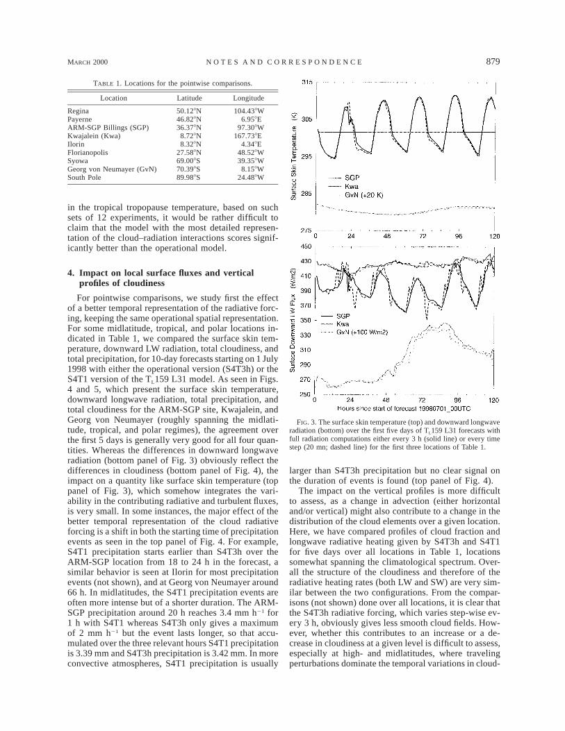
TABLE 1. Locations for the pointwise comparisons.

Location Latitude Longitude

ReginaPayerneARM-SGP Billings (SGP)Kwajalein (Kwa)IlorinFlorianopolisSyowaGeorg von Neumayer (GvN)South Pole

50.128N46.828N36.378N8.728N8.328N

27.588N69.008S70.398S89.988S

104.438W6.958E

97.308W167.738E

4.348E48.528W39.358W8.158W

24.488W

FIG. 3. The surface skin temperature (top) and downward longwaveradiation (bottom) over the first five days of TL159 L31 forecasts withfull radiation computations either every 3 h (solid line) or every timestep (20 mn; dashed line) for the first three locations of Table 1.

in the tropical tropopause temperature, based on suchsets of 12 experiments, it would be rather difficult toclaim that the model with the most detailed represen-tation of the cloud–radiation interactions scores signif-icantly better than the operational model.

4. Impact on local surface fluxes and verticalprofiles of cloudiness

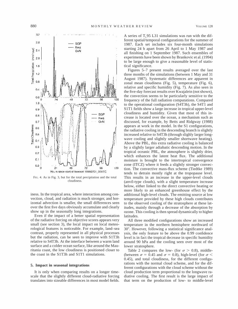
For pointwise comparisons, we study first the effectof a better temporal representation of the radiative forc-ing, keeping the same operational spatial representation.For some midlatitude, tropical, and polar locations in-dicated in Table 1, we compared the surface skin tem-perature, downward LW radiation, total cloudiness, andtotal precipitation, for 10-day forecasts starting on 1 July1998 with either the operational version (S4T3h) or theS4T1 version of the TL159 L31 model. As seen in Figs.4 and 5, which present the surface skin temperature,downward longwave radiation, total precipitation, andtotal cloudiness for the ARM-SGP site, Kwajalein, andGeorg von Neumayer (roughly spanning the midlati-tude, tropical, and polar regimes), the agreement overthe first 5 days is generally very good for all four quan-tities. Whereas the differences in downward longwaveradiation (bottom panel of Fig. 3) obviously reflect thedifferences in cloudiness (bottom panel of Fig. 4), theimpact on a quantity like surface skin temperature (toppanel of Fig. 3), which somehow integrates the vari-ability in the contributing radiative and turbulent fluxes,is very small. In some instances, the major effect of thebetter temporal representation of the cloud radiativeforcing is a shift in both the starting time of precipitationevents as seen in the top panel of Fig. 4. For example,S4T1 precipitation starts earlier than S4T3h over theARM-SGP location from 18 to 24 h in the forecast, asimilar behavior is seen at Ilorin for most precipitationevents (not shown), and at Georg von Neumayer around66 h. In midlatitudes, the S4T1 precipitation events areoften more intense but of a shorter duration. The ARM-SGP precipitation around 20 h reaches 3.4 mm h21 for1 h with S4T1 whereas S4T3h only gives a maximumof 2 mm h21 but the event lasts longer, so that accu-mulated over the three relevant hours S4T1 precipitationis 3.39 mm and S4T3h precipitation is 3.42 mm. In moreconvective atmospheres, S4T1 precipitation is usually

larger than S4T3h precipitation but no clear signal onthe duration of events is found (top panel of Fig. 4).

The impact on the vertical profiles is more difficultto assess, as a change in advection (either horizontaland/or vertical) might also contribute to a change in thedistribution of the cloud elements over a given location.Here, we have compared profiles of cloud fraction andlongwave radiative heating given by S4T3h and S4T1for five days over all locations in Table 1, locationssomewhat spanning the climatological spectrum. Over-all the structure of the cloudiness and therefore of theradiative heating rates (both LW and SW) are very sim-ilar between the two configurations. From the compar-isons (not shown) done over all locations, it is clear thatthe S4T3h radiative forcing, which varies step-wise ev-ery 3 h, obviously gives less smooth cloud fields. How-ever, whether this contributes to an increase or a de-crease in cloudiness at a given level is difficult to assess,especially at high- and midlatitudes, where travelingperturbations dominate the temporal variations in cloud-


FIG. 4. As in Fig. 3, but for the total precipitation and the totalcloudiness.

iness. In the tropical area, where interaction among con-vection, cloud, and radiation is much stronger, and hor-izontal advection is smaller, the small differences seenover the first five days obviously accumulate and clearlyshow up in the seasonally long integrations.

Even if the impact of a better spatial representationof the radiative forcing on objective scores appears verysmall (see section 3), the local impact on local meteo-rological features is noticeable. For example, land–seacontrast, properly represented in all physical processesbut the radiation, can be seen to improve with S1T3hrelative to S4T3h. At the interface between a warm landsurface and a colder ocean surface, like around the Mau-ritania coast, the low cloudiness is positioned closer tothe coast in the S1T3h and S1T1 simulations.

5. Impact in seasonal integrations

It is only when comparing results on a longer time-scale that the slightly different cloud-radiative forcingtranslates into sizeable differences in most model fields.

A series of TL95 L31 simulations was run with the dif-ferent spatial/temporal configurations for the summer of1987. Each set includes six four-month simulationsstarting 24 h apart from 26 April to 1 May 1987 andall finishing on 1 September 1987. Such ensembles ofexperiments have been shown by Brankovic et al. (1994)to be large enough to give a reasonable level of statis-tical significance.

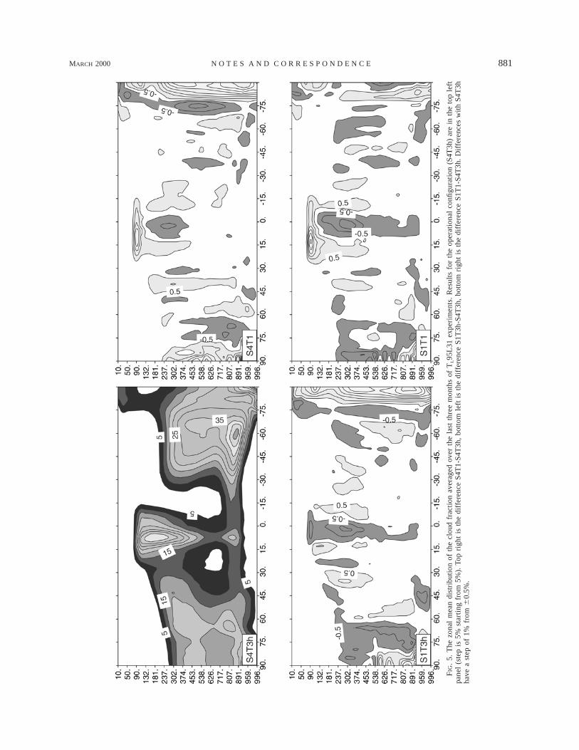
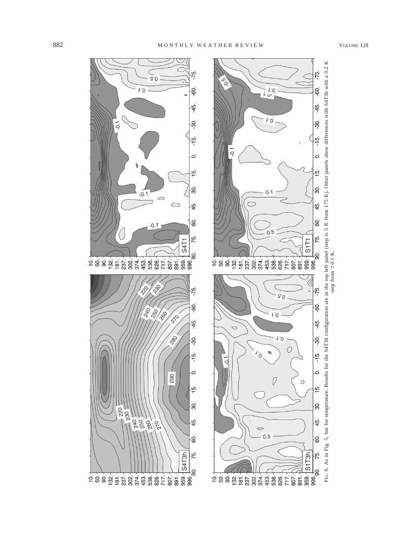
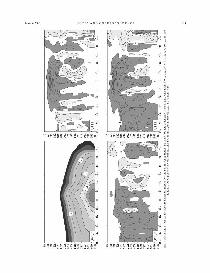
Figures 5–7 present results averaged over the lastthree months of the simulations (between 1 May and 31August 1987). Systematic differences are apparent inzonal mean cloudiness (Fig. 5), temperature (Fig. 6),relative and specific humidity (Fig. 7). As also seen inthe five-day forecast results over Kwajalein (not shown),the convection seems to be particularly sensitive to thefrequency of the full radiation computations. Comparedto the operational configuration (S4T3h), the S4T1 andS1T1 fields show a large increase in tropical upper-levelcloudiness and humidity. Given that most of this in-crease is located over the ocean, a mechanism such asdiscussed, for example, by Betts and Ridgway (1988)appears at work in the model. In the S1 configurations,the radiative cooling in the descending branch is slightlyincreased relative to S4T3h (through slighly larger long-wave cooling and slightly smaller shortwave heating).Above the PBL, this extra radiative cooling is balancedby a slightly larger adiabatic descending motion. In thetropical oceanic PBL, the atmosphere is slightly drier,which enhances the latent heat flux. The additionalmoisture is brought to the intertropical convergencezone (ITCZ) where it feeds a slightly stronger convec-tion. The convective mass-flux scheme (Tiedtke 1989)tends to detrain mostly right at the tropopause level.This results in an increase in the upper-level clouds(anvil-type clouds), with a slight temperature increasebelow, either linked to the direct convective heating ormore likely to an enhanced greenhouse effect by theadditional high-level clouds. The emitting source at lowtemperature provided by these high clouds contributesto the observed cooling of the stratosphere at these lat-itudes, mainly through a decrease of the absorption byozone. This cooling is then spread dynamically to higherlatitudes.

All three modified configurations show an increasedtemperature in the northern hemisphere northward of308. However, following a statistical significance anal-ysis, the only feature to be above the 0.99 confidencelevel is in fact the tropical decrease in specific humidityaround 90 hPa and the cooling seen over most of thelower stratosphere.

Table 2 compares the low- (for s . 0.8), middle-(between s 5 0.45 and s 5 0.8), high-level (for s ,0.45), and total cloudiness, for the different configu-rations with the normal cloud scheme, and for the dif-ferent configurations with the cloud scheme without thecloud production term proportional to the longwave ra-diative cooling. The first result is the large impact ofthat term on the production of low- to middle-level


FIG

.5.

The

zona

lm

ean

dist

ribu

tion

ofth

ecl

oud

frac

tion

aver

aged

over

the

last

thre

em

onth

sof

TL95

L31

expe

rim

ents

.R

esul

tsfo

rth

eop

erat

iona

lco

nfigu

rati

on(S

4T3h

)ar

ein

the

top

left

pane

l(s

tep

is5%

star

ting

from

5%).

Top

righ

tis

the

diff

eren

ceS

4T1-

S4T

3h,

bott

omle

ftis

the

diff

eren

ceS

1T3h

-S4T

3h,

bott

omri

ght

isth

edi

ffer

ence

S1T

1-S

4T3h

.D

iffe

renc

esw

ith

S4T

3hha

vea

step

of1%

from

60.

5%.


FIG

.6.

As

inF

ig.

5,bu

tfo

rte

mpe

ratu

re.

Res

ults

for

the

S4T

3hco

nfigu

rati

onar

ein

the

top

left

pane

l(s

tep

is5

Kfr

om17

5K

).O

ther

pane

lssh

owdi

ffer

ence

sw

ith

S4T

3hw

ith

a0.

2K

step

from

60.

1K

.


FIG

.7.

As

inF

ig.

5,bu

tfo

rth

esp

ecifi

chu

mid

ity.

Res

ults

for

the

S4T

3hco

nfigu

rati

onar

ein

the

top

left

pane

l(l

evel

sar

ein

g/kg

wit

hli

nes

at0.

1,0.

2,0.

4,0.

7,1,

2,4,

7,10

,12

,15

and

20g/

kg).

Oth

erpa

nels

show

diff

eren

ces

wit

hS

4T3h

asD

q/q

inpe

rcen

t(s

tep

is2%

from

61%

).


TABLE 2. Cloud cover at various levels with the different spatio–temporal configurations and two versions of the cloud scheme.

Reference S4T3h S4T1 S1T3h S1T1

HCCMCCLCCTCC

35.9526.3823.7662.17

36.1326.4023.3962.27

35.9226.7423.6862.40

36.6026.4123.7462.83

No LWHCCMCCLCCTCC

34.5721.8817.5755.26

34.9421.4117.5255.35

34.0021.7517.0054.51

34.9521.4017.2855.07

clouds (about 6% and 5%, respectively, whatever thespatio–temporal configuration). Second, although thereare some systematic differences between the differentconfigurations, with the radiation at every time stepleading to larger high-level and total cloud amounts, thesignals remain rather small on a global basis. Moreover,most of the differences brought by the different config-urations do not appear at specified locations.

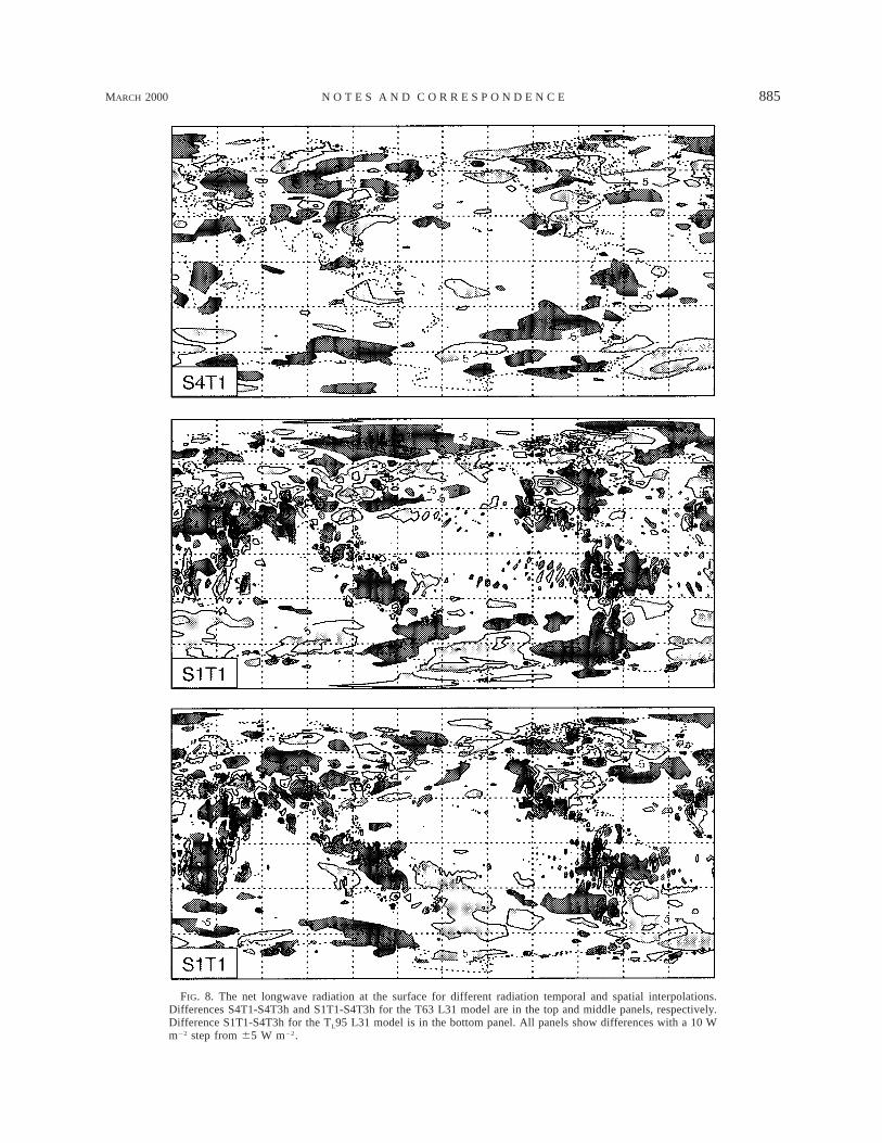
When looking at surface fluxes, one can see the ben-efit brought by the linear grid approach of Hortal (1998).Figure 8 compares the surface net longwave flux forvarious configurations (S4T3h, S4T1, and S1T1), for aspectral model with a T63 truncation and the more re-cent TL95 equivalent from the point of view of the phys-ical calculations but with more terms in computing thedynamical tendencies. When full radiation is computedfor all grid-points (S1 configurations), the spectral na-ture of the model is apparent in all physical fieldsthrough a modulation of the surface pressure. This, inturn, affects the vertical column of the various absorbersand finally shows up as a (slight) modulation of thefields. This effect is particularly evident in the surfacenet longwave radiation (Fig. 8), but also in the surfacenet shortwave radiation (not shown). This can be seenin the middle panel of Fig. 8 that presents, for the T63L31 model, the difference in surface net longwave ra-diation between S4T3h and S1T1. Comparison betweenS1T3h-S4T3h (not shown but similar to S1T1-S4T3h)and S4T1-S4T3h (top panel of Fig. 8) confirms that theripples appear because of the radiation computations areperformed at every grid point. In this respect, the lineargrid approach significantly reduces this problem of oro-graphic ripples (compare middle and bottom panels ofFig. 8), but does not make it fully disappear. It must benoticed that the radiation configuration used for the op-erational forecasts at ECMWF with its S4 horizontalsampling hides the problem. By providing a smootherspatial radiative forcing, this configuration also smoothsout other physical fluxes and tendencies.

6. Impact on operational analyses

The operational analyses rely on 6-h first-guess fore-casts, for which the full radiation is called every hour,

so that the direct effect of the temporal interpolationdiscussed above is three times smaller. We carried outa series of analyses from 19980630 1800 UTC to19980706 1800 UTC with the operational TL319 L31model including all four radiation configurations. Giventhe forcing by observations, the impact of the variousradiation configurations is very much smaller than inthe free-running 10-day forecasts and four-month sim-ulations. However, where (or when, as it is sometimesthe case at 0600 or 1800 UTC) the density of obser-vations gets smaller, the influence of the first-guess fore-cast gets larger. Obviously the major impact (notshown), in both specific humidity and temperature, isseen where the density of observations is low like overAntarctica, and to a lesser extent in the northern polarregion. In these areas, the differences between the var-ious configurations can be as high as 0.15 K in tem-perature and 5% in relative humidity. Otherwise, overthe rest of the atmosphere, the impact on the zonalmeans of temperature and humidity remains quite small,with maximum differences occuring in the upper partof the ITCZ, reaching at most 0.05 K in temperature,and 2% in relative humidity over patchy areas showingno particular organization.

Although the cloudiness is not an analyzed quantity,the changes in analyzed humidity and temperature havean impact on the cloudiness. Cloudiness over Antarcticadisplays variations up to 5% depending on the config-uration. Otherwise, the upper troposphere in the equa-torial region shows up as the area most sensitive areato these small changes in analyzed moisture and tem-perature with maximum decrease of 2% in zonal meancloudiness around 200 hPa.

7. Concluding remarks and climate sensitivity

To put in perspective the differences introduced bythe radiation temporal/spatial interpolation scheme, thesignal is usually smaller than the signal seen whenchanging details of the cloud microphysical processes,cloud radiative properties or cloud overlap assumptions.At present, in a weather forecast environment, the hugeincrease in computer time introduced by decreasing thetime frequency and/or spatial sampling of the full ra-diation computations could only become acceptable ifthese computations were handled with a much moreefficient method, such as the neural network approach(Chevallier et al. 1998). The main conclusions are thefollowing:

R the model appears to be much more sensitive to econ-omies in the temporal than in the spatial descriptionof the cloud–radiation interactions;

R in terms of the 10-day forecast quality, the anomalycorrelation of geopotental displays little sensitivity tothe spatial/temporal representation;

R the configuration presently used for running the op-


FIG. 8. The net longwave radiation at the surface for different radiation temporal and spatial interpolations.Differences S4T1-S4T3h and S1T1-S4T3h for the T63 L31 model are in the top and middle panels, respectively.Difference S1T1-S4T3h for the TL95 L31 model is in the bottom panel. All panels show differences with a 10 Wm22 step from 65 W m22.


TABLE 3. Feedback and sensitivity parameters derived from TL95L31 perpetual July simulations.

Configuration Clear sky Total sky Ratio

S4T3hS4T1S1T3hS1T1

0.5040.4760.4610.452

0.6570.7670.6930.777

1.3041.6111.5041.718

erational data assimilation introduces little bias on theresults of the analyses;

R in seasonal simulations, the impact is much strongerwith the increase in temporal resolution leading to adecrease in upper-tropospheric moisture in the Trop-ics, a larger amount of tropical high clouds, and acolder stratosphere, whereas the increase in spatialresolution increases the temperature over most of thetroposphere.

All results presented here are specific to the ECMWFmodel. The question is whether the ECMWF modelmight be more or less sensitive to the temporal (andspatial) interpolation than other general circulation mod-els are. Most, if not all, climate and numerical weatherprediction models have to use some time-sampling strat-egy for reducing the cost of the radiative computations.Studies by Wilson and Mitchell (1986), Charlock et al.(1988), and Smith and Vonder Haar (1991) indicatedthat the weak coupling among cloudiness, radiation, andthe hydrological cycle, existing in models with a di-agnostic cloud scheme, overestimated the variability oftop-of-the-atmosphere radiation fluxes when comparedto satellite observations of the radiation budget. There-fore, models using diagnostic cloud schemes are likelyto show at least a similar dependence on the temporalsampling used for radiative computations.

Tiedtke (1994) showed that the prognostic cloud rep-resentation, with a much stronger coupling of the cloud-iness to the physical processes, was improving the timecontinuity of the cloud fields, particularly with respectto the anvil-topped convective cloud systems. This par-ticular prognostic cloud scheme relates the formation,maintenance, and dissipation of cloud volume and cloudwater to most parts of the physics package, as it ex-plicitly uses the tendencies from convection, large-scalecondensation, vertical diffusion, and radiation in theprognostic equations for cloud water and cloud fraction.Including the radiative tendencies might make theECMWF model more sensitive to the radiation inter-polation scheme than a model with clouds whose watercontent is prognosed but cloud fraction is diagnosedfrom relative humidity [as in Sundqvist (1988) or Smith(1990)]. Relative humidity is a much smoother quantityin both time and space than most of the outputs of thedynamical and physical processes used as precursors/predictors of cloud volume and cloud water in theECMWF scheme. Other prognostic cloud schemes(Fowler et al. 1996) are also linking the cloud waterand cloud mass (fraction) more directly to the individualphysical tendencies. It would be interesting to seewhether the effects of the spatial/temporal interpolationdescribed here are also found in other weather forecastor climate models, as most models cannot afford a ra-diation scheme fully interactive with the rest of the phys-ical parametrizations.

As seen in sections 5 and 6, the intertropical hightroposphere is the area where the largest changes in

temperature, humidity, and cloudiness occur whenchanging the configuration of the radiation computa-tions. So, we looked at the impact of the temporal/spatialinterpolation scheme on the sensitivity of the model toa change in sea surface temperature computed followingthe procedure outlined in Cess et al. (1990). A numberof TL95 L31 simulations were performed for the fourtemporal/spatial configurations for perpetual July 1987conditions, with fixed SST with a plus or minus 2 Kincrement, and fixed sea ice, soil moisture, and snowcover maintained at 19870701 conditions. The clear andtotal sky feedback and sensitivity parameters for the fourconfigurations used here are presented in Table 3. Asimple interpretation of these results is that, throughhigher spatial and temporal resolution, the cloudiness,and therefore, the top-of-the-atmosphere radiation fieldsare more likely to follow the intensification of the con-vective activity brought by the increased sea surfacetemperature over the ocean, thus increasing the sensi-tivity parameter. This result also shows how sensitiveCess’s methodology is to what can be thought of asrelatively intricate details of the cloud–radiation inter-actions and, as such, at least in the context of theECMWF model, casts doubt on the validity of the ex-ercise. Again, it would be interesting to see whether the(spatial and) temporal interpolation used in other globalcirculation models also have an impact on the climatesensitivity parameter.

Acknowledgments. Drs. Anton Beljaars and MartinMiller are thanked for reviewing the manuscript.

REFERENCES

Betts, A. K., and W. Ridgway, 1988: Coupling of the radiative, con-vective, and surface fluxes over the equatorial Pacific. J. Atmos.Sci., 45, 522–536., and , 1989: Climatic equilibrium of the atmospheric con-vective boundary layer over a tropical ocean. J. Atmos. Sci., 46,2621–2641.

Brankovic, C., T. N. Palmer, and L. Ferranti, 1994: Predictability ofseasonal atmospheric variations. J. Climate, 7, 217–237.

Cess, R. D., and Coauthors, 1990: Intercomparison and interpretationof climate feedback processes in seventeen atmospheric generalcirculation models. J. Geophys. Res., 95D, 16 601–16 617.

Charlock, T. P., K. M. Cattany-Carnes, and F. Rose, 1988: Fluctuationstatistics of outgoing longwave radiation in a general circulationmodel and in satellite data. Mon. Wea. Rev., 116, 1540–1554.

Chevallier, F., F. Cheruy, Z.-X. Li, and N. A. Scott, 1998: A neuralnetwork approach for a fast and accurate computation of a long-wave radiation budget. J. Appl. Meteor., 37, 1385–1397.

Ebert, E. E., and J. A. Curry, 1992: A parametrisation of ice cloud


optical properties for climate models. J. Geophys. Res., 97D,3831–3836.

Fowler, L. D., D. A. Randall, and S. A. Rutledge, 1996: Liquid andice cloud microphysics in the CSU general circulation model:Part I: Model description and simulated microphysical processes.J. Climate, 9, 489–529.

Gregory, D., J.-J. Morcrette, C. Jakob, and A. Beljaars, 1998: Intro-duction of revised radiation, convection, and vertical diffusionschemes into cycle 18r3 of the ECMWF integrated forecastingsystem. ECMWF Tech. Memo. No. 254., 39 pp.

Hortal, M., 1998: TL319 resolution and revised orographies. ECMWFResearch Department Memo. R60.5/MH/23, 18 pp., and A. J. Simmons, 1991: Use of reduced Gaussian grids inspectral models. Mon. Wea. Rev., 119, 1057–1074.

Jakob, C., 1994: The impact of the new cloud scheme on ECMWF’sIntegrated Forecast System. Proc. ECMWF Workshop on Mod-elling, Validation and Assimilation of Clouds, Reading, UnitedKingdom, ECMWF, 277–294.

Morcrette, J.-J., 1999: Effects of the temporal and spatial samplingof radiation fields on the ECMWF forecasts and analyses.ECMWF Tech. Memo. No. 277, 33 pp.

Rabier, F., and Coauthors, 1997: Recent experimentation on 4D-Var

and first results from a simplified Kalman filter. ECMWF Tech.Rep. 240, 42 pp.

Smith, L. D., and T. H. Vonder Haar, 1991: Cloud-radiation inter-actions in a general circulation model: Impact upon the planetaryradiation balance. J. Geophys. Res., 96D, 893–914.

Smith, R. N. B., 1990: A scheme for predicting layer clouds and theirwater content in a general circulation model. Quart. J. Roy.Meteor. Soc., 116, 435–460.

Sundqvist, H., 1988: Parameterization of condensation and associatedclouds in models for weather prediction and general circulationsimulation. Physically Based Modelling and Simulation of Climateand Climate Change, M. E. Schlesinger, Ed., Kluwer, 433–461.

Tiedtke, M., 1989: A comprehensive mass-flux scheme for cumulusparameterization in large-scale models. Mon. Wea. Rev., 117,1779–1800., 1993: Representation of clouds in large-scale models. Mon.Wea. Rev., 121, 3040–3061., 1994: Critical aspects of cloud parametrization in large-scalemodels. Proc. ECMWF Workshop on Modelling, Validation andAssimilation of Clouds, Reading, United Kingdom, ECMWF, 22–42.

Wilson, C. A., and J. F. B. Mitchell, 1986: Diurnal variation andcloud in a general circulation model. Quart. J. Roy. Meteor.Soc., 112, 347–369.

On the Effects of the Temporal and Spatial Sampling of Radiation Fields on the ECMWF Forecasts and...

Documents

Transcript of On the Effects of the Temporal and Spatial Sampling of Radiation Fields on the ECMWF Forecasts and...