Design and Characterization of a Concentrating Solar Simulator

Design and Characterization of a

Concentrating Solar Simulator

A DISSERTATION

SUBMITTED TO THE FACULTY OF THE GRADUATE SCHOOL

OF THE UNIVERSITY OF MINNESOTA

BY

Katherine R. Krueger

IN PARTIAL FULFILLMENT OF THE REQUIREMENTS

FOR THE DEGREE OF

DOCTOR OF PHILOSOPHY

Dr. Jane H. Davidson, Dr. Wojciech Lipiński, Advisers

July 2012

i

Acknowledgements

I would like to thank the following people for their contributions to this work:

My advisors, Dr. Jane H. Davidson and Dr. Wojciech Lipiński, for their guidance and

encouragement to strive for scientific rigor and excellence

Dr. Patrick Coray for use of his flux measurement software (T-Flux) and assistance with

its modifications

Dr. Jörg Petrasch for the use of VeGas

My colleagues who helped with flux measurement acquisition: Daryl Lee, Eung Joon

Lee, Peter Krenzke, and Elizabeth Sefkow

All of my colleagues in the solar lab between 2008 and 2012 who participated in rigorous

discussions and have given helpful feedback

The funding provided by the University of Minnesota Graduate School, the Initiative for

Renewable Energy and the Environment, and the College of Science and Engineering is greatly

appreciated.

I would also like to thank Dr. Robert Palumbo, for inspiring me to get started in solar research in

the first place and beginning my engineering toolbox.

Soli Deo gloria

ii

Dedication

To my family, especially Mom, Dad, Karl, Karen, and Aunt Joanna (ROL), for all of your

unending love and support.

To the community and the Cantorei at Mount Olive Lutheran Church in Minneapolis: whether

you know it or not, your care and encouragement has meant the world to me.

To all of the numerous friends and unnamed family members who have encouraged me,

commiserated with me, stayed up late doing homework with me, prayed for me, or just listened:

thank you.

And most importantly, to Matt, for loving me and believing in me when it seemed like no one

else did. You’re my rock, my other half, my helpmate, and I couldn’t have gotten this far without

you by my side. You’re the best.

iii

Abstract

A concentrating solar simulator is a laboratory-scale tool that is useful in the development of

processes to generate solar fuels. Such a device, which produces a concentrated radiative output

replicating that of a solar dish, has been designed, built, and characterized at the University of

Minnesota to facilitate the testing of prototype solar receivers and reactors. The concentrating

solar simulator consists of seven commonly-focused radiation units, each consisting of a xenon

arc lamp close-coupled to a reflector in the shape of an ellipsoid of revolution. A systematic

design procedure has been developed as part of this work, which involves determining the

location and orientation of each of the radiation units by requiring that the target focal points of

all reflectors coincide. A set of unique geometric relations have been developed that ensure this

requirement on a general scale and provide the framework for further designs by allowing the

specification of detailed practical requirements dealing with the space available and

manufacturability concerns. After the location and orientation of each of the lamp-reflector

modules is established, the shape of the reflector is optimized with the use of a Monte Carlo ray

tracing model. The shape of the ellipsoidal reflector is varied by the eccentricity, and sensitivity

analyses are carried out to determine the effect of the reflector specular error and effective arc

size and shape on the resulting flux distribution and magnitude. The completed facility consists of

a dual enclosure specially designed to protect the researchers and the simulator, the array of

lamps and reflectors, and the electrical systems necessary to power and control the lamps.

The radiative output of the solar simulator constitutes the energy input to the prototype solar

receivers and reactors, and therefore must be well-characterized. The output has been measured

with respect to its spatial and temporal variations by using an optical technique in which a CCD

camera views radiation reflected from a water-cooled Lambertian target through neutral density

filters and a lens. The image recorded by the camera is calibrated such that the recorded

grayscales correspond to measured values of incident radiative flux, as measured by a circular foil

heat flux gage that has been calibrated in-house. Using this method, it was determined that the

solar simulator can output up to 9.2 0.4 kW of thermal power to a focal area 60 mm in diameter,

corresponding to an average flux of 3240±390 kW m-2

. The peak flux, as averaged over a 10 mm

diameter focal area, is 7300±890 kW m-2

. The UMN solar simulator facility is an excellent tool

for testing prototype solar receivers and reactors on a laboratory scale.

iv

Table of Contents Acknowledgements .................................................................................................................... i

Dedication ................................................................................................................................. ii

Abstract .................................................................................................................................... iii

Table of Contents ..................................................................................................................... iv

List of Tables ........................................................................................................................... vii

List of Figures ........................................................................................................................ viii

Nomenclature ......................................................................................................................... xiii

Chapter 1 Introduction ............................................................................................................... 1

1.1 Motivation and Objectives .............................................................................................. 1

1.2 Approach ....................................................................................................................... 10

1.2.1 Design ..................................................................................................................... 10

1.2.2 Fabrication .............................................................................................................. 11

1.2.3 Characterization ...................................................................................................... 12

1.3 Significance ................................................................................................................... 13

Chapter 2 Solar Simulator Design ........................................................................................... 14

2.1 Lamp Selection and Spectral Considerations ................................................................ 15

2.2 Geometric Relations ...................................................................................................... 19

2.3 Parameter Selection ....................................................................................................... 21

2.4 Summary ....................................................................................................................... 24

Chapter 3 Reflector Optimization and Predicted Simulator Performance............................... 25

3.1 Monte Carlo Ray Tracing Method ................................................................................ 25

3.1.1 Assumptions ........................................................................................................... 26

3.1.2 Fundamental Monte Carlo principles ..................................................................... 26

3.1.3 Ray emission relations ............................................................................................ 27

3.1.4 Ray and surface interactions ................................................................................... 29

3.2 Model of the Lamp-Reflector Unit ................................................................................ 31

3.2.1 Xenon arc ............................................................................................................... 32

3.2.2 Reflector ................................................................................................................. 34

3.2.3 Target ...................................................................................................................... 37

3.3 Single Reflector Optimization ....................................................................................... 38

3.3.1 Parameter identification.......................................................................................... 40

3.3.2 Accuracy Considerations ........................................................................................ 48

3.4 Summary ....................................................................................................................... 49

Chapter 4 Completed Facility .................................................................................................. 50

4.1 Dual Enclosure .............................................................................................................. 51

4.2 Radiation Units .............................................................................................................. 57

4.3 Summary ....................................................................................................................... 60

Chapter 5 Measurement and Calibration Techniques.............................................................. 61

5.1 Measurement Method & Instrumentation ..................................................................... 61

5.2 Assumptions .................................................................................................................. 64

5.2.1 Directional considerations ...................................................................................... 64

5.2.2 Spectral considerations ........................................................................................... 66

5.3 Calibration Methods ...................................................................................................... 69

5.3.1 Circular foil heat flux gage ..................................................................................... 69

5.3.2 CCD camera and Lambertian target ....................................................................... 76

Chapter 6 Measured Solar Simulator Performance ................................................................. 81

6.1 Measurement Methods .................................................................................................. 81

6.1.1 Spatial flux ............................................................................................................. 81

6.1.2 Flux map superposition .......................................................................................... 82

6.1.3 Temporal characterization ...................................................................................... 83

6.1.4 Adaptive characterization ....................................................................................... 83

6.2 Results ........................................................................................................................... 84

6.2.1 Individual radiation units ........................................................................................ 84

6.2.2 Complete solar simulator performance .................................................................. 88

6.2.3 Flux map superposition .......................................................................................... 91

6.2.4 Temporal variations ................................................................................................ 92

6.2.5 Adaptive characterization ....................................................................................... 94

6.3 Summary ....................................................................................................................... 97

Chapter 7 Summary & Conclusions ........................................................................................ 99

7.1 Summary ....................................................................................................................... 99

7.2 Key Contributions ....................................................................................................... 101

7.3 Recommendations for Future Work ............................................................................ 102

Bibliography .......................................................................................................................... 104

Appendix A. Notes on the Specular Error Definition ........................................................ 109

A.1 Modifying the Normal by Polar and Azimuth Angles ................................................ 109

A.2 Modifying the Tangential Components of the Reflected Ray .................................... 110

Appendix B. Manual for Focusing the Solar Simulator .................................................... 113

Appendix C. Solar Simulator Operating Manual .............................................................. 116

Appendix D. Heat Flux Gage Thermal Analysis ............................................................... 127

Appendix E. Optical Flux Uncertainty Analysis ............................................................... 131

Appendix F. Comparison Data for Two Lambertian Targets ........................................... 133

List of Tables

Table 1.1: Design goals for the UMN solar simulator ................................................................... 11

Table 2.1: Geometric constraints on the solar simulator design .................................................... 19

Table 2.2: Final parameters of the lamp-reflector modules ........................................................... 23

Table 3.1: Cumulative density functions for , , and for isotropic volumetric emission ......... 28

Table 3.2: Coordinates of the arc center and foot points of the ellipsoid and cylindrical arc in the

global system centered at the target focal point. The eccentricity portrayed here is 0.890. .... 33

Table 3.3: Geometric parameters of the inner surface of a single reflector ................................... 43

Table 4.1: Approximate room temperature increase for selected thermal loads ............................ 55

Table 5.1: Values of total hemispherical absorptivity with varying incident spectra .................... 71

Table 6.1: Summary of individual radiation unit outputs .............................................................. 86

Table 6.2: Comparison of the UMN solar simulator (all 7 units operating) flux distribution to that

generated by the EURODISH [14] .......................................................................................... 91

Table 6.3: Transfer efficiency, flux non-uniformity, radiative power, and average flux incident in

60- and 100-mm diameter focal areas for measured and modeled flux distributions. Modeled

distributions were generated with a cylindrical arc 2 mm in radius and 6.3 mm long. ........... 97

Table D.1: Values of measured parameters and constants used to calculate the incident heat flux

by the calorimetric method .................................................................................................... 128

Table D.2: List of constants used in the heat flux gage thermal analysis .................................... 128

Table E.1: Values of the incident radiative fluxes, mean grayscales, and uncertainties in each used

to calibrate the optical calibration curve slope ...................................................................... 131

Table F.1: Summary of average grayscales in a 25 mm region of interest, measured using all

seven radiation units and comparing the plain target to the target with a hole. .................... 133

viii

List of Figures

Fig. 1.1: Schematic drawings of three types of solar concentrating facilities (a) parabolic trough

(b) solar dish and (c) central receiver. Images courtesy of Steinfeld & Palumbo [2]. .............. 2

Fig. 1.2: Sample flux distributions taken in the focal planes of two different solar dish

concentrators (a) DISTAL II North and (b) EURODISH South. The crosshairs represent the

center of the ideally-focused concentrator and the flux levels are displayed on a logarithmic

scale after being normalized to a standard insolation of 1000 W m-2

[23] ................................ 5

Fig. 1.3: Schematic of the solar simulator at the Jet Propulsion Laboratory [25] ............................ 7

Fig. 1.4: Radiative flux uniformity output by the solar simulator at the Jet Propulsion Laboratory

[25] ............................................................................................................................................ 8

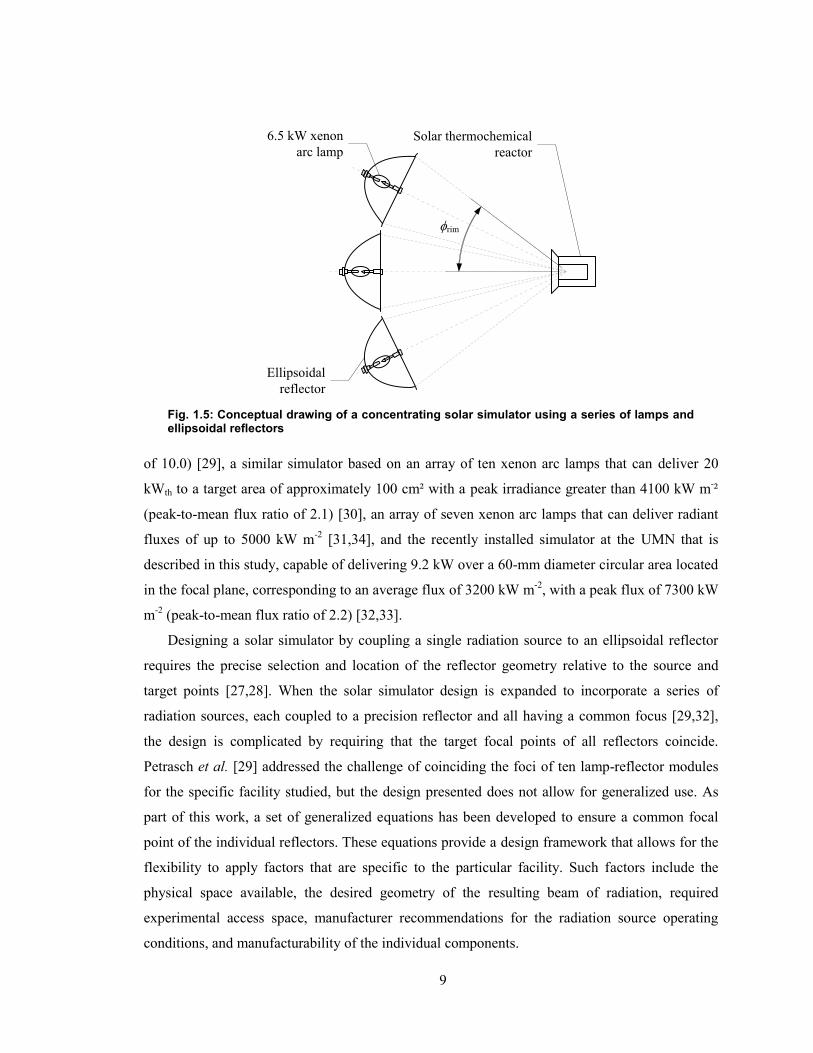
Fig. 1.5: Conceptual drawing of a concentrating solar simulator using a series of lamps and

ellipsoidal reflectors .................................................................................................................. 9

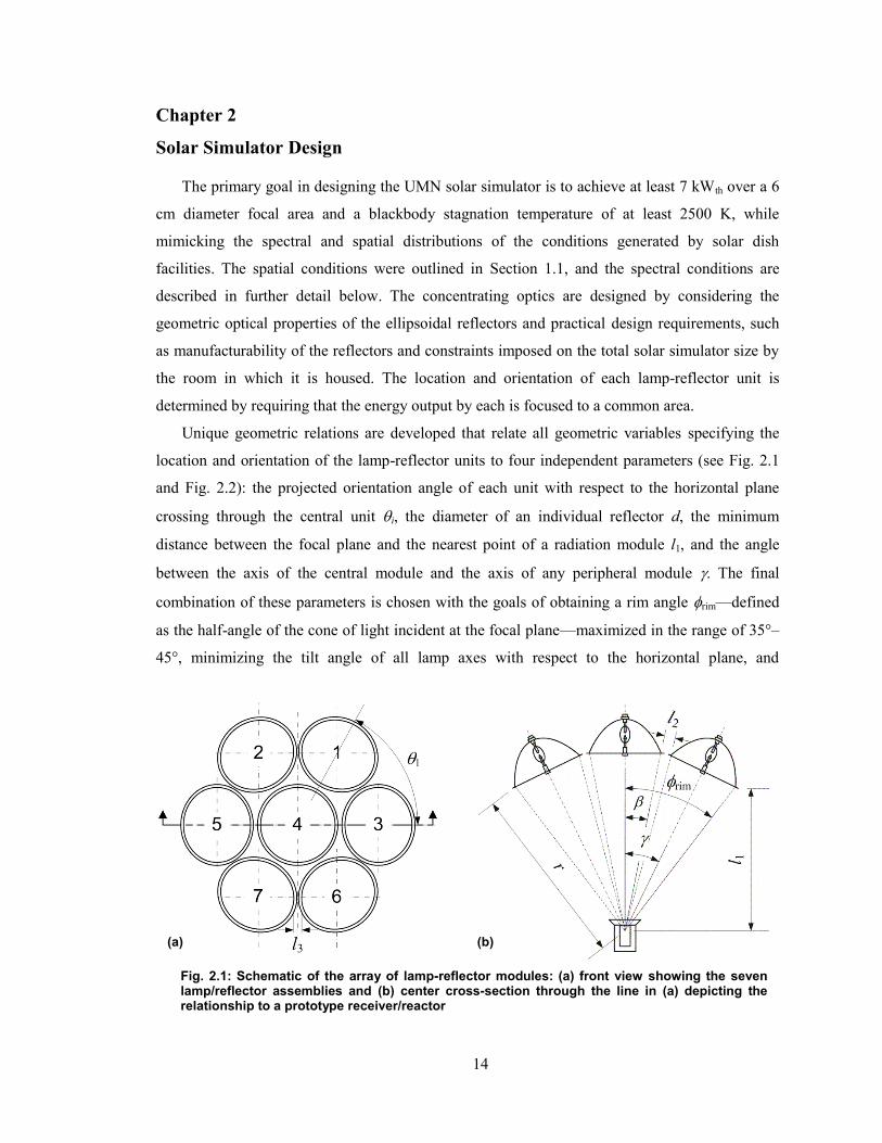
Fig. 2.1: Schematic of the array of lamp-reflector modules: (a) front view showing the seven

lamp/reflector assemblies and (b) center cross-section through the line in (a) depicting the

relationship to a prototype receiver/reactor ............................................................................. 14

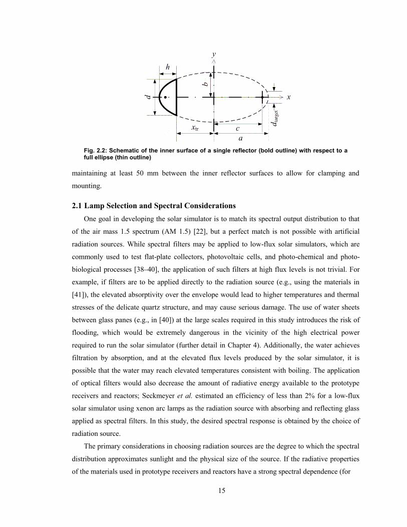
Fig. 2.2: Schematic of the inner surface of a single reflector (bold outline) with respect to a full

ellipse (thin outline) ................................................................................................................. 15

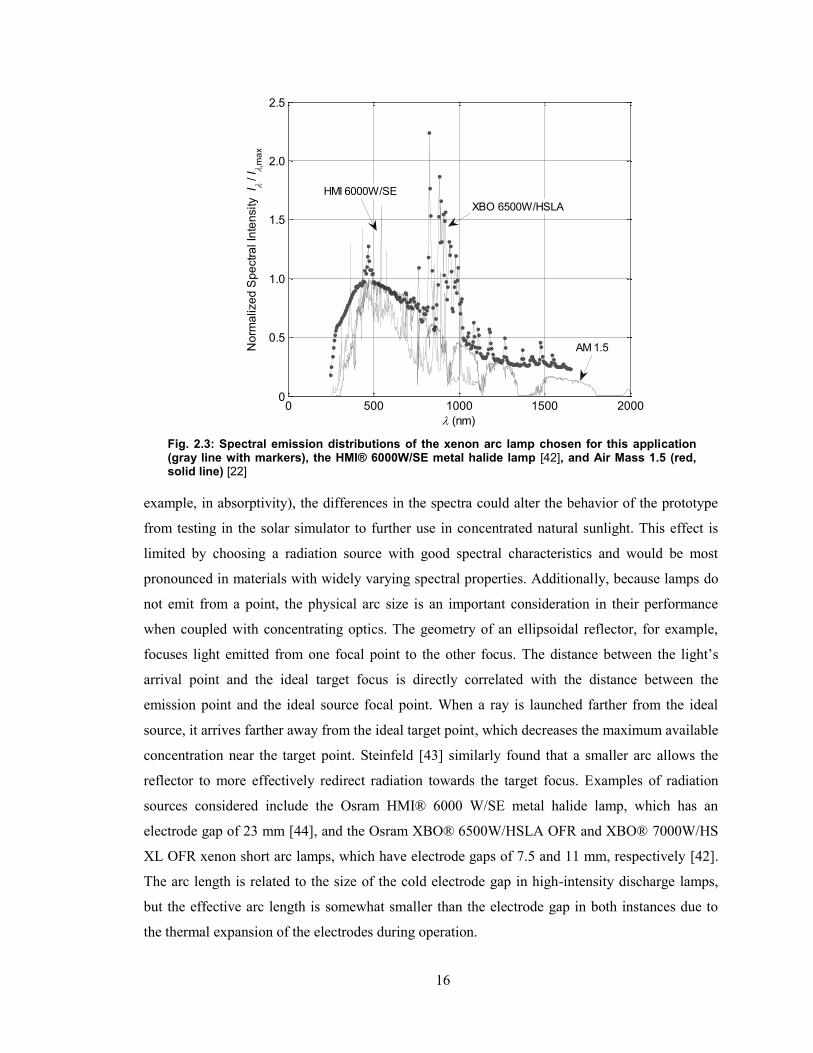
Fig. 2.3: Spectral emission distributions of the xenon arc lamp chosen for this application (gray

line with markers), the HMI® 6000W/SE metal halide lamp [42], and Air Mass 1.5 (red,

solid line) [22] ......................................................................................................................... 16

Fig. 2.4: Analytical relationships among rim, , 1, l3, and d with l1 = 1.45 m. The shaded areas

indicate values that satisfy the design requirements. ............................................................... 22

Fig. 2.5: Analytical relationships among rim, , 1, l3, and l1 with d = 0.75 m. The shaded areas

indicate values that satisfy the design requirements ................................................................ 22

Fig. 3.1: The specular error is defined as the standard deviation s of a distribution of the cone

angle s measured from the normal of a perfectly smooth reflector surface ( n ) to the normal

of a real reflector surface ( *n ) ................................................................................................. 31

Fig. 3.2: Schematic of a cylindrical source, including the defining attributes of length L, outer

radius ro, and directional vector v

.......................................................................................... 32

Fig. 3.3: Schematic of a two-dimensional ellipse, to be rotated about the x-axis to form a three-

dimensional ellipsoidal reflector. This schematic depicts variables that are specific to the ray-

tracing model, as opposed to the geometric factors shown in Fig. 2.2. ................................... 34

Fig. 3.4: Schematic of a discretized circular disk used as the target in the model of the UMN solar

simulator .................................................................................................................................. 37

Fig. 3.5: Flowchart of the Monte Carlo method for thermal radiative surface transport among the

components of the UMN solar simulator ................................................................................ 39

file:///C:/Users/Katie/Documents/UMN%20Research/Degree%20Program/Dissertation/WholeThing.docx%23_Toc329786397

file:///C:/Users/Katie/Documents/UMN%20Research/Degree%20Program/Dissertation/WholeThing.docx%23_Toc329786397

Fig. 3.6: Transfer efficiency and flux standard deviation on (a) 6 cm and (b) 10 cm diameter

targets. The solid lines correspond to transfer efficiency, , and the dashed lines correspond

to flux standard deviation, f ................................................................................................... 41

Fig. 3.7: Flux maps for the geometry listed in Table 2.1 and Table 2.2 with eccentricity e = 0.890

and varying values of specular error: (a) s = 0 mrad (b) s = 7.07 mrad (c) s = 14.14 mrad;

and with specular error s = 7.07 mrad and varying values of eccentricity: (d) e = 0.850, (e) e

= 0.900, (f) e = 0.925. The inner circle is 6 cm in diameter and the outer circle is 10 cm in

diameter. Note that the scale differs for plot (a)–(c) ............................................................... 42

Fig. 3.8: Variation of transfer efficiency, , with reflector specular error, s, and target radius, rtar

for the geometry listed in Table 2.1, Table 2.2 and Table 3.3 ................................................. 44

Fig. 3.9: Variation of transfer efficiency, (solid line), and flux standard deviation, f (dashed

line), with target radius for the final geometry (Table 3.3) and s = 7.07 mrad using 108 rays

per lamp ................................................................................................................................... 45

Fig. 3.10: Sectional cuts of flux showing symmetry for the geometry listed in Table 2.1 and Table

2.2 with eccentricity e = 0.890 and varying values of specular error: (a) s = 0 mrad (b) s =

7.07 mrad (c) s = 14.14 mrad; and with specular error s = 7.07 mrad and varying values of

eccentricity: (d) e = 0.850, (e) e = 0.900, (f) e = 0.925. The inner circle is 6 cm in diameter

and the outer circle is 10 cm in diameter. Note that the scale differs between plots (a)–(c) and

(d)–(f) ...................................................................................................................................... 46

Fig. 3.11: Cumulative average flux (solid line) and power (dashed line) as a function of the target

radius for the geometry described in Table 2.1, Table 2.2, and Table 3.3 with s = 7.07 mrad

................................................................................................................................................. 47

Fig. 3.12: Diagram of lines of equal brilliance of a xenon arc lamp similar to that used in the

UMN solar simulator [51] ....................................................................................................... 47

Fig. 3.13: Cumulative average flux curves for varying arc size and geometry.............................. 48

Fig. 4.1: Photograph depicting the final solar simulator fabrication, including the simulator

support structure, enclosure, and control panel ....................................................................... 50

Fig. 4.2: Overhead view sketch of the new two-room enclosure in ME 1134 designed to house the

solar simulator ......................................................................................................................... 52

Fig. 4.3: Side section view of the two-room enclosure designed and built to house the solar

simulator, facing west. ............................................................................................................. 53

Fig. 4.4: Photograph of the interior northwest portion of the dual enclosure ................................ 54

Fig. 4.5: Photograph of the north and east interior portions of the solar simulator enclosure ....... 54

Fig. 4.6: Photographs of the (a) front and (b) profile of a completed radiation unit ...................... 57

Fig. 4.7: Cross-sectional drawing of the final reflector geometry, including mounting flanges and

lamp access hole. All dimensions are in mm. Image provided by Kinoton, GmbH ............... 58

Fig. 4.8: Solid model of the complete simulator design, including the support structures and the

location of the rectifiers. Rendering provided by Kinoton, GmbH ......................................... 59

Fig. 5.1: Schematic of the optical flux measurement system. Note that the schematic location of

the CCD camera does not represent its actual location in the completed facility. .................. 62

Fig. 5.2: Photograph of the Lambertian target without a hole, mounted for flux measurement .... 63

Fig. 5.3: Schematic cross-section of a circular foil heat flux gage ................................................ 63

Fig. 5.4: Transmission and reflection of a ray through media with differing refractive indices. ... 65

Fig. 5.5: Directional-hemispherical reflectivity calculated from complex indices of refraction for

amorphous carbon and pyrolytic graphite at 600°C and 700 nm [56] ..................................... 65

Fig. 5.6: Polynomial curve fits of the spectral properties of the optical equipment used in flux

measurement at UMN [60–62] ................................................................................................ 67

Fig. 5.7: Relative energy spectra from a single lamp at the Paul Scherrer Institute high-flux solar

simulator at various distribution radii [58] .............................................................................. 68

Fig. 5.8: Normalized spectral intensity of a xenon arc lamp (solid black line) [44] shown with the

emission spectra of blackbodies at 1123 K and 6000 K (solid gray lines) are plotted against

the left ordinate. The spectral hemispherical absorptivity of the circular foil heat flux gage

with colloidal graphite coating is plotted against the right ordinate (dashed line), as well as

data compiled by Touloukian & DeWitt [65]. ......................................................................... 70

Fig. 5.9: Schematic of the circular foil heat flux gage (a) showing modes of energy exchange with

the surroundings and the Lambertian target and (b) embedded in the target, showing the non-

illuminated side to depict thermocouple placement used in the heat flux gage calibration.

Dimensions d1 and d2 have values of 25.3 mm and 45.8 mm, respectively, L = 20 mm, Afoil =

0.81 mm2, and Ag = 5.02 mm

2. ................................................................................................ 73

Fig. 5.10: Partition of energy for representative heat flux gage calorimetric calibration data.

Conduction heat transfer (squares) contributes significantly less than the energy absorbed by

the cooling water (+) ............................................................................................................... 74

Fig. 5.11: Circular foil heat flux gage calorimetric thermal calibration and the thermal data

calibration published by Ballestrín et al. [53] ......................................................................... 75

Fig. 5.12: Image taken of the focal plane by the CCD camera without neutral density filters. The

dots are used to calibrate the camera perspective correction and to relate pixel sizes to

physical units in the focal plane. ............................................................................................. 76

Fig. 5.13: Incident radiative flux as a function of the grayscale levels averaged over an area

corresponding to that of the appropriate active area. Squares and gray lines represent the

measurements taken using the manufacturer calibration, whereas circles and black lines

represent the values measured using the thermal balance method. The solid lines show the

linear fit and the dashed lines show standard error intervals on the linear fit. ........................ 78

Fig. 5.14: Schematic showing the error encountered by approximating a circular area (dashed) by

two square pixels (solid) .......................................................................................................... 78

Fig. 6.1: Flux maps of individual radiation units (a) Unit 1 (b) Unit 2 (c) Unit 3 (d) Unit 4 (e) Unit

5 (f) Unit 7. Smaller black circle is 60 mm in diameter and larger black circle is 100 mm in

diameter. Both are centered about the maximum location for the flux map of all seven units in

operation. ................................................................................................................................. 84

Fig. 6.2: Plots of one-dimensional flux taken along the y- and z-directions of the two-dimensional

flux maps for individual units: (a) Unit 1 (b) Unit 2 (c) Unit 3 (d) Unit 4 (e) Unit 5 (f) Unit 7.

Distributions that are not exactly centered at the origin have a redefined zero in order to

examine the symmetry, rather than location, of the distribution. ............................................ 86

Fig. 6.3: Comparitive flux maps of radiation unit #4 (a) before and (b) after the lamp position was

adjusted and optimized with respect to the reflector ............................................................... 88

Fig. 6.4: Spatial distribution of the output of all seven radiation units in the focal plane. The inner

black circle is 60 mm in diameter, while the outer circle is 100 mm in diameter. .................. 89

Fig. 6.5: One-dimensional flux curves along the y- and z-directions for the flux distribution of the

entire solar simulator (all seven units). Center location was not adjusted. .............................. 90

Fig. 6.6: Cumulative average flux vs. target radius is shown on the left ordinate, while cumulative

power is shown on the right ordinate. Data are for all 7 radiation units operating in tandem. 90

Fig. 6.7: Long-term temporal behavior of the UMN solar simulator with units 2, 3, 5, and 6 in

operation. Starting time is when the lamps were initially switched on, and shows clearly the

fifteen minutes required for the lamps to reach a steady output. ............................................. 92

Fig. 6.8: Radiative flux outputs of each radiation unit vs. time. Each unit emits approximately the

same radiative flux to a 60 mm diameter focal area and all units except #4 show a steady

output with variations that are statistically insignificant. Data shown are all plotted against an

artificial zero time, which occurs after the necessary warm-up period of fifteen minutes for

each unit. ................................................................................................................................. 93

Fig. 6.9: Normalized cumulative power vs. target radius of measured (black) flux distributions

compared to flux distributions calculated with Monte Carlo ray-tracing models with varying

specular error for all seven units in operation. All Monte Carlo curves were generated for a

cylindrical arc 2 mm in radius and 6.3 mm long. .................................................................... 94

Fig. 6.10: Normalized cumulative power vs. target radius of the measured (black) flux

distribution compared to flux distributions calculated with Monte Carlo ray-tracing models

with varying arc shape and size for all seven units in operation. All Monte Carlo curves were

generated for a specular error of 3.54 mrad. ........................................................................... 95

Fig. 6.11: Cumulative flux non-uniformity f with increasing target radius for a measured flux

distribution (black) and flux distributions generated with Monte Carlo with varying specular

error with all seven units in operation. All Monte Carlo curves were generated for a

cylindrical arc with a 2 mm radius and 6.3 mm in length. ...................................................... 96

Fig. 6.12: Flux non-uniformity f with increasing target radius for measured flux distribution

(black) and distributions generated with Monte Carlo ray tracing using a reflector specular

error of 2.5 mrad and varying arc geometry. Curves are for all seven units in operation. ...... 96

Fig. A.1: Schematics showing two methods of applying the specular error in a ray tracing analysis

............................................................................................................................................... 109

Fig. A.2: Cumulative average flux and power with increasing target radius for the same geometry

comparing two different methods of applying the specular error ......................................... 111

Fig. B.1: Photograph showing the back of a reflector unit and the levers used to adjust the

horizontal or azimuthal orientation ....................................................................................... 113

Fig. B.2: Photograph of the back of a reflector depicting the levers used to adjust its altitude angle

............................................................................................................................................... 114

Fig. B.3: Photograph of the back of a lamp-reflector module showing the three bolts used to

adjust the position of the lamp relative to the reflector ......................................................... 115

Fig. C.1: Screen shot of the flux measurement software (T-Flux) used to view the CCD camera

output ..................................................................................................................................... 118

Fig. C.2: Labeled photograph of the solar simulator control panel, designed by Kinoton GmbH

............................................................................................................................................... 120

Fig. C.3: Example of KEXControl7 panel when rectifier is not turned on .................................. 121

Fig. C.4: Close-up photographs of two portions of the simulator control panel: (a) the enable key

and indicators for the necessary 3-phase power and voltage (b) indicators for the ventilation

system .................................................................................................................................... 121

Fig. C.5: Close photograph of the control panel showing the enable switches and indicators for

each of the seven individual units ......................................................................................... 123

Fig. C.6: Screen shot of KEX Control 7 showing the master control of all seven units .............. 124

Fig. D.1: Schematics for the simplified one-dimensional heat transfer model of the heat flux gage

depicting the (a) effective geometry and (b) corresponding resistive circuit ........................ 129

xiii

Nomenclature

Latin

a half length of the major axis of an ellipsoidal reflector, m

A area, m2

b half length of the minor axis of an ellipsoidal reflector, m

c half focal length of a single ellipsoidal reflector, m

cp specific heat of water, J kg-1

K-1

C center point of a circular disk

d diameter, m

D ray tracing length parameter, m

e eccentricity

f statistical frequency function

F body foot point (reference point)

g probability density function

G cumulative density function

h height of a single reflector, m

H reflected ray tangential component adjustment amount

I intensity of radiation, W m-2

sr-1

or current, A

k thermal conductivity

Kf calibration constant W s

l1 distance between the focal plane and the nearest point of a reflector, m

l2 distance between the central and any peripheral inner reflector surfaces, m

l3 distance between adjacent peripheral inner reflector surfaces

L length, m

m calibration curve slope, W m-2

m mass flow rate, kg s-1

m~ complex index of refraction

M number of radiation sources

n number of target elements

n surface normal unit vector

N number

P0 origin point of a ray

P1 destination point of a ray

xiv

q thermal energy or heat transfer rate, W

q heat flux, W m-2

Q radiative power, W m-2

r distance between the edge of the reflecting surface and the common ideal focal

point

r primary radial position or coordinate

R Fresnel reflection coefficient

ct,R

thermal contact resistance, m2 K W

-1

random number

s general geometric surface

S peak-to-mean flux ratio

t time

t tangential component of a local coordinate system

T temperature, K

u ray direction unit vector

U residual

v

body axis orientation vector

V voltage

W correlation function

x primary Cartesian position or coordinate

xi independent physical parameter for Monte Carlo analysis

X sensitivity

y primary Cartesian position or coordinate

z primary Cartesian position or coordinate

Greek

absorptivity

half angle of the cone of radiation from a single lamp-reflector radiation unit, °

angle between the axis of the central radiation unit and any peripheral unit, °

emissivity

transfer efficiency

i projected orientation angle of a peripheral radiation unit to the horizontal plane

crossing through the central unit, °

polar angle, °

xv

volumetric absorption coefficient

p Planck mean absorption coefficient

wavelength, nm

measurement uncertainty

reflectivity

standard deviation

primary cylindrical position or coordinate, azimuth angle, °

rim half angle of the cone of radiation incident at the focal plane, °

angle of incidence, °

i angle between the lamp axis and horizontal plane, °

azimuth angle, °

Subscripts

abs absorbed

arc arc

b blackbody

bnd bounding

c center of circular foil

camera absorbed by the camera

cond conduction

conv convection

e emission

eff effective

e-r electric-to-radiation

err error

exp exposure

f pertaining to flux

filter pertaining to the filter

g pertaining to the gage

i inner parameter, or index of a lamp

inc incident

j index of discrete target element

lens pertaining to the lens

lip pertaining to the reflector lip

xvi

min minimum

max maximum

o outer

p perimeter of circular foil

r reflected

ray pertaining to a stochastic Monte Carlo ray

rerad reradiation

room pertaining to the room

s specular

tar pertaining to the target

th threshold value

tot total

tr truncation

spectral

60 60-mm diameter target




perpendicular

// parallel

Superscripts

ꞌ directional

hemispherical

average

* modified ray or normal vector

1

Chapter 1

Introduction

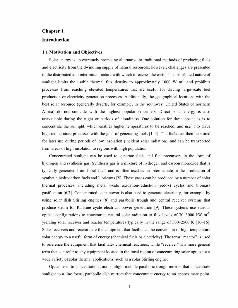
1.1 Motivation and Objectives

Solar energy is an extremely promising alternative to traditional methods of producing fuels

and electricity from the dwindling supply of natural resources; however, challenges are presented

in the distributed and intermittent nature with which it reaches the earth. The distributed nature of

sunlight limits the usable thermal flux density to approximately 1000 W m-2

and prohibits

processes from reaching elevated temperatures that are useful for driving large-scale fuel

production or electricity generation processes. Additionally, the geographical locations with the

best solar resource (generally deserts, for example, in the southwest United States or northern

Africa) do not coincide with the highest population centers. Direct solar energy is also

unavailable during the night or periods of cloudiness. One solution for these obstacles is to

concentrate the sunlight, which enables higher temperatures to be reached, and use it to drive

high-temperature processes with the goal of generating fuels [1–4]. The fuels can then be stored

for later use during periods of low insolation (incident solar radiation), and can be transported

from areas of high insolation to regions with high population.

Concentrated sunlight can be used to generate fuels and fuel precursors in the form of

hydrogen and synthesis gas. Synthesis gas is a mixture of hydrogen and carbon monoxide that is

typically generated from fossil fuels and is often used as an intermediate in the production of

synthetic hydrocarbon fuels and lubricants [5]. These gases can be produced by a number of solar

thermal processes, including metal oxide oxidation-reduction (redox) cycles and biomass

gasification [6,7]. Concentrated solar power is also used to generate electricity, for example by

using solar dish Stirling engines [8] and parabolic trough and central receiver systems that

produce steam for Rankine cycle electrical power generation [9]. These systems use various

optical configurations to concentrate natural solar radiation to flux levels of 70–3000 kW m-2

,

yielding solar receiver and reactor temperatures typically in the range of 500–2500 K [10–16].

Solar receivers and reactors are the equipment that facilitates the conversion of high temperature

solar energy to a useful form of energy (chemical fuels or electricity). The term “reactor” is used

to reference the equipment that facilitates chemical reactions, while “receiver” is a more general

term that can refer to any equipment located in the focal region of concentrating solar optics for a

wide variety of solar thermal applications, such as a solar Stirling engine.

Optics used to concentrate natural sunlight include parabolic trough mirrors that concentrate

sunlight to a line focus, parabolic dish mirrors that concentrate energy to an approximate point,

2

(a) (b) (c)

Fig. 1.1: Schematic drawings of three types of solar concentrating facilities (a) parabolic trough (b) solar dish and (c) central receiver. Images courtesy of Steinfeld & Palumbo [2].

and central receiver facilities that concentrate light to a more distributed point on a larger scale

than a parabolic dish. In all three examples, the receiver type can be altered for the specific

application, and it is located near the region of most intense radiative flux. A common factor in

describing the effectiveness of concentrating optics is the dimensionless concentration ratio, or

the degree to which direct insolation is multiplied after undergoing concentration by various types

of optics. Concentrating optics redirect insolation collected over a large area to a smaller focal

area, thereby increasing the radiative intensity. The concentration ratio is often reported as a

number of suns, where one sun corresponds to 1000 W m-2

[2]. Greater flux levels are considered

to be concentrated. For a region with constant incident radiative flux ,q the blackbody

stagnation temperature Tb is calculated by the Stefan-Boltzmann law:

qT 4b (1.1)

where is the Stefan-Boltzmann constant. It is the maximum theoretical temperature that an ideal

blackbody could reach with zero losses. Schematic drawings of the three types of systems are

shown in Fig. 1.1, and further details regarding the use of these facilities follow.

Parabolic trough facilities consist of a linear mirror with a parabolic cross-section, as seen in

Fig. 1.1a, which tracks the sun’s altitude throughout the day. A fluid is passed through a tube

along the linear focus and transferred to the necessary application (e.g. steam for power plants or

oil as a heat transfer medium). An example of such a facility is the series of Solar Energy

Generating Systems (SEGS) that comprise steam Rankine power plants located in California.

Two of these plants (SEGS VIII and IX, located in Harper Lake, CA) each produce up to 80 MWe

by using solar-heated steam, rather than using steam supplied by a conventional boiler (e.g., coal

or natural gas). A heat transfer fluid (in this case, oil) is flowed through the receiver tubes, and its

sensible energy is transferred to water through a series of heat exchangers to generate high-

pressure steam (100bar, 370°C), [17]. These parabolic trough collectors have an aperture width of

3

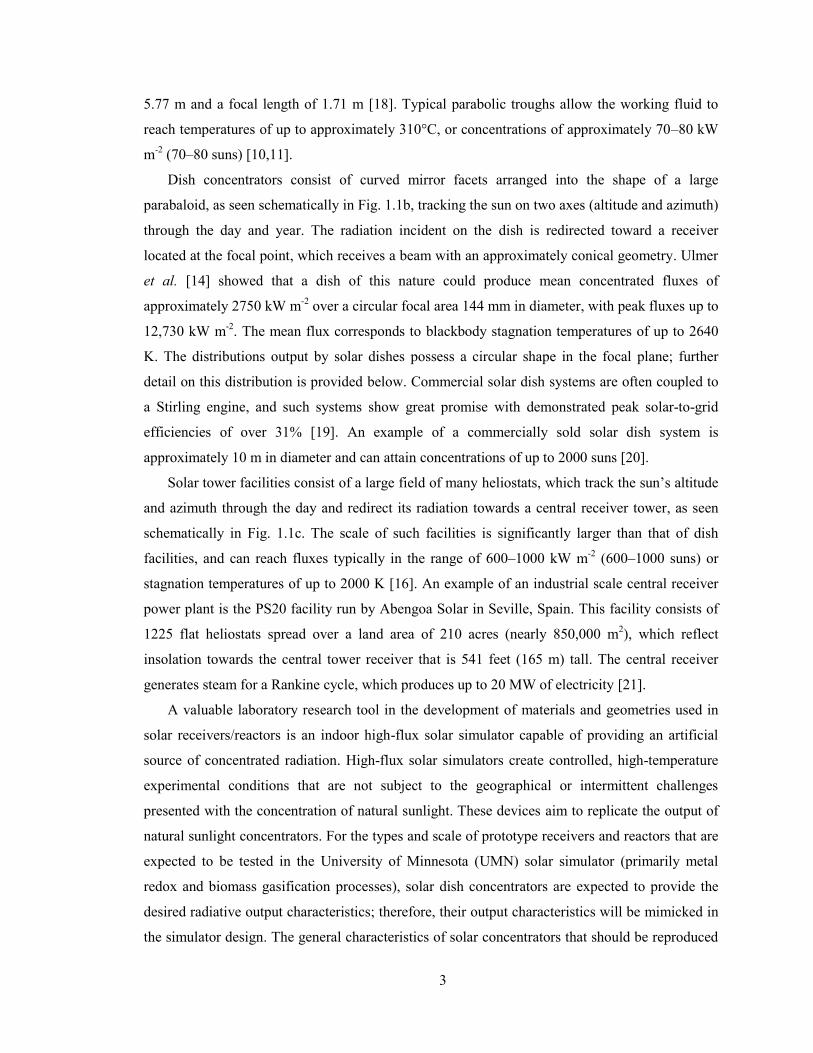
5.77 m and a focal length of 1.71 m [18]. Typical parabolic troughs allow the working fluid to

reach temperatures of up to approximately 310°C, or concentrations of approximately 70–80 kW

m-2

(70–80 suns) [10,11].

Dish concentrators consist of curved mirror facets arranged into the shape of a large

parabaloid, as seen schematically in Fig. 1.1b, tracking the sun on two axes (altitude and azimuth)

through the day and year. The radiation incident on the dish is redirected toward a receiver

located at the focal point, which receives a beam with an approximately conical geometry. Ulmer

et al. [14] showed that a dish of this nature could produce mean concentrated fluxes of

approximately 2750 kW m-2

over a circular focal area 144 mm in diameter, with peak fluxes up to

12,730 kW m-2

. The mean flux corresponds to blackbody stagnation temperatures of up to 2640

K. The distributions output by solar dishes possess a circular shape in the focal plane; further

detail on this distribution is provided below. Commercial solar dish systems are often coupled to

a Stirling engine, and such systems show great promise with demonstrated peak solar-to-grid

efficiencies of over 31% [19]. An example of a commercially sold solar dish system is

approximately 10 m in diameter and can attain concentrations of up to 2000 suns [20].

Solar tower facilities consist of a large field of many heliostats, which track the sun’s altitude

and azimuth through the day and redirect its radiation towards a central receiver tower, as seen

schematically in Fig. 1.1c. The scale of such facilities is significantly larger than that of dish

facilities, and can reach fluxes typically in the range of 600–1000 kW m-2

(600–1000 suns) or

stagnation temperatures of up to 2000 K [16]. An example of an industrial scale central receiver

power plant is the PS20 facility run by Abengoa Solar in Seville, Spain. This facility consists of

1225 flat heliostats spread over a land area of 210 acres (nearly 850,000 m2), which reflect

insolation towards the central tower receiver that is 541 feet (165 m) tall. The central receiver

generates steam for a Rankine cycle, which produces up to 20 MW of electricity [21].

A valuable laboratory research tool in the development of materials and geometries used in

solar receivers/reactors is an indoor high-flux solar simulator capable of providing an artificial

source of concentrated radiation. High-flux solar simulators create controlled, high-temperature

experimental conditions that are not subject to the geographical or intermittent challenges

presented with the concentration of natural sunlight. These devices aim to replicate the output of

natural sunlight concentrators. For the types and scale of prototype receivers and reactors that are

expected to be tested in the University of Minnesota (UMN) solar simulator (primarily metal

redox and biomass gasification processes), solar dish concentrators are expected to provide the

desired radiative output characteristics; therefore, their output characteristics will be mimicked in

the simulator design. The general characteristics of solar concentrators that should be reproduced

4

include the beam geometry, the irradiated area, the relative distribution of the flux, and the solar

spectral distribution. The beam geometry is defined by the cone that confines the radiation

incident on the focal plane; the relative distribution of flux is quantified by the peak-to-mean flux

ratio S; the averaged solar spectral distribution is quantified by the air mass (AM) 1.5 spectrum

[22].

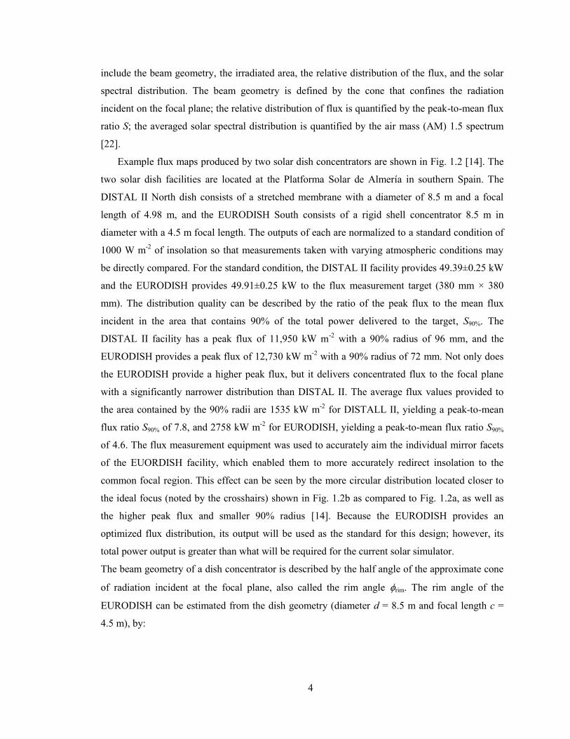
Example flux maps produced by two solar dish concentrators are shown in Fig. 1.2 [14]. The

two solar dish facilities are located at the Platforma Solar de Almería in southern Spain. The

DISTAL II North dish consists of a stretched membrane with a diameter of 8.5 m and a focal

length of 4.98 m, and the EURODISH South consists of a rigid shell concentrator 8.5 m in

diameter with a 4.5 m focal length. The outputs of each are normalized to a standard condition of

1000 W m-2

of insolation so that measurements taken with varying atmospheric conditions may

be directly compared. For the standard condition, the DISTAL II facility provides 49.39±0.25 kW

and the EURODISH provides 49.91±0.25 kW to the flux measurement target (380 mm × 380

mm). The distribution quality can be described by the ratio of the peak flux to the mean flux

incident in the area that contains 90% of the total power delivered to the target, S90%. The

DISTAL II facility has a peak flux of 11,950 kW m-2

with a 90% radius of 96 mm, and the

EURODISH provides a peak flux of 12,730 kW m-2

with a 90% radius of 72 mm. Not only does

the EURODISH provide a higher peak flux, but it delivers concentrated flux to the focal plane

with a significantly narrower distribution than DISTAL II. The average flux values provided to

the area contained by the 90% radii are 1535 kW m-2

for DISTALL II, yielding a peak-to-mean

flux ratio S90% of 7.8, and 2758 kW m-2

for EURODISH, yielding a peak-to-mean flux ratio S90%

of 4.6. The flux measurement equipment was used to accurately aim the individual mirror facets

of the EUORDISH facility, which enabled them to more accurately redirect insolation to the

common focal region. This effect can be seen by the more circular distribution located closer to

the ideal focus (noted by the crosshairs) shown in Fig. 1.2b as compared to Fig. 1.2a, as well as

the higher peak flux and smaller 90% radius [14]. Because the EURODISH provides an

optimized flux distribution, its output will be used as the standard for this design; however, its

total power output is greater than what will be required for the current solar simulator.

The beam geometry of a dish concentrator is described by the half angle of the approximate cone

of radiation incident at the focal plane, also called the rim angle rim. The rim angle of the

EURODISH can be estimated from the dish geometry (diameter d = 8.5 m and focal length c =

4.5 m), by:

5

(a)

(b)

Fig. 1.2: Sample flux distributions taken in the focal planes of two different solar dish concentrators (a) DISTAL II North and (b) EURODISH South. The crosshairs represent the center of the ideally-focused concentrator and the flux levels are displayed on a logarithmic scale after being normalized to a standard insolation of 1000 W m

-2 [23]

6

2

16tan

2

1rim d

cdc

(1.2)

The published parameters result in a rim angle of approximately 39.4°. This rim angle, ±5°, will

be the approximate goal in designing the geometry of the UMN solar simulator. Additionally, the

order of magnitude of the irradiated area provided by the EURODISH (tens of millimeters) is

representative of the desired irradiated area for the UMN solar simulator.

Some options for artificially providing this radiative output include (a) using high-powered

lasers individually or in groups to achieve the necessary spectrum and geometry, as well as the

required power and concentration [24], (b) redirecting the radiation output of artificial sources as

high-flux radiation with a uniform distribution to the test area [25,26], or (c) coupling an artificial

radiation source in the form of a high intensity discharge or arc lamp to an appropriately-designed

reflector [27–33]. The benefits and challenges associated with each of these options are described

below.

Solar simulation using lasers allows for rapid and controlled heating of material samples with

power and concentration levels that approach those presented by concentrated natural sunlight.

Beattie successfully provided flux levels up to 2500 kW m-2

to a small area of approximately 1

mm2 using a CO2 laser at a wavelength of 10.6 m [24]. Although the laser provided a radiative

flux whose magnitude reasonably replicated that of concentrated sunlight, the beam geometry,

spectral distribution, and irradiated area did not accurately imitate the conditions presented by

natural solar concentrators due to the laser’s narrow beam and single wavelength. The inaccurate

spectral representation could be remedied by superposing the outputs of many lasers with varying

intensity and spectral bands. Additionally, the grouping could also be arranged such that an

approximate cone of radiation is generated and a larger area is irradiated; however, it is expected

that the cost associated with the number of high-powered lasers required to fully replicate the

conditions generated by a concentrator of natural sunlight would be prohibitively high.

Another method that can be used to provide high-flux radiative power to laboratory-scale

prototype receivers and reactors is to use a series of reflectors and lenses to collimate the

radiation output by an array of artificial radiation sources and redirect it towards the prototype, as

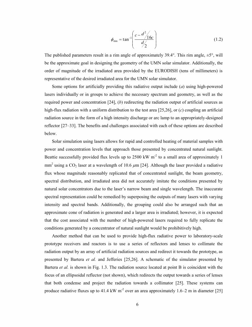
presented by Bartera et al. and Jefferies [25,26]. A schematic of the simulator presented by

Bartera et al. is shown in Fig. 1.3. The radiation source located at point B is coincident with the

focus of an ellipsoidal reflector (not shown), which redirects the output towards a series of lenses

that both condense and project the radiation towards a collimator [25]. These systems can

produce radiative fluxes up to 41.4 kW m-2

over an area approximately 1.6–2 m in diameter [25]

7

Fig. 1.3: Schematic of the solar simulator at the Jet Propulsion Laboratory [25]

or up to 1.8 kW m-2

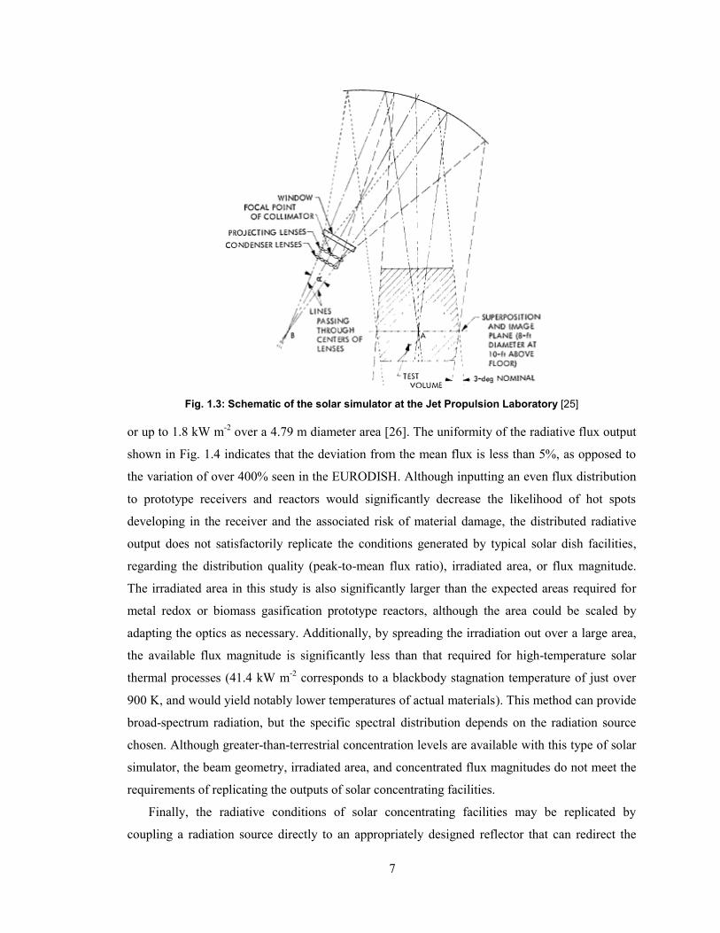
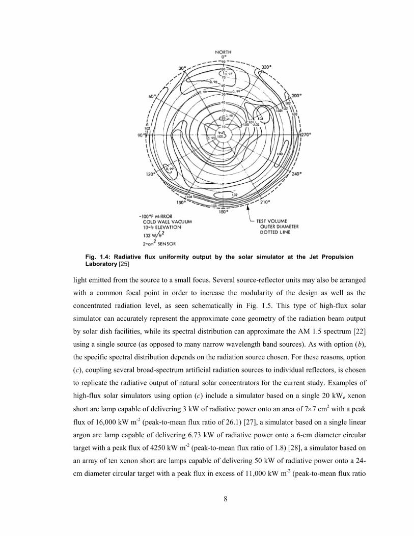
over a 4.79 m diameter area [26]. The uniformity of the radiative flux output

shown in Fig. 1.4 indicates that the deviation from the mean flux is less than 5%, as opposed to

the variation of over 400% seen in the EURODISH. Although inputting an even flux distribution

to prototype receivers and reactors would significantly decrease the likelihood of hot spots

developing in the receiver and the associated risk of material damage, the distributed radiative

output does not satisfactorily replicate the conditions generated by typical solar dish facilities,

regarding the distribution quality (peak-to-mean flux ratio), irradiated area, or flux magnitude.

The irradiated area in this study is also significantly larger than the expected areas required for

metal redox or biomass gasification prototype reactors, although the area could be scaled by

adapting the optics as necessary. Additionally, by spreading the irradiation out over a large area,

the available flux magnitude is significantly less than that required for high-temperature solar

thermal processes (41.4 kW m-2

corresponds to a blackbody stagnation temperature of just over

900 K, and would yield notably lower temperatures of actual materials). This method can provide

broad-spectrum radiation, but the specific spectral distribution depends on the radiation source

chosen. Although greater-than-terrestrial concentration levels are available with this type of solar

simulator, the beam geometry, irradiated area, and concentrated flux magnitudes do not meet the

requirements of replicating the outputs of solar concentrating facilities.

Finally, the radiative conditions of solar concentrating facilities may be replicated by

coupling a radiation source directly to an appropriately designed reflector that can redirect the

8

Fig. 1.4: Radiative flux uniformity output by the solar simulator at the Jet Propulsion Laboratory [25]

light emitted from the source to a small focus. Several source-reflector units may also be arranged

with a common focal point in order to increase the modularity of the design as well as the

concentrated radiation level, as seen schematically in Fig. 1.5. This type of high-flux solar

simulator can accurately represent the approximate cone geometry of the radiation beam output

by solar dish facilities, while its spectral distribution can approximate the AM 1.5 spectrum [22]

using a single source (as opposed to many narrow wavelength band sources). As with option (b),

the specific spectral distribution depends on the radiation source chosen. For these reasons, option

(c), coupling several broad-spectrum artificial radiation sources to individual reflectors, is chosen

to replicate the radiative output of natural solar concentrators for the current study. Examples of

high-flux solar simulators using option (c) include a simulator based on a single 20 kWe xenon

short arc lamp capable of delivering 3 kW of radiative power onto an area of 77 cm2 with a peak

flux of 16,000 kW m-2

(peak-to-mean flux ratio of 26.1) [27], a simulator based on a single linear

argon arc lamp capable of delivering 6.73 kW of radiative power onto a 6-cm diameter circular

target with a peak flux of 4250 kW m-2

(peak-to-mean flux ratio of 1.8) [28], a simulator based on

an array of ten xenon short arc lamps capable of delivering 50 kW of radiative power onto a 24-

cm diameter circular target with a peak flux in excess of 11,000 kW m-2

(peak-to-mean flux ratio

9

of 10.0) [29], a similar simulator based on an array of ten xenon arc lamps that can deliver 20

kWth to a target area of approximately 100 cm² with a peak irradiance greater than 4100 kW m-²

(peak-to-mean flux ratio of 2.1) [30], an array of seven xenon arc lamps that can deliver radiant

fluxes of up to 5000 kW m-2

[31,34], and the recently installed simulator at the UMN that is

described in this study, capable of delivering 9.2 kW over a 60-mm diameter circular area located

in the focal plane, corresponding to an average flux of 3200 kW m-2

, with a peak flux of 7300 kW

m-2

(peak-to-mean flux ratio of 2.2) [32,33].

Designing a solar simulator by coupling a single radiation source to an ellipsoidal reflector

requires the precise selection and location of the reflector geometry relative to the source and

target points [27,28]. When the solar simulator design is expanded to incorporate a series of

radiation sources, each coupled to a precision reflector and all having a common focus [29,32],

the design is complicated by requiring that the target focal points of all reflectors coincide.

Petrasch et al. [29] addressed the challenge of coinciding the foci of ten lamp-reflector modules

for the specific facility studied, but the design presented does not allow for generalized use. As

part of this work, a set of generalized equations has been developed to ensure a common focal

point of the individual reflectors. These equations provide a design framework that allows for the

flexibility to apply factors that are specific to the particular facility. Such factors include the

physical space available, the desired geometry of the resulting beam of radiation, required

experimental access space, manufacturer recommendations for the radiation source operating

conditions, and manufacturability of the individual components.

Solar thermochemical

reactor

rim

6.5 kW xenon

arc lamp

Ellipsoidal

reflector

Fig. 1.5: Conceptual drawing of a concentrating solar simulator using a series of lamps and ellipsoidal reflectors

10

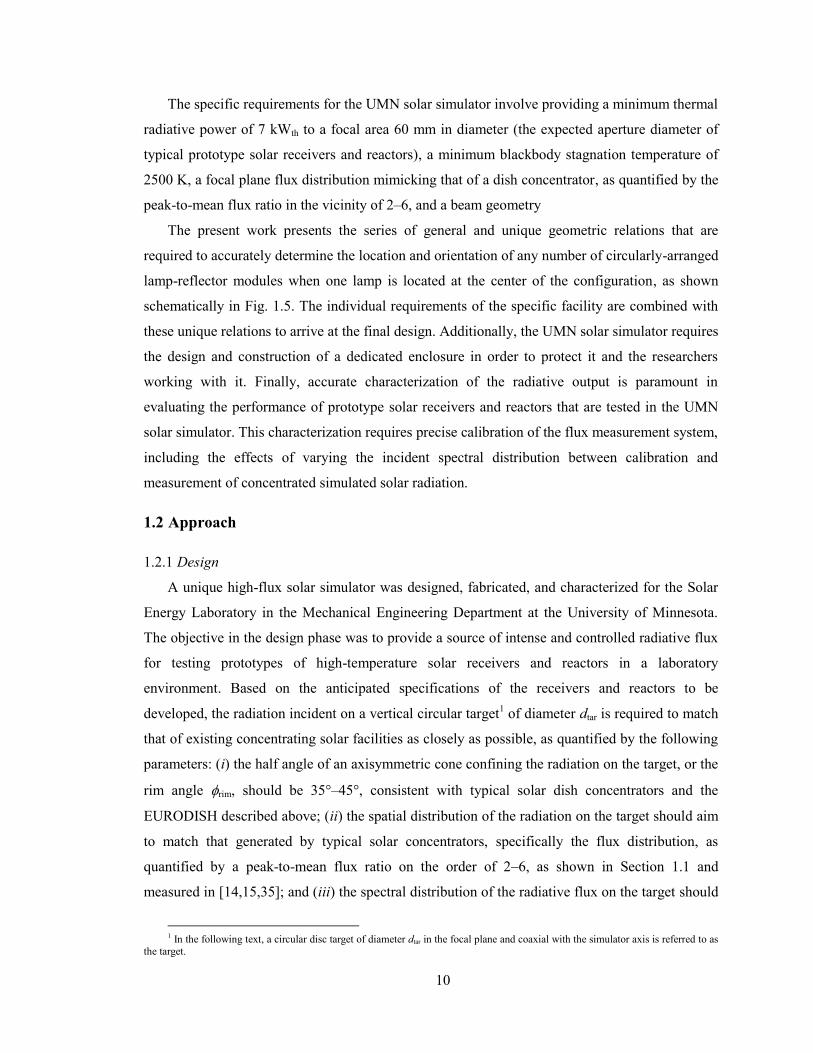
The specific requirements for the UMN solar simulator involve providing a minimum thermal

radiative power of 7 kWth to a focal area 60 mm in diameter (the expected aperture diameter of

typical prototype solar receivers and reactors), a minimum blackbody stagnation temperature of

2500 K, a focal plane flux distribution mimicking that of a dish concentrator, as quantified by the

peak-to-mean flux ratio in the vicinity of 2–6, and a beam geometry

The present work presents the series of general and unique geometric relations that are

required to accurately determine the location and orientation of any number of circularly-arranged

lamp-reflector modules when one lamp is located at the center of the configuration, as shown

schematically in Fig. 1.5. The individual requirements of the specific facility are combined with

these unique relations to arrive at the final design. Additionally, the UMN solar simulator requires

the design and construction of a dedicated enclosure in order to protect it and the researchers

working with it. Finally, accurate characterization of the radiative output is paramount in

evaluating the performance of prototype solar receivers and reactors that are tested in the UMN

solar simulator. This characterization requires precise calibration of the flux measurement system,

including the effects of varying the incident spectral distribution between calibration and

measurement of concentrated simulated solar radiation.

1.2 Approach

1.2.1 Design

A unique high-flux solar simulator was designed, fabricated, and characterized for the Solar

Energy Laboratory in the Mechanical Engineering Department at the University of Minnesota.

The objective in the design phase was to provide a source of intense and controlled radiative flux

for testing prototypes of high-temperature solar receivers and reactors in a laboratory

environment. Based on the anticipated specifications of the receivers and reactors to be

developed, the radiation incident on a vertical circular target1 of diameter dtar is required to match

that of existing concentrating solar facilities as closely as possible, as quantified by the following

parameters: (i) the half angle of an axisymmetric cone confining the radiation on the target, or the

rim angle rim, should be 35°–45°, consistent with typical solar dish concentrators and the

EURODISH described above; (ii) the spatial distribution of the radiation on the target should aim

to match that generated by typical solar concentrators, specifically the flux distribution, as

quantified by a peak-to-mean flux ratio on the order of 2–6, as shown in Section 1.1 and

measured in [14,15,35]; and (iii) the spectral distribution of the radiative flux on the target should

1 In the following text, a circular disc target of diameter dtar in the focal plane and coaxial with the simulator axis is referred to as

the target.

11

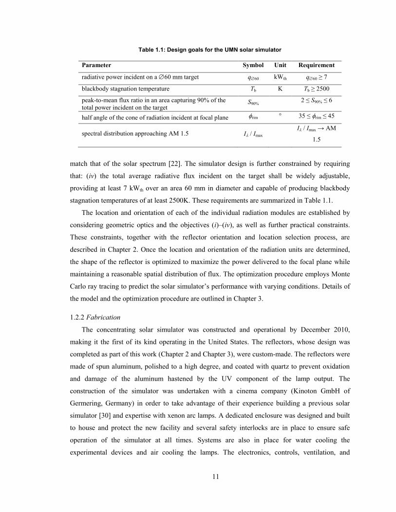
Table 1.1: Design goals for the UMN solar simulator

Parameter Symbol Unit Requirement

radiative power incident on a 60 mm target q60 kWth q60 ≥ 7

blackbody stagnation temperature Tb K Tb ≥ 2500

peak-to-mean flux ratio in an area capturing 90% of the

total power incident on the target S90% 2 ≤ S90% ≤ 6

half angle of the cone of radiation incident at focal plane rim ° 35 ≤ rim ≤ 45

spectral distribution approaching AM 1.5 I / Imax I / Imax → AM

1.5

match that of the solar spectrum [22]. The simulator design is further constrained by requiring

that: (iv) the total average radiative flux incident on the target shall be widely adjustable,

providing at least 7 kWth over an area 60 mm in diameter and capable of producing blackbody

stagnation temperatures of at least 2500K. These requirements are summarized in Table 1.1.

The location and orientation of each of the individual radiation modules are established by

considering geometric optics and the objectives (i)–(iv), as well as further practical constraints.

These constraints, together with the reflector orientation and location selection process, are

described in Chapter 2. Once the location and orientation of the radiation units are determined,

the shape of the reflector is optimized to maximize the power delivered to the focal plane while

maintaining a reasonable spatial distribution of flux. The optimization procedure employs Monte

Carlo ray tracing to predict the solar simulator’s performance with varying conditions. Details of

the model and the optimization procedure are outlined in Chapter 3.

1.2.2 Fabrication

The concentrating solar simulator was constructed and operational by December 2010,

making it the first of its kind operating in the United States. The reflectors, whose design was

completed as part of this work (Chapter 2 and Chapter 3), were custom-made. The reflectors were

made of spun aluminum, polished to a high degree, and coated with quartz to prevent oxidation

and damage of the aluminum hastened by the UV component of the lamp output. The

construction of the simulator was undertaken with a cinema company (Kinoton GmbH of

Germering, Germany) in order to take advantage of their experience building a previous solar

simulator [30] and expertise with xenon arc lamps. A dedicated enclosure was designed and built

to house and protect the new facility and several safety interlocks are in place to ensure safe

operation of the simulator at all times. Systems are also in place for water cooling the

experimental devices and air cooling the lamps. The electronics, controls, ventilation, and

12

dedicated enclosure were developed in collaboration with Kinoton and local engineers, architects,

and contractors. Details of the completed facility can be found in Chapter 4.

1.2.3 Characterization

Accurate knowledge of the solar simulator’s radiative output is a critical element in the

meaningful evaluation of the performance of prototype receivers and reactors, particularly in

determining their efficiency and other benchmark standards. Analysis of these prototypes’

behavior requires knowledge of both the distribution and quantity of radiative flux and power

incident in the focal plane. Because these values constitute the energy input in calculating thermal

process efficiency, their accuracy is paramount. An uncertainty in flux and power measurements

of ±3% or less is expected for these results. Reported fluxes produced by solar dish facilities have

uncertainty values of approximately ±2–4% [14], which indicate that the goal of ±3% is

attainable. Additionally, if a receiver or reactor efficiency was calculated with this radiative

power input as the denominator, the ±3% uncertainty in cumulative radiative power would

correspond to an acceptable uncertainty in the efficiency of ±3%, not accounting for any

uncertainty in the nominator of the efficiency. Further details of the flux measurement methods

are found in Chapter 5.

Direct flux distribution measurement can be achieved in two dimensions with one of the

following methods: (a) a series or array of heat flux gages, calorimeters, or radiometers is located

in the measurement plane, discretely measuring the two-dimensional distribution, (b) a single

sensor is transversed across the area of interest, or (c) a water calorimeter is located in the

measurement plane and measures the absorbed energy with varying aperture sizes to obtain a

distribution. The resulting spatial resolution would be limited by the size of the sensor apertures

for all cases, with additional contributions by the number of sensors used and their spacing for

case (a) and the accuracy of the transversing mechanism for case (b). Additionally, possible

temporal changes in the radiative output of the solar simulator could only be captured by method

(a), and would affect the quality of the two-dimensional flux distributions measured by methods

(b) and (c).

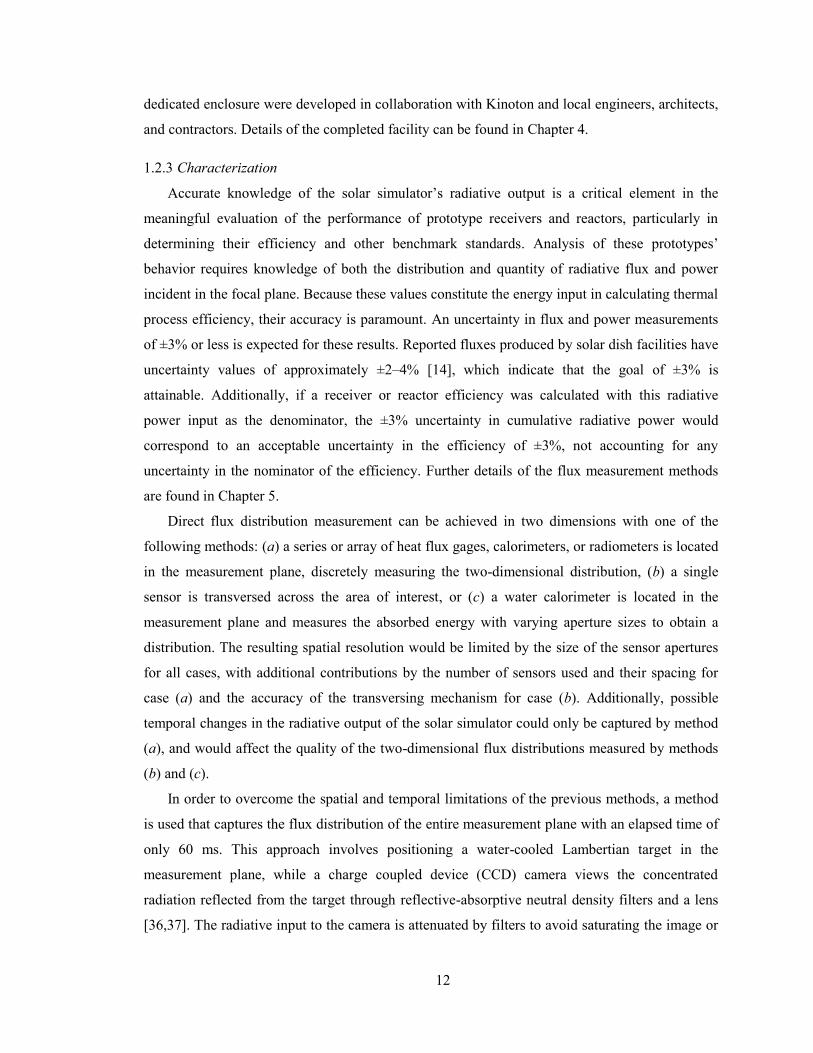
In order to overcome the spatial and temporal limitations of the previous methods, a method

is used that captures the flux distribution of the entire measurement plane with an elapsed time of

only 60 ms. This approach involves positioning a water-cooled Lambertian target in the

measurement plane, while a charge coupled device (CCD) camera views the concentrated

radiation reflected from the target through reflective-absorptive neutral density filters and a lens

[36,37]. The radiative input to the camera is attenuated by filters to avoid saturating the image or

13

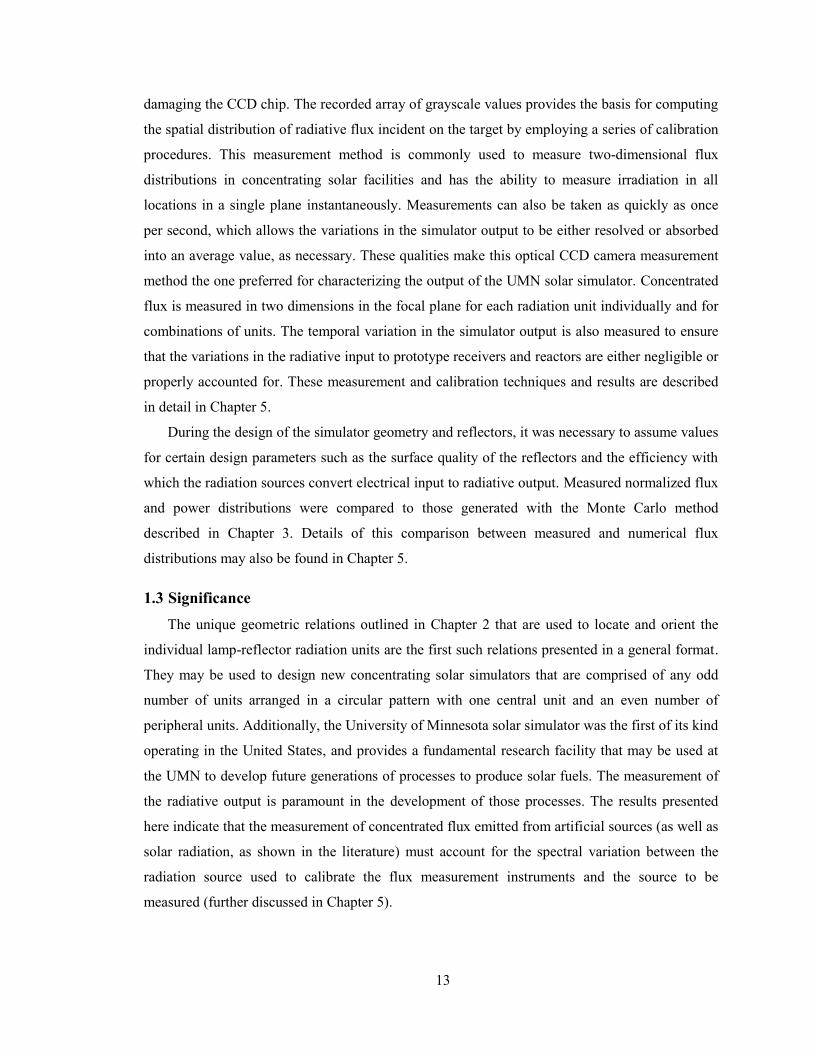
damaging the CCD chip. The recorded array of grayscale values provides the basis for computing

the spatial distribution of radiative flux incident on the target by employing a series of calibration

procedures. This measurement method is commonly used to measure two-dimensional flux

distributions in concentrating solar facilities and has the ability to measure irradiation in all

locations in a single plane instantaneously. Measurements can also be taken as quickly as once

per second, which allows the variations in the simulator output to be either resolved or absorbed

into an average value, as necessary. These qualities make this optical CCD camera measurement

method the one preferred for characterizing the output of the UMN solar simulator. Concentrated

flux is measured in two dimensions in the focal plane for each radiation unit individually and for

combinations of units. The temporal variation in the simulator output is also measured to ensure

that the variations in the radiative input to prototype receivers and reactors are either negligible or

properly accounted for. These measurement and calibration techniques and results are described

in detail in Chapter 5.

During the design of the simulator geometry and reflectors, it was necessary to assume values

for certain design parameters such as the surface quality of the reflectors and the efficiency with

which the radiation sources convert electrical input to radiative output. Measured normalized flux

and power distributions were compared to those generated with the Monte Carlo method

described in Chapter 3. Details of this comparison between measured and numerical flux

distributions may also be found in Chapter 5.

1.3 Significance

The unique geometric relations outlined in Chapter 2 that are used to locate and orient the

individual lamp-reflector radiation units are the first such relations presented in a general format.

They may be used to design new concentrating solar simulators that are comprised of any odd

number of units arranged in a circular pattern with one central unit and an even number of

peripheral units. Additionally, the University of Minnesota solar simulator was the first of its kind

operating in the United States, and provides a fundamental research facility that may be used at

the UMN to develop future generations of processes to produce solar fuels. The measurement of

the radiative output is paramount in the development of those processes. The results presented

here indicate that the measurement of concentrated flux emitted from artificial sources (as well as

solar radiation, as shown in the literature) must account for the spectral variation between the

radiation source used to calibrate the flux measurement instruments and the source to be

measured (further discussed in Chapter 5).

14

Chapter 2

Solar Simulator Design

The primary goal in designing the UMN solar simulator is to achieve at least 7 kWth over a 6

cm diameter focal area and a blackbody stagnation temperature of at least 2500 K, while

mimicking the spectral and spatial distributions of the conditions generated by solar dish

facilities. The spatial conditions were outlined in Section 1.1, and the spectral conditions are

described in further detail below. The concentrating optics are designed by considering the

geometric optical properties of the ellipsoidal reflectors and practical design requirements, such

as manufacturability of the reflectors and constraints imposed on the total solar simulator size by

the room in which it is housed. The location and orientation of each lamp-reflector unit is

determined by requiring that the energy output by each is focused to a common area.

Unique geometric relations are developed that relate all geometric variables specifying the

location and orientation of the lamp-reflector units to four independent parameters (see Fig. 2.1

and Fig. 2.2): the projected orientation angle of each unit with respect to the horizontal plane

crossing through the central unit i, the diameter of an individual reflector d, the minimum

distance between the focal plane and the nearest point of a radiation module l1, and the angle

between the axis of the central module and the axis of any peripheral module . The final

combination of these parameters is chosen with the goals of obtaining a rim angle rim—defined

as the half-angle of the cone of light incident at the focal plane—maximized in the range of 35°–

45°, minimizing the tilt angle of all lamp axes with respect to the horizontal plane, and

Fig. 2.1: Schematic of the array of lamp-reflector modules: (a) front view showing the seven lamp/reflector assemblies and (b) center cross-section through the line in (a) depicting the relationship to a prototype receiver/reactor

(b) (a)

15

Fig. 2.2: Schematic of the inner surface of a single reflector (bold outline) with respect to a full ellipse (thin outline)

maintaining at least 50 mm between the inner reflector surfaces to allow for clamping and

mounting.

2.1 Lamp Selection and Spectral Considerations

One goal in developing the solar simulator is to match its spectral output distribution to that

of the air mass 1.5 spectrum (AM 1.5) [22], but a perfect match is not possible with artificial

radiation sources. While spectral filters may be applied to low-flux solar simulators, which are

commonly used to test flat-plate collectors, photovoltaic cells, and photo-chemical and photo-

biological processes [38–40], the application of such filters at high flux levels is not trivial. For

example, if filters are to be applied directly to the radiation source (e.g., using the materials in

[41]), the elevated absorptivity over the envelope would lead to higher temperatures and thermal

stresses of the delicate quartz structure, and may cause serious damage. The use of water sheets

between glass panes (e.g., in [40]) at the large scales required in this study introduces the risk of

flooding, which would be extremely dangerous in the vicinity of the high electrical power

required to run the solar simulator (further detail in Chapter 4). Additionally, the water achieves

filtration by absorption, and at the elevated flux levels produced by the solar simulator, it is

possible that the water may reach elevated temperatures consistent with boiling. The application

of optical filters would also decrease the amount of radiative energy available to the prototype

receivers and reactors; Seckmeyer et al. estimated an efficiency of less than 2% for a low-flux

solar simulator using xenon arc lamps as the radiation source with absorbing and reflecting glass

applied as spectral filters. In this study, the desired spectral response is obtained by the choice of

radiation source.

The primary considerations in choosing radiation sources are the degree to which the spectral

distribution approximates sunlight and the physical size of the source. If the radiative properties

of the materials used in prototype receivers and reactors have a strong spectral dependence (for

16

Fig. 2.3: Spectral emission distributions of the xenon arc lamp chosen for this application (gray line with markers), the HMI® 6000W/SE metal halide lamp [42], and Air Mass 1.5 (red, solid line) [22]

example, in absorptivity), the differences in the spectra could alter the behavior of the prototype

from testing in the solar simulator to further use in concentrated natural sunlight. This effect is

limited by choosing a radiation source with good spectral characteristics and would be most

pronounced in materials with widely varying spectral properties. Additionally, because lamps do

not emit from a point, the physical arc size is an important consideration in their performance

when coupled with concentrating optics. The geometry of an ellipsoidal reflector, for example,

focuses light emitted from one focal point to the other focus. The distance between the light’s

arrival point and the ideal target focus is directly correlated with the distance between the

emission point and the ideal source focal point. When a ray is launched farther from the ideal

source, it arrives farther away from the ideal target point, which decreases the maximum available

concentration near the target point. Steinfeld [43] similarly found that a smaller arc allows the

reflector to more effectively redirect radiation towards the target focus. Examples of radiation

sources considered include the Osram HMI® 6000 W/SE metal halide lamp, which has an

electrode gap of 23 mm [44], and the Osram XBO® 6500W/HSLA OFR and XBO® 7000W/HS

XL OFR xenon short arc lamps, which have electrode gaps of 7.5 and 11 mm, respectively [42].

The arc length is related to the size of the cold electrode gap in high-intensity discharge lamps,

but the effective arc length is somewhat smaller than the electrode gap in both instances due to

the thermal expansion of the electrodes during operation.

0 500 1000 1500 20000

0.5

1.0

1.5

2.0

2.5

(nm)

No

rma

lize

d S

pe

ctr

al In

ten

sity I

/ I,m

ax

AM 1.5

XBO 6500W/HSLA

HMI 6000W/SE

17

Normalized emission spectra of AM 1.5, the Osram XBO® 6500W/HSLA xenon arc lamp,

and the Osram HMI® 6000 W/SE metal halide lamp are depicted in Fig. 2.3. By integrating each

normalized spectrum and comparing each artificial source to the AM 1.5 distribution, it is

determined that the xenon arc lamp emits approximately 49% more energy and the metal halide

emits 36% less energy than AM 1.5 in the wavelength range of 280–500 nm. In the wavelength

range of 700–1100 nm, the xenon arc lamp emits approximately 76% more energy and the metal

halide lamp emits approximately 42% less energy than the AM 1.5 distribution. Neither artificial

source’s emission spectrum perfectly replicates AM 1.5, but the deviations between AM 1.5 and

the metal halide lamp are smaller than the deviations for the xenon arc lamp.

Based on the spectral distributions alone, neither source perfectly matches AM 1.5. The

deciding factor in choosing a radiation source becomes the arc size. The metal halide lamp’s

significantly larger arc size (23 mm) corresponds to a 60% decrease in radiative power delivered

to a 60-mm diameter target as compared to the 7.5 mm arc length, as calculated for a single lamp

with constant reflector geometry using the methods outlined in Chapter 3. The XBO®

6500W/HSLA OFR OSRAM lamp has been chosen for this application because it provides the

smallest arc size available for its emitted power with an acceptable spectral distribution match.

Seven modules are chosen for this application in order to meet both aspects of condition (iv),

outlined in Chapter 1, requiring an output power of at least 7 kWth in a 6 cm diameter focal area

that may be tuned to lower levels as necessary. The total radiative power output by the simulator

is adjustable by turning individual lamps on and off as necessary. Seven lamps are determined to

meet the delivered thermal power goal by the following preliminary calculation: An example case

of the solar simulator at the Paul Scherrer Institut was able to deliver approximately 20 kWth to a

60 mm diameter focal area, q60, when the total input electrical input, Nlamps Iarc Varc, was equal to

150 kWe [29]. From these values, a delivery efficiency 60 of 13% was calculated by:

.kW15lamps10

kW20

e

th

arcarclamps

60

60

VIN

q

(2.1)

The bulbs used in that particular study had a 29% conversion efficiency from electrical input to

radiative output in the arc in the wavelength range of 250-800 nm [29]; however, the radiative

power goals set forth in designing the current simulator also account for the energy emitted in

longer wavelengths. Using the provided spectral data for the OSRAM XBO® 6500W/HSLA

OFR lamps used in this study, an electrical-to-radiation conversion efficiency of 69%, as

calculated by integrating the spectral energy λq output in the wavelength range of 250–1650 nm

[29,42]:

18

arcarc

re

d

VI

qλ

(2.2)

Therefore, the 13% delivery efficiency demonstrated by Petrasch et al. is increased by a factor of

2.4 to account for the different arc characteristics and applicable wavelength ranges, resulting in a

predicted delivery efficiency of 32%. When this value is applied to the case of seven 6.5 kW

xenon arc lamps in Eq. (2.1), the predicted delivered radiative power is 14.4 kWth. This

preliminary calculation indicates that this combination of bulbs may be combined with

appropriately designed reflectors to achieve the required 7 kWth with a safety factor of 2.1. The

safety factor is included, rather than decreasing the number of radiation units used, to account for

instances when the lamps are operated at less than full input power, variations in reflector

effectiveness, and the possibility of an inaccurate spectral distribution. It should be noted that a

more conservative value of e-r=50% is used in Chapter 3 to add an additional factor of safety

into the design. As shown in Chapter 5, the chosen combination of lamps provides approximately

9.2 kWth to a 60 mm diameter focal area, with a delivery efficiency of 25%.

In order to concentrate the light emitted by the artificial radiation sources, the lamp arcs are

located at one focal point of a reflector in the shape of a truncated ellipsoid of revolution, as

shown in Fig. 2.2. Rays originating from a point source can be collected in their entirety on a

target point by placing the source and target points on the foci of an ideal ellipsoid of revolution

with specularly reflecting walls. In real systems, non-idealities such as finite dimensions of real

radiative sources and specular reflection imperfections at real surfaces result in radiation that does

not intersect the target point. Radiative exchange between two spheres placed at the foci of a

specularly-reflecting ellipsoidal cavity is analyzed by Steinfeld [43]. It is shown that the

efficiency of energy transferred from the spherical source located at one focal point to a spherical

target centered at the other focal point increases when the eccentricity of the ellipsoid and the size

of the diffuse spherical source decrease.

One design would be based on a single ellipsoidal mirror with a small, high-intensity source

of diffuse radiation. This concept was previously used by Guesdon et al. [45]; however, the

resulting single large ellipsoidal mirror and a limited ability to adjust the source power resulted in

a relatively narrow range of power output. A range of approximately 4–15 MWm2 was achieved

simply by moving the sample in and out of the focal plane. To overcome these disadvantages and

better meet requirement (iv), the current design builds on the approach of Petrasch et al., which

used an array of commonly focused radiation units, each comprised of a truncated ellipsoidal

reflector close-coupled to a short arc lamp [29].

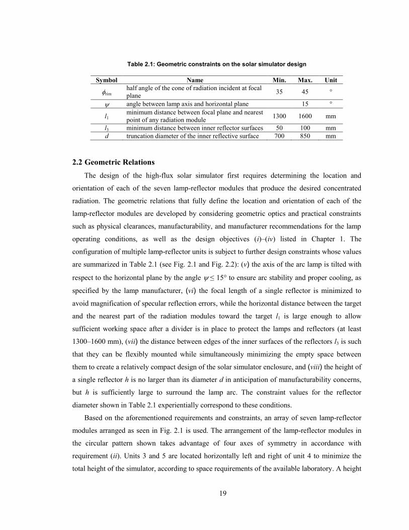
19

Table 2.1: Geometric constraints on the solar simulator design

Symbol Name Min. Max. Unit

rim half angle of the cone of radiation incident at focal

plane 35 45 °

angle between lamp axis and horizontal plane 15 °

l1 minimum distance between focal plane and nearest

point of any radiation module 1300 1600 mm

l3 minimum distance between inner reflector surfaces 50 100 mm

d truncation diameter of the inner reflective surface 700 850 mm

2.2 Geometric Relations

The design of the high-flux solar simulator first requires determining the location and

orientation of each of the seven lamp-reflector modules that produce the desired concentrated

radiation. The geometric relations that fully define the location and orientation of each of the

lamp-reflector modules are developed by considering geometric optics and practical constraints

such as physical clearances, manufacturability, and manufacturer recommendations for the lamp

operating conditions, as well as the design objectives (i)–(iv) listed in Chapter 1. The

configuration of multiple lamp-reflector units is subject to further design constraints whose values

are summarized in Table 2.1 (see Fig. 2.1 and Fig. 2.2): (v) the axis of the arc lamp is tilted with

respect to the horizontal plane by the angle ≤ 15° to ensure arc stability and proper cooling, as

specified by the lamp manufacturer, (vi) the focal length of a single reflector is minimized to

avoid magnification of specular reflection errors, while the horizontal distance between the target

and the nearest part of the radiation modules toward the target l1 is large enough to allow

sufficient working space after a divider is in place to protect the lamps and reflectors (at least

1300–1600 mm), (vii) the distance between edges of the inner surfaces of the reflectors l3 is such

that they can be flexibly mounted while simultaneously minimizing the empty space between

them to create a relatively compact design of the solar simulator enclosure, and (viii) the height of

a single reflector h is no larger than its diameter d in anticipation of manufacturability concerns,

but h is sufficiently large to surround the lamp arc. The constraint values for the reflector

diameter shown in Table 2.1 experientially correspond to these conditions.

Based on the aforementioned requirements and constraints, an array of seven lamp-reflector

modules arranged as seen in Fig. 2.1 is used. The arrangement of the lamp-reflector modules in

the circular pattern shown takes advantage of four axes of symmetry in accordance with

requirement (ii). Units 3 and 5 are located horizontally left and right of unit 4 to minimize the

total height of the simulator, according to space requirements of the available laboratory. A height

20

of 3 m (10 ft) is available between the floor and the existing lighting, plumbing, and duct work.

The lamps and reflectors are mounted from above and hung from the support system, which adds

additional required height to the design. Although the layout of the radiation units was originally

designed to be rotated 30° from the configuration shown in Fig. 2.1, such that its height was

greater than its width (see Krueger et al. [32]), the additional height required for securely locating

the top radiation unit in this configuration would have caused the total height to exceed the

available clearance. In order to limit the total height of the simulator (including the support

beams, lamp ignition and ventilation systems, and reflectors) to the available ten feet, the

orientation of the units was rotated to the one shown in Fig. 2.1.

Because the geometric relations determining the orientation and location of each of the

reflectors are general in nature, the following analysis applies to any circular arrangement of an

odd number of lamp-reflector units, with one unit in the center of the distribution.

For any circular arrangement of the lamp-reflector modules, the location of each reflector can

be fully defined for a set of the following parameters (see Fig. 2.1 and Fig. 2.2): minimum

distance between the focal plane and the nearest point of a radiation module l1, reflector diameter

d, and the angle between the axis of the central module and the axis of any peripheral module 1–3

and 5–7, . The arc tilt angle with respect to the horizontal plane for any lamp i, i is calculated

by:

ii sinsinsin 1 (2.3)

where 3 = 4 = 5 = 0° and 1 =2 = 6 = 7 = 60° for the module arrangement shown in. The

following relations are applicable for any circular arrangement of lamp-refletor modules, but the

projection angle i must be modified appropriately.

The half cone angle of radiation incident at the target, further called the rim angle rim, the

half cone angle of the radiation emitted from a single module , and the distance between the

edge of the reflecting surface and the common ideal focal point r, are given by:

rim , r

d

2sin ,

rim

1

cos

lr . (2.4)

Eliminating and r from Eqs. (2.4) yields an explicit expression for the rim angle:

tan

cos2tan

1

1rim

l

d (2.5)

The minimum linear clearance between module 4 and any of the peripheral modules 1–3 and 5–7,

l2, is calculated by:

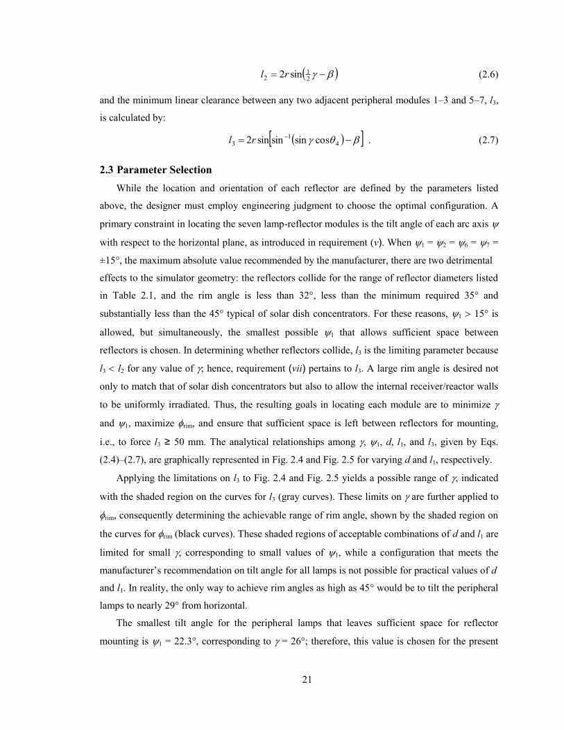
21

21

2 sin2rl (2.6)

and the minimum linear clearance between any two adjacent peripheral modules 1–3 and 5–7, l3,

is calculated by:

4

13 cossinsinsin2rl . (2.7)

2.3 Parameter Selection

While the location and orientation of each reflector are defined by the parameters listed

above, the designer must employ engineering judgment to choose the optimal configuration. A

primary constraint in locating the seven lamp-reflector modules is the tilt angle of each arc axis

with respect to the horizontal plane, as introduced in requirement (v). When 1 = 2 = 6 = 7 =

±15°, the maximum absolute value recommended by the manufacturer, there are two detrimental

effects to the simulator geometry: the reflectors collide for the range of reflector diameters listed

in Table 2.1, and the rim angle is less than 32°, less than the minimum required 35° and

substantially less than the 45° typical of solar dish concentrators. For these reasons, 1 15° is

allowed, but simultaneously, the smallest possible 1 that allows sufficient space between

reflectors is chosen. In determining whether reflectors collide, l3 is the limiting parameter because

l3 l2 for any value of ; hence, requirement (vii) pertains to l3. A large rim angle is desired not

only to match that of solar dish concentrators but also to allow the internal receiver/reactor walls

to be uniformly irradiated. Thus, the resulting goals in locating each module are to minimize

and 1, maximize rim, and ensure that sufficient space is left between reflectors for mounting,

i.e., to force l3 ≥ 50 mm. The analytical relationships among , 1, d, l1, and l3, given by Eqs.

(2.4)–(2.7), are graphically represented in Fig. 2.4 and Fig. 2.5 for varying d and l1, respectively.

Applying the limitations on l3 to Fig. 2.4 and Fig. 2.5 yields a possible range of , indicated

with the shaded region on the curves for l3 (gray curves). These limits on are further applied to

rim, consequently determining the achievable range of rim angle, shown by the shaded region on

the curves for rim (black curves). These shaded regions of acceptable combinations of d and l1 are

limited for small , corresponding to small values of 1, while a configuration that meets the

manufacturer’s recommendation on tilt angle for all lamps is not possible for practical values of d

and l1. In reality, the only way to achieve rim angles as high as 45° would be to tilt the peripheral

lamps to nearly 29° from horizontal.

The smallest tilt angle for the peripheral lamps that leaves sufficient space for reflector

mounting is 1 = 22.3°, corresponding to = 26°; therefore, this value is chosen for the present

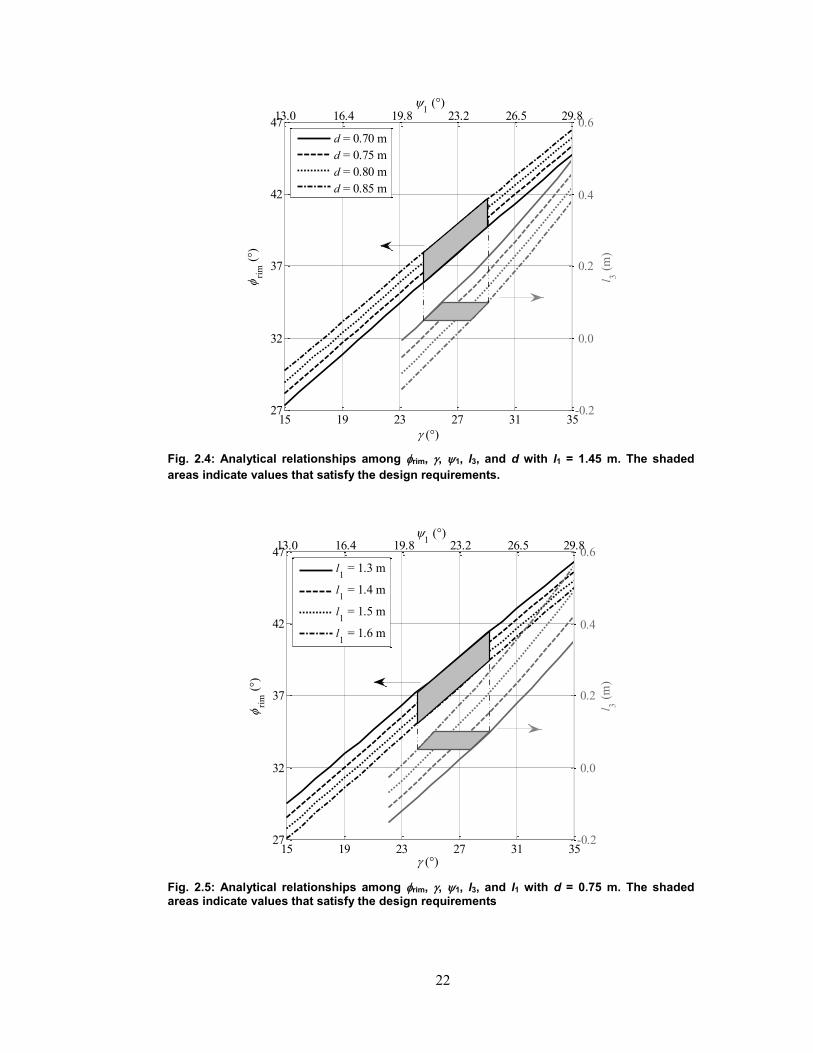
22

Fig. 2.4: Analytical relationships among rim, , 1, l3, and d with l1 = 1.45 m. The shaded

areas indicate values that satisfy the design requirements.

Fig. 2.5: Analytical relationships among rim, , 1, l3, and l1 with d = 0.75 m. The shaded areas indicate values that satisfy the design requirements

15 19 23 27 31 3527

32

37

42

47

(°)

ri

m (

°)

d = 0.70 m

d = 0.75 m

d = 0.80 m

d = 0.85 m

13.0 16.4 19.8 23.2 26.5 29.8

-0.2

0.0

0.2

0.4

0.6

l 3 (

m)

1 (°)

15 19 23 27 31 3527

32

37

42

47

(°)

ri

m (

°)

l1 = 1.3 m

l1 = 1.4 m

l1 = 1.5 m

l1 = 1.6 m

13.0 16.4 19.8 23.2 26.5 29.8

-0.2

0.0

0.2

0.4

0.6

l 3 (

m)

1 (°)

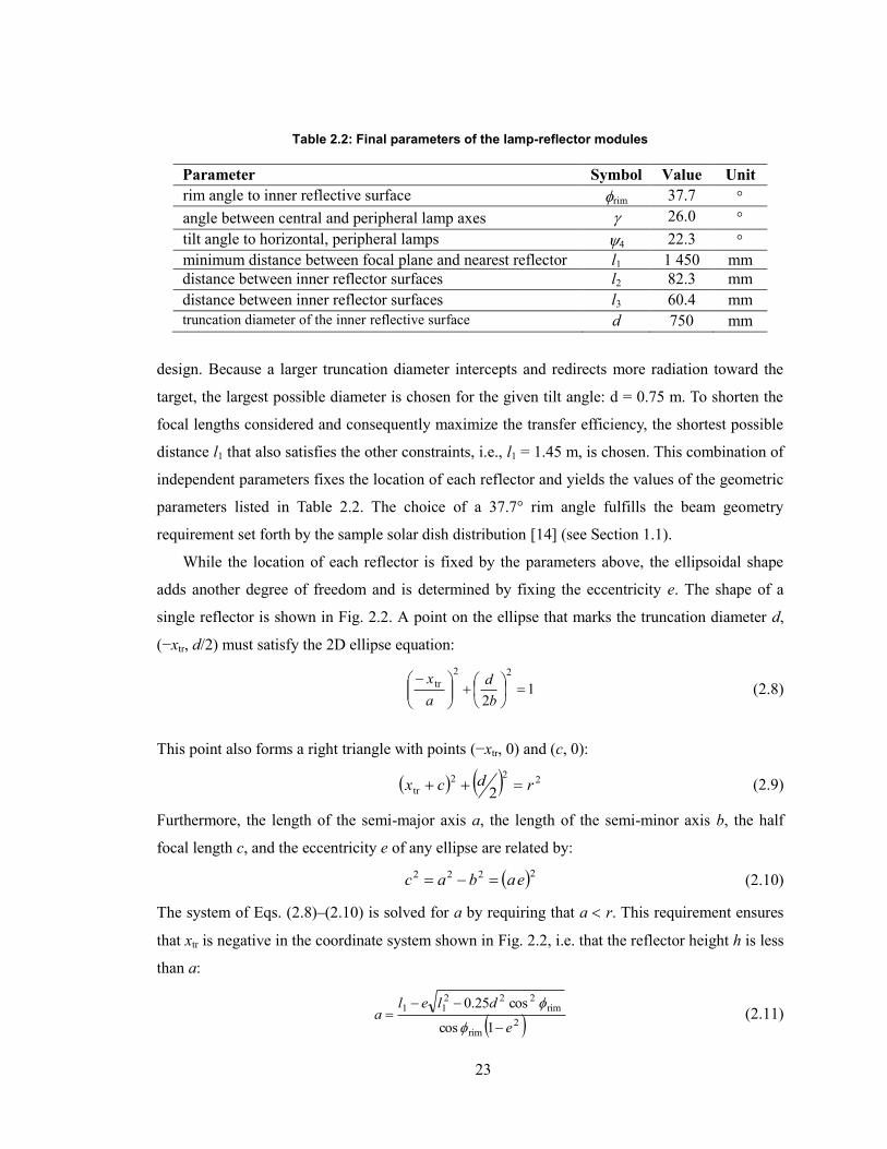
23

Table 2.2: Final parameters of the lamp-reflector modules

Parameter Symbol Value Unit

rim angle to inner reflective surface rim 37.7

angle between central and peripheral lamp axes 26.0

tilt angle to horizontal, peripheral lamps 4 22.3

minimum distance between focal plane and nearest reflector l1 1 450 mm

distance between inner reflector surfaces l2 82.3 mm

distance between inner reflector surfaces l3 60.4 mm

truncation diameter of the inner reflective surface d 750 mm

design. Because a larger truncation diameter intercepts and redirects more radiation toward the

target, the largest possible diameter is chosen for the given tilt angle: d = 0.75 m. To shorten the

focal lengths considered and consequently maximize the transfer efficiency, the shortest possible

distance l1 that also satisfies the other constraints, i.e., l1 = 1.45 m, is chosen. This combination of

independent parameters fixes the location of each reflector and yields the values of the geometric

parameters listed in Table 2.2. The choice of a 37.7° rim angle fulfills the beam geometry

requirement set forth by the sample solar dish distribution [14] (see Section 1.1).

While the location of each reflector is fixed by the parameters above, the ellipsoidal shape

adds another degree of freedom and is determined by fixing the eccentricity e. The shape of a

single reflector is shown in Fig. 2.2. A point on the ellipse that marks the truncation diameter d,

(−xtr, d/2) must satisfy the 2D ellipse equation:

12

22

tr

b

d

a

x (2.8)

This point also forms a right triangle with points (−xtr, 0) and (c, 0):

222

tr 2rdcx (2.9)

Furthermore, the length of the semi-major axis a, the length of the semi-minor axis b, the half

focal length c, and the eccentricity e of any ellipse are related by:

2222 eabac (2.10)

The system of Eqs. (2.8)–(2.10) is solved for a by requiring that a r. This requirement ensures

that xtr is negative in the coordinate system shown in Fig. 2.2, i.e. that the reflector height h is less

than a:

2

rim

rim222

11

1cos

cos25.0

e

dlela

(2.11)

24

The height of the reflector h is then calculated by

trxah , where eadrx 22tr 25.0 (2.12)

and has the requirement a–c ≤ h ≤ d, i.e., the center of the arc should be surrounded by the

reflector, but the reflector should be shorter than its diameter, a constraint that addresses

manufacturability concerns. The final parameters chosen based on these constraints and relations

are shown in Table 2.2 (see Fig. 2.1 and Fig. 2.2). The ellipsoid eccentricity determines the shape

of the reflector and contributes a further degree of freedom in the solar simulator design. The

method for optimizing the reflector shape is addressed in Chapter 3.

2.4 Summary

The solar simulator design combines seven 6.5 kWe xenon arc lamps, each coupled to a

reflector in the shape of an ellipsoid of revolution, in order to provide concentrated flux and

radiative power to the focal region. Xenon arc lamps are chosen as the artificial source of

radiation because the emission spectrum matches the solar spectral distribution (quantified by

AM 1.5 [22]) reasonably well, and the arc size is significantly smaller than than other artificial

radiation sources with spectral distributions. Additionally, the design procedure is outlined for

determining the location and orientation of any odd number of circularly-arranged lamp-reflector

modules with one module centrally located to ensure that their focal points coincide. A series of

unique geometric relations is developed to relate the dependent design parameters—the rim

angle, angle of peripheral lamp axes to the horizontal plane, and clearance between inner

reflective surfaces—to the independent design parameters, consisting of the angle between central

and peripheral lamp axes, minimum distance between focal plane and nearest point of a reflector,

and the reflector diameter. Using these geometric relations, the final design is determined to

consist of seven 6.5 kWe xenon short-arc lamps, each coupled to an ellipsoidal reflector with

truncation diameter of 750 mm. The array of lamp-reflector modules is arranged to result with a

minimum distance between the focal plane and the nearest point of a reflector of 1,450 mm, an

angle between central and peripheral lamp axes of 26.0°, a maximum tilt angle of any lamp axis

with respect to the horizontal plane of 22.3°, a rim angle of 37.7°, and a minimum clearance

between inner reflector surfaces of 60.4 mm. The final degree of freedom in the solar simulator

design is the shape of the reflector, quantified by its eccentricity. The eccentricity is optimized

according to the procedure set forth in Chapter 3.

25

Chapter 3

Reflector Optimization and Predicted Simulator Performance

The Monte Carlo ray tracing method is used to predict the radiative transport of the lamp-

reflector modules that comprise the University of Minnesota solar simulator and to optimize the

reflector shape. Individual radiation units, each comprised of a cylindrical source and a reflector,

are modeled separately. The radiative transport to the common focal plane is separately calculated

for each unit so that the outputs may be independently analyzed and superposed in any

combination. This approach allows the examination of flux distributions generated by varying

numbers of radiation units operating concurrently. Additionally, sensitivity analyses are

completed to determine the effect of the size and geometry of the arc, as well as the reflector

surface quality. The open-source code VeGas is used as the tool for these computations [46].

The optimization is carried out by altering the shape of the reflector, quantified by the

eccentricity e. The computed fluxes are used to calculate the transfer efficiency and the flux non-

uniformity, which are used as figures of merit in the optimization and measures of performance

for the completed simulator. The transfer efficiency is defined as the fraction of radiation

leaving the arc that arrives at the target, and the flux non-uniformity f is defined as the standard

deviation of flux incident in the focal plane and provides a metric for the flux distribution. An

optimized reflector geometry maximizes (consequently maximizing the amount of radiative

power at the target) and should yield an acceptable value of f. Section 3.3 contains further

details on these quantities and desired optimization outcomes.

3.1 Monte Carlo Ray Tracing Method

The Monte Carlo method employs stochastic sampling to model independent variables that

can be approximated using statistical models of a variety of physical systems, and ray tracing

tracks the paths of the rays to determine the thermal radiative transport with system components.

The ray approximation is used to calculate radiative transport, meaning that the radiative energy

emitted from a source is divided into a finite number of discrete energy bundles (rays) and that

the wavelength is significantly smaller than the media with which the ray interacts. The initial

location, direction, and wavelength of a ray are determined by the stochastic Monte Carlo method

[47–50]. The path of the ray is observed and its history is tracked as it interacts with surfaces and

participating media modeled in the system, which can act as transmitters, reflectors, scatterers, or

absorbers. A ray is determined to intersect a surface based on its origin point and direction, and

on the geometry and location of the surface. When a ray intersects a surface, its future behavior is

26

determined by the physics of the material (reflectivity and surface characteristics). In systems

with non-participating media, the ray may either be absorbed or reflected. If the ray is reflected,

its reflected direction is calculated and its path is further traced until it is absorbed or leaves the

system. The number of rays absorbed by each surface is tabulated throughout the Monte Carlo

simulation and is used to calculate the total energy absorbed by the surface. This process is

repeated for each ray. The general statistical Monte Carlo relations, presented here for

background, and those specific for thermal radiative transport, are paraphrased from Modest [48]

and Kalos and Whitlock [49].

3.1.1 Assumptions

In this study, only the energy associated with a light wave is accounted for, while information

about the phase of the wave is not tracked. This assumption does not affect the present work

because the goal result of the study is the distribution of energy, and not the phase of the waves

that are incident at the focal plane. Furthermore, the wavelength of the electromagnetic waves is

assumed to be significantly smaller than the geometry of the optics modeled here, in order to

avoid concerns of phase interference during reflection. The rays’ interactions follow the Markov

chain, in which each new interaction is assumed to be completely independent of all prior events

[50]. The stochastic nature of the analysis also requires that a large number of rays are used in

order to minimize systematic errors introduced by insufficiently sampling the system parameters.

The current analysis of the solar simulator assumes that reflection is independent of radiation

wavelength (gray). Although the emitted radiation may have spectral dependence, the desired

resulting quantity is the total amount of energy delivered, rather than its spectral distribution, so

the gray assumption may be used. For the comparative analyses of this study, attenuation of

radiation by the plasma arcs, the xenon gas inside the lamps, and the quartz envelopes of the

lamps is expected to influence all simulations equally and is therefore neglected. The

surroundings are assumed to be non-participating (cold and black) and reradiation from all

surfaces is neglected. The target is not allowed to reradiate because only the distribution of flux

incident on the target is important, while the high reflectivity of the ellipsoid reflectors leads to a

low absorbed heat flux and a negligible increase in surface temperature.

3.1.2 Fundamental Monte Carlo principles

The physical behavior of any system modeled with the Monte Carlo method, including the

parameters to be used in ray tracing, is captured with the statistical frequency function f. The

frequency function describes the distribution of the values that a certain property physically

27

possesses, or the frequency with which a variable takes on a particular value. The probability

density function g is a normalized representation of the frequency function:

nn

nn

xxxxxxf

xxxfxxxg

ddd,,

,,,,

2121

2121

(3.1)

The cumulative density function, G:

1 2 3

**2

*1

**2

*121 ddd,,,,

x x x

nnn xxxxxxgxxxG (3.2)

of a continuous function represents the likelihood that a random variable X occurs within the

interval set by the limits of integration. For a set of independent parameters, the cumulative

density function may be represented by the product of independent cumulative density functions:

nnn xGxGxGxxxG 221121 ,, (3.3)

Furthermore, an independent cumulative density function G(xi) of an independent parameter xi

may be calculated by:

ix

iii xxxxxxgxG **2

*1

**2

*1 ddd,,

(3.4)

The cumulative density function posses the property that G(∞) = 1. Because 0 ≤ G(xi) ≤ 1, G can

be equated to a random number i for the ith independent parameter xi of the physical system.

Inverting G(xi) allows the user to obtain a random value of the physical parameter:

ii xG 1 (3.5)

For thermal radiation, the physical parameters are emission locations, directions, and wavelength

(, r, z, , , , etc.) of an emitted ray, as required by the system to be modeled. The relations that

are specifically used to model the UMN solar simulator (including those for ray emission and

reflection) and their relations to random variables are outlined in Section 0.

3.1.3 Ray emission relations

Complete definition of a ray requires a specified wavelength, power, point of origin P0, and

directional unit vector .u The general geometric description is:

0ˆ01 uPP (3.6)

where P1 is another point along the ray. Once the ray tracing portion of the program begins, this

point is often taken as the intersection point with a surface in the system (to be determined). The

equation of the line following the ray’s path from P0 to P1 is given by:

uDPP ˆ01 (3.7)

28

where D is a length parameter for the distance separating P1 and P0.

The point of emission P0 for a new ray is determined with the use of probability density

functions that are specific to the source geometry and the type of emitter considered. If the source

is uniformly emitting, either from the volume or the surface, each location contained by the

geometry volume or surface, respectively, has equal probability of selection. Example relations

for a cylindrical source that emits uniformly from its volume, which is the source type used to

model the solar simulator, are provided in Section 3.3.

The direction and wavelength parameters for a ray’s emission are related by the probability

density function ge for either surface emission or volumetric emission in an isotropic medium.

The independent parameters for surface emission are two directional angles and , the azimuth

and polar angles, respectively, as well as temperature T and wavelength . Isotropic volumetric

emission requires definition of T and only. The probability density function describes the

relative likelihood that a random value of , , or will assume a particular value. It is used to

calculate the cumulative distribution functions of emission for each independent parameter (Ge,,

Ge,, Ge,), which are used to relate a random number (e,, e,, e,) ranging from 0 to 1 to the

corresponding wavelength or direction parameter for emission.

Probability density functions for surface and isotropic volumetric emission are outlined in

Modest [48]. The cumulative density functions used to determine polar angle and azimuth angle

of a ray emitted from an isotropic volume are depicted in Table 3.1, and their derivations are

also outlined by Modest. Isotropic (propagating with equal probability in all directions)

volumetric emission relations are highlighted here because the cylindrical source that is used to

model the xenon arc in the solar simulator lamps is assumed to emit uniformly from its isotropic

volume. In these relations, p is the Planck mean absorption coefficient, which is defined from the

spectral absorption coefficient for isotropic participating media and the spectral blackbody

intensity Ib as:

4

0

b

0

b

0

b

p

d,,

d,

d,,

T

TIT

TI

TIT

(3.8)

Table 3.1: Cumulative density functions for , , and for isotropic volumetric emission

Variable Type Cumulative Density Function

29

Polar angle Isotropic

Gray

2

cos1d

4

sin2*

0

4p

*4p

,e,e

*

θ

θT

TG (3.9)

Azimuth angle Isotropic

Gray

.2

d 2

1

d d4

sin

*

0

*

0 0

4p

4p

,e,e

*

*

ψ

ψT

TψG

ψ

ψ

ψ

ψ

ψψ

(3.10)

The direction unit vector of the ray u is calculated from the random geometric parameters

and by:

,ˆcosˆsinˆcossinˆ21 nttu (3.11)

where the tangential components 1t and 2t form a local right-handed coordinate system with the

normal component n .

3.1.4 Ray and surface interactions

Once the ray has been launched, the ray tracing portion of the model is used. A ray is

determined to intersect a surface by considering its general geometric equations, Eqs. (3.6) and

(3.7), and the geometric descriptions of the surfaces. Point P1 in the ray equations is constrained

by the geometric description of each surface in the system. Simultaneous solving of Eq. (3.7) and

the equation describing the surface determines an analytical expression for a length parameter D,

which is then used again in Eq. (3.7) to calculate P1. If P1 lies within the surface boundaries (for

example, if the distance between P1 and the center of a circular surface is less than the circle’s

radius), the ray intersects the surface. The intersection conditions are examined for each surface

in the system until an intersection point is reached. If these conditions are met for more than one

surface, the surface with the smallest length parameter is chosen because that surface is closest to

the ray origin point. If the conditions cannot be met for any surface, the ray is terminated (exits

the system) and does not interact with any component.

When a ray intersects an opaque surface with a total hemispherical reflectivity , a random

number is generated to determine whether the ray is reflected or absorbed. The ray is reflected

if Eq. (3.12) is satisfied:

. (3.12)

If Eq. (3.12) is not satisfied, the ray is absorbed and the internal counter for the surface is

increased by one. The ray’s reflected direction depends on the reflective character of the surface.

30

Specular reflectors, diffuse reflectors, and partially specular reflectors with error each require

different methods of determining the direction of a reflected ray, and all require calculation of the

surface normal vector. The surface normal is calculated by first describing the surface as a

geometric function of the global coordinate system. In the Cartesian coordinate system, a general

surface s is described by:

0,, zyxss (3.13)

The unit normal vector is then calculated by:

,

ˆˆˆ

ˆ222

z

s

y

s

x

s

kz

sj

y

si

x

s

s

sn (3.14)

and the two tangential vectors of the local coordinate system 1t and 2t are calculated by:

.ˆˆˆ,0ˆˆ121 tntnt (3.15)

The unit vector ru in the direction of a ray that has been reflected from a specular surface is

determined by considering the unit vector of the incident direction u and the unit normal vector

of the surface n by:

.ˆ)ˆˆ(2ˆˆr nnuuu (3.16)

Reflections from real surfaces perfectly specularly reflected, and the reflected rays are modified

by incorporating a specular error, s. A variety of methods can be used to account for s in the

direction of a reflected ray. They involve modifying the normal vector or modifying the reflected

ray, and both methods can be realized by modifying the vectors either by randomly generating a

polar and azimuth angle or by randomly generating two polar angles: one to be applied to each

tangential direction of the local coordinate system. The method of modifying the normal by

adjusting it with individual polar and azimuth angles is conceptually more realistic and is

therefore presented here. It should be noted that the code VeGas modifies the two tangential

components of the local coordinate system whose normal is coincident with the direction of the

ideally-reflected ray, and the specular error input to the code must be altered to match the

definition that modifies the polar and azimuth angles. Both methods require inputs of u , n , and

s:

s*r

*r ,ˆ,ˆˆˆ nuuu (3.17)

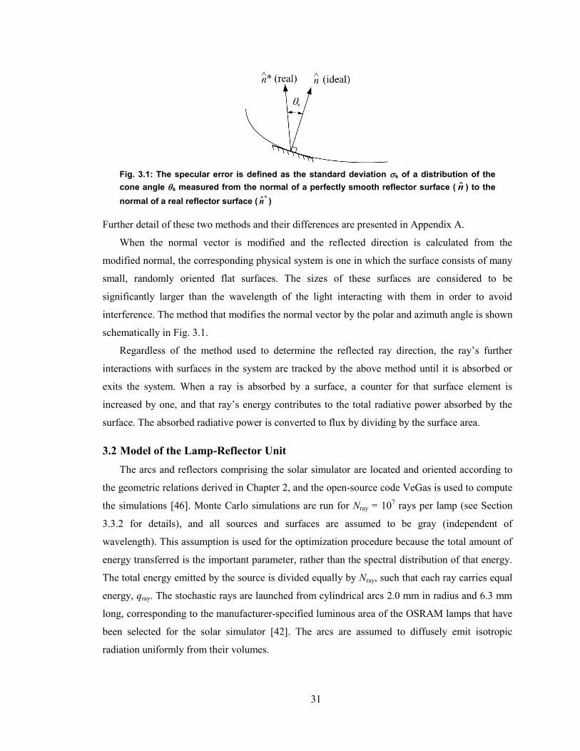
31

Fig. 3.1: The specular error is defined as the standard deviation s of a distribution of the

cone angle s measured from the normal of a perfectly smooth reflector surface ( n ) to the

normal of a real reflector surface (*

n )

Further detail of these two methods and their differences are presented in Appendix A.

When the normal vector is modified and the reflected direction is calculated from the

modified normal, the corresponding physical system is one in which the surface consists of many

small, randomly oriented flat surfaces. The sizes of these surfaces are considered to be

significantly larger than the wavelength of the light interacting with them in order to avoid

interference. The method that modifies the normal vector by the polar and azimuth angle is shown

schematically in Fig. 3.1.

Regardless of the method used to determine the reflected ray direction, the ray’s further

interactions with surfaces in the system are tracked by the above method until it is absorbed or

exits the system. When a ray is absorbed by a surface, a counter for that surface element is

increased by one, and that ray’s energy contributes to the total radiative power absorbed by the

surface. The absorbed radiative power is converted to flux by dividing by the surface area.

3.2 Model of the Lamp-Reflector Unit

The arcs and reflectors comprising the solar simulator are located and oriented according to

the geometric relations derived in Chapter 2, and the open-source code VeGas is used to compute

the simulations [46]. Monte Carlo simulations are run for Nray = 107 rays per lamp (see Section

3.3.2 for details), and all sources and surfaces are assumed to be gray (independent of

wavelength). This assumption is used for the optimization procedure because the total amount of

energy transferred is the important parameter, rather than the spectral distribution of that energy.

The total energy emitted by the source is divided equally by Nray, such that each ray carries equal

energy, qray. The stochastic rays are launched from cylindrical arcs 2.0 mm in radius and 6.3 mm

long, corresponding to the manufacturer-specified luminous area of the OSRAM lamps that have

been selected for the solar simulator [42]. The arcs are assumed to diffusely emit isotropic

radiation uniformly from their volumes.

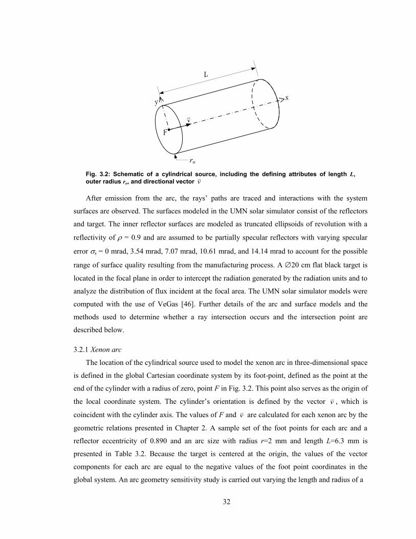
32

Fig. 3.2: Schematic of a cylindrical source, including the defining attributes of length L,

outer radius ro, and directional vector v

After emission from the arc, the rays’ paths are traced and interactions with the system

surfaces are observed. The surfaces modeled in the UMN solar simulator consist of the reflectors

and target. The inner reflector surfaces are modeled as truncated ellipsoids of revolution with a

reflectivity of = 0.9 and are assumed to be partially specular reflectors with varying specular

error s = 0 mrad, 3.54 mrad, 7.07 mrad, 10.61 mrad, and 14.14 mrad to account for the possible

range of surface quality resulting from the manufacturing process. A 20 cm flat black target is

located in the focal plane in order to intercept the radiation generated by the radiation units and to

analyze the distribution of flux incident at the focal area. The UMN solar simulator models were

computed with the use of VeGas [46]. Further details of the arc and surface models and the

methods used to determine whether a ray intersection occurs and the intersection point are

described below.

3.2.1 Xenon arc

The location of the cylindrical source used to model the xenon arc in three-dimensional space

is defined in the global Cartesian coordinate system by its foot-point, defined as the point at the

end of the cylinder with a radius of zero, point F in Fig. 3.2. This point also serves as the origin of

the local coordinate system. The cylinder’s orientation is defined by the vector v

, which is

coincident with the cylinder axis. The values of F and v

are calculated for each xenon arc by the

geometric relations presented in Chapter 2. A sample set of the foot points for each arc and a

reflector eccentricity of 0.890 and an arc size with radius r=2 mm and length L=6.3 mm is

presented in Table 3.2. Because the target is centered at the origin, the values of the vector

components for each arc are equal to the negative values of the foot point coordinates in the

global system. An arc geometry sensitivity study is carried out varying the length and radius of a

yx

v

F

L

ro

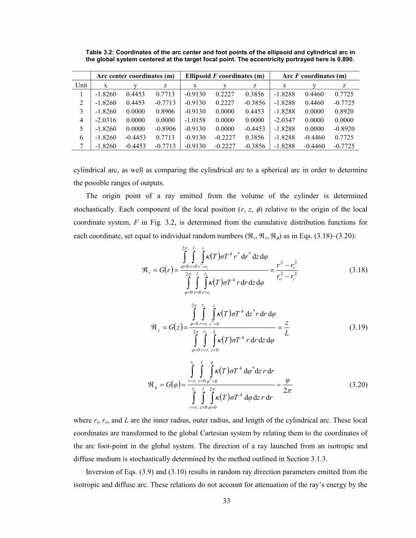
33

Table 3.2: Coordinates of the arc center and foot points of the ellipsoid and cylindrical arc in the global system centered at the target focal point. The eccentricity portrayed here is 0.890.

Arc center coordinates (m) Ellipsoid F coordinates (m) Arc F coordinates (m)

Unit x y z x y z x y z

1 -1.8260 0.4453 0.7713 -0.9130 0.2227 0.3856 -1.8288 0.4460 0.7725

2 -1.8260 0.4453 -0.7713 -0.9130 0.2227 -0.3856 -1.8288 0.4460 -0.7725

3 -1.8260 0.0000 0.8906 -0.9130 0.0000 0.4453 -1.8288 0.0000 0.8920

4 -2.0316 0.0000 0.0000 -1.0158 0.0000 0.0000 -2.0347 0.0000 0.0000

5 -1.8260 0.0000 -0.8906 -0.9130 0.0000 -0.4453 -1.8288 0.0000 -0.8920

6 -1.8260 -0.4453 0.7713 -0.9130 -0.2227 0.3856 -1.8288 -0.4460 0.7725

7 -1.8260 -0.4453 -0.7713 -0.9130 -0.2227 -0.3856 -1.8288 -0.4460 -0.7725

cylindrical arc, as well as comparing the cylindrical arc to a spherical arc in order to determine

the possible ranges of outputs.

The origin point of a ray emitted from the volume of the cylinder is determined

stochastically. Each component of the local position (r, z, ) relative to the origin of the local

coordinate system, F in Fig. 3.2, is determined from the cumulative distribution functions for

each coordinate, set equal to individual random numbers (r, z, ) as in Eqs. (3.18)–(3.20):

22

22

2

0 0

4

2

0 0

**4

ddd

ddd*

io

i

φ

l

z

r

rr

φ

l

z

r

rr

rrr

rr

φzrrσTT

φzrrσTT

rGo

i

i

(3.18)

L

z

φzrrσTT

φrrzσTT

zG

φ

r

rr

L

z

φ

r

rr

z

z

zo

i

o

i

2

0 0

4

2

0 0

*4

ddd

ddd*

(3.19)

2ddd

ddd

0

2

0

4

0 0

*4

* φ

rrzφσTT

rrzφσTT

φGo

i

o

i

r

rr

l

z φ

r

rr

l

z

φ

φ

φ

(3.20)

where ri, ro, and L are the inner radius, outer radius, and length of the cylindrical arc. These local

coordinates are transformed to the global Cartesian system by relating them to the coordinates of

the arc foot-point in the global system. The direction of a ray launched from an isotropic and

diffuse medium is stochastically determined by the method outlined in Section 3.1.3.

Inversion of Eqs. (3.9) and (3.10) results in random ray direction parameters emitted from the

isotropic and diffuse arc. These relations do not account for attenuation of the ray’s energy by the

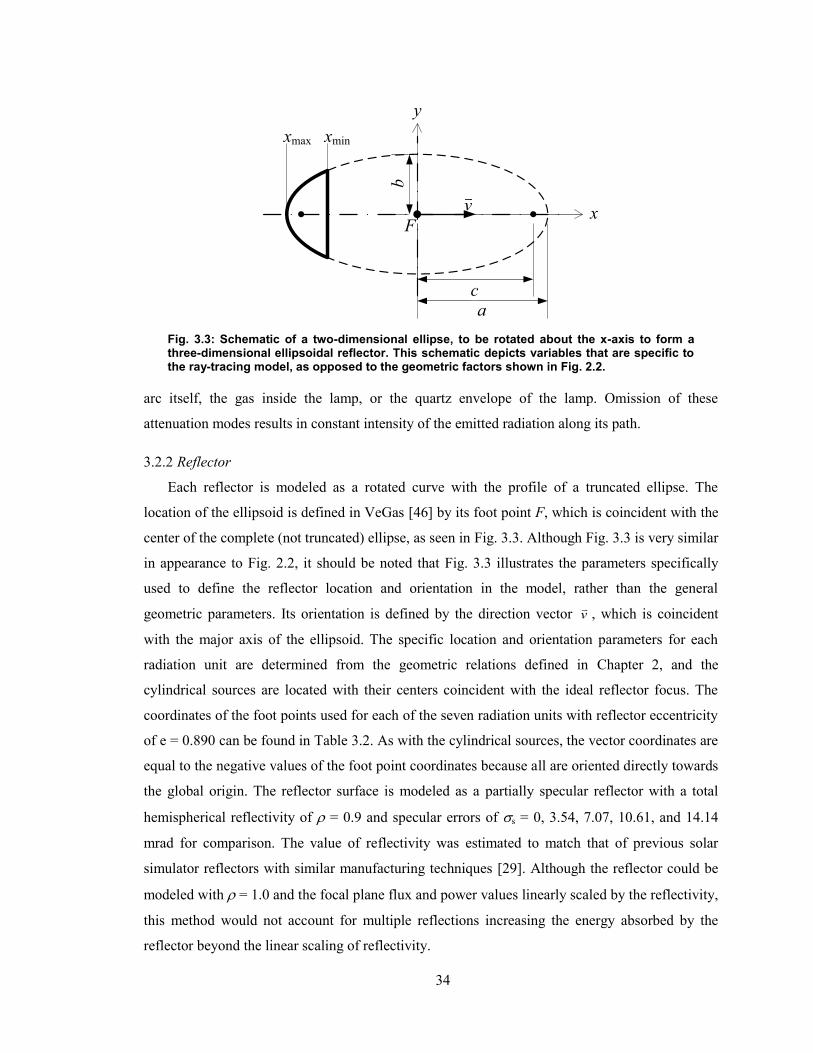
34

Fig. 3.3: Schematic of a two-dimensional ellipse, to be rotated about the x-axis to form a three-dimensional ellipsoidal reflector. This schematic depicts variables that are specific to the ray-tracing model, as opposed to the geometric factors shown in Fig. 2.2.

arc itself, the gas inside the lamp, or the quartz envelope of the lamp. Omission of these

attenuation modes results in constant intensity of the emitted radiation along its path.

3.2.2 Reflector

Each reflector is modeled as a rotated curve with the profile of a truncated ellipse. The

location of the ellipsoid is defined in VeGas [46] by its foot point F, which is coincident with the

center of the complete (not truncated) ellipse, as seen in Fig. 3.3. Although Fig. 3.3 is very similar

in appearance to Fig. 2.2, it should be noted that Fig. 3.3 illustrates the parameters specifically

used to define the reflector location and orientation in the model, rather than the general

geometric parameters. Its orientation is defined by the direction vector v

, which is coincident

with the major axis of the ellipsoid. The specific location and orientation parameters for each

radiation unit are determined from the geometric relations defined in Chapter 2, and the

cylindrical sources are located with their centers coincident with the ideal reflector focus. The

coordinates of the foot points used for each of the seven radiation units with reflector eccentricity

of e = 0.890 can be found in Table 3.2. As with the cylindrical sources, the vector coordinates are

equal to the negative values of the foot point coordinates because all are oriented directly towards

the global origin. The reflector surface is modeled as a partially specular reflector with a total

hemispherical reflectivity of = 0.9 and specular errors of s = 0, 3.54, 7.07, 10.61, and 14.14

mrad for comparison. The value of reflectivity was estimated to match that of previous solar

simulator reflectors with similar manufacturing techniques [29]. Although the reflector could be

modeled with = 1.0 and the focal plane flux and power values linearly scaled by the reflectivity,

this method would not account for multiple reflections increasing the energy absorbed by the

reflector beyond the linear scaling of reflectivity.

F

y

x

xminxmax

v

a

b

c

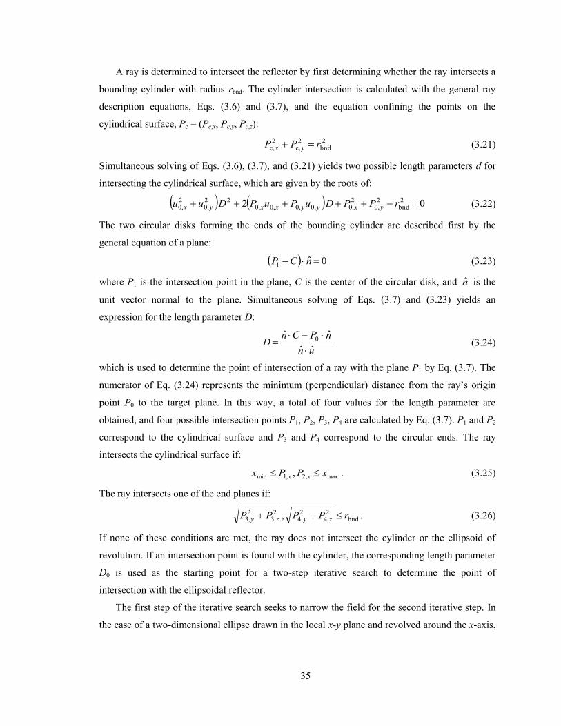
35

A ray is determined to intersect the reflector by first determining whether the ray intersects a

bounding cylinder with radius rbnd. The cylinder intersection is calculated with the general ray

description equations, Eqs. (3.6) and (3.7), and the equation confining the points on the

cylindrical surface, Pc = (Pc,x, Pc,y, Pc,z):

2

bnd2,c

2,c rPP yx (3.21)

Simultaneous solving of Eqs. (3.6), (3.7), and (3.21) yields two possible length parameters d for

intersecting the cylindrical surface, which are given by the roots of:

02 2bnd

2,0

2,0,0,0,0,0

22,0

2,0 rPPDuPuPDuu yxyyxxyx (3.22)

The two circular disks forming the ends of the bounding cylinder are described first by the

general equation of a plane:

0ˆ1 nCP (3.23)

where P1 is the intersection point in the plane, C is the center of the circular disk, and n is the

unit vector normal to the plane. Simultaneous solving of Eqs. (3.7) and (3.23) yields an

expression for the length parameter D:

un

nPCnD

ˆˆ

ˆˆ0

(3.24)

which is used to determine the point of intersection of a ray with the plane P1 by Eq. (3.7). The

numerator of Eq. (3.24) represents the minimum (perpendicular) distance from the ray’s origin

point P0 to the target plane. In this way, a total of four values for the length parameter are

obtained, and four possible intersection points P1, P2, P3, P4 are calculated by Eq. (3.7). P1 and P2

correspond to the cylindrical surface and P3 and P4 correspond to the circular ends. The ray

intersects the cylindrical surface if:

., max,2,1min xPPx xx (3.25)

The ray intersects one of the end planes if:

., bnd2,4

2,4

2,3

2,3 rPPPP zyzy (3.26)

If none of these conditions are met, the ray does not intersect the cylinder or the ellipsoid of

revolution. If an intersection point is found with the cylinder, the corresponding length parameter

D0 is used as the starting point for a two-step iterative search to determine the point of

intersection with the ellipsoidal reflector.

The first step of the iterative search seeks to narrow the field for the second iterative step. In

the case of a two-dimensional ellipse drawn in the local x-y plane and revolved around the x-axis,

36

as shown in Fig. 3.3 and used in the current study, the lengths of the two minor axes are equal. In

such a case, the general equation for the surface of an ellipsoid is:

.1

222

b

z

b

y

a

x (3.27)

A residual U, which is a measure of the distance between a general point P = (Px, Py, Pz), is

calculated from the general ellipsoid equation by:

222

2

2 bPPa

bPPU zyx

(3.28)

The residual is first calculated using point P0 as a reference. The length parameter that generated

the cylinder intersection point D0 is increased incrementally by D and is used to calculate a new

point 0P using Eq. (3.7):

uDDPP ˆ000 (3.29)

The residual is then calculated using the adjusted point 0P . If the signs of the two residuals

calculated with points P0 and 0P are not equal, then the point of intersection lies between the two

points and the iterative search for an intersection point proceeds to the second step. If the signs

are equal, the length parameter is increased by an additional D and the first iterative step is

repeated until the residual signs are unequal.

The second step of the iterative search for an intersection point with the rotated ellipsoid uses

the secant method of root finding, which employs the recurrence relation to generate increasingly

accurate approximations for the length parameter Dn:

uDPUuDPU

DDuDPUDD

nn

nnnnn

ˆˆˆ

2010

21101 (3.30)

A new value of the residual uDPU nˆ

0 is calculated by Eq. (3.28) from the updated length

parameter Dn and the process continues until the residual falls below a set maximum value. The

resulting length parameter is used to calculate the intersection point P1 by Eq. (3.7). If P1 satisfies

both Eq. (3.25) and Eq. (3.26), the ray intersects the reflector. If not, the ray misses the reflector

and its path is further followed until it is absorbed by another surface or leaves the system.

When a ray is incident on the reflector surface, the reflection condition (Eq. (3.12)) is

checked. If the ray is absorbed, the reflector segment intersected by the ray is determined by

matching the coordinates of point P1 to the coordinates of the finite elements, and the finite

element’s ray counter is increased by one to later verify that all rays are conserved. If the ray is

reflected, its new direction is calculated by the relations for a partially specular reflector (with

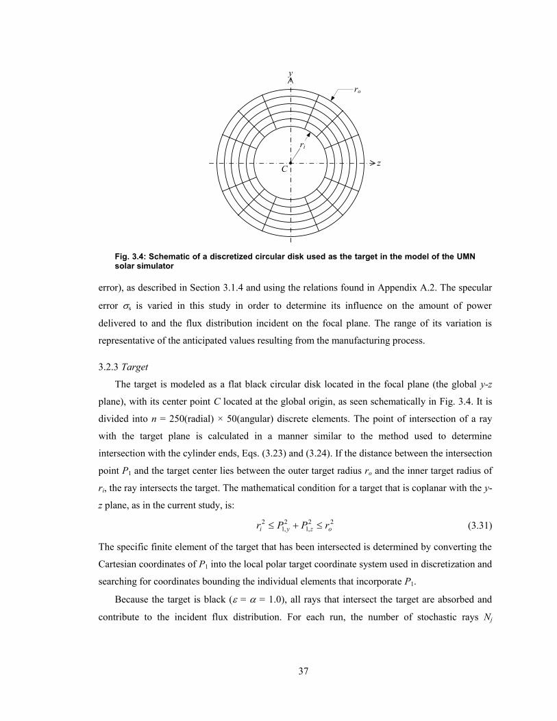
37

Fig. 3.4: Schematic of a discretized circular disk used as the target in the model of the UMN solar simulator

error), as described in Section 3.1.4 and using the relations found in Appendix A.2. The specular

error s is varied in this study in order to determine its influence on the amount of power

delivered to and the flux distribution incident on the focal plane. The range of its variation is

representative of the anticipated values resulting from the manufacturing process.

3.2.3 Target

The target is modeled as a flat black circular disk located in the focal plane (the global y-z

plane), with its center point C located at the global origin, as seen schematically in Fig. 3.4. It is

divided into n = 250(radial) × 50(angular) discrete elements. The point of intersection of a ray

with the target plane is calculated in a manner similar to the method used to determine

intersection with the cylinder ends, Eqs. (3.23) and (3.24). If the distance between the intersection

point P1 and the target center lies between the outer target radius ro and the inner target radius of

ri, the ray intersects the target. The mathematical condition for a target that is coplanar with the y-

z plane, as in the current study, is:

22

,12,1

2ozyi rPPr

(3.31)

The specific finite element of the target that has been intersected is determined by converting the

Cartesian coordinates of P1 into the local polar target coordinate system used in discretization and

searching for coordinates bounding the individual elements that incorporate P1.

Because the target is black ( = = 1.0), all rays that intersect the target are absorbed and

contribute to the incident flux distribution. For each run, the number of stochastic rays Nj

y

z

ro

ri

C

38

intercepted by each discrete element possessing area Aj of the target is computed. From these

data, the incident radiation at the finite target element is computed discretely by Eq. (3.32):

j

j

j

A

jA

qN

A

dAq

qj ray

(3.32)

A graphical summary of the Monte Carlo ray tracing method for thermal radiative transport

specific to this application can be seen in Fig. 3.5.

3.3 Single Reflector Optimization

Once the location and orientation of each of the seven lamp-reflector modules has been

determined, as outlined in Chapter 2, the simulator geometry is optimized by varying the shape of

the reflectors, as quantified by the eccentricity e (see Eq. (2.10)). The figures of merit used to

determine the optimal reflector shape are the transfer efficiency —defined as the fraction of

radiation leaving the sources that intercepts the target—and the flux non-uniformity f, described

here by the standard deviation2 of the flux distribution in the plane of interest (typically the focal

plane), weighted by the individual areas of target elements. The transfer efficiency provides a

method to estimate the amount of power and average flux that will be incident in the focal area,

while the flux uniformity quantifies the flux distribution. The figures of merit are defined

mathematically as follows:

M

i

ii

N

j

jj

Aq

Aq

1

1 (3.33)

N

j

j

jqq

A

A

q 1

2

tot

f

1

(3.34)

where M, N, iq , jq , and q are the number of radiation sources (arcs), the number of discrete

elements on the target, the radiative flux leaving the i-th source, the radiative flux intercepted by

the j-th discrete target element, and the average radiative flux incident on the target area

considered, respectively; Ai, Aj, and Atot are the surface areas of the i-th radiation source, the j-th

2 The standard deviation f is used to quantitatively estimate the degree of flux non-uniformity; however, this quantity should not

be interpreted as the standard deviation of a Gaussian distribution due to anticipated differences between the actual flux distribution and a Gaussian distribution.

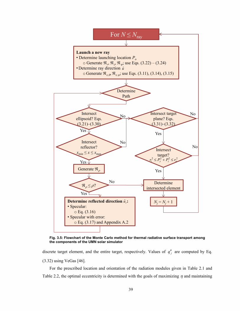
39

Fig. 3.5: Flowchart of the Monte Carlo method for thermal radiative surface transport among the components of the UMN solar simulator

discrete target element, and the entire target, respectively. Values of jq are computed by Eq.

(3.32) using VeGas [46].

For the prescribed location and orientation of the radiation modules given in Table 2.1 and

Table 2.2, the optimal eccentricity is determined with the goals of maximizing and maintaining

For N ≤ Nray

Launch a new ray

• Determine launching location Po

o Generate r, z, ; use Eqs. (3.22) – (3.24)

• Determine ray direction

oGenerate e,, e,; use Eqs. (3.11), (3.14), (3.15)

u

Determine

Path

Intersect

ellipsoid? Eqs.

(3.21)–(3.30)

Intersect target

plane? Eqs.

(3.31)–(3.32)

NoNo

Intersect

reflector?

xmin ≤ x ≤ xmax

Yes

No

Yes

Intersect

target?2222

ozyi rPPr

No

Nj = Nj + 1

Determine

intersected element

YesGenerate

Yes

≤ ?No

Determine reflected direction :

• Specular:

o Eq. (3.16)

• Specular with error:

o Eq. (3.17) and Appendix A.2

ru

Yes

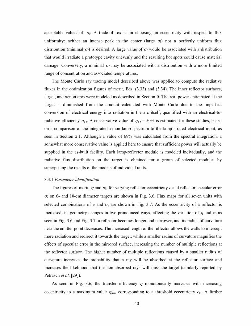
40

acceptable values of f. A trade-off exists in choosing an eccentricity with respect to flux

uniformity: neither an intense peak in the center (large f) nor a perfectly uniform flux

distribution (minimal f) is desired. A large value of f would be associated with a distribution

that would irradiate a prototype cavity unevenly and the resulting hot spots could cause material

damage. Conversely, a minimal f may be associated with a distribution with a more limited

range of concentration and associated temperatures.

The Monte Carlo ray tracing model described above was applied to compute the radiative

fluxes in the optimization figures of merit, Eqs. (3.33) and (3.34). The inner reflector surfaces,

target, and xenon arcs were modeled as described in Section 0. The real power anticipated at the

target is diminished from the amount calculated with Monte Carlo due to the imperfect

conversion of electrical energy into radiation in the arc itself, quantified with an electrical-to-

radiative efficiency e-r. A conservative value of e-r = 50% is estimated for these studies, based

on a comparison of the integrated xenon lamp spectrum to the lamp’s rated electrical input, as

seen in Section 2.1. Although a value of 69% was calculated from the spectral integration, a

somewhat more conservative value is applied here to ensure that sufficient power will actually be

supplied in the as-built facility. Each lamp-reflector module is modeled individually, and the

radiative flux distribution on the target is obtained for a group of selected modules by

superposing the results of the models of individual units.

3.3.1 Parameter identification

The figures of merit, and f, for varying reflector eccentricity e and reflector specular error

s on 6- and 10-cm diameter targets are shown in Fig. 3.6. Flux maps for all seven units with

selected combinations of e and s are shown in Fig. 3.7. As the eccentricity of a reflector is

increased, its geometry changes in two pronounced ways, affecting the variation of and f as

seen in Fig. 3.6 and Fig. 3.7: a reflector becomes longer and narrower, and its radius of curvature

near the emitter point decreases. The increased length of the reflector allows the walls to intercept

more radiation and redirect it towards the target, while a smaller radius of curvature magnifies the

effects of specular error in the mirrored surface, increasing the number of multiple reflections at

the reflector surface. The higher number of multiple reflections caused by a smaller radius of

curvature increases the probability that a ray will be absorbed at the reflector surface and

increases the likelihood that the non-absorbed rays will miss the target (similarly reported by

Petrasch et al. [29]).

As seen in Fig. 3.6, the transfer efficiency monotonically increases with increasing

eccentricity to a maximum value max corresponding to a threshold eccentricity eth. A further

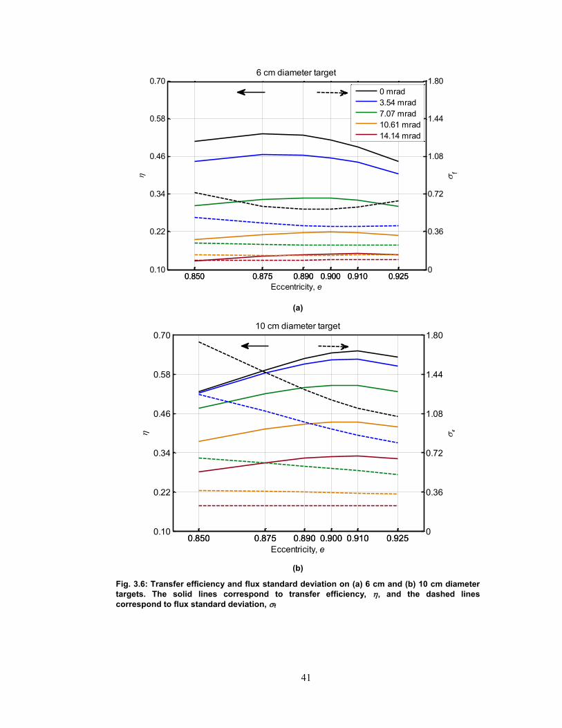
41

(a)

(b)

Fig. 3.6: Transfer efficiency and flux standard deviation on (a) 6 cm and (b) 10 cm diameter

targets. The solid lines correspond to transfer efficiency, , and the dashed lines

correspond to flux standard deviation, f

0.850 0.875 0.890 0.900 0.910 0.9250.10

0.22

0.34

0.46

0.58

0.70

0.850 0.875 0.890 0.900 0.910 0.9250

0.36

0.72

1.08

1.44

1.80

f

Eccentricity, e

6 cm diameter target

0 mrad

3.54 mrad

7.07 mrad

10.61 mrad

14.14 mrad

0.850 0.875 0.890 0.900 0.910 0.9250.10

0.22

0.34

0.46

0.58

0.70

0.850 0.875 0.890 0.900 0.910 0.9250

0.36

0.72

1.08

1.44

1.80

f

Eccentricity, e

10 cm diameter target

42

Fig. 3.7: Flux maps for the geometry listed in Table 2.1 and Table 2.2 with eccentricity e =

0.890 and varying values of specular error: (a) s = 0 mrad (b) s = 7.07 mrad (c) s = 14.14

mrad; and with specular error s = 7.07 mrad and varying values of eccentricity: (d) e = 0.850, (e) e = 0.900, (f) e = 0.925. The inner circle is 6 cm in diameter and the outer circle is 10 cm in diameter. Note that the scale differs for plot (a)–(c)

(a) (d)

(b)

(c)

(e)

(f)

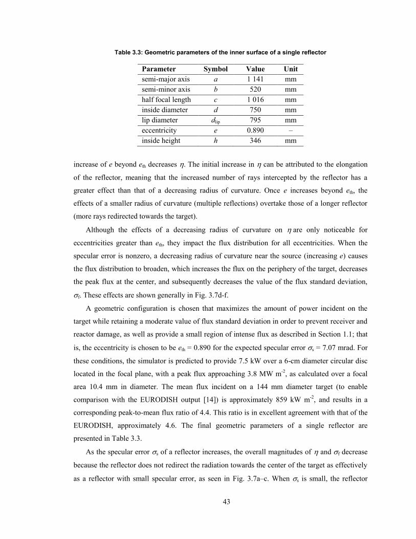
43

Table 3.3: Geometric parameters of the inner surface of a single reflector

Parameter Symbol Value Unit

semi-major axis a 1 141 mm

semi-minor axis b 520 mm

half focal length c 1 016 mm

inside diameter d 750 mm

lip diameter dlip 795 mm

eccentricity e 0.890 –

inside height h 346 mm

increase of e beyond eth decreases . The initial increase in can be attributed to the elongation

of the reflector, meaning that the increased number of rays intercepted by the reflector has a

greater effect than that of a decreasing radius of curvature. Once e increases beyond eth, the

effects of a smaller radius of curvature (multiple reflections) overtake those of a longer reflector

(more rays redirected towards the target).

Although the effects of a decreasing radius of curvature on are only noticeable for

eccentricities greater than eth, they impact the flux distribution for all eccentricities. When the

specular error is nonzero, a decreasing radius of curvature near the source (increasing e) causes

the flux distribution to broaden, which increases the flux on the periphery of the target, decreases

the peak flux at the center, and subsequently decreases the value of the flux standard deviation,

f. These effects are shown generally in Fig. 3.7d-f.

A geometric configuration is chosen that maximizes the amount of power incident on the

target while retaining a moderate value of flux standard deviation in order to prevent receiver and

reactor damage, as well as provide a small region of intense flux as described in Section 1.1; that

is, the eccentricity is chosen to be eth = 0.890 for the expected specular error s = 7.07 mrad. For

these conditions, the simulator is predicted to provide 7.5 kW over a 6-cm diameter circular disc

located in the focal plane, with a peak flux approaching 3.8 MW m-2

, as calculated over a focal

area 10.4 mm in diameter. The mean flux incident on a 144 mm diameter target (to enable

comparison with the EURODISH output [14]) is approximately 859 kW m-2

, and results in a

corresponding peak-to-mean flux ratio of 4.4. This ratio is in excellent agreement with that of the

EURODISH, approximately 4.6. The final geometric parameters of a single reflector are

presented in Table 3.3.

As the specular error s of a reflector increases, the overall magnitudes of and f decrease

because the reflector does not redirect the radiation towards the center of the target as effectively

as a reflector with small specular error, as seen in Fig. 3.7a–c. When s is small, the reflector

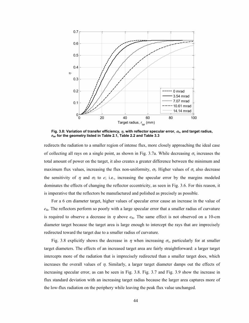
44

Fig. 3.8: Variation of transfer efficiency, , with reflector specular error, s, and target radius, rtar for the geometry listed in Table 2.1, Table 2.2 and Table 3.3

redirects the radiation to a smaller region of intense flux, more closely approaching the ideal case

of collecting all rays on a single point, as shown in Fig. 3.7a. While decreasing s increases the

total amount of power on the target, it also creates a greater difference between the minimum and

maximum flux values, increasing the flux non-uniformity, f. Higher values of s also decrease

the sensitivity of and f to e; i.e., increasing the specular error by the margins modeled

dominates the effects of changing the reflector eccentricity, as seen in Fig. 3.6. For this reason, it

is imperative that the reflectors be manufactured and polished as precisely as possible.

For a 6 cm diameter target, higher values of specular error cause an increase in the value of

eth. The reflectors perform so poorly with a large specular error that a smaller radius of curvature

is required to observe a decrease in above eth. The same effect is not observed on a 10-cm

diameter target because the target area is large enough to intercept the rays that are imprecisely

redirected toward the target due to a smaller radius of curvature.

Fig. 3.8 explicitly shows the decrease in when increasing s, particularly for at smaller

target diameters. The effects of an increased target area are fairly straightforward: a larger target

intercepts more of the radiation that is imprecisely redirected than a smaller target does, which

increases the overall values of . Similarly, a larger target diameter damps out the effects of

increasing specular error, as can be seen in Fig. 3.8. Fig. 3.7 and Fig. 3.9 show the increase in

flux standard deviation with an increasing target radius because the larger area captures more of

the low-flux radiation on the periphery while leaving the peak flux value unchanged.

0 20 40 60 80 1000

0.1

0.2

0.3

0.4

0.5

0.6

0.7

Target radius, rtar

(mm)

0 mrad

3.54 mrad

7.07 mrad

10.61 mrad

14.14 mrad

45

Fig. 3.9: Variation of transfer efficiency, (solid line), and flux standard deviation, f (dashed

line), with target radius for the final geometry (Table 3.3) and s = 7.07 mrad using 108 rays

per lamp

When the output of all seven lamps is simultaneously observed, the flux distribution on the

target displays radial symmetry, as illustrated in Fig. 3.7 and Fig. 3.10. Fig. 3.10 depicts

superposed cross-sectional profiles of the flux distribution along the y- and z-axes, and based on

the very similar profiles in each direction, it is clear that the distributions exhibit radial symmetry

in those two directions. Further observation of Fig. 3.7 indicates that there are no deviations from

this symmetry in other directions. The variations of the cumulative average flux and power with

increasing radius are shown in Fig. 3.11. The average flux reaches a maximum as rtar 0, and

decreases with increasing target radius due to the relatively small increase in incident power

compared to the larger increase in area. The intercepted power increases rapidly with increasing

target radius due to the large increase in the area of the target.

An additional parameter to be studied in a sensitivity analysis is the effective arc geometry

and size. The real plasma arc is not expected to behave like the cylinder emitting isotropically and

uniformly from its volume assumed in this study. The lamp manufacturers have indicated that the

arc resembles a small area of very intense emission generated by the plasma ball at the tip of the

cathode with larger areas of decreasing emission closer to the anode, as shown in Fig. 3.12

[42,51]. The pointed shape of the cathode causes a higher concentration of ions in its immediate

vicinity (as opposed to the broad, flat anode), causing an increase in the photons released and

higher emitted radiative intensity. Although an isotropic and uniformly emitting cylinder or

sphere cannot capture the complexity associated with such an arc, the size and shape of the

0 20 40 60 80 1000.00

0.07

0.14

0.21

0.28

0.35

0.42

0.49

0.56

0.63

0.70

0 20 40 60 80 1000.0

0.2

0.4

0.6

0.8

1.0

1.2

1.4

1.6

1.8

2.0

f

Target radius rtar

(mm)

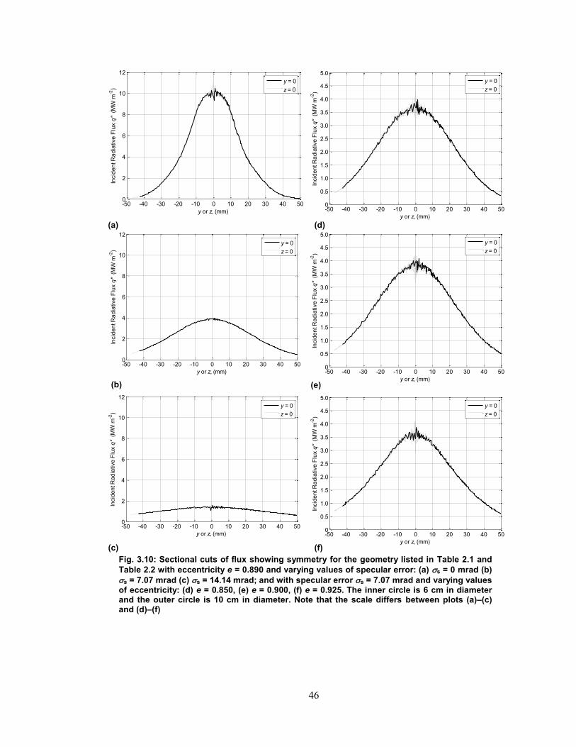
46

Fig. 3.10: Sectional cuts of flux showing symmetry for the geometry listed in Table 2.1 and

Table 2.2 with eccentricity e = 0.890 and varying values of specular error: (a) s = 0 mrad (b)

s = 7.07 mrad (c) s = 14.14 mrad; and with specular error s = 7.07 mrad and varying values of eccentricity: (d) e = 0.850, (e) e = 0.900, (f) e = 0.925. The inner circle is 6 cm in diameter and the outer circle is 10 cm in diameter. Note that the scale differs between plots (a)–(c) and (d)–(f)

-50 -40 -30 -20 -10 0 10 20 30 40 500

2

4

6

8

10

12

y or z, (mm)

Incid

en

t R

ad

iative

Flu

x q"

(M

W m

-2)

y = 0

z = 0

-50 -40 -30 -20 -10 0 10 20 30 40 500

0.5

1.0

1.5

2.0

2.5

3.0

3.5

4.0

4.5

5.0

y or z, (mm)

Incid

en

t R

ad

iative

Flu

x q"

(M

W m

-2)

y = 0

z = 0

-50 -40 -30 -20 -10 0 10 20 30 40 500

2

4

6

8

10

12

y or z, (mm)

Incid

en

t R

ad

iative

Flu

x q"

(M

W m

-2)

y = 0

z = 0

-50 -40 -30 -20 -10 0 10 20 30 40 500

0.5

1.0

1.5

2.0

2.5

3.0

3.5

4.0

4.5

5.0

y or z, (mm)

Incid

en

t R

ad

iative

Flu

x q"

(M

W m

-2)

y = 0

z = 0

-50 -40 -30 -20 -10 0 10 20 30 40 500

2

4

6

8

10

12

y or z, (mm)

Incid

en

t R

ad

iative

Flu

x q"

(M

W m

-2)

y = 0

z = 0

-50 -40 -30 -20 -10 0 10 20 30 40 500

0.5

1.0

1.5

2.0

2.5

3.0

3.5

4.0

4.5

5.0

y or z, (mm)

Incid

en

t R

ad

iative

Flu

x q"

(M

W m

-2)

y = 0

z = 0

(d) (a)

(e) (b)

(c) (f)

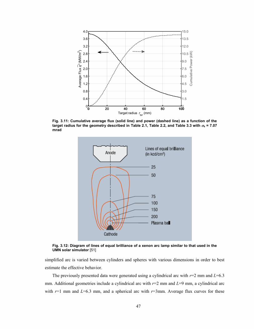
47

Fig. 3.11: Cumulative average flux (solid line) and power (dashed line) as a function of the

target radius for the geometry described in Table 2.1, Table 2.2, and Table 3.3 with s = 7.07 mrad

Fig. 3.12: Diagram of lines of equal brilliance of a xenon arc lamp similar to that used in the UMN solar simulator [51]

simplified arc is varied between cylinders and spheres with various dimensions in order to best

estimate the effective behavior.

The previously presented data were generated using a cylindrical arc with r=2 mm and L=6.3

mm. Additional geometries include a cylindrical arc with r=2 mm and L=9 mm, a cylindrical arc

with r=1 mm and L=6.3 mm, and a spherical arc with r=3mm. Average flux curves for these

0 20 40 60 80 1000

0.4

0.8

1.2

1.6

2.0

2.4

2.8

3.2

3.6

4.0

Ave

rag

e F

lux q

" (M

W/m

2)

0 20 40 60 80 1000

1.5

3.0

4.5

6.0

7.5

9.0

10.5

12.0

13.5

15.0

Cu

mu

lative

Po

we

r (k

W)

Target radius rtar

(mm)

|

48

Fig. 3.13: Cumulative average flux curves for varying arc size and geometry

geometries are shown in Fig. 3.13. It is generally shown that the average incident flux at a given

target radius decreases with an increasing volume of a cylindrical arc. The center of each arc

shape is located at the ideal focus of the ellipsoidal reflector, so the larger arcs allow rays to be

launched farther from the ideal focus. As previously discussed, the distance between the arrival

point and the ideal target focus increases with increasing distance between the launching point

and the ideal source focus. Although the spherical arc has the same volume as the largest

cylindrical arc, the maximum distance between a launching point and the ideal source focus is

greater for the cylinder than for the sphere. At a target radius of approximately 30 mm, the

cylinder with r=1 mm and L=6.3 mm predicts 25% more incident flux than the cylindrical arc

with r=2 mm and L=9 mm. The difference decreases to 15% at a target radius of approximately

40 mm. Because most of the work examined flux distributions 30 mm in radius or more (60 mm

diameter), the arc geometry contributes no more than 25% difference to the above results.

3.3.2 Accuracy Considerations

The stochastic nature of these numerical studies requires that many rays are used in order to

fully represent the distributions of the parameters. It is necessary to ensure that the results

generated are independent of both the number of rays launched from a source Nray, as well as the

discretization scheme of the target, regarding both the number of finite elements on the target and

their shapes. By comparing a standard model to one run with 108 rays per arc, it was determined

that simulations performed with 107 rays adequately eliminated the random influences of Monte

0 10 20 30 40 502

4

6

8

10

12

14

16

18

20

Target radius, rtar

(mm)

Ave

rag

e In

cid

en

t F

lux, q

" (

MW

m-2

)

Cylinderr =2mm, L=9mm

Spherer =3mm

Cylinderr =2mm, L=6.3mm

Cylinderr =1mm, L=6.3mm

49

Carlo simulations as long as the data examined were for target diameters of at least 30 mm. The

number of rays intercepting smaller target diameters is not great enough to give a statistically

meaningful result. Between simulations computed with 107 and 10

8 rays and s = 3.54 mrad,

solutions for vary no more than 0.02% while values of f vary no more than 0.2% when dtar ≥

28 mm. Similarly, when the target was discretized with a fine polar grid (500 radial 50 angular),

a standard polar grid (250 radial 50 angular), and a rectangular grid (188 188) with s = 3.54

mrad and 107 rays, values of cumulative flux vary less than 0.04% for a target diameter of

approximately 5.6 mm. In order for values of f to vary less than 1.0%, the target diameter must

be approximately 28 mm.

3.4 Summary

Monte Carlo ray tracing was used to model the radiative transport of the seven lamp-reflector

modules that comprise the solar simulator. Each xenon arc was modeled as a cylinder centered at

the focal point of its coupled ellipsoidal reflector, which was modeled with a reflectivity of 0.9

and varying values of specular error. The target was modeled as a flat black disk located in the

focal plane, and the surroundings were non-participating (cold and black). The independent

optimization parameter was the eccentricity of the ellipsoid, which defines the shape of the

reflector and was varied between 0.85 and 0.925. The goals of the optimization study were to

maximize the transfer of radiative energy from the arcs to the target while maintaining a

reasonable distribution of flux. It was determined that a trade-off exists in these two

requirements: a very clear maximum in transfer efficiency occurs with a particular eccentricity,

but if the eccentricity is varied only a small amount from the one that results in maximum power

transfer, the transfer efficiency significantly decreases. For this reason, the designer was forced to

select the eccentricity that resulted in the most power delivered to the target, regardless of the flux

distribution in the focal plane, which is 0.890 when the specular error is assumed to be 7.07 mrad.

The selection of the eccentricity, along with the parameters determined in Chapter 2, fully define

the design of the UMN solar simulator. Based on the model described above, the simulator is

predicted to provide 7.5 kW over a 6-cm diameter circular disc located in the focal plane, with a

peak flux approaching 3700 kW m-2

.

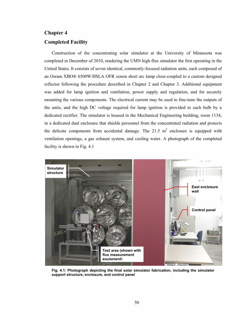
50

Chapter 4

Completed Facility

Construction of the concentrating solar simulator at the University of Minnesota was

completed in December of 2010, rendering the UMN high-flux simulator the first operating in the

United States. It consists of seven identical, commonly-focused radiation units, each composed of

an Osram XBO® 6500W/HSLA OFR xenon short arc lamp close-coupled to a custom designed

reflector following the procedure described in Chapter 2 and Chapter 3. Additional equipment

was added for lamp ignition and ventilation, power supply and regulation, and for securely

mounting the various components. The electrical current may be used to fine-tune the outputs of

the units, and the high DC voltage required for lamp ignition is provided to each bulb by a

dedicated rectifier. The simulator is housed in the Mechanical Engineering building, room 1134,

in a dedicated dual enclosure that shields personnel from the concentrated radiation and protects

the delicate components from accidental damage. The 21.5 m2 enclosure is equipped with

ventilation openings, a gas exhaust system, and cooling water. A photograph of the completed

facility is shown in Fig. 4.1

Fig. 4.1: Photograph depicting the final solar simulator fabrication, including the simulator support structure, enclosure, and control panel

Simulator

structure

Test area (shown with flux measurement equipment)

Control panel

East enclosure

wall

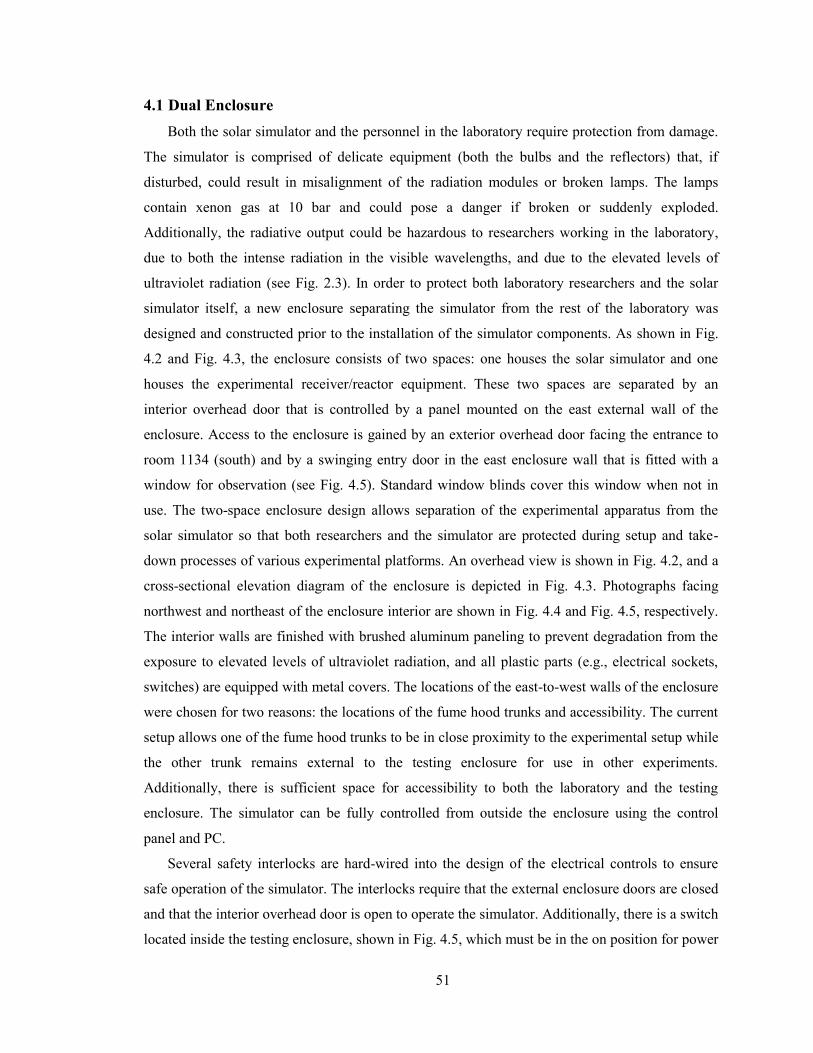
51

4.1 Dual Enclosure

Both the solar simulator and the personnel in the laboratory require protection from damage.

The simulator is comprised of delicate equipment (both the bulbs and the reflectors) that, if

disturbed, could result in misalignment of the radiation modules or broken lamps. The lamps

contain xenon gas at 10 bar and could pose a danger if broken or suddenly exploded.

Additionally, the radiative output could be hazardous to researchers working in the laboratory,

due to both the intense radiation in the visible wavelengths, and due to the elevated levels of

ultraviolet radiation (see Fig. 2.3). In order to protect both laboratory researchers and the solar

simulator itself, a new enclosure separating the simulator from the rest of the laboratory was

designed and constructed prior to the installation of the simulator components. As shown in Fig.

4.2 and Fig. 4.3, the enclosure consists of two spaces: one houses the solar simulator and one

houses the experimental receiver/reactor equipment. These two spaces are separated by an

interior overhead door that is controlled by a panel mounted on the east external wall of the

enclosure. Access to the enclosure is gained by an exterior overhead door facing the entrance to

room 1134 (south) and by a swinging entry door in the east enclosure wall that is fitted with a

window for observation (see Fig. 4.5). Standard window blinds cover this window when not in

use. The two-space enclosure design allows separation of the experimental apparatus from the

solar simulator so that both researchers and the simulator are protected during setup and take-

down processes of various experimental platforms. An overhead view is shown in Fig. 4.2, and a

cross-sectional elevation diagram of the enclosure is depicted in Fig. 4.3. Photographs facing

northwest and northeast of the enclosure interior are shown in Fig. 4.4 and Fig. 4.5, respectively.

The interior walls are finished with brushed aluminum paneling to prevent degradation from the

exposure to elevated levels of ultraviolet radiation, and all plastic parts (e.g., electrical sockets,

switches) are equipped with metal covers. The locations of the east-to-west walls of the enclosure

were chosen for two reasons: the locations of the fume hood trunks and accessibility. The current

setup allows one of the fume hood trunks to be in close proximity to the experimental setup while

the other trunk remains external to the testing enclosure for use in other experiments.

Additionally, there is sufficient space for accessibility to both the laboratory and the testing

enclosure. The simulator can be fully controlled from outside the enclosure using the control

panel and PC.

Several safety interlocks are hard-wired into the design of the electrical controls to ensure

safe operation of the simulator. The interlocks require that the external enclosure doors are closed

and that the interior overhead door is open to operate the simulator. Additionally, there is a switch

located inside the testing enclosure, shown in Fig. 4.5, which must be in the on position for power

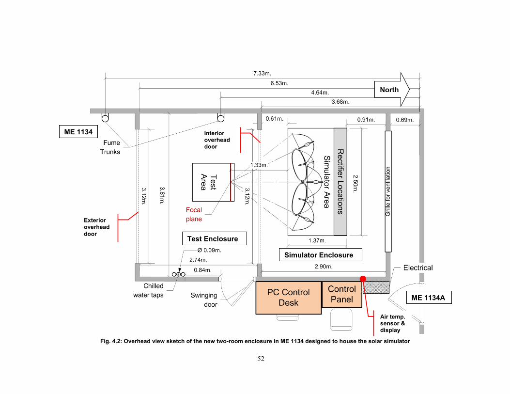
52

Fig. 4.2: Overhead view sketch of the new two-room enclosure in ME 1134 designed to house the solar simulator

North

Interior overhead door

Exterior overhead

door

ME 1134A

Test Enclosure

Simulator Enclosure

ME 1134

Air temp. sensor & display

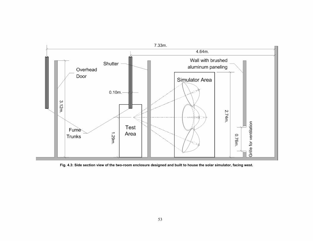
53

Fig. 4.3: Side section view of the two-room enclosure designed and built to house the solar simulator, facing west.

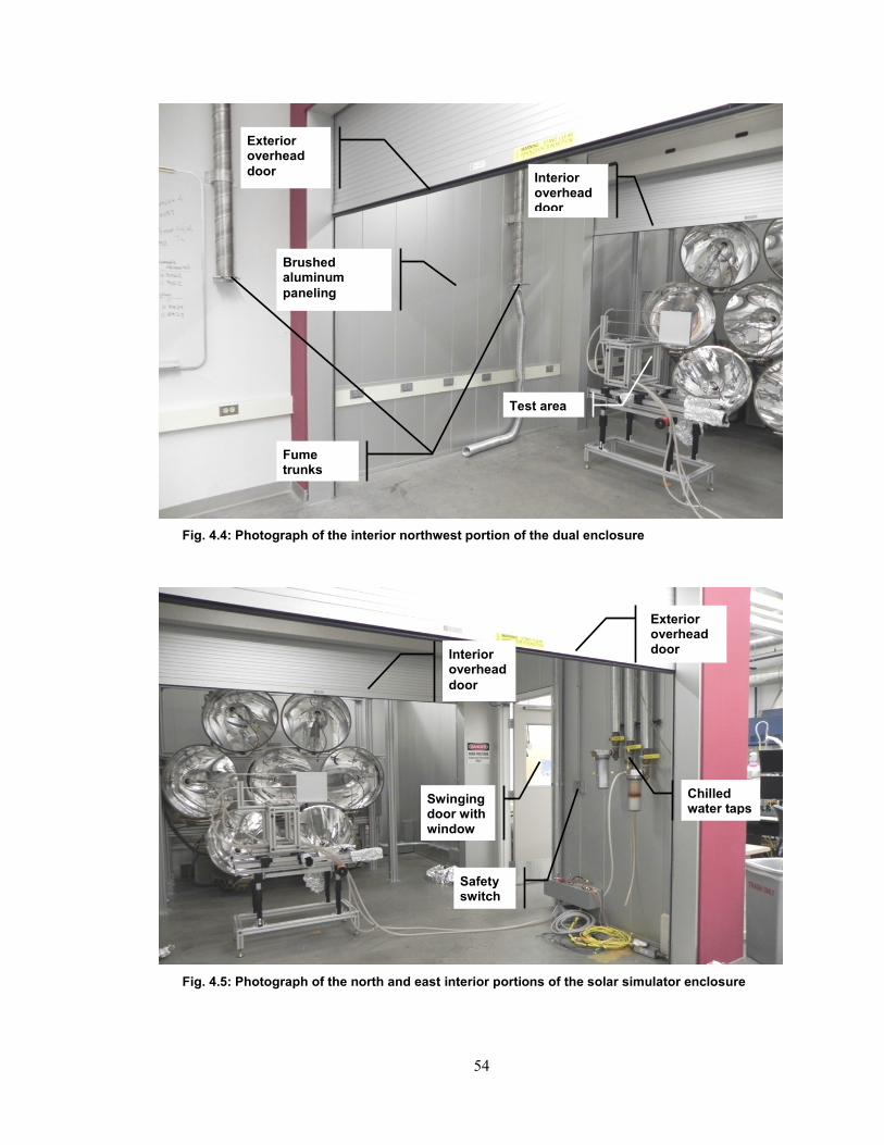
54

Fig. 4.4: Photograph of the interior northwest portion of the dual enclosure

Fig. 4.5: Photograph of the north and east interior portions of the solar simulator enclosure

Exterior overhead

door Interior overhead door

Fume trunks

Test area

Interior overhead

door

Exterior overhead door

Chilled water taps

Safety switch

Swinging door with window

Brushed aluminum

paneling

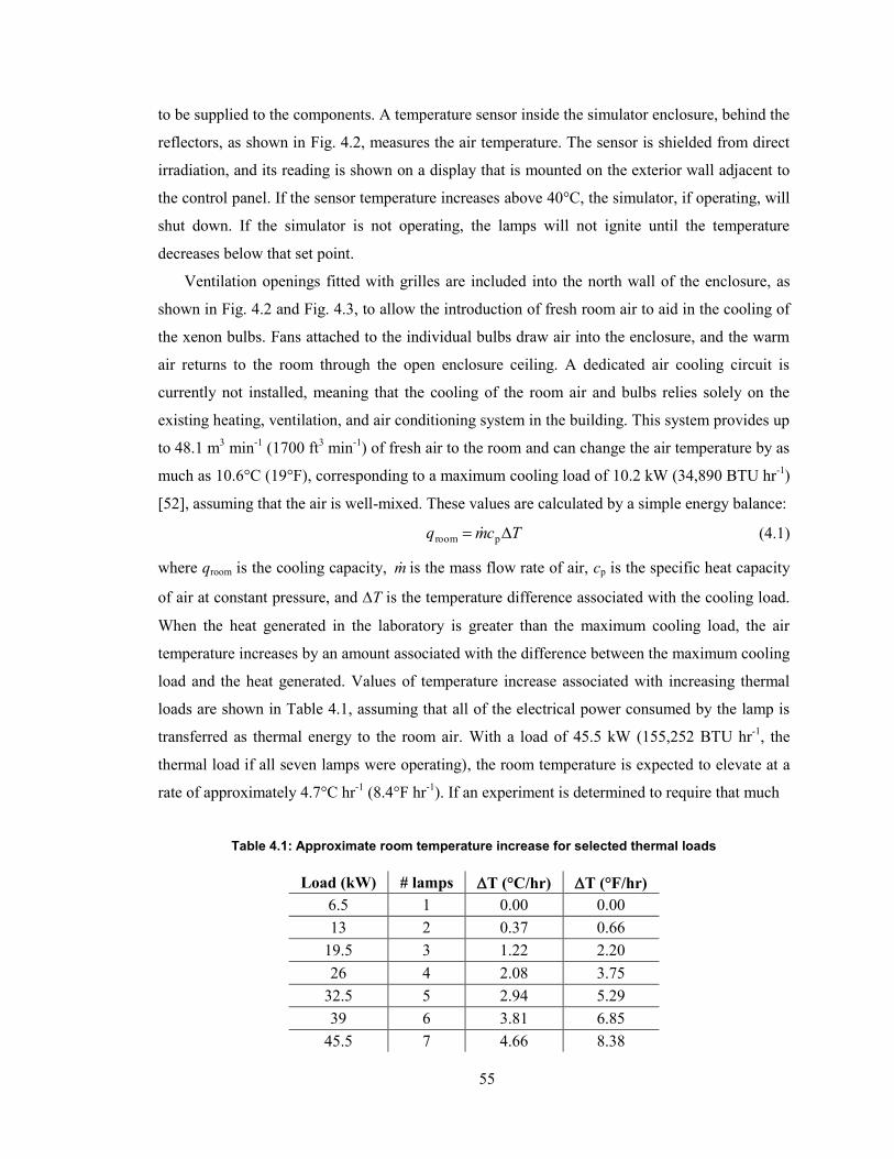
55

to be supplied to the components. A temperature sensor inside the simulator enclosure, behind the

reflectors, as shown in Fig. 4.2, measures the air temperature. The sensor is shielded from direct

irradiation, and its reading is shown on a display that is mounted on the exterior wall adjacent to

the control panel. If the sensor temperature increases above 40°C, the simulator, if operating, will

shut down. If the simulator is not operating, the lamps will not ignite until the temperature

decreases below that set point.

Ventilation openings fitted with grilles are included into the north wall of the enclosure, as

shown in Fig. 4.2 and Fig. 4.3, to allow the introduction of fresh room air to aid in the cooling of

the xenon bulbs. Fans attached to the individual bulbs draw air into the enclosure, and the warm

air returns to the room through the open enclosure ceiling. A dedicated air cooling circuit is

currently not installed, meaning that the cooling of the room air and bulbs relies solely on the

existing heating, ventilation, and air conditioning system in the building. This system provides up

to 48.1 m3 min

-1 (1700 ft

3 min

-1) of fresh air to the room and can change the air temperature by as

much as 10.6°C (19°F), corresponding to a maximum cooling load of 10.2 kW (34,890 BTU hr-1

)

[52], assuming that the air is well-mixed. These values are calculated by a simple energy balance:

Tcmq proom (4.1)

where qroom is the cooling capacity, m is the mass flow rate of air, cp is the specific heat capacity

of air at constant pressure, and T is the temperature difference associated with the cooling load.

When the heat generated in the laboratory is greater than the maximum cooling load, the air

temperature increases by an amount associated with the difference between the maximum cooling

load and the heat generated. Values of temperature increase associated with increasing thermal

loads are shown in Table 4.1, assuming that all of the electrical power consumed by the lamp is

transferred as thermal energy to the room air. With a load of 45.5 kW (155,252 BTU hr-1

, the

thermal load if all seven lamps were operating), the room temperature is expected to elevate at a

rate of approximately 4.7°C hr-1

(8.4°F hr-1

). If an experiment is determined to require that much

Table 4.1: Approximate room temperature increase for selected thermal loads

Load (kW) # lamps T (°C/hr) T (°F/hr)

6.5 1 0.00 0.00

13 2 0.37 0.66

19.5 3 1.22 2.20

26 4 2.08 3.75

32.5 5 2.94 5.29

39 6 3.81 6.85

45.5 7 4.66 8.38

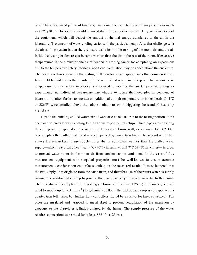
56

power for an extended period of time, e.g., six hours, the room temperature may rise by as much

as 28°C (50°F). However, it should be noted that many experiments will likely use water to cool

the equipment, which will deduct the amount of thermal energy transferred to the air in the

laboratory. The amount of water cooling varies with the particular setup. A further challenge with

the air cooling system is that the enclosure walls inhibit the mixing of the room air, and the air

inside the testing enclosure can become warmer than the air in the rest of the room. If excessive

temperatures in the simulator enclosure become a limiting factor for completing an experiment

due to the temperature safety interlock, additional ventilation may be added above the enclosure.

The beam structures spanning the ceiling of the enclosure are spaced such that commercial box

fans could be laid across them, aiding in the removal of warm air. The probe that measures air

temperature for the safety interlocks is also used to monitor the air temperature during an

experiment, and individual researchers may choose to locate thermocouples in positions of

interest to monitor further temperatures. Additionally, high-temperature sprinkler heads (141°C

or 286°F) were installed above the solar simulator to avoid triggering the standard heads by

heated air.

Taps to the building chilled water circuit were also added and run to the testing portion of the

enclosure to provide water cooling to the various experimental setups. Three pipes are run along

the ceiling and dropped along the interior of the east enclosure wall, as shown in Fig. 4.2. One

pipe supplies the chilled water and is accompanied by two return lines. The second return line

allows the researchers to use supply water that is somewhat warmer than the chilled water

supply—which is typically kept near 4°C (40°F) in summer and 7°C (44°F) in winter— in order

to prevent water vapor in the room air from condensing on equipment. In the case of flux

measurement equipment whose optical properties must be well-known to ensure accurate

measurements, condensation on surfaces could alter the measured results. It must be noted that

the two supply lines originate from the same main, and therefore use of the return water as supply

requires the addition of a pump to provide the head necessary to return the water to the mains.

The pipe diameters supplied to the testing enclosure are 32 mm (1.25 in) in diameter, and are

rated to supply up to 56.8 l min-1

(15 gal min-1

) of flow. The end of each drop is equipped with a

quarter turn ball valve, but further flow controllers should be installed for finer adjustment. The

pipes are insulated and wrapped in metal sheet to prevent degradation of the insulation by

exposure to the ultraviolet radiation emitted by the lamps. The supply pressure of the water

requires connections to be rated for at least 862 kPa (125 psi).

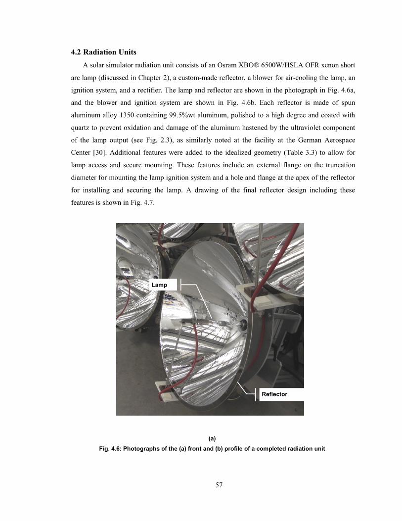
57

4.2 Radiation Units

A solar simulator radiation unit consists of an Osram XBO® 6500W/HSLA OFR xenon short

arc lamp (discussed in Chapter 2), a custom-made reflector, a blower for air-cooling the lamp, an

ignition system, and a rectifier. The lamp and reflector are shown in the photograph in Fig. 4.6a,

and the blower and ignition system are shown in Fig. 4.6b. Each reflector is made of spun

aluminum alloy 1350 containing 99.5%wt aluminum, polished to a high degree and coated with

quartz to prevent oxidation and damage of the aluminum hastened by the ultraviolet component

of the lamp output (see Fig. 2.3), as similarly noted at the facility at the German Aerospace

Center [30]. Additional features were added to the idealized geometry (Table 3.3) to allow for

lamp access and secure mounting. These features include an external flange on the truncation

diameter for mounting the lamp ignition system and a hole and flange at the apex of the reflector

for installing and securing the lamp. A drawing of the final reflector design including these

features is shown in Fig. 4.7.

(a)

Fig. 4.6: Photographs of the (a) front and (b) profile of a completed radiation unit

Lamp

Reflector

58

(b)

Fig. 4.6 (cont.): Photographs of the (a) front and (b) profile of a completed radiation unit

Fig. 4.7: Cross-sectional drawing of the final reflector geometry, including mounting flanges and lamp access hole. All dimensions are in mm. Image provided by Kinoton, GmbH

Blower

Ignition

system

Flat mounting

plate for blower,

lamp, and

electronics

Reflector

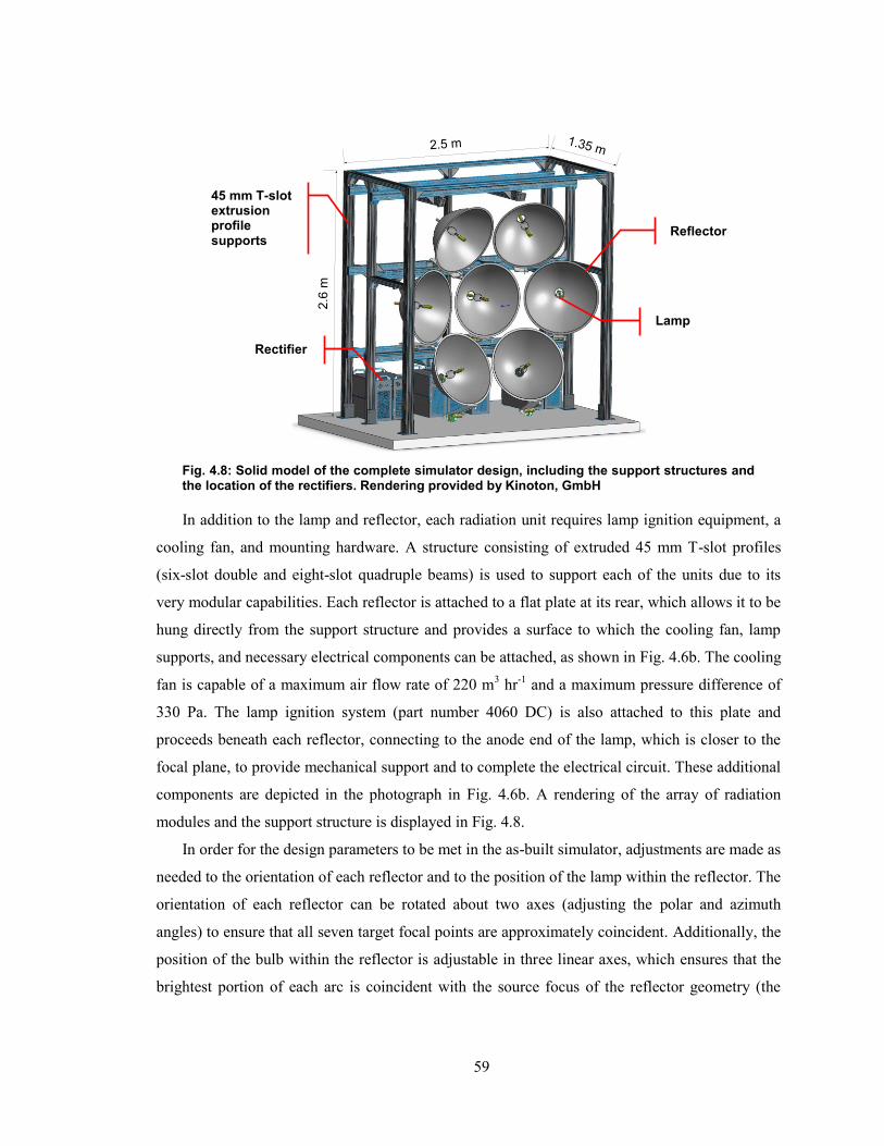
59

Fig. 4.8: Solid model of the complete simulator design, including the support structures and the location of the rectifiers. Rendering provided by Kinoton, GmbH

In addition to the lamp and reflector, each radiation unit requires lamp ignition equipment, a

cooling fan, and mounting hardware. A structure consisting of extruded 45 mm T-slot profiles

(six-slot double and eight-slot quadruple beams) is used to support each of the units due to its

very modular capabilities. Each reflector is attached to a flat plate at its rear, which allows it to be

hung directly from the support structure and provides a surface to which the cooling fan, lamp

supports, and necessary electrical components can be attached, as shown in Fig. 4.6b. The cooling

fan is capable of a maximum air flow rate of 220 m3 hr

-1 and a maximum pressure difference of

330 Pa. The lamp ignition system (part number 4060 DC) is also attached to this plate and

proceeds beneath each reflector, connecting to the anode end of the lamp, which is closer to the

focal plane, to provide mechanical support and to complete the electrical circuit. These additional

components are depicted in the photograph in Fig. 4.6b. A rendering of the array of radiation

modules and the support structure is displayed in Fig. 4.8.

In order for the design parameters to be met in the as-built simulator, adjustments are made as

needed to the orientation of each reflector and to the position of the lamp within the reflector. The

orientation of each reflector can be rotated about two axes (adjusting the polar and azimuth

angles) to ensure that all seven target focal points are approximately coincident. Additionally, the

position of the bulb within the reflector is adjustable in three linear axes, which ensures that the

brightest portion of each arc is coincident with the source focus of the reflector geometry (the

2.6

m

2.5 m 1.35 m

Reflector

Lamp

Rectifier

45 mm T-slot extrusion profile supports

60

optimal position for concentrating the lamp output). A detailed description of the procedure for

adjusting these orientations and locations is in Appendix B.

Each lamp draws up to 6500 W (170 A of DC current and 38 V) during steady state

operation. The input current is specified by the user in the control software and is variable in the

range of 140–175 A (currents above 170A are considered overdriven), and the voltage is

automatically adjusted to maintain that current [51]. Current adjustments in this range are used to

fine-tune the amount of radiative power output by each unit. Each lamp requires 40 VDC for

ignition. This high DC power is supplied by rectifiers that are connected to AC mains power,

which, in this case, is provided by a dedicated transformer located in room 1134A. Renderings of

the rectifiers are shown in Fig. 4.8.

Due to their previous experience constructing a solar simulator with a similar concept for the

German Aerospace Institute [30], Kinoton GmbH was contracted to construct and finalize the

design of the mechanical and electrical components for the UMN solar simulator. A complete

users’ manual for operating the solar simulator is presented in Appendix C. The final solar

simulator, its support structure, dedicated enclosure, power and control electronics, and flux

measurement equipment was constructed and functioning in the first week of December, 2010.

The solar simulator facility is also outfitted with equipment that is used to measure and calibrate

its radiative flux output. Further details on these calibration and measurement methods, as well as

the instrumentation, are provided in Chapter 5.

4.3 Summary

The solar simulator was installed and functioning by December 2010 at the University of

Minnesota. A dedicated enclosure was constructed within Mechanical Engineering room 1134 to

house and protect the simulator and shield researchers from its extreme radiative output, and it is

equipped with chilled water and air cooling systems. The reflectors were constructed of spun and

polished aluminum alloy 1350, which consists of 99.5% aluminum, and were coated with quartz

to prevent degradation and corrosion. The electrical power supplied to each lamp can be adjusted

to fine-tune the radiative output of each lamp, and many precautions are hard-wired to the

controls to ensure safe operation. Specialized equipment to measure concentrated radiative flux is

also provided; details are described in Chapter 5.

61

Chapter 5

Measurement and Calibration Techniques

Accurate measurement of the solar simulator’s radiative output is imperative in evaluating the

performance of prototype receivers and reactors. A common benchmark calculation in

determining reactor performance is its efficiency, usually defined as the useful work output

divided by the energy input, which is provided by the solar simulator. For this reason, the

radiative flux is measured with as much accuracy as possible using an optical technique that is

commonly used in concentrating solar facilities. Measured flux distributions for solar dish

facilities have reported uncertainty values in radiative power of ±2–4% [14,53]; an uncertainty of

±3% or less of the radiative power measurements is sought in this study. The method used to

obtain these flux measurements involves locating a water-cooled Lambertian target in the

measurement plane, while a CCD camera views the target through absorptive-reflective neutral

density filters and a lens. The grayscale photograph output by the camera is calibrated by directly

measuring the incident flux and relating it to the average grayscale level in the same region. This

calibration is completed with a circular foil heat flux gage that must be calibrated in-house for use

in concentrated xenon radiation due to the different spectral distribution compared to the radiation

source used in the gage manufacturer’s calibration. The circular foil heat flux gage is treated as a

calorimeter in this calibration, and the incident radiative flux is determined from a heat transfer

model including energy transfer from the gage to the cooling water and by conduction heat

transfer between the gage and the target in which it is embedded. Convection and reradiation

between the gage and the surroundings are negligible.

5.1 Measurement Method & Instrumentation

The radiative flux output of the simulator is measured optically by viewing the radiation

reflected from a diffusely-reflecting Lambertian target with a charge coupled device (CCD)

camera equipped with neutral density filters and a lens, shown schematically in Fig. 5.1. The

grayscale values output by the camera are calibrated to measured levels of radiative flux by

measuring the incident flux with a circular foil heat flux gage.

The optical measurement system consists of a 12-bit 1392×1040 pixel Basler Scout scA

1400-17gm CCD camera, two stacked CVI Melles-Griot NDQ-400 reflective-absorptive neutral

density filters, a Pentax C22516TH 25mm F1.8 lens, and two 250-mm-square Lambertian targets.

The F-number of the lens and the neutral density filters are selected such that the pixel with the

greatest exposure has a grayscale value approximately 70–80% of the full bit depth of the camera.

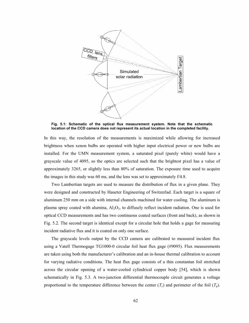
62

Fig. 5.1: Schematic of the optical flux measurement system. Note that the schematic location of the CCD camera does not represent its actual location in the completed facility.

In this way, the resolution of the measurements is maximized while allowing for increased

brightness when xenon bulbs are operated with higher input electrical power or new bulbs are

installed. For the UMN measurement system, a saturated pixel (purely white) would have a

grayscale value of 4095, so the optics are selected such that the brightest pixel has a value of

approximately 3265, or slightly less than 80% of saturation. The exposure time used to acquire

the images in this study was 60 ms, and the lens was set to approximately f/4.8.

Two Lambertian targets are used to measure the distribution of flux in a given plane. They

were designed and constructed by Haueter Engineering of Switzerlad. Each target is a square of

aluminum 250 mm on a side with internal channels machined for water cooling. The aluminum is

plasma spray coated with alumina, Al2O3, to diffusely reflect incident radiation. One is used for

optical CCD measurements and has two continuous coated surfaces (front and back), as shown in

Fig. 5.2. The second target is identical except for a circular hole that holds a gage for measuring

incident radiative flux and it is coated on only one surface.

The grayscale levels output by the CCD camera are calibrated to measured incident flux

using a Vatell Thermogage TG1000-0 circular foil heat flux gage (#9095). Flux measurements

are taken using both the manufacturer’s calibration and an in-house thermal calibration to account

for varying radiative conditions. The heat flux gage consists of a thin constantan foil stretched

across the circular opening of a water-cooled cylindrical copper body [54], which is shown

schematically in Fig. 5.3. A two-junction differential thermocouple circuit generates a voltage

proportional to the temperature difference between the center (Tc) and perimeter of the foil (Tp).

63

Fig. 5.2: Photograph of the Lambertian target without a hole, mounted for flux measurement

Fig. 5.3: Schematic cross-section of a circular foil heat flux gage

The center junction is formed by a thin copper wire attached to the center of the constantan foil,

while the edge junction is formed by the connection of the constantan foil to the copper body

around the entire perimeter. The diameter and thickness of the foil vary for the calibration

required by each instrument. The foil is thin enough that, although its diameter is very small (only

1.016 mm (0.04 in) for the current gage), the voltage due to the temperature difference occurring

between the center and edge is measurable without amplification. The diameter of the gage body

is 25.3 mm (0.995 in). The emf generated by the thermocouple circuit is 0–10 mV, indicating that

a temperature difference of up to approximately 213°C is possible in the foil, as determined from

the published calibration tables for type T thermocouples.

The gage is calibrated by the manufacturer with a two-step process employing a reference

gage that has an absorptive coating identical to the commercially sold gage (colloidal graphite for

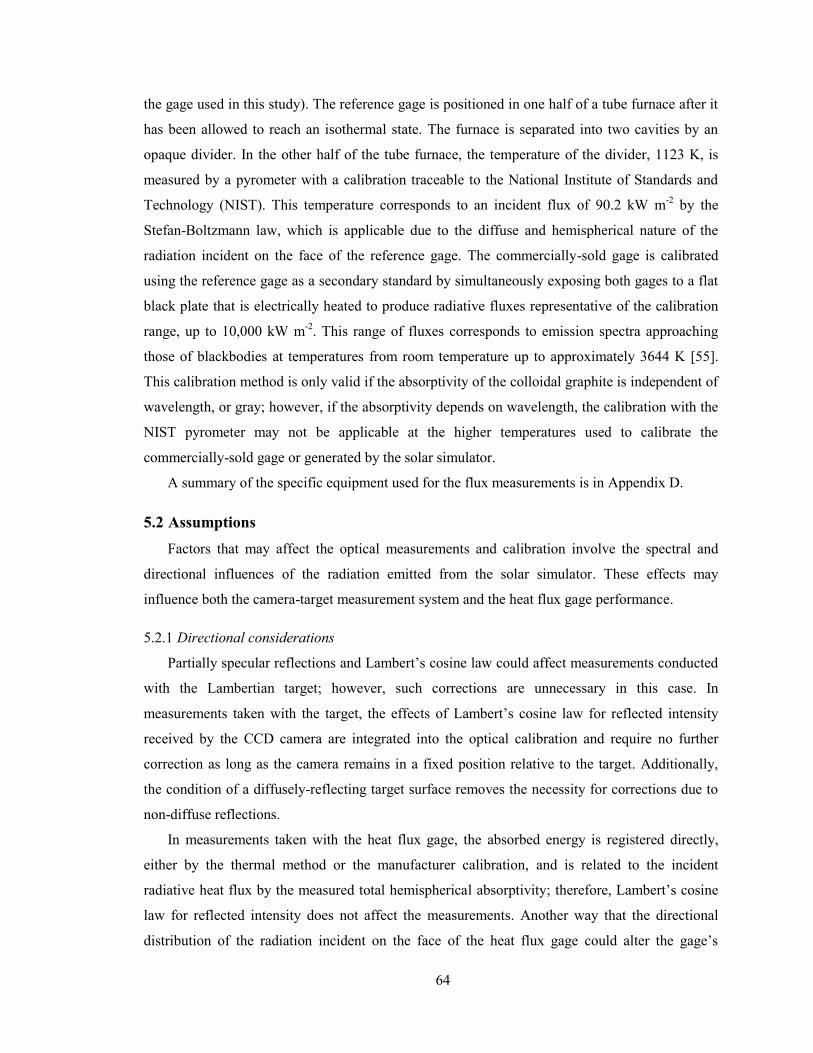
64

the gage used in this study). The reference gage is positioned in one half of a tube furnace after it

has been allowed to reach an isothermal state. The furnace is separated into two cavities by an

opaque divider. In the other half of the tube furnace, the temperature of the divider, 1123 K, is

measured by a pyrometer with a calibration traceable to the National Institute of Standards and

Technology (NIST). This temperature corresponds to an incident flux of 90.2 kW m-2

by the

Stefan-Boltzmann law, which is applicable due to the diffuse and hemispherical nature of the

radiation incident on the face of the reference gage. The commercially-sold gage is calibrated

using the reference gage as a secondary standard by simultaneously exposing both gages to a flat

black plate that is electrically heated to produce radiative fluxes representative of the calibration

range, up to 10,000 kW m-2

. This range of fluxes corresponds to emission spectra approaching

those of blackbodies at temperatures from room temperature up to approximately 3644 K [55].

This calibration method is only valid if the absorptivity of the colloidal graphite is independent of

wavelength, or gray; however, if the absorptivity depends on wavelength, the calibration with the

NIST pyrometer may not be applicable at the higher temperatures used to calibrate the

commercially-sold gage or generated by the solar simulator.

A summary of the specific equipment used for the flux measurements is in Appendix D.

5.2 Assumptions

Factors that may affect the optical measurements and calibration involve the spectral and

directional influences of the radiation emitted from the solar simulator. These effects may

influence both the camera-target measurement system and the heat flux gage performance.

5.2.1 Directional considerations

Partially specular reflections and Lambert’s cosine law could affect measurements conducted

with the Lambertian target; however, such corrections are unnecessary in this case. In

measurements taken with the target, the effects of Lambert’s cosine law for reflected intensity

received by the CCD camera are integrated into the optical calibration and require no further

correction as long as the camera remains in a fixed position relative to the target. Additionally,

the condition of a diffusely-reflecting target surface removes the necessity for corrections due to

non-diffuse reflections.

In measurements taken with the heat flux gage, the absorbed energy is registered directly,

either by the thermal method or the manufacturer calibration, and is related to the incident

radiative heat flux by the measured total hemispherical absorptivity; therefore, Lambert’s cosine

law for reflected intensity does not affect the measurements. Another way that the directional

distribution of the radiation incident on the face of the heat flux gage could alter the gage’s

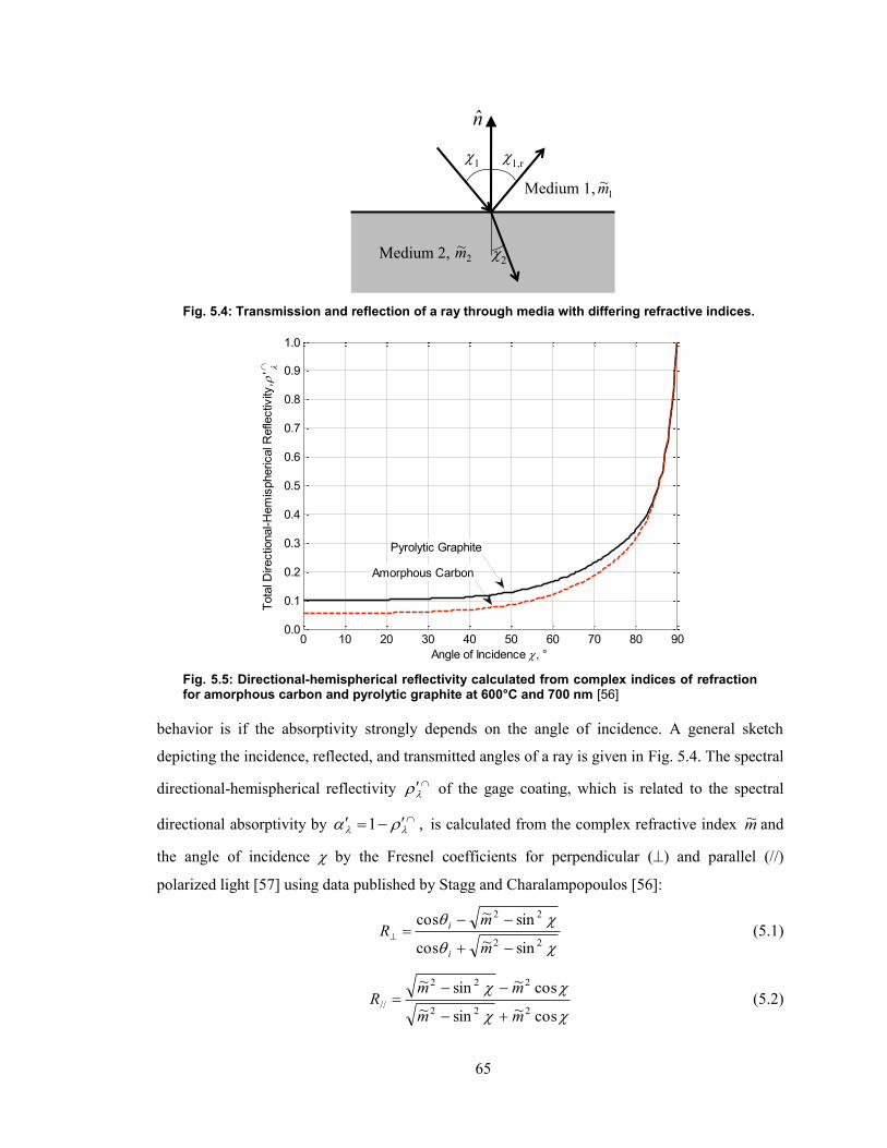
65

Fig. 5.4: Transmission and reflection of a ray through media with differing refractive indices.

Fig. 5.5: Directional-hemispherical reflectivity calculated from complex indices of refraction for amorphous carbon and pyrolytic graphite at 600°C and 700 nm [56]

behavior is if the absorptivity strongly depends on the angle of incidence. A general sketch

depicting the incidence, reflected, and transmitted angles of a ray is given in Fig. 5.4. The spectral

directional-hemispherical reflectivity of the gage coating, which is related to the spectral

directional absorptivity by ,1 is calculated from the complex refractive index m~ and

the angle of incidence by the Fresnel coefficients for perpendicular () and parallel (//)

polarized light [57] using data published by Stagg and Charalampopoulos [56]:

22

22

sin~cos

sin~cos

m

mR

i

i

(5.1)

cos~sin~

cos~sin~

222

222

//

mm

mmR

(5.2)

Medium 1,

Medium 2,

1

2

n

1,r

2~m

1~m

0 10 20 30 40 50 60 70 80 900.0

0.1

0.2

0.3

0.4

0.5

0.6

0.7

0.8

0.9

1.0

Angle of Incidence , °

Tota

l Directio

nal-H

em

ispherical R

efle

ctiv

ity,

'

600°C and 700 nm

Pyrolytic Graphite

Amorphous Carbon

66

2

//

2

21 RR

(5.3)

Values of vary almost imperceptibly in the temperature and wavelength ranges studied

(25–600°C and 400–700 nm) for the refractive indices of both amorphous carbon and pyrolytic

graphite [56], so representative curves for each material at 600°C and 700 nm are shown in Fig.

5.5. Both materials show constant values of reflectivity for incidence angles less than

approximately 40°. Because the simulator rim angle rim, as determined in Chapter 2, is

approximately 38°, it is expected that the majority of the radiation contacts the heat flux gage

with ≤ 38°; therefore, the directional dependence of the absorptivity of the heat flux gage

coating is not expected to significantly affect the behavior of the heat flux gage.

5.2.2 Spectral considerations

The optical measurement method requires the assumption that the solar simulator emission

spectrum remains constant over time and throughout the spatial radiative flux distribution because

the spectral sensitivities of the filters, lens, and CCD camera are incorporated into the calibration.

Spatially-varying spectra such as those presented by Alxneit and Schmit [58], if present in the

UMN solar simulator, may require further corrections to measured data. The spectral intensity

output by the ten-lamp solar simulator at the Paul Scherrer Institut (PSI) was measured at various

locations in the focal plane. These spectral distributions were compared in terms of the relative

amounts of energy contributed in different wavelength ranges. It was found that the xenon

emission lines between approximately 800–1000 nm (see Fig. 2.3) comprise an increasing portion

of the total energy with increasing radius from the distribution center, whereas the relative

contribution of energy in the ultraviolet (UV) wavelengths decreases with increasing radius. As

an example, spectral measurements taken at 880 nm using all ten lamps at a radius of 50 mm

contain approximately 1.6 times more energy than spectra measured at the center of the

distribution. Furthermore, at 350 nm, 5% less energy was measured in the spectrum at a 50 mm

radius than the spectrum measured at the center. These measurements had a repeatability of 15%

[58]. The spatial variations in spectrum are expected to be caused by different regions of the

plasma arc emitting with different spectral distributions, as shown by Nakar et al. [59]. Spectra

emitted from varying points within the arc volume are mapped to different locations in the focal

plane, corresponding to their emission points.

The CCD cameras, lenses, and optical filters used to measure concentrated flux, both at PSI

and UMN, each have spectral sensitivities or transmittances. If the spectrum in the focal plane

was equal at all locations, these spectral variations would be incorporated into the flux

calibration; however, if the spectral distribution of flux varies with location, then the calibration

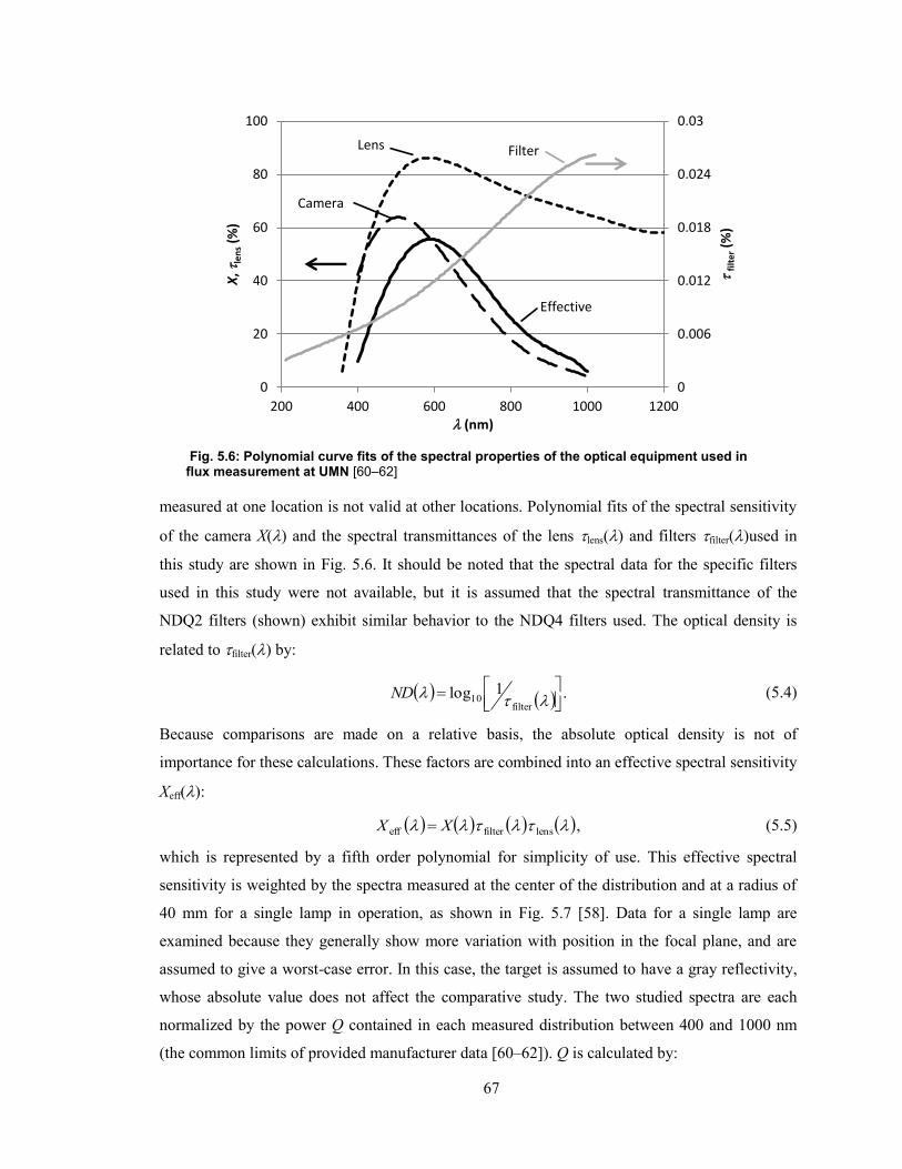
67

Fig. 5.6: Polynomial curve fits of the spectral properties of the optical equipment used in flux measurement at UMN [60–62]

measured at one location is not valid at other locations. Polynomial fits of the spectral sensitivity

of the camera X() and the spectral transmittances of the lens lens() and filters filter()used in

this study are shown in Fig. 5.6. It should be noted that the spectral data for the specific filters

used in this study were not available, but it is assumed that the spectral transmittance of the

NDQ2 filters (shown) exhibit similar behavior to the NDQ4 filters used. The optical density is

related to filter() by:

.1logfilter

10

ND

(5.4)

Because comparisons are made on a relative basis, the absolute optical density is not of

importance for these calculations. These factors are combined into an effective spectral sensitivity

Xeff():

,lensfiltereff XX

(5.5)

which is represented by a fifth order polynomial for simplicity of use. This effective spectral

sensitivity is weighted by the spectra measured at the center of the distribution and at a radius of

40 mm for a single lamp in operation, as shown in Fig. 5.7 [58]. Data for a single lamp are

examined because they generally show more variation with position in the focal plane, and are

assumed to give a worst-case error. In this case, the target is assumed to have a gray reflectivity,

whose absolute value does not affect the comparative study. The two studied spectra are each

normalized by the power Q contained in each measured distribution between 400 and 1000 nm

(the common limits of provided manufacturer data [60–62]). Q is calculated by:

0

0.006

0.012

0.018

0.024

0.03

0

20

40

60

80

100

200 400 600 800 1000 1200

fi

lte

r (%

)

X,

len

s (%

)

(nm)

Lens Filter

Camera

Effective

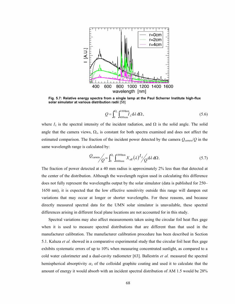
68

Fig. 5.7: Relative energy spectra from a single lamp at the Paul Scherrer Institute high-flux solar simulator at various distribution radii [58]

,dd0

nm1000

400nm

i

IQ

(5.6)

where I is the spectral intensity of the incident radiation, and is the solid angle. The solid

angle that the camera views, i, is constant for both spectra examined and does not affect the

estimated comparison. The fraction of the incident power detected by the camera Qcamera/Q in the

same wavelength range is calculated by:

.dd0

nm1000

400nmeff

camera

i

QI

XQ

Q

(5.7)

The fraction of power detected at a 40 mm radius is approximately 2% less than that detected at

the center of the distribution. Although the wavelength region used in calculating this difference

does not fully represent the wavelengths output by the solar simulator (data is published for 250–

1650 nm), it is expected that the low effective sensitivity outside this range will dampen out

variations that may occur at longer or shorter wavelengths. For these reasons, and because

directly measured spectral data for the UMN solar simulator is unavailable, these spectral

differences arising in different focal plane locations are not accounted for in this study.

Spectral variations may also affect measurements taken using the circular foil heat flux gage

when it is used to measure spectral distributions that are different than that used in the

manufacturer calibration. The manufacturer calibration procedure has been described in Section

5.1. Kaluza et al. showed in a comparative experimental study that the circular foil heat flux gage

exhibits systematic errors of up to 10% when measuring concentrated sunlight, as compared to a

cold water calorimeter and a dual-cavity radiometer [63]. Ballestrín et al. measured the spectral

hemispherical absorptivity of the colloidal graphite coating and used it to calculate that the

amount of energy it would absorb with an incident spectral distribution of AM 1.5 would be 28%

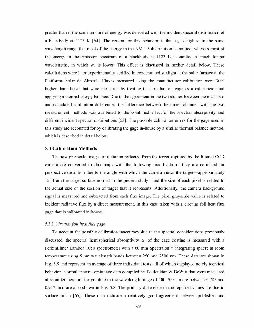
69

greater than if the same amount of energy was delivered with the incident spectral distribution of

a blackbody at 1123 K [64]. The reason for this behavior is that is highest in the same

wavelength range that most of the energy in the AM 1.5 distribution is emitted, whereas most of

the energy in the emission spectrum of a blackbody at 1123 K is emitted at much longer

wavelengths, in which is lower. This effect is discussed in further detail below. These

calculations were later experimentally verified in concentrated sunlight at the solar furnace at the

Platforma Solar de Almería. Fluxes measured using the manufacturer calibration were 30%

higher than fluxes that were measured by treating the circular foil gage as a calorimeter and

applying a thermal energy balance. Due to the agreement in the two studies between the measured

and calculated calibration differences, the difference between the fluxes obtained with the two

measurement methods was attributed to the combined effect of the spectral absorptivity and

different incident spectral distributions [53]. The possible calibration errors for the gage used in

this study are accounted for by calibrating the gage in-house by a similar thermal balance method,

which is described in detail below.

5.3 Calibration Methods

The raw grayscale images of radiation reflected from the target captured by the filtered CCD

camera are converted to flux maps with the following modifications: they are corrected for

perspective distortion due to the angle with which the camera views the target—approximately

15° from the target surface normal in the present study—and the size of each pixel is related to

the actual size of the section of target that it represents. Additionally, the camera background

signal is measured and subtracted from each flux image. The pixel grayscale value is related to

incident radiative flux by a direct measurement, in this case taken with a circular foil heat flux

gage that is calibrated in-house.

5.3.1 Circular foil heat flux gage

To account for possible calibration inaccuracy due to the spectral considerations previously

discussed, the spectral hemispherical absorptivity of the gage coating is measured with a

PerkinElmer Lambda 1050 spectrometer with a 60 mm Spectralon™ integrating sphere at room

temperature using 5 nm wavelength bands between 250 and 2500 nm. These data are shown in

Fig. 5.8 and represent an average of three individual tests, all of which displayed nearly identical

behavior. Normal spectral emittance data compiled by Touloukian & DeWitt that were measured

at room temperature for graphite in the wavelength range of 400-700 nm are between 0.785 and

0.937, and are also shown in Fig. 5.8. The primary difference in the reported values are due to

surface finish [65]. These data indicate a relatively good agreement between published and

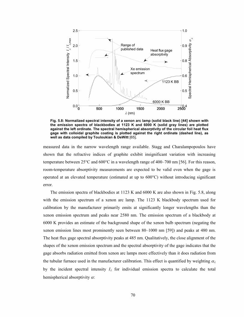
70

Fig. 5.8: Normalized spectral intensity of a xenon arc lamp (solid black line) [44] shown with the emission spectra of blackbodies at 1123 K and 6000 K (solid gray lines) are plotted against the left ordinate. The spectral hemispherical absorptivity of the circular foil heat flux gage with colloidal graphite coating is plotted against the right ordinate (dashed line), as well as data compiled by Touloukian & DeWitt [65].

measured data in the narrow wavelength range available. Stagg and Charalampopoulos have

shown that the refractive indices of graphite exhibit insignificant variation with increasing

temperature between 25°C and 600°C in a wavelength range of 400–700 nm [56]. For this reason,

room-temperature absorptivity measurements are expected to be valid even when the gage is

operated at an elevated temperature (estimated at up to 600°C) without introducing significant

error.

The emission spectra of blackbodies at 1123 K and 6000 K are also shown in Fig. 5.8, along

with the emission spectrum of a xenon arc lamp. The 1123 K blackbody spectrum used for

calibration by the manufacturer primarily emits at significantly longer wavelengths than the

xenon emission spectrum and peaks near 2580 nm. The emission spectrum of a blackbody at

6000 K provides an estimate of the background shape of the xenon bulb spectrum (negating the

xenon emission lines most prominently seen between 80–1000 nm [59]) and peaks at 480 nm.

The heat flux gage spectral absorptivity peaks at 485 nm. Qualitatively, the close alignment of the

shapes of the xenon emission spectrum and the spectral absorptivity of the gage indicates that the

gage absorbs radiation emitted from xenon arc lamps more effectively than it does radiation from

the tubular furnace used in the manufacturer calibration. This effect is quantified by weighting

by the incident spectral intensity I for individual emission spectra to calculate the total

hemispherical absorptivity :

0 500 1000 1500 2000 25000.0

0.5

1.0

1.5

2.0

2.5

No

rma

lize

d S

pe

ctr

al In

ten

sity I

/ I,m

ax

0 500 1000 1500 2000 25000.4

0.5

0.6

0.8

0.9

1.0

Sp

ectr

al H

em

isp

he

rica

l A

bso

rptivity

(nm)

1123 K BB

6000 K BB

Range of published data Heat flux gage

absorptivity

Xe emissionspectrum

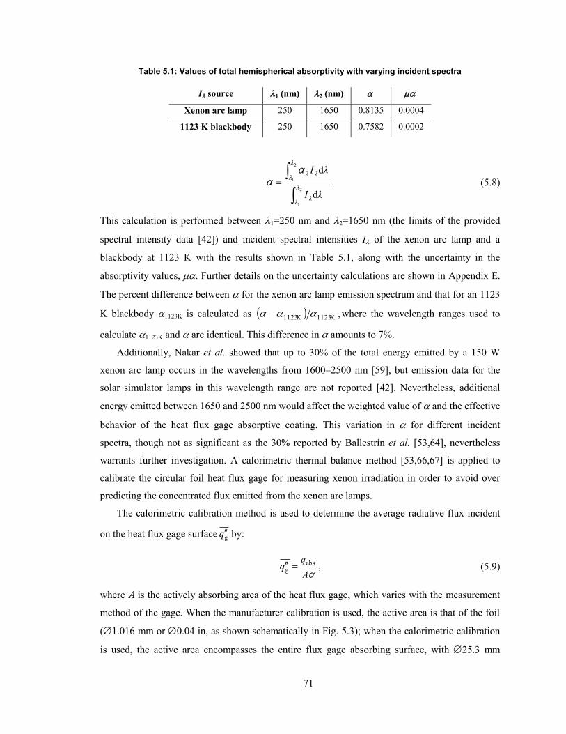
71

Table 5.1: Values of total hemispherical absorptivity with varying incident spectra

I source 1 (nm) 2 (nm)

Xenon arc lamp 250 1650 0.8135 0.0004

1123 K blackbody 250 1650 0.7582 0.0002

.

d

d

2

1

2

1

λI

λI

λ

λλαα

(5.8)

This calculation is performed between 1=250 nm and 2=1650 nm (the limits of the provided

spectral intensity data [42]) and incident spectral intensities I of the xenon arc lamp and a

blackbody at 1123 K with the results shown in Table 5.1, along with the uncertainty in the

absorptivity values, . Further details on the uncertainty calculations are shown in Appendix E.

The percent difference between for the xenon arc lamp emission spectrum and that for an 1123

K blackbody 1123K is calculated as ,K1123K1123 where the wavelength ranges used to

calculate 1123K and are identical. This difference in amounts to 7%.

Additionally, Nakar et al. showed that up to 30% of the total energy emitted by a 150 W

xenon arc lamp occurs in the wavelengths from 1600–2500 nm [59], but emission data for the

solar simulator lamps in this wavelength range are not reported [42]. Nevertheless, additional

energy emitted between 1650 and 2500 nm would affect the weighted value of and the effective

behavior of the heat flux gage absorptive coating. This variation in for different incident

spectra, though not as significant as the 30% reported by Ballestrín et al. [53,64], nevertheless

warrants further investigation. A calorimetric thermal balance method [53,66,67] is applied to

calibrate the circular foil heat flux gage for measuring xenon irradiation in order to avoid over

predicting the concentrated flux emitted from the xenon arc lamps.

The calorimetric calibration method is used to determine the average radiative flux incident

on the heat flux gage surface gq by:

,abs

gαA

qq

(5.9)

where A is the actively absorbing area of the heat flux gage, which varies with the measurement

method of the gage. When the manufacturer calibration is used, the active area is that of the foil

(1.016 mm or 0.04 in, as shown schematically in Fig. 5.3); when the calorimetric calibration

is used, the active area encompasses the entire flux gage absorbing surface, with 25.3 mm

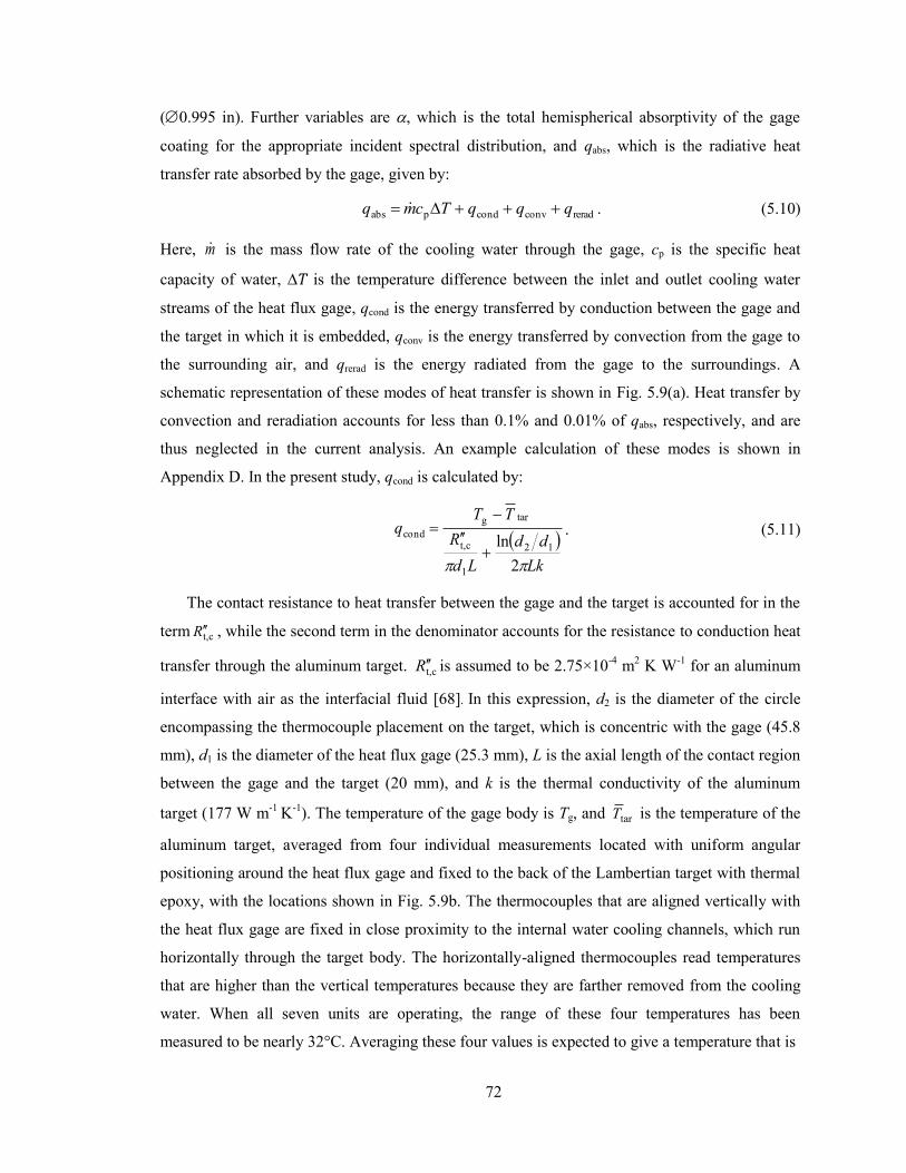
72

(0.995 in). Further variables are , which is the total hemispherical absorptivity of the gage

coating for the appropriate incident spectral distribution, and qabs, which is the radiative heat

transfer rate absorbed by the gage, given by:

reradconvcondpabs qqqTcmq . (5.10)

Here, m is the mass flow rate of the cooling water through the gage, cp is the specific heat

capacity of water, T is the temperature difference between the inlet and outlet cooling water

streams of the heat flux gage, qcond is the energy transferred by conduction between the gage and

the target in which it is embedded, qconv is the energy transferred by convection from the gage to

the surrounding air, and qrerad is the energy radiated from the gage to the surroundings. A

schematic representation of these modes of heat transfer is shown in Fig. 5.9(a). Heat transfer by

convection and reradiation accounts for less than 0.1% and 0.01% of qabs, respectively, and are

thus neglected in the current analysis. An example calculation of these modes is shown in

Appendix D. In the present study, qcond is calculated by:

Lk

dd

Ld

R

TTq

2

ln 12

1

ct,

targ

cond

. (5.11)

The contact resistance to heat transfer between the gage and the target is accounted for in the

term ct,R , while the second term in the denominator accounts for the resistance to conduction heat

transfer through the aluminum target. ct,R is assumed to be 2.75×10-4

m2 K W

-1 for an aluminum

interface with air as the interfacial fluid [68]. In this expression, d2 is the diameter of the circle

encompassing the thermocouple placement on the target, which is concentric with the gage (45.8

mm), d1 is the diameter of the heat flux gage (25.3 mm), L is the axial length of the contact region

between the gage and the target (20 mm), and k is the thermal conductivity of the aluminum

target (177 W m-1

K-1

). The temperature of the gage body is Tg, and tarT is the temperature of the

aluminum target, averaged from four individual measurements located with uniform angular

positioning around the heat flux gage and fixed to the back of the Lambertian target with thermal

epoxy, with the locations shown in Fig. 5.9b. The thermocouples that are aligned vertically with

the heat flux gage are fixed in close proximity to the internal water cooling channels, which run

horizontally through the target body. The horizontally-aligned thermocouples read temperatures

that are higher than the vertical temperatures because they are farther removed from the cooling

water. When all seven units are operating, the range of these four temperatures has been

measured to be nearly 32°C. Averaging these four values is expected to give a temperature that is

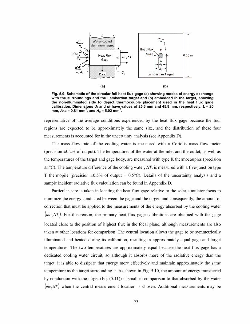
73

(a) (b)

Fig. 5.9: Schematic of the circular foil heat flux gage (a) showing modes of energy exchange with the surroundings and the Lambertian target and (b) embedded in the target, showing the non-illuminated side to depict thermocouple placement used in the heat flux gage calibration. Dimensions d1 and d2 have values of 25.3 mm and 45.8 mm, respectively, L = 20 mm, Afoil = 0.81 mm

2, and Ag = 5.02 mm

2.

representative of the average conditions experienced by the heat flux gage because the four

regions are expected to be approximately the same size, and the distribution of these four

measurements is accounted for in the uncertainty analysis (see Appendix D).

The mass flow rate of the cooling water is measured with a Coriolis mass flow meter

(precision ±0.2% of output). The temperatures of the water at the inlet and the outlet, as well as

the temperatures of the target and gage body, are measured with type K thermocouples (precision

±1°C). The temperature difference of the cooling water, T, is measured with a five-junction type

T thermopile (precision ±0.5% of output + 0.5°C). Details of the uncertainty analysis and a

sample incident radiative flux calculation can be found in Appendix D.

Particular care is taken in locating the heat flux gage relative to the solar simulator focus to

minimize the energy conducted between the gage and the target, and consequently, the amount of

correction that must be applied to the measurements of the energy absorbed by the cooling water

Tcm p . For this reason, the primary heat flux gage calibrations are obtained with the gage

located close to the position of highest flux in the focal plane, although measurements are also

taken at other locations for comparison. The central location allows the gage to be symmetrically

illuminated and heated during its calibration, resulting in approximately equal gage and target

temperatures. The two temperatures are approximately equal because the heat flux gage has a

dedicated cooling water circuit, so although it absorbs more of the radiative energy than the

target, it is able to dissipate that energy more effectively and maintain approximately the same

temperature as the target surrounding it. As shown in Fig. 5.10, the amount of energy transferred

by conduction with the target (Eq. (5.11)) is small in comparison to that absorbed by the water

Tcm p when the central measurement location is chosen. Additional measurements may be

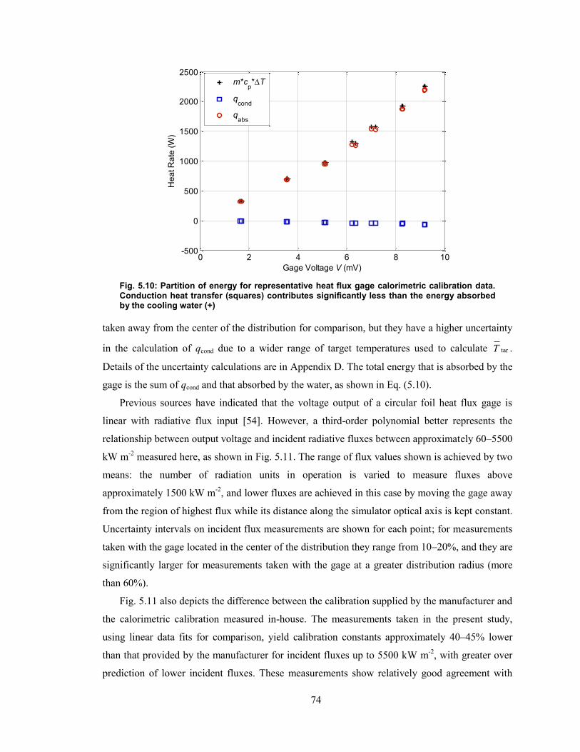
74

Fig. 5.10: Partition of energy for representative heat flux gage calorimetric calibration data. Conduction heat transfer (squares) contributes significantly less than the energy absorbed by the cooling water (+)

taken away from the center of the distribution for comparison, but they have a higher uncertainty

in the calculation of qcond due to a wider range of target temperatures used to calculate tarT .

Details of the uncertainty calculations are in Appendix D. The total energy that is absorbed by the

gage is the sum of qcond and that absorbed by the water, as shown in Eq. (5.10).

Previous sources have indicated that the voltage output of a circular foil heat flux gage is

linear with radiative flux input [54]. However, a third-order polynomial better represents the

relationship between output voltage and incident radiative fluxes between approximately 60–5500

kW m-2

measured here, as shown in Fig. 5.11. The range of flux values shown is achieved by two

means: the number of radiation units in operation is varied to measure fluxes above

approximately 1500 kW m-2

, and lower fluxes are achieved in this case by moving the gage away

from the region of highest flux while its distance along the simulator optical axis is kept constant.

Uncertainty intervals on incident flux measurements are shown for each point; for measurements

taken with the gage located in the center of the distribution they range from 10–20%, and they are

significantly larger for measurements taken with the gage at a greater distribution radius (more

than 60%).

Fig. 5.11 also depicts the difference between the calibration supplied by the manufacturer and

the calorimetric calibration measured in-house. The measurements taken in the present study,

using linear data fits for comparison, yield calibration constants approximately 40–45% lower

than that provided by the manufacturer for incident fluxes up to 5500 kW m-2

, with greater over

prediction of lower incident fluxes. These measurements show relatively good agreement with

0 2 4 6 8 10-500

0

500

1000

1500

2000

2500

Gage Voltage V (mV)

He

at R

ate

(W

)

m*cp*T

qcond

qabs

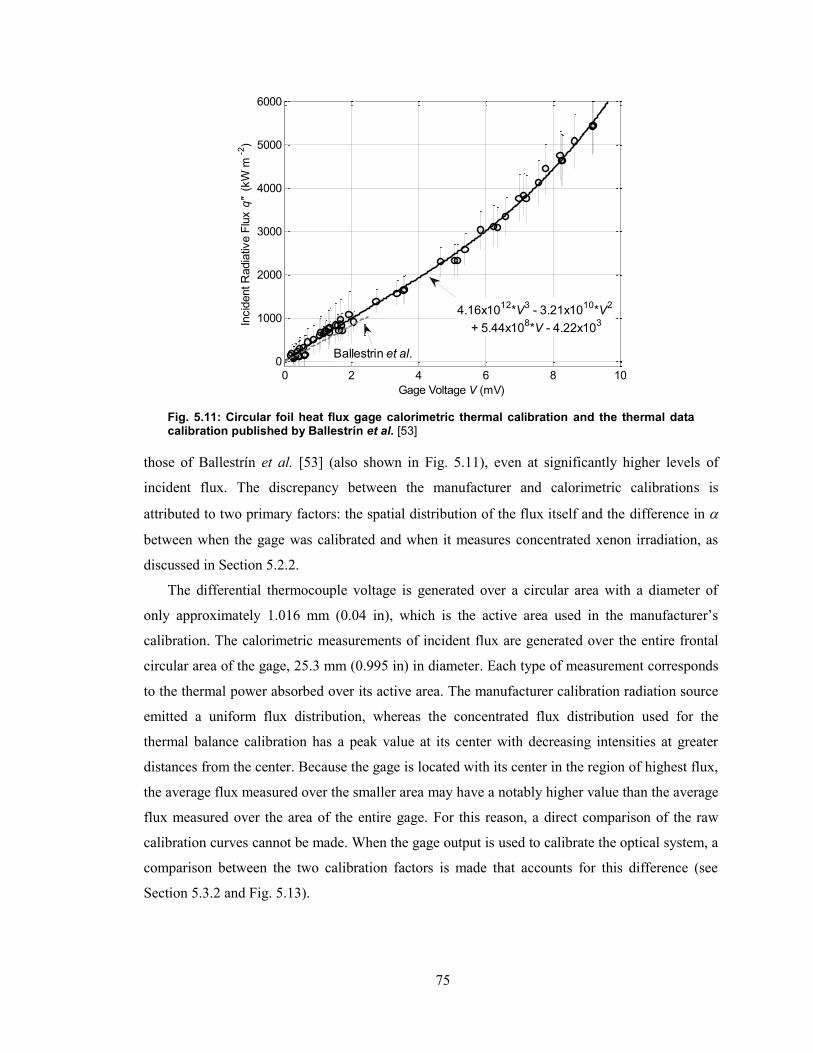
75

Fig. 5.11: Circular foil heat flux gage calorimetric thermal calibration and the thermal data calibration published by Ballestrín et al. [53]

those of Ballestrín et al. [53] (also shown in Fig. 5.11), even at significantly higher levels of

incident flux. The discrepancy between the manufacturer and calorimetric calibrations is

attributed to two primary factors: the spatial distribution of the flux itself and the difference in

between when the gage was calibrated and when it measures concentrated xenon irradiation, as

discussed in Section 5.2.2.

The differential thermocouple voltage is generated over a circular area with a diameter of

only approximately 1.016 mm (0.04 in), which is the active area used in the manufacturer’s

calibration. The calorimetric measurements of incident flux are generated over the entire frontal

circular area of the gage, 25.3 mm (0.995 in) in diameter. Each type of measurement corresponds

to the thermal power absorbed over its active area. The manufacturer calibration radiation source

emitted a uniform flux distribution, whereas the concentrated flux distribution used for the

thermal balance calibration has a peak value at its center with decreasing intensities at greater

distances from the center. Because the gage is located with its center in the region of highest flux,

the average flux measured over the smaller area may have a notably higher value than the average

flux measured over the area of the entire gage. For this reason, a direct comparison of the raw

calibration curves cannot be made. When the gage output is used to calibrate the optical system, a

comparison between the two calibration factors is made that accounts for this difference (see

Section 5.3.2 and Fig. 5.13).

0 2 4 6 8 10

0

1000

2000

3000

4000

5000

6000

Gage Voltage V (mV)

Incid

ent R

adia

tive F

lux q

" (

kW

m -

2)

4.16x1012

*V3 - 3.21x10

10*V

2

+ 5.44x108*V - 4.22x10

3

Ballestrin et al.

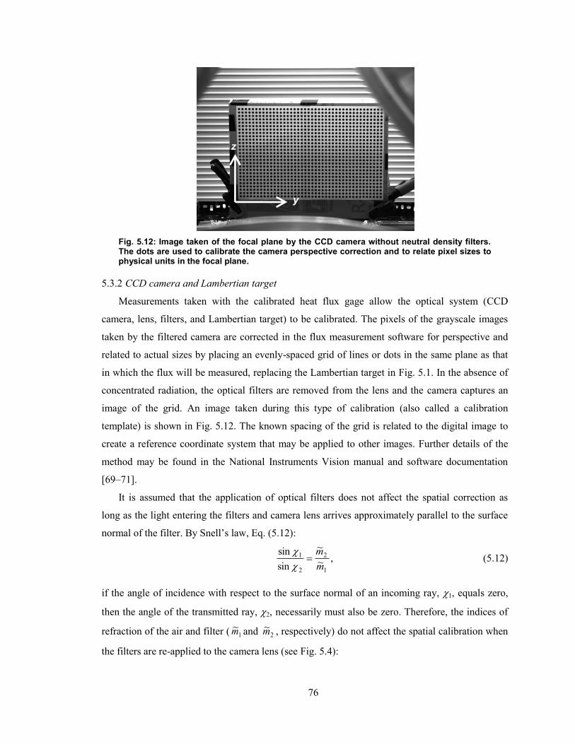
76

Fig. 5.12: Image taken of the focal plane by the CCD camera without neutral density filters. The dots are used to calibrate the camera perspective correction and to relate pixel sizes to physical units in the focal plane.

5.3.2 CCD camera and Lambertian target

Measurements taken with the calibrated heat flux gage allow the optical system (CCD

camera, lens, filters, and Lambertian target) to be calibrated. The pixels of the grayscale images

taken by the filtered camera are corrected in the flux measurement software for perspective and

related to actual sizes by placing an evenly-spaced grid of lines or dots in the same plane as that

in which the flux will be measured, replacing the Lambertian target in Fig. 5.1. In the absence of

concentrated radiation, the optical filters are removed from the lens and the camera captures an

image of the grid. An image taken during this type of calibration (also called a calibration

template) is shown in Fig. 5.12. The known spacing of the grid is related to the digital image to

create a reference coordinate system that may be applied to other images. Further details of the

method may be found in the National Instruments Vision manual and software documentation

[69–71].

It is assumed that the application of optical filters does not affect the spatial correction as

long as the light entering the filters and camera lens arrives approximately parallel to the surface

normal of the filter. By Snell’s law, Eq. (5.12):

,~

~

sin

sin

1

2

2

1

m

m

(5.12)

if the angle of incidence with respect to the surface normal of an incoming ray, 1, equals zero,

then the angle of the transmitted ray, 2, necessarily must also be zero. Therefore, the indices of

refraction of the air and filter ( 1~m and 2

~m , respectively) do not affect the spatial calibration when

the filters are re-applied to the camera lens (see Fig. 5.4):

y

z

77

After the spatial correction has been applied, the grayscale levels of the digital images are

related to measured values of radiant heat flux, incorporating inherent alterations of the flux

reflected by the target and intercepted by the CCD chip introduced by the target surface, the

neutral density filters, the lens, and the CCD chip itself due to the individual spectral

transmittances and sensitivities previously discussed. In order to relate the grayscale values

recorded by the CCD camera to radiative flux incident at the measurement plane, the incident flux

is first measured with the circular foil heat flux gage, both calorimetrically and using the

manufacturer calibration for comparison. The calorimetrically-measured incident flux is averaged

over the entire gage face (25.3 mm), whereas the flux measured using the manufacturer

calibration is averaged over the foil area (1.016 mm). Then, the heat flux gage is removed from

its measurement position and replaced by the cooled Lambertian surface. The optical system is

used to record an image. The grayscale values gs in the region of the image that was previously

occupied by the heat flux gage (25.3 mm or 1.016 mm with the same location) are analyzed

in order to determine the optical calibration constant Kf, calculated by:

gs

tyxqK

exp

f

. (5.13)

where texp is the camera exposure time and each pixel captures a square in the focal plane x = y

= 0.6907±0.0028 mm on a side. Conceptually, the measured rate of energy absorbed by the gage

qabs is related to the local incident flux by integrating over the area of the gage face Ag:

,dg

abs A

Aqq (5.14)

and the optical system is similarly used to determine the absorbed heat rate in the same region by:

gg

ddexp

f

exp

fabs

AAAgs

tyx

KA

tyx

gsKq

. (5.15)

For this reason, integrated and averaged values of both flux and grayscale may also be equated

and used to compute f.

The averaged grayscale values are plotted against the incident flux measured by the heat flux

gage, as shown in Fig. 5.13. Different flux levels were achieved for the optical calibration by

varying the number of radiation units in operation (the gage remains stationary).

When the manufacturer’s calibration is used for the optical calibration, the slope of the

calibration curve is 32% higher than the slope of the curve using the calorimetric heat flux gage

calibration. This difference is largely accounted for by the spectral considerations discussed in

78

Fig. 5.13: Incident radiative flux as a function of the grayscale levels averaged over an area corresponding to that of the appropriate active area. Squares and gray lines represent the measurements taken using the manufacturer calibration, whereas circles and black lines represent the values measured using the thermal balance method. The solid lines show the linear fit and the dashed lines show standard error intervals on the linear fit.

Fig. 5.14: Schematic showing the error encountered by approximating a circular area (dashed) by two square pixels (solid)

Section 5.2.2. Although only a 7% difference is accounted for by these spectral absorptivity

considerations (see Table 5.1), only the published xenon emission spectrum data (250–1650 nm)

can be used. Additional energy emitted and absorbed at longer wavelengths may further alter the

real value of , but cannot be accounted for with the provided data. An increased total

hemispherical absorptivity of the heat flux gage results in increased qabs or output voltage,

depending on the measurement method, over what would register if the same level of irradiation

was provided by a blackbody at 1123 K.

The larger standard error of the linear fit (±20%, shown with gray dashed lines) using the

manufacturer calibration is primarily due to the uncertainty in matching the foil area with the

pixel grayscales, whereas the standard error of the linear fit using the calorimetric calibration

(±12%, shown in black dashed lines) is due to the uncertainty in the determination of the incident

heat flux, particularly in determining qcond (see Appendix E for further detail). The match between

0 500 1000 1500 2000 2500 3000 35000

1000

2000

3000

4000

5000

6000

7000

8000

9000

10000

gs

Incid

en

t R

ad

iative

Flu

x q

" (k

W m

-2)

Thermal balancecalibration

Manufacturercalibration

79

the fluxes measured with the manufacturer’s calibration and the appropriate grayscales presents

two challenges: determining the pixels in the same location of the foil and the difference in areas

occupied by the actual foil area and the pixels analyzed. Although the small area of the circular

foil corresponds to a finer spatial resolution in flux measurements, any inaccuracy in selecting the

two pixels that align with the 1.016 mm (0.04 in) diameter foil bears a higher consequence than

inaccuracies introduced by misaligning the 1020 pixels used to approximate the 25.3 mm (0.995

in) diameter gage face. The larger area occupied by the gage allows for more pixel grayscale

values to be averaged and decreases the dependence on selecting the correct pixels. Additionally,

the area occupied by the two square pixels approximating the circular foil is 18% larger than the

area occupied by the foil, intercepting extra energy that is not actually absorbed by the gage. This

effect is shown schematically in Fig. 5.14.

The measured calibration data presented in Fig. 5.13 using the thermal gage calibration

(circles) are linear with a slope m of 1920±233 W m-2

with a zero intercept. The images were

taken with texp=60 ms. These data yield a calibration constant Kf of (5.5±0.7)×10-5

W s that

assumes a linear relation in the camera between the grayscale output and the energy input.

Because the integral and average flux and grayscale values may be use in the optical flux

calibration, the specific value is calculated by Eq. (5.16):

exp

exp

f tyxmgs

tyxqK

. (5.16)

The values of uncertainty in m and Kf incorporate contributions from the incident flux

measurements (including temperatures, mass flow rate, and change in temperature for the

calorimetric method), the digital least count of the camera (a step of one grayscale value), the

resolution of the printer used to print the grid of dots for the spatial calibration, the slightly

different areas occupied by the studied grayscales and the heat flux gage, and the standard error

of the linear fit (see Figliola & Beasley [72]). Details of the optical uncertainty calculation can be

found in Appendix E.

Some important factors must be considered in determining the location within the

measurement plane used to calibrate the camera grayscale output. Because the grayscale value

used in Eq. (5.16) is averaged over a relatively large area the size of the circular foil heat flux

gage (25.3 mm), an ideal calibration region would exhibit low gradients of radiative flux to

ensure that the average fluxes and grayscales are truly representative values; however, regions of

this nature in the focal plane of the solar simulator are nonexistent for flux levels that are

important in the overall radiative output. While a substitute radiation source that produces a

80

spatially flat flux distribution could be used solely for the flux-to-grayscale calibration, the

substitute source must have exactly the same spectral distribution as the solar simulator. The

reason for this is that this optical method of heat flux measurement relies on relating the radiative

flux registered by the CCD chip, which, along with the lens and filters, has its own spectral

sensitivity, to the radiative flux incident on the target, as previously discussed. Any spectral

deviations between the calibration and measurement sources therefore would introduce

systematic errors into the measurements. Due to the challenge of finding a suitable substitute

radiation source, the flux calibration is carried out in the focus of the solar simulator. These

calibration techniques were completed with the use of a previously developed data acquisition

platform [71], which provides the foundation for further data acquisition programs developed for

this project as needed. Software documentation contains more detailed information on this data

acquisition platform and specific calibration instructions [71].

Furthermore, the optical calibration technique for obtaining flux measurements requires that

all optical components (the target surface, camera, filters, lens) and the output spectral

distribution of the simulator remain unchanged between calibration and measurements. The effect

of the filters, lens, and camera has been discussed in Section 5.2.2, but the target surface also

plays an important role in the optical measurements. If the reflectivity of the target decreased

uniformly by 5% (for example, by becoming soiled), 5% less radiation would reach the filters,

lens, and camera, and a corresponding decrease of 5% in the grayscale output of the CCD camera

would result for the same amount of radiative flux incident at the measurement plane. It should be

noted that a slight difference (approximately 2–6%) has been noted between measurements taken

with the plain (continuous) target and with the target equipped with a hole to house the heat flux

gage (see Appendix F for data). For this reason, both the optical calibration and the optical

measurements are completed using photographs taken of radiation reflected from the plain target.

As similarly discussed in Section 5.2.2, the simulator output spectral distribution is assumed

to be identical at all locations in the measurement plane and consistent between calibration and

measurement. If the spectral output of the xenon arc lamps changes over their lifetime, which

may occur due to degradation of the electrodes, the optical measurement system may require

recalibration. However, the expected magnitude and nature of such spectral changes would likely

be similar to the spatially-varying spectral distributions discussed in Section 5.2.2, and would

likely cause minimal disturbance to the measurement system. Flux measurements should be

periodically recorded and compared to previous measurements. If a significant change in flux is

noted (e.g., more than 10% difference), then the optical measurement system should be

recalibrated.

81

Chapter 6

Measured Solar Simulator Performance

Flux maps are taken of the outputs of individual radiation units, in addition to the total

simulator output. The combination of seven lamps can provide up to 9.2±1.1 kW over a 60-mm

diameter circular area located in the focal plane, corresponding to an average flux of 3240±390

kW m-2

, with a peak flux of 7300±890 kW m-2

. The individual flux maps are superposed and

compared to the flux map taken with multiple lamps operating concurrently, which confirms the

assumption used in Chapter 3 that individual outputs may be superposed without loss of accuracy.

Additionally, the output of the solar simulator is measured as a function of time, which shows that

the output is steady to within the measurement uncertainty after an initial warm up period of

approximately 15 minutes. Finally, measured flux maps are compared to those generated with

Monte Carlo ray tracing as described in Chapter 3, and differences between them are discussed in

terms of assumptions used in the model.

6.1 Measurement Methods

6.1.1 Spatial flux

Spatial flux distributions were measured using the calibrated CCD camera and target after the

lamps had warmed up for at least fifteen minutes to reach a steady output. Measured flux

distributions were obtained by applying the appropriate calibrations described in Section 5.3 to an

average image generated by at least thirty grayscale images taken once per second in order to

minimize the effects of noise in the output of the lamps. In the results presented here, the optical

calibration obtained using the thermal balance heat flux gage calibration is used in order to

account for the effects of the spectral absorptivity of the gage coating, as described in Section

5.2.2, and to minimize the calibration uncertainty, as shown in Fig. 5.13.

Metrics used to evaluate the solar simulator performance include the blackbody stagnation

temperature, Tb, the flux non-uniformity f, and the delivery efficiency . The blackbody

stagnation temperature is the maximum theoretical temperature that a blackbody receiver would

reach for a given flux input with no losses, as calculated by Eq. (1.1). The flux non-uniformity

describes the distribution of the radiative flux in the focal plane. The definition used in Chapter 3,

Eq. (3.34), is applied here with the following simplification:

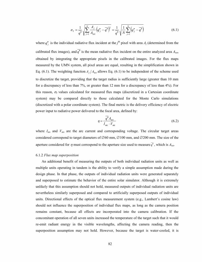
82

N

j

j

N

j

j

jqq

Nqqq

A

A

qσ

11

2

tot

f

111 (6.1)

wherejq is the individual radiative flux incident at the j

th pixel with area Aj (determined from the

calibrated flux images), and q is the mean radiative flux incident on the entire analyzed area Atot,

obtained by integrating the appropriate pixels in the calibrated images. For the flux maps

measured by the UMN system, all pixel areas are equal, resulting in the simplification shown in

Eq. (6.1). The weighting function totAA j allows Eq. (6.1) to be independent of the scheme used

to discretize the target, providing that the target radius is sufficiently large (greater than 10 mm

for a discrepancy of less than 7%, or greater than 12 mm for a discrepancy of less than 4%). For

this reason, f values calculated for measured flux maps (discretized in a Cartesian coordinate

system) may be compared directly to those calculated for the Monte Carlo simulations

(discretized with a polar coordinate system). The final metric is the delivery efficiency of electric

power input to radiative power delivered to the focal area, defined by:

arcarc

tot

VI

Aqη

(6.2)

where Iarc and Varc are the arc current and corresponding voltage. The circular target areas

considered correspond to target diameters of 60 mm, 100 mm, and 200 mm. The size of the

aperture considered for must correspond to the aperture size used to measure q , which is Atot.

6.1.2 Flux map superposition

An additional benefit of measuring the outputs of both individual radiation units as well as

multiple units operating in tandem is the ability to verify a simple assumption made during the

design phase. In that phase, the outputs of individual radiation units were generated separately

and superposed to estimate the behavior of the entire solar simulator. Although it is extremely

unlikely that this assumption should not hold, measured outputs of individual radiation units are

nevertheless similarly superposed and compared to artificially superposed outputs of individual

units. Directional effects of the optical flux measurement system (e.g., Lambert’s cosine law)

should not influence the superposition of individual flux maps, as long as the camera position

remains constant, because all effects are incorporated into the camera calibration. If the

concomitant operation of all seven units increased the temperature of the target such that it would

re-emit radiant energy in the visible wavelengths, affecting the camera reading, then the

superposition assumption may not hold. However, because the target is water-cooled, it is

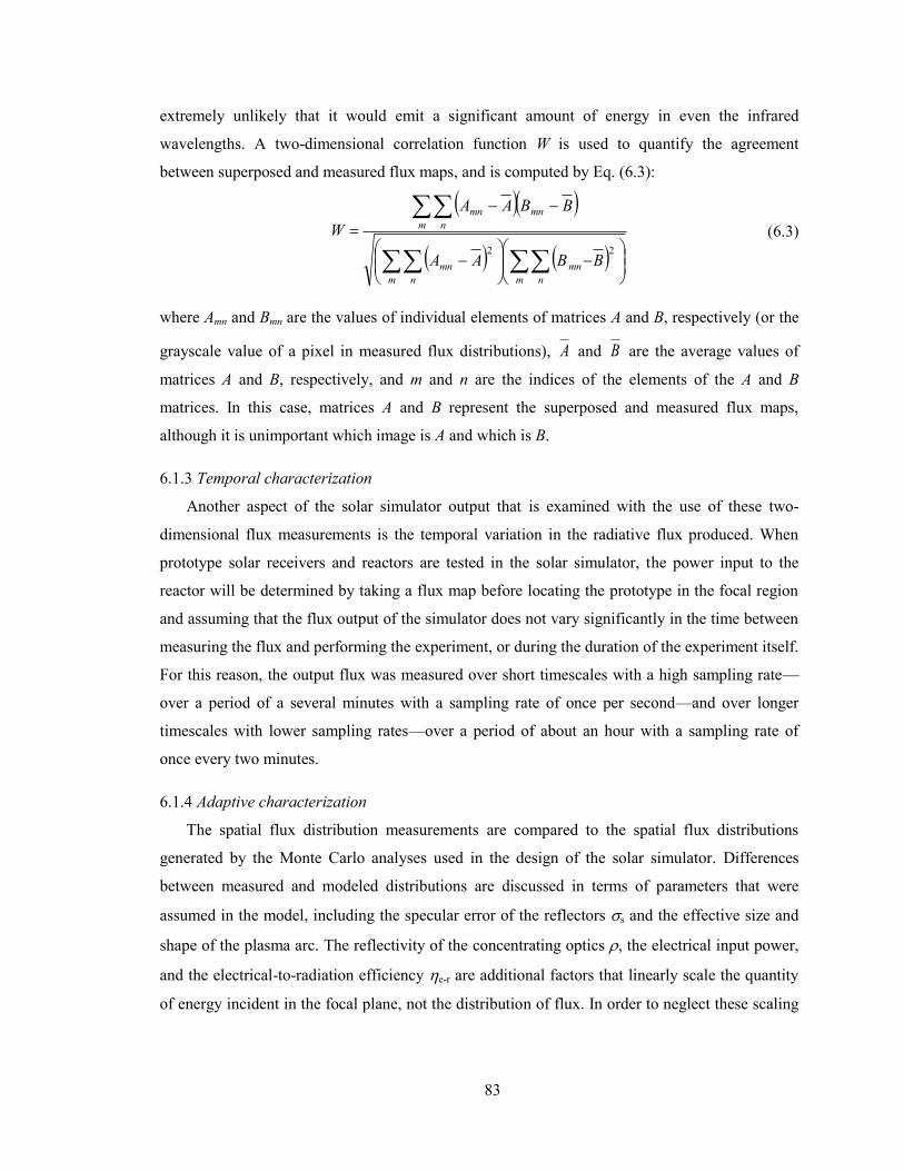
83

extremely unlikely that it would emit a significant amount of energy in even the infrared

wavelengths. A two-dimensional correlation function W is used to quantify the agreement

between superposed and measured flux maps, and is computed by Eq. (6.3):

m n

mn

m n

mn

m n

mnmn

BBAA

BBAA

W22

(6.3)

where Amn and Bmn are the values of individual elements of matrices A and B, respectively (or the

grayscale value of a pixel in measured flux distributions), A and B are the average values of

matrices A and B, respectively, and m and n are the indices of the elements of the A and B

matrices. In this case, matrices A and B represent the superposed and measured flux maps,

although it is unimportant which image is A and which is B.

6.1.3 Temporal characterization

Another aspect of the solar simulator output that is examined with the use of these two-

dimensional flux measurements is the temporal variation in the radiative flux produced. When

prototype solar receivers and reactors are tested in the solar simulator, the power input to the

reactor will be determined by taking a flux map before locating the prototype in the focal region

and assuming that the flux output of the simulator does not vary significantly in the time between

measuring the flux and performing the experiment, or during the duration of the experiment itself.

For this reason, the output flux was measured over short timescales with a high sampling rate—

over a period of a several minutes with a sampling rate of once per second—and over longer

timescales with lower sampling rates—over a period of about an hour with a sampling rate of

once every two minutes.

6.1.4 Adaptive characterization

The spatial flux distribution measurements are compared to the spatial flux distributions

generated by the Monte Carlo analyses used in the design of the solar simulator. Differences

between measured and modeled distributions are discussed in terms of parameters that were

assumed in the model, including the specular error of the reflectors s and the effective size and

shape of the plasma arc. The reflectivity of the concentrating optics , the electrical input power,

and the electrical-to-radiation efficiency e-r are additional factors that linearly scale the quantity

of energy incident in the focal plane, not the distribution of flux. In order to neglect these scaling

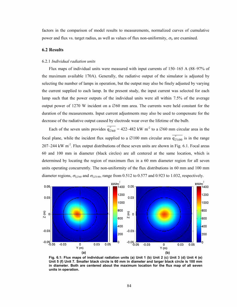
84

factors in the comparison of model results to measurements, normalized curves of cumulative

power and flux vs. target radius, as well as values of flux non-uniformity, f, are examined.

6.2 Results

6.2.1 Individual radiation units

Flux maps of individual units were measured with input currents of 150–165 A (88–97% of

the maximum available 170A). Generally, the radiative output of the simulator is adjusted by

selecting the number of lamps in operation, but the output may also be finely adjusted by varying

the current supplied to each lamp. In the present study, the input current was selected for each

lamp such that the power outputs of the individual units were all within 7.5% of the average

output power of 1270 W incident on a 60 mm area. The currents were held constant for the

duration of the measurements. Input current adjustments may also be used to compensate for the

decrease of the radiative output caused by electrode wear over the lifetime of the bulb.

Each of the seven units provides = 422–482 kW m

-2 to a 60 mm circular area in the

focal plane, while the incident flux supplied to a 100 mm circular area is in the range

207–244 kW m-2

. Flux output distributions of these seven units are shown in Fig. 6.1. Focal areas

60 and 100 mm in diameter (black circles) are all centered at the same location, which is

determined by locating the region of maximum flux in a 60 mm diameter region for all seven

units operating concurrently. The non-uniformity of the flux distributions in 60 mm and 100 mm

diameter regions, f,60 and f,, range from 0.512 to 0.577 and 0.923 to 1.032, respectively.

(a)

(b)

Fig. 6.1: Flux maps of individual radiation units (a) Unit 1 (b) Unit 2 (c) Unit 3 (d) Unit 4 (e) Unit 5 (f) Unit 7. Smaller black circle is 60 mm in diameter and larger black circle is 100 mm in diameter. Both are centered about the maximum location for the flux map of all seven units in operation.

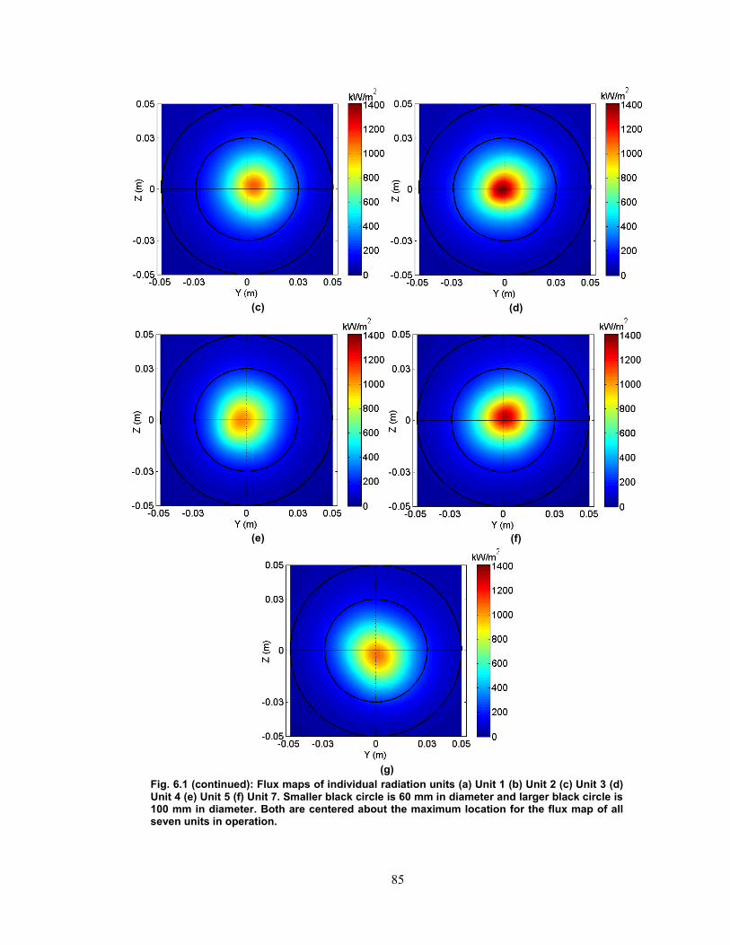
85

(c)

(d)

(e)

(f)

(g)

Fig. 6.1 (continued): Flux maps of individual radiation units (a) Unit 1 (b) Unit 2 (c) Unit 3 (d) Unit 4 (e) Unit 5 (f) Unit 7. Smaller black circle is 60 mm in diameter and larger black circle is 100 mm in diameter. Both are centered about the maximum location for the flux map of all seven units in operation.

86

Table 6.1: Summary of individual radiation unit outputs

Unit I (A) Varc (V)

(kW m-2

) 60 f,60

(kW m-2

) 100 f100 200

1 165 34.3 422 0.211 0.558 220 0.306 0.954 0.473

2 150 33.0 467 0.267 0.517 230 0.366 1.006 0.515

3 155 34.0 426 0.229 0.525 223 0.333 0.923 0.490

4 150 34.3 482 0.266 0.569 244 0.373 1.004 0.531

5 150 33.5 419 0.236 0.549 207 0.325 1.021 0.477

6 150 33.3 472 0.268 0.577 236 0.372 1.032 0.522

7 150 33.0 451 0.258 0.512 229 0.364 0.956 0.518

All

3240 0.255 0.496 1670 0.366 0.917 0.557

(a)

(b)

(c)

(d)

Fig. 6.2: Plots of one-dimensional flux taken along the y- and z-directions of the two-dimensional flux maps for individual units: (a) Unit 1 (b) Unit 2 (c) Unit 3 (d) Unit 4 (e) Unit 5 (f) Unit 7. Distributions that are not exactly centered at the origin have a redefined zero in order to examine the symmetry, rather than location, of the distribution.

-100 -50 0 50 1000

200

400

600

800

1,000

1,200

1,400

Location, y or z (mm)

Ce

nte

red

in

cid

en

t flu

x, q"

(kW

m-2

)

Lamp 1

y

z

-100 -50 0 50 1000

200

400

600

800

1,000

1,200

1,400


Cente

red incid

ent flux, q"

(kW

m-2

)

Lamp 2

y

z

-100 -50 0 50 1000

200

400

600

800

1,000

1,200

1,400


Ce

nte

red

in

cid

en

t flu

x, q"

(kW

m-2

)

Lamp 3

y

z

-100 -50 0 50 1000

200

400

600

800

1,000

1,200

1,400


Cente

red incid

ent flux, q"

(kW

m-2

)

Lamp 4

y

z

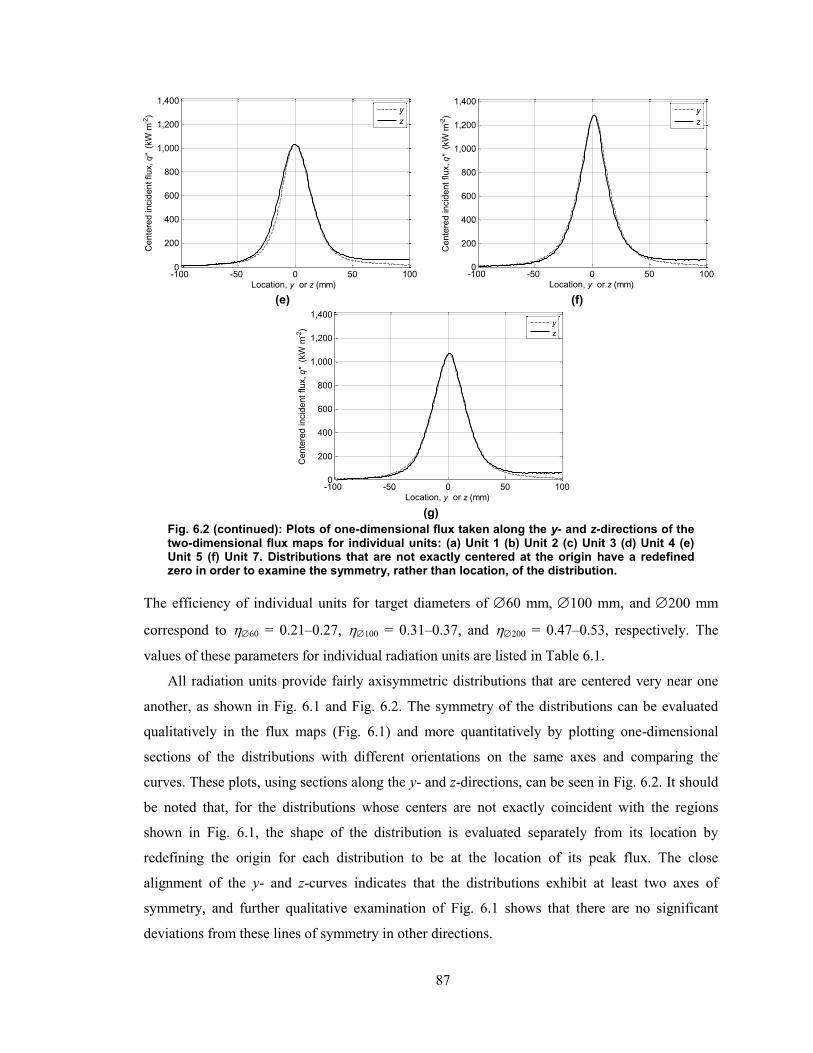
87

(e)

(f)

(g)

Fig. 6.2 (continued): Plots of one-dimensional flux taken along the y- and z-directions of the two-dimensional flux maps for individual units: (a) Unit 1 (b) Unit 2 (c) Unit 3 (d) Unit 4 (e) Unit 5 (f) Unit 7. Distributions that are not exactly centered at the origin have a redefined zero in order to examine the symmetry, rather than location, of the distribution.

The efficiency of individual units for target diameters of 60 mm, 100 mm, and 200 mm

correspond to 60 = 0.21–0.27, 100 = 0.31–0.37, and 200 = 0.47–0.53, respectively. The

values of these parameters for individual radiation units are listed in Table 6.1.

All radiation units provide fairly axisymmetric distributions that are centered very near one

another, as shown in Fig. 6.1 and Fig. 6.2. The symmetry of the distributions can be evaluated

qualitatively in the flux maps (Fig. 6.1) and more quantitatively by plotting one-dimensional

sections of the distributions with different orientations on the same axes and comparing the

curves. These plots, using sections along the y- and z-directions, can be seen in Fig. 6.2. It should

be noted that, for the distributions whose centers are not exactly coincident with the regions

shown in Fig. 6.1, the shape of the distribution is evaluated separately from its location by

redefining the origin for each distribution to be at the location of its peak flux. The close

alignment of the y- and z-curves indicates that the distributions exhibit at least two axes of

symmetry, and further qualitative examination of Fig. 6.1 shows that there are no significant

deviations from these lines of symmetry in other directions.

-100 -50 0 50 1000

200

400

600

800

1,000

1,200

1,400


Ce

nte

red

in

cid

en

t flu

x, q"

(kW

m-2

)

Lamp 5

y

z

-100 -50 0 50 1000

200

400

600

800

1,000

1,200

1,400


Ce

nte

red

in

cid

en

t flu

x, q"

(kW

m-2

)

Lamp 6

y

z

-100 -50 0 50 1000

200

400

600

800

1,000

1,200

1,400


Cente

red incid

ent flux, q"

(kW

m-2

)Lamp 7

y

z

88

The design conditions presented in Chapter 2 and Chapter 3 are met by focusing the solar

simulator by adjusting the position of each lamp with respect to the reflector (as described in

Appendix B). The optimal lamp position for the focusing procedure is determined by maximizing

the amount of radiative power provided to a 60 mm circular area in the focal plane, q60. The

location of this circular focal area is determined based on the location of the spot generated by the

central radiation unit, #4. Ideally, the focused position is such that the brightest portion of the arc

is coincident with the focus of the ellipsoidal reflector. Although this condition is achieved at the

expense of increasing the flux non-uniformity, which could possibly lead to uneven heating of

receiver/reactor prototypes, it is selected to avoid significant loss of radiative power provided by

the solar simulator (up to 42%), which would result from the separation of the lamp arc from the

ellipsoid focus. As an example, the flux maps of unit #4 measured before and after its focus was

adjusted are shown in Fig. 6.3. Before the focusing procedure, 343 kW m-2

of thermal energy was

provided to a 60mm focal area with a flux uniformity of f = 0.415. After its focus was

adjusted, its flux output increased to 488 kW m-2

to a 60mm focal area and the flux non-

uniformity increased to f = 0.561. The 42% decrease in delivered radiative flux that would occur

from defocusing the solar simulator is not considered worth the 35% decrease in flux non-

uniformity.

6.2.2 Complete solar simulator performance

A flux map taken with all seven radiation units operating concurrently with the input currents

listed in Table 6.1, is shown in Fig. 6.4. Under these conditions, the solar simulator is capable of

(a) (b)

Fig. 6.3: Comparitive flux maps of radiation unit #4 (a) before and (b) after the lamp position was adjusted and optimized with respect to the reflector

89

providing q60 = 9.2±1.1 kW of thermal power to a focal area 60 mm in diameter, corresponding

to an average flux of = 3240±390 kW m

-2 with a non-uniformity of f,60 = 0.50. Over a

100 mm diameter focal area, the mean flux is 1670±200 kW m-2

, and the peak flux is 7300±890

kW m-2

, as averaged over a focal area 10 mm in diameter. This flux map indicates that the

distribution is highly axisymmetric and provides concentrations sufficient to achieve a blackbody

stagnation temperature Tb of over 2740 K (60 mm—see Eq. (1.1)), sufficiently meeting the

goals set forth in the design stage (see Chapter 1 and Chapter 2). As with the individual radiation

unit flux maps, a symmetry plot showing two one-dimensional flux curves in the y- and z-

directions for the entire solar simulator are shown in Fig. 6.5.

Cumulative average flux and power vs. target radius curves are shown in Fig. 6.6. The

general shapes of the curves agree with expected behavior of a concentrating system as depicted

in Chapter 1, as well as the curves generated using the design-phase Monte Carlo models,

meaning that the cumulative average incident flux reaches its maximum near a target radius of

zero, nearest the ideal focal point where most of the xenon arc is mapped. Similarly, the

cumulative power increases with the target radius due to the larger area available to intercept

radiation. Although flux and power data are provided for a target radius as large as 100 mm

(200 mm), it is not anticipated that reactors with apertures larger than a radius of 50 mm (100

mm) will be used.

Fig. 6.4: Spatial distribution of the output of all seven radiation units in the focal plane. The inner black circle is 60 mm in diameter, while the outer circle is 100 mm in diameter.

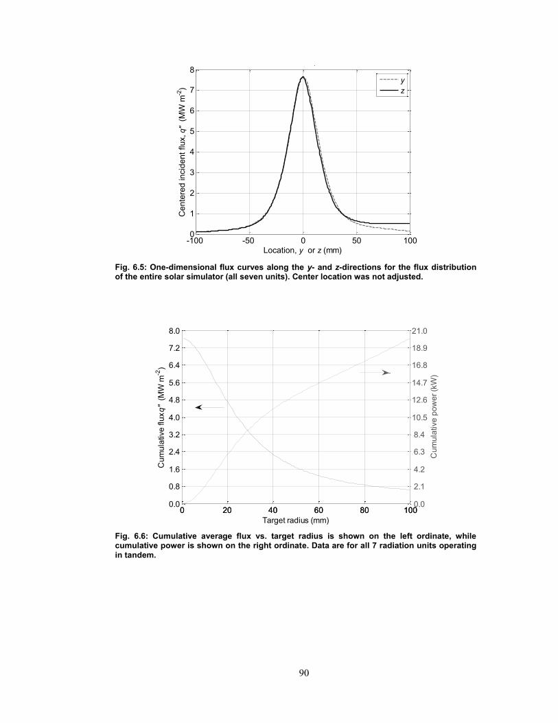
90

Fig. 6.5: One-dimensional flux curves along the y- and z-directions for the flux distribution of the entire solar simulator (all seven units). Center location was not adjusted.

Fig. 6.6: Cumulative average flux vs. target radius is shown on the left ordinate, while cumulative power is shown on the right ordinate. Data are for all 7 radiation units operating in tandem.

-100 -50 0 50 1000

1

2

3

4

5

6

7

8


Cente

red incid

ent flux, q"

(M

W m

-2)

All 7 lamps

y

z

0 20 40 60 80 1000.0

0.8

1.6

2.4

3.2

4.0

4.8

5.6

6.4

7.2

8.0

Cu

mu

lative

flu

x q

" (

MW

m-2

)

0 20 40 60 80 100 0.0

2.1

4.2

6.3

8.4

10.5

12.6

14.7

16.8

18.9

21.0

Cu

mu

lative

po

we

r (k

W)

Target radius (mm)

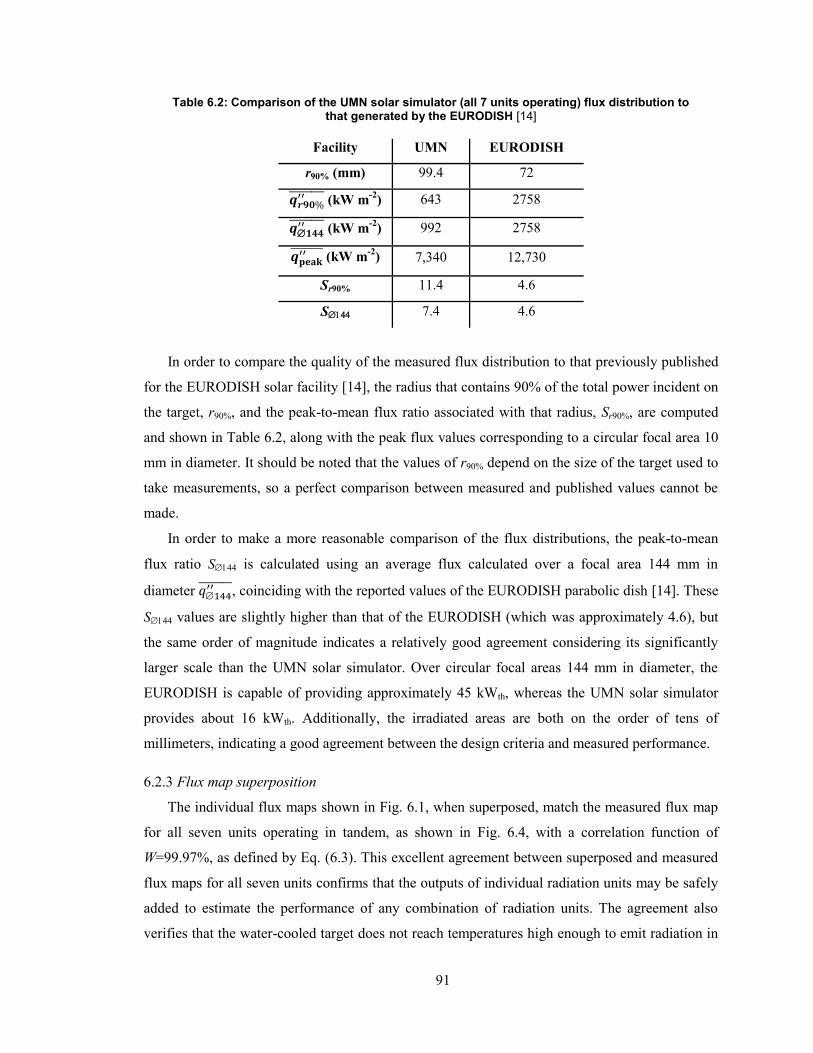
91

Table 6.2: Comparison of the UMN solar simulator (all 7 units operating) flux distribution to that generated by the EURODISH [14]

Facility UMN EURODISH

r90% (mm) 99.4 72

(kW m

-2) 643 2758

(kW m

-2) 992 2758

(kW m

-2) 7,340 12,730

Sr90% 11.4 4.6

S 7.4 4.6

In order to compare the quality of the measured flux distribution to that previously published

for the EURODISH solar facility [14], the radius that contains 90% of the total power incident on

the target, r90%, and the peak-to-mean flux ratio associated with that radius, Sr90%, are computed

and shown in Table 6.2, along with the peak flux values corresponding to a circular focal area 10

mm in diameter. It should be noted that the values of r90% depend on the size of the target used to

take measurements, so a perfect comparison between measured and published values cannot be

made.

In order to make a more reasonable comparison of the flux distributions, the peak-to-mean

flux ratio S is calculated using an average flux calculated over a focal area 144 mm in

diameter , coinciding with the reported values of the EURODISH parabolic dish [14]. These

S values are slightly higher than that of the EURODISH (which was approximately 4.6), but

the same order of magnitude indicates a relatively good agreement considering its significantly

larger scale than the UMN solar simulator. Over circular focal areas 144 mm in diameter, the

EURODISH is capable of providing approximately 45 kWth, whereas the UMN solar simulator

provides about 16 kWth. Additionally, the irradiated areas are both on the order of tens of

millimeters, indicating a good agreement between the design criteria and measured performance.

6.2.3 Flux map superposition

The individual flux maps shown in Fig. 6.1, when superposed, match the measured flux map

for all seven units operating in tandem, as shown in Fig. 6.4, with a correlation function of

W=99.97%, as defined by Eq. (6.3). This excellent agreement between superposed and measured

flux maps for all seven units confirms that the outputs of individual radiation units may be safely

added to estimate the performance of any combination of radiation units. The agreement also

verifies that the water-cooled target does not reach temperatures high enough to emit radiation in

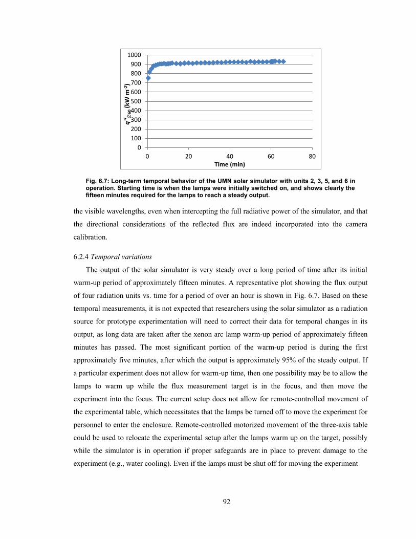
92

Fig. 6.7: Long-term temporal behavior of the UMN solar simulator with units 2, 3, 5, and 6 in operation. Starting time is when the lamps were initially switched on, and shows clearly the fifteen minutes required for the lamps to reach a steady output.

the visible wavelengths, even when intercepting the full radiative power of the simulator, and that

the directional considerations of the reflected flux are indeed incorporated into the camera

calibration.

6.2.4 Temporal variations

The output of the solar simulator is very steady over a long period of time after its initial

warm-up period of approximately fifteen minutes. A representative plot showing the flux output

of four radiation units vs. time for a period of over an hour is shown in Fig. 6.7. Based on these

temporal measurements, it is not expected that researchers using the solar simulator as a radiation

source for prototype experimentation will need to correct their data for temporal changes in its

output, as long data are taken after the xenon arc lamp warm-up period of approximately fifteen

minutes has passed. The most significant portion of the warm-up period is during the first

approximately five minutes, after which the output is approximately 95% of the steady output. If

a particular experiment does not allow for warm-up time, then one possibility may be to allow the

lamps to warm up while the flux measurement target is in the focus, and then move the

experiment into the focus. The current setup does not allow for remote-controlled movement of

the experimental table, which necessitates that the lamps be turned off to move the experiment for

personnel to enter the enclosure. Remote-controlled motorized movement of the three-axis table

could be used to relocate the experimental setup after the lamps warm up on the target, possibly

while the simulator is in operation if proper safeguards are in place to prevent damage to the

experiment (e.g., water cooling). Even if the lamps must be shut off for moving the experiment

0

100

200

300

400

500

600

700

800

900

1000

0 20 40 60 80

q''

60

(kW

m-2

)

Time (min)

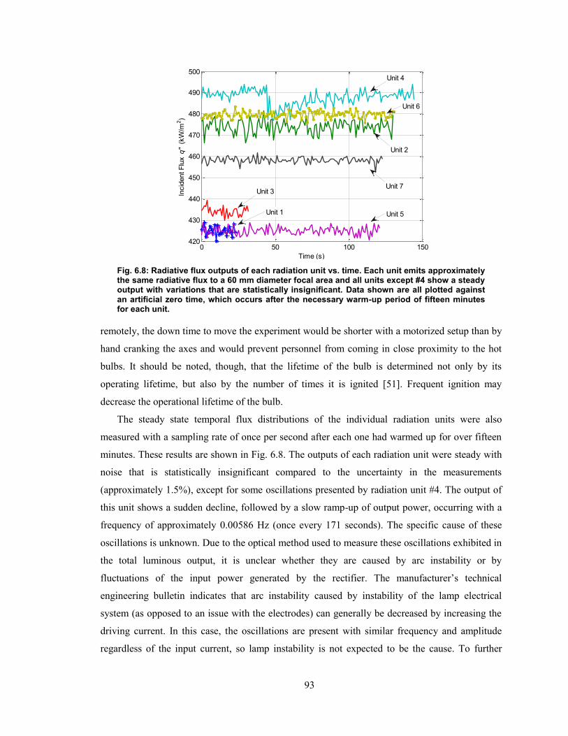
93

Fig. 6.8: Radiative flux outputs of each radiation unit vs. time. Each unit emits approximately the same radiative flux to a 60 mm diameter focal area and all units except #4 show a steady output with variations that are statistically insignificant. Data shown are all plotted against an artificial zero time, which occurs after the necessary warm-up period of fifteen minutes for each unit.

remotely, the down time to move the experiment would be shorter with a motorized setup than by

hand cranking the axes and would prevent personnel from coming in close proximity to the hot

bulbs. It should be noted, though, that the lifetime of the bulb is determined not only by its

operating lifetime, but also by the number of times it is ignited [51]. Frequent ignition may

decrease the operational lifetime of the bulb.

The steady state temporal flux distributions of the individual radiation units were also

measured with a sampling rate of once per second after each one had warmed up for over fifteen

minutes. These results are shown in Fig. 6.8. The outputs of each radiation unit were steady with

noise that is statistically insignificant compared to the uncertainty in the measurements

(approximately 1.5%), except for some oscillations presented by radiation unit #4. The output of

this unit shows a sudden decline, followed by a slow ramp-up of output power, occurring with a

frequency of approximately 0.00586 Hz (once every 171 seconds). The specific cause of these

oscillations is unknown. Due to the optical method used to measure these oscillations exhibited in

the total luminous output, it is unclear whether they are caused by arc instability or by

fluctuations of the input power generated by the rectifier. The manufacturer’s technical

engineering bulletin indicates that arc instability caused by instability of the lamp electrical

system (as opposed to an issue with the electrodes) can generally be decreased by increasing the

driving current. In this case, the oscillations are present with similar frequency and amplitude

regardless of the input current, so lamp instability is not expected to be the cause. To further

0 50 100 150420

430

440

450

460

470

480

490

500

Time (s)

Incid

ent F

lux q

" (

kW

/m2)

Unit 2

Unit 4

Unit 6

Unit 7Unit 3

Unit 5Unit 1

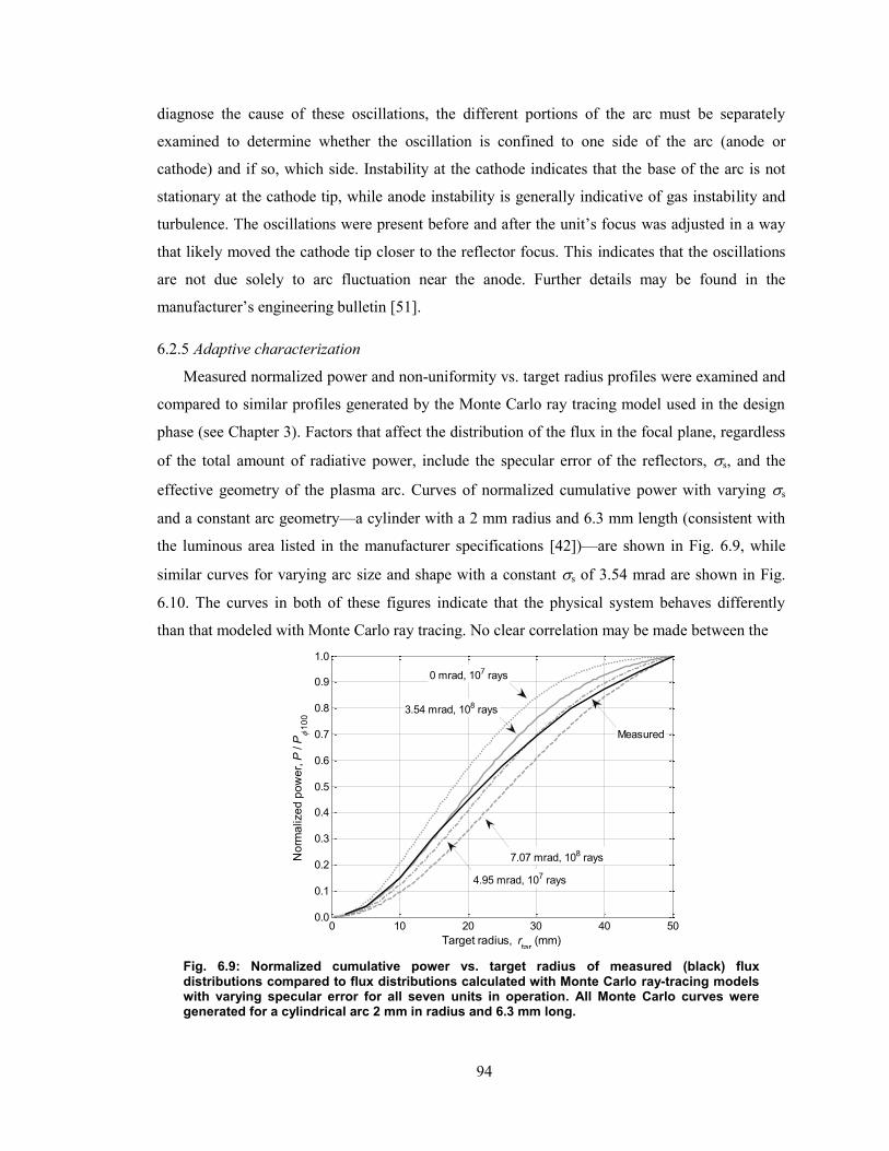
94

diagnose the cause of these oscillations, the different portions of the arc must be separately

examined to determine whether the oscillation is confined to one side of the arc (anode or

cathode) and if so, which side. Instability at the cathode indicates that the base of the arc is not

stationary at the cathode tip, while anode instability is generally indicative of gas instability and

turbulence. The oscillations were present before and after the unit’s focus was adjusted in a way

that likely moved the cathode tip closer to the reflector focus. This indicates that the oscillations

are not due solely to arc fluctuation near the anode. Further details may be found in the

manufacturer’s engineering bulletin [51].

6.2.5 Adaptive characterization

Measured normalized power and non-uniformity vs. target radius profiles were examined and

compared to similar profiles generated by the Monte Carlo ray tracing model used in the design

phase (see Chapter 3). Factors that affect the distribution of the flux in the focal plane, regardless

of the total amount of radiative power, include the specular error of the reflectors, s, and the

effective geometry of the plasma arc. Curves of normalized cumulative power with varying s

and a constant arc geometry—a cylinder with a 2 mm radius and 6.3 mm length (consistent with

the luminous area listed in the manufacturer specifications [42])—are shown in Fig. 6.9, while

similar curves for varying arc size and shape with a constant s of 3.54 mrad are shown in Fig.

6.10. The curves in both of these figures indicate that the physical system behaves differently

than that modeled with Monte Carlo ray tracing. No clear correlation may be made between the

Fig. 6.9: Normalized cumulative power vs. target radius of measured (black) flux distributions compared to flux distributions calculated with Monte Carlo ray-tracing models with varying specular error for all seven units in operation. All Monte Carlo curves were generated for a cylindrical arc 2 mm in radius and 6.3 mm long.

0 10 20 30 40 500.0

0.1

0.2

0.3

0.4

0.5

0.6

0.7

0.8

0.9

1.0

Target radius, rtar

(mm)

No

rma

lize

d p

ow

er,

P / P

1

00

0 mrad, 107 rays

Measured

4.95 mrad, 107 rays

7.07 mrad, 108 rays

3.54 mrad, 108 rays

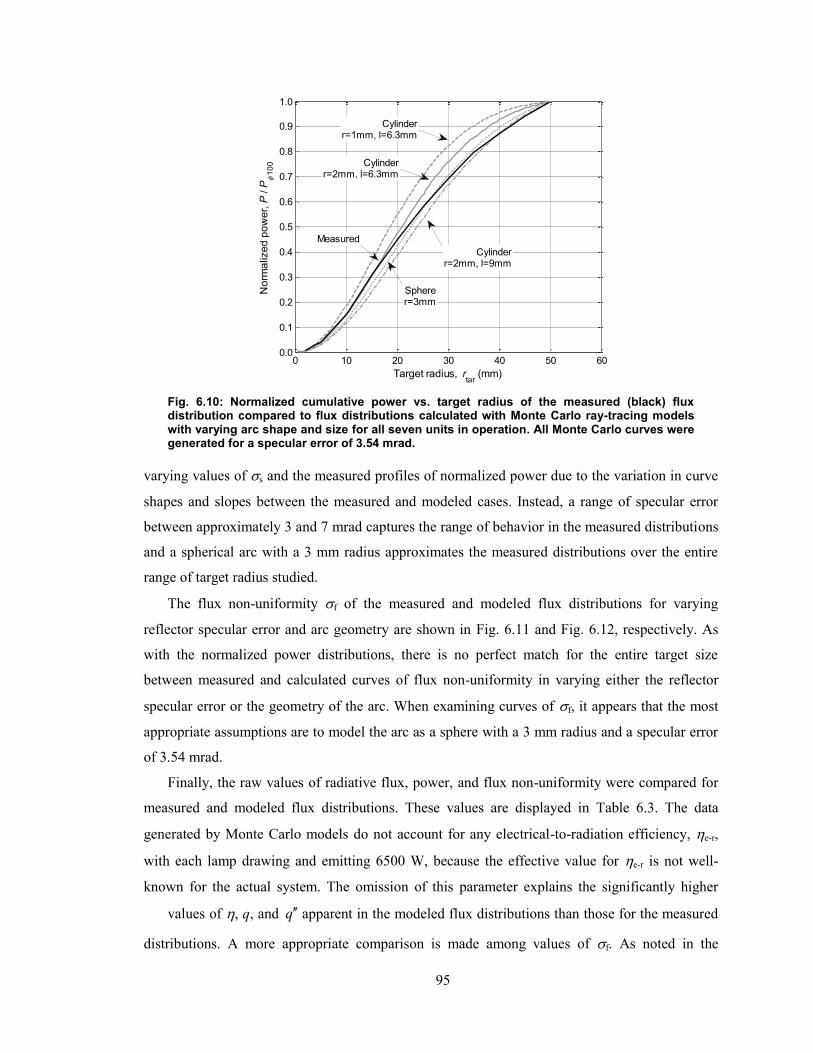
95

Fig. 6.10: Normalized cumulative power vs. target radius of the measured (black) flux distribution compared to flux distributions calculated with Monte Carlo ray-tracing models with varying arc shape and size for all seven units in operation. All Monte Carlo curves were generated for a specular error of 3.54 mrad.

varying values of s and the measured profiles of normalized power due to the variation in curve

shapes and slopes between the measured and modeled cases. Instead, a range of specular error

between approximately 3 and 7 mrad captures the range of behavior in the measured distributions

and a spherical arc with a 3 mm radius approximates the measured distributions over the entire

range of target radius studied.

The flux non-uniformity f of the measured and modeled flux distributions for varying

reflector specular error and arc geometry are shown in Fig. 6.11 and Fig. 6.12, respectively. As

with the normalized power distributions, there is no perfect match for the entire target size

between measured and calculated curves of flux non-uniformity in varying either the reflector

specular error or the geometry of the arc. When examining curves of f, it appears that the most

appropriate assumptions are to model the arc as a sphere with a 3 mm radius and a specular error

of 3.54 mrad.

Finally, the raw values of radiative flux, power, and flux non-uniformity were compared for

measured and modeled flux distributions. These values are displayed in Table 6.3. The data

generated by Monte Carlo models do not account for any electrical-to-radiation efficiency, e-r,

with each lamp drawing and emitting 6500 W, because the effective value for e-r is not well-

known for the actual system. The omission of this parameter explains the significantly higher

values of , q, and q apparent in the modeled flux distributions than those for the measured

distributions. A more appropriate comparison is made among values of f. As noted in the

0 10 20 30 40 50 600.0

0.1

0.2

0.3

0.4

0.5

0.6

0.7

0.8

0.9

1.0

Target radius, rtar

(mm)

No

rma

lize

d p

ow

er,

P / P

1

00

Cylinderr=2mm, l=6.3mm


Measured

Spherer=3mm

Cylinderr=2mm, l=9mm

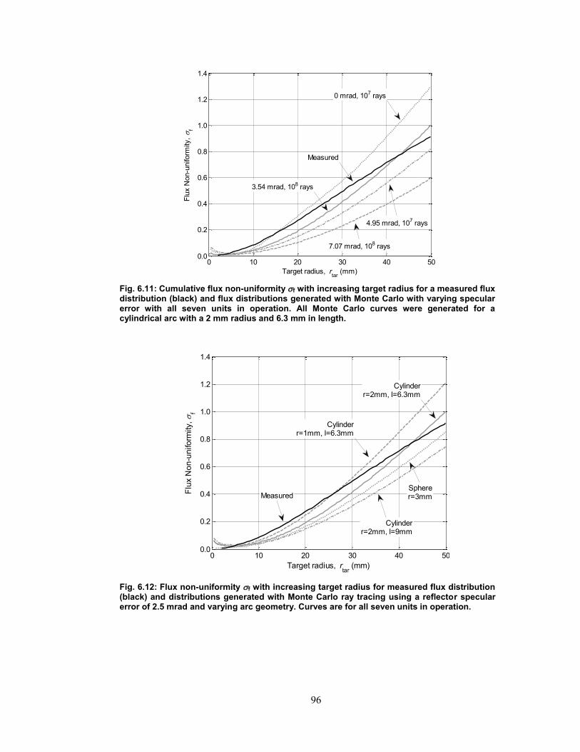
96

Fig. 6.11: Cumulative flux non-uniformity f with increasing target radius for a measured flux distribution (black) and flux distributions generated with Monte Carlo with varying specular error with all seven units in operation. All Monte Carlo curves were generated for a cylindrical arc with a 2 mm radius and 6.3 mm in length.

Fig. 6.12: Flux non-uniformity f with increasing target radius for measured flux distribution (black) and distributions generated with Monte Carlo ray tracing using a reflector specular error of 2.5 mrad and varying arc geometry. Curves are for all seven units in operation.

0 10 20 30 40 500.0

0.2

0.4

0.6

0.8

1.0

1.2

1.4

Target radius, rtar

(mm)

Flu

x N

on-u

nifo

rmity

,

f

Measured

3.54 mrad, 108 rays

7.07 mrad, 108 rays

0 mrad, 107 rays

4.95 mrad, 107 rays

0 10 20 30 40 500.0

0.2

0.4

0.6

0.8

1.0

1.2

1.4

Target radius, rtar

(mm)

Flu

x N

on

-un

ifo

rmity,

f



MeasuredSpherer=3mm

Cylinderr=2mm, l=9mm

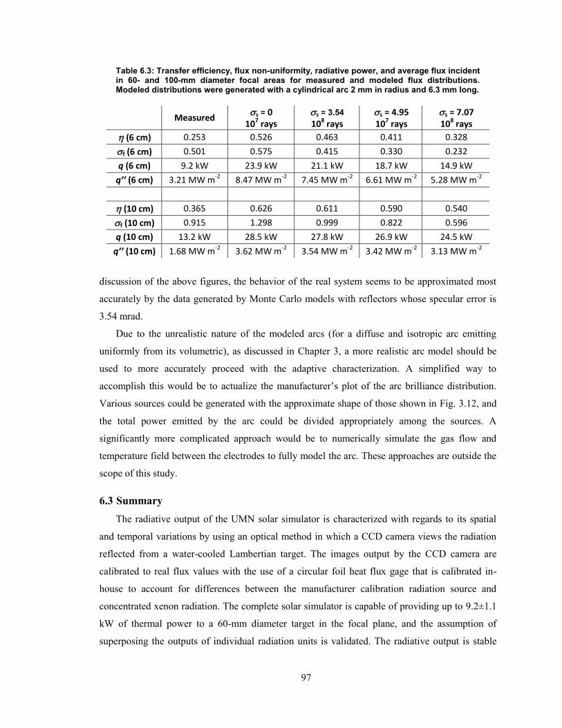
97

Table 6.3: Transfer efficiency, flux non-uniformity, radiative power, and average flux incident in 60- and 100-mm diameter focal areas for measured and modeled flux distributions. Modeled distributions were generated with a cylindrical arc 2 mm in radius and 6.3 mm long.

Measured

s = 0 107 rays

s = 3.54 108 rays

s = 4.95 107 rays

s = 7.07 108 rays

(6 cm) 0.253 0.526 0.463 0.411 0.328

f (6 cm) 0.501 0.575 0.415 0.330 0.232

q (6 cm) 9.2 kW 23.9 kW 21.1 kW 18.7 kW 14.9 kW

q’’ (6 cm) 3.21 MW m-2 8.47 MW m-2 7.45 MW m-2 6.61 MW m-2 5.28 MW m-2

(10 cm) 0.365 0.626 0.611 0.590 0.540

f (10 cm) 0.915 1.298 0.999 0.822 0.596

q (10 cm) 13.2 kW 28.5 kW 27.8 kW 26.9 kW 24.5 kW

q’’ (10 cm) 1.68 MW m-2 3.62 MW m-2 3.54 MW m-2 3.42 MW m-2 3.13 MW m-2

discussion of the above figures, the behavior of the real system seems to be approximated most

accurately by the data generated by Monte Carlo models with reflectors whose specular error is

3.54 mrad.

Due to the unrealistic nature of the modeled arcs (for a diffuse and isotropic arc emitting

uniformly from its volumetric), as discussed in Chapter 3, a more realistic arc model should be

used to more accurately proceed with the adaptive characterization. A simplified way to

accomplish this would be to actualize the manufacturer’s plot of the arc brilliance distribution.

Various sources could be generated with the approximate shape of those shown in Fig. 3.12, and

the total power emitted by the arc could be divided appropriately among the sources. A

significantly more complicated approach would be to numerically simulate the gas flow and

temperature field between the electrodes to fully model the arc. These approaches are outside the

scope of this study.

6.3 Summary

The radiative output of the UMN solar simulator is characterized with regards to its spatial

and temporal variations by using an optical method in which a CCD camera views the radiation

reflected from a water-cooled Lambertian target. The images output by the CCD camera are

calibrated to real flux values with the use of a circular foil heat flux gage that is calibrated in-

house to account for differences between the manufacturer calibration radiation source and

concentrated xenon radiation. The complete solar simulator is capable of providing up to 9.2±1.1

kW of thermal power to a 60-mm diameter target in the focal plane, and the assumption of

superposing the outputs of individual radiation units is validated. The radiative output is stable

98

after a warmup period of fifteen minutes. Although too many degrees of freedom exist in

comparing measured flux distributions to those calculated using Monte Carlo ray tracing to be

able to accurately determine the reflector specular error and effective plasma arc shape,

approximating them as s = 3.54 mrad and a sphere 3 mm in radius, respectively, provide an

adequate starting point for future calculations. More realistic models of the plasma arc, generated

by either discretizing the arc with the intensity values provided by the manufacturer (e.g., Fig.

3.12) or by a computational fluid dynamics model of the temperature field of the plasma and the

associated emission intensities. Such models are outside the scope of this work.

99

Chapter 7

Summary & Conclusions

7.1 Summary

The University of Minnesota (UMN) concentrating solar simulator provides a source of

concentrated radiation that mimics the conditions created by facilities that concentrate natural

sunlight. It is a laboratory tool that allows researchers at UMN to test and validate designs and

materials used in prototype solar thermal receivers and reactors that facilitate the generation of

solar fuels and electricity under well-controlled and repeatable conditions. The solar simulator

consists of seven commonly-focused radiation modules, each consisting of a xenon short-arc

lamp coupled to a reflector in the shape of an ellipsoid of revolution. The seven modules are

arranged in a circular pattern to maximize the symmetry of the radiation beam geometry, while

the common focal regions produces concentration ratios in excess of 3200 suns (3.2 MW m-2

). Its

design, construction, and characterization provide the basis for the present work.

The solar simulator was designed by first using geometric optics to ensure that the focal

regions of all seven lamp-reflector modules coincide, a condition which is critical in the success

of the device. A new set of unique geometric relations was developed in order to constrain the

location and orientation of each module by setting four independent parameters: the projected

orientation angle of each unit with respect to the central unit i, the truncation diameter of the

individual reflectors d, the minimum distance between the focal plane and the nearest point of a

radiation module l1, and the angle between the axis of the central module and the axis of any

peripheral module . These relations are also applicable for any odd number of modules arranged

in a circular pattern similar to that shown in Fig. 2.1 (with one central unit). The final

configuration was chosen based on both practical considerations and the requirement of matching

the radiative output of solar concentrating facilities as closely as possible, as quantified by the

beam geometry and spectral distribution. Practical considerations include reflector

manufacturability, laboratory space size, and necessary clearance allowances for mounting the

reflectors and accessing the experimental region immediately surrounding the focus. The

following conditions were chosen for the final design: a reflector truncation diameter of d = 0.75

m, minimum distance between the focal plane and the nearest point of any reflector of l1 = 1.45

m, and the angle between central and peripheral lamp axes of = 26°. The resulting rim angle

was approximately 37.7°, which is in good agreement with the requirement set in Chapter 1.

The final reflector shape was optimized by using Monte Carlo ray tracing for radiative

thermal transport to model the solar simulator and varying the reflector shape, as quantified by

100

the eccentricity of the rotated ellipse. The ray tracing analysis modeled the xenon arc as a

cylindrical source of radiation emitting isotropically, diffusely, and uniformly from its volume.

The reflectors were modeled as truncated ellipsoids of revolution with an inner surface

reflectivity of = 0.9 and specular error varying from 0 to 14.14 mrad. The target was modeled

as a flat black disk located in the focal plane, and the surroundings were non-participating (cold

and black). The reflector eccentricity was varied from 0.850 to 0.925. The goals of the

optimization study were to maximize the efficiency of energy transfer from the radiation sources

to the target while maintaining a reasonable distribution of flux in the focal plane. A trade-off in

the optimization resulted between achieving a desired flux distribution and maximizing the

delivered radiative power. Ultimately, the flux distribution was sacrificed in order to avoid a

significant loss of radiative energy delivered to the focal area. For a specular error of 7.07 mrad,

which, during the design phase, was assumed to be the most likely surface condition resulting

from the manufacturing process, the optimal eccentricity was chosen to be e = 0.890. Based on

these conditions, the solar simulator was predicted to provide 7.5 kW to a 60 mm diameter target

and a peak flux of up to 3.7 MW m-2

. After the actual flux and power were measured and

compared to simulations, it is estimated that the actual specular error of the reflectors is

somewhat lower than 7.07 mrad.

The solar simulator was fabricated according to the custom design described above. The

reflectors were constructed of spun aluminum alloy 1350 (99.5% aluminum), polished to a high

degree, and coated with quartz to deter degradation of the surface by the ultraviolet wavelengths

emitted by the lamps. Dedicated power supplies and rectifiers were installed to provide the high

DC electricity to the lamps, and several interlocks were hard-wired into the design to ensure safe

operating conditions. Kinoton GmbH was employed to construct the solar simulator and design

the electronics due to their previous experience constructing a concentrating solar simulator with

a similar concept [30]. A dedicated enclosure was designed and constructed to house the solar

simulator and protect it and researchers working in the laboratory, and is equipped with systems

to provide air and water cooling. The UMN solar simulator was installed and functioning at the

beginning of December, 2010, and was the first of its kind operating in the United States.

Accurate measurement of the solar simulator radiative output is critical in the assessment of

prototype receivers and reactors because of the crucial role the input power plays in calculating

reactor efficiency. The radiative output of the UMN solar simulator was measured with an optical

technique that is commonly used to measure the distribution of concentrated radiation output by

concentrating facilities using natural sunlight. This method involves locating a water cooled

Lambertian target in the plane of interest, while a charge-coupled device (CCD) camera views the

101

radiation reflected from the target through absorptive-reflective neutral density filters and a lens.

The grayscale photographs output by the CCD camera are calibrated to measured incident heat

flux levels by directly measuring the incident radiative flux with a circular foil heat flux gage that

is calibrated in-house. The gage was calibrated calorimetrically in-house due to the difference in

spectral and geometric distributions of the incident radiative flux generated by the simulator and

the flat black plate that was used in the gage manufacturer’s calibration. Using these

measurement techniques, the average radiative flux incident on a 60 mm diameter area in the

focal plane was measured as 3240±390 kW m-2

, corresponding to a total radiative power of

9.2±1.1 kW. The solar simulator radiative output is steady to within the measurement uncertainty

after its initial warm-up period of approximately fifteen minutes. An exact value of the reflector

specular error could not be estimated by comparing measured flux distributions to those

calculated with Monte Carlo ray tracing because of the many factors affecting the amount of

radiative power and its distribution in the focal area.

The radiative output of the resulting solar simulator reasonably matches the goal design

qualities of natural solar dish concentrators. Its peak-to-mean flux ratio over a target area 144 mm

in diameter of approximately 7.4 reasonably replicates the general conditions provided by the

EURODISH and DISTAL II parabolic dishes located at the Platforma Solar de Almería, although

the total flux and power output of the UMN simulator is less than 50% that of these particular

natural solar concentrators. The beam geometry, defined by the half angle of the cone of light

incident at the focal plane, of the designed simulator (37.7°) matches very well that of the

example solar dishes (in the range of 35–45°). Additionally, the artificial radiation source chosen

for this application (Osram XBO® 6500W/HSLA OFR) provides a relatively good match to the

solar spectrum, whose average value is quantified by the air mass 1.5 spectrum [22]. Due to these

matched results, it can be said that the UMN solar simulator reasonably replicates the radiative

output of parabolic dish concentrators of natural sunlight, but also provides extremely steady,

repeatable, and controllable conditions for experimental work.

7.2 Key Contributions

The significant contributions of this work involve the design, construction, and

characterization of the solar simulator. The unique geometric relations developed in the design

phase can be used to determine the specific location and orientation of any odd number of lamp-

reflector units, arranged with one unit in the center and an even number of units surrounding it, to

ensure that their focal points coincide. These general relations may be combined with the specific

requirements of any particular facility (including available space and manufacturability concerns)

102

to ensure correct reflector alignment and design. Additionally, the UMN high-flux solar simulator

was the first completed and operating in the United States and provides an excellent experimental

platform for laboratory-scale solar receiver and reactor testing. Finally, the detailed

characterization of the solar simulator flux output is paramount in the evaluation of the receivers

and reactors to be tested in the simulator.

7.3 Recommendations for Future Work

Further research regarding the behavior of the UMN solar simulator might include measuring

the spectral distribution of its output in the focal plane. Two reasons exist for completing this

measurement. The first deals with the possibility that the spectral distribution of the radiation

incident at the focal plane may vary depending on the measurement location relative to the ideal

focus, which could affect measurements of integrated power and average flux using the optical

method employed here, as discussed in Section 5.2.2 [58]. The second reason for measuring the

spectral distribution would be to determine the spectral distribution at wavelengths longer than

those presented by the bulb manufacturer for better estimation of the gage’s effective total

hemispherical absorptivity.

Measurement of the concentrated radiative energy spectrum in the focal plane is necessary in

determining whether the effect observed by Alxneit and Schmit [58] are also present in the UMN

solar simulator. As discussed in Section 5.2.2, spectral distributions varying within the focal

plane may affect optical measurements due to the spectral sensitivity of the filters, lens, and

camera. Although preliminary calculations using published data indicate that such errors are less

than 1%, measurements of the concentrated flux spectral intensity at various locations in the focal

plane would provide the basis for a more accurate estimation of these errors.

Although the total hemispherical absorptivity of the heat flux gage has been estimated by

weighting the measured spectral hemispherical absorptivity with the spectral distribution

provided by the lamp manufacturer [42], the provided distribution is limited to a wavelength

range of 250–1650 nm. It has been shown for similar lamps drawing less power that up to 30%

more energy is present in the farther infrared wavelengths [59] that is unaccounted for in the

present work. If data are measured at longer wavelengths, a more complete estimate of the gage’s

absorptivity would be possible, increasing the confidence of the thermal balance calibration

method.

In order to avoid the effects of possible calibration errors in the optical flux measurement

method due to spatial-spectral variations or heat flux gage calibration errors, it is recommended

that concomitant measurements of concentrated flux are taken using a fluid calorimeter. A fluid

103

calorimeter generally consists of a water-cooled cavity, either in a closed or open system. When

the energy absorbed by the water, the absorptivity of the cavity, and the aperture area are well-

characterized, the incident radiative flux and power integrated over the aperture area are directly

related to primary measurements [73–76].

One further tool that would be useful in designing future prototype receivers and reactors to

be tested in the UMN solar simulator is a three-dimensional characterization and reconstruction

of the resulting directional radiative intensity. Radiative transport within receiver and reactive

cavities strongly depends on the directional distribution of the incoming rays, so this information

may be critical to accurate predictions of prototype behaviors and useful in cavity design.

Erickson and Petrasch have developed a method to successfully reconstruct the intensity

distribution in two dimensions, but further work is required to expand the technique to three-

dimensional use [77].

104

Bibliography

[1] Denton J. C., 1977, “Solar power system,” Energy Conversion, 16(4), pp. 181-198.

[2] Steinfeld A., and Palumbo R. D., 2001, “SOLAR THERMOCHEMICAL PROCESS

TECHNOLOGY,” Encyclopedia of Physial Science & Technology, 15, pp. 237-256.

[3] Fletcher E. a., 2001, “Solarthermal Processing: A Review,” Journal of Solar Energy

Engineering, 123(2), pp. 63-74.

[4] Kodama T., 2003, “High-temperature solar chemistry for converting solar heat to

chemical fuels,” Progress in Energy and Combustion Science, 29(6), pp. 567-597.

[5] Wilhelm D., 2001, “Syngas production for gas-to-liquids applications: technologies, issues

and outlook,” Fuel Processing Technology, 71(1-3), pp. 139-148.

[6] Steinfeld A., 1998, “A solar chemical reactor for co-production of zinc and synthesis gas,”

Energy, 23(10), pp. 803-814.

[7] Gregg D., Taylor R., Campbell J., Taylor J., and Cotton A., 1980, “Solar gasification of

coal, activated carbon, coke and coal and biomass mixtures,” Solar Energy, 25(4), pp.

353-364.

[8] Stine W. B., and Diver R. B., 1994, A compendium of solar dish/Stirling technology.

[9] Mills D., 2004, “Advances in solar thermal electricity technology,” Solar Energy, 76(1-3),

pp. 19-31.

[10] Müller-Steinhagen H., 2004, “Solar Power,” Quarterly of the Royal Academy of

Engineering, pp. 43-50.

[11] Thomas A., and Guven H. M., 1993, “Parabolic trough concentrators design construction

and evaluation,” Energy Conversion, 34(5), pp. 401-416.

[12] Segal A., and Epstein M., 2001, “The optics of the solar tower reflector,” Solar Energy,

69, pp. 229-241.

[13] Haueter P., Seitz T., and Steinfeld A., 1999, “A New high-flux solar furnace for high-

temperature thermochemical research,” Journal of Solar Energy Engineering,

121(February), pp. 77-80.

[14] Ulmer S., Reinalter W., Heller P., L pfert E., and Mart nez D., 2002, “Beam

Characterization and Improvement with a Flux Mapping System for Dish Concentrators,”

Journal of Solar Energy Engineering, 124(2), pp. 182-188.

[15] Schubnell M., and Keller J., 1991, “Flux density distribution in the focal region of a solar

concentrator system,” Journal of solar energy engineering, 113, pp. 112-116.

105

[16] L pfert E., Monterreal R., Heller P., and Reche J. F., 2000, “Concentrated solar radiation

measurement with video image processing and online fluxgage calibration,” Proc. of 10th

SolarPACES Int. Symp. Solar Thermal, pp. 8–10.

[17] National Renewable Energy Laboratory, 2010, “Parabolic Trough Power Plant System

Technology,” Parabolic Trough Solar Power Network.

[18] Kearney D. W., 2007, “Parabolic Trough Collector Overview.”

[19] Burroughs C., and Hecker L., 2008, “Sandia, Stirling Energy Systems set new world

record for solar-to-grid conversion efficiency,” Sandia News Release.

[20] Southwest Solar Technologies, “Solar Dish.”

[21] Abengoa Solar S.A., 2011, “Operating Facilities: Spain,” Abengoa Solar: Our Plants.

[22] Gueymard C., 2002, “Proposed reference irradiance spectra for solar energy systems

testing,” Solar Energy, 73(6), pp. 443-467.

[23] Shuai Y., Xia X., and Tan H., 2008, “Radiation performance of dish solar

concentrator/cavity receiver systems,” Solar Energy, 82(1), pp. 13-21.

[24] Beattie W. H., Berjoan R., and Coutures J.-P., 1983, “HIGH-TEMPERATURE SOLAR

PYROLYSIS OF COAL,” Solar Energy, 31(2), pp. 137-143.

[25] Bartera R. E., Riise H. N., and Miller C. G., 1970, “Solar Simulators at the Jet Propulsion

Laboratory,” Applied Optics, 9(5), pp. 1068-1074.

[26] Jefferies K. S., 1994, Solar Simulator for Solar Dynamic Space Power System Testing,

Cleveland, Ohio.

[27] Kuhn P., and Hunt A., 1991, “A new solar simulator to study high temperature solid-state

reactions with highly concentrated radiation,” Solar Energy Materials, 24, pp. 742-750.

[28] Hirsch D., Zedtwitz P. V., Osinga T., Kinamore J., and Steinfeld A., 2003, “A New 75 kW

High-Flux Solar Simulator for High-Temperature Thermal and Thermochemical

Research,” Journal of Solar Energy Engineering, 125(1), pp. 117-120.

[29] Petrasch J., Coray P., Meier A., Brack M., H berling P., Wuillemin D., and Steinfeld A.,

2007, “A Novel 50 kW 11,000 suns High-Flux Solar Simulator Based on an Array of

Xenon Arc Lamps,” Journal of Solar Energy Engineering, 129(4), pp. 405-411.

[30] DLR Institute of Solar Research, 2012, “High-Flux Solar Furnace and Xenon-High-Flux

Solar Simulator.”

[31] Florida Energy Systems Consortium, 2008, “Solar to Fuel.”

106

[32] Krueger K. R., Davidson J. H., and Lipiński W., 2011, “Design of a New 45 kWe High-

Flux Solar Simulator for High-Temperature Solar Thermal and Thermochemical

Research,” Journal of Solar Energy Engineering, 133(1), p. 011013.

[33] Krueger K. R., Davidson J. H., and Lipiński W., 2012, “Operational Performance of the

University of Minnesota 45kWe High-Flux Solar Simulator,” ASME 2012 6th

International Conference on Energy Sustainability & 10th Fuel Cell Science, Engineering

and Technology Conference.

[34] Petrasch J., Takagi M., and Erickson B., 2011, “Thrust Area 4 : Solar (Thermal) Solar

Fuels from Thermochemical Cycles at Low Pressures,” (July), pp. 152-156.

[35] Neumann A., and Groer U., 1996, “Experimenting with Concentrated Sunlight Using the

DLR Solar Furnace,” Solar Energy, 58(4), pp. 181-190.

[36] Thalhammer E., 1979, “Heliostat beam characterization system––update,” ISA/79 Conf.

Proc., Chicago, IL, USA, pp. 505-521.

[37] Strachan J. W., 1993, “Revisiting the BCS, a measurement system for characterizing the

optics of solar collectors,” pp. 797-808.

[38] Kenny S. P., and Davidson J. H., 1994, “Design of a Multiple-Lamp Large-Scale Solar

Simulator,” Journal of Solar Energy Engineering, 116(November), pp. 200-205.

[39] Domínguez C., Antón I., and Sala G., 2008, “Solar simulator for concentrator photovoltaic

systems.,” Optics express, 16(19), pp. 14894-901.

[40] Seckmeyer G., and Payer H.-D., 1993, “A new sunlight simulator for ecological research

on plants,” Journal of Photochemistry and Photobiology B: Biology, 21, pp. 175-181.

[41] Hinczewski D. S., Hinczewski M., Tepehan F. Z., and Tepehan G. G., 2005, “Optical

filters from SiO2 and TiO2 multi-layers using sol–gel spin coating method,” Solar Energy

Materials and Solar Cells, 87(1-4), pp. 181-196.

[42] Osram GmbH, “Manufacturer Data.”

[43] Steinfeld A., “Exchange factor between two spheres placed at the foci of a specularly

reflecting ellipsoidal cavity,” International communications in heat and mass transfer,

18(1), pp. 19-26.

[44] Osram GmbH, 2008, “HMI (R) 6000 W/SE XS.”

[45] Guesdon C., Alxneit I., Tschudi H. R., Wuillemin D., and Sturzenegger M., 2006, “1 kW

imaging furnace with in situ measurement of surface temperature,” Review of Scientific

Instruments, 77(3), p. 035102.

[46] Petrasch J., 2010, “A Free and Open Source Monte Carlo Ray Tracing Program for

Concentrating Solar Energy Research,” Proceedings of the ASME 2010 4th International

Conference on Energy Sustainability, Phoenix, AZ, pp. 125-132.

107

[47] Howell J. R., 1998, “The Monte Carlo Method in Radiative Heat Transfer,” Journal of

Heat Transfer, 120(3), pp. 547-560.

[48] Modest M. F., 2003, “The Monte Carlo Method for Thermal Radiation,” Radiative Heat

Transfer, Elsevier Science (USA), San Diego, California, USA, pp. 644 - 679.

[49] Kalos M. H., and Whitlock P. A., 2008, Monte Carlo Methods, Wiley-VCH, Weinheim.

[50] Siegel R., and Howell J. R., 1992, Thermal Radiation Heat Transfer, Taylor & Francis

Ltd., Philadelphia, PA.

[51] Osram, “XBO® – theater lamps. Technology and Application,” Technology.

[52] UMN Facilities Management, 2012, “Internal Architectural Data.”

[53] Ballestrín J., Rodríguez-Alonso M., Rodriguez J., Cañadas I., Barbero F., Langley L. W.,

and Barnes A., 2006, “Calibration of high-heat-flux sensors in a solar furnace,”

Metrologia, 43(6), pp. 495-500.

[54] Gardon R., 1953, “An Instrument for the Direct Measurement of Intense Thermal

Radiation,” Review of Scientific Instruments, 24(5), pp. 366-70.

[55] Vatell Corporation, 2011, “Vatell Calibration Procedures.”

[56] Stagg B. J., and Charalampopoulos T. T., 1993, “Refractive Indices of Pyrolytic Graphite ,

Amorphous Carbon , and Flame Soot in the Temperature Range 25 ° to 600 ° C,” 396, pp.

381-396.

[57] Peatross J., and Ware M., 2011, Physics of light and optics, Brigham Young University.

[58] Alxneit I., and Schmit H., 2012, “Spectral Characterization of PSI’s High-Flux Solar

Simulator,” Journal of Solar Energy Engineering, 134(1), p. 011013.

[59] Nakar D., Malul A., Feuermann D., and Gordon J. M., 2008, “Radiometric

characterization of ultrahigh radiance xenon short-arc discharge lamps.,” Applied optics,

47(2), pp. 224-229.

[60] PENTAX Corporation, 2011, Technical Data.

[61] CVA Melles Griot, 2012, SPECIFICATIONS : Metallic Neutral Density Filters.

[62] Basler Inc., 2007, Basler scA1400-17fm Camera Specification, Exton, PA.

[63] Kaluza J., and Neumann A., 2001, “Comparative Measurements of Different Solar Flux

Gauge Types,” Journal of Solar Energy Engineering, 123(3), pp. 251-255.

[64] Ballestrín J., Ulmer S., Morales A., Barnes A., Langley L. W., and Rodríguez M., 2003,

“Systematic error in the measurement of very high solar irradiance,” Solar Energy

Materials and Solar Cells, 80(3), pp. 375-381.

108

[65] Touloukian Y. S., and Dewitt D. P., 1972, Thermal radiative properties: Nonmetallic

solids.

[66] Ballestrín J., Estrada C. A., Rodríguez-Alonso M., Pérez-Rábago C. a., Langley L. W.,

and Barnes A., 2004, “High-heat-flux sensor calibration using calorimetry,” Metrologia,

41(4), pp. 314-318.

[67] Ballestrín J., Estrada C. A., Rodríguez-Alonso M., Pérez-Rábago C. a., Langley L. W.,

and Barnes A., 2006, “Heat flux sensors: Calorimeters or radiometers?,” Solar Energy,

80(10), pp. 1314-1320.

[68] Fried E., 1969, “Thermal Conduction Contribution to Heat Transfer at Contacts,” Thermal

Conductivity, Vol. 2, R.P. Tye, ed., Academic Press, Inc., London; New York, pp. 253-

274.

[69] National Instruments, 2010, “Perspective and Nonlinear Distortion Calibration,” NI

Vision 2010 for LabVIEW Help.

[70] Coray P., 2009, “Perspective transformation algorithm,” (October 2007), pp. 1-13.

[71] Coray P., 2008, “Total Flux.”

[72] Figliola R. S., and Beasley D. E., 2000, Theory and Design for Mechanical Measurements,

John Wiley & Sons, New York, NY.

[73] Diver R. B., Carlson D. E. E., Macdonald F. J., and Fletcher E. a., 1983, “A New High-

Temperature Solar Research Furnace,” Journal of Solar Energy Engineering, 105(3), pp.

288-293.

[74] Pérez-Rábago C. a., Marcos M. J., Romero M., and Estrada C. A., 2006, “Heat transfer in

a conical cavity calorimeter for measuring thermal power of a point focus concentrator,”

Solar Energy, 80(11), pp. 1434-1442.

[75] Willoughby a. B., 1954, “Absolute Water Flow Calorimeter for the Measurement of

Intense Beams of Radiant Energy,” Review of Scientific Instruments, 25(7), pp. 667-670.

[76] Estrada C. A., Jaramillo O. a., Acosta R., and Arancibia-Bulnes C. a., 2007, “Heat transfer

analysis in a calorimeter for concentrated solar radiation measurements,” Solar Energy,

81(10), pp. 1306-1313.

[77] Erickson B., and Petrasch J., 2012, “Inverse identification of intensity distributions from

multiple flux maps in concentrating solar applications,” Eurotherm Seminar 95.

[78] Kline S., and McClintock F. A., 1953, “Describing uncertainties in single-sample

experiments,” Mechanical engineering, 75(1), pp. 3-8.

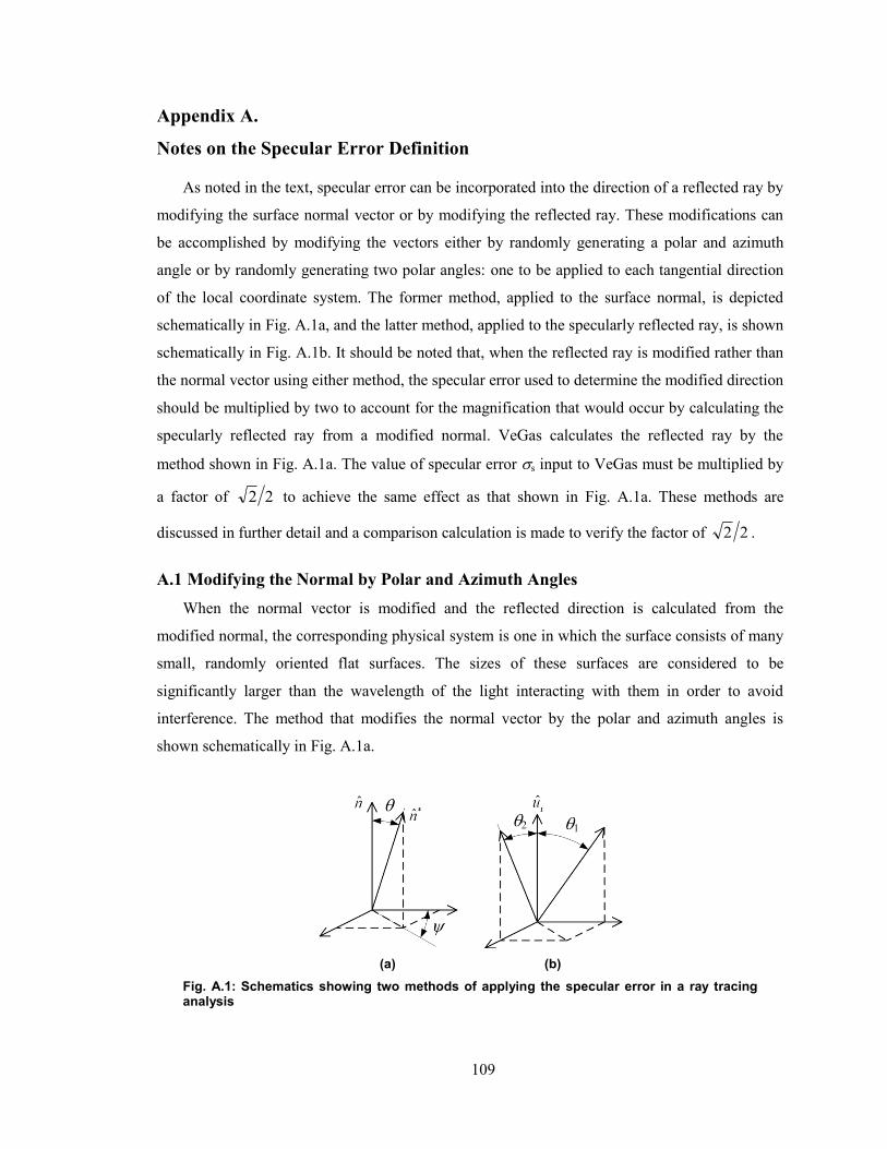
109

Appendix A.

Notes on the Specular Error Definition

As noted in the text, specular error can be incorporated into the direction of a reflected ray by

modifying the surface normal vector or by modifying the reflected ray. These modifications can

be accomplished by modifying the vectors either by randomly generating a polar and azimuth

angle or by randomly generating two polar angles: one to be applied to each tangential direction

of the local coordinate system. The former method, applied to the surface normal, is depicted

schematically in Fig. A.1a, and the latter method, applied to the specularly reflected ray, is shown

schematically in Fig. A.1b. It should be noted that, when the reflected ray is modified rather than

the normal vector using either method, the specular error used to determine the modified direction

should be multiplied by two to account for the magnification that would occur by calculating the

specularly reflected ray from a modified normal. VeGas calculates the reflected ray by the

method shown in Fig. A.1a. The value of specular error s input to VeGas must be multiplied by

a factor of 22 to achieve the same effect as that shown in Fig. A.1a. These methods are

discussed in further detail and a comparison calculation is made to verify the factor of 22 .

A.1 Modifying the Normal by Polar and Azimuth Angles

When the normal vector is modified and the reflected direction is calculated from the

modified normal, the corresponding physical system is one in which the surface consists of many

small, randomly oriented flat surfaces. The sizes of these surfaces are considered to be

significantly larger than the wavelength of the light interacting with them in order to avoid

interference. The method that modifies the normal vector by the polar and azimuth angles is

shown schematically in Fig. A.1a.

(a) (b)

Fig. A.1: Schematics showing two methods of applying the specular error in a ray tracing analysis

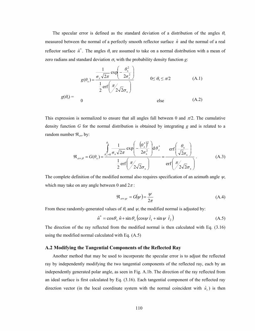
110

The specular error is defined as the standard deviation of a distribution of the angles s

measured between the normal of a perfectly smooth reflector surface n and the normal of a real

reflector surface .ˆ*n The angles s are assumed to take on a normal distribution with a mean of

zero radians and standard deviation s with the probability density function g:

g(s) =

s

2

2s

s

22erf

2

1

2exp

2

1

)(

ssσ

θ

σθg 0≤ s ≤ /2 (A.1)

0 else (A.2)

This expression is normalized to ensure that all angles fall between 0 and /2. The cumulative

density function G for the normal distribution is obtained by integrating g and is related to a

random number err by:

.

22erf

2erf

22erf

2

1

d2

exp2

1

)(

s

s

s

s

*

0

2s

2*

s

s,

s

*

σ

θθ

σ

θ

σθG

s

θ

θ

s

errs (A.3)

The complete definition of the modified normal also requires specification of an azimuth angle ,

which may take on any angle between 0 and 2 :

2, Gerr (A.4)

From these randomly-generated values of s and , the modified normal is adjusted by:

21ss* ˆsinˆcossinˆcosˆ ttnn (A.5)

The direction of the ray reflected from the modified normal is then calculated with Eq. (3.16)

using the modified normal calculated with Eq. (A.5)

A.2 Modifying the Tangential Components of the Reflected Ray

Another method that may be used to incorporate the specular error is to adjust the reflected

ray by independently modifying the two tangential components of the reflected ray, each by an

independently generated polar angle, as seen in Fig. A.1b. The direction of the ray reflected from

an ideal surface is first calculated by Eq. (3.16). Each tangential component of the reflected ray

direction vector (in the local coordinate system with the normal coincident with ru ) is then

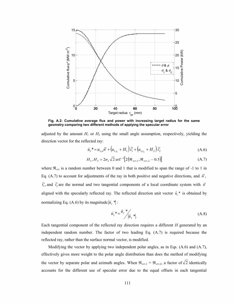
111

Fig. A.2: Cumulative average flux and power with increasing target radius for the same geometry comparing two different methods of applying the specular error

adjusted by the amount H1 or H2 using the small angle assumption, respectively, yielding the

direction vector for the reflected ray:

22,r11,r,rrˆˆˆ*

21tHutHunuu ttn

(A.6)

5.0,2erf22, 2,1,1

s21 errerrσHH (A.7)

where err is a random number between 0 and 1 that is modified to span the range of -1 to 1 in

Eq. (A.7) to account for adjustments of the ray in both positive and negative directions, and ,n

,1t and 2t are the normal and two tangential components of a local coordinate system with nˆ

aligned with the specularly reflected ray. The reflected direction unit vector *ˆru is obtained by

normalizing Eq. (A.6) by its magnitude *ru

:

.*

**

r

rr u

uu

(A.8)

Each tangential component of the reflected ray direction requires a different H generated by an

independent random number. The factor of two leading Eq. (A.7) is required because the

reflected ray, rather than the surface normal vector, is modified.

Modifying the vector by applying two independent polar angles, as in Eqs. (A.6) and (A.7),

effectively gives more weight to the polar angle distribution than does the method of modifying

the vector by separate polar and azimuth angles. When err,1 = err,2, a factor of 2 identically

accounts for the different use of specular error due to the equal offsets in each tangential

0 20 40 60 80 1000

5

10

15

Cu

mu

lative

flu

x q

" (M

W m

-2)

0 20 40 60 80 1000

5

10

15

20

25

30

Cu

mu

lative

Po

we

r (k

W)

Target radius rtar

(mm)

&

1 &

2

112

direction. For the majority of the cases in which err,1 ≠ err,2, the different uses of specular error

are nevertheless captured by incorporating the factor of 2 . Two full simulator models with

identical geometry (e=0.890) but different methods of calculating s were run and the resulting

curves of average flux and cumulative power are shown in Fig. A.2. Both cases accounted for the

specular error by modifying the reflected vector; the dashed curve, labeled “ & ”, adjusted the

polar and azimuth angles, while the solid curve, labeled “1 & 2”, modified the reflected vector

by its two tangential components, as described above. Whereas the “1 & 2” model applied a

specular error of 2.5 mrad, the “ & ” model applied a specular error of 3.54 mrad. The very

close overlap of these curves shows that the factor of 2 adequately accounts for the different

methods.

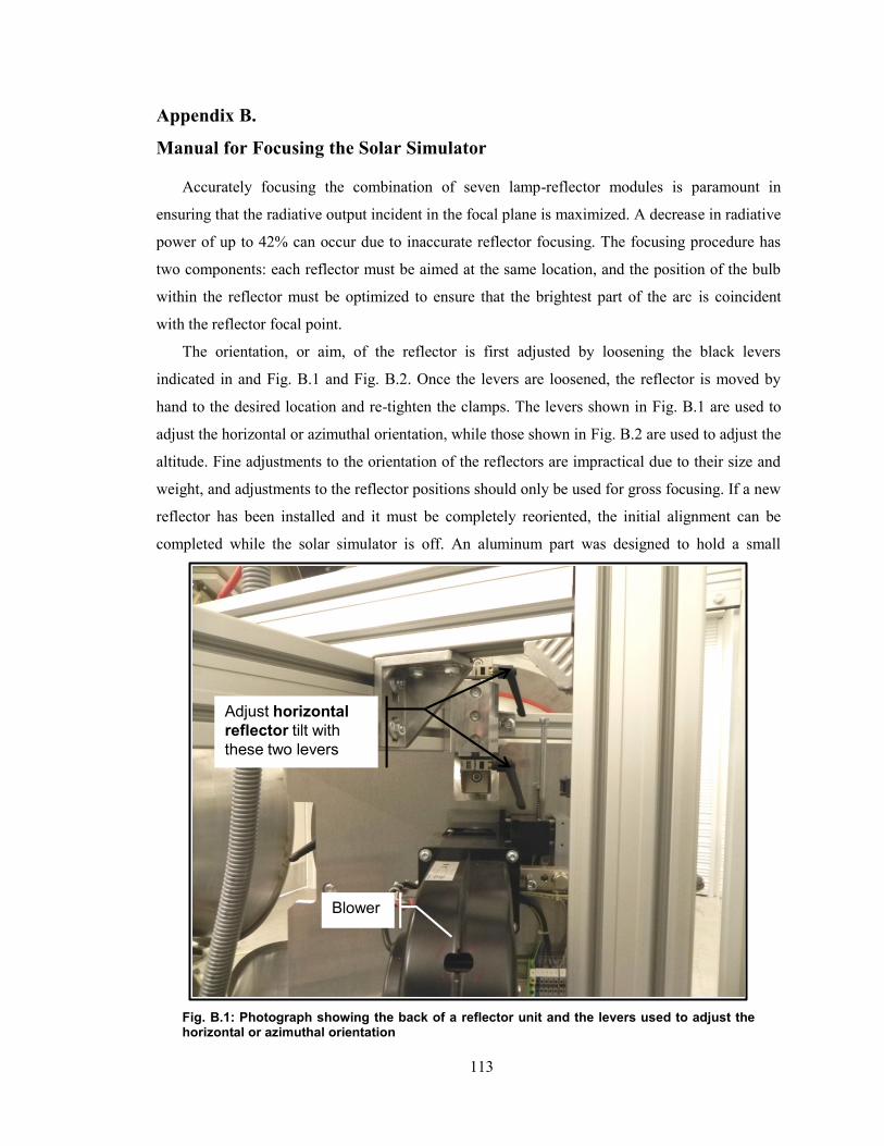
113

Appendix B.

Manual for Focusing the Solar Simulator

Accurately focusing the combination of seven lamp-reflector modules is paramount in

ensuring that the radiative output incident in the focal plane is maximized. A decrease in radiative

power of up to 42% can occur due to inaccurate reflector focusing. The focusing procedure has

two components: each reflector must be aimed at the same location, and the position of the bulb

within the reflector must be optimized to ensure that the brightest part of the arc is coincident

with the reflector focal point.

The orientation, or aim, of the reflector is first adjusted by loosening the black levers

indicated in and Fig. B.1 and Fig. B.2. Once the levers are loosened, the reflector is moved by

hand to the desired location and re-tighten the clamps. The levers shown in Fig. B.1 are used to

adjust the horizontal or azimuthal orientation, while those shown in Fig. B.2 are used to adjust the

altitude. Fine adjustments to the orientation of the reflectors are impractical due to their size and

weight, and adjustments to the reflector positions should only be used for gross focusing. If a new

reflector has been installed and it must be completely reoriented, the initial alignment can be

completed while the solar simulator is off. An aluminum part was designed to hold a small

Fig. B.1: Photograph showing the back of a reflector unit and the levers used to adjust the horizontal or azimuthal orientation

Adjust horizontal

reflector tilt with

these two levers

Blower

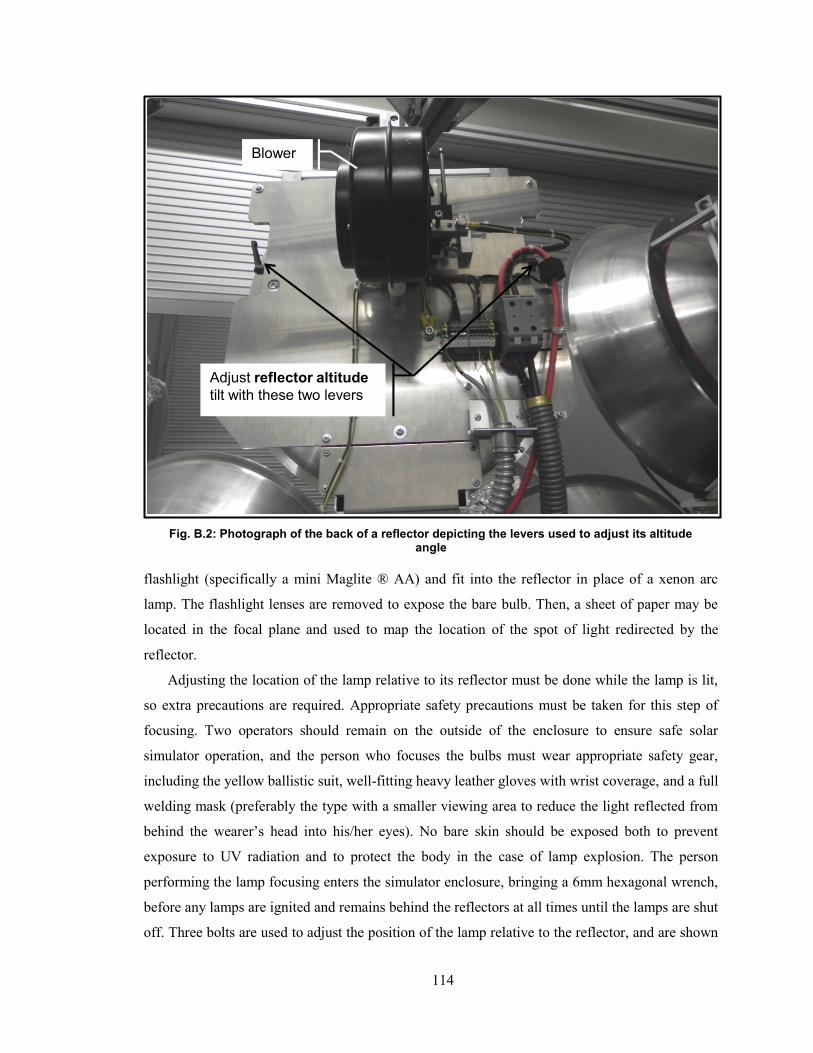
114

Fig. B.2: Photograph of the back of a reflector depicting the levers used to adjust its altitude angle

flashlight (specifically a mini Maglite ® AA) and fit into the reflector in place of a xenon arc

lamp. The flashlight lenses are removed to expose the bare bulb. Then, a sheet of paper may be

located in the focal plane and used to map the location of the spot of light redirected by the

reflector.

Adjusting the location of the lamp relative to its reflector must be done while the lamp is lit,

so extra precautions are required. Appropriate safety precautions must be taken for this step of

focusing. Two operators should remain on the outside of the enclosure to ensure safe solar

simulator operation, and the person who focuses the bulbs must wear appropriate safety gear,

including the yellow ballistic suit, well-fitting heavy leather gloves with wrist coverage, and a full

welding mask (preferably the type with a smaller viewing area to reduce the light reflected from

behind the wearer’s head into his/her eyes). No bare skin should be exposed both to prevent

exposure to UV radiation and to protect the body in the case of lamp explosion. The person

performing the lamp focusing enters the simulator enclosure, bringing a 6mm hexagonal wrench,

before any lamps are ignited and remains behind the reflectors at all times until the lamps are shut

off. Three bolts are used to adjust the position of the lamp relative to the reflector, and are shown

Adjust reflector altitude

tilt with these two levers

Blower

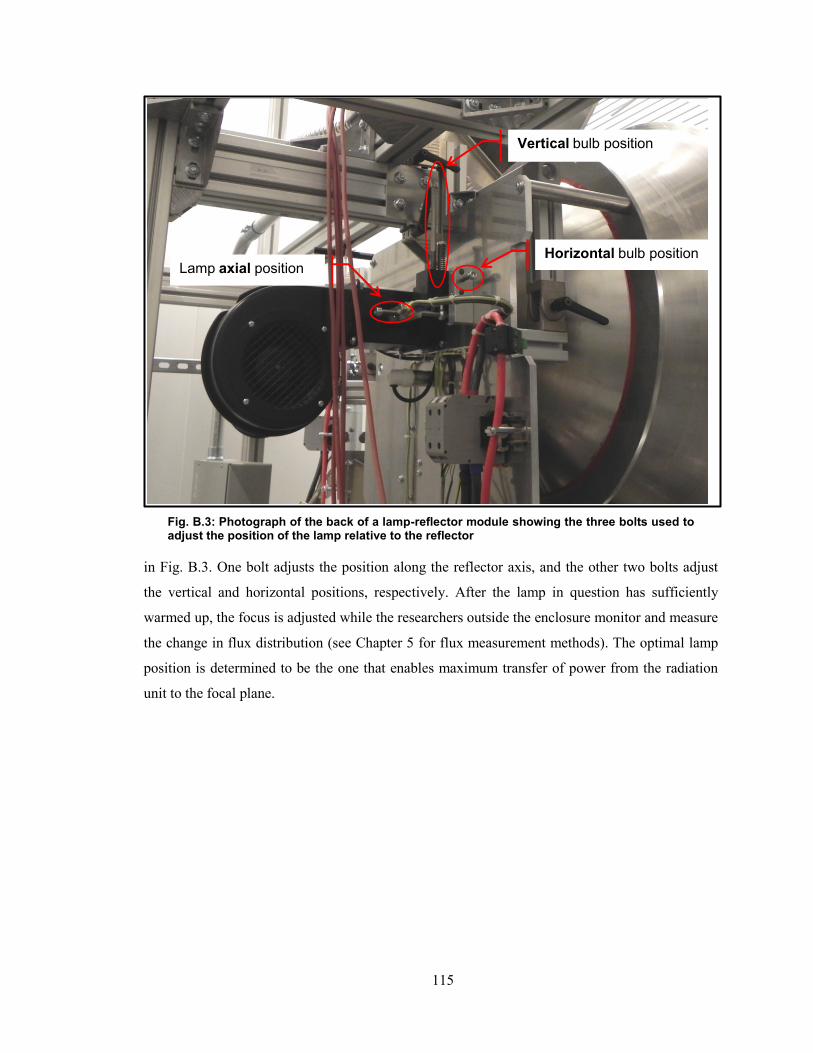
115

Fig. B.3: Photograph of the back of a lamp-reflector module showing the three bolts used to adjust the position of the lamp relative to the reflector

in Fig. B.3. One bolt adjusts the position along the reflector axis, and the other two bolts adjust

the vertical and horizontal positions, respectively. After the lamp in question has sufficiently

warmed up, the focus is adjusted while the researchers outside the enclosure monitor and measure

the change in flux distribution (see Chapter 5 for flux measurement methods). The optimal lamp

position is determined to be the one that enables maximum transfer of power from the radiation

unit to the focal plane.

Vertical bulb position

Horizontal bulb positionLamp axial position

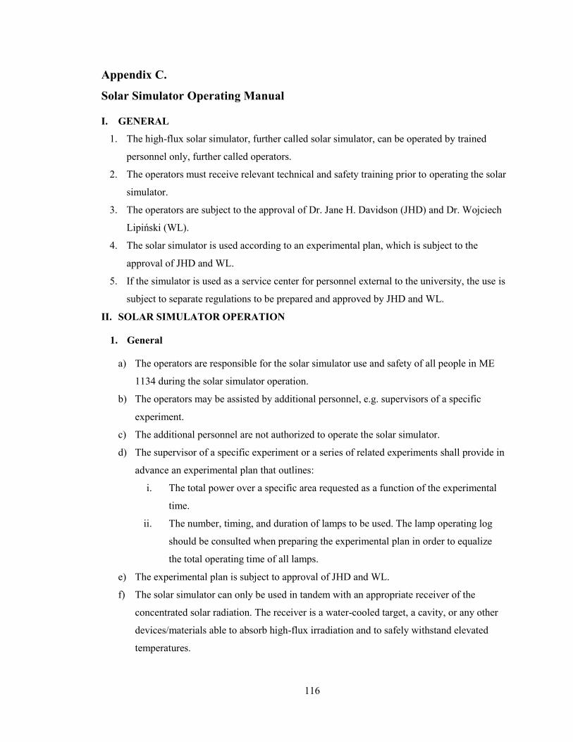
116

Appendix C.

Solar Simulator Operating Manual

I. GENERAL

1. The high-flux solar simulator, further called solar simulator, can be operated by trained

personnel only, further called operators.

2. The operators must receive relevant technical and safety training prior to operating the solar

simulator.

3. The operators are subject to the approval of Dr. Jane H. Davidson (JHD) and Dr. Wojciech

Lipiński (WL).

4. The solar simulator is used according to an experimental plan, which is subject to the

approval of JHD and WL.

5. If the simulator is used as a service center for personnel external to the university, the use is

subject to separate regulations to be prepared and approved by JHD and WL.

II. SOLAR SIMULATOR OPERATION

1. General

a) The operators are responsible for the solar simulator use and safety of all people in ME

1134 during the solar simulator operation.

b) The operators may be assisted by additional personnel, e.g. supervisors of a specific

experiment.

c) The additional personnel are not authorized to operate the solar simulator.

d) The supervisor of a specific experiment or a series of related experiments shall provide in

advance an experimental plan that outlines:

i. The total power over a specific area requested as a function of the experimental

time.

ii. The number, timing, and duration of lamps to be used. The lamp operating log

should be consulted when preparing the experimental plan in order to equalize

the total operating time of all lamps.

e) The experimental plan is subject to approval of JHD and WL.

f) The solar simulator can only be used in tandem with an appropriate receiver of the

concentrated solar radiation. The receiver is a water-cooled target, a cavity, or any other

devices/materials able to absorb high-flux irradiation and to safely withstand elevated

temperatures.

117

g) The red internal safety switch must remain in the off (down) position at all times when

the simulator is not actively in use.

h) The interior overhead door (shutter) must remain closed for any activity in the

experimental area requiring human presence and taking longer than 5 minutes.

i) Do not use the solar simulator if the room air temperature is higher than 80°F (27°C)

j) The main enable key is always removed from the panel and stored in the controls

electronics cabinet when the solar simulator is not in use.

k) Only the solar simulator operators are allowed to enter the solar simulator enclosure

when the internal overhead door (shutter) is open.

l) Never enter / try to enter the solar simulator enclosure when any lamp is on.

2. Preliminary checks and experiment preparation

a) Measure the temperature of the room air using the display mounted to the right of the

control panel. Do not use the simulator if the room air temperature is higher than 80°F

(27°C).

b) Verify that the room HVAC is online by feeling for flow from an HVAC vent.

c) Ensure that the ventilation openings at the back wall of the solar simulator enclosure are

unobstructed.

d) Turn on the PC system (conrad.me.umn.edu, located next to the control panel on the east

enclosure wall).

e) Distribute protective eyewear to everyone in the lab (clear plastic safety glasses are

located in the top of the red tool chest). These limit the exposure of UV radiation to

personnel’s eyes. Also have at least one each of a black welding mask and a clear face

shield at close reach (they are located in the left-hand gray cabinet in the northeast corner

of ME 1134, near the fume hood).

f) Position the receiver setup (target, cavity, or other receiving device/material) in the focal

area. An “X” is marked on the floor in orange tape that represents the ideal focal point,

and the vertical position can be obtained by the ideal focal height of 1289 mm (2 ft 2.75

in).

g) Open the “Total_Flux” executable (shortcut on the desktop of conrad.me.umn.edu).

Verify communication with the CCD camera by navigating to the “Camera” tab and

clicking on the activation toggle switch (see Fig. C.1). If an error window appears that

reads “Camera not found,” the camera is not communicating with the PC. Troubleshoot

as follows:

118

Fig. C.1: Screen shot of the flux measurement software (T-Flux) used to view the CCD camera output

i. Put on a clear face mask, open the swinging entry door, enter the test enclosure,

and turn off the interior safety switch (down position).

ii. Enter the simulator lamp enclosure and disconnect and re-connect the gigabit

Ethernet and power connections to the back of the camera.

iii. Turn on the interior safety switch and exit the test enclosure. Close and lock the

man door.

h) Ensure that the camera and filter are ready for operation of the solar simulator. Do this by

activating the camera through the T-Flux software. Turn on Live View in T-Flux. If static

appears when no lamps are lit, the filters are properly mounted. WARNING: DO NOT

turn on any lamps when a filter or lens cap does not cover the camera lens. Exposing the

camera’s CCD chip to unfiltered concentrated light will irreparably damage the camera.

i) If cooling water will be used, launch the cooling water temperature measurement

application (e.g, “SingleChan_Temp.vi”), which can be found on the PC desktop.

SingleChan_Temp.vi is a simple program that monitors and displays the temperature of a

thermocouple connected to channel 8 on the SCXI-1102 thermocouple card.

j) Turn on the cooling water for the receiver setup (from the sink or the installed chilled

water lines).

Activation

Live View

119

i. Check for leaks from the cooling water circuit visually by looking for dripping

water, and manually by feeling connections for moisture.

ii. If condensation on the receiver equipment is problematic, measure and monitor

the cooling water temperature at the receiver inlet. Use the Omega RH70

hygrometer (kept in a blue plastic box) to determine the dew point of the room

air. If the dew point temperature of the room air is higher than that of the cooling

water at the receiver inlet, moisture will condense on the receiver equipment.

iii. Measure and monitor the temperature of the cooling water at the outlet of the

receiver with a thermocouple connected to the SCXI data acquisition system, as

close to the receiver as possible, to ensure that it reaches no more than 158°F

(70°C) during operation. Boiling should absolutely be avoided.

k) Switch on any media (e.g. gases, exhaust, vacuum) relevant for the current experiment.

For flux measurements using the Lambertian target, these are not necessary.

l) Hang the orange warning sign on the entrance door to ME 1134, indicating that there is a

test in progress and that no one should enter the room without calling the phone number

for the laboratory: 6-3036. The sign is kept to the right of the entrance door, on top of the

emergency gas shut-off valve.

3. Solar simulator launch

The simulator is primarily operated by the external control panel, which appears in Fig. C.2.

The red emergency button is to be used in the case of injury to personnel, not in the event of

danger to the experiment.

a) Close the external overhead door using the buttons mounted on the wall to the right of the

enclosure’s swinging entry door.

b) Visually and verbally verify that no people are in the test enclosure area.

c) Enter the testing enclosure and flip the red safety switch inside the enclosure (on the left-

hand wall adjacent to the chilled water pipes) to the operating position (up).

d) Exit the testing enclosure.

e) Close the swinging entry door and the standard window blinds on the window in the

door.

f) Open the internal overhead door (shutter) with the buttons on the outer enclosure wall to

the right of the swinging entry door.

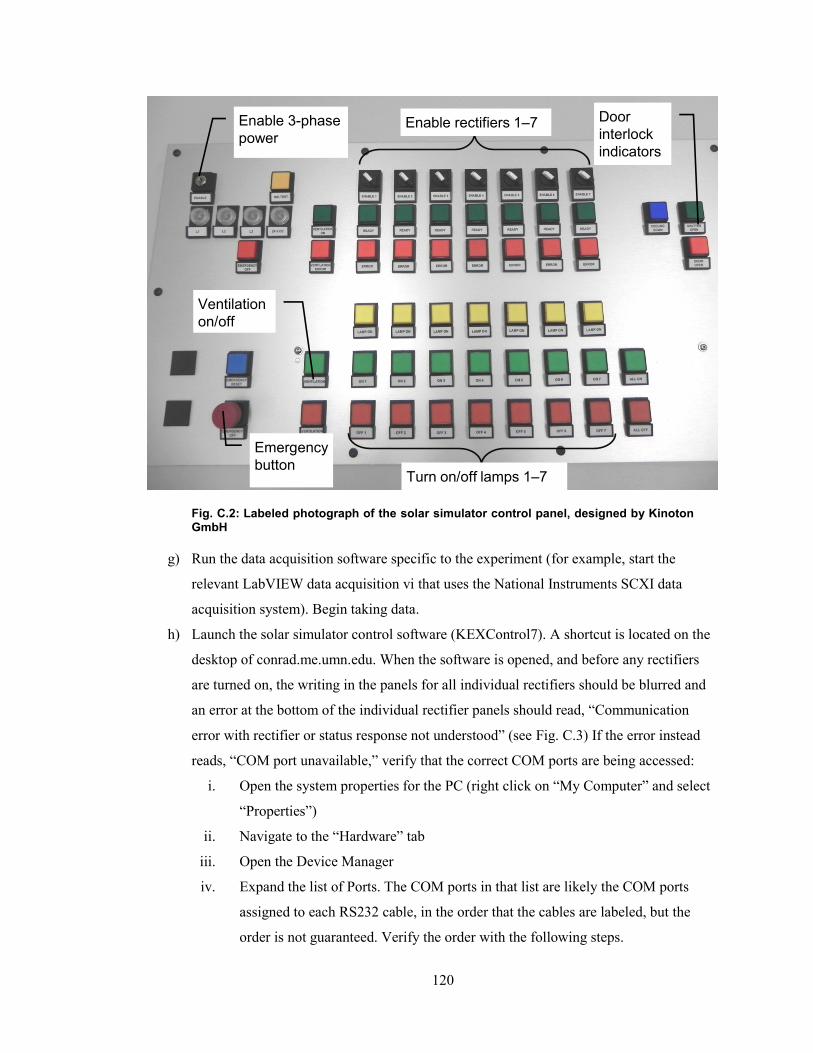
120

Fig. C.2: Labeled photograph of the solar simulator control panel, designed by Kinoton GmbH

g) Run the data acquisition software specific to the experiment (for example, start the

relevant LabVIEW data acquisition vi that uses the National Instruments SCXI data

acquisition system). Begin taking data.

h) Launch the solar simulator control software (KEXControl7). A shortcut is located on the

desktop of conrad.me.umn.edu. When the software is opened, and before any rectifiers

are turned on, the writing in the panels for all individual rectifiers should be blurred and

an error at the bottom of the individual rectifier panels should read, “Communication

error with rectifier or status response not understood” (see Fig. C.3) If the error instead

reads, “COM port unavailable,” verify that the correct COM ports are being accessed:

i. Open the system properties for the PC (right click on “My Computer” and select

“Properties”)

ii. Navigate to the “Hardware” tab

iii. Open the Device Manager

iv. Expand the list of Ports. The COM ports in that list are likely the COM ports

assigned to each RS232 cable, in the order that the cables are labeled, but the

order is not guaranteed. Verify the order with the following steps.

Turn on/off lamps 1–7

Enable rectifiers 1–7 Door

interlock

indicators

Enable 3-phase

power

Emergency

button

Ventilation

on/off

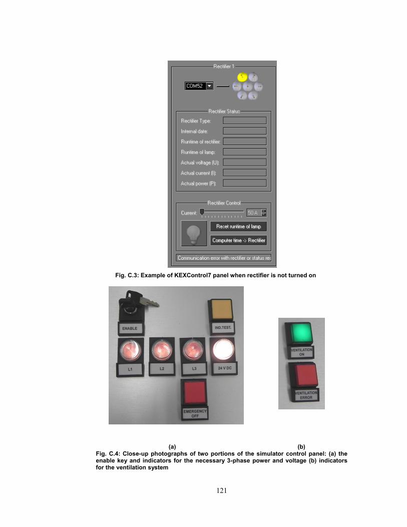
121

Fig. C.3: Example of KEXControl7 panel when rectifier is not turned on

(a) (b) Fig. C.4: Close-up photographs of two portions of the simulator control panel: (a) the enable key and indicators for the necessary 3-phase power and voltage (b) indicators for the ventilation system

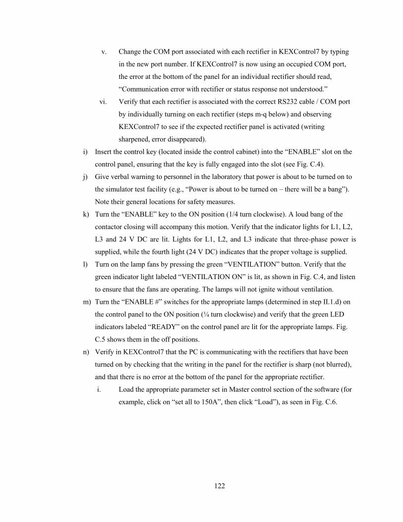
122

v. Change the COM port associated with each rectifier in KEXControl7 by typing

in the new port number. If KEXControl7 is now using an occupied COM port,

the error at the bottom of the panel for an individual rectifier should read,

“Communication error with rectifier or status response not understood.”

vi. Verify that each rectifier is associated with the correct RS232 cable / COM port

by individually turning on each rectifier (steps m-q below) and observing

KEXControl7 to see if the expected rectifier panel is activated (writing

sharpened, error disappeared).

i) Insert the control key (located inside the control cabinet) into the “ENABLE” slot on the

control panel, ensuring that the key is fully engaged into the slot (see Fig. C.4).

j) Give verbal warning to personnel in the laboratory that power is about to be turned on to

the simulator test facility (e.g., “Power is about to be turned on – there will be a bang”).

Note their general locations for safety measures.

k) Turn the “ENABLE” key to the ON position (1/4 turn clockwise). A loud bang of the

contactor closing will accompany this motion. Verify that the indicator lights for L1, L2,

L3 and 24 V DC are lit. Lights for L1, L2, and L3 indicate that three-phase power is

supplied, while the fourth light (24 V DC) indicates that the proper voltage is supplied.

l) Turn on the lamp fans by pressing the green “VENTILATION” button. Verify that the

green indicator light labeled “VENTILATION ON” is lit, as shown in Fig. C.4, and listen

to ensure that the fans are operating. The lamps will not ignite without ventilation.

m) Turn the “ENABLE #” switches for the appropriate lamps (determined in step II.1.d) on

the control panel to the ON position (¼ turn clockwise) and verify that the green LED

indicators labeled “READY” on the control panel are lit for the appropriate lamps. Fig.

C.5 shows them in the off positions.

n) Verify in KEXControl7 that the PC is communicating with the rectifiers that have been

turned on by checking that the writing in the panel for the rectifier is sharp (not blurred),

and that there is no error at the bottom of the panel for the appropriate rectifier.

i. Load the appropriate parameter set in Master control section of the software (for

example, click on “set all to 150A”, then click “Load”), as seen in Fig. C.6.

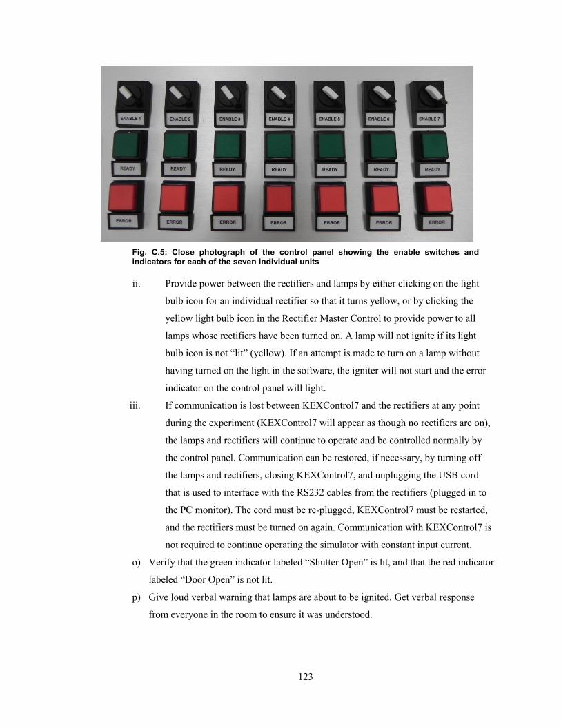
123

Fig. C.5: Close photograph of the control panel showing the enable switches and indicators for each of the seven individual units

ii. Provide power between the rectifiers and lamps by either clicking on the light

bulb icon for an individual rectifier so that it turns yellow, or by clicking the

yellow light bulb icon in the Rectifier Master Control to provide power to all

lamps whose rectifiers have been turned on. A lamp will not ignite if its light

bulb icon is not “lit” (yellow). If an attempt is made to turn on a lamp without

having turned on the light in the software, the igniter will not start and the error

indicator on the control panel will light.

iii. If communication is lost between KEXControl7 and the rectifiers at any point

during the experiment (KEXControl7 will appear as though no rectifiers are on),

the lamps and rectifiers will continue to operate and be controlled normally by

the control panel. Communication can be restored, if necessary, by turning off

the lamps and rectifiers, closing KEXControl7, and unplugging the USB cord

that is used to interface with the RS232 cables from the rectifiers (plugged in to

the PC monitor). The cord must be re-plugged, KEXControl7 must be restarted,

and the rectifiers must be turned on again. Communication with KEXControl7 is

not required to continue operating the simulator with constant input current.

o) Verify that the green indicator labeled “Shutter Open” is lit, and that the red indicator

labeled “Door Open” is not lit.

p) Give loud verbal warning that lamps are about to be ignited. Get verbal response

from everyone in the room to ensure it was understood.

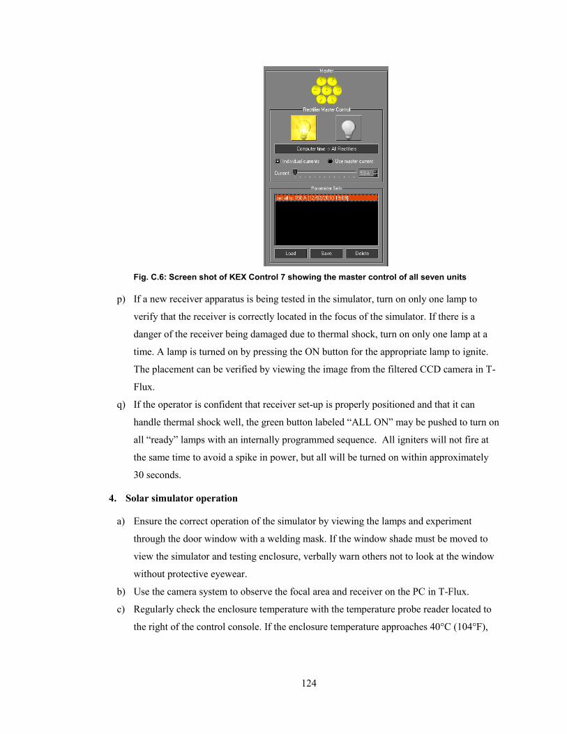
124

Fig. C.6: Screen shot of KEX Control 7 showing the master control of all seven units

p) If a new receiver apparatus is being tested in the simulator, turn on only one lamp to

verify that the receiver is correctly located in the focus of the simulator. If there is a

danger of the receiver being damaged due to thermal shock, turn on only one lamp at a

time. A lamp is turned on by pressing the ON button for the appropriate lamp to ignite.

The placement can be verified by viewing the image from the filtered CCD camera in T-

Flux.

q) If the operator is confident that receiver set-up is properly positioned and that it can

handle thermal shock well, the green button labeled “ALL ON” may be pushed to turn on

all “ready” lamps with an internally programmed sequence. All igniters will not fire at

the same time to avoid a spike in power, but all will be turned on within approximately

30 seconds.

4. Solar simulator operation

a) Ensure the correct operation of the simulator by viewing the lamps and experiment

through the door window with a welding mask. If the window shade must be moved to

view the simulator and testing enclosure, verbally warn others not to look at the window

without protective eyewear.

b) Use the camera system to observe the focal area and receiver on the PC in T-Flux.

c) Regularly check the enclosure temperature with the temperature probe reader located to

the right of the control console. If the enclosure temperature approaches 40°C (104°F),

125

turn off one or more lamps to lower the power or end the experiment. If the enclosure

reaches 40°C, the lamps will shut off for their own protection.

d) Regularly monitor the control panel for red “error” indicator lights. Closely monitor the

relevant experimental controls and data acquisition applications.

5. Solar simulator shutdown

a) Press the red “ALL OFF” button to switch off all of the lamps with an internally

programmed sequence, or turn off individual lamps by pressing the red “OFF #” button

for the specified lamp.

b) Once the lamps are off, press the gray light bulb button in the Rectifier Master Control

panel of the KEXControl7 software to disconnect power between all lamps and rectifiers.

c) Once the lamp has been turned off, turn the rectifier “ENABLE #” switches on the

control panel ¼ turn counterclockwise to the OFF position (11 o’clock) and ensure that

the green “READY” indicator lights are off. In the KEXControl7 software, the writing in

the panels for the rectifiers that have been turned off should blur, and an error at the

bottom of the panel should read, “Communication error with rectifier or status response

not understood.”

d) Turn off the fans by pressing the red “VENTILATION OFF” button. The fans will stay

on for 10 minutes after they have been switched off to ensure proper lamp cooling.

During this time, the blue “COOLING DOWN” indicator is lit. Do not turn off the power

to the control panel (by the enable key) during the 10 minutes of cool-down.

e) After the fans have timed out (turned off after 10 minutes), turn off the power to the

facility by turning the main “ENABLE” key ¼ turn counterclockwise. A loud sound of

the contactors opening accompanies this motion.

f) Close the internal overhead door (shutter). WARNING: Do not enter the testing

enclosure while the shutter is open and when the lamps are hot. If it is absolutely

necessary to go near the lamps while they are hot, cover all exposed skin with clothing,

gloves, and a face shield.

g) Open the man door, and return the red internal safety switch to the off position (down,

unlit).

5. Closing checks

a) Once the internal shutter is closed, the external overhead door may be opened if needed.

Be cautious around the hot experimental apparatus.

b) Remove the warning sign from the door to ME 1134.

126

c) In the T-Flux software, turn off live view, disable the camera, and quit T-Flux.

d) Exit KEXControl7

e) Continue monitoring the temperature of the outlet stream of cooling water from the

receiver setup. Once it has reached a sufficiently cool temperature (approximately

ambient), turn off the cooling water and drain excess water into a bucket for disposal in

the sink drain.

f) Switch off the gas, exhaust and vacuum valves if relevant.

g) Stop the run of the experimental LabVIEW vi, save experimental data, and close

LabVIEW software.

h) Turn off the National Instruments SCXI data acquisition hardware.

i) Switch off the PC system.

j) Collect and store the UV protective equipment.

k) The receiver setup (target, cavity, or other receiving device/material) may be removed

from the focal area if applicable

127

Appendix D.

Heat Flux Gage Thermal Analysis

The following section demonstrates the method used to calculate the incident irradiation by

the heat transfer model from the following parameters: measured gage temperature Tg, average

target temperature tarT that is the average of the four target temperatures shown (Ttar,1, Ttar,2, Ttar,3,

and Ttar,4) cooling water mass flow rate m , and the change in temperature between outlet and

inlet cooling water streams T, as discussed in Chapter 5. The sample calculation uses values

measured when all seven units were operating, which are shown in Table D.1. These values were

averaged from 75 points (250 seconds), taken after both the simulator lamps and the flux

measurement equipment reached steady state. All data used in the heat flux gage calibration were

averaged from at least 40 points. Further constants required for the calculations include the total

hemispherical absorptivity of the heat flux gage (as calculated by Eq. (5.8) using the xenon

emission spectrum), the thermal conductivity of the aluminum target k, the contact resistance

between the gage and the target ct,R , the diameter of the heat flux gage d1, and the diameter of

the circle containing the locations of the four target thermocouples d2. The values of the constants

are shown in Table D.2.

The Nth order uncertainty in each measurand is determined by using the root-sum-square

method, as presented by Kline & McClintock [78], to combine the first order uncertainty with the

instrument precision. The first order uncertainty (or precision) is calculated using the student-t

distribution for a 95% confidence interval. The uncertainty values of the resulting energy rates

and radiative fluxes were estimated using the sequential perturbation method. In this method,

each measurand is individually perturbed by its Nth order uncertainty—first by adding the

uncertainty (“up” perturbation) and then by subtracting it (“down” perturbation) from the nominal

value—and the perturbed measurand is propagated through all parts of the calculation to arrive at

a perturbed result. The difference between each perturbed and the nominal result is stored and

averaged for each set of “up” and “down” perturbations. The measurand is returned to its nominal

value and the process begins again for the next variable. Once all measurands have been

perturbed, the set of averaged differences in the resultant values is combined using the root-sum-

square method to arrive at the total uncertainty in the result. Further details of this method are

discussed in Figliola & Beasley [72].

For the data presented in Table D.1, the following values were calculated: the energy rate

absorbed by the water was Tcm p =2164±13 W and the energy conducted between the gage and

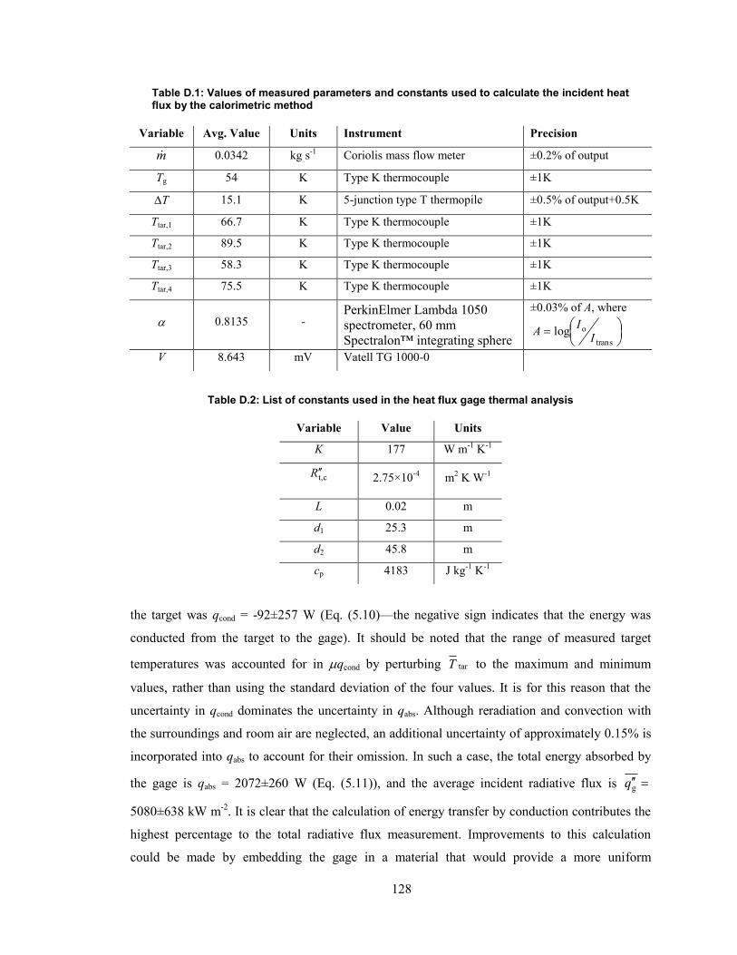
128

Table D.1: Values of measured parameters and constants used to calculate the incident heat flux by the calorimetric method

Variable Avg. Value Units Instrument Precision

m 0.0342 kg s-1

Coriolis mass flow meter ±0.2% of output

Tg 54 K Type K thermocouple ±1K

T 15.1 K 5-junction type T thermopile ±0.5% of output+0.5K

Ttar,1 66.7 K Type K thermocouple ±1K




0.8135 - PerkinElmer Lambda 1050

spectrometer, 60 mm

Spectralon™ integrating sphere

±0.03% of A, where

trans

ologI

IA

V 8.643 mV Vatell TG 1000-0

Table D.2: List of constants used in the heat flux gage thermal analysis

Variable Value Units

K 177 W m-1

K-1

ct,R 2.75×10-4

m2 K W

-1

L 0.02 m

d1 25.3 m

d2 45.8 m

cp 4183 J kg-1

K-1

the target was qcond = -92±257 W (Eq. (5.10)—the negative sign indicates that the energy was

conducted from the target to the gage). It should be noted that the range of measured target

temperatures was accounted for in qcond by perturbing tarT to the maximum and minimum

values, rather than using the standard deviation of the four values. It is for this reason that the

uncertainty in qcond dominates the uncertainty in qabs. Although reradiation and convection with

the surroundings and room air are neglected, an additional uncertainty of approximately 0.15% is

incorporated into qabs to account for their omission. In such a case, the total energy absorbed by

the gage is qabs = 2072±260 W (Eq. (5.11)), and the average incident radiative flux is gq

5080±638 kW m-2

. It is clear that the calculation of energy transfer by conduction contributes the

highest percentage to the total radiative flux measurement. Improvements to this calculation

could be made by embedding the gage in a material that would provide a more uniform

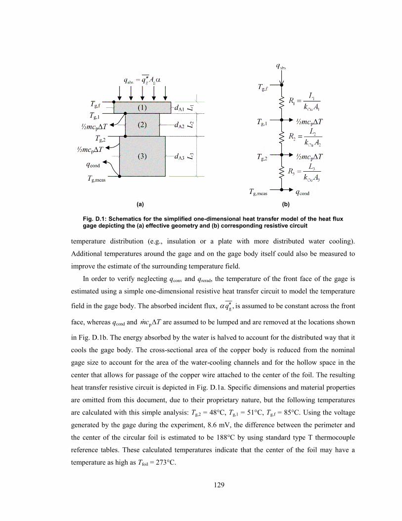
129

(a) (b)

Fig. D.1: Schematics for the simplified one-dimensional heat transfer model of the heat flux gage depicting the (a) effective geometry and (b) corresponding resistive circuit

temperature distribution (e.g., insulation or a plate with more distributed water cooling).

Additional temperatures around the gage and on the gage body itself could also be measured to

improve the estimate of the surrounding temperature field.

In order to verify neglecting qconv and qrerad, the temperature of the front face of the gage is

estimated using a simple one-dimensional resistive heat transfer circuit to model the temperature

field in the gage body. The absorbed incident flux, ,gq is assumed to be constant across the front

face, whereas qcond and Tcm p are assumed to be lumped and are removed at the locations shown

in Fig. D.1b. The energy absorbed by the water is halved to account for the distributed way that it

cools the gage body. The cross-sectional area of the copper body is reduced from the nominal

gage size to account for the area of the water-cooling channels and for the hollow space in the

center that allows for passage of the copper wire attached to the center of the foil. The resulting

heat transfer resistive circuit is depicted in Fig. D.1a. Specific dimensions and material properties

are omitted from this document, due to their proprietary nature, but the following temperatures

are calculated with this simple analysis: Tg,2 = 48°C, Tg,1 = 51°C, Tg,f = 85°C. Using the voltage

generated by the gage during the experiment, 8.6 mV, the difference between the perimeter and

the center of the circular foil is estimated to be 188°C by using standard type T thermocouple

reference tables. These calculated temperatures indicate that the center of the foil may have a

temperature as high as Tfoil = 273°C.

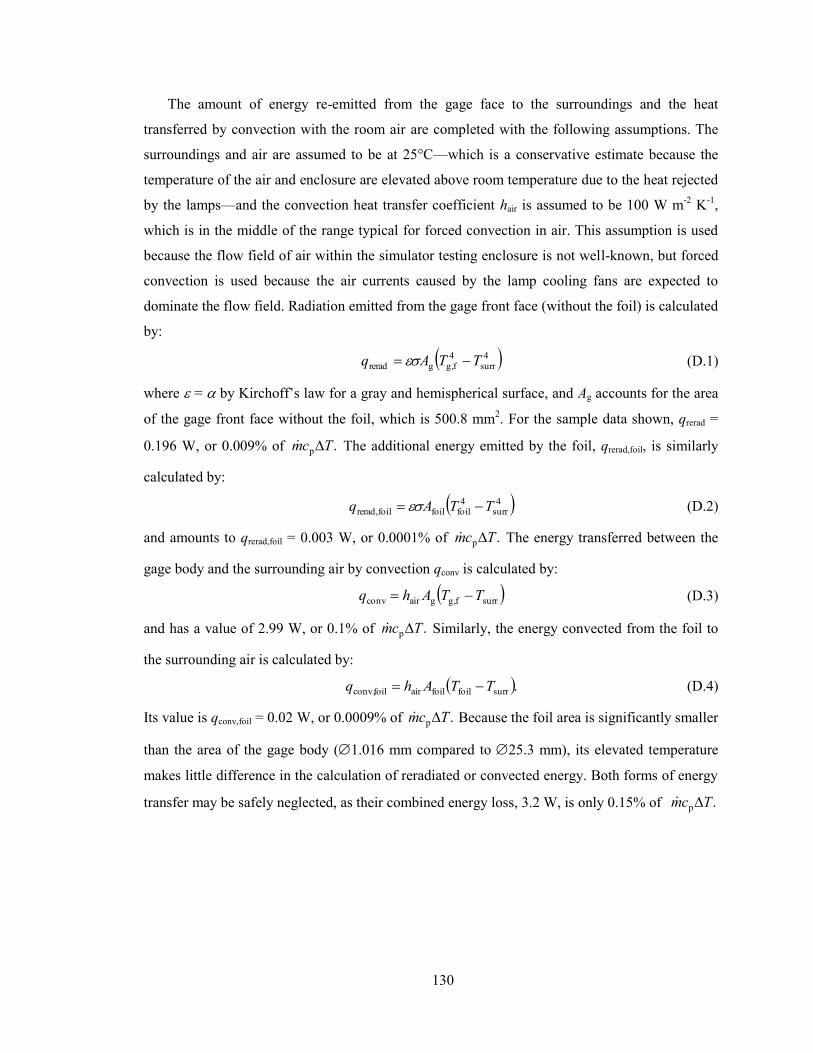
130

The amount of energy re-emitted from the gage face to the surroundings and the heat

transferred by convection with the room air are completed with the following assumptions. The

surroundings and air are assumed to be at 25°C—which is a conservative estimate because the

temperature of the air and enclosure are elevated above room temperature due to the heat rejected

by the lamps—and the convection heat transfer coefficient hair is assumed to be 100 W m-2

K-1

,

which is in the middle of the range typical for forced convection in air. This assumption is used

because the flow field of air within the simulator testing enclosure is not well-known, but forced

convection is used because the air currents caused by the lamp cooling fans are expected to

dominate the flow field. Radiation emitted from the gage front face (without the foil) is calculated

by:

4surr

4fg,grerad TTAq (D.1)

where = by Kirchoff’s law for a gray and hemispherical surface, and Ag accounts for the area

of the gage front face without the foil, which is 500.8 mm2. For the sample data shown, qrerad =

0.196 W, or 0.009% of .p Tcm The additional energy emitted by the foil, qrerad,foil, is similarly

calculated by:

4surr

4foilfoilfoilrerad, TTAq (D.2)

and amounts to qrerad,foil = 0.003 W, or 0.0001% of .p Tcm The energy transferred between the

gage body and the surrounding air by convection qconv is calculated by:

surrfg,gairconv TTAhq (D.3)

and has a value of 2.99 W, or 0.1% of .p Tcm Similarly, the energy convected from the foil to

the surrounding air is calculated by:

.surrfoilfoilairfoilconv, TTAhq (D.4)

Its value is qconv,foil = 0.02 W, or 0.0009% of .p Tcm Because the foil area is significantly smaller

than the area of the gage body (1.016 mm compared to 25.3 mm), its elevated temperature

makes little difference in the calculation of reradiated or convected energy. Both forms of energy

transfer may be safely neglected, as their combined energy loss, 3.2 W, is only 0.15% of .p Tcm

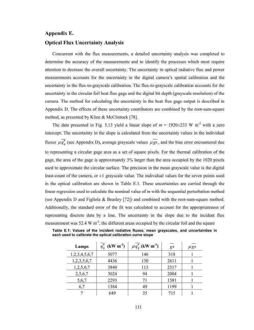
131

Appendix E.

Optical Flux Uncertainty Analysis

Concurrent with the flux measurements, a detailed uncertainty analysis was completed to

determine the accuracy of the measurements and to identify the processes which most require

attention to decrease the overall uncertainty. The uncertainty in optical radiative flux and power

measurements accounts for the uncertainty in the digital camera’s spatial calibration and the

uncertainty in the flux-to-grayscale calibration. The flux-to-grayscale calibration accounts for the

uncertainty in the circular foil heat flux gage and the digital bit depth (grayscale resolution) of the

camera. The method for calculating the uncertainty in the heat flux gage output is described in

Appendix D. The effects of these uncertainty contributors are combined by the root-sum-square

method, as presented by Kline & McClintock [78].

The data presented in Fig. 5.13 yield a linear slope of m = 1920±233 W m-2

with a zero

intercept. The uncertainty in the slope is calculated from the uncertainty values in the individual

fluxes gq (see Appendix D), average grayscale values gs , and the bias error encountered due

to representing a circular gage area as a set of square pixels. For the thermal calibration of the

gage, the area of the gage is approximately 3% larger than the area occupied by the 1020 pixels

used to approximate the circular surface. The precision in the mean grayscale value is the digital

least-count of the camera, or ±1 grayscale value. The individual values for the seven points used

in the optical calibration are shown in Table E.1. These uncertainties are carried through the

linear regression used to calculate the nominal value of m with the sequential perturbation method

(see Appendix D and Figliola & Beasley [72]) and combined with the root-sum-square method.

Additionally, the standard error of the fit was calculated to account for the appropriateness of

representing discrete data by a line. The uncertainty in the slope due to the incident flux

measurement was 52.4 W m-2

, the different areas occupied by the circular foil and the square

Table E.1: Values of the incident radiative fluxes, mean grayscales, and uncertainties in each used to calibrate the optical calibration curve slope

Lamps gq (kW m-2

) gq (kW m-2

) gs gs

1,2,3,4,5,6,7 5077 146 318 1

1,2,3,5,6,7 4436 130 2611 1

1,2,5,6,7 3840 113 2317 1

2,5,6,7 3024 94 2004 1

5,6,7 2293 71 1581 1

6,7 1384 49 1199 1

7 649 35 715 1

132

pixels contributed 59.4 W m-2

, the uncertainty in the slope due to the grayscale resolution was

only 2×10-12

W m-2

, and the standard error of the fit contributed 23.8 W m-2

. If necessary, the

largest contributor, the uncertainty due to the camera’s spatial resolution, could be improved by

selecting a camera with a higher spatial resolution.

Further uncertainty values incorporated into the calibration constant Kf by Eq. (5.14) include

the precision of the spatial calibration. The printer used to generate the grid of dots used in the

spatial calibration has a resolution of 600 dpi (dots per inch), which corresponds to a spatial

resolution of 0.042 mm. This uncertainty was perturbed through the calculation of Kf to

contribute 4.4×10-7

W s, whereas the contribution from the slope was 2.4 ×10-6

W s.

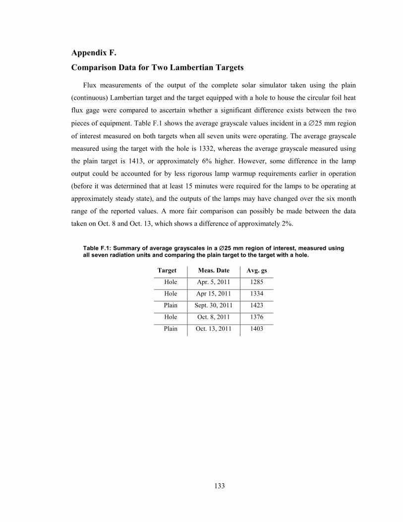
133

Appendix F.

Comparison Data for Two Lambertian Targets

Flux measurements of the output of the complete solar simulator taken using the plain

(continuous) Lambertian target and the target equipped with a hole to house the circular foil heat

flux gage were compared to ascertain whether a significant difference exists between the two

pieces of equipment. Table F.1 shows the average grayscale values incident in a 25 mm region

of interest measured on both targets when all seven units were operating. The average grayscale

measured using the target with the hole is 1332, whereas the average grayscale measured using

the plain target is 1413, or approximately 6% higher. However, some difference in the lamp

output could be accounted for by less rigorous lamp warmup requirements earlier in operation

(before it was determined that at least 15 minutes were required for the lamps to be operating at

approximately steady state), and the outputs of the lamps may have changed over the six month

range of the reported values. A more fair comparison can possibly be made between the data

taken on Oct. 8 and Oct. 13, which shows a difference of approximately 2%.

Table F.1: Summary of average grayscales in a 25 mm region of interest, measured using all seven radiation units and comparing the plain target to the target with a hole.

Target Meas. Date Avg. gs

Hole Apr. 5, 2011 1285

Hole Apr 15, 2011 1334

Plain Sept. 30, 2011 1423

Hole Oct. 8, 2011 1376

Plain Oct. 13, 2011 1403

Design and Characterization of a Concentrating Solar Simulator

Documents

Transcript of Design and Characterization of a Concentrating Solar Simulator