Outline of the Earth Simulator Project

i

CONTENTS

Outline of the Earth Simulator Project1. Mission and Basic Principles of the Earth Simulator ························································································································································· 12. Earth Simulator Research Project ·································································································································································································· 13. Collaboration Projects ·························································································································································································································· 44. System Configuration of the Earth Simulator ········································································································································································· 4

Earth Simulator Research Projects

Chapter 1 Earth Science

Understanding Roles of Oceanic Fine Structures in Climate and Its Variability II ····························································································· 11Wataru Ohfuchi Earth Simulator Center, Japan Agency for Marine-Earth Science and Technology海洋微細構造が生み出す気候形成・変動メカニズムの解明海洋研究開発機構　地球シミュレータセンター　　大淵　済

Adaptation Oriented Simulations for Climate Variability ·················································································································································· 17Keiko Takahashi Earth Simulator Center, Japan Agency for Marine-Earth Science and Technology気候変動に適応可能な環境探索のためのマルチスケールシミュレーション海洋研究開発機構　地球シミュレータセンター　　高橋　桂子

Development of a High-Resolution Coupled Climate Model for Global Warming Studies ··········································································· 23Akira Noda Research Institute for Global Change, Japan Agency for Marine-Earth Science and Technology地球温暖化予測研究のための高精度気候モデルの開発研究海洋研究開発機構　地球環境変動領域　　野田　彰

Simulations of Atmospheric General Circulations of Earth-like Planets by AFES ····························································································· 29Yoshi-Yuki Hayashi Department of Earth and Planetary Sciences, Kobe UniversityAFESを用いた地球型惑星の大気大循環シミュレーション神戸大学大学院　理学研究科　　林　祥介

Study on the Diagnostics and Projection of Ecosystem Change Associated with Global Change ······························································ 35Michio J. Kishi Research Institute for Global Change, Japan Agency for Marine-Earth Science and Technology地球環境変化に伴う生態系変動の診断と予測に関する研究海洋研究開発機構　地球環境変動領域　　岸　道郎

Three-Dimensional Nonsteady Coupled Analysis of Thermal Environment and Energy Systems in Urban Area ···························· 39Yasunobu Ashie National Institute for Land and Infrastructure Management地域熱環境と空調負荷の 3次元非定常連成解析国土技術政策総合研究所　　足永　靖信

Study of Cloud and Precipitation Processes using a Global Cloud Resolving Model ························································································ 43Masaki Satoh Research Institute for Global Change, Japan Agency for Marine-Earth Science and Technology

Atmosphere and Ocean Research Institute, The University of Tokyo全球雲解像モデルを用いた雲降水プロセス研究海洋研究開発機構　地球環境変動領域　　佐藤　正樹　　東京大学　大気海洋研究所

ii

Process Studies and Seasonal Prediction Experiment using Coupled General Circulation Model ····························································· 51Yukio Masumoto Research Institute for Global Change, Japan Agency for Marine-Earth Science and Technology大気海洋結合モデルを用いたプロセス研究と季節予測実験海洋研究開発機構　地球環境変動領域　　升本　順夫

Simulation and Verification of Tropical Deep Convective Clouds using Eddy-Permitting Regional Atmospheric Models ······················································································································································· 55Kozo Nakamura Research Institute for Global Change, Japan Agency for Marine-Earth Science and Technology渦解像可能な領域大気モデルを用いた深い対流のシミュレーションとその検証海洋研究開発機構　地球環境変動領域　　中村　晃三

Estimation of the Variation of Atmospheric Composition and Its Effect on the Climate Change by using a Chemical Transport Model··························································································································································································· 59Masayuki Takigawa Research Institute for Global Change, Japan Agency for Marine-Earth Science and Technology化学輸送モデルによる大気組成変動と気候影響の研究海洋研究開発機構　地球環境変動領域　　滝川　雅之

Improved Estimates of the Dynamical Ocean State by using a 4D-VAR Adjoint Method ············································································· 63Shuhei Masuda Research Institute for Global Change, Japan Agency for Marine-Earth Science and Technology四次元変分法海洋データ同化システムを用いた海洋環境再現実験海洋研究開発機構　地球環境変動領域　　増田　周平

Realistic High-Frequency Global Barotropic Ocean Modeling Driven by Synoptic Atmospheric Disturbances ······························· 67Ryota Hino Research Center for Prediction of Earthquakes and Volcanic Eruptions,

Graduate School of Science, Tohoku University総観規模の大気擾乱に伴う現実的な短周期全球順圧海洋モデリング東北大学大学院　理学研究科　地震・噴火予知研究観測センター　　日野　亮太

Global Elastic Response Simulation ······························································································································································································· 75Seiji Tsuboi Institute for Research on Earth Evolution / Data Research Center for Marine-Earth Sciences,

Japan Agency for Marine-Earth Science and Technology全地球弾性応答シミュレーション海洋研究開発機構　地球内部ダイナミクス領域 /地球情報研究センター　　坪井　誠司

Simulation Study on the Dynamics of the Mantle and Core in Earth-like Conditions ······················································································· 81Yozo Hamano Institute for Research on Earth Evolution, Japan Agency for Marine-Earth Science and Technology実地球環境でのマントル・コア活動の数値シミュレーション海洋研究開発機構　地球内部ダイナミクス領域　　浜野　洋三

Development of a Predictive Simulation System for Crustal Activities in and around Japan - VIII ························································· 89Chihiro Hashimoto Graduate School of Environmental Studies, Nagoya University日本列島域の地殻活動予測シミュレーション・システムの開発 - Ⅷ名古屋大学大学院　環境学研究科　　橋本　千尋

Tsunami Simulation for the Great 1707 Hoei, Japan, Earthquake using the Earth Simulator ······································································· 95Takashi Furumura Center for Integrated Disaster Information Research, Interfaculty Initiative in Information Studies,

The University of Tokyo / Earthquake Research Institute, The University of Tokyo地球シミュレータによる 1707 年宝永地震の津波シミュレーション東京大学大学院　情報学環　総合防災情報研究センター　　古村　孝志東京大学　地震研究所

iii

Development of Advanced Simulation Methods for Solid Earth Simulations····································································································· 103Akira Kageyama Graduate School of System Informatics, Kobe University先端的固体地球科学シミュレーションコードの開発神戸大学大学院　システム情報学研究科　　陰山　聡

3-D Numerical Simulations of Volcanic Eruption Column Collapse ······················································································································· 107Takehiro Koyaguchi Earthquake Research Institute, The University of Tokyo3次元数値シミュレーションによる噴煙柱崩壊条件の解析東京大学　地震研究所　　小屋口　剛博

Space and Earth System Modeling ······························································································································································································· 113Kanya Kusano Institute for Research on Earth Evolution, Japan Agency for Marine-Earth Science and Technology宇宙・地球表層・地球内部の相関モデリング海洋研究開発機構　地球内部ダイナミクス領域　　草野　完也

Chapter 2 Epoch-Making Simulation

Development of General Purpose Numerical Software Infrastructure for Large Scale Scientific Computing ·································· 119Akira Nishida Research Institute for Information Technology, Kyushu University大規模科学計算向け汎用数値ソフトウェア基盤の開発九州大学　情報基盤研究開発センター　　西田　晃

Large Scale Simulations for Carbon Nanotubes ··································································································································································· 125Syogo Tejima Research Organization for Information Science & Technologyカーボンナノチューブの特性に関する大規模シミュレーション高度情報科学技術研究機構　　手島　正吾

Development of the Next-generation Computational Fracture Mechanics Simulator for Constructing Safe and Sustainable Society ······································································································································································ 131Ryuji Shioya Faculty of Information Sciences and Arts, Toyo University安全・安心な持続可能社会のための次世代計算破壊力学シミュレータの開発東洋大学　総合情報学部　　塩谷　隆二

Large-scale Simulation for a Terahertz Resonance Superconductor Device ········································································································ 135Mikio Iizuka Research Organization for Information Science and Technologyテラヘルツ発振超伝導素子に関する大規模シミュレーション高度情報科学技術研究機構　　飯塚　幹夫

Direct Numerical Simulations of Fundamental Turbulent Flows with the World's Largest Number of Grid-points and Application to Modeling of Engineering Turbulent Flows ···································································································································· 143Yukio Kaneda Graduate School of Engineering, Nagoya University乱流の世界最大規模直接数値計算とモデリングによる応用計算名古屋大学大学院　工学研究科　　金田　行雄

A Large-scale Genomics and Proteomics Analyses Conducted by the Earth Simulator ················································································ 149Toshimichi Ikemura Nagahama Institute of Bio-Science and TechnologyES を用いた大規模ゲノム・プロテオミクス解析：多様な環境由来の大量メタゲノム配列から、重要な代謝経路を保持する有用ゲノム資源を探索する新規戦略長浜バイオ大学　バイオサイエンス学部　　池村　淑道

iv

First-principles Calculation on Peierls Potential of an Isolated Screw Dislocation in BCC Iron ······························································ 157Hideo Kaburaki Japan Atomic Energy Agency第一原理計算による BCC鉄中らせん転位のパイエルスポテンシャルの計算日本原子力研究開発機構蕪木　英雄

Development of a Fluid Simulation Approach by Massively Parallel Bit-wise Operations with a New Viscosity Control Method ······················································································································································································· 161Hiroshi Matsuoka Research Institute of Electrical Communication, Tohoku University新粘性制御法による超並列ビット演算流体シミュレーション手法の開発東北大学　電気通信研究所　　松岡　浩

RSA Decryption using Earth Simulator ····················································································································································································· 167Hidehiko Hasegawa Graduate School of Library, Information and Media Studies, University of Tsukuba地球シミュレータを用いた RSA暗号解読処理筑波大学大学院　図書館情報メディア研究科　　長谷川　秀彦

Development of Sophisticated Simulation Analysis Method of Actual Reinforced Concrete Building by Shaking Table Test-I ······················································································································································································································ 173Yoshiyuki Kasai Department of Urban Environment and Information Sciences, Graduate School,

Maebashi Institute of Technology実大鉄筋コンクリート造建物の振動台実験の精密・詳細シミュレーション解析システムの開発　その 1

前橋工科大学大学院　工学研究科　環境・情報工学専攻　　河西　良幸　

Numerical Simulations of Droplet Splashing ········································································································································································· 181Feng Xiao Interdisciplinary Graduate School of Science and Engineering, Tokyo Institute of Technology水滴衝突（スプラッシュ）の数値的研究東京工業大学大学院　総合理工学研究科　　肖　鋒　

Large-Scale Electronic-State Calculations of Influenza Viral Proteins with Fragment Molecular Orbital Method and Applications to Mutation Prediction ······················································································ 187Shigenori Tanaka Graduate School of System Informatics, Kobe Universityフラグメント分子軌道法によるインフルエンザウイルスタンパク質の大規模電子状態計算と変異予測への応用神戸大学大学院　システム情報学研究科　　田中　成典

Chapter 3 Visualization

Studies of Large-Scale Data Visualization: EXTRAWING and Visual Data Mining ····················································································· 195Fumiaki Araki Earth Simulator Center, Japan Agency for Marine-Earth Science and Technology大規模データ可視化研究 : EXTRAWINGとビジュアルデータマイニング海洋研究開発機構　地球シミュレータセンター　　荒木　文明

1

Outline of the Earth Simulator Project

1. Mission and Basic Principles of the Earth SimulatorThe Earth Simulator was developed for the following aims. The first aim is to ensure a bright future for human beings by

accurately predicting variable global environment. The second is to contribute to the development of science and technology in the 21st century. Based on these aims, the principles listed below are established for the projects of the Earth Simulator.

1) Each project should be open to researches in each research field and to the public, rather than it is confined within the limited research society.

2) In principle, the research achievements obtained by using the Earth Simulator should be promptly published and returned to the public.

3) Each project should be carried out for peaceful purposes only.

2. Earth Simulator Research ProjectThere are two fields of Earth Simulator Research Projects, as follows:• Earth Science• Epoch-making Simulation

The allocation of Earth Simulator resources for each research field in FY2010 was decided to be as shown in following graph.

Public project recruitment for Earth Simulator Research Projects in FY2010 was held in February 2010, and 31 research projects were selected by the Selection Committee.

The Allocation of Resources of the Earth Simulator in FY2010

2

Authorized Projects in FY2010

Earth Science (19 projects)

Title Project leader Affiliation of project leader

1Understanding Roles of Oceanic Fine Structures in Climate and its Variability

Wataru Ofuchi ESC, JAMSTEC

2Simulations of Adaptation-Oriented Strategy for Climate Variability

Keiko Takahashi ESC, JAMSTEC

3Development of a High-quality Climate Model for Global Warming Projection Study

Akira Noda RIGC, JAMSTEC

4Simulations of Atmospheric General Circulations of Earth-like Planets by AFES

Yoshiyuki Hayashi Graduate School of Science, Kobe University

5Study on the Diagnostics and Projection of Ecosystem Change Associated with Global Change

Michio Kishi RIGC, JAMSTEC

6Development of a Numerical Model of Urban Heat Island

Yasunobu AshieNational Institute for Land and Infrastructure Management

7Study of Cloud and Precipitation Processes using a Global Cloud-system Resolving Model

Masaki SatoRIGC, JAMSTEC/Atmosphere and Ocean Research Institute, The University of Tokyo

8Study on Predictability of Climate Variations and Their Mechanisms

Yukio Masumoto RIGC, JAMSTEC

9Simulation and Verification of Tropical Deep Convective Clouds using Eddy-permitting Regional Atmospheric Models

Kozo Nakamura RIGC, JAMSTEC

10Atmospheric Composition Change and its Climate Effect Studies by a Chemical Transport Model

Masayuki Takigawa RIGC, JAMSTEC

11

Ocean State Estimation for the Recent Decade and Adjoint Sensitivity Analysis for the Optimal Observing System, by using a 4D-VAR Ocean Data Assimilation Model

Shuhei Masuda RIGC, JAMSTEC

12High-frequency Global Ocean Modeling with the 1-km Spatial Resolution

Ryota HinoResearch Center for Prediction of Earthquakes and Volcanic Eruptions, Graduate School of Science, Tohoku University

13 Global Elastic Response Simulation Seiji Tsuboi IFREE/DrC, JAMSTEC

14Simulation Study on the Dynamics of the Mantle and Core in Earth-like Conditions

Yozo Hamano IFREE, JAMSTEC

15Predictive Simulation for Crustal Activity in and around Japan

Chihiro HashimotoGraduate School of Environmental Studies, Nagoya University

16Numerical Simulation of Seismic Wave Propagation and Strong Ground Motions in 3-D Heterogeneous Media

Takashi Furumura

Center for Integrated Disaster Information Research, Interfaculty Initiative in Information Studies, The University of Tokyo/Earthquake Research Institute, The University of Tokyo

17Development of Advanced Simulation Tools for Solid Earth Sciences

Akira KageyamaGraduate School of System Informatics, Kobe University

18Numerical Simulations of the Dynamics of Volcanic Phenomena

Takehiro KoyaguchiEarthquake Research Institute, The University of Tokyo

19 Space and Earth System Modeling Kanya Kusano IFREE, JAMSTEC

3

Epoch-making Simulation (12 projects)

Title Project leader Affiliation of project leader

20Development of General Purpose Numerical Software Infrastructure for Large Scale Scientific Computing

Akira NishidaResearch Institute for Information Technology, Kyushu University

21Large-scale Simulation on the Properties of Carbon-nanotube

Syogo TejimaResearch Organization for Information Science & Technology

22Development of the Next-generation Computational Fracture Mechanics Simulator for Constructing Safe and Sustainable Society

Ryuji ShioyaFaculty of Information Sciences and Arts, Toyo University

23Large-scale Simulation for a Terahertz Resonance Superconductors Device

Mikio IizukaResearch Organization for Information Science & Technology

24

Direct Numerical Simulations of Fundamental Turbulent Flows with the World's Largest Number of Grid-points and Application to Modeling of Engineering Turbulent Flows

Yukio KanedaGraduate School of Engineering, Nagoya University

25A Large-scale Post-genome Analysis using Self-Organizing Map for All Genome and Protein Sequences

Toshimichi IkemuraNagahama Institute of Bio-Science and Technology

26First Principles Calculation on Hydrogen Diffusion Behavior in Iron Containing a Dislocation and Grain Boundary

Hideo Kaburaki Japan Atomic Energy Agency

27Development of a Fluid Simulation Approach by Massively Parallel Bits-operations with a New Viscosity Control Method

Hiroshi MatsuokaResearch Institute of Electrical Communication, Tohoku University

28 Development of Adaptive High Accuracy Libraries Hidehiko HasegawaGraduate School of Library, Information and Media Studies, University of Tsukuba

29Developments of Sophisticated Simulation Analysis Method of Actual Reinforced Concrete Building by Shaking Table Test

Yoshiyuki KasaiDepartment of Urban Environment and Information Science, Graduate School, Maebashi Institute of Technology

30 Numerical Studies of Droplet Impacts (Splashes) Feng XiaoInterdisciplinary Graduate School of Science and Engineering, Tokyo Institute of Technology

31Theoretical Study of Drug Resistance Mechanism Based on the Fragment Molecular Orbital Method

Shigenori TanakaGraduate School of System Informatics, Kobe University

JAMSTEC : Japan Agency for Marine-Earth Science and TechnologyIFREE : Institute for Research on Earth EvolutionESC : Earth Simulator CenterRIGC : Research Institute for Global ChangeDrC : Data Research Center for Marine-Earth Sciences

4

3. Collaboration Projects

Collaboration Projects in FY2010

• Institut Français de Recherche pour l’Exploitation de la Mer (IFREMER), Département d’Océanographie Physique et Spatiale, France

• Ernest Orlando Lawrence Berkeley National Laboratory, University of California (LBNL), USA

• Korean Ocean Research & Development Institute (KORDI), Korea

• The National Oceanography Centre, Southampton (NOCS), UK

• The large-scale numerical simulation of the weather/oceanographic phenomena for international maritime transportation : Kobe University

• Research and development for MSSG calculation performance optimization in the next-generation supercomputer system : RIKEN

• Collaborative research on the sophistication of the computational simulation software toward constructing the platform for the leading industrial research and development : Institute of Industrial Science, the University of Tokyo

• Numerical study on rheophysical behavior of viscoelastic fluids and their mechanisms using Digital Ink Laboratory (DIL) System : DNP Fine Chemicals Fukushima Co., Ltd

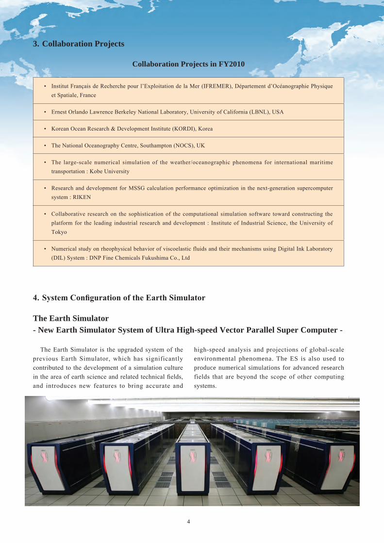
4.SystemConfigurationoftheEarthSimulator

The Earth Simulator - New Earth Simulator System of Ultra High-speed Vector Parallel Super Computer -

The Earth Simulator is the upgraded system of the previous Earth Simulator, which has significantly contributed to the development of a simulation culture in the area of earth science and related technical fields, and introduces new features to bring accurate and

high-speed analysis and projections of global-scale environmental phenomena. The ES is also used to produce numerical simulations for advanced research fields that are beyond the scope of other computing systems.

Earth Simulator Research Projects

Chapter 1

Earth Science

11


1. IntroductionWe have been studying relatively small spatial scale

interaction of the atmosphere and ocean. In this report, we present oceanic variability driven by winds and oceanic internal fluctuation. In chapter 2, deep oceanic zonal jets driven by fine-scale wind stress curls will be presented. Submesoscale oceanic structures simulated by 1/30-degree resolution ocean circulation will be discussed in chapter 3. The Kuroshio Extension Current (KEC) seems to fluctuate by oceanic internal dynamics. Chapter 4 shows a study on KEC variability by a four-member ensemble re-forecast experiment. Oceanic internal solitary-like gravity waves (ISWs) play an important role for vertical mixing. We report ISWs induced by a typhoon in a non-hydrostatic atmosphere–ocean coupled model in chapter 5.

2. Deep oceanic zonal jets driven by fine-scale wind stress curlsOceanic alternating zonal jets at depth have been detected

ubiquitously in observations and OGCMs (Ocean General Circulation Models). It is often expected that the oceanic jets can be generated by purely oceanic processes. Recently, Kessler and Gourdeau [1] (KG) provided another view of the “wind-driven” oceanic zonal jets. Specifically, they analyzed climatological geostrophic currents and satellite-observed wind stress to find bands of meridionally narrow eastward deep currents in the

subtropical South Pacific as consistent with zonal Sverdrup jets forced by meridional fine-scale wind stress curls. Regarding this “wind-driven jet”, however, it is yet to be understood what give rise to such fine-scale wind stress curl structure. The objective of this study is to explore a possible air-sea interaction between the oceanic zonal jets and the fine-scale wind curls using a high-resolution CFES (Coupled GCM for Earth Simulator) [2].

Figure 1a shows the annual mean vertically integrated zonal current in the south pacific from the 23-year CFES integration. The model represents zonally striated structures, including eastward jets embedded in large-scale westward flows in equatorward sides of subtropical gyres. The zonally averaged meridional structure of the zonal jets turns out to be well represented by that of the zonal currents inferred by the Sverdrup relation with the wind stress field taken from the CFES output (Fig. 1b). Thus, there exist in the CFES integration the deep zonal jets driven by the fine-scale wind stress curl as KG's observational analysis. Further analysis shows that the eastward Sverdrup transport peaks in the central South Pacific basin are primarily forced by the meridional gradient of the wind stress curl in the region slightly to the west, which then originates from the meridionally fine-scale wind stress curl itself (Fig. 1d). We found this fine-scale wind stress curl structures are spatially well correlated with the SST laplacian fields (Fig. 1c), suggestive of the wind stress field induced by pressure adjustment in ABL

Understanding Roles of Oceanic Fine Structures in Climate and Its Variability II

Project Representative

Wataru Ohfuchi Earth Simulator Center, Japan Agency for Marine-Earth Science and Technology

Authors

Wataru Ohfuchi*1, Bunmei Taguchi*1, Hideharu Sasaki*1, Masami Nonaka*2, Hidenori Aiki*2 and Mayumi K. Yoshioka*3

*1 Earth Simulator Center, Japan Agency for Marine-Earth Science and Technology

*2 Research Institute for Global Change, Japan Agency for Marine-Earth Science and Technology

*3 Hydrospheric Atmospheric Research Center, Nagoya University

We have been running high-resolution primitive equation and non-hydrostatic, atmosphere, ocean and coupled, global and regional models in order to investigate air-sea interaction where oceanic structures of small spatial scale play important roles. In this report, we present the following four topics. 1) Deep oceanic zonal jets that seem to be driven by fine-scale wind stress curls. 2) Preliminary results from a 1/30-degree resolution North Pacific Ocean circulation simulation. 3) Internal variability of the Kuroshio Extension Current using a four-member ensemble ocean hindcast. 4) Oceanic internal solitary-like gravity waves generated by a typhoon in a coupled atmosphere–ocean non-hydrostatic simulation.

Keywords: Oceanic zonal jets, oceanic submesoscale structures, Kuroshio Extension Current, internal solitary-like gravity waves, air-sea coupled simulation

12

Annual Report of the Earth Simulator Center April 2010 - March 2011

(atmospheric boundary layer) to fine-scale SST structures. Our analysis suggests that the air-sea interaction plays a role in generating the fine-scale wind curls and in constraining the oceanic deep jets to satisfy the Sverdrup balance with the fine-scale wind curls.

3. Scale interactions in the oceanRecent observations such as satellite observed SST and ocean

color capture not only mesoscale eddies (~100km) but also smaller eddies and filaments of submesoscale (~10km) at the sea surface. Some idealized models also succeeded to demonstrate the submesoscale oceanic structures [3, 4]. Intense vertical

motions exited by the submesoscales could influence vertical stratification in the subsurface and surface large-scale oceanic fields. Biological fields could be also affected by small-scale nutrient injection triggered by submesoscales [3]. In the next generation OGCMs that can demonstrate realistic basin-scale circulations, upper-layer submesoscales with intense vertical motions need to be represented or should be parameterized.

Motivated by recent development, we have started conducting a high-resolution North Pacific simulation at 1/30° horizontal resolution using the OFES (OGCM for the Earth Simulator) [5, 6] based on GFDL MOM3 (Geophysical Fluid Dynamics Laboratory Modular Ocean Model Version 3). Relative

Fig. 1 (a) Vertically integrated zonal current. (b) Zonal currents inferred by the Sverdrup balance with simulated wind stress. (c) SST laplacian. (d) Meridionally high-pass filtered wind curl. All fields are annual mean based on CFES run.

Fig. 2 Surface relative vorticity (10-5 s-1) after 2-year spin-up integration in the North Pacific OFES at 1/30° resolution.

13


vorticity field from 2-year spin-up integration shows ubiquitous mesoscale and submesoscale structures around the Kuroshio current, Oyashio current, and subtropical countercurrents (Fig. 2). Intense vertical motions characterized by submesoscales are also found from the sea surface to the subsurface (not shown). This preliminary result shows that the OFES at 1/30° resolution could simulate small-scale oceanic structures of mesoscale and submesoscales in the realistic basin-scale circulations. We plan to simulate marine ecosystem using the North Pacific OFES at 1/30° resolution with a simple biological model.

4. Internal variability in the Kuroshio Extension CurrentIt has been known that the KEC (Kuroshio Extension

Current) has intrinsic, internal variability independent from the external forcing. For example, Taguchi et al. [7] clearly show its existence based on the eddy-resolving OFES. Although it has been shown that interannual variability in KEC is strongly affected by wind variations, this mean that internal variability is also included in the KEC variability, inducing uncertainty there. Then, we investigate possible influence of internal variability to the KEC variability.

For this purpose, a four-member ensemble experiment driven by an identical atmospheric field is conducted with different initial conditions based on the OFES North Pacific model. Each initial condition is obtained from the same day (January 1st) of different years of the climatological integration, which is forced by the long-term mean atmospheric field.

We estimate the internal variability from differences among the ensemble members. The estimated internal variability are large in the Kuroshio Current and KEC regions, and its amplitude is similar to or larger than the wind-induced variability estimated from the ensemble mean. This is also the case in the KEC speed (Fig. 3a), suggesting significant uncertainty included in it. However, if we focus on the most dominant mode of interannual variability in the western North Pacific region obtained by the EOF (empirical orthogonal function) analysis, differences among the members are small (Fig. 3b). This suggests much reduced uncertainty in the most

dominant mode. The number of experiments is, however, still very small, and similar experiments will be conducted further.

5. Oceanic non-hydrostatic wave trains generated by typhoonsTidally generated oceanic wave trains with waves 2-7 km

in length have been often observed by satellite-borne Synthetic Aperture Radars. These trains are the surface expressions of ISWs (internal solitary-like gravity waves) at the depth of thermocline. Wave trains of this type are among the largest non-hydrostatic phenomenon in the ocean, and highlight the differences between the dispersion relations of hydrostatic and non-hydrostatic internal gravity waves [8]. Oceanic non-hydrostatic dynamics becomes important when wavelengths become shorter than 5 km that is the typical depth of see floor. Shorter waves propagate slowly and longer waves propagate fast. In contrast to previous studies focusing on tidal internal waves, this study shows that ISW trains can be generated by typhoons.

Using a coupled atmosphere–ocean non-hydrostatic three-dimensional model, CReSS–NHOES (Cloud Resolving Storm Simulator-Non-Hydrostatic Ocean model for the Earth Simulator), we have performed two separate hindcast simulations for typhoon Choiwan 2009, one with non-hydrostatic pressure in the ocean component of the model and one without it. Choiwan passed the Ogasawara Islands on 20 Septempber 2009. The cyclonic wind stress of the typhoon induces divergent ocean flows at sea surface, resulting in the doming of thermocline that radiates away as internal gravity waves. Simulated internal gravity waves are significant to the east of typhoon, and propagate at the speed of waves in the first baroclinic mode. Gradually ISW trains with waves about 5-10 km in length and about 1 hour in period are formed in the non-hydrostatic run (Figs. 4 and 5, left). Such saturation of wave frequency is consistent with the dispersion relation of non-hydrostatic internal gravity waves. No ISW is formed in the hydrostatic run where the leading edge of waves is too significant and there is no tail of wave trains (Figs. 4 and 5, right). By applying the above twin simulations to some other

Fig. 3 (a) Time series of the simulated 100-m depth KEC speed averaged in 142-180E in the ensemble experiment. Thin curves are for the ensemble members, and the thick one is for the ensemble mean. (b) The same as (a) but for the principle component of the first EOF mode of sea surface height, which is associated with intensification and meridional shift of KEC as shown in (c). (c) Meridional profile of the seven-year mean 100-m depth zonal current (black), and that for the first EOF mode (orange). Both are from the ensemble mean.

14


typhoons, we have confirmed that the generation of ISW trains is common in non-hydrostatic runs, which may have implications for the vertical mixing in the real ocean.

6. ConclusionWe briefly reported simulation results of primitive equation

and non-hydrostatic atmosphere, ocean and coupled models to investigate roles of oceanic fine structures in climate and its variability. This year, we have concentrated on oceanic fine structures induced by wind or by ocean internal dynamics. We will study more on fine-scale air-sea interaction in the near future.

References[1] W. S. Kessler and L. Gourdeau, “Wind-driven zonal jets in

the South Pacific Ocean”, Geophys. Res. Lett., 33, L03608, doi:10.1029/2005GL025084, 2006.

[2] N. Komori, A. Kuwano-Yoshida, T. Enomoto, H. Sasaki, and W. Ohfuchi, “High-resolution simulation of global coupled atmosphere–ocean system: Description and preliminary outcomes of CFES (CGCM for the Earth Simulator)”, In High Resolution Numerical Modelling of the Atmosphere and Ocean, K. Hamilton and W. Ohfuchi (eds.), chapter 14, pp. 241–260, Springer, New York., 2008.

[3] M. Lévy, P. Klein, and A. M. Treguier, “Impact of sub-mesoscale physics on production and subduction of phytoplankton in an oligotrophic regime”, J. Marine Res., 59 (4), 535–565, 2001.

[4] P. Klein, J. Isern-Fontanet, G. Lapeyre, G. Roullet, E. Danioux, B. Chapron, S. Le Gentil, and H. Sasaki, “Diagnosis of vertical velocities in the upper ocean from high resolution sea surface height”, Geophys. Res. Lett., 36, L12603, doi:10.1029/2009GL038359, 2009.

[5] Y. Masumoto, H. Sasaki, T. Kagimoto, N. Komori, A. Ishida, Y. Sasai, T. Miyama, T. Motoi, H. Mitsudera, K. Takahashi, H. Sakuma, and T. Yamagata, “A Fifty-Year Eddy-Resolving Simulation of the World Ocean - Preliminary Outcomes of OFES (OGCM for the Earth Simulator)-”, J. Earth Simulator, 1, 35–56, 2004.

[6] N. Komori, K. Takahashi, K. Komine, T. Motoi, X. Zhang, and G. Sagawa, “Description of sea-ice component of Coupled Ocean–Sea-Ice Model for the Earth Simulator (OIFES)”, J. Earth Simulator, 4, 31–45, 2005.

[7] B. Taguchi, S.-P. Xie, N. Schneider, M. Nonaka, H. Sasaki, and Y. Sasai, “Decadal variability of the Kuroshio Extension: Observations and an eddy-resolving model hindcast”, Journal of Climate, 20 (11), 2357–2377, 2007.

[8] H. Aiki, J. P. Matthews, and K. G. Lamb, “Modeling and energetics of tidally generated wave trains in the Lombok Strait: Impact of the Indonesian Throughflow”, J. Geophys. Res., 116, C03023, 2011.

Fig. 4 Distributions of the vertical component of velocity at 1000 m depth [color, mm/s] and sea surface pressure [contour interval = 5 hPa] in the nonhydrostatic run (left) and the hydrostatic run (right).

Fig. 5 Same as Fig. 1 except for the close-up views.

15


海洋微細構造が生み出す気候形成・変動メカニズムの解明

プロジェクト責任者

大淵　　済　　海洋研究開発機構　地球シミュレータセンター

著者大淵　　済 *1，田口　文明 *1，佐々木英治 *1，野中　正見 *2，相木　秀則 *2，吉岡真由美 *3

*1 海洋研究開発機構　地球シミュレータセンター

*2 海洋研究開発機構　地球環境変動領域

*3 名古屋大学　地球水循環研究センター

海洋の空間的に小さいスケールが重要な役割をはたす大気海洋結合作用を研究するために、我々は高解像度のプリミティブ方程式と非静力学の全球、または領域の大気、海洋、結合モデルを使っている。この報告書では、次の四つのトピックを取り上げる。1）小さなスケールの風応力により励起される海洋の深層帯状ジェット。2）北太平洋 1/30度解像度海洋循環シミュレーションの初期結果。3）4メンバーアンサンブル海洋シミュレーションによる黒潮続流の内部変動。4）非静水圧大気・海洋結合シミュレーションによる、台風が励起した海洋の孤立波的内部重力波。

キーワード : 海洋帯状ジェット , 海洋サブ・メソスケール構造 , 黒潮続流 , 孤立的内部重力波 , 大気・海洋結合シミュレーション

17


1. IntroductionMulti-Scale Simulator for the Geoenvironment (MSSG),

which is a coupled atmosphere-ocean-land global circulation model, has been developed for seamless simulation based on multi-scale multi-physics modeling strategy in order to predict not only weather but climate variability. Because of the necessary of high performance computation to realize seamless simulation, MSSG is optimized to be run on the Earth Simulator with high computational performance and it is designed to be available with flexibility for different space and time scales.

In this fiscal year, we focus on the following issues● Improvement of computational performance on the Earth

Simulator 2 (ES2) to be fit the architectures of discritization schemes for ultra high resolution simulation,

● Improvement of physical performance of each component of MSSG; MSSG-A and MSSG-O,

and● Trial simulation aimed to multi-scale multi-physics

simulationsThis report summarizes results of our project in FY2010.

2. MSSG Model ImprovementMSSG can be defined not only a coupled model but regional

coupled model simulates phenomena with ultra high resolution such as several meters for horizontal which is required in simulations in urban canyon. Furthermore, global simulations are such that global/regional MSSG-A, global/regional MSSG-O, and global/regional MSSG, where MSSG-A and MSSG-O are atmospheric and oceanic components of MSSG,

respectively.An a tmospher ic component o f MSSG, which we

call i t MSSG-A, is a non-hydrostatic global/regional atmosphere circulation model. MSSG-A is compromised of fully compressive flux form[1], Smagorinsky-Lilly type parameterizations[2][3] for sub-grid scale mixing. In addition, for increasing usage flexibility, MYNN level-2.5 scheme, which is set as new planetary boundary layer scheme, increases predictability at the equatorial region and produces sustainable deep-convection. Surface fluxes[4][21] is adopted in MSSG. Cloud microphysics with mixed phases[5] and cumulus convective processes[6][7] are selected depending on grid scales. Simple cloud-radiation scheme based on the scheme in MM5 for long wave and shortwave interactions with both explicit cloud and clear-air are adopted and a new radiation scheme, MSTRNX

Adaptation Oriented Simulations for Climate Variability


Keiko Takahashi Earth Simulator Center, Japan Agency for Marine-Earth Science and Technology

Authors

Keiko Takahashi*1, Ryo Ohnishi*1, Takeshi Sugimura*1, Yuya Baba*1, Shinichiro Kida*1, Koji Goto*2 and Hiromitsu Fuchigami*3


*2 NEC Corporation

*3 NEC Informatec Systems LTD

A coupled atmosphere-ocean-land model MSSG has been developed in the Earth Simulator Center, which is designed to model multi-scale interactions among the atmosphere, the ocean and the coupled system. The MSSG is designed and optimized to be run with high performance computation on the Earth Simulator (ES2) and attained about 32.2 % of the theoretical peak of ES2. Adding to the computational optimization, implementation and its impacts of new computational schemes, several time-space scale simulation results are shown in this report.

Keywords: Coupled atmosphere-ocean model, multi-scale, multi-physics, high performance computing, the Earth Simulator

Fig. 1 Scale of MSSG as global/regional models with nesting schemes and resolution.

18


which solves large negative temperature bias in global scale, are introduced in this fiscal year. Over land, the ground temperature and ground moisture are computed by using a bucket model. As upper boundary condition, Rayleigh friction layer is set.

In the ocean component, which we call it MSSG-O, in-compressive and hydrostatic/nonhydrostatic equations with the Boussinesq approximation are introduced based on Marshall's methods[8][9]. Smagorinsky type scheme[2][3] are used for the sub-grid scale mixing. Algebraic Multi-Grid (AMG) method[10] is used in order to solve a Poisson equation in MSSG-O. In MSSG, we used the AMG library based on aggregation-type AMG[11], which has been developed by Fuji Research Institute Corporation.

In both MSSG-A and MSSG-O, Yin-Yang grid system for the global[20] and Arakawa C grid is used. In MSSG-A, both the terrain following vertical coordinate with Lorenz type variables distribution[12] and z-coordinate are introduced. Each of coordinate are adopted to be suitable to grid scale objectives. MSSG-O uses the z-coordinate system for the vertical direction with partial cell which is introduced in this fiscal year. In MSSG-A, the 2nd, 3rd and 4th Runge-Kutta schemes and leap-flog schemes with Robert-Asselin time filter are available. In MSSG-O, leap-flog schemes with Robert-Asselin time filter is used. For momentum and tracer advection computations, several discritization schemes are available. In this study, the 5th order upwind scheme is used for the MSSG-A and central difference is utilized in MSSG-O. In this fiscal year, WENO scheme is introduced and its impact is analyzed as described in flowing section. Horizontally explicit vertical implicit (HEVI) scheme [15] is adopted in MSSG-A.

Conservation scheme was discussed [16] and no side effects of over lapped grid system such as Yin-Yang grid were presented due to validations results of various benchmark experiments[17] [18]

[19].

3. High performance computing of MSSGConsidered those characteristics of the architecture of the

Earth Simulator (ES2), MSSG is further optimized on it. The computing performance of MSSG-A is tuned as follows, - loop interchange for the increased loop length,

- shortening of computing time by eliminating redundant arithmetic operations using sqrt (square root) and cbrt (cubic root),

- reduction of Byte/Flop ratio with loop unrolling and exploitation of ADB,

and- mitigation of interdependency among arithmetic operations

by rearrangement of instructions with the assembler language.After the performance tuning, the wall-clock time for the

entire MSSG program on the 160 ES2 nodes (1280 cores) was successfully reduced by 37% from 172.0 sec to 108.2 sec with the achieved sustained performance of 42.2 TFLOPS (peak performance ratio of 32.2%). Computational performance statistics of main modules of MSSG-A on ES2 has achieved 18GFLOPS per one CPU of ES2.

Horizontal resolution 3 km and 32 vertical layers for the global was also conducted with the 80 ES nodes (640 cores). The measured wall-clock time is 108.2 sec and 205.7 sec for 160 and 80 nodes, respectively with the parallelization ratio of 99.9915%, which can be derived from the Amdahl's law. Figure 2 shows the sustained performance measured with 1280 and 640 cores, the resulting performance curve using the parallelization ratio based on the Amdahl's law and the line representing the ideal parallelization ratio of 100%. As the results of optimizing, MSSG demonstrates excellent strong scaling.

4. Physical performance improvements in MSSGState-of-the-art tracer advection schemes, Weighted

essentially non-oscillatory (WENO) scheme was introduced to MSSG-A in this fiscal year. In addition, physical validation of WENO scheme (WM) , monotonic (MO) flux limiters, modified PD (MPD) and Wicker and Skamarock (WS) scheme are examined by cloud-resolving simulations of the squall-lines. In fig. 3, lateral structure of the squall-lines simulated by different tracer advection schemes using 1-km resolution are compared. Simulated structure of the squall-lines is different comparing among the results with individual advection schemes. Those impacts to physical performance imply that the accuracy of tracer advection scheme has a great influence on the reproducibility and predictability of atmospheric state.

In MSSG-Ocean model, two major model components "Open Boundary Condition" and "Surface forcing" were pursued. Off-line nesting was set by clamping temperature, salinity, and velocity fields to external file or prescribed setting at the boundaries. Restoring and damping regions were also implemented near the lateral boundaries for reducing numerical noise. To improve external forcing and temperature fields at the sea surface, bulk flux formula based on COARE3.0 was also implemented. Furthermore, tidal mixing on the sea surface temperature, its 1st order process was implemented based on a simple parameterization scheme. It was clear that vertical Fig. 2 Sustained performance of MSSG-A.

19


mixing with the tide was intensified in the Indian Ocean (Fig. 4). The numerical stability of partial cell method and Mellor-Yamada 2.5 Mixing scheme was also improved for long-term integration in highly varying topographic region such as the Indonesian Seas.

5. Trial simulations for adaptation to climate variabilityAfter tuning in computational and physical schemes, for the

first step to execute simulations for the adaptation in climate variability, we focus on two of different time-space scales. One is a trial simulation to validate the reproducibility of Madden Julian Oscillation (MJO) which is well known as multi-scale phenomena. The other is a simulation with urban scale resolution.

MSSG-A was set to 20 km horizontal resolution and 53 vertical layers and one month integration from 15th December 2006. Figure 5 shows a simulation result of precipitation to represent MJO with MSSG-A. Although volume of precipitation

Fig. 3 Lateral distributions of vertical wind speed (left) and temperature (right) at 1400m height and at 5 hour. Results with (a) WS,(b) WM,(c) MPD and (d) MO, respectively in cloud-resolving simulations of the squall-lines with 1-km horizontal resolution.

Fig. 4 The impact of tidal mixing to sea surface temperature. Top: region of the Indian Ocean with strong tidal mixing, middle: effect of tidal mixing on annual sea surface temperature and bottom: effect on summer season.

Fig. 5 Longitude-time plot of precipitation (mm/h) averaged in the area 10S-5N. Upper: a simulation result with MSSG-A, bottom: observational data by TRMM 3B42.

20


tends to be more than the observational data by TRMM, typical multi-scale structure of MJO has been captured in the simulation.

In urban scale simulations with O(1m) resolution, river reproduction such as Sakura river and Kyobashi river in Kyobashi-ku is considered as one of the possible strategies to

adapt climate variability (Fig. 6). In figure 6, simulation results under conditions that both Sakura river and Kyobashi river are reproduced or not produced. Simulation results show the impact of settled water surface such as rivers in urban area. The existence of a river suggests the change of not only temperature and horizontal wind field (Fig. 7) but of vertical wind field structure up to 300-500m height (data not shown).

6. Future workIn this report, we presented optimized computational

performance of MSSG and improvements of physical performance in MSSG due to state-of-art schemes were introduced. Furthermore, preliminary results were shown in order to perform multi-scale simulations to estimate strategies of adaptation in climate variability. Simulation results were comparable to observational data for each of scale simulation. These results encourage us to promote further large multi-scale simulations. In near future, we are planning to validate the representation of El Niño by longer integration. The further possibility of multi-scale simulations will be validated by showing whether climate in urban area will be predictable or not under the condition of climate variability.

References[1] Satomura, T. and Akiba, S., 2003: Development of

high- precision nonhydrostatic atmospheric model (1): Governing equations. Annuals of Disas. Prev. Res. Inst., Kyoto Univ., 46B, 331-336.

[2] Lilly, D. K., 1962: On the numerical simulation of buoyant convection. Tellus, 14, 148-172.

[3] Smagorinsky, J., Manabe, S., and Holloway, J. L. Jr., 1965: Numerical results from a nine level general circulation model of the atmosphere. Monthly Weather Review, 93, 727-768.

[4] Zhang, D. and Anthes, R. A., 1982: A High-Resolution Model of the Planetary Boundary Layer - Sensitivity Tests and Comparisons with SESAME-79 Data. Journal of Applied Meteorology, 21, 1594-1609.

[5] Reisner, J., Ramussen R. J., and Bruintjes, R. T., 1998: Explicit forecasting of supercoolez liquid water in winter storms using the MM5 mesoscale model. Quart. J. Roy. Meteor., Soc., 124, 1071-1107.

[6] Kain, J. S. and Fritsch, J. M., 1993: Convective parameterization for mesoscale models: The Kain-Fritsch Scheme. The Representation of Cumulus Convection in Numerical Models of the Atmosphre, Meteor. Monogr., 46, Amer. Meteor. Soc., 165-170.

[7] Fritsch, J. M. and Chappell, C. F., 1980: Numerical prediction of convectively driven mesoscale pressure systems, Part I: Convective parameterization. J. Atmos. Sci., 37, 1722-1733.

[8] Marshall, J., Hill, C., Perelman, L., and Adcroft, A.,

Fig. 6 Region for urban scale simulation with 5m of horizontal and vertical resolution.

Fig. 7 Lateral wind velocity field (m/s) at 32.5m height, (a) without rivers, (b) with rivers and (c) differences between (a) and (b).

21


1997a: Hydrostatic, quasi-hydrostatic, and nonhydrostatic ocean modeling. Journal of Geophysical Research, 102, 5733-5752.

[9] Marshall, J., Adcroft, A., Hill, C., Perelman, L., and Heisey, C., 1997b: A finite-volume, incompressible Navier-Stokes model for studies of the ocean on parallel computers. Journal of Geophysical Research, 102, 5753-5766.

[10] Stuben, K., 1999: A Review of Algebraic Multigrid. GMD Report 96.

[11] Davies, H. C., 1976: A lateral boundary formulation for multi-level prediction models. Quart. J. R. Met. Soc., 102, 405-418.

[12] Gal-Chen, T. and Somerville, R. C. J., 1975: On the use of a coordinate transformation for the solution of the Navier-Stokes equations. Journal of Computational Physics, 17, 209-228.

[13] Wicker, L. J. and Skamarock, W. C., 2002: Time-splitting methods for elastic models using forward time schemes. Monthly Weather Review, 130, 2088-2097.

[14] Peng, X., Xiao, F., Takahashi, K., and Yabe T., 2004: CIP transport in meteorological models. JSME international Journal (Series B), 47(4), 725-734.

[15] Durran, D., 1991: Numerical methods for wave equations in Geophysical Flud Dynamics, Springer.

[16] Peng, X., Xiao, F., and Takahashi, 2006: K., Conservation constraint for quasi-uniform overset grid on sphere. Quarterly Journal Royal Meteorology Society., 132, pp. 979-996.

[17] Takahashi, K. et al., 2004a: Proc. 7th International Conference on High Performance Computing and Grid in Asia Pacific Region, 487-495.

[18] Takahashi, K. et al., 2004b: "Non-hydrostatic Atmospheric GCM Development and its computational performance", h t t p : / / w w w . e c m w f . i n t / n e w s e v e n t s / m e e t i n g s /workshops/2004/ high_performance_ computing-11th /presentations.html

[19] Takahashi, K. et al., 2005: Non-hydrostatic atmospheric GCM development and its computational performance. Use of High Performance computing in meteorology, Walter Zwieflhofer and George Mozdzynski Eds., World Scientific, 50-62.

[20] Kageyama, A. and Sato, T., 2004: The Yin-Yang Grid: An Overset Grid in Spherical Geometry. Geochem. Geophys. Geosyst., 5, Q09005, doi:10.1029/2004GC000734.

[21] Blackadar, A. K., 1979: High resolution models of the planetary boundary layer. Advances in Environmental Science and Engineering, 1, Pfafflin and Ziegler, Eds., Gordon and Breach Publ. Group, Newark, 50-85.

22


気候変動に適応可能な環境探索のためのマルチスケールシミュレーション


高橋　桂子　　海洋研究開発機構　地球シミュレータセンター

著者高橋　桂子 *1，大西　　領 *1，杉村　　剛 *1，馬場　雄也 *1，木田新一郎 *1，後藤　浩二 *2，渕上　弘光 *3


*2 NEC株式会社

*3 NEC インフォマティックシステム株式会社

ES2上における計算性能最適化をさらに推進した結果、ES2 160 ノード上で 42.2TFLOPS、理論ピーク性能比 32.2%を達成した。また、高速化とともに並列性能を向上させ、1280コアと 640コアから推定した並列化率は 99.9915%であり、非常に高いスケーラビィリティを実現した（図 1）。

MSSGのモデル開発では、トレーサ移流計算手法に新たなスキームを導入し（Weighted essentially non-oscillatory (WENO) スキームなど）、それらのスキームの精度が鉛直対流現象にどのような影響を与えるかを評価し、WENOスキームの再現性がよいことがわかった。また、海洋コンポーネントMSSG-Oにおいて、潮汐混合モデルを新たに導入し、鉛直混合過程へのインパクト再現実験を行った結果、観測とよい一致を得た。また、季節変動現象を予測し、その変動が都市 /領域スケールの気象・気候現象へどのような影響を与えるかを予測

する本プロジェクトの本来の目的のためのテストシミュレーションとして、まず、MSSG-Aを用いて、1か月積分のテストとしてMJOの再現実験を行った。観測と比較した結果、東進、西進のマルチスケールな雲構造が再現できることを確認した（図 2）。さらに、時間・空間スケールが最も詳細な都市計画の施策の評価のために、水平、鉛直ともに 5mメッシュで京橋地区の河川の再現の有無に対する大気状態の変化をシミュレーションし、解析した。その結果、京橋川、桜川の再生により、再生地域の大気の水平構造だけでなく、鉛直構造へも影響を与えることがわかった。

キーワード : Coupled atmosphere-ocean model, multi-scale, multi-physics, high performance computing, the Earth Simulator

図 2. MSSG-AによるMJO再現のためのテストシミュレーション結果図 1. MSSG-Aの計算性能スケーラビリティ

23


1. IntroductionThis project is a successor of one of the previous ES-joint

projects named "Development of a High-resolution Coupled Atmosphere-Ocean-Land General Circulation Model for Climate System Studies." The purpose of this project is to further develop physical models for global warming simulations, and to investigate mechanisms of changes in global environment.

To achieve the purpose, we focus on the development of ice sheet model, permafrost model and sea ice model, improvement of subcomponent models for atmosphere, ocean and land-surface processes in the climate model MIROC, as well as sensitivity studies using climate models relevant to global warming and paleo-climate.

2. The Quasi-biennial oscillation in a double CO2 climateThe Quasi-Biennial Oscillation (QBO) is most evident in

the zonal-mean zonal wind near the equator which undergoes reversals from easterlies to westerlies through each QBO cycle. There is no evidence that any of the models employed in the IPCC AR4 model intercomparison simulated the QBO. This is the first study to investigate how the QBO changes in a double CO2 climate using a climate model that simulates the QBO by model-resolved waves only. A high-resolution version of the MIROC atmospheric GCM is used. We performed a long control integration of the model in the present climate and double CO2 climate.

Figure 1 shows a time-height cross-section of the monthly-

Development of a High-Resolution Coupled Climate Model for Global Warming Studies


Akira Noda Research Institute for Global Change, Japan Agency for Marine-Earth Science and Technology

Authors

Akira Noda*1, Ayako Abe-Ouchi*2,1, Megumi O. Chikamoto*1, Yoshio Kawatani*1, Yoshiki Komuro*1, Masao Kurogi*1, Rumi Ohgaito*1, Fuyuki Saito*1, Kunio Takahashi*1, Kumiko Takata*1 and Yukio Tanaka*1


*2 Atmosphere and Ocean Research Institute, The University of Tokyo

The purpose of this project is to further develop physical models for global warming simulations, and to investigate mechanisms of changes in global environment as a successor of a previous ES joint project. We have obtained the following results this year.

The change of the QBO in a double CO2 climate is investigated for the first time by using a climate model that simulates the QBO by model-resolved waves only. The period, amplitude and lowermost level of the QBO in a double CO2 climate become longer, weaker and higher than those in the present climate.

A new time integration method is introduced into COCO (ocean component of MIROC), and it is shown that the method improves the computational performance of the model significantly.

The difficulty in representing Atlantic Meridional Overturning Circulation (AMOC) in LGM simulations is widely known. The multi GCM intercomparison and several sensitivity experiments have been presented by using MIROC GCM. It is found that the model improvement of the warming bias and seaice formation in the Southern ocean are crucial for reproducing the strengthening the Antarctic Bottom Water (AABW) and shoaling and weakening of the AMOC at LGM.

An advanced scheme for sub-grid snow-cover ratio (SSNOWD) has been introduced, and the type of snowmelt at each grid is changed to be determined internally in MIROC. It revealed from the results of sensitivity experiments on the sub-grid distribution parameter that sub-grid snow-cover ratio is decreased by the vegetation effects, and that the variability of the sub-grid ratio is decreased by the topography effects. Besides, examinations on climatic impacts of the changes in volatile organic carbon induced by land-use change by changing secondary organic aerosols are being proceeded.

Optimization of an ice sheet model IcIES is examined for high-resolution (until 5 km) Greenland experiment. Further development including model parallelization will be required for much effective numerical simulation.

Keywords: Atmosphere-Ocean-Land coupled model, offline biogeochemical model, stratospheric QBO, ice-sheet model

24


mean zonal-mean zonal wind over the equator in the present and future climates. In the future climate, the QBO period becomes longer and QBO amplitude weaker than in the present climate. The downward penetration of the QBO into the lowermost stratosphere is also curtailed in the future climate. In the future climate, a warming in the troposphere and cooling in the stratosphere are evident and the upper parts of the subtropical jets strengthen. The wave propagation changes in the mid-latitude, associated with background zonal wind changes, result in a significant increase of the mean upwelling in the equatorial stratosphere, and the effect of this enhanced mean circulation overwhelms counteracting influences from strengthened wave fluxes in the warmer climate. The momentum fluxes associated with waves propagating upward into the equatorial stratosphere do strengthen overall by ~10-15% in the warm simulation, but the increases are almost entirely in zonal phase speed ranges which have little effect on the stratospheric QBO.

3. Implementation of a new time integration method into the ocean modelIn addition to the leap-frog method, the time staggered

method is implemented into COCO (ocean component of MIROC). This time staggered method discretizes time derivative of tracer and momentum equations with a forward time step and time of these fields are staggered by one-half time step (e.g., Griffies [1]). In the calculation of the momentum advection term, third-order Adams-Bashforth scheme is used in order to avoid numerical instability. This method solves tracer and momentum equations alternatively in time so that it has higher computational performance than the leap-frog method, which solves these equations simultaneously in time and calculates two independent solutions.

The calculated sea surface height using the leap-frog method and the time staggered one are shown in Fig. 2. Blue and red dotted lines are results of the leap-frog and the time staggered

Fig. 1 Time-height cross sections of zonal mean zonal wind at equator in (a) present and (b) double CO2 climates. The contour intervals are 5 ms-1. Red and Blue colors correspond to westerly and easterly, respectively.

Fig. 2 Time-averaged sea surface height calculated using the leap-frog method (blue lines) and time staggered method (red dotted lines). The model is integrated 10 years and time average is done for the last one year. Contour interval is 10 cm.

25


methods, respectively. There is little difference between these two results. The calculation of the leap-frog method is stable with time interval of 2400 seconds but unstable with that of 2700 seconds. On the other hand, the calculation of the staggered method is stable with time interval of 4000 seconds. The newly implemented time staggered method significantly improves the computational performance of the model.

4. Modelling the Atlantic Meridional Overturning Circulation (AMOC) at the Last Glacial MaximumDespite the importance of reproducing the Atlantic

Meridional Overturning Circulation (AMOC) by Coupled Atmosphere Ocean General Circulation Models (AOGCMs) used for future projection for the heat transport and carbon cycle, it is often not well reproduced in the simulations of the Last Glacial Maximum (LGM). We present that many models suffer from the warming bias of the sea surface temperature (SST) around Antarctica in the modern Southern Ocean region for the present day simulations (CTL) and the strengthening of the AMOC at LGM (Fig. 3). Additional sensitivity experiments using MIROC AOGCM showed the dependence of the AMOC at the modern and LGM upon the key factors within the range of the uncertainty such as the reproduction of the proper effect of oceanic mixing in the sinking area. Figure 3 shows the correlation between SST bias over the Southern Ocean and the change of the AMOC circulation LGM-CTL for the different AOGCMs and five MIROC sensitivity experiments.

The improvement of the warming bias and sea ice formation in the Southern Ocean are crucial for strengthening the Antarctic Bottom Water (AABW) and shoaling and weakening of the AMOC at LGM through brine rejection and insulation and for controlling the oceanic convective activity. If there is a warming bias, the sea ice around Antarctica is not forming enough to strengthen the AABW and results in the stronger AMOC due to the strong cooling in the high Northern latitude because of the

ice sheet. The result depends critically on the balance between the strengthening of the AABW formation caused by the cooling due to the decrease of CO2 and the strengthening of AMOC by the growth of the ice sheets over the northern hemisphere.

5. Land-surface modeling in GCMSnow cover has large effects on the surface energy/water

balances. An advanced scheme for sub-grid snow-cover ratio (SSNOWD, [2]) has been introduced in a global climate model (MIROC). In SSNOWD, the effects of vegetation, topography and climatological temperature were considered. A type of sub-grid snow depth distribution used in SSNOWD had been specified as an external boundary data, but it was modified to be internally determined in MIROC: using the vegetation map for the surface energy/water balances, the sub-grid topography variation data for gravity wave drag and runoff, and the surface air temperature diagnosed in MIROC. So that, the sub-grid snow depth distribution type became to be consistently determined in MIROC.

The coefficient variation (CV) of sub-grid snow distribution is a key parameter for reproducibility of SSNOWD. Thus a sensitivity experiment was conducted by specifying CV to a globally unique value at low vegetation (grassland) and low topographic variations (plain) in cold regions, i.e., arctic coastal tundra. It revealed that the changes in vegetation types lead to a decrease in sub-grid snow-cover ratio, and that the changes in topography variation lead to a decrease in the range of the

Fig. 3 The correlation between SST bias over the Southern Ocean and the change of the AMOC circulation between LGM and CTL for the different AOGCMs and five MIROC sensitivity experiments.

Fig. 4 Scatter diagram of snow water equivalent (horizontal axis) versus sub-grid snow cover ratio (vertical axis). Red dots denote the scatter with realistic distribution of sub-grid snow distribution type, and blue dots denote those with a unique type. Upper shows the scatter of the points where topography type was changed from mountains to plain, and lower shows the scatter of the points where vegetation type was changed from forests to grassland.

26


sub-grid snow-cover ratio (Fig. 4). Those changes in snow-cover ratio lead to the changes in surface albedo, and hence the changes in surface air temperature by ± 1 or 2°C. Besides, surface air temperature was increased in summer where the changes in snowmelt lead to the decreases in soil moisture in spring and summer.

In addition to the refinement of land surface scheme, impacts of land use changes on Asian climate have been investigated. There have been numerous studies on thermal and hydrological impacts of vegetation changes (e.g., [3]). However, effects of the changes in volatile organic carbon (VOC) induced by land use change have never been examined, which would lead to changes in the formation of secondary organic aerosols (SOA). The changes in VOC emission from vegetation since the pre-industrial period were estimated using the land use harmonization (LUH) datasets [4]. Sensitivity experiments will be conducted using that estimation.

6. Optimization of an ice-sheet model IcIESIce-sheet Model for Integrated Earth-system Studies (IcIES)

has been developed for serial-computing environment. Current IcIES performance on 1 CPU of SX-8R is 99.5% in the vector operation ratio with average vector length 252.5, which is already highly tuned for a vector processor. We have tried automatic parallel optimization as well as assignable data buffer (ADB, applicable on ES2). However, it is found that these were effective only for small part of the IcIES.

Table 1 is current status of IcIES for a typical Greenland experiment, which does not significantly demand the computational resources. However, in order to apply IcIES on much higher resolution, or to apply it on much larger domain ice sheet (such as Antarctic ice sheet and Northern hemisphere ice sheet), MPI (Message-Passing Interface) optimization is necessary for effective use of multi-core nodes.

References[1] S.M. GRIFFIES (2004): Fundamentals of ocean climate

models, 518 pp., Princeton Univ. Press, New Jersey.[2] G.E. LISTON, 2004: Representing Subgrid Snow Cover

Heterogeneities in Regional and Global Models. Journal of Climate, 17, 1381-1396.

[3] K. TAKATA, K. SAITO, and T. YASUNARI, 2009: Changes in the Asian monsoon climate during 1700-1850 induced by pre-industrial cultivation. Proceedings of the National Academy of Sciences of the United States of America, 106(24), 9586-9589, doi:10.1073/pnas.0807346106 .

[4] G.C. HURTT, S. FROLKING, M.G. FEARON, B. MOORE, E . SHEVLIAKOVA, S . MALYSHEV, S.W. PACALA, and R.A. HOUGHTON, 2006: The underpinnings of land-use history: three centuries of global gridded land-use transitions, wood-harvest activity, and resulting secondary lands. Global Change Biology, 12, 1208-1229, doi: 10.1111/j.1365-2486.2006.01150.x .

Table 1 Summary of CPU time used for 10kyr of integration of Greenland experiment by IcIES.

Resolution Average time step Total grid pointsCPU time of 10kyr of model integration

5 km 0.1 year 301 x 561 x 26 18,000 sec.

10 km 0.25 year 151 x 281 x 26 2,200 sec.

20 km 0.5 year 76 x 141 x 26 400 sec.

27


地球温暖化予測研究のための高精度気候モデルの開発研究


野田　　彰　　海洋研究開発機構　地球環境変動領域

著者野田　　彰 *1，阿部　彩子 *2, 1，大垣内るみ *1，河谷　芳雄 *1，黒木　聖夫 *1，小室　芳樹 *1，齋藤　冬樹 *1，高橋　邦生 *1，高田久美子 *1，田中　幸夫 *1，近本めぐみ *1


*2 東京大学　大気海洋研究所

本研究は、地球温暖化予測のための各種物理モデルの開発を進めながら、地球環境の変動メカニズムの解明を行う。具体的には（1）氷床モデル・凍土モデル・海氷モデルの開発、（2）大気、海洋、陸面の物理過程の評価と改良、（3）地球温暖化予測ならびに古気候再現に関わる気候モデルの感度実験を行う。本年度は以下の成果を得た。赤道準 2年振動（QBO）を陽に表現できる AGCMを長期積分し、地球温暖化時における QBOの振る舞いを調べた。

その結果、地球温暖化時に QBOの周期は長く、振幅は弱くなり、また QBOが下部成層圏まで降り難くなることを初めて明らかにした。

Time staggered時間積分法を海洋モデル COCOに導入した。その結果、これまで用いられてきた leap-frog時間積分法と比べて、より大きな時間ステップ幅を用いることができるようになった。大西洋子午面循環（AMOC）の再現性は地球温暖化予測に重要であるが、温暖化予測に用いるモデルを使って過去の

氷期の気候（LGM）を再現する際、データが示すような AMOCの状態を再現することが難しいことが知られている。本研究では南大洋の現在気候シミュレーションの海面水温バイアスが LGM の AMOCの状態に影響することを示した。海面水温バイアスは、南大洋の海氷量に深く関わっている。そのため、海面水温バイアスを改善すると、LGMにおいて南大洋の海氷からの塩分の濃い海水の沈み込みによる南極底層循環が強まり、その結果北半球に広がっていた氷床による北大西洋深層循環の強まりとのバランスが変わる。地表面モデルに関しては、積雪のサブグリッド被覆率を高度化したスキーム SSNOWDの導入に当たって、融雪タイ

プをMIROC内部で診断できるようにした。また、サブグリッド分布パラメタに対する感度を調べたところ、植生の効果によって積雪被覆率が小さくなり、地形の効果によって積雪被覆率のばらつきが小さくなることが分かった。このほか、植生改変による揮発性有機炭素の発生量がエアロゾル変化を介して気候に及ぼす影響評価を進めている。氷床モデル開発に関しては、グリーンランドの高解像度実験を通じて水平解像度 5km までの最適化を実装した。さら

に高解像度化、効率化のため、今後の並列化が必須である。

キーワード : 大気海洋陸面結合モデル , オフライン地球生態化学モデル , 成層圏準二年振動（QBO）, 氷床モデル

29


1. IntroductionThe structure of the general circulation differs significantly

with each planetary atmosphere. For instance, the atmospheres of the slowly rotating Venus and Titan exemplify the superrotation, while the weak equatorial easterly and the strong mid-latitude westerly jets are formed in the Earth's troposphere. The global dust storm occurs in some years on Mars, but a similar storm does not exist in the Earth's atmosphere. Understanding physical mechanisms causing such a variety of structures of the general circulations of planetary atmospheres is one of the most interesting and important open questions of the atmospheric science and fluid dynamics.

The aim of this study is to understand the dynamical processes that characterize the structure of each planetary

atmosphere by simulating circulations of those planetary atmospheres by using general circulation models with the common dynamical core of the AFES [1]. Appropriate physical processes are adopted for each planetary atmosphere. In our project so far, we have been mainly performing simulations under the condition of Mars. In addition, the accurate radiation model of the Venus atmosphere has been constructed toward performing simulations under the condition of Venus. In the followings, the particular targets of each simulation, the physical processes utilized, and the results obtained will be described briefly.

Simulations of Atmospheric General Circulations of Earth-like Planets by AFES


Yoshi-Yuki Hayashi Department of Earth and Planetary Sciences, Kobe University

Authors

Yoshi-Yuki Hayashi*1, Masaki Ishiwatari*2, Masatsugu Odaka*2, Yuuji Kitamura*3, Masahiro Takagi*4, Yoshiyuki O. Takahashi*1, Shinichi Takehiro*5, Kensuke Nakajima*6

, George L. Hashimoto*7 and Yoshihisa Matsuda*8

*1 Department of Earth and Planetary Sciences, Kobe University

*2 Department of Cosmosciences, Hokkaido University

*3 Meteorological Research Institute

*4 Department of Earth and Planetary Science, The University of Tokyo

*5 Research Institute for Mathematical Sciences, Kyoto University

*6 Department of Earth and Planetary Sciences, Kyushu University

*7 Department of Earth Sciences, Okayama University

*8 Faculty of Education, Tokyo Gakugei University

High resolution simulations of the Martian atmosphere have been performed by using a General Circulation Model (GCM) based on the AFES (Atmospheric GCM for the Earth Simulator). Also performed is a low resolution simulation of the Venus atmosphere by using a simplified GCM but with an accurate radiation model for the Venus atmosphere as a preparation for high resolution simulation. Our aim is to have insights into the dynamical features of small and medium scale disturbances in the Earth-like atmospheres and their roles in the general circulations. Mars simulations are performed by the use of quite high horizontal resolution which is almost the applicable limit of hydrostatic approximation. The results of the simulations show a variety of small scale disturbances. Dust mass flux shows that small scale disturbances contribute dust lifting significantly. Dust mass flux increases as the increase of horizontal resolution. It is shown that the horizontal scale of small scale disturbances in the low latitude decreases as the increase of resolution. As for the simulation of the Venus atmosphere, zonal wind remains very weak especially below 50 km even with the use of an accurate radiation model, although the result shows mean wind with remarkable jet above 50 km. This result supports the result of the previous study that the Gierasch mechanisms may not work in the lower Venus atmosphere.

Keywords: planetary atmospheres, superrotation, dust storm, Earth, Mars, Venus

30


2. Mars simulation2.1 Targets of simulations

Dust suspended in the Martian atmosphere plays an important role to maintain thermal and circulation structure of the Martian atmosphere through radiative process. However, the physical mechanisms of dust lifting are not understood fully. A previous study by using a Mars GCM [2] suggests that the effects of wind fluctuations caused by small and medium scale disturbances would be important for the dust lifting processes. However, the features of small and medium scale disturbances which may contribute to the dust lifting have not been clarified. Disturbances of these scales are not in the range of observations. In order to examine the disturbances in the Martian atmosphere and its effects on dust lifting, we have been performing medium and high resolution simulations of Martian atmosphere by using a Mars GCM. In this fiscal year, simulations are continued with the resolution increased up to almost the applicable limit of hydrostatic approximation.

2.2 Physical processesThe physical processes used for the Mars simulations are

introduced from the Mars GCM [3,4] which has been developed in our group so far. The implemented physical processes are the radiative, the turbulent mixing, and the surface processes. By the use of this GCM, the simulations in northern fall condition are performed. Resolutions of simulations are T79L96, T159L96, T319L96, and T639L96, which are equivalent to about 89, 44, 22, and 11 km horizontal grid sizes, respectively. The T639L96 simulation is the highest resolution simulation of Martian global atmosphere that have been performed ever in the world, and this resolution is almost the applicable limit of hydrostatic approximation. In the simulation performed in this fiscal year, the atmospheric dust distribution is prescribed, and the dust is uniformly distributed in horizontal direction with an amount corresponding to visible optical depth of 0.2. But, the dust lifting parameterization [5] is included in the model, and the possibility of dust lifting can be diagnosed. As the

surface condition, the observed spatial variations of orography, surface albedo, and surface thermal inertia are prescribed. As a sensitivity test, the simulations with flat surface, uniform albedo and thermal inertia, are also performed to examine effects of such variations and intrinsic effects of horizontal resolution on disturbance generation and dust lifting.

2.3 ResultsFigure 1 shows a snapshot of global distribution of relative

vorticity at the 4 hPa pressure level at northern fall obtained from T639L96 simulation. In the simulation, a variety of atmospheric disturbances can be observed, such as baroclinic waves in the northern middle and high latitudes, vortices and shear lines in the lees of mountains, small scale streaks, and small scale vortices in the low latitude. Here, the small scale vortices in low latitude are focused. By comparing the vorticity distributions of different resolution simulations (Fig. 2), it is found that the horizontal size of these vortices decreases with increasing horizontal resolution. It does not seem to converge up to the highest resolution performed in our study. Further, those vortices develops in earlier local solar time in high resolution simulation than that in lower resolution ones. It is considered that these small scale vortices are generated by convective motion represented in the model. Although thermal convection is too small to be resolved fully in the model, the higher resolution model represents those better than lower resolution model.

In order to assess the effects of small and medium scale disturbances on dust lifting, the resolution dependence of globally integrated dust mass flux diagnosed in the model is examined. Figure 3 shows the resolution dependence of globally integrated dust mass flux. The dust mass fluxes in the flat/uniform experiments are also shown. The globally integrated dust mass flux increases with increasing resolution significantly. This indicates that the small scale disturbances represented in high resolution simulations contribute dust lifting. However, the dust mass flux does not converge up to the

Fig. 1 Global distribution of vorticity at the 4 hPa pressure level at northern fall with the resolution of T639L96. Unit of vorticity is 10-5 s-1. Also shown is the areoid (solid line) and low latitude polar cap edge (dashed line). Gray areas represent mountains at the 4 hPa pressure level.

Fig. 2 Same as Fig. 1, but with the resolution of T159L96.

31


highest resolution performed in our study. This implies that the disturbances whose horizontal scale is smaller than about 10 km also contribute to dust lifting. At the same time, dust mass flux is larger in simulations with surface property variations than that in simulations with flat/uniform surface property. This clearly shows that the orography-related disturbances contribute significantly in dust lifting.

3. Venus simulation3.1 Targets of simulations

The atmospheric superrotation is one of the most remarkable features of the Venus atmosphere. In recent years, several numerical experiments with GCMs have been performed to investigate the generation mechanism of the Venus atmospheric superrotation [6,7,8,9,10]. The results suggest that the Gierasch mechanism and the thermal tide mechanism may explain the atmospheric superrotation in dynamically consistent ways. However, in those studies, the radiative process is extremely simplified by Newtonian cooling. Since the Venus atmosphere is optically very thick, this simplification cannot be justified at

all, especially in the Venus lower atmosphere. It has been also pointed out that only extremely weak atmospheric superrotation is generated when realistic solar heating is adopted [9]. The results imply that the Gierasch mechanism may not work in the Venus lower atmosphere.

In order to understand the real generation mechanism of the atmospheric superrotation, an accurate radiation model has been developed. In this fiscal year, we started to perform preliminary simulations of the Venus atmosphere by implementing the developed radiation model into a low resolution GCM.

3.2 ModelIn our Venus simulation, a low resolution spectral model,

which is different from the AFES and can be easily performed also on a desktop computer, is used as a preparation for high resolution simulations. The resolution is T10L50, whose vertical domain extends from the ground to about 100 km with almost the constant grid spacing of 2 km. The model includes vertical and horizontal diffusion. Coefficients of vertical eddy viscosity and heat diffusion are set to 0.1 m2s-1 and 0.01 m2s-1, respectively. Horizontal eddy viscosity is represented by the second-order hyperviscosity with relaxation time of 1 Earth day for the maximum wave number component. Unlike the many previous studies, Rayleigh friction (or sponge layer) is not used in the present model except at the lowest level, where the surface friction acts on horizontal winds. In addition, the dry convective adjustment scheme is used to restore the temperature lapse rate to the neutral one when an atmospheric layer becomes statically unstable.

The solar heating is zonally averaged and prescribed in the present study. The vertical profile is based on the works of Tomasko et al. [11] and Crisp [12]. It is noted that the solar heating is artificially attenuated above 80 km. This does not affect general circulation in the lower atmosphere on which we

Fig. 4 Distribution of mean zonal flow obtained for RT case at 10th Earth year. Color shade and white contours indicate velocity of the mean zonal flow (m s-1) and zonally averaged meridional temperature deviation (K), respectively.

Fig. 5 Mean meridional circulation obtained for the RT case at 10th Earth year. Color shade and white contours indicate velocity of the mean meridional and vertical flows (m s-1), respectively.

Fig. 3 Resolution dependence of normalized globally integrated dust mass flux.

32


are focusing. The infrared radiation model is based on Takagi et al. [13]. The spectral range is 0-6000 cm-1, which is divided into 10 channels. One-dimensional radiative and radiative-convective equilibrium temperature profiles obtained by this radiation model are in good agreement with observations [13].

In order to compare our results with those of a previous study [9], simulations with Newtonian cooling are also carried out. Vertical distribution of the relaxation time due to Newtonian cooling is taken from Takagi and Matsuda [7].

The initial state for time integration is an atmosphere at rest. Vertical profile of the initial temperature is taken from the VIRA [14]. It is also assumed that the initial temperature is horizontally uniform.

3.3 ResultsDistribution of mean zonal flow obtained by the GCM

with the infrared radiation model (hereafter referred to as RT) at 10th Earth year is shown in Fig. 4. The mean zonal flow with remarkable jets is generated in 30-70 km. The maximum velocity is about 11 m s-1 at about 70°N/S at 60 km, which is much less than observed values. Meridional temperature difference is only few K near the cloud top level. This is consistent with the weak zonal flows obtained in this simulation in view of thermal wind balance. A weak local maximum (7-8 m s-1) is observed in the equatorial region at 70 km. Weaker midlatitude jets are also found at about 40 km. Below 30 km, the mean zonal flow remains very weak. The temperature contrast between the equator and poles is less than 1 K in this region.

The mean meridional circulation obtained for the RT case at 10th Earth year is shown in Fig. 5. It is clearly shown that the mean meridional circulation splits into two cells which extend from 20 to 50 km and from 50 to 80 km. The maximum velocity of the mean meridional flow is about 12 m s-1 at about 67 km near 60°N/S. Below 20 km, the mean meridional circulation is very weak. Static stability (defined by dT/dz+g/Cp) below 20 km is about 0.5 K km-1, which seems consistent with observed values. It should be noted that the one-dimensional radiative

equilibrium temperature profile is statically unstable in the lower atmosphere [13]. This result suggests that the lower atmosphere is stabilized by the heat transfer associated with the horizontal convection (meridional circulation) in the lowest layer.

Figure 6 shows the distribution of the mean zonal flow obtained for a simulation with Newtonian cooling (hereafter referred to as NC) at 100th Earth year. The generated mean zonal flow is much faster than that obtained in the RT case. Velocities are about 30 and 45 m s-1 at the equator and 65°N/S at 65 km, respectively. The meridional gradient of temperature much increases in the polar regions at 50-60 km levels. Below 50 km, the mean zonal flow remains very weak, as in the RT case. The mean meridional circulation is shown in Fig. 7. A remarkable mean meridional cell can be observed in 50-75 km only. The maximum velocity of the mean meridional flow is about 10 m s-1 near 65 km. Below 50 km, the mean meridional circulation remains very weak in the NC case.

These results imply that the large meridional circulation extending from the ground to the cloud top level shown in the previous studies should be attributed to unrealistically strong solar heating used in their simulations. These results also support the idea that the Gierasch mechanism may not work in the lower Venus atmosphere. We will try to perform high resolution Venus simulation to examine the effects of small scale waves on generation of superrotation.

References[1] Ohfuchi, W., H. Nakamura, M. K. Yoshioka, T. Enomoto,

K. Takaya, X. Peng, S. Yamane, T. Nishimura, Y. Kurihara, and K. Ninomiya, 10-km Mesh Meso-scale Resolving Simulations of the Global Atmosphere on the Earth Simulator - Preliminary Outcomes of AFES (AGCM for the Earth Simulator) -, Journal of the Earth Simulator, 1, 8, 2004.

[2] Wilson, R. J. and K. Hamilton, Comprehensive Model Simulation of Thermal Tides in the Martian Atmosphere, J. Atmos. Sci., 53, 1290-1326, 1996.

Fig. 6 As in Fig. 4, but for the NC case at 100th Earth year. Fig. 7 As in Fig. 5, but for the NC case at 100th Earth year.

33


[3] Takahashi, Y. O., H. Fujiwara, H. Fukunishi, M. Odaka, Y.-Y. Hayashi, and S. Watanabe, Topographically induced north-south asymmetry of the meridional circulation in the Martian atmosphere, J. Geophys. Res., 108, 5018, doi:10.1029/2001JE001638, 2003.

[4] Takahashi, Y. O., H. Fujiwara, and H. Fukunishi, Vertical and latitudinal structure of the migrating diurnal tide in the Martian atmosphere: Numerical investigations, J. Geophys. Res., 111, E01003, doi:10.1029/2005JE002543, 2006.

[5] Newman, C. E., S. R. Lewis, and P. L. Read, Modeling the Martian dust cycle 1. Representation of dust transport processes, J. Geophys. Res, 107, 5123, doi:10.1029/2002JE001910, 2002.

[6] Yamamoto, M and M. Takahashi , Dynamics of Venus' superrotation: The eddy momentum transport processes newly found in a GCM, Geophys. Res. Lett., 31, L09701,doi:10.1029/2004GLO19518, 2004.

[7] Takagi, M and Y. Matsuda, Effects of thermal tides on the Venus atmospheric superrotation, J. Geophys. Res., 112, D09112, doi:10.1029/2006JD007901, 2007.

[8] Lee, C., S. R. Lewis, and P. L. Read, Superrotation in a Venus general circulation model, J. Geophys. Res., 112, E04S11, doi:10.1029/2006JE002874, 2007.

[9] Hollingsworth, J. L., R. E. Young, G. Schubert, C. Covey, and A. S. Grossman, A simple-physics global circulation model for Venus: Sensitivity assessments of atmospheric superrotation, Geophys. Res. Lett . , 34, L05202, doi:10.1029/2006GL028567, 2007.

[10] Kido, A and Y. Wakata, Multiple equilibrium states appearing in a Venus-like atmospheric general circulation model, J. Meter. Soc. Japan, 86, 969-979, 2008.

[11] Tomasko, M. G., L. R. Doose, P. H. Smith, and A. P. Odell, Measurements of the flux of sunlight in the atmosphere of Venus, J. Geophys. Res., 85, 8167-8186, 1980.

[12] Crisp, D., Radiative forcing of the Venus mesosphere: I. solar fluxes and heating rates, Icarus. 67, 484-514, 1986.

[13] Takagi, M., K, Suzuki., H, Sagawa., P, Baron., J, Mendrok., Y, Kasai., and Y, Matsuda., Influence of CO2 line profiles on radiative and radiative-convective equilibrium states of the Venus lower atmosphere, J. Geophys. Res. 115, E06014, doi:10.1029/2009JE003488, 2010.

[14] Seiff, A., J.T, Schofield., A.J, Kliore., F.W, Taylor., S.S, Limaye., H.E, Revercomb., L.A, Sromovsky., V.V, Kerzhanovich., V.I, Moroz., and M. Ya, Marov., Models of the structure of the atmosphere of Venus from the surface to 100 kilometers altitude. Adv. Space Res. 5(11), 3-58, 1985.

34


AFESを用いた地球型惑星の大気大循環シミュレーション


林　　祥介　　神戸大学　大学院理学研究科

著者林　　祥介 *1，石渡　正樹 *2，小高　正嗣 *2，北村　祐二 *3，高木　征弘 *4，高橋　芳幸 *1，竹広　真一 *5，中島　健介 *6，はしもとじょーじ *7，松田　佳久 *8

*1 神戸大学　大学院理学研究科

*2 北海道大学　大学院理学研究院

*3 気象庁　気象研究部

*4 東京大学　大学院理学系研究科

*5 京都大学　数理解析研究所

*6 九州大学　大学院理学研究院

*7 岡山大学　大学院自然科学研究科

*8 東京学芸大学　教育学部

大気大循環モデル AFES （AGCM （Atmospheric General Circulation Model） for the Earth Simulator）に基づく GCM を用いて、火星大気の高解像度大気大循環シミュレーションを実施した。加えて、今後の高解像度シミュレーションへの準備として、これまでに開発してきた高精度の金星大気放射モデルを用いて、低解像度での大気大循環シミュレーションを実施した。我々の研究の目的は、地球型惑星大気における中小規模擾乱の力学的特徴と、その大気大循環への影響を調べることである。火星大気シミュレーションは、おおよそ静水圧近似が成り立つ限界付近の非常に高い解像度で実施した。シミュレーションの結果は、様々な小規模擾乱を示している。小規模擾乱はダスト巻き上げに重要な寄与をしていることが示された。水平解像度の向上とともにダスト巻き上げ量が増加する。低緯度における小規模擾乱の水平スケールは解像度に依存していることも示された。また、金星大気シミュレーションに関しては、50 km 以上の高度においてジェットを伴う平均風を示しているが、高精度の放射モデルを用いているにも関わらず、特に 50 km 以下の高度では非常に弱い平均風しか形成されないことを示した。この結果は、金星の下層大気においては、Gierasch メカニズムが働かないとする過去の研究と整合的である。

キーワード : 惑星大気 , スーパーローテーション , ダストストーム , 地球 , 火星 , 金星

35


1. High resolution modeling of biogeochemical cycles and ecosystems Using a high resolution model, the Ocean general circulation

model For the Earth Simulator (OFES) including a simple ecosystem model (Nutrient-Phytoplankton-Zooplankton-Detritus, or NPZD type), with a horizontal resolution of 0.1 degrees, we have investigated the effects of the mesoscale eddies on the marine ecosystem in the Kuroshio Extension (KE) region.

The model reproduces high chlorophyll concentration in the cyclonic eddies which are captured by satellite observations. The model also exhibits subsurface structures of chlorophyll and their seasonal variations [1]. Particularly interesting is that the subsurface chlorophyll in winter is high along the edge of the cyclonic eddies rather than in the centers. This is associated with deep mixed layer at the edge of the cyclonic eddies. Strong positive values of the vertical component of velocity around the edge of the eddy appear to contribute to the ring of high chlorophyll at depth. Comparison of the subsurface patterns of chlorophyll and velocity strongly suggests that both lateral and vertical advection influence primary production.

2. Process modeling in marine ecosystemsBased on the 3-D marine ecosystem model NEMURO

(North pacific Ecosystem Model for Understanding Regional

Oceanography), we have developed a new marine ecosystem model MEM (Marine Ecosystem Model coupled with OU Kinetics). The optimal uptake kinetics describes observed nitrate uptake rates over wide ranges of nutrient concentrations better than the widely applied classical Michaelis-Menten equation [2]. We also modified the plankton functional type (PFT) in the model to compare with satellite observations [3]. The particles sinking process and the iron cycle in the model are also revised. Implementing these new formulations and schemes in a 3-D model, we performed numerical experiments to investigate the performance of the new model with the offline version of the model [4].

In order to evaluate our marine ecosystem model (MEM) within Marine Ecosystem Model Intercomparison Project (MAREMIP), we conducted hindcast experiments for the period 1985-2009 using NCEP reanalysis data as an external forcing, and their results for the period 1998-2009 were compared with satellite observation. Figure 1 shows a linear trend of total chlorophyll-a (TChla), diatoms and smaller phytoplankton derived from the ecosystem model and satellite observation. For majority of ocean basins, a general agreement was found in terms of increase or decrease of TChla, Diatoms and smaller phytoplankton. A disagreement was also found in the South Atlantic for TChla and smaller phytoplankton, which is rather exceptional, however. We found that there are some trends over

Study on the Diagnostics and Projection of Ecosystem Change Associated with Global Change


Michio J. Kishi Research Institute for Global Change, Japan Agency for Marine-Earth Science and Technology

Authors

Akio Ishida*1, Yoshikazu Sasai*1, Maki Noguchi Aita*1, Taketo Hashioka*1, Eiji Watanabe*1, Takafumi Hirata*2, Yoshio Masuda*2, Hiroshi Sumata*2 and Yasuhiro Yamanaka*1,*2


*2 Faculty of Environmental Earth Science, Hokkaido University

In this project we will improve the ability to simulate the present status of ocean climate and ecosystems and clarify effects of climate variability on marine biogeochemical cycles and ecosystems by using multiple ocean general circulation models (GCMs) with multiple ecosystem models including marine biogeochemical cycles. Taking advantage of our high-resolution general circulation model, we have investigated the impact of cyclonic eddies detached from the Kuroshio Extension on the marine ecosystem. We also have developed an advanced ecosystem model including some key biogeochemical processes, e.g., optimal nutrient uptake kinetics of phytoplankton. Using the new model we have performed hindcast experiments for an international project on model intercomparison "The MARine Ecosystem Model Intercomparison Project (MAREMIP)". We have also begun developing a marine ecosystem model for the Arctic Ocean to investigate the impact of climate change and sea ice decline on Arctic ecosystems.

Keywords: Ecosystem, Biogeochemical Cycles, Global Change, Ocean General Circulation Model, Fisheries resources

36


recent years in phytoplankton community structure and they are regionally different.

To compare other spatio-temporal variation of phytoplankton community derived from the model and satellite observation, principal components were used as a comparison metric. The eigen vector of the 1st mode showed less temporal variation in all ocean basins (Fig. 2), thus the 1st mode was interpreted as a steady state of phytoplankton habitat. The eigen vector of the 2nd mode exhibited seasonality. The eigen vector of the 3rd mode also showed seasonality but inter-annual variability was superimposed for some ocean basins. A comparison of the eigen vectors derived from model and satellite showed that the fundamental features of phytoplankton dynamics were well reproduced by the model in each ocean basin, thus our model is useful for marine ecosystem analysis.

References[1] Sasai, Y., K. J. Richards, A. Ishida, and H. Sasaki (2010):

Effects of cyclonic mesoscale eddies on the marine ecosystem in the Kuroshio Extension region using an eddy-resolving coupled physical-biological model, Ocean Dynamics, DOI 10.1007/s10236-010-0264-8.

[2] Smith, S. Lan, Y. Yamanaka, M. Pahlow, and A. Oschlies (2009): Optimal uptake kinetics: physiological acclimation explains the pattern of nitrate uptake by phytoplankton in the ocean, Marine Ecology Progress Series, 384 Feature Article, p. 1-12.

[3] Hirata, T., N. J. Hardman-Mountford, R. J. W. Brewin, J. Aiken, R. Barlow, K. Suzuki, T. Isada, E. Howell, T. Hashioka, M. Noguchi-Aita, and Y. Yamanaka (2011): Synoptic relationships between surface Chlorophyll-a and diagnostic pigments specific to phytoplankton functional types, Biogeosciences, 8, 311-327.

[4] Sumata, H., T. Hashioka, T. Suzuki, N. Yoshie, T.

Fig. 1 Linear trends of total Chlorophyll-a (TChla), Diatoms and other small phytoplankton for each ocean basin; GLB (global ocean), SOC (Southern Ocean), NAT (North Atlantic), SAT (South Atlantic), NPC (North Pacific), SPC (South Pacific) and IND (Indian Ocean).

Fig. 2 Time series of the eigen vectors for spatial Principal Components (PC) for each ocean basin; Top row 1st PC (PC1), middle row 2nd PC (PC2), bottom row 3rd PC (PC3). From left to right; GLB (global ocean), SOC (Southern Ocean), NAT (North Atlantic), SAT (South Atlantic), NPC (North Pacific), SPC (South Pacific) and IND (Indian Ocean).

37


Okunishi, M. Noguchi-Aita, T. T. Sakamoto, N. Okada, and Y. Yamanaka (2010): Effect of eddy transport on the nutrient supply into the euphotic zone simulated in an eddy-permitting ocean ecosystem model, Journal of Marine Systems, 83, 67-87, DOI:10.1016/j.jmarsys.2010.07.002.

38


地球環境変化に伴う生態系変動の診断と予測に関する研究


岸　　道郎　　海洋研究開発機構　地球環境変動領域

著者石田　明生 *1，笹井　義一 *1，相田（野口）真希 *1，橋岡　豪人 *1，渡邉　英嗣 *1，平田　貴文 *2，増田　良帆 *2，須股　　浩 *2，山中　康裕 *1,2


*2 北海道大学　大学院地球環境科学研究院

本プロジェクトでは、空間解像度や複雑さの異なる複数の海洋生態系モデル、海洋大循環モデルを用いて、現在の気候条件における生態系変動再現実験、及び、温暖化気候における将来予測実験を通して、生態系の変動特性の定量化、生態系の将来予測、海域による海洋生態系の違いや卓越種の再現を目指した生態系モデル開発を実施する。今年度は高解像度海洋大循環・海洋生態系結合モデルを用いた、黒潮続流域における渦による海洋生態系へのインパクトを定量的に調べ、低気圧性渦に伴うクロロフィル構造の季節的な変化を議論した。また、いくつかの鍵となる生物地球化学過程（植物プランクトンの栄養塩取り込み過程や鉄循環の導入、沈降粒子の凝集過程など）を導入した新モデルを用いて、国際研究計画MAREMIP（MARine Ecosystem Model Intercomparison Project）の Phase 1に対応した実験を完了し、解析に着手した。さらに、北極海を対象とした 3次元海洋生態系モデルの開発に着手した。

キーワード : 生態系 , 物質循環 , 気候変動 , 高解像度海洋大循環モデル , 水産資源

39


1. IntroductionRecently, countermeasures against the urban heat island

(UHI) effect, such as reduction of anthropogenic heat release and enhancement of urban ventilation, have become increasingly important in Tokyo. The evaluation of urban ventilation requires the construction of a high-resolution computational fluid dynamics (CFD) system, which takes account of complex urban morphology. The morphological complexity arises from multiscale geometry consisting of buildings, forests, and rivers superimposed on varying topography. Given this morphological background, we have been developing a high-resolution CFD system and have performed simulations of wind and air temperature fields in the 23 special wards of Tokyo using a horizontal grid spacing of 5 m[1]. It is necessary to accurately handle the heat transfer phenomenon of buildings or the ground prior to fluid analysis of an urban area. In 2010, we developed a calculation method that grasps the surface temperature of a city in a three-dimensional nonsteady manner. We conducted a shadow calculation and mutual radiation analysis of short- and long-waves considering the geometrical factor, and finally determined the surface temperatures of buildings and the ground. In addition, we calculated the cooling heat loads for each building from the heat value that entered the room and

from the internal load.

2. Subject of AnalysisA bird's eye view of the subject of the analysis is shown in

Fig. 1. Three-dimensional nonsteady analysis was conducted for an area in which the cooling load was to be analyzed (370 m x 480 m) (herein the AC load analysis area) considering the buildings' mutual radiation impact and heat stored in building walls, etc.. A surrounding area (670 m x 780 m) was set around the AC load analysis area so as to incorporate the impact of shade formed by the surrounding buildings on the AC load analysis area in the calculation. The distribution of sky view factors is shown in Fig. 2. It is suggested that control of nocturnal radiation from the concentration of buildings effectively reduces the occurrence of "tropical nights." The sky view factor of the ground decreases near the buildings, and it is indicated that resultant heat storage occurs locally and eventually contributes to an increase in night-time surface temperatures.

3. Calculation MethodThe distribution of surface temperatures on urban surfaces

is calculated by three-dimensional nonsteady analysis under the

Three-Dimensional Nonsteady Coupled Analysis of Thermal Environment and Energy Systems in Urban Area


Yasunobu Ashie National Institute for Land and Infrastructure Management

Authors

Yasunobu AshieYasuo KuwasawaKeiko TakahashiMasayuki Kakei

National Institute for Land and Infrastructure Management

Building Research Institute

Earth Simulator Center, Japan Agency for Marine-Earth Science and Technology

Mizuho Information & Research Institute, Inc.

Three-dimensional nonsteady coupled analysis of the local thermal environment and air-conditioning loads was carried out in a local city. First we conducted a survey of the actual condition of electric power consumption and cooling heat load for each building. The survey period was from January to December 2008. Electric power consumption and cooling heat load were estimated based on the hourly data of BEMS and the district heating and cooling system in the city. Meteorological condition, electric power consumption at the buildings, land surface, building construction and location were databased for numerical simulation. Surface temperatures of the buildings and the ground were determined by calculating the shadow area and conducting mutual radiation analysis of short and long waves while considering view factors. The cooling heat loads were also calculated for each building based on the heat value entering the room from outside and on the internal loads. The calculation results reproduced the observed daily behavior of cooling heat loads with excellent accuracy.

Keywords: Heat island, low-carbon city, radiation, heat storage, air-conditioning load

40


meteorological conditions of the summer of 2008. Value of the transmission heat that enters the room through rooftop slabs and walls is calculated at the same time. There are measured data for the electric power consumption of buildings for the same period, and the cooling heat loads occurring in this period as a result of the addition of the electric power consumption and the transmission heat values. Since the cooling heat loads may be calculated from the time data for the amount of cold heat

supplied from the district cooling system to the building, the measured data and calculated data can now be compared.

4. Calculation ResultsThe distribution of surface temperatures measured at 16:00

on August 3, 2008 is shown in Fig. 3. Surface temperatures vary depending on the shade, ground surface coverage, and the direction of the building wall. The shade distribution at the same

Fig. 3 Surface temperature distribution (16:00, August 3, 2008).Fig. 4 Shade distribution (16:00, August 3, 2008).

Fig. 5 Surface temperature distribution (3:00, August 3, 2008).

Fig. 6 Calculation results of air-conditioning load (a few days in the summer period of 2008).

Fig. 1 Bird's eye view of the analysis area Land use signs: 0 - building; 1 - building site; 2 -

asphalt; 3 - grass field; 4 - water surface; and 5 - trees.

Fig. 2 Distribution of sky view factors Laterally subdivided by 5 m mesh for ground and

buildings and 1 m mesh for trees.

41


time is shown in Fig. 4. The surface temperature distribution at 3 o'clock is shown in Fig. 5. The impact of heat storage differs depending on the type of building construction (RC or wooden), and hence surface temperatures differ from place to place. The temperature of the green area remains relatively lower all through the day. There are a few places observed where elevated road surface temperatures are maintained because of the relationship between the heat storage in the daytime and the sky view factor. Figure 6 compares the calculated values of cooling heat loads of a commercial facility in the analysis area with the field observation values. There is a close agreement in the daily behavior trends which were calculated and observed.

5. SummaryThe three-dimensional nonsteady coupled analysis method

for local thermal environment and cooling heat loads, which was developed in our research, is expected to contribute to the clarification of the dynamic state of wide-area local heat circulation when coupled with nonsteady CFD analysis. At the same time, the method is capable of quantifying the air-conditioning load reduction effects achieved by choosing the appropriate building surface finishes and conducting greening of buildings.

References[1] K. HIRANO, T. KONO, and Y. ASHIE: Large-scale CFD

simulation of heat island phenomenon and countermeasures in Tokyo, Annual report of the Earth Simulator Center April 2007 – March 2008, Earth Simulator Center (JAMSTEC), 2008.

42


地域熱環境と空調負荷の 3次元非定常連成解析


足永　靖信　　国土技術政策総合研究所

著者足永　靖信　　国土技術政策総合研究所桑沢　保夫　　建築研究所高橋　桂子　　海洋研究開発機構　地球シミュレータセンター筧　　雅行　　みずほ情報総研株式会社

地方都市を対象にして地域熱環境と空調負荷の 3次元非定常連成解析を実施した。まず各建物で消費される電力と空調負荷の実態調査を実施した。調査期間は 2008年 1月～ 12月、電力は BEMSデータを利用し、空調負荷は地域熱供給時刻データから推定した。次に、空調負荷解析領域（370m× 480m）、放射袖領域（670m× 780m）における建物配置、土地被覆等を基に、調査期間の気象条件下の空調負荷を地域レベルで算出した。時刻毎に日陰計算を行い、形態係数を考慮して短波、長波の相互放射解析を実施することにより、建物および地面の表面温度を決定した。さらに、室内へ流入する熱量と内部負荷から空調負荷を建物毎に算出した。数値計算結果は、観測による空調負荷の日挙動を良く再現した。

キーワード : ヒートアイランド , 低炭素都市 , 放射 , 蓄熱 , 空調負荷

43


1. IntroductionUnderstanding and adequate modeling of cloud and

precipitation processes are key issues to accurate prediction of global climate change. Global cloud resolving simulation is an epoch-making approach which is capable of excluding uncertainty inherent in the "cumulus parameterization", which has long been used in conventional general circulation models (GCMs). Our research team has been developing a global cloud resolving model, Nonhydrostatic ICosahedral Atmospheric Model (NICAM; Satoh et al. 2008[1]) since 2000. In these ten years, a number of numerical experiments have been executed on the Earth Simulator (ES), and physical packages were renewed in FY2009 (Satoh et al. 2010[2]). In this research project, which started in FY2009, we focus on evaluations and improvement of cloud and precipitation processes of the NICAM simulation. In FY2010, we have conducted (1) Global 3.5-km mesh simulation of Typhoon Fengshen (TY0806), (2) sensitivity experiments with a global 14-km mesh model, and (3) aquaplanet experiments. Details are reported in the following sections.

2. Global cloud resolving simulation of Typhoon Fengshen (TY0806)Prediction of tropical cyclogenesis is a challenging task

because of its occurrence under multiple effects of large-scale disturbances, such as intraseasonal variability (ISV), monsoon, and tropical waves (Miura et al. 2007[3]; Fudeyasu et al. 2008[4]; Oouchi et al. 2009[5]; Fudeyasu et al. 2010[6]; Kikuchi et al. 2010[7]; Taniguchi et al. 2010[8]; Yanase et al. 2010[9]). In order to clarify multi-scale processes of cyclogenesis, we have conducted a case study of TY0806 (Fengshen), as an extension of the research work in FY2009, with increasing the horizontal resolution (3.5 km mesh) in this FY. The genesis of Fengshen was successfully observed in the field campaign PALAU2008, and its entire life cycle was also covered by the period of the international observation project Year of Tropical Convection (YOTC). The simulation period was 10 days starting at 00UTC 15 June 2008 (4 days before reaching typhoon intensity).

The 3.5-km mesh simulation well reproduced large-scale wind fields (Fig. 1). The westerlies in the lower troposphere

Study of Cloud and Precipitation Processes using a Global Cloud Resolving Model


Masaki Satoh Research Institute for Global Change, Japan Agency for Marine-Earth Science and TechnologyAtmosphere and Ocean Research Institute, University of Tokyo

Authors

Masaki Satoh*1,2, Hirofumi Tomita*1,3, Tomoe Nasuno*1, Akira T. Noda*1, Shin-ichi Iga*1, Hiroaki Miura*1,2, Kazuyoshi Oouchi*1, Hiroshi Taniguchi*1, Yohei Yamada*1, Wataru Yanase*2, Chihiro Kodama*1, Masayuki Hara*1, Yasutaka Wakazuki*1, Kazuaki Yasunaga*1, Tatsuya Seiki*2 and Masanori Yoshizaki*1

*1 Research Institute of Global Change, Japan Agency for Marine-Earth Science and Technology

*2 Atmosphere and Ocean Research Institute, The University of Tokyo

*3 Advanced Institute for Computational Science, RIKEN

The objective of this project is to better understand cloud and precipitation processes on the Earth and to improve these processes in climate models by global cloud resolving approach. In FY2010, a 10-day long 3.5-km mesh global simulation of genesis process of Typhoon Fengshen was conducted. The results were analyzed in terms of multi-scale processes of tropical cyclogenesis and validated against the in-situ and satellite observations. A series of sensitivity experiments using 14 km mesh were executed to evaluate global statistics of simulated clouds. Based on the results, physical parameters were tuned to improve reproducibility of the cloud properties in long-term simulations. In order to understand basic mechanisms of tropical atmospheric variabilities with intraseasonal timescale, idealized experiments with aquaplanet setups were also performed. The results suggest the importance of zonal contrast of sea surface temperature forcing.

Keywords: cloud and precipitation processes, global cloud resolving model

44


broadly prevailed over the Indo monsoon region as a part of monsoon circulation. The westerly extends to the equatorial western Pacific region due to an ISV event, which forms the conditions favorable to tropical cyclogenesis. The mesoscale structure of Fengshen (Fig. 2a, b) and development of upright deep circulation (Fig. 2c, d) are also in good agreement with in-situ observations.

Fengshen is known as the case subject to significant errors in operational track forecasting. In FY2009, impact of turbulent scheme on Fengshen track forecast was investigated by the sensitivity simulations with 14-km mesh (Satoh et al. 2010[2]).

It is noteworthy that the 3.5-km mesh simulation better reproduced the typhoon track even with the standard setting of the turbulent mixing. This result suggests potential ability of high-resolution models to improve prediction of structure, development, and track of typhoons.

Validation of the cloud macro structures and microphysical variables in this simulation is currently underway with use of a satellite data simulator called Joint Simulator for Satellite Sensors (J-simulator). J-simulator is being developed under Japan Aerospace Exploration Agency (JAXA) EarthCARE project, which performs a retrieval simulation of active and

Fig. 1 Zonal wind at 850 hPa (15-21 June 2008 average) in (a) European Center for Medium-Range Weather Forecasts (ECMWF) YOTC operational analysis data and (b) the 3.5-km mesh NICAM simulation.

Fig. 2 Horizontal distribution of (a) MTSAT-1R (white) and radar echo (color) and (b) simulated outgoing long-wave radiation (OLR, white) and surface precipitation (color) in the 3.5-km mesh simulation at 00UTC 17 June 2008 (2 days before the typhoon genesis) (courtesy of Dr. Hiroyuki Yamada). Simulated vertical section of meridional wind along 9.5°N (red line in [b]) at (c) 00UTC 17 June and (d) 00UTC 19 June 2008. Red arrows in (c) and (d) indicate the center of the vortex.

45


passive satellite observations based under the simulated meteorological and cloud microphysical condition (Fig. 3a, 3c, and 3d). Comparison of the simulated and observed infrared brightness temperature indicates that in general the spatial distribution of clouds is well simulated, especially in mid and high latitudes, but the simulated cloud tops tend to be higher in the tropics (or for convective clouds). A preliminary analysis with simulated CloudSAT and CALIPSO signals suggests that the simulated snow tends to be larger than the observation and the cloud ice is optically too thick at the upper level. Use of multiple satellite observation and J-simulator allows us to improve the physical parameterizations including the cloud microphysical parameterization comprehensively. Global satellite observation provides valuable information not only to the retrievals of physical quantities relevant to aerosol and clouds but also to the validation of these simulated by numerical models.

3. Model tuning for future cloud-resolving simulationsSome physical processes of NICAM are tuned aiming at

improving the global radiative budgets to agree with satellite observations. Figure 4 shows an example of sensitivity in terms

of a parameter (b kg kg-1 s-1), changing from 0.02-0.04. The sensitivity test is conducted using a global 14-km mesh model with an integration period during 1 April 2004 and 10 April 2004. This parameter means a time scale with respect to an autoconversion process from cloud ice to cloud snow species. (Note that these are the results explored in the final phase of this FY, and hence do not show remarkable differences depending on b.) The zonal means of outgoing longwave radiation (Fig. 4a) show that errors of global means for b=0.02, 0.03, and 0.04 (kg kg-1 s-1) is -1.5, 3.5, and 6.4 W m-2, respectively, yielding that the case with b=0.02 (kg kg-1 s-1) provides the most reasonable result in the present analysis. The parameter does not have a significant impact on the budget of outgoing shortwave radiation (Fig. 4b).

Figure 5 compares global distributions of leveled cloud amounts with satellite data. The global-mean of the high cloud amount is comparable to the satellite observation, due to the parameter tuning described above. The global characteristics of mid and low cloud amounts also agree well with the observation. For regional comparison, one can observe areas with much larger values in the high cloud amount especially over SPCZ, which are not appeared in the observation; presumably this

Fig. 3 Example of satellite observation simulated with J-simulator from the 3.5-km mesh NICAM simulation including Typhoon Fengshen at 12UTC 19 June 2008. (a) simulated infrared 10.8 µm, (b) observed infrared 10.8 µm by MTSAT (MRI, Japan; Chiba University, CEReS) and globlally-merged IR (CPC, NOAA), (c) simulated 94 GHz radar reflectivity at altitude of 10 km focused on Typhoon Fengshen, and (d) vertical cross section of the radar reflectivity (the eye is located at 12°N) (courtesy of Tempei Hashino).

46


difference is a noteworthy point to care about behavior of adjacent cloud systems in future NICAM experiments.

4. Aquaplanet experimentsPrevious studies using NICAM with an aquaplanet setup

(Tomita et al. 2005[10]; Nasuno et al. 2007[11]), where zonally uniform sea surface temperature (SST) was given, showed spontaneous generation of fast propagating disturbances similar to the super clusters (SCs) which moves at about 15 m s-1 (fast mode). Miura et al. (2007)[3], on the other hand, simulated a Madden-Julian Oscillation (MJO)-like slow propagating disturbance as well as SCs-like ones, which moves at 5-6 m s-1 and 18 m s-1, respectively, with the realistic orography and SST distributions in NICAM.

To confirm what forced the MJO-like disturbances,

experimental studies are performed with longitudinal wave-number one variation (with amplitude ΔT) added to a zonally uniform SST distribution. Figure 6 shows longitude-time sections of outgoing long-wave radiation (OLR) at (a) ΔT=0 K, (b) ΔT=2.25 K, and (c) ΔT=4.5 K with 14-km mesh NICAM. In Fig. 6a, the fast propagating SCs-like disturbances moving at about 15 m s-1 are obtained similarly to the previous aquaplanet case with 3.5 km and 7 km mesh sizes (Tomita et al. 2005 [10]). In Fig. 6b, in addition to fast propagating disturbances in the low SST area, quasi-steady disturbances appear in the high SST area, as a response to the Walker circulation. In Fig. 6c, quasi-steady disturbances become intense and slowly propagating disturbances appear. The slow propagating ones can be thought of as MJO-like, although their speeds vary among the cases.

The atmosphere in Fig. 6a seems to balance the destabilizing

Fig. 5 Comparison of the observed (left) and modeled (right) cloud amounts. From top to bottom, high, mid and low cloud amounts are shown, respectively.

Fig. 4 Radiative budget for zonal means of (a) outgoing longwave radiation, and (b) outgoing shortwave radiation (W m-2). The black line with circle shows the data of a satellite observation. The lines of red, green, and blue lines show the result of cases with b=0.02, 0.03, and 0.04 (kg kg-1 s-1), respectively.

47


factors of SST and radiative cooling and the neutralizing factor of convection in the longitudinal direction. Then the SCs-like convection may be called 'free mode' in this quasi-equilibrium atmosphere. Meanwhile, under the atmosphere where the Walker circulation is forced, the MJO-like slow propagating convection is called 'forced mode'.

Additional works are needed to study impacts of land and orography as well as ocean and to confirm characteristic features of SCs and MJO quantitatively.

5. SummaryThe major aim of this research project is the evaluation

and improvement of cloud and precipitation processes in the global cloud resolving model, NICAM. The key issues are: (1) evaluation of the high-resolution simulation results using in-situ and satellite observations and (2) improvement of the model physics in perspective of accurate future climate prediction. Basic understanding of multi-scale mechanisms ranging from day to seasonal scales is also very important. In FY2010, the second year of this project, we proceeded in these directions by three kinds of simulation cases using NICAM with the physical packages renewed in FY2009.

The simulation setup of the short-term (10-day) case study with the highest horizontal resolution (3.5 km) is based on the 14-km mesh runs which had been executed in FY2009. The 3.5-km mesh simulation successfully reproduced the synoptic scale disturbances relevant to the genesis of Fengshen, as well as the internal mesoscale processes in good agreement with in-situ observations (PALAU2008). The simulation results also suggest the potential impact of the high resolution on typhoon track

forecasting. Global statistics of cloud microphysical properties were evaluated using the satellite simulator "J-simulator" for the 3.5-km mesh run and by comparison with ISCCP data for the 14-km mesh sensitivity simulations of boreal spring to summer season in 2004. The results suggest that the model needs improvements in production and conversion process of ice clouds, while the global distribution of clouds was relatively well reproduced. Based on systematic investigation in comparison with previous studies (Noda et al. 2010[12]; Yamada et al. 2010[13]) the parameter values of autoconversion rate of cloud ice to cloud snow were tuned for long-term simulations planned in FY2011. Aquaplanet experiments were motivated to understand different behavior of large-scale cloud disturbances in the previous simulations using NICAM (Tomita et al. 2005[10]; Miura et al. 2007[3]). It was found that large-scale slow moving convective variability analogues to MJO emerged with zonally perturbed distribution of SST with 4.5 K amplitude, forced by the Walker circulation. Further investigations are continuing in FY2011.

AcknowledgementsAnalysis using J-Simulator is conducted by Dr. Tempei

Hashino in Atmosphere and Ocean Research Institute, The University of Tokyo as collaborative study with JAXA. Mesoscale analysis of Typhoon Fengshen is conducted by Dr. Hiroyuki Yamada in collaboration with Intra-Seasonal Variations and Related Phenomena Research Team in JAMSTEC. ECMWF YOTC operational analysis data is used for the evaluation of 3.5-km mesh simulation.

Fig. 6 Longitude-time sections of OLR at the top of atmosphere at (a) ΔT=0 K, (b) ΔT=2.25 K, and (c) ΔT=4.5 K with 14 km mesh. The maximum value of SST is located at the longitude 0 degree.

48


References[1] Satoh, M., Matsuno, T., Tomita, H., Miura, H., Nasuno,

T., and Iga, S., "Nonhydrostatic Icosahedral Atmospheric Model (NICAM) for global cloud resolving simulations," J. Comput. Phys., doi:10.1016/j.jcp.2007.02.006, the special issue on Predicting Weather, Climate and Extreme events. 2008.

[2] Satoh, M., Tomita, H., Nasuno, T., Noda, A. T., Iga, S., Miura, H., Oouchi, K., Taniguchi, H., Yamada, Y., Yanase, W., Kodama, C., Hara, M., Wakazuki, Y., Yasunaga, K., and Seiki, T., "Study of cloud and precipitation processes using a global cloud-system resolving model," Annual Report of the Earth Simulator Center, April 2009-March 2010, 49-53, 2010.

[3] Miura, H., Satoh, M., Nasuno, T., Noda, A. T., and Oouchi, K., "A Madden-Julian Oscillation event realistically simulated by a global cloud-resolving model," Science, 318, 1763-1765, 2007.

[4] Fudeyasu, H., Wang, Y., Satoh, M., Nasuno, T., Miura, H., and Yanase, W., "The global cloud-system-resolving model NICAM successfully simulated the lifecycles of two real tropical cyclones," Geophys. Res. Lett., 35, L22808, doi:10.1029/2008GL0360033. 2008.

[5] Oouchi, K., Noda, A. T., Satoh, M., Miura, H., Tomita, H., Nasuno, T., and Iga, S., "A simulated preconditioning of typhoon genesis controlled by a boreal summer Madden-Julian Oscillation event in a global cloud-system-resolving model," SOLA, 5, 65-68, doi:10.2151/sola.2009-017. 2009.

[6] Fudeyasu, H., Wang, Y., Satoh, M., Nasuno, T., Miura, H., and Yanase, W., "Multiscale Interactions in the Lifecycle of a Tropical Cyclone Simulated in a Global Cloud-System-Resolving Model Part I: Large-scale and Storm-scale Evolutions," Mon. Wea. Rev., 138, 4285-4304, 2010.

[7] Kikuchi, K. and Wang, B., "Formation of Nargis (2008) and tropical cyclones in the Northern Indian Ocean associated with with tropical intraseasonal oscillation," J. Meteorol. Soc. Japan, 88, 475-496, 2010.

[8] Taniguchi, H., Yanase, W., and Satoh, M., "Ensemble simulation of cyclone Nargis by a Global Cloud-system-resolving Model -- modulation of cyclogenesis by the Madden-Julian Oscillation," J. Meteor. Soc. Japan, 88, 571-591, doi:10.2151/jmsj.2010-317, 2010.

[9] Yanase, W., Taniguchi, H., and Satoh, M., "Environmental modulation and numerical predictability associated with the genesis of tropical cyclone Nargis (2008)," J. Meteor. Soc., 88, 497-519, doi:10.2151/jmsj.2010-314, 2010.

[10] Tomita, H., Miura, H., Iga, S., Nasuno, T., and Satoh M., "A global cloud-resolving simulation: Preliminary results from an aqua planet experiment," Geophy. Res. Lett., 32, L08805, doi:10.1029/2005GL022459, 2005.

[11] Nasuno, T., Tomita, H., Iga, S., Miura, H., and Satoh M., "Multiscale organization of convection simulated with explicit cloud processes on an aquaplanet," J. Atmos. Sci., 64, 1902-1921, 2007.

[12] Noda, A. T., Oouchi, K., Satoh, M., Tomita, H., Iga, S., and Tsushima, Y., "Importance of the subgrid-scale turbulent moist process: Cloud distribution in global cloud-resolving simulations," Atmos. Res., 96, 208-217, doi:10.1016/j.atmosres.2009, 2010.

[13] Yamada, Y., Oouchi, K., Satoh, M., Tomita, H., and Yanase, W., "Projection of changes in tropical cyclone activity and cloud height due to greenhouse warming: Global cloud-system-resolving approach," Geophy. Res. Lett., 37, doi:10.1029/2010GL042518, 2010.

49


全球雲解像モデルを用いた雲降水プロセス研究


佐藤　正樹　　海洋研究開発機構　地球環境変動領域

　　　　　　　東京大学　大気海洋研究所

著者佐藤　正樹 *1,2，富田　浩文 *1,3，那須野智江 *1，野田　　暁 *1，伊賀　晋一 *1，三浦　裕亮 *1,2，大内　和良 *1，谷口　　博 *1，山田　洋平 *1，柳瀬　　亘 *2，小玉　知央 *1，原　　政之 *1，若月　泰孝 *1，安永　数明 *1，清木　達也 *2，吉崎　正憲 *1


*2 東京大学　大気海洋研究所

*3 理化学研究所　計算科学研究機構

本プロジェクトは地球上の雲降水プロセスの理解を深め、全球雲システム解像モデルでのこれらのプロセスを改善することを目的としている。今年度は台風 Fengshenの発生プロセスに焦点を置いた、全球で 3.5kmの水平格子を用いた10日間の実験を実施した。その計算結果を熱帯低気圧発生のマルチスケールに注目して解析し、現地観測や衛星観測と比較することによって評価した。また水平 14km格子を用いた感度実験ではシミュレートされた雲の全球規模で統計的に評価した。本結果に基づいて長期間のシミュレーションにおける再現性を向上させるためにパラメーターを調整した。一方で季節内程度の時間スケールを持った熱帯の大気－海洋変動の基本的なメカニズムを理解するために、理想化された水惑星実験も実施した。その結果は海面温度の東西コントラストの重要性を示していた。

キーワード : 雲降水プロセス , 全球雲解像モデル

51


1. INTRODUCTIONThe SINTEX-F1 coupled general circulation model (CGCM)

has emerged as a leading CGCM in the world for the real-time predictions of seasonal to interannual climate variations. The model has successfully predicted all past ENSO and IOD events in addition to the ENSO Modoki (Luo et al. 2010), which is recently identified as one of the leading modes of variability in the tropical Pacific. In addition to the good predictions at long lead times, the realistic simulation results of SINTEX-F1 are helpful in understanding the processes associated with climate phenomena. Besides the predictions of seasonal climate variations in the tropical regions, the model is successfully

used in the understanding of teleconnetion and other climate processes in higher latitudes.

The sparse observations in space and time over most parts of the world oceans limit the scope of any scientific analysis in fine-scale climate processes. The realistic simulations of the SINTEX-F have helped us to overcome these limitations. A high-resolution version of the model, called as the SINTEX-F2, is under development for resolving the fine-scale climate processes. After fine-tuning and initial validation processes, this new model will be used in the process and predictability studies. The initial results from the preliminary version of the model have shown promises in resolving tropical cyclone and other

Process Studies and Seasonal Prediction Experiment using Coupled General Circulation Model


Yukio Masumoto Research Institute for Global Change, Japan Agency for Marine-Earth Science and Technology

Authors

Jing-Jia Luo*1,2, Wataru Sasaki*2, Swadhin Behera*1,2, Hirofumi Sakuma*1,2, Takeshi Izumo*1, Sebastien Masson*4, Antonio Navarra*3, Silvio Gualdi*3, Simona Masina*3, Alessio Bellucci*3, Annalisa Cherchi*3, Pascal Delecluse*5, Gurvan Madec*4, Claire Levy*4, Marie-Alice Foujols*4, Arnaud Caubel*4, Guy Brasseur*6, Erich Roeckner*6, Marco Giorgetta*6, Luis Kornblueh*6, Monika Esch*6, Toshio Yamagata*2 and Yukio Masumoto*1


*2 Application Laboratory, Japan Agency for Marine-Earth Science and Technology

*3 Centro Euro-Mediterraneo per i Cambiamenti Climatici, INGV

*4 Laboratoire D'oceanographie et du Climat (LOCEAN)

*5 Meteo France

*6 Max Planck Institute for Meteorology

The SINTEX-Frontier ocean-atmosphere coupled GCM is developed under the EU-Japan collaborative framework to study the global climate variability together with its predictability. The SINTEX-F model has been used in the real-time predictions of seasonal to interannual climate variations. In addition, the model simulation and sensitivity experiment results are used in climate process studies. After successfully predicting the previous IOD and El Niño events, SINTEX-F1 has realistically predicted the La Niña of 2010 from the middle of 2009. The model is consistent in its predictions of IOD and ENSO events to maintain its leading position in the world. Besides the tropical Indian and Pacific Ocean conditions, the model could predict the teleconnections to many parts of the world. For example, the model has correctly predicted higher than normal rainfall for Australia and South Africa. Both countries suffered from severe floods during austral summer of 2010-11.

The model simulation and sensitivity experiment results were used in several studies to understand the mechanism of several climate processes. Air-sea interactions in the tropical Indian Ocean are seen to influence the intra-seasonal variations in the tropical Indian Ocean. Subtropical dipole modes of the Indian and Atlantic Oceans are well simulated by the SINTEX-F model. The model results revealed close relationship between the ocean mixed-layer and the atmosphere in the initiation of the subtropical dipole modes. The model results also revealed shift in the breeding grounds of the tropical cyclones.

Keywords: SINTEX-F, IOD, ENSO, Prediction, 2010 La Niña event

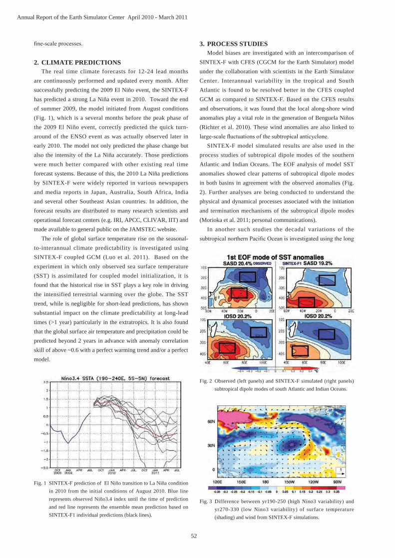
52


fine-scale processes.

2. CLIMATE PREDICTIONS The real time climate forecasts for 12-24 lead months

are continuously performed and updated every month. After successfully predicting the 2009 El Niño event, the SINTEX-F has predicted a strong La Niña event in 2010. Toward the end of summer 2009, the model initiated from August conditions (Fig. 1), which is a several months before the peak phase of the 2009 El Niño event, correctly predicted the quick turn-around of the ENSO event as was actually observed later in early 2010. The model not only predicted the phase change but also the intensity of the La Niña accurately. Those predictions were much better compared with other existing real time forecast systems. Because of this, the 2010 La Niña predictions by SINTEX-F were widely reported in various newspapers and media reports in Japan, Australia, South Africa, India and several other Southeast Asian countries. In addition, the forecast results are distributed to many research scientists and operational forecast centers (e.g. IRI, APCC, CLIVAR, IIT) and made available to general public on the JAMSTEC website.

The role of global surface temperature rise on the seasonal-to-interannual climate predictability is investigated using SINTEX-F coupled GCM (Luo et al. 2011). Based on the experiment in which only observed sea surface temperature (SST) is assimilated for coupled model initialization, it is found that the historical rise in SST plays a key role in driving the intensified terrestrial warming over the globe. The SST trend, while is negligible for short-lead predictions, has shown substantial impact on the climate predictability at long-lead times (>1 year) particularly in the extratropics. It is also found that the global surface air temperature and precipitation could be predicted beyond 2 years in advance with anomaly correlation skill of above ~0.6 with a perfect warming trend and/or a perfect model.

3. PROCESS STUDIESModel biases are investigated with an intercomparison of

SINTEX-F with CFES (CGCM for the Earth Simulator) model under the collaboration with scientists in the Earth Simulator Center. Interannual variability in the tropical and South Atlantic is found to be resolved better in the CFES coupled GCM as compared to SINTEX-F. Based on the CFES results and observations, it was found that the local along-shore wind anomalies play a vital role in the generation of Benguela Niños (Richter et al. 2010). These wind anomalies are also linked to large-scale fluctuations of the subtropical anticyclone.

SINTEX-F model simulated results are also used in the process studies of subtropical dipole modes of the southern Atlantic and Indian Oceans. The EOF analysis of model SST anomalies showed clear patterns of subtropical dipole modes in both basins in agreement with the observed anomalies (Fig. 2). Further analyses are being conducted to understand the physical and dynamical processes associated with the initiation and termination mechanisms of the subtropical dipole modes (Morioka et al. 2011; personal communications).

In another such studies the decadal variations of the subtropical northern Pacific Ocean is investigated using the long

Fig. 1 SINTEX-F prediction of El Niño transition to La Niña condition in 2010 from the initial conditions of August 2010. Blue line represents observed Niño3.4 index until the time of prediction and red line represents the ensemble mean prediction based on SINTEX-F1 individual predictions (black lines).

Fig. 2 Observed (left panels) and SINTEX-F simulated (right panels) subtropical dipole modes of south Atlantic and Indian Oceans.

Fig. 3 Difference between yr190-250 (high Nino3 variability) and yr270-330 (low Nino3 variability) of surface temperature (shading) and wind from SINTEX-F simulations.

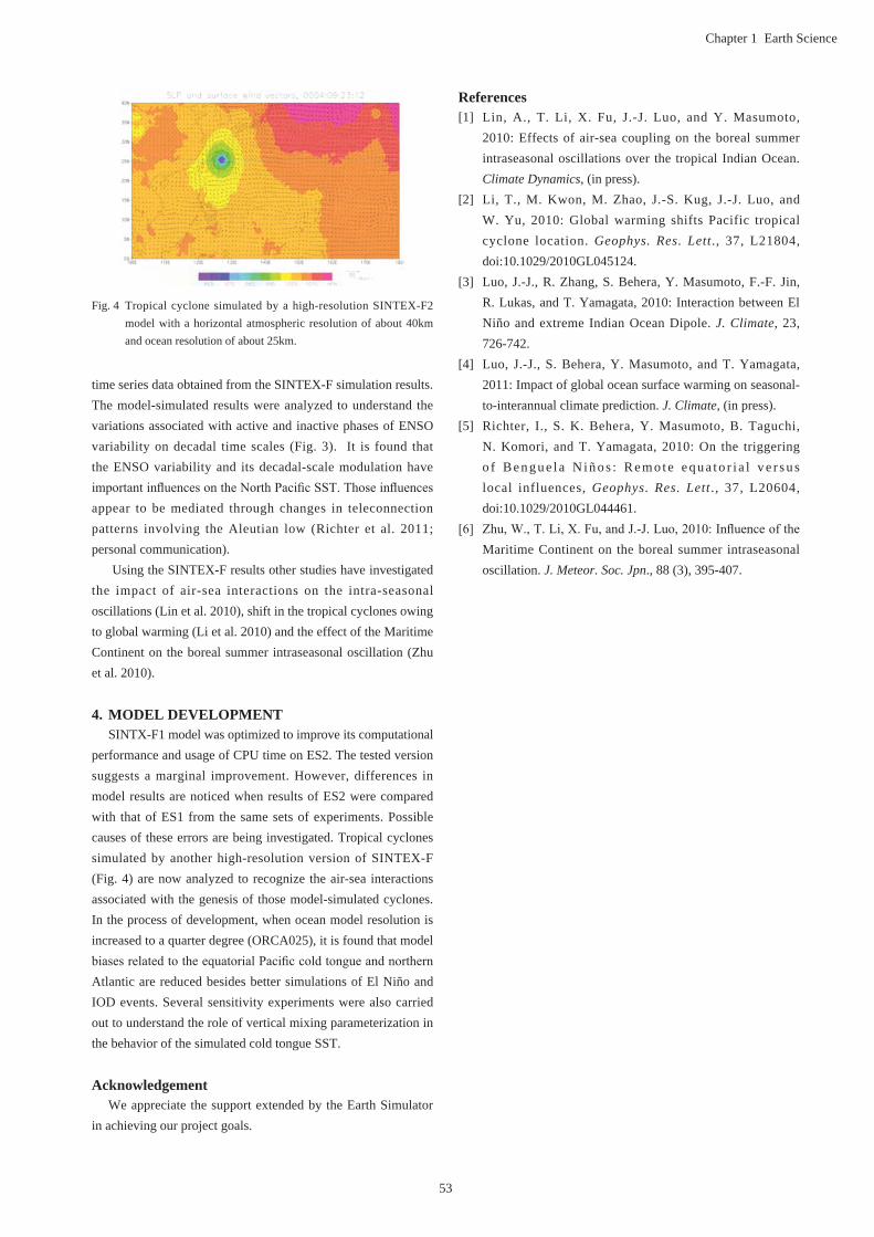
53


time series data obtained from the SINTEX-F simulation results. The model-simulated results were analyzed to understand the variations associated with active and inactive phases of ENSO variability on decadal time scales (Fig. 3). It is found that the ENSO variability and its decadal-scale modulation have important influences on the North Pacific SST. Those influences appear to be mediated through changes in teleconnection patterns involving the Aleutian low (Richter et al. 2011; personal communication).

Using the SINTEX-F results other studies have investigated the impact of air-sea interactions on the intra-seasonal oscillations (Lin et al. 2010), shift in the tropical cyclones owing to global warming (Li et al. 2010) and the effect of the Maritime Continent on the boreal summer intraseasonal oscillation (Zhu et al. 2010).

4. MODEL DEVELOPMENT

SINTX-F1 model was optimized to improve its computational performance and usage of CPU time on ES2. The tested version suggests a marginal improvement. However, differences in model results are noticed when results of ES2 were compared with that of ES1 from the same sets of experiments. Possible causes of these errors are being investigated. Tropical cyclones simulated by another high-resolution version of SINTEX-F (Fig. 4) are now analyzed to recognize the air-sea interactions associated with the genesis of those model-simulated cyclones. In the process of development, when ocean model resolution is increased to a quarter degree (ORCA025), it is found that model biases related to the equatorial Pacific cold tongue and northern Atlantic are reduced besides better simulations of El Niño and IOD events. Several sensitivity experiments were also carried out to understand the role of vertical mixing parameterization in the behavior of the simulated cold tongue SST.

AcknowledgementWe appreciate the support extended by the Earth Simulator

in achieving our project goals.

References[1] Lin, A., T. Li, X. Fu, J.-J. Luo, and Y. Masumoto,

2010: Effects of air-sea coupling on the boreal summer intraseasonal oscillations over the tropical Indian Ocean. Climate Dynamics, (in press).

[2] Li, T., M. Kwon, M. Zhao, J.-S. Kug, J.-J. Luo, and W. Yu, 2010: Global warming shifts Pacific tropical cyclone location. Geophys. Res. Lett., 37, L21804, doi:10.1029/2010GL045124.

[3] Luo, J.-J., R. Zhang, S. Behera, Y. Masumoto, F.-F. Jin, R. Lukas, and T. Yamagata, 2010: Interaction between El Niño and extreme Indian Ocean Dipole. J. Climate, 23, 726-742.

[4] Luo, J.-J., S. Behera, Y. Masumoto, and T. Yamagata, 2011: Impact of global ocean surface warming on seasonal-to-interannual climate prediction. J. Climate, (in press).

[5] Richter, I., S. K. Behera, Y. Masumoto, B. Taguchi, N. Komori, and T. Yamagata, 2010: On the triggering o f B e n g u e l a N i ñ o s : R e m o t e e q u a t o r i a l v e r s u s local influences, Geophys. Res. Lett ., 37, L20604, doi:10.1029/2010GL044461.

[6] Zhu, W., T. Li, X. Fu, and J.-J. Luo, 2010: Influence of the Maritime Continent on the boreal summer intraseasonal oscillation. J. Meteor. Soc. Jpn., 88 (3), 395-407.

Fig. 4 Tropical cyclone simulated by a high-resolution SINTEX-F2 model with a horizontal atmospheric resolution of about 40km and ocean resolution of about 25km.

54


大気海洋結合モデルを用いたプロセス研究と季節予測実験


升本　順夫　　海洋研究開発機構　地球環境変動領域

著者羅　　京佳 *1,2，佐々木　亘 *2，スワディン　ベヘラ *1,2，佐久間　弘文 *1,2，タケシ　イズモ *1，Sebastien Masson*4，Antonio Navarra*3，Silvio Gualdi*3，Simona Masina*3，Alessio Bellucci*3，Annalisa Cherchi*3，Pascal Delecluse*5，Gurvan Madec*4，Claire Levy*4，Marie-Alice Foujols*4，Arnaud Caubel*4，Guy Brasseur*6，Erich Roeckner*6，Marco Giorgetta*6，Luis Kornblueh*6，Monika Esch*6，山形　俊男 *2，升本　順夫 *1


*2 海洋研究開発機構　アプリケーションラボラトリ

*3 Centro Euro-Mediterraneo per i Cambiamenti Climatici, INGV

*4 Laboratoire D'oceanographie et du Climat (LOCEAN)

*5 Meteo France

*6 Max Planck Institute for Meteorology

気候変動ならびにその予測可能性研究のための日欧研究協力に基づき、SINTEX-Frontier大気海洋結合大循環モデルの開発および改良を推進している。その第一版の SINTEX-F1は、リアルタイムの季節・経年変動予測実験に長く用いられており、近年発生した IODやエルニーニョのほとんどを現実的に予測している。特に、2010年の夏期から発達したラニーニャ現象については、エルニーニョ現象からの移行時期や振幅も含めて、発生の１年前から予測することに成功しており、オーストラリアや南アフリカでの多雨傾向を的確に予測していた。これらの成果は国内外のメディア等で取り上げられると同時に、世界の気候変動予測研究を先導するモデルとして SINTEX-Fの地位を確立する礎となっている。また、SINTEX-F1モデルは気候変動のメカニズムを解明するための感度実験などにも利用されている。特に今年度は、

インド洋熱帯域での大気海洋相互作用がその海域での季節内変動に及ぼす影響や、インド洋および大西洋の亜熱帯ダイポールモード現象の再現性と南アフリカ域の気候変動に与える影響等の研究を進めた。その結果、亜熱帯ダイポールモード現象の発生には、海洋の表層混合層と大気との相互作用が重要であることや、気候変化に伴い太平洋域での熱帯低気圧の発生領域がこれまでよりも東へ移動することを示した。

キーワード : SINTEX-F, IOD, ENSO, 予測 , 2010年ラニーニャ現象

55


1. IntroductionThe intensive precipitation in tropics is not only a

prominent local phenomenon but also affects the planetary-scale atmospheric circulation. The Maritime Continent is one of well-known heavy-rainfall areas. It is now widely accepted that most precipitation over the Maritime Continent is caused by a convective precipitation system in synchronization with a diurnal cycle. However, in most of GCMs, the diurnal cycle, intensity and space distribution of deep convection is not well simulated. Therefore, it is an important task to understand the dynamical aspects of such deep convective systems in relation with the diurnal cycle and local circulation.

The purpose of this project is as follows; • todevelopaeddy-permittingregionalatmosphericmodel,

which can simulate turbulent motion with deep moist convection,bytheuseofagridresolutionontheorderofahundred meters, in order to represent explicitly the cloud-scale processes,

• to perform severalLarge-EddySimulation (LES)s fortropicalconvectionusing thismodel,and to improve themodel by comparing the resultswith observation andperformingsomesensitivitystudies,and

• to investigate thegenerationandmaintenancemechanism

of convective systems by the use of simulated data, which willbearranged intoadataset for theuseof improvingthecumulusparameterizationschemesusedin largerscalemodels like GCMs. Fortheeddy-permittingregionalatmosphericmodel,weare

developingamodelbasedonaglobalcloud-resolvingmodelcalledNICAM (Nonhydrostatic ICosahedralAtmosphericModel,Satohetal.,2008[1]). Thedevelopingprocess in thisyear will be shown in section 3.

Ontheotherhand,weare trying tosimulateaconvectivesystemintropicsusingexistingmodelsalreadyusedonEarthSimulator, because some of the physical schemes, such as cloud microphysics scheme and turbulent closure scheme, can be testedandimprovedinthesemodelsbeforewefinishdevelopingoureddy-permittingregionalatmosphericmodel.TheresultsoftheexperimentsusingastretchedgridsystemofNICAMwillbe shown in section 2.

2. Preliminary experiment toward LES of deep convective systemsAspreliminariesofLESofdeepconvectivesystems,apartof

objectives at this research project, we conducted an experiment fordeepconvectivecloudsusingastretchedgridsystemof

Simulation and Verification of Tropical Deep Convective Clouds using Eddy-Permitting Regional Atmospheric Models


Kozo Nakamura ResearchInstituteforGlobalChange,JapanAgencyforMarine-EarthScienceandTechnology

Authors

Kozo Nakamura*1, Yasutaka Wakazuki*1, Masayuki Hara*1, Akira T. Noda*1 and Hirofumi Tomita*1,2

*1 ResearchInstituteforGlobalChange,JapanAgencyforMarine-EarthScienceandTechnology


Wearedevelopinganeddy-permittingregionalatmosphericmodel,whichcansimulate turbulentmotionwithdeepmoistconvection.Inordertodevelopamodelefficiently,weadoptedamodelusingsimilardynamicalandphysicalframeworkstothoseofaglobalcloud-resolvingmodelcalledNICAM(NonhydrostaticICosahedralAtmosphericModel).Wearemodifyingthedynamicallyallocatedarrays,communicationpatternformessagepassinginterface,andhandlingofhaloregionsintheoriginalNICAM.InFY2010,wedevelopedashallowwaterequationsystemmodelandvalidatedthemodificationforregionalmodel.Inaddition,inorderto improve the physical models such as cloud microphysical model and turbulent closure model, we started a simulation of tropical deepconvectionusingastretchedgridsystemofNICAMforthecasecalledtheTropicalWarmPoolInternationalCloudExperiment(TWP-ICE).Theresultsindicatetypicalcharacteristicsofdeepcloudsthatdevelopoveraboundarylayertoafreeatmosphere.

Keywords: LES,regionalatmosphericmodel,deepconvection,NICAM,cloudresolvingmodel

56


NICAM. The spatial resolution of the model is horizontally 2 kmatafinestgridpoint,andvertically100monaverage.Weusedlevel2ofMYNN(NakanishiandNiino2004[2];Nodaetal.2010[3]) forcomputationof thesubgrid-scale turbulence,andNSW6(Tomita2008)[4]forprocessofcloudmicrophysics,whichparameterizationschemesaregenerallybeingused incloud-resolvingsimulationsofNICAM.

ThemodelsettingweadoptedisthecasecalledtheTropicalWarmPoolInternationalCloudExperiment(TWP-ICE,Mayetal.2008[5]),amajorfieldexperimentundertakenintheDarwin,NorthernAustralia,areainJanuaryandFebruary2006.Inthefineresolutiondomain,whichcoversapproximately(500km)2 area, thehorizontalgridintervalusedis less than5kminthestretchedgridsystem.

Figure1 shows the temporal evolutionof apreliminaryexperiment of a cloud system in a typical tropical environment. The model simulates well typical deep clouds that develop over a boundary layer to a free atmosphere with the simulation time elapses. The cloud system becomes in a nearly equilibrium state after 6 hrs, and it maintains steady thereafter.

Figure2 comparesvertical distributionsof condensatesafter 12 hrs. The cloud ice distributes beneath and rightbelowa tropopause (~20kmaltitude), and the snowwater,whichdevelops throughaccretionandcollectionprocesses,distributesunderneath it.Thegraupelevolves furtherbelowthe layer, because its fall velocity is faster due to its heaviness. Thesesolidwaterspeciesgrowfurther throughaccretionandcollectionprocessesduringfall,andeventuallybecomestherainwaterbelow6kmaltitude,afreezinglevel.Thecloudwaterismaintainedevenabovethefreezinglevelasmixedphaseclouds.

Wewill undertakedevelopingaLESmodelbasedonaNICAM framework, and explore detailed behavior of tropical deep convective systems in the future obtained by means of LES.

3. New regional climate model based on a global cloud-resolving modelWearedevelopinganewregionalclimatemodelbasedona

globalcloud-resolvingmodel,i.e.NICAM[1]thatisdevelopingincooperationwithRIGC,JAMSTECandAORI,University

ofTokyo.Simulationdomainofthenewlydevelopedregionalmodel (hereafter regionalNICAM)consistsofonediamond(twotrianglesinanicosahedron),althoughtheoriginalNICAMglobaldomainconsistsoftendiamonds(twentytriangles)(Fig.3).Thisapproachbringsfollowingadvantages todevelopersand users.(i) SharingsoftwareframeworkbetweentheoriginalNICAM

andtheregionalNICAM,(ii) SeamlessnestingfromtheoriginalNICAMtotheregional

NICAM,(samedynamicalequationsystemand/orphysicsschemes),

(iii)Identifieduser landbetween theoriginalNICAMandthe regionalNICAM(onceyou learnhow toperform

Fig.2 Verticaldistributionofsimulatedcondensates.Fromlefttoright,horizontalmeansofmixingratios(10mgkg-1)forcloudwater,cloudice,graupel,snowwater,andrainwater.Thevaluesareaveragedoverafineresolutiondomain,thehorizontalresolutionofwhichishigherthanapproximately5km.

Fig.1 Temporalevolutionofsimulateddeepconvectivesystems.Fromtop tobottom,horizontalmeansmixing ratios (mgkg-1) forcloudwater,cloudice,graupel,snowwater,andrainwater.Thevaluesareaveragedoverafineresolutiondomain,thehorizontalresolutionofwhichishigherthanapproximately5km.

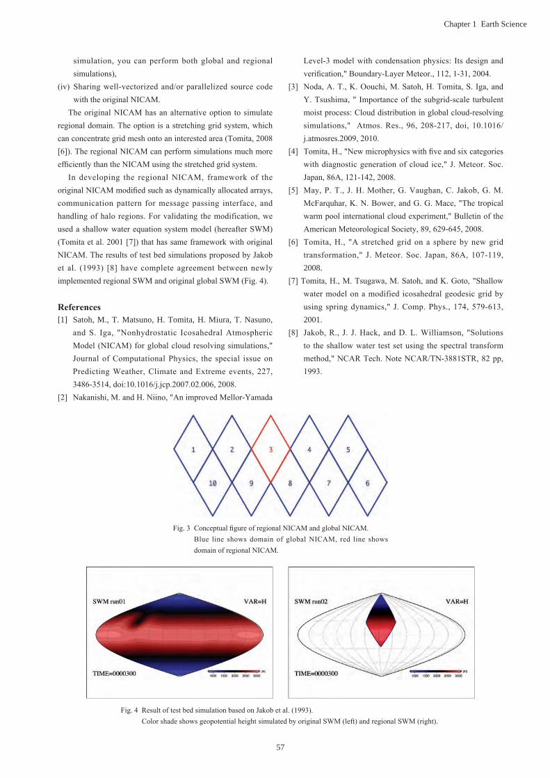
57


simulation,you canperformbothglobal and regionalsimulations),

(iv) Sharingwell-vectorizedand/orparallelizedsourcecodewiththeoriginalNICAM.

TheoriginalNICAMhasanalternativeoption tosimulateregionaldomain.Theoptionisastretchinggridsystem,whichcanconcentrategridmeshontoaninterestedarea(Tomita,2008[6]).TheregionalNICAMcanperformsimulationsmuchmoreefficientlythantheNICAMusingthestretchedgridsystem.

In developing the regionalNICAM, framework of theoriginalNICAMmodifiedsuchasdynamicallyallocatedarrays,communicationpattern formessagepassing interface, andhandlingofhaloregions.Forvalidating themodification,weusedashallowwaterequationsystemmodel(hereafterSWM)(Tomitaetal.2001[7])thathassameframeworkwithoriginalNICAM.TheresultsoftestbedsimulationsproposedbyJakobet al. (1993) [8] have complete agreementbetweennewlyimplementedregionalSWMandoriginalglobalSWM(Fig.4).

References [1] Satoh, M., T. Matsuno, H. Tomita, H. Miura, T. Nasuno,

andS. Iga, "Nonhydrostatic IcosahedralAtmosphericModel(NICAM)forglobalcloudresolvingsimulations,"JournalofComputationalPhysics, the special issueonPredictingWeather,ClimateandExtremeevents,227,3486-3514,doi:10.1016/j.jcp.2007.02.006,2008.

[2] Nakanishi,M.andH.Niino,"AnimprovedMellor-Yamada

Level-3modelwithcondensationphysics: Itsdesignandverification,"Boundary-LayerMeteor.,112,1-31,2004.

[3] Noda,A.T.,K.Oouchi,M.Satoh,H.Tomita,S.Iga,andY.Tsushima,"Importanceof thesubgrid-scale turbulentmoistprocess:Clouddistributioninglobalcloud-resolvingsimulations," Atmos.Res.,96,208-217,doi,10.1016/j.atmosres.2009,2010.

[4] Tomita,H.,"Newmicrophysicswithfiveandsixcategorieswithdiagnosticgenerationofcloudice,"J.Meteor.Soc.Japan,86A,121-142,2008.

[5] May,P.T., J.H.Mother,G.Vaughan,C.Jakob,G.M.McFarquhar,K.N.Bower,andG.G.Mace,"Thetropicalwarmpoolinternationalcloudexperiment,"BulletinoftheAmericanMeteorologicalSociety,89,629-645,2008.

[6] Tomita,H., "Astretchedgridona spherebynewgridtransformation," J.Meteor.Soc. Japan,86A,107-119,2008.

[7]Tomita,H.,M.Tsugawa,M.Satoh,andK.Goto,"Shallowwatermodelonamodified icosahedralgeodesicgridbyusingspringdynamics," J.Comp.Phys.,174,579-613,2001.

[8] Jakob,R., J. J.Hack,andD.L.Williamson,"Solutionsto theshallowwater testsetusing thespectral transformmethod,"NCARTech.NoteNCAR/TN-3881STR,82pp,1993.

Fig.3 ConceptualfigureofregionalNICAMandglobalNICAM. Blue line showsdomainof globalNICAM, red line shows

domainofregionalNICAM.

Fig.4 ResultoftestbedsimulationbasedonJakobetal.(1993). ColorshadeshowsgeopotentialheightsimulatedbyoriginalSWM(left)andregionalSWM(right).

58


渦解像可能な領域大気モデルを用いた深い対流のシミュレーションとその検証


中村　晃三　　海洋研究開発機構　地球環境変動領域

著者中村　晃三 *1，若月　泰孝 *1，原　　政之 *1，野田　　暁 *1，富田　浩文 *1,2



十分に細かい格子を用い、深い湿潤対流を解像できるモデルを開発している。効率的な開発のため、全球雲解像モデル（NICAM、Nonhydrostatic ICosahedral Atmospheric Model）と共通の力学／物理フレームワークを用いた領域版 NICAMモデルを採用した。今年度は、領域版 NICAMの開発においては浅水方程式モデルでのチェックを行った。同時に、モデルに搭載する雲微物理モデルや乱流モデルなどの物理過程モデルの改良のために、既存のストレッチ版 NICAMを用い、深い対流の再現実験を始め、良好な結果を得た。

キーワード : LES, 領域大気モデル , 深い対流 , NICAM, 雲解像モデル

59


1. IntroductionNitrous oxide (N2O) in the troposphere is an important

g reenhouse gas an th ropogen ica l ly enhanced s ince industrialization starting in the 19th century, accounting for about 5% of radiative forcing in the troposphere except water vapor (Forster et al., 2007). N2O is also regarded as the most influential ozone depleting substance (ODS) being an exclusive source of nitrogen oxide (NO) in the stratosphere in this century (Ravishankara et al., 2009). However, it is difficult to immediately reduce N2O emission because the main source of anthropogenic N2O is agricultural activities (e.g. fertilization) to feed increasing population on the globe and the atmospheric lifetime of N2O is more than a hundred years (114 years) (Forster et al., 2007). Quantitative details of N2O emission from various natural and anthropogenic sources are still quite uncertain on regional to global scales despite much effort of the bottom-up and top-down estimations in the past. N2O also has five different isotopologues with the mass of 44, 45, 46, 47 and 48, and some isotopomers in each isotopologues. The isotopomers are very useful to know origin of the N2O, because individual isotopomers show different behaviors in biogeochemical processes, due to differences of the mass and of the molecular location. 14N14N16O, 14N15N16O, 15N14N16O , and 14N14N18O account more than 99.9% of all N2O species. There are many observation studies for them, but only a few global modeling studies to understand the observed results. In this

study, we simulated these four isotopomers as different tracers for understanding N2O behaviours in both the stratosphere and the troposphere, using an atmospheric general circulation model driven chemistry transport model.

2. Model descriptionWe have developed an atmospheric chemical transport

model (ACTM) based on the CCSR/NIES/FRCGC atmospheric general circulation model (AGCM) to simulate atmospheric N2O concentration and its isotopes. A detailed and consistent meteorology as represented by the grid- and subgrid-scale processes, surface processes (e.g. PBL height and mixing), above-PBL dynamics (e.g. convection) were generated by the AGCM. The meteorological field in the AGCM was assimilated with the European Center for Medium-range Weather Forecasts (ECMWF) 40 year reanalysis and National Centers for Environmental Prediction (NCEP) version 2 reanalysis data via nudging for the comparison of temporal variations of N2O and its isotopologues with ground-based and air-bourne observations. We use T42 truncation in the horizontal and 67 vertical sigma-pressure layers up to 90 km for the present study. Feedbacks between dynamics-radiation-chemistry are taken into account in the model. For example, the photolysis rate of N2O is estimated by using the shortwave radiative flux calculated in the radiation scheme of the model, and the radiation flux is calculated with cloud distribution and temperature in each

Estimation of the Variation of Atmospheric Composition and Its Effect on the Climate Change by using a Chemical Transport Model


Masayuki Takigawa Research Institute for Global Change, Japan Agency for Marine-Earth Science and Technology

Authors

Kentaro Ishijima*1, Masayuki Takigawa*1 and Prabir K. Patra*1

*1 Research Institute for Global Change, Japan Agency for Marine Earth Science and Technology

An online chemical transport model that can estimate the global distributions of N2O isotopomers in the stratosphere and the troposphere has been developed. Fractionation of isotopes during the photolysis and chemical reactions was estimated by using the temperature and radiative flux estimated in the model. To estimate the global distribution of N2O and its isotopomers, 20-years calculations have been executed. The isotopomers fractions in the emissions were estimated by assuming the isotopic fractions in various sources. The model well reproduced the vertical gradient of N2O concentration and the isotopomers fractions observed at Sanriku, Kiruna, and Showa-station. The averaged value of the isotopomers fraction in the model was close to that from the emissions from the anthropogenic emissions, especially cultivated soil.

Keywords: greenhouse gases, isotopes, general circulation of atmospheric composition, chemical transport model

60


model time step (typically 20 minutes).N2O (14N14N16O) inventory consists of three components of

anthropogenic (Emission Database for Global Atmospheric Research (EDGAR) version 3.2 Fast Track 2000, annual mean), ocean (Global Emission Inventory Activity (GEIA), monthly mean) and soil (EDGAR version 2.0, annual mean) emissions. Inventories for isotopomers were estimated by applying isotopic values of anthropogenic and natural sources by Röckmann et al. (2003) and Ishijima et al. (2007). Fractionation coefficients in photolysis were incorporated, using experimental results by Kaiser et al. (2002, 2003) and von Hessberg et al. (2004). For fractionation in oxidation, coefficient values by Kaiser et al. (2002) were implemented. Dependencies on wavelength and temperature were considered for all isotopic fractionations. Parameterization lines for fractionation constants, which were originally calculated following to von Hessberg et al. (2004) with a factor of 1.2 for the better representations of observational variations within the range of uncertainty of the fractionation parameterisation.

3. Result and discussionWe have prepared two emission scenarios and two initial

values for each isotopomers: each isotopomer has four historical cases in a model run to cover ranges of observed N2O concentration and isotopomer ratios at the Neumayer station. Isotopomer ratios of 14N15N16O, 15N14N16O, 14N14N18O are denoted by δ15Ncentral, δ15Nterminal, and δ18O in permil unit (‰), respectively. Here, δ=(R/Rreference-1) x 103 (R=[N2O]/[N2O]standard). For the estimation of source of emissions, following denotations are also used; δ15NBulk=(δ15Ncentral+δ15terminal)/2 and SP=δ15Ncentral–

δ15Nterminal.Vertical profiles of observed and modeled concentration

of N2O and ratio of isotopomers at three stations (Sanriku, Kiruna, and Showa) are shown in Fig. 1. General features of N2O concentration (e.g. vertical gradient) observed using balloon are well captured by the model, but fine structures are not well simulated. For example, the model cannot reproduce steep decrease of N2O concentration at around the height of 20km at Sanriku, which was corresponding with the eventual intrusion of upper stratospheric air. The difference of meteorological field (NCEP2 and ERA40) does not strongly affect the vertical profiles of N2O concentration. Model also roughly reproduces observed isotopomer ratios. Rayleigh plots show that N2O isotopic fractionations caused by stratospheric chemical reactions are well simulated, although the fractionation of δ15Nterminal seem to be underestimated in almost cases. Model significantly underestimates the concentration and the fractionation over Kiruna, indicating the air-age is younger than real in the polar vortex in boreal winter, which is not realistically reproduced by this model.

δ15NBulk and SP estimated in this study is shown in Fig. 2, with the observed values from various sources (Toyoda et al., 2004). It seems that δ15NBulk and SP for global total N2O sources estimated in this study are reasonably in the range of measured values for land sources (temperate soil and cultivated soil). It is possible that model overestimate isotopomer ratios in the global total sources, because model tends to overestimate heavier isotopomers losses in the stratosphere, which causes underestimation in isotopomer ratios.

Fig. 1 Comparison of N2O concentration, δ15Nterminal, δ15Ncentral and δ18O, and Rayleigh plots of the isotopomers between balloon observations over Sanriku (39N, 142E, Japan), Kiruna (68N, 20E, Sweden) and Syowa (69S, 40E, Antarctica), and the model results. NC2, ERA and NC2s represent simulation assimilated with NCEP2, ERA-40 and NCEP2+ fractionation multiplied by 1.2, respectively.

61


4. SummaryAn online chemical transport model that can estimate the

global distributions of N2O isotopomers in the stratosphere and the troposphere has been developed. Fractionation of isotopes during the photolysis and chemical reactions was estimated by using the temperature and radiative flux estimated in the model. To estimate the global distribution of N2O and its isotopomers, 20-years calculations have been executed. The isotopomers fractions in the emissions were estimated by assuming the isotopic fractions in various sources. The model well reproduced the vertical gradient of N2O concentration and the isotopomers fractions observed at Sanriku, Kiruna, and Showa-station. The averaged value of the isotopomers fraction in the model was close to that from the emissions from the anthropogenic emissions, especially cultivated soil.

References[1] Forster, P., V. Ramaswamy, P. Artaxo, T. Berntsen, R.

Betts, and co-authors, Changes in Atmospheric Constituents and in Radiative Forcing. In: Climate Change 2007: The Physical Science Basis. Contribution of Working Group I to the Fourth Assessment Report of the Intergovernmental Panel on Climate Change. Cambridge University Press, Cambridge, United Kingdom and New York, NY, USA, 2007.

[2] Ravishankara A. R., J. S. Daniel, and R. W. Portmann, Nitrous Oxide (N2O): The dominant ozone-depleting substance emitted in the 21st century, Science, 326(5949), 123-125, 2009.

[3] Röckmann, T. and I. Levin, High-precision determination of the changing isotopic composition of atmospheric N2O from 1990 to 2002, J. Geophys. Res., 110, D21304, doi:10.1029/2005JD006066, 2005.

[4] Ishijima, K., P. K. Patra, M. Takigawa, T. Machida, H. Matsueda, Y. Sawa, L. P. Steele, P. B. Krummel, R. L. Langenfelds, S. Aoki, and T. Nakazawa, Stratospheric influence on the seasonal cycle of nitrous oxide in the troposphere as deduced from aircraft observations and model simulations, J. Geophys. Res., 115, D20308, doi:10.1029/2009JD013322, 2010.

[5] Kaiser et al., Phys. Chem. Chem. Phys., 4(18), 4420-4430, 2002.

[6] Kaiser et al., Atmos. Chem. Phys., 3, 303-313, 2003.[7] von Hessberg et al., Atmos. Chem. Phys., 4, 1237-1253,

2004.[8] Toyoda e t a l . , J . Geophys . Res . , 109 , D08308 ,

doi:10.1029/2003JD004316, 2004.

Fig. 2 δ15NBulk and SP for global total N2O sources estimated in this study (blue and red squares). The measurement value ranges for various sources (Toyoda et al. 2004) are also shown for comparison.

62


化学輸送モデルによる大気組成変動と気候影響の研究


滝川　雅之　　海洋研究開発機構　地球環境変動領域

著者石島健太郎 *1，滝川　雅之 *1，プラビール・パトラ *1


地球温暖化およびそれに伴う気候変動に大きな影響を与えると考えられる温室効果気体の大気中濃度変動を解析するため、大気大循環モデルMIROCを基にした温室効果気体に特化した化学輸送モデル ACTMを開発した。温室効果気体のソース・シンク、および輸送過程に関する評価を行うため、一酸化二窒素の同位体を用いた地表放出源分布推定および輸送過程等の検証を行った。地表観測値と ACTMによる複数の第一推定値とを組み合わせて現在気候および産業化以前における地表放出源における全球平均した一酸化二窒素アイソトポマー比の推定を行った結果、モデルが北半球高緯度、中緯度および南極昭和基地でのアイソトポマー比の鉛直分布等を良く再現していること、およびδ 15Nbulk（N15存在比）や SP（N15が終端に存在する比率）、δ 18Oなどの値から、人為起源放出源、とくに農耕地の N2Oアイソトポマー比に近いことなどが明らかとなった。

キーワード : 大気物質循環 , 温室効果気体 , 化学輸送モデル , 同位体

63


1. IntroductionData assimilation approaches have recently focused on the

derivation of an optimal synthesis of observational data and model results for better descriptions of the ocean state [1]. The synthesis efforts so far have mainly directed the attention to the upper ocean since observations of changes in the properties of ocean waters have been restricted to surface or intermediate-depth waters.

Based on high quality observational survey, recent studies have found the sobering fact that the deepest waters of the major ocean have warmed significantly during the recent decades [2]. This bottom-water warming is of particular interest as they can constrain estimates of the variability of abyssal circulation. The latter have implications for large-scale thermohaline transport and thus for the global 3-dimensional heat budget that is presently of vital concern in conjunction with climate warming.

In this study, we will take the deepest waters into consideration through data assimilation procedure in order to more precisely assess various climate variabilities.

2. ModelThe used OGCM is based on version 3 of the GFDL Modular

Ocean Model (MOM) [3] with major physical parameter values determined through a variational optimization procedure [4]. The horizontal resolution is 1° in both latitude and longitude, and there are 46 vertical levels for the global ocean basin. The adjoint code of the OGCM was obtained using the Transformation of Algorithms in Fortran (TAF).

Our system has been executed on the Earth Simulator 2 to obtain a comprehensive 4-dimensional dataset [5]. The assimilated elements are historical hydrographic data of temperature and salinity from the ENSEMBLES (EN3) dataset which was quality-controlled using a comprehensive set of objective checks developed at the Hadley Centre of the UK Meteorological Office [6]. In addition of EN3 dataset, recent data obtained/compiled in JAMSTEC (independent MIRAI RV profiles and a climatology of subsurface 2-dimensional velocity estimated from Argo floats [7]) are simultaneously incorporated. NOAA Optimum Interpolation SST (NOAA_OI_SST_V2) values, and sea-surface dynamic-height anomaly data derived from the high-precision multi-satellite altimetry products produced by Ssalto/Duacs are also assimilated.

3. Ocean State EstimateThe assimilation is based on a 4D-VAR adjoint approach

which can precisely determine the time-trajectory of the ocean states, and thus can provide analysis fields in superb quality through 4-dimensional dynamical interpolation of in-situ observations for water temperature, salinity and sea surface height anomaly, as obtained from various instrumental sources. The analysis fields successfully capture the realistic time trajectory of ocean properties and observed patterns of ocean circulation and surface air-sea heat fluxes. For example, Fig. 1 shows estimated steric height distribution in an El Niño year. Significant sea level rises appear in the eastern equatorial Pacific and central Indian Ocean in conjunction with interannual

Improved Estimates of the Dynamical Ocean State by using a 4D-VAR Adjoint Method


Shuhei Masuda Research Institute for Global Change, Japan Agency for Marine-Earth Science and Technology

Authors

Shuhei Masuda*1, Toshiyuki Awaji*2, Nozomi Sugiura*1, Yoshihisa Hiyoshi*2, Yuji Sasaki*2 and Hiromichi Igarashi*2


*2 Data Research Center for Marine-Earth Sciences, Japan Agency for Marine-Earth Science and Technology

The spatio-temporal coverage of hydrographic data is still sparse. To obtain a 4-dimensionally continuous state estimation of the global ocean, 4-dimensional variational (4D-VAR) data assimilation system has been developed. This system is capable of providing an optimal synthesis of the observational data and a climate model by solving a nonlinear least square problem. The obtained dynamically self-consistent 4-dimensional dataset can offer greater information content on ocean climate changes than can be derived from models or data alone.

Keywords: Ocean, Data assimilation, Climate change, 4D-VAR

64


changes in oceanic heat storage. Recent-day sea level change is of considerable interest because of its potential impact on human populations living.

4. Applications to Climate ResearchBy using this ocean state estimation, the bottom-water

warming is assessed. The bottom water warming in the North Pacific is successfully reproduced in our reanalysis field (Fig. 2), which can lead to better understanding of the warming trend of the global ocean. Detailed analysis on the basis of model formalism uncovered a new finding that temporal change in the horizontal advection mainly causes variations of the local time change, implying that the changes in the abyssal circulation constrain the bottom-water warming [5].

5. Concluding RemarksBy using a 4-dimensional variational adjoint method, we

have obtained an oceanic reanalysis dataset for 1957-2006. The

reconstructed field, which has dynamical consistency, reflects most of the familiar gross features of past studies. Hence, our product is useful for understanding long-term oceanic variabilities. The dynamical analysis on the bottom-water warming led to new findings of its mechanism. Our variational data assimilation approaches, in turn, can possibly help construct an optimal observing system.

AcknowledgementWe thanks J. P. Matthews and Y. Ishikawa for helpful

discussion.

References[1] Stammer, D., C. Wunsch, I. Fukumori, and J. Marshall,

State Estimation in Modern Oceanographic Research, EOS, Transactions, American Geophysical Union, Vol. 83, Nr. 27, p. 289, 294-295, 2002.

Fig. 1 Distribution of steric sea level change for Jan 1998 (El Niño year) estimated from 4-dimensional synthesis dataset.

Fig. 2 Bottom water warming in the Pacific Ocean below 4000m-depth; (a) observed heat content trend and (b) estimated temperature trend.

65


[2] Fukasawa, M., H. Freeland, R. Perkin, T. Watanabe, H. Uchida, and A. Nishina, Bottom water warming in the North Pacific Ocean, Nature, 427, 825-827, 2004.

[3] Pacanowski, R. C. and S. M. Griffies, The MOM 3 manual, report, 680 pp., Geophys. Fluid Dyn. Lab., Princeton, N. J, 1999.

[4] Menemenlis, D., I. Fukumori, and T. Lee, Using Green's functions to calibrate an ocean general circulation model, Mon. Wea. Rev., 133, 1224-1240, 2005.

[5] Masuda, S., T. Awaji, N. Sugiura, J. P. Matthews, T. Toyoda, Y. Kawai, T. Doi, S. Kouketsu, H. Igarashi, K. Katsumata, H. Uchida, T. Kawano, and M. Fukasawa,

Simulated Rapid Warming of Abyssal North Pacific Waters, Science, 329, 319-322, DOI:10.1126/science.1188703, 2010.

[6] Ingleby, B. and M. Huddleston, Quality control of ocean temperature and salinity profiles - historical and real-time data, Journal of Marine Systems, 65, 158-175, DOI: 10.1016/j.jmarsys.2005.11.019, 2007.

[7] Katsumata, K. and H. Yoshinari, Uncertainties in Global Mapping of Argo Drift Data at the Parking Level, Journal of Oceanography, Vol. 66 (No. 4), 553-569, 2010.

66


四次元変分法海洋データ同化システムを用いた海洋環境再現実験


増田　周平　　海洋研究開発機構　地球環境変動領域

著者増田　周平 *1，淡路　敏之 *2，杉浦　望実 *1，日吉　善久 *2，佐々木祐二 *2，五十嵐弘道 *2


*2 海洋研究開発機構　地球情報研究センター

船舶、衛星観測などから得られる海洋観測データの時空間的な分布密度は地球規模の気候変動研究を進めるうえで十分に密であるとは言えない。気候変動現象をより精緻に解析するためにはデータ同化技術を用いた力学補完が有用である。本研究では四次元変分法海洋同化システムを用いて、高精度な海洋環境再現データを作成した。このデータセットを用い、深層昇温現象など地球規模での海洋環境変動の力学解明に取り組み、そのメカニズムの一端を明らかにした。

キーワード : 海洋 , データ同化 , 気候変動 , 4D-VAR

67


1. IntroductionOcean modeling at various frequency ranges has been

explored over the long term. Global ocean tide models have been developed and utilized for various geophysical purposes [1-3]. Developments of ocean models for seasonal and longer time scale variations have been increasingly conducted for studying global climate changes [4, 5]. Ocean variations at intermediate periods from days to tens of days due to synoptic atmospheric disturbances can be modeled by barotropic ocean models [6, 7]. Accuracy of the modeling seems insufficient to correcting oceanic components from geodetic measurement data. In the present study, we address to increase realism of the modeling of the high-frequency, synoptic-disturbance-induced ocean variations for detecting vertical crustal deformation of centimeters at the frequency from OBP (ocean bottom pressure) observations [8, 9].

2. Model descriptionA non-linear, single-layer shallow-water model in a spherical

coordinate [10, 11] is used to simulate vertically-integrated velocity and sea level. Governing equations are as follows:

дv + (v�

Δ

)v + f × v =

Δ(-gƞ +P ) +

τ ‒ γb

v|v|+AH

Δ2vдt ρ ρH H

(1)

дƞ

+

Δ

�(vH) = 0дt

(2)

τ =ρaCdW|W| (3)where v and η are horizontal velocity and sea level anomaly, respectively. H is water column height which is equal to the sea level anomaly plus depth. Surface air pressure and wind stress vector are denoted by P and τ, respectively. f, g, and ρ are Coriolis parameter, gravity acceleration, and seawater density, respectively. Friction terms are parameterized by two coefficients: γb for quadratic bottom drag, AH for horizontal eddy viscosity. Wind stress on sea surface is converted from quadratic wind speed (W) through bulk coefficient (Cd). ρa is air density. The partial differential equations are discretized by a second-order finite-difference scheme on the staggered Arakawa-C grid system using a control volume formalism, with a potential energy and enstrophy-conserving scheme [12]. Time integration is accomplished using a second-order leapfrog scheme associated with the Asselin filter [13] to suppress high-frequency numerical noises.

Global ocean modeling is carried out in the present study for general versatilities of the modeling. An easy coordinate transformation performed by Yoshida and Hirose [14] is applied retaining the latitude/longitude coordinate so as to calculate the global ocean including Arctic Ocean (Fig. 1). Singular poles are both located on lands (China/Argentine) in the transformed coordinate. The difference equations keep unchanged by the coordinate transformation, which is a merit of this method. The modeled ocean is driven by global 6-hourly atmospheric

Realistic High-Frequency Global Barotropic Ocean Modeling Driven by Synoptic Atmospheric Disturbances


Ryota Hino Research Center for Prediction of Earthquakes and Volcanic Eruptions, Graduate School of Science, Tohoku University

Authors

Daisuke Inazu*1, Ryota Hino*1 and Hiromi Fujimoto*1

*1 Research Center for Prediction of Earthquakes and Volcanic Eruptions, Graduate School of Science, Tohoku University

In this project we develop realistic global barotropic ocean modeling for the high-frequency (O(day-1)) ocean variation induced by synoptic atmospheric disturbances. A number of numerical experiments reveal that the model results strongly depend on the horizontal resolution of the modeling. The model accuracy is validated by global in-situ 144 OBP (ocean bottom pressure) data, and is shown to be highest when the model resolution is 1/12°. The model skill yields a correlation coefficient of 0.55 to the observation on global average at the period longer than 2 days. However, finer resolution models show lower model skills with smaller OBP amplitude than the observation. This deficiency is probably caused by inadequacy of barotropic assumption in the modeling. The barotropic model would not represent energy distribution processes due to baroclinic instability that should be effective at spatial scales less than tens of kilometers.

Keywords: global barotropic ocean model, synoptic atmospheric disturbances, ocean bottom pressure, horizontal resolution

68


reanalysis data: surface air pressure (P) and wind vector (W). Bathymetry and coastlines are given by global bathymetric data.

3. Numerical experimentsThe parameters below are variable in the modeling, and

tuned for realistic modeling.a) Implicit parameter: horizontal resolution.b) Explicit parameters: atmospheric reanalysis data (P and W),

bathymetric data, Cd, γb, and AH.

a) Horizontal resolution: Numerical simulations with horizontal resolutions of 1/2°, 1/4°, 1/6°, 1/10°, 1/12°, 1/15°, 1/20°, and 1/30° are carried out, respectively.

b-1) Atmospheric reanalysis data: Atmospheric forcing is given by ERA-Interim [15], JRA-25 [16], NCEP [17], and NCEP2 [18], respectively.

b-2) Bathymetry: Bathymetry and coastlines are given by GEBCO_08 [19] or ETOPO1 [20].

b-3) Cd: Several formulations are provided by Powell et al. [21], Donelan et al. [22], and Black et al. [23].

b-4) γb: A uniform formulation over the model domain is adopted.

b-5) AH: An isotropic formulation (uniform over the model domain) is adopted.

Sensitivities of the model results to above the boundary conditions and the parameters are examined.

4. Model dependence on horizontal resolutionSimulated variabilities are found to strongly depend on the

horizontal resolution. The OBP variabilities become smaller in most regions when finer resolution modeling is conducted although there are exceptions in coastal and marginal seas (Fig. 2). This result is probably caused by dependence of frictional energy dissipation on the horizontal resolution. It is expected that the dissipation of the kinetic energy due to bottom friction is small for smoothed bathymetry in coarse resolutions, but is large for steep bathymetry in fine resolutions, as pointed by Hirose et al. [6].

5. Model validation using global in-situ OBP dataAccuracy of the modeling is validated by in-situ OBP data

over global ocean. The number of the data is 144. The model skill is evaluated by correlation coefficient between the observed

Fig. 1 Transformed latitude/longitude coordinate. Contour intervals are 10 degrees.

-90

-60

-30

0

30

60

90

Latit

ude

(°N

)

0 30 60 90 120 150 180 210 240 270 300 330 360

Longitude (°E)

-90

-60

-30

0

30

60

90

Latit

ude

(°N

)

0 30 60 90 120 150 180 210 240 270 300 330 360

Longitude (°E)

-90

-60

-30

0

30

60

90

Latit

ude

(°N

)

0 30 60 90 120 150 180 210 240 270 300 330 360

Longitude (°E)

-90

-60

-30

0

30

60

90

Latit

ude

(°N

)

0 30 60 90 120 150 180 210 240 270 300 330 360

Longitude (°E)

-90

-60

-30

0

30

60

90

Latit

ude

(°N

)

0 30 60 90 120 150 180 210 240 270 300 330 360

Longitude (°E)

Fig. 2 Standard deviation of the simulated OBP. The results are shown when the horizontal resolution is (a) 1/6°, (b) 1/12°, and (c) 1/30°.

-90

-60

-30

0

30

60

90

Latit

ude

(°N

)

0 30 60 90 120 150 180 210 240 270 300 330 360

Longitude (°E)

-90

-60

-30

0

30

60

90

Latit

ude

(°N

)

0 30 60 90 120 150 180 210 240 270 300 330 360

Longitude (°E)

0 2 4 6 8 10 12 14

hPa

0 30 60 90 120 150 180 210 240 270 300 330 360

Longitude (°E)

0 30 60 90 120 150 180 210 240 270 300 330 360

Longitude (°E)

0 2 4 6 8 10 12 14

hPa

0 30 60 90 120 150 180 210 240 270 300 330 360

Longitude (°E)

0 30 60 90 120 150 180 210 240 270 300 330 360

Longitude (°E)

0 2 4 6 8 10 12 14

hPa

(a) (b) (c)

69


and the simulated OBP on global average. The correlation coefficient is calculated from the time series at the period longer than 2 days. Figure 3 shows dependence of the model skill on the horizontal resolution. The model skill is highest when the horizontal resolution is 1/12°, but worsens in either case of finer or coarser resolution. The modification of the horizontal resolution yields the model skill changes of the correlation coefficient of the order of 0.1. Simulated OBP amplitudes in the cases of horizontal resolutions finer than 1/12° are smaller than the observed OBP amplitude. Other parameter changes yield the correlation coefficient changes only of the order of 0.01. In the next section, the model skill of the 1/12° model is demonstrated. In section 7, we will discuss on the poor model skills in the cases of the model resolutions finer than 1/12°.

6. Result of the 1/12° modelThe result of the 1/12° model is shown here comparing to

the observation. The parameters used for the 1/12° model is listed in Table 1. Figure 4 shows the correlation coefficients at

the individual OBP sites. The model skill shows relatively high with correlation coefficients greater than about 0.6 over global ocean except at the Kuroshio and/or Gulf Stream extension regions where eddy activities are highly energetic. The OBP data show that the OBP variabilities at periods longer than a month are very large (standard deviation of about 5 hPa) at the extension regions of the western boundary currents [24, 25]. Such low-frequency variabilities are not well simulated by barotropic models. However, higher-frequency variations are well modeled even at the extension regions; the correlation coefficients greater than 0.6 are obtained at the period of 2-20 days, which are as accurate as those obtained at the other regions (Fig. 4(b)). Residual time series between the observed and the simulated OBP yield standard deviation reduction of 18 % with a correlation coefficient of 0.55 on the global average compared to standard deviation of the observed OBP. Examples at a region off Miyagi Prefecture (9 sites) are shown in Fig. 5.

Horizontal resolution 1/12°

Atmospheric reanalysis data ERA-Interim (1°)

Bathymetric data GEBCO_08

Cd Powell et al. (2003)

γb 0.003

AH 102 m2/sec

g 9.81 m/sec2

ρ 1035 kg/ m3

ρa 1.220 kg/m3

Table 1 Parameters used for the 1/12° model.

Fig. 3 Mean correlation coefficients between the observed and the simulated OBP as a function of the horizontal resolution.

0.0

0.2

0.4

0.6C

orre

latio

n

0 6 12 18 24 30

Grid spacing (deg.-1)

Fig. 4 Skill of the 1/12° model expressed by the correlation coefficient between the observed and the simulated OBP. The red and yellow circles are the correlation coefficients at periods of longer than 2 days and of 2-20 days, respectively.

-90

-60

-30

0

30

60

90

Latit

ude

(°N

)

0 30 60 90 120 150 180 210 240 270 300 330 360

Longitude (°E)

-90

-60

-30

0

30

60

90

Latit

ude

(°N

)

0 30 60 90 120 150 180 210 240 270 300 330 360

Longitude (°E)

> 0.2 >> 0.4 >> 0.6 >> 0.8 >29

30

31

32

33

34

35

36

37

38

39

40

Latit

ude

(°N

)

140 141 142 143 144 145 146 147 148 149 150

Longitude (°E)

29

30

31

32

33

34

35

36

37

38

39

40

Latit

ude

(°N

)

140 141 142 143 144 145 146 147 148 149 150

Longitude (°E)

-8000

-8000

-600

0

-600

0

-6000

-6000

-6000

-6000

-6000

-6000

-6000

-6000

-6000

-4000

-4000

-4000

-4000

-200

0

-2000

0

> 0.2 >> 0.4 >> 0.6 >> 0.8 >

(a)

(b)

70


The residual time series show standard deviations less than 2 hPa. The 1/12° model shows good skill and will be useful for detection of vertical crustal deformation of a few centimeters from OBP time series at the region.

7.PoormodelskillsinfinerresolutionmodelsWe discuss that the horizontal resolutions finer than 1/12°

yield the low model skills. The modeled ocean in the present study is forced by atmospheric pressure and wind. The variability is mostly driven by the wind. First, actual wind-driven energetics of the ocean is briefly reviewed. Subsequently, we consider that the wind-driven barotropic ocean model fails in the finer resolution modeling smaller than about ten kilometers.

Wind energy input on sea surface is distributed to barotropic and baroclinic modes through various energy dissipation and conversion processes, and the real wind-driven ocean energy field results [26]. The barotropic and the baroclinic modes are roughly divided at periods of tens of days and at wavelengths of tens of kilometers. The barotropic energy is distributed to the baroclinic mode mainly due to baroclinic instability at spatio-temporal scales shorter than tens of kilometers and longer than tens of days. It has been reported that OGCMs (ocean general circulation models) with the horizontal resolutions finer than

about 10 km can yield stronger and more realistic eddy kinetic energy fields [27].

In the barotropic models, all the wind energy is input to the barotropic mode. We have noted that energy dissipation due to bottom friction is small over the smoothed topography in the coarse resolution models, and is large over the steep topography in the fine resolution models (Fig. 2). Comparing the simulations with the in-situ OBP data revealed that the 1/12° model is most realistic and the finer resolution models show low model skills and smaller OBP amplitudes than the observation. The resolution of 1/12° could resolve spatial scales of tens of kilometers. The finer resolutions resolve the spatial scales smaller than tens of kilometers where the energy distribution due to baroclinic instability should be effective. In the finer resolution barotropic models, the barotropic energy remains in water column, and is expected to be strongly, unrealistically dissipated due to bottom friction. This is probably a reason for the low model skills in the finer resolution models.

OGCMs which could represent realistic energy dissipation and conversion processes would be necessary if further accurate modeling is achieved in the horizontal resolutions less than ten kilometers. Atmospheric forcing and bathymetry, the boundary conditions, must be accurate as well, especially for the high-

Fig. 5 Comparisons of the observed (red) and the simulated (blue) OBP time series off Miyagi Prefecture (an open ellipse in Fig. 4(b)). Numbers show standard deviations of the observation (red), of the simulation (blue), of the residual between them (green), and the correlation coefficients between them (black). Changes of 1 hPa in OBP are mostly equivalent to 1-cm changes in sea level/seafloor.

-55

-50

-45

-40

-35

-30

-25

-20

-15

-10

-5

0

5

10

15

20

25

30

35

40

Pre

ssur

e (h

Pa)

150 180 210 240 270 300 330 360 390 420 450 480 510 540

Time (Days from 1 Jan 2008)

2.40 1.41 1.71 0.71

2.34 1.36 1.66 0.72

2.41 1.34 1.81 0.67

2.18 1.38 1.50 0.73

1.84 1.34 1.21 0.75

1.95 1.23 1.33 0.74

2.42 1.21 1.85 0.67

1.92 1.31 1.15 0.81

1.82 1.22 1.31 0.69

71


frequency ocean modeling [27].

8. SummaryWe have reported a development of global barotropic

ocean modeling for the high-frequency (O(days-1)) ocean variation induced by synoptic atmospheric disturbances. A number of numerical experiments were carried out tuning various parameters and boundary conditions. The model results depend strongly on the model resolution. The model accuracy was validated by global in-situ OBP data. The 1/12° model is found to be most realistic and can reduce standard deviation of the observed OBP variabilities by 18% on the global average at the periods longer than 2 days. This result suggests that the developed model will contribute to improving detection capability of vertical crustal deformation of centimeters using OBP observations at tectonically-active regions [8, 9].

The finer resolution models, on the other hand, are less realistic. The reason is probably that the barotropic model could not represent energy distribution processes due to baroclinic instability which should be effective in spatial resolution less than tens of kilometers. Investigations using OGCMs with spatial resolutions finer than ten kilometers will be expected comparing to observations that can measure the high-frequency phenomena.

AcknowledgementsThis study was funded by a MEXT (Ministry of Education,

Culture, Sports, Science and Technology of Japan) project, "Research concerning Interaction between the Tokai, Tonankai and Nankai Earthquakes". Calculations were performed by SX-9 supercomputer systems of Tohoku University and of Earth Simulator 2. We thank Dr. Masahiro Sawada and Mr. Tsuyoshi Yamashita of Cyber Science Center of Tohoku University for their helping for tuning the simulation code. The OBP data were kindly provided by AWI (Alfred Wegener Institute), NOAA/PMEL (National Oceanic and Atmospheric Administration/Pacific Marine Environmental Laboratory), JAMSTEC (Japan Agency for Marine-Earth Science and Technology), and NIPR (National Institute of Polar Research). The atmospheric reanalysis products were provided by ECMWF (European Centre for Medium-Range Weather Forecasts), JMA/CRIEPI (Japan Meteorological Agency/Central Research Institute of Electric Power Industry), and NOAA/NCEP (National Centers for Environmental Prediction) for ERA-Interim, JRA-25, and NCEP/NCEP2, respectively.

References[1] K. Matsumoto, T. Takanezawa, and M. Ooe, "Ocean tide

models developed by assimilating TOPEX/POSEIDON altimeter data into hydrodynamical model: A global model and a regional model around Japan," J. Oceanogr., vol.56, pp.567-581, 2000.

[2] K. Matsumoto, T. Sato, T. Takanezawa, and M. Ooe, "GOTIC2: A program for computation of oceanic tidal loading effect," J. Geod. Soc. Japan, vol.47, pp.243-248, 2001.

[3] F. Lyard, F. Lefèvre, T. Letellier, and O. Francis, "Modelling the global ocean tides: Modern insights from FES2004," Ocean Dyn., vol.56, pp.394-415, 2006.

[4] K. Hamilton and W. Ohfuchi, High resolution numerical modeling of the atmosphere and ocean. Springer, p.293, 2008.

[5] M. W. Hecht and H. Hasumi, Ocean modeling in an eddying regime, AGU Geophysical Monograph Series, vol.177, p.409, 2008.

[6] N. Hirose, I. Fukumori, V. Zlotnicki, and R. M. Ponte, "Modeling the high-frequency barotropic response of the ocean to atmospheric disturbances: Sensitivity to forcing, topography, and friction," J. Geophys. Res.-Oceans, vol.106, pp.30987-30995, 2001.

[7] V. N. Stepanov and C. W. Hughes, "Parameterization of ocean self-attraction and loading in numerical models of the ocean circulation," J. Geophys. Res.-Oceans, vol.109, C03037, doi:10.1029/2003JC002034, 2004.

[8] S. Miura and Coauthors, "Co- and post-seismic slip associated with the 2005 Miyagi-oki earthquake (M7.2) as inferred from GPS data," Earth Planets Space, vol.58, pp.1567-1572, 2006.

[9] R. Hino, S. Ii, T. Iinuma, and H. Fujimoto, "Continuous long-term seafloor pressure observation for detecting slow-slip interplate events in Miyagi-Oki on the landward Japan Trench slope," J. Disaster Res., vol.4, pp.72-82, 2009.

[10] N. Hirose and J.-H. Yoon, "Barotropic response to the wind in the Japan Sea," Proc. 4th CREAMS Workshop, pp.39-43, 1996.

[11] C.-H. Kim and J.-H. Yoon, "Modeling of the wind-driven circulation in the Japan Sea using a reduced gravity model," J. Oceanogr., vol.52, pp.359-373, 1996.

[12] A. Arakawa and V. R. Lamb, "A potential enstrophy and energy conserving scheme for the shallow water equations," Mon. Wea. Rev., vol.109, pp.18-36, 1981.

[13] R. Asselin, "Frequency filter for time integrations," Mon. Wea. Rev., vol.100, pp.487-490, 1972.

[14] S. Yoshida and N. Hirose, "Non-isostatic sea-level variability simulated using a global barotropic ocean model," Pac. Oceanogr., vol.4, pp.27-35, 2008.

[15] P. Berrisford and Coauthors, "The ERA-Interim archive," ERA Report Series, vol.1, p.16, 2009.

[16] K. Onogi and Coauthors, "The JRA-25 reanalysis," J. Meteorol. Soc. Japan, vol.85, pp.369-432, 2007.

[17] E. Kalnay and Coauthors, "The NCEP/NCAR 40-year reanalysis project," Bull. Amer. Meteorol. Soc., vol.77, pp.437-471, 1996.

72


[18] M. Kanamitsu and Coauthors, "NCEP-DOE AMIP-II reanalysis (R-2)," Bull. Amer. Meteorol. Soc., vol.83, pp.1631-1643, 2002.

[19] http://www.gebco.net/[20] C. Amante and B. W. Eakins, "ETOPO1 1 arc-minute

global relief model: Procedures, data sources and analysis," NOAA Tech. Memo. NESDIS NGDC-24, p.19, 2009.

[21] M. D. Powell, P. J. Vickery, and T. A. Reinhold, "Reduced drag coefficient for high wind speeds in tropical cyclones," Nature, vol.422, pp.279-283, 2003.

[22] M. A. Donelan and Coauthors, "On the limiting aerodynamic roughness of the ocean in very strong winds , " Geophys . Res . Le t t . , vo l .31 , L18306 , doi:10.1029/2004GL019460, 2004.

[23] P. G. Black and Coauthors, "Air-sea exchange in hurricanes: Synthesis of observations from the coupled boundary layer air-sea transfer experiment," Bull. Amer. Meteorol. Soc., vol.88, pp.357-374, 2007.

[24] J.-H. Park, D. R. Watts, K. A. Donohue, and S. R. Jayne, "A comparison of in situ bottom pressure array measurements with GRACE estimates in the Kuroshio Extension," Geophys. Res. Lett., vol.35, L17601, doi:10.1029/2008GL034778, 2008.

[25] K. A. Donohue, D. R. Watts, K. L. Tracey, A. D. Greene, and M. Kennelly, "Mapping circulation in the Kuroshio Extension with an array of current and pressure recording inverted echo sounders," J. Atmos. Oceanic Technol., vol.27, pp.507-527, 2010.

[26] R. Ferrari and C. Wunsch, "Ocean circulation kinetic energy: Reservoirs, sources, and sinks," Annu. Rev. Fluid Mech., vol.41, pp.253-282, 2009.

[27] H. E. Hurlburt and Coauthors, "Eddy-resolving global ocean prediction," in Ocean modeling in an eddying regime, ed. by M. W. Hecht and H. Hasumi, p.353-381, 2008.

73


総観規模の大気擾乱に伴う現実的な短周期全球順圧海洋モデリング


日野　亮太　　東北大学大学院理学研究科　地震・噴火予知研究観測センター

著者稲津　大祐 *1，日野　亮太 *1，藤本　博己 *1

*1 東北大学大学院理学研究科　地震・噴火予知研究観測センター

本プロジェクトでは、総観規模の大気擾乱に伴う短周期（数日から数十日周期）の高精度な全球順圧海洋モデルの開発に取り組んだ。多くの数値実験を行ったところ、モデルの空間解像度がモデル結果に最も影響することがわかった。モデル精度は全球の 144個の現場海底圧力データによって検証した。モデルの解像度が 1/12°のとき最も現場再現性がよいことがわかった。このシミュレーションと観測データとの相関は、全球平均で 2日以上の周期帯で 0.55であった。しかし、さらに解像度を向上させると、かえって現場再現性が低下することがわかった。このことについて、本来、数十 km以下の空間スケールで顕在化する、傾圧不安定に伴うエネルギー分配過程が、順圧モデルではうまく表現できないことが原因と考えられる。

キーワード : 全球順圧海洋モデル , 総観規模の大気擾乱 , 海底圧力 , 水平解像度

75


1. Waveform tomography for the whole mantleWaveform tomography for the whole mantle SH velocity

structures is conducted using approximately 3.5 times the data used for obtaining the previous model, SH18CE (Takeuchi, 2007[1]). The resultant new model, SH18CEX, shows a cluster of ridge-like low-velocity anomalies in the western part of the Pacific Large Low-Shear-Velocity Province (LLSVP) (Fig. 1). The detailed features in the western Pacific region (Fig. 1a, top) indicate that the strong low-velocity anomalies are horizontally long and narrow in the vicinity of the core-mantle boundary (CMB). These ridge-like anomalies surround the relatively high-velocity region (represented by the green dot in Fig. 1a), suggesting that the observed strong low-velocity anomalies are associated with the return flow of the downwelling at the center. These features were not well observed in SH18CE (Fig. 1a, bottom) or other representative models (see Fig. 11 of Ritsema et al., 2011 [2]). The most prominent anomalies (intersected by the line A-A' in Fig. 1a) extend to the shallower region. The vertical cross sections (Fig. 1b) show that the extent of the anomalies is wide in the NW-SE direction, narrow in the NE-SW direction, and high upwards. These features are similar to those observed in the African LLSVP (e.g., Ni and Helmberger, 2003 [3]; Wang and Wen, 2007 [4]).

The obtained low-velocity structures have good correlations to the D'' topography observed by Takeuchi and Obara (2010) [5] who analyzed ScS-SdS times for the Fiji-Tonga events. The sampling region is across the ridge-like structure (Fig. 2a). The ScS-S residuals observed by Takeuchi and Obara (2010) [5] were indeed large at the center of the ridge-like structure and

linearly decreased as the distance from the center increases (Fig. 2b, left). The D'' discontinuity was deep at the center, became slightly shallower at the side, and abruptly became very shallow beyond the side of the ridge-like structure (Fig. 2b, right). The abrupt jump in the discontinuity suggests that the ridge-like structure is probably associated with a chemically distinct pile (Fig. 2c), suggesting that the LLSVP is associated with a cluster of chemically distinct ridge-like-piles rather than a single large pile spreading over the entire region.

2. Source process of 2010 Chilean earthquake inferred from waveform modelingWe have calculated synthetic seismograms for February 27,

2010 Chilean earthquake using the fault rupture model obtained by teleseismic P waveform and the Spectral-Element Method on the Earth Simulator. Fault rupture model was obtained by the same procedure described in Nakamura et al (2010) [6] using 14 teleseismic stations of IRIS GSN. The result of the analysis is shown in the following web site.(http://www.jamstec.go.jp/jamstec-j/maritec/donet/chile1002/index.html)The fault parameters we obtained are: seismic moment; 1.6×10**22 Nm (Mw8.7), the fault dimension ; 140 km × 510 km, depth; 35 km, duration of rupture; 100 s, and maximum slip; 15.0 m. Using this rupture model, we calculate synthetic seismograms for realistic Earth model using the Spectral-Element method (Komatitsch and Tromp, 2002 [7]) and the Earth Simulator. We used SPECFEM3D for SEM computation and P-wave velocity 3D mantle model of GAP-P2 (Obayashi

Global Elastic Response Simulation


Seiji Tsuboi Institute for Research on Earth Evolution / Data Research Center for Marine-Earth Sciences, Japan Agency for Marine-Earth Science and Technology

Authors

Seiji Tsuboi

Nozomu Takeuchi

Institute for Research on Earth Evolution / Data Research Center for Marine-Earth Sciences, Japan Agency for Marine-Earth Science and TechnologyEarthquake Research Institute, The University of Tokyo

We conduct waveform inversion to obtain detailed whole mantle seismic velocity model using the direct solution method. The results show that there are strong low-velocity anomalies horizontally long and narrow in the vicinity of the core-mantle boundary below the western Pacific region. We also pursue accurate numerical techniques to obtain theoretical seismic waves for realistic three dimensional (3-D) Earth models using Spectral-Element Method. We calculate synthetic seismic waveform for 2010 Chile earthquake (Mw8.7) using fully 3-D Earth model. Our results indicate that the earthquake rupture model we have used for this simulation is fairly accurate to grasp the rupture propagation along the earthquake fault.

Keywords: Synthetic seismograms, 3-D velocity structure of the Earth, Spectral Element Method

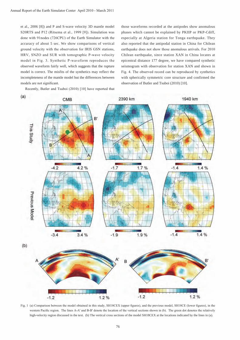
76


et al., 2006 [8]) and P and S-wave velocity 3D mantle model S20RTS and P12 (Ritsema et al., 1999 [9]). Simulation was done with 91nodes (726CPU) of the Earth Simulator with the accuracy of about 5 sec. We show comparisons of vertical ground velocity with the observation for IRIS GSN stations, HRV, SNZO and SUR with tomographic P-wave velocity model in Fig. 3. Synthetic P-waveform reproduces the observed waveform fairly well, which suggests that the rupture model is correct. The misfits of the synthetics may reflect the incompleteness of the mantle model but the differences between models are not significant.

Recently, Butler and Tsuboi (2010) [10] have reported that

those waveforms recorded at the antipodes show anomalous phases which cannot be explained by PKIIP or PKP-Cdiff, especially at Algeria station for Tonga earthquake. They also reported that the antipodal station in China for Chilean earthquake does not show those anomalous arrivals. For 2010 Chilean earthquake, since station XAN in China locates at epicentral distance 177 degree, we have compared synthetic seismogram with observation for station XAN and shown in Fig. 4. The observed record can be reproduced by synthetics with spherically symmetric core structure and confirmed the observation of Butler and Tsuboi (2010) [10].

Fig. 1 (a) Comparison between the model obtained in this study, SH18CEX (upper figures), and the previous model, SH18CE (lower figures), in the western Pacific region. The lines A-A' and B-B' denote the location of the vertical sections shown in (b). The green dot denotes the relatively high-velocity region discussed in the text. (b) The vertical cross sections of the model SH18CEX at the locations indicated by the lines in (a).

77


Fig. 2 (a) The model SH18CEX at the CMB overplotted by the ScS-S residuals previously reported by Takeuchi and Obara (2010). (b) The ScS-S residuals shown in (a), plotted as a function of the azimuth. The azimuth is measured from the centroid of the events analyzed by Takeuchi and Obara (2010) [5] (left). The height of the D'' discontinuity as a function of the azimuth reported by Takeuchi and Obara (2010) [5]. (c) The schematic picture of the structures of the region studied by Takeuchi and Obara (2010) [5]. The red part denotes the chemically distinct region and the solid black lines denote the D'' discontinuity.

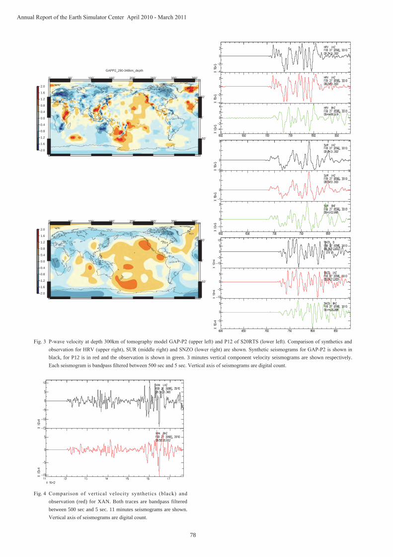
78


Fig. 3 P-wave velocity at depth 300km of tomography model GAP-P2 (upper left) and P12 of S20RTS (lower left). Comparison of synthetics and observation for HRV (upper right), SUR (middle right) and SNZO (lower right) are shown. Synthetic seismograms for GAP-P2 is shown in black, for P12 is in red and the observation is shown in green. 3 minutes vertical component velocity seismograms are shown respectively. Each seismogram is bandpass filtered between 500 sec and 5 sec. Vertical axis of seismograms are digital count.

GAPP2_290-348km_depth

0˚ 50˚ 100˚ 150˚ 200˚ 250˚ 300˚ 350˚

-50˚

0˚

50˚

-2.0

-1.6

-1.2

-0.8

-0.4

0.0

0.4

0.8

1.2

1.6

2.0

0˚ 50˚ 100˚ 150˚ 200˚ 250˚ 300˚ 350˚

-50˚

0˚

50˚

-2.0

-1.6

-1.2

-0.8

-0.4

0.0

0.4

0.8

1.2

1.6

2.0

Fig. 4 Comparison of vertical velocity synthetics (black) and observation (red) for XAN. Both traces are bandpass filtered between 500 sec and 5 sec. 11 minutes seismograms are shown. Vertical axis of seismograms are digital count.

79


References[1] Takeuchi, N., 2007. Whole mantle SH velocity model

constrained by waveform inversion based on three-dimensional Born kernels, Geophys. J. Int., 169, 1153-1163.

[2] Ritsema, J., Deuss, A., van Heijst, H. J., Woodhouse, J. H., 2011. S40RTS: a degree-40 shear-velocity model for the mantle from new Rayleigh wave dispersion, teleseismic traveltime and normal-mode splitting function measurements, Geophys. J. Int., 184, 1223-1236.

[3] Ni, S., Helmberger, D. V., 2003. Seismological constraints on the South African superplume; could be the oldest distinct structure on earth, Earth Planet. Sci. Lett., 206, 119-131.

[4] Wang, Y., Wen, L., 2007. Geometry and P and S velocity structure of the "African Anomaly", J. Geophys. Res., 112, B05313, doi:10.1029/2006JB004483.

[5] Takeuchi, N., Obara, K., 2010. Fine-scale topography of the D'' discontinuity and its correlation to volumetric velocity fluctuations, Phys. Earth Planet. Int., 183, 126-135.

[6] Nakamura, T., Tsuboi, S., Kaneda, Y., Yamanaka, Y., 2010. Rupture process of the 2008 Wenchuan, China earthquake inferred from teleseismic waveform inversion and forward modeling of broadband seismic waves, Tectonophysics, 491, 72-84.

[7] Komatitsch, D., Tromp, J., 2002. Spectral-element simulations of global seismic wave propagation-I. Validation. Geophys. J. Int. 149, 390-412.

[8] Obayashi, M., Sugioka, H., Yoshimitsu, J., Fukao, Y., 2006. High temperature anomalies oceanward of subducting slabs at the 410-km discontinuity, Earth Planet. Science Lett., 243, 149-158.

[9] Ritsema, J., Van Heijst, H. J., Woodhouse, J. H., 1999. Complex shear velocity structure imaged beneath Africa and Iceland. Science, 286, 1925-1928.

[10] Butler, R., Tsuboi, S. , 2010. Antipodal seismic observation of temporal and global variation at Earth's inner-outer core boundary, Geophys. Res. Lett., vol. 37, L11301, doi:10.1029/2010GL042908.

80


全地球弾性応答シミュレーション


坪井　誠司　　海洋研究開発機構　地球内部ダイナミクス領域 /地球情報研究センター

著者坪井　誠司　　海洋研究開発機構　地球内部ダイナミクス領域 /地球情報研究センター竹内　　希　　東京大学　地震研究所

Direct Solution法を用いた波形インバージョンにより、地球内部マントル 3次元地震波速度構造モデルを改善した。これまでより、およそ 3.5倍のデータを用いることにより、より高精度の地球内部構造モデルを得ることが出来た。得られたモデルには、西太平洋下の核マントル境界に局所的な速度異常を示す構造が示されている。スペクトル要素法により現実的な 3次元地球モデルに対する理論地震波形記録を 2010年チリ地震（Mw8.7）に対して

計算した。計算は地球シミュレータの 91ノードを用いて、周期約 5秒の精度で行った。計算した理論地震波形は観測波形をよく説明しており、用いた地震断層モデルがよく断層における破壊過程をモデル化していることを示している。2010年チリ地震に対しては中国大陸の観測点 XANが震央距離 177度と対蹠点に近いところに位置している。XANの理論地震記録は、観測をよく説明しており、計算に用いた球対称内核構造モデルがこの観測点と地震の組み合わせに対しては適用可能であることを示している。

キーワード : 理論地震波形記録 , 3次元地球内部構造 , スペクトル要素法

81


1. IntroductionOur group is composed of two subgroups, aiming for

comprehensive understanding of the dynamics of the Earth's mantle and core as a combined solid-Earth system. The mantle convection group focuses on dynamical behaviors of the Earth's mantle and simulates infinite-Prandtl-number thermal convection. Particular attention has been paid on integrating realistic mantle properties (e.g., variable viscosity, phase transition, plate behaviors) into the model and reproducing the images obtained from seismic tomography. The geodynamo group simulates thermal convection of the fluid outer core and a resultant generation process of the geomagnetic field. In order to reach the core conditions, we have made attempts to reduce viscous effects in the dynamo model by decreasing the Ekman number (E = ν/2Ωr0

2; v: kinematic viscosity, Ω: Earth's angular velocity, r0: core radius), the Prandtl number (Pr = ν/κ ; κ: thermal diffusivity), and the magnetic Prandtl number (Pm = ν/ŋ ; ŋ: magnetic diffusivity). We are also studying the nature of turbulence in liquid metal convection by comparing the results

of numerical simulations with laboratory experiments.

2. Simulations of mantle convectionThe Earth's mantle is composed of solid rocks but it flows

like a viscous fluid in a geologic time scale. This convective flow of the mantle is emerging as the motion of tectonic plates on the Earth's surface. The motion of surface plates causes earthquake, volcanism and mountain building at the plate margins. As the mantle flow transports the heat from the hot interior, the whole of the Earth has been cooling through its history. It also controls the boundary conditions of the outer core. Hence, mantle convection is the key process for understanding the activity and evolution of our planet. Seismic tomography reveals the natural mode of convection in the Earth is whole mantle with subducted plates (slabs) clearly seen as continuous features into the lower mantle. The Earth's mantle is characterized by the coexisting state of slabs stagnating around the transition zone and falling into the lower mantle [1].

We simulated fully dynamical and self-consistent thermal

Simulation Study on the Dynamics of the Mantle and Core in Earth-like Conditions


Yozo Hamano Institute for Research on Earth Evolution, Japan Agency for Marine-Earth Science and Technology

Authors

Takatoshi Yanagisawa*1, Ataru Sakuraba*2, Futoshi Takahashi*3, Yasuko Yamagishi*1 and Yozo Hamano*1

*1 Institute for Research on Earth Evolution, Japan Agency for Marine-Earth Science and Technology

*2 Department of Earth and Planetary Science, School of Science, The University of Tokyo

*3 Department of Earth and Planetary Sciences, School of Science and Engineering, Tokyo Institute of Technology

Thermal convection in the mantle and the outer core is the origins of various Earth's activities and essentially important in the Earth's evolution. We investigated styles of convection in the mantle by using a three-dimensional spherical-shell code that includes effects of phase transitions, temperature-dependent viscosity with plastic yielding near the surface, and viscosity variations in the mantle. We find that, these effects spontaneously reproduce plate-like behaviors and slab stagnation around the transition zone, with appropriate value of viscosity increase in the lower mantle. In the core convection, one of the most important properties is the extremely low viscosity of the fluid. Our high-resolution model for geodynamo successfully simulated torsional oscillations, and we analyzed their details by comparing with theories and observed short-term geomagnetic field variations. On the other hand, we apply a high-order compact difference scheme to treat such thin boundary layers with smaller computational recourses. As a result, faster convergence is achieved and we confirmed the validity of the scheme. In addition, study of turbulence in liquid metal convection is within our scope. Our numerical code on thermal convection with the material properties of a liquid metal can reproduce the character of motion observed by laboratory experiments.

Keywords: mantle convection, slab stagnation, core convection, geodynamo, geomagnetic secular variation, convection of low Prandtl number fluid

82


convection in high-resolution 3-D spherical shell models which range up to Earth-like conditions in Rayleigh number, and succeeded in spontaneous generation of plate-like behavior with slab stagnation [2]. We examined the influence of three factors: phase transitions, temperature dependent viscosity with plastic yielding at shallow depth, and viscosity increase in the lower mantle, and clarified the condition for generating stagnant slabs. The temperature dependent viscosity with plastic yielding spontaneously produces plate-like behavior with very localized convergence zones at the surface. This plate-like structure can stagnate in the transition zone with the combination of 660 km phase transition and viscosity increase in the lower mantle. The model including these three factors with adequate values generates the coexisting state of stagnant and penetrating slabs around the transition zone, which are characteristics of mantle

convection revealed by seismic tomography (Fig. 1). The key mechanism to generate stagnant slabs is the partly decoupled state of the upper and lower mantle flow due to the phase transition. Behaviors of subducted plates are sensitive to the viscosity increase in the lower mantle. We examined several cases by varying the reference viscosity structure through the mantle (Fig. 2). We confirmed that it is necessary more than 40 times of viscosity increase in the lower mantle to form large-scale stagnation. With smaller value of increase, small-scale stagnations are realized, which is different from the views of mantle tomography. If the value of the viscosity increase exceeds 100 times, the behavior of the slab is weakly depends on the value. The steepness of the viscosity increase is also important for the behavior of subducted slabs. If the viscosity increase is more gradual, the range of stagnation depth is

Fig. 1 Various styles of subducted slabs in the mantle. (left) Images from mantle tomography by [3] (blue: high velocity, red: low velocity), (center) the location of each cross-section. (right) Similar styles of subduction reproduced in our 3-D spherical shell convection model containing phase transitions, viscosity layering, and plastic yielding near the surface (blue: low temperature, red: high temperature). The Earth's mantle is characterized by the coexisting states of stagnant and falling slabs, and our numerical model spontaneously reproduces these features.

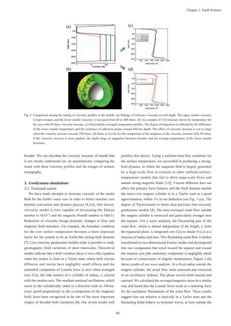
83


broader. We can elucidate the viscosity structure of mantle that is not clearly understood yet, by quantitatively comparing the result with these viscosity profiles and the images of seismic tomography.

3. Geodynamo simulations3.1. Torsional waves

We have made attempts to decrease viscosity of the model fluid for the Earth's outer core in order to better simulate core thermal convection and dynamo process [4,5,6]. Our lowest-viscosity model is now capable of decreasing the Ekman number to O(10-7) and the magnetic Prandtl number to O(0.1). Reduction of viscosity brings dramatic changes to flow and magnetic field structures. For example, the boundary condition for the core surface temperature becomes a more important factor for the system to be an Earth-like strong-field dynamo [7]. Low-viscosity geodynamo models make it possible to study geomagnetic field variations of short timescales. Theoretical studies indicate that a field variation obeys a wave-like equation when the system is close to a Taylor state, where both viscous diffusion and inertia have negligibly small effects and the azimuthal component of Lorentz force is zero when averaged over C(s), the side surface of a cylinder of radius, s, coaxial with the rotation axis. The resultant torsional oscillations, which travel in the cylindrically radial (s-) direction with an Alfven-wave speed proportional to the s-component of the magnetic field, have been recognized to be one of the most important origins of decadal field variations [8]. Our recent model well

justifies this theory. Using a uniform-heat-flux condition for the surface temperature, we succeeded in producing a strong-field dynamo, in which the magnetic field is largely generated by a large-scale flow in contrast to other uniform-surface-temperature models that fail to drive large-scale flows and sustain strong magnetic fields [5,9]. Viscous diffusion does not affect the primary force balance and the fluid domain outside the inner-core tangent cylinder is in a Taylor state to a good approximation; within 1% in our definition (see Fig. 3 (a)). The degree of Taylorization is better than previous low-viscosity geodynamo models [4]. The time-averaged zonal flow outside the tangent cylinder is westward and particularly stronger near the equator. For a wave analysis, the fluctuating part of the zonal flow, which is almost independent of the height, z, from the equatorial plane, is integrated over C(s) to obtain V (s,t) as a function of radius and time. This fluctuating zonal flow is further transformed to two-dimensional Fourier modes and decomposed into two components that travel toward the equator and toward the rotation axis (the stationary component is negligibly small because of conservation of angular momentum). Figure 3 (b) shows results of our wave analysis. At a fixed radius outside the tangent cylinder, the zonal flow turns eastward and westward in an oscillatory fashion. The phase travels both inward and outward. We calculated the averaged magnetic stress in a similar way and found that the Lorentz force acted as a restoring force for the oscillatory fluctuations of the zonal flow. These results suggest that our solution is basically in a Taylor state and the fluctuating fields behave as torsional waves, at least outside the

Fig. 2 Comparison among the setting of viscosity profiles in the mantle. (a) Settings of reference viscosity at each depth. The upper mantle viscosity is kept constant, and the lower mantle viscosity is increased from 40 to 400 times. (b) An example of 3-D structure shown by temperature for the case with 40 times viscosity increase. (c) Horizontally averaged temperature profiles. The degree of stagnation is reflected by the difference of the lower mantle temperature and the existence of inflection points around 660 km depth. The effect of viscosity increase is not so large when the viscosity increase exceeds 100 times. (d) Same as (c) but for the comparison of the steepness of the viscosity increase with 40 times. If the viscosity increase is more gradual, the depth range of stagnation becomes broader and the average temperature of the lower mantle increases.

84


tangent cylinder, as predicted by previous theory.Gillet and coauthors recently reported that the observed

geomagnetic data suggested faster propagation of torsional waves than previously estimated and its cause could be attributed to a stronger interior magnetic field [10]. They also showed that the propagation direction was primarily outward, which is totally different to our calculation. Although a direct comparison to the Earth's core convection is too premature, our solution seems to be still crude to represent ideal torsional waves. For example, there is a trend of slower outgoing propagation in the zonal flow at around t = 1.491 and s = 0.7. This signature cannot be explained by Alfven waves and is probably caused by a local effect of advection. In our model, the magnetic energy density is only ten times greater than the kinetic energy density on average, whereas this ratio, considered to be an index of magnetically dominated strong-field dynamo, is expected to be at least several hundreds in the Earth's core. Simulations of higher-resolution and lower-viscosity geodynamo models are still needed to reach the core condition and to make a comparison to the geomagnetic data.

3.2. Implementation of a high-order scheme

As noted in the previous section, the currently most advanced models are run at E = O(10-7). At such a low-Ekman number, a very sharp Ekman boundary layer with radial thickness of O(E1/2) develops near the inner and outer boundaries of the core. Numerical models must be capable of resolving such thin boundary layers. Since a spectral approach using Chebyshev expansion is, in general, not very good at representing a very sharp structure, we have investigated finite difference discretization for low-Ekman-number simulations. However, in ordinary finite difference discretization, fine mesh and many stencils are needed to yield solutions of acceptable accuracy.

As a result, a lot of memory space and computing time may be consumed. One approach to perform numerical dynamo simulations at a low-Ekman number with high accuracy and less computational cost is to use higher order discretization scheme, which use coarser mesh to yield solutions of comparable

Fig. 4 Convergence behavior of the solutions with respect to radial resolution Nr: (a) kinetic energy, (b) azimuthal velocity, (c) magnetic energy, (d) axial magnetic field, (e) temperature, and (f) drift rate. The present results are classified by L31 and L47 corresponding to spherical harmonic expansion up to 31 and 47, respectively, while ACD, GJZ and TMH denote results from different codes. Horizontal solid lines show the standard values and horizontal dashed lines represent the deviation by 0.5% from the standard values.

Fig. 3 (a) A Taylorization factor defined as the ratio of the integral of Fϕ, the azimuthal component of Lorentz force, over C(s), the side surface of an axial cylinder of radius, s, to the integral of the absolute value of Fϕ over the same surface. Time is scaled by a magnetic diffusion time. Broken line represents the inner core radius. (b) Shown are the time variations of the magnetic torque, BsBϕ, and the azimuthal component of velocity, Vϕ, integrated over C(s). Both integrated BsBϕ and Vϕ represent fluctuations from their time averages and have been decomposed into outgoing (left) and ingoing (right) components by Fourier analysis. The actual fluctuation is the sum of these two components.

85


accuracy relative to the lower order discretization scheme using finer mesh. A combined compact difference scheme (CCDS) can achieve a high-order accuracy and good spectral resolution with a small stencil. We apply a high-order three-point CCDS in the radial direction to problems of thermal convection and convection-driven dynamo in a rotating spherical shell [11]. To evaluate accuracy of the CCDS, we have solved the benchmark problems. It is confirmed that accuracy better than 1% is achieved with the CCDS even with a modest number of grid mesh. Quantitative comparison with other finite difference schemes indicates that the CCDS is superior to others using more stencils. As a result, faster convergence behavior of the CCDS is observed in most quantities with an accuracy of 0.5% (Fig. 4).

3.3. Coherent structure with oscillation in liquid metal

convectionsThe study on the nature of thermal convection in low Prandtl

number fluids is essential for the dynamics of the Earth's outer core, and the difference of the flow behavior from Pr~1 fluids like water and air is very important. In lower Pr fluids, the

two-dimensional steady roll structure emerging at the onset of convective flow easily becomes time-dependent just above the critical Rayleigh number (Ra), and theoretical studies propose oscillatory instability such as "traveling-wave convection" in the direction of the roll axis [12]. Transition to turbulence with increases in Ra in low Pr fluids occurs at much lower Ra than water or air, and large-scale flow is also expected to emerge easily.

Our laboratory experiments on thermal convection with liquid metal by using an ultrasonic velocity profile measurements visualized the flow pattern in a gallium layer with simultaneous measurements of the temperature fluctuations, from 10 to 200 times above the critical Ra [13,14]. It was made in a non-rotating rectangular container. In those experiments, the presence of a roll-like structure with oscillatory behavior was established (Fig. 5), even in the Ra range where the power spectrum of the temperature fluctuation shows features of developed turbulence. The flow structure was interpreted as a continuously developed one from the oscillatory instability of two-dimensional roll convection around the critical Ra. It was shown that both the velocity of the flows and the frequency of

Fig. 5 Setting and result of ultrasonic flow velocity measurements for Rayleigh-Bénard convection in liquid gallium (laboratory experiment). (a) Geometry of the container and setting of the measurement beam lines in liquid gallium. (b) Examples of the velocity profiles for the case Ra = 8x104; horizontal axis is the elapsed time, vertical axis is the position, and color maps indicate the horizontal component of the convective flow velocity. The vertical temperature difference was set at the time = 200 s, and convection pattern emerged after that. Four clusters of velocity with periodic oscillations are clearly observed. (c) Interpretation of the global flow pattern. Oscillatory roll-like structure exists in the vessel, and the oscillation period is comparable to the circulation time of the flow in a roll.

86


the oscillation increase proportional to the square root of Ra, and that the oscillation time of the roll structure is comparable to the time to complete one circulation of the flow.

We made up a code for numerical simulation of thermal convection to compare with the results obtained by the laboratory experiments. Furthermore, we analyzed the fine scale structure and short time variation relating to turbulence, those are difficult to obtain by laboratory experiments due to the limitation of measurements. The numerical simulation is performed for three dimensional rectangular box, with no-slip boundary conditions at all boundaries, fixed temperature at the top and bottom, and insulating at side walls. The range of Ra for numerical simulations is from critical value to 200 times above it. The material properties of the working fluid are those of liquid gallium and Pr=0.025. We used enough grid points to resolve the small-scale behavior without any assumption for the turbulence. Our numerical result reproduced oscillatory convection patterns as observed in the experiments. Statistical values, such as the relation of the circulation time and oscillation period, Rayleigh number dependence of the mean velocity and the oscillation frequency, are good agreement in both laboratory and numerical studies (Fig. 6). This confirms that both of our laboratory experiment and numerical simulation are reliable ones. The series of numerical simulations with the increase in Ra revealed the onset point of oscillatory convection and subsequent transition to turbulence. The power spectrum densities calculated from the velocity and temperature dataset

clearly indicate the feature of low Pr fluid, that is, temperature is more diffusive than momentum and the corner frequency is higher for velocity spectrum in the region of developed turbulence.

References

[1] Y. Fukao, M. Obayashi, T. Nakakuki, and Deep Slab Project Group, "Stagnant slab: A review", Annual. Rev. Earth Planet. Sci., vol.37, pp.19-46, 2009.

[2] T. Yanagisawa, Y. Yamagishi, Y. Hamano, and D. R. Stegman, "Mechanism for generating stagnant slabs in 3-D spherical mantle convection models at Earth-like conditions", Phys. Earth Planet. Inter., vol.183, pp.341-352, 2010.

[3] M. Obayashi, H. Sugioka, J. Yoshimitsu, and Y. Fukao, "High temperature anomalies oceanward of subducting slabs at the 410-km discontinuity", Earth Planet. Sci. Lett., vol.243, pp.149-158, 2006.

[4] F. Takahashi, M. Matsushima, and Y. Honkura, "Simulations of a quasi-Taylor state geomagnetic field including polarity reversals on the Earth Simulator", Science, vol.309, pp.459-461, 2005.

[5] F. Takahashi, M. Matsushima, and Y. Honkura, "Scale variability in convection-driven MHD dynamos at low Ekman number", Phys. Earth Planet. Inter., vol.167, pp.168-178, 2008.

[6] A. Sakuraba and P. H. Roberts, "Generation of a strong

Fig. 6 Quantitative comparison between laboratory experiments and numerical simulations. (a) Velocity profiles by numerical simulations showing Rayleigh number dependence. Oscillatory four-roll structures similar to the laboratory experiments are reproduced. (b) Comparison of non-dimensional flow velocity. (c) Comparison of non-dimensional frequency of the pattern oscillation. These are good agreement between simulations and experiments.

87


magnetic field using uniform heat flux at the surface of the core", Nature Geoscience, vol.2, pp.802-805, 2009.

[7] A. Sakuraba and P.H. Roberts, "On thermal driving of the geodynamo", in The Earth's magnetic interior, E. Petrovsky, E. Herrero-Bervera, T. Harinarayana, and D. Ivers, eds., Springer, 2011 (in press).

[8] R. Holme, "Large-scale flow in the core", in Treatise of Geophysics, Vol.8, P. Olson, ed., pp.107-130, Elsevier, 2007.

[9] A. Kageyama, T. Miyagoshi, and T. Sato, "Formation of current coils in geodynamo simulations", Nature, vol.454, pp.1106-1109, 2008.

[10] N. Gillet, D. Jault, E. Canet, and A. Fournier, "Fast torsional waves and strong magnetic field within the Earth's core", Nature, vol.465, pp.74-77, 2010.

[11] F. Takahashi, "Implementation of a high-order combined compact difference scheme in problems of thermally driven convection and dynamo in rotating spherical shells", Geophys. Astrophys. Fluid Dyn., doi:10.1080/03091929.2011.565337 (in press), 2011.

[12] F. H. Busse, "The oscillatory instability of convection rolls in a low Prandtl number fluid", J. Fluid Mech., vol.52, pp.97-112, 1972.

[13] T. Yanagisawa, Y. Yamagishi, Y. Hamano, Y. Tasaka, M. Yoshida, K. Yano, and Y. Takeda, "Structure of large-scale flows and their oscillation in the thermal convection of liquid gallium", Phys. Rev. E, vol.82, 016320, 2010.

[14] T. Yanagisawa, Y. Yamagishi, Y. Hamano, Y. Tasaka, K. Yano, J. Takahashi, and Y. Takeda, "Detailed investigation of thermal convection in a liquid metal under a horizontal magnetic field: Suppression of oscillatory flow observed by velocity profiles", Phys. Rev. E, vol.82, 056306, 2010.

88


実地球環境でのマントル・コア活動の数値シミュレーション


浜野　洋三　　海洋研究開発機構　地球内部ダイナミクス領域

著者柳澤　孝寿 *1，櫻庭　　中 *2，高橋　太 *3，山岸　保子 *1，浜野　洋三 *1

*1 海洋研究開発機構　地球内部ダイナミクス領域

*2 東京大学　大学院理学系研究科地球惑星科学専攻

*3 東京工業大学　大学院理工学研究科地球惑星科学専攻

地球のマントルとコアで起こっていると考えられる熱対流は、固体地球に生起するさまざまな活動の根本原因であり、地球の進化を知る上で重要である。本プロジェクトではマントルとコアの対流を可能な限り地球に近い条件で取り扱い、実際の現象との比較をおこなってきた。マントルの対流については、すでに開発済みの有限要素法を用いた球殼熱対流コードで実行した。粘性の温度依存性

と表面付近での降伏応力の導入によって、自然にプレート的な運動が再現される条件で、上部マントルと下部マントルの粘性比を等倍から 400倍まで変えて沈み込むプレートの挙動を調べた。結果、粘性比が 40倍を超えると、マントル遷移層でプレートの横たわり（滞留）が顕著に見られるようになった。さらに粘性比を大きくしても横たわりの形態にあまり変化はなく、粘性比そのものよりも粘性増加の勾配が形態に大きく影響することが分かった。代表的なケースについて 30億年以上の時間積分をおこない、プレート配置が長時間にわたって変動し続ける結果を得ることに成功した。本結果を用いて、地震波トモグラフィーで得られた沈み込んだプレートの形状との比較を多くの沈み込み帯についておこなった。コアの対流については、地球ダイナモのシミュレーションを球関数展開とチェビシェフ多項式展開とに基づくスペク

トル変換法を用いた既に開発済みのコードで実行した。結果、低い粘性のもとで理論的に予想されているコアのねじれ振動が、シミュレーションにおいても、内向き・外向きの進行波として存在していることを確認した。さらに、既存モデルで採用していたブシネスク近似から、ゼロでない断熱温度勾配の効果を考慮する近似に変更し、コードの検証をおこなった。同様の離散化を用いたコードで、コア表面に安定成層が存在する条件でのダイナモシミュレーションを比較的粘性の低い領域でおこなった。一方であらたに、動径方向に対する離散化を高次の結合コンパクト差分法で扱うコードを開発し、チューニングをおこなうとともにダイナモベンチマーク問題を解き、手法の有効性を確認した。我々は同時に、コア乱流のモデル化に関する研究を進めており、熱対流の数値シミュレーションでレイリー数を変えたパラメータスタディを液体金属の実際のプラントル数 O (10-2)を用いて実行し、室内実験で得られている大規模流の変動と乱流の特徴を再現することに成功した。

キーワード : マントル対流 , スタグナントスラブ , コア対流 , 地球ダイナモ , 地磁気永年変化 , 低プラントル数の対流

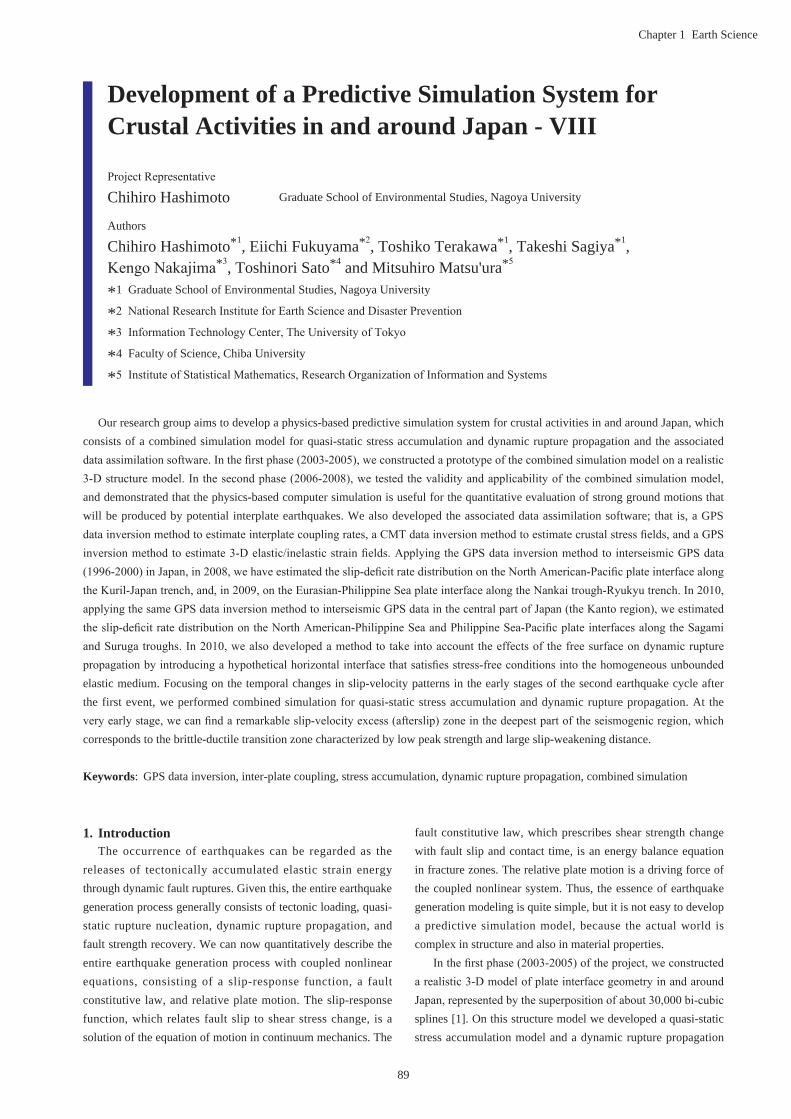
89


1. IntroductionThe occurrence of earthquakes can be regarded as the

releases of tectonically accumulated elastic strain energy through dynamic fault ruptures. Given this, the entire earthquake generation process generally consists of tectonic loading, quasi-static rupture nucleation, dynamic rupture propagation, and fault strength recovery. We can now quantitatively describe the entire earthquake generation process with coupled nonlinear equations, consisting of a slip-response function, a fault constitutive law, and relative plate motion. The slip-response function, which relates fault slip to shear stress change, is a solution of the equation of motion in continuum mechanics. The

fault constitutive law, which prescribes shear strength change with fault slip and contact time, is an energy balance equation in fracture zones. The relative plate motion is a driving force of the coupled nonlinear system. Thus, the essence of earthquake generation modeling is quite simple, but it is not easy to develop a predictive simulation model, because the actual world is complex in structure and also in material properties.

In the first phase (2003-2005) of the project, we constructed a realistic 3-D model of plate interface geometry in and around Japan, represented by the superposition of about 30,000 bi-cubic splines [1]. On this structure model we developed a quasi-static stress accumulation model and a dynamic rupture propagation

Development of a Predictive Simulation System for Crustal Activities in and around Japan - VIII


Chihiro Hashimoto Graduate School of Environmental Studies, Nagoya University

Authors

Chihiro Hashimoto*1, Eiichi Fukuyama*2, Toshiko Terakawa*1, Takeshi Sagiya*1, Kengo Nakajima*3, Toshinori Sato*4 and Mitsuhiro Matsu'ura*5

*1 Graduate School of Environmental Studies, Nagoya University

*2 National Research Institute for Earth Science and Disaster Prevention

*3 Information Technology Center, The University of Tokyo

*4 Faculty of Science, Chiba University

*5 Institute of Statistical Mathematics, Research Organization of Information and Systems

Our research group aims to develop a physics-based predictive simulation system for crustal activities in and around Japan, which consists of a combined simulation model for quasi-static stress accumulation and dynamic rupture propagation and the associated data assimilation software. In the first phase (2003-2005), we constructed a prototype of the combined simulation model on a realistic 3-D structure model. In the second phase (2006-2008), we tested the validity and applicability of the combined simulation model, and demonstrated that the physics-based computer simulation is useful for the quantitative evaluation of strong ground motions that will be produced by potential interplate earthquakes. We also developed the associated data assimilation software; that is, a GPS data inversion method to estimate interplate coupling rates, a CMT data inversion method to estimate crustal stress fields, and a GPS inversion method to estimate 3-D elastic/inelastic strain fields. Applying the GPS data inversion method to interseismic GPS data (1996-2000) in Japan, in 2008, we have estimated the slip-deficit rate distribution on the North American-Pacific plate interface along the Kuril-Japan trench, and, in 2009, on the Eurasian-Philippine Sea plate interface along the Nankai trough-Ryukyu trench. In 2010, applying the same GPS data inversion method to interseismic GPS data in the central part of Japan (the Kanto region), we estimated the slip-deficit rate distribution on the North American-Philippine Sea and Philippine Sea-Pacific plate interfaces along the Sagami and Suruga troughs. In 2010, we also developed a method to take into account the effects of the free surface on dynamic rupture propagation by introducing a hypothetical horizontal interface that satisfies stress-free conditions into the homogeneous unbounded elastic medium. Focusing on the temporal changes in slip-velocity patterns in the early stages of the second earthquake cycle after the first event, we performed combined simulation for quasi-static stress accumulation and dynamic rupture propagation. At the very early stage, we can find a remarkable slip-velocity excess (afterslip) zone in the deepest part of the seismogenic region, which corresponds to the brittle-ductile transition zone characterized by low peak strength and large slip-weakening distance.

Keywords: GPS data inversion, inter-plate coupling, stress accumulation, dynamic rupture propagation, combined simulation

90


model. Then, given the past fault-slip history, we performed the combined simulation of quasi-static stress accumulation and dynamic rupture propagation for the 1968 Tokachi-oki earthquake (Mw=8.2), and demonstrated that when the stress state is close to a critical level, dynamic rupture is rapidly accelerated and develops into a large earthquake, but when the stress state is much lower than the critical level, started rupture is not accelerated [2]. So, the problem is how to know the past fault-slip history and how to monitor the present stress state. In the case of Japan, fortunately, we have nation-wide dense geodetic and seismic observation networks such as GEONET operated by GIS (Geographical Survey Institute of Japan) and F-net operated by NIED (National Research Institute for Earth Science and Disaster Prevention).

In the second phase (2006-2008), we developed the associated data assimilation software; that is, a GPS data inversion method to estimate interplate coupling rates [3], a CMT data inversion method to estimate crustal stress fields [4], and a GPS data inversion method to estimate 3-D elastic/inelastic strain fields [5]. Applying the GPS data inversion method [3] to GEONET data (GSI) in the Hokkaido-Tohoku region for the interseismic calm period of 1996-2000, we estimated the slip-deficit rate distribution on the North American-Pacific plate interface, and revealed that the inverted five slip-deficit peaks almost completely coincide with the source regions of 10 large interplate earthquakes (M>7.5) occurred along the Kuril-Japan trench in the last century [6]. Based on the inversion results, we performed the combined simulation of quasi-static stress accumulation, dynamic rupture propagation and seismic wave propagation for the 2003 Tokachi-oki earthquake (Mw=8.1), and demonstrated that the physics-based computer simulation is useful for the quantitative evaluation of strong ground motions

that will be produced by potential interplate earthquakes [7]. In 2009, applying the GPS data inversion method to interseismic GPS data in the southwestern part of Japan, we estimated the slip-deficit rate distribution on the Eurasian-Philippine Sea plate interface along the Nankai trough-Ryukyu trench, and revealed that a high slip-deficit rate belt extends from the Suruga Bay to the Bungo Channel. On the basis of the inversion results, we computed stress accumulation rates in the seismogenic region, and performed a numerical simulation for the dynamic rupture of a potential Nankai-trough earthquake by using the boundary integral equation method.

2. Interplate slip-deficit rate distribution in and around Japan inverted from GPS data In 2010, applying the GPS data inversion method [3] to

horizontal velocity data at GEONET stations in the central part of Japan for the interseismic calm period of 1996-2000, we estimated precise slip-deficit rate distribution on the North American-Philippine Sea and Philippine Sea-Pacific plate interfaces along the Sagami and Suruga troughs. In the analysis, to remove rigid body translation and block rotation from the observed GPS data, we transform the velocity data into the average strain rates of triangular elements composed of adjacent GPS stations [9]. By this transformation, original information about intrinsic deformation is preserved. Thus, we completed the estimate of interplate coupling rates on the whole plate interfaces in and around Japan. From the slip-deficit rate distribution inverted from GPS data shown in Fig. 1, we can find the high slip-deficit zones along the trench/troughs in the Japan region, corresponding to the past and potential source region of large interplate earthquakes.

Fig. 1 The slip-deficit rate distribution inverted from GPS data ([6,9], Hashimoto, Sagiya & Matsu'ura, SSJ 2009 Fall Meeting). The blue contours indicate the slip-deficit rate.

91


3. Combined simulation for quasi-static stress accumulation and dynamic rupture propagationIn 2010, we also developed a method to take into account

the effects of the free surface on dynamic rupture propagation by introducing a hypothetical horizontal interface that satisfies stress-free conditions into the homogeneous unbounded elastic medium [10]. Applying this method to computation of the dynamic rupture process of the 2008 Iwate-Miyagi earthquake (Mw=6.9), we demonstrated that the effects of the free surface on dynamic rupture propagation is significant in the shallower part of the seismogenic fault.

Now, focusing on the temporal changes in slip-velocity patterns in the early stages of the second earthquake cycle after the first event, we performed combined simulation for quasi-static stress accumulation and dynamic rupture propagation in the 1968 Tokachi-oki seismogenic region [11]. For this computation, we gave the fault slip history in the first earthquake cycle, and then start the quasi-static simulation of tectonic loading for the second earthquake cycle. The panels (a), (b), (c), and (d) in Fig. 2 show the slip-velocity patterns at 1, 2, 3, and 8 yr after the first event, respectively. We can find the slip-velocity deficit zone extending over the source region of the first event at every stage. This indicates the very fast strength recovery in the source region. At the very early stage (a), we can find a remarkable slip-velocity excess (afterslip) zone in the deepest part of the seismogenic region, which corresponds to the brittle-ductile transition zone characterized by low peak strength and large slip-weakening distance. The stress transfer due to viscoelastic relaxation in the asthenosphere may accelerate the afterslip at the depths.

References[1] C. Hashimoto, K. Fukui, and M. Matsu'ura, "3-D

modelling of plate interfaces and numerical simulation of long-term crustal deformation in and around Japan," Pure Appl. Geophys., vol.161, pp.2053-2068, 2004.

[2] M. Matsu'ura, "Quest for predictability of geodynamic processes through computer simulation", Computing in Science & Engineering, vol.7, pp.43-50, 2005.

[3] M. Matsu'ura, A. Noda, and Y. Fukahata, "Geodetic data inversion based on Bayesian formulation with direct and indirect prior information," Geophys. J. Int., vol.171, pp.1342-1351, 2007.

[4] T. Terakawa and M. Matsu'ura, "CMT data inversion using a Bayesian information criterion to estimate seismogenic stress fields," Geophys. J. Int., vol.172, pp.674-685, 2008.

[5] A. Noda and M. Matsu'ura, "Physics-based GPS data inversion to estimate 3-D elastic and inelastic strain fields," Geophys. J. Int., doi:10.1111/j.1365-246X.2010.04611.x, 2010.

[6] C. Hashimoto, A. Noda, T. Sagiya, and M. Matsu'ura, "Interplate seismogenic zones along the Kuril-Japan trench inferred from GPS data inversion," Nature Geoscience, vol.2, pp.141-144, 2009.

[7] E. Fukuyama, R. Ando, C. Hashimoto, S. Aoi, and M. Matsu'ura, "A physics-based simulation of the 2003 Tokachi-oki, Japan, earthquake toward strong ground motion predictions," Bull. Seism. Soc. Am., vol.99, pp.3150-3171, 2009.

[8] T. Yabuki and M. Matsu'ura, "Geodetic data inversion using a Bayesian information criterion for spatial distribution of fault slip," Geophys. J. Int., vol.109, pp.363-375, 1992.

Fig. 2 Temporal changes in slip velocity patterns in the early stages of the second earthquake cycle. The panels (a), (b), (c), and (d) show the slip-velocity patterns at 1, 2, 3, and 8 yr after the first event, respectively. The red and blue contours represent the slip-velocity excess and deficit to steady relative plate motion, respectively. The contour intervals are taken to be 20% of steady relative plate velocities.

92


[9] A. Noda, C. Hashimoto, Y. Fukahata, and M. Matsu'ura, "Inversion of interseismic GPS array data to estimate slip-deficit rates at plate interfaces: Application to the Kanto region, central Japan," Geophys. J. Int., 2011 (submitted).

[10] S. Hok and E. Fukuyama, "A new BIEM for rupture dynamics in half-space and its application to the 2008 Iwate-Miyagi Nairiku earthquake," Geophys. J. Int., vol.184, pp.301-324, 2011.

[11] C. Hashimoto, E. Fukuyama, and M. Matsu'ura, "Physics-based 3-D simulation for the entire process of earthquake generation at plate interfaces in subduction zones," Geophys. J. Int., 2011 (submitted).

93


日本列島域の地殻活動予測シミュレーション・システムの開発 - Ⅷ


橋本　千尋　　名古屋大学　大学院環境学研究科

著者橋本　千尋 *1，福山　英一 *2，寺川　寿子 *1，鷺谷　　威 *1，中島　研吾 *3，佐藤　利典 *4，松浦　充宏 *5

*1 名古屋大学　大学院環境学研究科

*2 防災科学技術研究所　地震研究部

*3 東京大学　情報基盤センター

*4 千葉大学　理学部地球科学科

*5 情報・システム研究機構　統計数理研究所

本研究プロジェクトは、複雑なテクトニック環境の下にある日本列島及びその周辺域を一つのシステムとしてモデル化し、プレート運動に伴う長期的な地殻変形から大地震の発生まで、時間・空間スケールの著しく異なる地殻活動現象を統一的且つ定量的に予測する並列シミュレーション・システムを開発し、モデル計算と観測データを併合した日本列島域の地殻活動予測シミュレーションを行うことを目的としている。地殻活動予測シミュレーション・システムは、日本列島域の 3次元標準構造モデル（CAMP Standard Model; Hashimoto,

Fukui & Matsu'ura, PAGEOPH, 2004）上に構築された、準静的応力蓄積モデル、動的破壊伝播モデル、及び地震／地殻変動データの解析・同化ソフトウェアから成る。平成 20年度には、モデル計算と観測データの融合に向け、直接的及び間接的先験情報を考慮した GPSデータの逆解析手法（Matsu'ura, Noda & Fukahata, GJI, 2007）を北海道－東北地域の地震間（1996-2000）の GPS速度データに適用して北米－太平洋プレート境界の詳細なすべり遅れ分布を求め（Hashimoto, Noda, Sagiya & Matsu'ura, Nature Geoscience, 2009）、その結果に基づいて 2003年十勝沖地震の準静的応力蓄積―動的破壊伝播―地震波動伝播の連成シミュレーションを行ない、将来的に発生が予想されるプレート境界地震による地震動を定量的に予測することが可能なことを示した（Fukuyama et al., BSSA, 2009）。平成 21年度は、上記の GPSデータ逆解析手法を西南日本域に適用してユーラシア－フィリピン海プレート境界の詳細なすべり遅れ分布を明らかにした（Hashimoto, Sagiya & Matsu'ura, SSJ 2009 Fall Meeting）。平成 22年度は、上記の GPSデータ逆解析手法を関東地域に適用して北米－フィリピン海、及びフィリピン海－太平洋プレート境界の固着－すべり状態を推定し（Noda, Hashimoto, Fukahata & Matsu'ura, 2011, GJI, submitted）、昨年度までの結果と合わせて、日本列島全域の震源域のすべり遅れレートの詳細な分布を明らかにした。また、日本列島域の地殻活動予測シミュレーション・システムについては、動的破壊伝播モデルに自由表面の効果を導入する手法を開発し、その効果を評価した（Hok & Fukuyama, GJI, 2011）。更に、1968年十勝沖地震の震源域に於ける，過去の地震による影響を取り込んだ地震発生サイクルシミュレーションにより、地震発生直後に応力蓄積レートが顕著に増大し、やがて時間と共に一定値まで減少すること、また、深部の脆性－延性遷移領域では余効すべりが地震後数年間に亘り継続することが明らかにした（Fukuyama, Hashimoto & Matsu'ura, GJI, submitted）。

キーワード : GPSデータインバージョン , プレート間カップリング , 応力蓄積 , 動的破壊 , 連成シミュレーション

95


1. IntroductionGreat inter-plate earthquakes have occurred at the Nankai

Trough at a recurrence interval of approximately 100 to 150 years due to the subduction of the Philippine Sea plate beneath southwestern Japan (Fig.1).

In the recorded history of the Nankai Trough earthquakes the 1707 Hoei earthquake (hereafter called the Hoei earthquake) was the largest shock in modern Japanese history. It killed more than 20,000 people due to its strong ground motion and the tsunami associated with the earthquake. The fault rupture area of the Hoei earthquake has been thought to spread from Suruga Bay to the westernmost end of Shikoku, which is often referred as a worst-case scenario for the Nankai Trough earthquake.

The source rupture histories of the recent 1944 Tonankai and 1946 Nankai earthquakes were examined extensively based on the analysis of modern instrumental data, such as tide gauge records of tsunami waveforms, seismograms, and geodetic data. However, the source model of the historical Hoei earthquake in 1707, on the other hand, have mostly been deduced from descriptions of earthquake phenomenon in ancient documents such as shaking felt by humans, damage to houses, and visual

measurements of tsunami inundation or tsunami run-up height, and pattern of ground elevation and subsidences.

Recently, geological surveys of earthquake-related lacustrine sediment in seashore lakes along the Pacific coast from Shikoku to Kyushu endeavor to clarify the tsunami history of the historical and pre-historical Nankai Trough earthquakes. Ryujin Lake is one such onshore lake that has tsunami-induced oceanic deposits (hereafter called tsunami lakes), located along the coast of the Hyuga-nada in Kyushu. Ryujin Lake has a thick cover of marine deposits, including coarse-grained sea sands and marine sediments containing oceanic plankton carried by Nankai Trough earthquake, not every 100 to 150 years, but were only deposited in the 1707 Hoei earthquake, the 1361 Shohei earthquake, and the 684 Tenmu earthquakes, probably associated with larger tsunamis than usual. Also, recent findings in the historical documents claim that the height of the tsunami during the Hoei earthquake at the village of Yonouzu, near Ryujin Lake, was more than 10 m, which is very much larger than regular tsunamis associated with the earthquake.

The data from the Japanese GEONET nation-wide GPS network illustrating the current ground deformation pattern of

Tsunami Simulation for the Great 1707 Hoei, Japan, Earthquake using the Earth Simulator


Takashi Furumura Center for Integrated Disaster Information Research, Interfaculty Initiative in Information Studies, The University of Tokyo / Earthquake Research Institute, The University of Tokyo

Authors

Takashi Furumura

Kentaro ImaiTakuto Maeda

Center for Integrated Disaster Information Research, Interfaculty Initiative in Information

Studies, The University of Tokyo / Earthquake Research Institute, The University of Tokyo

Tsunami Engineering Laboratory, Disaster Control Research Center, Tohoku University

Center for Integrated Disaster Information Research, Interfaculty Initiative in Information

Studies, The University of Tokyo / Earthquake Research Institute, The University of Tokyo

The source rupture area of the 1707 Hoei earthquake which occurred along the Nankai Trough, off southwestern Japan, should be extend further, to the Hyuga-nada, more than 70 km beyond the currently accepted location at the westernmost end of Shikoku in order to explain many recent findings such as those for geodetic data and geological investigations in coastal area and large tsunami in Kyushu, Japan. Numerical simulation of the tsunami using a new source-rupture model for the Hoei earthquake explains the distribution of the very high tsunami observed along the Pacific coast from western Shikoku to Kyushu more consistently with tsunami run-up into Ryujin Lake at Kyushu. It is known that the tsunamis from the 684 Tenmu, 1361 Shokei, and 1707 Hoei earthquakes deposited sand in Ryujin Lake, but lesser tsunamis from other earthquakes were unable to reach the lake. This irregular behavior suggests that, in addition to the regular Nankai Trough earthquake cycle of 100-150 years, there may be a hyper-earthquake cycle of 300-500 years. These greater earthquakes produce the larger tsunamis from western Shikoku to Kyushu than we expect for future Nankai Trough earthquake.

Keywords: Earthquake, 1707 Hoei earthquake, Hyuga-nada, Source-rupture model, Tsunami

96


undergoing recovery process of post- Nankai Trough earthquake and studies on inter-plate coupling along the Nankai Trough using this data reveal strong interplate coupling along the Nankai Trough extends to Hyuga-nada.

Following these new findings and supporting instrumental data, we will reexamine the source model for the Hoei earthquake and extended the source-rupture area 70 km eastward to the Hyuga-nada from the westernmost end of Shikoku.

We will demonstrated by tsunami simulation that our new source Hoei earthquake source model can explain large tsunami observed in Kyushu and tsunami inundation into Ryujin Lake more consistently than previous models.

2. Tsunami Simulation for the 1707 Hoei EarthquakeWe first conducted tsunami simulation for the Hoei

earthquake using a source model of An'naka et al. (2003) [1] which consists of four fault segments (N1 to N4) extending from Suruga Bay to the westernmost end of Shikoku, a total length of 605 km.

Vertical ground deformation due to fault rupture of the N1 through N4 fault segments are calculated using the program following Mansinha and Smylie (1975) [2]. The result shows large ground upheavals of up to 2 m above the shallowest end of the source fault segment on the trench side and some of

upheaval can be found on land, including at Cape Muroto, Cape Shiono, and along the coast of Suruga Bay. On the other hand, large surface subsidence of as much as 2 m is found widely on land in a narrow belt zone extending from Shizuoka to the westernmost end of Shikoku. These are consistent with the observed ground deformation pattern of the Hoei earthquake.

Using the results of the coseismic ground deformation pattern, we conducted a tsunami simulation. The area of the simulation is 540 km by 860 km which has been discritized by a nested mesh model that connects gradually 30 m, 90 m, and 270 m mesh model to allow efficient simulation of the tsunami in heterogeneous bathymetry. The bathymetric model was provided by the Central Disaster Mitigation Council, Cabinet Office, Government of Japan. Then propagation of the tsunami and tsunami run-up are calculated based on a finite-difference method (FDM) of a nonlinear, long-wave tsunami model (Goto and Ogawa, 1997) [3].

Snapshots of tsunami propagation obtained from the simulation are illustrated in fig. 2 at time T = 1, 5, 10, 20, 40, and 80 min from the time the earthquake started. The snapshots shows that the radiation of tsunamis from rectangular fault sources is very strong in the direction perpendicular to the trough axis, while it is very weak in the direction parallel to the trough. As the tsunami approaches the shore, its speed decreases suddenly and its height increases very drastically. The onshore height of the tsunami, more than 8 m, is several times larger than the height of the initial tsunami above the source area along the Pacific coast from the westernmost end of Shikoku to Hyuga-nada. The tsunami lasts for several tens of minutes after the earthquake and a number of tsunami trains are captured within Tosa Bay.

Distribution of maximum simulated tsunami height is illustrated in fig. 3. From historical records, tsunami heights of 9 m at Tosa Shimizu and Ashizuri Cape and more than 4 m along the coast from Ashizuri Cape to Hyuga-nada are known to have occurred. The simulated maximum tsunami height along the Pacific coast from Tosa Bay to Suruga Bay generally agrees well with observed tsunami run-up during the Hoei earthquake (e.g., Hatori, 1974 [4], 1985 [5]; Murakami et al., 1996 [6]). However, the height of the simulated tsunami from western Shikoku to Hyuga-nada in Kyushu is less than half of the actual height observed. For example, historical archives document that at Yonouzu village, at the northern end of Hyuga-nada, the tsunami was more than 10 m and killed 18 people (Chida et al, 2003) [7]. Yet the simulated tsunami height at Yonouzu is less than 4 m, much shorter than the tsunami experienced with the Hoei earthquake.

3. Revision of the Source Model for the 1707 Hoei earthquakeIn order to better explain the height of the Hoei earthquake

tsunami from Cape Ashizuri to Hyuga-nada, we revised the

Fig. 1 History of the Nankai Trough earthquake and source rupture area of recent three earthquake sequences of 1944/1946 Showa Tonankai/Nankai, 1854 Ansei, and 1707 Hoei earthquakes.

97


Fig. 2 Snapshots of the tsunami propagation for the 1707 Hoei earthquake at T = 1.0, 5.0, 10.0, 20.0, 40.0, and 80.0 min. Red and blue colors indicate uplift and subsidence of the sea surface, respectively.

Fig. 3 Maximum height of tsunami derive by the tsunami simulation for the former Hoei earthquake source model (black) and new source model (red) comparing with observation (circles).

98


present source model of the Hoei earthquake developed by An'naka et al. (2003) [1] based on the findings of a number of recent geodetic and geological investigations of the Nankai Trough.

Ten years of data from the nationwide GEONET GPS network illustrates pattern of vertical ground deformation of 2 mm/year has occurred on land from Enshu-nada to Hyuga-nada. This pattern of vertical ground movement is considered to illustrate the process of recovery of ground surface deformation due to the Nankai Trough earthquakes. We also consulted recent studies on the spatial distribution of inter-plate coupling rates along the Nankai Trough (e.g., Hashimoto, 2009 [8]) based on the inversion of the GEONET data. It shows that an area of strong inter-plate coupling with high coupling ratios is found from Suruga Bay to Hyuga-nada, more than 100 km beyond the westernmost end of Shikoku which we have considered the evidence that seismic energy is now accumulating to cause a large earthquake in the future.

Following these new findings, we revised the source-rupture model for the Hoei earthquake and extended the border of the Hoei earthquake source segments from the westernmost end of Shikoku to Hyuga-nada, where strong inter-plate coupling has been found.

We set a 70 km by 120 km subfault segment, N5, on the west of the N4 subfault segment and extended the source rupture area of the Hoei earthquake to Hyuga-nada. The ground surface deformation pattern derived using subfaults N1 to N5 agrees well with our expectation of gentle (40 cm) ground subsidence in the area around Yonozu and Ryujin Lake, where large tsunami attacked, and some subsidence of the ground surface at Cape Ashizuri as noted by Kawasumi (1950) [9]. It also corresponds well to the present ground elevation field derived from the GEONET.

We then conducted a tsunami simulation using the revised source model of the Hoei earthquake to see the contribution of the N5 subfault segment in increasing simulated tsunami height along the coast from Shikoku to Kyushu. Snapshots of tsunami propagation are compared in fig. 4 with that for the former source model. Maximum simulated tsunami heights for the new model are compared with those of the former model in fig.3. The comparison clearly demonstrates the development of a larger tsunami with heights of 5 m to over 10 m over a wide area along the Pacific coast from the westernmost end of Shikoku to Hyuga-nada due to the N5 subfault. The height of the tsunami due to the N5 fault is very strong to spread large tsunami wavefront from Cape Ashizuri to Hyuga-nada.

The maximum tsunami height along the coast near Ryujin Lake as calculated by the present simulation is 6 m, while it is a maximum of 2 m for the former Hoei earthquake source model. Thus, larger tsunami at Yonozu and tsunami run-up into Ryujin Lake might occur when the Nankai Trough fault rupture extends to Hyuga-nada, but not during events like the 1854 Ansei

Nankai and 1946 Showa Nankai earthquakes, in which the fault rupture did not extend past the westernmost end of Shikoku. Our newly simulated tsunami height of approximately 6 m but not as high as 10 m at Ryujin Lake also confirms the interpretation of Okamura et al. (2004) [10] that larger tsunami inundation occurred in the Ryujin lake though narrow channel connecting lake and sea but tsunami did not overtopping of beach hills that are 10 m high.

4. ConclusionOf the series of repeating megathrust earthquakes in the

Nankai Trough, the Hoei earthquake is considered to be the most damaging, with its linkage of Tokai, Tonankai and the Nankai earthquakes, and fault ruptures extending from Suruga Bay to the westernmost end of Shikoku, about 600 km in length (An'naka et al., 2003) [1].

However, the recent discovery of the thick cover of tsunami-induced deposits caused by the Hoei earthquake has overturned our understanding. The existence of the tsunami deposits in the onshore lakes in Kyushu was not well explained by the expected ground deformation pattern produced by the former Hoei earthquake source model where the fault rupture stopped at the westernmost end of Shikoku. The source model also failed to explain the larger tsunami experienced during the Hoei earthquake from Cape Ashizuri to Hyuga-nada.

An inferred property of the present crustal deformation pattern illustrated by the GEONET GPS measurements and a number of studies on inter-plate coupling along the Nankai Trough subduction zone based on the GPS data indicate that Hyuga-nada may also be in the area of the Nankai Trough earthquake nucleation zone. Following these new geological and geodetic findings, we revised the source model of the Hoei earthquake by introducing a new subfault segment at Hyuga-nada on the western side of Nankai earthquake segment.

We succeeded in explaining development of the large tsunami from Cape Ashizuri to Hyuga-nada with maximum tsunami heights of 5 to 10 m that attack along the Pacific coast from the westernmost end of Shikoku to Hyuga-nada. This agrees with the heights of tsunamis observed along the Pacific coast from Cape Ashizuri to Hyuga-nada during the Hoei earthquake (Hatori, 1974 [4], 1985 [5]; Murakami, 1996 [6]) very consistently.

The extension of the source rupture area to Hyuga-nada would produce increased shaking in Kyushu. Exactly what the intensity was in Kyushu in 1707 is unclear; we are unaware of any historical documents that permit a meaningful comparison of intensities of the 1707 and 1856 earthquakes.

The linkage process between different subfaults in Nankai Trough earthquakes of more than 700 km and described by at least five fault segments may contribute significantly to the severity of the disaster, especially the tsunamis. Researchers have claimed that delayed rupture between subfaults amplifies

99


tsunami height over a wide area due to overlap of individual tsunamis from different fault segments (Kawata et al., 2003 [11]; Imai et al., 2010 [12]). We should be prepared for a diversity of rupture processes during future earthquakes along the Nankai Trough.

Finally, this study suggests that earthquake rupture extent along the Nankai Trough may not be as limited as previously described: as combinations of subfaults to produce Nankai, Tonankai, or Tokai earthquakes. The Hoei earthquake was a much larger event in which rupture spread as far as Hyuga-nada. Such larger events do not occur during the regular Nankai

Trouh earthquake cycle of 100-150 years, but may occur in a hyper-earthquake cycle of 300 to 500 years. The larger tsunami and tsunami deposits at Ryujin Lake in Kyushu left by large tsunamis from the 684 Tenmu, 1361 Shohei, and 1707 Hoei earthquakes, attest to such a hyper-earthquake cycle.

AcknowledgementsThis study was conducted under support of the Research

Project "Improvements in strong ground motion and tsunami simulation accuracy for application to realistic disaster prevention of Nankai Trough megathrust earthquakes" of the

Fig. 4 Snapshots of tsunami propagation from the Kii Peninsula to Kyushu (a) New Hoei earthquake model with fault segments N1 to N5 (b) former Hoei model (after An'naka et al., 2003 [1]) with fault segments N1 to N4.

100


Ministry of Education, Culture, Sports and Technology of Japan. We thank to the Central Disaster Mitigation Council, Cabinet Office, Government of Japan and Yonouzu Promotion office, Oita Prefecture, Japan to provide bathymetry map data. The results of this study have been published by authors in the Journal of Geophysical Research (vol.116, B02308, doi:10.1029/2010JB007918, 2011) entitled "A revised tsunami source model for the 1707 Hoei earthquake and simulation of tsunami inundation of Ryujin Lake, Kyushu, Japan".

References[1] T. An'naka, K. Inagaki, H. Tanaka, and K. Yanagisawa,

"Characteristics of great earthquakes along the Nankai trough based on numerical tsunami simulation", Journal of Earthquake Engineering, JSCE, CD-ROM, 2003.

[2] L. Mansinha and D. E. Smyli, "The displacement fields of inclined faults", Bull. Seism. Soc. Am., 61, pp.1433-1440, 1971.

[3] C. Goto and Y. Ogawa, "(IUGG/IOC TIME PROJECT), Numerical method of tsunami simulation with the leap-frog scheme, Part 1 Shallow water theory and its difference scheme, Intergovernmental Oceanographic Commission, Manuals and Guides", No.35, 43p., 1997.

[4] T. Hatori, "Sources of large tsunamis in southwest Japan." J. Seismol. Soc. Japan 27, pp.10-24, 1974.

[5] T. Hatori, "Field investigation of Historical tsunamis along the east coast of Kyushu, West Japan", Bull. Earthq. Res. Inst. Univ. Tokyo, 60, pp.439-459, 1985.

[6] H. Murakami, T. Shimada, S. Itoh, N. Yamamoto, and J. Ishizuka, "Reexamination of the heights of the 1606, 1707 and 1854 Nankai Trsunamis along the coast of Shikoku Island", J. SNDS, 15-1, pp.39-52, 1996.

[7] N. Chida, S. Takamiya, H, Hamada, T. Tomimatsu, and S. Mitarai, "Historical materials of the tsunamis in Yonouzu village, southerm part of Oita prefecture, southwest Japan, which were caused by earthquakes of October 28, 1707 and Nobember 24, 1854", Res. Bull. Fac. Educ. & Welf. Sc., Oita Univ, pp.129-143, 2003.

[8] C. Hashimoto, T. Sagiya, and M. Matsuura, "Interplate coupling in southwest Japan inferred from GPS data inversion", Abst. SSJ Meet., pp.A32-08, 2009.

[9] H. Kawasumi, "Crustal deformations as deduced from mareographic data", Publ. Shikoku-Tiho Sogo-Kaihatsu Shingikai (Committee for the Synoptic Development of the Shikoku District), 1950.

[10] M. Okamura, H. Matsuoka, N. Chida, and K. Shimazaki, "Recurrence intervals of super Nankai earthquakes", Abst. Fall Meet. Seism. Soc. Japan, A027, 2004.

[11] Y. Kawata, S. Suzuki, and T. Takahashi, "An effect of giant earthquake scenarios at the Nankai trough on a tsunami hazard", Proceedings of Coastal Engineering, JSCE, 50, pp. 326-330, 2003.

[12] K. Imai, K. Satake, and T. Furumura, "Amplification of tsunami heights by delayed rupture of great earthquakes along the Nankai trough", Earth Planets Space, 62, pp.427-432, 2010.

101


地球シミュレータによる 1707 年宝永地震の津波シミュレーション


古村　孝志　　東京大学　大学院情報学環総合防災情報研究センター

　　　　　　　東京大学　地震研究所

著者古村　孝志　　東京大学　大学院情報学環総合防災情報研究センター　　　　　　　東京大学　地震研究所今井健太郎　　東北大学　大学院工学研究科附属災害制御研究センター前田　拓人　　東京大学　大学院情報学環総合防災情報研究センター　　　　　　　東京大学　地震研究所

近年の地震研究から、南海トラフで発生した 1707年宝永地震の震源域は、これまで想定していた足摺岬までではなく日向灘にかけてさらに 70 km以上延びていた可能性が高くなってきた。このことを受けて、地球シミュレータを用いて宝永地震の新しい震源モデルを用いた津波と強震動シミュレーションを実施した。特に、宝永地震時に大分県佐伯町の龍神池で津波堆積物が保存されていることに着目し、新しい震源モデルによる津波を評価して、さらに津波の浸水シミュレーションを行ってモデルの確かさを検証した。これにより、南海トラフでは 100-150年周期で規則的に大地震が起きているだけでなく、宝永地震のように東海・東南海・南海地震が 3連動発生して震源域が拡大し、四国～九州の津波が高くなる現象が 300-500年に一度起きていたことが明らかとなり、将来の南海トラフ地震による強震動と津波の予測を行う上で新たな課題が提示された。

キーワード : 地震 , 津波 , 1707年宝永地震 , 南海トラフ

103


1. Geodynamo simulation (Miyagoshi)The length-of-day variation of rotation speed is observed

in the Earth. It possibly affects the outer core convection, magnetohydrodynamic dynamo process, and variation of geomagnetic field. Correlation of geomagnetic field variation with length-of-day variation has been pointed out. For example, the relation between geomagnetic field variation and Milankovitch cycle is a controversial issue [1]. The orbital element of the Earth is known to change with Milankovitch cycle. It could causes variation of solar radiation which relates to the cycle between ice age and interglacial age. Prosperity and decline of continental ice sheet may change the mass distribution of water on the earth and its inertial moment. As a result, the rotational speed of the Earth can change.

However, there are no geodynamo models which take an effect of length-of-day variation into consideration. In this fiscal year, we have constructed the first geodynamo model which includes the length-of-day variation effect, based on the Yin-Yang geodynamo dynamo model [2][3]. The points

of the development are as follows. In a momentum equation of magnetohydrodynamic equation, rotation speed in Coriolis force term was uniform. Then, we have added fluctuation of the rotational speed to the Coriolis force term. In addition, a new force term with time differential of rotation speed is newly added to the momentum equation. The length-of-day variation is given by a single frequency sin function with two parameters (amplitude and period of the variation).

As a default, we give the Ekman number, which means the ratio of diffusion force to Coriolis force, as 1.9E-5 (strong rotation) and the Rayleigh number, which means the ratio of buoyancy force to diffusion force, as 1.5E8. Here, both of Prandtl and magnetic Prandtl numbers are unity. First we calculated without rotation speed variation, and found that magnetohydrodynamic dynamo occurred. Then Magnetic energy in the outer core is found to be amplified and saturated several times larger than the kinetic energy. Magnetic dipole moment is also found to be the largest one among other higher moments.

Development of Advanced Simulation Methods for Solid Earth Simulations


Akira Kageyama Graduate School of System Informatics, Kobe University

Authors

Akira Kageyama*1, Mamoru Hyodo*2, Mikito Furuichi*2, Takehiro Miyagoshi*2, Masanori Kameyama*3 and Nobuaki Ohno*4

*1 Graduate School of System Informatics, Kobe University


*3 Geodynamics Research Center, Ehime University

*4 Graduate School of Simulation Studies, University of Hyogo

Geodynamo: We have developed our simulation code of geodynamo to include length-of-day variation effect. By this, we found that the magnetic energy, convection kinetic energy, and magnetic dipole moment oscillate as the Earth's rotation speed changes. The amplitude of magnetic energy oscillation is much larger than that of rotation speed oscillation in the long period (almost the same as magnetic diffusion time) case. The oscillation phase between magnetic and kinetic energy slides pi radian. Numerical planet: We have developed a simulation code of the Stokes flow system with a free surface under a self gravitating field. The largely deformable surface of a planetary body is represented by a distribution of color function. The gravity potential is used for calculating self-gravitating field. A low viscous material (sticky air) surrounding the planet mimics its free surface motion. As an example of our target problem, we have conducted the core formation simulations in three dimensions. Mantle convection: We are also developing a simulation code of mantle convection which includes the effect of two-phase flow, i.e., molten and solid phases. By assuming the motion of the molten phase as a permeable flow through a solid matrix, we successfully solved a fast migration of molten phase even in the presence of slow (Stokes) flow in a solid phase.

Keywords: Geodynamo simulation, Yin-Yang grid, Length-of-Day variation, Mantle convection, Core formation, Stokes flow, mixed precision arithmetic, Two-phase flow, Permeable flow

104


Next, we calculate cases including length-of-day variation effect. For a typical case, we put the period of a variation to be almost equal to the magnetic diffusion time, and the amplitude of a variation to be two percent of the rotation speed. Our simulation results show that the length-of-day variation causes oscillations of magnetic energy, convection kinetic energy, and magnetic dipole moment. These periods are the same as that of rotation speed (magnetic diffusion time). On the other hands, the amplitudes of magnetic energy and magnetic dipole moment oscillation are about one hundred percent, which are quite larger than the amplitude of rotation speed variation (two percent). The amplitude of kinetic energy oscillation is about fifty percent. It is found that the oscillation phase between magnetic and kinetic energy slides pi radian.

We also calculate the case with short period which is one percent of magnetic diffusion time. Different from the long period case, the kinetic energy of convection oscillates rapidly with large amplitude (about one hundred percent), but magnetic energy does not. Magnetic dipole moment oscillates with the same period with the amplitude about several percent.

In the next fiscal year, we would like to search the dependence of oscillation on various rotational frequency and amplitude, and Ekman number, Rayleigh number, and so on.

Especially, we would like to study the case, in which rotational speed varies with several frequencies (not one frequency).

2. Development of numerical planet simulation code (Furuichi)The simulation of the Stokes flow system is an interesting

challenge in the field of computational geodynamics because it is relevant to the numerical study of the mantle dynamics that plays an essential role in the Earth's long-time scale thermal evolution. In this FY, we have developed a new solution code of the Stokes flow, which deals with a motion of free surface under a self-gravitation (Fig. 1) on ES2. Our code aims to simulate the long-time scale evolution of solid earth system with realistic boundary (surface) conditions, and is a part of NEMS (Numerical Earth Model Suites) project.

For the numerical treatment of free surface and self-gravitation, we employ a 'spherical Cartesian' approach, in which the surface of the deformable planetary body is defined by the color functions in the Cartesian geometry. In addition, a sticky air, which has very small viscosity with zero density, is introduced around the planetary object to mimic the free surface of the planet. As for a transport of color function, we use the CIP-CSLR method, which is the low diffusive advection

Fig. 1 Snapshot of the simulated evolution of two layered system with free surface in self-gravitating field (a) initial state; (b) intermediate state; (c) steady state layered sphere. Outer half cropped isovolume and inner white isosurface represent color function of s = 1 and s = 2 respectively. Two layer have the same isoviscous property and density, surrounded by the sticky air.

(a) (b) (c)

Fig. 2 Snapshots of the core formation simulation with three layered model in soft core scenario (a) initial state; (b) intermediate RT instability mode; (c) resultant layered sphere. Outer most semi-transparent isosurface and half cropped white isosurface represent mass density at ρ = 0.2 , and color function at Φ2 = 0.8 respectively. The color on ortho plane shows mass density. Property of each layer are given by (ƞair =10-3, ρair = 0.0), (ƞ1 =100, ρ1 = 0.83), (ƞ2 = 10-3, ρ2 = 1.67) and (ƞ3 =10-3, ρ3 = 1.0).

(a) (b) (c)

105


method based on a fully fixed Eulerian mesh and suitable for a computation on the vector processors [4-5]. Self-gravitation is obtained by solving the Poisson equation of gravity potential. The ill-conditioned Stokes flow problems due to sticky air and rheological modeling are solved by the preconditioned Krylov subspace method in a fully coupled approach of the velocity-pressure system. By using a strong Schur complement preconditioner with mixed precision arithmetic utilizing the double-double method [6-7], our newly developed solver is robust to the large viscosity jump. In order to get scalability against an increasing problem size, our iterative Stokes flow solver also involves the Geometric multigrid (GMG) process as preconditioner, and its computational cost is dominant in the overall performance of the solver. Therefore, in order to achieve efficient parallel performance on ES2, careful implementation of GMG method with agglomeration technique is required [7].

Our simulation could successfully reproduce the evolution of Rayleigh-Taylor instability of spherical metal layer (Fig. 1) with various model parameters. This simulation code allows one to tackle the controversial issue of the overturn process in the Earth's core formation, between the central planetary embryo and surrounding iron layer (Fig. 2).

3. Development of mantle convection simulation code (Kameyama)In this project, we are also developing a new simulation

code of mantle convection, based on our own code named "ACuTEMan" [8-10], which includes the effect of two-phase flow, i.e., the presence and/or migration of molten materials in a solid mantle. Through the temporal evolution of the terrestrial planets, two-phase flow is considered to play crucial roles in the development of thermal and chemical structures of the interior by, for example, an intrusion of molten liquid iron into an unmolten (silicate) protocore in the earliest stage of the planets. Therefore, it is one of the most important directions of the studies of solid Earth sciences to establish numerical techniques of large-scale simulations of mantle convection incorporating the effects of two-phase flow.

In this FY, we concentrated our effort to the construction of the numerical techniques of material transport in two-phase system. In particular, we focused on an efficient scheme of motion of molten (liquid) phase, which is expected to occur much faster than that of highly viscous (solid) phase. Here, we assumed that the motion of the liquid phase takes place as a permeable flow through a solid matrix. Note that the validity of the above technique in solid Earth sciences has been already demonstrated by one-dimensional numerical modeling of fluid migration during a shear deformation of fault zone [11]. In addition, we extended the technique to the problems where a flow occurs simultaneously in both the molten (liquid) and unmolten (solid) phases, by assuming that the motion of solid phase is driven by the balance between the viscous resistance

and the buoyancy force coming from the mixture of two phases. By conducting several preliminary calculations with varying permeability and/or density gap between the phases, we have confirmed that our numerical technique successfully solve the motion of molten phase even in the presence of flow in solid phase.

References [1] Yozo Hamano, (In Japanese) Kagaku, vol. 62, No. 1, pp.

14-18, 1992.[2] Akira Kageyama, Takehiro Miyagoshi, and Tetsuya Sato,

Formation of current coils in geodynamo simulations, Nature, vol. 454, pp. 1106-1109, 2008.

[3] Takehiro Miyagoshi, Akira Kageyama, and Tetsuya Sato, Zonal flow formation in the Earth's core, Nature, vol. 463, pp. 793-796, 2010.

[4] M. Furuichi, M. Kameyama, and A. Kageyama, Three-Dimensional Eulerian method for large deformation of viscoelastic fluid: Toward plate-mantle simulation, J. Comput. Phys. vol. 227, pp. 4977-4997, 2008.

[5] M. Furuichi, M. Kameyama, and A. Kageyama, Validity test of a Stokes flow solver by fluid rope coiling: toward plate-mantle simulation, Phys. Earth Planet. Interiors, vol. 176, pp. 44-53, 2009.

[6] M. Furuichi, D. A. May, and P. J. Tackley, Development of a Stokes Flow Solver Robust to Large Viscosity Jump Using a Schur Complement Approach with Mixed Precision Arithmetic, J. Comput. Phys (submitted).

[7] M. Furuichi, Numerical modeling of three dimensional self-gravitating Stokes flow problem with free surface, Procedia Computer Science, 4, 1506-1515, 2011.

[8] Scott D. King, Changyeol Lee, Peter E. van Keken, Wei Leng, Shijie Zhong, Eh Tan, Nicola Tosi, and Masanori Kameyama, A Community Benchmark for 2D Cartesian Compressible Convection in the Earth's Mantle, Geophys. J. Int., vol. 180, pp. 73-87, 2010.

[9] Masanori Kameyama, Akira Kageyama, and Tetsuya Sato, Multigrid iterative algorithm using pseudo-compressibility for three-dimensional mantle convection with strongly variable viscosity, J. Comput. Phys., vol. 206, pp. 162-181, 2005.

[10] ACuTEMan: A multigrid-based mantle convection simulation code and its optimization to the Earth Simulator, J. Earth Simulator, vol. 4, pp. 2-10, 2005.

[11] Kohtaro Ujiie, Masanori Kameyama, and Asuka Yamaguchi, Geological record of thermal pressurization and earthquake instability of subduction thrusts, Tectonophysics, vol. 485, pp. 260-268, 2010.

106


先端的固体地球科学シミュレーションコードの開発


陰山　　聡　　神戸大学　大学院システム情報学研究科

著者陰山　　聡 *1，兵藤　　守 *2，古市　幹人 *2，宮腰　剛広 *2，亀山　真典 *3，大野　暢亮 *4

*1 神戸大学　大学院システム情報学研究科


*3 愛媛大学　地球深部ダイナミクス研究センター

*4 兵庫県立大学　大学院シミュレーション学研究科

我々は、地球ダイナモやマントル対流をはじめとする地球内部のダイナミクスの全体像を理解するために、地球シミュレータを駆使した大規模計算機シミュレーション研究を行っている。そして、そのために必要となる大規模並列計算手法や基本数値アルゴリズムの独自開発に積極的に取り組んでいる。ダイナモ：地球自転速度変動の効果を考慮した地球ダイナモシミュレーションコードを開発した。典型ケースとして

自転速度が磁場散逸時間の周期で変動する場合、磁気エネルギー、磁場ダイポール成分共に約 2倍の振動が生じた。これは自転速度変動の振幅（自転速度の 2％）よりもはるかに大きかった。外核の磁気エネルギーと運動エネルギーは丁度 180度逆位相で変動した。数値惑星：本年度は、自己重力下での自由境界表面をともなうストークス流れを解くシミュレーションコードを開発

した。そして、地球の中心核（コア）の形成過程を 3次元において再現することに成功した。マントル：固体マントル中で溶融相（液相）の運動を取り扱う手法の開発を行った。予備的な計算の結果、開発した

手法は固相のストークス流と液相の浸透流の双方を同時に、かつ適切に取り扱いできることを確認した。

キーワード : 地球ダイナモ , インヤン格子 , 地球回転変動 , マントル対流 , 非弾性流体近似 , コア形成 , ストークス流れ , 2相流 , 浸透流

107


1. IntroductionDuring explosive volcanic eruptions, a mixture of hot ash

(pyroclasts) and volcanic gas is released from the vent into the atmosphere. The mixture generally has an initial density several times larger than atmospheric density at the volcanic vent. As the ejected material entrains ambient air, the density of the mixture decreases because the entrained air expands by heating from the pyroclasts. If the density of the mixture becomes less than the atmospheric density before the eruption cloud loses its upward momentum, a buoyant plume rises to form a plinian eruption column. On the other hand, if the mixture loses its upward momentum before it becomes buoyant, the eruption column collapses to generate a pyroclastic flow. Because the impact and type of volcanic hazards are largely different between these two eruption regimes, the prediction of the condition where an eruption column collapses to generate a pyroclastic flow has been of serious concern; we refer to this condition as "the column collapse condition" [e.g., 1].

Previously, the 1-dimensional (1-D) steady eruption column models [e.g., 2] enabled us to predict column heights and column collapse condition for given magma properties (e.g., water content, ng0, and temperature, T0) and source conditions (e.g., vent radius, L0, velocity, w0, and mass discharge rate, m0). These models capture the basic physics of column collapse, and their predictions show a quasi-quantitative agreement with field observations of witnessed eruptions [e.g., 3]. Recent works based on the numerical simulations [4] pointed out that

the column collapse condition depends on the 2-D and 3-D structures of flow. The flow of a gas-pyroclast mixture near the vent is characterized by a concentric structure consisting of an outer shear region and inner dense core. When the mixture is ejected from a large vent, the outer shear region cannot reach the central axis before the initial momentum is exhausted, so that the inner dense core generates a fountain structure. On the other hand, for the eruption from a relatively narrow vent, the inner dense core disperses due to turbulent mixing and the eruption cloud collapses without a fountain structure.

In this study, we attempt to systematically understand how these 2-D and 3-D effects modify the column collapse condition. For this purpose, we carried out a number of 3-D numerical simulations of eruption cloud with a high spatial resolution. On the basis of an extensive parameter study, we made regime maps of different flow patterns and determined the column collapse condition.

2. Model DescriptionThe simulations are designed to describe the injection of a

gas-pyroclasts mixture from a circular vent above a flat surface in a stationary atmosphere with a temperature gradient typical of the mid-latitude atmosphere. The vent is located in the center of the ground surface. The physical domain involves a vertical and horizontal extent of a few kilometers to several tens of kilometers. At the ground boundary, the free-slip condition is assumed for the velocities of the ejected material and air. At the

3-D Numerical Simulations of Volcanic Eruption Column Collapse


Takehiro Koyaguchi Earthquake Research Institute, The University of Tokyo

Authors

Yujiro SuzukiTakehiro Koyaguchi

Earthquake Research Institute, The University of TokyoEarthquake Research Institute, The University of Tokyo

During an explosive volcanic eruption, an eruption cloud forms a buoyant eruption column or a pyroclastic flow. We investigated the critical condition that separates these two eruption styles (column collapse condition) by performing a series of three-dimensional numerical simulations. We identified two types of column collapse in the simulations: collapse from a turbulent jet which efficiently entrains ambient air (jet-type collapse) and that from a fountain with a high concentration of ejected materials (fountain-type collapse). Which type of collapse occurs depends on whether the critical mass discharge rate for column collapse (MDRC) is larger or smaller than that for the generation of fountain (MDRF) for a given exit velocity. When the magma temperature is relatively low, MDRC is smaller than MDRF; therefore, the jet-type column collapse occurs at the transition between a buoyant eruption column and a column collapse. When the magma temperature is high, on the other hand, MDRC is larger than MDRF; the column collapse always occurs in the fountain-type regime.

Keywords: volcanic eruption cloud, column collapse condition, pseudo-gas model, turbulent mixing, volcanic hazard

108


upper and other boundaries of computational domain, the fluxes of mass, momentum, and energy are assumed to be continuous. A gas-pyroclasts mixture with fixed temperature and water content is assumed to erupt at a constant velocity and mass discharge rate at the vent. We assume that the pressure at the vent is same as the atmospheric pressure for simplicity.

We apply a pseudo-gas model; we ignore the separation of solid pyroclasts from the eruption cloud and treat an eruption cloud as a single gas whose density is calculated from mixing ratio of the ejected material and entrained air. The fluid dynamics model solves a set of partial differential equations describing the conservation of mass, momentum, and energy, and constitutive equations describing the thermodynamic state of the mixture of pyroclasts, volcanic gas, and air. These equations are solved numerically by a general scheme for compressible flow. In this study, the calculations are performed on a 3-D domain with a non-uniform grid. The grid size is set to be sufficiently smaller than L0/8 near the vent. Details of the numerical procedures used in this study are described in Suzuki et al. [4].

3. Flow Patterns of Eruption CloudIn order to capture the characteristics of flow patterns and to

determine the column collapse condition, we have performed a parameter study involving about 100 numerical simulations for variable temperature (T0=550, 800, and 1000 K) and water content (ng0=0.0123 and 0.0284). The mass discharge rate ranges from 104 to 109 kg s-1. The exit velocity is set to be 0.5a - 3a, where a is the sound velocity of gas-pyroclasts mixture.

The flow patterns in the simulation results are classified into four flow regimes: eruption column with jet structure, eruption column with fountain structure, jet collapse, and fountain collapse. The representative features of each flow regime are described below.

When the mixture is ejected from a narrow vent (L0=49 m, T0=1000 K), a stable eruption column develops (Figs. 1a and 1b). The gas-pyroclasts mixuture is ejected from the vent as a dense, high speed jet. After traveling a short distance from the vent, the flow at the boundary between the jet and the ambient air becomes unstable. The jet entrains ambient air by this shear instability: it forms an annular mixing layer which surrounds an unmixed core flow (Fig. 1a). We refer to the mixing layer and the unmixed core flow as "the outer shear layer" and "the inner flow", respectively. The inner flow is eroded by the outer shear layer and disappears at a certain level. As the eruption column further ascends, the flow becomes highly unstable and undergoes a meandering instability that induces efficient mixing. This stream-wise growth of the instabilities results in a complex density distribution in the eruption cloud. Near the vent, the outer shear layer has a lower density than that of air owing to expansion of entrained air, whereas the inner flow remains denser than air (Fig. 1b). After mixing by the meandering

instability, the mixture of the ejected material and the entrained air generates a buoyant column. We refer to this flow regime as "the jet-type column".

When the gas-pyroclast mixture is ejected from a large vent (L0=154 m, T0=1000 K), the fountain structure develops (Figs. 1c and 1d). Just above the vent, the inner flow is eroded by the outer shear layer (Fig. 1c). In this run, because the vent radius is large, the inner flow reaches the height where the initial momentum is exhausted before the boundary between the inner flow and outer shear layer meets the axis of the flow. The ejected material in the inner flow subsequently spreads radially at this height because of the larger density than that of air (Fig. 1d). Such radially suspended flow is commonly observed in a fountain which results from the injection of a dense fluid upwards into a fluid of lower density. The ejected material is intensively mixed with the ambient air by the large-scale eddy of the radially suspended flow. After the entrainment of ambient air, the resultant mixture becomes buoyant and generates upward flows from the large-scale eddy. We refer to this flow regime as "the fountain-type column".

When the gas-pyroclast mixture is ejected from an extremely large vent (L0=403 m, T0=1000 K), the eruption column collapses from a fountain (Figs. 1e and 1f). As the vent radius increases, the ratio of the entrained air against the ejected material decreases, so that the average density of the mixture increases. In this run, the dense part of the ejected material in the fountain collapses to generate pyroclastic flows (Fig. 1f). We refer to this flow regime as "the fountain-type collapse".

In contrast to the fountain-type collapse, when a low-temperature mixture is ejected from a narrow vent (L0=11 m, T0=550 K), the eruption column collapses from a jet (Figs. 1g and 1h). In this run, the jet entrains ambient air by the shear instability; the inner flow disappears at a height of 0.5 km (Fig. 1g). The mixture of the ejected material and the entrained air continues rising up to ~1.0 km and falls down to generate a pyroclastic flow because it has a larger density than that of air (Fig. 1f). As the temperature of the ejected material is lower, the larger amount of air should be entrained for eruption cloud to become buoyant. In this run, the eruption cloud remains heavier than air even though it entrains a large amount of air. We refer to this flow regime as "the jet-type collapse".

4. Flow Regime MapsOn the basis of the parameter studies, we made new flow

regime maps (Fig. 2). When the magma temperature is relatively low (T0=550 K), three flow regimes are identified: the jet-type column, the jet-type collapse, and the fountain-type collapse regimes (Fig. 2a). When the magma temperature is high (T0=1000 K), on the other hand, the possible flow regimes are the jet-type column, the fountain-type column, and the fountain-type collapse regimes (Fig. 2b).

The variation in the flow regime map suggests that two

109


Fig. 1 Numerical results of the gas-pyroclasts mixture ejected from the volcanic vent. Figures (a), (c), (e) and (g) illustrate the cross-sectional distributions of the mass fraction of the ejected material in x - z space. Figures (b), (d), (f) and (h) illustrate the cross-sectional distributions of the density difference relative to the stratified atmospheric density at the same vertical position, -Δρ/ρa=1- ρ/ρa, in x - z space. (a, b) The jet-type column at 600 s after the beginning of the eruption (m0=1x107 kg s-1, L0=49 m, w0=173 m s-1, T0=1000 K, ng0=0.0284). (c, d) The fountain-type column at 190 s (m0=1x108 kg s-1, L0=154 m, w0=173 m s-1, T0=1000 K, ng0=0.0284). (e, f) The fountain-type collapse at 500 s (m0=1x109 kg s-1, L0=403 m, w0=254 m s-1, T0=1000 K, ng0=0.0284). (g, h) The jet-type collapse at 120 s (m0=1x106 kg s-1, L0=11 m, w0=179 m s-1, T0=550 K, ng0=0.0284).

0 3-3x [km]

03

z [k

m]

(a) T0=1000 K L0=49 m

0 3-3x [km]

03

z [k

m]

0 3-3x [km]

03

z [k

m]

0 3-3x [km]

03

z [k

m]

0 0.5-0.5x [km]

00.

5z

[km

]

0 0.5-0.5x [km]

00.

5z

[km

]

01

0.5

0 10-10x [km]

010

z [k

m]

-0.5

0.5

0

0 10-10x [km]

010

z [k

m]

01

0.5

01

0.5

01

0.5

-0.5

0.5

0-0

.50.

50

-0.5

0.5

0

(b) T0=1000 K L0=49 m

(d) T0=1000 K L0=154 m

(c) T0=1000 K L0=154 m

(g) T0=550 K L0=11 m

(h) T0=550 K L0=11 m

(e) T0=1000 K L0=403 m

(f) T0=1000 K L0=403 m

Mass fraction of magma Density difference

110


critical conditions control the transition of the flow regimes: the column collapse condition (solid curves) and the critical condition for the generation of fountain (dashed curves). When the temperature is relatively low, the critical mass discharge rate for the column collapse (MDRC) is smaller than that for the generation of fountain (MDRF) for a given exit velocity (Fig. 2a). In this case, the column collapse occurs in the jet-type and fountain-type regimes. The flow pattern at the column collapse condition is characterized by the jet-type collapse. As the exit velocity increases, MDRC increases with a slope similar to that predicted by the 1-D model (see solid and dotted curves in Fig. 2a). When the temperature is high, on the other hand, MDRC is larger than MDRF. In this case, the column collapse always occurs in the fountain-type regime (Fig. 2b). The column collapse condition for the fountain-type regime is largely different from that predicted by the 1-D model; the increase rate of MDRC based on the 3-D simulations is larger than that based on the 1-D model (see solid and dotted curves in Fig. 2b).

References[1] R. S. J. Sparks and L. Wilson, "A model for the formation

of ignimbrite by gravitational column collapse", J. Geol. Soc. Lond., 132, 441-451, 1976.

[2] A. W. Woods, "The dynamics of explosive volcanic eruptions", Rev. Geophys., 33(4), 495-530, 1995.

[3] S. Carey, H. Sigurdsson, J. E. Gardner, and W. Criswell, "Variations in column height and magma discharge during the May 18, 1980 eruption of Mount St. Helens", J. Volcanol. Geotherm. Res., 43, 99-112, 1990.

[4] Y. J. Suzuki, T. Koyaguchi, M. Ogawa, and I. Hachisu, "A numerical study of turbulent mixing in eruption clouds using a three-dimensional fluid dynamics model", J. Geophys. Res., 110, B08201, 2005.

Fig. 2 Flow regime maps for (a) the low temperature case: group L, and (b) the high temperature case: group H. Purple pluses represent the jet-type column regime. Red diamonds are the jet-type collapse regime. Blue triangles represent the fountain-type collapse regime. Green circles indicate the fountain-type column regime. Solid curves are the column collapse condition. Dashed curves are the critical condition for the generation of fountain. Dotted curves illustrate the column collapse condition predicted by the previous 1-D model.

80

100

200

300

105 106 107 10

Exi

t vel

ocity

[m/s

]

Mass discharge rate [kg/s]

Jet-type Collapse

Jet-type Column

(a) group L (T =550 K)0

Fountain-type Collapse 0

100

200

300

400

105 106 107 108 109 1010 1011

Exi

t vel

ocity

[m/s

]

Mass discharge rate [kg/s]

Jet-type Column

Fountain-type Collapse

Fountain-typeColumn

(b) group H (T =1000 K)0

111


3次元数値シミュレーションによる噴煙柱崩壊条件の解析


小屋口剛博　　東京大学　地震研究所

著者鈴木雄治郎　　東京大学　地震研究所小屋口剛博　　東京大学　地震研究所

本プロジェクトでは、大規模数値シミュレーションを用いた固体地球と地球表層・大気にまたがる火山現象の理解と計算結果の防災への応用を目指している。本年は特に、火山噴煙における火砕流発生条件について研究を進めた。爆発的火山噴火では、噴煙柱と火砕流という二つの特徴的な噴火スタイルが見られる。火山ガスと火砕物からなる噴

出物は、固体である火砕物を含むために火口では大気よりも重い状態にある。しかし、噴煙と大気の境界で乱流によって周囲大気を取り込むと、火砕物の熱によって取り込んだ大気を急激に膨張させ、噴煙密度は低下する。噴煙が火口での初期運動量を失う高さに達する前に噴煙密度が大気密度よりも小さくなれば、浮力を獲得して噴煙柱となる。一方、噴煙密度が大気密度より大きいまま初期運動量を失ってしまうと、浮力は得られずに火砕流となる。これら二つのレジームの境界が噴煙柱崩壊条件であり、これまでは 1次元定常噴煙モデル（例えば、Woods, 1988）に基づいた予測がされてきた。しかし、その予測は野外観察や室内実験から見積もられる噴煙柱崩壊条件とのズレが指摘されてきた。火砕流発生条件を正確に予測することは火山学上のみならず防災上も非常に重要である。本研究では、3次元噴煙モデル（Suzuki et al.,2005）によるシミュレーションを行い、噴煙柱崩壊条件を求めた。数値計算の結果、Jet-typeと Fountain-typeの 2つの噴煙柱崩壊のタイプが存在することが分かった。火口から出た噴煙

は、大気との境界で生じるせん断流れによって大気と混合する。その混合層は火口から離れるにしたがって中心軸に向かって成長するため、中心軸付近に存在するポテンシャルコアと呼ばれる周囲大気と混合していない領域は縮小していく。したがって、火口半径が大きいほどポテンシャルコアの長さは増大する。火口半径が大きいと、初期運動量を失う高さでせん断流れが中心軸付近まで達せず、ポテンシャルコアが残る。この時、ポテンシャルコアの重い噴煙は水平方向に広がって Fountain 構造を形成しつつ火砕流を発生させる（Fountain-type collapse）。一方、火口半径が小さいと、初期運動量を失う前にせん断流れが中心軸付近まで達し、ポテンシャルコアは消滅する。この時、噴煙が重い状態にあれば、ジェットのような構造をもった噴煙柱崩壊となる（Jet-type collapse）。噴出速度が与えられた時、噴出率もしくは火口半径が増大すると、噴煙柱から噴煙柱崩壊への遷移、及び、Jet-typeか

ら Fountain-type への遷移が起こる。ここに、それぞれの遷移に対する臨界噴出率を MDRC及び MDRF と呼ぶことにする。パラメータスタディに基づくレジームマップを作成すると、噴煙柱崩壊条件の時に Jet-type と Fountain-type のいずれの噴煙柱崩壊となるかは、MDRC と MDRF の大小関係に依存することが分かった。マグマ温度の低い噴火では MDRC がMDRF よりも小さく、噴煙柱崩壊条件で Jet-type collapse が発生する。一方、温度の高いマグマ噴火では MDRC が MDRF よりも大きく、噴煙柱崩壊条件で Fountain-type collapseが発生する。この場合、火砕流発生条件は１次元定常モデルの予想から大きくずれ、火砕流が発生しやすいことが分かった。

キーワード : 火山噴煙 , 火砕流 , 擬似ガスモデル , 乱流混合 , 火山災害

113


1. IntroductionEarth's environment is not isolated from the outside of the

atmosphere as well as from the interior of the solid earth. In fact, the several evidences indicate that there is clear correlation between the climate variation and sunspot activity. Also it is widely believed that giant volcanic eruption may impact the worldwide climate. However, the mechanism whereby the solar activity may affect the climate is not well understood yet. It is also a great issue for the study of geological history to reveal how the surface environment and the deep-interior of the Earth interact to each other.

Earth Simulator Project "Space and Earth System Modeling" was established in order to understand the mutual relationship between the surface environment and the activity in space and the interior of the Earth. In FY 2010, we have continued the development of the several element models which will compose a space climate simulation system. They are the molecular simulation of aerosol nucleation, the cloud simulation in terms of super-droplet method, the particle simulation of energetic particle acceleration, respectively. Moreover, we began a new simulation study of global climate variation depending on cloud droplet size in terms of the global circulation model, CFES (Coupled model For the Earth Simulator). In the following sections, we will explain about the detail of the each particular model.

2. A General Circulation Model Study of the Effect of Changes in the Size of Cloud Droplets on Surface Air TemperaturesThe purpose of this study is to investigate the influence

of changes in size of cloud droplets may give to the earth surface air temperature, using a coupled atmosphere-ocean general circulation model, called CFES (Coupled model For the Earth Simulator). In the present study, CFES was spun up for 100 years with a default size of cloud droplets. The control experiment afterward was run for 10 years further without changing the diameter of cloud droplets (control run). Two sensitivity experiments were performed for 10 years by suddenly making the diameter of cloud droplets half (half run) and double (double run). Figure 1 shows time series of global, monthly mean surface air temperatures where control run is black curve, half run blue curve, and double run red curve. The global, monthly average surface air temperature decreases about three degrees K within eight years when the diameter of cloud droplets is halved. On the other hand, the surface air temperature increases about three degrees within eight years when the diameter of cloud droplets is doubled. Interestingly, the cloud amount does not uniformly increase over the globe but it decreases in some regions when the diameter of the cloud droplet is halved. Also, the amount of clouds does not always increase in the region where the temperature largely decreases.

Space and Earth System Modeling


Kanya Kusano Institute for Research on Earth Evolution, Japan Agency for Marine-Earth Science and Technology

Authors

Kanya Kusano*1, Wataru Ohfuchi*2, Shin-ichiro Shima*1, Tooru Sugiyama*1, Yusuke Chikaraishi*3



*3 Tokyo Institute of Technology

Solar and astronomical dynamics as well as volcanic activity is widely believed to play a crucial role for the variability of Earth's environment system at different time-scale. However, it is not well understood yet how the evolution of Earth's system is related to the outside as well as the interior of the Earth. The objective of the Earth Simulator Project "Space and Earth System Modeling" is to advance our understanding of the variability of the Earth's system caused by the dynamics in space and the deep interior of the Earth. In FY 2010, we have continued the development of the several element models for space-earth environment system for the nucleation of aerosol, cloud, the acceleration of energetic particles, respectively. Moreover, we began a new simulation study of global climate variation depending on cloud droplet size in terms of the global circulation model.

Keywords: space weather, space climate, multi-scale, multi-physics, plasma, cloud, aurora, nucleation, aerosols, particle acceleration, Earth Simulator

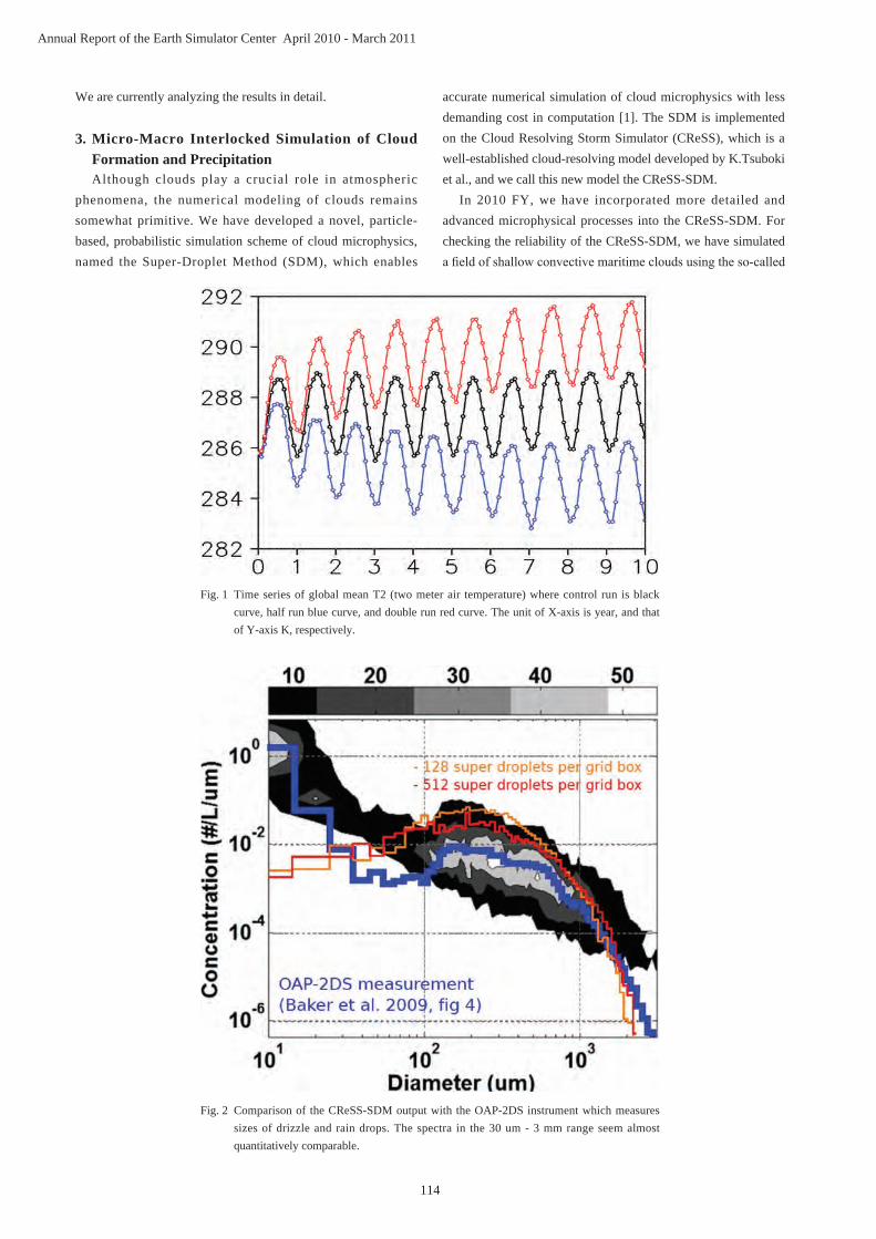
114


We are currently analyzing the results in detail.

3. Micro-Macro Interlocked Simulation of Cloud Formation and PrecipitationAlthough clouds play a crucial role in atmospheric

phenomena, the numerical modeling of clouds remains somewhat primitive. We have developed a novel, particle-based, probabilistic simulation scheme of cloud microphysics, named the Super-Droplet Method (SDM), which enables

accurate numerical simulation of cloud microphysics with less demanding cost in computation [1]. The SDM is implemented on the Cloud Resolving Storm Simulator (CReSS), which is a well-established cloud-resolving model developed by K.Tsuboki et al., and we call this new model the CReSS-SDM.

In 2010 FY, we have incorporated more detailed and advanced microphysical processes into the CReSS-SDM. For checking the reliability of the CReSS-SDM, we have simulated a field of shallow convective maritime clouds using the so-called

Fig. 2 Comparison of the CReSS-SDM output with the OAP-2DS instrument which measures sizes of drizzle and rain drops. The spectra in the 30 um - 3 mm range seem almost quantitatively comparable.

Fig. 1 Time series of global mean T2 (two meter air temperature) where control run is black curve, half run blue curve, and double run red curve. The unit of X-axis is year, and that of Y-axis K, respectively.

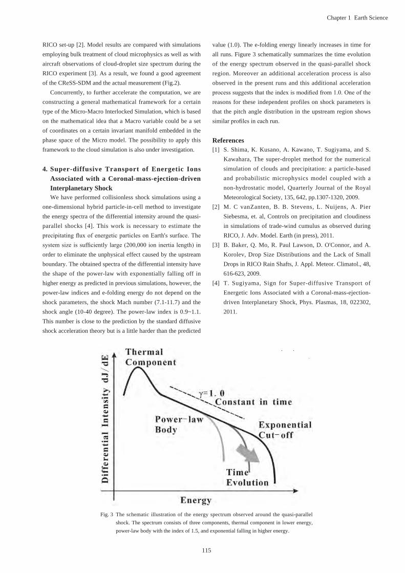
115


RICO set-up [2]. Model results are compared with simulations employing bulk treatment of cloud microphysics as well as with aircraft observations of cloud-droplet size spectrum during the RICO experiment [3]. As a result, we found a good agreement of the CReSS-SDM and the actual measurement (Fig.2).

Concurrently, to further accelerate the computation, we are constructing a general mathematical framework for a certain type of the Micro-Macro Interlocked Simulation, which is based on the mathematical idea that a Macro variable could be a set of coordinates on a certain invariant manifold embedded in the phase space of the Micro model. The possibility to apply this framework to the cloud simulation is also under investigation.

4. Super-diffusive Transport of Energetic Ions Associated with a Coronal-mass-ejection-driven Interplanetary ShockWe have performed collisionless shock simulations using a

one-dimensional hybrid particle-in-cell method to investigate the energy spectra of the differential intensity around the quasi-parallel shocks [4]. This work is necessary to estimate the precipitating flux of energetic particles on Earth's surface. The system size is sufficiently large (200,000 ion inertia length) in order to eliminate the unphysical effect caused by the upstream boundary. The obtained spectra of the differential intensity have the shape of the power-law with exponentially falling off in higher energy as predicted in previous simulations, however, the power-law indices and e-folding energy do not depend on the shock parameters, the shock Mach number (7.1-11.7) and the shock angle (10-40 degree). The power-law index is 0.9~1.1. This number is close to the prediction by the standard diffusive shock acceleration theory but is a little harder than the predicted

value (1.0). The e-folding energy linearly increases in time for all runs. Figure 3 schematically summarizes the time evolution of the energy spectrum observed in the quasi-parallel shock region. Moreover an additional acceleration process is also observed in the present runs and this additional acceleration process suggests that the index is modified from 1.0. One of the reasons for these independent profiles on shock parameters is that the pitch angle distribution in the upstream region shows similar profiles in each run.

References[1] S. Shima, K. Kusano, A. Kawano, T. Sugiyama, and S.

Kawahara, The super-droplet method for the numerical simulation of clouds and precipitation: a particle-based and probabilistic microphysics model coupled with a non-hydrostatic model, Quarterly Journal of the Royal Meteorological Society, 135, 642, pp.1307-1320, 2009.

[2] M. C vanZanten, B. B. Stevens, L. Nuijens, A. Pier Siebesma, et. al, Controls on precipitation and cloudiness in simulations of trade-wind cumulus as observed during RICO, J. Adv. Model. Earth (in press), 2011.

[3] B. Baker, Q. Mo, R. Paul Lawson, D. O'Connor, and A. Korolev, Drop Size Distributions and the Lack of Small Drops in RICO Rain Shafts, J. Appl. Meteor. Climatol., 48, 616-623, 2009.

[4] T. Sugiyama, Sign for Super-diffusive Transport of Energetic Ions Associated with a Coronal-mass-ejection-driven Interplanetary Shock, Phys. Plasmas, 18, 022302, 2011.

Fig. 3 The schematic illustration of the energy spectrum observed around the quasi-parallel shock. The spectrum consists of three components, thermal component in lower energy, power-law body with the index of 1.5, and exponential falling in higher energy.

116


宇宙・地球表層・地球内部の相関モデリング


草野　完也　　海洋研究開発機構　地球内部ダイナミクス領域

著者草野　完也 *1，大淵　　済 *2，島　伸一郎 *1，杉山　　徹 *1，力石　裕介 *3



*3 東京工業大学　大学院理工学研究科

地球環境システムは内部（地殻、マントル、コア）、表層（大気海洋）および外部（宇宙）が互いに影響を及ぼしながら変動進化する相関システムである。本プロジェクトは地球環境の大規模変動と宇宙及び地球内部ダイナミクスの関係を探るために、先進的な相関モデルを開発する目的で 2009年度より開始された。本プロジェクトでは、特に宇宙線と雲の関係に注目しその物理的関係を定量的に解明するため、ミクロスケールからマクロスケールに至る様々な物理過程を可能な限り第 1原理に基づいてモデル化すると共に、それらのモデルを総合した包括的な宇宙地球システムモデルを構築することを目指している。2010年度は、エアロゾルの核形成に関する分子シミュレーション、超水滴法を利用した積雲成長シミュレーション、プラズマ中の高エネルギー粒子加速過程のシミュレーションについてそれぞれ発展させた、さらに、大気海洋結合全球循環モデルを用いて銀河宇宙線の影響によって生成されると考えられている雲凝結核の変化による気候変動に関するシミュレーション研究を新たに開始した。

キーワード : 宇宙天気 , 宇宙気候 , マルチスケール , マルチフィジックス , プラズマ , 雲 , オーロラ , 核形成 , エアロゾル , 粒子加速 , 地球シミュレータ

Chapter 2

Epoch-Making Simulation

119


1. OverviewConstruction of a software infrastructure for highly parallel

computing environments requires precisely prediction of future hardware technologies, and design of scalable and portable software for these technologies.

The Scalable Software Infrastructure for Scientific Computing (SSI). Project was initiated in November 2002, as a national project in Japan, for the purpose of constructing a scalable software infrastructure [1], [2], [3]. Based on the policies, we have used various types of parallel computers, and carefully designed our libraries on them, to maintain portability and usability. The architectures included shared-memory parallel computers, distributed-memory parallel computers, and vector supercomputers. Since 2006, the SSI project has been selected for a joint research with the Earth Simulator Center to port our libraries on massively parallel vector computing environments. Since 2003, we have signed a contract with the IBM Watson Research Center on the joint study of library implementation on massively parallel environments with tens of thousands of processors. The results of the SSI project will be evaluated on larger computers in the near future.

In the SSI project, we have studied object-oriented implementation of libraries, autotuning mechanisms, and languages for the implemented libraries. The results were applied to a modular iterative solver library Lis and a fast Fourier transform library FFTSS. The libraries were written in C and equipped with Fortran interfaces. We have also developed a simple interface for library collections SILC, with an extension to scripting language.

2. Lis: a Library of Iterative Solvers for Linear Sytems In the fields such as fluid dynamics and structural analysis,

we must solve large-scale systems of linear equations with sparse matrices to compute high resolution numerical solutions of partial differential equations. We have developed Lis, a library of iterative solvers and preconditioners with various sparse matrix storage formats. Supported solvers, preconditioners, and matrix storage formats are listed in Table. 1-4. We present an example of the program using Lis in Fig. 1.

There are a variety of portable software packages that are applicable to the iterative solver of sparse linear systems. SPARSKIT is a toolkit for sparse matrix computations written in Fortran. PETSc is a C library for the numerical solution of partial differential equations and related problems, which is to be used in application programs written in C, C++, and Fortran. PETSc includes parallel implementations of iterative solvers and preconditioners based on MPI. Aztec is another library of parallel iterative solvers and preconditioners written in C. The library is fully parallelized using MPI. From the viewpoint of functionality, our library and all three of the libraries mentioned above support different sets of matrix storage formats, iterative solvers, and preconditioners. In addition, our library is parallelized using OpenMP with the first-touch policy and takes the multicore architecture into consideration. Many feedbacks from the users have been applied to Lis, and Lis has been tested on various platforms from small personal computers with Linux, Macintosh, and Windows operating systems to massively parallel computers, such as NEC SX, IBM Blue Gene, and Cray XT series. Major tested platforms and target options are listed in Table. 5-6. The code of Lis has attained the vectorization

Development of General Purpose Numerical Software Infrastructure for Large Scale Scientific Computing


Akira Nishida Research Institute for Information Technology, Kyushu University

Author

Akira Nishida Research Institute for Information Technology, Kyushu University

The Scalable Software Infrastructure Project was initiated as a national project in Japan for the purpose of constructing a scalable parallel software infrastructure for scientific computing. The project covered three areas: iterative solvers for linear systems, fast integral transforms, and their portable implementation.

Modular programming was adopted to enable users to write their codes by combining elementary mathematical operations. Implemented algorithms were selected from the viewpoint of scalability on massively parallel computing environments. Since the first release in September 2005, the codes have been used by thousands of research projects around the world.

Keywords: high performance computing, parallel algorithms, modular programming

120


Table 1 Solvers for linear equations.

1.0.x

CG

Added in 1.1.x

CRBiCG BiCR CGS CRS BiCGSTAB BiCRSTAB BiCGSTAB(l) GPBiCR GPBiCG BiCRSafe Orthomin(m) FGMRES(m)GMRES(m) IDR(s) TFQMR MINRESJacobiGauss-SeidelSOR

Table 2 Solvers for eigenproblems.

Added in 1.2.0

Power IterationInverse IterationApproximate Inverse IterationConjugate GradientLanczos IterationSubspace IterationConjugate Residual

Table 3 Preconditioners.

1.0.x

Jacobi

Added in 1.1.0

Crout ILUILU(k) ILUTSSOR Additive SchwarzHybrid User defined preconditionerI+SSA-AMGSAINV

Table 4 Matrix storage formats.

Point

Compressed Row StorageCompressed Column StorageModified Compressed Sparse RowDiagonalEllpack-Itpack generalized diagonalJagged Diagonal StorageDenseCoordinate

BlockBlock Sparse RowBlock Sparse ColumnVariable Block Row

121


Table 5 Major tested platforms.

C compilers OSIntel C/C++ Compiler 7.0, 8.0, 9.1, 10.1, 11.1, Intel C++ Composer XE

Linux Windows

IBM XL C/C++ V7.0, 9.0 AIX Linux

Sun WorkShop 6, Sun ONE Studio 7, Sun Studio 11, 12 Solaris

PGI C++ 6.0, 7.1, 10.5 Linux

gcc 3.3, 4.3Linux Mac OS X Windows

Microsoft Visual C++ 2008, 2010 WindowsFortran compilers (optional) OS

Intel Fortran Compiler 8.1, 9.1, 10.1, 11.1, Intel Fortran Composer XE

Linux Windows

IBM XL Fortran V9.1, 11.1 AIX Linux

Sun WorkShop 6, Sun ONE Studio 7, Sun Studio 11, 12 Solaris

PGI Fortran 6.0, 7.1, 10.5 Linuxg77 3.3 gfortran 4.3, 4.4 g95 0.91

Linux Mac OS X Windows

Table 6 Major target options.

<target> Configure scriptscray_xt3 ./configure CC=cc FC=ftn CFLAGS="-O3 -B -fastsse -tp k8-64"

FCFLAGS="-O3 -fastsse -tp k8-64 -Mpreprocess" FCLDFLAGS="-Mnomain"ac_cv_sizeof_void_p=8 cross_compiling=yes --enable-mpiax_f77_mangling="lower case, no underscore, extra underscore"

fujitsu_pq ./configure CC=fcc FC=frt ac_cv_sizeof_void_p=8CFLAGS="-O3 -Kfast,ocl,preex" FFLAGS="-O3 -Kfast,ocl,preex -Cpp"FCFLAGS="-O3 -Kfast,ocl,preex -Cpp -Am"ax_f77_mangling="lower case, underscore, no extra underscore"

hitachi ./configure CC=cc FC=f90 FCLDFLAGS="-lf90s" ac_cv_sizeof_void_p=8CFLAGS="-Os -noparallel" FCFLAGS="-Oss -noparallel"ax_f77_mangling="lower case, underscore, no extra underscore"

ibm_bgl ./configure CC=blrts_xlc FC=blrts_xlf90CFLAGS="-O3 -qarch=440d -qtune=440 -qstrict-I/bgl/BlueLight/ppcfloor/bglsys/include"FFFLAGS="-O3 -qarch=440d -qtune=440 -qsuffix=cpp=F -qfixed=72 -w-I/bgl/BlueLight/ppcfloor/bglsys/include"FCFLAGS="-O3 -qarch=440d -qtune=440 -qsuffix=cpp=F90 -w-I/bgl/BlueLight/ppcfloor/bglsys/include"ac_cv_sizeof_void_p=4 cross_compiling=yes --enable-mpiax_f77_mangling="lower case, no underscore, no extra underscore"

nec_es ./configure CC=esmpic++ FC=esmpif90 AR=esar RANLIB=trueac_cv_sizeof_void_p=8 ax_vector_machine=yes cross_compiling=yes--enable-mpi --enable-ompax_f77_mangling="lower case, no underscore, extra underscore"

nec_sx9_cross ./configure CC=sxmpic++ FC=sxmpif90 AR=sxar RANLIB=trueac_cv_sizeof_void_p=8 ax_vector_machine=yes cross_compiling=yesax_f77_mangling="lower case, no underscore, extra underscore"5

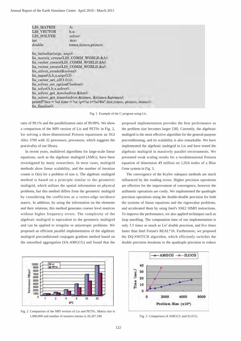
122


ratio of 99.1% and the parallelization ratio of 99.99%. We show a comparison of the MPI version of Lis and PETSc in Fig. 2, for solving a three-dimensional Poisson equationon an SGI Altix 3700 with 32 processors, processors, which suggests the practicality of our library.

In recent years, multilevel algorithms for large-scale linear equations, such as the algebraic multigrid (AMG), have been investigated by many researchers. In most cases, multigrid methods show linear scalability, and the number of iteration counts is O(n) for a problem of size n. The algebraic multigrid method is based on a principle similar to the geometric multigrid, which utilizes the spatial information on physical problems, but this method differs from the geometric multigrid by considering the coefficient as a vertex-edge incidence matrix. In addition, by using the information on the elements and their relations, this method generates coarser level matrices without higher frequency errors. The complexity of the algebraic multigrid is equivalent to the geometric multigrid and can be applied to irregular or anisotropic problems. We proposed an efficient parallel implementation of the algebraic multigrid preconditioned conjugate gradient method based on the smoothed aggregation (SA-AMGCG) and found that the

proposed implementation provides the best performance as the problem size becomes larger [38]. Currently, the algebraic multigrid is the most effective algorithm for the general-purpose preconditioning, and its scalability is also remarkable. We have implemented the algebraic multigrid in Lis and have tested the algebraic multigrid in massively parallel environments. We presented weak scaling results for a twodimensional Poisson equation of dimension 49 million on 1,024 nodes of a Blue Gene system in Fig. 3.

The convergence of the Krylov subspace methods are much influenced by the rouding errors. Higher precision operations are effective for the improvement of convergence, however the arithmetic operations are costly. We implemented the quadruple precision operations using the double-double precision for both the systems of linear equations and the eigenvalue problems, and accelerated them by using Intel's SSE2 SIMD instructions. To improve the performance, we also applied techniques such as loop unrolling. The computation time of our implementation is only 3.5 times as much as Lis' double precision, and five times faster than Intel Fortan's REAL*16. Furthermore, we proposed the DQ-SWITCH algorithm, which efficiently switches the double precision iterations to the quadruple precision to reduce

Fig. 2 Comparison of the MPI version of Lis and PETSc. Matrix size is 1,000,000 and number of nonzero entries is 26,207,180. Fig. 3 Comparison of AMGCG and ILUCG.

Fig. 1 Example of the C program using Lis.

123


the computation time. The idea of the SIMD accelerated double-double precision operations was incorporated into Japan's next generation 10 petaflops supercomputer project by RIKEN.

In structural analysis and materials science such as solid-state physics and quantum chemistry, efficient algorithms for large-scale eigenproblems for large-scale simulations are indispensable. There are several methods to compute eigenvalues of large-scale sparse matrices. We implemented major algorithms based on the Krylov subspace, from the viewpoint of scalability in parallel environments. The eigenproblems can be solved combined with appropriate preconditioners, including the algebraic multigrid.

The performance of iterative solvers is affected by the data structure of given matrices, the methodology of their parallelization, and the hierarchy of computer architectures. We have studied the validity of the performance optimization of iterative solvers by benchmarking the MFLOPS performance of matrix vector product kernels on the given computing environment. Figure 4 shows the performance of a kernel spmvtest1, derived from a discretized 1-dimensional Poisson equation, for size from up to 1,280,000 on a single node of SX-9 at JAMSTEC, and Fig. 5-7 show the performance for size up to 40,960,000 on three scalar clusters with DDR Infiniband interconnect at Kyushu University. While the scalar architecture based machines show performance degradation after they reach their peak performance with the data size of 500kB to 2MB per

core, vector architecture shows gradual performance increase until it reaches about 8-9GFLOPS per core (with the diagonal (DIA) format in this case), and keep it as the data size grows. It suggests that we should use as many cores with large caches as possible when using a scalar architecture for such problems.

To date, we have counted more than three thousand projects around the world. It is just the first step for us to achieve more flexibility in scalable scientific computing, but we hope our efforts reduce some barriers towards upcoming exascale scientific computing environments in the near future.

References[1] A. Nishida, "SSI: Overview of simulation software

infrastructure for large scale scientific applications (in Japanese)", IPSJ, Tech. Rep. 2004-HPC-098, 2004.

[2] A. Nishida, "Experience in Developing an Open Source Scalable Software Infrastructure in Japan", Lecture Notes in Computer Science, vol. 6017, pp. 87-98, 2010.

[3] A. Nishida, R. Suda, H. Hasegawa, K. Nakajima, D. Takahashi, H. Kotakemori, T. Kajiyama, A. Nukada, A. Fujii, Y. Hourai, S. L. Zhang, K. Abe, S. Itoh, and T. Sogabe, The Scalable Software Infrastructure for Scientific Computing Project, Kyushu University, 2009, http://www.ssisc.org/.

Fig. 4 Performance of spmvtest1 for size from 40,000 to 1,280,000 on a single node of the Earth Simulator 2.

010,00020,00030,00040,00050,00060,00070,000

MFL

OP

S

1 2 4 8 CRSBSR

#cores

CRS

CCS

MSR

DIA

ELL

JDS

BSR

BSC

COO

Fig. 5 Performance of spmvtest1 for size from 320,000 to 40,960,000 on the Fujitsu PRIMEGY RX200S3 Cluster at Kyushu University.

0100,000200,000300,000400,000500,000600,000

MFL

OP

S

256 1024 CRS#cores

CRS

CCS

MSR

DIA

ELL

JDS

BSR

BSC

COO

Fig. 6 Performance of spmvtest1 for size from 160,000 to 40,960,000 on the Fujitsu PRIMEQUEST Cluster at Kyushu University.

0

100,000

200,000

300,000

400,000

MFL

OP

S

128 CRS#cores

CRS

CCS

MSR

DIA

ELL

JDS

BSR

BSC

COO

Fig. 7 Performance of spmvtest1 for size from 1,280,000 to 40,960,000 on the Hitachi SR16000 Cluster at Kyushu University.

0200000400000600000800000

10000001200000

MFL

OP

S

512 CRSBSC

#cores

CRS

CCS

MSR

DIA

ELL

JDS

BSR

BSC

COO

124


大規模科学計算向け汎用数値ソフトウェア基盤の開発


西田　　晃　　九州大学　情報基盤研究開発センター

著者西田　　晃　　九州大学　情報基盤研究開発センター

本プロジェクトでは、従来それぞれの分野において別個に進められてきた並列アルゴリズムや実装に関する知見をもとに、大規模化が予想される今後の計算環境に対応したスケーラブルなソフトウェア基盤を整備することを目的として、反復解法、高速関数変換、及びその効果的な計算機上への実装手法を中心に、平成 14年度より科学技術振興機構戦略的創造研究推進事業の一環として、多様な計算機環境を想定した開発を行っている。モジュール化されたインタフェースを採用し、複雑な機能を持つライブラリを容易に構築できるようにするとともに、スケーラビリティの観点から並列化に適したアルゴリズムを開発、実装し、高並列な環境での使用に耐えるライブラリを実現している。本研究の成果はネットワークを通じて広く一般に配布し、フィードバックをもとにより汎用性の高いソフトウェアとしていく方針を採っており、平成 17年 9月よりソースコードを無償公開するとともに、ユーザの要望を反映した更新を適宜行なっている。平成 18年度からは、地球シミュレータセンター共同プロジェクトの一環として、高並列なベクトル計算機環境への最適化を実施し、その成果をライブラリとして公開し、多くのユーザに利用されている。本年度は小規模利用環境への移植を中心に行うとともに、4倍精度演算を用いた固有値解法ライブラリを実装し、その有効性を実証した。

キーワード : ハイパフォーマンスコンピューティング , 並列アルゴリズム , モジュラープログラミング

125


1. INTRODUCTIONNano-carbon materials have been expected to bring

breakthrough to material science and nanotechnology. A lot of potential applications of nanotube and fullerene to electronic devices have been attracted to scientists and engineers.

In the present days, large-scale numerical simulation by using supercomputer's computational performance has turned to be a very efficient tool and leverage for investigating their novel material properties. It now allows us to simulate complex nano-structures with more than ten thousand atom of carbon

Aiming at using large-scale simulations on the Earth Simulator, we have developed an application package of ab initio DFT theory and parameterized tight-binding (TB) models. Especially, the TB model shows that it is very suitable for the very large systems even if it has a lack of symmetrical arrangement.

In this term, we have carried out simulation studies, in

which there are three primary objectives as (1) design of innovative nonmaterial with the required properties; (2) obtain fundamental properties in nano-scale matter, and (3) develop new applications.

2. Physical studies on nano materials2.1 Application of Novel Functions of Mackay Crystal to

Solar Cell [1]

We have carried out the extensive simulation on the Mackay crystals using GSW method to find synthesis process and DFT approximation to obtain mechanical and electrical properties. In 2009, from the investigation on electronic properties of Mackay crystals, it was indicated that the band gap of Mackay crystals of P48, P144 and P192 are ranged from 0.05eV to 0.94 eV. On the basis of this prediction, we proposed that a tandem-type solar cell could be conceptually designed by stacking Mackey crystal films with the different size. This solar cell would be able to

Large Scale Simulations for Carbon Nanotubes


Syogo Tejima Research Organization for Information Science & Technology

Authors

Syogo Tejima*1, Satoshi Nakamura*1, Yoshiyuki Miyamoto*2, Yoshikazu Fujisawa*3 and Hisashi Nakamura*1

*1 Research Organization for Information Science & Technology (RIST)

*2 R&D Unit Central Res. Labs. Green Innovation Research Laboratories, NEC Corporation

*3 Honda R&D Co., Ltd.

CARBON NANOTUBE RESEARCH GROUP

Morinobu Endo, Eiji Osawa, Atushi Oshiyama, Yasumasa Kanada, Susumu Saito, Riichiro Saito, Hisanori Shinohara, David Tomanek, Tsuneo Hirano, Shigeo Maruyama, Kazuyuki Watanabe, Takahisa Ohno, Yutaka Maniwa, Yoshikazu Fujisawa, Yoshiyuki Miyamoto, Hisashi Nakamura

Nano carbon materials as nanotube, fullerene and graphen have a potential for applications to the advanced industries. For nano carbon materials, it has been recognized as large-scale simulation is a powerful and efficient tool to find and create new functional nano carbon materials.

Aiming at conducting the productive simulation for nano-materials, we have developed the large-scale simulation models such as tight-binding molecular dynamic model, ab-initio density functional theory (DFT), and time-dependent DFT model.

In this term, by utilizing these models effectively, we have studied various physical properties of nano-carbon and applications such as (1) application of novel functions of Mackay Crystal to solar cell, (2) Large-scale Simulation on Electron Conduction in Carbon Nanotubes at Finite Temperature, (3) applications of time-dependent density functional theory for photo-chemical reaction of molecules inside CNTs. Along these works, we have realized as the Earth Simulator is a very powerful tool for large-scale nano-material simulations.

Keywords: Large scale simulation, TB theory, ab initio theory, Time-dependent DFT, Carbon Nanotube, Fullerenes, Graphene, Mackay crystal, solar cell, Green energy, quantum electronic transport, photoelectric material

126


absorb the sun light with near infrared light.The electrical energy is converted from photon energy of

solar cell. In order to derive electrical energy from the Mackay crystal, we have to set p-n semi-conductance junction. In this year, we have simulated the electronic structure of Mackay crystals with Nitrogen and Boron as the doping material for producing p-n Mackay junction. Nitrogen and Boron inject electrons and holes into the crystal as the carrier mobility, respectively, into the crystal. Figures 1 and 2 show the energy-dependence of doping materials inserted to different atomic sites. From these figures, it is clear that the doped atomic site is surrounded by only hexagons and by two hexagon and octagon in fig. 3, respectively. The replaced energy measured from pure crystal is also exhibited at the right side in Figs. 1 and 2. The simulation has revealed the doping of Nitrogen and Boron are more stable at octagonal than hexagonal one.

Figures 3 and 4 show the electrical density of state for Nitrogen and Boron doping to the octagonal site. The N-doping (B-doping) leads to the injection of holes (electrons) as shown in Fig. 3 (Fig. 5). Such as band structure indicates N- and B-doping to Mackay crystal can lead to a carrier of hole and electrons in the crystal.

As the next step, from valence-conduction band transition probability, we plan to simulate the photon energy absorption

efficiency. Mackay crystals are expected to be a highly efficient photoelectric material for solar cell.

2.2 Large-scale simulation on electron conduction of car-bon-nanotubes in finite-temperature environments [2]

The rapid development of integrated circuit technology is primarily achieved due to the sustained downscaling in the metal-oxide-semiconductor field effect transistor (MOSFET). Moore's law is a phenomenological observation that the number of transistors on integrated circuits doubles every two years. Silicon-based MOS technology, however, is considered to face technical and economical limits as soon as at the end of this decade. Therefore, new types of nanoscale devices are being investigated aggressively. In this context, a lot of attention is paid to integrated circuits made of carbon-nanotubes (CNTs). In nano-scale systems, the macroscopic Ohm's law breaks down due to the various effects caused by finite size effects. Here one needs to study the transport behavior of CNTs using a quantum mechanical description.

Our group has been developing an order-N code for simulating electron conduction. Our approach is based on the non-equilibrium Green's function (NEGF) formalism which is the method of choice to evaluate electron conductance in nanostructure.

Fig. 1 A carbon surrounded only hexagon is replaced by Boron and Nitrogen atom. Replaced energy is described at the right side.

Fig. 2 A carbon surrounded two hexagons and a octagon are replaced by Boron and Nitrogen atoms. Replaced energy is described at the right side.

Fig. 3 The N-doping leads to injection of electron in the energy band.

Fig. 4 The B-doping leads to injection of hole in the energy band.

127


Jj1 → j2

= 2e∑ t j2ξ2 j1ξ1({R})∫{ f (ɛ–μR) – f (ɛ–μL)}hξ1ξ2

× ∑Re[Ĝ σ

rCC

aCC (ɛ)](ɛ){–iГLL(ɛ)}G dɛ( j1,ξ1,σ ) ( j2,ξ2,σ )

,

where the retarded and advanced NEGFs are defined as follow:

Ĝ r (ɛ) = =CC

ÎCC (ɛ+iγ) ICC – HCC –Σr (ɛ) – Σr (ɛ)

LL

RR ,

Ĝ a (ɛ) = =CC

ÎCC (ɛ+iγ) ICC – HCC –Σa (ɛ) – Σa (ɛ)

LL

RR .

The true electron conduction is obtained by taking the limit as g tends to positive zero. In order to calculate the NEGFs in the above equations, we have adopted the embedding potential method which works well on treating quasi-one-dimensional systems such as carbon-nanotubes. This method provides an algorithm of the order-N, indicating the possibility of performing high-performance computation in large-scale models. The NEGF formalism can also be applied to CNTs of arbitrary chirality or CNTs with defects.

Moreover, by solving self-consistently the coupled NEGF and three-dimensional Poisson equations, we can obtain the electrostatic potential distribution in carbon-nanotubes. In this case, we need to solve the Poisson equation as fast as possible. A promising method for this is to use the substitute charge method. However, since the conventional substitute charge method determines the values of the charges on the basis of empirically-predicted charge distribution, this method has the problem that its calculation accuracy depends on how to select the substitute charge distribution. Therefore, we have developed a new method by changing not only the values of the charges but also their positions. Our method allows us to impose the Dirichlet boundary conditions on three-dimensional surfaces with arbitrary shape and to treat even problems with incomplete boundary conditions. In addition, once the substitute charge distribution is determined, there is no need to repeat this procedure any more. This makes efficient and stable calculation

possible. As an application of our substitute charge method, we consider the system consisting of one gate and two electrodes as shown in Fig.5 (a), where the gate voltage is 2.0 eV and the bias applied between two electrodes is 1.0 eV. Then, the effect of the gate and electrodes is represented by the substitute charges as shown in Fig. 5 (b).

Now, in order to simulate microscopic electron conduction at atomic scale using our method, we need to calculate NEGFs of which number is equal to the number of mesh points used in numerical integration with respect to energy. On the one hand, the accuracy of calculation increases with the increase of the number of mesh points; on the other hand, the number of mesh points needed to obtain reliable estimates of the electron conduction increases inversely proportionally with the strength of nanotube-electrode junction. As a result, when the strength of the junction is comparatively small, it takes enormous computing time to simulate the electron conduction. To overcome this difficulty, we have developed a method for computing the NEGFs with high accuracy and high speed by applying analytic continuation via the Pade approximants. An example of our method is shown in Fig. 6. We first have simulated NEGFs at g = 0.00094278 eV through the embedding potential method and computed the electron current indicated by the green circle. Using these NEGFs as input data of the Pade approximants, we obtained the electron currents represented by the blue triangles. Finally, applying the Pade approximants again to the values of the electron current corresponding to different values of g, we obtained the ideal results which are obtained in the limit as g tends to positive zero (the red lozenge in Fig. 6).

According to the simulation results using 80 nodes (640 processors) on the Earth Simulator, it took about 1,800 sec to compute all the NEGFs with out method. On the other hand, when all the NEGF is computed directly without the Pade approximants, it took about 5,100 sec to perform the same simulations. Hence, our method is about 2.8 more effective than that without the Pade approximants.

Fig. 5 (a) Schematic view of the system consisting one gate and two electrodes; (b) the different color dots represent different values of the substitute charge.

(a) (b)

128


2.3 Application of time-dependent density functional theory for photo-chemical reaction of molecules inside CNTs [3]

Following 2009, application of femto-second laser was investigated for photo-chemical reaction of molecules inside CNTs. Since molecules in gas phase are dilute and thus has low cross-section of photo-irradiation, confining molecules into nano-space was expected effective to increase the cross-section. A question here is whether there is proper material which can confine molecules in narrow space and can penetrate optical field. We tested semiconducting (8,0) CNT, and discovered this CNT works as nano-test-tube. We performed electron-ion dynamics under present of pulse laser with alternating electric field mimicking the laser pulse by solving time-dependent Kohn-Sham equation

iħ dΨn (r, t) = {HKS (r, t) + Vext (r, t)}Ψn (r, t) ,dt

which includes scalar potential mimicking optical field.An HCl molecule was chosen as our case study, which is

historically studied as a subject of photo-induced disintegration. When this is encapsulated inside (8,0) nanotube exothermically,

this molecule can be disintegrated as following figure with ultra-short femto-second laser pulse with corresponding power is 1.91x1015W/cm2.

This result will stimulate experimental work in nanotube community and been published in Physical Review Letters in 2010, as well as the last year's product (laser-induced graphene exfoliation). Because of the mass difference, only H atom obtained high kinetic energy which is enough to move outside from the open-end of the CNT into the vacuum. We expect that pulse laser can extract from any molecule that contains H atom being encapsulated by CNT.

This year, we are exploring more complex situation, i.e., a molecular dimer of acetylene which never exists in natural gas phase but can exist in CNT. Pulse-induced synchronized motion of two molecules inside CNT is monitored by the simulation. We expect that further time-simulation will reveal a new path of chemical reaction of these molecules.

3. SUMMARYLarge-scale simulat ions have been carried out on

nonmaterial by using ab initio density functional theory and the parameterized tight-binding models. These optimized models allowed us to simulate the nano maretial properties with excellent performance on the Earth Simulator. It enables us to come across discoveries of novel phenomena in nano scale and to find out some useful materials for clean energies and nano device.

References [1] S. Tejima, Nikkei newspaper, Sep 30 (2010).[2] S. Nakamura,et al . , NT10 Eleventh International

Conference on the Science and Application of Nanotubes, Montreal, June 26 (2010).

[3] S. Miyamoto, et al., Phys Rev lett Vol.105 pp248301-1-248301(2010).

Fig. 6 The green circle was calculated via the embedding potential method. The blue triangles were evaluated from the Pade approximants of which input data are the NEGFs at g = 0.00094278 eV. The red lozenge is estimated using the value of the blue triangles as input data of the Pade approximants.

Fig. 7 Dynamics of an HCl inside (8,0) CNT.

129


カーボンナノチューブの特性に関する大規模シミュレーション


手島　正吾　　高度情報科学技術研究機構

著者手島　正吾 *1，中村　　賢 *1，宮本　良之 *2，藤沢　義和 *3，中村　　壽 *1

*1 高度情報科学技術研究機構

*2 NEC R&D ユニット　中央研究所　グリーンイノベーション研究所

*3 本田技術研究所

1. 研究目的優れた物性が予想されナノテクの基本材であるナノ炭素類（カーボンナノチューブ（CNT）、フラーレン、グラフェン）

の電子・機械特性を従来不可能だった大規模シミュレーションにより推定し、科学技術及び産業界に提供すると共に、応用として特性の優れた新構造を発見し、基本材の拡充に寄与する目的で実施された。

2. 成果これまで、我が国のナノチューブ研究で当面する課題解決に向けた応用シミュレーションを実施した。本年度さらに、

グリーンエネルギーに関するシミュレーションを推進した。得られた結果を以下に示す。（1）これまでマッカイ結晶の包括的な特性把握のために、合成法、機械特性などのシミュレーションを実施してきた。

昨年度は、電子構造特性のシミュレーションにより、マッカイ結晶が太陽電池材料としての可能性があることが示せた。本年度は、光電変換で生じた電気エネルギーを外部に取り出す為に、キャリアを持つを p-n半導体を作りその特性を調べた。ホールと電子のキャリアを挿入するためのドーピング元素としてホウ素と窒素を選んだ。全エネルギー計算の結果、ドーピング元素がマッカイ結晶の８員環の原子の一部を置換し易いことが明らかになった。また、置換された結晶の電子状態密度から、ホウ素置換では価電子帯にホールが、窒素置換では伝導体に電子がそれぞれ出現することが明らかになった。キャリアが導入されことにより、太陽電池として n-p型半導体ジャンクションを利用して電流を外部に導く機能を得る事ができた。積層半導体マッカイ結晶は、応用として、広範囲の波長の光吸収を可能とする、高効率太陽が期待される。

（2）本研究では、非平衡グリーン関数（NEGF）法を用いた伝導特性計算において、CNTのような擬 1次元系で威力を発揮する埋め込みポテンシャル法を用いたアルゴリズムを採用し、オーダー N 法の量子伝導シミュレーションコードを開発している。NEGF法では、ポテンシャル分布を求める際にポアソン方程式を高速に解く必要がある。そこで、電荷の値だけでなく電荷の位置も変化させることができる新たな電荷代用法を開発し、これにより高速で安定した計算を可能にした。これらの手法を用いて原子スケールでの微視的な電流をシミュレーションするには、エネルギーに関する数値積分での分点の数だけ NEGFを計算する必要がある。高速化を目的に、パデ近似による解析接続を用いて NEGFを高い精度で高速に求める計算手法を開発し、計算時間を 3分の 1程度に減らすことに成功した。

（3）ナノチューブ内分子分解反応の第一原理時間発展計算によるシミュレーション実施した。フェムト秒レーザショットの強さを制御するとナノチューブ内部で HCl分子は自然に分解する現象が生じた。この結果は、カーボンナノチューブを使って分子の光化学反応の過程が進行する事を示している。

キーワード : 大規模シミュレーション , タイトバインディング理論 , 時間依存密度汎関数法 , カーボンナノチューブ , グラフェン , マッカイ結晶 , 太陽電池 , グリーンエネルギー , 量子伝導 , 光電材料 , 光化学反応

131


1. IntroductionFor the realization of sustainable society in the 21 century,

assessment of gradually aging social infrastructure is becoming important. Fracture analysis has been one of the key numerical simulation for such problems. However, a three dimensional crack analysis of a real world, highly complicated structure has not been widely used yet, because of many obstacles including the lack of computational power.

The authors have been developing an open-source CAE system, ADVENTURE [1]. It is based on the hierarchical domain decomposition method (HDDM) with the balancing domain decomposition (BDD) pre-conditioner [2,3]. A general-purpose structural analysis solver, ADVENTURE Solid is one of the solver modules of the ADVENTURE system. On the other hand, we have also been developing a system to support a three dimensional fracture analysis[4], especially a fatigue or SCC propagation analysis with many cracks of arbitrary complicated shape and orientation. To integrate the large scale structural analysis code with this fully automatic fracture analysis capability, a direct fracture simulation of a highly complicated realistic aging structure with explicit modeling of cracks.

In this year, we conducted mainly two tasks, performance tuning of ADVENTURE Solid for ES2 and developing mesh refinement function for ADVENTURE Metis to generate large model of over tens-of-billions DOFs.

2. Performance Optimization of ADVENTURE SolidAs a continued effort to optimize our structural analysis

code, ADVENTURE Solid, on The Earth Simulator 2, we have chosen two approaches. One is to optimize the ADVENTURE Solid code within the range of the existing design, by varying a few selected performance-sensitive parameters. The other is to apply more drastic design changes, such as the local Schur complement approach, already described briefly in the last year's ES report.

Here, the performance design issues of ADVENTURE Solid are briefly explained. ADVENTURE Solid is based on the hierarchical domain decomposition method (HDDM). In HDDM, a whole analysis domain is subdivided into many small subdomains. The parallelization of ADVENTURE Solid code is primarily based on subdomain-wise FEM calculation. On the FE analysis of each subdomain, a linear system of the subdomain stiffness matrix is solved. A skyline solver is employed for the solution of the relatively small system. In the current version of ADVENTURE Solid, this subdomain-wise skyline solver is identified as a hot spot. The inner-most loop of the hot spot is the double loop in forward and back substitution of the skyline solver. Its loop length, which means the band width of the skyline matrix, is not so large. It is usually about several hundreds.

As for the former approach, we selected average subdomain size of the domain decomposition method as the most

Development of the Next-generation Computational Fracture Mechanics Simulator for Constructing Safe and Sustainable Society


Ryuji Shioya Faculty of Information Sciences and Arts, Toyo University

Authors

Ryuji ShioyaMasao OginoHiroshi KawaiHiroshi Okada

Faculty of Information Sciences and Arts, Toyo University

Faculty of Engineering, Kyusyu University

Faculty of Engineering, The University of Tokyo

Faculty of Engineering, Tokyo University of Science

The authors have been developing a crack propagation analysis system that can deal with arbitrary shaped cracks in three-dimensional solids. The system is consisting of mesh generation software, a large-scale finite element analysis program and a fracture mechanics module. To evaluate the stress intensity factors, a Virtual Crack Closure-Integral Method (VCCM) for the second-order tetrahedral finite element is adopted and is included in the fracture mechanics module. The rate and direction of crack propagation are predicted by using appropriate formulae based on the stress intensity factors. Combined with ADVENTURE system, a large-scale fully automatic fracture analysis can be performed on ES2.

Keywords: fracture mechanics, crack propagation analysis, finite element method, domain decomposition method, aging structure

132


performance-sensitive parameter. This parameter controls the effective vector length of inner-most loops of ADVENTURE Solid. By varying the subdomain size parameter in the input data files through the analysis of 245 million DOF Pantheon model (Fig. 1), about 15% of peak performance was achieved. In this case, vector operation ratio was 98.57%. Using 512 processors, 6.5 T flops was obtained. The analysis of this Pantheon model took 18.6 minutes, using 4.1 TB memory. The number of DDM iterations was 277. Each DDM iteration took 2.48 seconds (Table 1).

As the latter approach, the local Schur complement (LSC) of each DDM subdomain is explicitly formed. An LSC matrix is a symmetric full matrix. In each DDM iteration, simply a matrix vector product using the LSC is performed for each subdomain. The last year, the performance of this approach itself has already been investigated fully using the extracted hot spot code from ADVENTURE Solid. About 40% of the peak performance was obtained through the hot spot code. This year, the new LSC-based performance design was verified within the single process code of ADVENTURE Solid. Scalar version of this new LSC implementation achieved about twice faster than the exisiting implementation using skyline solver for the DDM subdomain local solver on PC. This means the total number of floating point

operations, or the number of I/O requests to memory system can be halved by this approach.

3.DevelopingmeshrefinementfunctionforADVEN-TURE MetisA mesh refinement function for ADVENTURE_Metis was

implemented, since the huge size models must be generated because of the huge analyses in the Earth Simulator. As a result, we have succeeded to generate the refined mesh models of more than tens-of-billions DOF scales from the coarse mesh models of about millions or ten-millions DOF scales in parallel computers at short times (Fig. 2). The generated elements by the mesh refinement function can be geometrically fitted on surfaces of CAD models by shape functions of finite element method, as shown in Fig. 3. Additionally, to generate mesh model of the same scale size by memory-saving mode using only one CPU, this system can be flexible for computer environment.

(a) Pressure vessel model.

Fig. 2 Refined mesh generating system.

Table 1 Performances of Static analysis of 245 million DOFs Pantheon model on 512 processors.

Performances

Time Memory FLOPS V.OP.Ratio

18.6 m. 4.1 TB 6.5 T 98.57 %

Average performances of CG iteration

Iterations of linear solver Computation time/iter

277 2.48 sec.

Fig. 1 Section View with Equivalent stress of 245 million DOFs Pantheon model.

133


Scale Elasto-Plastic Analysis Using Domain Decomposition Method Optimized for Multi-core CPU Architecture, Key Eng. Materials, Vol 462-463, pp. 605-610, 2011.

[4] H. Okada, H. Kawai, T. Tokuda, and Y. Fukui, Fully Automated Mixed Mode Crack Propagation Analysis using VCCM (Virtual Crack Closure-Integral Method) for Tetrahedral Finite Element, Key Eng. Materials, Vol. 462-463, pp. 900-905, 2011.

AcknowledgementsThis work is performed as a part of the ADVENTURE

project and the authors also would like to thank all the members of the ADVENTURE project.

References[1] ADVENTURE project, <http://adventure.sys.t.u-tokyo.

ac.jp/>[2] M. Ogino, R. Shioya, and H. Kanayama, An inexact

balancing preconditioner for large-scale structural analysis, Journal of Computational Science and Technology, 2-1, pp. 150-161, 2008.

[3] H. Kawai, M. Ogino, R. Shioya, and S. Yoshimura, Large

Fig. 2 Refined mesh generating system.

(b) Original mesh of 10 million nodes. (c) First refined mesh of 68 million nodes.

(d) Second refined mesh of 480 million nodes. (e) Third refined mesh of 3,600 million nodes.

Fig. 3 Geometry fitting function.

(a) Initial meshalgorithm. (b) Twice refined mesh by Geometry fitting algorithm.

134


安全・安心な持続可能社会のための次世代計算破壊力学シミュレータの開発


塩谷　隆二　　東洋大学　総合情報学部

著者塩谷　隆二　　東洋大学　総合情報学部荻野　正雄　　九州大学　大学院工学研究院河合　浩志　　東京大学　大学院工学系研究科岡田　　裕　　東京理科大学　理工学部

既に多くの超並列計算機や PCクラスタ上において実績を示している、1億自由度級の大規模メッシュを用いた人工物や自然物の丸ごと詳細解析を可能とする汎用計算力学システム ADVENTUREをもちいて、実用大規模構造材料・機器の直接破壊シミュレータを ES2上で開発し、低炭素社会構築のカギを握る小型高圧水素貯蔵タンクの超精密破壊解析や、安全・安心社会の基盤である経年化した社会的インフラストラクチャーの超精密破壊解析を通して本技術の確立を目指すことにより、21世紀の持続可能社会の構築に寄与することを目的としている。今年度は、並列有限要素法アルゴリズムの ES2向け改良による線形問題計算の高速化のためのアルゴリズムを用いて、

2.4億自由度のパンテオンモデルの解析を 512プロセッサを用いて行い、6.5 T flops（ピーク性能比約 13%）、ベクトル化率 98.57%、1回の静解析を 18.6分、使用メモリ量 4.1 TBでの解析に成功した。また、さらなる大規模解析を念頭に、モデルデータ作成のため領域分割ツール ADVENTURE_Metisにメッシュ細分割

機能を実装した。その結果、数百万から数千万自由度程度の粗いメッシュを入力として、そこから複数階層に領域分割された数十億から数百億自由度規模の詳細メッシュを並列計算機上で高速に生成することを可能とした。メッシュ細分割を行う際に生成される要素は、形状関数で形状を補正し、モデルが生成された CADモデルとほぼ等しい形状が保持される。1台のプロセッサを用いた省メモリモードで同様な規模のメッシュを生成することも可能とし、計算機環境に対してよりフレキシブルなモデルデータ作成が実現された。

キーワード : fracture mechanics, crack propagation analysis, finite element method, domain decomposition method, aging structure

135


1. Introduction Terahertz wave has been untapped electromagnetic wave,

in the frequency range from 0.3 to 10THz. The range is overlapping the resonance frequencies of molecules and the low-energy collective and elementary excitations such as carrier scatting, recombination, and transporting etc. in substances. Thus, terahertz wave has some potential for being applied to the advanced research field of science and technology such as spectroscopic analyses on dense or soft materials and bio-molecules, medical diagnoses and information technology. Especially, the tunable, continuous and intense terahertz waves in the range of 1-4 THz are valuable for applications. But, it would be hard to generate the continuous, tunable and intense terahertz wave with 1-4THz, by conventional methods such as quantum cascade laser and photo mixing.

Our challenges are to develop a new device of generating the continuous and frequency-tunable terahertz waves in 1-4 THz as a first stage, and to realize a terahertz light source finally. Therefore, until 2009, we had revealed the mechanism and optimum conditions of generating terahertz wave with the new

device of the high temperature superconductor, by using large-scale simulation with huge power of the Earth Simulator.

As a next step of our challenges, it was required to develop the wave guide that leads the terahertz waves to the objects being investigated. Thus, themes to be cleared are as follows as shown in Fig. 1: (a) Design of the optimum connection from the device to the

wave guide: configuration, size and material of device, electrode and current, etc. for realizing the efficient emission of Josephson plasma with less loss of power.

(b) Design of the wave guide from the device to the targets: configuration, dimension and material of wave guide for realizing the efficient propagation of THz waves with less reflection, less decay of power. Until FY 2009, we had conducted the basic studies, focusing

on the Josephson plasma excitation inside the device and using quasi two-dimensional model of Josephson plasma dynamics. Hereafter, it was made clear that it is required for us to design the optimum structure of connection or boundary between inside and outside of the HTC device and wave guide system.

Large-scale Simulation for a Terahertz Resonance Superconductor Device


Mikio Iizuka Research Organization for Information Science and Technology

Authors

Mikio IizukaMasashi TachikiHisashi Nakamura

Research Organization for Information Science and Technology

Tukuba university

Research Organization for Information Science and Technology

This study is aiming at designing, by large-scale simulations, a new nano-scale devices of high temperature superconductor (HTC) that would emit the terahertz wave continuously, for the purpose of developing a new application fields of teraherz waves that have been abandoned so far as the untapped frequency range between photon and radio waves. A new light source of the continuous and frequency terahertz wave, especially in the range of 1-4 THz, would be applicable to the advanced research fields of material science, bioscience, medical and information technology.

The mechanism of generating the continuous terahertz waves, its optimum conditions and the frequency control have been revealed so far through the large scale simulation using vast computing power of the Earth Simulator

One of challenges we are tackling is to design a wave guide that flexibly leads the terahertz waves to the object being irradiated. In the wave guide the terahertz wave propagates dynamically with varying its wavelengths from nanometer to millimeters. Thus, for searching the optimum conditions of the design, it is required to perform large and multi-scale simulation on the nonlinear dynamics of terahertz wave in the three dimensional space in the device and wave guide.

This year, we have studied the conditions of the Josephson plasma that emit effectively the terahertz waves from a device of BSCCO crystal to its outer-space, using 2 dimensional IJJ device model. Furthermore, we have developed 3 dimensional model of IJJ device.

Keywords: high-temperature-superconductor, device, generating terahertz waves, stable excitation, Josephson plasma, high performance computational resource, wave guide.

136


follows. Josphson plasma excites when it resonates with the array

of fluxons and the most intense vibration of electric field that is induced by vibrating superconducting currents appears in parallel to layers (x-axis) and along layers (z-axis) near the surface of the device. These vibrating electric fields on the surface of the device induce the terahertz wave in the outside of the device and then, the terahertz wave propagates to the outside space. Until FY 2009, we had carried out the basic study on the IJJ device by using a quasi two-dimensional model neglecting the electric field parallel to the layers, because the electric field is induced by superconducting currents along to the layers (z-axis) generating intense terahertz waves. However, it was required that the vibration of superconducting currents should be correctly analyzed on the layers (x-axis) and along layers (z-axis) for simulating the emission of the terahertz waves with a high degree of accuracy.

Thus, the accurate two-dimensional model of the generation of terahertz waves was developed last year by considering that the electric fields are parallel to the layers, as shown in Fig. 2.

Base on the last year's activity, we have developed this year the accurate three-dimensional model of the generation of terahertz waves based on the accurate two-dimensional model.

Terahertz wave emits and propagates through three-dimensional configuration of device and guide with hetero materials. Therefore, more accurate modeling efforts are requited as follows; (a) to extend quasi 2 dimensional model to multi-dimensional one, (b) to develop a parallel model of coupling inside and outside of the HTC device for connecting the inside and outside of the HTC device accurately and (c) to tune those models to high performance computer for overcoming the vast increase of computational loads during multi-dimensional analysis.

In this year, (a) we have studied more effective methods that emit the terahertz waves from inside of BSCCO crystal to the outer-space, using 2 dimensional model of IJJ device developed last year. As for (b), we have developed 3 dimensional model of IJJ device.

2. Multi-dimensional simulation models of IJJ device for generation of terahertz waves

2.1 Extension of quasi 2 dimentional model to multi-dimensional IJJ device model

In this year, we applied the advanced two dimensional model of the generation of terahertz waves to study the optimum conditions of the Josephson plasma emission. The reason why the accurate multi-dimensional models are required is as

Fig. 1 Schematic diagram of measurement equipment using HTC device and the challenge of development of light source.

Fig. 2 Accurate multi dimensional models.

137


2.2 IJJ device models for simulation We set the IJJ device model for simulation, as shown in Fig. 3,

referencing the examples of experiments of terahertz generation. In addition, we used simple plate models with both-side electrode and without electrode as shown in Fig. 4, for making clear the effects of configuration of electrode and dielectric on emission of terahertz waves.

We also set the 2 dimensional simulation model for analysis of terahertz emission from the surface of IJJ device as shown in

Fig.5. Simulation was performed with the following parameters: (a) Number of layers: Nc=70, (b) Device length : L=50μm, (c) outer space area: about 100μm×100μm, (d) Magnetic field penetration depth from the bc and ab surface plane: λc, λab:150μm, 0.212μm, (e) Reduced quasi-particle conductivity along c-axis: β=0.02 and along layer: βab=0.01, (f) External magnetic field: By= 0.5Testa and reduced external DC: J'=0.4. The reduced external DC was impressed as step wise at reduced time t'=0, and time development phenomena of Josphson plasma

Fig. 5 Simulation model for analysis of terahertz emission from the surface of IJJ device.

Fig. 3 IJJ device models for simulation.

Fig. 4 Simple plate models of device.

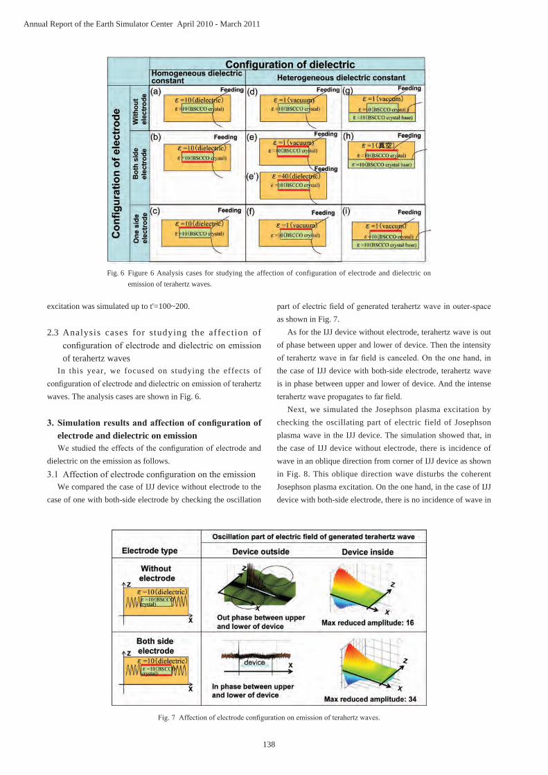
138


excitation was simulated up to t'=100~200.

2.3 Analysis cases for studying the affection of configuration of electrode and dielectric on emission of terahertz waves

In this year, we focused on studying the effects of configuration of electrode and dielectric on emission of terahertz waves. The analysis cases are shown in Fig. 6.

3. Simulationresultsandaffectionofconfigurationofelectrode and dielectric on emissionWe studied the effects of the configuration of electrode and

dielectric on the emission as follows.

3.1 Affection of electrode configuration on the emissionWe compared the case of IJJ device without electrode to the

case of one with both-side electrode by checking the oscillation

part of electric field of generated terahertz wave in outer-space as shown in Fig. 7.

As for the IJJ device without electrode, terahertz wave is out of phase between upper and lower of device. Then the intensity of terahertz wave in far field is canceled. On the one hand, in the case of IJJ device with both-side electrode, terahertz wave is in phase between upper and lower of device. And the intense terahertz wave propagates to far field.

Next, we simulated the Josephson plasma excitation by checking the oscillating part of electric field of Josephson plasma wave in the IJJ device. The simulation showed that, in the case of IJJ device without electrode, there is incidence of wave in an oblique direction from corner of IJJ device as shown in Fig. 8. This oblique direction wave disturbs the coherent Josephson plasma excitation. On the one hand, in the case of IJJ device with both-side electrode, there is no incidence of wave in

Fig. 6 Figure 6 Analysis cases for studying the affection of configuration of electrode and dielectric on emission of terahertz waves.

Fig. 7 Affection of electrode configuration on emission of terahertz waves.

139


an oblique direction from corner of IJJ device. Furthermore, we also compared the case of IJJ device with

one-side electrode to the case of one with both-side electrode as shown in Fig. 9.The simulation showed that, in the case of IJJ device with both-side electrode, the excitation of Josephson plasma excitation is stable. On the one hand, in the case of IJJ device with one-side electrode, the excitation is unstable.

From these studies, it is clear that, in electrode configuration, the type of both-side electrode IJJ device is favorable to emission of terahertz waves from the edge of IJJ device. Up to now, however, the IJJ device of one side electrode was used for the almost reported experiments because of easiness to fabricate the one side electrode device compared to both-side

one. Therefore it is summarized that the both-side electrode IJJ device is suitable to generate the intense and coherent terahertz waves.

3.2 Effects of dielectric configuration on the emissionThe case of homogeneous dielectric constant was compared

to the case of heterogeneous dielectric constant, for studying the oscillation part of electric field as shown in Fig. 10. The simulation cleared that intensity of homogeneous dielectric constant is more than that of heterogeneous dielectric constant. It indicates that increase of dielectric constant of outer space strongly contributes to the emission of terahertz waves from edge of IJJ device.

Fig. 8 Affection of electrode configuration on Josephson plasma excitation in the IJJ device.

Fig. 9 Affection of electrode configuration on Josephson plasma excitation.

Fig. 10 Affection of dielectric configuration on emission of terahertz waves.

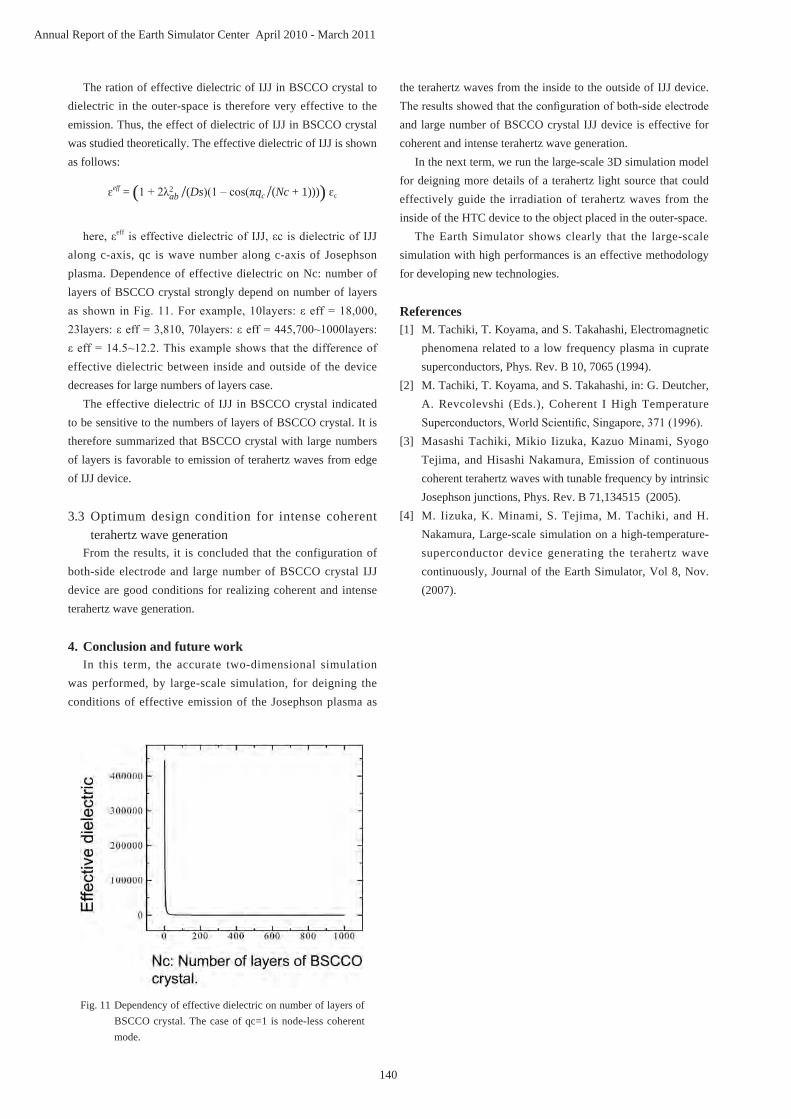
140


The ration of effective dielectric of IJJ in BSCCO crystal to dielectric in the outer-space is therefore very effective to the emission. Thus, the effect of dielectric of IJJ in BSCCO crystal was studied theoretically. The effective dielectric of IJJ is shown as follows:

ɛeff = (1 + 2λ2 /(Ds)(1 – cos(πqc /(Nc + 1)))) ɛcab

here, εeff is effective dielectric of IJJ, εc is dielectric of IJJ along c-axis, qc is wave number along c-axis of Josephson plasma. Dependence of effective dielectric on Nc: number of layers of BSCCO crystal strongly depend on number of layers as shown in Fig. 11. For example, 10layers: ε eff = 18,000, 23layers: ε eff = 3,810, 70layers: ε eff = 445,700~1000layers: ε eff = 14.5~12.2. This example shows that the difference of effective dielectric between inside and outside of the device decreases for large numbers of layers case.

The effective dielectric of IJJ in BSCCO crystal indicated to be sensitive to the numbers of layers of BSCCO crystal. It is therefore summarized that BSCCO crystal with large numbers of layers is favorable to emission of terahertz waves from edge of IJJ device.

3.3 Optimum design condition for intense coherent terahertz wave generation

From the results, it is concluded that the configuration of both-side electrode and large number of BSCCO crystal IJJ device are good conditions for realizing coherent and intense terahertz wave generation.

4. Conclusion and future workIn this term, the accurate two-dimensional simulation

was performed, by large-scale simulation, for deigning the conditions of effective emission of the Josephson plasma as

the terahertz waves from the inside to the outside of IJJ device. The results showed that the configuration of both-side electrode and large number of BSCCO crystal IJJ device is effective for coherent and intense terahertz wave generation.

In the next term, we run the large-scale 3D simulation model for deigning more details of a terahertz light source that could effectively guide the irradiation of terahertz waves from the inside of the HTC device to the object placed in the outer-space.

The Earth Simulator shows clearly that the large-scale simulation with high performances is an effective methodology for developing new technologies.

References [1] M. Tachiki, T. Koyama, and S. Takahashi, Electromagnetic

phenomena related to a low frequency plasma in cuprate superconductors, Phys. Rev. B 10, 7065 (1994).

[2] M. Tachiki, T. Koyama, and S. Takahashi, in: G. Deutcher, A. Revcolevshi (Eds.), Coherent I High Temperature Superconductors, World Scientific, Singapore, 371 (1996).

[3] Masashi Tachiki, Mikio Iizuka, Kazuo Minami, Syogo Tejima, and Hisashi Nakamura, Emission of continuous coherent terahertz waves with tunable frequency by intrinsic Josephson junctions, Phys. Rev. B 71,134515 (2005).

[4] M. Iizuka, K. Minami, S. Tejima, M. Tachiki, and H. Nakamura, Large-scale simulation on a high-temperature-superconductor device generating the terahertz wave continuously, Journal of the Earth Simulator, Vol 8, Nov. (2007).

Fig. 11 Dependency of effective dielectric on number of layers of BSCCO crystal. The case of qc=1 is node-less coherent mode.

141


テラヘルツ発振超伝導素子に関する大規模シミュレーション


飯塚　幹夫　　高度情報科学技術研究機構

著者飯塚　幹夫　　高度情報科学技術研究機構立木　　昌　　筑波大学中村　　寿　　高度情報科学技術研究機構

本研究では、電波と光の間の未利用周波数帯域にあるテラヘルツ波の応用開拓を目指し、大規模シミュレーションを利用したテラヘルツ発振超伝導素子の利用システムの設計を行なっている。テラヘルツ波は、多くの物質に対し高い透過性を持ち、生命分子を含む多くの物質と強く相互作用するため、環境、医療、物質・生命科学などへの応用が期待されている。テラヘルツ波にはパルス波と連続波とがあり、連続波はパルス波より大出力で周波数が揃うことから利用価値はパルス波よりも遥かに大きい。このため、シリコン系半導体、非線形材料等を使う連続波発振が試みられたが、未だに性能が不十分であり、新原理による連続波発振が課題であった。そこで、本研究ではわが国の独自技術としてナノスケールの高温超電導体薄膜素子を使う連続波テラヘルツ発振を目指し、地球シミュレータの大規模シミュレーションにより、これまでにその発振原理、制御法を世界で初めて明らかにした。その後、本研究を参考にしつつ発振実験が行なわれ、発振原理が実証された。これを計測システムとして実用化を目指すには、素子から発振される連続波テラヘルツ波を反射・損失・減衰を最小

限にして計測対象物に照射するための導波管の構造、形状、媒質（誘電体）などに関するシステム的な最適設計が必要となる。そのため、昨年度までに、応用計測系の基本概念を固め、素子・導波管系の連続波テラへルツ波の 3次元空間放射の非線形挙動や大出力放射のための電極形状、配置などの最適条件等を明らかにした。そこで今年度は、実用化への開発実験等を加速するため、2次元モデルで素子と誘電体配置条件や素子の元形状等とコヒーレントで強い放射との関係を明らかにした。今後は、3次元連続波テラヘルツ波の反射、減衰を考慮した素子・導波管系の大規模シミュレーションを行ない、連

続波テラヘルツ波応用の基本となるシステム概要、その設計条件を定量的に明らかにする。また、これらの計算規模はペタスケールであり、そのためのモデル拡張、並列性能向上、演算性能向上へ向けた階層メモリ利用法向上、そのためのアルゴリズムの高度化等を含めた大規模モデルの研究開発も進めていく予定である。本研究内容は大容量情報伝送やエネルギ伝送の利用研究の側面も有し、米、独、中、韓等でも類する研究が盛んであり、国際的に厳しい競争状況にある。このため、本研究では防衛的に国内特許を確保した。本研究から得られる設計情報等は、わが国の学界・産業界に優先的に提示し、日本独自の新しい産業技術の勃興に資する。

キーワード : 高温超電導体 , 素子 , テラヘルツ波生成 , 安定励起 , ジョセフソンプラズマ , HPC

143


1. Direct numerical simulations of fundamental turbulent flows

1.1 HighresolutionDNSofturbulentchannelflowIn order to study the small-scale statistics of high-Reynolds

numberwall-bounded turbulence,we performed a directnumericalsimulation(DNS)of turbulentchannelflow(TCF)of an incompressible fluid obeying the Navier-Stokes (NS) equations,inacomputationalboxwithstreamwise(x) and span-wise (z) periodicities (Lx=2πh and Lz=πh), ataReynoldsnumber Reτ =2560 based on the friction velocity uτ and the channelhalf-widthh. We achieved the sustained performance of 6.1Tflops(11.7%ofthepeakperformance)intheDNSofTCFon2048x1536x2048gridpointsusing64nodesofES2.Thenumbersofgridpointsaswellasthecomputationaldomainsizein the x and zdirectionsaretwiceaslargeasourpreviousDNS.

TheDNS isbasedon theFourier-spectralmethod inx- and z-directions,andtheChebyshev-taumethodinthewall-normaly-direction.Thealiaserrorsareremovedbythe3/2rule.TheNSequationsareexpressedintermsofthewall-normalvorticitycomponentsand theLaplacianofwall-normalvelocity.Timeadvancement is accomplished by a third-order Runge-Kutta methodfortheconvectiontermandthefirst-orderimplicitEulermethod for the viscous terms. Our DNS has been advanced up to t = 2.2 tw,wheretwisthewash-outtime.Wehavetoperformthe DNS until t > 10tw toobtainmorereliablestatistics,andtoelucidatethefiniteboxsizeeffectonthepossibleuniversalityinthe small-scale statistics.

Figure 1 shows the comparison between compensatedlongitudinal spectra E11(kx) and E33(kz) obtained in our previous DNS in the smaller domain; E11 is for the streamwise (x)

Direct Numerical Simulations of Fundamental Turbulent Flows with the World's Largest Number of Grid-points and Application to Modeling of Engineering Turbulent Flows


Yukio Kaneda GraduateSchoolofEngineering,NagoyaUniversity

Authors

Yukio KanedaTakashiIshiharaKaoruIwamotoTetsuroTamura

YasuoKawaguchiTakahiroTsukahara

GraduateSchoolofEngineering,NagoyaUniversity

GraduateSchoolofEngineering,NagoyaUniversity

MechanicalSystemsEngineering,TokyoUniversityofAgricultureandTechnology

InterdisciplinaryGraduateSchoolofScienceandEngineering,TokyoInstituteof

Technology

DepartmentofMechanicalEngineering,TokyoUniversityofScience

DepartmentofMechanicalEngineering,TokyoUniversityofScience

Weperformedhigh-resolutiondirectnumericalsimulations(DNSs)ofcanonicalturbulentflowsontheEarthSimulator2.Theyinclude(i)turbulentchannelflow,(ii)quasi-staticMHDturbulenceinanimposedmagneticfield,and(iii)turbulentboundarylayeronsinusoidalwavywalls.TheDNSsprovideinvaluabledataforthefollowingstudies,respectively;(1)thelocalanisotropyinsmall-scalestatisticsinthelog-lawlayerofturbulentchannelflow,(2)anisotropyandintermittencyofquasi-staticMHDturbulenceinanimposedmagneticfield,and(3)theeffectofthewavelengthofthesinusoidalwavywallupontheturbulentstatistics.BytheanalysisoftheDNSdata,itwasshownthat(1)thelocalanisotropydecreaseswiththedistancefromtheboundarywall,(2)themagneticfieldenhancestheintermittency,and(3)thepressuredragdecreaseswiththewavelengthofthesinusoidalwavywall.Wealsoperformedthefollowingturbulencesimulationsforenvironmentalandindustrialapplications;(i)LargeEddySimulationofturbulentboundarylayeroverhomogenousvegetationfieldusingahybridLES-RANSmodelwhichcanrepresentappropriatelyandefficiently theroughnessconditionongroundsurface,and(ii)DNSof turbulentflowsofnon-Newtoniansurfactantsolutioninachannelwithrectangularorifices.By(ii),wecouldestimatethecharacteristicsoftheheattransferassociatedwiththedragreduction.

Keywords: High-resolutionDNS, turbulentchannel flow,MHDturbulence, turbulentboundary layer, roughwall,LES,urbanturbulentboundarylayer,non-Newtonianfluid,dragreduction

144


velocity component and E33isforthespan-wise(z) component. Theclassicalvalue for theKolmogorovconstantC1 = 0.5 is alsoshown inFig.1. It is shown that there isawavenumberrangeinwhicheachspectrumisnotfarfromtheK41spectra.ThedifferencebetweenE11(kx) and E33(kz) isseeninFig.1 todecreasewiththeincreaseoftheTaylorscaleReynoldsnumberReλ (Note that Reλisafunctionofthedistancefromthewall).

1.2 DNS of quasi-static magnetohydrodynamic (MHD) turbulence

Low-magnetic-Reynolds-numbermagnetohydrodynamic(MHD)turbulenceinanimposedmagneticfieldwidelyexistsin industrialapplications,suchaselectro-magneticprocessing

of materials in metallurgical industry. When the magnetic Reynoldsnumber issufficientlysmall,wecanapply theso-calledquasi-staticapproximationtotheMHDturbulence.

Quasi-staticMHDturbulenceischaracterizedbymultiscaleanisotropy and intermittency. Wavelet representation is an efficientwaytoanalyzesuchintermittentdata,sincewaveletsarewell localized inspace, scaleanddirection.Toquantifyintermittencyinanisotropicturbulence,Boset al. [1] introduced scale- and direction-dependent statistics using three-dimensional orthonormaldiscretewavelets.

In this study,we performed high-resolutionDNSs ofincompressible quasi-staticMHD turbulence at the twointeractionparameters,i.e.N=1and3,with5123 grid points on theESandexamined theanisotropyand intermittencyof theobtainedDNSfields,usingthescale-anddirection-dependentstatistics [1].

We found that for the N=3,theimposedmagneticfieldplaysa major role on the increase of intermittency in the direction paralleltothemagneticfield.Thedetailsofthecurrentstudyareshownin[2].

2. DNS of turbulent boundary layer on rough wallsTurbulentboundarylayeronroughplatesisoneofthemost

important problems in fundamental turbulent heat transfer research,practicalengineeringapplicationsandenvironmentalprocesses.DNSof turbulentboundary layeron roughwallshasbeenbarelyperformedcomparedwith thatofotherwall-boundedturbulencesuchasturbulentchannelflows.

In this study, direct numerical simulation of turbulentboundary layerwithseveral sinusoidalwavywallshasbeenperformedinordertoinvestigatetheeffectofthewavelength

Fig.1 Comparisonbetweencompensated longitudinalspectraE11(kx) and E33(kz),aty

+=100,200,400and600intheTCFobtainedbytheDNSwith1024x1536x1024gridpointsandReτ =2560. ηisKolmogorov's lengthscale.Solidlineis theK41spectrumk5/3E(k)/ε2/3 = C1withC1 = 0.5.

Fig.2 Computationaldomainsforturbulentboundarylayeronseveralsinusoidalwavywalls.

145


ofthesinusoidalwavywall,λ,upontheturbulentstatistics.Theamplitudeof thesinusoidalwavywall,a,waskeptconstantinwallunits,andthewavelengthwasset tobea /λ=0.011,0.022and0.033.Forthespatiallydevelopingboundarylayersonsinusoidalwavywalls,weprovidedadriversectionwithaflatwallandananalysissectionwithasinusoidalwavywallasshowninFig.2.Turbulent inflowconditionsfor thedriversection are generated by rescaling the turbulent boundary layer atsomedistancedownstreamoftheinflowandbyreintroducingtherecycledmeanprofileandfluctuationfield.This techniquefollowsthoseofKongetal.[3]andLundetal.[4].Turbulentinflowconditionsfor theanalysissection,on theotherhand,aregeneratedbyexactlycopyingaturbulentfieldofthedriversection.Theparallelandvectorizationefficienciesare98.43%and99.50%,respectively.

Theaverageof thewall shearstresshardlychangeswithdecreasingthewavelength,whilstthefrictioncoefficient,whichwasdefinedasthesummationof thewallshearstressandthepressuredrag,was increasedwithdecreasingthewavelengthowingtotheincreaseofthepressuredrag(notshownhere).

3. Application of LES of turbulent flows to urban environmental and strong wind disaster problemsBasedonthefundamentalknowledgeofturbulentflows,we

extendtheLEStechniquestoatmosphericphenomenaappearingasanenvironmentalaswellasastrongwinddisasterproblemwhicharestronglyrelatedwiththehumansociety.

Firstly,LargeEddySimulation(LES)ofaturbulentboundaryflowoverhomogenousvegetationfieldwasperformedusinghybridLES-RANSmodelwhichcan representappropriatelyandefficientlytheroughnessconditionongroundsurface[5].InLESofboundarylayerflowsovervegetationfields, leavesandplantsaretoothintoresolvethembythesufficientnumberofgridpoints.So, theeffectof thoseleavesandplantsontheflowmustbe treatedwithanartificialmodel.The turbulenceclosuremodelforplantcanopyflowsusedherewasproposedbyHiraokaandOhashi[6],whichisformulatedbasedonRANS(k-ɛ) turbulencemodel.Thecomputationaldomain is2.5kmlongx0.4kmwideanditshorizontalresolutionis5mlongx2.5mwide.Thequasi-periodicboundaryconditionisemployedinstreamwisedirection(Fig.3).Theboundarylayerthicknessreachestoapproximately500mandthemeanvelocityprofile

Fig.4 Meanvelocityandturbulenceintensityprofiles.

Fig.5 Contourofstreamwisevelocity.

(a) RANS region

(b) LES region

Fig.3 Computationalregionandconceptofthequasi-periodic boundary condition for a turbulent boundarylayerflowovervegetationfield.

146


and turbulence intensity reasonably fit to those obtained by thepreviousexperimentalstudy(Fig.4). Itcanbeseen thatthe turbulence structure in LES region is very small and fine comparedtothatinRANSregion(Fig.5).

Recent architectural buildings have a variety of shapes basedonuniquedesignerconcepts,and thecurvedsurfacesare frequentlyusedforbuildingwall.Here,asa typicalanda fundamentalcase in suchbuildings,acircularcylinder isfocusedon.Theflowcharacteristicsaroundacircularcylinderin realistic high Reynolds number region are investigated by use oftheLESmodel.Asaresult,thepresentLESmodelsucceededin accurately simulating the drastic change of aerodynamic coefficient (Fig.6).Also,detailsof the flowstructuresnearseparatingandreattachingregionareclarifiedbyvisualizationofthecomputeddata(Fig.7).

4. DNS of the turbulence in non-Newtonian surfactant solutionTheeffectofpolymerorsurfactantadditiveson turbulent

flowhas receivedmuch attention frombothpractical andscientificperspectivessincethediscoveryinthe1940s,thatis,small additive concentration can lead to significant reduction indragof50%orgreater[7].Thisphenomenonisofpracticalimportance and has recently been implemented in several industrialsystemstosaveenergy.Ingeneral, thesolutionusedasaworkingfluidforsuchadrag-reducingflowisaviscoelastic(non-Newtonian) liquid.Thepropertiesof the liquidsolutionmeasuredeveninsimpleshearorextensionalflowsareknowntoexhibitappreciablydifferentfromthoseofthepuresolvent.Thegoalofthepresentworkistobetterunderstandthephysicsofviscoelastic turbulent flow,particularly in thecontextofcomplicatedflowgeometry.

ManyDNS of polymer-induced drag reductionwereperformed for various types of canonical flows, such as

Fig.6 Drasticchange indragcoefficientat theveryhighReynolds numbers.

Fig.7 Three-dimensional flow structures nearseparating and reattaching region.

Fig.8 Instantaneousflowandthermalfieldinviscoelasticturbulentflowthrougharectangularrib (at x=0with0.1δ thickness):green isosurface,vortex identifiedby thesecondinvariantofstraintensor;contours, temperatureorwallheatflux.Thermalboundaryconditionistheconstanttemperaturedifferencebetweentwowalls(y=0and2δ),theperiodic condition is applied in x and z.

Fig.9 LocalNusselt-numberprofile as afunction of x, fordifferentPrandtlnumbers.Alsoshownareestimatedvalues in the case of a smooth channel at the same bulk Reynolds number.

147


isotropicturbulence,shear-driventurbulence,channelflow,andboundarylayer.Althoughflowsthroughcomplicatedgeometrieshave been studied by a number of researchers for the laminar regimeforbothNewtonianandviscoelastic fluids [8], thoseunder turbulentconditionshavereceivedmuchlessattention,exceptthatMakinoet al. [9]carriedoutDNSoftheturbulent'Newtonian'flowinachannelwithperiodicrectangularorifices.Further,itshouldbenotedthat,totheauthors'knowledge,therehasneverbeenanyDNSofturbulentviscoelasticflowwiththeorifice partly due to the Hadamard instability in viscoelastic-flowcalculations[10].Inthepresentstudy,weexecutedDNSofaviscoelasticfluidinthesamegeometrywiththatofMakinoet al. [9],usingacompositeflux-limiter(minmod)schemetothe convective term in the Giesekus-model constitutive equation andapplyingfinergridsrelativetoexistingsimilarworks.

Majordifferencesbetweenthepresentstudyandpublishedworks on smooth channels are related to the streamwisevariationoftheflowstateandthemainareaswhereturbulenceisproduced.Therefore,theinstantaneousvortexstructuresandtherelevantmomentumandheattransportswithinthestrongshearlayerjustdownstreamoftheorificewillbeexplored.Figure8presentsaninstantaneoussnapshotofeddies,withemphasisontheorificedownstream,andsurfacedistributionsoftemperatureandwallheatflux,revealinghighheatfluxesonthewallsurfaceunderthevortexmotions.It is interestingtonotethatthewallheat fluxalsobecomes intermittentlyhigh fardownstreamoftheorifice,namely,atx=8-10,wherenoapparenteddyisobserved. Such heat-transfer enhancement leads to an increase oflocalNusseltnumbercomparedwiththeNewtoniancase,ascanbeseeninFig.9.Therefore,wedrawaconclusionthatthisgeometrygives rise to thedissimilaritybetweenmomentumand heat transports and the advantage of the heat transfer comparedwiththesmoothchannel.However,thepresentbulkReynolds number (Rem~1200)wasconsiderably lower thanthosecorrespondingconditionsunderwhichdragreductioninpracticalflowsystemsisobservedwithdiluteadditivesolutions.It isnecessarytofurthercalculateviscoelasticflowsathigherReynolds numbers andwith awide range of rheologicalproperties.

References[1] W.Bos,L.Liechtenstein,andK.Schneider,"Directional

and sca le -dependen t s t a t i s t i c s o f quas i - s t a t i c magnetohydrodynamic turbulence,"Phys.Rev.E76,046310,2007.

[2] N.Okamoto,K.Yoshimatsu,K.Schneider,andM.Farge,"Directionalandscale-dependentstatisticsofquasi-staticmagnetohydrodynamicturbulence,"ESAIM:Proceedings(accepted).

[3] Kong,H.,Choi,H., andLee, J.S., "Directnumericalsimulationof turbulent thermalboundary layers,"Phys.Fluids,12,2666,2000.

[4] Lund,T.S.,Wu,X.,andSquires,K.D.,"Generationofturbulent inflowdataforspatially-developingboundarylayersimulations,"J.Comput.Phys.,140(2),1998,233-258.

[5] F.Hamba,"AHybridRANS/LESSimulationofTurbulentChannelFlow,"Theoret.Comput.FluidDynamics,16,387-403,2003.

[6] H.HiraokaandM.Ohashi, "Ak-ɛ turbulenceclosuremodelforplantcanopyflows,"Proc.ofthe4thInt.Symp.onComp.WindEng.,693-696,2006.

[7] A.Gyr andH.W.Bewersdorff,Drag reduction of turbulent flows by additives,KluwerAcademicPublisher,Dordrecht,Netherlands,1995.

[8] P.J.Oliveira,"Asymmetric flowsofviscoelastic fluidsin symmetric planar expansiongeometries," J.Non-NewtonianFluidMech.,114,33-63,2003.

[9] S.Makino,K. Iwamoto,andH.Kawamura,"Turbulentstructuresandstatistics in turbulentchannel flowwithtwo-dimensionalslits,"Int.J.Heat&FluidFlow,29,602-611,2008.

[10] D.D. Joseph,Fluid dynamics of viscoelastic liquids,Springer-Verlag,NewYork.,1990.

148


乱流の世界最大規模直接数値計算とモデリングによる応用計算


金田　行雄　　名古屋大学　大学院工学研究科

著者金田　行雄　　名古屋大学　大学院工学研究科石原　　卓　　名古屋大学　大学院工学研究科

岩本　　薫　　東京農工大学　工学府

田村　哲郎　　東京工業大学　大学院総合理工学研究科川口　靖夫　　東京理科大学　理工学部

塚原　隆裕　　東京理科大学　理工学部

地球シミュレータ（ES2）を用いて、乱流の規範的（カノニカル）な問題の大規模直接数値計算（DNS）を実施した。具体的には（i）世界最大レイノルズ数の平行平板間乱流（ii）磁場中の準定常 MHD 乱流、（iii）正弦波状壁面上の乱流境界層の DNS である。これらの DNS は各々、（1）高レイノルズ数壁乱流の対数領域における局所非等方性、（2）磁場中の準定常 MHD 乱流における非等方性と間欠性、（3）正弦波状壁面の波長が乱流等計量に与える影響、について研究するための貴重なデータを提供するものである。データ解析により、（1）局所的な非等方性が壁から離れるに従って小さくなること、（2）磁場が MHD 乱流場中の間欠性を強める働きがあること、（3）正弦波の波長が小さくなるに従い圧力抵抗が増加することを見いだした。

我々はまた、これまでに得られた乱流統計の基礎的な知見に基づき、環境や工業的な応用問題として、以下の大規模数値計算を実施した。具体的には、（i）適切かつ有効に粗面の条件を与えることが可能な LES と RANS のハイブリッドモデルを用いた計算により、一様な植生上で発達する乱流境界層の非定常解析を行った。また、（ii）直方体型のオリフィスのあるチャネル中の非ニュートン流体の乱流の DNS により、抵抗低減に伴う熱伝達率特性の評価に成功した。

キーワード : 大規模直接数値計算 , 平行二平板間乱流 , MHD乱流 , 乱流境界層 , 粗面 , LES, 都市型大気乱流境界層 , 界面活性剤 , 抵抗低減

149


1. IntroductionMore than 99% of microorganisms inhabiting natural

environments are difficult to culture under laboratory conditions. While genomes of the unculturable organisms have remained primarily uncharacterized, these should contain a wide range of novel genes of scientific and industrial interest. To explore such an enormous quantity of novel genome resources, metagenomic analyses, which are culture-independent approaches performing shotgun sequencing on mixed genome DNA samples, have been developed, and vast numbers of fragment sequences have been deposited in the International Nucleotide Sequence Databases (INSD). The metagenomic sequencing is undoubtedly a powerful strategy for comprehensive study of a microbial community in an ecosystem, but for most of the sequences, it is difficult to predict from what phylotypes each sequence is derived. This is because orthologous sequence sets, which cover a broad phylogenetic range needed for constructing reliable phylogenetic trees through sequence homology searches, are unavailable for novel gene sequences. G plus C percentage (%GC) has long been used as a fundamental parameter for phylogenetic classification of microorganisms, but the %GC is apparently too simple a parameter to differentiate a wide variety of species. Oligonucleotide composition, however, can be used even to distinguish species with the same %GC,

because oligonucleotide composition varies significantly among microbial genomes and thus are called "genome signature". Phylogenetic clustering and classification in the present study is designed as an extension of the single parameter "%GC" to the multiple parameters "oligonucleotide frequencies".

We previously modified the SOM developed by Kohonen's group [1-3] for genome informatics on the basis of batch-learning SOM (BLSOM), which makes the learning process and resulting map independent of the order of data input [4-6]. The BLSOM thus developed could recognize phylotype-specific characteristics of oligonucleotide frequencies in a wide range of genomes and permitted clustering (self-organization) of genomic fragments according to phylotypes with neither the orthologous sequence set nor the troublesome and potentially mistakable processes of sequence alignment. Furthermore, the BLSOM was suitable for actualizing high-performance parallel-computing with the high-performance supercomputer "the Earth Simulator", and permitted clustering (self-organization) of almost all genomic sequences available in the International DNA Databanks on a single map [7-9]. By focusing on the frequencies of oligonucleotides (e.g., tetranucleotides), the BLSOM allowed highly accurate classification (self-organization) of most genomic sequence fragments on a species basis without providing species-related

A Large-scale Genomics and Proteomics Analyses Conducted by the Earth Simulator


Toshimichi Ikemura Nagahama Institute of Bio-Science and Technology

Authors

Takashi Abe*1, Hiroshi Uehara*1, Yuki Iwasaki*1, Kennosuke Wada*1 and Toshimichi Ikemura*1

*1 Nagahama Institute of Bio-Science and Technology

Although remarkable progress in metagenomic sequencing of various environmental samples icluding those from oceans has been made, large numbers of fragment sequences have been registered in DNA databanks without information on gene function and phylotype, and thus with limited usefulness. Scientific and industrial useful activity is often carried out by a set of genes, such as those constituting an operon. In this connection, metagenomic approaches have a weakness because sets of the genes are usually split up, since the sequences obtained by metagenome analyses are fragmented into short segments. Therefore, even when a set of genes responsible for a scientifically and/or industrially useful function is found in one metagenome library, it is difficult to know whether a single genome harbors the entire gene set or whether different genomes have individual genes. By modifying Self-Organizing Map (SOM), we previously developed BLSOM for oligonucleotide composition, which allowed self-organization of sequences according to genomes. Because BLSOM could reassociate genomic fragments according to genome, BLSOM should ameliorate the abovementioned weakness of metagenome analyses. Here, we developed a strategy for clustering of metagenomic sequences according to phylotypes and genomes, by testing a gene set for a metabolic pathway contributing to environment preservation.

Keywords: batch learning SOM, oligonucleotide frequency, protein function, metagenomics

150


information during BLSOM computation. Therefore, the present unsupervised and alignment-free clustering method should be most suitable for phylogenetic clustering of sequences from novel unknown organisms [10-12]. We have employed BLSOM for metagenomic studies on a large amount of environmental sequences, in joint research with experimental research groups analyzing various environmental and clinical samples [10,11].

Biological activity with industrial usefulness, such as processes responsible for environmental clean-up and preservation, is often carried out by a set of genes rather than a single gene; e.g., an operon responsible for one metabolic activity. However, in the case of metagenomic approaches, contigs with a significant length, such as those covering an operon, were obtained only for very dominant species after assembling of sequences. Even when a set of genes responsible for an industrially useful function is found in one metagenome library, it is difficult to know whether a single genome has the gene set of interest or whether different genomes coexisting in the sample have individual genes. From the industrial and scientific view, it is valuable to find a metagenomic library that may have a single genome having a full set or, at least, a major portion of the gene set. In the present report, we explained a strategy for the in-silico association of fragmented sequences according to phylotype (hopefully even to species), by focusing on a set of genes contributing to environmental cleanup and preservation.

2. MethodsGenomic fragment sequences derived from metagenome

analyses were obtained from http://www.ncbi.nlm.nih.gov/GenBank/. Metagenome sequences shorter than 1 kb in length were not included in the present study. When the number of undetermined nucleotides (Ns) in a sequence exceeded 10% of the window size, the sequence was omitted from the BLSOM analysis. When the number of Ns was less than 10%, the oligonucleotide frequencies were normalized to the length without Ns and included in the BLSOM analysis. Sequences that were longer than a window size were segmented into the window size, and the residual sequences, which were shorter than the window size, were omitted from the BLSOM analysis.

BLSOM learning was conducted as described previously [4-6], and the BLSOM program was obtained from UNTROD Inc. ([email protected]).

3. Results3.1 BLSOMs for sequences obtained by metagenome

analysesTo test the clustering power of BLSOM for oligonucleotide

composition in metagenomic sequences, we analyzed a large quantity of fragment sequences obtained from eight typical metagenomic libraries currently available; for details about metagenomic libraries, refer to [12]. To develop an informatics strategy useful to search gene candidates contributing to environmental cleanup and preservation, we focused on

Fig. 1 DegeTetra-BLSOM for 1-kb metagenomic sequences of 8 environmental samples. Lattice points that include sequences from more than one environmental sample are indicated in black, and those containing sequences only from one sample are indicated in color as follows: Brisbane Active Sludge (■), Madison Active Sludge (■), Washington Lake (■), Hawaii Ocean (■), Whale Bones (■), Minnesota Farm Land (■), Human Guts (■), and Richmond Mine (■). In eight panels with the sample names above the panels, all lattice points containing sequences from one sample are indicated in a color representing the sample, regardless of coexistence of sequences from other samples.

151


metagenomic sequences longer than 1 kb, which likely harbored an intact protein-coding sequence. In DNA databases, only one strand of a pair of complementary sequences is registered. Some sequences represent the coding sequences of the protein-coding genes, but others represent the template sequences. These two types of sequences have somewhat different characteristics of oligonucleotide composition, resulting in the split of the species-specific territory into at least two separate territories, which primarily reflect a transcriptional polarity for individual genes [6]. When we constructed BLSOM in which the frequencies of a pair of complementary oligonucleotides (e.g., AACC and GGTT) in each fragment were summed, the tendency of the splitting into a few territories was diminished for most of species [7]. For phylogenetic clustering of metagenomic sequences, it is unnecessary to know the transcriptional polarity for the sequence, and the split into a few territories complicates the clustering according to genome. Therefore, in the present study, we constructed BLSOMs for the degenerate sets of tri- and tetranucleotides: DegeTri- and DegeTetra-BLSOMs, respectively.

The result of DegeTetra-BLSOM for 1- or 2-kb sequence fragments (i.e., a window size of 1 or 2 kb) was listed in Figs. 1 or 2, respectively; DegeTri-BLSOM gave a similar result [12]. Sequences longer than 2 kb (approximately 15% of the sequences longer than 1 kb) should represent contig sequences obtained by the assembling process of shot-gun sequencing, and therefore, primarily represent sequences derived from dominant or subdominant species in each environment. In other words, BLSOMs constructed with the 2-kb sequences is suitable for determining the characteristics of dominant and

subdominant species in the environment. In the "All" panel in Figs. 1 and 2, lattice points that contained sequences from one environment are indicated by the color representing that environment, and those that included sequences from more than one environment are indicated in black. In each of other eight panels in Figs. 1 and 2, all lattice points containing sequences derived from one environment were indicated by the color representing that environment. Difference in characteristics of individual environmental samples could be visualized on a single plane, supporting efficient knowledge discovery from a large number of metagenomic sequences and thus showing a powerful function of BLSOM. The observation that DegeTri- and DegeTetra-BLSOMs gave similar results showed that the separation patterns should represent basal characteristics of the environmental samples. On the two BLSOMs listed in Figs. 1 and 2, global patterns of the two sludge samples (Brisbane and Madison Sludge panels) resembled each other, but there were clear compact zones that were specifically found only in one sludge sample. Since the compact zones were colored in red or pink even in the "All" panel, the sequences were derived presumably from characteristic species in the environment, rather than the species ubiquitously present in various environments.

Visualization power of BLSOM could support this kind of efficient and luminous knowledge discovery. The pattern of the Washington Lake was much simpler on both BLSOMs than that of the Hawaii Ocean. A few large but isolated territories were observed in the Washington Lake, indicating that microorganisms with close phylogenetic relations may dominate in the sample. Sequences derived from the Whale

Fig. 2 DegeTetra-BLSOM for 2-kb metagenomic sequences of 8 environmental samples. Lattice points are indicated in color as described in Fig. 1.

152


Bones or the Minnesota Farm Land were distributed widely on the 1-kb BLSOM, but were much localized on the 2-kb BLSOM. This indicated that these samples contained a wide variety of genomes but phylotypes of dominant species were rather limited. In the case of the Human Guts, the patterns were very complex both on 1- and 2-kb BLSOMs. This showed a high complexity of genomes present in this sample, which was a mixture of gut samples from 13 different Japanese individuals. There were wide green zones that were primarily composed of sequences derived from Human Guts (green zones in ALL panels in Figs. 1 and 2), indicating that the microbial community in the human body environment differed significantly from that of natural environments.

3.2 Reassociation of genomic fragments according to phylotypes and genomes

The pattern of sequences derived from an acid mine drainage at the Richmond Mine was very simple ("Richmond Mine" in Figs. 1 and 2). Tyson et al. [13] selected acidophilic biofilms in this acid mine drainage for metagenome shotgun-sequencing because of the low-complexity of constituent genomes. They attempted to reconstruct dominant genomes by assembling a large number of sequences obtained with the shotgun sequencing, and actually, reconstructed one nearly complete genome of Leptospirillum group II, and many scaffold sequences for Ferroplasma type II [13]. In the "Richmond Mine" panel of 2-kb DegeTetra BLSOMs (Fig. 2), there were two major compact territories: one was quite compact (A territory) but the other was rather extended (B territory). To examine the sequences present in these territories, a BLAST search of each sequence in A or B territory against NCBI RefSeq (non-redundant database of sequences) was conducted. More than 99% of sequences from the compact A territory were assigned to the sequences from Leptospirillum, but a major portion of the sequences in the extended B territory showed the highest similarity to sequences from Ferroplasma. This finding obtained by BLSOM supported the view that BLSOM has a potentiality for reassociating genomic fragments in a metagenome library according to genome, even in the presence of a massive quantity of sequences derived from a wide variety of genomes.

For the case of environmental sequences with a low genome complexity such as those from biofilms in the acid mine, reassociation of the metagenomic sequences according to genome can be obtained for a dominant species, by constructing one complete genome after sequence-assembling with conventional sequence homology searches. This reassociation, however, becomes increasingly difficult, when subdominant or minor populations are concerned. If a completely-sequenced genome with a very close phylogenetic relationship is available, contigs of metagenomic sequences even derived from a subdominant species may be mapped on the template genome and thus classified according to genome. However, a good

template genome would not be available for novel, poorly-characterized phylogenetic groups. Because one main purpose of metagenome analyses was to find novel species in environments, the method that inevitably dependents on a template genome is apparently inappropriate. In the case of BLSOM, reassociation (self-organization) of genomic fragments according to genome can be attained without the template genome, showing its wide applicability.

3.3 Genes contributing to environmental preservationMetagenome approaches should allow extensive surveys

of sequences useful in scientific and industrial applications. Biological activity with industrial usefulness is often carried out by a set of genes rather than a single gene, such as those constituting an operon. However, contigs with a significant length, e.g., those covering an operon, could not be obtained, except in the case of very dominant species. Therefore, even when a set of genes of interest is found in an environmental sample with sequence homology searches, it is difficult to know whether a single genome has a set of the genes or different genomes in the sample happen to have these genes as a whole. From the industrial and scientific view, the former case, especially representing novel genome, should be valuable, and a bioinformatics strategy to distinguish the two cases becomes important for effectively utilizing metagenomic sequences. Because BLSOM have a potentiality to reassociate fragmental sequences according to genome, it may distinguish the two cases and thus ameliorate a weakness of the metagenome approaches. To test a feasibility of the abovementioned informatics strategy, we searched gene candidates useful for environmental preservation such as degradation of hazardous compounds. As a model case, we chose a set of ten genes, which are responsible for the metabolic activity of PCB degradation: bphA1, A2, A3, A4, B, C, D, E, F, and G. Using amino-acid sequences of the ten enzymes as queries, we searched the candidate genes of interest from the present metagenomic sequences derived from the eight environmental samples, with the DDBJ-tBLASTn search under a strict criterion (e values less than 1e-20); for details, refer to [12]. Candidate genes representing nine and eight out of the ten enzyme genes were found in the Washington Lake and Hawaii Ocean samples, respectively. It should be mentioned here that a full set of the gene candidates of interest was not found in any environmental samples analyzed here. This might indicate the absence of genomes having a full set of the genes in these environments. In usual metagenomic data, however, a coverage density by fragmental sequences may not reach to a level that completely covers a certain genome. In a practical experimental approach, the first trial may be a search for genome resources to cover a significant portion of the metabolic pathway of interest, by analyzing various environmental samples. If a significant portion of the pathway genes is found in a certain environmental sample, a larger scale of metagenomic sequencing, which

153


may completely cover the possible candidate genome, will be conducted on the environmental sample. A purpose of the present study was to develop an informatics strategy, rather than an actual search for the PCB-degradation pathway, and therefore, we focused on the two environmental samples (Washington Lake and Hawaii Ocean samples) having a major part of the degradation pathway.

We next identified lattice points, on which the metagenomic sequences having the gene candidates for the PCB-degradation pathway were mapped, by finding the lattice point that had the minimum Euclidean distance in the multidimensional space for each candidate sequence. Lattices points containing the candidate gene sequences were widely scattered in the Washington Lake sample (Fig. 3A), indicating that the candidate sequences were presumably derived from various genomes. In contrast, in the Hawaii Ocean, sequences of gene candidates were located in a restricted zone (marked by a circle in Fig. 3B) and covered seven genes out of the initial eight genes, showing a powerful function of BLSOM for identifying potentially useful genome resources. In the "All" panel in Figs. 1 and 2, the compact territory in the Hawaii Ocean (marked by a circle in Fig. 3B) was colored in brownish yellow, showing that the sequences present in this territory were derived from the species specifically present in the Hawaii Ocean, rather than those present in ubiquitous environments.

4. Discussion and PerspectiveWe established a method for identifying potentially useful

genome resources from environments. It should be mentioned here that the resolving power for individual species on BLSOM in Figs. 1 and 2 was inevitably dependent on the metagenomic sequences included in the analysis, and the compact territory specific to the Hawaii Ocean might be composed of closely

related, multiple genomes. We have recently developed a wide applicable strategy, which could separate metagenomic sequences present in one compact territory (e.g., that found in the Hawaii Ocean) according to phylotypes and hopefully to species, without effects of other metagenomic sequences coexisting [12]. In the strategy, random sequences with nearly the same mono-, di- or trinucleotide composition to each metagenomic sequence in the compact territory were generated [14]. Then, we constructed DegeTetra-BLSOM for the metagenomic sequences plus the random sequences. In the presence of the random sequences, two major compact territories, a few small territories and many scattered points were separately observed, which were surrounded by random sequences [12]. In one of the major territory, a major portion of PCB-degradation pathway genes was found, showing the usefulness of the strategy to specify a genome resource that should have a major portion (if not all) of the metabolic pathway genes.

Concerning a set of genes responsible for a certain metabolic pathway derived from one genome, homology search methods can provide information only if a very large amount of metagenomic sequences is available for constructing a nearly complete genome by their assembling or if there is a template genome sequence that is derived from a closely related species with the respective environmental one and thus is usable for mapping of metagenomic sequences. In contrast, the present in-silico association with BLSOM can be achieved without a template genome for mapping and thus is applicable to the really novel, environmental genomes.

AcknowledgementsThis work was supported by Grant-in-Aid for Scientific

Research (C, 20510194) and for Young Scientists (B, 20700273)

Fig. 3 Lattice points containing sequences harboring gene candidates for PCB-degradation pathway. (A), (B): 2-kb DegeTetra-BLSOM for Washington Lake or Hawaii Ocean listed in Fig. 2, respectively. In the right-side panel, lattice points containing sequences harboring the gene candidate sequences were indicated by dots. A compact territory in the Hawaii Ocean containing a cluster of gene candidate sequences was marked with a circle.

154


from the Ministry of Education, Culture, Sports, Science and Technology of Japan. The present computation was done with the Earth Simulator of Japan Agency for Marine-Earth Science and Technology.

References [1] T. Kohonen, "The self-organizing map", Proceedings of

the IEEE, vol. 78, pp. 1464-1480, 1990.[2] T. Kohonen, E. Oja, O. Simula, A. Visa, and J. Kangas.

"Engineering applications of the self-organizing map", Proceedings of the IEEE, vol. 84, pp. 1358-1384, 1996.

[3] T. Kohonen, Self-Organizing Maps. Berlin, Springer, 1997.

[4] S. Kanaya, M. Kinouchi, T. Abe, Y. Kudo, Y. Yamada, T. Nishi, H. Mori, and T. Ikemura, "Analysis of codon usage diversity of bacterial genes with a self-organizing map (SOM): characterization of horizontally transferred genes with emphasis on the E. coli O157 genome", Gene, vol. 276, pp.89-99, 2001.

[5] T. Abe, S. Kanaya, M. Kinouchi, Y. Ichiba, T. Kozuki, and T. Ikemura, "A novel bioinformatic strategy for unveiling hidden genome signatures of eukaryotes: self-organizing map of oligonucleotide frequency", Genome Inform., vol. 13, pp. 12-20, 2002.

[6] T. Abe, S. Kanaya, M. Kinouchi, Y. Ichiba, T. Kozuki, and T. Ikemura, "Informatics for unveiling hidden genome signatures", Genome Res., vol. 13, pp. 693-702, 2003.

[7] T. Abe, H. Sugawara, M. Kinouchi, S. Kanaya, and T. Ikemura, "Novel phylogenetic studies of genomic sequence fragments derived from uncultured microbe mixtures in environmental and clinical samples", DNA Res., vol. 12, pp. 281-290, 2005.

[8] T. Abe, H. Sugawara, S. Kanaya, M. Kinouchi, and T. Ikemura, "Self-Organizing Map (SOM) unveils and visualizes hidden sequence characteristics of a wide range of eukaryote genomes", Gene, vol. 365, pp. 27-34, 2006.

[9] T. Abe, H. Sugawara, S. Kanaya, and T. Ikemura, "Sequences from almost all prokaryotic, eukaryotic, and viral genomes available could be classified according to genomes on a large-scale Self-Organizing Map constructed with the Earth Simulator", Journal of the Earth Simulator, vol. 6, pp.17-23, 2006.

[10] T. Uchiyama, T. Abe, T. Ikemura, and K. Watanabe, "Substrate-induced gene-expression screening of environmental metagenome libraries for isolation of catabolic genes", Nature Biotech., vol. 23, pp. 88-93, 2005.

[11] H. Hayashi, T. Abe, M. Sakamoto, H. Ohara, T. Ikemura, K. Sakka, and Y. Benno, "Direct cloning of genes encoding novel xylanases from human gut ", Can. J. Microbiol., vol. 51, pp. 251-259, 2005.

[12] H. Uehara, Y. Iwasaki, C. Wada, T. Ikemura, and T. Abe, "A novel bioinformatics strategy for searching industrially useful genome resources from metagenomic sequence libraries", Genes Genet. Sys., vol. 86, pp. 53-66, 2011.

[13] G.W. Tyson, J . Chapman, P . Hugenhol tz , E.E. Allen et al, "Community structure and metabolism through reconstruction of microbial genomes from the environment", Nature, vol. 428, pp. 37-43, 2004.

[14] T. Abe, K. Wada, Y. Iwasaki, and T. Ikemura, "Novel bioinformatics for inter- and intraspecies comparison of genome signatures in plant genomes", Plant Biotechnology, vol. 26, pp. 469-477, 2009.

155


ESを用いた大規模ゲノム・プロテオミクス解析：多様な環境由来の大量メタゲノム配列から、重要な代謝経路を保持する有用ゲノム資源を探索する新規戦略


池村　淑道　　長浜バイオ大学　バイオサイエンス学部

著者阿部　貴志 *1，上原　啓史 *1，岩崎　裕基 *1，和田健之介 *1，池村　淑道 *1

*1 長浜バイオ大学　バイオサイエンス学部

海洋を代表例とする、多様な地球環境で生育する微生物類は培養が困難なため膨大なゲノム資源が未開拓・未利用に残されてきた。環境中の生物群集から培養せずにゲノム混合物を回収し、断片ゲノム配列を解読し有用遺伝子を探索する「メタゲノム解析法」が開発され、科学的・産業的に注目を集めている。我々が開発した一括学習型自己組織化マップ法（BLSOM）は、断片ゲノム配列を生物種ごとに高精度に分離（自己組織化）する能力を持つ。既知の全生物種由来のゲノム断片配列を一枚の BLSOM上で俯瞰し、特徴抽出をする事も可能である。国際 DNAデータベースに収録されている、代表的な 8環境由来の混合ゲノム試料に関しての、大規模メタゲノム解

析で得られた大量塩基断片配列を対象に、3連並びに 4連塩基頻度の BLSOM解析を行った所、各環境に特異的に存在するゲノム類に由来する配列を特定出来た。メタゲノム解析では、一つの代謝系を構成する酵素群の遺伝子が、オペロンを構成して近傍に位置していても、断片配列の解読の過程で、泣き別れを起こしてしまう。BLSOMはこれらの泣き別れを起こした配列を、in silicoで再集合させる能力を持つ。環境汚染物質の分解に関与する代謝系を構成する酵素群（例えば、PCB分解に関与する 10酵素）をモデル系として、その大半を持つゲノムを探索する目的の BLSOM法を確立した。広範囲のゲノムが解読された結果、アミノ酸配列の相同性検索では機能が推定できない、機能未知なタンパク質が大

量に蓄積し、産業的にも未利用なまま残されてきた。オリゴペプチド頻度の BLSOMを用いれば、これらの大量なタンパク質類の機能推定が可能である。

キーワード : 自己組織化マップ , BLSOM, 環境微生物 , オリゴヌクレオチド , 環境浄化 , メタゲノム解析

157


1. IntroductionPlasticity in BCC metals is mainly mediated by thermal

activation of kink-pair nucleation in screw dislocation lines which are required to overcome strong lattice friction, and shows strong dependence on the direction of the applied stress and temperature [1]. Therefore it is crucial to estimate the lattice friction of a dislocation from atomistic calculations to model plasticity in BCC metals. The Peierls potential which causes lattice friction in BCC iron has been calculated using the density functional theory (DFT) with localized basis [2] [3]. In the present work we employ more accurate plane-wave basis DFT to calculate Peierls potential of an isolated screw dislocation core to obtain more reliable estimate.

2. Computational methodThe effect of long-range strain field generated by a

dislocation is incorporated into calculation using the so-called flexible boundary condition [4]. The system is divided into three concentric hexagonal regions 1, 2, and 3 as shown in Fig. 1. First, region 1 and 2 are used in DFT calculations and atoms in region 1 are relaxed to account for non-linear forces around a core, while atoms in region 2 are fixed. After the DFT relaxation, region 1, 2, and 3 are used in the second step where atoms in region 2 and 3 are relaxed according to linear elastic forces. These steps are repeated alternately until convergence. The number of atoms in region 1 and 2 is 48 and 99, respectively.

The electronic structure calculations and the structure relaxations by force minimizations in DFT steps are performed

using Vienna Ab initio Simulation Package (VASP) with Projector Augmented Wave (PAW) method and ultrasoft pseudopotentials. The exchange correlation energy is calculated by generalized gradient approximation (GGA). In all cases, spin-polarized calculations are employed. Monkhorst Pack k-point of 1x1x24 mesh is used, and convergence of Peierls barrier energy with respect to the increasing mesh number at 1x1x24 is confirmed. The Methfessel-Paxton smearing method with 0.1-eV width is used. The cutoff energy for the plane wave basis set is 400 eV. Structural relaxation is terminated when maximum force acting on movable degree of freedom becomes less than 0.01eV/Angstrom.

In the present work we investigate two-dimensional energy landscape of Peierls potential which determines the mobility and migration path of a screw dislocation. To investigate two-dimensional energy landscape, we use the drag method in which displacements of three atoms around the screw dislocation core are fixed in the Burger's vector direction to control the dislocation position. All other atoms in region 1 are relaxed in the DFT calculations, and the energy of a relaxed configuration gives Peierls potential at the dislocation position.

Note that the same boundary condition must be used for each dislocation position to calculate an energy difference between them. Since the flexible boundary condition is optimized for the easy-core position, other dislocation configurations have excess energy which comes from incompatibility between the core region and the boundary region. This excess energy mostly consists of linear elastic energy which can be easily calculated without DFT calculations. This elastic excess energy

First-principles Calculation on Peierls Potential of an Isolated Screw Dislocation in BCC Iron


Hideo Kaburaki Japan Atomic Energy Agency

Authors

Mitsuhiro Itakura*1, Hideo Kaburaki*1, Masatake Yamaguchi*1, Tatsuro Endo*1, Kenji Higuchi*1, Shigenobu Ogata*2 and Hajime Kimizuka*2

*1 Japan Atomic Energy Agency

*2 Osaka University

Peierls potential of an isolated screw dislocation in BCC iron is calculated using first-principles method. We have found that the Peierls barrier is 0.04 eV per Burger's vector, and that the two dimensional Peierls potential around a hard-core position is nearly flat. These results significantly differ from currently available molecular dynamics potentials, and indicate that improved molecular dynamics potential is necessary for the simulations of plastic deformation.

Keywords: first-principles calculation, screw dislocation, Peierls potential, BCC iron.

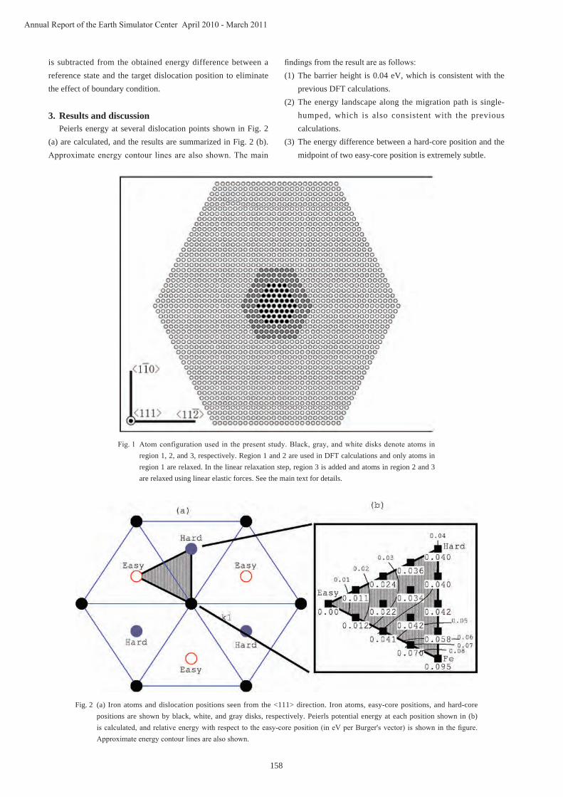
158


is subtracted from the obtained energy difference between a reference state and the target dislocation position to eliminate the effect of boundary condition.

3. Results and discussionPeierls energy at several dislocation points shown in Fig. 2

(a) are calculated, and the results are summarized in Fig. 2 (b). Approximate energy contour lines are also shown. The main

findings from the result are as follows:(1) The barrier height is 0.04 eV, which is consistent with the

previous DFT calculations.(2) The energy landscape along the migration path is single-

humped, which is also consistent with the previous calculations.

(3) The energy difference between a hard-core position and the midpoint of two easy-core position is extremely subtle.

Fig. 1 Atom configuration used in the present study. Black, gray, and white disks denote atoms in region 1, 2, and 3, respectively. Region 1 and 2 are used in DFT calculations and only atoms in region 1 are relaxed. In the linear relaxation step, region 3 is added and atoms in region 2 and 3 are relaxed using linear elastic forces. See the main text for details.

Fig. 2 (a) Iron atoms and dislocation positions seen from the <111> direction. Iron atoms, easy-core positions, and hard-core positions are shown by black, white, and gray disks, respectively. Peierls potential energy at each position shown in (b) is calculated, and relative energy with respect to the easy-core position (in eV per Burger's vector) is shown in the figure. Approximate energy contour lines are also shown.

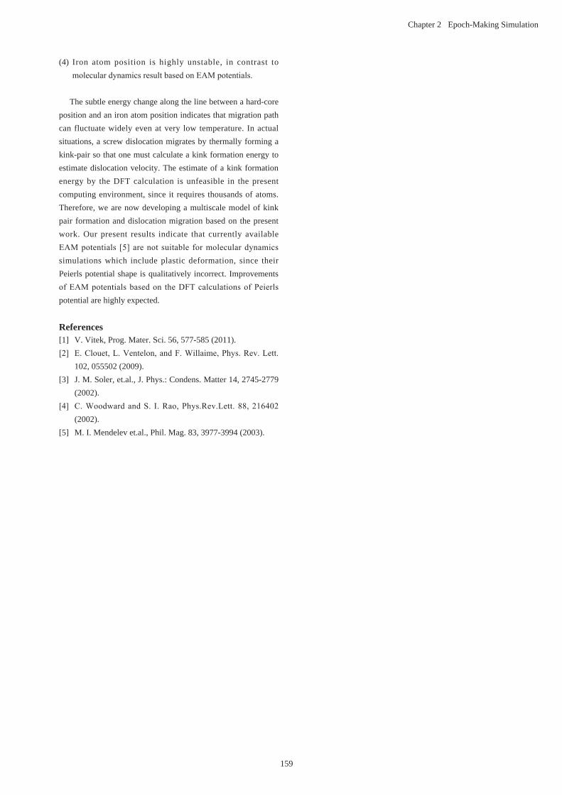
159


(4) Iron atom position is highly unstable, in contrast to molecular dynamics result based on EAM potentials.

The subtle energy change along the line between a hard-core position and an iron atom position indicates that migration path can fluctuate widely even at very low temperature. In actual situations, a screw dislocation migrates by thermally forming a kink-pair so that one must calculate a kink formation energy to estimate dislocation velocity. The estimate of a kink formation energy by the DFT calculation is unfeasible in the present computing environment, since it requires thousands of atoms. Therefore, we are now developing a multiscale model of kink pair formation and dislocation migration based on the present work. Our present results indicate that currently available EAM potentials [5] are not suitable for molecular dynamics simulations which include plastic deformation, since their Peierls potential shape is qualitatively incorrect. Improvements of EAM potentials based on the DFT calculations of Peierls potential are highly expected.

References[1] V. Vitek, Prog. Mater. Sci. 56, 577-585 (2011).[2] E. Clouet, L. Ventelon, and F. Willaime, Phys. Rev. Lett.

102, 055502 (2009).[3] J. M. Soler, et.al., J. Phys.: Condens. Matter 14, 2745-2779

(2002).[4] C. Woodward and S. I. Rao, Phys.Rev.Lett. 88, 216402

(2002).[5] M. I. Mendelev et.al., Phil. Mag. 83, 3977-3994 (2003).

160


第一原理計算による BCC鉄中らせん転位のパイエルスポテンシャルの計算


蕪木　英雄　　日本原子力研究開発機構

著者板倉　充洋 *1，蕪木　英雄 *1，山口　正剛 *1，圓戸　辰郎 *1，樋口　健二 *1，尾方　成信 *2，君塚　　肇 *2

*1 日本原子力研究開発機構

*2 大阪大学

第一原理計算により BCC鉄中の一本のらせん転位のパイエルスポテンシャルを計算した。パイエルス障壁は転位のバガースベクトルの長さあたり 0.04eV であった。また、ハードコアの転位位置の周囲では二次元パイエルスポテンシャルがほぼ平坦になることが分かった。これらの結果は現在使われている分子動力学ポテンシャルの性質とは顕著に異なり、塑性変形を含む分子動力学計算のためには改良されたポテンシャルが必要であることが分かった。

キーワード : 第一原理計算 , らせん転位 , BCC鉄 , パイエルスポテンシャル

161


1. Purpose of the project The purpose of this project is to simulate the three-

dimensional vortices from a circular cylinder in the fluid-flow by using a massively parallel Lattice Gas Method, which is expected to provide excellent computing performance on a large scale vector computer, and to evaluate the applicability of the method by comparing the results with those of experiments or numerical calculations by solving Navier-Stokes equations.

In particular, we try to realize the fluid-flow simulation at high Reynolds numbers by using a new viscosity-control method without increasing the number of nodes of lattice.

2. Plan of three-year researchWe are trying to complete the following three subjects in

three years.(1) Improvement of the calculation-efficiency of massively

parallel bit-wise operation method in the FY 2010.

(2) Confirmation on the simulation results of vortices shedding from a circular cylinder of finite length in the FYs 2010 and 2011.

(3) Simulation of the fluid-flow at high Reynolds numbers by the new viscosity-control method in the FYs 2011 and 2012.

3. Calculation method3.1 Background of the calculation method

According to the previous study[1], it is known that wind or water tunnels can be indifferently used for testing low Mach number flows, provided the Reynolds numbers are identical. Indeed, two fluids with quite different microscopic structures can have the same macroscopic behavior because the form of the macroscopic equations is entirely governed by the microscopic conservation laws and symmetries. Such observations have led to a new simulation strategy for fluid dynamics: fictitious micro-world models obeying discrete cellular automata rules

Development of a Fluid Simulation Approach by Massively Parallel Bit-wise Operations with a New Viscosity Control Method


Hiroshi Matsuoka Research Institute of Electrical Communication, Tohoku University

Authors

Hiroshi Matsuoka*1, Noriko Kikuchi*1*2, Tadashi Watanabe*3, Mitsuo Yokokawa*4, Shin-ichi Mineo*4, Ken-ichi Itakura*5, Yukio Iwaya*1, Yukio Fujinawa*6 and Yoshihiko Orita*7

*1 Research Institute of Electric Communication, Tohoku University

*2 Customer System Company

*3 Japan Atomic Energy Agency


*5 The Earth Simulator Center, Japan Agency for Marine-Earth Science and Technology

*6 Fujinawa Earthquake Research & Development

*7 Japan Marine Science Foundation

The purpose of this project is to simulate the three-dimensional vortices from a circular cylinder in the fluid-flow by using a massively parallel Lattice Gas Method, which is expected to provide excellent computing performance on a large-scale vector computer, and to evaluate the applicability of the method to similar large-scale fluid-simulation problems by comparing the results with those of experiments or numerical calculations by solving Navier-Stokes equations. In particular, we try to realize the fluid-flow simulation at high Reynolds numbers by using a new viscosity-control method that we call "multi-stage collisions of two particles". In case of the method, propagation of particles occurs after several times of collisions of randomly selected two particles at each node. By using the method, we can calculate fluid-flow at somewhat higher Reynolds number without increasing the number of nodes of lattice. Another feature of our method is "massively parallel bit-wise calculations". We obtained the value of 92.8% as the calculation-efficiency by using 576 vector CPUs of Earth Simulator. We regard that the value is a good performance.

Keywords: lattice gas automaton, fluid dynamics, massively parallel computing, vortex from a cylinder, vector computers.

162


have been found, such that two- and three-dimensional fluid dynamics are recovered in the macroscopic limit. The class of cellular automata used for the simulation of fluid dynamics is called "lattice gas models", and many lattice gas models have been proposed.

In our study, we use one-speed models for the simulation of fluid dynamics. The relevant aspects of the models are as follows: there is a regular lattice, the nodes of which are connected to nearest neighbors through links of equal length; all velocity directions are in some sense equivalent and the velocity set is invariant under reversal; at each node there is a cell associated with each possible velocity.

Each node can be occupied by one particle at most; particles are indistinguishable; particles are marched forward in time by

successively applying collision and propagation rules; collisions are purely local, having the same invariances as the velocity set; and collisions conserve only mass and momentum.

3.2 FCHC model for three-dimensional simulationIn order to simulate three-dimensional vortices shedding

from a circular cylinder, we selected a face-centered-hypercubic (FCHC) model among from several one-speed models. The FCHC model is a four-dimensional model introduced by d'Humiéres, Lallemand, and Frisch in 1986[2]. Three dimensional regular lattices do not have enough symmetry to ensure macroscopic isotropy. The detailed FCHC model that we use in this study and the schematic diagram of simulated flow are explained in the following three figures.

Fig. 1 Cells and nodes for simulating the three dimensional vortices shedding from a circular cylinder.

Fig. 2 Propagation rules from node to node.

163


As shown in Fig. 1, the coordinate X is the direction of flow, and the coordinate Z is parallel to the circular cylinder. A position of (X, Y, Z) represents the position of each cell. Every cell contains 32 nodes as depicted in Fig. 1. Each node exists in the four-dimensional space. The fourth coordinate R is represented by the radius of sphere at each three-dimensional position.

As shown in Fig. 2, particles can have 24 kinds of velocities, that is, (ΔX ΔY, ΔZ, ΔR) = (±1, ±1,0,0), (±1,0, ±1,0), ( ±1,0,0, ±1), (0, ±1, ±1,0), (0, ±1,0, ±1) or (0,0, ±1, ±1), and the magnitude of the velocities is equal to √

–2, when the interval between two nearest nodes has a unit length.

Many particles propagate from node to node and make a collision at each node. The rules of propagation and collision are presented in Fig. 2 and Fig. 3, respectively.

The features of our method are "massively parallel bit-wise calculations" and "multi-stage collisions of two particles".

Bit-wise parallel calculations are realized by vector operations on the arrangement representing the state of a cell. The arrangement is given by the form of 4-dimensional integer arrangement bit[D][Z][Y][X] that has 32 elements with the value of "1" or "0". If the k-th bit of the arrangement bit[D][Z][Y][X] equals to "1", this means that a particle moving toward the direction D exists at the k-th node of the cell locating at (X,Y,Z). "1" or "0" means existence or nonexistence of a particle, respectively.

Multi-stage collisions of randomly selected two particles at each node are useful for making a smaller correlation between fluid-velocities of two different cells a little apart from each other. This means that the fluid has smaller viscosity and simulation at higher Reynolds numbers becomes somewhat easier.

Fig. 4 A transient simulation result of the flow past a circular cylinder of infinite lenngth.

Fig. 5 Preliminary simulation of the flow past a circular cylinder of finite length.

Fig. 3 Collision rules at each node.

164


3.3 Results of the study in FY 2010Regarding the improvement of the calculation-efficiency of

"massively parallel bit-wise calculations", we obtained the value of 92.8% by using 576 vector CPUs of Earth Simulator. We regard that the value is a good performance.

As for the three-dimensional simulation, we, at first, numerically simulated the vortices shedding from a circular cylinder of infinite length. Figure 4 shows the results of transient simulation of the fluid-momentum on the plane that Z equals to a certain constant value. General feature of the transient from twin vortices to Karman whirlpools is conceptually equal to those of the experiments by Taneda[3].

T h e n u m b e r o f n o d e s f o r t h e c a l c u l a t i o n i s 3072(X)×768(Y)×768(Z)×4(R) in four dimensional space. We, secondly, tried to simulate the vortices shedding from a circular cylinder of finite length. One of the results is shown in Fig.5. There seems to be indications similar to the calculated result shown by Inoue and Sakuragi[4]. Further study is need in FY 2011.

Acknowledgement

We greatly appreciate JAMSTEC for giving us a chance of using Earth Simulator and very kind support for our study.

References [1] U. Frisch, D. d'Humiéres, B. Hasslacher, P. Lallemand, Y.

Pomeau, and J-P. Rivet, "Lattice Gas Hydrodynamics in Two and Three Dimensions", Complex Systems, 1(1987), pp.649-707.

[2] D. d'Humiéres, P. Lallemand, and U. Frisch, Europhys. Lett., 2 (1986), p.291.

[3] Sadatoshi Taneda, "Gazou kara manabu ryuutairikigaku" (in Japanese), Asakura-shoten, p.45 and p.47.

[4] Osamu Inoue and Akira Sakuragi, "Vortex shedding from a circular cylinder of finite length at low Reynolds numbers", PHYSICS OF FLUIDS, 20(2008), 033601.

165


新粘性制御法による超並列ビット演算流体シミュレーション手法の開発


松岡　　浩　　東北大学　電気通信研究所

著者松岡　　浩 *1，菊池　範子 *1*2，渡辺　　正 *3，横川三津男 *4，峯尾　真一 *4，板倉　憲一 *5，岩谷　幸雄 *1，藤縄　幸雄 *6，折田　義彦 *7

*1 東北大学　電気通信研究所

*2 カストマシステム株式会社

*3 日本原子力研究開発機構



*6 藤縄地震研究所

*7 日本海洋科学振興財団

本プロジェクトの目的は、大規模ベクトル計算機において優れた計算性能を発揮することが期待される格子ガス法超並列計算法を用いて、流体流れの中に置かれた円柱後流に生じる 3次元渦のシミュレーションを行い、その結果を実験やナビエ・ストークス方程式を解く数値計算の結果と比較することによって、同様な大規模流体シミュレーション問題への本手法の適用可能性を評価することにある。特に、“多段 2体粒子衝突”と呼ぶ新しい粘性制御法を用いて、高いレイノルズ数領域における流体流れのシミュレーションの実現をめざす。この手法では、各ノードにおいて、ランダムに選択された 2粒子が数回衝突を起こしたあとに、粒子の並進移動を行う。本手法を用いると、格子点の数を増やすことなく、ある程度高いレイノルズ数領域の流体流れを計算することができる。我々が提案する手法のもうひとつの特徴は、“超並列ビット計算”である。地球シミュレータの 576個のベクトル CPUを用いて、並列化効率 92.8%という値を得た。

キーワード : 格子ガスオートマトン , 流体力学 , 円柱後流 , 超並列計算 , 円柱後流渦 , ベクトル計算機

167


1. IntroductionThe RSA cryptography code is the most important key

technology for using the Internet safely; however, the currently used 1,024-bit RSA code will no longer be safe to use in near future. The RSA cryptography code is based on the difficulty of the factorization of long-digit composite numbers, and the decryption time of 1,024-bit RSA code is several tens of years even if the fastest supercomputer is used. For an RSA code with a particular number of bits to be safe, its decryption time using the fastest algorithm on the fastest supercomputer must be more than 10 years.

The present world record for RSA decryption, involving RSA-768 (768 bits, 232 digits) was performed by a team consisting of NTT and four foreign organizations in January 2010. It took 1,677 CPU-years to decrypt. This means that if one core of a PC CPU (AMD64, 2.2 GHz) is used, then it will take 1,677 years to decrypt. All reported world records for RSA decryption were carried out using PC clusters; however, there has been no report regarding this challenge for vector supercomputers. Therefore, a test using a vector supercomputer is necessary for the precise evaluation/discussion of the safety of 1,024-bit RSA cryptography codes.

This project intends to obtain basic information for processing RSA decryption on the Earth Simulator 2 (ES2), which is a vector supercomputer. The decryption processing consists of three parts: the first step is "sieve processing", the second step is the processing of 0-1 matrices, and the third step is the computation of algebraic square roots. For RSA-768, the

first step, sieve processing, was about 90% of the computation time to decrypt. In 2010, the first year of our project, the author tuned the sieve processing part of the decryption code on the ES2.

2. RSA codeThe common key cryptosystem and the public key

cryptosystem are basic cryptosystems. The common key cryptosystem has only one key. It is simple and fast to process, but sending the key via the internet represents a problem. The public key cryptosystem has two different keys, one each for encryption and decoding. The key for encryption is open to the public, and the key for decoding can be kept secure because it is not necessary to send this key. A set of keys for the public key cryptosystem is based on the RSA code, which was developed by R. L. Rivest, A. Shamir, and L. M. Adleman in 1978. The RSA code uses two long-digit prime numbers P and Q, and a prime number e to compute n = P*Q, F = (P - 1)*(Q - 1), and D = e-1 (mod F). Numbers n and e are used as the keys for encryption, and the number D is used for the key for decoding. The safeness of this system is based on the result that, for a given long-digit number n, the factorization algorithm of n to P and Q has high computational complexity and consumes enormous computation time.

3. Sieve methodThe sieve method is a factorization method for composite

numbers N which obtains a relationship a2 - b2 = 0 (mod N) for

RSA Decryption using Earth Simulator


Hidehiko Hasegawa Graduate School of Library, Information and Media Studies, University of Tsukuba

Author

Yasunori Ushiro Department of Mathematics, School of Education, Waseda University

RSA cryptography code is the key technology for safe Internet use and currently a 1,024-bit RSA code is used. To guarantee the safety of RSA code, a decryption time of more than 10 years, even using the fastest supercomputer, is necessary. The present world record for RSA decryption, involving RSA-768 (768 bits), took 1,677 CPU-years to decrypt. So with 1,024-bit RSA code, it is expected to take in the range of 10 to 100 years. All world records for RSA decryption, including that for RSA-768, were carried out by PC clusters. Decryption has never been attempted using a vector supercomputer.

To confirm the decryption time on a vector supercomputer, the author is trying to tune the RSA decryption code for the Earth Simulator 2 (ES2). The RSA cryptography code is based on the difficulty of the factorization of long-digit composite numbers, and the decryption code consists of three parts: "sieve processing", processing of 0-1 matrices, and computation of algebraic square roots. Sieve processing was chosen as the first target for tuning because of its computation time. Sieve processing is tuned, and its performance on one node of the ES2 is approximately 800 times faster than that on a PC (Intel Core 2, 2.3 GHz). This processing is about 99.9% vectorized with few floating point number operations, and it is suitable for the vector supercomputer.

Keywords: RSA code, Sieve processing, Vector processing, non-floating point number operations, GNFS, Decryption

168


some a, b. Because natural numbers a and b are constructed by products of prime numbers provided by the sieve, the exponent of each prime number must be an even number.

For a composite number N, we assume X is the nearest integer to N1/2 and calculate (X + k)2 - N = Ak, k = 0, 1, 2, …. Then, we collect Ak that can be factorized using only prime numbers in factor base P. We can factorize N into a product of prime numbers with a combination of Ak whose exponent part is even. This provides the squared form a2 - b2 = 0 (mod N). Multiple polynomial quadratic sieve (MPQS) uses many types of quadratic equations.

Again for a composite number N, we find a polynomial f(x) and a number M such that f(M) = 0 (mod N). Let θ be an algebraic root of the equation f(x) = 0. We factor a + bM using prime numbers, and factor a + bθ using algebraic elements of primes and the unit. The difference in these factorizations is used for the decryption. For example, let N = 1333, f(x) = x3 + 2, f(M) = N, and M = 11; then 2 + M = 13 and 2 + θ = θ(1 - θ)(1 + θ). Then, 11∙(-10)∙12=13 (mod 1333) is established. However, we cannot find algebraic elements of primes for any f(x). Therefore, we use a prime ideal in the general number field sieve (GNFS). We define the polynomial norm as N(θ) = |f(-a/b)| for ideal a + bθ, and factorize N(θ) with the prime numbers in the ideal base.

It is said that MPQS is faster for the factorization of fewer than 100 digits, and GNFS is faster for the factorization of more than 100 digits.

For RSA-768, the factorization was carried out using a linear equation and a sixth-order polynomial in the GNFS. The computational complexity of RSA-768 in PC-years of an AMD64 (2.2 GHz) is shown in Table 1.

4. Sieve programming on the ES2The sieve processing is the most time-consuming part of both

MPQS and GNFS. The kernel is as follows:

do k=1,N N is the number of elements in the basedo i = Start(k), LP, Prime(k) Start(k): start, Prime(k): increment

V(i) = V(i) + Log(P(i))end do

end dodo i = 1,LP < Collection of sieved data >

if(V(i) .le. PS(i)) then condition of collectionns = ns + 1 ns is the number of collected dataSieve(ns) = LLP + i store the position of each collected data

end ifend doUpdate Start(1) through Start(N) for the next sieve

Here, the LP is the length for the sieve, Prime(k) is the prime number in the base, and Start(k) is the starting number that it is factorized with prime numbers in the base. For speeding up computation on a PC, LP*4 bytes has to be completely allocated in the cache (1 MB). On the other hand, for the factorization of a 200-digit number, N is at least tens of millions and the value of LP reaches hundreds of millions. To reduce computational complexity, a larger N is necessary but to speed up computation on a PC, a smaller N is necessary. Thus, processing large prime numbers on a PC is very inconvenient.

On the vector supercomputer ES2, a larger LP value can be used and its length becomes the vector length of the ES2. However, for the collection of sieve data part, performance was not good, as expected, because there are almost no calculations. This part was vectorized using a data compaction operation; however, the hit ratio can be once hundreds of millions. The code was modified as follows: first, the existence of adopted data in tens of thousands of intervals was checked, and then the collecting procedure was applied only if the interval had adopted data. Using this modification, the whole sieve process became approximately 3 times faster than the original version on the ES2.

In the sieve processing, the sieve whose loop length is LP, is performed for each prime number. As the sieve processing needs less communication in parallel computing environments, it is easy to parallelize by using MPI.

Table1 Computational complexity of RSA-768 (232 digits).

PC-years Ratio (%)Exploration of polynomial 20 1

Sieve processing 1500 900-1 matrices processing 155 9Algebraic square root 1 0

Others 1 0Total 1677 100

Table 2 Specification of PC and vector computer.

PC Vector computer

ComputerDell Vostro 200

Intel Core 2 2.3 GHz, 2GB

Earth Simulator (ES2)3.2 GHz

1 node: 819 Gflops,128 GB

Measurement 1 core Measured by CPU time

1 node (8 CPU)Measured by use time

Software Windows Vista, g77 -O3 Option

NEC SUPER-UXAuto vector FORTRAN + MPI

169


5. Comparison of the sieve processingThe specifications of the PC and the vector computer are

listed in Table 2.The author measured the sieve processing for 45- and

60-digit numbers. This is equivalent to the sieve processing of 90 digits and 120 digits in MPQS, and the sieve processing of approximately 130 digits and 170 digits in GNFS. The author used N prime numbers in the base, in ascending order. The computation time greatly depends on the number of elements in the base. The size of LP is 512K on a PC, and 1G on the ES2. Figure 1 shows the result for 45 digits, and Fig. 2 shows that for 60 digits. The computation time on a PC is divided by 200 in both figures.

In both Figs. 1 and 2, the fast range in terms of the number of elements in the base is wider and the numbers are larger on the ES2 than those for the PC. This means that the better performance has been attained on the ES2 for most cases.

It is necessary to include more primes in the base as the number of digits of the factorized number increases. Figure 3 shows the best speed-up ratio of the ES2 over a PC by the number of primes in the base. The left dashed rectangular region is an estimation of 150 digits in MPQS. The speed-up ratio of the ES2 over a PC increases if more primes in the base are used. The ES2 is approximately 600 times faster than the PC for 150 digits of MPQS and is estimated to be approximately 800 times

faster for the equivalent RSA decryption size.

6. SummaryThe author tuned the most time-consuming part, sieve

processing, in the RSA decryption processing. The following basic information was obtained:1) This processing is about 99.9% vectorized with few floating

point number operations, and it is suitable for a vector supercomputer.

2) The performance of the sieve processing on one node of the ES2 is approximately from 200 to 800 times faster than that of a PC (Intel Core 2, 2.3 GHz).

3) The performance ratio for a realistically scaled RSA decryption is expected to be approximately 800.For the second year of this study, the author will modify the

sieve processing in the GNFS, measure its computation time for from 100 digits to 200 digits, progressively, and then estimate the computation time of GNFS for more than 200 digits. The author will also tune the 0-1 matrices processing.

AcknowledgementThe author expresses his thanks to Dr. Yoshinari Fukui

and Dr. Toshiyuki Asano of JAMSTEC, who provided vital suggestions for greatly speeding up computation on the ES2.

Fig. 1 Sieve processing of 45 digits.

Fig. 2 Sieve processing of 60 digits.

Fig. 3 Speed-up ratio of the ES2 over a PC.

170


References [1] Richard A. Mollin, "RSA and PUBLIC-KEY CRYPTOG-

RAPHY", Chapman and Hall/CRC, 2002.[2] Yuji Kida, "Prime factoring by General Number Field

Sieve", 2003. http://www.rkmath.rikkyo.ac.jp/~kida/nfs_intro.pdf (in

Japanese)[3] Jun'ichi Yamazaki and Souta Kamaike, "The 2010 problem

of the Cryptography", ASCII technologies, 75-93, Sept. 2010. (in Japanese)

[4] Neal Koblitz, translated by Kouichi Sakurai, "A Course in Number Theory and Cryptography ", Springer, 1997. (in Japanese)

[5] Kazumaro Aoki, "Advances in Integer Factoring Technique: The Way to Factor RSA-768", IPSJ Magazine, 51(8), 1030-1038, Aug. 2010. (in Japanese)

[6] Yasunori Ushiro, "A high speed sieve computation for the RSA decryption by the vector computer", RIMS kokyuroku, No.1733, 101-117, March 2011. (in Japanese)

171


地球シミュレータを用いた RSA暗号解読処理


長谷川秀彦　　筑波大学大学院　図書館情報メディア研究科

著者後　　保範　　早稲田大学　教育学部　数学科

ES2 において RSA 暗号解読の大半の時間を占める「ふるい処理」の高速化を行い、ES2 1 ノードで PC １コアの約 800倍の性能を達成した。

RSA 暗号はインターネットを安全に使ううえで欠かせない技術である。しかし、現在使用している 1024 ビットのRSA 暗号が安全性の問題で近いうちに使えなくなるという「2010 年問題」が懸念されている。RSA 暗号には桁数の多い合成数の因数分解の困難性が利用されており、1024 ビット RSA 暗号の安全性はスーパーコンピュータを数年使用しても解読されないという仮定のもとで成り立っている。いっぽう、2010 年 1 月に NTT 他 4 カ国の共同で実施された RSA暗号解読の世界記録（RSA-768）をはじめ、今までのすべての世界記録は PC クラスタで達成されており、ベクトル方式のスーパーコンピュータによる RSA 暗号の解読実験は全く報告されていない。そこで、代表的なベクトル方式のスーパーコンピュータである地球シミュレータ（ES2）において RSA 暗号の解読実験を行う。

一般的な RSA 暗号解読は、ふるい処理、0-1 行列処理、代数的平方根の計算の 3 段階からなり、これまでの RSA 暗号解読プログラムはすべて PC 用となっている。本年度は、RSA 暗号解読の大半の処理時間を占める「ふるい処理」とES2 の相性を評価した。PC クラスタにおける RSA-768 ではふるい処理が全体の約 90% を占めている。試行錯誤の結果、ES2 で効率よくふるい処理を行うにはふるい結果のデータを集める処理の対策が重要であることが判明した。これらはPC における対策とは大幅に異なっているが、ES2 とふるい処理の相性は良いことが分かった。数値実験では、800 bit 相当のふるい処理において ES2 の 1 ノードで 2.3GHz の PC １コアの 800 倍程度の性能を達成した。このとき、浮動小数演算はほとんどないがベクトル化率は 99.9% で、この結果を単純に外挿すると ES2 32 ノード、2TB（64GB/ ノード）を用いた RSA-768 のふるい処理に要する時間は 21 日となる。

本年度は、0-1 行列処理の部分を ES2 向けに書き換えること、ふるい処理と 0-1 行列処理を合わせて 1024 bit の RSA暗号の解読に要する時間を推定するための基礎的データの取得を行う予定である。

キーワード : RSA暗号 , ふるい処理 , ベクトル処理 , 整数演算 , GNFS

謝辞地球シミュレータ（ES2）における高速化について、貴重なご意見を頂いた海洋研究開発機構地球シミュレータセンター

の福井義成氏及び浅野俊幸氏に謹んで感謝の意を表する。

参考文献[1] Richard A. Mollin, "RSA and PUBLIC-KEY CRYPTOGRAPHY", Chapman and Hall/CRC , 2002 年[2] 木田　祐司 , " 数体ふるい法による素因数分解 ", 2003 年 http://www.rkmath.rikkyo.ac.jp/~kida/nfs_intro.pdf[3] 山崎　潤一 , 釜池聡太 , " 暗号の 2010 年問題 ", ASC Ⅱ Technologies, 75-93,2010 年 9 月[4] N. コブリッツ , 桜井幸一訳 ," 数論アルゴリズムと楕円暗号理論入門 ", シュプリンガー・フェアラーク東京 , 1997 年[5] 青木和磨呂 , " 素因数分解技術の進展： RSA-768 の分解達成への道のり ", 情報処理 , 51(8), 1030-1038, 2010 年 8 月[6] 後　　保範 , " ベクトル計算機による RSA 暗号ふるいの高速化 ", 京大数理研講究録 , No. 1733, 101-117, 2011 年 3 月

173


1. IntroductionA study[1] for establishing a simulation analysis method

using the explicit finite element impact analysis code LS-DYNA[2] was conducted on the shaking table test of the full-scale six-story reinforced concrete (RC) building, which can analyze the behavior of RC buildings under strong seismic loading close to the near collapse of the building structure.

An analysis of the seismic response was conducted for a sophisticated model of the main wall-frame of the six-story RC building in a damage-free fresh condition, based on the experimental data of full-scale building structure tested

on the shaking table at the Hyogo Earthquake Engineering Research Center (E-Defense) with input seismic waves (input acceleration factor of 100%) equivalent to those recorded during the 1995 Hanshin-Awaji earthquake. Displacement response of the analytical result was smaller than that recorded in the experiment. The authors considered that one of the causes that affected such a difference was the cumulative damage of the building under the test loads, which occurred by gradually increased shaking intensity (prior shaking) before application of the actually measured waves (100%). Accordingly, analyses that consider the cumulative damage caused by such prior shaking

Development of Sophisticated Simulation Analysis Method of Actual Reinforced Concrete Building by Shaking Table Test–I


Yoshiyuki Kasai Department of Urban Environment and Information Sciences, Graduate School,Maebashi Institute of Technology

Authors

Yoshiyuki Kasai

Haruji TsubotaYoshikazu Kanai

Shigefumi TakedaKazukuni NiwaYoshio Manabe

Department of Urban Environment and Information Sciences, Graduate School, Maebashi

Institute of Technology.

Department of Architecture, Graduate School, Maebashi Institute of Technology.

Department of Urban Environment and Information Sciences, Graduate School, Maebashi

Institute of Technology.

Department of Architecture, Graduate School, Maebashi Institute of Technology.

Terrabyte Co, Ltd.

Terrabyte Co, Ltd.

A study[1] for establishing a sophisticated simulation analysis method utilizing an explicit finite element impact analysis method was conducted for the model comprising about 2.08 million elements of the main wall-frame of the actual scale six-story reinforced concrete building (total mass about 1,000 tons), which was tested on the shaking table with the input of seismic waves equivalent to those recorded in the 1995 Hanshin-Awaji earthquake. The results of the analysis show that the displacement response subjected to the actually measured waves (input acceleration factor of 100%) corresponding to a seismic intensity scale of 6 upper is smaller than that measured in the experiment. In the experiment, the intensity of the input waves increased in steps to 100%. The authors considered that cumulative damage to the structure caused by shaking before 100% intensity input waves is one of causes that affected such a difference and, therefore, conducted an analysis that considered the effects of the cumulative damage. The displacement response from such an analysis corresponded more closely to the results of the experiment. Analyses were also conducted for a fresh model free of cumulative damage by applying the input acceleration factor of 120%, 150%, and 200%, respectively, and the results were compared with the results of the experiment. The results of the analyses with an input acceleration factor between 120% and 150% corresponded to the results of the experiment. The analyses also indicated that the building would collapse when 200% input waves were applied. The authors intend to increase the number of analyses for various cases and then compare and verify such analyses with the results of experiments so that numerical shaking experiments can be conducted with this simulation analysis program for assessment of seismic safety under severe seismic conditions.

Keywords: Seismic response, Shaking table test, RC frame, Earth simulator, FEM simulation

174


were conducted, and the results were in comparatively good agreement with the experimental results.

2. Outline of shaking table test of an full-scale six-story RC buildingThe experiment that was analyzed was the shaking table

test of the full-scale six-story RC building conducted in E-Defense. The data for the test conditions and the building used for the analysis were taken from the published report[3]. The structure of the building used for the analysis was the six-story, three-dimensional wall-frame consisting of two spans in the x-direction and three spans in the y-direction, and each span had a dimension of 5,000 mm, a floor-to-floor height of 2,500 mm, and overall building height of 15,000 mm. The test was conducted with seismic waves equivalent to those recorded at the Kobe Marine Observatory of the Japan Meteorological Agency during the 1995 Kobe-Awaji earthquake (corresponding to the seismic intensity of 6 upper) increasing the input acceleration factor in steps of 5%, 10%, 25%, 50%, and 100%, respectively, and finally 60%. Shaking was applied in three directions horizontally, the x- and y-directions and in the vertical direction, with the original seismic waves rotated 45 degrees,

the N45W direction in the y-direction of the building under test, and the N45E direction in the x-direction. Based on such an application, the intention was that the ultimate fracture of the building would take place in the y-direction.

3. Summary of analysis3.1 Analytical model

Figures 1 through 4 show the outline of the model used in the FEM analysis. In the model, concrete was represented as solid elements, and reinforcing bars were represented as beam elements as they were in the actual state; the concrete and reinforcing bar elements have common nodes assuming full adhesion between them. The foundation of the building was not represented in the model but represented as rigid shell elements where the bases of the columns were anchored. Input of the seismic waves was applied at the rigid shell elements in the analysis of the seismic response. The size of the analysis model was about 1.48 million elements for concrete, about 0.57 million elements for reinforcing bar, and about 30,000 elements for the rigid shell for total of about 2.08 million elements, and the total number of nodes was about 1.79 million. The material model installed in LS-DYNA[4] was used. Figure 5 shows the stress (σ)

Fig. 1 View of the entire analytical model (Color-coded for input data layer recognition category).

Fig. 2 Reinforcing bar model of the main frame.

Fig. 3 Enlarged view of the reinforcing bar model of the main frame.

Fig. 4 Reinforcing bar model of the earthquake resistant wall.

175


and strain (ɛ) relationship of the material model used. For the concrete element, the material model[5,6] was used

with characteristics of Ottosen's fracture criterion[7], smeared cracks, etc. in consideration of strain rate effect stress relaxation in tension was dependent on the fracture energy and the crack width. For the reinforcing bar element, an isotropic elastic-plastic model in consideration of kinetic hardening was used, which is a bi-linear type where the plastic hardening coefficient after the yield is 1/100 of the elastic modulus.

Fig. 5 Material model.

Concrete model Reinforcing bar model

3.2 Conditions of seismic response analysisIn this analysis, an explicit dynamic finite element method

was used. Consideration was given wherein the application of the load due to gravitational acceleration was increased gradually from 0 m/s2 to 9.8 m/s2 during the 0 to 0.6 seconds before the application of the seismic waves, which started at 0.6 seconds. Because of the large volume of data in the analysis of the six-story RC building, it took about 2 hours using 16 nodes (128 CPUs) of the Earth Simulator for calculation of the initial 1.0 seconds. After 1.0 seconds, it took about 3 hours for calculation of the next 1.0-second possibly due to the increased computing task load in treating the plastic region and fracture of the materials. Because use of the Earth Simulator for one operation is restricted to 12 hours, analysis for about 4 seconds was possible with 16 nodes (128 CPUs) used in one operation (12 hours) in the case of the analysis of the six-story RC building. Restarting the analysis was made up to 4.6 seconds in the case of no prior shaking and up to 13.6 seconds in the case of application of prior shaking, which was the remaining computing task. Damping characteristics in proportion to the mass with damping coefficient of 3% was considered. Central difference time integration in the explicit finite element method was used, and the time interval of about 3.8 microseconds (3.8×10-6s) with the data output interval of 1.0 milliseconds (1.0×10-3s) was used.

4. Results of seismic response analysisFigure 6 shows the results of the analysis of the time-history

waveform of the story drift of the first floor in the y-direction with the input acceleration and the experimental results[1]. While the results of the analysis with seismic waves with 100% and 120% input acceleration factors are smaller than the results

of the experiment, the result of the analysis with the 150% input acceleration factor is larger than the results of the experiment, which mean that for seismic waves input into the fresh model that does not take cumulative damage into consideration, analysis with the input acceleration factor between 120% and 150% would correspond to the results of the experiment. When the results of the analysis for the fresh model (Case in Fig. 6) are compared with the results from the model taking cumulative damages into consideration (Case ) with input acceleration factor of 100%, the story drift for Case is considerably greater than that of Case and is close to the story drift measured in the experiment. By the way, cumulative damages occurred in the prior shaking were reproduced by the response due to seismic wave with 100% assumed to be equivalent to the total input effect due to 5%, 10%, 25%, and 50%, before the actually measured wave 100% and therefore Case is subjected to 100%-100% inputs.

The stress conditions of the short columns with the spandrel walls and the foot of the earthquake resistant wall where damage occurred in the experiment was severe, the deformation condition of the concrete skeleton, and the deformation condition of the reinforcing bar are shown in Fig. 7 in the magnified view of the deformation. Figures 7 (a), (b), and (d) through (f) are contour maps showing von Mises equivalent stress, where the stress increases from the cold colored area to the warm colored area. In Fig. 7 (c), the main reinforcing bar of the short columns are resisting the seismic loads and swelling out a little under the constraints of the shear reinforcing bar. As shown in these diagrams, this analysis method allows flexible indication of conditions in detail of the building structure, such as the conditions of the reinforcements, stress conditions at any section of the structural elements, etc.

5 ConclusionThe time history seismic response analysis of the

sophisticated FEM analysis model precisely representing concrete and reinforcing bar of the full-scale six-story RC building using the explicit finite element impact analysis method was conducted. The results of the simulation were consistent with the results of the experiment. The analysis method employed provides excellent features where the dynamic characteristics of the structure are automatically created by the material characteristics of the concrete and reinforcing bar, and by the arrangements, the dimensions, etc., of each structural element. The evaluation of the elastic-plastic characteristics up to large deformation caused by large input acceleration is possible, and the conditions for damage or fracture can be visually presented as the computer animation. Because of the analysis method using explicit algorithms, verification of computational accuracy and analysis results are required, and the method can possibly be used for analysis of the large-scale model and large input acceleration. The authors consider the

176


Fig. 6 Story drift time history.

177


collection of analysis data for increasing the number of examples and verification of such analyses with the results of experiments so that shaking tests can be conducted in a simulation analysis program. When this is possible, the evaluation of shaking under extremely large input acceleration, which is impossible in a shaking table test, will become possible, and evaluation of

seismic safety under severe seismic conditions as in the 2011 Great East Japan earthquake will become possible.

Fig. 7 FEM simulation analytical result (displacement is enlarged by 10 times).

(a) Mises stress contour at X1 frame

(b) Mises stress contour at X1 frame (enlargement)

(c) Displacement at X1 frame reinforcement bar

(e) Mises stress contour at X2 frame (enlargement)

(f) Mises stress contour at X2 frame (enlargement)

(d) Mises stress contour at X2 frame

178


References[1] Shigefumi Takeda, Yoshikazu Kanai, Yoshio Manabe,

Kazukuni Niwa, Yu Narita, Haruji Tsubota, and Yoshiyuki Kasai, "Application of Impact Analysis Code based on the Explicit Time Integration to the Shaking Table Tests of Full-Scale Six Story RC Building, Part 2 ", Bulletin Maebashi Institute of Technology, No.14, pp.17-24, March 2011, (in Japanese ).

[2] LS-DYNA (general purpose transient dynamic finite element program), Livermore Software Technology Corporation (LSTC).

[3] Y. Kim, T . Kabeyasawa, T . Matsumor i , and T . Kabeyasawa, "Analytical Studies on A 6-Story Full-Scale Reinforced Concrete Wall-Frame Structure to Collapse ", The 14th World Conference on Earthquake Engineering, October 12-17, 2008, Beijing, China.

[4] Livermore Software Technology Corporation (LSTC), "LS-DYNA KEYWORD USER'S MANUAL VOLUME I, II".

[5] B.J. Broadhouse, "The Winfrith Concrete Model in LS-DYNA3D", Report: SPD/D(95)363, Structural Performance Department, AEA Technology, Winfrith Technology Centre, U.K. (1995).

[6] B.J. Broadhouse and A.J. Neilson, "Modelling Reinforced Concrete Structures in DYNA3D", Safety and Engineering Division, United Kingdom Atomic Energy Authority, Winfrith, AEEW-M 2465, 1987.

[7] N.S. Ottosen, "Failure and Elasticity of Concrete", RISO-M1801, July 1975.

179


実大鉄筋コンクリート造建物の振動台実験の精密・詳細シミュレーション解析システムの開発　その 1


河西　良幸　　前橋工科大学　大学院工学研究科環境・情報工学専攻

著者河西　良幸　　前橋工科大学大学院工学研究科環境・情報工学専攻

坪田　張二　　前橋工科大学大学院工学研究科建築学専攻

金井　喜一　　前橋工科大学大学院工学研究科環境・情報工学専攻

武田　慈史　　前橋工科大学大学院工学研究科建築学専攻

丹羽　一邦　　株式会社テラバイト

真鍋　慶生　　株式会社テラバイト

実大鉄筋コンクリ－ト造 6 階建物（総質量約 1000t）の阪神淡路大震災での記録地震波を入力とした振動台実験での建物損傷状況の結果を例に、架構各部材をあるがままに精密・詳細な有限要素モデル化（約 208 万要素）し、陽解法の衝撃解析プログラムを適用して精密・詳細なシミュレ－ション解析システムの構築を試みた。震度 6 強相当の実測波形

（100% 入力）による変位応答は実験に比べて小さい結果となった。実験では地震波の入力加速度倍率を順次増大させて与え、その後 100% の入力を行っている。この事前の加震による累積損傷が解析による変位応答が小さい要因のひとつと考え、累積損傷の影響を考慮した解析を行った。その結果、変位応答は比較的良く一致する結果となった。また、累積損傷の無いフレッシュな試験体に地震波の入力加速度倍率を、120%、150%、200% と変化させた解析も行い実験結果と比較した。振幅倍率 120% と 150% の中間程度の入力が実験結果と対応する結果となった。また、建物が倒壊するのは 200% の大きな入力の場合であることも分かった。

採用した解析法は、コンクリートと鉄筋の材料的特性を与え、各部材要素の配置、寸法等によって自ずと力学的な特性が取り込まれ、大入力に対する鉄筋コンクリ－ト建物の大変形までの弾塑性特性が評価でき、更に、損傷や破壊がコンピュータアニメーションとして表現できるという優れた面を持つ解析法である。陽解法というアルゴリズムに基づく方法によるために、計算精度や解析結果の検証という過程が必要であるが、大規模モデル、大入力を扱い得るので、今後更に、解析事例の蓄積、実験結果との比較検証を進め、数値振動実験をシミュレ－ション解析システム上で行えるようにしたい。これにより、振動台実験では不可能な大入力加振の場合を評価し得ることができ、東日本大震災のような従来想定できなかったような過大な地震条件での耐震安全性の評価が可能になる。

キーワード : 地震応答 , 振動台実験 , 鉄筋コンクリート骨組 , 地球シミュレータ , FEMシミュレ－ション

181


1. IntroductionDroplet splashes have been investigated for more than a

century (Worthington 1908). Although droplet splashing is a historical and common research topic, it has not fully been understood. This is because droplet splashing is quite complex and appears as a result of complex interactions among all the physical effects such as the inertia, viscosity, surface tension, gravity, contact angle and roughness. Droplet impacts onto dry surfaces as well as splashes play important roles in many industrial applications such as internal combustion engines (fuel droplets), inkjet printing and spray cooling. Many others have been indicated for example in a review article (Yarin 2005). We aim to study the fundamental of droplet splashing using numerical simulations and to contribute to a wide range of industrial applications through the fundamental study and numerical simulations.

2. Numerical methodWe employ an approach using a regular Cartesian grid

and use the coupled level set and volume-of-fluid (CLSVOF) formulation (Sussman & Puckett 2000), which uses both the level set method (Other & Sethian 1988) and the VOF method (Hirt & Nichols 1981). In this formulation, the VOF method deals with interface motion and the level set method is used for surface tension and wettability computations. In this paper, the tangent of hyperbola for interface capturing/weighed line interface calculation (THINC/WLIC) method (Xiao et al., 2005, Yokoi 2007) is used instead of the VOF/piecewise linear interface calculation (PLIC) method. Although the THINC/WLIC method is a type of VOF method and satisfies volume

conservation, it is easy to implement and the numerical results from the THINC/WLIC method appear to be similar to the results from the VOF/PLIC method. For the flow calculation, we employ a finite volume framework. The constrained interpolation profile-conservative semi-Lagrangian (CIP-CSL) method (Yabe et al., 2001) is used as the conservation equation solver. Although finite volume methods usually deal with only the cell average as the variable, the CIP-CSL method uses both the cell average and the boundary value as variables. By using both values (moments), a parabolic interpolation function is constructed in a cell, and the boundary value and the cell average are updated based on the parabolic function. For multidimensional cases, dimensional splitting is used (Xiao et al., 2002). The volume/surface integrated average based multi moment method (VSIAM3) (Xiao et al., 2005, 2006) is a fluid solver which can be combined with the CIP-CSL methods. For the surface tension force, we use the CSF (continuum surface model) model (Brackbill 1992). For more detail see (Yokoi 2008, Yokoi et al., 2009).

3. Governing equationWe use a finite volume formulation so that we use the

following governing equation of an integral form:∫Γ u·ncdS = 0 (1)д ∫ΩudV + ∫Γ u(u·nc)dS = – 1 ∫Γ pncdS + 1 ∫Γ (2µD)·ncdS +

1 Fsf + gдt ρ ρ ρ

(2)

Where u is the velocity, nc the outgoing normal vector for the control volume Ω with its interface denoted by Γ, ρ the density, µ the viscosity coefficient, D ≡ 0.5(

Δ

u + (

Δ

u)T), Fsf surface

Numerical Simulations of Droplet Splashing


Feng Xiao Interdisciplinary Graduate School of Science and Engineering, Tokyo Institute of Technology

Authors

Kensuke YokoiFeng Xiao

School of Engineering, Cardiff University

Interdisciplinary Graduate School of Science and Engineering, Tokyo Institute of Technology

We perfumed numerical simulations of droplet splashing (single droplet impacting, multiple droplets impacting, and droplet-droplet collisions). The numerical framework is based on a CLSVOF (coupled level set and volume-of-fluid) method, the THINC/WLIC (tangent of hyperbola for interface capturing/weighed line interface calculation) method, the CIP-CSL (constrained interpolation profile-conservative semi-Lagrangian) method, VSIAM3 (volume/surface integrated average based multi moment method) and CSF (continuum surface force) model. Our numerical framework can reproduce a prompt splash with satellite droplets and spikes at least qualitatively. The framework can also qualitatively reproduce droplet coalescence and separation of Weber number 30. We also conducted numerical simulations of five droplets splashing and collision of two droplets of Weber number 1000.

Keywords: droplet, splash, coalescence, CLSVOF, THINC/WLIC, CIP-CSL, VSIAM3

182


tension force, g the gravity acceleration. Equations (1) and (2) are solved by a multi moment method based on the CIP-CSL method and VSIAM3.

4. Numerical results4.1 Droplet splashing on dry surfaces

We conducted three dimensional numerical simulations of droplet splashing on super hydrophobic substrates. As a validation, we compare a numerical result with the experiment

Fig. 3 Five droplets impacting onto a dry surface.

Fig. 1 A comparison between a numerical result of droplet splashing and the experiment (Tsai et al., 2009).

Fig. 2 A numerical resul t of s ingle drople t splashing.

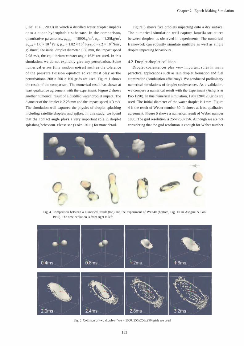
183


(Tsai et al., 2009) in which a distilled water droplet impacts onto a super hydrophobic substrate. In the comparison, quantitative parameters, ρliquid = 1000kg/m3, ρair = 1.25kg/m3, µliquid = 1.0 × 10-3 Pa·s, µair = 1.82 × 10-5 Pa·s, σ =7.2 × 10-2N/m , g9.8m/s2, the initial droplet diameter 1.86 mm, the impact speed 2.98 m/s, the equilibrium contact angle 163° are used. In this simulation, we do not explicitly give any perturbation. Some numerical errors (tiny random noises) such as the tolerance of the pressure Poisson equation solver must play as the perturbations. 200 × 200 × 100 grids are used. Figure 1 shows the result of the comparison. The numerical result has shown at least qualitative agreement with the experiment. Figure 2 shows another numerical result of a distilled water droplet impact. The diameter of the droplet is 2.28 mm and the impact speed is 3 m/s. The simulation well captured the physics of droplet splashing including satellite droplets and spikes. In this study, we found that the contact angle plays a very important role in droplet splashing behaviour. Please see (Yokoi 2011) for more detail.

Figure 3 shows five droplets impacting onto a dry surface. The numerical simulation well capture lamella structures between droplets as observed in experiments. The numerical framework can robustly simulate multiple as well as single droplet impacting behaviours.

4.2 Droplet-droplet collisionDroplet coalescences play very important roles in many

paractical applications such as rain droplet formation and fuel atomization (combustion efficiency). We conducted preliminary numerical simulations of droplet coalescences. As a validation, we compare a numerical result with the experiment (Ashgriz & Poo 1990). In this numerical simulation, 128×128×128 grids are used. The initial diameter of the water droplet is 1mm. Figure 4 is the result of Weber number 30. It shows at least qualitative agreement. Figure 5 shows a numerical result of Weber number 1000. The grid resolution is 256×256×256. Although we are not considering that the grid resolution is enough for Weber number

Fig. 5 Collision of two droplets. We = 1000. 256x256x256 grids are used.

Fig. 4 Comparison between a numerical result (top) and the experiment of We=40 (bottom, Fig. 10 in Ashgriz & Poo 1990). The time evolution is from right to left.

184


1000, if the numerical resolution is greatly increased on high-end super computers such as ES2, the droplet behaviour would be quantitatively reproduced.

References[1] A. M. Worthington, A study of splashes, Longmans,

Green, and Co., (1908).[2] A. L. Yarin, Annu. Rev. Fluid Mech., 38, 159 (2005).[3] M. Sussman and E. G. Puckett, "A coupled level set

and volume-of-fluid method for computing 3D and axisymmetric incompressible two-phase flows," J. Comput. Phys. 162, 301 (2000).

[4] S. Osher and J. A. Sethian, "Front propagating with curvature-dependent speed: Algorithms based on Hamilton-Jacobi formulation," J. Comput. Phys., 79, 12 (1988).

[5] C. W. Hirt and B. D. Nichols, "Volume of fluid (VOF) methods for the dynamic of free boundaries," J. Comput. Phys., 39, 201 (1981).

[6] F. Xiao, Y. Honma, and T. Kono, "A simple algebraic interface capturing scheme using hyperbolic tangent function," Int. J. Numer. Methods Fluids, 48, 1023 (2005).

[7] K. Yokoi, "Efficient implementation of THINC scheme: A simple and practical smoothed VOF algorithm," J. Comput. Phys., 226, 1985 (2007).

[8] T. Yabe, F. Xiao, and T. Utsumi, "Constrained interpolation profile method for multiphase analysis," J. Comput. Phys., 169, 556 (2001).

[9] F. Xiao, T. Yabe, X. Peng, and H. Kobayashi , "Conservative and oscillation-less atmospheric transport schemes based on rational functions," J. Geophys. Res., 107, 4609 (2002).

[10] F. Xiao, A. Ikebata, and T. Hasegawa, "Numerical simulations of free interface fluids by a multi integrated moment method," Comput. Struct., 83, 409 (2005).

[11] F. Xiao, R. Akoh, and S. Ii, "Unified formulation for compressible and incompressible flows by using multi integrated moments II: Multidimensional version for compressible and incompressible flows," J. Comput. Phys., 213, 31 (2006).

[12] J. U. Brackbill, D. B. Kothe, and C. Zemach, "A continuum method for modeling surface tension," J. Comput. Phys., 100, 335 (1992).

[13] M. Sussman, "An adaptive mesh algorithm for free surface flows in general geometries," in Adaptive Method of Lines Chapman & Hall/CRC, Boca Raton, (2002).

[14] K. Yokoi, "A numerical method for free-surface flows and its application to droplet impact on a thin liquid layer," J. Sci. Comput., 35, 372 (2008).

[15] K. Yokoi, D. Vadillo, J. Hinch, and I. Hutchings, Numerical studies of the influence of the dynamic contact angle on a droplet impacting on a dry surface, Phys. Fluids, 21, 072102 (2009).

[16] P. Tsai, S. Pacheco, C. Pirat, L. Lefferts, and D. Lohse, Drop impact upon micro-and nanostructured superhydrophobic surfaces, Langmuir, 25, 12293 (2009).

[17] K. Yokoi, Numerical studies of droplet splashing on a dry surface: triggering a splash with the dynamic contact angle, Soft Matter, 7, 5120 (2011).

[18] N. Ashgriz and J. Y. Poo "Coalesence and separation in binary collisions of liquid drops", J. Fluid Mech., 221, 183 (1990).

185


水滴衝突（スプラッシュ）の数値的研究


肖　　　鋒　　東京工業大学大学院　総合理工学研究科

著者横井　研介　　カーディフ大学　工学部

肖　　　鋒　　東京工業大学大学院　総合理工学研究科

水滴衝突（スプラッシュ）に関する数値シミュレーションを行った。計算手法には、CLSVOF (coupled level set and volume-of-fluid) 法、THINC/WLIC (tangent of hyperbola for interface capturing/weighed line interface calculation) 法、CIP-CSL (constrained interpolation profile-conservative semi-Lagrangian) 法、VSIAM3 (volume/surface integrated average based multi moment method)、CSF (continuum surface force) モデルを用いた。本計算は、スプラッシュを伴う水滴衝突の実験を少なくとも定性的に再現することが出来る。また、Weber 数 30 の水滴の衝突（結合と分離を含む）の実験を定性的に再現することが出来る。また、5 つの水滴の固体壁面への衝突及び Weber 数 1000 の水滴同士の衝突の計算も行った。

キーワード : 水滴 , スプラッシュ , 接触 , CLSVOF, THINC/WLIC, CIP-CSL, VSIAM3

187


1. IntroductionInfluenza is one of the most important infectious diseases of

humans. Recent concerns about the avian and swine influenza viruses highlight its threat and the need to understand its evolutionary dynamics. The influenza virus has a remarkable ability to escape host defense mechanisms by altering its binding characters through changes of amino acid residues in the pertinent proteins. This property is referred to as antigenic drift and has been thought to result from the accumulation of a series of amino acid changes (mutations) in antigenically important regions of proteins. In addition, the viral resistance against some drugs is associated with analogous mutation properties as well. It is thus essential to elucidate the molecular mechanisms by which viruses alter their ligand binding characters in order to find an efficient way to prepare for the pandemics and epidemics of influenza.

There are two types of well-known proteins on the surface of influenza virus. One is hemagglutinin (HA) associated with the infection into host cells. Another is neuraminidase (NA) involved in the escape from infected cells. To investigate the interactions between these proteins and their binding partners at the molecular level, we need to resort to some theoretical

methods in computational chemistry. Considering the accuracy in molecular simulations, ab initio quantum-chemical approaches would be most dependable for the computational analysis of molecular interactions, whereas these kinds of simulations would demand huge amount of computer resources for biomolecular systems. Here, we employ the fragment molecular orbital (FMO) method [1], which has been developed for efficient and accurate ab initio calculations for biomolecules, for the detailed analysis of molecular interactions in HA and NA systems. In this context, we pay attention to the inclusion of electron correlation effects in terms of Moeller-Plesset (MP) type perturbative treatments in order to appropriately describe the weak interactions such as dispersion forces between hydrophobic residues.

In 2008, we performed [2] the FMO-MP2/6-31G calculation for an antigen-antibody system consisting of the HA monomer and the Fab fragment (14086 atoms, 921 residues and 78390 AOs), where a total of 4096 vector processors (VPUs) of the Earth Simulator (ES) were utilized to complete the job within an hour. Later, the calculation with the extended 6-31G* basis set (121314 AOs) was carried out on cluster computers, and some specific residues associated with probable mutations

Large-Scale Electronic-State Calculations of Influenza Viral Proteins with Fragment Molecular Orbital Method and Applications to Mutation Prediction


Shigenori Tanaka Graduate School of System Informatics, Kobe University

Authors

Shigenori TanakaAkio YoshiokaYuji MochizukiKaori FukuzawaKatsumi YamashitaTatsuya Nakano

Graduate School of System Informatics, Kobe University

Graduate School of System Informatics, Kobe University

Faculty of Science, Rikkyo University

Mizuho Information and Research Institute, Inc.

NEC Soft, Ltd.

National Institute of Health Sciences

On the basis of the fragment molecular orbital (FMO) method, we performed the FMO-MP2 and FMO-MP3 electronic-state calculations on the Earth Simulator (ES2) for a protein complex consisting of HA (hemagglutinin) trimer and two Fab fragments. The FMO-MP3/6-31G calculation, which might be the world's largest target system (36160 atoms) for correlated all-electron calculations to date, was completed in 5.8 hours with 128 nodes. Thus, a realistic applicability of FMO-MP3 calculations to large-scale proteins has been demonstrated with the ES2 system. Molecular interaction analyses based on the FMO-MP2.5 results were then carried out for the prediction of probable mutations in HA associated with the escape from antibody pressure.

Keywords: FMO (fragment molecular orbital) method, MP (Moeller-Plesset) perturbation theory, influenza virus, HA (hemagglutinin)

188


were successfully identified through the IFIE (inter-fragment interaction energy) analysis, thus providing a method to predict the forthcoming mutations in HA [3].

Although the second-order MP2 calculations have become feasible even for large proteins in conjunction with the FMO scheme, there has been a potential demand for correlated methods better than MP2. The third-order MP (MP3) theory can be a straightforward option by the perturbative inclusion of electron pair-pair interactions. Here, we employ an MPI-parallelized integral-direct implementation of FMO-MP3 scheme in ABINIT-MPX software. The OpenMP shared-memory parallelization is also introduced for the intra-fragment calculations of monomers and dimers at the lower level processing. The Earth Simulator, which was renewed in 2009 as ES2, is used as a massively parallel-vector computational platform, in which some technical points for the vectorization is addressed [4]. Then, we resort to a better calculation scheme, referred to as MP2.5 method, which utilizes a half-and-half mixture of the MP2 and MP3 energies [5].

2. ResultsIn the present study, we performed [4] the FMO-MP2 and

FMO-MP3 calculations with the 6-31G or 6-31G* basis set for a complex consisting of HA trimer and two Fab fragments (2351 residues and 201276 AOs; PDB-ID: 1KEN) and a complex of NA and oseltamivir ligand (386 residues; PDB-ID: 2HU4) on the ES2. The modeling of the complex structures was performed with the aid of MOE software, in which the addition and structural optimization of hydrogen atoms were carried out. Table 1 compiles the timing data of benchmark calculations of HA and NA systems by using 64 nodes (total 512 VPUs) and 128 nodes (1024 VPUs) of ES2. The FMO-MP2 jobs were processed in 0.8 hours (48.3 minutes) for the HA monomer and in 4.3 hours (260.6 minutes) for the HA trimer with 128 nodes. Comparison of these timings illuminates the low scaling nature of the present FMO calculations. The acceleration from 64 to 128 nodes was slightly over 2, presumably due to the difference in background conditions. Nevertheless, a value close to 2 was expected because of an inherent parallelism of the FMO calculations. It is remarkable that the increase rate of computational cost by MP3 compared to MP2 is quite low. In

Table 1 Timing data for HA monomer, HA trimer and NA complex systems. The timing shown here is the turn-around job time in hours. Each node with eight VPUs was assigned to the intra-fragment calculations with OpenMP. The 64 node jobs were processed during the usual production run hours, whereas the 128 node jobs were performed under a dedicated usage with special permission. The 6-31G basis set was used throughout, except for the cases of HA monomer and NA with the asterisk (*) meaning the use of the 6-31G* basis set.

(System) Calculation level

NodesTime (hour)

Rel.a Acc.b TFLOPS

(HA monomer)

FMO-MP2 64 1.7 0.97

FMO-MP3 64 2.7 1.6 2.27

FMO-MP4(SDQ) 64 4.7 4.78

FMO-MP2* 64 4.4 1.19

FMO-MP3* 64 8.7 2.0 3.02

FMO-MP2 128 0.8 2.1 2.06

FMO-MP3 128 1.3 1.6 2.1 4.67

(HA trimer)

FMO-MP2 64 9.4 0.83

FMO-MP3 64 11.9 1.3 1.66

FMO-MP2 128 4.3 2.2 1.83

FMO-MP3 128 5.8 1.3 2.1 3.44

(NA)

FMO-MP3 64 1.0 3.04

FMO-MP4(SDQ) 64 2.9 4.26

FMO-MP3* 64 4.4 3.09aCost factor of MP3 job relative to MP2 job.bAcceleration due to the increase of VPUs from 512 to 1024.

189


particular, the FMO-MP3 calculation for the HA trimer, which might be the world's largest target system (36160 atoms) for correlated all-electron calculations to date, was completed in only 5.8 hours with 128 nodes. In the case of NA-oseltamivir, a favorable performance of FMO-MP3 calculation was obtained as well. As a whole, a realistic applicability of FMO-MP3 calculations to large-scale proteins has just been demonstrated with the ES2 system, while further improvements in the ABINIT-MPX code would still be required for better accuracy and efficiency. (In Table 1, the timing data for the most recent FMO-MP4(SDQ)/6-31G calculations are also compiled.)

Figure 1 shows the structure of HA trimer complexed with two Fab fragments. From the top view (b) of Fig. 1, it is observed that a hollow structure is formed by the bundled monomers (labeled with roman numbers and colors) and also that the Fab fragment is situated in contact with plural monomers. Figure 2 then illustrates the results of IFIEs calculated at the FMO-MP2.5/6-31G level for the complex consisting of the HA trimer and two Fab fragments. The interactions between the yellow domain and each colored residue are depicted in the figure, where the red and blue correspond to the attractive and repulsive interactions, respectively. On the basis of the evaluated interactions with the Fab fragment antibody, as shown in Fig. 2 (a), it would be possible [3] to enumerate those residues (marked in red) in HA

that have a high probability of forthcoming mutations to escape from antibody pressure. This information about the probable mutations in HA would, in turn, facilitate the development of effective vaccines against influenza viruses. Further, the IFIE analysis between various domains in the complex would also be useful for the comprehensive understanding of the specific roles played by each domain in the complex.

For the probable mutations of amino acid residues in HA, the following two conditions should be satisfied [3]: That is, the mutant HA should preserve its viral function and also be able to escape the antibody pressure. The former condition is associated with the experimental work carried out by Nakajima et al. [6,7], in which they have extensively introduced single-point mutations in HA and measured the hemadsorption activity of the mutants to assess whether the mutated sites are allowed (positive) or prohibited (negative). The latter condition is associated with the present work in which attractive or repulsive interaction energies with the Fab dimer are evaluated in terms of the values of IFIE sum of the residues in the HA antigenic regions A and B (Fig. 2(b)). Our hypothesis [3] is that the residues satisfying these two conditions above (i.e., allowed site and attractive interaction) will be likely to mutate, which will be examined, in turn, through comparison with the historical facts concerning the actual mutations in HA.

We have evaluated the interaction energies between the

Fig. 1 Graphic representations of the influenza HA trimer with two Fab fragments: (a) side view, (b) top view. Each monomeric domain is identified with roman numbers and colors.

(a) (b)

190


Fab dimer and all the amino acid residues in the HA antigenic regions A and B at the MP2.5/6-31G level. There are 21 residues of allowed and attractive sites which may be predicted to lead to mutations in our scheme. It is then observed that 17 residues of them have already been mutated. The other four residues may be expected to be mutated in future.

As is well known, the hydrophobic residues show smaller interaction energies with other residues than the charged and polar residues. In the present electron-correlated FMO calculations, we can quantitatively account for the dispersion interaction, which is typical of these weak interactions. There are 15 hydrophobic residues located at the allowed (positive) sites in the antigenic regions A and B of HA. Nine residues (121, 125, 142, 144, 146, 158, 163, 182 and 196) are under the antibody pressure, and seven of them have already been mutated. The residues PHE125 and VAL196 may be expected to be mutated in future. Although three residues (124, 135 and 143) show repulsive interactions with Fab dimer, they have been mutated. The substitution G135R enhances the attractive interaction with glycoprotein of host cell, and G135T enhances the attractive interaction with sialic acid. The remaining residues GLY124 and PRO143 interact with Fab monomers by 0-1 kcal/mol, which are very weak interactions.

Employing the HA trimer structure, we have obtained

Fig. 2 (a) Visualization of IFIEs between HA trimer (I, II, III) and Fab dimer (I, II) calculated at the FMO-MP2.5/6-31G level. The color represents the sign and strength of the interactions between each residue in the HA trimer and the Fab dimer. For the Fab domain indicated in yellow, the red and blue fragments refer to stabilized and destabilized interactions, respectively, and the deepness of the hue indicates the strength of the interaction. (b) Visualization of antigenic regions A (pink) and B (light blue) by sphere representation. The illustration was generated with BioStation Viewer.

satisfactory results in fair agreement with the historical mutation data, as well as in the earlier study [3] in which the HA monomer structure was employed. Realistic trimer calculations for the mutation prediction based on the FMO method have thus been performed on the ES2 system. The details of the analysis will be reported elsewhere [8].

AcknowledgementThis work was supported by the CREST project of the Japan

Science and Technology Agency (JST) and by the CISS project at the Institute of Industrial Science (IIS) of the University of Tokyo. YM and KF are grateful for the SFR-aid by Rikkyo University.

References[1] D.G. Fedorov and K. Kitaura, ed., The Fragment Molecular

Orbital Method: Practical Applications to Large Molecular Systems, CRC Press, Boca Raton, 2009.

[2] Y. Mochizuki, K. Yamashita, T. Murase, T. Nakano, K. Fukuzawa, K. Takematsu, H. Watanabe, and S. Tanaka, Chem. Phys. Lett. 457, pp.396-403, 2008.

[3] K. Takematsu, K. Fukuzawa, K. Omagari, S. Nakajima, K. Nakajima, Y. Mochizuki, T. Nakano, H. Watanabe, and S. Tanaka, J. Phys. Chem. B 113, pp.4991-4994, 2009.

[4] Y. Mochizuki, K. Yamashita, K. Fukuzawa, K. Takematsu, H. Watanabe, N. Taguchi, Y. Okiyama, M. Tsuboi, T. Nakano, and S. Tanaka, Chem. Phys. Lett. 493, pp. 346-352, 2010.

[5] M. Pitonak, P. Neogrady, J. Cerny, S. Grimme, and P. Hobza, Chem. Phys. Chem. 10, pp. 282-289, 2009.

[6] K. Nakajima, E. Nobusawa, K. Tonegawa, and S. Nakajima, J. Virol. 77, pp. 10088-10098, 2003.

[7] K. Nakajima, E. Nobusawa, A. Nagy, and S. Nakajima, J. Virol. 79, pp. 6472-6477, 2005.

[8] A. Yoshioka, K. Fukuzawa, Y. Mochizuki, K. Yamashita, T. Nakano, Y. Okiyama, E. Nobusawa, K. Nakajima, and S. Tanaka, J. Mol. Graph. Model., in press, DOI: 10.1016/j.jmgm.2011.06.011.

191


フラグメント分子軌道法によるインフルエンザウイルスタンパク質の大規模電子状態計算と変異予測への応用


田中　成典　　神戸大学　大学院システム情報学研究科

著者田中　成典　　神戸大学　大学院システム情報学研究科吉岡　彬生　　神戸大学　大学院システム情報学研究科望月　祐志　　立教大学　理学部化学科福澤　　薫　　みずほ情報総研　サイエンスソリューション部山下　勝美　　NECソフト　ニューソリューション事業部中野　達也　　国立医薬品食品衛生研究所　医薬安全科学部

フラグメント分子軌道（Fragment Molecular Orbital; FMO）法に基づき、インフルエンザウイルスの表面タンパク質に対する FMO-MP2および FMO-MP3計算を地球シミュレータ（ES2）を用いて行った。計算の対象としたのは、ヘマグルチニン（HA）三量体と Fab抗体二量体の複合体（2351残基、36160原子）ならびにその単量体である。HA単量体および三量体系に対して、電子相関を２次のMoeller-Plesset摂動法で考慮した FMO-MP2/6-31G計算は、ES2の 128ノード（1024 VPUs）を用いて、それぞれ 0.8時間および 4.3時間で完了した。このことは、本 FMO計算がサイズ増加に対して良好なスケーリング関係を有することを示している。また、MP2計算に対する３次のMP3計算の相対的なコスト増加も極めて低く、例えば HA三量体系に対する FMO-MP3/6-31G計算は ES2の 128ノードを用いてわずか 5.8時間で終了した。このように、これらの計算を通じて、大規模タンパク質系に対する FMO-MP3計算が ES2上で効率的に実行可能であることが示された。また、これらの FMO計算の結果を用いて抗原－抗体系に含まれるフラグメント（アミノ酸）間の相互作用解析を網羅的に行い、HAタンパク質内のアミノ酸が抗体圧から逃れるためにどのように変異を起こすのか、その背景となるメカニズムを理論的に考察し、過去の変異の履歴をよく説明できることを確かめた。こういった分析手法はインフルエンザウイルスの将来の変異予測やワクチン開発等に役立てることができる。

キーワード : フラグメント分子軌道法 , メラー・プレセット摂動法 , インフルエンザウイルス , ヘマグルチニン

Chapter 3

Visualization

195


1. EXTRAWINGEXTRAWING is a research and development project, started

in February 2010, for novel and attractive representations of results of geophysical and environmental fluid simulations and effective transmission of those results to the general public. The name "EXTRAWING" is a coined acronym consisting of the initial letters of the following words: EXploring and TRAveling the World INside Geoscientific data. In the following three-subsections, we denote a novel technique of representation and software development of both a web application and a content-making tool.

1.1 Three-dimensional representation on Google EarthMost of graphical contents for geoscientific information

placed on Google Earth [1] are roughly classified into following geometric shapes: point objects (zero-dimensional form) as earthquake centers, line object (one-dimensional form) as tracking results of tagged pelagic fishes and surface object (two-dimensional form) with textures as images by satellite observations. All of these contents are written in KML [2] format which can be opened by Google Earth. On the other hand, results of geophysical fluid simulations are, in many cases, obtained as spatially three-dimensional volume datasets of scalar and vector fields. Although some kinds of three-dimensional objects such as terrain, buildings and statistical charts can be

found, it is not easy to apply such ways to represent complex features extracted from the volume data.

A straightforward way to do it is to reconstruct the features using geometric elements like lines and polygons and write down in COLLADA [3], which is a kind of modeling format and used for townscape elements including buildings. This approach is applicable to several kinds of data visualization techniques such as isosurfaces for scalar fields and streamlines for vector fields. However, the graphic object obtained by this way is not good in appearance on Google Earth, because edges of polygons of the object stand out, when the resolution of the volume data is not very high. So it is inevitable to segment the object into smaller polygons in order to smooth the edges. In case of isosurface reconstruction of three-dimensional scalar fields, particularly, increasing of smaller polygons might seriously affect performance of the Google Earth.

We propose another approach to representing features of the scalar fields. It is achieved by laminating surfaces where color contour images visualized on each slice of a volume dataset are mapped, as shown in Fig. 1. The important point here is that suitable value of opacity is assigned to each pixel of the images. A PNG format is useful to make such the images because it has an alpha channel for opacity. The advantage of this approach is that anyone can easily see the features, when viewing it from the direction approximately same as the perpendicular direction

Studies of Large-Scale Data Visualization: EXTRAWING and Visual Data Mining


Fumiaki Araki Earth Simulator Center, Japan Agency for Marine-Earth Science and Technology

Authors

Fumiaki Araki*1, Shintaro Kawahara*1, Daisuke Matsuoka*1, Takeshi Sugimura*1, Yuya Baba*1 and Keiko Takahashi*1


A research and development project, EXTRAWING, is introduced for attractive representations and transmissions of results of geophysical and environmental fluid simulations. EXTRAWING is based on the use of Google Earth. In this project, a novel technique to make results of geophysical fluid dynamics simulations possible to be represented on Google Earth is proposed. A web application program using Google Earth API is developed in order to transmit simulation results to the general public. A software tool to facilitate making of a KML content of the simulation result using the proposed technique is also developed.

Visual data mining techniques in terms of composition of transfer functions for feature emphasis and semi-automatic feature extraction of oceanic currents have been also studied, aimed at analysis of oceanic simulations. A way to make a multivariate color map to emphasize all of oceanic currents equally, taking into account flow speed distribution, is proposed. As a further approach, semi-automatic extraction of oceanic currents using one of cluster analyses based on non-hierarchical algorithms is examined.

Keywords: EXTRAWING, Google Earth, web application, tool development, feature extraction

196


to the surfaces. This representation requires fewer polygons than isosurface's in many cases.

For convenience, the normal directions to the laminated surfaces should be conformed to any one of the axes of simulation grids, usually corresponding to latitude, longitude and vertical directions, respectively. The surfaces perpendicular to the vertical direction, shown in Fig. 2 (a), can be represented on Google Earth, only using the 'GroundOverlay' method of KML. When one views scene from high in the sky, the aim can be accomplished only by this representation. On the other hand, when viewing it from horizontal direction, the laminated surfaces perpendicular to the latitude or longitude direction shown in Fig. 2 (b) should be needed. For these surfaces, COLLADA previously described is used partly together with KML, because the KML has no method defining these surfaces. Notice that COLLADA's coordinates are defined on the Cartesian coordinate system, whereas KML's are on the spherical coordinate system.

Fig. 1 A schematic figure of the proposed approach.

Fig. 2 Laminating direction and available data format.

1.2 Development of a web application programThe simplest way to transmit KML contents for Google

Earth is to install a web server and prepare download site of those contents on the Internet. However, this way imposes burdensome tasks on the user of those contents, such as installing Google Earth, downloading the content data and reference material and operating Google Earth's functions. Such tasks are not easy for the people who are unfamiliar with Google Earth. Therefore, it is important to construct a system that everyone can easily access those datasets and comprehend the meaning of our simulation results without such difficulties. Under this consideration, we developed a web application program based on an Ajax (Asynchronous JavaScript and XML) framework with the Google Earth API [4]. The layout

of this web application is shown in the Fig. 3. In designing the program, we concerned about computer environment (monitor size, browser type and version) and prepared several text documents (Google Earth, operating instructions, FAQ, etc.).

Fig. 3 Appearance of the web application program.

As the first release on the web page, we prepared two types of contents by simulation results by MSSG model [5]; (1) temperature distribution in central Tokyo (Fig. 4 (a)) and (2) Typhoon No.4 of 2007 (Fig. 4 (b)). In the case (1), the growth and collapse streaky structure in the temperature distribution are found in the graphical area of the figure. In the case (2), three-dimensional structures of the Baiu front lying on the Japanese archipelago and the typhoon located at southwest of Kyushu is visible.

This web application was opened to the public in December 2010. The URL is as following:

http://www.jamstec.go.jp/esc/extrawing/

Fig. 4 Contents of EXTRAWING web page.

(a)

(b)

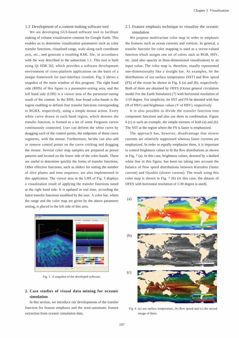
197


1.3 Development of a content making software toolWe are developing GUI-based software tool to facilitate

making of volume visualization contents for Google Earth. This enables us to determine visualization parameters such as color transfer functions, visualized range, scale along each coordinate axis, etc., and generate a resulting KML file, in accordance with the way described in the subsection 1.1. This tool is built using Qt SDK [6], which provides a software development environment of cross-platform applications on the basis of a unique framework for user-interface creation. Fig. 5 shows a snapshot of the main window of this program. The right hand side (RHS) of this figure is a parameter-setting area, and the left hand side (LHS) is a viewer area of the parameter-tuning result of the content. In the RHS, four broad color-bands is the region enabling to deform four transfer functions corresponding to RGBA, respectively, using a simple mouse action. Every white curve drawn in each band region, which denotes the transfer function, is formed as a set of some Ferguson curves continuously connected. User can deform the white curve by dragging each of the control points, the endpoints of those curve segments, with the mouse. Furthermore, he/she can also add or remove control points on the curve cricking and dragging the mouse. Several color map samples are prepared as preset patterns and located on the lower side of the color-bands. These are useful to determine quickly the forms of transfer functions. Other effective functions, such as sliders for setting the number of slice planes and time sequence, are also implemented in this application. The viewer area in the LHS of Fig. 5 displays a visualization result of applying the transfer functions tuned at the right hand side. It is updated in real time, according the latest transfer functions modified by the user. A color bar, where the range and the color map are given by the above parameter setting, is placed in the left side of this area.

Fig. 5 A snapshot of the developed software.

2. Case studies of visual data mining for oceanic simulationIn this section, we introduce our developments of the transfer

function for feature emphasis and the semi-automatic feature extraction from oceanic simulation data.

2.1. Feature emphasis technique to visualize the oceanic simulation

We propose multivariate color map in order to emphasis the features such as ocean currents and vortices. In general, a transfer function for color mapping is used as a vector-valued function which assigns one set of colors such as RGB, HSV, etc. (and also opacity in three-dimensional visualization) to an input value. The color map is, therefore, usually represented one-dimensionally like a straight bar. As examples, let the distributions of sea surface temperature (SST) and flow speed (FS) of the ocean be shown in Fig. 6 (a) and (b), respectively. Both of them are obtained by OFES (Ocean general circulation model For the Earth Simulator) [7] with horizontal resolution of 1/10 degree. For simplicity, let SST and FS be denoted with hue (H of HSV) and brightness values (V of HSV), respectively.

It is also possible to divide the transfer function into component functions and also use them in combination. Figure 6 (c) is such an example, the simple mixture of both (a) and (b). The SST at the region where the FS is faster is emphasized.

The approach has, however, disadvantage that slower currents are relatively suppressed whereas faster currents are emphasized. In order to equally emphasize them, it is important to control brightness values to fit the flow distributions as shown in Fig. 7 (a). In this case, brightness values, denoted by a dashed white line in this figure, has been set taking into account the balance of flow speed distributions between Kuroshio (faster current) and Oyashio (slower current). The result using this color map is shown in Fig. 7 (b) (in this case, the dataset of OFES with horizontal resolution of 1/30 degree is used).

Fig. 6 (a) sea surface temperature, (b) flow speed and (c) the mixed image of them.

(a)

(b)

(c)

198


2.2. Semi-automatic extraction of the ocean currentsAs a further approach in order to emphasize any currents

equally, we try to extract oceanic currents individually from the simulation data, using one of cluster analyses based on non-hierarchical algorithms. This approach clusters elements, each of which has an attribute, a set of values coming from several variables at a corresponding simulation grid point, into several groups. An initial cluster centroid of each group should be selected manually from those elements. A cluster consists of elements being regarded as mutually similar, beginning from the centroid. Therefore, one of the important steps is how to define similarity of the elements. We use a distance defined in the attribute space of the elements as a degree of the similarity.

In the trial, we selected four variables, a temperature, a current speed and position coordinates (latitude and longitude) as the attribute variables, and sixteen centroids on the latitude-longitude subspace as shown in Fig. 8. The result of this trial is shown by color-coding in the same figure. Not only typical currents such as the Kuroshio ((1) and (2)), the Kuroshio

extension region ((3) and (4)) and the Oyashio ((14) and (15)), but also the mixed layer in the Kuroshio/Oyashio extension region in the Sea of Japan are clustered almost correctly. In continuing this work, it is important to select the centroids and evaluate the clustering results.

SummaryThe EXTRAWING project was introduced. In this project,

one novel representation technique was proposed and two types of developed programs, the web application and the KML content-making tool were introduced. The web application has been public to general since December 2010. The content-making program is equipped a viewer and GUI for deforming transfer functions and effectively makes KML contents based on the proposed technique which laminates color contour images with opacity.

A multivariate color map to emphasize all of oceanic currents equally, taking into account flow speed distribution, was proposed. As the further approach, semi-automatic extraction of oceanic currents using one of cluster analyses based on non-hierarchical algorithms was also examined. Typical currents around Japan islands were successfully clustered almost correctly.

References[1] Google Earth, http://earth.google.com[2] KML, http://www.opengeospatial.org/standards/kml/[3] COLLADA, http://www.khronos.org/collada/[4] Google Earth API, http://code.google.com/intl/ja/apis/

earth/[5] Keiko Takahashi, Xindong Peng, Kenji Komine, Mitsuru

Ohdaira, Koji Goto, Masayuki Yamada, Hiromitsu Fuchigami, and Takeshi Sugimura, "Non-hydrostatic atmospheric GCM development and its computational performance", Use of High Performance computing in meteorology, Walter Zwieflhofer and George Mozdzynski Eds., World Scientific, pp. 50-62 (2005).

[6] Qt SDK, http://qt.nokia.com/[7] Y. Masumoto, H. Sasaki, T. Kagimoto, N. Komori,

A.Ishida, Y. Sasai, T. Miyama, T. Motoi, H. Mitsudera, K. Takahashi, H. Sakuma, and T. Yamagata, "A fifty-year eddy-resolving simulation of the world ocean: Preliminary outcomes of OFES (OGCM for the Earth Simulator)", J. Earth Simulator, Vol.1, pp. 35-56 (2004).

Fig. 8 Sixteen centroids and the resul t of non-hierarchical cluster analysis.

Fig. 7 (a) multivariate color map to emphasize the ocean currents and (b) the resulting image.

(a)

(b)

199


大規模データ可視化研究 : EXTRAWINGとビジュアルデータマイニング


荒木　文明　　海洋研究開発機構　地球シミュレータセンター

著者荒木　文明 *1，川原慎太郎 *1，松岡　大祐 *1，杉村　　剛 *1，馬場　雄也 *1，高橋　桂子 *1


地球シミュレータを用いた地球・環境流体シミュレーションによる結果を魅力的に表現し一般社会へ発信するプロジェクト、EXTRAWINGについて紹介する。EXTRAWINGは Google Earthをベースにしている。Google Earth上でシミュレーションデータの 3次元可視化表現と情報発信を可能にする、カラーコンター画像を層状に積み上げた流体場の分布の表現、社会へ向けた情報発信のためのWebアプリケーション開発、複雑なコンテンツを GUI上で容易に作成可能なツールの開発、について述べる。また、海洋シミュレーションのデータを用いて、特に海流の抽出をターゲットとしたビジュアルデータマイニングに

関する 2つの試みについて紹介する。ここでは、流速や水温の異なる複数の海流を多変数伝達関数によっていずれも同じ程度に強調する方法、およびクラスタ分析を用いた海流の半自動的な抽出法について述べる。

キーワード : EXTRAWING, Google Earth, Webアプリケーション , ツール開発 , 特徴抽出

Outline of the Earth Simulator Project

Documents

Transcript of Outline of the Earth Simulator Project