Assessment of the ECMWF Model Cloudiness and Surface Radiation Fields at the ARM SGP Site (2002)

FEBRUARY 2002 257M O R C R E T T E

q 2002 American Meteorological Society

Assessment of the ECMWF Model Cloudiness and Surface Radiation Fields at theARM SGP Site

JEAN-JACQUES MORCRETTE

European Centre for Medium-Range Weather Forecasts, Reading, United Kingdom

(Manuscript received 19 January 2001, in final form 18 June 2001)

ABSTRACT

The cloud and radiation fields produced by the operational ECMWF forecasts are assessed using observationsfrom the Atmospheric Radiation Measurement Program (ARM) Southern Great Plains (SGP) site over the April–May 1999 period. Over the first 36 h of the forecasts, most of the model fields, taken over a 24-h time window(either 0–24, 6–30, or 12–36 h) are generally in good agreement with each other. Comparisons of model fieldstaken from any such 24-h time window with observations are therefore representative of the quality of theECMWF model physical parameterizations. The surface radiation fluxes are assessed separately for clear-sky,overcast, and whole-sky situations. For clear-sky fluxes, differences between model and observations are linkedto differences in humidity and temperature profiles, the characterization of aerosols, and potential problems inthe radiation schemes. For clear-sky conditions, the downward longwave radiation is usually within the accuracyof the measurements. For overcast conditions, the agreement with observations is also usually good. On theother hand, the downward shortwave radiation is overestimated, whatever the conditions. Although this mightbe partly due to uncertainties in the aerosol content, the clear-sky overestimation of the downward shortwaveradiation, when aerosols are specified from climatic values or observations, indicates an underestimation of thegaseous absorption. Model cloud occurrences and boundaries over the SGP Central Facility are compared withsimilar quantities derived from radar and micropulse lidar observations. Model cloud water is tentatively assessedthrough comparisons with the radar reflectivity measurements. Systematic deficiencies in the surface radiationfields in the presence of clouds are discussed with respect to differences between the model and observed cloudcharacteristics. Given the TL319 resolution of the ECMWF model at the time of the comparisons, both the day-to-day and within-the-day temporal variability are captured reasonably well by 24-h forecasts that include cloud–radiation interactions with 1-h time resolution. However, most of the differences with observations can be tracedback either to deficiencies in the clear-sky shortwave radiation scheme or to problems in the cloud fraction and/or cloud water content.

1. Introduction

The top-of-the atmosphere (TOA) radiation longwave(LW) and shortwave (SW) radiation fields produced bygeneral circulation models (GCMs) have been assessedglobally since, in the mid-1960s, satellites started tomeasure radiances [e.g., Holloway and Manabe (1971)using the radiation budget from Vonder Haar (1969)].Contrary to TOA radiation, an assessment for surfaceradiation fields has appeared much more recently withthe production of the first satellite-derived surface ra-diation climatologies (Darnell et al. 1992; Laszlo andPinker 1993; Li and Leighton 1993). Even so, the qual-ity of such surface radiation climatologies is still ques-tioned, because of processes either inadequately knownand/or accounted for in the retrieval (LW absorption bythe water vapor continuum, LW and SW aerosol effects,‘‘anomalous’’ SW absorption).

Corresponding author address: Dr. Jean-Jacques Morcrette, ECMWF,Shinfield Park, Reading, Berkshire RG2 9AX, United Kingdom.E-mail: [email protected]

In the recent past, good-quality surface radiation mea-surements such as those screened from the Global En-ergy Balance Archive (Ohmura and Gilgen 1993) haveusually been preferred for the evaluation of the surfaceradiation fields produced by GCMs. Garratt and coau-thors (Garratt 1994; Garratt and Prata 1996; Garratt etal. 1998), and Wild and coauthors (Wild et al. 1995,1998a,b, 2000) have looked at the biases produced byGCMs and operational analyses and at their implicationsfor climate modeling. However, such studies are usuallycarried out on a monthly timescale, with a mix of clear-sky and cloudy conditions. Distinctions between sys-tematic and random errors have not been clearly stated:the deficiencies in the surface radiation fields identifiedby these studies have not been readily ascribed, in thecase of noncloudy situations, to model deficiencies inthe radiation codes, in temperature and humidity pro-files, or to the improper or lack of accounting for aero-sols. In the case of cloudy situations, the deficienciespreviously noted have been inadequately characterizedin terms of the cloudiness produced by the model (i.e.,

258 VOLUME 130M O N T H L Y W E A T H E R R E V I E W

TABLE 1. Observational data used in this study: Central Facility.

Observational system AcronymObserved/retrievedphysical quantities

Original datafrequency

Atmospheric emitted radiance interferome-ter

AERI Planetary boundary layer temperature andwater vapor profiles

;480 s

Belfort laser ceilometer BLC Base height of lowest cloud 30 sEnergy balance Bowen ratio EBBR Air temperature and relative humidity,

soil temperature, net radiation, surfacepressure

1800 s

Geostationary Operational EnvironmentalSatellite-8

GOES-8 Radiances at 3.9, 6.9, 10.9 and 11.6 mm;retrieved temperature and dewpoint

30 min–2 h

Micropulse lidar MPL Cloud boundaries ;60 sMultifilter rotating shadowband radiometer MFRSR Aerosol optical thickness ;60 sMultimode cloud radar MMCR Cloud boundaries, mask, and reflectivity 10 sMicrowave radiometer MWR Vertically integrated amounts of water va-

por and cloud liquid water20 s

Solar–Infrared radiation stations SIRS Up- and downwelling longwave andshortwave radiation

60 s

Radiosonde SONDE Temperature and dewpoint profiles 2–4 dailySurface meteorological observation system SMOS Air temperature and relative humidity,

surface pressure, precipitation1800 s

cloud fraction, cloud-base height, optical thickness,cloud condensed water). Moreover, in these compari-sons, the information about these profiles is usually in-complete, so that a thorough assessment is difficult.

In the past, a number of in situ measurement cam-paigns have provided simultaneous observations ofsome of the cloud–radiation-related parameters over agiven location, usually over a rather short period of time.These measurements unfortunately have not been usedgenerally to assess the quality of the model simulationsand operational analyses.

The much wider set of observations of the Atmo-spheric Radiation Measurement Program (ARM; Stokesand Schwartz 1994) provides better definition of thesurface radiation budget and its governing parameters,allowing more constraints in the verification of the fieldsproduced by a large-scale model (Beesley et al. 2000;Mace et al. 2000). In this study, two months of mea-surements over the ARM Southern Great Plains site(SGP) in Oklahoma are used to evaluate most of thecloud-radiation aspects in the European Centre for Me-dium-Range Weather Forecasts (ECMWF) model. Theobservational and model data are discussed in section2. Results for the model grid point corresponding to theSGP Central Facility (CF) are presented in section 3.The sensitivity of the surface radiation fields to detailsof the parameterization is presented in section 4. Dis-cussion and conclusions are presented in section 5.

2. Methodology

a. Observational and model data

The study covers the whole months of April and Mayof 1999. A spring period was preferred because springhad, in the past, not been a particularly good period forECMWF forecasts. Moreover, for somewhat average con-ditions of temperature and humidity, a large temporal var-

iability can be expected at the latitude of the ARM SGPsite (Lamont, Oklahoma, 36.6058N, 97.4858W), dependingon the flow direction of the prevalent air mass. In thefollowing, use is made of measurements by the obser-vational systems located at the CF. These are defined to-gether with the measured parameters in Table 1.

The ECMWF fields correspond to outputs every hourfor all 36-h forecasts starting 24 h apart between 1200UTC 31 March 1999 and 1200 UTC 31 May 1999. Theanalyses from which the forecasts were started are ob-tained through a 4D variational assimilation of all theobservations during a 6-h window centered around theanalysis time (Rabier et al. 1998; Mahfouf and Rabier2000). The model used in this study is the so-calledcycle 23R1 of the ECMWF Integrated Forecast System,operational between 27 June and 11 November 2000.Among the modifications introduced with cycle 23R1are the replacement of the previous longwave scheme[based on Morcrette (1991), and described in Gregoryet al. (2000, hereinafter referred to as G00)] by the RapidRadiation Transfer Model (RRTM; Mlawer et al. 1997)and the introduction of a tiling scheme for the surfaceprocesses (van den Hurk et al. 2000). The G00 LWscheme included cloud effects using maximum-randomoverlap of effective cloud layers through an effectiveemissivity approach. The ECMWF version of the RRTMLW scheme (Morcrette et al. 1998) also includes a max-imum-random overlap assumption but keeps the cloudfraction and cloud optical thickness as two separatequantities.

The rest of the package of physical parameterizations(Gregory et al. 2000) includes the SW radiation schemeoriginally developed by Fouquart and Bonnel (1980)and revised by Morcrette (1993). The cloud opticalproperties are based on Ebert and Curry (1992) for iceclouds and on Fouquart (1987) and Smith and Shi (1992)for water clouds. All cloudy fluxes are computed from


cloud optical thicknesses derived from the prognosedliquid and ice cloud water content weighted by a 0.7inhomogeneity factor following Tiedtke (1996). Theswitching between deep or shallow convection wasmodified in December of 1997 (cycle 18R6) from a teston the moisture convergence to one based on the depthof the convection (Gregory et al. 2000). The dynamicalpart of the model includes the two-time-level semi-La-grangian scheme (Temperton et al. 2001) on a lineargrid similar to that used in Hortal and Simmons (1991).

The prognostic cloud scheme (Tiedtke 1993) repre-sents both stratiform and convective clouds, and theirtime evolution is defined through two large-scale budgetequations for cloud water content and cloud fractionalcover. This scheme links the formation of clouds tolarge-scale ascent, diabatic cooling, boundary layer tur-bulence, and their dissipation to adiabatic and diabaticheating, turbulent mixing of cloud air with unsaturatedenvironmental air, and precipitation processes. The re-sults presented in the following sections are obtainedwith the scheme used operationally for global forecastsand analyses. It includes the original formulation of thefallout of cloud ice of Tiedtke (1993). It only differsfrom Tiedtke’s original formulation through a new pre-cipitation/evaporation method (Jakob and Klein 2000),which explicitly accounts for the vertical distribution ofcloud layers and allows the cloud overlap assumptionto be applied consistently with what is done for theradiative computations.

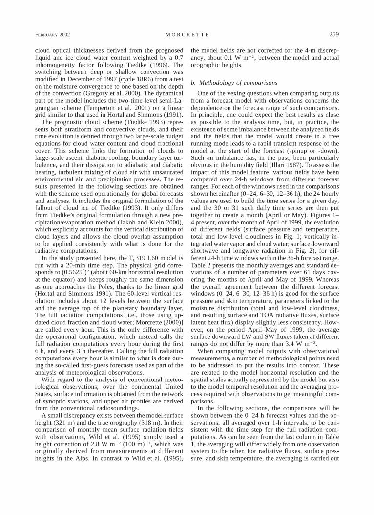
In the study presented here, the TL319 L60 model isrun with a 20-min time step. The physical grid corre-sponds to (0.56258)2 (about 60-km horizontal resolutionat the equator) and keeps roughly the same dimensionas one approaches the Poles, thanks to the linear grid(Hortal and Simmons 1991). The 60-level vertical res-olution includes about 12 levels between the surfaceand the average top of the planetary boundary layer.The full radiation computations [i.e., those using up-dated cloud fraction and cloud water; Morcrette (2000)]are called every hour. This is the only difference withthe operational configuration, which instead calls thefull radiation computations every hour during the first6 h, and every 3 h thereafter. Calling the full radiationcomputations every hour is similar to what is done dur-ing the so-called first-guess forecasts used as part of theanalysis of meteorological observations.

With regard to the analysis of conventional meteo-rological observations, over the continental UnitedStates, surface information is obtained from the networkof synoptic stations, and upper air profiles are derivedfrom the conventional radiosoundings.

A small discrepancy exists between the model surfaceheight (321 m) and the true orography (318 m). In theircomparison of monthly mean surface radiation fieldswith observations, Wild et al. (1995) simply used aheight correction of 2.8 W m22 (100 m)21, which wasoriginally derived from measurements at differentheights in the Alps. In contrast to Wild et al. (1995),

the model fields are not corrected for the 4-m discrep-ancy, about 0.1 W m22, between the model and actualorographic heights.

b. Methodology of comparisons

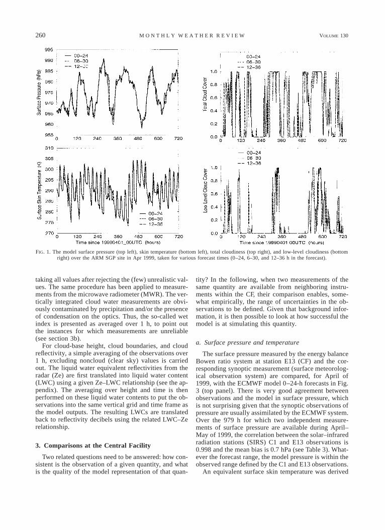
One of the vexing questions when comparing outputsfrom a forecast model with observations concerns thedependence on the forecast range of such comparisons.In principle, one could expect the best results as closeas possible to the analysis time, but, in practice, theexistence of some imbalance between the analyzed fieldsand the fields that the model would create in a freerunning mode leads to a rapid transient response of themodel at the start of the forecast (spinup or -down).Such an imbalance has, in the past, been particularlyobvious in the humidity field (Illari 1987). To assess theimpact of this model feature, various fields have beencompared over 24-h windows from different forecastranges. For each of the windows used in the comparisonsshown hereinafter (0–24, 6–30, 12–36 h), the 24 hourlyvalues are used to build the time series for a given day,and the 30 or 31 such daily time series are then puttogether to create a month (April or May). Figures 1–4 present, over the month of April of 1999, the evolutionof different fields (surface pressure and temperature,total and low-level cloudiness in Fig. 1; vertically in-tegrated water vapor and cloud water; surface downwardshortwave and longwave radiation in Fig. 2), for dif-ferent 24-h time windows within the 36-h forecast range.Table 2 presents the monthly averages and standard de-viations of a number of parameters over 61 days cov-ering the months of April and May of 1999. Whereasthe overall agreement between the different forecastwindows (0–24, 6–30, 12–36 h) is good for the surfacepressure and skin temperature, parameters linked to themoisture distribution (total and low-level cloudiness,and resulting surface and TOA radiative fluxes, surfacelatent heat flux) display slightly less consistency. How-ever, on the period April–May of 1999, the averagesurface downward LW and SW fluxes taken at differentranges do not differ by more than 3.4 W m22.

When comparing model outputs with observationalmeasurements, a number of methodological points needto be addressed to put the results into context. Theseare related to the model horizontal resolution and thespatial scales actually represented by the model but alsoto the model temporal resolution and the averaging pro-cess required with observations to get meaningful com-parisons.

In the following sections, the comparisons will beshown between the 0–24 h forecast values and the ob-servations, all averaged over 1-h intervals, to be con-sistent with the time step for the full radiation com-putations. As can be seen from the last column in Table1, the averaging will differ widely from one observationsystem to the other. For radiative fluxes, surface pres-sure, and skin temperature, the averaging is carried out


FIG. 1. The model surface pressure (top left), skin temperature (bottom left), total cloudiness (top right), and low-level cloudiness (bottomright) over the ARM SGP site in Apr 1999, taken for various forecast times (0–24, 6–30, and 12–36 h in the forecast).

taking all values after rejecting the (few) unrealistic val-ues. The same procedure has been applied to measure-ments from the microwave radiometer (MWR). The ver-tically integrated cloud water measurements are obvi-ously contaminated by precipitation and/or the presenceof condensation on the optics. Thus, the so-called wetindex is presented as averaged over 1 h, to point outthe instances for which measurements are unreliable(see section 3b).

For cloud-base height, cloud boundaries, and cloudreflectivity, a simple averaging of the observations over1 h, excluding noncloud (clear sky) values is carriedout. The liquid water equivalent reflectivities from theradar (Ze) are first translated into liquid water content(LWC) using a given Ze–LWC relationship (see the ap-pendix). The averaging over height and time is thenperformed on these liquid water contents to put the ob-servations into the same vertical grid and time frame asthe model outputs. The resulting LWCs are translatedback to reflectivity decibels using the related LWC–Zerelationship.

3. Comparisons at the Central Facility

Two related questions need to be answered: how con-sistent is the observation of a given quantity, and whatis the quality of the model representation of that quan-

tity? In the following, when two measurements of thesame quantity are available from neighboring instru-ments within the CF, their comparison enables, some-what empirically, the range of uncertainties in the ob-servations to be defined. Given that background infor-mation, it is then possible to look at how successful themodel is at simulating this quantity.

a. Surface pressure and temperature

The surface pressure measured by the energy balanceBowen ratio system at station E13 (CF) and the cor-responding synoptic measurement (surface meteorolog-ical observation system) are compared, for April of1999, with the ECMWF model 0–24-h forecasts in Fig.3 (top panel). There is very good agreement betweenobservations and the model in surface pressure, whichis not surprising given that the synoptic observations ofpressure are usually assimilated by the ECMWF system.Over the 979 h for which two independent measure-ments of surface pressure are available during April–May of 1999, the correlation between the solar–infraredradiation stations (SIRS) C1 and E13 observations is0.998 and the mean bias is 0.7 hPa (see Table 3). What-ever the forecast range, the model pressure is within theobserved range defined by the C1 and E13 observations.

An equivalent surface skin temperature was derived


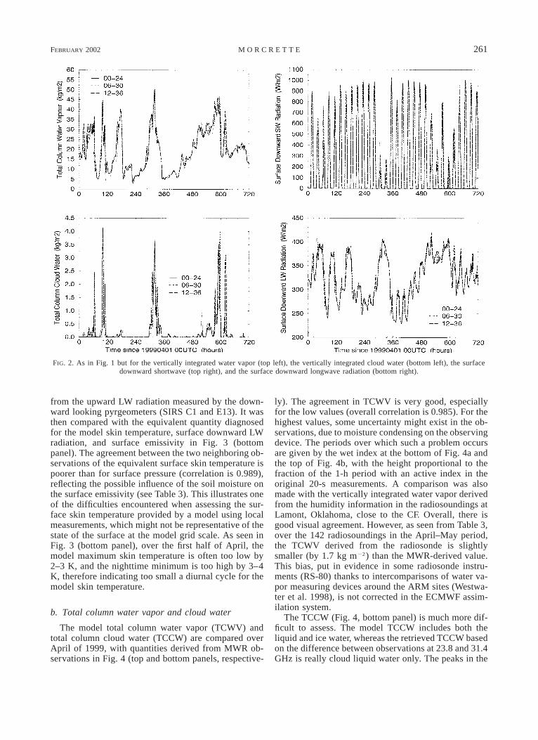
FIG. 2. As in Fig. 1 but for the vertically integrated water vapor (top left), the vertically integrated cloud water (bottom left), the surfacedownward shortwave (top right), and the surface downward longwave radiation (bottom right).

from the upward LW radiation measured by the down-ward looking pyrgeometers (SIRS C1 and E13). It wasthen compared with the equivalent quantity diagnosedfor the model skin temperature, surface downward LWradiation, and surface emissivity in Fig. 3 (bottompanel). The agreement between the two neighboring ob-servations of the equivalent surface skin temperature ispoorer than for surface pressure (correlation is 0.989),reflecting the possible influence of the soil moisture onthe surface emissivity (see Table 3). This illustrates oneof the difficulties encountered when assessing the sur-face skin temperature provided by a model using localmeasurements, which might not be representative of thestate of the surface at the model grid scale. As seen inFig. 3 (bottom panel), over the first half of April, themodel maximum skin temperature is often too low by2–3 K, and the nighttime minimum is too high by 3–4K, therefore indicating too small a diurnal cycle for themodel skin temperature.

b. Total column water vapor and cloud water

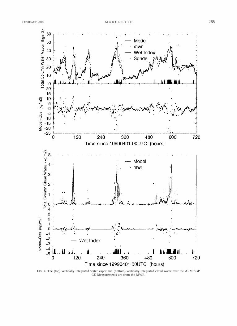
The model total column water vapor (TCWV) andtotal column cloud water (TCCW) are compared overApril of 1999, with quantities derived from MWR ob-servations in Fig. 4 (top and bottom panels, respective-

ly). The agreement in TCWV is very good, especiallyfor the low values (overall correlation is 0.985). For thehighest values, some uncertainty might exist in the ob-servations, due to moisture condensing on the observingdevice. The periods over which such a problem occursare given by the wet index at the bottom of Fig. 4a andthe top of Fig. 4b, with the height proportional to thefraction of the 1-h period with an active index in theoriginal 20-s measurements. A comparison was alsomade with the vertically integrated water vapor derivedfrom the humidity information in the radiosoundings atLamont, Oklahoma, close to the CF. Overall, there isgood visual agreement. However, as seen from Table 3,over the 142 radiosoundings in the April–May period,the TCWV derived from the radiosonde is slightlysmaller (by 1.7 kg m22) than the MWR-derived value.This bias, put in evidence in some radiosonde instru-ments (RS-80) thanks to intercomparisons of water va-por measuring devices around the ARM sites (Westwa-ter et al. 1998), is not corrected in the ECMWF assim-ilation system.

The TCCW (Fig. 4, bottom panel) is much more dif-ficult to assess. The model TCCW includes both theliquid and ice water, whereas the retrieved TCCW basedon the difference between observations at 23.8 and 31.4GHz is really cloud liquid water only. The peaks in the


TABLE 2. Comparison of model quantities for different ranges within the forecasts over the Apr–May 1999 period. Values are the timeaverages of the various parameters and, in parentheses, the corresponding standard deviation.

Unit 000–024 h 006–030 h 012–036 h

Surface pressureSkin temperatureSurface albedoTotal cloud coverLow-level cloudinessColumn water vaporColumn cloud water

hPaK%%%kg m22

g m22

975.2291.714.7638.915.221.7

162

(7.0)(6.5)(0.002)(0.4)(0.3)

(10.0)(11)

975.1291.814.7638.814.221.9

168

(7.0)(6.6)(0.002)(0.4)(0.3)

(10.2)(12)

975.1291.714.7640.414.922.2

185

(6.9)(6.6)(0.002)(0.4)(0.3)

(10.3)(13)

Soil moistureDownward SW fluxDownward LW fluxLatent heat fluxSensible heat fluxTOA net SW fluxTOA outgoing LW flux

mmW m22

W m22

W m22

W m22

W m22

W m22

292258.1339.8119.621.1

320.4260.3

(35)(329.6)(46.1)

(137.6)(95.0)

(371.9)(29.6)

291260.0339.6121.320.6

321.9259.6

(35)(331.3)(46.1)

(139.3)(94.3)

(373.2)(29.8)

292259.2339.4121.920.5

321.5258.3

(36)(333.0)(45.8)

(141.3)(94.6)

(374.2)(30.5)

observations obviously correspond to clouds above theMWR. They are also usually flagged as wet, so theobservations are likely to include precipitation.

c. Downward radiation

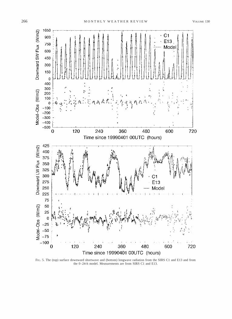
The corresponding surface downward SW and LWradiation are presented in Fig. 5 (top panel for surfacedownward SW; bottom panel for surface downward LW)as measured from two sets of radiometers located at theCF (C1 and E13) and as represented by the model fore-casts. Table 3 presents the regression statistics betweenthese two sets of measurements over the April–Mayperiod. For all the time slots for which both the E13and C1 measurements are available over the April–Mayperiod, the correlation between the two stations is betterthan 0.999 for both the surface downward SW and sur-face downward LW radiation. Some uncertainty arisesfrom the (small) negative values usually reported by thepyranometers at night. In Table 3, statistics for the sur-face downward SW are reported three times, the firstset corresponding to all observations during the period,the second set to all observations with nighttime valuesset to zero, and the third set to daytime observationsonly. Over the 2-month period of the observations, thedifference between the first two approaches is at most2.5 W m22. In both cases, the correlation is practicallyunity, and the slope is higher than 0.998. Therefore, theslight disagreement between these two approaches isunlikely to be of concern for evaluating the model be-havior.

In a clear-sky atmosphere, the surface downward LWis mostly between 240 and 290 W m22. Only whenclouds are present does the surface downward LW getover 300 W m22, with the values over 360 W m22

corresponding to the presence of low-level cloudiness.There is a reasonable agreement between model andobserved surface downward LW (see Fig. 7, bottompanel, below), reflecting the ability of the model to pro-duce the cloud events at the right time, with cloud baseclose to the proper height. A more detailed assessment

of the behavior of the schemes in clear-sky and cloudyconditions is carried out next.

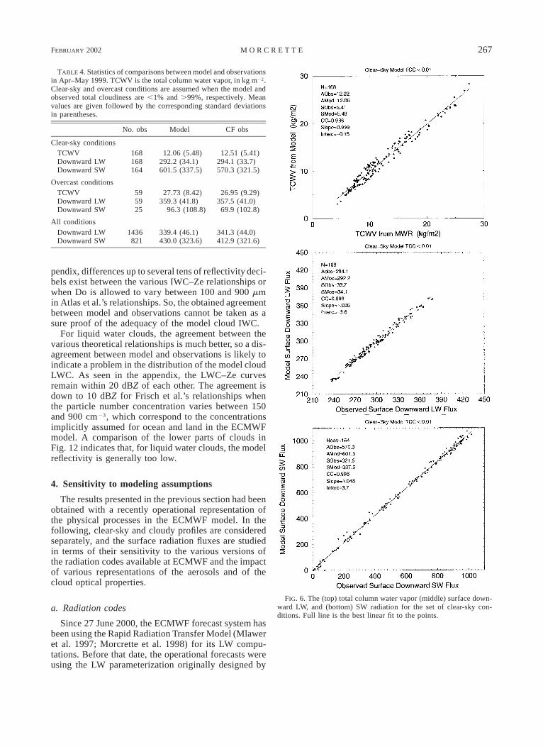
From the 1464 (61 days 3 24) 1-h slots in April–May of 1999, 168 clear-sky situations have been ex-tracted (only 164 such situations are for daytime con-ditions and thus are used for the SW). This extractionis based on the following set of conditions: a modeltotal cloud cover of less than 1%, no return from themultimode cloud radar (MMCR), no cloud base fromthe micropulse lidar (MPL), and a zero wet index fromthe MWR. Table 4 presents the statistics of the com-parisons for the TCWV, surface downward LW, and sur-face downward SW. Over this set of profiles, there is avery good agreement between the MWR-observed andmodel TCWV and surface downward LW (Fig. 6). Theagreement for the surface downward LW is within therange obtained when comparing C1 and E13 SIRS mea-surements. In contrast, even for these selected clear-skycases, the model surface downward SW overestimatesthe observed surface downward SW by 31.2 W m22

over the 164 daytime situations. This reflects a likelybias in the SW radiation scheme or an improper spec-ification of the aerosol optical thickness (see section 4).

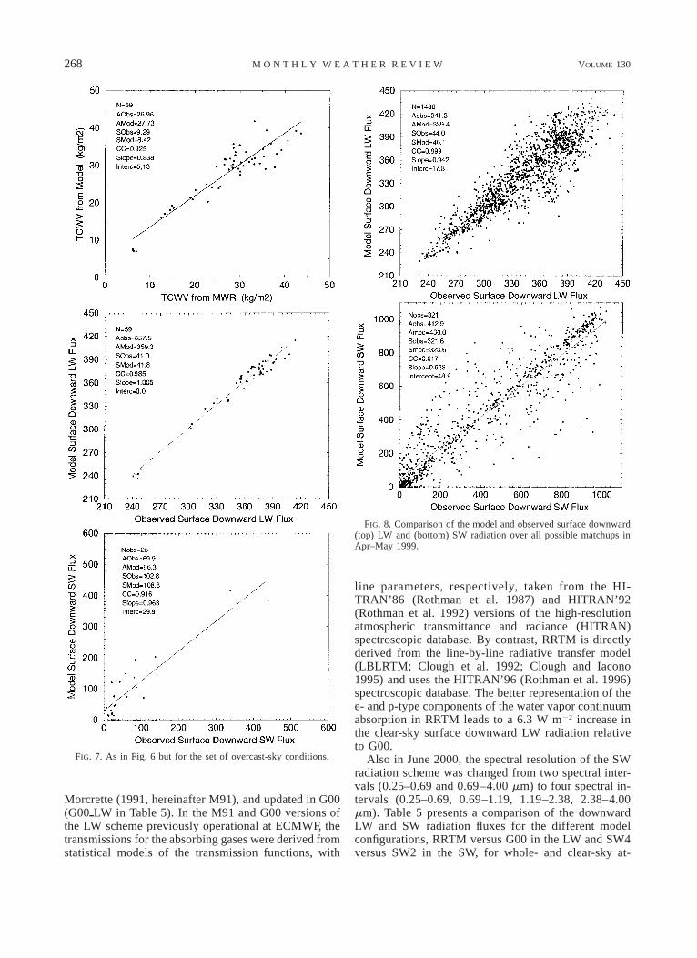
In the presence of cloudiness, the discrepancies be-tween model and observed surface radiation fluxes areas likely to come from incorrect atmospheric profiles orincorrect definition of the cloud parameters (cloud-baseheight and optical properties) produced by the forecastsas from the radiation schemes used in the model. There-fore a set of 59 overcast situations (25 during daytimeare used for the surface downward SW) has been ex-tracted, for which the model total cloud cover is greaterthan 99%, with the presence of clouds during all inter-vals composing the 1-h slot in the MMCR, Belfort laserceilometer (BLC), and MPL observations. Results arepresented in Fig. 7. These cases show agreement onboth the cloud cover and the cloud-base height. How-ever, the comparison between MWR-observed and mod-el TCWV is certainly affected by moisture condensating(dew) or precipitating on the observing device. Theagreement in surface downward LW is again good (with


FIG. 3. The (top) surface pressure and (bottom) surface skin temperature over the ARM SGP Central Facility.Measurements are from the energy balance Bowen ratio system and synoptic measurements for pressure and are derivedfrom SIRS C1 and E13 for skin temperature.

a 2 W m22 model overestimation). Again, the modelsurface downward SW overestimates the observed sur-face downward SW by 26.4 W m22. The overestimationis consistent with the deficiency already seen for the

SW radiation scheme in clear-sky conditions, but prob-lems in the definition of the cloud optical parameters(optical thickness in particular) cannot be ruled out andare as likely to increase as decrease the clear-sky error.


TABLE 3. Statistics for measurements at two neighboring locationsover the Apr–May period. TCWV is the vertically integrated watervapor (total column water vapor, kg m22). Statistics for the surfacedownward SW radiation are given averaged over all measurements,averaged over all measurements setting the (slightly negative) night-time values to zero (see text), and averaged over daytime only. Incolumns C1 and E13, mean values are given followed by the cor-responding standard deviations in parentheses.

No. obs C1 E13

Surface pressure 979 974.6 (6.4) 975.3 (6.4)Skin temperature 979 291.0 (6.8) 291.4 (7.0)TCWV 142 20.3 (8.3) 18.6 (7.9)Downward SW 1068 249.4 (329.9)

251.4 (328.2)247.9 (329.6)250.4 (327.4)

603 445.6 (323.1) 443.8 (322.8)Downward LW 1075 337.6 (47.4) 340.7 (47.1)

Figure 8 displays the comparisons between model andobserved downward radiation over the two months. Thelast two lines in Table 4 give the corresponding statisticsfor all possible comparisons for surface radiation overthe two months. Over the 1436 LW comparisons (Fig.8, top panel), the model underestimates the observationsby 2 W m22. The SW comparisons (Fig. 8, bottompanel) are restricted to 821 daytime comparisons andshow a 17 W m22 overestimation by the model. Evenfor LW, for which the agreement between model andobservations is good in clear-sky and overcast condi-tions, the visual impression in Fig. 8 is of a deteriorationof the agreement for all possible matchups in April–May of 1999. Although the average values for modeland observed surface downward LW are still within 2W m22, there is a large scatter mainly related to a mixof differences in the exact occurrence of cloudiness overthe site, in the cloud amount and cloud-base height, andin the cloud optical thickness/emissivity. Note that, overthe ARM SGP site during the April–May 1999 period,only 15% (23%) of the situations over the two monthsare either clear-sky or overcast situations for both themodel and the observations and, as such, conducive todirect LW (SW) comparisons.

The net radiation (SWdown 2 SWup 1 LWdown 2LWup), as produced by the model, was also comparedwith the net radiation measured by the energy balanceBowen ratio system at station E13 (not shown). In themodel, the often large overestimation of the surfacedownward SW, the slight underestimation of surfacedownward LW, and the too-large skin temperature atnight all contribute to the signature. The model producestoo much energy input to the surface during daytimeand too much energy output from the surface at night.

d. Cloudiness

The temperature and humidity in the first 3000 mabove the surface are presented for the ECMWF modeland are derived from the atmospheric emitted radianceinterferometer (AERI) in Figs. 9 and 10, over April andMay of 1999. For individual profiles (not shown), there

is an overall good agreement between model and ob-servations, with the range of differences going from211.0 to 11.6 K for temperature and from 25.2 to 8.3g kg21 for humidity. However, the average bias over thefirst 3000 m of the atmosphere varies between 1.4 K atthe surface and 21.5 K at 3000 m for temperature, andbetween 0.3 g kg21 between 300 and 800 m and 20.3g kg21 around 2000 m. Overall, the model suffers froma small warm bias in the lower kilometer accompaniedby a slightly larger one above. The humidity follows asimilar pattern.

The capability of the ECMWF model to producecloudiness at the proper time and height can be alsojudged by comparing the model cloud fraction with aso-called cloud mask produced from radar measure-ments and/or the height of clouds detected by the MPLor the BLC. When a large amount of cloud, with sub-stantial low-level cloudiness, is present (2–3, 7, 13–14,24–25 April), the agreement for cloud-base height be-tween BLC measurements and the model is generallygood (not shown). At other times, the agreement is muchpoorer, and the cloudiness derived from MMCR mea-surements often does not support the BLC measure-ments. The vertical distribution of clouds produced bythe ECMWF model forecasts for April of 1999 wascompared with the cloud mask derived from MMCRand MPL measurements using Clothiaux et al.’s (1995)algorithm (not shown). Another cloud mask derivedfrom MMCR measurements using Campbell et al.’s(1998) algorithm was also compared with the model andwas found to lead to similar conclusions.

The vertical distribution of the model cloud ice andliquid water content is presented in Figs. 11a and 11b,respectively. In the ECMWF model, the distinction be-tween liquid and ice water is made based on temperatureusing a relationship developed by Matveev (1984). Itincludes a mixed phase between 08 and 2238C, seen asan overlap between the two distributions in Fig. 11.

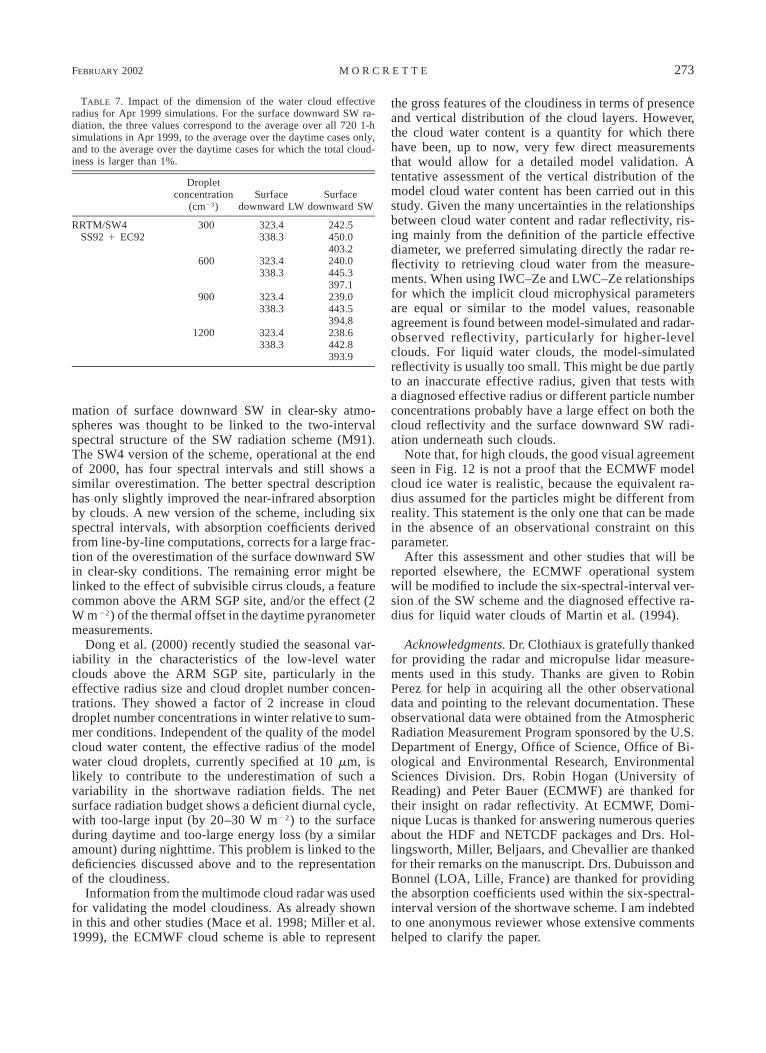
A Ze reflectivity simulated using ice water content(IWC)–Ze and LWC–Ze relationships from the modelIWC and LWC fields of Fig. 11 is presented in Fig. 12(top panel). Details of the procedure follow those ofBeesley et al. (2000) and are given in the appendix. Thecorresponding Ze reflectivity derived from MMCR mea-surements by Clothiaux et al. (2000) is presented in thebottom panel of Fig. 12. The effect of heavy precipi-tation on the radar reflectivity data can be seen on 2, 7,13, and 24 April. The observed reflectivity saturates atthese times corresponding to a wet index of 1 in theMWR measurements.

The comparison of the two panels in Fig. 12 showsthat, in terms of reflectivity, the model is in the ballparkof the measurements, particularly for the higher-level(ice) clouds. The results are obtained using the IWC–Ze relationship of Atlas et al. (1995) for a 100-mmequivalent particle diameter Do, within the range 60–120 mm diagnosed by the model from temperature, fol-lowing Matveev (1984). However, as seen in the ap-


FIG. 4. The (top) vertically integrated water vapor and (bottom) vertically integrated cloud water over the ARM SGPCF. Measurements are from the MWR.


FIG. 5. The (top) surface downward shortwave and (bottom) longwave radiation from the SIRS C1 and E13 and fromthe 0–24-h model. Measurements are from SIRS C1 and E13.


TABLE 4. Statistics of comparisons between model and observationsin Apr–May 1999. TCWV is the total column water vapor, in kg m22.Clear-sky and overcast conditions are assumed when the model andobserved total cloudiness are ,1% and .99%, respectively. Meanvalues are given followed by the corresponding standard deviationsin parentheses.

No. obs Model CF obs

Clear-sky conditionsTCWVDownward LWDownward SW

168168164

12.06 (5.48)292.2 (34.1)601.5 (337.5)

12.51 (5.41)294.1 (33.7)570.3 (321.5)

Overcast conditionsTCWVDownward LWDownward SW

595925

27.73 (8.42)359.3 (41.8)

96.3 (108.8)

26.95 (9.29)357.5 (41.0)69.9 (102.8)

All conditionsDownward LWDownward SW

1436821

339.4 (46.1)430.0 (323.6)

341.3 (44.0)412.9 (321.6)

FIG. 6. The (top) total column water vapor (middle) surface down-ward LW, and (bottom) SW radiation for the set of clear-sky con-ditions. Full line is the best linear fit to the points.

pendix, differences up to several tens of reflectivity deci-bels exist between the various IWC–Ze relationships orwhen Do is allowed to vary between 100 and 900 mmin Atlas et al.’s relationships. So, the obtained agreementbetween model and observations cannot be taken as asure proof of the adequacy of the model cloud IWC.

For liquid water clouds, the agreement between thevarious theoretical relationships is much better, so a dis-agreement between model and observations is likely toindicate a problem in the distribution of the model cloudLWC. As seen in the appendix, the LWC–Ze curvesremain within 20 dBZ of each other. The agreement isdown to 10 dBZ for Frisch et al.’s relationships whenthe particle number concentration varies between 150and 900 cm23, which correspond to the concentrationsimplicitly assumed for ocean and land in the ECMWFmodel. A comparison of the lower parts of clouds inFig. 12 indicates that, for liquid water clouds, the modelreflectivity is generally too low.

4. Sensitivity to modeling assumptions

The results presented in the previous section had beenobtained with a recently operational representation ofthe physical processes in the ECMWF model. In thefollowing, clear-sky and cloudy profiles are consideredseparately, and the surface radiation fluxes are studiedin terms of their sensitivity to the various versions ofthe radiation codes available at ECMWF and the impactof various representations of the aerosols and of thecloud optical properties.

a. Radiation codes

Since 27 June 2000, the ECMWF forecast system hasbeen using the Rapid Radiation Transfer Model (Mlaweret al. 1997; Morcrette et al. 1998) for its LW compu-tations. Before that date, the operational forecasts wereusing the LW parameterization originally designed by


FIG. 7. As in Fig. 6 but for the set of overcast-sky conditions.

FIG. 8. Comparison of the model and observed surface downward(top) LW and (bottom) SW radiation over all possible matchups inApr–May 1999.

Morcrette (1991, hereinafter M91), and updated in G00(G00pLW in Table 5). In the M91 and G00 versions ofthe LW scheme previously operational at ECMWF, thetransmissions for the absorbing gases were derived fromstatistical models of the transmission functions, with

line parameters, respectively, taken from the HI-TRAN’86 (Rothman et al. 1987) and HITRAN’92(Rothman et al. 1992) versions of the high-resolutionatmospheric transmittance and radiance (HITRAN)spectroscopic database. By contrast, RRTM is directlyderived from the line-by-line radiative transfer model(LBLRTM; Clough et al. 1992; Clough and Iacono1995) and uses the HITRAN’96 (Rothman et al. 1996)spectroscopic database. The better representation of thee- and p-type components of the water vapor continuumabsorption in RRTM leads to a 6.3 W m22 increase inthe clear-sky surface downward LW radiation relativeto G00.

Also in June 2000, the spectral resolution of the SWradiation scheme was changed from two spectral inter-vals (0.25–0.69 and 0.69–4.00 mm) to four spectral in-tervals (0.25–0.69, 0.69–1.19, 1.19–2.38, 2.38–4.00mm). Table 5 presents a comparison of the downwardLW and SW radiation fluxes for the different modelconfigurations, RRTM versus G00 in the LW and SW4versus SW2 in the SW, for whole- and clear-sky at-


FIG. 9. The temperature in the first 3000 m derived from theECMWF model 0–24-h forecasts. Statistics are computed over theperiod Apr–May 1999 for the 1013 1-h slots when AERI-derivedtemperature profiles are available. The bias is the difference model2 observations. The standard deviations of the model and observedtemperatures are plotted multiplied by 10. Unit is degrees Celsius.

FIG. 10. The humidity in the first 3000 m derived from the ECMWFmodel 0–24-h forecasts. Statistics are computed over the period Apr–May 1999 for the 1013 1-h slots when AERI-derived humidity profilesare available. The bias is the difference model 2 observations. Thestandard deviations of the model and observed humidity are plottedmultiplied by 10. Unit is grams per kilogram.

mospheres. The impact of changing the number of spec-tral intervals (from four to two) in the near-infrared partof the spectrum is very small for clear-sky SW radiation(a 0.4 W m22 decrease in the daytime-only average).The impact is larger for cloudy conditions (22 W m22

when averaged over daytime only). A new version ofthe SW scheme, SW6, based on line-by-line computa-tions from more recent spectroscopic data (Rothman etal. 1996) and including a proper separation of the UVand visible band is under development. Results in Table5 show it to correct for a large fraction of the overes-timation of the surface downward SW in clear-sky con-ditions.

b. Representation of aerosols

The ECMWF model is operationally run with an an-nually averaged climatological distribution of aerosols,first designed by Tanre et al. (1984). In the current modelconfiguration, five types of aerosols are considered, fourwith a geographical variation (maritime, continental, ur-ban, and desert aerosols); the fifth one, a stratosphericbackground aerosol, is included with a homogeneous hor-izontal distribution. Table 5 presents the effect of thisclimatological aerosol on the downward flux above theARM SGP site. With both the pre– and the post–27 Juneradiation codes (pre, G00pLW 1 SW2; post, RRTM 1SW4), the aerosols would contribute 0.3 W m22 to boththe clear-sky and cloudy surface downward LW fluxes,and about 229 and 223 W m22 to the clear-sky andcloudy surface downward SW fluxes. Calculations wererepeated with the daily total aerosol optical thicknessderived from the multifilter rotating shadowband radi-ometer [available from the Aerosol Robotic Network(AERONET; Holben et al. 1998) Web site] and showedsimilar aerosol forcing in both the LW and SW.

c. Cloud optical properties

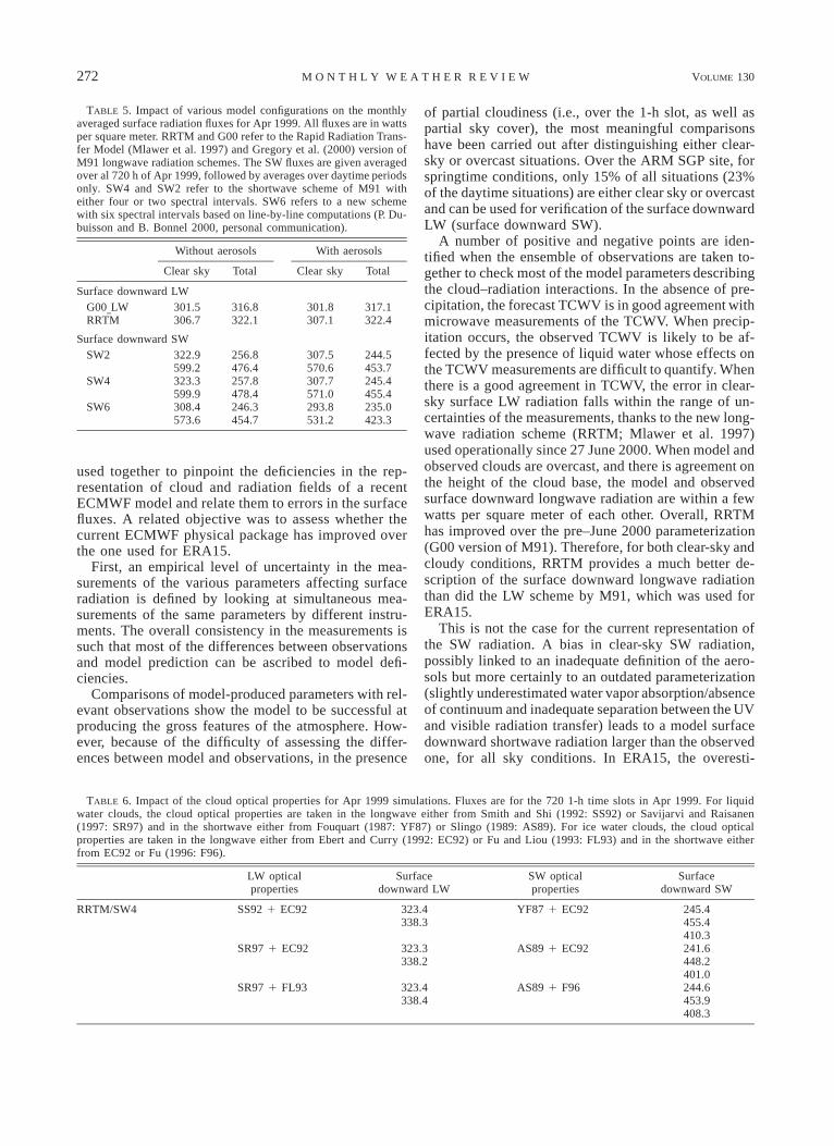
In the operational radiation scheme, the water cloudoptical properties are defined from Smith and Shi (1992)in the LW and Fouquart (1987) in the SW. The effectiveradius for water clouds is specified as 10 mm over land.For ice clouds, optical properties are taken from Ebertand Curry (1992) in both the LW and SW. Table 6compares the surface downward fluxes, for the monthof April, computed with the same radiation schemesincluding different sets of cloud optical properties. Wa-ter cloud optical properties are defined from Savijarviand Raisanen (1997) in the LW and Slingo (1989) inthe SW. Ice cloud optical properties are taken from Fuand Liou (1993) in the LW and Fu (1996) in the SW.The results presented in Table 6 are obtained using thesame profiles of temperature, humidity, cloud fraction,and cloud liquid and ice water to concentrate on theimpact of the cloud optical properties. The impact of thevarious formulations is very small: the change in surfacedownward LW radiation is smaller than 0.2 W m22 whenconcentrating on the cloudy situations. In a similar way,the change in surface downward SW radiation is smallerthan 10 W m22 for the daytime-only cloudy situations.When repeating the calculations with profiles obtainedwith the various formulations for cloud optical propertiesinteractive in the model, the differences are similar orsmaller.

Table 7 presents results obtained with the effectiveradius of water clouds diagnosed from the cloud liquidwater content following Martin et al. (1994) for fourdifferent concentrations of cloud condensation nuclei(300, 600, 900, and 1200 cm23). The impact in the LWis negligible because clouds, when present, are essen-tially black for computing the surface downward LWflux. However, for the surface downward SW flux, a


FIG. 11. The (top) cloud ice water and (bottom) cloud liquid water produced by the ECMWF model over the ARM SGP site. Plottedquantity is the decimal logarithm of the cloud water content (g m23).

larger concentration of cloud condensation nuclei(CCN) for the same condensed water leads to smallerdroplets and more effective scattering of SW radiation.A 10 W m22 decrease in surface downward shortwaveradiation, computed for daytime-only cloudy situations,is seen when CCN concentration is changed from 300to 1200 cm23, a range typical of continental conditions,according to Martin et al. (1994). Thus the major un-

certainty in the modeling of the radiative properties ofwarm clouds is in the specification of the effective radiusvia the number concentration of droplets.

5. Discussion and conclusions

From comparisons with surface radiation measure-ments, Wild et al. (1998a,b) have shown the surface


FIG. 12. (top) The pseudo–radar reflectivity computed from the ECMWF model using the relationships from Frisch et al. (1995) for LWC–Ze and Atlas et al. (1995) for IWC–Ze. (bottom) The radar reflectivity actually measured at the ARM SGP site. The reflectivity is the bestestimate as discussed in Clothiaux et al. (2000). Step is 10 dBZ.

radiation fluxes in the ECMWF Reanalysis of the1979–93 period [now called ERA15; Gibson et al.(1997)] to be in error, with generally too-small down-ward LW radiation and too-high SW downward radi-ation. At the time, ERA15 analyses were carried outwith the original version of the LW scheme of M91

and with SW2, the two-spectral-interval version of theSW scheme of Fouquart and Bonnel (1980). Further-more, these comparisons carried out on monthly meansdid not allow disentanglement of the reasons for sucherrors. In this study, the various measurements carriedout at the Central Facility of the ARM SGP site are


TABLE 5. Impact of various model configurations on the monthlyaveraged surface radiation fluxes for Apr 1999. All fluxes are in wattsper square meter. RRTM and G00 refer to the Rapid Radiation Trans-fer Model (Mlawer et al. 1997) and Gregory et al. (2000) version ofM91 longwave radiation schemes. The SW fluxes are given averagedover al 720 h of Apr 1999, followed by averages over daytime periodsonly. SW4 and SW2 refer to the shortwave scheme of M91 witheither four or two spectral intervals. SW6 refers to a new schemewith six spectral intervals based on line-by-line computations (P. Du-buisson and B. Bonnel 2000, personal communication).

Without aerosols

Clear sky Total

With aerosols

Clear sky Total

Surface downward LWG00 LWRRTM

301.5306.7

316.8322.1

301.8307.1

317.1322.4

Surface downward SWSW2

SW4

SW6

322.9599.2323.3599.9308.4573.6

256.8476.4257.8478.4246.3454.7

307.5570.6307.7571.0293.8531.2

244.5453.7245.4455.4235.0423.3

TABLE 6. Impact of the cloud optical properties for Apr 1999 simulations. Fluxes are for the 720 1-h time slots in Apr 1999. For liquidwater clouds, the cloud optical properties are taken in the longwave either from Smith and Shi (1992: SS92) or Savijarvi and Raisanen(1997: SR97) and in the shortwave either from Fouquart (1987: YF87) or Slingo (1989: AS89). For ice water clouds, the cloud opticalproperties are taken in the longwave either from Ebert and Curry (1992: EC92) or Fu and Liou (1993: FL93) and in the shortwave eitherfrom EC92 or Fu (1996: F96).

LW opticalproperties

Surfacedownward LW

SW opticalproperties

Surfacedownward SW

RRTM/SW4 SS92 1 EC92 323.4338.3

YF87 1 EC92 245.4455.4410.3

SR97 1 EC92 323.3338.2

AS89 1 EC92 241.6448.2401.0

SR97 1 FL93 323.4338.4

AS89 1 F96 244.6453.9408.3

used together to pinpoint the deficiencies in the rep-resentation of cloud and radiation fields of a recentECMWF model and relate them to errors in the surfacefluxes. A related objective was to assess whether thecurrent ECMWF physical package has improved overthe one used for ERA15.

First, an empirical level of uncertainty in the mea-surements of the various parameters affecting surfaceradiation is defined by looking at simultaneous mea-surements of the same parameters by different instru-ments. The overall consistency in the measurements issuch that most of the differences between observationsand model prediction can be ascribed to model defi-ciencies.

Comparisons of model-produced parameters with rel-evant observations show the model to be successful atproducing the gross features of the atmosphere. How-ever, because of the difficulty of assessing the differ-ences between model and observations, in the presence

of partial cloudiness (i.e., over the 1-h slot, as well aspartial sky cover), the most meaningful comparisonshave been carried out after distinguishing either clear-sky or overcast situations. Over the ARM SGP site, forspringtime conditions, only 15% of all situations (23%of the daytime situations) are either clear sky or overcastand can be used for verification of the surface downwardLW (surface downward SW).

A number of positive and negative points are iden-tified when the ensemble of observations are taken to-gether to check most of the model parameters describingthe cloud–radiation interactions. In the absence of pre-cipitation, the forecast TCWV is in good agreement withmicrowave measurements of the TCWV. When precip-itation occurs, the observed TCWV is likely to be af-fected by the presence of liquid water whose effects onthe TCWV measurements are difficult to quantify. Whenthere is a good agreement in TCWV, the error in clear-sky surface LW radiation falls within the range of un-certainties of the measurements, thanks to the new long-wave radiation scheme (RRTM; Mlawer et al. 1997)used operationally since 27 June 2000. When model andobserved clouds are overcast, and there is agreement onthe height of the cloud base, the model and observedsurface downward longwave radiation are within a fewwatts per square meter of each other. Overall, RRTMhas improved over the pre–June 2000 parameterization(G00 version of M91). Therefore, for both clear-sky andcloudy conditions, RRTM provides a much better de-scription of the surface downward longwave radiationthan did the LW scheme by M91, which was used forERA15.

This is not the case for the current representation ofthe SW radiation. A bias in clear-sky SW radiation,possibly linked to an inadequate definition of the aero-sols but more certainly to an outdated parameterization(slightly underestimated water vapor absorption/absenceof continuum and inadequate separation between the UVand visible radiation transfer) leads to a model surfacedownward shortwave radiation larger than the observedone, for all sky conditions. In ERA15, the overesti-


TABLE 7. Impact of the dimension of the water cloud effectiveradius for Apr 1999 simulations. For the surface downward SW ra-diation, the three values correspond to the average over all 720 1-hsimulations in Apr 1999, to the average over the daytime cases only,and to the average over the daytime cases for which the total cloud-iness is larger than 1%.

Dropletconcentration

(cm23)Surface

downward LWSurface

downward SW

RRTM/SW4SS92 1 EC92

300 323.4338.3

242.5450.0403.2

600 323.4338.3

240.0445.3397.1

900 323.4338.3

239.0443.5394.8

1200 323.4338.3

238.6442.8393.9

mation of surface downward SW in clear-sky atmo-spheres was thought to be linked to the two-intervalspectral structure of the SW radiation scheme (M91).The SW4 version of the scheme, operational at the endof 2000, has four spectral intervals and still shows asimilar overestimation. The better spectral descriptionhas only slightly improved the near-infrared absorptionby clouds. A new version of the scheme, including sixspectral intervals, with absorption coefficients derivedfrom line-by-line computations, corrects for a large frac-tion of the overestimation of the surface downward SWin clear-sky conditions. The remaining error might belinked to the effect of subvisible cirrus clouds, a featurecommon above the ARM SGP site, and/or the effect (2W m22) of the thermal offset in the daytime pyranometermeasurements.

Dong et al. (2000) recently studied the seasonal var-iability in the characteristics of the low-level waterclouds above the ARM SGP site, particularly in theeffective radius size and cloud droplet number concen-trations. They showed a factor of 2 increase in clouddroplet number concentrations in winter relative to sum-mer conditions. Independent of the quality of the modelcloud water content, the effective radius of the modelwater cloud droplets, currently specified at 10 mm, islikely to contribute to the underestimation of such avariability in the shortwave radiation fields. The netsurface radiation budget shows a deficient diurnal cycle,with too-large input (by 20–30 W m22) to the surfaceduring daytime and too-large energy loss (by a similaramount) during nighttime. This problem is linked to thedeficiencies discussed above and to the representationof the cloudiness.

Information from the multimode cloud radar was usedfor validating the model cloudiness. As already shownin this and other studies (Mace et al. 1998; Miller et al.1999), the ECMWF cloud scheme is able to represent

the gross features of the cloudiness in terms of presenceand vertical distribution of the cloud layers. However,the cloud water content is a quantity for which therehave been, up to now, very few direct measurementsthat would allow for a detailed model validation. Atentative assessment of the vertical distribution of themodel cloud water content has been carried out in thisstudy. Given the many uncertainties in the relationshipsbetween cloud water content and radar reflectivity, ris-ing mainly from the definition of the particle effectivediameter, we preferred simulating directly the radar re-flectivity to retrieving cloud water from the measure-ments. When using IWC–Ze and LWC–Ze relationshipsfor which the implicit cloud microphysical parametersare equal or similar to the model values, reasonableagreement is found between model-simulated and radar-observed reflectivity, particularly for higher-levelclouds. For liquid water clouds, the model-simulatedreflectivity is usually too small. This might be due partlyto an inaccurate effective radius, given that tests witha diagnosed effective radius or different particle numberconcentrations probably have a large effect on both thecloud reflectivity and the surface downward SW radi-ation underneath such clouds.

Note that, for high clouds, the good visual agreementseen in Fig. 12 is not a proof that the ECMWF modelcloud ice water is realistic, because the equivalent ra-dius assumed for the particles might be different fromreality. This statement is the only one that can be madein the absence of an observational constraint on thisparameter.

After this assessment and other studies that will bereported elsewhere, the ECMWF operational systemwill be modified to include the six-spectral-interval ver-sion of the SW scheme and the diagnosed effective ra-dius for liquid water clouds of Martin et al. (1994).

Acknowledgments. Dr. Clothiaux is gratefully thankedfor providing the radar and micropulse lidar measure-ments used in this study. Thanks are given to RobinPerez for help in acquiring all the other observationaldata and pointing to the relevant documentation. Theseobservational data were obtained from the AtmosphericRadiation Measurement Program sponsored by the U.S.Department of Energy, Office of Science, Office of Bi-ological and Environmental Research, EnvironmentalSciences Division. Drs. Robin Hogan (University ofReading) and Peter Bauer (ECMWF) are thanked fortheir insight on radar reflectivity. At ECMWF, Domi-nique Lucas is thanked for answering numerous queriesabout the HDF and NETCDF packages and Drs. Hol-lingsworth, Miller, Beljaars, and Chevallier are thankedfor their remarks on the manuscript. Drs. Dubuisson andBonnel (LOA, Lille, France) are thanked for providingthe absorption coefficients used within the six-spectral-interval version of the shortwave scheme. I am indebtedto one anonymous reviewer whose extensive commentshelped to clarify the paper.


TABLE A1. Relationship between 35-GHz reflectivity and cloud water content. For Matrosov (1997), the sets of formulas correspond totwo extreme cases (ASTEX, 23 Jun 1992, and the Arizona Program, 3 Mar 1995, respectively) showing a high and low correlationbetween reflectivity and IWC. For Hogan and Illingworth (1999), the sets of formulas correspond to ASTEX and CEPEX cases, respec-tively.

Reference Ice Liquid

Atlas (1954) LWC 5 4.56Ze0.5

Ze 5 0.048LWC2

Sassen (1987) IWC 5 0.037Ze0.7

Ze 5 111.6IWC 1.43

Sauvageot and Omar (1987) LWC 5 5.06Ze0.53

Ze 5 0.047LWC1.83

Liao and Sassen (1994) IWC 5 0.027Ze0.78

Ze 5 102.6IWC 1.28

LWC 5 7.49Ze0.78

Ze 5 0.076LWC1.28

Atlas et al. (1995) IWC 5 0.064Ze0.55

Ze 5 148.0IWC 1.82

Frisch et al. (1995) LWC 5 0.30 rw Ze0.5 No0.5

Ze 5 11.1LWC2/(No rw2)

Matrosov (1997) IWC 5 0.112Ze0.68

Ze 5 25IWC 1.47

IWC 5 0.095Ze0.48

Ze 5 134.7IWC 2.08

Hogan and Illingworth (1999) log10(IWC) 5 0.0619Ze 2 1.078log10(IWC) 5 0.0617Ze 2 0.899

APPENDIX

Reflectivity from the Multimode Cloud Radar andthe Model Water Content

In this study, measurements from the multimodecloud radar are used to evaluate the model cloudinessby following closely the approach used by Beesley etal. (2000) with the Surface Heat Budget of the ArcticOcean (SHEBA) dataset. MMCR is a 34.86-GHz (8.66mm, Ka band) radar. It has been extensively describedin Clothiaux et al. (1999, 2000). Here the argumentsused in the processing of ice and/or liquid water contentfrom the observed radar reflectivities are summarized.

To get the relationship between the radar reflectivityand the cloud water content, I consider the Rayleighapproximation to the Mie scattering theory, that is, thatthe diameter D of the particle must be small in com-parison with the radar wavelength l. From Marshall andGunn (1952), it also is assumed that the radar back-scattering cross section of a small nonspherical particleis equivalent to that of a sphere of the same mass, pro-vided that the particle has the weak dielectric propertiesof a substance such as ice.

It is assumed that the particle size distribution followsa distribution of the form

bN(D) 5 AD exp(2bD),

where D is the diameter; b is the shape parameter (vary-ing between 0 and 3); b 5 1/Do, the inverse of the modediameter of the distribution; and A is related to No/Dob,with No being the number concentration. According toKosarev and Mazin (1991), b 5 0 gives an exponentialfunction that describes large particles with D larger than200 mm, b 5 1 gives a gamma distribution suitable inthe range 20–200 mm, and b 5 2 might apply to smallerparticles with Do around 3–5 mm.

The reflectivity is given by

`

6 (b17)Ze 5 N(D)D dD and Ze 5 A(b 1 6)!/b .E0

The water content is thus related to the distribution by

(b14)WC 5 prA(b 1 3)!/[6b ],

where r is the density. The conventional approach usingZe, the water equivalent radar reflectivity factor, is fol-lowed.

The inference of cloud water content from radar-mea-sured reflectivities is a difficult task inasmuch as therelationship between Ze and LWC or IWC is not unique-ly defined. In the past, numerous relationships have beenproposed that might not be applicable to clouds in morethan one geographical area. The variability of such arelationship is linked to the phase of the cloud particles,their density, and the particle size distribution (Atlas etal. 1995; Matrosov 1997).

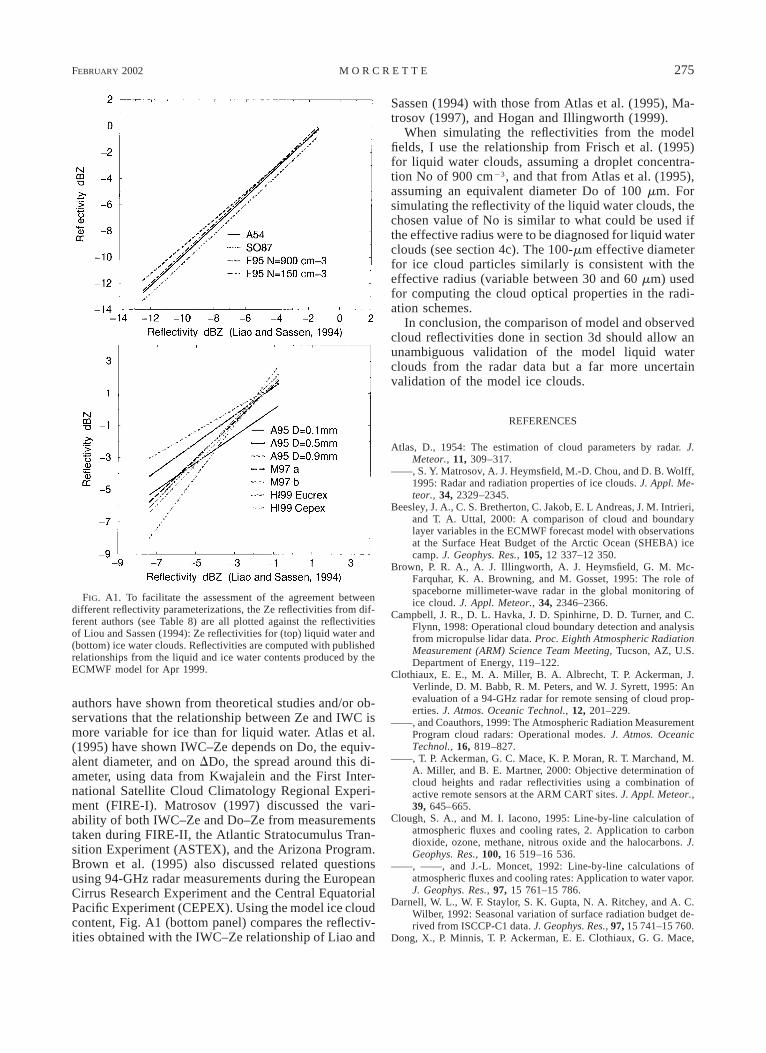
To see what might be possible in terms of modelvalidation, the cloud water profiles produced by theECMWF model have been used with relationships inTable A1, linking the radar reflectivity at 35 GHz withthe cloud liquid or ice water content. For liquid waterclouds, there is a reasonable agreement between rela-tionships proposed by various authors to link Ze toLWC. Figure A1 (top panel) compares the relationshipsby Atlas (1954), Sauvageot and Omar (1987), and Frischet al. (1995) with the one discussed by Liao and Sassen(1994). All the curves have a slope relatively close tounity, and the spread at both ends of the range (corre-sponding to LWC of 2 3 1026 and 3.6 g m23, respec-tively) is smaller than 20 dBZ. Thus one can have con-fidence in inferences drawn for water clouds.

The situation for ice is far less clear, given that various


FIG. A1. To facilitate the assessment of the agreement betweendifferent reflectivity parameterizations, the Ze reflectivities from dif-ferent authors (see Table 8) are all plotted against the reflectivitiesof Liou and Sassen (1994): Ze reflectivities for (top) liquid water and(bottom) ice water clouds. Reflectivities are computed with publishedrelationships from the liquid and ice water contents produced by theECMWF model for Apr 1999.

authors have shown from theoretical studies and/or ob-servations that the relationship between Ze and IWC ismore variable for ice than for liquid water. Atlas et al.(1995) have shown IWC–Ze depends on Do, the equiv-alent diameter, and on DDo, the spread around this di-ameter, using data from Kwajalein and the First Inter-national Satellite Cloud Climatology Regional Experi-ment (FIRE-I). Matrosov (1997) discussed the vari-ability of both IWC–Ze and Do–Ze from measurementstaken during FIRE-II, the Atlantic Stratocumulus Tran-sition Experiment (ASTEX), and the Arizona Program.Brown et al. (1995) also discussed related questionsusing 94-GHz radar measurements during the EuropeanCirrus Research Experiment and the Central EquatorialPacific Experiment (CEPEX). Using the model ice cloudcontent, Fig. A1 (bottom panel) compares the reflectiv-ities obtained with the IWC–Ze relationship of Liao and

Sassen (1994) with those from Atlas et al. (1995), Ma-trosov (1997), and Hogan and Illingworth (1999).

When simulating the reflectivities from the modelfields, I use the relationship from Frisch et al. (1995)for liquid water clouds, assuming a droplet concentra-tion No of 900 cm23, and that from Atlas et al. (1995),assuming an equivalent diameter Do of 100 mm. Forsimulating the reflectivity of the liquid water clouds, thechosen value of No is similar to what could be used ifthe effective radius were to be diagnosed for liquid waterclouds (see section 4c). The 100-mm effective diameterfor ice cloud particles similarly is consistent with theeffective radius (variable between 30 and 60 mm) usedfor computing the cloud optical properties in the radi-ation schemes.

In conclusion, the comparison of model and observedcloud reflectivities done in section 3d should allow anunambiguous validation of the model liquid waterclouds from the radar data but a far more uncertainvalidation of the model ice clouds.

REFERENCES

Atlas, D., 1954: The estimation of cloud parameters by radar. J.Meteor., 11, 309–317.

——, S. Y. Matrosov, A. J. Heymsfield, M.-D. Chou, and D. B. Wolff,1995: Radar and radiation properties of ice clouds. J. Appl. Me-teor., 34, 2329–2345.

Beesley, J. A., C. S. Bretherton, C. Jakob, E. L Andreas, J. M. Intrieri,and T. A. Uttal, 2000: A comparison of cloud and boundarylayer variables in the ECMWF forecast model with observationsat the Surface Heat Budget of the Arctic Ocean (SHEBA) icecamp. J. Geophys. Res., 105, 12 337–12 350.

Brown, P. R. A., A. J. Illingworth, A. J. Heymsfield, G. M. Mc-Farquhar, K. A. Browning, and M. Gosset, 1995: The role ofspaceborne millimeter-wave radar in the global monitoring ofice cloud. J. Appl. Meteor., 34, 2346–2366.

Campbell, J. R., D. L. Havka, J. D. Spinhirne, D. D. Turner, and C.Flynn, 1998: Operational cloud boundary detection and analysisfrom micropulse lidar data. Proc. Eighth Atmospheric RadiationMeasurement (ARM) Science Team Meeting, Tucson, AZ, U.S.Department of Energy, 119–122.

Clothiaux, E. E., M. A. Miller, B. A. Albrecht, T. P. Ackerman, J.Verlinde, D. M. Babb, R. M. Peters, and W. J. Syrett, 1995: Anevaluation of a 94-GHz radar for remote sensing of cloud prop-erties. J. Atmos. Oceanic Technol., 12, 201–229.

——, and Coauthors, 1999: The Atmospheric Radiation MeasurementProgram cloud radars: Operational modes. J. Atmos. OceanicTechnol., 16, 819–827.

——, T. P. Ackerman, G. C. Mace, K. P. Moran, R. T. Marchand, M.A. Miller, and B. E. Martner, 2000: Objective determination ofcloud heights and radar reflectivities using a combination ofactive remote sensors at the ARM CART sites. J. Appl. Meteor.,39, 645–665.

Clough, S. A., and M. I. Iacono, 1995: Line-by-line calculation ofatmospheric fluxes and cooling rates, 2. Application to carbondioxide, ozone, methane, nitrous oxide and the halocarbons. J.Geophys. Res., 100, 16 519–16 536.

——, ——, and J.-L. Moncet, 1992: Line-by-line calculations ofatmospheric fluxes and cooling rates: Application to water vapor.J. Geophys. Res., 97, 15 761–15 786.

Darnell, W. L., W. F. Staylor, S. K. Gupta, N. A. Ritchey, and A. C.Wilber, 1992: Seasonal variation of surface radiation budget de-rived from ISCCP-C1 data. J. Geophys. Res., 97, 15 741–15 760.

Dong, X., P. Minnis, T. P. Ackerman, E. E. Clothiaux, G. G. Mace,


C. N. Long, and J. C. Liljegren, 2000: A 25-month database ofstratus cloud properties generated from ground-based measure-ments at the ARM Southern Great Plains site. J. Geophys. Res.,105, 4529–4538.

Ebert, E. E., and J. A. Curry, 1992: A parameterization of ice opticalproperties for climate models. J. Geophys. Res., 97, 3831–3836.

Fouquart, Y., 1987: Radiative transfer in climate models. Physically-Based Modelling and Simulation of Climate and Climatic Chang-es, Part 1, M. E. Schlesinger, Ed., Kluwer Academic, 223–284.

——, and B. Bonnel, 1980: Computations of solar heating of theearth’s atmosphere: A new parameterization. Beitr. Phys. Atmos.,53, 35–62.

Frisch, A. S., C. W. Fairall, and J. B. Snider, 1995: Measurement ofstratus cloud and drizzle parameters in ASTEX with a Ka-bandDoppler radar and a microwave radiometer. J. Atmos. Sci., 52,2788–2799.

Fu, Q., 1996: An accurate parameterization of the solar radiativeproperties of cirrus clouds for climate studies. J. Climate, 9,2058–2082.

——, and K.-N. Liou, 1993: Parameterization of the radiative prop-erties of cirrus clouds. J. Atmos. Sci., 50, 2008–2025.

Garratt, J. R., 1994: Incoming shortwave fluxes at the surface: Acomparison of GCM results with observations. J. Climate, 7,72–80.

——, and A. J. Prata, 1996: Downwelling longwave fluxes at con-tinental surfaces—a comparison of observations with GCM sim-ulations and implications for the global land-surface radiationbudget. J. Climate, 9, 646–655.

——, ——, L. D. Rotstayn, B. J. McAvaney, and S. Cusack, 1998:The surface radiation budget over oceans and continents. J. Cli-mate, 11, 1951–1968.

Gibson, J. K., P., Kallberg, S. Uppala, A. Nomura, A. Hernandez,and E. Serrano, 1997: The ECMWF Re-Analysis description.ECMWF Re-Analysis Project Report Series, Vol 1, 71 pp.

Gregory, D., J.-J. Morcrette, C. Jakob, A. C. M. Beljaars, and T.Stockdale, 2000: Revision of convection, radiation and cloudschemes in the ECMWF Integrated Forecasting System. Quart.J. Roy. Meteor. Soc., 126, 1685–1710.

Hogan, R. J., and A. J. Illingworth, 1999: The potential of spacebornedual-wavelength radar to make global measurements of cirrusclouds. J. Atmos. Oceanic Technol., 16, 518–531.

Holben, B. N., and Coauthors, 1998: AERONET—A federated in-strument network and data archive for aerosol characterization.Remote Sens. Environ., 66, 1–16.

Holloway, J. L., and S. Manabe, 1971: Simulation of climate by aglobal general circulation model. 1. Hydrologic cycle and heatbalance. Mon. Wea. Rev., 99, 335–370.

Hortal, M., and A. J. Simmons, 1991: Use of reduced Gaussian gridsin spectral models. Mon. Wea. Rev., 119, 1057–1074.

Illari, L., 1987: The ‘‘spin-up’’ problem. ECMWF Tech. Memo. 137,ECMWF, Reading, United Kingdom, 31 pp.

Jakob, C., and S. A. Klein, 2000: A parameterization of the effectsof cloud and precipitation overlap for use in general circulationmodels. Quart. J. Roy. Meteor. Soc., 126C, 2525–2544.

Kosarev, A. L., and I. P. Mazin, 1991: An empirical model of thephysical structure of upper-level clouds. Atmos. Res., 26, 213–228.

Laszlo, I., and R. T. Pinker, 1993: Shortwave cloud-radiative forcingat the top of the atmosphere, at the surface and of the atmosphericcolumn as determined from ISCCP C1 data. J. Geophys. Res.,98, 2703–2718.

Li, Z., and H. G. Leighton, 1993: Global climatologies of solar ra-diation budgets at the surface and in the atmosphere from 5 yearsof ERBE data. J. Geophys. Res., 98, 4919–4930.

Liao, L., and K. Sassen, 1994: Investigation of relationships betweenKa-band radar reflectivity and ice and liquid water contents.Atmos. Res., 34, 231–248.

Mace, G. G., and K. Sassen, 2000: A constrained algorithm for re-trieval of stratocumulus cloud properties using solar radiation,

microwave radiometer, and millimeter cloud radar data. J. Geo-phys. Res., 105, 29 099–29 108.

——, C. Jakob, and K. P. Moran, 1998: Validation of hydrometeoroccurrence predicted by the ECMWF model using millimeterwave radar data. Geophys. Res. Lett., 25, 1645–1648.

Mahfouf, J.-F., and F. Rabier, 2000: The ECMWF operational imple-mentation of four dimensional variational assimilation: Part II:Experimental results with improved physics. Quart. J. Roy. Me-teor. Soc., 126A, 1171–1190.

Marshall, J. S., and K. L. S. Gunn, 1952: Measurement of snowparameters by radar. J. Meteor., 9, 322–327.

Martin, G. M., D. W. Johnson, and A. Spice, 1994: The measurementand parameterization of effective radius of droplets in warmstratocumulus. J. Atmos. Sci., 51, 1823–1842.

Matrosov, S. Y., 1997: Variability of microphysical parameters inhigh-altitude ice clouds: Results of the remote sensing methods.J. Appl. Meteor., 36, 633–648.

Matveev, Yu. L., 1984: Cloud Dynamics. D. Reidel, 340 pp.Miller, S. D., G. L. Stephens, and A. C. M. Beljaars, 1999: A vali-

dation survey of the ECMWF prognostic cloud scheme usingLITE. Geophys. Res. Lett., 26, 1417–1420.

Mlawer, E. J., S. J. Taubman, P. D. Brown, M. J. Iacono, and S. A.Clough, 1997: Radiative transfer for inhomogeneous atmo-spheres: RRTM, a validated correlated-k model for the long-wave. J. Geophys. Res., 102, 16 663–16 682.

Morcrette, J.-J., 1991: Radiation and cloud radiative properties in theECMWF operational weather forecast model. J. Geophys. Res.,96, 9121–9132.

——, 1993: Revision of the clear-sky and cloud radiative propertiesin the ECMWF model. ECMWF Newsletter, Vol. 61, 3–14.

——, 2000: On the effects of the temporal and spatial sampling ofradiation fields on the ECMWF forecasts and analyses. Mon.Wea. Rev., 128, 876–887.

——, S. A. Clough, E. J. Mlawer, and M. J. Iacono, 1998: Impactof a validated radiative transfer scheme, RRTM, on the ECMWFmodel climate and 10-day forecasts. ECMWF Tech. Memo. 252,ECMWF, Reading, United Kingdom, 47 pp.

Ohmura, A., and H. Gilgen, 1993: Re-evaluation of the global energybalance. Interactions between Global Climate Subsystems, Geo-phys. Monogr., Vol. 75, No. 15, Amer. Geophys. Union, 93–110.

Rabier, F., J.-N. Thepaut, and P. Courtier, 1998: Extended assimilationand forecasts experiments with a four dimensional variationalassimilation system. Quart. J. Roy. Meteor. Soc., 124, 1861–1887.

Rothman, L. S., and Coauthors, 1987: The HITRAN database: 1986edition. Appl. Opt., 26, 4058–4097.

——, and Coauthors, 1992: The HITRAN database: Editions of 1991and 1992. J. Quant. Spectrosc. Radiat. Transfer, 48, 469–507.

——, and Coauthors, 1996: HITRAN molecular database: Edition’96. J. Quant. Spectrosc. Radiat. Transfer, 60, 665–710.

Sassen, K., 1987: Ice cloud content from radar reflectivity. J. ClimateAppl. Meteor., 26, 1050–1053.

Sauvageot, H., and J. Omar, 1987: Radar reflectivity of cumulusclouds. J. Atmos. Oceanic Technol., 4, 264–272.

Savijarvi, H., and P. Raisanen, 1997: Long-wave optical propertiesof water clouds and rain. Tellus, 50A, 1–11.

Slingo, A., 1989: A GCM parameterization for the shortwave radi-ative properties of water clouds. J. Atmos. Sci., 46, 1419–1427.

Smith, E. A., and L. Shi, 1992: Surface forcing of the infrared coolingprofile over the Tibetan plateau. Part I: Influence of relativelongwave radiative heating at high altitude. J. Atmos. Sci., 49,805–822.

Stokes, G. M., and S. E. Schwartz, 1994: The Atmospheric RadiationMeasurement (ARM) Program: Programmatic background anddesign of the cloud and radiation test bed. Bull. Amer. Meteor.Soc., 75, 1201–1221.

Tanre, D., J.-F. Geleyn, and J. Slingo, 1984: First results of the in-troduction of an advanced aerosol-radiation interaction in theECMWF low resolution global model. Aerosols and Their Cli-


matic Effects, H. E. Gerber and A. Deepak, Eds., A. DeepakPublishing, 133–177.

Temperton, C., M. Hortal, and A. Simmons, 2001: A two-time-levelsemi-Lagrangian global spectral model. Quart. J. Roy. Meteor.Soc., 127A, 111–127.

Tiedtke, M., 1993: Representation of clouds in large-scale modelsMon. Wea. Rev., 121, 3040–3061.

——, 1996: An extension of cloud–radiation parameterization in theECMWF model: The representation of subgrid-scale variationsof optical depth. Mon. Wea. Rev., 124, 745–750.

van den Hurk, B. J. J. M., P. Viterbo, A. C. M. Beljaars, and A. K.Betts, 2000: Offline validation of the ERA40 surface scheme.ECMWF Tech. Memo. 295, ECMWF, Reading, United Kingdom,42 pp.

Vonder Haar, T. H., 1969: Variations of the earth’s radiation budget.Ph.D. thesis, University of Wisconsin—Madison, 116 pp.

Westwater, E. R., Remote sensing of column integrated water vapor

by microwave radiometers and GPS during the 1997 water vaporintensive observation period. Proc. Eighth Atmospheric Radia-tion Measurement (ARM) Science Team Meeting, Tucson, AZ,U.S. Department of Energy, 799–803.

Wild, M., A. Ohmura, H. Gilgen, and E. Roeckner, 1995: Validationof general circulation model radiative fluxes using surface ob-servations. J. Climate, 8, 1309–1324.

——, ——, ——, and J.-J. Morcrette, 1998a: The distribution ofsolar energy at the earth’s surface as calculated in the ECMWFRe-Analysis. Geophys. Res. Lett., 25, 4373–4376.

——, ——, ——, E. Roeckner, M. Giorgetta, and J.-J. Morcrette,1998b: The disposition of radiative energy in the global climatesystem: GCM-calculated vs. observations estimates. ClimateDyn., 14, 853–869.

——, ——, ——, J.-J. Morcrette, and A. Slingo, 2001: Evaluationof the downward longwave radiation in general circulation mod-els. J. Climate, 14, 3227–3239.

Assessment of the ECMWF Model Cloudiness and Surface Radiation Fields at the ARM SGP Site (2002)

Documents

Transcript of Assessment of the ECMWF Model Cloudiness and Surface Radiation Fields at the ARM SGP Site (2002)