Linearized radiation and cloud schemes in the ECMWF model: Development and evaluation (2002)

Q. J. R. Meteorol. Soc. (2002), 128, pp. 1505–1527

Linearized radiation and cloud schemes in the ECMWF model:Development and evaluation

By MARTA JANISKOVA∗, JEAN-FRANCOIS MAHFOUF, JEAN-JACQUES MORCRETTEand FREDERIC CHEVALLIER

European Centre for Medium-Range Weather Forecasts, UK

(Received 20 September 2001; revised 29 January 2002)

SUMMARY

A proper consideration of cloud–radiation interactions in linearized models is required for variationalassimilation of cloud properties. Therefore, both a linearized cloud scheme and a linearized radiation schemehave been developed for the European Centre for Medium-Range Weather Forecasts (ECMWF) data assimilationsystem. The tangent-linear and adjoint versions of the ECMWF short-wave radiation scheme are prepared withouta priori modifications. The complexity of the radiation scheme for the long-wave part of the spectrum makesaccurate computations expensive. To reduce its computational cost, a combination of artificial neural networksand Jacobian matrices is defined for the linearized long-wave radiation scheme. The linearized cloud scheme isdiagnostic and has been adapted for this study. The accuracy of the linearization of both radiation and diagnosticcloud schemes is examined. The inclusion of a more sophisticated radiation scheme within the existing linearizedparametrizations improves the accuracy of the tangent-linear approximation. However, the impact of the linearizeddiagnostic cloud scheme is small, suggesting that the linearized model will require further developments of cloudparametrization.

The adjoint technique is used to investigate the sensitivity of the radiation schemes to changes in temperature,humidity and cloud properties. This study shows which variables can be adjusted when certain observations of thesurface and/or of the top-of-atmosphere radiation fluxes are used in data assimilation. It also indicates the verticalextent of the influence of such observations.

KEYWORDS: Cloud–radiation processes Linearization Sensitivity

1. INTRODUCTION

A large part of forecasting deficiencies is connected with the imperfect assimilationof available observational data in the numerical prediction process. In recent years,four-dimensional variational (4D-Var) data assimilation has become a powerful toolin transferring information from the irregularly distributed observations into initialconditions for a numerical forecast model. 4D-Var minimizes the distance between amodel trajectory and observations spread over a given time interval. The minimizationalgorithm used in 4D-Var employs the adjoint equations of the model to computethe gradient of the cost function with respect to the model state at the beginning ofthe assimilation period. Such an assimilation system was first tested using adiabaticmodels. Rabier and Courtier (1992) and Rabier et al. (1996) have shown that anadiabatic model used in sensitivity studies was able to represent phenomena linkedto baroclinic instability to a reasonable accuracy. However, physical processes play asignificant role in various large-scale and mesoscale phenomena. Neglecting physicalprocesses in the data assimilation systems leads to the so-called spin-up problem dueto an imbalance between the model equations and the initial state. The misfit betweenmodel solution and data can remain large due to the imperfect adiabatic model. Manysatellite observations, such as radiances, rainfall measurements and cloud properties,cannot be directly assimilated into such models; hence it is important that physicalprocesses should be taken into account in the assimilating model. Some studies havebeen undertaken to include physical parametrizations in the adjoint models (Zou et al.

∗ Corresponding author: European Centre for Medium-Range Weather Forecasts, Shinfield Park, Reading,Berkshire RG2 9AX, UK. e-mail: [email protected]© Royal Meteorological Society, 2002.

1505

1506 M. JANISKOVA et al.

1993; Zupanski and Mesinger 1995; Tsuyuki 1996; Zou 1997; Errico and Reader 1999;Janiskova et al. 1999; Mahfouf 1999) with encouraging results.

4D-Var assimilation systems were implemented operationally in November 1997 atthe European Centre for Medium-Range Weather Forecasts (ECMWF) (Klinker et al.2000; Mahfouf and Rabier 2000; Rabier et al. 2000) and in June 2000 at Meteo-France.As the inclusion of physics in the adjoint model improves the performance of 4D-Var,both operational assimilation systems use adjoint models with a set of simplifiedphysical parametrizations developed by Mahfouf (1999) (for the ECMWF model)and Janiskova et al. (1999) (for the Meteo-France forecasting system). Even thoughthe adjoint of various physical parametrization schemes is included in the ECMWFassimilating model, some of them are quite simplified. For radiation, a very simplifiedlinearized long-wave code is used, where no dependency of radiation on cloudiness istaken into account and the short-wave radiation processes are not considered. However,both solar and thermal radiation fluxes are affected by condensed water (in the form ofcloud droplets and ice crystals) as well as by the water-vapour absorption bands. Cloudsplay an important role in the water and energy budgets of the Earth’s atmosphere andtherefore the use of data in cloudy conditions is an important issue for numerical weatherprediction.

Most operational data assimilation systems do not use observations on cloudsavailable from the surface network and satellites. The main reason lies in the difficultyof accurately describing the cloud processes in atmospheric models. However, recentimprovements in the representation of clouds (such as the development of prognosticcloud schemes) and flexible data analysis systems (such as three-dimensional variationaland 4D-Var) make preliminary investigations towards the use of observations in cloudysituations possible. The inclusion of cloud observations in data assimilation should leadto an improved initial state of the model prognostic variables, which could in turnimprove the quality of the forecasts including parameters such as 2-metre temperature,cloudiness and precipitation.

The ECMWF operational 4D-Var assimilation system can assimilate new typesof observations when a proper observation operator exists. The observation operatorsproviding the model counterpart of cloud observations are the linearized versions ofboth a radiative-transfer model and a cloud scheme, which need to be developed for usein variational data assimilation.

Radiative-transfer models in clear sky do not describe strong nonlinear processes(even though some saturation effects can take place in water-vapour absorption bands).Thus, linearized radiation codes have been used successfully for variational assimilationof clear-sky radiances in numerical weather-prediction models (for example Eyre 1995).

The linearization of physical parametrization schemes describing cloud processesand cloud–radiation interactions is not straightforward since the on/off nature of cloudscan make the tangent-linear approximation questionable. Zou and Navon (1996) devel-oped the linearized version of a solar radiative-transfer code where the cloud fractionalamount was taken as a constant input parameter. The Jacobian approach was applied byChou and Neelin (1996) to formulate a linear scheme for long-wave radiative fluxes. Forlinearized cloud fractions, they defined simple cloud-cover types which have a fixed ver-tical structure and which never overlap in the vertical. Janiskova et al. (1999) developeda simplified linearized radiation scheme where the coefficients for short-wave radiation(representing the properties of absorption and multiple scattering) and for long-waveradiation (a matrix of coefficients depending on emissivity and transmission) are storedfrom a one-time-step integration of the full nonlinear scheme and recomputed as a func-tion of cloudiness in the linearized physical parametrization. They reported results on

LINEARIZED RADIATION AND CLOUD SCHEMES 1507

the linearization of a simple diagnostic cloud scheme used with the linearized radiationscheme in a global atmospheric model. Due to the presence of thresholds in the cloudscheme, considerable noise in the solution was observed. Therefore, the perturbations incloud cover were neglected in that study. More encouraging results were obtained at asmaller scale (Verlinde and Cotton 1993; Park and Droegemeier 1997) where linearizedversions of cloud-resolving models were developed with some success for radar retrievalapplications. Chevallier et al. (2001a) showed some capability of a fast infrared andmicrowave radiation model and its linearized version for one-dimensional variational(1D-Var) analyses of cloud-affected ATOVS∗ observations.

Once the linearized versions (tangent-linear and adjoint) of physical parametrizationschemes are developed, they can be used for purposes other than just data assimilation.The model’s adjoint is a powerful tool which enables the estimation of the sensitivityof a given output quantity to all the input variables of a parametrization scheme. Usingthe adjoint technique for the radiation scheme provides the sensitivity of the radiationfluxes to changes in temperature, humidity and cloud properties. Compared with thestandard approaches for evaluation of physical parametrization schemes (sensitivity ofall the outputs to a given input quantity), the adjoint is a complementary approach forsensitivity studies. It can also give indications related to the importance and efficiencyof particular types of observations for data assimilation applications.

In this paper, the development of comprehensive linearized radiation and cloudschemes is presented in the framework of the ECMWF model. In section 2, a briefdescription of the short-wave and long-wave radiation schemes is given with emphasison the incorporation of the effects of clouds on the radiation fluxes. The linearizeddiagnostic cloud scheme is also described there. The tangent-linear approximation isevaluated for cloud–radiation processes in section 3. The adjoint technique is used toinvestigate the sensitivity of radiative fluxes to changes in temperature, humidity andcloud properties. The corresponding methodology and results are described in section 4.Summary and discussions are presented in section 5.

2. DESCRIPTION OF THE LINEARIZED RADIATION AND CLOUD SCHEMES

The linearized radiation code used in the current ECMWF operational 4D-Varaccounts only for the clear-sky long-wave radiation transfer via a constant emissivityformulation (Mahfouf 1999), for which the effective emissivities are stored from thefull nonlinear radiation scheme. As first identified by Thuburn (1994) and explainedalso by Mahfouf (1999), this method can lead to an exponential growth of temperatureincrements when the vertical temperature gradient is negative, which is the case in thestratosphere. Therefore, the linearized long-wave scheme is restricted to the troposphereonly. In the direct model, due to computational costs, the full radiation calculations arepresently done every hour during the first 12 hours of the forecasts, then every 3 hours.Moreover, they are carried out on a reduced horizontal grid (Morcrette 2000).

In order to assimilate cloud observations, the radiative-transfer model must obvi-ously include cloud–radiation interactions. This has led to the development of a lin-earized cloud scheme and of a more sophisticated radiation scheme describing long-wave and short-wave, clear-sky and cloudy radiation transfer. The new linearized radia-tion scheme must also be computationally efficient to be called at each time step and atthe full spatial resolution for an improved description of the cloud–radiation interactionsduring the assimilation period.

∗ Advanced Tiros Operational Vertical Sounder.


(a) The short-wave radiation schemeThe short-wave radiation scheme, originally developed by Fouquart and Bonnel

(1980), is used in the ECMWF model (Morcrette 1989, 1991). The photon-path-distribution method is used to separate the parametrization of the scattering processesfrom that of molecular absorption. Upward F ↑

sw and downward F ↓sw fluxes at a given

level j are obtained from the reflectance and transmittance of the atmospheric layers as:

F ↓sw(j)= F0

N∏k=j

Tbot(k) (1)

F ↑sw(j)= F ↓

sw(j)Rtop(j − 1). (2)

Computations of the transmittance at the bottom of a layer Tbot start at the top ofthe atmosphere and work downward. Those of the reflectance at the top of the samelayer Rtop start at the surface and work upward. In the presence of cloud in the layer,the final fluxes are computed as a weighted average of the fluxes in the clear sky and inthe cloudy fractions of the column as:

Rtop = CcloudRcloud + (1 − Ccloud)Rclear (3)Tbot = CcloudTcloud + (1 − Ccloud)Tclear. (4)

In the previous equations, Ccloud is the cloud fractional coverage of the layer withinthe cloudy fraction of the column (depending on cloud overlap assumptions).

This nonlinear scheme is reasonably fast for application in 4D-Var and has, there-fore, been linearized without a priori modifications.

(b) The long-wave radiation schemeThe long-wave radiation scheme, operational in the ECMWF forecast model until

June 2000, is a band-emissivity type scheme (Morcrette 1989). The long-wave spectrumfrom 0 to 2820 cm−1 is divided into six spectral regions. The transmission functionsfor water vapour and carbon dioxide over those spectral intervals are fitted using Padeapproximations on narrow-band transmissions obtained with statistical band models(Morcrette et al. 1986). Integration of the radiation-transfer equation over wave numberswithin the particular spectral regions gives the upward and downward fluxes. Theincorporation of the effects of clouds on the long-wave fluxes follows the treatmentdiscussed by Washington and Williamson (1977). The fluxes for the actual atmosphereare derived from a linear combination of the fluxes calculated for a clear-sky atmosphereand those obtained assuming a unique overcast cloud of emissivity unity.

The complexity of the radiation scheme for the long-wave part of the spectrummakes accurate computations expensive. In the variational assimilation framework,simplifications were made to reduce its computational cost. A combination of artificialneural networks and mean Jacobians was defined for the linearized long-wave radiation.Such choice is based on the following findings:

• A neural network version (called NeuroFlux) of the ECMWF long-wave radiative-transfer model is significantly faster (seven times) than the operational long-wave radi-ation code with a comparable accuracy. A detailed description of NeuroFlux can befound in Chevallier et al. (1998, 2000).

• Chevallier and Mahfouf (2001) showed that the variability of the clear-skyJacobians does not play an essential role when computing total sky (i.e. includingcloudiness) fluxes and, therefore, pre-computed Jacobians averaged globally can beused.


A description of the linearized long-wave radiation scheme using the two ingredientsmentioned above follows.

The long-wave radiative fluxes depend upon temperature, water vapour, cloud coverand liquid- and ice-water contents. The design of the scheme allows the separationof the contribution of temperature and water vapour from that of cloud parameters.More precisely, the upward and downward long-wave fluxes at a certain height z i areexpressed as:

F(zi)=∑k

ak(zi)Fk(zi) (5)

where the coefficients ak are a function of the cloudiness matrices CC i,k computedusing some overlap assumption defined more precisely in section 2(e). Differentiatingthe above equation, a flux perturbation is computed as:

dF(zi)=∑k

{ak(zi)︸︷︷︸

NL model

dFk(zi)︸︷︷︸Jacobian matrices

+ Fk(zi)︸︷︷︸NeuroFlux

dak(zi)︸︷︷︸TL model

}. (6)

In the proposed approach, the coefficients ak are computed using the nonlinear (NL)model (code computing cloud optical properties). Due to the weak nonlinearities in thevariations of the radiative fluxes Fk with respect to temperature and water vapour, thetangent-linear approximation can be used to compute perturbations of radiation fluxesdFk from pre-computed mean Jacobian matrices. Perturbations of radiative fluxes withrespect to cloud parameters dak(zi) are computed using a tangent-linear (TL) scheme.The trajectory of radiative fluxes required in the tangent-linear and adjoint computationsare efficiently estimated from NeuroFlux in order to avoid significant extra memorystorage or costly re-computations.

(c) Cloud parametrization schemeThe ECMWF diagnostic cloud scheme (Slingo 1987), used before the implemen-

tation of the current operational prognostic scheme (Tiedtke 1993), was linearized to beused with the linearized radiation scheme.

The diagnostic cloud scheme allows for four cloud types: convective cloud andthree types of layer clouds (high, middle and low level). The convective clouds (C conv)are parametrized using the scale-averaged precipitation rate (P ) from the model convec-tion scheme. They can fill any number of model layers and their depth is determined bythe convection scheme. The stratiform clouds (Cstrat) are determined from a function ofthe layer relative humidity (RHe) after adjustment for the presence of convective clouds,RHe = RH − Cconv, as:

Cstrat = f (RHe)={

max

(RHe − b

1 − b, 0

)}2

(7)

where b is equal to 0.8 for high- and middle-level clouds and to 0.7 for low-level clouds.The middle-level clouds and low-level clouds associated with the extratropical frontsare then scaled with vertical velocity in the case of upward motion. There are no suchclouds in subsidence areas.

Liquid water llwc and ice water liwc are proportional to the specific humidity atsaturation qsat. They are defined as

llwc = αllc (8)liwc = (1 − α)llc (9)


where α is the fraction of condensate held as liquid water and l lc = 0.05Ccloudqsat withCcloud being cloud cover.

The linearized diagnostic cloud scheme was further simplified by accounting forpart of the dependencies only. The current linearized convection scheme does notprovide perturbations of precipitation. This leads to a zero perturbation of convectivecloudiness since it is determined from the convective precipitation rate. A modificationof the linearized cloud scheme was also necessary in order to avoid the thresholdproblem in the parametrization of the layer clouds computed as a function of relativehumidity RHe (Eq. (7)). Although this threshold does not lead to any occurrence ofspuriously growing unstable perturbations (Janiskova et al. 2000), it can degrade results,and it was therefore decided to set the derivative of the function of relative humidity tozero. This also means that the high-level cloud cover is then constant for a given timestep. Middle-level and low-level clouds are only modified by vertical velocity. Liquidwater and ice water can, however, be modified by temperature perturbations.

(d) Cloud optical propertiesCloud–radiation interactions depend not only on the cloud fraction or cloud volume,

but also on cloud optical properties. In the case of short-wave radiation, the cloudradiative properties depend on three different parameters: the optical thickness δc, theasymmetry factor gc and the single scattering albedo ωc. These parameters are derivedfrom Fouquart (1987) for water clouds, and Ebert and Curry (1992) for ice clouds. Theyare functions of cloud condensate and a specified effective radius.

Cloud long-wave optical properties are represented by the emissivity εcld related tothe condensed-water amount, and by the condensed-water mass absorption coefficientkabs obtained following Smith and Shi (1992) for water clouds and Ebert and Curry(1992) for ice clouds.

(e) Cloud overlap assumptionsCloud overlap assumptions must be made in atmospheric models in order to

organize the cloud distribution used for radiation and precipitation/evaporation com-putations. A cloud overlap assumption of some sort is necessary to account for the factthat clouds often do not fill the whole grid box. Most atmospheric models use random(RAN), maximum-random (MRN) or maximum (MAX) overlap assumptions in theradiation scheme. The definition of cloud overlap assumptions is given from the point ofview of cloudinessCCi,j encountered between any levels i and j in the atmosphere. LetCk be the cloud fraction of the layer k located between levels k and k + 1. The maximumoverlap assumption gives:

CCi,j = max(Ci, Ci+1, . . . , Cj−1). (10)

The random overlap assumption gives:

CCi,j = 1 −j−1∏k=i(1 − Ck). (11)

The maximum-random overlap assumption gives:

CCi,j = 1 − (1 − Ci)

j−1∏k=i+1

(1 − max(Ck, Ck−1)

1 − Ck−1

). (12)


The maximum-random overlap assumption (originally introduced in Geleyn and Holl-ingsworth 1979) is used operationally in the ECMWF model (Morcrette and Jakob2000). Adjacent layers containing cloud are combined by using maximum overlapto form a contiguous cloud and discrete layers separated by clear sky are combinedrandomly.

3. VALIDATION OF THE LINEARIZED MODEL INCLUDING CLOUD–RADIATION PROCESSES

The classical verification of the correctness of the tangent-linear model is donethrough the Taylor formula:

limλ→0

M(x + λδx)− M(x)M(λδx)

= 1 (13)

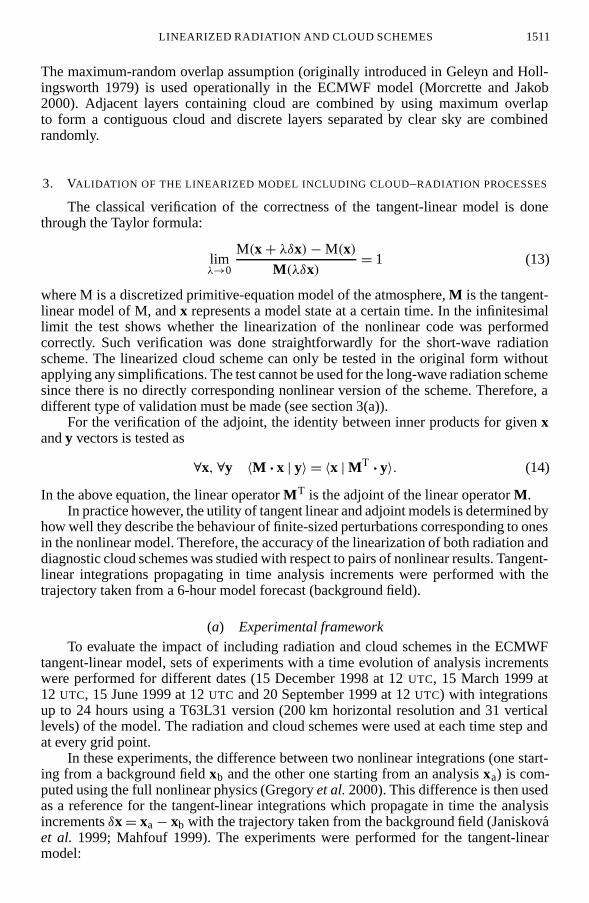
where M is a discretized primitive-equation model of the atmosphere, M is the tangent-linear model of M, and x represents a model state at a certain time. In the infinitesimallimit the test shows whether the linearization of the nonlinear code was performedcorrectly. Such verification was done straightforwardly for the short-wave radiationscheme. The linearized cloud scheme can only be tested in the original form withoutapplying any simplifications. The test cannot be used for the long-wave radiation schemesince there is no directly corresponding nonlinear version of the scheme. Therefore, adifferent type of validation must be made (see section 3(a)).

For the verification of the adjoint, the identity between inner products for given xand y vectors is tested as

∀x, ∀y 〈M · x | y〉 = 〈x | MT · y〉. (14)

In the above equation, the linear operator MT is the adjoint of the linear operator M.In practice however, the utility of tangent linear and adjoint models is determined by

how well they describe the behaviour of finite-sized perturbations corresponding to onesin the nonlinear model. Therefore, the accuracy of the linearization of both radiation anddiagnostic cloud schemes was studied with respect to pairs of nonlinear results. Tangent-linear integrations propagating in time analysis increments were performed with thetrajectory taken from a 6-hour model forecast (background field).

(a) Experimental frameworkTo evaluate the impact of including radiation and cloud schemes in the ECMWF

tangent-linear model, sets of experiments with a time evolution of analysis incrementswere performed for different dates (15 December 1998 at 12 UTC, 15 March 1999 at12 UTC, 15 June 1999 at 12 UTC and 20 September 1999 at 12 UTC) with integrationsup to 24 hours using a T63L31 version (200 km horizontal resolution and 31 verticallevels) of the model. The radiation and cloud schemes were used at each time step andat every grid point.

In these experiments, the difference between two nonlinear integrations (one start-ing from a background field xb and the other one starting from an analysis xa) is com-puted using the full nonlinear physics (Gregory et al. 2000). This difference is then usedas a reference for the tangent-linear integrations which propagate in time the analysisincrements δx = xa − xb with the trajectory taken from the background field (Janiskovaet al. 1999; Mahfouf 1999). The experiments were performed for the tangent-linearmodel:


• without radiation,• with the current operational radiation scheme (hereafter referred as OPER radia-

tion),• with the new short-wave and long-wave radiation schemes described in the previ-

ous section (new radiation) run without/with the cloud scheme (clear sky/cloudiness).

This set of experiments enables the evaluation of improvements coming from theinclusion of a radiation scheme in the existing set of linearized physics, whether the newradiation scheme is better than the OPER scheme, and what improvement is brought bythe cloud scheme used with the new radiation scheme.

For a quantitative evaluation of the impact of the cloud and radiation schemes, theirrelative importance is evaluated using mean absolute errors between tangent-linear andnonlinear integrations as

ε = |{M(xa)− M(xb)} − M(xa − xb)| (15)

where M is the forecast model starting from different initial conditions:

xa—from the analysis,xb—from the background,

M is the tangent-linear model starting from the initial conditions(xa − xb),

(. . . ) represents the mean over a particular domain.

As a reference for the comparisons, an absolute mean error for the tangent-linearmodel without any radiation or with the OPER radiation εref is taken. εi represents theabsolute mean error for the tangent-linear model including radiation and cloud schemeswith respect to pairs of nonlinear integrations with full physics. Then an improvementcoming from including more physics in the tangent-linear model should correspond toεi being less than εref.

The impact of including the new radiation and cloudiness schemes was evaluatedby studying the time evolution of analysis increments at different model levels and usingthe zonal-mean average of the mean absolute errors. Global zonal-mean errors as wellas zonal-mean errors for 20◦N–90◦N (North20), 20◦S–90◦S (South20) and 20◦N–20◦S(Tropics) were evaluated separately.

The radiation directly influences the temperature field and as a consequence of thesetemperature changes the impact of the radiation on other quantities can be observed.Hence results are mostly presented for temperature perturbations although, during thevalidation, the results from other fields were also compared.

(b) Results of the validation experimentsThe experiments were performed for different dates (as listed in section 3(a)).

Results from only two of the situations are presented here.Figure 1 shows comparisons of the TL integrations where the trajectory is computed

with the diagnostic cloud scheme (as was used operationally in the ECMWF 4D-Var).The TL models using the physical package described in Mahfouf (1999) with either theOPER radiation scheme or with the new radiation and cloud schemes are compared withthe TL model without any radiation (reference TL model). Negative values (positivevalues) are associated with an improvement (deterioration) of the TL model with respectto the reference one since they correspond to a reduction (increase) of the error ε referredto in Eq. (15). It can be seen that the OPER radiation scheme (Fig. 1(a)) only gives a


a)

b)

mod

el le

vels

m

odel

leve

ls

L30 ~ 980 hPa L25 ~ 810 hPa L20 ~ 580 hPa L15 ~ 375 hPa L10 ~ 200 hPa L5 ~ 90 hPa

Figure 1. Influence of the different tangent-linear (TL) radiation schemes on the evolution of temperatureincrements with the trajectory computed using the diagnostic cloud scheme. Results are presented as the errordifferences (in terms of fit to the nonlinear model with full physics) between the TL model including operationallinearized physics (OPER radiation) and the TL model without any radiation (a). (b) Presents the same, but forthe TL model containing the new radiation scheme with the simplified diagnostic cloud scheme. (24-hour forecast

for the situation of 15 March 1999, 12 UTC, units: K).

slight global improvement of 0.31%. Negative impacts appear in the upper troposphere.This problem comes from the use of the constant-emissivity approach, which is notappropriate in the stratosphere. The new radiation and cloud schemes (Fig. 1(b)) give aglobal improvement of 4.71%. There are only a few small negative impacts.

The vertical profiles for the global-mean values of εi − εref and the global-meanabsolute errors εref are presented in Fig. 2 for a 24-hour integration. The results fortemperature, specific humidity and u wind component are on the left, middle and right


−0.04 −0.03 −0.02 −0.01 0.00 0.01

5

10

15

20

25

30

mod

el le

vels

Mean of error differences for temperature

T

a

−0.03 −0.02 −0.01 0.00 0.01

5

10

15

20

25

30

Mean of error differences for specific humidity

q

b

−0.08 −0.06 −0.04 −0.02 0.00

5

10

15

20

25

30

Mean of error differences for u−wind

u

c

0.0 0.1 0.2 0.3 0.4

5

10

15

20

25

30

mod

el le

vels

Mean absolute error for temperature

T

d

0.0 0.1 0.2 0.3

5

10

15

20

25

30

Mean absolute error for specific humidity

q

e

0.0 0.2 0.4 0.6 0.8 1.0

5

10

15

20

25

30

Mean absolute error for u−wind

u

f

Figure 2. Vertical profiles of the global-mean values of error differences (top panels) and the global-meanabsolute errors (bottom panels) for temperature (units: K), specific humidity (units: g kg−1) and uwind component(units: m s−1) from a 24-hour integration. The results are presented for the currently used radiation scheme (dashedline) as well as for the new radiation scheme with cloudiness (solid line) and for clear sky (dot-dashed line). Initial

date of the integration: 15 March 1999, 12 UTC. Model levels are as shown in Fig. 1.

panels, respectively. The comparisons are displayed for the OPER (simplified) long-wave radiation scheme as well as for the new radiation (long wave and short wave) withthe simplified cloud scheme and for clear sky.

By comparing the impact of the schemes on temperature, Fig. 2(a) shows thatincluding the new radiation in the linearized physics improves quantitatively the fit ofthe tangent-linear model to the nonlinear one through the whole vertical profile. Addingthe cloud scheme to the radiation has a very small impact on temperature and is mainlynegative except in the Tropics (Janiskova et al. 2000). The OPER radiation schemeimproves the results only in the lower troposphere and degrades them for higher levels.

The results for specific humidity (Fig. 2(b)) show that there is an improvement closeto the surface and in the lower troposphere when using the new radiation scheme. Theimpact is slightly negative elsewhere. The OPER radiation scheme has quite a smallinfluence on specific humidity.

The results for the u wind component are displayed in Fig. 2(c). When usingthe new radiation scheme, it is noteworthy that there is an improvement in the windconsidering it is not an input to either the long-wave or short-wave radiation schemes.This is probably a consequence of the interaction between physics and dynamics,whereby improved temperature fields lead to an improvement of the pressure field,which in turn influences the zonal wind. The improvement in wind is observed nearlythroughout the whole vertical profile for all domains. The impact of the OPER radiationscheme on the wind is negligible and it is mainly negative in the upper part of theatmosphere. Even though the impact of using cloudiness together with the radiation issmall, it is generally positive when averaged over the globe.


0.38

-1.13

0.38

-1.13

a FD

2.89 -1.292.89 -1.29

b TL without radiation

3.28 -1.273.28 -1.27

c TL with OPER radiation

0.93 -1.170.93 -1.17

d TL with old lw+new sw+cloud

0.47-1.01

0.47-1.01

e TL with new lw+new sw+cloud

0.46-1.00

0.46-1.00

f TL with new lw+new sw+clear sky

Figure 3. Six-hour evolution of temperature increments at level 31 produced from the finite differences (FD)between two nonlinear forecasts (a) and from the different tangent-linear (TL) approximations (b)–(f) as displayedon the figures (OPER = operational, lw = long wave and sw = short wave). Initial date of integration: 15December 1998, 12 UTC. First contour line 0.1 K and then contour interval 0.25 K. See text for further explanation.

When comparing error differences for the different experiments with the global-mean absolute errors for the tangent-linear model without any radiation (εref), the errorreduction coming from the new radiation scheme with respect to the OPER schemerepresents up to 10% of the perturbation value. Locally it can reach several kelvinsfor some specific situations. Such a case is presented in Fig. 3. The situation of 15December 1998, 18 UTC over the area of Turkey is characterized by low cloud coverup to around 60% and around 1 mm of precipitation during 6 hours in the area ofinterest (not shown). Figure 3 shows the 6-hour evolution of temperature incrementsat level 31 (the model level closest to the surface in our experiments) produced fromthe differences between two nonlinear forecasts (Fig. 3(a)) and from different tangent-linear integrations (Figs. 3(b)–(f)). Figure 3(b) displays the temperature perturbationusing the TL model without any radiation. There is a strong positive temperatureincrement of 2.89 K over Turkey, which only reaches 0.5 K in the case of the finitedifferences. Including the OPER long-wave radiation scheme (Fig. 3(c)) makes thesituation even worse since it increases the perturbation up to 3.28 K. For this situation,large temperature increments are a consequence of evaporation processes which increasethe humidity of the atmosphere. The linearized models without radiation or with theOPER radiation scheme are not able to properly balance such positive feedbacks. When


the short-wave radiation scheme (Fig. 3(d)) is included on top of the OPER long-wave scheme, the perturbation is decreased to 0.93 K. Replacing the OPER long-waveradiation scheme by the more sophisticated one (Fig. 3(e)) brings a further reductiondown to 0.46 K. Figure 3(f) displays the results obtained with the new radiationscheme in clear-sky conditions. The temperature increments in this case are closeto those produced when including clouds in the radiation scheme. This confirms thegenerally small impact of the linearized cloud scheme. It is important to mention that thenew radiation scheme in clear-sky conditions can modify temperature tendencies fromhumidity perturbations (since they are used in the computation of absorber amounts).

The above situation is a daytime period when both radiation schemes (short waveand long wave) play an important role during the whole (6 hour) integration. Eventhough the impact of short-wave radiation is larger in the described situation, bothschemes are required in the tangent-linear model in order to get temperature incre-ments which are in better agreement with the finite differences. This emphasizes theimportance of using a more sophisticated radiation scheme, which can lead to significantmodifications of increments in certain situations.

Detailed analysis of the results (Janiskova et al. 2000) has shown that the inclusionof more sophisticated radiation schemes gives a general improvement at the lowestmodel levels and in the Tropics. The results are slightly better for the clear-sky radiationthan for the radiation with clouds in South20 and North20. In the Tropics, the impactof cloudiness is always positive and larger than in the extratropics, suggesting that aproper balance between short-wave and long-wave radiation and moist processes iscrucial for these regions. Generally, the impact of using cloudiness with the radiationis not as large as might be expected and not always positive. The negative impact couldbe a consequence of introducing nonlinearities in the cloud processes that cannot bedescribed by the linearized physics.

4. SENSITIVITY OF THE RADIATION SCHEME TO INPUT VARIABLES

Although the adjoint version of the radiation scheme was developed for dataassimilation, it can also be used for sensitivity studies. Adjoint models are powerful toolsas they allow the computation of the gradient of one output parameter of a numericalmodel with respect to all input parameters (Le Dimet and Talagrand 1986; Errico 1997).Therefore, they can be applied to the study of sensitivity problems. When such atechnique is applied to a particular physical parametrization scheme, it can provideinformation on the meteorological variables to which the parametrization scheme is themost sensitive. It is an effective way to evaluate Jacobians of the scheme. For instance,Zou and Navon (1996) applied the adjoint of the solar radiative transfer scheme to asensitivity study of the downward solar radiation flux at the surface with respect towater-vapour amount at various heights. Similarly, the adjoint sensitivity of the Earth’sradiation budget to cloud cover, water vapour, atmospheric temperature and surfacetemperature in the National Centers for Environmental Prediction (NCEP) model wereinvestigated by Li and Navon (1998). Explicit computation of Jacobian elements usingthe perturbation method was used by Chevallier and Mahfouf (2001) to evaluate theJacobians of infrared radiation models for variational data assimilation. From a data-assimilation point of view, Jacobians can also give some indications of the importanceand efficiency of particular types of observations on the initial conditions of a model.


(a) MethodologyThe formulation of a sensitivity problem for the radiation scheme can be explained

as follows. Using the parametrization schemes for the short-wave and long-wave radia-tion, let y denote the radiation fluxes (output vector). It can be expressed as

y = F(x) (16)

where x is the vector representing an atmospheric state described by temperature T ,specific humidity q, surface pressure ps and cloud characteristics (cloud fraction, liquid-water and ice-water contents). F(x) is the direct nonlinear operator including the short-wave and long-wave radiation schemes together with the cloud optical properties andcloud overlap assumptions.

A small perturbation δy can be estimated to first order by the tangent-linear equationof the radiation scheme as:

δy = Fx.δx (17)

where F is the tangent-linear operator of F.The adjoint FT of the linear operator F (defined in Eq. (14)) provides the gradient

of an objective function J with respect to x (input variables) given the gradient of Jwith respect to y (output variables):

∂J

∂x= FT

x · ∂J∂y

or ∇xJ = FTx · ∇yJ. (18)

In these experiments, a gradient with respect to y of unity size (i.e. perturbation of someof the radiation fluxes which are output variables of the radiation scheme) is provided tothe adjoint of radiation schemes in order to get the sensitivity of this scheme with respectto its input variables, i.e. temperature, specific humidity and cloud characteristics. Thisleads to

∇xJ = ∂F

∂x(19)

where ∂F/∂x is the corresponding Jacobian matrix.

(b) Experimental frameworkThe method described above was used in order to examine the sensitivity of the

radiation schemes described in section 2 for selected columns of the atmosphere. Inour experiments, the perturbations of the radiation fluxes with unity size (±1 W m−2)were used as input for the adjoint of the radiation schemes. The sign was chosenso that an increase in cloudiness (or opacity) would lead to a positive sensitivity.The sensitivity of the downward long-wave (LWDs) and short-wave (SWDs) radiationfluxes at the surface, as well as the upward long-wave (LWUt) and short-wave (SWUt)radiation fluxes at the top of the atmosphere (TOA) was studied with respect to the inputvariables.

First the sensitivity of the radiation fluxes for clear-sky conditions was investigated.Then different cloud covers were used in the experiments for cloudy conditions. As men-tioned in section 2(e), cloud overlap assumptions must be made in atmospheric modelsin order to organize the vertical cloud distribution used for radiation computations. Toavoid the presence of thresholds in cloud overlap assumptions, most experiments weredone using the random overlap assumption (Eq. (11)). However, the impact of usingdifferent cloud overlap assumptions was also studied.


The sensitivity of the different radiation fluxes (FRi ) was evaluated with respectto the following input variables: temperature ∂FRi /∂T , specific humidity ∂FRi /∂q,cloud cover ∂FRi /∂a, cloud liquid-water content ∂FRi /∂qlw and cloud ice-water content∂FRi /∂qiw. Since the input variables have different orders of magnitude, any particular∂FRi /∂xi has to be normalized to get a relative evaluation of the sensitivity. Thiswas done by multiplying ∂FRi /∂T and ∂FRi /∂q by typical sizes of increments: thebackground errors σbT and σbq , respectively. The background errors were taken fromthe operational ECMWF analysis system. The standard deviations of temperature σbTover the vertical are about 1 K up to around 200 hPa, then they grow in the stratosphereup to 4.5 K. The standard deviation for specific humidity σbq was empirically specifiedby Rabier et al. (1998). The vertical distribution has a maximum (about 1.25 g kg−1)around 850 hPa, an exponential decrease above and lower values (about 1 g kg −1) inthe boundary layer. Since background errors for the cloud variables are not known, anempirical estimate was used instead:

σba = 0.1 for cloud cover,σbqlw = σbqiw = 0.05σbq for cloud water. (20)

The atmospheric model data come from the ECMWF operational global spectralmodel run at a TL319L60 resolution (about 60 km horizontal resolution and 60 verticallevels). The different vertical profiles are representative for a grid box around the ARM∗South Great Plains site in Oklahoma (36.6◦N, 97.5◦W). The data were produced byshort-range (6-hour) forecasts over the period between 29 April and 7 May 2000.The experiments presented here use the forecast profiles valid for 4 May 2000, 00 UTC(clear-sky conditions) and for 29 April 2000, 18 UTC and 2 May 2000, 00 UTC (cloudyconditions). The surface albedo is approximately 0.19 for all situations and the skintemperature varies slightly (297.9 K for 29 April, 291.5 K for 2 May and 294.4 K for4 May).

(c) Numerical resultsSome results from the evaluation of the sensitivity of radiation fluxes to their input

variables are presented in Figs. 4–7. The Jacobians for clear-sky conditions are presentedin Fig. 4 for LWDs (a), SWDs (b), LWUt (c) and SWUt (d). The results of experimentsfor cloudy conditions, when using the random overlap assumption, are displayed for thedifferent cloud covers and solar zenith angles (θ), µ= cos θ (µ= 0.25 in Fig. 5 and0.93 in Fig. 6). In these figures, (a) shows the cloud fraction (grey filled area) togetherwith the cloud liquid-water content (grey solid line with circles) and cloud ice-watercontent (dot-dashed line). The sensitivity of the different radiation fluxes is displayed in(b)–(e) with respect to temperature (solid line), specific humidity (dashed line), cloudcover (dotted line), cloud liquid- and ice-water contents (lines as in (a)). The impact ofusing different cloud overlap assumptions is shown in Fig. 7 for LWUt.

The sensitivity in clear-sky conditions is displayed in Fig. 4. When looking atthe sensitivity of LWDs (a) with respect to the input variables, one can see that themost important role is played by temperature in the lowest levels. There is also asignificant sensitivity to specific humidity. To increase LWDs requires a less transparentatmosphere in order to increase water-vapour emission. In the case of LWUt (c), thesensitivity to temperature and specific humidity is smaller than for LWDs and it is moreregularly distributed through the vertical. In principle, the sign of the LWUt sensitivity

∗ Atmospheric Radiation Measurement.


−0.2 0.0 0.2 0.4 0.6 0.8 1.0 1.2 1.4

0

100

200

300

400

500

600

700

800

900

1000

pres

sure

[hP

a]

LWDs

a

��

��

� ��

−0.2 0.0 0.2 0.4 0.6 0.8 1.0 1.2 1.4

0

100

200

300

400

500

600

700

800

900

1000

pres

sure

[hP

a]

SWDs

b

��

��

� ��

−0.2 0.0 0.2 0.4 0.6 0.8 1.0 1.2 1.4

0

100

200

300

400

500

600

700

800

900

1000

pres

sure

[hP

a]

LWUt

c

��

��

� ��

−0.2 0.0 0.2 0.4 0.6 0.8 1.0 1.2 1.4

0

100

200

300

400

500

600

700

800

900

1000

pres

sure

[hP

a]

SWUt

d

��

��

� ��

Figure 4. Sensitivity of the radiation fluxes with respect to temperature T , specific humidity q, cloud covera, liquid-water content qlw and ice-water content qiw. The computation is done for a clear sky and for solarzenith angle cos θ = 0.25. The results are presented for the downward long-wave (LWDs, (a)) and short-wave(SWDs, (b)) radiation fluxes at the surface, as well as for the upward long-wave (LWUt, (c)) and short-wave(SWUt, (d)) radiation fluxes at the top of atmosphere. The perturbation of radiation flux (∂F) is 1 W m−2 for

LWDs and SWUt, and −1 W m−2 for LWUt and SWDs. Date: 4 May 2000, 00 UTC.

is opposite to that of LWDs, since a more transparent atmosphere is needed to increasethe surface contribution and consequently LWUt. The short-wave radiation ((b) and (d))shows sensitivity only to humidity in the lower troposphere. The upward short-waveradiation at the top of the atmosphere has a negative sensitivity to specific humidity. Toget more SWUt in clear-sky conditions, the scheme tends to reduce the atmosphericabsorption by water vapour so that more downward radiation is reflected from thesurface.

When not taking into account normalization by the background errors (which isimportant for an estimation of the relative importance of sensitivities to the differentvariables), sensitivity of LWUt to specific humidity and temperature for a clear skycompares well with the results obtained by Li and Navon (1998) in their Figs. 3–4.Their results for the sensitivity of short-wave radiation are difficult to compare with.

Figures 5 and 6 display the results for a cloudy atmosphere. Though the cloud coveris different in the two situations, the quantitative difference in the sensitivity of the short-wave radiation is mainly linked to the different solar zenith angle θ . At smaller zenithangles (cos θ = µ= 0.25 in Fig. 5), the short-wave and the long-wave radiation fluxes


0.0 0.1 0.2 0.3 0.4 0.5 0.6 0.7 0.8 0.9 1.0

100

200

300

400

500

600

700

800

900

1000

pres

sure

[hP

a]

cloudlwciwc

a

−0.6 −0.3 0.0 0.3 0.6 0.9 1.2

100

200

300

400

500

600

700

800

900

1000

pres

sure

[hP

a]

LWDs

b

��

��

� ��

−0.6 −0.3 0.0 0.3 0.6 0.9 1.2

100

200

300

400

500

600

700

800

900

1000

pres

sure

[hP

a]

SWDs

c

��

��

� ��

−0.6 −0.3 0.0 0.3 0.6 0.9 1.2

100

200

300

400

500

600

700

800

900

1000

pres

sure

[hP

a]

LWUt

d

��

��

� ��

−0.6 −0.3 0.0 0.3 0.6 0.9 1.2

100

200

300

400

500

600

700

800

900

1000

pres

sure

[hP

a]

SWUt

e

��

��

� ��

Figure 5. Same as Fig. 4, but for the cloud type displayed in (a) (see text) and for solar zenith angle cos θ = 0.25.The results are presented for the downward long-wave (LWDs, (b)) and short-wave (SWDs, (c)) radiation fluxesat the surface, as well as for the upward long-wave (LWUt, (d)) and short-wave (SWUt, (e)) radiation fluxes at the

top of the atmosphere. Date: 2 May 2000, 00 UTC.


−0.1 0.0 0.1 0.2 0.3 0.4 0.5 0.6 0.7 0.8 0.9 1.0

100

200

300

400

500

600

700

800

900

1000

pres

sure

[hP

a]

cloudlwciwc

a

−1.0 −0.5 0.0 0.5 1.0 1.5 2.0 2.5 3.0

100

200

300

400

500

600

700

800

900

1000

pres

sure

[hP

a]

LWDs

b

��

��

� ��

−2 0 2 4 6 8 10 12

100

200

300

400

500

600

700

800

900

1000

pres

sure

[hP

a]

SWDs

c

��

��

� ��

−1.0 −0.5 0.0 0.5 1.0 1.5 2.0 2.5 3.0

100

200

300

400

500

600

700

800

900

1000

pres

sure

[hP

a]

LWUt

d

��

��

� ��

−2 0 2 4 6 8 10 12

100

200

300

400

500

600

700

800

900

1000

pres

sure

[hP

a]

SWUt

e

��

��

� ��

Figure 6. Same as Fig. 5, but a different cloud cover (a) and for solar zenith angle cos θ = 0.93. Date: 29 April2000, 18 UTC.

have similar magnitude. The short-wave radiation is significantly larger than the long-wave at local noon (µ= 0.93 in Fig. 6). This variation in µ is then responsible for largevalues of the sensitivities for SWDs and SWUt. For the sensitivity of LWDs (b), the mostimportant role is played by the low-level temperature (around 700–850 hPa) and by thecloud fraction. The sensitivity to the cloud fraction depends on the actual cloud cover.When there is no cloud in the lowest levels (Fig. 6(b)), the cloud-fraction sensitivity


starts from the first level below the clouds and has a maximum at the level of the lowestclouds. However, when the cloud base is very low and the cloud cover is maximumat around 850 hPa, the sensitive area extends from the surface up to the level with themaximum cloud fraction (Fig. 5(b)). It has a similar vertical extent to the temperaturecontribution in this situation. The sensitivity to the specific humidity is quite small anddoes not differ significantly from case to case. The SWDs (c) is mostly sensitive to cloudparameters (ice/liquid water and cloud cover). The sensitivity to specific humidity andthat to the cloud parameters increases with higher solar elevation.

For the upward long-wave radiation flux at the top of atmosphere (d), the sensitivityto input variables is maximum in the highest layers of the clouds from the top of theatmosphere and it diminishes below. Mostly, there is a sensitivity to the temperatureand the cloud parameters. The cloudy LWUt in Fig. 5(d) is only sensitive to the cloudfraction at the top levels of existing clouds. It is not sensitive to cloud liquid watersince its amount is high enough that black clouds have already been generated. A moreimportant role is played by cloud liquid water than by cloud fraction in the situationpresented in Fig. 6(d). For low-level clouds, the contribution of humidity above theclouds is also significant (see Fig. 5(d)). When studying the behaviour of SWUt (e),it is noteworthy that this flux represents the short-wave radiation flux reflected eitherfrom the clouds or from the surface. It means that it also contains information on thedownward short-wave radiation and the sensitivity is then more complex. The sensitivityof SWUt to the cloud variables is then similar to that of SWDs. In the case of thedownward short-wave radiation, the scheme tends to create more clouds to decrease thisradiation flux. It does likewise for the upward short-wave radiation. In order to reflectmore radiation, it creates more and denser clouds. At the same time, an increase inSWUt is also achieved through a decrease in specific humidity. This comes from theshort-wave radiation going downward before being reflected. To get more SWUt, thescheme tends to reduce the atmospheric absorption by water vapour in a similar way tothat which was seen for clear-sky conditions. The upward component of the short-waveradiation is responsible for the tendency to create more clouds for reflection.

The vertical structure of the Jacobians also depends on the cloud overlap assump-tion. The results are shown only for the upward long-wave radiation at the top of theatmosphere (Fig. 7) using maximum-random (b), maximum (c) and random (d) overlapassumptions. The sensitivity to temperature and humidity is obviously not significantlymodified by the different overlap assumptions contrary to the sensitivity to cloud vari-ables. Except that the sensitivity is maximum for the highest clouds in any overlapassumption, the results are otherwise quite different. When using the MRN overlapassumption, LWUt tends to increase with cloudiness where the cloud fraction is high,and to decrease with cloudiness at intermediate levels. It means that there is a tendencyto make clouds more randomly distributed (to increase the overall cloud cover). Thescheme with MAX overlap is insensitive at intermediate levels and it displays a highersensitivity to lower clouds than MRN. The sensitivity given by the radiation schemewith the RAN overlap assumption is positive only (i.e. leading to increasing cloudvariables) through the top-level clouds. The question is then, which assumption is themost appropriate one? From the linearization point of view, one would prefer to useRAN which gives a smoother sensitivity response due to the absence of thresholds inthe formulation. But MRN is used in the operational forecast model because it is thoughtto be the most realistic (Tian and Curry 1989). This sensitivity study confirms resultsobtained by Morcrette and Jakob (2000) showing that the radiation fields are sensitiveto the cloud overlap assumptions and that there is a need for more information about theactual vertical distribution of clouds.


−0.1 0.0 0.1 0.2 0.3 0.4 0.5 0.6 0.7 0.8 0.9 1.0

100

200

300

400

500

600

700

800

900

1000

pres

sure

[hP

a]

cloudlwciwc

a

−6 −4 −2 0 2 4 6 8 10

100

200

300

400

500

600

700

800

900

1000

pres

sure

[hP

a]

MRN

b

��

��

� ��

−6 −4 −2 0 2 4 6 8 10

100

200

300

400

500

600

700

800

900

1000

pres

sure

[hP

a]

MAX

c

��

��

� ��

−6 −4 −2 0 2 4 6 8 10

100

200

300

400

500

600

700

800

900

1000

pres

sure

[hP

a]

RAN

d

��

��

� ��

Figure 7. Same as Fig. 6, but only for the upward long-wave radiation at the top of the atmosphere using differentcloud overlap assumptions: (b) maximum-random (MRN), (c) maximum (MAX) and (d) random (RAN).

In summary, the evaluation of Jacobians of radiation fluxes has confirmed resultsobtained from more traditional approaches: the radiation scheme increases the down-ward long-wave radiation flux at the surface mainly through increasing cloudiness andtemperature below the clouds and mainly close to the surface (in the case of temper-ature). The reduction of the downward short-wave radiation at the surface is achievedthrough increased cloudiness and increased humidity. To decrease the upward long-wave radiation flux at the TOA, the scheme increases the cloudiness, which comes withan increase in the specific humidity and a decrease in temperature. The sensitivity islocated at the highest clouds reached by the upward radiation flux. The scheme tendsmainly to increase effective cloudiness (cloud cover, water and ice content) to increaseupward short-wave radiation at the TOA.

This study also shows the vertical extent and type of model variables which couldbe modified if the observations of the surface and/or TOA radiation fluxes were usedin data assimilation. The sensitivity of the long-wave radiation at the TOA limitedto the highest layers of existing clouds indicates an ambiguity of TOA long-wavemeasurements for cloud-profile retrievals. This demonstrates the need for additionalobservations on the vertical structure of clouds that should be provided by future satellitemissions (CloudSat, EarthCARE∗, . . . ). There are other issues which can play a role in

∗ Earth Cloud, Aerosol and Radiation Explorer.


data assimilation. As ∂F/∂q|clear has the same sign as ∂F/∂q|cloudy, the sensitivity tospecific humidity in clear-sky conditions can help to trigger new clouds in situationsclose to cloud formation. On the other hand, if the assimilation system does not succeedin initiating clouds by modifying the control variables in the minimization process and ifno other observations are used, such sensitivity could lead to an inadequate modificationof the specific humidity in order to get closer to the radiation observations.

5. CONCLUSIONS

Linearized versions of a radiation scheme with interactive clouds were developedfor the variational data assimilation of cloud observations. The short-wave radiation wasbased on the linearization of the operational ECMWF code. To reduce the computationalcost of the linearized long-wave radiation scheme, a combination of artificial neuralnetworks and mean Jacobian matrices was used. Next, a diagnostic cloud schemewas linearized. The results from the validation of the linearized model, includingcloud–radiation processes, showed that the inclusion of a more sophisticated radiationtreatment than the existing linearized parametrizations, improves the fit to the nonlinearmodel. However, the impact of the linearized diagnostic cloud scheme is small. It isimportant to note that the prognostic cloud scheme (Tiedtke 1993) is currently used inthe trajectory computations for 4D-Var at ECMWF. So, different cloud schemes wouldbe used in the trajectory computation and in the linearized model. In order to avoid sucha discrepancy and to improve cloud–radiation interactions, a linearized version of theprognostic cloud scheme could be developed. However, the full scheme is too complexto be used as such in data assimilation. It contains many thresholds that could degradethe validity of the tangent-linear approximation. Also, it would require the inclusion ofnew prognostic control variables (cloud fraction, cloud liquid- and ice-water contents)and to specify corresponding background covariance errors in the 4D-Var. Because thisaddition of control variables may not be cost effective, a simplification of the prognosticcloud scheme is needed that would establish diagnostic relationships for cloud variables.Finally, a more comprehensive linearized mass-flux convection scheme then the currentone (Mahfouf 1999) is needed in order to improve the coupling with convection.

The linearized long-wave radiation code is being upgraded to fit the Rapid Radi-ation Transfer Model—RRTM (Morcrette et al. 1998), which has replaced the schemeof Morcrette (1989, 1991) used until June 2000 in the ECMWF forecast model and onwhich the linearized scheme presented in this paper was based. This is being done byupdating the cloud overlap assumption, the mean Jacobian and the neural network pa-rameters. No change in the structure of the scheme is needed. This is a major advantageof the methodology proposed in this paper since the tangent-linear and adjoint versionscorresponding to any long-wave radiation scheme can then be easily derived.

The radiation computations are the most expensive part of the physical parametriza-tion in the ECMWF direct model. It is then not surprising that an estimation of thecomputational cost has shown that the tangent-linear part of the computation with thelinearized model including the new comprehensive radiation and cloud schemes is moreexpensive (more than two times) than with the current operational version of the lin-earized model. As the tangent-linear and adjoint computations are only a part of thewhole 4D-Var system, the new schemes are computationally affordable for an opera-tional application. They are already being tested within the ECMWF forecasting systemin its current operational configuration (i.e. no new observations are introduced). Asexpected from a better description of the cloud–radiation interactions inside 4D-Var,preliminary results show a slight general improvement of the quality of the forecasts in


terms of geopotential heights, temperature and winds, with a significant positive impactfor some individual cases. These results (not shown here) will be detailed in forthcomingpublications.

The Jacobians of the radiation schemes with respect to temperature, humidity andcloud properties were investigated using the adjoint technique. For clear-sky fluxes, theresults are similar to those obtained by Li and Navon (1998) with the NCEP model. Forthe case of cloudy-sky fluxes, our study was extended by the sensitivity to cloud liquid-and ice-water contents, which are as important quantities as cloud cover. The sensitivityinvestigation has also shown which model variables can be adjusted when certainobservations of the surface and/or TOA radiation fluxes are used in data assimilation. Ithas also indicated the vertical extent of the influence of such observations. The limitedextension in the vertical of the areas sensitive to cloud properties related to the valueof surface/TOA radiation, demonstrates the need for complementary observations oncloud profiles. Such information should be available from future satellite missions, suchas CloudSat, EarthCARE and CALIPSO∗.

To investigate more precisely the potential of radiation and cloud schemes to modifymodel temperature, humidity and cloud profiles to better match observations of radiationfluxes, 1D-Var experiments are being performed using simulated observations and datafrom field experiments (e.g. ARM, CLARE†). The aim of these studies is to assess howcloud observations can be used in data assimilation. Similar work is also being donewith ATOVS cloudy radiances (Chevallier et al. 2001).

ACKNOWLEDGEMENTS

The authors would like to thank Anton Beljaars and Martin Miller for providingvaluable suggestions for improvement of earlier versions of the manuscript. We alsoacknowledge the reviewers for their useful comments. This study was funded by grantsfrom the European Space Agency/European Space Research and Technology CentreContract 13151/98/NL/GD co-ordinated by J. Pedro and V. Poiares Baptista.

REFERENCES

Chevallier, F. and Mahfouf, J.-F. 2001 Evaluation of the Jacobians of infrared radiation models for vari-ational data assimilation. J. Appl. Meteorol., 40, 1445–1461

Chevallier, F., Cheruy, F.,Scott, N. A. and Chedin, A.

1998 A neural network approach for a fast and accurate computationof longwave radiation budget. J. Appl. Meteorol., 37, 1385–1397

Chevallier, F., Morcrette, J.-J.,Cheruy, F. and Scott, N. A.

2000 Use of a neural network-based longwave radiative transfer schemein the ECMWF atmospheric model. Q. J. R. Meteorol. Soc.,126, 761–776

Chevallier, F., Bauer, P., Kelly, G.,Mahfouf, J.-F., Jacob, C. andMcNally, T.

2001 ‘Requirements for the assimilation of cloudy radiances’. Pp. 205–233 in ECMWF/EuroTRMM workshop on assimilation ofclouds and precipitation, 6–9 November 2000, Reading, UK

Chou, C. and Neelin, J. D. 1996 Linearization of a longwave radiation scheme for an intermediatetropical atmospheric model. J. Geophys. Res., 101D, 15129–15146

Ebert, E. E. and Curry, J. A. 1992 A parametrization of ice optical properties for climate models.J. Geophys. Res., 97D, 3831–3836

Errico, R. M. 1997 What is an adjoint model? Bull. Am. Meteorol. Soc., 2577–2591Errico, R. M. and Reader, K. D. 1999 An examination of the accuracy of the linearization of a mesoscale

model with moist physics. Q. J. R. Meteorol. Soc., 125, 169–196

∗ Cloud-Aerosol Lidar and Infrared Pathfinder Satellite Observations.† Cloud Lidar and Radar Experiment.


Eyre, J. R. 1995 ‘Variational assimilation of remotely-sensed observations of theatmosphere’. ECMWF Technical Memorandum, 221

Fouquart, Y. 1987 Radiative transfer in climate models. Pp. 223–284 in Physicallybased modelling and simulation of climate and climaticchanges. Ed. M. E. Schlesinger. Kluwer Acad. Publ.

Fouquart, Y. and Bonnel, B. 1980 Computations of solar heating of the earth’s atmosphere: A newparametrization. Beitr. Phys. Atmos., 53, 35–62

Geleyn, J.-F. and Hollingsworth, A. 1979 An economical and analytical method for the interactions betweenscattering and line absorption of radiation. Contrib. Atmos.Phys., 52, 1–16

Gregory, D., Morcrette, J.-J.,Jakob, C., Beljaars, A. andStockdale, T.

2000 Revision of convection, radiation and cloud schemes in theECMWF Integrated Forecasting System. Q. J. R. Meteorol.Soc., 126, 1685–1710

Janiskova, M., Thepaut, J.-N. andGeleyn, J.-F.

1999 Simplified and regular physical parametrizations for incremen-tal four-dimensional variational assimilation. Mon. WeatherRev., 127, 26–45

Janiskova, M., Mahfouf, J.-F.,Morcrette, J.-J. andChevallier, F.

2000 ‘Development of linearized radiation and cloud schemes for theassimilation of cloud properties’. ECMWF Technical Mem-orandum, 301

Klinker, E., Rabier, F., Kelly, G. andMahfouf, J.-F.

2000 The ECMWF operational implementation of four-dimensionalvariational assimilation. III: Experimental results and diag-nostics with operational configuration. Q. J. R. Meteorol.Soc., 126, 1191–1215

Le Dimet, F.-X. and Talagrand, O. 1986 Variational algorithms for analysis and assimilation of meteoro-logical observations. Tellus, 38A, 97–110

Li, Z. and Navon, I. M. 1998 Adjoint sensitivity of the Earth’s radiation budget in the NCEPmedium-range forecasting model. J. Geophys. Res., 40,1445–1461

Mahfouf, J.-F. 1999 Influence of physical processes on the tangent-linear approxima-tion. Tellus, 51A, 147–166

Mahfouf, J.-F. and Rabier, F. 2000 The ECMWF operational implementation of four-dimensionalvariational assimilation. II: Experimental results with im-proved physics. Q. J. R. Meteorol. Soc., 126, 1171–1190

Morcrette, J.-J. 1989 ‘Description of the radiation scheme in the ECMWF operationalweather forecast model’. ECMWF Technical Memorandum,165

1991 Radiation and cloud radiative properties in the ECMWF opera-tional forecast model. J. Geophys. Res., 96D, 9121–9132

2000 On the effects of the temporal and spatial sampling of radiationfields on the ECMWF forecasts and analyses. Mon. WeatherRev., 128, 876–887

Morcrette, J.-J. and Jakob, C. 2000 The response of the ECMWF model to changes in the cloudoverlap assumption. Mon. Weather Rev., 128, 876–887

Morcrette, J.-J., Smith, L. andFouquart, Y.

1986 Pressure and temperature dependence of absorption in longwaveradiation parametrizations. Beitr. Phys. Atmos., 59, 455–469

Morcrette, J.-J., Clough, S. A.,Mlawer, E. J. and Iacono, M. J.

1998 ‘Impact of validated radiative transfer scheme, RRTM on theECMWF model climate and 10-day forecasts’. ECMWFTechnical Memorandum, 252

Park, S. K. and Droegemeier, K. K. 1997 Validity of the tangent linear approximation in a moist convectivecloud model. Mon. Weather Rev., 125, 3320–3340

Rabier, F. and Courtier, P. 1992 Four-dimensional assimilation in the presence of baroclinic insta-bility. Q. J. R. Meteorol. Soc., 118, 649–672

Rabier, F., Klinker, E., Courtier, P.and Hollingsworth, A.

1996 Sensitivity of forecast errors to initial conditions. Q. J. R.Meteorol. Soc., 122, 121–150

Rabier, F., McNally, A.,Andersson, E., Courtier, P.,Unden, P., Eyre, J.,Hollingsworth, A. andBouttier, F.

1998 The ECWMF implementation of three dimensional variationalassimilation (3D-Var). II: Structure functions. Q. J. R.Meteorol. Soc., 124, 1809–1829

Rabier, F., Jarvinen, H., Klinker, E.,Mahfouf, J.-F. andSimmons, A.

2000 The ECMWF operational implementation of four-dimensionalvariational assimilation. I: Experimental results with simpli-fied physics. Q. J. R. Meteorol. Soc., 126, 1143–1170

Slingo, J. M. 1987 The development and verification of a cloud prediction scheme inthe ECMWF model. Q. J. R. Meteorol. Soc., 113, 899–927

Smith, E. A. and Shi, L. 1992 Surface forcing of the infrared cooling profile over the Tibetanplateau. Part I: Influence of relative longwave radiative heat-ing at high altitude. J. Atmos. Sci., 49, 805–822


Thuburn, J. 1994 ‘Stratospheric modelling within UGAMP’. Pp. 193–212 inECMWF workshop on the stratosphere and numericalweather prediction, 15–17 November, Reading, UK

Tian, L. and Curry, J. A. 1989 Cloud overlap statistics. J. Geophys. Res., 94, 9925–9935Tiedtke, M. 1993 Representation of clouds in large-scale models. Mon. Weather

Rev., 121, 3040–3061Tsuyuki, T. 1996 Variational data assimilation in the tropics using precipitation

data. Part II: 3-D model. Mon. Weather Rev., 124, 2545–2561Verlinde, J. and Cotton, W. R. 1993 Fitting microphysical observations of nonsteady convective

clouds to a numerical model: An application of the adjointtechnique of data assimilation to a kinematic model. Mon.Weather Rev., 121, 2776–2793

Washington, W. M. andWilliamson, D. L.

1997 A description of the NCAR GCMs. GCMs of the atmosphere. Pp.111–172 in Methods in computational physics, Vol. 17. Ed.J. Chang. Academic Press

Zou, J. and Navon, I. M. 1996 The linearization and adjoint of the radiation transfer processin the NMC spectral model. Part I: Solar radiative transfer.Meteorol. Atmos. Phys., 58, 193–203

Zou, X., Navon, I. M. andSela, J. G.

1993 Variational data assimilation with moist threshold processes usingthe NMC spectral model. Tellus, 45A, 370–387

Zou, X. 1997 Tangent linear and adjoint of ‘on-off’ processes and their feasi-bility for use in 4-dimensional variational data assimilation.Tellus, 49A, 511–524

Zupanski, D. and Mesinger, F. 1995 Four-dimensional variational assimilation of precipitation data.Mon. Weather Rev., 123, 1112–1127

Linearized radiation and cloud schemes in the ECMWF model: Development and evaluation (2002)

Documents

Transcript of Linearized radiation and cloud schemes in the ECMWF model: Development and evaluation (2002)