Analytic Solutions of Linearized Lattice Boltzmann Equation for Simple Flows

Journal of Statistical Physics, Vol. 88, Nos. 3/4, 1997

Analytic Solutions of Linearized Lattice BoltzmannEquation for Simple Flows

Li-Shi Luo1

Received February 27. 1995; final October 30, 1996

1 Complex Systems Group (T-13), MS-B213, Theoretical (T) Division, Los Alamos NationalLaboratory, Los Alamos, New Mexico 87545; and ICASE, MS 403, NASA Langley ResearchCenter, 6 North Dryden St., Bldg. 1298, Hampton, Virginia 23681-0001; e-mail address:luo(a icase.edu.

913

0022-4715/97/0800-0913$12.50/0 C 1997 Plenum Publishing Corporation

A general procedure to obtain analytic solutions of the linearized latticeBoltzmann equation for simple flows is developed. As examples, the solutionsfor the Poiseuille and the plane Couette flows in two-dimensional space areobtained and studied in detail. The solutions not only have a component whichis the solution of the Navier-Stokes equation, they also include a kinetic com-ponent which cannot be obtained by the Navier-Stokes equation. The kineticcomponent of the solutions is due to the finite-mean-free-path effect. Com-parison between the analytic results and the numerical results of lattice-gassimulations is made, and they are found to be in accurate agreement.

KEY WORDS: Lattice Boltzmann equation; lattice-gas automata; linearizedlattice Boltzmann equation; analytic solutions for the plane Couette and thePoiseuille flows; slip at wall.

I. INTRODUCTION

Recently, there has been a considerable effort in studying the linearized lat-tice Boltzmann equation (LLBE)(1 5) in the context of lattice gas automata(LGA)(6-9) and the lattice Boltzmann equation (LBE).(10, 9) The emphasesof previous studies on LLBE have been on the generalized hydrodynamicsof LGA and LBE, or the dispersion relations of transport coefficientsdepending of the wave-vector k. It has been shown that LLBE can be usedas an effective tool to analyze the validity, as well as the artifacts, of theLGA and LBE hydrodynamics in a quantitative fashion.(1, 2)

914 Luo

Another useful application of LLBE is to obtain the analytic solutionsfor simple flows.(1, 2) The solutions of LLBE not only contain a componentthat is the solution of Navier-Stokes equation, but also include a compo-nent that is a manifestation of kinetic effect. In this paper, a general proce-dure to obtain analytic solutions of LLBE is developed. Section II brieflyintroduces LBE and its hydrodynamics. Section III discusses LLBE.Section IV provides two solutions of LLBE for the Poiseuille flow andthe plane Couette flow. Section V presents the numerical results of LGAsimulations for the Poiseuille flow and the plane Couette flow. The com-parison between the analytic results and the numerical results of lattice-gassimulations is made. Section VI discusses the results and related issues.Finally, an Appendix is included to provide relevant results of the DiscreteFourier Transform used in the Section IV.

II. LATTICE BOLTZMANN EQUATION AND ITSHYDRODYNAMICS

The first LBE model(10) is a straightforward floating-point-numbercounterpart of the Frisch, Hasslacher, and Pomeau (FHP) LGA model(6,8):

where 4c = cos[(a- 1) n/3] x + sin[(a- 1) 7t/3] y, ae {1, 2,..., b}, are thevelocity vectors along the links of the triangular lattice, b is the number ofthe velocities ex and is equal to 6 for FHP 6-bit models, and Q is the colli-sion operator. The collision operator Q in the LBE, Eq. (1), is obtained byreplacing the particle number not(nx e {0, 1}) by the single particle distribu-tion function fc (fa = < K a > e [0, 1 ]) in the corresponding LGA model. Thisapproximation is called the Boltzmann molecular chaos (Stosszahlansatz)or random phase approximation. The replacement of na by fx is justifiedbecause the correlations among the na's are normally negligible and unim-portant for hydrodynamic models.

It can be shown that,(6-8) with the Chapman-Enskog procedure andcertain approximations, one can derive the Navier-Stokes equation fromEq.(1):

where v is the kinetic viscosity depending on the eigenvalues of the collisionoperator £2,(1,2) and the factor g(p) reflects the lack of Galilean invariance

Linearized Lattice Boltzmann Equation 915

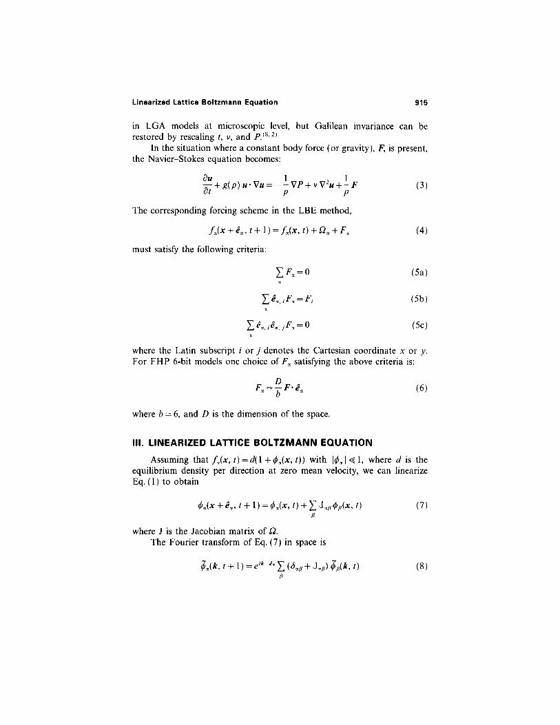
in LGA models at microscopic level, but Galilean invariance can berestored by rescaling t, v, and P.(8, 2)

In the situation where a constant body force (or gravity), F, is present,the Navier-Stokes equation becomes:

The corresponding forcing scheme in the LBE method,

must satisfy the following criteria:

where the Latin subscript i or j denotes the Cartesian coordinate x or y.For FHP 6-bit models one choice of Fx satisfying the above criteria is:

where b = 6, and D is the dimension of the space.

III. LINEARIZED LATTICE BOLTZMANN EQUATION

Assuming that fx(x, t) = d(1 + $x(x, t)) with | ( / x | « 1, where d is theequilibrium density per direction at zero mean velocity, we can linearizeEq. (1) to obtain

where J is the Jacobian matrix of Q.The Fourier transform of Eq. (7) in space is

916 Luo

The above equation can be written in a vector form:

where |$(k, t)> is the fluctuation vector with component f c ( k , t), i.e.,

The matrix

is the evolution operator, where

and I is the identity matrix. The diagonal matrix

is the displacement operatorThe eigenmodes of H ( k ) are the hydrodynamic and kinetic modes, and

the eigenvalues of H(k) are related to the transport coefficients of thecorresponding LGA or LBE model.(l,2) By solving the eigenvalue problemof H(k), one can study the generalized hydrodynamics of the model. (1 -3 )

IV. ANALYTIC SOLUTIONS OF LINEARIZED LATTICEBOLTZMANN EQUATION

Even though the eigenvalue problem of H(k) cannot be solved analyti-cally in general, the inverse of H(k) can always be obtained exactly. There-fore, one can obtain analytic solutions for some flows in which the bound-ary conditions and forcing are simple. Although the procedure to obtainthe solution of LLBE (with appropriate boundary conditions) is general, itwill be illustrated using the 6-bit collision-saturated nondeterministic FHPmodel, including all possible two-, three-, and four-body collisions. In thiscase, H0 is a circulant matrix(11) and is given by:

where h1 = 1 -d(1 + 3d), h2 = d(1 + 4d)/2, h3 = d/2, h4=-d(1+d), andd = d ( 1 - d ) .


Assuming that the system is driven by a time-independent force, whoseFourier transform is | F ( k ) y = ( F 1 ( k ) , F2(k),..., F6(k))T, and that a time-independent solution exists:

then Eq. (9) becomes:

The solution of the above equation is

Therefore, by specifying | F ( k ) y (or |F(x)> equivalently), one can alwaysobtain |?(k)> analytically, as well as the flow profile. In what follows, twosimple flows are analyzed: the Poiseuille flow and the plane Couette flowin the two-dimensional space.

A. Poiseuille Flow

The Poiseuille flow is the uniformly forced flow between two parallelplates.(12) In the following analysis, the flow (in the two-dimensional space)considered is in the interval [0, L] on the y-axis, with periodic boundaryconditions in both x and y directions. We shall apply Discrete FourierTransform (DFT) (see the Appendix or ref. 13) of a set of N discrete datapoints in the interval [0, L], and denote wN = exp(i2n/N), 8y = L/N,ky = kn, and y = nL/N. For the sake of convenience, we also assume L = 2.

The forcing function in the Poiseuille flow is a square-wave functionalong x-axis, i.e., F[x) = F(y) x, where

That is, | F ( y ) y = | e c , x > F(y), where

For the above forcing function, the DFT of F(y) is:

918 Luo

Therefore, the DFT of the x-momentum, px, is

where k is orthogonal to the direction of forcing, F. Henceforth,

where

and

are the eigenvalues of H0 corresponding to the two kinetic modes ofH0.( l , 2) Therefore, from Eqs. (17), (18), and (19), and with y = (2n + 1)/N,where ne {0, 1,..., N— 1}, we obtain (see details in the Appendix):

where

and Ly = /3 N/2 is twice of the channel width between the two plates inlattice gas simulation.


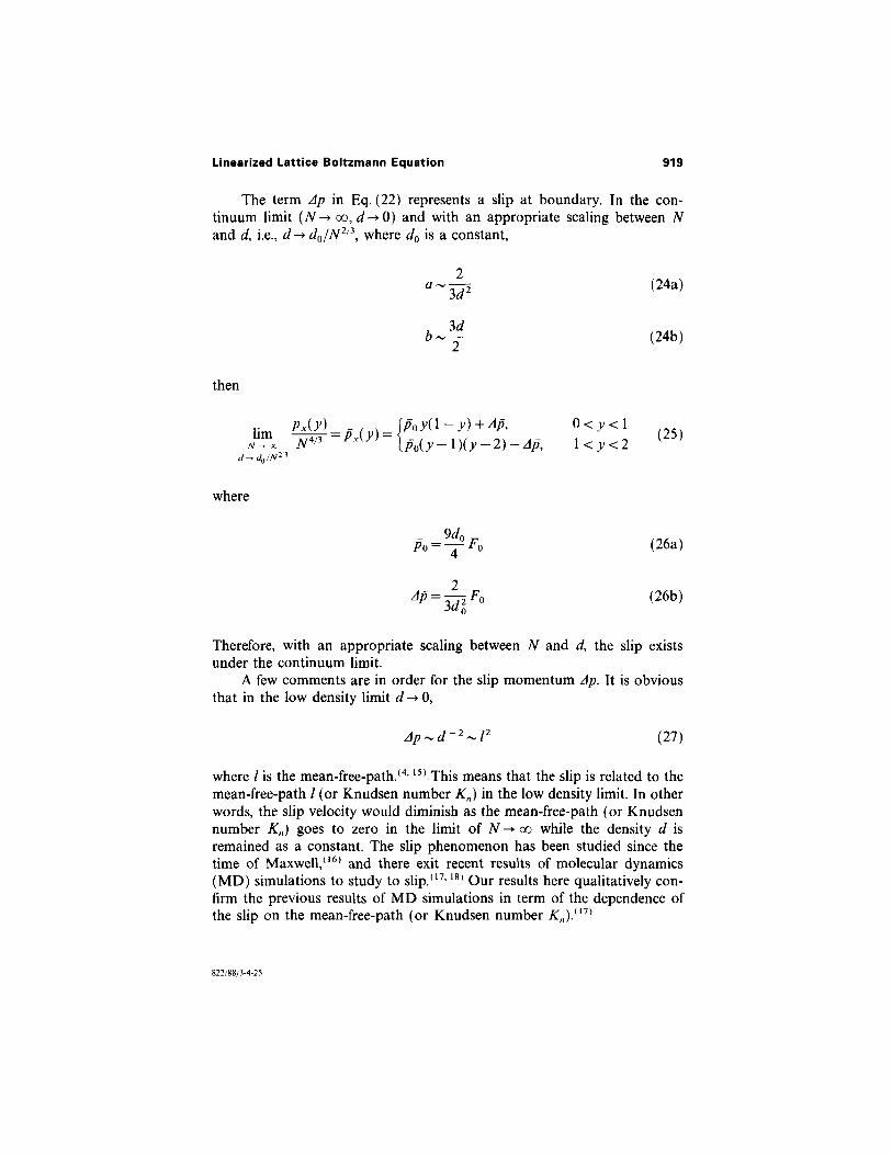
The term Ap in Eq. (22) represents a slip at boundary. In the con-tinuum limit ( N - > oo, d->0) and with an appropriate scaling between Nand d, i.e., d->d0/N2 / 3, where d0 is a constant,

then

where

Therefore, with an appropriate scaling between N and d, the slip existsunder the continuum limit.

A few comments are in order for the slip momentum Ap. It is obviousthat in the low density limit d -»0,

where / is the mean-free-path.(4,15) This means that the slip is related to themean-free-path l (or Knudsen number Kn) in the low density limit. In otherwords, the slip velocity would diminish as the mean-free-path (or Knudsennumber Kn) goes to zero in the limit of N -> oo while the density d isremained as a constant. The slip phenomenon has been studied since thetime of Maxwell,(16) and there exit recent results of molecular dynamics(MD) simulations to study to slip.(17, 18) Our results here qualitatively con-firm the previous results of MD simulations in term of the dependence ofthe slip on the mean-free-path (or Knudsen number Kn) . ( 1 7 )

822/88/3-4-25

920 Luo

B. Plane Couette Flow

The plane Couette flow is the flow between two parallel plates movingin opposite directions with constant speeds. In the case considered here, thetwo plates move in opposite directions, but with the same speed. Theforcing term for the plane Couette flow is

The DFT of the above forcing function is

Then, the DFT of the x-momentum is

and the inverse DFT of the x-momentum across the channel is (see detailsin the Appendix):

and a and b are given by Eq. (20). Again, the above equation shows thatthe momentum profile has a slip (discontinuity) at wall. Similar to thePoiseuille flow, the slip exits under the continuum limit N-> oo andd-> d0 /N1 / 3 , where d0 is a constant,

where y = (2n +1) /N ,ne{0 ,1 , . . . , N - 1 } ,

where p0 and Ap are given by Eq. (26), with a different d0. The distinctionbetween the plane Couette flow and the Poiseuille flow in the continuumlimit is that the scaling between N and d is different under the continuumlimit. This difference is apparently due to the difference in the forcing: Forthe Poiseuille flow the forcing is two-dimensional, whereas for the Couetteflow it is one-dimensional.

V. NUMERICAL RESULTS

Numerical simulations with 6-bit FHP LGA model are performed totest the accuracy of the linearized theory. The analytic results are comparedwith results of LGA simulations. The setup of the LGA simulation for thePoiseuille flow is as follows: The plates are placed parallel to the velocitydirection ( e 1 ) and periodic boundary conditions are applied. The systemsize is Nx x Ny = 512 x 32. The forcing is a square-wave function betweenthe plates. It is of uniform magnitude on sites 1 < y < Ny/2 and of oppositeuniform magnitude on sites NY/2 + 1 < y < Ny.

For the LGA simulations, the microscopic rules of applying uniformbody force are described in Fig. ( 1 ) . The uniform body force is achieved byassigning a random number r, 0 < r < 1, to each site at each time step, aftercollision and advection process have taken place, the microscopic forcingrules described in Fig. 1 are executed if r < r0 and if the rule is allowed at aparticular site. The forcing magnitude, F0, is related to the probability r0 by

Fig. 1. Forcing rules of FHP 6-bit models. In the left column are the states before theforcing. Those in the right column are after forcing. Each successful application of the forcingrule adds one unit of momentum to the system. The solid arrows indicate occupied stateswhile the hollow ones indicate vacant states. States not indicated may be either occupied orvacant.


922 Luo

for the forcing rules of Fig. l.(8) Upon each successful forcing application,the system gains one unit of momentum in the x direction. The momentumprofile is obtained by averaging over x direction and an interval of timeafter a number of iterations initially.

In Fig. 2, the momentum profile of the forced flow between parallelplates (the Poiseuille flow)(12) from the above analysis and LGA simula-tions are compared. Note that, in Fig. 2, the discontinuity of the momen-tum profiles at the boundaries (the slip momentum) is accurately predictedby the analysis. This phenomenon is a manifestation of the kinetic effectdue to a finite mean-free-path.(17, 18)

In Fig. 3, the momentum profile of the plane Couette flow from theabove analysis and LGA simulations are compared. The arrangement forthe LGA simulation of the Couette flow is the same as for the Poiseuilleflow, but the uniform forcing is only applied on two rows: y = 1 andy = N/2+ 1, with the same magnitude and opposite directions. The systemsize for this simulations is Nx x Ny = 16384 x 32. The momentum profileis obtained by averaging over x direction and an interval of time after anumber of iterations initially. Although the slip along the boundary is wellcaptured by the theoretical analysis, a systematic discrepancy between theanalytic result (straight line) and the numerical result from the LGA

Fig. 2. Momentum profile of Poiseuille flow for density per l ink d = 0.2 and a channel widthof 16 lattice sites. The system size is Nx x Ny = 512 x 32. To obtain a steady state, 106 timeiterations were run before the averaging. The momentum px is averaged over Nx and over2x 106 time iterations. The analytic result of Eq. (22) is represented by the solid line and theLGA simulation by D. The graph is rescaled so that pmax = 1. Note the agreement for thenon-zero momentum at the walls (slip velocity) due to finite mean free path. The simulationwas run on a CRAY Y-MP, with the forcing magnitude F0 ~ 1.0641 x 10-3.


Fig. 3. Momentum profile of plane Couette flow for density per l ink d=0.2 and a channelwidth of 16 lattice sites. The system size is Nx x Ny = 16384 x 32. The probability of applyingforcing is 0.06. To obtain a steady state, 103 time iterations were run before the averaging. Themomentum, px, is averaged over Nx and over 2 x 103 time iterations. The analytic result ofEq. ( 3 1 ) is represented by the solid line and the LGA simulation by " x " and " + ". The graphis rescaled so that pmax = 1. The simulation was run on a CM-200 computer.

simulation (plus signs) is observed. The discrepancy can be attributed tothe linearization of the collision operator, which is the only approximationmade in our analysis.

VI. CONCLUSION AND DISCUSSION

The analysis and numerical findings presented here confirm what hasbeen found in molecular dynamics simulations in terms of the dependenceof the slip momentum on mean-free-path l or Knudsen number Kn.(17, 18)

Our theoretical analysis is also consistent with the theoretical results inref. 19. In more general terms, our results demonstrate that hydrodynamicsdoes apply quantitatively in very small scales comparable to the mean-free-path in the system.(20, 21) However, kinetic effects are also visible in thesmall scales. Furthermore, it has been shown that, for both the Poiseuilleflow and the plane Couette flow modeled by lattice-gas automata, velocityprofiles for the both flows consist a part which satisfies the Navier-Stokesequation, and a part (the slip at wall) which is due to the kinetic effect ofa finite mean-free-path and cannot be described by the Navier-Stokesequation.(12)

In conclusion, solutions of the linearized lattice Boltzmann equationfor simple flows can be obtained analytically with the method described in

924 Luo

this paper. The kinetic effects due to a finite mean-free-path have beenanalyzed quantitatively, and accurate agreements with LGA simulationswere found. The method described here can certainly be applied to otherLGA or LBE models in two or three dimensions.

APPENDIX: DISCRETE FOURIER TRANSFORM

The discrete Fourier Transform (DFT) of a set of N data points,fn =f(xn), in the interval xe [0, L], is defined as

where fk =f(k), and WN = exp(i2n/N). The inverse DFT is

If N is even and fn + N/2 = —fn, then

With the following results,

and with the substitutions of M = N/2 and r = w2k + 1, we can obtain thefollowing DFT's for 0 < k < N/2 - 1:


and the following inverse DFT's for 0 < n < N/2 — 1:

With the above results and the substitution of y = (2n + 1 )/N, the results ofmomentum profiles in Section IV can be easily obtained.

ACKNOWLEDGMENTS

The author would like express his gratitude to Dr. Gary D. Doolen forhis ever-lasting support, guidance, and encouragement. The author espe-cially likes to thank Prof. D. d'Humieres for his diligence in reviewing thispaper and his helpful comments and suggestions regarding the DFT. Theauthor would also like to thank Dr. Shiyi Chen for his support of thiswork, Dr. Hudong Chen, Prof. Y. C. Lee, and Dr. H. Rose for manyenlightening discussions, and Mr. Dean Prichard for proof-reading thismanuscript. This work first appeared in the author's Ph.D. thesis.(2)

REFERENCES

1. L.-S. Luo, H. Chen, S. Chen, G. D. Doolen, and Y. C. Lee, Phys. Rev. A 43:7097 (1991).2. L.-S. Luo, Ph.D. thesis, Georgia Institute of Technology, 1993.3. S. P. Das, H. J. Bussemaker and M. H. Ernst, Phys Rev. E 48:245 (1993).

926 Luo

4. P. Grosfils, J. P. Boon, R. Brito and M. H. Ernst, Phys. Rev. E 48:2655 (1993).5. O. Behrend, R. Harris and P. B. Warren, Phys. Rev. E 50:4586 (1994).6. U. Frisch, B. Hasslacher, and Y. Pomeau, Phys. Rev. Lett. 56:1505 (1986).7. S. Wolfram, J. Stat. Phys. 45:471 (1986).8. U. Frisch, D. d'Humieres, B. Hasslacher, P. Lallemand, Y. Pomeau, and J.-P. Rivet,

Complex Systems 1:649 (1987).9. G. D. Doolen, editor, Lattice Gas Methods for Partial Differential Equations

(Addison-Wesley, Redwood City, CA, 1990).10. G. R. McNamara and G. Zanetti, Phys. Rev. Lett. 61:2332 (1988).11. P. J. Davis, Circulant Matrices (Wiley, New York, 1979).12. L. P. Kadanoff, G. R. McNamara, and G. Zanetti, Complex Systems 1:791 (1987).13. W. H. Press, S. A. Teukolsky, W. T. Vetterling, and B. P. Flannery, Numerical Recipes in

Fortran (Cambridge, New York, 1992), 2nd Edition, Chapter 12.14. K. Huang, Statistical Mechanics (Wiley, New York, 1963).15. M. Ernst and T. Naitoh, J. Phys. A 24:2555 (1991).16. J. C. Maxwell, Philos. Trans. Roy. Soc. London 170:231 (1879).17. D. K. Bhattacharya and G. C. Lie, Phys. Rev. Lett. 62:897 (1989).18. G. Mo and F. Rosenberger, Phys. Rev. A 42:4688 (1990).19. I. Ginzbourg and P. M. Adler, J. Phys. 11 France 4:191 (1994).20. B. J. Alder and W. E. Alley, Phys. Rev. A 1:18 (1970).21. B. J. Alder and W. E. Alley, Phys. Today 37(1):56 (1984).

Analytic Solutions of Linearized Lattice Boltzmann Equation for Simple Flows

Documents

Transcript of Analytic Solutions of Linearized Lattice Boltzmann Equation for Simple Flows