NCAR/TN-398 + STRNCAR TECHNICAL NOTE

December 1994

A Description of the

Fifth-Generation Penn State/NCAR

Mesoscale Model (MM5)

Georg A. Grell1

Jimy Dudhia2

David R. Stauffer3

MESOSCALE AND MICROSCALE METEOROLOGY DIVISION

2NATIONAL CENTER FOR ATMOSPHERIC RESEARCHBOULDER, COLORADO

1FORECAST SYSTEMS LABORATORY,NATIONAL OCEANIC AND ATMOSPHERIC ADMINISTRATION

BOULDER, COLORADO

3DEPARTMENT OF METEOROLOGY,THE PENNSYLVANIA STATE UNIVERSITY

UNIVERSITY PARK, PENNSYLVANIA

1.

II

Table of Contents

Preface . . ...........

Acknowledgments ..............

Introduction ......... .... ....

Governing equations and numerical algorithms

Chapter 1

Chapter 2

2.1

2.2

2.2.1

2.3

2.4

2.5

2.5.1

2.5.2

2.6

2.6.1

2.6.2

2.6.3

2.7

Chapter 3

3.1

The hydrostatic equations .. ....

The nonhydrostatic equations . .Complete Coriolis force option ..

Nonhydrostatic finite difference algorithms

hydrostatic finite difference algorithms

Time splitting ........

The nonhydrostatic semi-implicit schemeThe hydrostatic split-explicit scheme . .

Lateral boundary conditions ...

Sponge boundary conditions .. ...

Nudging boundary conditions ..

Moisture variables . ...

Upper radiative boundary condition

The mesh-refinement scheme ....

The monotone interpolation routines

Overlapping and moving grids . . .

iii11

e

· * 1 ix

·. 1

.1

. . . . ... 1

. . .. . .. 10

. . . . . .. .11

. ... . . . 11

. . .. . . 13

......-16

. .. . . .. 16

. . .. . . 16

·.......· 17

·.......· 17

. . . . .. .1 20

. . . . .. .1 20

3.2 24

0

*

*

*

.

· ·* * ·* · ·

The feedback ...........

A nine-point averager .......

A smoother-desmoother .......

Chapter 4 Four-dimensional data assimilation

4.1

4.2

Chapter 5

Analysis nudging ...........

Observational nudging ........

Physical parameterizations . . . ..

Horizontal diffusion ..........

5.2 Dry convective adjustment

Precipitation physics ...........

Resolvable scale precipitation processes ....

Explicit treatment of cloudwater, rainwater, snow,

Mixed-phase ice scheme .....

Implicit cumulus parameterization schemes

The Kuo scheme .......

A modified Arakawa-Schubert scheme ..

The Grell scheme .......

Parameterization of shallow convection ..

and ic

and ice

Planetary boundary layer parameterizations . . .

Surface-energy equation .........

Net Radiative flux Rn ............

Heat Flow into the Substrate H, .........

Sensible-Heat Flux H. and Surface Moisture Flux E,

Bulk-aerodynamic parameterization .......

Blackadar high-resolution model ........

Vertical diffusion ........ .. ....

Moist vertical diffusion ............

iv

3.3

3.3.1

3.3.2

. . . . . . . .. 24

.. . . . . .. .*. 25

. . . . . . . . .. 25

26

27

5.1

33

38

38

38

39

40

40

46

47

47

51

65

70

5.3

5.3.1

5.3.1.1

5.3.1.2

5.3.2

5.3.2.1

5.3.2.2

5.3.2.3

5.3.3

5.4

5.4.1

5.4.1.1

5.4.1.2

5.4.1.3

5.4.2

5.4.3

5.4.4

5.4.5

73

73

74

78

78

78

80

84

86

* 0 * * * * * * *

· · · a *

* v

* v

* v

5.5

5.5.1

5.5.2

Appendix 1

Appendix 2

Appendix 3

Appendix 4

Atmospheric radiation parameterization

Longwave radiation .........

Shortwave radiative scheme .....

Glossary of symbols .......

Look-up table for transmissivity

Map Projections .........

Land-Use categories .......

References ............

v

87

87

90

92

111

112

116

117

9 0 & a 0

0 a 0 a 0

a 0 0 0 0 0 0 a

0 a

· a a * * *

I

PREFACE

This technical report describes the fifth generation Penn State/NCAR Mesoscale

Model, or MM5. It is intended to provide scientific and technical documentation of

the model for users. Source code documentation is available as a separate Technical

Note (NCAR/TN-392) by Haagenson et al. (1994). Comments and suggestions for

improvements or corrections, are welcome and should be sent to the authors.

vivii

ACKNOWLEDGMENTS

A large number of scientists, students, and sponsors, too numerous to mention, have

made significant contributions towards developing and improving this model. We would

like to thank everyone who directly implemented changes and corrections into the code, as

well as everyone who helped to identify errors and problems.

We would also like to extend our gratitude to the two reviewers (Prof. Tom Warner,

and Dr. Jian-Wen Bao), whose comments improved the manuscript significantly.

Computing for this model development was undertaken on the CRAY YMP at NCAR,

which is supported by the National Science Foundation.

The writing of this technical document was in part supported by the Department of

Energy through grant DEA105-90ER61070, and the California Air Resouces Board through

subcontract AG/990-TS05-S02 from Alpine Geophysics.

ix

1. Introduction

This technical report is a description of the fifth-generation Penn State/NCAR

Mesoscale Model (MM5). It is based on the original version described by Anthes and

Warner (1978). Although- a few of the following details of this model are well represented

in Anthes et al. (1987), extensive changes and increases in options have occurred. For

completeness, those parts that have changed little or none will also be represented here.

The document structure is as follows. In section 2 we will describe the governing equations,

algorithms, and boundary conditions. This will include the finite difference algorithms

and time splitting techniques of both the hydrostatic and the nonhydrostatic equations

of motion (hydrostatic and nonhydrostatic solver). All subsequent sections will describe

features common to both solvers. Section 3 will discuss the mesh-refinement scheme,

section 4 the four-dimensional data-assimilation technique, and section 5 will focus on the

various physics options.

2. Governing equations and numerical algorithms

2.1 Hydrostatic model equations

The vertical c-coordinate is defined in terms of pressure.

P - PtPP - Pt

where p. and pt are the surface and top pressures respectively of the model, where pt is a

constant.

The model equations are given by the following, where p* = p' - pt

Horizontal momentum;

ap*u 2 [ap*uu/m + 9pvu/m ap*qua

&t : z [ + Oy J - o'

Fc9ap*MP- Pz + + p*fv + D(2.1.1)

p*v _ 2 8p*uv/m Op*vv/m 1 8p*v_t = Om + Oy J O

- m p + ] -P p fu + D, (2.1.2)I~~~~ I * fu +D1

Temperature;

Op*_T 2 r p*uT/m Op*vT/m _ p*T&

apt a + ay -

+ p -+ pP + DT, (2.1.3)pcp cp

where the D terms represent the vertical and horizontal diffusion terms and vertical mixing

due to the planetary boundary layer turbulence or dry convective adjustment. The heat

capacity for moist air at constant pressure is given by cp = Cpd(l + 0.8qg), where qv is

the mixing ratio for water vapor and Cpd is the heat capacity for dry air.

Surface pressure is computed from

Op* _m2 ap*u/m 9p*v/m 9p* (2 1.4)a~t = - m + ay ] (2.1.4)

which is used in its vertically integrated form

oa = _2 p* u/m pv/m da. (2.1.5)at "axy Ja

Then the vertical velocity in a-coordinates, b, is computed from (2.1.4) by vertical

integration. Thus

= -4 [ [ + m2 (a + a /m)] d', (2.1.6)

P JoL at 9x ay

where a' is a dummy variable of integration and &(u =0) = 0.

In the thermodynamic equation, (2.1.3), w = d and is calculated from

w = p*a + d(2.1.7)

wheredp* = r-a + p[u + avU.l (2.1.8)dt 9t ax 9- + y Jay

The hydrostatic equation is used to compute the geopotential heights from the virtual

temperature, T,:

aln(o _ / ) -RTv g + p1 (2.1.9)9ln~a +p^ Pt /P* + qv..

2

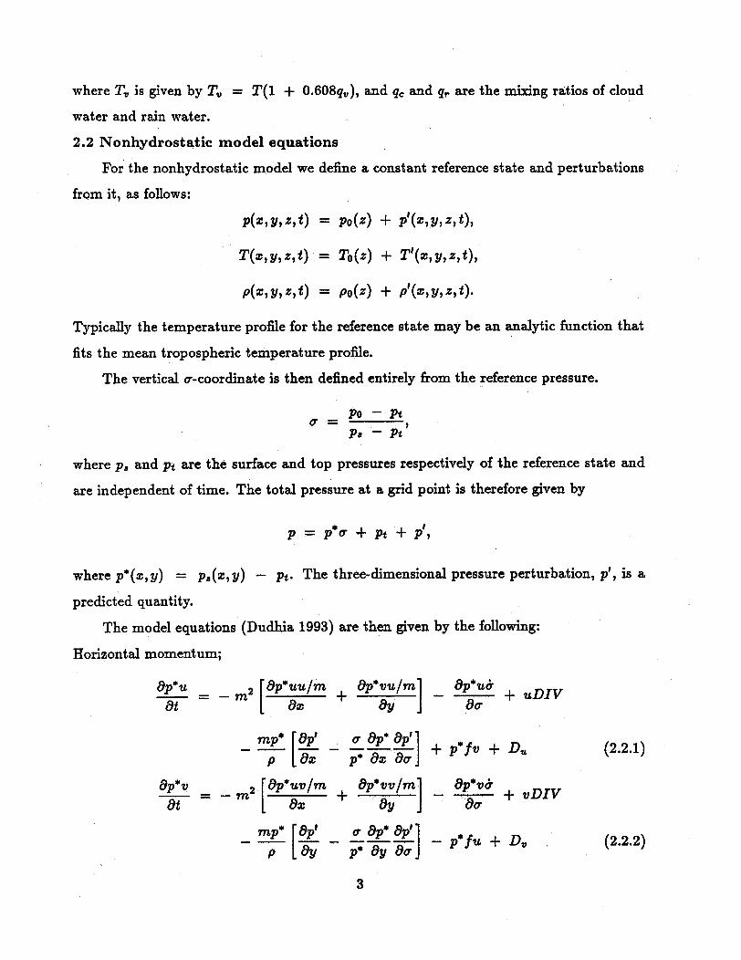
where Tv is given by TV = T(1 + 0.608qV), and qc and q, are the mixing ratios of cloud

water and rain water.

2.2 Nonhydrostatic model equations

For the nonhydrostatic model we define a constant reference state and perturbations

from it, as follows:

p(x,y,z,t) = po(z) + p'(A,y, ,t),

T(x,y,z,t) = To(z) + T'(z,y,z,t),

p(x,y,z,t) = po(z) + p'(x,y,z,t).

Typically the temperature profile for the reference state may be an analytic function that

fits the mean tropospheric temperature profile.

The vertical a-coordinate is then defined entirely from the reference pressure.

Po - PtPu - Pt

where p. and Pt are the surface and top pressures respectively of the reference state and

are independent of time. The total pressure at a grid point is therefore given by

P = p*r + pt + p,

where p*(x,y) = pa(x, ) - Pt. The three-dimensional pressure perturbation, p', is a

predicted quantity.

The model equations (Dudhia 1993) are then given by the following:

Horizontal momentum;

ap*U _ 2 rap*u/ +m p* vu/m apu- la. + j - uDIVQt 9x ay a9

mp a9p a p*O-p p-axau- ]-- -+ p[ 8v + Du Z (2.2.1)p [9x p* 9x 9aa

ap*v 2 rapuv/m ap*vv/m] + Dt m + + vDIV

9t a9x 9 jy Jau

mp* \9p' r)p* 9p']~- p-- --- -I, --- ~ - p fu + DLf (2.2.2)

P 1y p* ay aI J3

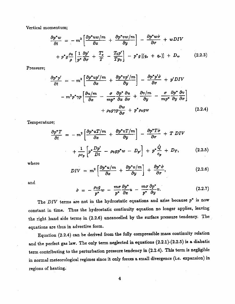
Vertical momentum;

ap*w _ 22[9p*uw/m ap*vwu/m ap*wrO -m = M -+ ay - q- wDIVat 49 8x 9 j

+ P 9 a1p p + T - pPO - g [(qC + q,)] + Dw (2.2.3)

Pressure;

app _ m 2 [ap*up'/m apvpm _ app +

M2 p au/m a ap* 9u av/m a p* avax m a a ay p- a-- m+ y[-mp ax' 8a- avY m* a y aa]

aw+ Pog9P- + P*Pogw (2.2.4)

Temperature;

ap*T 2 ap*uT/m + p*VT/m _ p*Tr m + + T DIV

at ax ay ao

+ P* - pgp* - DP# + p* + DT, (2.2.5)PCp Dt cp

where49p*p'u/, 8p~v/m 1O p*

DIV = + + (2.2.6)ax ay J au

andnno Tnr 49p*11 MO- op*Pa = p pU - rn ap. (2.2.7)p p* ax p* ay

The DIV terms are not in the hydrostatic equations and arise because p* is now

constant in time. Thus the hydrostatic continuity equation no longer applies, leaving

the right hand side terms in (2.2.6) uncancelled by the surface pressure tendency. The

equations are thus in advective form.

Equation (2.2.4) can be derived from the fully compressible mass continuity relation

and the perfect gas law. The only term neglected in equations (2.2.1)-(2.2.5) is a diabatic

term contributing to the perturbation pressure tendency in (2.2.4). This term is negligible

in normal meteorological rgimes since it only forces a small divergence (i.e. expansion) in

regions of heating.

4

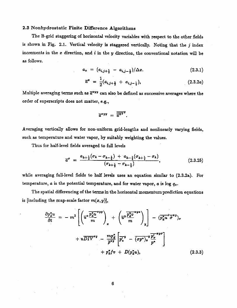
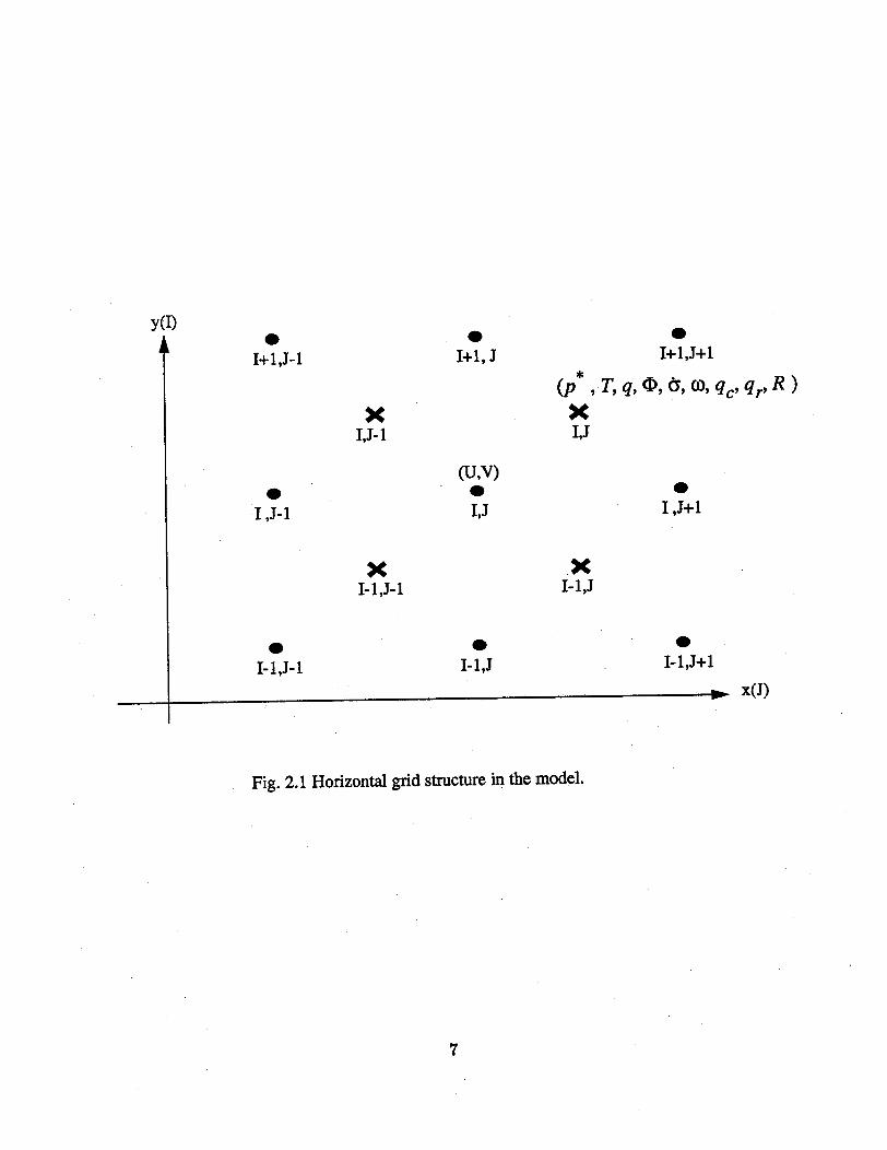
2.3 Nonhydrostatic Finite Difference Algorithms

The B-grid staggering of horizontal velocity variables with respect to the other fields

is shown in Fig. 2.1. Vertical velocity is staggered vertically. Noting that the j index

increments in the x direction, and i in the y direction, the conventional notation will be

as follows.

a, = (aij+ - aj-)/^x. (2.3.1)

1K = '(ai + + ai, ) (2.3.2a)

Multiple averaging terms such as VY can also be defined as successive averages where the

order of superscripts does not matter, e.g.,

Averaging vertically allows for non-uniform grid-lengths and nonlinearly varying fields,

such as temperature and water vapor, by suitably weighting the values.

Thus for half-level fields averaged to full levels

- ak+}(o'k-c,.- .k_) + aki(Ok+ -I- k)a + t2i(a h-2)+ a2--(o+ 2 T b- ) (2.3.2b)

(ah+ 1 - 01 I)

while averaging full-level fields to half levels uses an equation similar to (2.3.2a). For

temperature, a is the potential temperature, and for water vapor, a is log q,.

The spatial differencing of the terms in the horizontal momentum prediction equations

is [including the map-scale factor m(z, y)],

PdU - 2 [+ -U .

myy

+ uDIV\ -_ mPd [pa - P .

+ pdfv + D(plu), (2.3.3)

6

I+1, J

(U,V)

I,J

XI-1,J-1

I-1,J

I+1,J+1

(p ,T,q, to,6 qc, qr,R )XI,J

I ,J+1

XI-1,J

I-1,J+1

x(J)

Fig. 2.1 Horizontal grid structure in the model.

7

y(I)

I+ 1,J-1

xI,J-1

I ,J-1

I-i,J-l

I -lp

I -

P -v = -m i 2 P+ :( ) (]-)

at m I \

+ v.DIV' mp t - ( )p* ]

- prfu + D(pv), (2.3.4)

where p* = p*-, and DIV, the mass divergence term, is given by

DIV = m2 ( + + p,. (2.3.5)

The triple averaging in the horizontal momentum advection terms follows that of the

hydrostatic model as discussed by Anthes (1972). The subgrid-scale and diffusion operators

are represented by D(a) = KhAx2(a,,.. + a~y.y) + (Kvaz)z+ (PBL tendencies), where

the fourth-order scheme is modified to second-order near the boundaries.

The coordinate vertical velocity, a, is obtained from

r ge P- mpu- m-pr , (2.3.6)

and the vertical momentum equation is

at m - [( + ) - ( D w )

+ wDIV + P*gP pT ]

+pDIV + p w - [(T) -pp'To+ pgpg p cpT p*§(q¢ + qr)f + D(p*w). (2.3.7)

The pressure tendency equation, neglecting diabatic terms, is given by

at m M

+ p'DIV + p*pog:-- mmp* - (op~)MP, ,'

8

_Zy P09 1+ v ) ap) mp e Pm°a 2* ] (2.3.8)

and temperature tendency is differenced as

ap*T - m2 [(r P ) + (T m ) ] - (pr*T)

+T DIV + -1 [opadsg -_ D(p*p)]

+ p'- + D(p*T), (2.3.9)cp

where Dp'/Dt is differenced like the corresponding terms in (2.3.8). Moisture variables

have similar advection forms to those in (2.3.8) and (2.3.9) except when using the upstream

option where eq is replaced by the upstream value alone.

9

2.4 Hydrostatic Finite Difference Algorithms

The hydrostatic finite differencing of advection, Coriolis and heating follows (2.3.3),

(2.3.4) and (2.3.9) without the DIV terms. The pressure gradient terms in (2.3.3) become

mRT, -APG =- - R(1 + P -/Pr - (2.4.1)

and likewise for the y-gradient in (2.3.4). The surface pressure tendency is found from the

integration over all (KMAX) layers of thickness 6a(k),

KMAX= fm 2 +) + &)(k). (2.4.2)

k=1 J

Then - is found from downward integration,

(k+) = (k) p* 6cr(k) _ m2 (+ ( ) ( )(k)~-(k+ ~) = b(l) - 0t p. , (2.4.3)Ot p* p'

using the upper boundary condition that r(kc = 1) = 0. The adiabatic term in (2.3.9),

represented by the second set of terms in square brackets, becomes p*w in the hydrostatic

model, where w is defined by

dp = m9*r (2.4.4)= dt = p + a ( + mu + my (2.4.4)

The integration of the hydrostatic equation to obtain geopotential height, 4, in the

hydrostatic model is done as follows.

6 = -RTr6ln(a +pt/p*), (2.4.5)

where

L -1 + +v -Jq + q,.

and allows for water loading when the explicit moisture scheme is used. Because s is

required on the velocity levels (half-levels), it has to be integrated first between the surface,

where o = 1 and 4 = gh (h is the terrain height above sea-level), and the lowest half-level

using (2.4.5) with just the lowest-level values T,, qt, qc, qr. At all other levels (2.4.5) uses

vertical averaging between two levels.

10

The temporal differencing in the hydrostatic and nonhydrostatic models consists of

leapfrog steps with an Asselin filter. With this time filter, splitting of the solution often

associated with the leapfrog scheme is avoided. It is applied to all variables as

a = (1 - 2v)at + v(at+l + &t-), (2.4.6)

where & is the filtered variable. The coefficient v in the model is 0.1 for all variables. For

stability, diffusion terms are evaluated on the variables at time t - 1, as are the terms

associated with the moist physical processes.

2.5 Time splitting

In both the nonhydrostatic as well as the hydrostatic numerics, a time splitting scheme

is applied to increase efficiency. Because the nonhydrostatic equations above are fully

compressible, they permit sound waves. These are fast and require a short time step for

numerical stability. For the hydrostatic equations, fast moving external gravity waves are

the limiting factor. The techniques described next are designed to split these fast moving

waves from the rest of the solution.

2.5.1 The nonhydrostatic semi-implicit scheme

For the nonhydrostatic equations it is possible to separate terms directly involved with

acoustic waves from comparatively slowly varying terms, and to handle the former with

shorter time steps while updating the slow terms less frequently. The reduced equation

set for the short time step makes the model more efficient. The separated equations only

contain interactions between momentum and pressure and can be written as:

Horizontal momentum;

au m [a ap* apI1 = (2.5.1.1)at ' p[8ax P* ax 9a

atV P m p a- Aa]^ =+ S, (2.5.1.2)9t p [9y p* ay 9aa

Vertical momentum;at _ po9 ag + -P = S (2.5.1.3)At p pp A 7 p

Pressure;

9p 2 lau/m a ap* au av/m a 9p av'-a- p ap* 9 + mp* y aat ax MP , ax '90 ay Mp* ay a a

11

Po gTP awP- P - - pogw = Spt, (2.5.1.4)p* O~ -poW = $,

where the S terms contain advection, diffusion, buoyancy and Coriolis tendencies. These

are kept constant during the sub-steps. Note that only part of the p'/p term is in (2.5.1.3),

where the rest has been absorbed in the buoyancy term that contributes to S,.

The method of solution follows the semi-implicit scheme of Klemp and Wilhelmson

(1978) for the short time step. Starting with u,v,w,p' known at time r, first the two

horizontal momentum equations are stepped forward to give u 1+ and v'+l which are then

used in the pressure equation, giving a time-centered explicit treatment of horizontally

propagating sound waves. Vertical propagation of sound waves is treated implicitly by

making w 1+l and pr+l1 depend upon time-averaged values of p' and w respectively in

(2.5.1.3) and (2.5.1.4). For instance, where p' appears in (2.5.1.3) it is represented by

1 gT+1 1- =X 1(1 + +)p +(1 - p,

2 2

and similarly for w in (2.5.1.4). The parameter fi determines the time-weighting, where

zero gives a time-centered average and positive values give a bias towards the future time

step that can be used for acoustic damping. In practice, values of = 0.2 - 0.4 are used.

With second-order vertical spatial derivatives the finite difference forms of equations

(2.5.1.3) and (2.5.1.4) can be combined, eliminating pr+l, into a finite difference equation

for w'7 + , which is solvable by direct recursion on a tri-diagonal matrix.

The implicit vertical differencing scheme allows the short time step to be independent

of the vertical resolution of the model, which is important for efficiency, and thus the

step only depends upon the horizontal grid length. Additionally, the divergence damping

technique of Skamarock and Klemp (1992) is used to control horizontally propagating

sound waves. This method is similar to using time-extrapolated pressure terms in (2.5.1.1)

and (2.5.1.2), where in practice the extrapolation is about 0.1 Ar.

Temperature and moisture are predicted using the normal leapfrog step, At, because

they have no high-frequency terms contributing to acoustic waves. The slow terms for

momentum and pressure contained in the S-terms above are also evaluated on these

leapfrog steps, but for these variables the march from t - At to t + At is split into typically

four steps of length Ar during which momentum and pressure are continually updated.

12

2.5.2 The hydrostatic split-explicit scheme

When numerically solving the hydrostatic equations of motion, the stability criterion

is severely limited by external gravity waves. These are very fast moving gravity waves

that are small in amplitude (quasi-linear) and contain only a small fraction of the total

energy. Hence they change slowly over the time scale of the Rossby waves. Because of this,

splitting methods have been developed to split these fast waves from the solution (similar

also to the above method for the nonhydrostatic equations to split sound-waves). From

all the existing different options, we have chosen a method developed by Madala (1981).

This scheme separates the terms governing the gravity modes from those governing the

Rossby modes. The term "split" here refers to the separation of the motion in terms of

eigenmodes. Similar to the nonhydrostatic method, the equations are rewritten in finite

difference form asaPu, + 6b = Au, (2.5.2.1)

atBit+6$=Av, (2.5.2.2)

-P5 T + M2 D = AT, (2.5.2.3)at

ape+ N 1 .D = O,and (2.5.2.4)

$ = Mi * T. (2.5.2.5)

where the right hand sides change slowly over the time scale of the Rossby-waves. Matrices

M 1 , M2, and vector N1 are independent of x, y, and t. Notice the similarity to the

nonhydrostatic splitting method (equations 2.5.1-2.5.4). However, rather then integrating

the "fast" terms on a small time-step directly, the method described below only computes

correction terms to the equations, making this process extremely efficient. To illustrate

this, we follow Madala (1981). From the governing equations he derives equations for the

mass divergence D and the generalized geopotential A. They are

-+ [6 + 6I = :Au + 6yA (2.5.2.6)dt

and

-+M3 -D=MlAT. (2.5.2.7)at

13

Integrating equations (2.5.2.1-2.5.2.3) from t - At to t + At, where At is the time step of

the slow Rossby modes, one gets

pu(t + At) - p,u(t - At) + 2At6z = 2AtAu(t), (2.5.2.8)

p.v(t + At) - pav(t - At) + 2AMt6, = 2AtA((t), (2.5.2.9)

p.T(t + At)- p.T(t - At) + 2AtM2' = 2AtAT(t), (2.5.2.10)

where the operator () for the split-explicit scheme is defined as

mATP = t ,(t- At + nA),

n=l

where m = A. Denoting with superscript ez solutions computed using only the explicit

time integration over 2At, equations (2.5.2.8-2.5.2.10) can be written as

p.u(t + At) + 2At6, l -[ (t)] = pau'Z(t + At), (2.5.2.11)

pv(t + At) + 2At6[4- /(t)] = pveZ(t + At), (2.5.2.12)

p,T(t + At) + 2AtM2[D - D(t)] = p.Te:(t + At). (2.5.2.13)

Here Qi(t) and D(t) have been computed using the explicit time integration over 2At.

Similar, for the pressure tendency we can write

P.(t + At) + 2AtN . [D - D(t)] = P(t + At). (2.5.2.14)

To find equations for the correction terms on the left hand side of equations (2.5.2.11-

2.5.2.13), the divergence and geopotential equations (2.5.2.6-2.5.2.7) are then solved over

the the small time-steps using

[D(t + (n + 1)A) - D(t)] - [D(t + (n - )Ar) - D(t)]

+ 2Ar(62 + 6)[$(t + nAr) - (t)] (2.5.2.15)

1= I[De,(t + At) - D(t - At)]M"

14

and[4(t + (n + 1)Ar) - 4(t)] - [(t + (n - 1)Ar)- $(t)]

+ 2AlrM3[D(t + nAr) -D(t)] (2.5.2.16)

= [ e,(t + At) - (t - At)77TI

The correction terms themselves are integrated in equations (2.5.2.15)and (2.5.2.16), and

then added to equations (2.5.2.11-2.5.2.14).

AT, the timestep of the fast modes, of course varies with the mode. For a clean

separation of the modes, a vertical normal mode initialization developed and applied to the

MM4/MM5 system by Errico (1986) is used at the beginning of the model run to calculate

the vertical modes. In MM5, only the external and the fastest internal mode are being

considered with different time steps. This allows the time-steps of the slow tendencies to

be twice as large as they were with the previously used Brown-Campana (1978) algorithm,

and they are comparable to the ones used in the nonhydrostatic numerics.

15

2.6 Lateral Boundary conditions for the coarsest mesh domain

2.6.1 Sponge Boundary Conditions

The sponge boundary condition is given by

= () ( ) + (1 w(n)) ( ), (2.6.1)

where n = 1,2,3,4 for cross-point variables, n = 1,2,3,4,5 for dot-point variables, a

represents any variable, MC denotes the model calculated tendency, LS the large-scale

tendency which is obtained either from observations or large-scale model simulations (one-

way nesting), and n is the displacement in grid-points from the nearest boundary (n = 1

on the boundary). The weighting coefficients w(n) for cross point variables (counting from

the boundary points inward) are 0.0, 0.4, 0.7, and 0.9, while for dot-point variables they are

equal to 0.0, 0.2, 0.55, 0.8, and 0.95. All other points in the coarse domain have w(n) = 1.

The above method cannot be used for the nonhydrostatic part of the model.

2.6.2 Nudging Boundary Conditions

The relaxation boundary condition involves "relaxing" or "nudging" the model-

predicted variables toward a large-scale analysis. The method includes Newtonian and

diffusion terms

( a ) = F(n)Fi(aLs - acMC)- F(n)F2 A 2 (ctLS - M) n= 2,3,4 (26.2)

F decreases linearly from the lateral boundary, such that

F(n) =( ) n = 2,3,4, (2.6.3)

F(n)= 0 n > 4, (2.6.4),

where F1 and F2 are given by1

F = P loA (2.6.5)

andAs 2

F2 = 5^ (2.6.6)

This method is also used for the nonhydrostatic part of the model to nudge the

pressure perturbation to the observations or larger-scale model simulations. However, for

16

the nonhydrostatic solver the vertical velocity is not nudged. It can vary freely, except

for the outermost rows and columns, where zero gradient conditions are specified. For the

velocity components, the values at the inflow points are specified in a manner similar to

the specification of temperature and pressure. The values at the outflow boundaries are

obtained by extrapolation from the interior points. These boundary values are required

only in the computation of the nonlinear horizontal momentum flux divergence terms;

They are not required in the computation of the horizontal divergence.

2.6.3 Moisture variables

Cloud water, rain water, snow, and ice are considered zero on inflow and zero gradient

on outflow. There is an option to specify the boundary values in the same way as for the

other variables (e.g., these variables may be known in a one-way nesting application).

2.7 Upper radiative boundary condition

An option in the nonhydrostatic model is the upper radiative boundary condition.

Klemp and Durran (1983) and Bougeault (1983) have developed an upper boundary

condition that allows wave energy to pass through unreflected. It can be expressed for

hydrostatic waves as

P= N (2.7.1)

where p and w are horizontal Fourier components of pressure and vertical velocity

respectively, p and N are the density and buoyancy frequency near the model top, and

K is the total horizontal wavenumber of the Fourier component. This expression should

be enforced for all components if the energy transport is to be purely upward with no

reflection.

The upper boundary condition is combined with the implicit pressure/vertical

momentum calculation. Before either value at time n + 1 is known, the values at the

top model level (wl is staggered half a grid length above pi) can be expressed as

p+l = b + aw 1+ , (2.7.2)

where the coefficient a(x,y,t) is dependent upon the thermodynamic structure and the

bottom boundary condition on w in the model column. It varies within only 5 per cent

of a constant value even with high terrain, and is also not strongly time-dependent. The

17

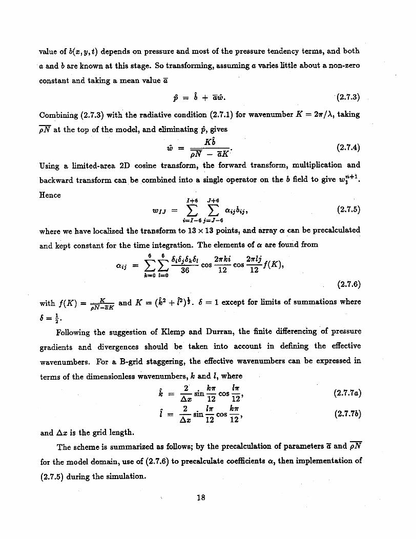
value of b(x, y, t) depends on pressure and most of the pressure tendency terms, and both

a and b are known at this stage. So transforming, assuming a varies little about a non-zero

constant and taking a mean value a

p = b + aw. (2.7.3)

Combining (2.7.3) with the radiative condition (2.7.1) for wavenumber K = 27r/A, taking

pN at the top of the model, and eliminating p, gives

AKb

w = K b - (2.7.4)pN - UaK

Using a limited-area 2D cosine transform, the forward transform, multiplication and

backward transform can be combined into a single operator on the b field to give w+ 1.

Hence1+6 J+6

w1J = E E aijbij, (2.7.5)

i=I-6 j=J-6

where we have localized the transform to 13 x 13 points, and array a can be precalculated

and kept constant for the time integration. The elements of a are found from

6 86 bi jSk61 2irki 2i1rja = - - --36 cos -1 cos 2 f(K),

k=O 1=0

(2.7.6)

with f(K) = Kp K and K = (k2 + P)i. 6 = 1 except for limits of summations wherePN I& p]K

a1

Following the suggestion of Klemp and Durran, the finite differencing of pressure

gradients and divergences should be taken into account in defining the effective

wavenumbers. For a B-grid staggering, the effective wavenumbers can be expressed in

terms of the dimensionless wavenumbers, k and 1, where

2' k2 r tir= sin cos 1 2 (2.7.7a)

2 .1r kic= Asin cos12 (2.7.7b)

Ax 12 12'

and Ax is the grid length.

The scheme is summarized as follows; by the precalculation of parameters a and pN

for the model domain, use of (2.7.6) to precalculate coefficients a, then implementation of

(2.7.5) during the simulation.

18

3. The Mesh refinement scheme

The 2-way interactive mesh refinement scheme is constructed to allow for an arbitrary

number of overlapping and translating rectangular grids with an arbitrary number of

refinement levels. The grids must be aligned with the model coordinates (no rotating

meshes), and the mesh refinement ratio of the temporal and spatial grid increments is

common for all meshes, and currently set to three. Vital parts of this refinement scheme

are the interpolation routines (Smolarkiewicz and Grell, 1992), which are used upon

initialization of new nests as well as for defining the boundaries of the fine meshes. If

the user can supply his own analysis for the finer grids (or a finer grid), the interpolated

fields can be overwritten. In the following section we describe the heart of the scheme, the

monotone interpolation routines.

3.1 The monotone interpolation routines

The most vital element of any mesh refinement scheme is an accurate and efficient

interpolation procedure. A complaint about traditional polynomial-fitting methods used

for interpolating scalar fields defined on a discrete mesh is that they often lead to spurious

numerical oscillations in regions of steep gradients of the interpolated variables. In order

to suppress computational noise, which is characteristic of quadratic and higher-order

interpolation schemes, one often implements a smoothing procedure or increased diffusion.

These, however, introduce excessive numerical diffusion that smears out sharp features

of interpolated fields. A more advanced approach invokes the so-called shape-preserving

interpolation, which incorporates appropriate constraints on the derivative estimates used

in the interpolation schemes (see Rasch and Williamson (1990) for a review). In MM5

we consider as an alternate approach a class of schemes derived from monotone advection

algorithms (Smolarkiewicz and Grell, 1992). Smolarkiewicz and Grell (1992) show that

the interpolation problem becomes identical to the advection problem, when the distance

vector is replaced by the velocity vector (see also the end of this section). Here we will

describe the implementation of the advection algorithm used in MM5. The interested

reader is referred to Smolarkiewicz and Grell (1992) for a detailed derivation of the

"advection-interpolation" equivalence.

Since shape preservation and monotonicity are important in the interpolation problem,

20

we chose the Flux Corrected Transport (FCT) scheme that uses the high-order accurate

constant-grid-flux dissipative algorithms developed by Tremback et al. (1987). We will

first describe, in abbreviated form, a general FCT algorithm, as used in MM5. Given

the exactness of the alternate-direction representation of the interpolation algorithm,

it is sufficient to consider only one-dimensional FCT schemes. Starting with the one-

dimensional advection equation in flux-form

at x ' (3.1.1)

where ' is a scalar variable advected with a flow field u(z,,t), an FCT advection scheme

may be compactly written as

4n+l- = +< -_ (Ai+l/ - Ail/2), (3.1.2)

where ( denotes a low-order, monotone solution to (3.1.1), and A is the antidiffusive flux,

limited such as to ensure that the solution (3.1.2) is free of local extrema absent in the

low-order solution. Note that

Ai+/2 = min (l,) [Ai+i/2] + mi (1,JIt+) [A + 1/ 2] (3.1.3)

where

Ai+l/2 =Fi+l/2- FLi+l/2, (3.1.4)

with FH and FL denoting fluxes from a high-order and a low-order advection scheme,

respectively. [ ]+ = ma(O, ) and [ ] _ min(0, ) are the positive- and the negative-part

operators, respectively, and

OMAX jg&n+l . In+l- OMINI, = ,AI~. + ; p,- Ao ,T + , (3.1.5a,b)AIN W . + C

where AIN, AUT are the absolute values of the total incoming and outgoing A-fluxes,

(3.1.4), from the i-th grid box, respectively. c is a small value, e.g. ~ 10 - 15, and allows

for efficient coding of a-ratios when A[N or A OUT vanish. The limiters adM A X and fM IN

define monotonicity of the scheme (i.e., by design <>M I N < o n +l < qMAX), and they are

traditionally specified (Zalesak 1979) as

pMAX a = max (O,_n, ,, + ,, in+l n+l (3.1.6a)

21

gMIN = (_,,on mn, n+l ,n+l, I+l<Pi = rnzn ^ -1, 9i s i+27 i 2; » s i-2 ) * (3.1.6b)

A shape-preserving interpolation scheme requires less restrictive monotonicity

constraints than a conservative advection scheme. The minima over 8 ratios appearing

in (3.1.3) ensure that the antidiffusive flux attributed to the i + 1/2 position on the grid

does not contribute to the generation of spurious extrema, either in gridbox i or in gridbox

i + 1. However, monotonicity of the interpolation scheme only requires that 1d+ 1 = b(xo)

is free of spurious extrema. Consequently, equation (3.1.3) may be replaced by

A+l/2 = min (1, 3) [A+/ 2 ] +min (l,) [A+ 2] . (3.1.3')

Furthermore, since the effective flow field is constant, and therefore incompressible, the

limiters in (3.1.6) may be simplified to

xMIAX = m( ; M N = mmn ( lN + l (3.1.6'a,b)

where the redundant dependence of the limiters on ^ + has been retained to ensure

strictly nonnegative values of the ft ratios in (3.1.5) (cf., Section 3.1 in Smolarkiewicz and

Grabowski, 1990). Since the low-order solution may always be written as an old value,

minus the divergence of fluxes from the low-order scheme, the entire algorithm consisting

of (3.1.2), (3.1.3'), (3.1.4), (3.1.5), and (3.1.6') is in the form of a general advection scheme.

The advection schemes used to calculate the high- and low-order fluxes for the above

equations are from Tremback et al. (1987). They derive as follows. Starting with the flux

form of the one-dimensional advection equation (3.1.1) in finite difference form

Atn+l _= + ,n + t[F- i+1/2-Fi-1/2]

rzA r -bmsi+ Sbm +m]' (3.1.7)mn m

where

m

and

F_-1/ = bmsom (3.1.9)

m22

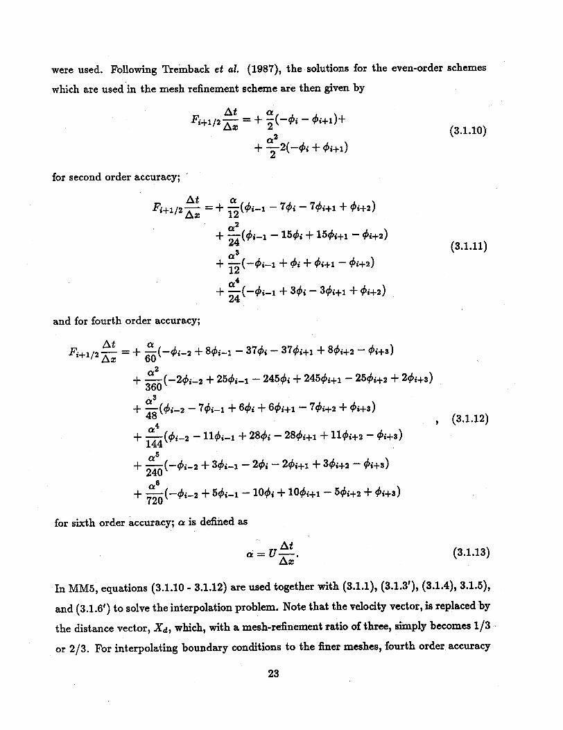
were used. Following Tremback et al. (1987), the solutions for the even-order schemes

which are used in the mesh refinement scheme are then given by

(3.1.10)

l At< a \Fill/2 A = + 2(-i - +i)+

a 2

+ -2(-Oi + oi+l)

for second order accuracy;

At aFi+/2 = + 12(i - 7i - 7i+1 + i+2)

A 2+ -(2 i - 15 + 155i + -1 i+2)

24a 3

+ 7 (-Xi-i + 4i + O+il - +2)

a 4

+ (-_i-l + 30i - 30i+1 + i+2)24

(3.1.11)

and for fourth order accuracy;

F t AFi+l/2- = + -6(-Xi-2 + 8i- -37'i- 374i+i + 8ki+2-i+60a 2

+ (-2 (-22 + 25-i1 - 245qi + 245i+l - 25ki+2 + 2i+s)360a3

+ 7-(i-2- - 7_i-i + 6•b + 6i,+l - 7i+2 + ,i+s)48 , (3.1.12)4

+ -- (i_-2 - llx-il + 28s - 28i+li + lli+2 - 1i+s)144

5+ -(-_i-2 + 3i-i - 2i - 2i+l + 3i+2 - i+3)

4+ 0a 6

+ -- (-i2 + + 0+ + - i+)

for sixth order accuracy; a is defined as

= Ata=Uz-.

Aax(3.1.13)

In MM5, equations (3.1.10 - 3.1.12) are used together with (3.1.1), (3.1.3'), (3.1.4), 3.1.5),

and (3.1.6') to solve the interpolation problem. Note that the velocity vector, is replaced by

the distance vector, X, which, with a mesh-refinement ratio of three, simply becomes 1/3

or 2/3. For interpolating boundary conditions to the finer meshes, fourth order accuracy

23

is used, while for new nest initialization, sixth order accuracy is used. While the new

nest initialization covers the whole domain, boundary interpolation is performed for the

outermost 2 rows and columns of the nest. Two rows were necessary to ensure that the

same operators were applied to each nested grid-point (including fourth-order diffusion).

3.2 Overlapping and moving grids

The mesh-refinement scheme allows for overlapping grids on the same nest-level. To

ensure numerical stability, the solution in the overlap region has to be identical. To

accomplish this, after each time-step of the grids in question, the boundary conditions

in the overlap regions are provided by the overlapping mesh. It is very important that this

procedure be performed at every timestep.

Nests can also be moved at any time in the forecast. This can be done many times,

and for any distance (integer number of grid points). The user may also move the nests

automatically if he supplies an algorithm to do so. Upon a move, a new nest initialization

is performed first. Then all high-resolution information from the previous location of the

mesh is used to overwrite the fields of the newly initialized mesh. Therefore, to ensure

best use of high resolution information, it is better to move a nest more often and for a

smaller distance.

3.3 The feedback to the coarser grids

Since the mesh refinement ratio in MM5 is set to three, a higher resolution mesh has

to be integrated three times as often as its "Mother Domain"(MD), where MD means the

coarser domain from which it gets its boundary conditions. To keep the solutions in a 2-way

interaction from diverging, the meteorological fields have to be fed back from the higher-

resolution mesh to its MD. This is done at the end of the three time-step integration.

Naturally, when this is done without smoothing or averaging, the solution on the MD

will appear somewhat noisy (diluted with small-scale information). To avoid numerical

instability, the following methods are supported in MM5 to remove non-resolvable noise

from the MD. Note that these smoothers are only applied over an interior area that is

completely determined by the higher resolution domain. It is important that input into

the nest, and feedback back to the MD does not overlap. The smoother that is used by

24

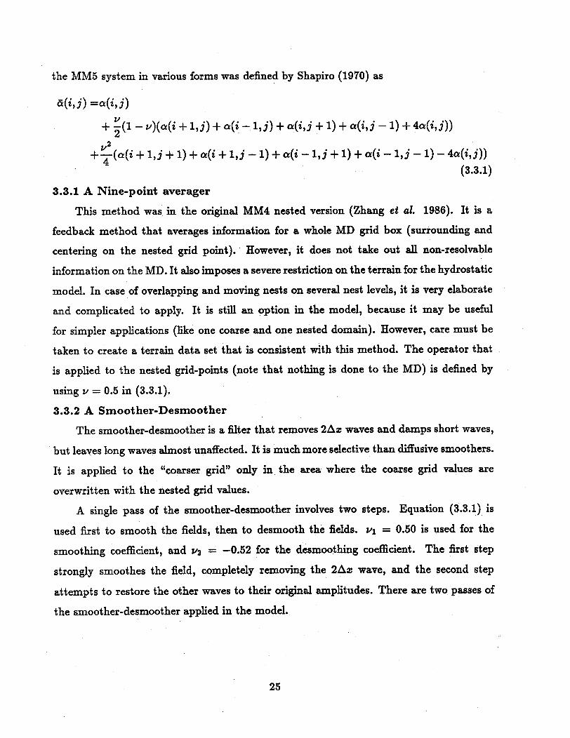
the MM5 system in various forms was defined by Shapiro (1970) as

&(ij) ==a(i,j)V

+ (1 - v)(a(i + 1,j) + a(i - 1,j) + a(ij + 1) + a(i,j - 1) + 4a(i,j))

+ (a(i + 1j + 1) + a(i + 1,j - 1) + a(i - 1,j + 1) + a(i - 1,j -1) - 4a(i,j))

(3.3.1)

3.3.1 A Nine-point averager

This method was in the original MM4 nested version (Zhang et al. 1986). It is a

feedback method that averages information for a whole MD grid box (surrounding and

centering on the nested grid point).' However, it does not take out all non-resolvable

information on the MD. It also imposes a severe restriction on the terrain for the hydrostatic

model. In case of overlapping and moving nests on several nest levels, it is very elaborate

and complicated to apply. It is still an option in the model, because it may be useful

for simpler applications (like one coarse and one nested domain). However, care must be

taken to create a terrain data set that is consistent with this method. The operator that

is applied to the nested grid-points (note that nothing is done to the MD) is defined by

using v = 0.5 in (3.3.1).

3.3.2 A Smoother-Desmoother

The smoother-desmoother is a filter that removes 2Ax waves and damps short waves,

but leaves long waves almost unaffected. It is much more selective than diffusive smoothers.

It is applied to the "coarser grid" only in the area where the coarse grid values are

overwritten with the nested grid values.

A single pass of the smoother-desmoother involves two steps. Equation (3.3.1) is

used first to smooth the fields, then to desmooth the fields. vl = 0.50 is used for the

smoothing coefficient, and v = -0.52 for the desmoothing coefficient. The first step

strongly smoothes the field, completely removing the 2Ax wave, and the second step

attempts to restore the other waves to their original amplitudes. There are two passes of

the smoother-desmoother applied in the model.

25

4. Four Dimensional Data Assimilation (FDDA)

The concept of combining current and past data in an explicit dynamical model

such that the model's prognostic equations provide time continuity and dynamic coupling

among the various fields has become known as four-dimensional data assimilation (FDDA).

Current interest in the use of FDDA in mesoscale models, for either model initialization

(dynamic initialization) or for use of the model as an analysis/research tool (dynamic

analysis), is a logical extension of the traditional link between objective analysis methods

and dynamic relationships.

Currently, two major types of FDDA are used operationally and in research. The first

is an intermittent process of initializing an explicit prediction model, using the subsequent

forecast (typically 3-12 h) as a first guess in a static three-dimensional objective analysis

step, and then repeating the process for another forecast cycle. The second is a continuous

(every model time step) dynamical assimilation where forcing functions are added to the

governinga model equations to gradually udge" the model state toward the observations.

This continuous nudging type of FDDA is used in the PSU/NCAR modeling system.

Nudging was first developed and tested at Penn State by Kistler (1974), under Prof. J.

Hovermale, and by Anthes (1974), and Hoke and Anthes (1976). See Stauffer and Seaman

(1990) for an historical overview of the technique.

Nudging or Newtonian relaxation is a relatively simple but very flexible technique:

the data used for nudging can be of any type, measured or derived, analyzed to a grid for

assimilation into the model or inserted as individual observations. Gridded analyses of the

observations that are assimilated can be obtained by successive correction, variational, or

statistical optimal interpolation (OI) techniques, and the weights used when nudging to

individual observations can be simple Cressman-type (distance-weighted) functions or more

complicated statistical functions based on OI. It can be shown that successive corrections,

OI, and variational approaches are all fundamentally related to the "idealized analysis"

and thus to each other. In fact, nudging is basically a successive-correction technique which

uses a numerical model to include the time dimension.

The method of Newtonian relaxation or nudging relaxes the model state toward

the observed state by adding, to one or more of the prognostic equations, artificial

26

tendency terms based on the difference between the two states. The model solution can be

nudged toward either gridded analyses or individual observations during a period of time

surrounding the observations. These two techniques, hereafter referred to as "analysis

nudging" and "obs nudging", respectively, can be used individually or simultaneously on

any MM5 model grid. For guidance in selecting which nudging technique(s) to use for

your particular application, as well as suggested parameter specifications, see Stauffer and

Seaman (1990), Stauffer et al. (1991) and Stauffer and Seaman (1993).

4.1 Analysis Nudging

The analysis-nudging term for a given variable is proportional to the difference between

the model simulation and an analysis of observations calculated at every grid point. The

general form for the predictive equation of variable a(x, t) is written in flux form as

cdp*aP t = F(a,x,t)+Ga*Wa(x,t) e(x).p*(&o-a)+Gp..*Wp.*Ep.(x) *a(po-p*) (4.1.1)

All of the model's physical forcing terms (advection, Coriolis effects, etc.) are

represented by F, where a are the model's dependent variables, x are the independent

spatial variables, and t is time. The second and third terms on the right of (4.1.1) are

similar in form and represent the nudging terms for a and p*, respectively. Due to the flux

form of the predictive equation, the third term appears in (4.1.1) when nudging pressure in

the continuity equation of the hydrostatic version of MM5. (Note that this term is zero in

the nonhydrostatic version of MM5 because p* is computed from the hydrostatic reference

state and is constant in time.)

With Gpo = 0, or in the nonhydrostatic version of MM5, (4.1.1) simplifies to

8p*aat = F(a,x,t) + Ga Wa * e,(x) -p*(&o - a) (4.1.2)Ot

The nudging factor Ga determines the magnitude of the term relative to all the other

model processes in F. Its spatial and temporal variation is determined mostly by the

four-dimensional weighting function, W, which specifies the horizontal, vertical and time

weighting applied to the analysis, where W = wvywwt. The analysis quality factor, e,

which ranges between 0 and 1, is based on the quality and distribution of the data used to

27

produce the gridded analysis. The estimate of the observation for a analyzed to the grid

is &o.

The nudging factor Ga is defined based on scaling arguments. Because the nudging

contribution is artificial, it must not be a dominant term in the governing equations and

should be scaled by the slowest physical adjustment process in the model (inertial effects).

Thus the Ga is usually defined to be similar in magnitude to the Coriolis parameter, and

it must also satisfy the numerical stability criterion, G, <I a. Typical values of Ga are

10-4s - 1 to 10-8s- 1 for meteorological systems, where values of Ga = 3 x 10-4s - 1 to

6 x 10-4 - 1 are usually "large enough". A value of Ga which is too large will force the

model state too strongly toward the observations. This is undesirable because (a) the

ability of the model equations to resolve mass-momentum imbalances will be decreased;

and (b) the ability of the model to generate its own mesoscale meteorological structures

(e.g. fronts, squall lines) will be impaired by heavy insertion of the observed analyses.

Such problems arise because the analyses may not resolve these mesoscale structures or

may be contaminated by observational and analysis errors. On the other hand, if Ga is

too small, the observations will have minimal effect on the evolution of the model state,

allowing phase and amplitude errors to grow.

For simplicity, if we drop the physical forcing terms F from (4.1.2), and assume

W(x,t) = 1, a- = 0 and the observational analysis is perfect and time invariant, then

= Ga(&o-a) (4.1.3)at

which has the solution

a = &o + (ai - &o)e-Gt (4.1.4)

where a, is the initial value of a at the start of the nudging period. Therefore, the model

state approaches the observed state exponentially with an e-folding time of To = Ga

,which is about 0.93 h for Ga = 3 x 10-4s-. This implies that very high frequency

fluctuations in the data, as might be available from wind profilers or Doppler radars (say,

every 5 min), would not be retained well unless Ga were much greater; but then the

nudging term may not be small compared to some terms of F.

28

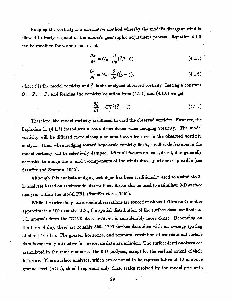
Nudging the vorticity is a alternative method whereby the model's divergent wind is

allowed to freely respond in the model's geostrophic adjustment process. Equation 4.1.3

can be modified for u and v such that

Ou aa=G, a (Go0 C) (4.1.5)

= G. .- (& -oC, (4.1.6)

where i is the model vorticity and Co is the analyzed observed vorticity. Letting a constant

G = G, = G, and forming the vorticity equation from (4.1.5) and (4.1.6) we get

= GV(co-C) (4.1.7)

Therefore, the model vorticity is diffused toward the observed vorticity. However, the

Laplacian in (4.1.7) introduces a scale dependence when nudging vorticity. The model

vorticity will be diffused more strongly to small-scale features in the observed vorticity

analysis. Thus, when nudging toward large-scale vorticity fields, small-scale features in the

model vorticity will be selectively damped. After all factors are considered, it is generally

advisable to nudge the u- and v-components of the winds directly whenever possible (see

Stauffer and Seaman, 1990).

Although this analysis-nudging technique has been traditionally used to assimilate 3-

D analyses based on rawinsonde observations, it can also be used to assimilate 2-D surface

analyses within the model PBL (Stauffer et al., 1991).

While the twice daily rawinsonde observations are spaced at about 400 km and number

approximately 100 over the U.S., the spatial distribution of the surface data, available at

3-h intervals from the NCAR data archives, is considerably more dense. Depending on

the time of day, there are roughly 500- 1200 surface data sites with an average spacing

of about 100 km. The greater horizontal and temporal resolution of conventional surface

data is especially attractive for mesoscale data assimilation. The surface-level analyses are

assimilated in the same manner as the 3-D analyses, except for the vertical extent of their

influence. These surface analyses, which are assumed to be representative at 10 m above

ground level (AGL), should represent only those scales resolved by the model grid onto

29

which they are assimilated. This is necessary to avoid difficulties related to the insertion

of small-scale divergence patterns (near 2Am) which might interact adversely with the

model's parameterizations (e.g., the moisture-convergence criterion used to determine the

existence and intensity of Anthes-Kuo convection).

Effective assimilation of single-level data depends on the equivalent depth over which

the data are inserted into the model. Beneficial effects on numerical forecasts can be

achieved by distributing single-level data throughout several model layers. This approach

requires that the data be applied in a consistent manner such that they are assured to

be representative of those layers. For example, the homogenizing effect of vertical mixing

during free convective conditions allows us to assume that surface-layer wind and mixing

ratio (q) observations can be applied throughout the model PBL according to a conceptual

model of boundary-layer structure. Such an idealized conceptual model is given by Garratt

et al. (1982) and is based on typical moderate to large instabilities observed at Wangara

and Minnesota (Fig. 4.1). However, in this same situation the frequent presence of

a shallow superadiabatic layer near the surface makes surface temperature or potential

temperature data poorly representative of the boundary layer as a whole, and similarity

relationships describing the potential temperature profile become inaccurate. The same is

true during nocturnal inversion conditions. These and other factors make assimilation of

single-level surface temperature observations unattractive for defining the temperature of

the mixed layer above the surface layer. For example, nudging towards an inaccurately

diagnosed mixed-layer temperature can cause serious errors in the simulated PBL depth or

even lead to a sudden spurious collapse of the unstable PBL structure. This can result from

assimilating a surface temperature observation which is cooler than the model-simulated

value by only a few tenths of one degree. In general, surface temperature data should not

be directly assimilated into the model (see Stauffer et al., 1991).

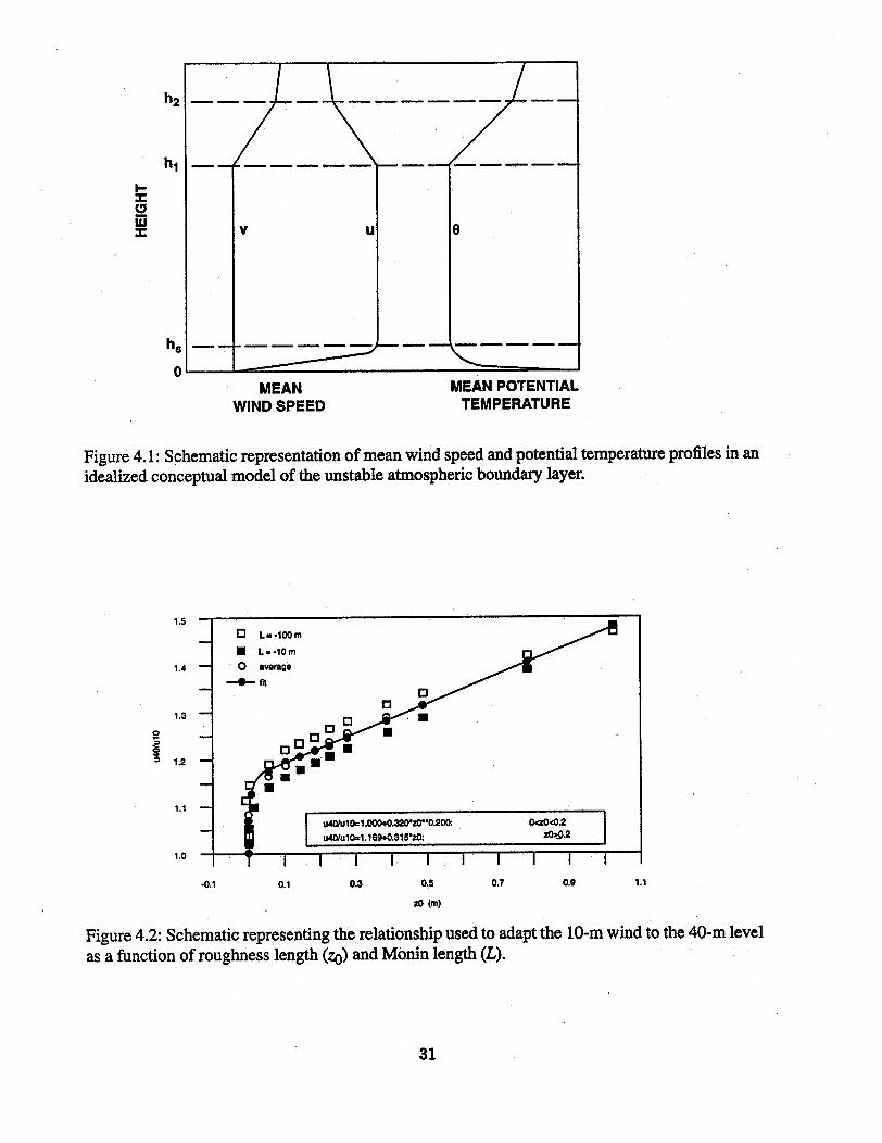
Figure 4.1 shows the unstable lower troposphere comprised of three distinct layers:

a surface layer extending to height h,, a well-mixed layer from h, to h1 and a transition

layer extending from hi to h2. With the x-axis defined parallel to the mean wind, Fig. 4.1

suggests that the v component of the wind is zero and there is thus no directional shear

through the lower two layers. The surface wind speed analysis, discussed above and

30

v u

MEANWIND SPEED

0

MEAN POTENTIALTEMPERATURE

Figure 4.1: Schematic representation of mean wind speed and potential temperature profiles in anidealized conceptual model of the unstable atmospheric boundary layer.

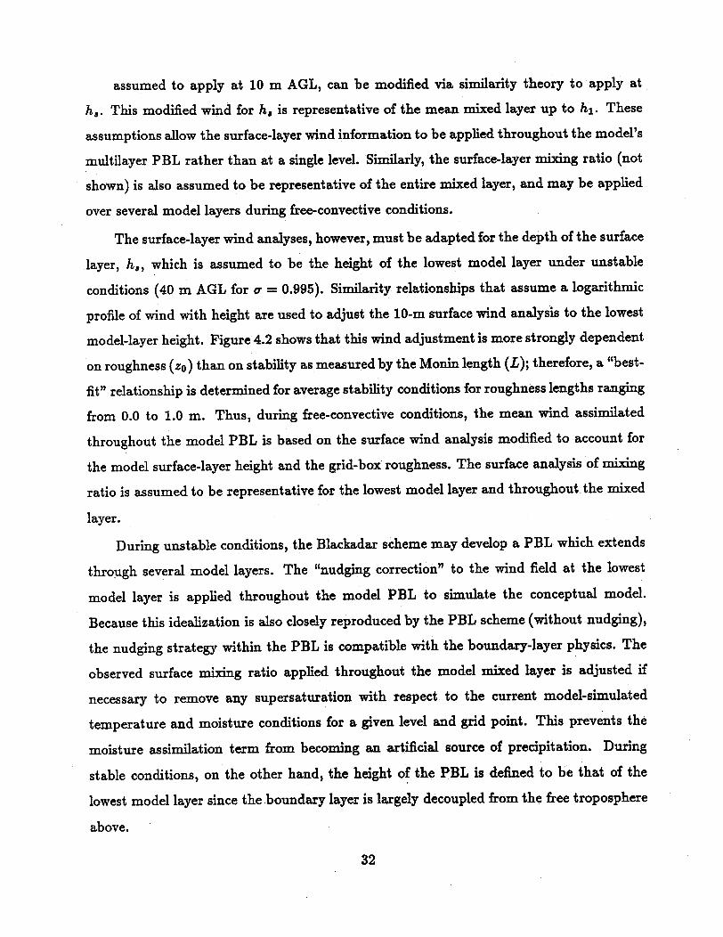
1.5

1.4

1.3

0T-

1.2

1.1

1.0

0.1 0.1 0.3 0.5 0.7 0.9 1.1

zO (m)

Figure 4.2: Schematic representing the relationship used to adapt the 10-m wind to the 40-m levelas a function of roughness length (zo) and Monin length (L).

31

I-

w

n I i I --I--"-~~~~~~~~~~

assumed to apply at 10 m AGL, can be modified via similarity theory to apply at

h8 . This modified wind for h. is representative of the mean mixed layer up to hi. These

assumptions allow the surface-layer wind information to be applied throughout the model's

multilayer PBL rather than at a single level. Similarly, the surface-layer mixing ratio (not

shown) is also assumed to be representative of the entire mixed layer, and may be applied

over several model layers during free-convective conditions.

The surface-layer wind analyses, however, must be adapted for the depth of the surface

layer, h,, which is assumed to be the height of the lowest model layer under unstable

conditions (40 m AGL for = 0.995). Simity relationships that assume a logarithmic

profile of wind with height are used to adjust the 10-m surface wind analysis to the lowest

model-layer height. Figure 4.2 shows that this wind adjustment is more strongly dependent

on roughness (zo) than on stability as measured by the Monin length (L); therefore, a "best-

fit" relationship is determined for average stability conditions for roughness lengths ranging

from 0.0 to 1.0 m. Thus, during free-convective conditions, the mean wind assimilated

throughout the model PBL is based on the surface wind analysis modified to account for

the model surface-layer height and the grid-box roughness. The surface analysis of mixing

ratio is assumed to be representative for the lowest model layer and throughout the mixed

layer.

During unstable conditions, the Blackadar scheme may develop a PBL which extends

through several model layers. The "nudging correction" to the wind field at the lowest

model layer is applied throughout the model PBL to simulate the conceptual model.

Because this idealization is also closely reproduced by the PBL scheme (without nudging),

the nudging strategy within the PBL is compatible with the boundary-layer physics. The

observed surface mixing ratio applied throughout the model mixed layer is adjusted if

necessary to remove any supersaturation with respect to the current model-simulated

temperature and moisture conditions for a given level and grid point. This prevents the

moisture assimilation term from becoming an artificial source of precipitation. During

stable conditions, on the other hand, the height of the PBL is defined to be that of the

lowest model layer since the boundary layer is largely decoupled from the free troposphere

above.

32

Therefore, the 3-hourly surface-analysis nudging is also given by (4.1.2), but the

vertical extent of the nudging is controlled by the model- simulated PBL depth, with

&o for wind and moisture adjusted as previously discussed above. The analysis confidence

factor, e, for the 3-h surface analyses, is functionally dependent on the spatial distribution

of the surface observations used to produce the analysis. Over land it varies from unity

at grid boxes within one-half the prescribed radius of influence of a surface observation to

0.2 for grid boxes outside the prescribed radius.

The vertical weighting factor, w,, is defined as

W = - R + Wa < 1. (4.1.8)

where wR and w S represent we for assimilation of 3-D rawinsonde and 2-D surface data,

respectively, and w s depends on the model-simulated PBL depth. The surface data are

assimilated with full strength (wS = 1.0) within the layers defining the PBL and with

reduced strength (w S = 0.9) one layer above (in the transition layer). The vertical

weighting function used to assimilate 3-D rawinsonde data is defined such that w = 0.0 in

the PBL, 0.1 in the transition layer and 1.0 aloft. During stable conditions, therefore, the

surface data are applied with full strength only in the lowest model layer and with reduced

strength one layer above. Both types of analysis nudging generally assimilate temporally

interpolated gridded analyses; that is, &o in (4.1.2) is interpolated in time, for example,

from either 12-h 3-D analyses or 3-h 2-D surface analyses. Therefore, we is usually set to

unity, except when decreasing the nudging at the end of a dynamic-initialization period.

4.2 Observational Nudging

This alternative scheme does not require gridded analyses of observations throughout

the case study period, and may be better suited for situations with high-frequency

asynoptic data (e.g., profilers), especially on the subalpha scales. Its form is similar to

(4.1.2) and it uses only those observations which fall within a predetermined time window

that is centered about each model time step. The set of differences between the model and

the observed state is computed at the observation locations, and analyzed back to the grid

in a region surrounding the observations. The tendency for a(x,t) with Gp. = 0 is given

33

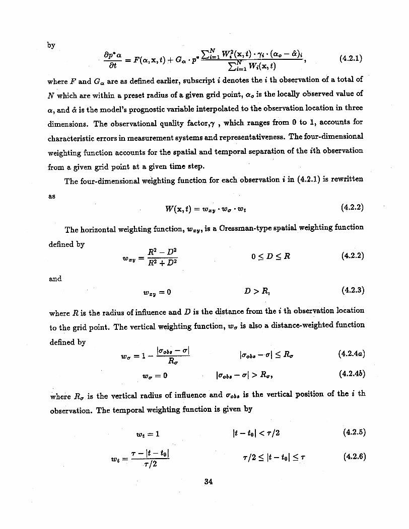
by8P* cW(x) O (C'-

Wi~a*,t+ c~pC~ ~ ?~~(1)·i·(a-d, (4.2.1)At__ - F(a,x,t) + Go .W* W (x()

where F and Ga are as defined earlier, subscript i denotes the i th observation of a total of

N which are within a preset radius of a given grid point, a, is the locally observed value of

a, and a is the model's prognostic variable interpolated to the observation location in three

dimensions. The observational quality factor, , which ranges from 0 to 1, accounts for

characteristic errors in measurement systems and representativeness. The four-dimensional

weighting function accounts for the spatial and temporal separation of the ith observation

from a given grid point at a given time step.

The four-dimensional weighting function for each observation i in (4.2.1) is rewritten

as

W(x,t) = wy * War Wt (4.2.2)

The horizontal weighting function, wy, is a Cressman-type spatial weighting function

defined by

W = / + D2 0 < D < R (4.2.2)m= R2 + D2

and

W2V= 0 D > R, (4.2.3)

where R is the radius of influence and D is the distance from the i th observation location

to the grid point. The vertical weighting function, w, is also a distance-weighted function

defined by

= 1 - obs - 1 b.oso - Al < R, (4.2.4a)R,

W = 0 Irobs - 1 > Ry, (4.2.4b)

where R, is the vertical radius of influence and oobe is the vertical position of the i th

observation. The temporal weighting function is given by

Wt = 1 It- to < r/2 (4.2.5)

W r-|to| r/2< It - t0 1 <r (4.2.6)rt/2

34

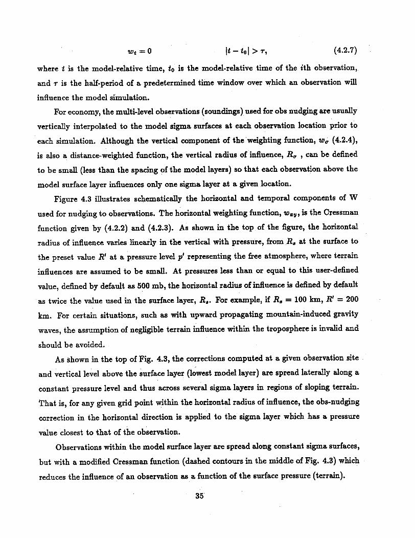
Wt = 0 It - tol > (4.2.7)

where t is the model-relative time, to is the model-relative time of the ith observation,

and r is the half-period of a predetermined time window over which an observation will

influence the model simulation.

For economy, the multi-level observations (soundings) used for obs nudging are usually

vertically interpolated to the model sigma surfaces at each observation location prior to

each simulation. Although the vertical component of the weighting function, Wa (4.2.4),

is also a distance-weighted function, the vertical radius of influence, Re , can be defined

to be small (less than the spacing of the model layers) so that each observation above the

model surface layer influences only one sigma layer at a given location.

Figure 4.3 illustrates schematically the horizontal and temporal components of W

used for nudging to observations. The horizontal weighting function, Way, is the Cressman

function given by (4.2.2) and (4.2.3). As shown in the top of the figure, the horizontal

radius of influence varies linearly in the vertical with pressure, from R. at the surface to

the preset value R' at a pressure level p' representing the free atmosphere, where terrain

influences are assumed to be small. At pressures less than or equal to this user-defined

value, defined by default as 500 mb, the horizontal radius of influence is defined by default

as twice the value used in the surface layer, R.. For example, if R, = 100 km, R' = 200

km. For certain situations, such as with upward propagating mountain-induced gravity

waves, the assumption of negligible terrain influence within the troposphere is invalid and

should be avoided.

As shown in the top of Fig. 4.3, the corrections computed at a given observation site

and vertical level above the surface layer (lowest model layer) are spread laterally along a

constant pressure level and thus across several sigma layers in regions of sloping terrain.

That is, for any given grid point within the horizontal radius of influence, the obs-nudging

correction in the horizontal direction is applied to the sigma layer which has a pressure

value closest to that of the observation.

Observations within the model surface layer are spread along constant sigma surfaces,

but with a modified Cressman function (dashed contours in the middle of Fig. 4.3) which

reduces the influence of an observation as a function of the surface pressure (terrain).

35

(*)

(A)

(-)

(.)

A

x

1

Wt

0,

B

Figure 4.3: Schematic showing the horizontal weighting function, wy, and the temporal weight-ing function, wt, used for obs nudging.

36

zf

14 Rs I-oi

I

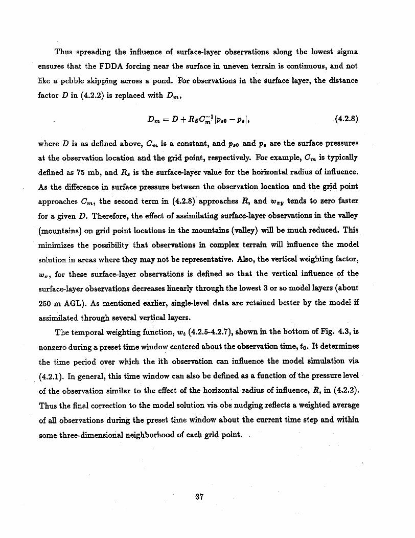
Thus spreading the influence of surface-layer observations along the lowest sigma

ensures that the FDDA forcing near the surface in uneven terrain is continuous, and not

like a pebble skipping across a pond. For observations in the surface layer, the distance

factor D in (4.2.2) is replaced with D,,

Dm = D + RsCml lpo - p. , (4.2.8)

where D is as defined above, Cm is a constant, and p.o and p, are the surface pressures

at the observation location and the grid point, respectively. For example, Cm is typically

defined as 75 mb, and R. is the surface-layer value for the horizontal radius of influence.

As the difference in surface pressure between the observation location and the grid point

approaches Cm, the second term in (4.2.8) approaches R, and w., tends to zero faster

for a given D. Therefore, the effect of assimilating surface-layer observations in the valley

(mountains) on grid point locations in the mountains (valley) will be much reduced. This

minimizes the possibility that observations in complex terrain will influence the model

solution in areas where they may not be representative. Also, the vertical weighting factor,

w,, for these surface-layer observations is defined so that the vertical influence of the

surface-layer observations decreases linearly through the lowest 3 or so model layers (about

250 m AGL). As mentioned earlier, single-level data are retained better by the model if

assimilated through several vertical layers.

The temporal weighting function, wt (4.2.5-4.2.7), shown in the bottom of Fig. 4.3, is

nonzero during a preset time window centered about the observation time, to. It determines

the time period over which the ith observation can influence the model simulation via

(4.2.1). In general, this time window can also be defined as a function of the pressure level

of the observation similar to the effect of the horizontal radius of influence, R, in (4.2.2).

Thus the final correction to the model solution via obs nudging reflects a weighted average

of all observations during the preset time window about the current time step and within

some three-dimensional neighborhood of each grid point.

37

5. Treatment of physical processes

5.1 Horizontal diffusion

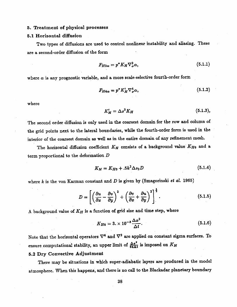
Two types of diffusions are used to control nonlinear instability and aliasing. These

are a second-order diffusion of the form

FH2a = *KHV, (5.1.1)

where a is any prognostic variable, and a more scale-selective fourth-order form

FH4M = p*KV 4, (5.1.2)

where

KH = A2KH (5.1.3),

The second order diffusion is only used in the coarsest domain for the row and column of

the grid points next to the lateral boundaries, while the fourth-order form is used in the

interior of the coarsest domain as well as in the entire domain of any refinement mesh.

The horizontal diffusion coefficient KH consists of a background value KHO and a

term proportional to the deformation D

KH KHo + .5k 2 As 2D (5.1.4)

where k is the von Karman constant and D is given by (Smagorinski et al. 1965)

_ \(9u 9v\ 2 2, (9 9u\ 2] ' gD = - a +(8 + 2] (5.1.5)

A background value of KH is a function of grid size and time step, where

KHO = 3. x 10- S (5.1.6)At '

Note that the horizontal operators V 4 and V 2 are applied on constant sigma surfaces. To

ensure computational stability, an upper limit of 6 is imposed on KH

5.2 Dry Convective Adjustment

There may be situations in which super-adiabatic layers are produced in the model

atmosphere. When this happens, and there is no call to the Blackadar planetary boundary

38

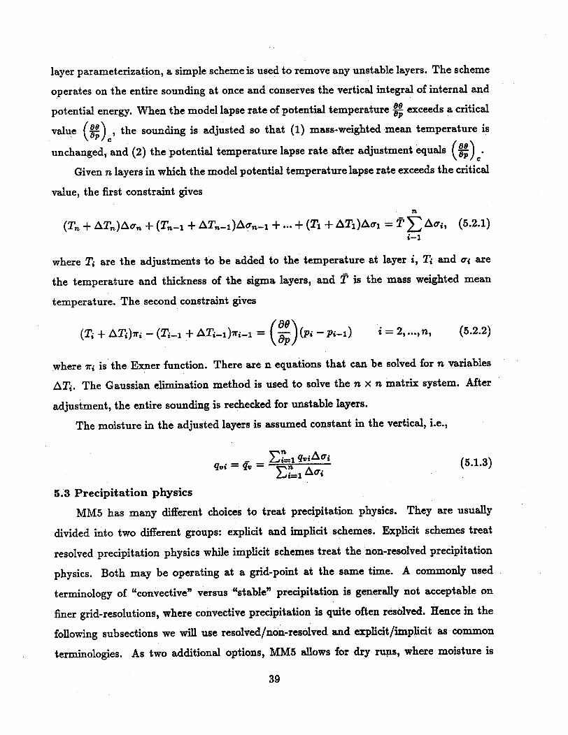
layer parameterization, a simple scheme is used to remove any unstable layers. The scheme

operates on the entire sounding at once and conserves the vertical integral of internal and

potential energy. When the model lapse rate of potential temperature |p exceeds a critical

value (a) , the sounding is adjusted so that (1) mass-weighted mean temperature ise \

unchanged, and (2) the potential temperature lapse rate after adjustment equals () .

Given n layers in which the model potential temperature lapse rate exceeds the critical

value, the first constraint gives

n

(Tn + AT,)A^n + (T- + A )- + + (TT 1 + TAT)AA< = +T Aci, (5.2.1)i-i

where Ti are the adjustments to be added to the temperature at layer i, Ti and cri are

the temperature and thickness of the sigma layers, and T is the mass weighted mean

temperature. The second constraint gives

(Ti + ATi)7ri - (T i-i + ATil )rl = ( p)(Pi - i-) i = 2,...,n, (5.2.2)

where iri is the Exner function. There are n equations that can be solved for n variables

ATi. The Gaussian elimination method is used to solve the n x n matrix system. After

adjustment, the entire sounding is rechecked for unstable layers.

The moisture in the adjusted layers is assumed constant in the vertical, i.e.,

qvi = q = 'n (5.1.3)

5.3 Precipitation physics

MM5 has many different choices to treat precipitation physics. They are usually

divided into two different groups: explicit and implicit schemes. Explicit schemes treat

resolved precipitation physics while implicit schemes treat the non-resolved precipitation

physics. Both may be operating at a grid-point at the same time. A commonly used

terminology of "convective" versus "stable" precipitation is generally not acceptable on

finer grid-resolutios convective pre itations, is quite often resolved. Hence in the

following subsections we will use resolved/non-resolved and explicit/implicit as common

terminologies. As two additional options, MM5 allows for dry runs, where moisture is

39

treated as a passive variable (no explicit and implicit schemes are applied). Another

option is a "fake dry run", where only the effects of the latent heat release are removed.

These 2 options do not require any further description and will not be discussed in the

following subsections.

5.3.1 Resolvable scale precipitation processes

These schemes are usually activated whenever grid-scale saturation is reached.

In other words, they treat resolved precipitation processes. The most simple way

that sometimes is still used on larger-scales, is to simply remove super-saturation as

precipitation and add the latent heat to the thermodynamic equation. More sophisticated

schemes carry additional variables such as cloud and rainwater (subsection 5.3.1.1), or

even ice and snow (subsection 5.3.1.2). Both schemes described next are enhancements of

MM4's original scheme (Hsie 1984).

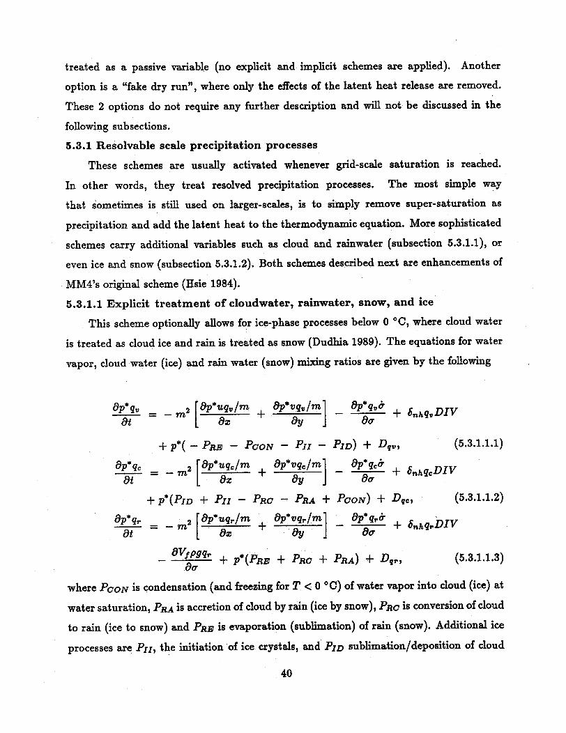
5.3.1.1 Explicit treatment of cloudwater, rainwater, snow, and ice

This scheme optionally allows for ice-phase processes below 0 °C, where cloud water

is treated as cloud ice and rain is treated as snow (Dudhia 1989). The equations for water

vapor, cloud water (ice) and rain water (snow) mixing ratios are given by the following

ap* q 2 8p*u,,/m Ap*vq,/m' apqv 6 -at =q -m L- a + 6,nhqDIVat m[ x 9y j a

+ p'( - PRE - PCON - PII - PID) + Dqv, (5.3.1.1.1)

* = -m 2 [ p*uqc/m + yp*q/m] a- +-m + + bnh- DIV9t ax 9y O y

+ p*(PID + PII - PRC - PRA + PCON) + Dqc, (5.3.1.1.2)

Oapq.r 2 [p*uqr/m + p*vq,/m] , + aqrDIVOr': + aff ykDIVOt [Ox y oa

a VfPSq + P*(PRE + PRC + PRA) + Dr, (5.3.1.1.3)

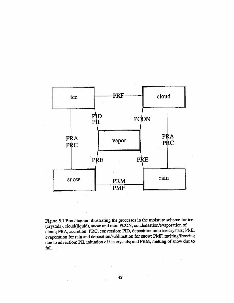
where PCON is condensation (and freezing for T < 0 °C) of water vapor into cloud (ice) at

water saturation, PRA is accretion of cloud by rain (ice by snow), PRC is conversion of cloud

to rain (ice to snow) and PRE is evaporation (sublimation) of rain (snow). Additional ice

processes are PII, the initiation of ice crystals, and PID sublimation/deposition of cloud

40

ice (Fig. 5.1). The fall speed of rain or snow is Vf. The term 6,nh is 1 for nonhydrostatic

and 0 for hydrostatic simulations.

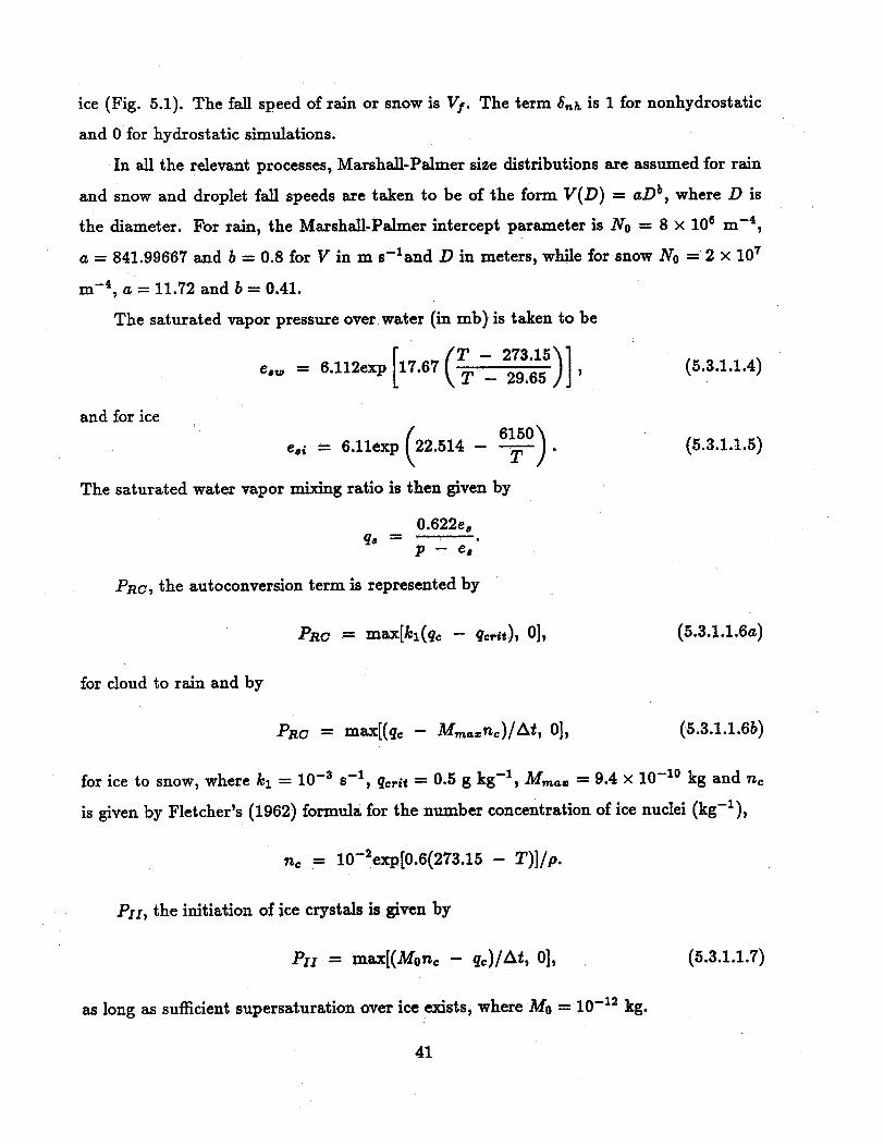
In all the relevant processes, Marshall-Palmer size distributions are assumed for rain

and snow and droplet fall speeds are taken to be of the form V(D) = aDb, where D is

the diameter. For rain, the Marshall-Palmer intercept parameter is No = 8 x 106 m 4 ,

a = 841.99667 and b = 0.8 for V in m s-land D in meters, while for snow No = 2 x 107

- 4, a = 11.72 and b = 0.41.

The saturated vapor pressure over water (in mb) is taken to be

F.~= I~nT - 273.15\1e = 6.112exp [17.67 29 65)] (5.3.1.1.4)

and for ice( 6150)

ei = 6.11exp (22.514 - 61) (5.3.1.1.5)

The saturated water vapor mixing ratio is then given by

0.622eeqq =

P - es

PRC, the autoconversion term is represented by

PRO = max[k(qc - qcrit), 0], (5.3.1.1.6a)

for cloud to rain and by

PRC = max[(qc - Mmasnc)/At, 0], (5.3.1.1.6b)

for ice to snow, where k 1 = 10- 3 s- l , qcrit = 0.5 g kg-l , Mma& = 9.4 x 10-10 kg and nc

is given by Fletcher's (1962) formula for the number concentration of ice nuclei (kg-l),

nc = 10- 2exp[0.6(273.15 - T)]/p.

PII, the initiation of ice crystals is given by

Pjr = max[(Monc - qc)/At, 0], (5.3.1.1.7)

as long as sufficient supersaturation over ice exists, where Mo = 10- 12 kg.

41

P;Dp

rpI

P J

n IU PI .

vapor

IE P]

PRMPMF

)N

P]P:

E

rain

I -- -

Figure 5.1 Box diagram illustrating the processes in the moisture scheme for ice(crystals), cloud(liquid), snow and rain. PCON, condensation/evaporation ofcloud; PRA, accretion; PRC, conversion; PID, deposition onto ice crystals; PRE,evaporation for rain and deposition/sublimation for snow; PMF, melting/freezingdue to advection; PII, initiation of ice crystals; and PRM, melting of snow due tofall.

42

P]P1

snowI I

T=

1

'J

I

cloud

I

ice I

I

� I

PRA, the accretion rate is given by

4 A3+b(5.3.1.1.8)PRA = ~rpaqcENo,(^^ , (5.3.1.1.8)

where r is the gamma-function, E is the collection efficiency (1 for rain and 0.1 for snow)

and A is given by

A = _\ r 1/4X ?rNoPe /

Here p, is the mean density of rain or snow particles (1000 and 100 kg m~3 , respectively.)

PID, the deposition onto or sublimation of ice particles is found from

4Di(Si - 1)pnA+ B

where

Si = qv/qi,

L2A = K L PT2 B -

L, is the latent heat of sublimation, K. is the thermal conductivity of air, R. is the gas

constant for water vapor, and x is the diffusivity of vapor in air. The mean diameter of ice

crystals, Di, is found from the mean mass, Mi = qc/nc, and the mass-diameter relation

for hexagonal plates from Rutledge and Hobbs (1983), Di = 16.3Mi/2 meters.

PRE, the evaporation of rain and sublimation/deposition of snow can be determined

from

2rNo(S - 1) ffi (ap) 12/3 r(5/2 + b/2)] (51110PR + f2 /+/(5.3.1.1.10)PRE= A+ B A2 ) A5/2+b/2

with the relevant No, a, and b chosen for rain or snow, and S = SW or Si. The definition

of A and B also change from the above for rain, substituting L/ for L, and qw for .,i. For

snow, 27r is replaced by 4. The values of fi and f2 are 0.78 and 0.32 for rain and 0.65 and

0.44 for snow. The term in brackets represents a distribution-integrated ventilation factor,

F = fi + f 2 Sl/SRel/2, with S, = ,t/PX, the Schmidt number, and Re = V(D)Dp/u, the

Reynolds number, and Ot is the dynamic viscosity of air.

43

PCON, the condensation is determined as follows. Temperature, water vapor mixing

ratio and cloud water are forecast first: these preliminary forecast values are designated

by T*, q* and q*. We define

6M = q- - q ,,

where q*8 is the saturated mixing ratio at temperature T*,

(1) if SM > 0 (supersaturation),

PCON = A i, (5.3.1.1.11a)At

where1

r l 1 L2=

.R- c'L, ,T* 21+ R,, Cpm T 2

(2) if SM < 0 and qc > 0 (evaporation),

o= min[-r16 Y *PaoN =-min [ T2Ap t ' t] , (5.3.1.1.11b)

(3) if SM < 0andqc = 0,

PCON = 0. (5.3.1.1.11c)

The PCON term is computed diagnostically so no iteration is needed.

Additionally, as snow falls through the 0 °C level, it immediately melts to rain. This

process is given by

PRM = -gVtq (5.3.1.1.12)Ap

Advection of ice or snow downwards or of rain or cloud upwards through this level also

melts or freezes the particles, where

PMF = w(qc + r) (5.3.1.1.13)Ap

In both cases, the 0 °C isotherm is taken to be at a full model level boundary. Melting

occurs at the level immediately below this boundary and freezing above it.

The latent heating is thus

Q = L(PRE + PID + PII + PCON) + Lm(PM + PMF), (5.3.1.1.14)

44

where L = L, for T > 0 °C and L = L, for T < 0 °C, and Lm = L - Lv.

The fall speed is mass-weighted and so is determined from

Vf = a (4 + > (5.3.1.1.15)Vf =a. 6

The fall term in (5.3.1.1.3), the rain and snow prediction equation, may be calculated on

split time-steps, At', in the explicit moisture routine. This ensures that VfAt'/Az < 1,

which is required for numerical stability. The size of At' is determined independently in

each model column based on the maximum value of VfAt/Az in the column, where At is

the model time step.

45

5.3.1.2 Mixed-Phase Ice Scheme

This scheme is based on the simple ice phase scheme described in the previous

subsection, but it does not immediately freeze or melt water and ice. Supercooled water

can exist below 0°C in this scheme, as can unmelted snow exist above 0°C. Separate arrays

are used to store vapor, cloud, rain, cloud ice and snow.

Homogeneous freezing of cloud water to cloud ice occurs immediately below -40°C

and cloud ice melts immediately above 0°C. Snow melts according to

27rNO acri bap/2)PSM = - I -- Ka(T -To) 2 + f2 I ) Sl/(5 /2+ b/2) (53.1.2.1)

Lf 1 2 + JS/22Cb/2

where fi = 0.78 and f2 = 0.31 (Rutledge and Hobbs 1984), and the other constants are

the ones relevant to snow in subsection (a). Evaporation of melting snow is modified to

use the values of A and B for rain as in (5.3.1.1.10).

Heterogeneous freezing of cloud water to cloud ice is also included following Bigg

(1953),pq

PeC = B'{exp[A'(To - T)]- 1} (5.3.1.2.2)

where A' = 0.66K - 1, B' = 100m-s - 1 and the number concentration of cloud droplets

per unit volume of air, N = 1010 m - 3.

Sekhon and Srivastava (1970) determined that better comparison against observed

snow distributions can be obtained in theoretical studies if the slope intercept value for

the size distribution is expressed as

No.(m- 4 ) = 1.05R -0 94 (5.3.1.2.3)

where, No, is the slope intercept and R (m s - 1) is the snow fall rate. Thus a variable

intercept parameter replaces the constant No, used in the simple ice scheme.

This can be expressed in terms of snow mixing ratio, qs, as

4

{ r / kl 0.94 0.94b+4

No = I1.05 [_ 2rP. ( si 1 (5.3.1.2.4)pqsc xpqs j J

where, a1 = ar4b

46

5.3.2 Implicit cumulus parameterization schemes

5.3.2.1 The Kuo scheme

In this scheme, the amount of convection is determined by the vertically integrated

moisture convergence. The feedback to the larger scale (the vertical distribution of

heating and moistening), is determined with the help of the normalized vertical profiles of

convective heating (N(cr)) and moistening (Nm(a)), and a vertical eddy-flux divergence

of water vapor associated with cumulus convection Vqf (a). Therefore, equations (2.1.3),

(2.2.5) and (5.3.1.1.1) can be rewritten to include the convective-scale fluxes as

Op*T _ 2 [Op*uT/m Op*vT/mr _p*T__

Ot a + y 9

+ p + p*- Nh()(l - b)gMt + DT, (5.3.2.1.1)PCp Cpm

Op*T _ 2 [ p*uT/m Op*vT/m p*T^r =- ^m [ Ox + 9y J ̂ ~9a^ +pT.DIV

+ 1 \p* D _ pO9 puW - DP] + pL-Nh()(l -b)gMt + DT, (5.3.2.1.2)OCt = Cpm

q -= + .DIDIVst ay a

+ P* - PRE - ON-P -PD) +P bMtNm()+p V + Dqv, (5.3.2.1.3)·qv= + 8,,hqDIVOt

where the vertically integrated moisture convergence Mt is

M= (d2) j Vp d. (5.3.2.1.4)

A portion (1 - b) of M is assumed to condense and precipitate, where the remaining

fraction b is assumed to moisten the grid column. Following Anthes(1977), b is a function

of the mean relative humidity RE of the column, where

b= 2(1- RH) (5.3.2.1.5)

for RH 2 0.5, and b = 1 otherwise.

The vertical profiles of heating and moistening

47

The normalized, nondimensional functions for the vertical profiles of heating and

moistening and the divergence of the vertical eddy flux of water vapor are subject to the

constraints

I Nh(r)da = 1,

1

j Nm(a)doa = 1,

j Vf (a)dr = 0.Jo

(5.3.2.1.6)

(5.3.2.1.7)

(5.3.2.1.8)

Anthes et al. (1987) assume simple relationships for these functions, which are

derived from budget studies. For the convective heating profile, Nh, they observe that

the convective heating often has a parabolic shape with a maximum in the upper half of

the cloud. Hence

Nh((,) = alx2 + a 2X + a3,

x = Inco

(5.3.2.1.9)

(5.3.2.1.10)

with the boundary conditions:

Nh(Oc) = 0, at Xb = Inab, and zu = (lnra (5.3.2.1.11)

at cloudbase (ab) and cloud top (C,), and

ONh(o)NIa) -(,) = ,h 490. d(5.3.2.1.12)

at a, which is defined as_ Zu + zb

2 (5.3.2.1.13)

where subscripts u and b stand for the top and the base of the cloud. Using (5.3.2.1.6), al

can be shown to be2 r o

1 - 3 2 2 t+ -zu Xb + 4Xub -umb

The vertical moistening profile, N,(a), is simply given following Anthes (1977) as

Nm (O) (1 - RH(a))qs( ) (5.f,. (1 (- RH(oB))q..(',)dr'

2.1.14)

2.1.15)

48

where

Divergence of the Vertical Eddy Flux of Water Vapor Vqf(a)

The divergence of the vertical eddy flux of water vapor is defined as

TrJ.a) -VqJ (c = - 8 (5.3.2.1.16)

If one assumes a small fraction of convective cloud cover, and the cloud vertical motion a-r

is much larger than the larger-scale vertical motion, a (5.3.2.1.16) can be rewritten as

V()a = a(~Vqf((O) = - -V [Ic(qve - qv)] I1 - a 8

(5.3.2.1.17)

where qvc is the mixing ratio in the cloud.

According to Anthes (1977), the fractional coverage a is calculate using

f (l-b)sMt (5.3.2.1.18)J Wl(-w p + a)idp

which is the ratio between the grid-average condensation rate and that of a single

cloud. The term 8ajc represents the contribution to the rate of change of cloud-mixing

ratio by entrainment (Anthes 1977). Anthes et al. (1987) assume a typical value for the

denominator of approximately 4.3 x 10"-cb s~l and then rewrite (5.3.2.1.17) as

=(1 - b)gMtV,~(,,) = ~4.3 x 10-'s O~['(q'*- Q*)] ' (5.3.2.1.19)

For further simplification, Anthes et al. (1987) next assume that s also has a parabolic

shape and can be expressed as

(5.3.2.1.20)"C= C1JX 2 + C2X + Cs,

where x = Inp, and -c = 0 at cloud-top and base. Furthermore, qv - qv is assumed to

have a parabolic profile with pressure

,vc - qv = b1z 2 + b2x +bs (5.3.2.1.21)

, = 1n[(1 - c)(100 - Pt) + pt]. (5.3.2.1.22)

49

with

The procedure

The simple procedure can be summarized as follows:

1. Compute Mt from (5.3.2.1.4)

2. Check whether Mt > 3. x 10- 5 kg m - 2 s - 1 , a critical threshold value.

3. Check the model sounding for convective instability to see if convection is possible.

4. Determine cloud top and base from sounding.

5. Check whether cloud-depth is larger than a critical value (ACa > .3)

6. Calculate the normalized vertical profile functions

7. Calculate &c on the full a levels from (5.3.2.1.20)

8. Compute qv - q, from (5.3.2.1.21)

9. Calculate Vqf from (5.3.2.1.19)

50

5.3.2.2 A modified Arakawa-Schubert scheme

The version of the Arakawa-Schubert scheme used here was developed by Grell (1993).

In contrast to the original scheme (Arakawa and Schubert 1974, AS), it includes moist

convective-scale downdrafts. Other changes have been implemented to also allow the

scheme to be used successfully in mesoscale models in mid-latitudes (Grell et al. 1991).

To simplify the description we have adapted a terminology originally introduced by Betts

(1974), which splits the parameterization problem from the modeling view in three parts:

static control, dynamic control, and feedback. The static control includes usually a

cloud-model and calculates cloud thermodynamic properties, the dynamic control is what

determines the amount and location of the convection, and the feedback determines the

vertical distribution of the integrated heating and moistening.

Static control

As with all commonly used one dimensional steady state cloud models (plumes,

bubbles, or jets), our AS scheme makes use of the assumption that entrainment occurs

over the depth of the buoyant element according to the entrainment hypothesis

1 om(z) .2.m(z) z , (5.3.2.2.1)m(z) 9z r

where A. is the total net fractional entrainment rate of the buoyant element, m its mass flux

(mu for updraft, md for downdraft), and r its radius. Following AS, the dependence on the

radius is not explicitly used. However, implicitly, the radius of the cloud is assumed to be

constant. Detrainment was originally only assumed to happen at the cloud top, but this

assumption may easily be varied (Houze et al. 1979, Lord 1978) by defining a fractional

detrainment rate, oud, and rewriting (5.3.2.2.1) for the updraft of cloud type A as

1 amu(z)

/¾pu~~~~ = ~ue/-ud = ~m (z) e~9z (5.3.2.2.2)

_ 1 { ( Emui (x, Z) e5 mu (22 )2mu(Az) ) \ 9Z deJ

where Aue is the gross fractional entrainment rate, and Iu is the total net fractional

entrainment rate of the updraft. Subscripts ent and det indicate changes due to

entrainment and detrainment, respectively. Looking at the budget of a thermodynamic

51

variable in an infinitesimal layer of the updraft we get

amuau (mu\ _ 9mu

OZ - z /)- e 9z du + Sued

(5.3.2.2.3)

Together with (5.3.2.2.2) this leads to the steady state plume equation

9az = ) e(a(z) - a,(A, z)) + S,8z(5.3.2.2.4)

where a is a thermodynamic variable, the tilde denotes an environmental value, and

subscript u denots an updraft property. S stands for sources or sinks. Similarly, for

the downdraft, we can rewrite equations (5.3.2.2.2) and (5.3.2.2.4) as

AId = Atde - IAdd1 9md(z)

md(z) Az

1 md(z) (a md(( z)(9md(z) A

t9z det

and

acd(z) = -ide(a(Z) - ad(z)) + S,Oz

where subscript d denotes a downdraft property. For moist static energy

h(z) = CpT(z) + gz + Lq(z),

equations (5.3.2.2.4) and (5.3.2.2.6) simply become

h,(A, z) ,e(() - h(X, z))az

and

aOh(z = -Ide[h(z)- hd(z)].9z

Next, for the moisture budget of the updraft, we use

u = qu(X, z) + ql(X, z) (5.3.2.2.10)

Su = -comu (A,z)q(A, z). (5.3.2.2.11)

52

(5.3.2.2.5)

(5.3.2.2.6)

(5.3.2.2.7)

(5.3.2.2.8)

(5.3.2.2.9)

and

Here So is the total water that is rained out, co is a rainfall conversion parameter and

could be a function of cloud size or wind shear, ql is the suspended liquid water content of

the cloud, and q, is the water vapor mixing ratio inside the updraft. Equation (5.3.2.2.4)

can then be rewritten as

O(q A, z) + (A, )) u ( S(q z) + q( z)) = Ae((Z) - qu(A, z) - ql(A, z)) + Su.az(5.3.2.2.12)

For the downdraft, the equation for the water vapor reads

a9 qd(Z) =--de[g(Z) -- d(Z)] + Sd.oz

(5.3.2.2.13)

Sd here is a source; namely the evaporation of rain. Assuming saturation in the updraft

and downdraft, we can make use of the approximate equation

qc(A, z) = 4*1 + - I[hc(x,z) - h'()],1 +-Y

(5.3.2.2.14)

where

· 7 = (O*') p (5.3.2.2.15)

the asterisk denotes a saturated value, and he here stands for the moist static energy in the

cloud (updraft or downdraft), if saturation is assumed. Next, to arrive at a usable closure,

the up- and down-draft mass fluxes are normalized by the updraft base (mb(A)) mass flux,

and the downdraft base mo(A) mass flux of a subensemble. Hence, for the updraft,

mu(A, z) = mb(A)77u(AX z) (5.3.2.2.16)

and1 a9n(z)

tu - Iltu d =r Tu() Oz

Equivalently, for the downdraft we may write

(5.3.2.2.17)

md(z) = mo(A)Xd(A, z) (5.3.2.2.18)

and1 9 7d(Z)

I de-~ dd = ( d.z '- 77d(Z) - OZ

(5.3.2.2.19)

53

Here, mo is the mass flux at the originating level and ad, as r7u in equation (5.3.2.2.16), is

the normalized mass flux profile.

To leave only one unknown variable, we follow Houze et al. (1979) and make the

originating mass flux of the downdraft a function of the updraft mass flux and reevaporation

of convective condensate. Therefore, the condensate in the updraft

C,(A)dA = mbdA (T 7iu(AZ)Sdz)) = ImbdA (5.3.2.2.20)

is apportioned according to

Cu(A)dA = (Rc(A) + Ed(A))dA = (a(A) + f(A))Cu(\)dA, (5.3.2.2.21)

where a + 3 = 1 and Ed, the evaporation of condensate in the downdraft for cloud type

A, can be written as

EddA = mo(A)dA ( °d(A z)Sddz = I2modA./0) (5.3.2.2.22)

From equations (5.3.2.2.20-5.3.2.2.22) we see that

EddA = -CudA = md = Imbd-2 modA (5.3.2.2.23)

and hence

m(A) = ( = e()mb(A). (5.3.2.2.24)12 (A)

Here 1-,8 is the precipitation efficiency. Following Fritsch and Chappell (1980), it is made

dependent on the windshear.

To solve the above equations we need to specify boundary conditions as well as make

some arbitrary assumptions. For the updraft we assume

h,(zb) = MAX(h(z)), with < zb, and (5.3.2.2.25)

h,(, ZT) = h*(zT), (5.3.2.2.26)

where the asterisk denotes a saturation value. Similarly, for the downdraft,

hd(zo) = MIN(h(z)). (5.3.2.2.27)

54

Physically, for both updraft and downdraft, we allow for maximum buoyancy. The

boundary conditions for the updraft are different than in the original scheme, which had

a rigid dependence on the planetary boundary layer height. In the original scheme, the

mixed layer was assumed to be well mixed, and the cloud base was located on top of the

mixed layer. In semi-prognostic tests (Grell et al. 1991) large variations of moist static

energy profiles were found in very low levels of the troposphere. This was caused by cold

downdraft outflow. Naturally, the inflow to an updraft will not be a mixture of downdraft

air and the more buoyant air; it is more likely the air with high moist static energy from

the layer above the downdraft outflow. Furthermore, compensatory subsidence should only

continue to the level from which the updraft draws its air. Compensatory uplifting may

be required in very low layers of the troposphere because of the downdraft mass flux.

Feedback

The feedback to the larger-scale environment is expressed in a convenient form as

( ). =' a L, (5.3.2.2.28)

I(S Ie -_ cuFq+i - ,(5.3.2.2.29)\at , p 8z

where s is the dry static energy (s = CpT + gz). The convective-scale fluxes within a grid

box are defined as

Fs-L F, - LFi (5.3.2.2.30)

Fq+l F, + Fi (5.3.2.2.31)

where F. is the flux of dry static energy, Fq is the flux of water vapor, and Fl is the flux

of suspended cloud liquid water. These are defined as

F.(z) + J t7(A, z)[SU(A, Z) - S(z)]mb(A)dA

x (5.3.2.2.32)

-J 7d(, Z)[sd(', Z) - -(z)]mo(A)dA

AFq(z) _ + f r^(Az)[q\(AZ) - {z)\m^\)d\

A> x ~~~~~~~ ~~~(5.3.2.2.33)

- f 1d(A, z)[qd(A, z) - q(z)]mo(A)dA

A

55

AFt(z) n7,(\,z)l(,,z),mb(,)d\ (5.3.2.2.34)

X

The rainfall (convective-scale sink of cloud water) is defined as

R(z) -+ /77u(Az)co(A)l(A,)mb(A)dA

>(·li·*··A (5.3.2.2.35)

- Jr?7d(\, z)qe(, z)mo(A)dA

AX

Here qe is the amount of moisture that is necessary to keep the downdraft saturated. The

second term on the righthand sides is due to downdrafts and is zero above the downdraft-

originating level. Below the updraft-air originating level, the first term on the right-hand

sides is zero and only downdrafts affect the larger-scale environment. Below the updraft-air

originating level, the convective-scale fluxes due to updrafts are zero. Between the updraft-

air-originating level and the level of free convection (the LFC), F1 and R are set to zero.

Since no liquid water is assumed to be in the environment as the downdraft, the downward

flux due to updrafts as well as downdraft fluxes in equation (5.3.2.2.33) are zero. Schubert

(1974) showed that convection will not increase the total moist static energy per unit area

in a column. In essence, only precipitation can change the dry static energy budget and

the total mass of water vapor. All variables in the flux terms can be determined from the

equations for the static control, except mb(A). This is determined in the dynamic control,

which incorporates the closure assumption of the scheme and is described next.

Dynamic control

Arakawa-Schubert first introduced the cloud work function, which is an integral

measure of the buoyancy force associated with a subensemble. Starting with

dwu dwu dz d dw 1 d wi-= B u - Fr = -' (5.3.2.2.36)

dt dz dt dtdz 2 wu dt 2'

where Bu is the acceleration due to buoyancy and Fr the deceleration due to friction, and

multiplying equation (5.3.2.2.36) by pu(, z)w(A, z), gives

d w 2 (d Pt- = puW,(B, - Fr). (5.3.2.2.37)dt 2

56

Integrating over the depth of the updraft and using mu = puWu = mb7u yields

d I T 2ZTdt pu dz = mb(A) nB ruBdz - Du, (5.3.2.2.38)

where D is the updraft-scale kinetic energy dissipation. Equation (5.3.2.2.38) can be

written in the symbolic form

-KE = Au(A)mb(A) - Du(A), (5.3.2.2.39)dt

where Au(A) is a measure of the efficiency of kinetic energy generation inside the cloud

and is called the cloud work function. It can also be written as

Au(A)= C - n 1(A, z) (h(A, z) - h*(z))dz, (5.3.2.2.40)J P T( z ) 1+7

where 7 is defined as in equation (5.3.2.2.15). As with equations (5.3.2.2.36-5.3.2.2.38),

defining a kinetic energy generation inside the downdraft leads to

ddt- KEd = Ad ()mo (A) -Dd(A), (5.3.2.2.41)

where Ad, the measure of the efficiency of kinetic energy generation inside the downdraft,

can be written as

Ad(A) = CT( ) ,A) (h*(z) - hd(A,z))dz. (5.3.2.2.42)=J, CPT(z) 1 +7

Note that dry static energy instead of moist static energy would have to be used if

subsaturation is assumed. We can combine equation (5.3.2.2.39) and (5.3.2.2.41) and

then make use of (5.3.2.2.24) to yield

dd KEtot = Atot(A)mb(A)- Dtot(A), (5.3.2.2.43)dt

where

Atot(A) = (A) + e(A)Ad(A) (5.3.2.2.44)

is the total cloud work function which was redefined as a measure of the efficiency of kinetic

energy generation in updrafts as well as downdrafts. Next, AS separated the change of the

cloud work function into two parts: One is due to the change in the larger-scale variables

( dA LSt_ ) F(A), (5.3.2.2.45)dt Ls

57

and one is due to the modification of the environment by the clouds. Since the cumulus

feedback on the larger-scale fields is a linear function of mb, this term can be written in

the symbolic form

(dAtot ) f K(AA, )mb(A')d. (5.3.2.2.46)dt cu

A

Therefore

dAt t =F(A) + fK(A) A)mb(A)dA, (5.3.2.2.47)dt

where K(A,A') are the kernels. The kernels are an expression for the interaction

between clouds (updrafts and downdrafts). Equation (5.3.2.2.47) is solved with a linear

programming method (Lord 1978).

In the original version of the Arakawa-Schubert scheme, the fractional entrainment

rate was the parameter which characterized the cloud. In later papers, the cloud-top

detrainment level was chosen instead. If a fine vertical resolution is assumed, the second

choice will most likely be better numerically, since no interpolation is necessary at the cloud

tops. However, in the extremely unstable environment of the mid-latitudes, it is sometimes

impossible to calculate "clouds" with cloud tops in the unstable layers. Entrainment rates

would have to be extremely large to stop cloud growth. We therefore chose the fractional

entrainment rate as the spectral parameter.

The procedure

The cloud base is a function of time and space. However, at a specific grid point the

cloud base will be the same for every member of the subensemble. We also distinguish

among an updraft-air originating level, z, a downdraft-air originating level, Zo, a cloud

base level, zb (the LCL), and a level of free convection, Zbc (LFC). Here, zu is determined

from condition (5.3.2.2.25) and determines the thermodynamic properties of the updraft

from cloud type i. The air becomes saturated at zb; condensation will start, but no

convection can occur yet because the buoyancy is negative. In some instances this level

could be the same as the LFC. The LFC is of great importance since this is the level at

which the static control starts the calculations of individual convective elements. Since the

air that feeds the cloud originates below the LCL, compensatory subsidence is allowed to

reach the originating level of the updraft air.

58

For the downdraft, the originating level is also a function of time and space. If the

downdraft exists, it will always reach the surface..

For updraft and downdraft in layer k the mass budgets are defined as

e,(k, i) - d(k, i) = (,,(k + .5, i)- 7,(k - .5,i)and (5.3.2.2.48a)

ed(k,i)- dd(k,i) = rd(k + .5, i)- 7d(k -. 5,i), (5.3.2.2.48b)

where entrainment for the updraft and downdraft is defined as

e,(k,i) = ,ueAd r7 (k + .5,i) (5.3.2.2.49a)

ed(k, i) = deAzd 7ld(k - .5, i) (5.3.2.2.49b)

and detrainment is defined as

d,(k, i) = ludAZd 77u(k + .5, i)

dd (, i) = IddAZd ld(k - .5, i).

Combining the above three equations for the updraft and downdraft yields

ZfLuk - .5,i) = vui(k + .5,i)(1. + /ue ^d - /ludAZd)

(5.3.2.2.50a)

(5.3.2.2.50b)

(5.3.2.2.51a)

for the updraft and

77d(k + .5,i) = 77d(k -. 5,i)(1. + IdeAZd - ddAd) (5.3.2.2.51b)

for the downdraft. Here we define Azd = z(k + .5) - z(k -. 5). The discretized form for

the downdraft moist static energy budget reads

hd(k +.5,i)- hd(k - .5,i)ed(k,i)h(k) - dd(Iki) -- -- ^i-h-2 ) (5.3.2.2.52)

= 7d(k + .5, i)hd(k + .5, i)- d(k - .5, i)hd( - .5, i)

Using equations (5.3.2.2.48)-(5.3.2.2.51) in equation (5.3.2.2.52) leads to

h(k + .5 i) = hhd(k - .5,i)(1.- .Spc d d Azd) + ld^eAZd h(k) (hd k + .5,1 ) - (5.3.2.2.53)

1. + dcAZd - IddAZd + .5/lddAZd

59

I

I

The moisture budget for the downdraft is developed in several steps. First, the downdraft

water vapor mixing ratio before evaporation, but after entrainment, is calculated. This is

done using

qd(k - .5,i)(1. - .5ddAzd) + lideAd (k) (52.2.54)

1. + ildeAZd - AlddAZd + .5.ddAZd

Next, equations (5.3.2.2.14) and (5.3.2.2.15) give the mixing ratio, qvd, that the updraft

or downdraft would have if saturated. Hence, the amount of moisture that is necessary to

keep the downdraft from cloud type i saturated in layer k is

qe(k,i) = -[qd(k,i) - qd(k,i)]. (5.3.2.2.55)

Next we check whether the updraft produces enough rain to sustain saturation in the

downdraft by requiring that

S coAz(k) 77(k - .5, i)ql(k - .5, i) - e(i)Az(k) 77d(k + .5, i)q(k, i) > 0. (5.3.2.2.56)

If this is not the case, a downdraft is not allowed to exist.

Having defined the discretized versions of the equations from the static control, we

now can describe the procedure.

Using the larger-scale temperature and moisture fields (To,qo) at time to, and given

a functional or empirical relationship for Ad, Jde, and jAdd, the equations from the static

control are used to calculate ,, hu(z, i), hd(z, i), q,(z, i), qd(, i),7(z, i), and 7d(Z, i) for

cloud type i. These are needed to determine the total cloud work function Atot using

Atot(i) = Au(i) + eAd(i). (5.3.2.2.57)

The discretized versions of equations (5.3.2.2.40) and (5.3.2.2.42) that are used to

determine the cloud work functions for updrafts and downdrafts are

l=.top [ g i)u( )= C l·P T(k- .5 ) " 5

* (((k -1)- z(k)].5

(z(k- 1) - z(k))]

60

(5.3.2.2.59)

k=sur .

k-f-S-'o*=zo cP T(k - .5)

hd(k - .5,i)- h*(k e -. 5)

1 + 7(k - .5) )

* (z(k) - z(k - 1))

The kernels of cloud type i are by definition the changes of the cloud work functions due

to another subensemble, i'. Thus, following Lord (1978), To and qo are modified by an

arbitrary amount of mass flux, mbAt', from the i' subensemble. This is done for every

possible subensemble and can be written in the symbolic form

T'(ki) = T(k) + 6i (T(k))mlAt', (5.3.2.2.60)

q'(k,i) = q(k) + 6i, (())mbAt. (5.3.2.2.61)

The 6 terms, which are changes per unit mb(i), are easily calculated from budget

considerations as in Lord (1978). With the downdraft terms, the moist static energy

budget of layer k and cloud type i becomes

P(t) ,,(h(k,i))=9

+ (7u(k - .5,i) - e(i)7d(k - .5, i))h(k - .5)

- (r7(k + .5,i) - e(i)7d(k + .5,i))h(k + .5)

- (es(k,i) + e(i)ed(k,i))h(k) , (5.3.2.2.62)

(,ih,,(k +.5 i)+ hu(k-.,i)+ du(dki ) 2

+ ( (k i) hd(k + .5,i) + hd(k- .5,i)+ e(t)dd(k,i)- --- 2--

where e,(k,i)andd,(k,i) are the entrainment and detrainment for the updraft, and Ap(k)

is defined by Ap(k) = p(k + .5) - p(k - .5). A simple physical interpretation of the terms

on the righthand side can be understood by looking at Fig. 5.2. The first term is the

subsidence on top of the layer, the second is the subsidence on the bottom of the layer. This

subsidence is an environmental compensatory mass flux due to the updraft and downdraft

mass fluxes inside the cloud. Note that below z, the "compensatory subsidence" may be

61

and

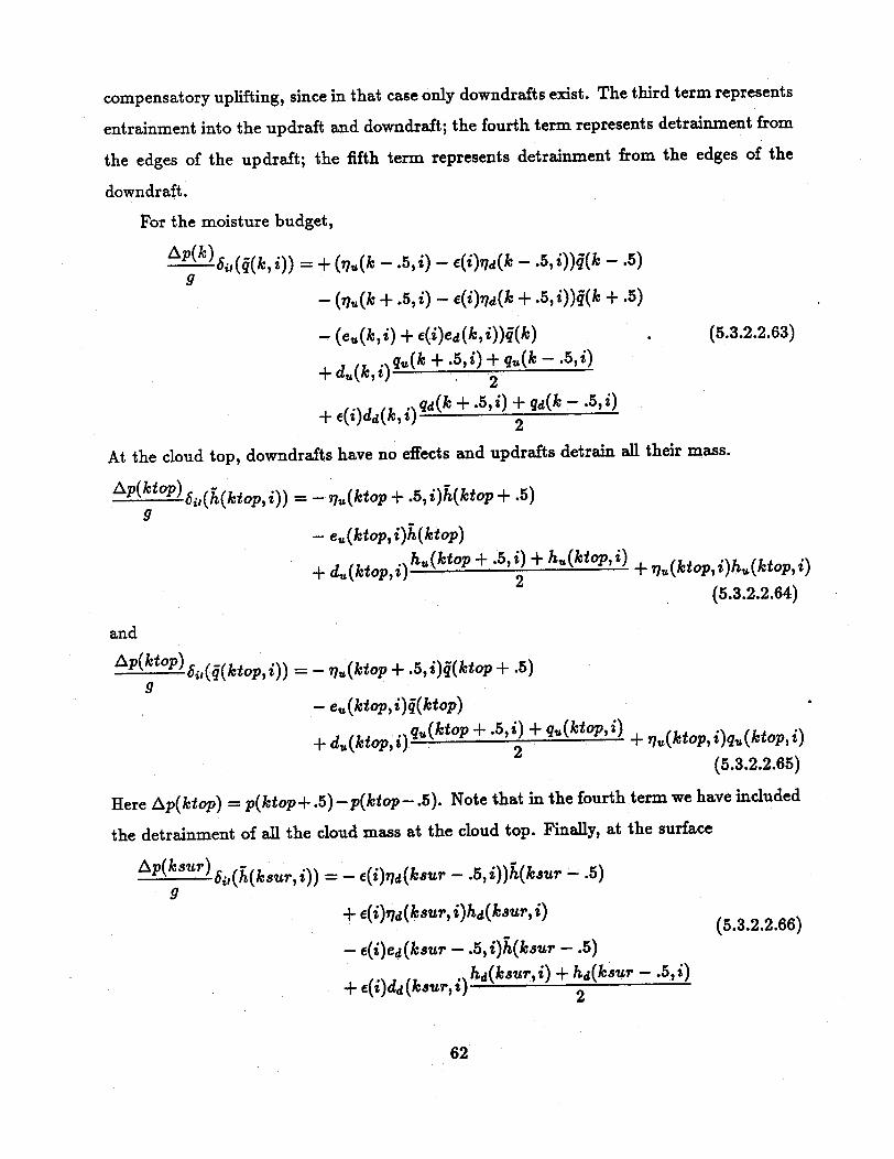
compensatory uplifting, since in that case only downdrafts exist. The third term represents

entrainment into the updraft and downdraft; the fourth term represents detrainment from

the edges of the updraft; the fifth term represents detrainment from the edges of the

downdraft.

For the moisture budget,

P(l) 6i,(4(ki)) = + (.u(k - .5,i) - (i (k - .5,i))(k - .5)9

- (.r7(k + .5, i) - e(i).d(k + .5,i))q(k + .5)

- (e(ke,i) + e(i)ed(k,i))q(k) . (5.3.2.2.63)

+ df(k i)qu(k + .5,i) + qu(k -. , i)+ duqkk, i)+ )+d-k-52,

+. ~ . gq~d(f + .5, i)+ qd(k - .5,i)+ e(i)d (kit) 2

At the cloud top, downdrafts have no effects and updrafts detrain all their mass.

Ap(ktop) 68,(h(ktop, i)) = - u(ktop + .5, i)(ktop + .5)9

- eu(ktop,i)h(ktop)

+ d(ktop,i)h( kto + .5,i) + h,(ktopi) + .n(ktop,i)h (ktop,i)(5.3.2.2.64)

and

Ap(ktoP) 6^(q(ktop, i)) = - ru(ktop + .5, i)(ktop + .5)9

- e(ktop, i)q(kop)

+ du(ktopi) q7(ktop + .5,i) + q(ktop, i) + v(ktop, i)qu(ktop, i)

(5.3.2.2.65)

Here Ap(ktop) = p(ktop+ .5) - p(ktop -. 5). Note that in the fourth term we have included

the detrainment of all the cloud mass at the cloud top. Finally, at the surface

aP(ku) S.,(h(ksuri)) = - e(i)frd(ksur - .5,i))h(ksur - .5)g

+ e(i)( r,i)hd(ur, i)(5.3.2.2.66)(5.3.2.2.66)

- e(i)ed(kur - .5,i)h(kur - .5)

(i)d(,,, d(ksur,i) + hd(ksur - .5,i)+ e(i)dd(kasur, i) 2

62

I

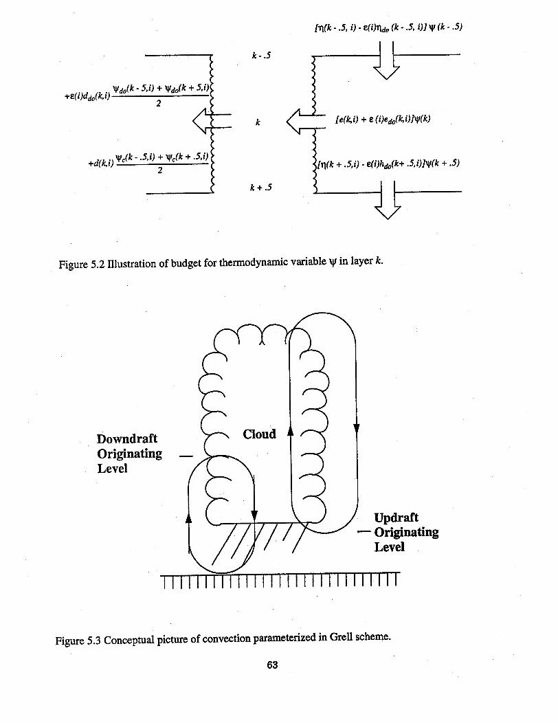
k -. 5

k

k+.5

Figure 5.2 Illustration of budget for thermodynamic variable v in layer k.

DowndraftOriginatingLevel

Figure 5.3 Conceptual picture of convection parameterized in Grell scheme.

63

.5)

raftinatingI

fil(k - .5, i) - E(i~rdo (k - .5, i)] W (k - .5)

* ^

edo(k,i)]V(k)

and

P(ku) i(q(ksur, i)) = - e(i)rd(ksur - .5,i))q(ksur -. 5)9

+ €(i)rd(ksur, i)qd(klsur, i), (5.3.2.2.7)

- e(i)ed(ksur - .5, i)q(kur - .5)

d(ksur, i) + qd(ksur - .5, i)+ e(i)dd(ksurzT,i) 2

with Ap(ksur) = p(ksur + .5) - p(ksur - .5). Here, the first term is the compensatory

environmental mass flux, the second term is the detrainment of all downdraft air at the

bottom, the third term is entrainment into the downdraft, and the fourth term is the

detrainment of air around the downdraft edges.

The new thermodynamic fields, To'(kI, i') and qo'(k,i'), are then used again from the

static control to calculate new cloud properties and a new cloud work function, A'tt(i',i).

Note that To and qo are now functions of the subensemble i'. From the definition of the

kernel we then can calculate the kernels simply as

K(i i') m= A to t ( ii)- Ao t (i) (5.3.2.2.68)

Next, we go back to the original fields and modify those with the large-scale advective

changes to get

T(k) = To+ (T) At (5.3.2.2.69)Ot ADV

and

q"(k) = qo + ( ) At, (5.3.2.2.70)a ADV

where (5.3.2.2.69) and (5.3.2.2.70) are applied over At= 30 min. The double prime

quantities are then used again by the static control, which will calculate new cloud

properties, and so new cloud work functions, Atot"(i), will be determined. Next, the

large-scale forcing (by definition the change of the cloud work function due to large-scale

effects only) is calculated using

F(i) Atot(i)- Ato(i) (5.3.2.2.71)F(;)=At

64

The large-scale forcing and the kernels are then both used by the dynamic control to

estimate the cloud base mass flux distribution function, mb, using an IMSL subroutine

to solve the linear programming problem. Finally, the feedback to the larger-scale

environment is simply given by

(at ) C 6s'(T(k))mb(i')and (5.3.2.2.72)

I q(k)( at )__ = - 6$(q(k))mb(i'), (5.3.2.2.73)

where the precipitation can be calculated using

iMAX Ck= kto

P= S 5 co^z(k)ql(k + .5,i)mu(k + .5,i)it'=1 c=l . (5.3.2.2.74)

iMAX k=kctop

- S E Az(k)qev(k + .5,i)md(k + .5,i)i'=l k=l

5.3.2.3 The Grell scheme

This is a very simple scheme that was constructed to avoid first-order sources of

errors (Grell 1993). The very simplistic conceptual picture of how this parameterization

is envisioned to function is shown in Fig. 5.3. Clouds are pictured as two steady-state

circulations, caused by an updraft and a downdraft. There is no direct mixing between

cloudy air and environmental air, except at the top and the bottom of the circulations.

The cloud model that is used to calculate cloud properties in this scheme is formulated

with only a few equations. Mass flux is constant with height, and there is no entrainment

or detrainment along the cloud edges. We can simply write

m,(z) = m,(zb) = mb ,and (5.3.2.3.1)

md(z) = md(zo) = mo (5.3.2.3.2)

for the mass flux of the updraft (m,) and the downdraft (md). Here mb and mo are simply

the mass fluxes of the updraft and downdraft at their originating level. If it is assumed that

65

the conditions at originating levels are given by the environment, for any thermodynamic

variable ,the budget inside the cloud simply becomes

au(z) = &(Zb) + Su(Z) , and (5.3.2.3.3)

(5.3.2.3.4)cd(Z) = a(zo) + Sd(z),

where a is a thermodynamic variable, the tilde denotes an environmental value, and S

stands for sources or sinks. For moist static energy

h(z) = CpT(z) + gz + Lq(z), (5.3.2.3.5)

equations (3) and (4) simply become

h,(z) = h(zb) (5.3.2.3.6)

and

hd(z) = h(zo). (5.3.2.3.7)

For the moisture budget of the updraft we can make use of the approximate equations

(5.3.2.2.14) and (5.3.2.2.15) to calculate the mixing ratio inside the cloud if saturation is

assumed. Together with equations (5.3.2.3.3) and (5.3.2.3.4), this will give us S, and Sd,

the condensation and evaporation. Note also that no cloud water is assumed to exist; all

water is converted to rain.

Given boundary conditions, equations (5.3.2.3.1)-(5.3.2.3.7) have two unknowns, mb,

and mo. In order to leave only one unknown variable, the originating mass flux of the

downdraft is made a function of the updraft mass flux and the reevaporation of convective

condensate, as in the previous section (see equations (5.3.2.2.20)-(5.3.2.2.24)). Therefore,

,lIlmbmo - - emb.

12(5.3.2.3.8)

Here, 1 - is the precipitation efficiency. To specify boundary conditions, we assume

hu(z) = h(zb)=MAX(h(z)), with z < b,and (5.3.2.3.9)

hu(zT) = h*(ZT), (5.3.2.3.10)

66

where the asterisk denotes a saturation value. Similarly, for the downdraft,

hd(z) = hd(ZO) = MIN(h(z)). (5.3.2.3.11)

Physically, for both, updraft and downdraft, we allow for maximum buoyancy. For this

deep convection scheme, the cloud base for the updraft is not restricted to the boundary

layer, but can be anywhere in the troposphere.

Feedback to the larger-scale equations

To avoid zero-order sources of errors, the feedback must include the cooling effects

of moist convective downdrafts. Furthermore, lateral mixing should never be excessive,

especially if the cloud properties have been calculated with a steady-state cloud model.

Keeping in mind the conceptual picture in Fig. 5.3, the feedback for this scheme is entirely

determined by compensating mass fluxes and detrainment at cloud top and bottom.

Conceptually, no averaging (such as the normally used top-hat or Reynolds averaging

methods) is necessary. This does not mean that scale-separation is not required, but for

this parameterization it is not necessary to assume that the fractional area coverage is

very small. Note, however, that any parameterization can only make sense if a clear scale

separation exists. None of the parameterized effects may be resolved by the larger-scale.

Assuming that the conceptual picture in Fig. 5.3 happens in only one grid box, we can

express the changes caused by the convection as

(9h(k) 9h,(z)mb 9h(z)mb hd(z)mo h(z)mo( t) a + a(5.3.2.3.12)

at -cU- 8z Oz Oz

and

9aq(k) _ 9q,(z)mb _ 9(z)mb _ qd(z)mo 84o(z)m( at ) cu~ z az a9z ^ 9+ (5.3.2.3.13)v 8z- 8z - z 8.

Because of the simplicity of the static control, these equations can be further simplified to

give

( ) =Mb (1-e) + mb( 8 ( 8 ) (5.3.2.3.14)

))+

#v )(1- ) +mb( aq(Z)-ead(Z) (5.3.2.3.15)

67

The rainfall is defined as

R = Ilmb(l -). (5.3.2.3.16)

The second term on the righthand sides of equations (5.2.2.3.14) and (5.2.2.3.15) are due

to downdrafts and are zero above the downdraft originating level. Below the updraft-air

originating level, the first term of the right-hand sides are zero and only downdrafts affect

the larger-scale environment. All variables in the flux terms can be determined from the

equations of the static control, except mb.

Dynamic control

Because of the simplicity of the above equations, many closure assumptions can be

used. The most simple closure is a Kuo-type assumption, which relates the rainfall rate

to the moisture convergence. However, more applicable seems to be a stability closure.

Again we have two choices. We could assume that the clouds will remove the available

buoyant energy as in other mesoscale parameterizations, or that the clouds will stabilize

the environment as fast as the larger-scale (or also sub-grid scale) destabilizes it, or even a

mixture of both. Although both assumptions are easily implemented, we chose the closure

which depends on the rate of destabilization. In this closure the change of the available

buoyant energy due to convection offsets the changes due to other effects (larger-scale

destabilization as well as sub-grid scale destabilization), yielding

(dABE) (^dABE) (5.3.2.3.17)dt OTH dt cu

Next, the change due to the convection is normalized in terms of the mass flux to read

( dABE B (dBE ) , (5.3.2.3.18)dt cu dt NCU

where subscript NCU denotes the change of the available buoyant energy due to a cloud

normalized by the cloud-base mass flux. Equations (5.3.2.3.17) and (5.3.2.3.18) are used

to calculate mb.

The Procedure

This section describes in detail the procedure necessary to calculate the convective

feedback. First, we will explain the very simplistic approach to calculate a normalized

feedback, then we will describe how the closure assumption determines the mass flux.

68

Using the larger-scale temperature and moisture fields (To,qo) at time to,

hl,(z),hd(z),q,(z), qd(z) are simply arrived at (see equations (5.3.2.3.6)-(5.3.2.3.10). The

first calculation is the determination of the integrals I1 and I2 (calculated as residuals

using equations (5.3.2.3.8) and (5.3.2.3.9). The next step is then to estimate the convective

changes per unit mass flux (before knowing the actual mb's). This is done by estimating

the net change of a thermodynamic variable a in a layer k by using

AP() ((k)) = (1 - e)(a(k - .5) - &(k + .5)),5g

(5.3.2.3.19)

where Ap(kl) is defined by Ap(k) = p(k+.5)-p(k-.5). This subsidence is an environmental

compensatory mass flux due to the updraft and downdraft mass fluxes inside the cloud.

Note that below zu the "compensatory subsidence" may be compensatory uplifting, since

in that case only downdrafts exist.

At the cloud top,

Ap(ktop) 6(&(ktop)) = -a(ktop - .5) + a,(ktop).9

(5.3.2.3.20)

Here Ap(ktop) = p(ktop + .5)- p(ktop - .5). Finally, at the surface (the downdraft tops)

Ap(ksur) 6( (ksur)) =(u - .5) + rd(ksur)),9

(5.3.2.3.21)

with Ap(ksur) = p(ksur + .5) - p(ksur - .5). Here, the first term is the compensatory

environmental mass flux, and the second term is the detrainment of all downdraft air at

the bottom. These normalized changes are also used in the calculation of the final feedback

(after mb is determined), which is simply given by

(a(k) ) = 6(a(k))mb. (5.3.2.3.22)

To calculate the mass flux mi, we define the buoyant energy which is available to a

cloud (updraft and downdraft) as

r g fz kb}(-b)k- ,h*( .5)ABE= CL cp T(k - .5) * -.5)))] (5.3.2.3.23)

=+or[ g * (h(kO)- h(k -5) *((k-z(k-1))pk T(k - .5) 1 + 7(k -. 5)

k=zo

69

where 7 is defined in equation (5.3.2.2.15). We can calculate ABE (similar to Lord 1982)

for the unchanged environment as well as for the environment which has been modified by

some arbitrary mass flux mbAt'. Hence, we can write

dABE\ ABE' -ABENA = 1d tS-) =NC mJABE -AB (5.3.2.3.24)

dt M. mAt

ABE are calculated using To and go, while ABE' are calculated after modification of

the thermodynamic variables by an arbitrary amount of mass flux, mbA/t', where

a'(k) = a(k) + 6(a(k))m At'. (5.3.2.3.25)

For a closure which depends on the rate of destabilization, we have to calculate the change

in the available buoyant energy due to large-scale or other subgrid-scale effects. We modify

the thermodynamic fields with

a"(k) = ao + ( At, (5.3.2.3.26)\ a t LS+SUBG

where (5.3.2.3.26) is applied at every timestep At. These double prime quantities are then

used to calculate the changes in the available buoyant energy due to "non-convective"

effects. As a result, the equation for the mass flux becomes

ABE" - ABEb = (ABE' -ABE)m (5.3.2.3.27)

b(ABE' - ABE)m'b v /

5.3.3 Parameterization of shallow convection

The shallow convection scheme is constructed to be able to serve two tasks. It

parameterizes planetary boundary layer (PBL) forced shallow non-precipitating convection

as well as mid-tropospheric shallow convection caused by other sub-grid scale effects

(such as cloud top radiational cooling). The first might not be necessary when the

parameterization is coupled to a higher order closure PBL scheme. It will transport

moisture from inside the boundary layer into the layers just above the boundary layer.

This is accomplished by emulating bubbles (forced by surface heat and moisture fluxes

only, with strong lateral mixing) which rise without precipitation formation through the

top of the boundary layer into the free atmosphere, where they then lose their buoyancy.

70

Because of the strong lateral mixing, they usually do not rise more than 50-75 mb. The

physics involved in describing the second kind of shallow convection is the same, except

for the forcing.

To parameterize this type of convection we assume that a "convective element" can

be characterized by a bubble which rises through several model layers. It is assumed

to be forced by planetary boundary layer fluxes or radiational cooling tendencies. Some

of the elements of this parameterization are based on an Arakawa-Schubert type scheme

(section 5.3.2.2) and some are based on the simple one-cloud scheme described in section

5.3.2.3. However, the clouds (shallow "convective elements") are characterized by different

properties. They usually have large mixing, are non-precipitating, and have no convective-

scale downdrafts. They are forced by subgrid-scale processes only. The following

description will be focused on differences from the previously described models. Since

the sole purpose of this scheme is to represent "very" shallow convection, it is also

constructed as a one-cloud scheme. Although it implicitly uses equations (5.3.2.2.1)-

(5.3.2.2.4), considerable simplifications can be made by assuming strong lateral mixing

(detrainment being equally as strong as entrainment). Equations (5.3.2.2.1) through

(5.3.2.2.4) then read

p = 0, (5.3.3.1)

A^e = =fd =.2 (5.3.3.2)r

andaac = .2(& _ ac)+$ ,:a a = .(- ae) + sc, (5.3.3.3)

9z r

where r in equation (5.3.3.2) is the radius of the element. The parameterization will be

sensitive to the choice of r. For this type of convection we assume r = 50m. When assuming

that no precipitation forms or evaporates, equations (5.3.3.1)-(5.3.3.3), together with initial

conditions (5.3.2.2.25) and (5.3.2.2.26), form a simple set of equations to determine the

properties of the convective element, if r is given. Without precipitation formation, S,

in equation (5.3.3.3) is zero. For the feedback, equations (5.3.2.2.32)-(5.3.2.2.34) simply

71

become

FS,(z) - [sc(z) - (z)]mc, (5.3.3.4)

FSq(z) -[qc(z) - q(z)]mc, (5.3.3.5)

FS(z) = l(z)mc =- 0. (5.3.3.6)

The only unknown in these equations is the mass flux. It is determined in the dynamic

control, where we make use of the definition of the cloud work function (5.3.2.2.40) and

simply impose(dA(scl) (dA(scl)\ 3\ dt dt )SUBG

Note that since the cloud work function is independent of mass flux (mass flux is constant

with height), equation (5.3.2.2.40) for cloud-type scl simplifies to

A(scl) = ) 1 + (h(z)- h*(z))dz. (5.3.3.8)B CpT(z) l+7

Subscript CU refers to the effects due to convection, and SUBG to effects due to

sub-grid scale forcing. A(scl) becomes simply the buoyancy which is available for that

particular cloud scl. Therefore, physically, the change of the efficiency of kinetic energy

generation due to cloud scl is directly proportional to the buoyancy generation by sub-grid

scale forcing. To arrive at a useful closure, the term on the left hand side of equation

(5.3.3.7) is normalized by the massflux to yield

(dA(scl)) (dA(scl) (5.3.3.10)Mcn -dt o -- 5.3.dt3.10)a d< / NCU \ SUBG

Here, the subscript NCU now stands for the change of A due to a unit mass of cloud scl.

The variables in equation (5.3.3.10) are known, except for mc. After using (5.3.3.10) to

calculate mc, we can then calculate the feedback. Note that in equation (5.3.3.2), mc is not

dependent on height, and is simply the cloud base mass flux. It should be noted here that

the above described parameterization will greatly benefit from a high vertical resolution.

In some instances it may be of use to allow the shallow convection scheme to be called

several times in a column (stacked on top of each other), since different sub-grid-scale

forcing mechanisms may act at the same time in one column, but at different levels.

72

5.4 Planetary boundary layer parameterizations

5.4.1 Surface-Energy equation

Over land, the surface temperature Tg is computed from a surface energy budget that

is base on the "force-restore" method developed by Blackadar (Zhang and Anthes 1982).

The budget equation is

aT~ = R, - Hm - H, - LvE,Cg l Rn-m-H -LvEa, (5.4.1.1)at

where Cg is the thermal capacity of the slab per unit area, R, is the net radiation, Hm is

the heat flow into the substrate, H, is the sensible heat flux into the atmosphere, Lv is the

latent heat of vaporization, and E, is the surface moisture flux. Blackadar (1979) shows

that the following formulation enables the amplitude and phase of the slab temperature to

be identical to the surface temperature of a real soil layer of uniform thermal conductivity

A and heat capacity per unit volume C., with Cg related to these parameters and the

angular velocity of the earth fl by

C, =.95( ) . (5.4.1.2)

The thermal capacity, Cg, is related to a parameter called the thermal inertia, X, where X

is

=(AC,) 1/ 2. (5.4.1.3)

From (5.4.1.2) and (5.4.1.3),

Cg = 3.293 x 10 6X, (5.4.1.4)

where X is specified in the model as a function of land-use characteristic (Appendix 4).

The terms on the right hand side of (5.4.1.1) are described as follows:

73

5.4.1.1 Net radiative flux Rn

Radiation is the driving force of the diabatic planetary boundary layer (PBL) and is

the most important component of the slab-energy budget.

Rn = Q5 + 1 (5.4.1.5)

where Q5 and I, are the net surface shortwave and longwave irradiances.

a. Clear Sky

For clear sky, the amount of solar radiation absorbed by the slab, including multiple

reflection of short waves, is approximated as

Q, = So(1 - A)rcosb, (5.4.1.6)

where So is the solar constant (1395.6 W m-2), A is the albedo. 2b is the zenith angle,

and r is the short-wave transmissivity. The term cosob is given by

costb = sinqsin6 + cosqcos6cosho, (5.4.1.7)

where b represents the latitude of the location, 6 the solar declination, and ho the local

hour angle of the sun (Sellers. 1974).

The short-wave transmissivity for multiple reflection (Benjamin 1983) is

- =a[ + (1-)(1 - b)]r^^^ 1 -^ 1 -^, (5.4.1.8)(1 - XRA) (5.4.1.8)

where 'a is the absorption transmissivity, T' is the scattering transmissivity, b is the

backscattering coefficient, and XR is the multiple reflection factor

XR = 'ad(1 - T.d)bd, (5.4.1.9)

where the subscript d denotes diffuse.

All the clear-air transmissivities (i7, T, r,7d, ,d) and backscattering coefficients (b and

bd) are determined as a function of path length and precipitable water from a look-up table

from the Carlson and Boland (1978) radiative transfer model. Transmissivities are then

adjusted for surface pressure as follows:

'-1013. (5.4.1.10)1013.25

74

where r' is the transmissivity from the look-up table (appendix 2) obtained by assuming

the surface pressure is 1013.25mb, and p, is the surface pressure at the location. The net

longwave radiation, I, is equal to the sum of the outgoing (I T) and downward (I J)

longwave radiation. The outgoing longwave radiation is

I T= gSBT (5.4.1.11)

where eg is the slab emissivity, Tg is the ground temperature, and aSB the Stefan-

Boltzmann constant. The downward longwave radiation absorbed at the surface is

I l,= geCaUSBTaX, (5.4.1.12)

where T, is the atmospheric temperature in the layer above the surface, and ea, the

atmospheric longwave emissivity, is given by

ea = .725 + .171Oio0Wp, (5.4.1.13)

in which wp is the precipitable water in centimeters

b. Cloudy skies

For cloudy skies, a cloud parameterization scheme (Benjamin 1983) is used to simulate

the effects of clouds on short-wave and downward longwave radiation. Groups of sigma

levels are chosen to correspond to low-, middle-, and upper-cloud layers based upon an

assumed surface pressure of 1000mb. The clouds below 800mb are designated as low

clouds, middle clouds are those between 800mb and 450mb, and upper clouds are those

above 450mb.

The attenuation of short-wave radiation by cloud is parameterized with absorption

(rac) and scattering (rc) transmissivities. The transmissivities through the three cloud

layers are given by3

Tac = [1 -(1 --ri)]ni (5.4.1.14)i-=

and 3

r.c = [1 -(1 -ri)]ni, (5.4.1.15)i-1

75

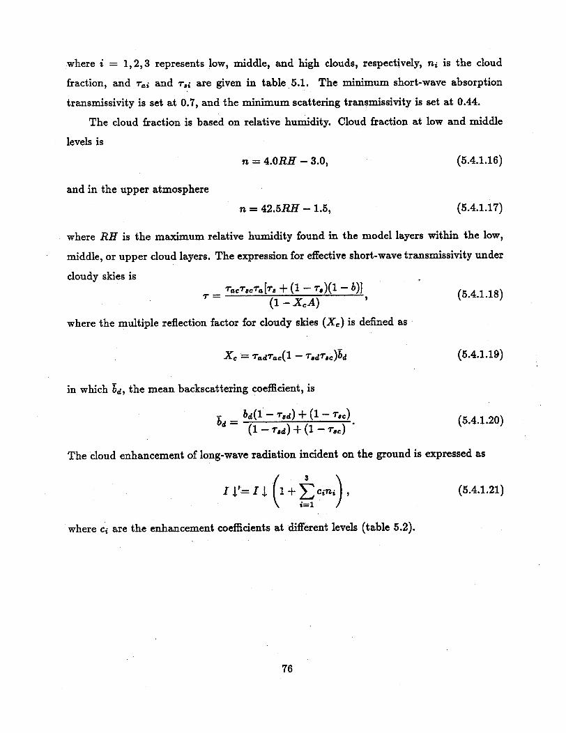
where i = 1,2,3 represents low, middle, and high clouds, respectively, ni is the cloud

fraction, and -ri and ri are given in table 5.1. The minimum short-wave absorption

transmissivity is set at 0.7, and the minimum scattering transmissivity is set at 0.44.

The cloud fraction is based on relative humidity. Cloud fraction at low and middle

levels is

n = 4.0RH - 3.0, (5.4.1.16)

and in the upper atmosphere

n = 42.5RH- 1.5, (5.4.1.17)

where RH is the maximum relative humidity found in the model layers within the low,

middle, or upper cloud layers. The expression for effective short-wave transmissivity under

cloudy skies isTr= crcT[T + (1 - b)] (5.4.1.18)

(1 - XA)

where the multiple reflection factor for cloudy skies (Xc) is defined as

Xc = 'adrac(1 - Tdr,c)bd (5.4.1.19)

in which bd, the mean backscattering coefficient, is

bd(1 - 8d) + (1 - 7c)bd re) + (1 ) (5.4.1.20)

(1 - 7,d) + (1 -- rc)

The cloud enhancement of long-wave radiation incident on the ground is expressed as

I '= 1 (+ cni , (5.4.1.21)

where ci are the enhancement coefficients at different levels (table 5.2).

76

Table 5.1 Cloud absorption and scattering transmissivities.

Cloud Level Absorption Scattering(tai) (.ti)

Low 0.80 0.48

Middle 0.85 0.60

High 0.98 0.80

Table 5.2 Enhancement coefficients ci on longwave radiation due to clouds.

Cloud Level Coefficient

Low 0.26

Middle 0.22

High 0.06

77

5.4.1.2 Heat Flow into the Substrate Hm

The transfer of heat due to molecular conduction is calculated from the equation

Hm, = KmCg(Tg - Tm), (5.4.1.22)

where Km is the heat transfer coefficient expressed as Km = 1.8fl, fl is the angular velocity

of the earth, and Tm is the temperature of the substrate, which is presently taken to be a

constant value equal to the mean surface-air temperature over the period of simulation. If

the model is used in a forecast mode rather than a research mode, Tm may be set equal

to the mean surface temperature of the previous day.

5.4.1.3 Sensible-Heat Flux H. and Surface Moisture Flux E.

These fluxes are computed in different ways, depending upon what PBL parameteri-

zation is used. Details will be described in the next sections.

5.4.2 Bulk-aerodynamic parameterization

The bulk-aerodynamic option of the PBL physics follows Deardorff (1972). It is a

very inexpensive choice. The surface-heat fluxes are given by

H. = paCpmCeCu( g- a)V, (5.4.2.1)

where pa and 0a are density and potential temperature at the lowest model layer, Co and

Cu are exchange coefficients (Deardorff 1972) defined as

C= C (1RiB) (5.4.2.2)

and

C =C CN R - ) (5.4.2.3)

for stable conditions (0 < RiB < .9Ric) and

C= (5.4.2.4)Cu= _ 25exp(.26, - .03,2)

and1

Ce= 1 1 1 (5.4.2.5)Oa N +s C, N

78

for the unstable case (RiB ' 0). Here CuN and CON are the neutral values for C, and Ce,

and are given by

CLN [f(-l Sf(O )+8 ] (5.4.2.6)LN\ [-Zo /

and

CON 0 .74k (.n 5) + 7.31 (5.4.2.7)

where Ric = 3.05, h is the depth of the lowest model layer, , is defined as

4 = logio(-RiB) - 3.5, (5.4.2.8)

and the velocity V is given by

V = (V 2 + V 2 ) 1/ 2. (5.4.2.9)

Ve is the wind-speed at the lowest model layer, and Vc is a convective velocity, which is

important under conditions of low mean wind-speed and is defined under unstable and

neutral conditions as

Vc = 2(8, - a),/2, (5.4.2.10)

while it is zero under stable conditions.

The surface moisture flux is

E, = paCeCuM(qv,(Tg) - qa)V, (5.4.2.11)

where M is the moisture availability parameter which varies from 1.0 for a wet surface to

0.0 for a surface with no potential for evaporation. The moisture availability is specified as

a function of land-use category (Appendix 4). The model results are often quite sensitive

to the value used for M.

The surface momentum flux is given by

r. = paCDV2 , (5.4.2.12)

where the drag coefficient CD is defined as

CD =CD+310 ( 800 (5.4.2.13)

79

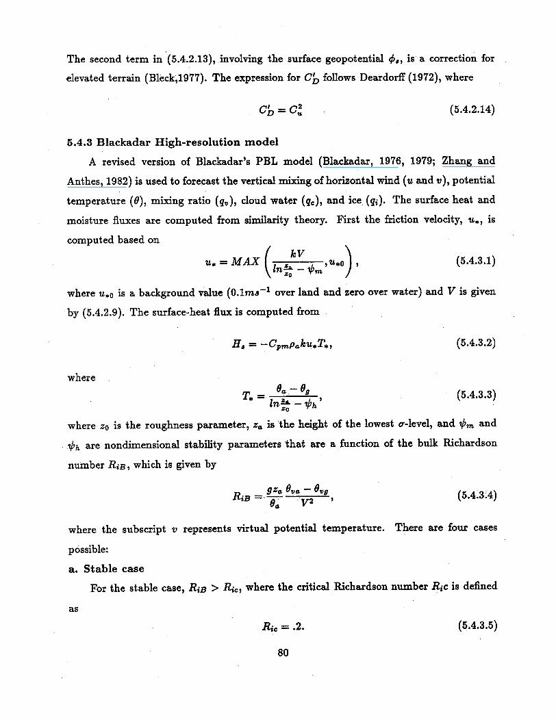
The second term in (5.4.2.13), involving the surface geopotential ,., is a correction for

elevated terrain (Bleck,1977). The expression for CD follows Deardorff (1972), where

CiC = C (5.4.2.14)

5.4.3 Blackadar High-resolution model

A revised version of Blackadar's PBL model (Blackadar, 1976, 1979; Zhang and

Anthes, 1982) is used to forecast the vertical mixing of horizontal wind (u and v), potential

temperature (6), mixing ratio (q,), cloud water (q,), and ice (qi). The surface heat and

moisture fluxes are computed from similarity theory. First the friction velocity, u., is

computed based on

u =oMAX , k , (5.4.3.1)

where u*o is a background value (O.lms-1 over land and zero over water) and V is given

by (5.4.2.9). The surface-heat flux is computed from

H, =-Cpmpaku*T*, (5.4.3.2)

where

T*= -- , (5.4.3.3)

where zo is the roughness parameter, Za is the height of the lowest ar-level, and bm and

Oh are nondimensional stability parameters that are a function of the bulk Richardson

number RiB, which is given by

gZ 1ae, - OvgRiB = 2 (5.4.3.4)

where the subscript v represents virtual potential temperature. There are four cases

possible:

a. Stable case

For the stable case, RIB > Ric, where the critical Richardson number Ric is defined

as

Ric=-*.2. (5.4.3.5)

80

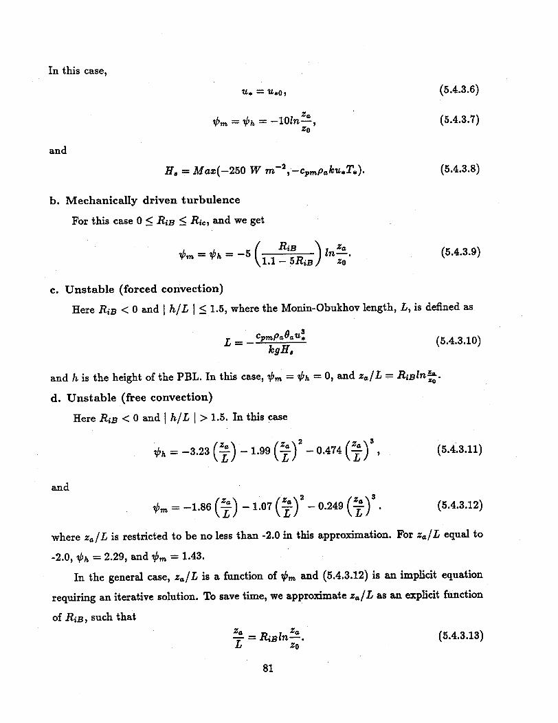
In this case,

u = u*0, (5.4.3.6)

,m =h =-101n-, (5.4.3.7)ZO

and

H, = Maz(-250 W m- 2 , -cppaku*T*). (5.4.3.8)

b. Mechanically driven turbulence

For this case 0 < RiB •< Ric, and we get

= h =-5 iRi n-. (5.4.3.9)( -5RiB) zo

c. Unstable (forced convection)

Here RIB < 0 and I hiL I < 1.5, where the Monin-Obukhov length, L, is defined as

L - cppOU* (5.4.3.10)kgH,

and h is the height of the PBL. In this case, bm = h = 0, and za/L = RiBlnZ^

d. Unstable (free convection)

Here RiB < 0 and i h/L I > 1.5. In this case

h= -3.23 () 1.99 (Z-) 0.474 ( 5)3, (5.4.3.11)

and

m=-1.86 ()- 1 *7( ) 2-0.249(L ) (5.4.3.12)

where za/L is restricted to be no less than -2.0 in this approximation. For za/L equal to

-2.0, Oh = 2.29, and Om = 1.43.

In the general case, za/L is a function of 1m and (5.4.3.12) is an implicit equation

requiring an iterative solution. To save time, we approximate za/L as an explicit function

of RiB, such that

X- = RBln-. (5.4.3.13)L ZO

81

The above scheme ensures continuity of 0/rm for all values of RiB. The formulation for the

surface moisture flux in the multi-layer case was derived from Carlson and Boland (1978),

where

E, = MpaI (q,,(T,) - qv), (5.4.3.14)

and

I-1= ku. [ (kIn . + z -) ,b (5.4.3.15)

The quantity zi is the depth of the molecular layer (0.01 m over land and zo over water)

and Ka is a background molecular diffusivity equal to 2.4 x 10-m 2 s 1.

Over land, the roughness length zx is specified as a function of land-use category

(Appendix 4). Over water, ZO is calculated as a function of friction velocity (Delsol et al.

1971) such that

ZO = 0.032u4/g + zoC, (5.4.3.16)

where zoc is a background value of 10-4m.

The Blackadar scheme considers two different PBL regimes, the nocturnal regime and

the free-convection regime. The first three cases (stable, mechanically driven turbulence,

and forced convection) are in the nocturnal regime, which is usually stable or at most

marginally unstable.

Nocturnal Regime

The first-order closure approach is used to predict model variables. The ground stress

is calculated from

r, = pu2, (5.4.3.17)

where u* is computed from (5.4.3.1). The components of T. in the z and y directions are

-== -Ur (5.4.3.18)

and

T =--T, (5.4.3.19)Va

where Va is the wind speed at the lowest model level. For surface layer variables, the

prognostic equations area90 -(Hi - Hs)89 at (=~if a D.m ) ~(5.4.3.20)Ot (paCpmzl)

82

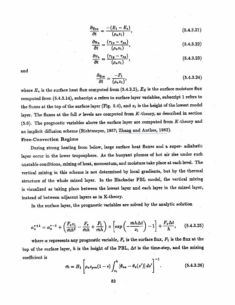
aqa (El - E.)t= (paz l) (5.4.3.21)

aUa (Tr1 - r a.) (5.4.3.22)

at (pazi)

Ova __ (r'l -- 'v)ata (piy -ty) (5.4.3.23)

and

Aqt -F l ) (5.4.3.24)t (paZi)'

where H, is the surface heat flux computed from (5.4.3.2), Es is the surface moisture flux

computed from (5.4.3.14), subscript a refers to surface layer variables, subscript 1 refers to

the fluxes at the top of the surface layer (Fig. 5.4), and zl is the height of the lowest model

layer. The fluxes at the full o levels are computed from K-theory, as described in section

(5.6). The prognostic variables above the surface layer are computed from K-theory and

an implicit diffusion scheme (Richtmeyer, 1957; Zhang and Anthes, 1982).

Free-Convection Regime

During strong heating from below, large surface heat fluxes and a super- adiabatic

layer occur in the lower troposphere. As the buoyant plumes of hot air rise under such

unstable conditions, mixing of heat, momentum, and moisture take place at each level. The

vertical mixing in this scheme is not determined by local gradients, but by the thermal

structure of the whole mixed layer. In the Blackadar PBL model, the vertical mixing

is visualized as taking place between the lowest layer and each layer in the mixed layer,

instead of between adjacent layers as in K-theory.

In the surface layer, the prognostic variables are solved by the analytic solution

T+laT 4 I-· , pFoz1 Fs F\ r (hAt FS Ata, - + (, h - m + -) x Iezp (-_ ) _-1 + ^ , (5.4.3.25)

Qa a in- \fmh2 m f-h h z 1 ) h

where a represents any prognostic variable, F. is the surface flux, F1 is the flux at the

top of the surface layer, h is the height of the PBL, At is the time-step, and the mixing

coefficient is

= H 1 [acpm(l - e) [va 0 (z)] dz] (5.4.3.26)z1

83

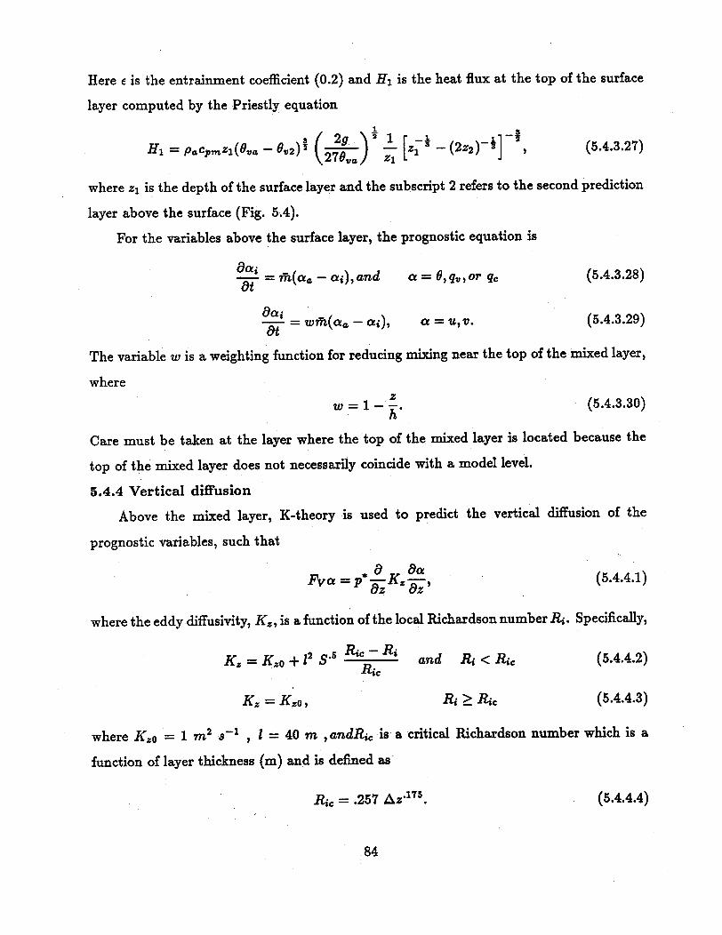
Here e is the entrainment coefficient (0.2) and H1 is the heat flux at the top of the surface

layer computed by the Priestly equation

H1 = paCpmZl(va - 2) (27 -) Z [z - (2Z 2 )-] j , (5.4.3.27)

where zl is the depth of the surface layer and the subscript 2 refers to the second prediction

layer above the surface (Fig. 5.4).

For the variables above the surface layer, the prognostic equation is

-a = m(a-o a), and a = , qv or qc (5.4.3.28)

at

w1= wfm(a - asi), a = uv. (5.4.3.29)

The variable w is a weighting function for reducing mixing near the top of the mixed layer,

where

w=l 1--. (5.4.3.30)h

Care must be taken at the layer where the top of the mixed layer is located because the

top of the mixed layer does not necessarily coincide with a model level.

5.4.4 Vertical diffusion

Above the mixed layer, K-theory is used to predict the vertical diffusion of the

prognostic variables, such that

Fva = a aaFva = p*| - K , (5.4.4.1)

where the eddy diffusivity, Kz, is a function of the local Richardson number Ri. Specifically,

K, = Ko +12 S' 5 R1 - and Ri < Ric (5.4.4.2)RtiC

K = Ko, Ri > Ric (5.4.4.3)

where Kzo = 1 m 2 s-1 , I = 40 m ,andRi, is a critical Richardson number which is a

function of layer thickness (m) and is defined as

Ric = .257 Az.175. (5.4.4.4)

84

Zs

Z41/2

h

24

Z3 1/2

Z3

Z211 2

22

Z1 1/2

Z1

Za. Za

F

a

F

a

F

a

F

a

F

a

Faova Ovg

9----

Figure 5.4 Illustration of vertical grid structure for high-resolution (Blackadar) model. The top ofthe surface layer is zj; Ovg and Ova are the virtual potential temperatures of the ground surface andlowest model level, respectively; P and N denote the positive and negative areas associated with aparcel of air originating at Za and rising to h, the top of the PBL.

85

According to (5.4.4.4), Ric varies from 0.58 for Az = 100 m to 0.86 for Az = 1000 m.

The Richardson number is

Ri = gS O (5.4.4.5)OS Oz

and S is

( ) + ( ) + 10 - 9 (5.4.4.6)

5.4.5 Moist vertical diffusion

There is an option with explicit moisture of including the effects of moisture on vertical

diffusion. Taking into account moist-adiabatic processes in cloudy air (Durran and Klemp

1982), (5.4.4.5) is modified to

R (1 ) [9 = (2+ t- (5.4.5.1)

where2

X - cRT 2 (5.4.5.2)

and

a RdT' (5.4.5.3)

and this modified value is used in (5.4.4.2) where the cloud amount exceeds 0.1 g

kg-.

86

5.5 Atmospheric radiation parameterization

The atmospheric radiation option in the model provides a longwave (infra-red) and

shortwave (visible) scheme that interact with the atmosphere, cloud and precipitation

fields, and with the surface (Dudhia 1989).

5.5.1 Longwave radiative scheme

Longwave absorption by water vapor, the primary clear-air absorber, is strongly

spectral in character, and the method employed is the commonly used broadband emissivity

method (see Stephens 1984). This involves using a precalculated emissivity function, e,

which represents the frequency-integrated absorption spectrum of water vapor, weighted

by a suitable envelope function. Rodgers (1967) gives an upward and downward emissivity

as a function of water vapor path, u, with a temperature correction term, where u includes

a pressure correction factor proportional to p0.86 . The form of the fitted function is

i=4

e(u) = Z(ai + Tbi)x, (5.5.1.1)i=-

where x = Inu and T is a u-weighted T - 250K. For u less than 10 g m - 2, the form is

i=4

e(u) = Z(ci + di)y', (5.5.1.2)i=l

where y = u 1/2 and ai, bi, ci and di are constants. In the tropics, e-type absorption is

an important additional component of the longwave absorption spectrum and is included

with a similar fourth-order polynomial in In (ue) to (5.5.1.1) from Stephens and Webster

(1979), where e is the partial pressure due to water vapor. Given the emissivity functions

from (5.5.1.1-2) (e, for upward flux and ed for downward flux), the upward and downward

fluxes at any model level are given by

F, = B(T)de, (5.5.1.3a)

Fd = ] B(T)ded, (5.5.1.4a)Jo

In (5.4.1.3a) the integration is performed downwards through the model layers. The

quantity de is calculated for each layer using the temperature (T) of the layer and the

87

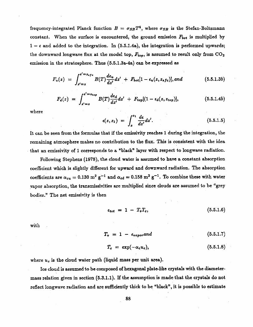
frequency-integrated Planck function B = CSBT 4 , where UaSB is the Stefan-Boltzmann

constant. When the surface is encountered, the ground emission Fbot is multiplied by

1 - e and added to the integration. In (5.5.1.4a), the integration is performed upwards;

the downward longwave flux at the model top, Ftop, is assumed to result only from CO2

emission in the stratosphere. Thus (5.5.1.3a-4a) can be expressed as

zL -Z'e s c deFd(z) = B(T)j dz' + Fbot[l- ,(z,z.fc)],and (5.5.1.3b)

ZJ'= o dz

Fd(z) = X B(T) dz' + Ftop[(l-Ed (Z Ztop)] (5.5.1.4b)

wherezL de

e(zz) = J ,dz. (5.5.1.5)

It can be seen from the formulas that if the emissivity reaches 1 during the integration, the

remaining atmosphere makes no contribution to the flux. This is consistent with the idea

that an emissivity of 1 corresponds to a "black" layer with respect to longwave radiation.

Following Stephens (1978), the cloud water is assumed to have a constant absorption

coefficient which is slightly different for upward and downward radiation. The absorption

coefficients are acu = 0.130 m 2 g- 1 and acd = 0.158 m 2 g-1. To combine these with water

vapor absorption, the transmissivities are multiplied since clouds are assumed to be "grey

bodies." The net emissivity is then

tot = 1 - Tv,T, (5.5.1.6)

with

Tv = 1 - vapraand (5.5.1.7)

TC = exp(-~cc), (5.5.1.8)

where uc is the cloud water path (liquid mass per unit area).

Ice cloud is assumed to be composed of hexagonal plate-like crystals with the diameter-

mass relation given in section (5.3.1.1). If the assumption is made that the crystals do not

reflect longwave radiation and are sufficiently thick to be "black", it is possible to estimate

88

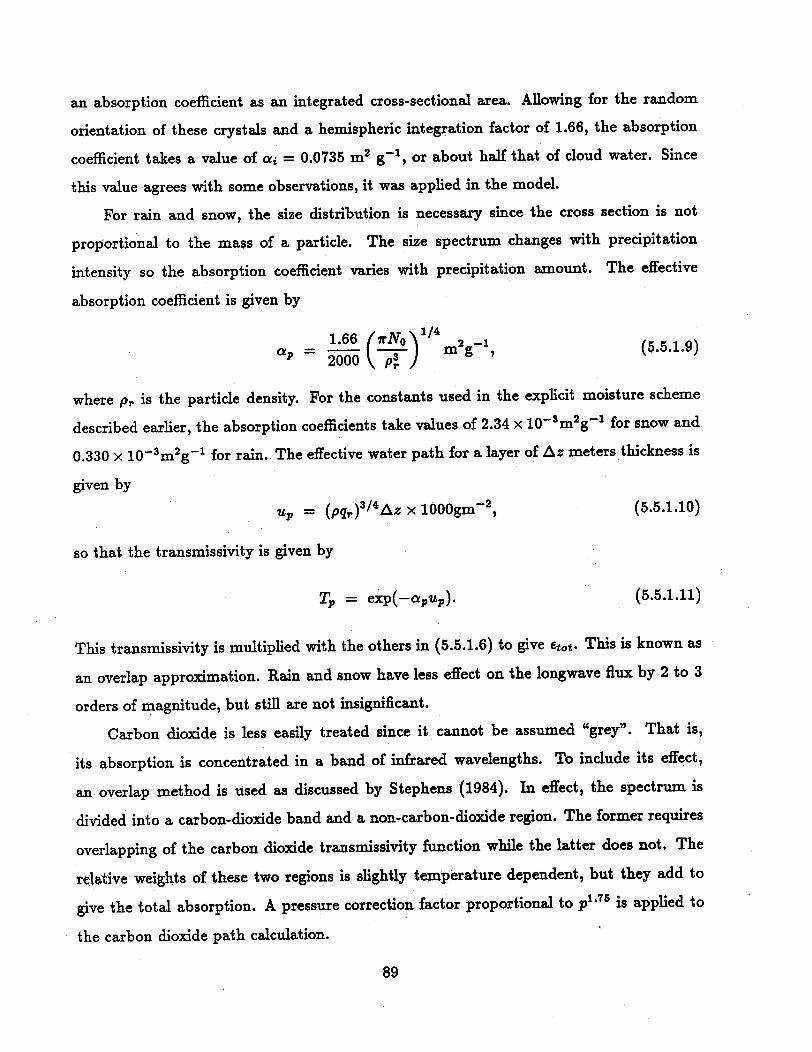
an absorption coefficient as an integrated cross-sectional area. Allowing for the random

orientation of these crystals and a hemispheric integration factor of 1.66, the absorption

coefficient takes a value of ai = 0.0735 m2 g'l, or about half that of cloud water. Since

this value agrees with some observations, it was applied in the model.

For rain and snow, the size distribution is necessary since the cross section is not

proportional to the mass of a particle. The size spectrum changes with precipitation

intensity so the absorption coefficient varies with precipitation amount. The effective

absorption coefficient is given by

1.66 1TrNo 1/4 2 -519)p = 2000 (rg (5.5.1.9)

where pr is the particle density. For the constants used in the explicit moisture scheme

described earlier, the absorption coefficients take values of 2.34 x 10-Sm2 g- 1 for snow and

0.330 x 10-3m 2g- 1 for rain. The effective water path for a layer of Az meters thickness is

given by

up = (pqr)s/4z x 1000gm- 2 , (5.5.1.10)

so that the transmissivity is given by

Tp = exp(-apup). (5.5.1.11)

This transmissivity is multiplied with the others in (5.5.1.6) to give etot. This is known as

an overlap approximation. Rain and snow have less effect on the longwave flux by 2 to 3

orders of magnitude, but still are not insignificant.

Carbon dioxide is less easily treated since it cannot be assumed "grey". That is,

its absorption is concentrated in a band of infrared wavelengths. To include its effect,

an overlap method is used as discussed by Stephens (1984). In effect, the spectrum is

divided into a carbon-dioxide band and a non-carbon-dioxide region. The former requires

overlapping of the carbon dioxide transmissivity function while the latter does not. The

rlative weights of these two regions is slightly temperature dependent, but they add to

give the total absorption. A pressure correction factor proportional to p1. 75 is applied to

the carbon dioxide path calculation.

89

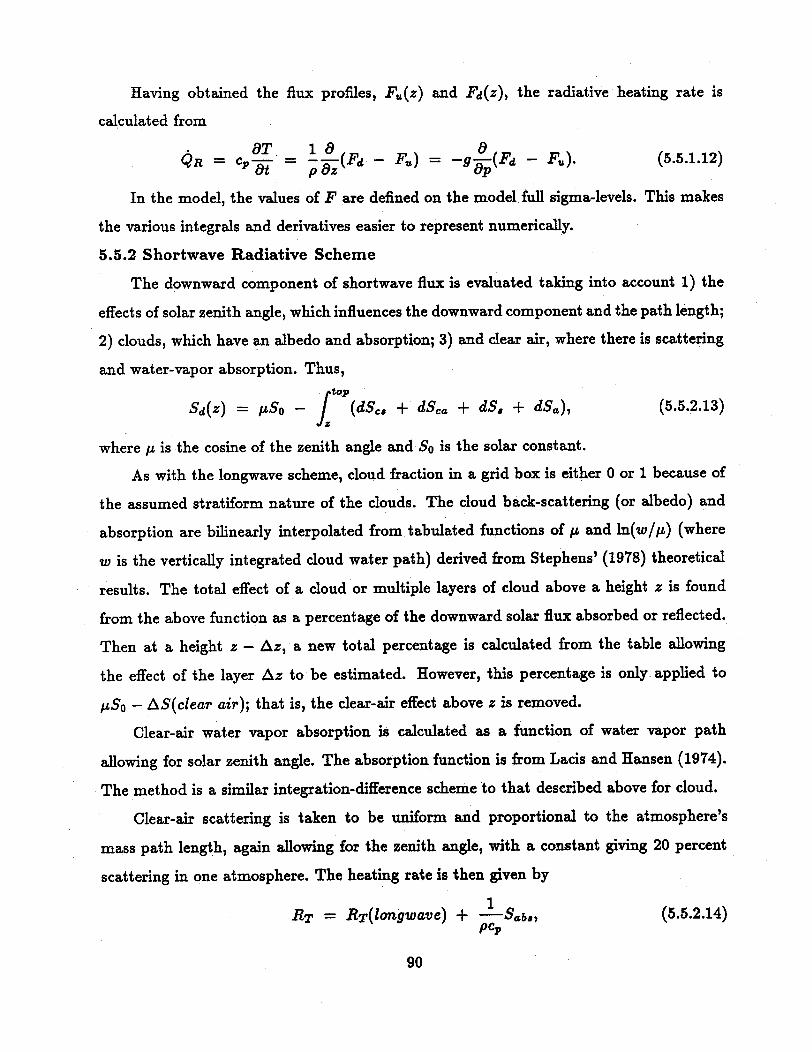
Having obtained the flux profiles, Fu(z) and Fd(z), the radiative heating rate is

calculated from

_T 18 8QR = C a' = - (Fd - Fu) = -g (Fd - F. (5.5.1.12)

In the model, the values of F are defined on the model full sigma-levels. This makes

the various integrals and derivatives easier to represent numerically.

5.5.2 Shortwave Radiative Scheme

The downward component of shortwave flux is evaluated taking into account 1) the

effects of solar zenith angle, which influences the downward component and the path length;

2) clouds, which have an albedo and absorption; 3) and clear air, where there is scattering

and water-vapor absorption. Thus,t/op

Sd(Z) = So - j (dSc, + dSca + dS, + dSa), (5.5.2.13)Jz;

where 1p is the cosine of the zenith angle and So is the solar constant.

As with the longwave scheme, cloud fraction in a grid box is either 0 or 1 because of

the assumed stratiform nature of the clouds. The cloud back-scattering (or albedo) and

absorption are bilinearly interpolated from tabulated functions of p and ln(w/p) (where

w is the vertically integrated cloud water path) derived from Stephens' (1978) theoretical

results. The total effect of a cloud or multiple layers of cloud above a height z is found

from the above function as a percentage of the downward solar flux absorbed or reflected.

Then at a height z - Az, a new total percentage is calculated from the table allowing

the effect of the layer Az to be estimated. However, this percentage is only applied to

pISo - AS(clear air); that is, the clear-air effect above z is removed.

Clear-air water vapor absorption is calculated as a function of water vapor path

allowing for solar zenith angle. The absorption function is from Lacis and Hansen (1974).

The method is a similar integration-difference scheme to that described above for cloud.

Clear-air scattering is taken to be uniform and proportional to the atmosphere's

mass path length, again allowing for the zenith angle, with a constant giving 20 percent

scattering in one atmosphere. The heating rate is then given by

1RT = RT(longwave) + Sabs, (5.5.2.14)

PCp

90

where Sabs is defined from the absorption part of the Sd integral given in (5.5.2.13), since

only cloud and clear-air absorption contribute to solar heating.

The solar and infrared fluxes at the surface, calculated from the atmospheric radiative

schemes, are use in the energy budget of the land surface.

91

Appendix 1. Glossary of Symbols

a Fraction of convective cloud cover; also constant used in cloud

microphysics

ABE Available buoyant energy

AT The forcing terms of the thermodynamic equation that vary on the

time-scale of the Rossby-waves

AU, Ad, Atot Cloud Work Function for updraft, downdraft, and all of model cloud

Av The forcing terms of the v-momentum equation that vary on the time-

scale of the Rossby-waves

Av The forcing terms of the u-momentum equation that vary on the time-

scale of the Rossby-waves

A' Parameter for heterogeneous freezing (K- 1 )

A Antidiffusive flux

b Backscattering coefficient; also fraction of total water vapor conver-

gence used to moisten grid column (section 5.3.2.1); also constant

(0.8) used in cloud microphysics computation

B Planck function

Bu Acceleration due to buoyancy

B' Parameter for heterogeneous freezing (m-s - 1)

Co Rainfall conversion parameter (section 5.3.2.2)

92

Cm Constant used in computation of Dm

ci Coefficients used in calculation of cloud effect on downward longwave

radiation (Table 5.2)

Cp Specific heat at constant pressure for dry air

Cpm Specific heat at constant pressure for moist air

c* Net condensation rate averaged over grid volume

C* Net condensation rate in cumulus cloud (section 5.3.2.1)

C Constant (2. m s - 1 K - 1/ 2 ) used in computing convective velocity

Cg Thermal capacity of slab per unit area (J m - 2 K- 1)

C, Heat capacity per unit volume (J m - 3 K - 1)

Ce Surface exchange coefficient for heat

CU Surface exchange coefficient for momentum; also total condensate in

updraft (section 5.3.2.2)

CD Surface drag coefficient

CD Component of surface-drag coefficient

CN Value of surface momentum exchange coefficient under neutral

stability conditions

93

CON

D

Df

D?, Dd, Dtot

Di

D2a

Dm

e

e., esi, eaw

E

E,

f

fi, f2

Value of surface heat exchange coefficient under neutral stability

conditions

Mass divergence (hydrostatic split-explicit scheme); also horizontal

deformation (section 5.1)

Diffusivity of water vapor in air

Updraft, downdraft, and total cloud kinetic energy dissipation

Distance between an observation and a given grid point (section 4)

Diameter of ice crystal (m)

Diffusion and PBL tendencies for variable a

Modified distance between an observation and a given grid point

(section 4)

Horizontal Coriolis parameter (s - 1)

Saturation vapor pressure, over ice, over water (cb)

Efficiency of collection of cloud by precipitation; also vertical flux of

water vapor

Flux of water vapor from surface into atmosphere

Coriolis parameter

Ventilation coefficients for rain or snow

94

F Larger-scale forcing (section 5.3.2.2 and 5.3.2.3); also function of

distance from lateral boundary (section 2.6.2)

FH, FL Flux from high-order and low-order advective scheme

Fbot, Ftop Longwave radiative flux at bottom, top of model atmosphere (W m- 2 )

Fd, Fu Downward, upward longwave radiative flux (W m - 2 )

FHa Term representing contribution of horizontal diffusion of a variable a

to the temporal rate of change of a

Fva Term representing contribution of vertical diffusion of a variable a to

the temporal rate of change of a

F, Flux of dry static energy (section 5.3.2.2); also Surface flux of heat,

moisture or momentum

Fq Flux of water vapor (section 5.3.2.2)

Ft Flux of suspended cloud liquid water (section 5.3.2.2)

Fr Deceleration

F1,F 2 Amplitude factors used in computing lateral boundary conditions

(section 2.6.2)

g Acceleration of gravity (9.8 m s - 2 )

h Moist static energy; also height of planetary boundary layer (m)

ho Local hour angle of sun

95

h, h, hu, hdh* Moist static energy in environment, cloud, updraft, downdraft, and

saturation value in environment

H Vertical flux of sensible heat (W m - 2)

Hm Heat flux into substrate (W m - 2 )

Ha Sensible heat flux from surface into atmosphere (W m - 2 )

I Function of static stability and surface friction velocity; also horizontal

grid-index in y-direction

IMAX Maximum value of grid-index in y-direction

I, Net longwave iradiance at surface (wm- 2 )

I t Outgoing longwave radiation from surface (W m - 2)

I 1 Downward longwave radiation absorbed at surface (W m - 2) under

clear skies

I 1' Downward longwave radiation absorbed at surface (W m - 2) in

presence of clouds

I1 Normalized condensate in updraft (section 5.3.2.2)

I2 Normalized evaporate in updraft (section 5.3.2.2)

J Horizontal grid index in a-direction

JMAX Maximum value of grid index in x-direction

96

k

k

k'

K

KH.KHl

Km

KMAX

Kz

Kzo

KEu, KEd, KEtot

L

Lm

Dimensionless a-wavenumber for upper radiative scheme; also von

Karman constant (0.4)

Dimensionless effective ma-wavenumber for upper radiative scheme

Constant used in formula for computing autoconversion of cloud drops

to rain drops

Total horizontal wavenmumber (m ' l ) also Kernels

Background molecular diffusivity (2.4 x 10- 5m 2 s-1); also thermal

conductivity of air ( J m - 1 s- 1 K- 1 )

Horizontal eddy diffusivity (m 2 s - 1)

Coefficient used in fourth-order diffusion (s - 1)

Background value of horizontal eddy diffusivity (m 2 s - 1)

Coefficient of heat transfer from ground into substrate (s - 1)

Maximum value of index in vertical direction

Coefficient of vertical diffusivity (m 2 s - )

Background value of coefficient of vertical diffusivity (m 2 s - 1)

Kinetic energy for updraft, downdraft, and all of model cloud

Hydrostatic term due to liquid water loading; also Monin-Obukhov

length

Latent heat of fusion (0.35 x106 J kg- 1)

97

Ls Latent heat of sublimation (2.85 x106 J kg - 1)

/Lv Latent heat of condensation (2.5 xl06 J kg-1)

I Dimensionless y-wavenumber for upper radiative scheme; also vertical

mixing length

I Dimensionless effective y-wavenumber for upper radiative scheme

Mi Mass of ice crystal (kg)

Mmaz Maximum mass of ice crystal (kg)

Mo Initial mass of ice crystal (kg)

m Mass flux (updraft and downdraft) in convective parameterization

cloud (5.3.2.2); also map scale factor

f'm MMixing coefficient used in free-convective regime of high-resolution

PBL model

mb Cloud base mass flux (section 5.3.2.2)

mO Downdraft base mass flux (section 5.3.2.2)

mu Updraft mass flux in convective parameterization cloud (5.3.2.2)

md Downdraft mass flux in convective parameterization cloud (5.3.2.2)

M Surface moisture availability

98

Vertical integral of horizontal convergence of water vapor

n Fraction of cloud

no Cloud microphysics parameter

nc Number concentration of ice crystals (kg- 1)

N Brunt-Vaisla frequency (s- 1)

Nc Number concentration of cloud droplets per unit volume (1010 m - 3 )

Nh Nondimensional function for vertical profile of convective heating

Nm Nondimensional function for vertical profile of convective moistening

N o Cloud microphysics parameter (8 x 106 m - 4 for rain 2 x 107 m - 4 for

snow)

p Pressure (cb)

Pb Pressure (cb) at convective cloud base

pa Surface pressure (cb)

pt Pressure (cb) at top of model

pU Pressure (cb) at top of convective cloud

PLCL Pressure (cb) at lifting condensation level

99

P P - Pt (cb)

Pd Dot-point p* (cb)

Po Reference-state pressure

p' Perturbation pressure (Pa)

Pressure value representing the free atmosphere, where terrain

influences are small (in FDDA)

~~~~p ~ Fourier transform of p' for upper radiative boundary condition

PCON Condensation of water vapor or evaporation of cloud drops (kg kg- 1

s- 1 )

PRA Accretion of cloud drops by rain drops (kg kg-l s - 1)

PRC Autoconversion of cloud drops to rain drops (kg kg - l s.~)

PRE Evaporation of rain drops (kg kg-l s - 1)

PCI Heterogeneous freezing of cloud water (kg kg s - 1)

PID Deposition of vapor onto ice crystals (kg kg s - 1)

PII Initiation of ice crystals (kg kg s - 1)

PMF Melting/freezing of cloud and precipitation due to advection (kg kg

S-1)

100

PRM

PSM

>, qu qd>, q

qco

Melting of falling precipitation (kg kg s - 1)

Melting of falling snow (kg kg s - 1)

Water vapor mixing ratio in environment, updraft, downdraft, and

saturation value in environment

Mixing ratio of cloud water; also water vapor mixing ratio in cloud

(section 5.3.2.2)

Critical value of mixing ratio of cloud water

Mixing ratio of rain water

Suspended liquid water vapor mixing ratio inside updraft

Mixing ratio of water vapor

Mixing ratio of water vapor in cumulus cloud

Saturation mixing ratio of water vapor

Diabatic heating rate per unit mass (J kg- 1 s - 1)

Net short wave irradiance at the surface (W m - 2 )

Rainfall (convective-scale sink of cloud water, 5.3.2.2); also ideal gas

constant for dry air (287 J kg- 1 K - 1)

Relative humidity

Richardson number

101

qv

Q

Qs

R

RH

Ri

Rn Net radiation

RiB Bulk Richardson number

Ric Critical value of bulk Richardson number; also critical value of

Richardson number

Rv Gas constant for water vapor (461.5 J kg- l K - 1)

RT Radiative heating rate (K s - 1)

r Radius of convective parameterization cloud (sections 5.3.2.2)

S Supersaturation; also source or sink term (section 5.3.2.2); also square

of the vertical wind shear

Sc Schmidt number

SO Solar constant (1395.6 W m-2 )

Su Source or sink term in updraft (section 5.3.2.2)

Sd Downward solar flux (W m-2 ); also source or sink term in downdraft

(section 5.3.2.2)

Si Supersaturation over ice

s Dry static energy

t Time (s)

102

T Temperature (K)

TC Longwave transmissivity due to cloud

Td Dewpoint temperature (K)

Tg Temperature (K) of ground

Tp Longwave transmissivity due to precipitation

Tv Virtual temperature (K); also longwave transmissivity due to vapor

T. Surface friction temperature (K)

To Reference-state temperature (K)

T' Perturbation temperature (K)

u Component of wind velocity in eastward direction (m s- 1); also water

vapor path (g m 2 )

us Surface friction velocity (m s - 1)

uc, Up Liquid water path for cloud, precipitation (g m - 2 )

v Component of wind velocity in northward direction (m s - 1)

vt Mass weighted mean terminal velocity of rain drops (m s-1 )

V Fall speed of a precipitation particle (m s - 1); also modified horizontal

wind velocity in PBL

103

V Horizontal wind vector

Va Horizontal windspeed at lowest model layer

Vc Convective PBL velocity(m s - 1)

Vqf Divergence of vertical eddy flux of water vapor due to convective

clouds

w Vertical velocity (m s- 1); also weight function for reducing mixing

near top of mixed layer

Wn Weight function for blending model tendencies and large-scale

tendencies near lateral boundaries (section 2.6.1)

Wp Precipitable water (cm)

Wu Vertical velocity in updraft

w Fourier transform of w

:x Horizontal grid coordinate increasing generally eastward

X Horizontal coordinate on earth surface increasing generally eastward

Xc Multiple-reflection factor in cloudy air

Xd Distance vector

XR Multiple-reflection factor in clear air

104

y Horizontal grid coordinate increasing generally northward

Y Horizontal coordinate on earth surface increasing generally northward

z Height above surface (m)

Za Height of lowest layer in model (m)

Zb Height of updraft originating level(section 5.3.2.2) (m)

ZO Height of downdraft originating level(section 5.3.2.2); also surface

roughness length(m)

ZoC Background value of surface roughness length over water (104m)

zl Depth of molecular layer

ZLCL Height of lifting condensation level (m)

ZT Height of updraft top (section 5.3.2.2)

a Coefficient array for upper radiative boundary condition (m s- 1

Pa, 1 ); also any thermodynamic variable (section 5.3.2.2)

& Any thermodynamic variable in environment

au Any thermodynamic variable in updraft

ad Any thermodynamic variable in downdraft

ac, ap Longwave absorption coefficients for cloud, precipitation (m 2 g-)

105

,l5Pf~ tParameter in sound-wave temporal differencing; also precipitation

efficiency parameter in section 5.3.2.2

r Gamma function

rd Dry adiabatic lapse rate (K m - 1)

rdp Dewpoint adiabatic lapse rate (K m 1)

7 Ratio of heat capacities (cp/cv) for dry air

S Solar declination

sM Supersaturation or undersaturation

Ap Vertical grid size (Pa)

As Horizontal grid length (m)

At Time step (s)

At' Short time step for rain fall term (s)

Ax Horizontal grid length (m)

Az Thickness of vertical layer (m)

Aa Thickness of model a levels

106

Aac Critical value of convective cloud depth

Ar Short time step for sound waves (s)

V2 Horizontal Laplacian on a-surfaces

V4 Fourth order diffusion operator on a-surfaces

e Parameter relating updraft and downdraft mass flux (section 5.3.2.2);

also small value; also entrainment coefficient used in high resolution

PBL-model (0.2)

ea Atmospheric emissivity

Qeg~~ ~ Emissivity of ground

e,, ed Atmospheric longwave emissivity

ld Normalized mass flux for downdraft (section 5.3.2.2)

nlu Normalized mass flux for updraft (section 5.3.2.2)

6 Potential temperature (K); also angle between y-axis and northfor

full Coriolis force

aa Potential temperature (K) at lowest layer in model

0Bs@~ ~Potential temperature (K) of ground surface

Ge Equivalent potential temperature (K)

107

Saturation equivalent potential temperature (K)

Virtual potential temperature (K)

Longitude; also cloud type (section 5.3.2.2); also thermal conductivity

(J m - 1 s-l K-1 ); also parameter in raindrop distribution (m - 1)

Dynamic viscosity of air (kg m - 1 s- 1); also solar zenith angle ; also

total net fractional entrainment rate (section 5.3.2.2); also constant

in smoother (section 3.3)

Total net fractional entrainment rate for updraft (section 5.3.2.2)

Gross fractional entrainment rate for updraft (section 5.3.2.2)

Gross fractional detrainment rate for updraft (section 5.3.2.2)

Coefficient for Asselin time filter; also for spatial smoother

Exner function

Density of air (kg m - 3 )

Particle density (kg m - 3 )

Density in updraft

Density of water (kg m - 3)

Reference-state density (kg m - 3 )

108

A

ALu

ilue

AIud

v

7r

p

Pr

Pu

Pwu

Po

0es

oV

p' . Perturbation density (kg m - 3)

a Nondimensional vertical coordinate of model

a' Dummy variable of integration

&~a~ ~~Vertical velocity in a-coordinates (s - 1)

&c Vertical velocity of convective cloud in a-coordinates (s - 1 )

aSB Stefan-Boltzmann constant (5.67051 x 10- 8 J m - 2 K - 4 s - 1 )

r Half-period of time window of influence of an observation (section 4);

also short-wave transmissivity

Ir Short-wave transmissivity obtained from lookup table

a Clear air absorption transmissivity

a'c Cloudy air absorption transmissivity

7r Clear air scattering transmissivity; also surface stress

7-C Cloudy air scattering transmissivity

Geopotential; also latitude; also scalar variable in advection equation

(f Surface geopotential

109

Symbol denoting low-order, monotonic solution to advection equation

x Diffusivity of vapor in air (m 2 s - 1); also thermal inertia

QP Solar zenith angle; also function of bulk Richardson number

I'm Nondimensional stability parameter for momentum

Ah Nondimensional stability parameter for heat and water vapor

w Vertical velocity in pressure coordinates (cb s-1)

oc Vertical velocity of convective cloud in pressure coordinates (cb s - 1 )

/1 Angular velocity of earth (7.2722 x 10-5 s-l)

110

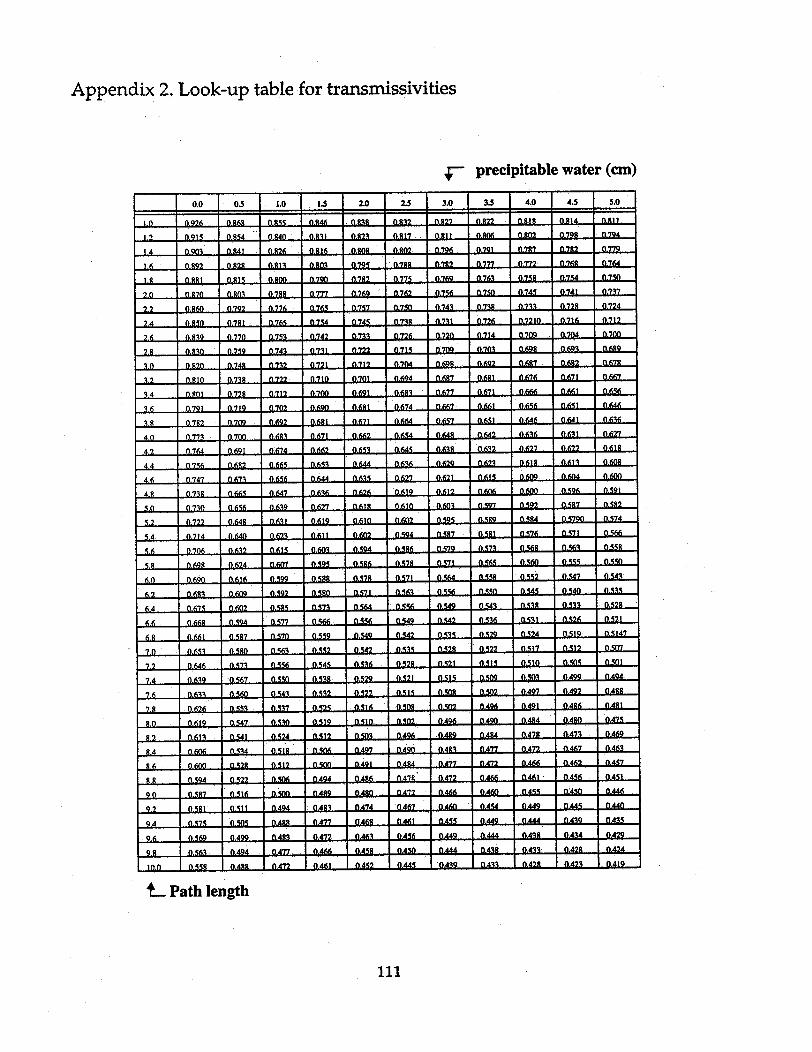
Appendix 2. Look-up table for transmissivities

~" precipitable water (cm)

0.0 0.5 1.0 .5 20 25 3.0 3.5 4.0 4.5 5.0

10 0.926 0,868 0.855 0s 46 .08o38 .832 0.827 0.,S22 o- I - o.R14

1.2 0.915 0.854 0.40 0.831 0.823 817 0.R11 0.806-- JLS2- 2- - -JL224

1.4 0.903 0Q.841 0.826 08R16 0.808 0802 0.796-1 0.726 0.8{Y2- 0.7928 224

1.6 08-92 08.28 0n.8R13 0803m 0.795- 07R 0 .79LZ2- n-0222- J7Z22- J0ff7 - 02i4

1. , 08 0.89 1 5 0.860 0.790 0.782 0.775- %flj0i2 6 0254- 0250

2.0 0.870 0.03 0.788 0.777 0.769 Ol0 2562 0.76 0.7502 0245 02741. 0. 22

2.2 0, 6 0.792 0.776 0.765 0.7957 0.750 0.742 Q.77'/ 0.7922

2.4 0.850 0..781- 0.765 0 0, 7 45 0.774 0,745 -22f71- 0.1726 0.716 -5212

2.6 0.839 0.770 0 .753 Q.77 7 0.769 0.74 2 0.730 0. 7 0214 009 0.704

2. , 0.860 0.759 0.743 0. 71 071 722 0715 0.7094 0.73Z03 -62S 03693- 0L629

3.0 0O.8R2O. 0748 0.732 0721 0.712-- 0.704 JQ.69S-- Jf2 - OAff7 0J,6i2-- 0O627 -

3.2 0.810 0.-738 0.722 0.710t 0.701 0Q.694 0.6M7 fi 3.7g 0.636 0.2g6 i 0.62 6

3.4 080R1 0.728 0.712 0.700 0691- 0.683-- n-677-- 0,671 0fii666-J(.if1-- -. 65fi-

.46 0.791 0.719 0.702 0.690 4 0, 8 I 0.674 0.6673 0 -66 !O5 5 0651 .

3. 0.7S2 0.709 0.692 061 0/671 0.1664 .6 0651 0641

420 0.773 0.770 0.673 0.71 0.662 0.7654 0.649 0.7142 0636 0 .631 0627

4.2 0.764 '0.69 6 0,74 0662 0.6531 0 645 0.7 0 2 627 2 &I

4.4 0.756 0.682 0.665 0 n653 0.644 0.636 0.6292 . 22 0.623 0.61-9

46 0.2747 0.673 0.656 0.64 0.650.7 0.621698064506562 0609 0

489 0-738 0(.665 0n6.647 Q.636 0,626 0.0619 0.612 0606 0.600 0.5962 .

5.0 0.730 0.656 -. 0.639 0.627 0618 .61O 0.603-- 0.597- JOL592- J 57 L 5 92- SS2-

5.2 0.722 0Q.648 0.631 0 619 0(.610 0.602 0.595-- JL5f92--J a -- O.?790 J -

5.4 0.714 0640 0.623 0.611 0602 0.62 594 0-JS7- LSJ-- - 05 71-- .5

68

5.6 0.706 0.632, 0,615 0.603 0.594 0Q.586- Q.579- 0L5227 S6-1 0 . 676 0.567 .67

5 0.698 01 0.624 607 0 .70595 0.586 0.578 0.577 0.565 0.5666IL55 -J55 -

60 093.69 0.7 599 105 0.578 0.571 0,564 .655 0.552 0.642 0.546-6

6.2 0 683 0-609 0 Q592 0n.580 0.571 0.563 051.661 5 -0 0.6456 -0.5146 - L5

6.4 0.675 2 0 .602 09 5 0.6 7 1 60.556.0573 0564 0556-0.63 2

6.6 0.668 0.594 0.577 0.566. 0.556 0.5496 0.542-0565 05210.

6. ,661 0.87 0 570 0.5 6059 67529 0L24 0J512 0,5147

TO Q.653 Q-5RO 0,563 0,552 0-542 0-535 0,520,642 00.63 6 00.631 0.62

7.2 0.646 0.6 1 0.5763 4 .4620.553 6 4 528 21 621 15 552 510 5--AS 501

-7'.4 0.639 0.567 0.550 0538 0.529 0.521 _ L515- CLSE 0.602 7 0.422- 0.61424

7.6 0.563 0.6532 0.522 0:63 0.515 0.20 0.649

789 0.626 0.553 0,537 0.525 0,516 0.508 0.502- 0.49623 0.691 0.496 0 .64

4. , 0.679 5 0.67 0.530 0.519 0.510 0.562 0.496 04906 4S4 1Z

8.2 0.613 0.541 0.524 0.512 05.69 A .6 9 44 00.6900--473

4 0 660.66 06534 0,55 1 0.563 0.09479 0-4 L4621

8.6 0.600 0 528 0.-512 0.500 0.491 -0.484 0.477-- Q22- f~ff- -0. 4626. 0.515.0 0.594 0.522 0.506 0.494 0.48 0.6418 0.403

0.497 0,49 .70 512

9.0 0.587 0.6 0.5 1 0.419 0.640 0.402 0.5455905450- B.f

9.2 0.581 0,511 0.494 048R3 0,474 0.... -467- 0.460 J -0.42 0.449 5 0,440

9 ,4 0.575 0.540 0 .6 2 8 04 77 0.468 0.42 444 A39 0.25

9~~~~~~~~~~~~~~~~~~~~~~~~~.76 0.57 4296

9.6 0.569 0.499 0.413 0.472 0.463 056 0.449 0, 4 2 2

9.8 0.563 0.494 0.477 0,466 0.AM 58-0.644 0 -.55 0.55 0.547-22- 429'

6,20.60 30.6558 0.48 042 0.461 0.452 .J456 3 42- 22 42-042.5412

Fma (.55R 0.449 . 0 .4_ 0.426 1 0.426 0.219

Path l.6eng7t.7h059 .4 052 .

111

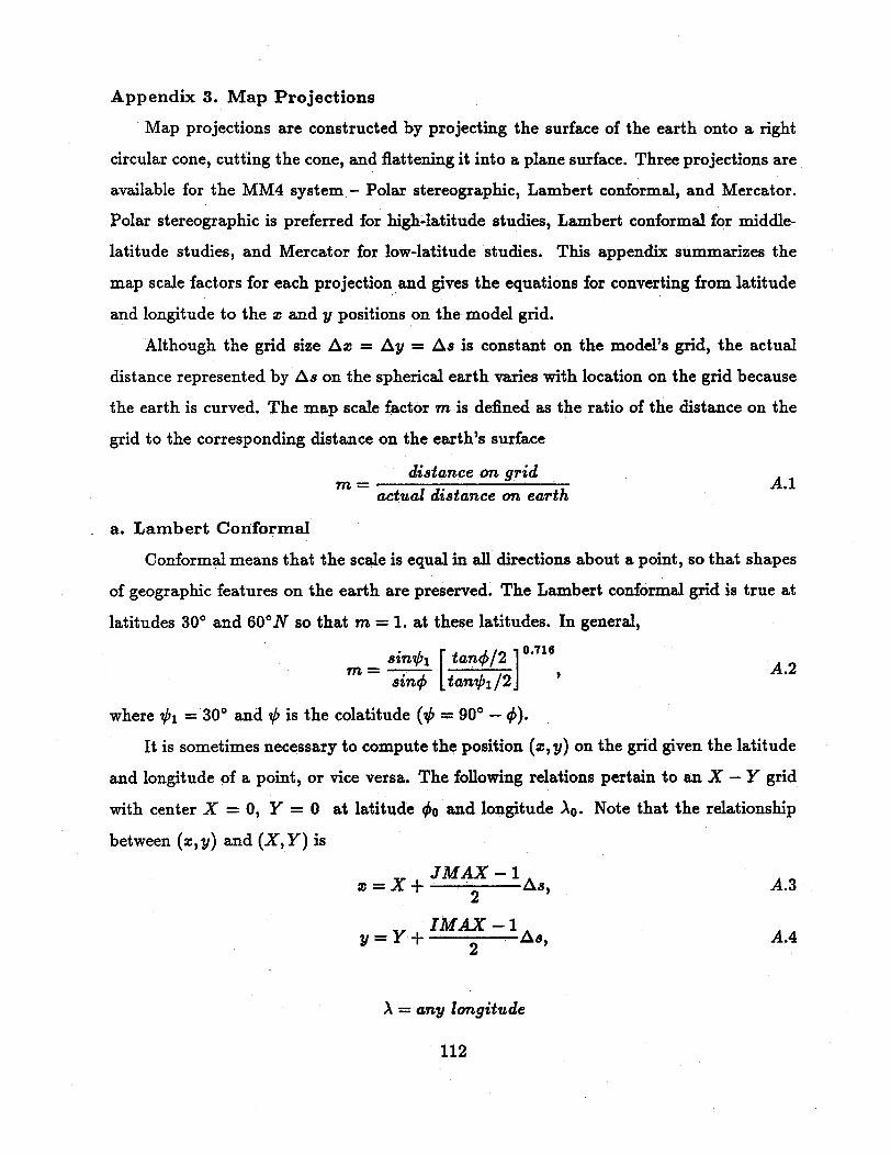
Appendix 3. Map Projections

Map projections are constructed by projecting the surface of the earth onto a right

circular cone, cutting the cone, and flattening it into a plane surface. Three projections are

available for the MM4 system - Polar stereographic, Lambert conformal, and Mercator.

Polar stereographic is preferred for high-latitude studies, Lambert conformal for middle-

latitude studies, and Mercator for low-latitude studies. This appendix summarizes the

map scale factors for each projection and gives the equations for converting from latitude

and longitude to the x and y positions on the model grid.

Although the grid size Amc = Ay = As is constant on the model's grid, the actual

distance represented by As on the spherical earth varies with location on the grid because

the earth is curved. The map scale factor m is defined as the ratio of the distance on the

grid to the corresponding distance on the earth's surface

distance on gridactual distance on earth A

a. Lambert Conformal

Conformal means that the scale is equal in all directions about a point, so that shapes

of geographic features on the earth are preserved. The Lambert conformal grid is true at

latitudes 30° and 60°N so that m = 1. at these latitudes. In general,

sinel [ tan_/2 ] 0.716 Asinf tano', /2.,

where b1 = 30° and ,b is the colatitude (, = 90° - ).

It is sometimes necessary to compute the position (a, y) on the grid given the latitude

and longitude of a point, or vice versa. The following relations pertain to an X - Y grid

with center X = 0, Y = 0 at latitude To and longitude Ao. Note that the relationship

between (x, y) and (X,Y) is

JMAX-1a = X + 2.. .. As, A.3

2

IMAX- 1y = Y + . As, A.4

2

A= any longitude

112

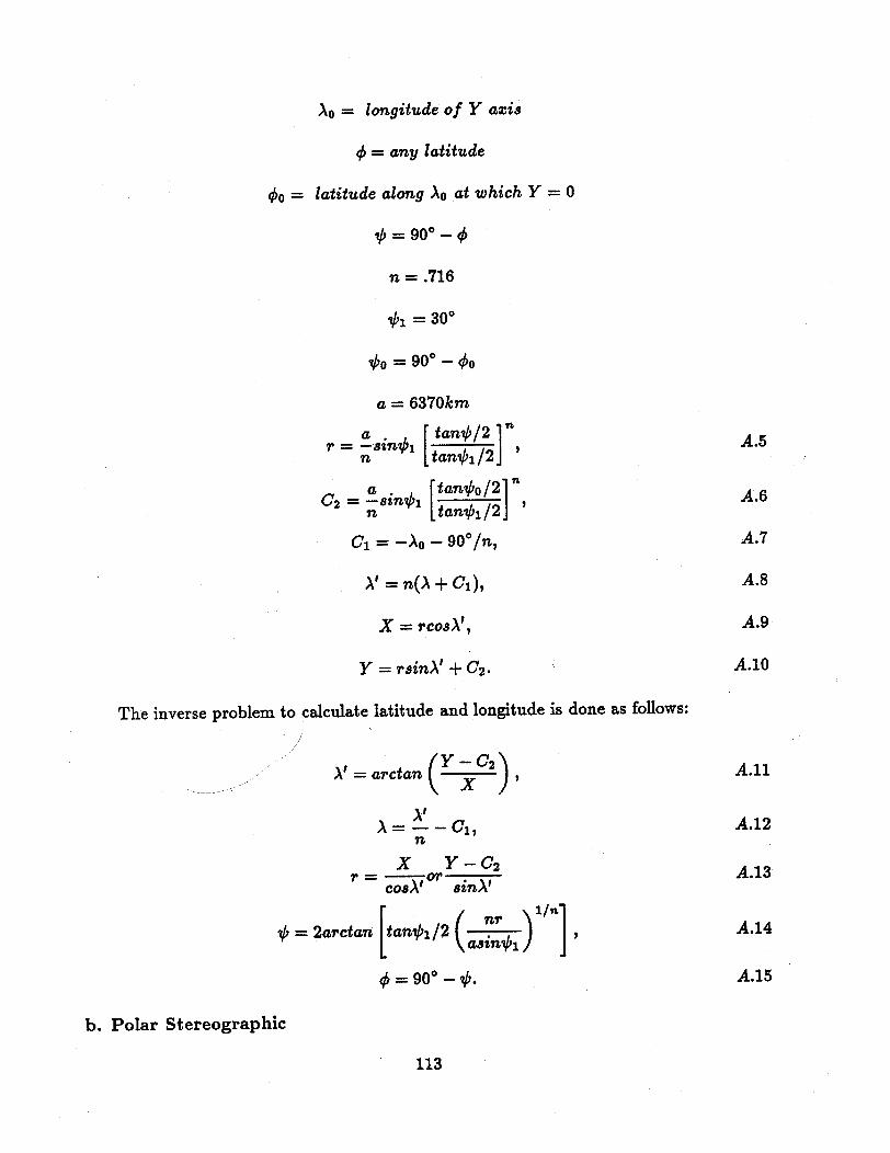
Ao = longitude of Y axis

b = any latitude

qo = latitude along oA at which Y = 0

- = 90-°

n .716

bl = 30°

bo = 900 - <0

a = 6370km

na n [tan71/2] ' A.5r ·- tni

=a = a[tant,,o/2 n A.6C2 - SMin01 ------ , A.6

n [tanji/2J

C1 = -A - 90/n, A.7

A' =n(A+Ci), A.8

X = rcosA', A.9

Y =rsin' + C2. A.10

The inverse problem to calculate latitude and longitude is done as follows:

A' = arctan (X2) , A.11

A= -C1, A.12n

X Y - C2.13-= orA.13cosA' sinA'

I = 2arctan tanbi/2 ( l ) , A.14

= 90 0 - . A.15

b. Polar Stereographic

113

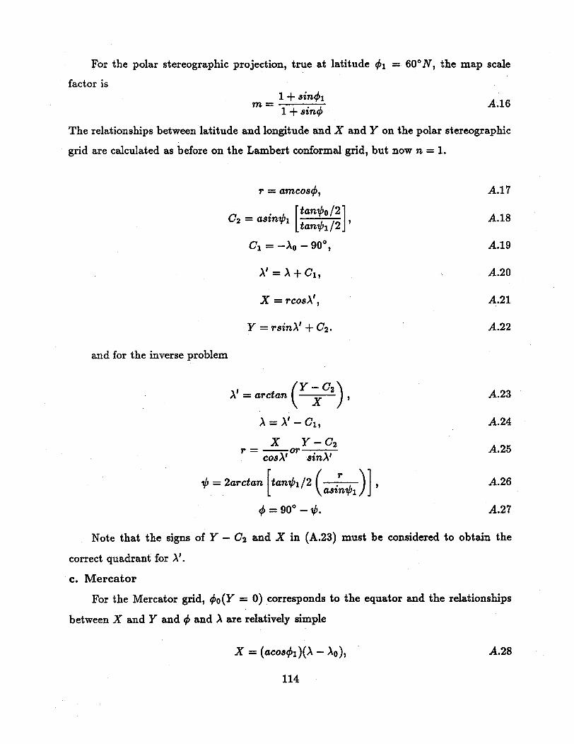
For the polar stereographic projection, true at latitude l1 = 60°N, the map scale

factor is1 + sinbl

m = . A.161 + sin"

The relationships between latitude and longitude and X and Y on the polar stereographic

grid are calculated as before on the Lambert conformal grid, but now n = 1.

r = amcosq, A.17

C 2 = asinb [tanbo /21 A.18

C1 = -oA -90°, A.19

Al = A + C1, -A.20

X =rcosA, A.21

Y = rsin + C2. A.22

and for the inverse problem

= arctan (Y C , A.23

A = Al C 1 , A.24

- Y - CA.25cosA' sinA

= 2arctan [tanbi /2 ( -- )], A.26asinol\

=900 - b. A.27

Note that the signs of Y - C 2 and X in (A.23) must be considered to obtain the

correct quadrant for A'.

c. Mercator

For the Mercator grid, qo(Y = 0) corresponds to the equator and the relationships

between X and Y and b and A are relatively simple

X = (acosi)(A - Ao), A.28

114

Y ( +l)lr [1 + sincos A.2a

y = (acosq)ln[tan(45° + 0/2)]. A.29b

Note that (A - Ao) in (A.28) must be expressed in radians. The latitude q1 at which the

Mercator projection is true is often taken to be 30°.

The reverse problem, to obtain X and Y from q and A, is also simple

XA-= AO +aos! A .30

acoso,

To solve for qb, use (A.29b)

=-90°+ r + 2ctan [e ( [ c-(7Y ) ] A.31' [ \~~~~acoso}\

115

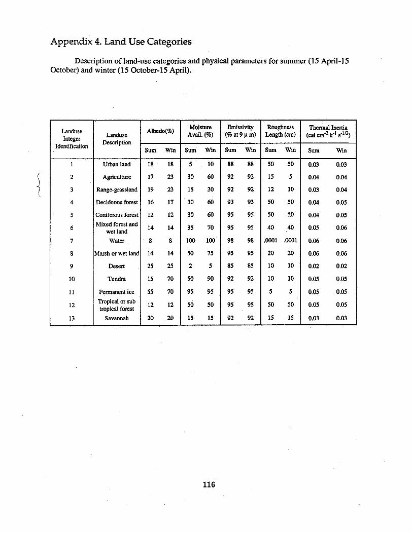
Appendix 4. Land Use Categories

Description of land-use categories and physical parameters for summer (15 April-15October) and winter (15 October-15 April).

116

C

kz

Moisture Emissivity Roughness Thermal InertiaLanduse Albedo(%)Landuse Landuse Ao) Avail. (%) (% at 9 A m) Length (cm) (cal cm-2 k-1 s- 2)

IntegerDescription :Identification

Sum Win Sum Win Sum Win Sum Win Sum Win

1 Urban land 18 18 5 10 88 88 50 50 0.03 0.03

2 Agriculture 17 23 30 60 92 92 15 5 0.04 0.04

3 Range-grassland 19 23 15 30 92 92 12 10 0.03 0.04

4 Deciduous forest 16 17 30 60 93 93 50 50 0.04 0.05

5 Coniferous forest 12 12 30 60 95 95 50 50 0.04 0.05Mixed forest and6 Mixed forest a 14 14 35 70 95 95 40 40 0.05 0.06wet land

7 Water 8 8 100 100 98 98 .0001 .0001 0.06 0.06

8 Marsh or wet land 14 14 50 75 95 95 20 20 0.06 0.06

9 Desert 25 25 2 5 85 85 10 10 0.02 0.02

10 Tundra 15 70 50 90 92 92 10 10 0.05 0.05

11 Permanent ice 55 70 95 95 95 95 5 5 0.05 0.05

Tropical or sub12 Tropical or sub 12 12 50 50 95 95 50 50 0.05 0.05tropical forest13 Savannah 20 20 15 15 92 92 15 15 0.03 0.03

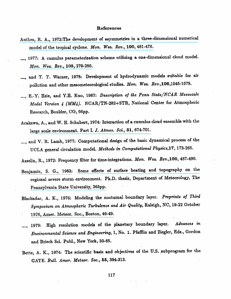
References

Anthes, R. A., 1972:The development of asymmetries in a three-dimensional numerical

model of the tropical cyclone. Mon. Wea. Rev., 100, 461-476.

_, 1977: A cumulus parameterization scheme utilizing a one-dimensional cloud model.

Mon. Wea. Rev., 105, 270-286.

_, and T. T. Warner, 1978: Development of hydrodynamic models suitable for air

pollution and other mesometeorological studies. Mon. Wea. Rev.,106,1045-1078.

_, E.-Y. Hsie, and Y.H. Kuo, 1987: Description of the Penn State/NCAR Mesoscale

Model Version 4 (MM4). NCAR/TN-282+STR, National Center for Atmospheric

Research, Boulder, CO, 66pp.

Arakawa, A., and W. H. Schubert, 1974: Interaction of a cumulus cloud ensemble with the

large scale environment. Part I. J. Atmos. Sci., 31, 674-701.

_, and V. R. Lamb, 1977: Computational design of the basic dynamical process of the

UCLA general circulation model. Methods in Computational Physics,17, 173-265.

Asselin, R., 1972: Frequency filter for time-integrations. Mon. Wea. Rev.,100, 487-490.

Benjamin, S. G., 1983: Some effects of surface heating and topography on the

regional severe storm environment. Ph.D. thesis, Department of Meteorology, The

Pennsylvania State University, 265pp.

Blackadar, A. K., 1976: Modeling the nocturnal boundary layer. Preprints of Third

Symposium on Atmospheric Turbulence and Air Quality, Raleigh, NC, 19-22 October

1976, Amer. Meteor. Soc., Boston, 46-49.

_, 1979: High resolution models of the planetary boundary layer. Advances in

Environmental Science and Engineering, 1, No. 1. Pfafflin and Ziegler, Eds., Gordon

and Briech Sci. Publ., New York, 50-85.

Betts, A. K., 1974: The scientific basis and objectives of the U.S. subprogram for the

GATE. Bull. Amer. Meteor. Soc., 55, 304-313.

117

Bleck, R., 1977: Numerical simulation of lee cyclogenesis in the Gulf of Genoa. Mon. Wea.

Rev., 105, 428-445.

Bougeault, P., 1983: A non-reflective upper boundary condition for limited-height

hydrostatic models. Mon. Wea. Rev., 111, 420-429.

Brown, J., and K. Campana, 1978: An economical time-differencing system for numerical

weather prediction. Mon. Wea. Rev., 106, 1125-1136.

Carlson, T. N., and F. E. Boland, 1978: Analysis of urban-rural canopy using a surface

heat flux/temperature model. J. Appl. Meteor., 17, 998-1013.

Davies, H. C., and R. E. Turner, 1977: Updating prediction models by dynamical

relaxation: An examination of the technique. Quart. J. Roy. Meteor. Soc., 103,225-

245.

Deardorff, J. W., 1972: Parameterization of the planetary boundary layer for use in general

circulation models. Mon. Wea. Rev., 100,93-106.

_, 1978: Efficient prediction of ground surface temperature and moisture, with inclusion

of a layer of vegetation. J. Geophys. Res.. 83, 1889-1903.

Delsol, F., K. Miyakoda, and R. H. Clarke, 1971: Parameterized processes in the surface

boundary layer of an atmospheric circulation model. Quart. J. Roy. Meteor. Soc.,

97, 181-208.

Dudhia, J., 1989: Numerical study of convection observed during the winter monsoon

experiment using a mesoscale two-dimensional model. J. Atmos. Sci., 46,3077-3107.

_, 1993: A nonhydrostatic version of the Penn State / NCAR mesoscale model: Validation

tests and simulation of an Atlantic cyclone and cold front. Mon. Wea. Rev., 121,

1493-1513.

Durran, D.R., and J.B. Klemp, 1982: On the effects of moisture on the Brunt-Vaisila

frequency. J. Atmos. Sci. 39, 2152-2158.

Fritsch, J. M., and C. F. Chappel, 1980: Numerical prediction of convectively driven

118

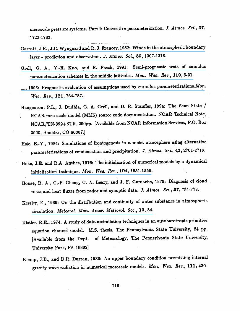
mesoscale pressure systems. Part I: Convective parameterization. J. Atmos. Sci., 37,

1722-1733.

Garratt, J.R., J.C. Wyngaard and R. J. Francey, 1982: Winds in the atmospheric boundary

layer - prediction and observation. J. Atmos. Sci., 39, 1307-1316.

Grell, G. A., Y.-H. Kuo, and R. Pasch, 1991: Semi-prognostic tests of cumulus

parameterization schemes in the middle latitudes. Mon. Wea. Rev., 119, 5-31.

_, 1993: Prognostic evaluation of assumptions used by cumulus parameterizations.Mon.

Wea. Rev., 121, 764-787.

Haagenson, P.L., J. Dudhia, G. A. Grell, and D. R. Stauffer, 1994: The Penn State /

NCAR mesoscale model (MM5) source code documentation. NCAR Technical Note,

NCAR/TN-392+STR, 200pp. [Available from NCAR Information Services, P.O. Box

3000, Boulder, CO 80307.]

Hsie, E.-Y., 1984: Simulations of frontogenesis in a moist atmosphere using alternative

parameterizations of condensation and precipitation. J. Atmos. Sci., 41, 2701-2716.

Hoke, J.E. and R.A. Anthes, 1976: The initialization of numerical models by a dynamical

initialization technique. Mon. Wea. Rev., 104, 1551-1556.

Houze, R. A., C.-P. Cheng, C. A. Leary, and J. F. Gamache, 1979: Diagnosis of cloud

mass and heat fluxes from radar and synoptic data. J. Atmos. Sci., 37, 754-773.

Kessler, E., 1969: On the distribution and continuity of water substance in atmospheric

circulation. Meteorol. Mon. Amer. Meteorol. Soc., 10, 84.

Kistler, R.E., 1974: A study of data assimilation techniques in an autobarotropic primitive

equation channel model. M.S. thesis, The Pennsylvania State University, 84 pp.

[Available from the Dept. of Meteorology, The Pennsylvania State University,

University Park, PA 16802]

Klemp, J.B., and D.R. Durran, 1983: An upper boundary condition permitting internal

gravity wave radiation in numerical mesoscale models. Mon. Wea. Rev., 111, 430-

119

444.

Klemp, J.B., and R.B.Wilhelmson, 1978: Simulations of three-dimensional convective

storm dynamics. J. Atmos. Sci., 35, 1070-1096.

Kuo, H. L., 1965: On formation and intensification of tropical cyclones through latent heat

release by cumulus convection. J. Atmos. Sci., 22, 40-63.

, 1974: Further studies of the parameterization of the effect of cumulus convection on

large scale flow. J. Atmos. Sci., 31, 1232-1240.

Lord, S., 1978: Development and observational verification of a cumulus cloud

parameterization. Ph. D. dissertation, University of California, Los Angeles, 359pp.

_1982: Interaction of a cumulus cloud ensemble with the large scale environment. Part

III: Semi-prognostic test of the Arakawa-Schubert parameterization. J. Atmos. Sci.,

39, 88-103.

Madala, R. V., 1981: Finite-Difference Techniques for Vectorized Fluid Dynamics

Calculations. Edited by D. L. Book, Springer Verlag, New York.

Marshall, J. S., and W. M. Palmer, 1948: The distribution of raindrops with size. J.

Meteor., 5, 154-166.

Montieth, J. L., 1961: An empirical method for estimating long wave radiation exchanges

in the British Isles. Quart. J. Roy. Meteor. Soc., 87, 171-179.

Perkey, D. J., and C. W. Kreitzberg, 1976: A time-dependent lateral boundary scheme for

limited area primitive equation models. Mon. Wea. Rev., 104, 744-755.

Richtmeyer, R. D., 1957: Difference methods for Initial- Value Problems. Interscience, New

York, 283pp.

Schubert, W. H., 1974: Cumulus parameterization theory in terms of feedback and control.

Atmos. Sci. Pap. No. 226, Colorado State University, 19 pp.

Sekhon, R.S., and R.C. Srivastava, 1970: Snow size spectra and reflectivity. J. Atmos.

Sci., 27, 299-307.

120

Shapiro, R., 1970: Smoothing, filtering and boundary effects. Rev. of Geophys. Space

Phy.,8,359-387.

Skamarock, W.C., and J.B. Klemp, 1992: The stability of time-split numerical methods

for the hydrostatic and nonhydrostatic elastic equations. Mon. Wea. Rev. 120,

2109-2127.

Smagorinsky, J., S. Manabe, and J. L. Holloway, Jr., 1965: Numerical results from a

nine-level general circulation model of the atmosphere, Mon. Wea. Rev., 93, 727-768.

Smolarkiewicz, P. K., and G. A. Grell, 1992: A class of monotone interpolation schemes.

J. Comp. Phys., 101, 431-440.

Stauffer, D.R. and N.L. Seaman, 1990: Use of four-dimensional data assimilation in a

limited-area mesoscale model. Part I: Experiments with synoptic-scale data. Mon.

Wea. Rev., 118, 1250-1277.

_, N.L. Seaman and F.S. Binkowski, 1991: Use of four- dimensional data assimilation

in a limited-area mesoscale model. Part II: Effects of data assimilation within the

planetary boundary layer. Mon. Wea. Rev., 119, 734-754.

_, and N.L. Seaman, 1993: On multi-scale four-dimensional data assimilation. J. Appl.

Meteor.,32, accepted for publication.

Zhang, D.-L., and R.A. Anthes, 1982: A high-resolution model of the planetary

boundary layer-sensitivity tests and comparisons with SESAME-79 data.J. Appl.

Meteor.,21,1594-1609.

_,H.-R. Chang, N. L. Seaman, T. T. Warner, and J. M. Fritsch, 1986: A two-way

interactive nesting procedure with variable terrain resolution. Mon. Wea. Rev.,

114, 1330-1339.

121