Hardware Software Synthesis of a H.264 / AVC Baseline ...

Rochester Institute of Technology Rochester Institute of Technology

RIT Scholar Works RIT Scholar Works

Theses

2005

Hardware Software Synthesis of a H.264 / AVC Baseline Profile Hardware Software Synthesis of a H.264 / AVC Baseline Profile

Decoder Decoder

Stephen P. Joralemon

Follow this and additional works at: https://scholarworks.rit.edu/theses

Recommended Citation Recommended Citation Joralemon, Stephen P., "Hardware Software Synthesis of a H.264 / AVC Baseline Profile Decoder" (2005). Thesis. Rochester Institute of Technology. Accessed from

This Thesis is brought to you for free and open access by RIT Scholar Works. It has been accepted for inclusion in Theses by an authorized administrator of RIT Scholar Works. For more information, please contact [email protected].

https://scholarworks.rit.edu/

https://scholarworks.rit.edu/theses

https://scholarworks.rit.edu/theses?utm_source=scholarworks.rit.edu%2Ftheses%2F7761&utm_medium=PDF&utm_campaign=PDFCoverPages

https://scholarworks.rit.edu/theses/7761?utm_source=scholarworks.rit.edu%2Ftheses%2F7761&utm_medium=PDF&utm_campaign=PDFCoverPages

mailto:[email protected]

Hardware Software Synthesis of a H.264 / Ave Baseline Profile Decoder

By

Stephen Paul Joralemon

A Thesis Submitted in Fulfillment of the Requirements for the Degree of Master of Science in Computer Engineering

Approved By:

Supervised by Visiting Assistant Professor Dr. Marcin Lukowiak

Department of Computer Engineering Kate Gleason College of Engineering

Rochester Institute of Technology Rochester, NY

Dr. Marcin Lukowiak, Visiting Professor Primary Advisor - R.l T Dept. of Computer Engineering

Dr. Roy Czemikowski, Professor Secondary Advisor - R.l T Dept. of Computer Engineering

Dr. Kenneth Hsu, Professor Secondary Advisor - R.l T Dept. of Computer Engineering

February 2005

Thesis/Dissertation Author Permission Statement

, H AR~wA,~ SO(-TwA2£ SytVntE£I$ C?,-=-'

J3:,A~g" II~e f~F"-.e.. Dl:!~C>;:'€../2

Name of author: STE~ t-\E.N >. J012,q4£JIIloAl

Degree: M ASTt..I'L d~ $c II;:: ,v kf: Program: CQI"'II~U7£Q ~ N(",N€'iFf2.IN("

College: \<. ArE C-, (...E:..4-.) <2ty C"kU; t;.. f "F

I understand that I must submit a print copy of my thesis or dissertation to the RIT Archives, per current RIT guidelines for the completion of my degree. I hereby grant to the Rochester Institute of Technology and its agents the non-exclusive license to archive and make accessible my thesis or dissertation in whole or in part in all forms of media in perpetuity. I retain all other ownership rights to the copyright of the thesis or dissertation. I also retain the right to use in future works (such as articles or books) all or part of this thesis or dissertation.

Print Reproduction Permission Granted:

I, S-q=:Pt!.E tv JaR ..At..-( naN , hereby grant permission to the Rochester Institute Technology to reproduce my print thesis or dissertation in whole or in part. Any reproduction will not be for commercial use or profit.

Signature of Author: ___________________ Date:

Print Reproduction Permission Denied:

I, , hereby deny permission to the RIT Library of the Rochester Institute of Technology to reproduce my print thesis or dissertation in whole or in part.

Signature of Author: ___________________ Date: _____ _

Inclusion in the RIT Digital Media Library Electronic Thesis & Dissertation (ETD) Archive

I, , additionally grant to the Rochester Institute of Technology Digital Media Library (RIT DML) the non-exclusive license to archive and provide electronic access to my thesis or dissertation in whole or in. part in all forms of media in perpetuity.

I understand that my work, in addition to its bibliographic record and abstract, will be available to the world-wide community of scholars and researchers through the RIT DML. I retain all other ownership rights to the copyright of the thesis or dissertation. I also retain the right to use in future works (such as articles or books) all or part of this thesis or dissertation. I am aware that the Rochester Institute of Technology does not require registration of copyright for ETDs.

I hereby certify that, if appropriate, I have obtained and attached written permission statements from the owners of each third party copyrighted matter to be included in my thesis or dissertation. I certify that the version I submitted is the same as that approved by my committee.

Signature of Author: ______________ Date: _____ _

Abstract

The latest video compression standard is a joint effort between ITU and MPEG known as

H.264/AVC. As with any video compression standard the H.264/AVC uses

computationally intensive algorithms to maximize performance. During decompression

these algorithms must be applied in real-time, processing 30 frames a second. This can

be done in software, specialized hardware, or a combination of the two. Software

solutions allow for maximum portability and ease of design, but General Purpose

Processors (GPP) can not take full advantage of the parallelizable algorithms that the

H.264 decoder is based upon. Specialized hardware solutions, on the other hand, allow

concurrent data and instruction paths, but do not offer a high level of abstraction for cross

platform development. Recent work by Xilinx has resulted in the advent of the

MicroBlaze soft-processor that is a stand alone microcontroller built from an FPGA. The

MicroBlaze provides a specialized hardware medium to run software on-chip with VHDL

entities.

The goal of this thesis was to model and simulate a software hardware hybrid

H.264/AVC Baseline Profile decoder using VHDL and a soft-processor. It was proposed

to divide all highly sequential calculations (run-length and CALVC decoding) and

control data flow into software and perform the remaining calculations (prediction,

inverse transform, inverse quantization, etc.) in hardware modules. The software runs on

Xilinx'

s MicroBlaze soft-processor and the hardware was designed using VHDL. A

major advantage of soft-processors over GPP's, is that it hardware instantiations reside

on-chip with the processor. The software and MicroBlaze soft-processor were simulated

in a test bench and the results proved that the MicroBlaze could not handle the encoded

bit-stream in real-time. For this reason the hardware interface and hardware decoder

were never fully implemented. The scope of the thesis covers the H.264 Baseline Profile

standard, MicroBlaze processor, the implemented software solution, and the proposed

hardware counterpart.

Table of ContentsOverview 1

1.1 H.264 Overview 1

1.2 Soft-Processor Overview 3

1.3 HW/SW Hybrid H.264 Decoder Design 5

Background Theory 7

2.1 Video Compression 7

2.1.1 Frames and Fields 8

2.1.2 Color 8

2.1.3 Format 9

2.2 H.264/AVC Standard 11

2.2.1 Network Abstraction Layer (NAL) and Video Coding Layer (VCL) 12

2.2.2 Macroblocks and Slices 13

2.2.3 Intra Prediction 14

2.2.4 Inter Prediction 17

2.2.5 Transform and Quantization 20

2.2.6 Entropy Coding 24

2.2.7 Deblocking Filter 26

2.3 MicroBlaze Soft-Processor 27

2.3.1 Processor Architecture 27

2.3.2 Processor Busses 29

2.3.3 Interrupts, Breaks, and Exceptions 32

2.3.4 Kernel and Drivers 32

HW/SW Hybrid H.264 Decoder Design 34

3.1 Hardware Architecture 35

3.1.1 AVC File Interface Module (External) 36

3.1.2 OPB RelayModule 37

3.1.3 AVC Decoder Core 39

3.2 Software Architecture 42

3.2.1 Software Design Process 42

3.2.2 Top Level Functionality 43

3.2.3 Reading the Bit-Stream 44

3.2.4 AVC Decoder Core Interface 45

Test Bench and Results 46

4.1 Encoded Bit-Stream 46

4.2 Feeding the Decoder 46

4.3 Results 48

Conclusion 51

5.1 Future Work 51

5.1.1 CAVLCCore 52

5.1.2 Buffer Core 54

in

List of Figures

Figure 1: H.264 Baseline Profile Decoder[1] 2

Figure 2: MicroBlaze Core Block Diagram 4

Figure 3: YC,Cb SamplingFormats[,] 10

Figure 4: H.264 StandardProfiles111 11

Figure 5: NAL Format 12

Figure 6: Subdivision of a Frame into Slices and SliceGroups[8] 14

Figure 7: 4x4 Intra Prediction Patterns (sub-block) 15

Figure 8: 16x16 Intra PredictionPatterns131 16

Figure 9: Tree Structured Macroblock Partitions 17

Figure 10: Optimal Block Partitioning for IntraPrediction1'1 18

Figure 11: Sub-pixel Mappings for InterPrediction1 1]

19

Figure 12: 16x16 Macroblock BlockOrdering151

24

Figure 13: Raster Scan Orders for Decoding 24

Figure 14: IPIC Bus Read and Write Sequence 32

Figure 15: HW/SW Hybrid H.264 Decoder 35

Figure 16: XPS HW/SW Hybrid Decoder Layout 36

Figure 17: H.264 Decoder HW/SWDivision

39

Figure 18: HW/SW Hybrid H.264 Decoder Test Bench 47

Figure 19: Proposed Hardware Design 52

Figure 20: CAVLC Core 53

Figure 21: Buffer Core 55

IV

List of Tables

Table 1: Video Formats 10

Table 2: PF Look-up Table 22

Table 3: Qstep Look-up Table 22

Table 4: Exp-Golomb Entropy Code Number Ranges 25

Table 5: coeff_token Table Look-up Table 26

Table 6: MicroBlaze Register Bank 28

Table 7: SystemMemory Map 36

Table 8: OPB Relay Signals 38

Table 9: Hardware Address Table for the H.264 Decoder Core 41

Table 10: Function Calling Tree 49

Table 11: Software Timing Statistics (lis) 49

Glossary

ASIC - Application Specific Integrated Circuit - A specialized hardware designed aimed

at a specific application. Pg. 3.

AVC - Advanced Video Code - The latest video compression standard and topic of this

paper, Pg. 1, 11, Section 2.2

BRAM - Block Random Access Memory -

Memory located on-chip with the FPGA and

available to theMicroBlaze soft-processor, Pg. 5.

CABAC - Context-Adaptive Binary Coding An efficient coding algorithm geared

towards streams with a fixed table of transmitted data, Pg. 10, 24.

CAVLC - Context-Adaptive Variable Length Code - An encoding scheme used by AVC

to encode data at the bit-level, Pg. 25, Section 2.2.6.2

CODEC - Video enCODer DECoder pair. Pg.7, 21.

DCT - Discrete Cosine Transform - A matrix transform common in image and video

compression standard that converts data from the spatial domain into a frequencydomain. Pg 1, 21.

DMA - Direct Memory Transfer- The transfer of data directly between two modules on

a bus without going through the main processor. Pg. 5, 30.

DSP - Digital Signal Processor - Processor with an architecture specifically designed for

digital signal computations. Typically DSP's provide parallel data paths with an

ISA that offers vector instructions. Pg. 2-3.

EDK - Embedded Development Kit - Xilinx software kit that provides for the design and

integration of combined software and hardware solutions, Pg. 5.

FPGA - Field Programmable Gate Array - A programmable logic chip with a high

density of gate arrays. Pg.2.

FSL - Fast Simplex Link - A simplified bus that connects directly to the registers in a

MicroBlaze soft-processor core, Pg. 29, Section 2.3.2.1.

GPP - General Purpose Processor - Typical microprocessor available commercially

without any specialized hardware for targeted applications. Pg. 2.

H.264 -see AVC.

HVS - Human Visual System - A term that encapsulates the manner which humans

sample and process visual stimuli, Pg. 9.

IP - Intellectual Property- Within the scope of this paper IP refers to modules design by

Xilinx that attach to a soft-processor bus. Pg. 26.

IPIC - Intellectual Property Inter-Connect- A hardware template designed by Xilinx to

connect hardware to a soft-processor bus, Pg. 5, 31.

IPIF - Intellectual Property Interface - The actual hardware interface that connects the

OPB to the IPIC, Pg. 5, 31.

ISA - Instruction Set Architecture - Set of program instructions that are available for a

given processor. Pg. 3, 21.

ITU - International Telecommunications Union - An organization that shares the goal in

standardizing video media, Pg. 1.

LMB - Local Memory Bus - MicroBlaze's memory bus that is used to connect to

BRAM, Pg. 5, 29, 31, Section 2.3.2.2..

MPEG - Motion Picture Experts Group - An organization that shares the goal in

standardizing video media, Pg. 1.

VI

NAL - Network Abstraction Layer - A layer in the AVC encoding protocol that includes

and identifies the contents of an AVC packet of data, Pg. 11, Section 2.2.1.

OPB -

On-chip Peripheral Bus - MicroBlaze's bus used to connect to peripherals

including memory. Pg. 4, 30, Section 2.3.2.3.

PLB - Processor Local Bus A synchronous bus that connects the processor to high

speed and high-performance I/O. Pg. 4, 30, Section 2.3.2.4.

QP - Quantization Parameter -

Scaling factor used by the decoder during inverse

quantization. Pg. 21.

RGB - Red, Green, Blue - A Common color space used for capturing and displaying

visual multi-media. Pg 7, Section 2.1.2.1.

SAE - Sum of Absolute Errors - Method of calculation to measure the error of a given

prediction. Pg. 15.

VCL - Video Code Layer - A layer in the AVC encoding protocol that includes actual

video data, Pg. 11, Section 2.2.1.

VHDL - VHSIC (Very High Speed Integrated Circuit) Hardware Description Language

- Language used to model and design hardware from the gate level to algorithm

level. Pg 2.

XPS - Xilinx Platform Studio - Development software that allows a user to design both

hardware and software separately, then combine and test, Pg .35.

YCrCb - A three component color-space that is used by AVC, Pg. 9, Section 2.1.2.2.

VII

1 Overview

1.1 H.264 Overview

As digital video entered the air waves, cable, and optical storage devices in a massive

scale two major standardization groups took on the field of video compression, the

International Telecommunications Union (ITU) and Motion Picture Experts Group

(MPEG). The ITU is recently known for its H.261 and H.263 publications while the

MPEG's claim to fame has been the MPEG-1 and MPEG-2 video standards. Beginning

in 1997 the two groups combined efforts to put together the next generation video

compression standard. In 2003 the H.264, a.k.a. MPEG-4 Part 10, a.k.a. Advanced Video

Code (AVC), standard was finalized. The new standard offers several improvements to

its predecessors (H.261, H.262/MPEG-2, and H.263) such as:[8]

? Variable block-sizes ranging from 16x16 to 4x4

? Va pixel resolution for motion prediction

? Multiple reference frames for temporal residual calculation

? Introduction of an integer form of the Discrete Cosine Transform

The new features target a 2x improvement in bit compression while yielding consistent

quality'91. Note that with improvements in compression come an increase in algorithm

complexity and thus computation load. The scope of this document concentrates on the

decompression side of an H.264 bit-stream.

It is the responsibility of the decoder to reconstruct the compressed data into a

representation of the original video signal. A block diagram of an H.264 decoder may be

found in Figure 1. Upon reception of the bit-stream, it is sent through an entropy decoder

to extract the video header information and the actual video data. Next, the run-length

decoder adds any data redundancies that were removed for compression. The data is then

scaled, reordered, and sent through the inverse integer Discrete Cosine Transform (DCT).

The resulting bits represent the spatial (intra) and temporal (inter) predications of the

encoder and the corresponding difference or residual from the actual values. A history of

reconstructed images must be kept for inter prediction; this buffer mimics one that is kept

within the encoder. The difference is combined with the prediction to generate the actual

pixel values. Finally a deblocking filter is passed over the data to smooth the image. The

H.264 standard defines three profiles of operation, Baseline, Main, and Extended, each

profile adds a level of flexibility to the standard. The Baseline Profile is the only profile

covered in the thesis. However, the hardware and software is modularized in a way to

facilitate the addition of the other two profiles.

F'n-1(reference)

Inter

Prediction

Encoded

Bit Stream

SEntropyDecoder

Intra

Prediction

(reconstructed)Filter

uF',

CAVLC

Inverse

Quantizer

Inverse

Transform

Figure 1: H.264 Baseline Profile Decoderm

Decompressing a video sequence entirely on a GPP requires a large commitment which

draws computational resources from other applications running on the same processor.

As an alternative, specialized hardware such as an FPGA or DSP may be used to

decompress the video. An FPGA can process the bit-stream in fewer clock cycles than a

single CPU that is inherently sequential. Following this ideology, recent work has been

done to model a H.264 decoder in VHDL[7]. However, hardware design is a time

consuming process that does not offer the portability and flexibility of software. A

design is often tightly coupled to specific hardware peripherals and very little

functionality is abstracted. Consequently hardware designs are ported with greater

difficulty when compared to software solutions. A DSP Instruction Set Architecture

(ISA) offers the advantages of specialized instructions to handle signal processing

applications. Several H.264 decoders running on DSP's began to hit themarket towards

the end of 2004[IOH12]. Note that almost all the software solutions decode a max

resolution of 352x288 (CIF).

An alternative H.264 decoder design would be a combined software hardware solution.

A new breed of processing has become commercially available allowing a user to turn an

FPGA into a microcontroller. This computational unit has been dubbed a soft-processor.

Hardware modules, or VHDL entities, can be accessed by the soft-processor providing

the benefits of a pipelined processor on-chip with parallelizable hardware instantiations.

The main advantage of a soft-processor over a DSP is that hardware instantiations may be

developed on-chip with the processing unit aimed at performing specialized operations.

The soft-processor also provides a unique opportunity for design migration. That is, a

complete software application may be developed in an expedited manner. Bottlenecks

within the software can be identified and moved to hardware. Thus as a design

progresses the FPGA may be reconfigured for better performance without affecting

external hardware. Note that a natural high-level division for the H.264 standard exists

after run-length decoding and before inverse quantization. Everything prior is naturally

sequential and everything after parallelizable to some extent. For the decoder design the

run-length and entropy decoder will run on the MicroBlaze CPU and the remaining

calculations performed in a VHDL entity.

1.2 Soft-Processor Overview

Xilinx in fact offers three soft-processors. They are, listed in increasing complexity,

PicoBlaze, MicroBlaze, and a PowerPC based microcontroller. The PicoBlaze is limited

to small applications that do not require a lot of processing. Although diverse, the

PowerPC is a bit large for this particular application and would lengthen the development

time. Note that Xilinx also offers boards with PowerPC controllers on them; this is not

the same as a soft-processor. For these reasons the MicroBlaze processor was chosen to

control the I/O and execute the software side of the design. MicroBlaze is able to address

enough RAM to execute the code required and uses fewer gates than the PowerPC. The

following is a summary of the MicroBlaze soft-processor based on documentation

provided by Xilinx. For a complete description of the MicroBlaze architecture, kernel,

and programming interface please refer to references [14]"[17].

MicroBlaze is a 32-bit load/store RISC processor (Figure 2) with 32 32-bit general

purpose registers to handle addressing, interrupts, and the instruction set. The soft-

processor architecture includes a 3-stage pipeline consisting of a fetch, decode, and

execute stage. The arithmetic logic unit provides a limited set of operations excluding

floating point arithmetic. Memory can be accessed by byte (8-bit), half-word (16-bit),

and word (32-bit). All data and addresses are in big endian form.

MDM

t

Debug Logic

FSL

Local Link l/F

Address

Side

LMB

l-LMB

Instruction

Cache

l-OPB

Program

Counter

I

Control Unit

Instruction

Buffer

Register

Bank

32x32-bit

Machine Status

Register

Logical /

Shift

Barrel

Shifter

Divider

ALU

Multiply J"

Data

Side

LMB

D-LMB

Data

Cache

D-OPB

PERIPHERALS

Interrupt Controller UART

OPB CoreConnect

Off-Chip

Memory 0-4GBWatchdogTimer

General

Purpose I/O

OPB CoreConnect

Timer /

Counter

Off-Chip

Memory 0-4GB

Xilinx

Figure 2: MicroBlaze Core Block Diagram

There are three processor busses available and compatible to the MicroBlaze soft-

processor, all ofwhich are based on the IBMCore-Connect

bus standards. Two of these

busses provide access to external peripherals and VHDL modules, the On-chip Peripheral

Bus (OPB) and Processor Local Bus (PLB). The PLB is a synchronous bus that connects

the processor to high-speed and high-performance I/O. It has separate lines for address,

data read, and data write signals. This permits the PLB to provide simultaneous read and

write operations to expedite I/O. The OPB is a general purpose bus with a simplified

interface. The data read and data write signals share a common data path; therefore, the

OPB does not permit concurrent read and write operations. All of the peripherals

connected to the OPB are memory mapped and accessible by writing or reading to the

specified address. Both the OPB and PLB support DMA to relieve the processor work

load while transferring data. The final bus is theMicroBlaze'

s Local Memory Bus

(LMB). The LMB connects the processor to internal on-chip Block RAM (BRAM).

BRAM can be used for instruction memory, data memory, or both.

Xilinx'

s Embedded Development Kit (EDK), the MicroBlaze development suite,

provides several templates to connect user defined logic modules onto the IBM Core-

Connect bus'151. The templates are known as Intellectual Property Inter-Connects (IPIC)

that provide a range of address, data, and status signals to control and communicate with

any given VHDL module. The IPIC used is based on the functionality of the device and

whether it needs to be a master bus device or can function as a slave. The IPIC is further

wrapped inside an IP Interface (IPIF) module that is the actual connection to the bus and

accesses the processor through a module known as an OPB Arbiter (the Arbiter acts as

the actual bus controller). The IPIF layer is transparent to the user; only the IPIC needs

to be directly interfaced with. This gives a programmer quick access to the bus without

an in-depth knowledge of the bus protocol. Putting the decoder into the IPIC module

provides platform independence within the EDK suite of processors. The IPIC is a

generic interface that will interface with all of the IPIF units and OPB that exist. Any

future changes that Xilinx makes to the bus will be incorporated into the IPIF interface.

Portability for future work is one of the major design goals of the thesis.

1.3 HW/SW Hybrid H.264 Decoder Design

The hardware/software hybrid decoder was developed using the Xilinx EDK suite. EDK

provides utilities for generating hardware (VHDL) modules, compiling and linking code

(gcc), porting designs to ModelSim for simulation, and porting designs to Project

Navigator for mapping onto a specified FPGA. The overall hardware design connects a

MicroBlaze soft-processor to local BRAM for instruction and data memory. A relay

hardware module was designed to connect both a partial hardware AVC Decoder Core

and AVC File Core interface to the MicroBlaze. The AVC Decoder Core takes a frame

of 4x4 coefficient matrices and control data as input and outputs pixels of the decoded

frame.

It is the responsibility of the software to read the bit-stream from the AVC File Core,

decode the data, and send the resulting coefficients to the AVC Decoder Core. The AVC

File Core was designed using VHDL to read an H.264 ASCII file and also provides a

very primitive write interface. Once the AVC Decoder Core has decoded a full frame the

software reads in the frame from the AVC Decoder Core and writes it out to file using the

AVC File Core. The resulting file contains pixel representations of the decoded video

stream.

2 Background Theory

2.1 Video Compression

The aim of video compression is to minimize the amount of data required to represent a

given sequence of images and in turn reduce transmission payloads and storage

requirements. There are two categories of compression, whether in data, image, or video

processing, known as lossless and lossy. The former technique constitutes that an exact

replica of the original image can be generated from the encoded data, no information is

lost. This technique is useful when the data has a high priority such as medical images.

Lossless algorithms involve decreasing data entropy without loss of information. The

second category, lossy, constitutes that some information is lost and comprises much of

the transmitted data applications today. The goal of lossy algorithms is to remove low

priority or irrelevant data without jeopardizing the integrity of the video sequence. The

main design tradeoff is compression rate verse the quality of the decompressed video.

The more aggressive the encoder is the greater the reduction of quality in the decoded

video. The H.264 Standard uses both lossy and lossless techniques. For example,run-

length encoding (a lossless technique) is used to encode binary level information while

rounding and quantization (a lossy technique) is used to encode residual coefficients.

Video compression encapsulates the encoding, transmission or storage, and decoding of

data. Transmission and storage will not be discussed in detail in this paper; however, it is

worth noting since compression has a direct effect on bandwidth and capacity

requirements. An encoder decoder pair (CODEC) must agree on the compressed data

format in order to sustain compatibility. Video compression standards in fact only define

the compressed data format. In doing so, encoder implementation and algorithm design

is open for interpretation. Two encoders may be entirely different, but the bit-stream that

they produce must adhere to the standard. This method of standardization provides that

the decoder may translate data produced from any encoder.

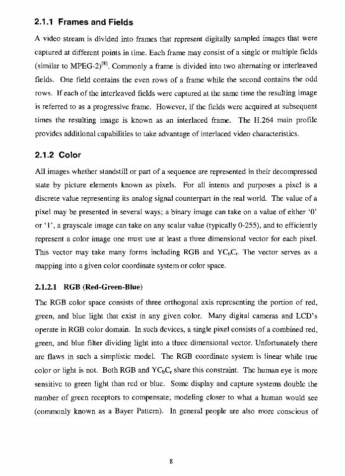
2.1.1 Frames and Fields

A video stream is divided into frames that represent digitally sampled images that were

captured at different points in time. Each frame may consist of a single or multiple fields

(similar to MPEG-2)[8]. Commonly a frame is divided into two alternating or interleaved

fields. One field contains the even rows of a frame while the second contains the odd

rows. If each of the interleaved fields were captured at the same time the resulting image

is referred to as a progressive frame. However, if the fields were acquired at subsequent

times the resulting image is known as an interlaced frame. The H.264 main profile

provides additional capabilities to take advantage of interlaced video characteristics.

2.1.2 Color

All images whether standstill or part of a sequence are represented in their decompressed

state by picture elements known as pixels. For all intents and purposes a pixel is a

discrete value representing its analog signal counterpart in the real world. The value of a

pixel may be presented in several ways; a binary image can take on a value of either'0'

or '1', a grayscale image can take on any scalar value (typically 0-255), and to efficiently

represent a color image one must use at least a three dimensional vector for each pixel.

This vector may take many forms including RGB and YCbCr. The vector serves as a

mapping into a given color coordinate system or color space.

2.1.2.1 RGB (Red-Green-Blue)

The RGB color space consists of three orthogonal axis representing the portion of red,

green, and blue light that exist in any given color. Many digital cameras and LCD's

operate in RGB color domain. In such devices, a single pixel consists of a combined red,

green, and blue filter dividing light into a three dimensional vector. Unfortunately there

are flaws in such a simplistic model. The RGB coordinate system is linear while true

color or light is not. Both RGB and YCDCr share this constraint. The human eye is more

sensitive to green light than red or blue. Some display and capture systems double the

number of green receptors to compensate; modeling closer to what a human would see

(commonly known as a Bayer Pattern). In general people are also more conscious of

changes in luminance rather then color or hue. It is desirable to directly represent the

intensity at each pixel to map to the Human Visual System (HVS).

2.1.2.2 YCbCr

YCbCr was derived to increase the resolution of luminance (Y) within the color space.

RGB maps three basis colors equally even though the human eye is more sensitive to

luminance rather then color. The magnitude of the RGB vector is more important than

the composition. The YCt>Cr space dedicates an axis (Y) to luminance to maximize the

resolution and in turn adapt to the HVS.

The Luma component (Y) is a weighted average of the red, green, and blue components

(Equation 1) where kr, kg, and fa, are some weighting factors. The chrominance

components, Cr and Cb, are derived from the Luma. There is also an unspoken Cg

component that can be calculated either from the green component in RGB and Y

component in YCbCr or directly from the Cb and Cr components. The H.264 standard

operates in the YCbCr color space.

Y = krR + kgG + kB Eq.l

C=B-Y

Ch=R-Y Eq.2

Cg=G-Y

2.1.3 Format

There are several ways to spatially sample an analog image or video. The straight

forward approach would be a consistent rate across all components of a color space, a

grid of color components. However, to tailor to the HVS it is best to sample at higher

rates where the human eye is most sensitive. As far as the human eye is concerned,

intensity has the highest priority. Therefore, intensity should have the highest resolution.

Figure 3 demonstrates three different sampling configurations in the YCbCr space. The

first, 4:4:4, samples at the same resolution across all components. 4:2:2 implies that there

are twice as many Luma components as Chroma. To achieve this, the chrominance

components are sampled every other column. The 4:2:0 format is counter intuitive in its

naming. 4:2:0 sampling produces a single Cb and Cr for every four Y samples. The

chroma samples are located every other column between every two Luma rows.

Typically each color component, whether a luma or chroma, ranges from 0 to 255

requiring 24-bits to represent a complete pixel in 4:4:4. 4:2:0 on average uses 12-bits to

represent a single pixel and is used in the H.264 standard.

% \_) V J

^HP % %

% vJ O %

((gk(pij) \_) %

% o % o

0 % o

%> o % o

h o (0 o

4:4:4

o o o o\t"":':'J \ )

o o o o

o o o o

(^ )o o o o

4:2:2

(_) Intensity Components

CrCb Components

4:2:0 0 lain E. G. Richardson

Figure 3: YCrCb SamplingFormats"1

Several video formats exist that span multiple sampling rates, image sizes, and frame

rates. Table 1 highlights a few that may be found in Appendix A in [1].

Format LumaWidth Luma Height MBs Total Luma Samples

SQCIF 128 96 48 12288

QCIF 176 144 99 25344

QVGA 320 240 300 76800

CIF 352 288 396 101376

VGA 640 480 1200 307200

4CIF 704 576 1584 405504

SVGA 800 600 1900 486400

4VGA 1280 960 4800 1228800

SXGA 1280 1024 5120 1310720

16CIF 1408 1152 6336 1622016

4SVGA 1600 1200 7500 1920000

16VGA 2560 1920 19200 4915200

Table 1: Video Formats

10

2.2 H.264/AVC Standard

The fundamentals of the H.264 standard are based on the accomplishments of its

predecessors H.261 and H.263. The actual compression is achieved by removing spatial

redundancy within a frame, temporal redundancy within a frame sequence, and data

redundancy within the bit-stream. Often the spatial domain is not the most efficient

space to work in. Many standards define a transform to convert data into the frequency

domain such as the Fourier or Discrete Cosine Transform. The idea is that high

frequencies in an image may be removed without risking the integrity of the data. It is

quite difficult to separate high frequency data in the spatial domain, while in the

frequency domain it is a simple threshold. The H.264 standard uses an integer version of

the Discrete Cosine Transform (see Section 2.2.5).

Extended profile

Main profile

j) lain E. G. Richardson

Figure 4: H.264 StandardProfiles"1

The H.264 defines three profiles within the overall standard; Baseline, Main, and

Extended (Figure 4). Each profile adds a level of flexibility and complexity to the bit-

stream. The Baseline Profile includes all of the basic definitions in order to decode the

most basic compressed stream. The Main Profile defines functionality for interlaced

video and Context-Adaptive Binary Coding (CABAC). CABAC is an efficient coding

algorithm geared towards streams with a fixed table of transmitted data. The Extended

11

Profile defines additional slices (section 2.2.2) and data partitioning. Data partitioning

provides a prioritization scheme within the encoded video. Only the Baseline Profile was

implemented in this thesis; however, the hardware and software designs are modularized

such that the additional profiles may be added in the future.

2.2.1 Network Abstraction Layer (NAL) and Video Coding Layer (VCL)

The H.264 bit-stream is divided and processed in two layers; the NAL and VCL. The

former is directed toward making the bit-stream transmission compliant and the latter

defines the actual format that encoded video data must adhere to. It is the responsibility

of the NAL to encapsulate the data produced by the VCL.

Start Code Prefix Header Byte Payload

Figure 5: NAL Format

The H.264 NAL defines NAL units that packet the coded video and non-video data

(Figure 5). A NAL unit consists of a start jprefix, a single header byte, and the

corresponding payload. The first bit of the header is always zero (forbidden_zero_bii),

bits 1-2 represent the NAL reference ID (naljrefjdc), and bits 3-7 identify what type of

data (naljunitjype) is contained within the appended payload. The beginning of a NAL

unit is marked with a byte aligned NAL delimiter or start jprefix (0x00000001).

Within the NAL unit emulation_prevention_bytes (0x03) are used to prevent a start code

prefix from occurring in the data. NAL unit payloads are categorized into VCL and non-

VCL units. The payload of a VCL unit contains actual encoded video data that translates

12

into frames. The payload of a Non-VCL unit contains information that describes the

format of the video and bit-stream. This information serves as headers for the video data

known as parameter sets. A parameter set can apply to the entire video sequence

(sequence parameter set) or to a set of pictures (picture parameter set) within the video

sequence. The NAL reference ID (nal_ref_idc) within a VCL NAL unit defines to which

picture parameter set the enclosed frame belongs. In turn, the picture parameter set has a

NAL reference ID to identify which sequence parameter set it belongs to.

As stated earlier the VCL contains the actual encoded video frames. The H.264 is a

block-based hybrid decoding standard[8]. That is, the image is broken down into

rectangular blocks and both temporal and spatial predictions are performed. The residual

of the predictions and the predictions themselves are encoded into the payload within a

VCL NAL unit.

2.2.2 Macroblocks and Slices

It is common for video compression standards to subdivide a frame into rectangular

blocks for processing known as macroblocks. All of ITU's recommendations starting

with the H.261 use this blocking method. The H.264 defines a macroblock as a 16x16

luminance region and its corresponding 8x8 chrominance values (refer to Figure 3). Note

that one of the major advances that the H.264 offers is the ability to encode sub-

macroblocks down to 4x4 lumina pixel and 2x2 chroma pixel blocks for motion

prediction (see Section 2.2.4). A series of macroblocks are grouped together into a slice.

An image may be composed of a single or several slices. Furthermore, slices that share

properties can be combined into slice groups. Slice groups have no geometric constraints

and can take on many patterns such as a checker-board, alternating lines, and object

based (Figure 6). Macroblocks within a slice are processed in a raster scan order. The

slices are decoded in the order that they are read or received. A group ofNAL units that

result in a decoded picture are known as an access unit. Access units are optionally

marked with access unit delimiters.

13

i i i : :

i i Slice #0 |i i i i i

j..j

i ! Slice #1

! ! ! !

ill:

: : Slice #2 I

: i i i i

Frame subdivided into Slices Frame subdivided into Slice Groups

isn pe Grot

r

I 1

p#2

Slic i G rou| )#0

^ :

Slic s G rou| i#1

_PL_ll_JH_pi_

Ii

Frame subdivided into Slice Groups Frame subdivided into Slice Groups

W. Wiegand, G. J. Sullivan, G. Bjontegaard, A. Luthra

Figure 6: Subdivision of a Frame into Slices and SliceGroups'81

The H.264 standard defines 5 different types of slices I, P, SI, SP, and B. A Baseline

Profile bit-stream may only include I and P slices. For a description of the other 3 slices

refer to [1]. An I slice contains macroblocks that are encoded using intra prediction.P-

slices contain macroblocks that are encoded using both inter and intra prediction. It is the

responsibility of the encoder to determine which method yields the highest compression

rate and group them into slices accordingly. Intra prediction algorithms remove spatial

redundancy and uses adjacent previously encoded unfiltered macroblocks. Inter

prediction algorithms remove temporal redundancy and use macroblocks from previously

encoded frames that have been filtered.

2.2.3 Intra Prediction

In intra prediction (I or P-slices) a block prediction is found using previously encoded

macroblocks that neighbor the current macroblock. Intra prediction may occur at both

the luma macroblock (16x16) and sub-block (4x4) levels. There are 9 possible prediction

modes for a sub-block and 4 possible prediction modes for macroblocks (Figure 7 and

Figure 8 respectively). An 8x8 chroma region has four intra prediction modes that mimic

the luma 16x16 modes. However, the ordering is different; DC (mode-0), horizontal

14

(mode-1), vertical (mode-2), and plane (mode-3)[3]. If the corresponding luma pixels are

encoded using intra prediction the chroma pixels must follow suit. In order to calculate

the predicted values for the current block pixels A-D and I-L must be processed (Figure

7). IfE-H have not been encoded then the value ofD is copied into their place. It is the

responsibility of the encoder to find the optimal intra prediction mode. One measurement

of quality is to correlate the Sum of Absolute Errors (SAE), the smaller the SAE the

greater the compression rate[3]. When encoding, once a prediction mode has been chosen

the residuals between the actual and predicted values are sent to the integer transform and

quantizer blocks Figure 1).

0 - Vertical1 - Horizontal

M A B Ci E F G H

1-

J-

K-

....,

'

Mean(-A-Jr-

3 -D agonal Down-Lefl

M A B C E F G H

I /V'/J /^i;k V

4 - Dl gon al Down-Righ

M A B C D E F G H

I \J

\L \

Right

6 - Horizontal Down

M, A B. c D E F G H

1^

^'v^

J^*V %

-

M

1

A

- Ve

B

rtica Lett

PE F G H

1.v '/ /J / /K

J /I / /

- Horizontal Up

M A B C 0 E F G H

1.

J,

K^

L.

) lain E. G. Richardson

Figure 7: 4x4 Intra Prediction Patterns (sub-block)

15

0 - Vertical

1 1 1 1 1 1 1 1 1 1 1 1 1 II

vV;.,^;^;,-,'^...,,

1 - Horizontal

J. I I I M I I I I

-

I.. >

"'

of* '':%'"'

a '''

&ff$4'

0/f: %

;;::'p'i

; ?

2 - Mean

i i i i i i i i i | ii i i r

Mean(H + y)-

3 - Plane

lain E. G. Richardson

Figure 8: 16x16 Intra Prediction Patterns[3]

The intra prediction mode for each block must be sent to the decoder adding additional

information and bits to the decoded stream. To limit the overhead required for intra

prediction further redundancy is removed. Neighboring blocks often share characteristics

including their prediction modes. To take advantage of this commonality, both the

encoder and decoder calculate the mostjprobablejnode of prediction for the current

block. If the macroblock above and the macroblock to the left are within the same slice

and coded in 4x4 Intra mode then the mostjprobablejnode is the minimum mode of the

two. Note that the mode values are included in Figure 7 and Figure 8 next to the

corresponding prediction type text. If the macroblock above and the macroblock to the

left are not of the same slice or encoded by other means then the mostjprobablejnode is

set to 2, DC. The encoder sends a flag for each 4x4 luma block telling the decoder

whether the mostjprobablejnode is used or not. If another mode of prediction is applied

then a 3-bit remainingjnode_selector is sent to identify which prediction method to

implement. If the new prediction mode is less than the mostjprobablejnode then the

remainingjnodejselector is set equal to the mode. If the new prediction mode is greater

than the mostjprobablejnode then the remainingjnodejselector is set to the new

prediction mode minus one. The remainingjnodejselector can only take on values from

0-7 and thus only requires 4-bits to encode (including the mode flag).

16

2.2.4 Inter Prediction

Inter prediction removes temporal redundancies in a video sequence, in essence it is

motion prediction. Inter prediction macroblocks must reside in P-slices and require a

history of previously encoded frames to be kept in memory. The encoder manages the

reference frame buffer and communicates to the decoder via the bit-stream what images

to keep in its buffer. The availability of multiple reference frames for motion

compensation is a new feature offered with the H.264 standard.

For inter prediction a 16x16 macroblock can be partitioned into any 4x4 multiple. Figure

9 illustrates the tree structured partitions for H.264 inter prediction. If the macroblock is

broken into 4-8x8 blocks an additional field is added to the bit-stream for each sub block

to specify whether or not and how the 8x8 sub-block is partitioned. Chroma blocks are

divided according to their luma counter part, i.e. the largest chroma block is 8x8 and the

smallest is 2x2. Chroma blocks are half the resolution of the luma.

16 16 8 8 8 8

16

8 0 8 0 1

0 16 0 1

8 1 8 2 3

Macroblock partitions

0 1

0 1

2 3

Macroblock sub-partitions

5 lain E. G. Richardson

Figure 9: Tree Structured Macroblock Partitions

Each macroblock partition has a motion vector and reference frame number associated

with it. For an 8x8 partition only one reference frame may be used. All four 4x4 blocks

within an 8x8 partition must all use the same reference frame. The reference frame

17

number specifies which frame the prediction used and the vector correlates to the block

used within the referenced frame. If the encoder decides to divide a macroblock into 4x4

partitions, it must send 16 motion vectors and reference frame numbers. It is up to the

encoder to balance the trade off between the cost of transmitting/storing motion vectors

and the savings of accurate motion prediction that results in low energy residuals. Figure

10 is an example taken from [1]. The image maps an encoder's attempt at the optimal

block partitioning for motion compensation. For ease of interpretation, the residual

between the two frames is shown. A motion vector must refer to a block in the reference

frame of the same size.

lain E. G. Richardson

Figure 10: Optimal Block Partitioning for IntraPrediction"1

One of the major improvements of AVC over H.261 and H.263 is V* luma pixel

resolution for motion prediction. The encoder can specify motion vectors that point to

sub-pixel locations in a previously encoded frame. To calculate sub-pixels, the H.264

defines a method of pixel interpolation. If the motion vector is an integral pixel value,

i.e. does not refer to sub-pixels, then no interpolation is required. The interpolation is

carried out as follows (refer to Figure 1 1 for pixel location reference).

18

aa

4x4 Sub-block

hh

Figure 11: Sub-pixel Mappings for Inter Prediction1115H.264 Standard

The sub-pixels at half resolution that align to either an integral column or row (b and h)

are calculated using a 1-D FIR 6-tap filter (Equation 3). The filter is applied either in the

horizontal or vertical direction. The result of the filter is then scaled using integer

mathematics without division (Equation 4). Note that the and operators specify a

bit shift where'5'

shifts the operand right 5 bits.

bx =E-5F + 20G + 20H-5I + J

h{ =A-5C + 20G + 20M -5R + T

b = {bl +16)5

h = (h] +16)5

Eq.3

Eq.4

A zero threshold is applied to negative values and a threshold of 255 applied to positive

values. Half resolution pixels that are not aligned with an integral column or row (j) are

found in a similar manner. The 1-D 6-tap filter (Equation 3) is used to find the half

resolution pixels correlating to cc, dd, hi, mi, ee, and ff. The filter is then applied a

seventh time to obtain ji and scaled (Equation 5 and Equation 6 ).

19

;',=cc- 5dd + 20A, + 20m, -5ee + ff Eq.5

y = 0,+512)10 Eq.6

Once again the result is passed through minimum (zero) and maximum (255) thresholds.

Pixels that are located at quarter resolution locations, such as a, c, d, n, f, i, k and q, are

found by linearly interpolating (averaging) the adjacent integral-pixel and half-pixel. The

interpolated value is always rounded up by adding one prior to division (Equation 7). If

the Va resolution pixel is positioned similar to e, g, p, or r, the interpolation is performed

diagonally (Equation 8). Note that all corresponding chroma sub-pixels in the reference

image are found using strictly bilinear interpolation

a = (G + b +\)\ Eq.7

c = (b + h+\)\ Eq.8

Often adjacent inter predicted blocks have motion vectors that are similar. The H.264

standard takes advantage of this likeness when transmitting motion vectors. Both the

encoder and decoder will form a predicted motion vector based on the surrounding blocks

that have been previously encoded and are in the same slice. The difference between the

predicted vector and actual vector used by the decoder is transmitted. The method of

formulating a prediction changes according to the dimension of the current block and the

dimensions of the blocks directly above, to the left, and diagonally up and to the right.

2.2.5 Transform and Quantization

Visual information contained within an image may be prioritized according to its

frequency. High frequency data shows up as edges or boundaries while low frequency

data resides in smooth regions. If some high frequency energy is removed from a frame

its image integrity likely remains intact. Removing low frequency or DC energy results

in a drastically different image. Thus the low frequency data has high priority while the

high frequency data has low priority. By transforming images from the spatial domain

20

into some form of the frequency domain, low priority data may be easily removed. Note

that removing high frequency data is achieved by quantization in the H.264 standard.

The Discrete Cosine Transform (DCT) was the transform of choice forMPEG-1, MPEG-

2, MPEG-4, and H.263[5]. Although the DCT has proven advantageous, it requires

floating point arithmetic. Some microcontrollers do not have floating point instructions

in their ISA and floating point operations complicate matters in hardware solutions. In

either case extra clock cycles result. To simplify the CODEC transform the H.264

standard defines three transforms that only require simple 16-bit integer mathematics.

The primary or core transform is in fact an integer version of the DCT. For the derivation

please refer to [5].

2.2.5.1 4x4 Core Transform and Quantization

As discussed in the previous sub-sections the H.264 standard removes spatial (Section

2.2.3) and temporal (Section 2.2.4) redundancies within a frame. A prediction of the

current macroblock is formed based on either surrounding macroblocks or data from

previously encoded frames. The difference between the predicted and actual data is then

transformed into the frequency domain during encoding.

Y =

X =

Y =

-cfxc;

A l 1 1 T xu Xn ^13 ^14 "1 2 1 1"

2 1 -1 -2 X2l X22 -^23 ^24 1 1 -1 -2

1 -1 -1 1 x3i xn X33 X34 1 -1 -1 2

-2 2-lj X4i X42 X

43^

441 -2 1 -1

= cjwci

1 1 1 1/2 ]Z'u 7 7 7 1^13 *M4

"

1 1 1 1

1 1/2 -1 -1 7 7 7 7Z.23 Zv24

1 1/2 -1/2 -1

1 -1/2 -1 1^31

7^32

7 7^33 ^34

1 -1 -1 1

1 -1 1 -1/2.k,

7 7 7^43 -^44 J

-1 1 1/2J

Eq.9

Eq.10

Prior to quantization all residuals are sent through the core transform (Equation 9) while

16x16 intra prediction incorporates 2-additional transforms. The core transform is

performed on all 4x4 residual luma and chroma blocks. Equation 10 illustrates the

inverse core transform whose data is supplied from inverse quantization. If the encoder

21

did not use 16x16 intra prediction mode then Y is sent through Equation 11 for

quantization. PF is a post-scaling factor determined according to Table 2 where a = Xi

and b = J^/C .

Z:J= round

PF

"

QEq.ll

Position (ij) PF

(0,0), (2,0), (0,2), (2,2)

(1,1), (1,3), (3,1), (3,3)

mtimb2/4

else. ab/2

Table 2: PF Look-up Table

Qstep is a table look-up factor (Table 3) determined by the encoder to achieve maximum

compression. The look-up table allows only the Quantization Parameter (QP) to be sent

avoiding fractional numbers. Note that Qs,ep doubles every 6 steps.

QP

Vstep

0 1 2 3 4 5 6 7 8 9 10 11 12

0.625 0.6875 0.8125 0.875 1 1.125 1.25 1.375 1.625 1.75 2 2.25 2.5

QP 18 24 ... 30 36 ... 42 48 51

Qsteo 5 10 20 40 80 160 224

Table 3: Qstep Look-up Table

Inverse quantization within the decoder is achieved by applying Equation 12. And using

the afore mentioned tables. Note that there is a scaling factor of 64x to prevent rounding

errors'

. After inverse quantization, W is sent through the inverse transform (Equation

8).

Zi}=64Z..QslepPF Eq.12

2.2.5.2 4x4 and 2x2 Transform for 16x16 Intra Prediction Mode

If a macroblock is encoded using 16x16 intra prediction then two additional transforms

are applied. The core transform must be applied 24 times to transform a 16x16

macroblock (16x for the luma block and 4x for each chroma block. Each of the 16-luma

transformations will yield a DC luma coefficient. Note that the DC coefficient will

always be located at Yn (Equation 13). The 16-luma coefficients are sent through a

22

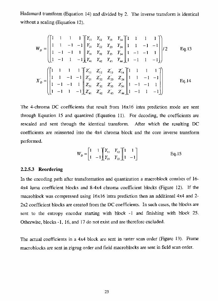
Hadamard transform (Equation 14) and divided by 2. The inverse transform is identical

without a scaling (Equation 12).

'

1 1 1 1

1 1 -1 -1

WD =

1 -1 -1 1

i1 -1 1 -1

'-\ 1 1 1"

*o =

1 1

1 -1

-1

-1

-1

1

1 -1 1 -1

122

'32

'42

"32

"42

23

l33

J23

"33

'34

'24

1 1 -1 -1

1 -1 -1 1

1 -1 1 -1

"1 1 1 1

1 1 -1 -1

1 -1 -1 1

1 -1 1 -1

12 Eq.13

Eq.14

-V

The 4-chroma DC coefficients that result from 16x16 intra prediction mode are sent

through Equation 15 and quantized (Equation 11). For decoding, the coefficients are

rescaled and sent through the identical transform. After which the resulting DC

coefficients are reinserted into the 4x4 chroma block and the core inverse transform

performed.

W =

1 1

1 IT YJL 21 '22.

1 1

1 -1

Eq.15

2.2.5.3 Reordering

In the encoding path after transformation and quantization a macroblock consists of 16-

4x4 luma coefficient blocks and 8-4x4 chroma coefficient blocks (Figure 12). If the

macroblock was compressed using 16x16 intra prediction then an additional 4x4 and 2-

2x2 coefficient blocks are created from the DC coefficients. In such cases, the blocks are

sent to the entropy encoder starting with block -1 and finishing with block 25.

Otherwise, blocks -1, 16, and 17 do not exist and are therefore excluded.

The actual coefficients in a 4x4 block are sent in raster scan order (Figure 13). Frame

macroblocks are sent in zigzag order and field macroblocks are sent in fieldscan order.

23

16

J

0

J

1

J

4

IT

5

J

2

J

3

J

6

J

7

J

8

J

9

J

12

J

13

J

10

J

11

J

14 15

Luma

3 lain E. G. Richardson

18 19

20 21

Cb

j,

22

J

23

id

24

J

25

Cr

Figure 12: 16x16 Macroblock BlockOrdering151

--2

12

13

14

-16

Zig-Zag Scan Field Scan

Figure 13: Raster ScanOrders for Decoding

2.2.6 Entropy Coding

Entropy coding techniques are aimed at compressing bit-level information. In the H.264

standard most header information is encoded usingfixed- and variable-length binary

codes and actual data encoded usingvariable-length codes (VLC) or context-adaptive

24

arithmetic coding (CABAC)[5]. CABAC is available in the main profile but excluded

from the Baseline Profile. For a reference on CABAC please refer to [5].

2.2.6.1 Variable Length Codes

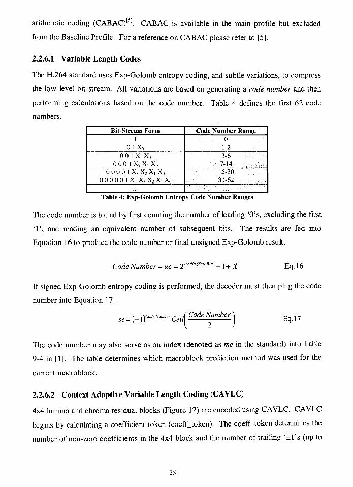
The H.264 standard uses Exp-Golomb entropy coding, and subtle variations, to compress

the low-level bit-stream. All variations are based on generating a code number and then

performing calculations based on the code number. Table 4 defines the first 62 code

numbers.

Bit-Stream Form Code Number Range

1

0 1X0

0

1-2

00 1 X, Xo

0 0 0 1 X2 X, X0

3-6

7-14

0 0 0 0 1 X3 X2 X, x0

0 0 0 0 0 1 X4 X3 X2 X, Xq

15-30

31-62

Table 4: Exp-Golomb Entropy Code Number Ranges

The code number is found by first counting the number of leading '0's, excluding the first

T, and reading an equivalent number of subsequent bits. The results are fed into

Equation 16 to produce the code number or final unsigned Exp-Golomb result.

CodeNumber=ue =2kadi"gZer"Bi's

-\ + X Eq.16

If signed Exp-Golomb entropy coding is performed, the decoder must then plug the code

number into Equation 17.

1 CodeNumber^

se =(-!)'Code Number

Ceil Eq.17

The code number may also serve as an index (denoted as me in the standard) into Table

9-4 in [1]. The table determines which macroblock prediction method was used for the

current macroblock.

2.2.6.2 Context Adaptive Variable Length Coding (CAVLC)

4x4 lumina and chroma residual blocks (Figure 12) are encoded using CAVLC. CAVLC

begins by calculating a coefficient token (coeffjoken). The coeffjoken determines the

number of non-zero coefficients in the 4x4 block and the number of trailing 'l's (up to

25

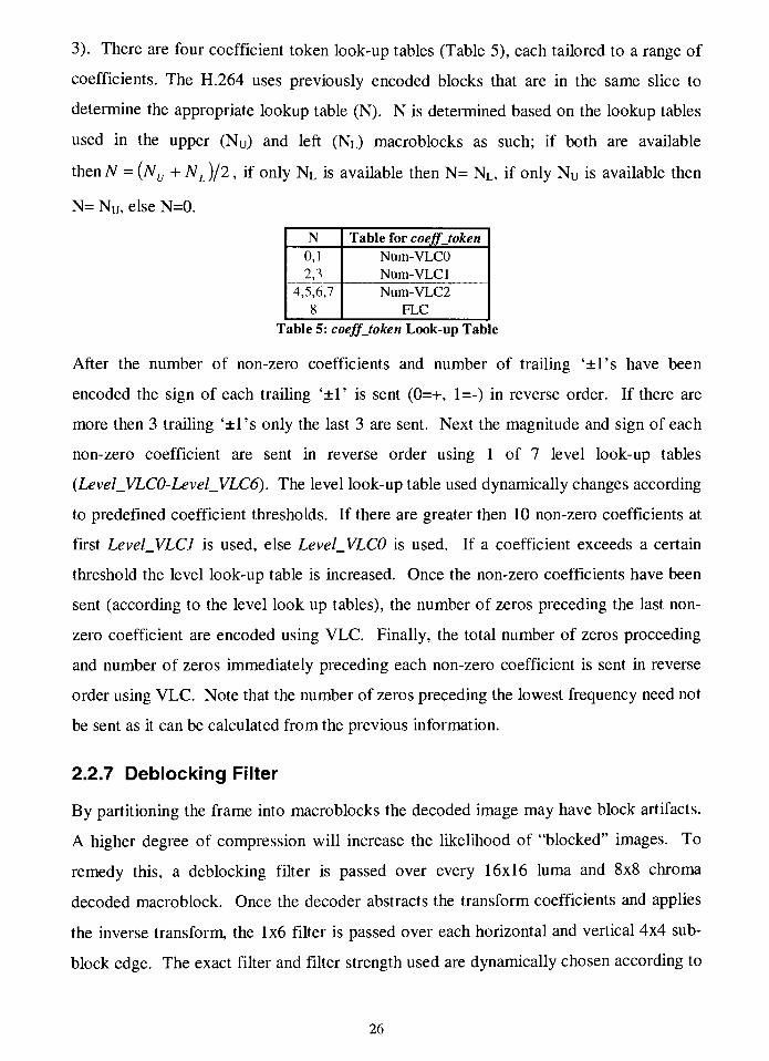
3). There are four coefficient token look-up tables (Table 5), each tailored to a range of

coefficients. The H.264 uses previously encoded blocks that are in the same slice to

determine the appropriate lookup table (N). N is determined based on the lookup tables

used in the upper (Nu) and left (NL) macroblocks as such; if both are available

thenN = (Nu + NL )/2 , if only NL is available then N= NL, if only Nu is available then

N= Nu, else N=0.

N Table for coeffjoken

0,1

2,3

Num-VLCO

Num-VLCl

4,5,6,7

8

Num-VLC2

FLC

Table 5: coeffjoken Look-up Table

After the number of non-zero coefficients and number of trailing 'l's have been

encoded the sign of each trailing'1'

is sent (0=+, 1=-) in reverse order. If there are

more then 3 trailing 'l's only the last 3 are sent. Next the magnitude and sign of each

non-zero coefficient are sent in reverse order using 1 of 7 level look-up tables

(Level_VLC0-Level_VLC6). The level look-up table used dynamically changes according

to predefined coefficient thresholds. If there are greater then 10 non-zero coefficients at

first Level_VLCl is used, else Level_VLC0 is used. If a coefficient exceeds a certain

threshold the level look-up table is increased. Once the non-zero coefficients have been

sent (according to the level look up tables), the number of zeros preceding the last non

zero coefficient are encoded using VLC. Finally, the total number of zeros proceeding

and number of zeros immediately preceding each non-zero coefficient is sent in reverse

order using VLC. Note that the number of zeros preceding the lowest frequency need not

be sent as it can be calculated from the previous information.

2.2.7 Deblocking Filter

By partitioning the frame into macroblocks the decoded image may have block artifacts.

A higher degree of compression will increase the likelihood of"blocked"

images. To

remedy this, a deblocking filter is passed over every 16x16 luma and 8x8 chroma

decoded macroblock. Once the decoder abstracts the transform coefficients and applies

the inverse transform, the 1x6 filter is passed over each horizontal and vertical 4x4sub-

block edge. The exact filter and filter strength used are dynamically chosen according to

26

the macroblock content and encoding method. For a detailed explanation of the

deblocking filter refer to [2].

2.3 MicroBlaze Soft-Processor

Xilinx has put together a development suite, known as the Embedded Development Kit

(EDK), which allows the user to turn an FPGA or portion of an FPGA into a processor.

In addition to the development environment, Xilinx provides a library of VHDL

Intellectual Property (IP) Modules to incorporate into the processor design. This type of

configurable VHDL implemented processor has been dubbed a soft-processor. Xilinx in

fact offers three separate soft-processor designs. They are, listed in increasing

complexity, PicoBlaze, MicroBlaze, and PowerPC. Although diverse, the PowerPC is a

bit large for decoding an H.264 bit-stream and would occupy a large amount of space on

the FPGA. The Picoblaze is directed at small applications with limited instruction

memory. For these reason the MicroBlaze processor has been chosen as the decoder

platform. MicroBlaze is able to address enough RAM to execute the code required and

uses fewer gates then the PowerPC. The following is a summarized description of the

MicroBlaze based on documentation provided by Xilinx.

2.3.1 Processor Architecture

TheMicroBlaze processor is a 32-bit load/store RISC processor. As with most load/store

architectures the MicroBlaze consists of a program counter, instruction decoder,

Arithmetic Logic Unit (ALU), and a bank of registers to execute the instruction set.

The soft-processor architecture also contains an instruction buffer to facilitate pipelining

and two memory interfaces (IF); one for data and one for instruction. A Machine Status

Register (MSR) tracks the current state of the processor and retains information from the

last executed instruction such as divide by zero (DBZ), Carry (C), Interrupt Enable (IE),

etc. The MicroBlaze also provides stack instructions and a stack pointer (SP) for ease of

use.

The ALU provides simple integer arithmetic and integer operations (shift, barrel shift,

etc). There is no hardware within the processor architecture to support floating point

27

(FP) instructions. This means that the compiler must break down any floating points and

FP operations into integer arithmetic algorithms that consume several instructions and

clock cycles. A programmer writing in a high level language must take into

consideration the latency introduced with the use of floating points. The register bank

consists of 34 32-bit registers (Table 6). Note that in reality the programmer only has full

reign over 23"free"

registers (R2-R12 and R19-R31). The remaining 9 registers are

dedicated to maintaining process flow. The"free"

registers are divided into two

categories, volatile and non-volatile. Volatile registers do not retain their value across

function calls while non-volatile register do. It is up to the programmer to push any

volatile registers on the stack prior to a function call.

Register Type Purpose

RO

RI

Dedicated

Dedicated

= 0

Stack Pointer

R2

R3-R4

Dedicated

Volatile

Read-only small data area anchor

Return Values

R5-R10

R11-R12

Volatile

Volatile

Passing parameters/Temporaries

Temporaries

R13

R14

Dedicated

Dedicated

Read-write small data area anchor

Return address for Interrupt

R15

R16

Dedicated

Dedicated

Return address for Sub-routine

Return address for TrapR17

R18

Dedicated

Dedicated

Return Address for Exception

Reserved for Assembler

R19-R31

RPC

Non-volatile

Special

Must be saved across function calls

Program Counter

RMSR Special Machine Status Register

Table 6: MicroBlaze Register Bank

2.3.1.1 Pipeline

The MicroBlaze architecture consists of 3-pipeline stages; fetch, decode, and execute.

Each stage may work on a concurrent instruction prior to the completion of the current

instruction. The processor assumes that every branch is not taken resulting in a 1 -cycle

penalty for branching. A 2-cyle penalty is avoided by allowing the instruction

immediately after the branch to execute.

2.3.1.2 Cache

The hardware designer has the option to include an instruction and data cache

(implemented via EDK). The cache is provided to optimize larger designs that require

28

external memory. Hereafter external memory refers to memory that is not located on-

chip with the FPGA while internal memory refers to the Block RAM (BRAM) that is

provided on-chip with the FPGA. The instruction and data cache reside in local memory.

In cache 2-bits are appended to signify whether an instruction or address is cacheable or

non-cacheable. In total memory may contain 1-GB of cacheable memory and 3-GB of

non-cacheable memory. An address in cache is divided into a tag address and cache line.

The cache line can be 9 to 14 bits yielding a 4kB to 64kB cache respectively. Every

instruction fetch is sent to cache and primary memory via the address bus. Primary

memory is located either in local memory, external memory, or a combination. If the

address is in non-cacheable memory then the cache ignores the fetch. Otherwise the

cache performs a tag look-up to see if the line is in cache, if so it returns the data. If the

data is not in cache then the processor must wait for primary memory to return.

2.3.2 Processor Busses

There are four busses available and compatible with the MicroBlaze soft-processor. One

of the busses provides access for high speed peripherals (FSL), another connects the

processor to local data and instruction memory (LMB), and the final two busses serve as

general access lines to both peripherals and external memory.

2.3.2.1 Fast Simplex Link (FSL)

The MicroBlaze has access to 8-master and 8-slave Fast Simplex Link Interfaces. The

FSL bus is implemented on the FPGA as a FIFO. Each FSL interface contains two 32-bit

wide buses, one for read and the other for write. The FSL is designed to provide access

to one way streaming data. Each interface contains a bit that specifies the direction of the

bus. An FSL interface allows the processor to directly communicate with peripherals

without sharing the data lines with other modules. This is very useful for signal

processing, image processing, network processing,etc.[14]

The FSL expedites

communication for high priority control and data acquisition. When multiple MicroBlaze

processors are placed on a single FPGA the FSL is typically used for inter-processor

communications.

29

2.3.2.2 LocalMemory Bus (LMB)

The LocalMemory Bus serves a single purpose, connecting the MicroBlaze to instruction

and data memory. Local memory is comprised of the Block RAM (BRAM) that resides

within the FPGA. It is up to the designer on how much memory to allocate to the

MicroBlaze. The EDK suite and compiler differentiate and control the actual

differentiation between instruction and data memory within each BRAM. The LMB is

designed to provide read and write access in a single clock cycle. If the designer chooses

to implement memory hierarchy using cache, the cache resides in local memory and

connects to the CPU via the LMB. The minutiae of the LMB are mostly abstracted from

the user.

2.3.2.3 Processor Local Bus (PLB)

The processor local bus is part of IBM'sCoreConnect

Bus architecture1141. The PLB is

designed to connect the processor to high speed peripherals such as network interfaces

and external memory. Concurrent read and write operations are supported by supplying

separate 64-bit data lines for each. The address line is fixed at 32-bits wide. The bus

controller uses an address pipeline to allow multiple requests prior to returned data

decreasing the average access time. Any number of slave devices may be connected to

the bus but only 16 master devices may be active. Each read/write may be associated

with a priority in order to further flexibility among master devices. 16, 32, and 64-byte

transfers are supported as well as Direct Memory Access (DMA) to relinquish the CPU

during transfer between devices. The PLB standard specifies dynamic bus sizing to allow

for 32 and 64-bit devices. This functionality is not supported by Xilinx and all

peripherals are assumed to be 64-bits wide. Since the MicroBlaze itself is a 32-bit

processor the designer must take particular care when connecting a module to the PLB.

Specifically for byte and half-work address access. A more detailed explanation of

connecting a device to aMicroBlaze processor via the PLB is in [14]. The PLB increases

bus performance at the cost of complexity. Xilinx does not supply any wrapper

templates to connect user defined VHDL modules to the PLB. However, Xilinx does

supply proprietary modules for 1 -Gigabit Ethernet, external memory, and DDR SRAM.

30

2.3.2.4 On-chip Peripheral Bus (OPB)

The On-chip Peripheral Bus is also part of IBM'sCoreConnect

bus structure. The

OPB consists of a single data bus eliminating the possibility of concurrent read and write

operations. Although the IBM OPB supports 32 and 64-bit wide data and address lines;

Xilinx only provides 32-bit functionality. The OPB is designed to simplify the

connection and protocol between peripherals and the CPU. All devices are memory

mapped with a minimum address span of 1024-bytes (assuming each address contains a

32-bit work). A 4-bit byte enable signal allows for byte, half-word, and word operations.

Any number of master and slave devices can be connected to the bus at one time as long

as the memory map does not exceed the address limits.

To expedite the development of user defined modules, Xilinx supplies a set of templates

and requirements to connect VHDL entities to the OPB. These templates are known as

Intellectual Property Interconnects (IPIC). It is the responsibility of the designer to

connect a user defined device to the IPIC and adhere to the bus the protocol. The IPIC is

further wrapped inside of an Intellectual Property Interface (IPIF). Within the IPIF lies

the logic that communicates with the OPB Arbiter, performs address decoding, and relays

pertinent signals to the IPIC. As the OPB and OPB Arbiter go through revisions and

evolve, it is the responsibility of the IPIB to adhere to the new protocol and abstract the

IPIC from the OPB. This ensures that any user module that connects through IPIC will

not require any changes with future revisions of the OPB. Figure 14 illustrates a typical

IPIC read and write sequence and lists the typical signals used to connect to the IPIC. All

signals are triggered off the rising edge of the bus clock (BusIPjClk).

31

Bus2IP_Clk

Bus2IP_Addr

Bus2IP_BE

Bus2IP Burst

Bus2IP_RNW

Bus2IP_CS(i)

Bus2IP_CE(i)

Bus2IP_RdCE(i)

Bus2IP_WrCE(i)

Bus2IP_Data

Bus2IP_Freeze

IP2Bus_0ata

IP2Bus_Ack

IP2Bus_Error

IP2Bus_Retry

IP2Bus_Toutsup

IP2Bus_lntr

IP2Bus_PostedWrlnh

Single Beat Read

Ao

Single BeatWrite

Ao

i

1 )11 !) X 1 m mA

1 1 1 1 1

:A~

^^1 1 1 i 1

1 1 1 t 1

\ / ~T^ : !\ :

:

r~

iV_ [y :\ :

; // i^

i

i i

i

i i V :\ !

i i i i i i i i >

i < i i i i i i

-I ! < 1 1 1 t 1 1 1-

/ iv_ i i / T\

i i

i i

i i

[ ]

i i

Xilinx

Figure 14: IPIC Bus Read and Write Sequence

2.3.3 Interrupts, Breaks, and Exceptions

The flow of the processor may be interrupted in three ways; interrupts, exceptions, and

breaks. Interrupts are enabled via the Interrupt Enable bit (IE) in the MSR. The MSR

also contains a Break in Progress bit (BIP) to state that the processor is executing code in

a break. When an interrupt occurs the code branches to address 0x00000010, subsequent

interrupts are blocked, and the return address is stored in R14. When an exception occurs

the return address is stored in R17 and the code branches to address 0x00000008. There

are two types of breaks, hardware and software. A software break may be invoked using

the BRK or BRKI instructions. In either case the return address is stored in the specified

register and the BIP is set high. If a hardware or external break is trigger the BIP is set

high, the return address is stored in R16, and the PC jumps to 0x00000018. Hardware

breaks are ignored if the BIP is high.

2.3.4 Kernel and Drivers

As with most processors it is preferable to program with a higher-level language then

assembly. Often a compiler can generate more efficient code and be programmed to

recognize mistakes that are overlooked in assembly. Fortunately the MicroBlaze has a C-

32

compiler and linker based on gcc. Another major advantage to the EDK suite and the

MicroBlaze soft-processor is that a minimal kernel can be loaded to build and run on top

of.

One of the main advantages of the kernel is the abstraction from memory management.

Xilinx provides calls similar to malloc and free ANSI C. Note that this implies dynamic

memory allocation. Xilinx also provides a set of standard C libraries to facilitate

development. Complete documentation is available in [13]. The main libraries of

interest are those that allow for dynamic memory allocation, standard I/O operations

(writing to memory), interrupt handling, and a file management. Data in memory may

now be placed in files and accessed through file pointers instead of tracking memory

locations. To further extend the functionality of the IP, EDK also contains a library of

API's to pair with their hardware counterparts. There is a complete socket interface to

build on top of the Ethernet module; printf statements automatically pipe stdout through

the UART.

For higher level programming the kernel contains system calls for process management,

thread management, semaphores, message queues, and shared memory. To expedite the

project turn around time and keep the design simple, the MicroBlaze will be limited to a

single process throughout the scope of the thesis. However, it is likely that a multi

process design will be beneficial in the future as additions are made to the design. The

XiLinx Micro Kernel includes real-time operations and can support the VxWorks and

MicroLinux Operating Systems.

33

3 HW/SW Hybrid H.264 Decoder Design

To expedite the development process of a hybrid decoder the inverse quantizer, inverse

transform, inter an intra prediction modules, and deblocking filter from [7] were to be

combined into a single hardware entity, the H.264 Decoder Core. Software handles

reading the bit-stream, entropy decoding, CAVLC, output of results, and has top level

control. It is possible to move the hardware software boundary to optimize performance,

portability, or simplicity of design. Decoding the bit-stream into coefficients in software

and decoding coefficients into frames of pixels in hardware is an attempt to divide the

decoder into highly sequential (software) and highly parallel (hardware) operations.

The goal of this thesis was to demonstrate a viable combined hardware software H.264

decoder. Late in the development of both the hardware and software designs,

MicroBlaze proved unable to process the bit-stream in a real-time (an explanation of

results may be found in Section 4.3). For this reason the H.264 Decoder Core was never

added to the system. The following section describes the overall software design, the

hardware design of the MicroBlaze system, and the proposed hardware design of the

H.264 Decoder.

The EDK provides a design environment for integrating software and hardware solutions.

Using EDK the overall decoder hardware architecture was laid out in a schematic form.

In doing so, all interconnection signals amongst Xilinx IP modules, including

MicroBlaze, and the user peripheral modules designed specifically for the H.264 decoder

are automatically generated. The actual bit-stream hardware module (Section 3.1.1) and

proposed H.264 Decoder module (Section 3.1.3) were designed in VHDL. The software

was written in C (Section 3.2) and the associated executable created using EDK's

compiler.

34

3.1 Hardware Architecture

io n

ao ~

o wc .

"5

Data Instruction

AVC

Decoder

Core

0PB_Relay

o 2.

S %

OPB

AVC File

Core

OPB_Relay

o 2.

LMB_IF_Cntl BRAM

D-LMB

LMB_IF_Cntl

-LMB

OPB_v20

Microblaze

(software)

LMB_v10

5 Stephen Joralemon

Figure 15: HW/SW Hybrid H.264 Decoder

The hardware architecture was kept simple to expedite the design, implementation, and

testing phases (Figure 15). The MicroBlaze uses the OPB to access the bit-stream,

decode the software generated coefficients, and provide a mean of output. The OPB is

the most extensible of the buses and provides fast integration and a simple

communication interface. All user defined peripherals (H.264 Decoder, AVC File

Interface, and OPB Relay) connect to the MicroBlaze as slaves through the OPB arbiter

(OPB_v20). It is the responsibility of the OPB arbiter to maintain the integrity of the bus.

There is no external memory used throughout the operation of the decoder. The

MicroBlaze uses local BRAM that is on-chip with the FPGA for data and instruction

memory. Depending on the target FPGA and frame size of the video it may be necessary

to include external memory in future designs. The LMB arbiter (LMB_vlO) connects

MicroBlaze to memory controllers (LMB_IF_Cntl) which in turn connect to the actual

BRAM. Once the BRAM is connected to the MicroBlaze, EDK abstracts memory

management from the user. The MicroBlaze soft-processor, OPB arbiter, LMB arbiter,

and BRAM controllers were all generated from the Xilinx library of IP modules. Each of

the modules was then connected using the Xilinx Platform Studio (XPS), a development

35

environment that is part of the EDK. Figure 16 is the XPS representation of the hardware

design. Table 7 lists the memory map structure for both the LMB and OPB. Note that

the OPB and LMB arbiters are contained within the MicroBlaze module. Two user-

defined modules, H.264 DecoderCore[7]

(Section 3.1.3) and AVC File Core (Section

3.1.1), were to be attached to the OPB via another user defined module, OPB Relay

(Section 3.1.2). Note again that the proposed H.264 Decoder design was not

implemented; however, the OPB Relay Module (connection interface) was left in the

design.

Stephen Joralemon

Figure 16: XPS HW/SW Hybrid Decoder Layout

Module Start Address End Address Description

LMB_vlO

LMB_vlO

0x00000000

0x00000000

OxOOOOFFFF

OxOOOOFFFF

Instruction Memory Controller

DataMemory Controller

OPB_Relay_0

OPB_Relay_l

OxFFFFOOOO OxFFFFOOFF

OxFFFFlOFF

Connect to AVC File Core

Connect to H.264 Decoder CoreOxFFFFlOOO

Table 7: SystemMemory Map

3.1.1 AVC File Interface Module (External)

In order to test the entire design, the decoder must have access to an encoded H.264 bit-

stream. Since actual hardware will not be implemented, using protocols such as Ethernet

or USB would require simulating such hardware and generating protocol compliant

36

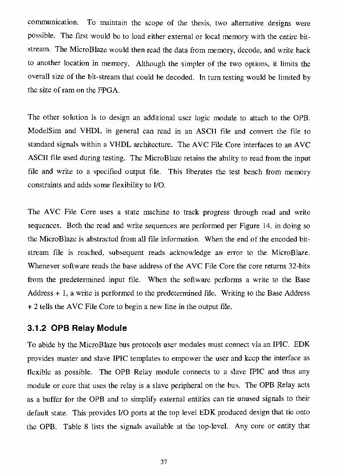
communication. To maintain the scope of the thesis, two alternative designs were

possible. The first would be to load either external or local memory with the entirebit-

stream. The MicroBlaze would then read the data from memory, decode, and write back

to another location in memory. Although the simpler of the two options, it limits the

overall size of the bit-stream that could be decoded. In turn testing would be limited by

the size of ram on the FPGA.

The other solution is to design an additional user logic module to attach to the OPB.

ModelSim and VHDL in general can read in an ASCII file and convert the file to

standard signals within a VHDL architecture. The AVC File Core interfaces to an AVC

ASCII file used during testing. The MicroBlaze retains the ability to read from the input

file and write to a specified output file. This liberates the test bench from memory

constraints and adds some flexibility to I/O.

The AVC File Core uses a state machine to track progress through read and write

sequences. Both the read and write sequences are performed per Figure 14, in doing so

the MicroBlaze is abstracted from all file information. When the end of the encoded bit-

stream file is reached, subsequent reads acknowledge an error to the MicroBlaze.

Whenever software reads the base address of the AVC File Core the core returns 32-bits

from the predetermined input file. When the software performs a write to the Base

Address + 1, a write is performed to the predetermined file. Writing to the Base Address

+ 2 tells the AVC File Core to begin a new line in the output file.

3.1.2 OPB Relay Module

To abide by the MicroBlaze bus protocols user modules must connect via an IPIC. EDK

provides master and slave IPIC templates to empower the user and keep the interface as

flexible as possible. The OPB Relay module connects to a slave IPIC and thus any

module or core that uses the relay is a slave peripheral on the bus. The OPB Relay acts

as a buffer for the OPB and to simplify external entities can tie unused signals tothen-

default state. This provides I/O ports at the top level EDK produced design that tie onto

the OPB. Table 8 lists the signals available at the top-level. Any core or entity that

37

connects to the OPB Relay Module must adhere to the OPB protocols[l5]. Two OPB

Relays are used for in the top level design. The first connects the AVC File Core to the

OPB; the second provides connection to a H.264 Decoder Core.

Port Direction Description

RELAY_OUT_Clk

RELAY_OUT_Rst

Out

Out

Bus clock

Bus reset, Active low

RELAY_OUT_ABus

RELAY_OUT_DBus

Out

Out

32-bit address bus

32-Bit Write data bus

RELAY_OUT_RdCE

RELAY_OUT_WrCE

Out

Out

Read chip enable

Write chip enable

RELAY_OUT_CS

RELAY_IN_DBus

Out

In

Chip select

32-Bit Read data bus

RELAY_IN_errAck

RELAY_IN_xferAck

In

In

Error after write

Acknowledge transfer (write)

RELAY_IN_retry

RELAY_IN_toutsup

In

In

Tell MicroBlaze to retry write

TypicallyMicroBlaze waits for the write acknowledge

signal for 8-cycles, toutsup forces to the MicroBlaze

to wait after a write until toutsup is low

Table 8: OPB Relay Signals

The main advantage of the OPB Relay Module is that it adds a level of detachment from

the MicroBlaze System Design. EDK allows a user to simulate a design using

ModelSim. Furthermore, the user can specify whether to generate behavioral or

structural modules of the MicroBlaze hardware. If any user modules are included in the

design that contain behavioral code, it limits the simulator to all behavioral descriptions.

Using the OPB Relay Module provides OPB I/O at the top level MicroBlaze System

Design. One can use EDK to generate structural hardware modules for simulation then

attach behavioral entities to the MicroBlaze via the OPB Relay Module. Designs may

now progress from un-synthesizable to synthesizable step by step all while simulating

with a structurally accurate MicroBlaze, OPB controllers, memory, LMB controllers, etc.

Note that using EDK the project may be exported to Project Navigator which, in turn,can

perform placement and routing. Since the top level MicroBlaze System Design would

have to be structural, behavioral modules can be tested with very accurate simulations of

theMicroBlaze running on an FGPA.

38

3.1.3 AVC Decoder Core

rn-1

(reference)

Encoded

Bit Stream

Microblaze

(Software) EntropyDecoder

AVC Decoder Core

(Hardware)

(reconstructed)

Stephen Joralemon

Figure 17: H.264 Decoder HW/SWDivision'71

As stated previously work has been done to design a H.264 decoder in VHDL[7]. It was

intended to use part of this design to expedite the development of the HW/SW Hybrid

Decoder. Unfortunately the MicroBlaze proved too slow to decode the bit-stream in real

time. For this reason the AVC Decoder Core was never actually integrated into the

system. The following section describes the preliminary design for future work. Figure 1

shows the divide between the software partitioning of the decoder and hardware portion.

The inverse quantizer, inverse transform, inter and intra prediction modules, and

deblocking filter were generated as part of [7]. These hardware modules can be

combined together with a top-level interface to create a AVC Decoder Core (Figure 17).

The H.264 Decoder Core takes 4x4 matrices of coefficients as input and returns

macroblocks of decoded pixels.

To connect the H.264 Decoder to an IPIC module and thus the OPB, a preliminary

interface was laid out. The interface consists of a bank of registers that store all of the

control data required by the H.264 Decoder Core. This control data is extracted from the

bit-stream by the software and stored into the registers. After all of the pertinent control

39

information has been set, the software can begin sending the 4x4 coefficient matrices

within a macroblock to the AVC Decoder Core. Another bank of registers, internal to the

AVC Decoder, is used to store each of the coefficient blocks. Once a 4x4 matrix is

written the software sets an enable bit high to trigger decoding of that sub-block. Table 9

breaks down in detail the preliminary address of each control register, the address of the

4x4 matrix bank, and the decode start address. All of the addresses represent an offset

from the base address assigned to the OPB Relay Core. After all of the 4x4 coefficient

blocks within a macroblock have been sent, the software attempts to read from the base

address of the AVC Decoder Core. In doing so the AVC Decoder Core sets the

RELAYJNjoutsup signal high until it has finished decoding the entire macroblock. This

signal blocks the MicroBlaze until the decoder is ready for the next matrix of coefficients

and provides that any subsequent reads to the decoder are valid (it's not busy).

Flexibility may be added by increasing the number of 4x4 coefficient register banks and

creating a FIFO buffer. When the buffer is full the MicroBlaze would block (using the

RELAY_INjoutsup line) else it writes all the 4x4 coefficients in the frame as fast as

possible. Once all 4x4 coefficient matrices have been written in a frame the MicroBlaze

could either perform a similar blocking read or respond to an interrupt.

40

Address Register Description

0x00 Control Status RegisterStatus information for decoder. Used to start a decode

sequence and signal decode finished.

0x01 NAL Reference IDC Specifies NAL content

0x02 NAL Unit Type Specifies data structure contained in NAL

0x03 Profde IDC Profile that bit-stream conforms to

0x03

0x04

Constraint Set Register

Level IDC

The 3-lsb bits specify constraint specifications

Profile level that bit-stream conforms to

0x05

0x06

Sequence Parameter Set ID

Log 2 Max Frame Number

Minus 4

ID associated with current Sequence Set

Used to calculate the number of frames in the sequence

0x07

0x08

Picture Order Count Type Specifies how to decode picture order

Log 2 Max Picture Order Count

LSB Minus 4Used in decoding process for picture order count

0x09

OxOA

Number ofReference Frames

Gaps in Frame Flag

Number of reference frames to keepAllows for gaps in decoding order

OxOB

OxOC

PictureWidth in Macroblocks

Minus 1

Picture Height in Map Units

Minus 1

Width of frame in Macroblocks

Height of frame in map units

OxOD Frame Flags Contains frame flags

0x10 Picture Parameter Set ID ID Associated with current Picture Parameter Set

0x11

0x12

Sequence Parameter Set ID

Picture Parameter Flags

Sequence Set that the picture set belongs to

Contains parameter flags

0x13

0x14

Number Slice of Slice Groups

Minus 1

Slice Group Map Type

Number of slice groups in frame

Specifies mapping of slice groups

0x15

0x16

Number ofReference IDX 10

Minus 1

Number ofReference IDX 1 1

Minus 1

Maximum reference index for reference index 0

Maximum reference index for reference index 1

0x17

0x18

Picture Init. QPMinus 26

Picture Init QS Minus 26

Initial value of Slice QPy for each slice

Initial value of Slice QSy for each slice

0x19 Chroma QP Index Offset Offset that shall be added to QPy and QSy0x2 0 Slice Flag Register Contains field picture flag0x21

0x22

First Macroblock in Slice

Slice Type

Address of first macroblock in current slice

Specifies slice type

0x23

0x24

Picture Parameter Set ID

Frame Number

Picture parameter set that slice belongs to

Frame that slice belongs to

Identifies IDR picture

Specifies the picture order count modulo

0x25

0x2 6

IDR Picture ID

Picture Order Count LSB

0x27 Slice QP Delta Initial value ofQPy

0X30-3F 4x4 Block ofCoefficients

0x4 0 Inter Prediction Mode Inter prediction mode used for 4x4 Coeff. Block

0x5 0 Intra Prediction Mode Intra prediction mode used for 4x4 Coeff. Block

Table 9: Hardware Address Table for the H.264 Decoder Core

41

3.2 Software Architecture

From here out the software portion of the SW/HW Hybrid Decoder will be referred to as

the Bit-Stream Decoder. It is the responsibility of the software (Bit-Stream Decoder) to

read in the encoded bit-stream from the AVC File Core and perform entropy and CAVLC

decoding. In doing so, the software extracts control information from the bit-stream as

well as prediction vectors and 4x4 coefficient blocks. Extracting the coefficient blocks is

the last step prior inverse quantization thus the AVC Decoder Core. It is the

responsibility of the software to write all of the video header information, motion vectors,

prediction modes, and coefficients to banks of registers in the AVC Decoder Core. After

all of the coefficients in a macroblock have been sent to the decoder the software

performs a blocking read. Upon return the pixel data is read for that macroblock.

3.2.1 Software Design Process

Originally the software was to be an object oriented program writing in C++ providing

some rudimentary drivers to access the AVC File interface and AVC Decoder. However,

as coding progressed the inter dependability between classes and more importantly

between member functions grew. Throughout bit-stream extraction the software must be

fully aware of all data, states, and paths of previous. For this reason the software

architecture was changed into a strictly C-program in which all decoder data is globally

accessible. Although risks to data integrity increase, parameter passing and

dereferencing is greatly reduced.

The first revision of software targeted the PC as the application platform. The PC offers

more sophisticated and user friendly debugging tools. Error messages can be written to

screen during development as well to a file. Note that if actual hardware was available

and libraries loaded with the MicroBlaze, the software could also print to screen from the

FPGA. However, this is not possible during simulation. The same ASCII file

representations of encoded data were used as input. Once the software was running

satisfactory on the PC, it was migrated to the MicroBlaze platform. To ease this

migration pre-processor branch statements were added prior to any code that is specific to

either the PC or MicroBlaze. If one wishes to change the platform, only a single define

42

statement needs to be changed. Specifically if the macro MICROBLAZE is defined then

the target platform is the MicroBlaze soft-processor, else it is the PC. All code is

contained within a single c-file (main.c) and header-file (globals.h).

To debug during simulation, statements were added that put error codes onto the OPB

data lines. This permitted process flow to be mapped during simulation. Some

difficulties arose when the software was migrated to the MicroBlaze soft-processor. The

software appeared to be entering infinite loops at sporadic points within the code. It was

found that the stack size was insufficient to contain such a large program. By default the

stack size is set to 0x3FF, to prevent any overflow the stack size was ultimately set to

0x2FFF.

3.2.2 Top Level Functionality

The MicroBlaze immediately begins executing the Bit-Stream Decoder after startup.

Upon execution the software allocates space for all global variables and data structures.

After initialization the bit-stream is read in until a startjzodejprefix is found within the

bit-stream. This delimiter synchronizes the decoder and signals the start of a sequence

parameter set, a picture parameter set, or a slice. Accordingly one of three functions is

called; seqjparameter_setjrbsp, picjjarameter_setj~bsp, and sliceJ.ayer_without_

partitioningj-bsp. [1] dedicates an entire chapter (Ch. 7) to laying out pseudo-code for

an H.264 decoder. When possible, the naming conventions were kept to increase the

software legibility. By adhering to the pseudo code, the documentation within [1]

becomes easily applicable. For in depth software descriptions please refer to [1] as well

as the code for commenting.

Originally two drivers were to be written; one controlling the H.264 Decoder Core and

one providing AVC File I/O. However, due to the simplicity of interfacing with each of

the components it was decided to write in the low-level code directly with the Bit-Stream

Decoder. Both the AVC File Core and H.264 Decoder Core connect to the MicroBlaze

through the OPB. Since the OPB is memory mapped the modules are accessed through

43

Xilinx library function calls. In particular Xgpio_mSetDataReg and

Xgpio_mGetDataReg are used through out the code.

3.2.3 Reading the Bit-Stream

The bit-stream was read in 32-bits at a time into a 64-bit buffer. The buffer was

automatically filled after the software consumed the first 32-bits. All reads occurred

through the memory mapped AVC File Module at address OxFFFFOOOO. Writes were

performed using the same module and writing to address OxFFFFOOOl and 0xFFFF0002.

The former address implies a direct write to the output file while the later allows the

software to signal the start of a new line. Allowing file output capabilities provided a

means to verify prediction mode and coefficient values. This software may also be used

in the future to output actual pixel values.

Performing CAVLC on the bit-stream proved to require a greater degree of data storage

and processing than originally anticipated. To simplify the software certain assumptions

were made about the video stream to be decoded. These assumptions are as follows:

? The bit-stream conforms to the Baseline Profile specified in [1]

? There is a single slice within the image

The software must generate an address mapping to specify what slice and slice

group each macroblock belongs to. If there is ony one slice, the mappings

become trivial.

r A slice is contained within a single NAL unit

Typically a slice my be split across up to 4 NAL units. Assuming that a slice is

always sent within the same NAL unit simplifies the control structure of the

software. Fewer states are required to track a decoded slice.

? The pic_order_cntjype is always 0

pic_order_cnt_type specifies the order of the current frame and/or field being

decoded. By assuming that pic_order_cnt_type is always zero means that frames

and fields are sent in temporal order.

A data structure was created to store the number of non-zero coefficients in each 4x4sub-

block. Due to the afore mentioned assumptions the software can easily check the state of

44

the 4x4 coefficient block above and to the left and determine whether it is in the same

slice and the number of non-zero coefficients. Please refer to section 2.2.6.2 for a

reference on CAVLC decoding.

The H.264 standard provides 5 look-up tables containing variable length codes that are

used to decode the number of non-zero coefficients in a 4x4 sub-block, the number of

trailing ones in a 4x4 sub-block, the number of zero coefficients left to decode in a 4x4

sub-block, and the number of zeros before the next non-zero coefficient in a 4x4 sub-

block. The tables may be found in [1] section 9.2. The Bit-Stream Decoder software

uses two arrays to store the tables; the first contains the variable code length; the second

contains the variable code value. While reading the bit-stream the software looks at

mutual locations within each array. If both the length and value match to the current

code then the corresponding indices represent the decoded values. This entire process is

performed every time a bit is read, if no match is found, the next bit is read and the

process repeated. This method of decoding was used in the referencesoftware1'91

and

ported into the Bit-Stream Decoder Software.

3.2.4 AVC Decoder Core Interface

The following is a brief overview of the proposed AVC Decoder Core software interface.

Table 7 proposes the memory mapped structure containing all decoder control

information. This information would be written directly after a sequence parameter set,

picture parameter set, or slice header are parsed from the bit-stream. The coefficients are

abstracted from the bit-stream in 4x4 blocks. Once an entire macroblock is read (16-

luma sub-blocks and 8-chroma sub-blocks) each sub-block would be written to the

decoder one row at a time (4-coefficients). After the final coefficient is written, the

software would call a blocking read to the AVC Decoder Core. Once the read returns it

signals the decoder is finished and the subsequent 384-pixels may be read. For improved

performance input and output buffers could be added to overlap reads with the wait time

after a macroblock is sent to the AVC Decoder Core.

45

4 Test Bench and Results

4.1 Encoded Bit-Stream

The encoded bit-stream was generated using reference software[l9]. A configuration file

was used to ensure that the encoder adhered to the Baseline Profile as well as adhering to

the constraints outlined in section 3.2.3. Since the reference software outputs a binary

file, additional software was used to convert the binary file into an ASCII file consisting

of hexadecimal characters. This conversion software was provided as part of [7].

Converting the data into a hexadecimal ASCII file allowed for direct access from VHDL

code.

The reference software also produced a trace file that outlined the bit-stream that was

generated during encoding. This trace file lists in detail the sequence parameter set,

picture parameter set, slice header, and slice data information that is created. It also gives

the prediction mode, number of non-zero coefficients, and trailing ones for each 4x4

coefficient block.

4.2 Feeding the Decoder

The bit-stream is accessed by the decoder via VHDL module that reads a file local to the

simulation PC. These reads can only be simulated using a behavioral model; however, it

is necessary to perform a post place and route simulation for the entire system. A post

place and route simulation models the actual layout of the FPGA and net lists. It is the

most accurate design verification without actually running on hardware. In order to

simulate the hardware post place and route while providing file access the MicroBlaze

system was enclosed and placed into a higher level design (Figure 18 ). It is included in

the system test bench figure to specify where it would lie during simulation. Entities

outside of the MicroBlaze System Design are connected to the MicroBlaze using the

synthesizable OPB Relay Modules. The system clock and reset are generated using

behavioral code since they are outside of the MicroBlaze System Design. The test bench

was run in three steps to test the relay hardware and Bit-Stream Decoder (software).

46

System Test Bench

E

S

| CO

m

Microblaze System Design

RST

CLK

JUT.

AVC

Decoder

Core

A

rv/

AVC File

Core

Data Instruction

BRAMLMB_IF_Cntl - LMBJF_Cntl

OPB_Relay

o 2.

OPB

OPB_Relay

o

D-LMB -LMB

*LMB_v10

OPB_v20

Microblaze

LMB_v10

Stephen Joralemon

Figure 18: HW/SW Hybrid H.264 Decoder Test Bench

The initial run used entirely behavioral descriptions of the MicroBlaze soft-processor and

hardware modules. A small and simple program was written to read in from file and write

to file using the AVC File Core. The Xilinx EDK generates all the necessary VHDL

files, builds a script to compile all the necessary VHDL code and loads all the necessary

libraries for simulation with ModelSim. Small changes were made to the VHDL files

and scripts to incorporate the AVC File core and include the MicroBlaze System Design

as a component of the top level System Test Bench. The design was successfully

simulated using ModelSim 6.0a.

The second run used EDK to produce structural descriptions of the MicroBlaze soft-

processor and hardware modules. This project was then exported toXilinx'

s Project

Navigator 6.3. Problems arose loading the executable code into memory using Project

Navigator. Ultimately the .bmm file that was loaded by EDK into Project Navigator had

to be replaced with the .ucf file generated during the export. The design was compiled,

translated, and an FPGA mapping generated in Project Navigator. A test bench file was

then created using Project Navigator that conformed to Figure18. Modelsim was used to

perform the post translate and route simulation. Once again a simple program was used

47

to test functionality. The system clock was set to 100MHz as per Xilinx documentation

[18]. The simulation was successful and typical hardware phenomena were observed

such as signal skew and signal bouncing. As expected, since the MicroBlaze is a

synchronous digital system the structural software execution time did not differ from the

behavioral simulations. This verified that the code would execute in the same manner

during a behavioral simulation as during a structural simulation. Thus to avoid

unmanageable simulation times, behavioral descriptions were used for the final design.

The final simulation was laid out per Figure 18 without the H.264 Decoder Core.

Behavioral descriptions were used for the MicroBlaze soft-processor and corresponding

hardware entities. A bit-stream was generated using the reference software that consisted

of 3 frames. The Bit-Stream Decoder successfully decoded the prediction modes and

coefficients from the video stream. It is here that the MicroBlaze soft-processor proved

too slow for a real-time application. For this reason simulations were never run with the

H.264 Decoder Core. In order to identify bottlenecks additional code was added to track

the process flow. See the following section for results.

4.3 Results

The following section lays out the findings from simulation. The Bit-Stream Decoder

software was run on a behavioral description of the MicroBlaze hardware. The bit-

stream used consisted of a 3-frame video stream that was 176 x 144 pixels, QCIF (Table

1). To decode all header information, prediction modes, and coefficients prior to inverse

quantization took an average of 94ms. This does not include inverse quantization,

inverse transform, or prediction. The MicroBlaze soft-processor and software would

have to see a speedup of roughly 2.8x. In order to identify bottlenecks within the

software, function entrance and exit debug messages were added. Each message writes a

unique 8-digit hexadecimal number to the OPB in order to identify where in the software

the MicroBlaze is and when. The OPB data bus signal was written to a listing file using

ModelSim and evaluated accordingly. Table 10 breaks down the function calling tree in

the software. Rudimentary statistics were found (Table 11) to profile the code and

determine where, if any, improvements would have to occur to reach real-time.

48

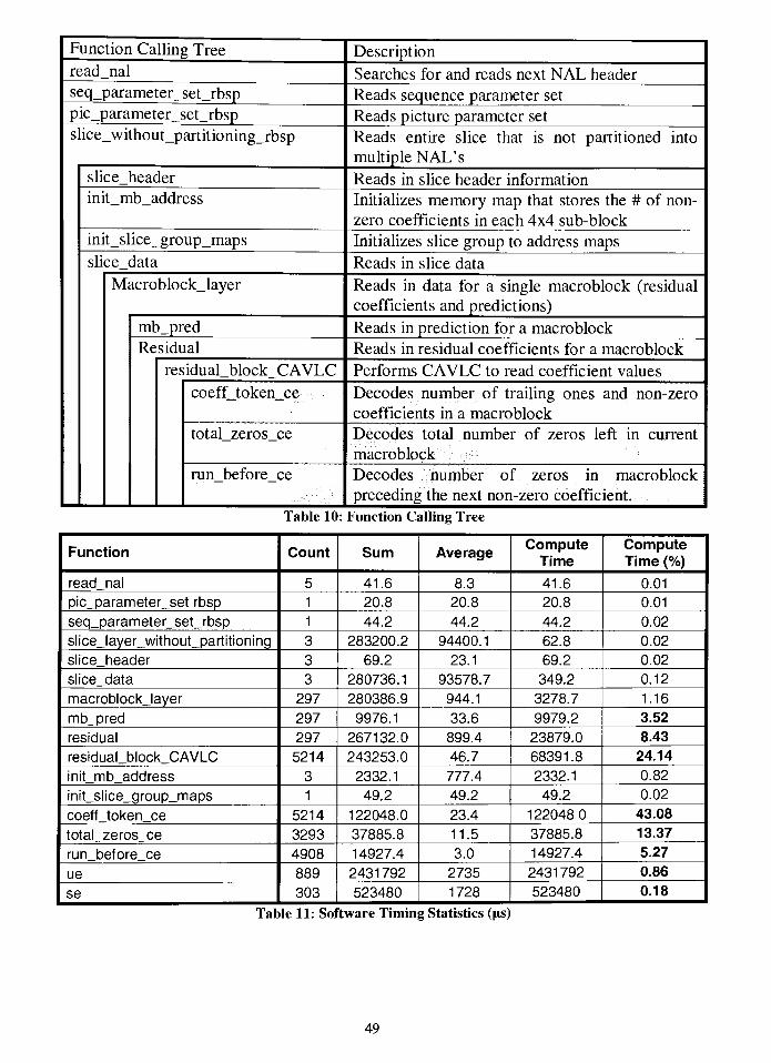
Function Calling Tree Description

read_nal Searches for and reads next NAL header

seq_parameter_set_rbsp Reads sequence parameter set

pic_parameter_set_rbsp Reads picture parameter set

slice_without_partitioning_rbsp Reads entire slice that is not partitioned into

multiple NAL's

slice_header Reads in slice header information

init_mb_address Initializes memory map that stores the # of non

zero coefficients in each 4x4 sub-block

init_slice_group_maps Initializes slice group to address maps

slice_data Reads in slice data

Macroblock_layer Reads in data for a single macroblock (residual

coefficients and predictions)

mb_pred Reads in prediction for a macroblock jResidual Reads in residual coefficients for a macroblock

residual_block_CAVLC Performs CAVLC to read coefficient values

coeff_token_ce Decodes number of trailing ones and non-zero

coefficients in a macroblock

total_zeros_ce Decodes total number of zeros left in current

macroblock

run_before_ce Decodes number of zeros in macroblock

preceding the next non-zero coefficient.

Table 10 : Function Calling Tree

Function Count Sum AverageCompute

Time

Compute

Time (%)

read nal 5 41.6 8.3 41.6 0.01

pic_parameter_set rbsp 1 20.8 20.8 20.8 0.01

seq_parameter_set_rbsp 1 44.2 44.2 44.2 0.02 i

slice_layer_without_partitioning 3 283200.2 94400.1 62.8 0.02

slice header 3 69.2 23.1 69.2 0.02

slice data 3 280736.1 93578.7 349.2 0.12

macroblockjayer 297 280386.9 944.1 3278.7 1.16

mb_pred 297 9976.1 33.6 9979.2 3.52

residual 297 267132.0 899.4 23879.0 8.43

residual block CAVLC 5214 243253.0 46.7 68391.8 24.14

init mb address 3 2332.1 777.4 2332.1 0.82

init_slice_group_maps 1 49.2 49.2 49.2 0.02

coeff token ce 5214 122048.0 23.4 122048.0 43.08

total zeros ce 3293 37885.8 11.5 37885.8 13.37 |run before ce 4908 14927.4 3.0 14927.4 5.27

ue 889 2431792 2735 2431792 0.86

se 303 523480 1728 523480 0.18

Table 11: Software Timing Statistics (jus)

49

The Sum represents the total amount of time that was spent in each function including its

underlying functions. The Compute Time represents the amount of actual computation

time spent in each function. This does not include time spent in underlying functions.

The Compute Time (%) is used to identify where the software spends the majority of

time. The bottom five functions in Table 10 are of particular interest.

The function initjnbjaddess is run once a frame and is responsible for initializing a

block of memory that holds the number of non-zero coefficients in every 4x4 coefficient

block. Stepping through every memory address is very time consuming for the

MicroBlaze and takes an average of 777us per frame. The other four functions,

residualjblockjCAVLC, coeff_token_ce, total_zerosj:e, and runjbeforejce, may run

multiple times for each macroblock that is decoded and occupy 85% of the computation

time. Thus any small improvement in these functions could result in a large overall

decrease in execution time.

50

5 Conclusion

Improvements in the system design must be pursued in order to decode the bit-stream in

real-time. It took roughly 94ms to perform all run length and entropy decoding on a

single QCIF frame. To approach real-time processing a software speedup of at least 2.8x

will have to be achieved. The majority of the computation time was spent performing

CAVLC decoding (>85%). Alternative CAVLC decoding techniques would result in

significant speed-up. It would also be beneficial to implement an I/O buffering scheme

to handle the bit stream and low-level entropy decoding. The EDK also provides the

ability to specify the cache configuration that is incorporated with the MicroBlaze

instantiation. It may be possible to improve performance by adding and testing different

cache configurations.

5.1 Future Work

A major advantage ofXilinx'

s EDK is the ease at which software and hardware units

may be interchanged. This allows a problem to be tackled first in software to expedite

the design process. Once a viable solution is found, bottlenecks can be identified and

functionality transferred to hardware modules directed at increasing performance. It is in

this manner that future work with the HW/SW hybrid H.264 decoder should take place.

The majority of the computation time was spent performing CAVLC decoding (>85%).

Several times per macroblock the software must search through multi-dimensional

lookup tables. Improvements in these functions would result in significant speed-up. It

would also be beneficial to implement a buffering scheme in I/O to handle the bit stream

and low-level entropy decoding. Buffering is currently done in the software for

simplicity during simulations.

Figure 16 specifies a new hybrid decoder layout reflecting possible changes to the

hardware architecture. The AVC File Core is replaced with a Buffer Core that handles

buffering and low-level Exp-Golomb Coding. An additional module is added to perform

CAVLC and has direct access to the bit-stream through the Buffer Core (Figure 19).

51

si

| CO

m

AVC

Decoder

Core

IQ

IT

Pred

Data Instruction

CAVLC

Core

LookupTables

-N

V

Buffer

Core

Buffer

Exp-

Golomb

LMB_IF_Cntl BRAM

D-LMB

- LMB_IF_Cntl

-LMB

*~LMB_v10

OPB

OPB_v20

MicroBlaze

(software)

LMB v10

Stephen Joralemon

Figure 19: Proposed Hardware Design

5.1.1 CAVLC Core

A major bottleneck in the software is performing Context Adaptive Variable Length

decoding in order to abstract residual coefficients from the bit-stream. This includes

residual_block_CAVLC,coeff_token_ce, totaljzeros_ce, and run_before_ce (see Table

10). residual_block_CAVLC is run for almost every single 4x4 sub-block and must first

calculate the number of non-zero coefficients in adjacent sub-blocks. If the adjacent

blocks are not decoded or not in the same slice then they are considered not available.

This process consumes roughly 24% of the computation time, residual

then calls coeffjoken_ce, total_zeros_ce, and runjbeforejzt. It is here that CAVLC is

actually performed and 62% of total execution time spent. The H.264 standard provides

a series of lookup tables that contain the actual variable length codes. In order to decode

the stream, all of these tables must be stored in memory and readily accessible. The

software reads a single bit at a time from the video stream, tracking the number of bits

read thus far and the code produced. After each bit is read an exact match for the current

code and length is searched for in the lookup tables, if none is found then the subsequent

bit is read and the lookup process repeated.

52

To reduce the computation time spent cycling through the lookup tables and the software

memory required to store the tables, the entire process could be put into a hardware

lookup table (LUT) module (Figure 20).

pBlaze

CAVLC Core

Control Unit

nC I length | code trail 1's # non-zero

Stephen Joralemon

Figure 20: CAVLC Core

Here three keys would be used to index into the LUT's. The first key, nC, is found in

software as a result of the adjacent sub-blocks. The length represents the number of bits

in the current bit-sequence to be decoded. The code key is the actual value given by the

bits read thus far. The LUT would return the two indexed values representing the number

of non-zero coefficients and trailing ones in the current sub-block. Providing a LUT for

coeff_token_ce, total_zerosjce, and runjbeforejze could greatly reduce computation

time.

For further speedup the CAVLC LUT's could be wrapped into a hardware core that

would attach directly to a Buffer Core (see Section 5.1.2). In doing so, the software

would no longer read 1-bit at a time and then index into a LUT. MicroBlaze would

simply read from a CAVLC Core which would in turn read from the Buffer Core

automatically and search through the LUT until a match was found (Figure 20). If the

53

I/O and Buffer Core were fast enough, it would now require a single read to perform

CAVLC. Theoretically with 3-clock cycle read (Figure 14), this would result in an

overall speed-up of 2.6, or 27.6 frames/sec.

5.1.2 Buffer Core

Processing the bit stream at a low-level is highly dependent upon the hardware that is

used to transmit the data. Foremost, the hardware has a direct effect on the buffer scheme

that would yield the fastest decode times. In any case, it would be beneficial to

implement not only an I/O buffer in hardware but also provide some of the low-level

decoding in hardware.

Exp-Golomb-coded syntax elements (see Section 2.2.6.1) are used frequently throughout

the standard[,]and require a loop in software to count and read the bit stream a single bit

at a time for up to 17 bits. It would not require a significant amount of gates to move this

low-level decoding to hardware. Ideally a single hardware module would handle both

buffering and low-level Exp-Golomb-decoding. Depending on the means used to acquire

the video stream (ethernet, disk drive, etc.) a Buffer Controller would handle low-level

communications and managing the actual FIFO buffer. Directly connected to the buffer

would be an array of addressable read/decode modules. MicroBlaze would read from a

given module based on the desired method of decoding. For example, if MicroBlaze

needed to perform unsigned Exp-Golomb decoding, then it would read from the

respective module within the Buffer Core (see Figure 21).

54

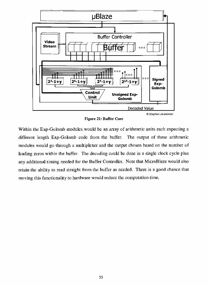
pBlaze

Video

Stream

Buffer Controller

^ffejr

X

23-l+y 25-l+y 27-l+y 2"-l+y

Ii

=n!fi=

A Control

J~

Unit

=L=

Unsigned Exp-

Golomb

Signed

Exp-

Golomb

Decoded Value

Stephen Joralemon

Figure 21: Buffer Core

Within the Exp-Golomb modules would be an array of arithmetic units each expecting a

different length Exp-Golomb code from the buffer. The output of these arithmetic

modules would go through a multiplexer and the output chosen based on the number of

leading zeros within the buffer. The decoding could be done in a single clock cycle plus

any additional timing needed for the Buffer Controller. Note that MicroBlaze would also

retain the ability to read straight from the buffer as needed. There is a good chance that

moving this functionality to hardware would reduce the computation time.

55

Bibliography

[1] ITU, Telecommunication Standardization Sector, "ITU-T Recommendation

H.264", ITU-T, May, 2003.

[2] Richardson, Iain E. G., H.264 and MPEG-4 Video Compression, 1 ed., The Atrium,Southern Gate, Chichester, West Sussex P019 8Sq, England: John Wiley & Sons

Ltd., 2003.

[3] Richardson, Iain E. G., "H.264 Intra Prediction", http://www.codex.com/h264.html,April, 2003.

[4] Richardson, Iain E. G., "H.264 Inter Prediction", http://www.codex.com/h264.html,

April, 2003.

[5] Richardson, Iain E. G., "H.264 Transform", http://www.codex.eom/h.264.html,

March, 2003.

[6] Gonzalez, Rafael C, Woods, Richard E., Digital Image Processing, 2 ed., Upper

Saddle River, New Jersey 07458: Prentice-Hall Inc., 2002.

[7] Warsaw, T., "VHDL Modeling and Synthesis of an H.264 Video Decoder", Thesis

Draft, March 2005.

[8] Wiegand T., Sullivan G., Bjontegaard G., Lutrha A.: "Overview of the H.264/AVC

Video Coding Standard", IEEE Transactions on Circuits and Systems for Video

Technology, July 2003.

[9] Hong, B., "Introduction to H.264", Multimedia Communications Laboratory,

University ofTexas, Nov. 22, 2002.

[10] Sentivision K.K., "Sentivision::Products::H.264::Overview",

http://www.sentivision.com/products/h264/h264-en.html. Copyright 2003-2005.

[11] Ittiam Systems (P) Ltd., "H.264", http://www.ittiam.com/pages/products/h264-

dec.htm.

[12] Ateme Ltd., "ATEME - H.264 /MPEG-4 AVC - DSP decoder",

http://www.ateme.com/products/h264 2.php, Copyright 2004.

[13] Xilinx Inc., "Embedded System Tools Guide", EDK (v3.2.2), May 21, 2003.

[14] Xilinx Inc., "MicroBlaze Processor Reference Guide", EDK (v3.2) April 1, 2003.

[15] Xilinx Inc., "User Core Templates Reference Guide", April 2003.

[16] Xilinx Inc., "Xilinx Device Drivers Documentation", May 29, 2003.

[17] Xilinx Inc., "Processor IP User Guide", June 2003.

[18] Xilinx Inc., "MicroBlaze the Industry's Fastest Soft Processor Solution for

FPGAs", 2003.

[19] Telenor Broadband Services, Ericsson Radio Systems, TELES AG, Nokia Inc.,

Nokia Corporation, Siemens AG, Heinrich-Hertz-Institute for Communication

Technology GmbH, University of Hannover, Institute of Communication Theoryand Signal Processing, Videolocus, Motorola Inc., Microsoft Corp., Apple

Computer Inc., RealNetworks Inc., Thomson Inc., "H.26L TML coder/decoder",

Copyright 2000.

Hardware Software Synthesis of a H.264 / AVC Baseline ...

Documents

Transcript of Hardware Software Synthesis of a H.264 / AVC Baseline ...