Accepted Manuscript

Content adaptive fast motion estimation based on spatio-temporal homogeneity

analysis and motion classification

Humaira Nisar, Aamir Saeed Malik, Tae-Sun Choi

PII: S0167-8655(11)00288-1

DOI: 10.1016/j.patrec.2011.09.015

Reference: PATREC 5230

To appear in: Pattern Recognition Letters

Received Date: 9 November 2009

Please cite this article as: Nisar, H., Malik, A.S., Choi, T-S., Content adaptive fast motion estimation based on spatio-

temporal homogeneity analysis and motion classification, Pattern Recognition Letters (2011), doi: 10.1016/j.patrec.

2011.09.015

This is a PDF file of an unedited manuscript that has been accepted for publication. As a service to our customers

we are providing this early version of the manuscript. The manuscript will undergo copyediting, typesetting, and

review of the resulting proof before it is published in its final form. Please note that during the production process

errors may be discovered which could affect the content, and all legal disclaimers that apply to the journal pertain.

1

Content adaptive fast motion estimation based on spatio-temporal 1

homogeneity analysis and motion classification 2

*1Humaira Nisar, 2Aamir Saeed Malik and 3Tae-Sun Choi 3 1Universiti Tunku Abdul Rahman, Perak, Malaysia 4

2Universiti Teknologi Petronas, Malaysia 5 3Gwangju Institute of Science and Technology, Korea 6

*Corresponding author: humaira@utar.edu.my 7

8

Abstract 9

In video coding, research is focused on the development of fast motion estimation (ME) 10

algorithms while keeping the coding distortion as small as possible. It has been observed that 11

the real world video sequences exhibit a wide range of motion content, from uniform to 12

random, therefore if the motion characteristics of video sequences are taken into account 13

before hand, it is possible to develop a robust motion estimation algorithm that is suitable for 14

all kinds of video sequences. This is the basis of the proposed algorithm. The proposed 15

algorithm involves a multistage approach that includes motion vector prediction and motion 16

classification using the characteristics of video sequences. In the first step, spatio-temporal 17

correlation has been used for initial search centre prediction. This strategy decreases the 18

effect of unimodal error surface assumption and it also moves the search closer to the global 19

minimum hence increasing the computation speed. Secondly, the homogeneity analysis helps 20

to identify smooth and random motion. Thirdly, global minimum prediction based on 21

unimodal error surface assumption helps to identify the proximity of global minimum. 22

Fourthly, adaptive search pattern selection takes into account various types of motion content 23

by dynamically switching between stationary, center biased and, uniform search patterns. 24

Finally, the early termination of the search process is adaptive and is based on the 25

homogeneity between the neighboring blocks. 26

Extensive simulation results for several video sequences affirm the effectiveness of the 27

2

proposed algorithm. The self-tuning property enables the algorithm to perform well for 28

several types of benchmark sequences, yielding better video quality and less complexity as 29

compared to other ME algorithms. Implementation of proposed algorithm in JM12.2 of 30

H.264/AVC shows reduction in computational complexity measured in terms of encoding time 31

while maintaining almost same bit rate and PSNR as compared to Full Search algorithm. 32

33

Keywords: Motion Estimation, Block Matching, Full Search, Motion Classification, Video 34

Coding, Spatial Correlation, Temporal Correlation. 35

36

1. Introduction 37

H.264 AVC (audio video coding) standard shows higher compression ratio with better 38

visual quality than other video coding standards [1]-[4]. The major coding efficiency of H.264 39

is because of spatial intra prediction, 4x4 block based transformation, variable block size 40

motion estimation etc. Because of these additions, the complexity of the H.264 standard is 41

very high; in particular motion estimation (ME) occupies 60% to 90% of the total encoding 42

time. Therefore, low complexity fast ME algorithms are required to support real time video 43

services. Full Search (FS) is the most straightforward and optimal block matching motion 44

estimation algorithm but is computationally expensive as it covers every pixel in every frame. 45

Also, it may fail to obtain reliable motion vectors (MVs) under the presence of noise. In 46

recent years, several fast ME algorithms based on a variety of techniques have been proposed 47

to reduce the encoding time of ME while keeping a good predicted image quality. 48

49

Fast block ME algorithms can generally be classified into two categories; 1) reducing the 50

number of checking (search) points, and, 2) lowering the computational complexity in 51

calculating the block matching criterion for each checking point. Our focus is on the 52

algorithms in the first category. Some well-known ME algorithms like three-step search (TSS) 53

[5], new three-step search (NTSS) [6], four-step search (FSS) [7], diamond search (DS) [8], 54

3

and hexagonal search (HEXBS) [9] are based on unimodal error surface assumption (UESA). 55

The UESA states that the block matching error increases monotonically as we move away 56

from the global minimum. But this assumption does not always hold true in real-world video 57

sequences, and the algorithm may fall into a local minimum. This results in degradation of the 58

reconstructed image quality. Experimental results show that these fixed search pattern 59

algorithms reduce the computational requirements significantly by checking only some points 60

inside the search window, while maintaining good error performance compared with FS. DS 61

[8] is an outstanding algorithm adopted by MPEG-4 verification model (VM) due to its 62

superiority to other methods in the class of fixed search pattern algorithms. It is a center 63

biased search algorithm. However, it is also observed that fixed search patterns are unable to 64

constantly match the dynamic motion content, thus not only wasting the computational power 65

but also leading to local minimum matching error trapping and large prediction errors. 66

67

Another popular group of block ME algorithms employ spatio-temporal correlation [10]-68

[23], [27]-[29], using the neighboring blocks in spatial and temporal domain. The main 69

advantage of prediction based algorithms (algorithms using spatial or temporal neighboring 70

information) is that they alleviate the local minimum problem to some extent. Since the new 71

initial or predicted search center is usually closer to the global minimum, the chance of 72

getting trapped in a local minimum decreases. This idea has been incorporated by many fast 73

block motion estimation algorithms. It is possible that fast prediction based initial search may 74

generate more sensible initial MVs that work better for the next stage of refinement. Also, 75

MVs estimated in a prediction algorithm are more realistic in that they reflect a real physical 76

phenomenon, whereas FS just amounts to finding the minimum Sum of Absolute Difference 77

(SAD), which does not necessarily give realistic MVs and is sometimes a bad choice because 78

of the complexity and randomness of real-world imagery. UMHexagonS [10] is a very 79

successful ME algorithm; it has reduced more than 90 % ME time as compared to FS while 80

maintaining the rate-distortion performance to a very good level. UMHexagonS uses a 81

number of predictors, a hexagon based search pattern and some threshold based early 82

4

termination strategies to quit the current search. Another important algorithm based on 83

prediction is adaptive rood pattern search (ARPS) [11]. It uses neighboring block MVs for 84

prediction; the adaptive rood pattern size is dynamically determined at the initial search stage. 85

Then a unit-size rood pattern is exploited repeatedly and unrestrictedly to find the best MV in 86

the refined local search stage. ARPS-2 [12] is an improved version of ARPS. Enhanced block 87

motion estimation (EBME) based on distortion-directional search patterns [13] is another 88

good addition to the store of prediction-based algorithms, which can be taken as an advanced 89

version of ARPS and ARPS-2. The initial search is performed on a specially defined rood 90

pattern with the arm length determined adaptively. In the fine search stage, variable-size 91

directional rood patterns are used to increase the speed of the search process. Some famous 92

prediction based adaptive search algorithms are fast adaptive motion estimation (FAME) [14] 93

and the fast motion estimation algorithm using motion adaptive search (MAS) [15]. Multiple 94

initial point prediction based search pattern [19] selection is another fast motion estimation 95

algorithm that uses spatio-temporal correlation to adaptively select multiple initial starting 96

points and patterns. Another fast motion estimation algorithm is content adaptive search 97

technique (CAST) [20] that performs motion analysis to assist in motion vector search. In this 98

algorithm, the search is performed separately for foreground and background. Content 99

adaptive lagrange multiplier (CALM) [21] dynamically adapts the lagrange multipliers for 100

each macro block based on the content of neighboring or upper layer blocks to improve rate 101

distortion performance. 102

103

Motion estimation based on two stage predictive search algorithms based on joint spatio-104

temporal correlation information [26] is a recently proposed fast motion estimation algorithm. 105

Its two stage predictive search helps to reduce the computational complexity. In the first stage 106

a rough search is conducted using six spatially and temporally correlated blocks to find a 107

starting point that is closer to the global minimum. In the second stage BBGDS [25] algorithm 108

and proposed predictive partial search algorithm are used for fine search. Another recently 109

proposed fast motion estimation algorithm for H.264 [27] uses a mode discriminant approach 110

5

so that encoder does not need to check small block size modes in homogeneous regions. 111

Secondly a condensed hierarchal block matching method and a spatial neighbor searching 112

scheme are employed to find the best full pixel motion vector. In the final step direction based 113

selection rule is utilized to reduce the search range in sub pixel ME process. Fast block 114

matching using prediction and rejection criteria is another fast ME algorithm that uses 115

correlation between layers of the sum pyramid for a block. Initial motion vector prediction for 116

a template block is also used [28]. 117

118

Since moving objects and image features are different in different video sequences, 119

degradation is always accompanied with a reduction in computational complexity if prior 120

information about the video sequence is not taken into account. Some valuable information 121

such as direction of motion and content (slow, fast, smooth, irregular) can help to define the 122

search approach. Here we present a predictive motion estimation technique employing spatio-123

temporal correlation, homogeneity analysis and unimodal error surface assumption. The 124

proposed algorithm follows a multistage approach that involves motion vector prediction, 125

motion analysis and classification. The analysis stage helps the search technique to adapt to 126

motion characteristics and classifies it into various categories that control the search process 127

by avoiding search stationary regions and local minimum, and keeping track of motion 128

content (slow, medium, fast, smooth and complex motions), by using switchable search 129

patterns. The search patterns play a key role in deciding the performance of a search 130

algorithm especially when the data correlation is low. A single static search pattern cannot 131

handle all the varying real world sequences simultaneously. Each of the techniques mentioned 132

above have several diversions that may suit a particular set of video characteristics. It would 133

be hard to conceive an algorithm that can perform well for all kinds of video contents. 134

However, if important characteristics of a video sequence can be identified and utilized for 135

adjusting various steps of motion estimation, one can design an adaptive algorithm that can 136

tune its parameters to suit the video at hand. A multistage motion estimation algorithm that 137

includes a pre-stage for analyzing the motion characteristics of a video sequence in real time 138

6

is required and hence proposed in this work. Prior information of the video sequences can 139

help a lot in deriving a dynamic search pattern that can suit different video sequences 140

encountered. Adaptive early termination criteria based on motion content of video sequence 141

further accelerates the search process. We have evaluated the proposed algorithm through a 142

comprehensive performance study that shows that the proposed algorithm achieves substantial 143

speedup without quality loss for a wide range of video sequences. 144

145

The rest of the paper is organized as follows: The proposed algorithm is discussed in section 146

2. In section 2.1, motion vector prediction scheme is introduced. In section 2.2, the criteria for 147

homogeneity between the neighboring blocks, is defined. Stationary search regions have been 148

identified in section 2.3 that is followed by the classification of different types of motion 149

encountered in video sequences in section 2.4. Section 2.5 throws light on global minimum 150

prediction and a criterion has been defined to identify it. Section 2.6 describes the multiple 151

initial predictors used for the proposed algorithm. Section 2.7 defines the early termination 152

criteria followed by a comprehensive discussion of search patterns in section 2.8. The 153

simulation environment and results are discussed in section 3. Finally the paper is concluded 154

in section 4 followed by the references. 155

156

2. Proposed algorithm 157

The proposed fast ME algorithm uses the local statistics of the neighboring motion vectors to 158

adapt automatically to the varying motion fields encountered in real world video sequences. 159

First of all a simplified spatio-temporal neighborhood is used that consists of the collocated 160

block from the reference frame and top and left neighboring blocks from the current frame. 161

Then homogeneity analysis is performed on the neighboring blocks to identify the degree of 162

homogeneity/correlation between them. The homogeneity analysis provides information 163

about the neighboring blocks belonging to same object or different objects. If they belong to 164

the same object then the motion is homogeneous otherwise it is irregular or non-165

7

homogeneous. The homogeneity coefficient is used to distinguish between homogeneous, 166

non-homogeneous and stationary blocks. Motion content is classified into small/medium and 167

fast motion. One of the main drawbacks of block matching motion estimation algorithms is 168

that these are prone to fall into local minimum. In order to avoid local minimums a Global 169

Minimum Predictor (GMP) is defined that helps avoid local minimum by avoiding the global 170

minimum and hence speeds up the search process. In case of non-homogeneous motion, 171

multiple initial starting points and a large initial search pattern have been selected for final 172

search to avoid being trapped in local minimum. The separate early termination criteria, for 173

homogeneous and non-homogeneous blocks, are unique and speed up the search process. The 174

final search pattern selected is adaptive that takes into account different kinds of motion 175

behavior encountered in real world sequences. By taking into account the characteristics of 176

video sequences, the computational complexity and the output video quality can be controlled 177

effectively. This results in a motion estimation algorithm that is able to exploit the statistical 178

properties of the spatio-temporal correlation and motion vector distribution and is able to 179

adapt to the motion field of different sequences. 180

181

Fig. 1. Blocks for spatio-temporal correlation information 182

183 2.1. Motion Vector Prediction 184

The spatio-temporal neighborhood or region of support (ROS) employed in the proposed 185

algorithm consists of two neighboring blocks from the current frame and the collocated block 186

in the reference frame. The neighboring blocks in the current frame are left and up blocks, 187

whereas the collocated block is the block that lies at the same location in the reference frame. 188

Current frame

Reference frame

U

L

R

Current Block

ROS

8

The neighboring blocks used for prediction in the proposed algorithm are shown in Fig. 1. 189

The left and up blocks are directly adjacent to the current block and hence provide the best 190

possible correlation information. Many advantages of this ROS have been discussed in the 191

literature [19]. Similarly the MV of the collocated block from the previous frame gives better 192

result for sequences having complex motion when neighboring spatial blocks belong to 193

different objects or have different motion. However, the inclusion of collocated block results 194

in increase in the computational complexity to some extent. It has also been observed in the 195

real world video sequences that median spatial scheme is suitable for sequences having 196

uniform motion. 197

On the basis of above discussion, we use three kinds of initial MVs as origin of the fine 198

motion search in our experiments. These are the zero motion vector (ZMV) and the predicted 199

motion vectors PMV1 (median of the spatial MVs) and PMV2 (reference MV from previous 200

frame) respectively, as defined by Eq. 1-3. 201

202

ZMV= (0,0) (1) 203

PMV1= Median (MVU, MVL) (2) 204

PMV2= MVR (3) 205

206 Where MVU is the MV of the upper block and MVL is the MV of the left block, adjacent to 207

the current block. MVR is the MV of the reference block (block at same location) in previous 208

frame. Based on the MV distribution obtained by applying the FS algorithm to different video 209

sequences it is observed that the MV distribution w. r. t. predicted motion vector (PMV) 210

generally has more symmetric shape as compared to the MV distribution w. r. t. ZMV [23]. 211

212

2.2. Homogeneity Analysis 213

In video sequences, there exists high correlation between the neighboring blocks in spatial 214

and temporal domains. If the current and neighboring blocks belong to the same object then 215

they have consistent motion activity and hence these can be defined as homogenous blocks. 216

9

Whereas if the neighboring blocks belong to different objects then their MVs are not 217

consistent with each other and these blocks are classified as non-homogeneous blocks. 218

If the blocks are homogeneous then a simple median prediction of the spatial neighboring 219

blocks and a few search points are required to reach the final motion vector. We have defined 220

a criteria identify the degree of homogeneity or correlation between the neighboring blocks. It 221

is explained as follows: 222

Compute the average of the motion vectors of the neighboring blocks (L, U, …….) in the 223

current frame. The average of x and y components of the MVs are calculated separately. 224

∑=

=N

i xiMVNx

MV1

)1

( (4) 225

∑=

=N

i yiMV

NyMV

1)

1( (5) 226

where xMV and yMV are the average of the x and y components of the MVs, and N is the 227

number of neighboring blocks for the current frame. For our experiments we have used N=2 228

(upper and left block) as shown in Fig.1. 229

230

The homogeneity coefficient of neighboring MVs is calculated as follows [18]: 231

||/|)1|(HC_x xMVi

N

iMVxMV x∑

=−= (6) 232

||/|)1|(HC_y yMVi

N

iMVyMVy∑

=−= (7) 233

HC_y HC_x HC += (8) 234

235

However when 0=xMV or 0=yMV , then we can have two cases: 236

10

1. The x or y components of motion vectors of neighboring blocks lie in opposite 237

directions to each other. 238

2. The neighboring blocks are stationary. 239

Therefore, we will proceed further by calculating the mean using absolute value of x and y 240

components of the MVs, as follows: 241

∑=

=N

iMVxi

NxMV

1||)

1( (9) 242

∑=

=N

iMVyi

NyMV

1||)

1( (10) 243

Here the coefficient of homogeneity is calculated in the same way except that now we will 244

use the absolute mean. For differentiating the homogeneity coefficient from that defined in 245

Eqs. 6 to 8, we designate it as HCA, where A stands for absolute value of xMV and yMV as 246

defined in Eqs. 9 and 10. 247

||/|)1

|(x_A

HC xMViN

iMVxxMV∑

=−= (11) 248

||/|)1

|(y_A

HC yMViN

iMVyyMV∑

=−= (12) 249

y_A

HC x_A

HCHC A += (13) 250

However if 0=xMV or 0=yMV , then we will calculate the coefficient of 251

homogeneity under special case as follows: 252

if 0=xMV 253

yHC_ HC A = (14) 254

If 0=yMV 255

xHC_HC A = (15) 256

257

11

Homogeneity coefficient represents the degree of homogeneity between the neighboring 258

blocks. A small value means that the neighboring blocks are homogenous, have a consistent 259

motion activity and there is a high possibility that all the neighboring blocks belong to the 260

same object. On the other hand, if homogeneity coefficient has a high value then it means that 261

neighboring blocks are not homogeneous, i.e. belong to different objects or there is some 262

change in scene or change in motion activity etc. 263

264

2.3. Identification of Search Stationary Regions 265

If stationary blocks are identified before actually checking them, a lot of computational 266

effort can be saved. This can be achieved by using the motion statistics of the neighboring 267

blocks if 0=xMV and 0=yMV , then there is a high probability that the neighboring 268

blocks are stationary blocks. Hence, the current block will also be considered stationary if the 269

following condition holds: 270

0=xMV , 0=yMV (16) 271

272

2.4. Motion Classification 273

The magnitude of predicted motion vector (PMV) provides basis for motion classification 274

and hence defines the motion content of the video. In the proposed algorithm, motion is 275

classified as stationary, slow/medium and fast, and smooth or irregular. In real world video 276

sequences, the probability of slow and medium motion is higher as compared to fast motion. 277

So we focus separately on slow and medium motion to save as much search points as 278

possible. For case of large/fast and irregular motion, it is better to use a pattern that roughly 279

covers a larger area at the initial step. Large magnitude motion vectors are generally 280

unreliable and require more exhaustive search patterns. In this way, it will be easier and faster 281

to catch large motion fields. 282

Stationary blocks are defined in section 2.3 as those blocks that satisfy Eq. 16. Motion is 283

considered rapid or fast if the magnitude of the PMV is generally greater than 1/2 of search 284

12

range otherwise the motion is considered medium or slow. Smooth and irregular motion is 285

defined on the basis of homogeneity or correlation between the neighboring blocks, given by 286

Eqs. 8 and 13. For smooth motion, HC (homogeneity coefficient) has a small value whereas 287

for irregular motion, HC has a high value. 288

In the proposed algorithm motion is classified in different categories and hence different 289

adaptive search patterns are used that are dynamically selected based on the type of motion. 290

The motion speed classification is based on the magnitude of x and y components of the 291

predicted MV. The predicted MV is used as the initial MV for rough search before actually 292

calculating the final MV. The PMV is calculated using motion vectors of neighboring blocks 293

using the following equation: 294

PMV = |MVx|+ |MVy| (17) 295

Where PMV stands for the predicted motion vector while MVx and MVy stands for x and y 296

components of MV, respectively. 297

298

2.5. Global Minimum Prediction 299

Most of the block ME algorithms are based on UESA. Although this assumption does not 300

hold in general but it is safe to assume that this assumption is valid within a small search 301

window around the global minimum point [23]-[24]. The characteristics of error surfaces 302

reveal that the global minimum is usually located in a valley that has a very sharp edge. In 303

other words, the gradient of the error surface is usually small in the plateau and gets large in 304

the transient region from the plateau to the valley. Hence, we can assume that the SAD of the 305

global minimum point is generally very small as compared to the surrounding points. This 306

property can be used to identify the global minimum or the proximity to the global minimum. 307

308

In order to avoid local minimum, an error descent rate (EDR) has been defined in [24] and 309

a local minimum elimination criteria (LMEC) has been defined in [19]. Here we have defined 310

a global minimum predictor (GMP) criterion to find if we are close to or far away from the 311

global minimum, that is based on the error descent rate as defined in [24]. However, we are 312

13

checking only one point next to the center point which somewhat decreases the number of 313

computations required as compared to EDR. It has been observed that near the global 314

minimum, the error descent rate is quite sharp. Hence, the difference between the SAD values 315

of the neighboring points is quite large. Therefore, GMP can be defined as follows: 316

GMP = SADN /SADcenter (18) 317

318

Where SADN is the SAD of the point next to the center point and SADcenter is the SAD of the 319

center point. If we are close to the global minimum then the GMP has a small value and we 320

can safely use few points to search the final point. However, large value of GMP signifies that 321

the search is far away from the global minimum and we need a large search pattern and 322

multiple predictors to identify the direction of global minimum. 323

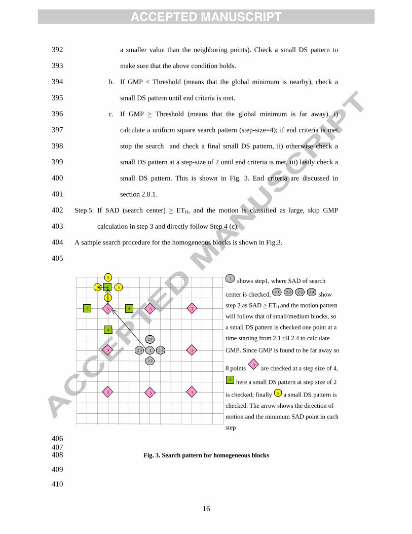
324

2.6. Multiple Initial Predictors 325

Motion vector prediction is used to find the rough initial search center that may lead to the 326

fine search position closer to the global minimum. Our selection of the initial search point is 327

based on the coefficient of homogeneity obtained by homogeneity analysis. For homogenous 328

and stationary blocks, we can safely use the neighboring blocks in the current frame to 329

calculate the predicted motion vector. However for non-homogeneous blocks, we also include 330

the temporal MV for prediction. In this case, we will start our search from multiple starting 331

points to avoid the chance of being trapped in local minimum [19]. 332

333

For stationary and homogenous blocks, predicted motion vector is calculated using PMV1 334

defined by Eq. 2. For non-homogeneous blocks, we search three motion vector predictors i.e. 335

ZMV, PMV1 and PMV2 as defined by Eqs. 1 - 3. 336

337

2.7. Early Termination 338

The early termination (ET) threshold is a very effective way to optimize an algorithm. 339

Fixed ET thresholds are less capable of matching the dynamics and complexity of video 340

14

sequences. Therefore, we have defined an adaptive ET threshold separately for homogenous 341

and non-homogeneous motion blocks. For non-homogeneous blocks a strict threshold has 342

been defined to avoid wrong search. We have chosen the following for our proposed 343

algorithm. 344

For stationary and homogenous blocks, 345

ETH = mean(SADl, SADu) (19) 346

Where ETH is the early termination criterion for homogenous blocks. SADl and SADu are 347

the SAD of left and upper block respectively. 348

For non-homogeneous blocks 349

ETNH = min (SADl, SADu) (20) 350

Where ETNH is the early termination criterion for non-homogenous blocks. 351

352

2.8. Search Patterns 353

Search patterns play an important role in defining the computational complexity of an 354

algorithm. Since searching at an algorithm’s first step is inevitable, therefore the complexity 355

of an algorithm is directly related to the number of search points in the first step. 356

Real video sequences contain a wide range of motion content, distributed along spatial 357

regions whose shape and position change over time. Adaptation to video contents by utilizing 358

multiple patterns has proven to be very successful for fast motion estimation. However, multi 359

pattern solutions are only reliable if it is possible to find a robust pattern selection algorithm. 360

In the proposed algorithm we have used motion classification based on motion homogeneity 361

and global minimum prediction to switch between different search patterns. The choices of 362

dynamic search patterns help avoid large number of initial search points as well as being 363

trapped in local minimum. Different types of search patterns used in proposed algorithm are 364

diamond, square, center biased and uniform. 365

The search pattern and procedure adopted for different types of motion are explained in the 366

following sub-sections: 367

368

15

2.8.1. Stationary Blocks 369

Step 1: If SAD (search center)< ETH stop the search. 370

Step 2: Otherwise search a small DS pattern as shown in Fig. 2. Continue the search till any 371

of the end criteria is met. 372

End Criteria: i) SAD of the minimum location is less than ETH, ii) The minimum location lies 373

at the search center, or, iii) its the end of search window. 374

375

Fig. 2. Search pattern for stationary blocks 376 377

2.8.2 Homogeneous Blocks 378

A block is said to be homogeneous if it follows the following criterion: 379

Homogeneous coefficient < Threshold 380

Step 1: Check SAD of search center. 381

Step 2: If SAD (search center) < ETH , search a small DS pattern and then stop the search. 382

Step 3: If SAD (search center) > ETH, then if the motion is classified as small/medium (based 383

on the magnitude of predicted motion vector PMV1), goto Step 4, else goto Step 5. 384

Step 4: Check the neighboring points for calculating GMP (Global minimum predictor), 385

starting from right horizontal point in clockwise direction, one point at a time, and 386

follow a small DS pattern if the points are not available. Fig. 3 shows an example of 387

points used for calculating GMP, in the 2nd step labeled as 2.1. to 2.4 . However once 388

GMP is calculated say by the help of point 2.2 (if 2.1 is not available), then point 2.3 389

will not be checked. 390

a. If GMP > 1 then stop the search (as it means that the search center may have 391

1

2

2

2

2

2.1

2.1

2.1

1 shows points searched in step 1. 2

shows a small DS pattern searched in step

2, 2.1 shows that the step 2 is continued till

end criteria is met. The arrow points in the

direction of search location that has

minimum value of SAD.

16

a smaller value than the neighboring points). Check a small DS pattern to 392

make sure that the above condition holds. 393

b. If GMP < Threshold (means that the global minimum is nearby), check a 394

small DS pattern until end criteria is met. 395

c. If GMP > Threshold (means that the global minimum is far away), i) 396

calculate a uniform square search pattern (step-size=4); if end criteria is met 397

stop the search and check a final small DS pattern, ii) otherwise check a 398

small DS pattern at a step-size of 2 until end criteria is met, iii) lastly check a 399

small DS pattern. This is shown in Fig. 3. End criteria are discussed in 400

section 2.8.1. 401

Step 5: If SAD (search center) > ETH, and the motion is classified as large, skip GMP 402

calculation in step 3 and directly follow Step 4 (c). 403

A sample search procedure for the homogeneous blocks is shown in Fig.3. 404

405

406 407

Fig. 3. Search pattern for homogeneous blocks 408

409

410

1 shows step1, where SAD of search

center is checked, 2.1. 2.2 2.3 2.4 show step 2 as SAD > ETH and the motion pattern

will follow that of small/medium blocks, so

a small DS pattern is checked one point at a

time starting from 2.1 till 2.4 to calculate

GMP. Since GMP is found to be far away so

8 points 3

are checked at a step size of 4, 4 here a small DS pattern at step size of 2

is checked; finally 5 a small DS pattern is

checked. The arrow shows the direction of

motion and the minimum SAD point in each

step

1 2.1.

2.2

2.3 2.4

3

3.

3

3 3

3

3 3

4

4

4

4

5

5 5

5

17

2.8.3 Non-Homogeneous Blocks 411

For non-homogeneous blocks, the motion can be considered high, irregular and unpredictable. 412

Here we start our search from multiple starting points [19] using spatial predictor PMV1, 413

temporal predictor PMV2 and ZMV so as to be sure to get true motion without being trapped 414

in local minimum. The search procedure is described as follows: 415

416

Step 1: Check multiple starting points, and stop the search if SAD (search center) < ETNH. 417

Step 2: Otherwise check a large square search pattern that consists of 12 points as shown in 418

Fig 4. This very large pattern is selected to incorporate any irregularity that could 419

exist because of the non-homogeneous nature of the neighboring blocks. 420

Step 3: Check a small DS pattern at a step size of 2 till end criteria is met. 421

Step 4: Finally check a small DS pattern. 422

A sample search procedure for the non homogeneous blocks is shown in Fig.4. 423

424

425

Fig. 4. Search pattern for non-homogeneous blocks 426

427

3. Simulation 428

The proposed algorithm is implemented in JM-12.2 [29] of H.264/AVC reference software. 429

In simulation we compare FS, DS, UMHexagonS and the proposed algorithm in terms of 430

1.1

1.2

1.3

2

2

2

22

2

22 2

2 2

2 3

3

3

3

4

4 4

4

In the first step, check multiple starting points 1.1 1.2 1.3 , and choose the one with minimum SAD as

the search center, 1.1 in the case above. A large

square pattern 2 is checked in step 2, in step 3 a

3 small DS pattern at step size 2 is checked and

finally 4 a small DS pattern with step size 1 is

checked. The arrow shows the direction of motion

and the minimum SAD point in each step

18

computations (search speed measured by total encoding time and ME time) and performance 431

(PSNR and bit rate). The simulation is carried out at 4 different quantization parameters 432

(QP=28, 32, 36, 40) in order to test the algorithm at different bit rates. 433

434

For encoding purposes JM-12.2 Main Encoder Profile has been used. For each test 435

sequence only the first frame has been coded as I frame and the remaining frames are coded 436

as P frames. Only one reference frame has been used. Each pixel in the image sequences is 437

uniformly quantized to 8 bits. Sum of absolute difference (SAD) distortion function is used as 438

the block distortion measure (BDM). The search range is set to 16. Image formats used are 439

QCIF and CIF, and sequences are tested at 30 fps (frames per second). The simulation 440

platform in our experiments is a PC with Intel Pentium IV 2.66 GHZ CPU. 441

442

The test sequences used for our experiments are Mobile, Akiyo, Silent and Container. 443

These sequences exhibit a variety of motion that is generally encountered in real video. 444

Homogeneity threshold is set to 6 and GMP is set to 0.75 (experimentally chosen values). 445

Tables 1-6 show the performance comparison of the proposed algorithm with other block 446

matching algorithms. Two different measures are used to calculate the computational 447

efficiency of our algorithm i.e. total time saving and ME time saving. The two performance 448

quality measures are PSNR Gain and increase in Bit Rate. These are computed as follows: 449

450

Total Time Saving = ((Total Time FS- Total Time algorithm) / Total Time FS).100 (21) 451

ME Time Saving = ((ME Time FS- ME Time algorithm) / ME Time FS).100 (22) 452

PSNR Gain = PSNR algorithm - PSNR FS (23) 453

Bit Rate Incr. = ((Bit Rate algorithm - Bit Rate FS) / Bit Rate FS).100 (24) 454

455

Negative value of PSNR gain means decreasing PSNR and positive value means increasing 456

PSNR. Similarly negative bit rate increase means that the bit rate has actually decreased. 457

19

Tables 1-4 show that the proposed algorithm has greater adaptability for the sequences of 458

different kinds. All test sequences achieve high speedup with little degradation in PSNR and 459

negligible increase for bit rate. The test results are shown at different QPs to compare the 460

performance under different bit rates. Table 5 provides the overall average performance 461

comparison for fast search algorithms. The proposed algorithm has achieved an overall 462

average encoder speedup of 72.35% and ME speedup of 82.45%. Its bit rate is increased by 463

only 0.49% while it has a minimal loss in the encoding quality of 0.027 dB. DS has an overall 464

speedup of 66.88% and ME speedup of 75.95%. Its bit rate is increased by 2.01% while loss 465

in the encoding quality is 0.035 dB. UMHexS has an overall speedup of 67.15% and ME 466

speedup of 76.88%. Its bit rate is increased by 0.18% while loss in the encoding quality is 467

0.003 dB. FME [27] that is a recently proposed fast ME algorithm has an overall speedup of 468

62.50% and ME speedup of 80.19%. Its bit rate is increased by 1.25% while loss in the 469

encoding quality is 0.003 dB. 470

471

Table 6 also shows the performance comparison of the proposed algorithm with Full Search 472

algorithm. A variety of test sequences have been used. It has been observed that the proposed 473

algorithm performs very well in terms of quality (PSNR loss ~ 0.04 dB, bit rate increase ~ 474

0.32 %) and speeds up the process by saving more than 70 % computational time. 475

476

Fig. 5 shows the rate distortion comparison of proposed and other fast block matching 477

algorithms at 30 fps. It is clear that the performance of the proposed algorithm is very close to 478

that of the FS algorithm hence showing very good results. 479

20

480

Table 1 Simulation Results for Mobile, QCIF, 30 fps, and 300 frames 481

482

Time (s) Time Saving % QP BMA PSNR

(dB) Bitrate

(Kbits/s) Total ME Total ME

PSNR Loss (dB)

Bit rateIncr.

%

FS 32.98 422.1 94.2 85.9 - - - -

DS 32.94 441.0 17.0 9.5 82.0 89.0 0.04 4.5

UMHexS 32.98 420.1 22.2 14.9 76.4 82.7 - -0.5 28

Proposed 32.96 423.0 15.8 8.6 83.2 90.0 0.02 0.2

FS 29.37 210.4 87.9 80.5 - - - -

DS 29.35 210.4 17.8 10.1 79.7 87.5 0.02 -

UMHexS 29.37 209.8 22.7 14.9 74.2 81.5 - -0.3 32

Proposed 29.34 212.1 15.6 8.2 82.3 89.8 0.03 0.8

FS 26.30 102.6 82.7 75.8 - - - -

DS 26.25 102.7 17.4 10.3 79.0 86.4 0.05 0.1

UMHexS 26.29 102.7 23.1 16.5 72.0 78.2 0.01 0.1 36

Proposed 26.24 104.1 16.1 8.9 80.5 88.3 0.06 1.5

FS 23.69 55.6 78.1 70.7 - - - -

DS 23.64 55.5 18.9 11.8 75.8 83.3 0.05 -0.2

UMHexS 23.67 55.3 23.4 16.5 70.0 76.7 0.02 -0.5 40

Proposed 23.65 56.5 15.6 8.9 80.0 87.4 0.04 1.6

483

21

484 Table 2 Simulation Results for Akiyo, QCIF, 30 fps, and 300 frames 485

486

Time (s) Time Saving % QP BMA PSNR

(dB) Bitrate

(Kbits/s) Total ME Total ME

PSNR Loss (dB)

Bit rateIncr.

%

FS 38.19 25.6 48.9 42.3 - - - -

DS 38.11 25.9 17.4 11.7 64.4 72.3 0.08 1.2

UMHexS 38.19 25.3 16.9 9.9 65.4 76.6 - -1.2 28

Proposed 38.14 25.5 14.1 7.8 71.1 81.6 0.05 -0.4

FS 35.23 14.5 46.7 40.3 - - - -

DS 35.20 14.5 18.4 11.9 60.6 70.5 0.03 -

UMHexS 35.27 14.5 16.8 9.9 64.0 75.4 -0.04 - 32

Proposed 35.21 14.6 14.1 7.9 69.8 80.4 0.02 0.7

FS 32.62 8.9 44.1 37.8 - - - -

DS 32.52 8.9 18.7 11.9 57.6 68.5 0.10 -

UMHexS 32.61 8.9 16.9 10.5 61.7 72.2 0.01 - 36

Proposed 32.60 9.1 14.0 7.6 68.3 79.9 0.02 2.2

FS 30.27 6.2 40.8 34.6 - - - -

DS 30.25 7.1 19.9 13.7 51.2 60.4 0.02 14.5

UMHexS 30.29 6.2 17.3 11.0 57.6 68.1 -0.02 - 40

Proposed 30.30 6.3 13.8 7.7 66.2 77.7 -0.03 1.6

487

22

488 Table 3 Simulation Results for Silent, QCIF, 30 fps, and 100 frames 489

490

Time (s) Time Saving % QP BMA PSNR

(dB) Bitrate

(Kbits/s) Total ME Total ME

PSNR Loss (dB)

Bit rateIncr.

%

FS 35.67 82.95 20.8 18.3 - - - -

DS 35.61 85.57 5.8 3.4 72.1 83.0 0.06 3.2

UMHexS 35.67 83.21 6.1 3.4 70.7 83.0 - 0.3 28

Proposed 35.62 85.72 5.3 2.9 74.5 84.2 0.05 3.3

FS 32.78 48.89 19.6 17.3 - - - -

DS 32.73 49.35 6.2 3.9 68.4 77.5 0.05 0.94

UMHexS 32.77 48.9 6.3 3.8 67.9 78.0 0.01 - 32

Proposed 32.73 50.4 5.2 2.8 73.5 83.8 0.05 3.1

FS 30.28 28.7 18.7 16.3 - - - -

DS 30.24 28.9 6.2 3.7 66.8 77.3 0.04 0.9

UMHexS 30.25 28.7 6.3 3.9 66.3 76.1 0.03 - 36

Proposed 30.23 29.2 5.2 3.3 72.1 79.8 0.05 1.7

FS 27.91 16.9 17.7 15.83 - - - -

DS 27.88 17.1 6.6 4.5 62.7 71.6 0.03 0.9

UMHexS 27.89 16.6 6.5 4.3 63.3 72.8 0.02 -2.1 40

Proposed 27.91 17.1 5.1 3.1 71.2 80.4 - 0.9

491

23

492 Table 4 Simulation Results for Container, QCIF, 30 fps, and 100 frames 493

494

Time (s) Time Saving % QP BMA PSNR

(dB) Bitrate

(Kbits/s) Total ME Total ME

PSNR Loss (dB)

Bit rateIncr.

%

FS 36.06 41.4 19.2 16.8 - - - -

DS 36.04 43.4 5.8 3.3 69.8 80.4 0.02 4.83

UMHexS 36.04 41.3 5.2 2.8 72.9 83.2 0.02 -0.2 28

Proposed 36.04 41.5 4.9 2.9 74.5 82.7 0.02 0.2

FS 33.37 22.2 16.8 14.8 - - - -

DS 33.36 22.4 5.9 3.9 64.9 73.6 0.01 0.9

UMHexS 33.37 22.1 5.3 3.3 68.5 77.8 - 0.5 32

Proposed 33.34 22.1 4.9 2.7 70.8 81.8 0.03 0.5

FS 30.74 12.9 15.2 12.9 - - - -

DS 30.76 13.0 6.1 4.1 59.9 68.2 -0.02 0.8

UMHexS 30.74 12.9 5.4 3.0 64.5 76.4 - - 36

Proposed 30.74 12.8 4.9 2.7 67.8 79.1 - -0.8

FS 28.35 8.4 13.7 11.5 - - - -

DS 28.34 8.5 6.2 4.0 54.8 65.2 0.01 1.1

UMHexS 28.34 8.5 5.4 3.2 60.6 71.7 0.01 1.1 40

Proposed 28.29 8.4 4.8 2.5 65.0 78.3 0.06 -

495

24

496 Table 5 Average performance comparison with respect to FS 497

Time Saving % Algorithm

Total ME PSNR

Loss(dB) Bit rate

Increase (%)

Mobile Sequence QCIF, 300 frames

DS 79.1 86.6 0.04 1.0

UMHexS 73.2 79.8 0.01 -0.3

FME 52.56 81.30 0.01 3.0

Proposed 81.5 88.9 0.04 1.0

Akiyo Sequence QCIF, 300 frames

DS 58.5 67.9 0.06 3.9

UMHexS 62.2 73.1 -0.01 0.3

FME 66.24 79.70 0.02 0.05

Proposed 68.9 79.9 0.02 1.0

Silent Sequence QCIF, 100 frames

DS 67.5 77.4 0.05 1.5

UMHexS 66.9 77.5 0.02 -0.5

FME 64.36 81.07 -.01 2.2

Proposed 72.8 82.1 0.04 2.3

Container Sequence QCIF, 100 frames

DS 62.4 71.9 0.01 1.63

UMHexS 66.6 77.3 0.01 0.35

FME 66.84 78.72 -.01 -.26

Proposed 69.5 80.5 0.03 -0.03

Average

DS 66.88 75.95 0.035 2.01

UMHexS 67.15 76.88 0.003 0.18

FME 62.50 80.19 0.003 1.25

Proposed 72.35 82.45 0.027 0.49 498

25

499

Mobile QCIF 30 Hz

28

29

30

31

175 200 225 250 275Bit Rate (kbps)

PSN

R (d

B)

FSDSUMHexSProposed

500

(a) 501

502

Akiyo QCIF 30 Hz

35

36

37

38

16 18 20 22 24Bit Rate (kbps)

PSN

R (d

B)

FSDSUMHexSProposed

503

(b) 504

505

506

507

508

509

26

Silent QCIF 30 Hz

27

28

29

30

31

18 20 22 24 26Bit Rate (kbps)

PSN

R (d

B)

FSDSUMHexSProposed

510

(c) 511

512

Container QCIF 30 Hz

33

34

35

36

25 31 37 43Bit Rate (kbps)

PSN

R (d

B)

FSDSUMHexSProposed

513 514

(d) 515

Fig. 5 Comparison of Rate-Distortion curves for different block matching algorithms, a closer 516

view, (a) Mobile, (b) Akiyo, (c) Silent, (d) Container 517

518

519

520

521

27

Table 6 Performance comparison with respect to FS 522

QP=28, 30 fps, and 100 frames 523

524

Time (s) Time Saving %Sequence BMA PSNR

(dB) Bit rate

(Kbits/s) Total ME Total ME

PSNR Loss (dB)

Bit rateIncr.

%

FS 37.22 60.65 15.99 13.74 - - - - Hall Monitor QCIF Proposed 37.19 61.51 4.99 2.55 68.8 81.4 0.03 1.41

FS 39.84 33.40 13.96 11.61 - - - - Claire QCIF Proposed 39.77 33.14 4.81 2.71 65.5 76.66 0.07 -0.78

FS 36.70 76.68 17.64 15.44 - - - - News QCIF Proposed 36.68 77.67 5.05 2.71 71.37 82.45 0.02 1.29

FS 33.95 1922.47 125.59 114.99 - - - - Mobile CIF Proposed 33.92 1909.23 23.50 12.94 81.30 88.75 0.03 -0.69

FS 35.84 199.71 89.89 81.1 - - - - Container CIF Proposed 35.82 200.46 20.93 12.02 76.72 85.18 0.02 0.38

Average 72.74 82.89 0.04 0.32

525 526

4. Conclusion 527

In this paper, we propose a fast motion estimation algorithm using the local motion 528

statistics of neighboring motion vectors in spatial and temporal domain. The motion 529

characteristics of the video sequences are studied using homogeneity analysis, based on which 530

the motion is classified into uniform or random. This helps to choose between different search 531

patterns that matches the wide range of motion content. The early termination criteria are also 532

dynamically chosen for different cases. The novelty of this paper is that by using a multistage 533

approach, the proposed algorithm has reduced the computational cost significantly without 534

sacrificing the visual quality and coding performance. 535

536

537

28

References 538

[1] D. LeGall, “MPEG: A video compression standard for multimedia,” Commun. ACM, Vol. 34, No. 539

4, pp. 47-58, Apr. 1991. 540

[2] ISO/IEC JTC// SC29/WG11 moving picture experts group, MPEG2 test model 4, 1993. 541

[3] CCITT SG XV, “Recommendation H.261 video codec for audiovisual services at p*64 kbits/sec” 542

Tech. Rep. COMXVR37-E, Aug. 1990. 543

[4] T. Wiegand, G. Sullivan, A. Luthra, “Draft ITU-T Recommendation and Final Draft International 544

Standard of Joint Video Specification (ITU-T Rec. H.264| ISO/IEC 14496-10 AVC)”, May 2003. 545

[5] T. Koga, K. Iinuma, A. Hirano, Y. Iijima and T. Ishiguro, "Motion compensated interframe coding 546

for video conferencing," Pro. Nat. Telecommun. Conf., New Orleans, pp. G5.3.1-5.3.5, Nov. 1981. 547

[6] R. Li, B. Zeng and M. L. Liou, "A new three step search algorithm for block motion estimation,” 548

IEEE Trans. Circuits Syst. Video Technol., Vol. 4, No. 4, pp. 438-442, Aug. 1994. 549

[7] L. M. Po and W. C. Ma, “A novel four-step search algorithm for fast block motion estimation,” 550

IEEE Trans. Circuits Syst. Video Technol., Vol. 6, No. 3, pp. 313-317, Jun. 1996. 551

[8] S. Zhu and K. K. Ma, “A new diamond search algorithm for fast block matching motion 552

estimation,” IEEE Trans. Image Process., Vol. 9, No. 2, pp. 287-290, Feb 2000. 553

[9] Ce Zhu, Xiao Lin, and Lap-Pui Chau, Hexagon-based search pattern for fast block motion 554

estimation, ,” IEEE Trans. Circuits Syst. Video Technol., Vol. 12, No. 5, pp. 349-355, May 2002. 555

[10] Z. Chen, P. Zhou, Y. He and Y. Chen, “Fast Integer Pel and Fractional Pel Motion Estimation for 556

JVT” ITU-T, Doc. #JVT-F-017, Dec. 2002.” 557

[11] Y. Nie and K.-K. Ma, "Adaptive rood pattern search for fast block-matching motion estimation," 558

IEEE Trans. on Image Processing, Vol. 11, No. 12, pp. 1442-1449, Dec. 2002. 559

[12] Ma, K-K and G Qui, "An improved adaptive rood pattern search for fast block-matching motion 560

estimation in JVT/H.26L," Proceedings of the IEEE Int. Symposium on Circuits and Systems, vol. 561

2, pp. 708-711, May 2003. 562

[13] Byung-Gyu Kim, Suk-Kyu Song and Pyoung-Soo Mah, “Enhanced block motion estimation based 563

on distortion-directional search patterns,” Pattern Recognition Letters, Volume 27, Issue 12, pp. 564

1325-1335 September 2006. 565

[14] Ahmad, W. Zheng, J. Luo, and M. Liou, “A fast adaptive motion estimation algorithm,” IEEE 566

Trans. Circuits Syst. Video Technol. Vol. 16 No. 3 pp. 420–438, 2006. 567

29

[15] 19. S.-C. Tai, C.-S. Yu, and F.-K. Huang, “Fast motion estimation algorithm using motion 568

adaptive search,” Opt. Eng. Vol. 47, No. 3, 037007, 2008. 569

[16] Humaira Nisar, Tae-Sun Choi, “A fast block motion estimation algorithm based on motion 570

classification and directional search patterns”, Optical Engineering, Vol. 47, No. 10, pp. 107001.1-571

10, Oct. 2008. 572

[17] H. Nisar, T.-S. Choi, “Fast motion estimation algorithm based on spatio-temporal correlation and 573

direction of motion vectors,” Electron. Lett. 42 (24) (2006) 1384–1385. 574

[18] Humaira Nisar, Tae Sun Choi, “A Content Aware Fast Motion Estimation Algorithm for 575

H.264/AVC”, Invited Paper, International Symposium on Signal Processing, Image Processing and 576

Pattern Recognition, SIP 2008, China, Dec. 2008. 577

[19] Humaira Nisar, Tae-Sun Choi, “Multiple Initial Point Prediction based Search Pattern Selection for 578

Fast Motion Estimation”, Pattern Recognition, Vol. 42, No. 3, pp. 475-486, Mar. 2009. 579

[20] Jiancong Luo, Ishfaq Ahmad, Yongfang Liang and Viswanathan Swaminathan, "Motion 580

estimation for content adaptive video compression", IEEE Trans. Circuits Syst. Video Technol., 581

Vol. 18, No. 17, pp. 900-909, Jul. 2008. 582

[21] Jun Zhang, Xiaoquan Yi, Nam Ling and Weijia Shang, "Context adaptive Lagrange multiplier 583

(CALM) for rate-distortion optimal motion estimation in video coding", IEEE Trans. Circuits Syst. 584

Video Technol., Vol. 20, No. 6, Jun 2010. 585

[22] C, Zhu, X. Lin, L. P. Chau and L. M. Po, “Enhanced hexagonal search for fast block motion 586

estimation,” IEEE Trans. Circuits Syst. Video Technol., Vol. 14 No. 10, pp. 1210-1214, Oct. 2004. 587

[23] J.J. Tsai and H. M. Hang, “Modeling of pattern based block motion estimation and its application,” 588

IEEE Trans. Circuits Syst. Video Technol., Vol. 19, No. 1, pp. 1210-1214, Jan. 2009. 589

[24] Ka-Ho Ng, Lai. Man Po and Ka-Man Wong, “Search patterns switching for motion estimation 590

using rate of error descent,” pp. 1583-1586, ICME 2007. 591

[25] Liu, L.-K., and Feig, E, “A block-based gradient descent search algorithm for fast block motion 592

estimation in video coding,” IEEE Transactions on Circuits and Systems for Video Technology, 593

Vol. 6 No. 4, pp. 419–423, 1996. 594

[26] Lili Hsieh, Wen-Shiung Chen, Chuan-Hsi Liu, “Motion estimation using two-stage predictive 595

search algorithms based on joint spatio-temporal correlation information,” Expert Systems with 596

Applications, 38, 11608–11623, 2011. 597

30

[27] Canhui Cai, Huanqiang Zeng, Sanjit K. Mitra, “Fast Motion Estimation for H.264,” Signal 598

Processing: Image Communication, Vol. 24, pp. 630-636, 2009. 599

[28] Yi Ching Liaw, Jim Z. C. Lai and Zuu Chang Hong, “Fast block matching using prediction and 600

rejection criteria,” Signal Processing, Vol. 89, pp. 1115-1120, 2009. 601

[29] Joint Video Team Reference Software, Version 12.2 (JM12.2), 602

http://iphome.hhi.de/suehring/tml/download/. 603

31

[30] 604

605

Content adaptive fast motion estimation based on spatio-temporal 606

homogeneity analysis and motion classification 607

608

609

1. Local motion statistics decrease effect of unimodal error surface assumption. 610

2. Homogeneity analysis classifies motion as uniform or random. 611

3. Dynamic search pattern switching takes into account various motion contents. 612

4. Extensive simulation results affirm the effectiveness of the proposed algorithm. 613

[31] 614