Guidelines for Weighting Factors Adjustment inFinite State Model Predictive Control of Power

Converters and DrivesPatricio Cortés, Samir Kouro, Bruno La Rocca,

René Vargas and José RodríguezElectronics Engineering Department

Universidad Técnica Federico Santa MaríaValparaiso, Chile

Email: samir.kouro@ieee.org

José I. León, Sergio Vazquezand Leopoldo G. Franquelo

Electronics Engineering DepartmentUniversity of Seville

Seville, SpainEmail:jileon@zipi.us.es

Abstract—Finite State Model Predictive Control (FS-MPC) hasemerged as a promising control tool for power converters anddrives. One of the major advantages is the possibility to controlseveral system variables with a single control law, by includingthem with appropriate weighting factors. However, at the presentstate of the art, these coefficients are determined empirically.There is no analytical or numerical method proposed yet to obtainan optimal solution. In addition, the empirical method is notalways straightforward, and no procedures have been reported.This paper presents a first approach to a set of guidelinesthat reduce the uncertainty of this process. First a classificationof different types of cost functions and weighting factors ispresented. Then the different steps of the empirical process areexplained. Finally, results for several power converters and drivesapplications are presented, which show the effectiveness of theproposed guidelines to reach appropriate weighting factors.

I. INTRODUCTION.

The continuous evolution and growing capabilities of mod-ern microprocessors and signal processing technologies, hasenabled the implementation of more sophisticated controlmethods devised to fulfill the industry’s increasing demand forhigher performance. Predictive control is one of these methods,and has gained recently more attention specially for powerconverter and drive applications [1]. In essence predictivecontrol is a group of different control methods that shareone common characteristic, which is, the use of mathematicalmodels of the system to predict future behaviors and selectappropriate control actions. Several predictive control methodshave been applied to power converter and drive systems,among them: Dead Beat Control [2]–[8], Model PredictiveControl (MPC) [9], [10], Generalized Predictive Control [11],and Finite State Model Predictive Control (FS-MPC) [12].

FS-MPC can be described as a particular case of MPCwhich takes into account the inherent discrete nature of thepower converter switching states and the digital implementa-tion. Since power converters have a finite number of switchingstates, the MPC optimization problem can be simplified andreduced to the prediction of the system behavior only forthose possible switching states. The finite number of system

predictions are used to evaluate a cost function (also knownas quality or decision function), which usually is composedby the errors of the controlled variables. Hence, the switchingstate associated with the prediction that minimizes the costfunction is selected and generated by the converter. Withthis approach the number of calculations is greatly reduced,making realtime implementations feasible with current micro-processor technology. FS-MPC has been successfully appliedto a wide range of power converters and drives applications[12]–[28].

One of the major advantages of FS-MPC is that severalcontrol targets, variables and constraints can be included ina single cost function and simultaneously be controlled. Inthis way traditional variables such as current, voltage, torqueor flux can be controlled while achieving additional controlrequirements like switching frequency reduction, commonmode voltage reduction and reactive power control, to namea few. This can be accomplished simply by introducing theadditional control targets in the cost function to be evaluatedfor the different switching states. However, the combination ofvariables that most likely are of different nature (different unitsand different orders of magnitude) in a single cost functionis not a straightforward task. Each additional term in the costfunction has a corresponding weighting factor, which is used totune the importance or cost of that term in relation to the otherscontrol targets. These parameters have to be properly designedin order to achieve the desired performance. Unfortunately,there are no analytical or numerical methods or control designtheories to adjust these parameters, and currently they aredetermined based on empirical procedures. Although this chal-lenge has not kept back FS-MPC to be applied successfully toseveral power converters, it is highly desirable to establisha procedure or define some basic guidelines to reduce theuncertainty and improve the effectiveness of the tuning stage.

This paper presents a first approach to address thischallenge. First some representative examples of FS-MPCcost functions are classified according to the nature of theirterms, in order to group types of weighting factors that

could be tuned similarly. Then a set of simple guidelinesare analyzed and tested to evaluate the evolution of thesystem performance in relation to changes in the weightingfactors. Several converter and drive control applications willbe studied to cover a wide variety of cost functions andweighting factors. In addition, results for three differentweighting factors are presented to compare results andvalidate the methodology.

II. FINITE STATE MODEL PREDICTIVE CONTROLOVERVIEW.

Consider the generic and simplified block diagram of FS-MPC illustrated in Fig. 1, that controls a system variable xthrough a control action S, usually the gating signals of aconverter. The measured variable x(tk) is fed back and used toevaluate a discrete predictive model or function of the systemfp, to obtain the predicted future values of the system xp

i (tk+1)for each possible control action Si

xpi (tk+1) = fp{x(tk), Si} ∀i = 1, . . . , n. (1)

Note that n corresponds to a finite number of control actionsor switching states. Then the n predictions together with thereference are evaluated in a cost function fg, leading to ndifferent costs g

gi = fg{x∗, xpi } ∀i = 1, . . . , n. (2)

Since the target is to control variable x, usually the costfunction fg is defined by a measure of the error with respectto the reference. Some example of generic cost functions arethe absolute error, quadratic error and mean value of the error

gi = |x∗ − xpi (Si)|,

gi = [x∗ − xpi (Si)]

2, (3)

gi =1Ts

∫ TS

[x∗(t)− xpi (t, Si)]dt.

Note that the next control action S(tk+1) will be theswitching state that minimizes the cost function fg

S(tk+1) = minSi

fg{x∗, xpi (Si)} ∀i = 1, . . . , n. (4)

It is clear that FS-MPC takes advantage of the discretenature of power converters by relating the switching state

Fig. 1. FS-MPC generic simplified control diagram.

directly to the control error. In addition, since the switchingstate is directly chosen from the cost function minimization,no linear controllers and modulators are necessary. This con-trol principle has been successfully applied to several powerconverter and drive control systems, including: voltage sourceinverters, multilevel inverters, matrix converters, regenerativerectifiers and torque control of ac motors, to name a few[11]–[28].

III. COST FUNCTION CLASSIFICATION.Although the cost function’s main objective is to keep track

of a particular variable and control the system, it is not limitedto only do so. In fact one of the main advantages of FS-MPCis that the cost function admits any necessary term that couldrepresent a prediction for another system variable, systemconstraint or system requirement. This flexibility enables FS-MPC to achieve easier more control targets that can translate toincreased system performance, efficiency, power quality, safetyand other possible figures of merit. Since these terms mostlikely can be of different physical nature (current, voltage,reactive power, switching losses, torque, flux, etc.) it can leadto coupling effects between variables, or to overestimate theimportance of one term respect the others in the cost function,making their presence not worth, hence not controllable.

As mentioned before this issue has been commonly dealtwith in MPC by including weighting coefficients or weightingfactors λ, for each term of the cost function

g = λx|x∗ − xp|+ λy|y∗ − yp|+ . . . + λz|z∗ − zp|. (5)

Depending on the nature of the different terms involved inthe formulation of the cost function, they can be classifiedin different groups. This classification is necessary in orderto facilitate the definition of a weighting factor adjustmentprocedure that could be applied to similar types of costfunctions or alike terms.

A. Cost functions without weighting factors.In these kind of cost functions, only one, or the components

of one variable, are controlled. This is the simplest case, andsince only one type of variable is controlled, no weightingfactors are necessary. Some representative examples of thistype of cost functions are obtained for: predictive currentcontrol of a voltage source inverter [14], predictive powercontrol of a back to back ac/dc/ac converter [16], predictivevoltage control of an UPS system [24] and predictive currentcontrol with imposed switching frequency [18], among others.The corresponding cost functions are summarized in Table I.

TABLE ICOST FUNCTIONS WITHOUT WEIGHTING FACTORS.

Application Cost function

Current control of a VSI |i∗α − ipα|+ |i∗β − ipβ |Power control of ac/dc/ac converter |Qp|+ |P ∗ − P p|

Voltage control of UPS (v∗cα − vpcα)2 + (v∗cβ − vp

cβ)2

Imposed switching frequency in a VSI |F (i∗α − ipα)|+ |F (i∗β − ipβ)|

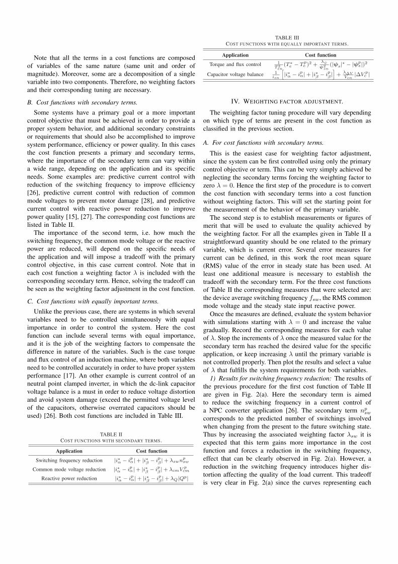
Note that all the terms in a cost functions are composedof variables of the same nature (same unit and order ofmagnitude). Moreover, some are a decomposition of a singlevariable into two components. Therefore, no weighting factorsand their corresponding tuning are necessary.

B. Cost functions with secondary terms.

Some systems have a primary goal or a more importantcontrol objective that must be achieved in order to provide aproper system behavior, and additional secondary constraintsor requirements that should also be accomplished to improvesystem performance, efficiency or power quality. In this casesthe cost function presents a primary and secondary terms,where the importance of the secondary term can vary withina wide range, depending on the application and its specificneeds. Some examples are: predictive current control withreduction of the switching frequency to improve efficiency[26], predictive current control with reduction of commonmode voltages to prevent motor damage [28], and predictivecurrent control with reactive power reduction to improvepower quality [15], [27]. The corresponding cost functions arelisted in Table II.

The importance of the second term, i.e. how much theswitching frequency, the common mode voltage or the reactivepower are reduced, will depend on the specific needs ofthe application and will impose a tradeoff with the primarycontrol objective, in this case current control. Note that ineach cost function a weighting factor λ is included with thecorresponding secondary term. Hence, solving the tradeoff canbe seen as the weighting factor adjustment in the cost function.

C. Cost functions with equally important terms.

Unlike the previous case, there are systems in which severalvariables need to be controlled simultaneously with equalimportance in order to control the system. Here the costfunction can include several terms with equal importance,and it is the job of the weighting factors to compensate thedifference in nature of the variables. Such is the case torqueand flux control of an induction machine, where both variablesneed to be controlled accurately in order to have proper systemperformance [17]. An other example is current control of anneutral point clamped inverter, in which the dc-link capacitorvoltage balance is a must in order to reduce voltage distortionand avoid system damage (exceed the permitted voltage levelof the capacitors, otherwise overrated capacitors should beused) [26]. Both cost functions are included in Table III.

TABLE IICOST FUNCTIONS WITH SECONDARY TERMS.

Application Cost function

Switching frequency reduction |i∗α − ipα|+ |i∗β − ipβ |+ λswnpsw

Common mode voltage reduction |i∗α − ipα|+ |i∗β − ipβ |+ λcmV pcm

Reactive power reduction |i∗α − ipα|+ |i∗β − ipβ |+ λQ|Qp|

TABLE IIICOST FUNCTIONS WITH EQUALLY IMPORTANT TERMS.

Application Cost function

Torque and flux control 1T2

en(T ∗e − T p

e )2 +λψ

ψ2sn

(|ψs|∗ − |ψps |)2

Capacitor voltage balance 1isn

[|i∗α − ipα|+ |i∗β − ipβ |

]+ λ∆V

Vcn|∆V p

c |

IV. WEIGHTING FACTOR ADJUSTMENT.

The weighting factor tuning procedure will vary dependingon which type of terms are present in the cost function asclassified in the previous section.

A. For cost functions with secondary terms.

This is the easiest case for weighting factor adjustment,since the system can be first controlled using only the primarycontrol objective or term. This can be very simply achieved beneglecting the secondary terms forcing the weighting factor tozero λ = 0. Hence the first step of the procedure is to convertthe cost function with secondary terms into a cost functionwithout weighting factors. This will set the starting point forthe measurement of the behavior of the primary variable.

The second step is to establish measurements or figures ofmerit that will be used to evaluate the quality achieved bythe weighting factor. For all the examples given in Table II astraightforward quantity should be one related to the primaryvariable, which is current error. Several error measures forcurrent can be defined, in this work the root mean square(RMS) value of the error in steady state has been used. Atleast one additional measure is necessary to establish thetradeoff with the secondary term. For the three cost functionsof Table II the corresponding measures that were selected are:the device average switching frequency fsw, the RMS commonmode voltage and the steady state input reactive power.

Once the measures are defined, evaluate the system behaviorwith simulations starting with λ = 0 and increase the valuegradually. Record the corresponding measures for each valueof λ. Stop the increments of λ once the measured value for thesecondary term has reached the desired value for the specificapplication, or keep increasing λ until the primary variable isnot controlled properly. Then plot the results and select a valueof λ that fulfills the system requirements for both variables.

1) Results for switching frequency reduction: The results ofthe previous procedure for the first cost function of Table IIare given in Fig. 2(a). Here the secondary term is aimedto reduce the switching frequency in a current control ofa NPC converter application [26]. The secondary term np

sw

corresponds to the predicted number of switchings involvedwhen changing from the present to the future switching state.Thus by increasing the associated weighting factor λsw it isexpected that this term gains more importance in the costfunction and forces a reduction in the switching frequency,effect that can be clearly observed in Fig. 2(a). However, areduction in the switching frequency introduces higher dis-tortion affecting the quality of the load current. This tradeoffis very clear in Fig. 2(a) since the curves representing each

0 0.02 0.04 0.06 0.08 0.10

0.1

0.2

0.3

0.4

0.5

RM

S c

urr

en

t e

rro

r [A

]

Weighting factor λsw

0

200

400

600

800

1000

De

vic

e fs

w [H

z]

(a)

0 0.01 0.02 0.03 0.04 0.06-20

-10

0

10

20

Lo

ad

cu

rre

nt [A

]

0.05

0 0.01 0.02 0.03 0.04 0.05 0.06-400

-200

0

200

400

Time [s]

Lo

ad

vo

lta

ge

[V

] λ =0.1swλ =0sw λ =0.05sw

λ =0.1swλ =0sw λ =0.05sw

Time [s]

(b)

Fig. 2. a) Weighting factor influence over the current error and thedevice average switching frequency fsw . b) Results comparison for differentweighting factors (load current and load voltage).

measure have opposite evolutions for the different valuesof λsw. A suitable selection of λsw would be any value0.04 ≤ λsw ≤ 0.06 since the current error is still below 10%of the nominal current (15[A] in this example) and a reductionfrom 1000[Hz] to 500[Hz] is achieved for the average deviceswitching frequency. Finally λsw = 0.05 has been selected.Figure 2(b) shows comparative results for the system workingwith three different values of λsw, one of them the selectedvalue. Note how the load current presents higher distortionfor the larger value of λsw due to the strong reduction of thenumber of commutations. On the other hand for λsw = 0 thecurrent control works at its best, however at expense of higherswitching losses. Since the NPC is aimed for medium voltagehigh power applications where losses become important, theselection of λsw = 0.05 merges efficiency with performance.

2) Results for common mode voltage reduction: The guide-lines have been used to tune the weighting factor of the secondequation of Table II, which corresponds to predictive currentcontrol of a matrix converter [28]. Here the additional termV p

cm is the predicted common mode voltage for the differentswitching states and it will be considered an additional costby tuning properly the weighting factor λcm. The measures

0 0.1 0.2 0.3 0.4 0.50

0.01

0.02

0.03

0.04

0.05

Weighting factor λcm

RM

S c

urr

en

t e

rro

r [A

]

0

25

50

75

100

125

RM

S c

om

mo

n

mo

de

vo

ltag

e [V

]

(a)

0 0.01 0.02 0.03 0.04-200

-100

0

100

200

Time [s]

CM

vo

lta

ge

[V

]

λ =0.05cmλ =0cm λ =0.15cm λ =0.5cm

0 0.02 0.04 0.06 0.08 0.1-20

-10

0

10

20

Time[s]

Lo

ad

cu

rre

nt [A

]

λ =0.05cmλ =0cm λ =0.15cm λ =0.5cm

(b)

Fig. 3. a) Weighting factor influence over the current error and the commonmode voltage. b) Results comparison for different weighting factors (loadcurrent and common mode voltage).

that will be used to evaluate the different λcm are the RMScurrent error and the RMS common mode voltage. Figure 3(a)shows the results obtained following the proposed procedure.Note that, like for the previous case, similar evolutions of bothmeasures are obtained, i.e, for higher values of λcm smallerCM voltage are obtained, while the current control becomesless important and looses some performance. The result showsalso that CM voltages is a variable more decoupled of the loadcurrent compared to the switching frequency since the currenterror remains very low throughout the wide range of λcm.Hence the selection of a appropriate value is easier, and valuesof λcm ≥ 0.05 will perform well. This can be observed for theresults shown in Fig. 3, where clearly a notorious reductionof the CM voltages is achieved without affecting the currentcontrol.

3) Results for input reactive power reduction: The last costfunction of Table II corresponds to a current control of amatrix converter [27] with input power factor correction. Theadditional term in the cost function is directly the predictedinput reactive power Qp with its corresponding weightingfactor λQ. The measures used to tune λQ are the RMS currenterror and the input reactive power.

0 0.05 0.1 0.15 0.2 0.25 0.30

0.02

0.04

0.06

0.08

Weighting factor λQ

RM

S c

urr

en

t e

rro

r [A

]

0

300

600

900

1.200 Re

activ

e p

ow

er [W

]

(a)

0 0.02 0.04 0.06 0.08-20

-10

0

10

20

Time [s]

Lo

ad

cu

rre

nt [A

]

λ =0.05Qλ =0Q λ =0.3Q

0 0.02 0.04 0.06 0.08-4000

-2000

0

2000

4000

Time [s]

Re

active

po

we

r [W

]

λ =0.05Qλ =0Q λ =0.3Q

(b)

Fig. 4. a) Weighting factor influence over the current error and the inputreactive power. b) Results comparison for different weighting factors (loadcurrent and input reactive power).

The results of the tuning procedure are depicted in Fig. 4(a).Since this cost function belongs to the same classification asthe previous two, it is expected to present similar measure-ments evolution when increasing λQ. As with the previouscase, the input reactive power seems to be very decoupledof the load current, hence the current error remains very lowfor a wide range of λQ. It becomes easy to obtain a suitablevalue considering λQ ≥ 0.05. This can be corroborated withthe results given in Fig. 4(b), showing an important reductionof the input reactive power for λQ = 0.05.

The proposed procedure can be programmed by automatingand repeating the simulation introducing an increment in theweighting factor after each simulation. An other way is toreduce the number of repetitions, by applying a branch andbound algorithm. For this approach first select a couple ofinitial values for λ, usually with different orders of magnitudeto cover a very wide range λ=0, 0.1, 1 and 10, for example.A qualitative example of this algorithm is illustrated in Fig. 5.Then simulate for these weighting factors and obtain themeasures for both terms, M1 and M2 for the primary andsecondary terms respectively. Then compare these results withthe desired maximum errors admitted by the application andfit them into an interval of two weighting factors (0.1 ≤ λ ≤ 1

< λ <

Start

M1(λ0), M2(λ0) M1(λ0.1), M2(λ0.1) M1(λ1), M2(λ1) M1(λ10), M2(λ10)

λ = 0 λ = 0.1 λ = 1 λ = 10

M1(λ0.1), M2(λ0.1) M1(λ1), M2(λ1)M1(λ0.5), M2(λ0.5)

λ = 0.5

M1(λ0.25), M2(λ0.25)

λ = 0.25

M1(λ0.1), M2(λ0.1) M1(λ0.5), M2(λ0.5)

0.1 0.25

Fig. 5. Branch and bound algorithm to reduce simulations to obtain suitableweighting factors.

in the example). Then compute the measures for the λ inthe half of the new interval (λ = 0.5 in the example) andcontinue so on until you achieve a suitable lambda. Note inFig. 5 that each hard line corresponds to a simulation anddashed lines corresponds to values already simulated. Thismethod reduces the number of simulations necessary to obtaina working weighting factor.

The qualitative example of Fig. 5 can be matched with theresults for the common mode reduction case of Fig. 3(a). Notethat with only 7 simulations the search for λcm would havenarrowed to an interval 0.1 ≤ λcm ≤ 0.25 where any λcm

would work properly.

B. For cost functions with equally important terms

For cost functions like those listed in Table III, the proce-dure needs some minor adjustments since λ is not allowedto be zero. Another difficulty is the different nature of thevariables. For example, when controlling torque and flux inan adjustable speed drive application with a nominal torqueand flux of 25[Nm] and 1[Wb] respectively, the torque errorcan have different orders of magnitudes making both variablenot equally important in the cost function, affecting the systemperformance. Thus the fist step is to normalize the cost func-tion. Once normalized, all the terms will be equally importantand now λ = 1 can be considered as starting point. Usually asuitable λ is closely located to 1. Note that the cost functionsin Table III have already included this normalization (nominalvalues are denoted by subindex n).

The second step is the same as with the previous procedure,i.e., measurements or figures of merit have to be defined thatwill be used to evaluate the quality achieved by the weightingfactor.

The last step is to perform the branch and bound algorithmof Fig. 5 considering a couple of starting points. Naturallyλ = 1 has to be considered, and λ = 0 has to be avoided.When a small interval of weighting factors has been reached,meaning by small interval, that there are no big differencesin the measures between the upper and lower bounds of theinterval, then the weighting factor has been obtained.

-3 -2.5 -2 -1.5 -1 -0.5 0 0.5 1 1.50

0.2

0.4

0.6

0.8

1

RM

S flu

x e

rro

r [W

b]

Weighting factor log10

(λψ )

0

2

4

6

8

10

RM

S to

rqu

e e

rror [N

m]

(a)

0

10

20

30

To

rqu

e [N

m]

0.8

0.9

1

1.1

Flu

x [W

b]

0 0.01 0.02 0.03 0.04 0.05 0.06

λ =10ψλ =0.85ψλ =0.1ψ

λ =10ψλ =0.85ψλ =0.1ψ

0 1.5 3 0 1.5 3 0 1.5 3

-5

0

5

Lo

ad

cu

rre

nt [A

]

0 0.01 0.02 0.03 0.04 0.05 0.06

λ =10ψλ =0.85ψλ =0.1ψ

Time [s]

Time [s]

Time [s]

(b)Fig. 6. a) Weighting factor influence over the flux and torque errors. b)Results comparison for different weighting factors (torque step response, fluxmagnitude in steady state and load currents).

1) Results for torque and flux control: The predictive torqueand flux control of an induction motor speed drive [17], canbe implemented using the first cost function in Table III. Notethat the terms appear already normalized. The two terms inthe cost function are the torque and flux error. Hence themeasures that will be suitable to select the proper λψ willbe the respective RMS errors. A branch and bound algorithmstarting with λψ=0.01,0.1,1,10 and 100 first gave the interval0.1 ≤ λψ ≤ 1, and then 0.5 ≤ λψ ≤ 1 with very smalldifferences. Finally λψ = 0.85 was chosen. Figure 6(a) showsextensive results considering much more values of λψ (notethat the values are represented in log10() scale), to show thatthe branch and bound method really found a suitable solution.

Results for different λψ , including λψ = 0.85 are given inFig. 6(b) to show the performance achieved by the FS-MPC.

Weighting factor log-16 -14 -12 -10 -8 -6 -4 -2 0 2

0

0.05

0.1

0.15

0.2

RM

S c

urr

en

t e

rro

r [A

]

0

5

10

15

20

RM

S V

olta

ge

u

nb

ala

nce

[V]

10(λ∆c )

(a)

0 0.05 0.1 0.15 0.2 0.25 0.3

0

200

400

600

Time [s]

Ca

p. vo

lta

ge

s [V

]

λ =0∆c

λ =0.001∆c

0 0.01 0.02 0.03 0.04 0.05 0.06-400

-200

0

200

400

Time [s]

Lo

ad

vo

lta

ge

[V

]

λ =100∆c

λ =0∆c λ =0.001∆c λ =100∆c

(b)Fig. 7. a) Weighting factor influence over the current error and the dc-linkcapacitors unbalance. b) Results comparison for different weighting factors(load current and dc-link capacitor voltages dynamic behavior).

Note that λψ = 0.85 presents the best combination of torquestep response and steady state, flux control and load currentwaveforms.

2) Results for voltage balancing: The predictive currentcontrol of a NPC converter [26], can be implemented using thesecond cost function in Table III. The additional term ∆V p

c

corresponds to the predicted voltage unbalance of the dc-linkcapacitors of the converter. If this unbalance is not controlled,the dc-link voltages will drift and introduce considerable out-put voltage distortion, no to mention that the dc-link capacitorscould get damaged by overvoltage, unless they are overrated.Note the terms appear already normalized in the cost function,as indicated in the first step of the procedure. The measuresthat will be used to evaluate the weighting factor λ∆V arethe RMS current error and the peak amplitude of the voltageunbalance.

A branch and bound algorithm starting with λ∆V =10−4,10−2, 1, 102 and 104 first gave the interval 10−4 ≤ λ∆V ≤10−2 after this first evaluation very small differences wereobtained. Finally λ∆V = 10−3 was evaluated leading to thesame measures. Hence this value was chosen. Figure 7(a)shows extensive results considering much more values (notethat the values are represented in log10() scale), to show thatthe branch and bound method really found a suitable solution.

Results for different λψ , including λ∆V = 0.001 are givenin Fig. 7(b) to show the performance achieved by the FS-MPC.Note that for λ∆V = 0, which normally is not allowed sinceits does not control the unbalance producing the maximumdrift of the dc-link capacitors, the load voltage only presents5 different voltage levels, while 9 levels should appear inthe load phase-neutral voltage (since the NPC has 3 levelsin the converter phase-neutral voltage). Only 5 appear sincethe NPC is not generating 3 output levels, due to the voltagedrift of its capacitors it is only generating 2 levels. On theother hand, λ∆V = 100 controls the voltage unbalance veryaccurately, it even makes voltage unbalance so important in thecost function that it disables the generation of those switchingstates that produce unbalance eliminating voltage levels at theoutput and increases the switching frequency as can be seenin the load voltage of Fig. 7(b). On the contrary, the selectedλ∆V = 0.001 presents the 9 load voltage levels, controls theload current and keeps the capacitor voltages balanced.

V. CONCLUSION

In this paper the design of the weighting factors used in costfunctions of Finite State Model Predictive Control has beenanalyzed. A first approach based on an empirical procedure toobtain suitable weighting factors has been presented.

For cost functions with a primary control objective andsecondary terms, the starting point is λ=0, then test incrementsof λ until the desired behavior is obtained (branch and boundcan also be used). For cost functions with equally importantterms, first normalize the cost function and set λ = 1, with thisvalue the system will be controlled, for fine tuning use branchand bound or move slightly λ around 1. At least two differentfigures of merit or system parameters have to be considered,depending on the application, to settle the tradeoff present inthe designing choice of the weighting factors.

This contribution is a first design approach to reduce theuncertainty if the cots function design in FS-MPC of systemswith more than one control objective. The examples studied inthis paper show the potential and flexibility of FS-MPC andhow easy it is to include additional control objectives in onesingle controller compared to classic control schemes.

REFERENCES

[1] R. Kennel and A. Linder, “Predictive control of inverter supplied electricaldrives,” IEEE Power Electronics Specialists Conference (PESC 2000), pp.761–766, Galway, Ireland, 2000.

[2] O. Kukrer, “Discrete-time current control of voltage-fed three-phasePWM inverters,” IEEE Trans. on Industrial Electronics, vol. 11, no. 2,pp. 260–269, March 1996.

[3] H.-T. Moon, H.-S. Kim, and M.-J. Youn, “A discrete-time predictivecurrent control for PMSM,” IEEE Trans. On Power Electronics, vol. 18,no. 1, pp. 464–472, January 2003.

[4] L. Springob and J. Holtz, “High-bandwidth current control for torque-ripple compensation in PM synchronous machines,” IEEE Trans. OnIndustrial Electronics, vol. 45, no. 5, pp. 713–721, October 1998.

[5] G. Bode, P. C. Loh, M. J. Newman, and D. G. Holmes, “An improvedrobust predictive current regulation algorithm,” IEEE Trans. on IndustryApplications, vol. 41, no. 6, pp. 1720–1733, November 2005.

[6] S.-M. Yang and C.-H. Lee, “A deadbeat current controller for fieldoriented induction motor drives,” IEEE Trans. on Power Electronics, vol.17, no. 5, pp. 772–778, September 2002.

[7] H. Abu-Rub, J. Guzinski, Z. Krzeminski, and H. A. Toliyat, “Predic-tive current control of voltage source inverters,” IEEE Transactions onIndustrial Electronics, vol. 51, no. 3, pp. 585–593, June 2004.

[8] P. Mattavelli, “An improved deadbeat control for UPS using disturbanceobservers,” Trans. on Industrial Electronics, vol. 52, no. 1, pp. 206–212,Feb. 2005.

[9] E. F. Camacho and C. Bordons, “Model Predictive Control,” Springer-Verlag, 1999.

[10] A. Linder and R. Kennel, “Model predictive control for electrical drives,”in Proc. of IEEE PESC 05, Recife, Brazil, June 12-16 2005, pp. 1793–1799.

[11] R. Kennel, A. Linder, and M. Linke, “Generalized predictive control(GPC)-ready for use in drive applications?” IEEE 32nd Annual PowerElectronics Specialists Conference, PESC01 , vol. 4, pp. 1839–1844,2001.

[12] P. Cortes, J. Rodriguez, R. Vargas, and U. Ammann, “Cost function-based predictive control for power converters,” in IEEE Industrial Elec-tronics, IECON 2006 - 32nd Annual Conference on, Nov. 2006, pp. 2268–2273.

[13] S. Muller, U. Ammann, and S. Rees, “New modulation strategy for amatrix converter with a very small mains filter,” IEEE 33th Annual PowerElectronics Specialists Conference, PESC03, pp. 1275–1280, Acapulco,Mexico, 2003.

[14] J. Rodríguez, J. Pontt, C. Silva, P. Correa, P. Lezana, P. Cortés, and U.Ammann, “Predictive current control of a voltage source inverter,” IEEETrans. on Industrial Electronics, vol. 54, no. 1, pp. 495–503, February2007.

[15] S. Muller, U. Ammann, and S. Rees, “New time-discrete modulationscheme for matrix converters,” IEEE Trans. on Industrial Electronics,vol. 52, no. 6, pp. 1607–1615, December 2005.

[16] J. Rodriguez, J. Pontt, P. Correa, P. Lezana, and P. Cortes, “Predictivepower control of an AC/DC/AC converter,” IEEE Industry ApplicationsSociety Annual Meeting, IAS’05, vol. 2, pp. 934–939, Oct. 2005.

[17] J. Rodriguez, J. Pontt, C. Silva, P. Cortés, S. Rees, and U. Ammann,“Predictive direct torque control of an induction machine,” in 11thInternational Power Electronics and Motion Control Conference, EPE-PEMC 2004, Riga, Latvia, 2-4 September 2004.

[18] P. Cortes, J. Rodriguez, D. E. Quevedo, and C. Silva, “Predictive currentcontrol strategy with imposed load current spectrum,” IEEE Transactionson Power Electronics, vol. 23, no. 2, pp. 612–618, Mar. 2008.

[19] A. Linder and R. Kennel, “Direct model predictive control - a new directpredictive control strategy for electrical drives,” in Power Electronics andApplications, 2005 European Conference on, Sept. 2005.

[20] G. Perantzakis, F. Xepapas, S. Papathanassiou, and S. N. Manias, “Apredictive current control technique for three-level NPC voltage sourceinverters,” in Power Electronics Specialists Conference, 2005. PESC ’05.IEEE 36th, Sept. 2005, pp. 1241–1246.

[21] G. S. Perantzakis, F. H. Xepapas, and S. N. Manias, “Efficient predictivecurrent control technique for multilevel voltage source inverters,” inPower Electronics and Applications, 2005 European Conference on, Sept.2005.

[22] H. Q. S. Dang, P. Wheeler, and J. Clare, “A control analysis andimplementation of high voltage, high frequency direct power converter,”in IEEE Industrial Electronics, IECON 2006 - 32nd Annual Conferenceon, Nov. 2006, pp. 2096–2102.

[23] M. Catucci, J. Clare, and P. Wheeler, “Predictive control strategy for ZCSsingle stage resonant converter,” in IEEE Industrial Electronics, IECON2006 - 32nd Annual Conference on, Nov. 2006, pp. 2905–2910.

[24] P. Cortes and J. Rodriguez, “Three-phase inverter with output LC filterusing predictive control for UPS applications,” in Power Electronics andApplications, 2007 European Conference on, Sept. 2007, pp. 1–7.

[25] E. I. Silva, B. P. McGrath, D. E. Quevedo, and G. C. Goodwin,“Predictive control of a flying capacitor converter,” in Proceedings ofthe American Control Conference, New York City, USA, July 2007.

[26] R. Vargas, P. Cortes, U. Ammann, J. Rodriguez, and J. Pontt, “Predictivecontrol of a three-phase neutral-point-clamped inverter,” IEEE Transac-tions on Industrial Electronics, vol. 54, no. 5, pp. 2697–2705, Oct. 2007.

[27] R. Vargas, M. Rivera, J. Rodríguez, J. Espinoza, Predictive TorqueControl with Input PF Correction applied to an Induction Machine fed bya Matrix Converter, in Conf. Rec. of IEEE PE Society Annual Meeting,PESC 2008, 15-19 June 2008.

[28] R. Vargas, U. Ammann, J. Rodríguez, J. Pontt, Predictive Strategyto Reduce Common-Mode Voltages on Power Converters, in PowerElectronics Specialists Conference, PESC 2008, 15-19 June 2008.