GROUNDWATER MODELLING OF ÄSPÖ USING THE ...

CHALMERS TEKNISKA HÖGSKOLA

GEOLOGISKA INSTITUTIONENPubl. B 417

EXAMENSARBETE

HAYDER WOKIL

GROUNDWATER MODELLING OF ÄSPÖUSING THE ECLIPSE PROGRAM

GOTEBORG 1995

Chalmers tekniska högskolaGEOLOGISKA INSTITUTIONENS-412 96 GöteborgTel. 031-772 2040

Hayder Wokil

Groundwater Modelling of AspöUsing the Eclipse Program

; Publ.B 41x. /Examensarbete

ISSN 1104-9847 Göteborg 1995

DEDICATION

TO MAY MOTHER, WITH ALL LOVE AND RESPECT.

HAYDER

SUPERVISOR'S PREFACE

The ECLIPSE family of computer programs are the petroleum industry "standard" for thesimulation of oil and gas recovery from natural, subsurface reservoirs. There have been recentadvances in this family of software to enhance its utilization in environmental problems.However, very few examples of its application to hydrogeological problems, especially infractured crystalline rock, are available. This project was designed to test the applicability ofECLIPSE 100 simulator to such a geological environment.

The application of the simulator was made to the main fracture zone (Zone NE-1) in the ÄspöHard Rock Laboratory (HRL). This application is one of the very few applications of thissimulator to groundwater flow in a large fracture zone in crystalline rock, but is one of manyattempts to model groundwater flow in the HRL. The present application is not as complex asthe other computer simulations of the groundwater flow at HRL, but its performance in thislimited test is quite encouraging.

The project was carried out by Hayder Wokil, who meticulously adapted the petroleum-basedsimulation to a water-based simulation. He also modified the "classical" use of the simulatorfor granular porous rocks to that of a long, narrow fracture zone (approximately 100 m wide).The project demonstrated successfully the simulation of a tracer test within the vicinity of thefracture zone and the main tunnel of the HRL. Probably, the most valuable output of theproject, however, was the delineation of how ECLIPSE 100 may be configured for furtherapplications, both groundwater and petroleum, in fractured crystalline rock.

Hayder has shown, through this project, considerable scientific insight into the hydrogeologicaland physical processes working in crystalline rocks. Further, he displayed a high level of self-motivation and initiative during the project period. I congratulate him on a fine and originalpiece of applied research.

Mike F. MjMétonNordic Professor of PetrophysicsGöteborg, June 1995

Preface

Since Darcy (1856) published results of his famous experiments, a tremendous number ofattempts to simulate groundwater flow have been done.

At the Department of Geology there is continuous study on the behavior of the rock andgroundwater flow at the Äspö Hard Rock Laboratory (HRL). The main purposes of thesestudies are to confirm the previous investigations and to keep moving in researching to reachhigher levels for grade of safety.

This study is a new attempt in this field using a qualified program in the petroleum field,ECLIPSE, which had only few applications as a groundwater simulator. The study models thegroundwater flow in one of the important fracture zones in Äspö region (NE-1) based on atracer test which had been done in some boreholes through the fracture zone.

The author would like to thank, first of all, the supervisor Prof. Mike F. Middleton, NordicProfessor of Petrophysics, Department of Geology, Chalmers University of Technology.Thanks for the time and effort that you devoted to me and to your guidance. I really enjoyedworking with you.

To Prof. Gunnar Gustafson, Head of Department of Geology, Chalmers University ofTechnology: Thanks for your expert advice and support.

To Acting Assistant Prof. Chester Svensson, Department of Geology, Chalmers University ofTechnology: Thank you for your help and patience.

To Bengt Åhlén, research student for Ph.D., Department of Geology, Chalmers University ofTechnology: Thank you for support and following my study.

To Erik Larsson, research student for Ph.D., Department of Geology, Chalmers University ofTechnology: I could not have done this study without your help. Thanks!

Hayder Wokil

Gothenburg in June, 1995.

in

CONTENTS

SUPERVISOR'S PREFACE i

PREFACE II

CONTENTS III

SUMMARY V

1. INTRODUCTION 1

1.1 Background 1

1.2 Äspö Hard Rock Laboratory 2

1.3 ECLIPSE program 4

1.4 Aim of study 4

2 OVERVIEW OF FIELD INVESTIGATION 5

2.1 GEOLOGY 5

2.1.1 Purpose of the investigation 52.1.2 Summanzed presentation of main geological investigation data, interpretation and analysis 52.1.3 Lithology 52.1.3 Fracture mapping 72.1.4 Fracture zones 8

2.1.5 Borehole investigations 10

2.2 GEOHYDROLOGY 10

2.2.1 Purpose of investigation 102.2.2 Summarized presentation of main geohydrological data 10

3 THE FRACTURE ZONE NE-1 12

3.1 BACKGROUND AND PURPOSE 12

3.2 GEOLOGY AND SITE CHARACTERIZATION 12

3.3 GROUTING OF ZONE NE-1 ; 14 '

3.4 THE BOREHOLES [KAl 13 IB, KAS09 AND KAS14] :. \\; 14,

3.5 TRACER TEST ' 17;'

3.5.1 Tracer used 173.5.2 Dilution measurements 18'3.5.3 Performance , 20:

3.5.4 Results 21

4 ECLIPSE SIMULATION 23

4.1 ECLIPSE AS COMPATIBLE PROGRAM 23

4.2 INPUT DATA 23

4.3 INTERAVTEW 28

5 RESULTS AND DISCUSSION 29

6 CONCLUSIONS 32

7 SUGGESTIONS FOR FURTHER WORK 33

REFERENCES 34

APPENDIX

APPENDIX 1 - Schematic design of the Äspö Hard Rock Laboratory.

APPENDIX2 -Input data.

APPENDIX 3 - Model Geometry.

APPENDIX 4 - Permeability in X and Y directions.

APPENDIX 5 - Permeability in Z directions.

APPENDIX 6 - Temperature- dependent water characteristics (density, vapor pressure,viscosity and isothermal compressibility).

SUMMARY

The Äspö Hard Rock Laboratory (HRL), which has been under construction since 1990, is apart of the SKB (SKB = Svenska Kärnbränslehantering AB) R & D program aimed at solvingthe long term geological problems of dealing with Sweden's high- grade radioactive wastes.The HRL is placed at depth of approximately 500 under the ground surface of Äspö island,which is situated about 20 km north of the city of Oskarshamn at the south eastern the country.

The pre- investigations indicated that the dominant rocks ranged in mineralogical compositionfrom true granite to dioritic or gabbroic rocks. In conjunction with these investigations at thearea, a number of indications were obtained of high transmissive fracture zones.

The fracture zone NE-1 is one of these zones (The transmissivity in the zone is estimated to 1x 10"4 mVs) which was located by geophysical methods and a number of core boreholes.

To be able to understand the fracture zone NE-1 in an effective manner as possible, a numberof hydraulic tests were performed, for example the tracer test.

The program ECLIPSE 100 is one of the standard programs in the oil industry which is used tosimulate oil fields. ECLIPSE 100 is a multi-facility simulator and it can be used to simulate 1,2and 3 phase systems, one option is oil, two phase options are (oil/gas, oil/water or gas/water),and the third option is (oil/gas/water).

The programs INTERAVIEW and GRAF are connected with ECLPSE 100 to show resultsfrom the simulation.

I obtained good results from the simulator match the tracer concentration versus time to themeasured values from the tracer test of the fracture zone NE-1.

Less successful in the simulation was the ability of the program to compute the draw-down ofwater in the wells to the measured values. This was due to using water as the only phase in thesystem.

Another problem was that we could not manage to reach the balance situation concerning thewater pressure prior to injecting the tracer. This was not major, but was a necessary boundarycondition to accommodate several weeks of leakage into the tunnel prior to the tracer test.

As a main conclusion of this study, the result of the simulation is full satisfactory and we thinkthat further work should be done to adapt the program as a fully groundwater simulator.

1. INTRODUCTION

1.1 Background

Sweden's nuclear power program consists of 12 nuclear reactors located at four different sites(Figure. 1). The Swedish Nuclear Fuel and Waste Management Company, SKB (SKB =Svenska Kämbränslehantering AB) has been formed by these utilities. SKB shall develop, planconstruct and operate facilities and systems for the management and disposal of spent nuclearfuel and radioactive wastes from the Swedish nuclear power plants. On the behalf of its ownersSKB is responsible for all handling, transport and storage of the nuclear wastes outside ofnuclear power production facilities.

NORWAY

0

BWR

PWR

CLAB. ceniral facility lor intermediatestorage ol soent luet

SHF Final Repository lor Radioactive Waste.

Figure 1. The Swedish nuclear power program.

In 1976-1977 an extensive nuclear waste research program, the KBS Project, was set up inorder to demonstrate the suitability of using deep geological formations for the final repositoryof nuclear waste. The reference concept for a radioactive waste repository in Sweden is thatthe spent fuel will be encapsulated in copper canisters, which will be deposited in boreholes ina tunnel gallery at some 500 m depth in a crystalline rock. The primary function of rock (thenatural barrier) is to provide stable conditions as regards flow and chemical properties ofgroundwater. A second function is to prevent or retard the transport of radioactive materials inthe groundwater. A rock volume of approximately 4 km2 surface area by 1 km depth thereforehas to be documented.

geohydrological and groundwater chemical characteristics of rock formations weredeterminated. Conceptual models of the rock volumes were developed and numerical modelingof groundwater flow was performed.

The Study Site investigations were generally conducted in the following four phases :

* Reconnaissance for selection of Study Sites

* Investigations from the surface

* Borehole investigations

* Evaluation and modeling.

The surface investigations on the Study Site investigations comprised analysis of satellite andair photos, airborne and ground surface geophysical measurements and geological mapping. Atypical drilling program included 10 deep cored holes (500 - 1000 m deep) and a number ofcomplementary shallow percussion - drilled holes.

Over more than one decade a large quantity of measurements have been carried out in morethan 70 000 m of cored holes at some ten study sites. Feedback from these investigations, asregards measuring methodology and equipment performance, has resulted in a progressiveincrease in technical sophistication through modifications and improvements, aimed atimproving the reliability of collected data.

1.2 Äspö Hard Rock Laboratoryv

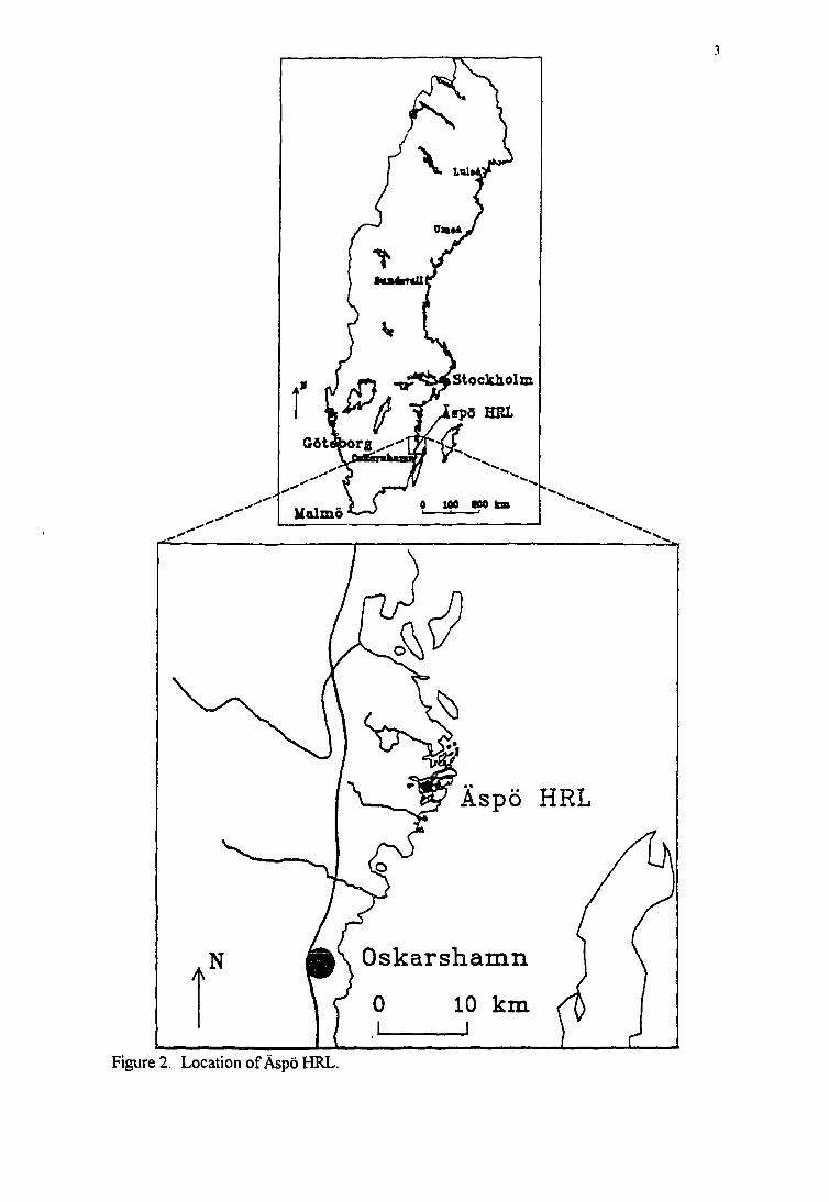
The Äspö Hard Rock Laboratory (HRL), which has been under construction since 1990, isapart of the SKB R & D program (The R & D program in Äspö Hard Rock Laboratory, HRL,Project is one of the efforts undertaken in order to prepare for the work at the candidate sites).The HRL will be placed at a depth of approximately 460 m below the island of Äspö, situatedabout 20 km north of the city of Oskarshamn in south eastern Sweden (Figure 2). The overallgoal of the SKB research program is to construct a safe repository for the nuclear waste.According to present plans the repository shall be ready for operation in 2020. The site of therepository shall be decided during the period 2003 - 2006. That decision will be preceded bypre-investigations at three sites and detailed investigations at two sites (Appendix 1).

The R&D work in the ÄSPÖ Hard Rock Laboratory (HRL) Project is one of the effortsundertaken in order to prepare for the work at the candidate sites. The main goals for theproject are:

* Test the quality and appropriatness of different methods for characterizing bedrock withrespect to conditions of importance for final repository.

* Refine and demonstrate methods for how to adapt a final repository to the localproperties of the rock in connection with planning and construction.

* Collect material and data of importance methods for the safety of the final repository andfor confidence in the quality of the safety assessments.

Stockholm

«fp« HEL

MalmöO 100 MO k a

Aspö HRL

Oskarshamn

0 10 kmi i

Figure 2. Location of Äspö HRL.

1.3 ECLIPSE program

ECLIPSE 100 is a fully - implicit black, three dimensional, general purpose black oil simulatorwith gas condensed options. The program is written in FORTRAN 77 and operates on anycomputer with an ANSI standard FORTRAN 77 compiler and either virtual storage orsufficient real storage. ECLIPSE 100 can be used to simulate 1, 2 or 3 phase systems. Twophase options (oil/water, oil/gas, gas/ water) are solved as two component systems saving bothcomputer storage and computer time. In addition to gas dissolving in oil (variable bubble pointpressure or gas/oil ratio), ECLIPSE may also used to model oil vaporizing in gas (variable dewpoint pressure or oil/gas ratio). In the next few pages YOU will see that ECLIPS5 has beenused for the first time in an attempt to model groundwater in a crushed zone.

Both standard blocks center and corner point Cartesian geometry can be used. The cornerpoint geometry option permits a faithful representation of reservoir geometry and the accuratecalculation of flow across sloping faults.

1.4 Aim of study

Much time and efforts can be spent on models which will yield only trivial answers to simpleproblems; if models are properly planned and provided with adequate data they can savevaluable time and money in addition to answering technical dilemmas.

ECLIPSE is one of the very modern programs in the field of oil production, but the programhas had little application to modeling groundwater.

The Äspö Hard Rock Laboratory (HRL) is a significant region to continued study of thebehavior of rocks and groundwater flow in Sweden.

The aim of this study is to try to model the groundwater flow in one of the most importantfractured zones in the HRL utilizing the multi-facility program, ECLIPSE.

The prosperity in this attempt means that the program become appropriate to model thegroundwater flow with different reservoir material. That means, in turn, it is then possible toimpose on that model future conditions which may develop, such as increased or redistributedpumping, increased or decreased production due to engineering surface structures, change inthe production patterns, or any other factors which may change the existing hydrogeologicalconditions.

2 OVERVIEW OF FIELD INVESTIGATION

The main purpose of this part of the report is to give an overview of the most important resultsof the field investigations, specially with respect to the interpretation and analyses of the datawhich formed the basis for the building of our model that will be presented later in this study.

2.1 GEOLOGY

2.1.1 Purpose of the investigation

The main aim of the geological investigations was to give a description on a regional of therock distribution and the structural pattern in the area.

2.1.2 Summarized presentation of main geological investigation data,interpretation and analysis

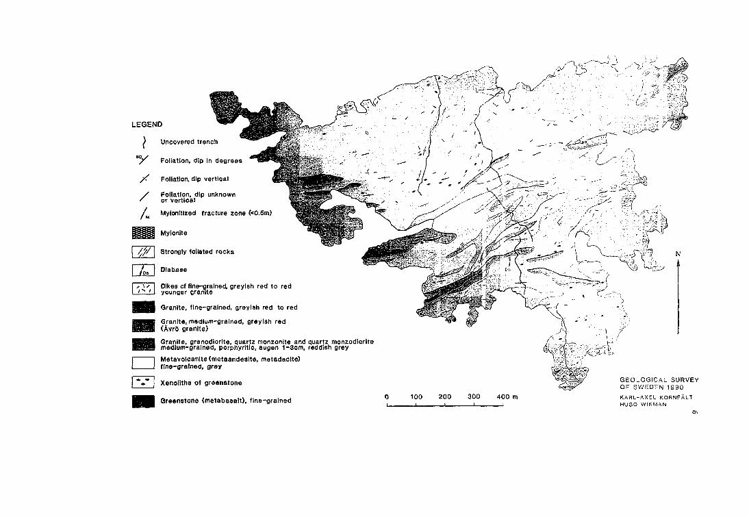
In order to get more detailed information about the geological conditions on Äspö a number ofgeological and geophysical studies were performed (Wikberg P et al 1991) (Figure 3).

The aim of the geological field study was to obtain information to make a description of thelithological distribution and petrological and structural characteristics of the different rocks onÄspö. Very detailed mapping was performed along cleaned trenches across the island, andgeological map to a scale of 1:2 000 was prepared (Wikberg P et al 1991). A classification ofthe rocks based on chemical and mineralogical analysis is presented.

A complementary study of structural elements including a fracture mapping program was alsoperformed along the cleaned trenches to obtain results for use in geohydrological and rockmechanics model studies. Data concerning 4500 mapped fractures - such as orientation, lengthaperture and fracture filling- is presented (Wikberg P et al 1991).

The main aim of the detailed geophysical investigation was to indicate fracture zones on Äspö,using mainly geomagnetic, geoelectric and seismic methods. Especially important was theinterpretation of dip of the fracture zones (Wikberg P et al 1991).

2.1.3 Lithology

The dominant rocks on Äspö belong to the 1700-1800 Ma Småland Granite suite, with maficenclaves and dikes probably formed in a continuous magma- mingling and magma mixingprocess.

The result of this mingling (mixing) process is a very inhomogenous rock mass, ranging inmineralogical composition from true granites to dioritic or gabbroic rocks. Rather largerirregular bodies of diorite/ gabbro have been located in boreholes at great depth in the sitearea.

LEGEND

) Uncovered trench

j y Foliation, dip In degrees

/ Foliation, dip vertical

/ Foliation, dip unknown' or vertical

/ , Mylonltized fracture zone («O.6m)

Mylonite

Strongly foliated rocks

L 4 J DiabaseI /• \* I Dikes of fine-grained, greyish red to redI **" ' I younger granite

Granite, fine-grained, greyish red to red

Granite, medium-grained, greyish red(Ävrö granite)

Granite, granodiorite, quartz monzonite and quartz monzodioritemedium-grained, porphyrltle, augen 1-3om, reddish grey

Metavolcanlte (metaandealte, metadacite)fine-grained, gray

Xenollths of greenstone

Greenstone (metabasalt), fine-grained 100 200 300 400 m

GEOLOGICAL SURVEYOF SVi/EDENi 1990KARL-AXEL KORNFÄLTHUGO WIKMAN

Older folded sheets of basic igneous rocks and xenoliths, often hybridized by the granitoids,are more or less dispersed in the rock mass, especially in the NE - ENE trending belt crossingcentral Äspö. Basic sheets tens of meters thick seem to have more gentle dips than sheets onlyabout one meter thick.

All the rock mass in Äspö is intruded by the 1300 -1400 Ma Götemar Granite, which are fine-grained granites of at least two or three generations, related to the Småland Granite. The fine-grained granites form dikes of different widths - often trending NE and almost vertical- butalso very irregular masses and veins which have been found by coring at different depths.

Based on surface observations and drill core logging, a particle classification limit was laterfixed at the silicate density 2.65 - 2.70 g/cm3 between what is now called Småland Granite andÄspö Diorite. The most basic variant observed in some boreholes in Äspö, with silicate densityabove 2.75 g/cm3, is assigned to the Greenstone Group,

In small areas on southern Äspö a redder variety of the Småland Granite is observed. Thisrock, which is called Ärvö Granite, is a true granite with rather small microcline rnegacrystswhich are sparsely scattered compared with the porphyritic granitoids.

Across the island of Äspö, from SW to NE, there are a number of outcrops with grayish black,fine grained basic rocks with a basaltic composition. They are very often strongly altered andcalled greenstone. Gray to dark - gray fine - grained with a dactylic composition onlyconstitute minor parts of the Äspö island. Most of these metavolcanic rocks seem to be olderthan the Småland Granite, based on the fact that they form thin sheets and xenoliths ingranitoid. Along the border between the medium- grained granitoid and greenstone, there aresometimes accumulation of fine- grained grayish- grained- red granite.

Fine - grained granite also occurs frequently on Äspö as more or less well- defined dikes orveins intersecting the older rocks. The width of the often NE trending dikes is normally fromone decimeter to some meters, but there are also wider dikes of this rock - up to 25 metersacross. These fine - grained granites can be classified as true granites.

Most of the fine - grained granites on Äspö seem to be an organic and related to the 1300-1400 Ma Götemar - Uthammar Granite, but there is certainly also at least one generation offine- grained granite related to the older Småland granitiods.

Aplite and pegmatite as well as diabase have only been observed as very narrow dikes seldommore than a few decimeters wide.

2.1.3 Fracture mapping

The mapping has mainly been done on outcrops following the two cleaned N-S profiles onÄspö island. The principal aim of the fracture mapping measurements was to produce resultsfor geohyrological and rock mechanics model studies (Wikberg P et al 1991).

Summarized rosette diagram shows dominating sectors around N 60°W, N 5° and N 60° E. E-W fractures are more scare but still occur in a narrower, prominent peak (Figure 4) . About85% of 4500 mapped fractures are steep, with dips in the range 70°- 90°.

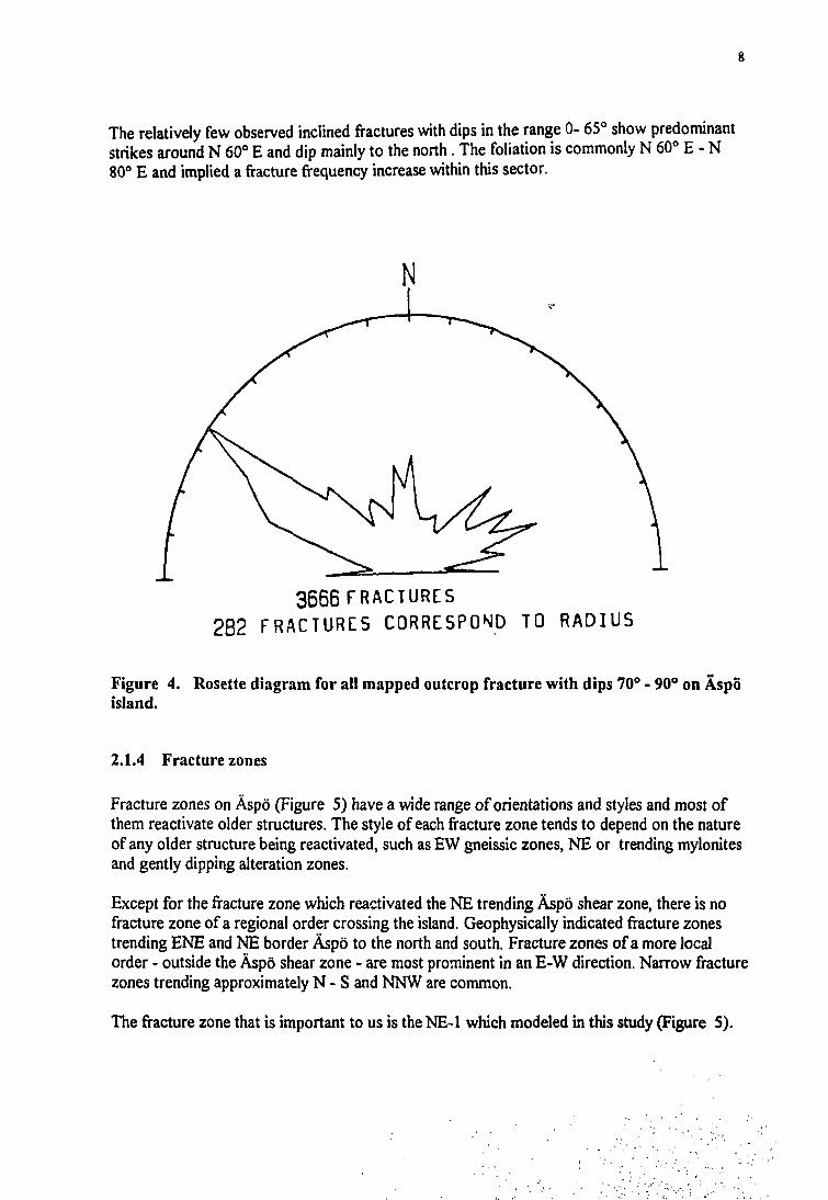
The relatively few observed inclined fractures with dips in the range 0- 65° show predominantstrikes around N 60° E and dip mainly to the north. The foliation is commonly N 60° E - N80° E and implied a fracture frequency increase within this sector.

3666 FRACTURES2B2 FRACTURES CORRESPOND TO RADIUS

Figure 4. Rosette diagram for all mapped outcrop fracture with dips 70° - 90° on Äspöisland.

2.1.4 Fracture zones

Fracture zones on Äspö (Figure 5) have a wide range of orientations and styles and most ofthem reactivate older structures. The style of each fracture zone tends to depend on the natureof any older structure being reactivated, such as EW gneissic zones, NE or trending mylonitesand gently dipping alteration zones.

Except for the fracture zone which reactivated the NE trending Äspö shear zone, there is nofracture zone of a regional order crossing the island. Geophysically indicated fracture zonestrending ENE and NE border Äspö to the north and south. Fracture zones of a more localorder - outside the Äspö shear zone - are most prominent in an E-W direction. Narrow fracturezones trending approximately N - S and NNW are common.

The fracture zone that is important to us is the NE-1 which modeled in this study (Figure S).

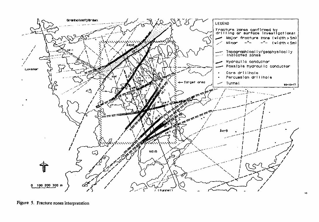
LEGEND

Fracture zones conftrmed bydrilling or surface Invest Iaa+lons:

Major fracture zone (width>5m)Minor -"- -"- (width <5m)

-- Topograph1ca11y/geophyaleal IyIndicated zones

Hydraulic conductorPossible hydraulic conductor

Core drlI I holePercussion drillholeTunnel „_,„_„ '

Figure 5. Fracture zones interpretation

10

2.1.5 Borehole investigations

During the investigation, a drilling program was executed at different stages comprising 14cored borehole and a number of percussion borehole in the Äspö area. In addition, a largenumber of boreholes- mostly percussion boreholes - were also sighted in the surrounding area(WikbergPetall991).

The aim of the boreholes was to obtain basic information on the bedrock composition,orientation and characteristics of the major fracture zone and hydraulic properties of the rockmass at increasing depth.

When drilling was finished a great number of different investigation methods were used in theborehole and the drilled core were mapped and investigated in a great detail.

Observations of water movement and temperature signatures in the boreholes were obtainedmainly from temperature measurements and borehole fluid - resistivity logs. Water transport inthe borehole is common and occurs when the borehole serves as a connection between waterbearing fracture/ fracture zones with different hydraulic heads.

2.2 GEOHYDROLOGY

2.2.1 Purpose of investigation

The purpose of investigation was to describe the natural groundwater distribution and flow in aselected rock volume. Of particular interest is the description of the geometric distribution ofthe groundwater flow in the rock volume and the quantification of transmissivity and pressurehead in these volumes, zones or fractures. A further goal of the investigations was to supplythe data necessary for setting up mathematical groundwater models for a selected rockvolume.

2.2.2 Summarized presentation of main geohydrological data

The island Äspö is situated on the eastern coast of southern Sweden. Despite the coastalposition, the climate is governed by the prevailing westerly winds, which are comparativelydry. The total mean precipitation is 675 mm/year. The average temperature in Oskarshamn is6.4 °C, with February as the coldest month, -2.9 °C, and July as wannest, 16.2 °C. Of theannual precipitation, about 125 mm/year falls as snow, and the durability of the snow cover ison average 91 days. The total evapotranspiration is calculated to be 490 mm/year, leaving arun off of 150 - 200 mm/year.

The groundwater levels in the area are at maximum in the spring, during the snow melt period.At a distance from the coast, winter minimum levels may occur, but the annual absoluteminimum is the summer one. The annual recharge has estimated to be 128 to 218 mm/year inpervious ground. The groundwater level was found to be 8 -10 m below ground level.

11

Measurements made near the existing facilities show that these have only a small influence onthe level fluctuations. The natural fluctuation of the water level during a year is expected to beless than about 1 m. In some boreholes the water level may rise up to 1 m during a few days orweeks if the precipitation is large. The maximum water level on Äspö is about + 4 m.

Interference pumping tests were performed in the boreholes with higher yields. Analysis ofthese data showed transmissivities as high as T = 3.3 x 10"4 m2/ s at Äspö (Wikberg P et al1991).

During 1987 -1989, the levels of the Baltic sea ranged from - 0.5 to + 0.8 m above sea level,with normal fluctuation within ± 0.3 m.

The conclusion that one can get from the result of the pumping test in the 13 boreholes inÄspö is that the average hydraulic conductivity is ranged between 1.6 x 10"8 to4.5 x 10-6 m/s (Wikberg P et al 1991).

12

THE FRACTURE ZONE NE-1

3.1 BACKGROUND AND PURPOSE

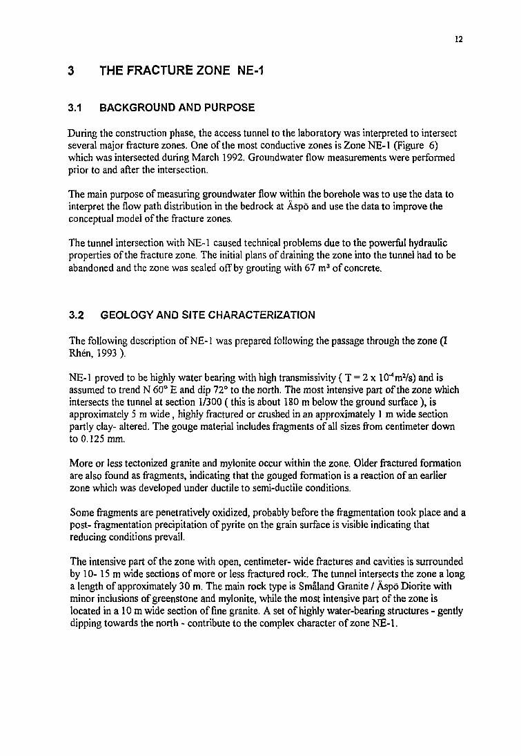
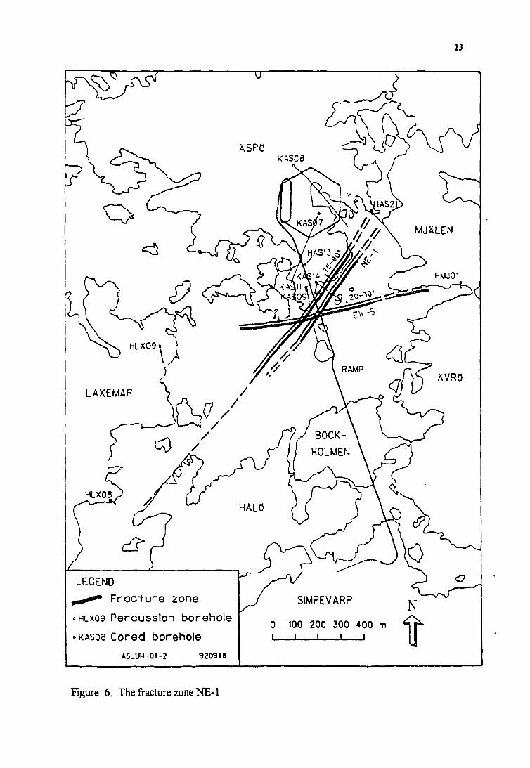
During the construction phase, the access tunnel to the laboratory was interpreted to intersectseveral major fracture zones. One of the most conductive zones is Zone NE-1 (Figure 6)which was intersected during March 1992. Groundwater flow measurements were performedprior to and after the intersection.

The main purpose of measuring groundwater flow within the borehole was to use the data tointerpret the flow path distribution in the bedrock at Äspö and use the data to improve theconceptual model of the fracture zones.

The tunnel intersection with NE-1 caused technical problems due to the powerful hydraulicproperties of the fracture zone. The initial plans of draining the zone into the tunnel had to beabandoned and the zone was sealed off by grouting with 67 m3 of concrete.

3.2 GEOLOGY AND SITE CHARACTERIZATION

The following description of NE-1 was prepared following the passage through the zone (IRhen, 1993).

NE-1 proved to be highly water bearing with high transmissivity ( T = 2 x lO^nWs) and isassumed to trend N 60° E and dip 72° to the north. The most intensive part of the zone whichintersects the tunnel at section 1/300 (this is about 180 m below the ground surface ), isapproximately 5 m wide, highly fractured or crushed in an approximately 1 m wide sectionpartly clay- altered. The gouge material includes fragments of all sizes from centimeter downto 0.125 mm.

More or less tectonized granite and mylonite occur within the zone. Older fractured formationare also found as fragments, indicating that the gouged formation is a reaction of an earlierzone which was developed under ductile to semi-ductile conditions.

Some fragments are penetratively oxidized, probably before the fragmentation took place and apost- fragmentation precipitation of pyrite on the grain surface is visible indicating thatreducing conditions prevail.

The intensive part of the zone with open, centimeter- wide fractures and cavities is surroundedby 10-15 m wide sections of more or less fractured rock. The tunnel intersects the zone a longa length of approximately 30 m. The main rock type is Småland Granite / Äspö Diorite withminor inclusions of greenstone and mylonite, while the most intensive part of the zone islocated in a 10 m wide section of fine granite. A set of highly water-bearing structures - gentlydipping towards the north - contribute to the complex character of zone NE-1.

13

K^py\ //

/A^A<h ^

LEGEND

Frac+ure zone

»HLX09 Percussion borehole

'KAS08 Cored boreholeAS_UH-O1-2 92091B

Figure 6. The fracture zone NE-1

14

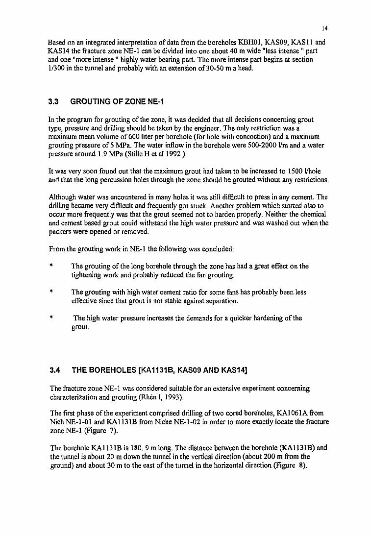
Based on an integrated interpretation of data from the boreholes KBH01, KAS09, KAS11 andKAS14 the fracture zone NE-1 can be divided into one about 40 m wide "less intense " partand one "more intense" highly water bearing part. The more intense part begins at section1/300 in the tunnel and probably with an extension of 30-50 m a head.

3.3 GROUTING OF ZONE NE-1

In the program for grouting of the zone, it was decided that all decisions concerning grouttype, pressure and drilling should be taken by the engineer. The only restriction was amaximum mean volume of 600 liter per borehole (for hole with concoction) and a maximumgrouting pressure of 5 MPa. The water inflow in the borehole were 500-2000 l/m and a waterpressure around 1.9 MPa (Stille H et al 1992).

It was very soon found out that the maximum grout had taken to be increased to 1500 I/holeand that the long percussion holes through the zone should be grouted without any restrictions.

Although water was encountered in many holes it was still difficult to press in any cement. Thedrilling became very difficult and frequently got stuck. Another problem which started also tooccur more frequently was that the grout seemed not to harden properly. Neither the chemicaland cement based grout could withstand the high water pressure and was washed out when thepackers were opened or removed.

From the grouting work in NE-1 the following was concluded:

* The grouting of the long borehole through the zone has had a great effect on thetightening work and probably reduced the fan grouting.

* The grouting with high water cement ratio for some fans has probably been lesseffective since that grout is not stable against separation.

* The high water pressure increases the demands for a quicker hardening of thegrout.

3.4 THE BOREHOLES [KA1131B, KAS09 AND KAS14]

The fracture zone NE-1 was considered suitable for an extensive experiment concerningcharacterization and grouting (Rhen I, 1993).

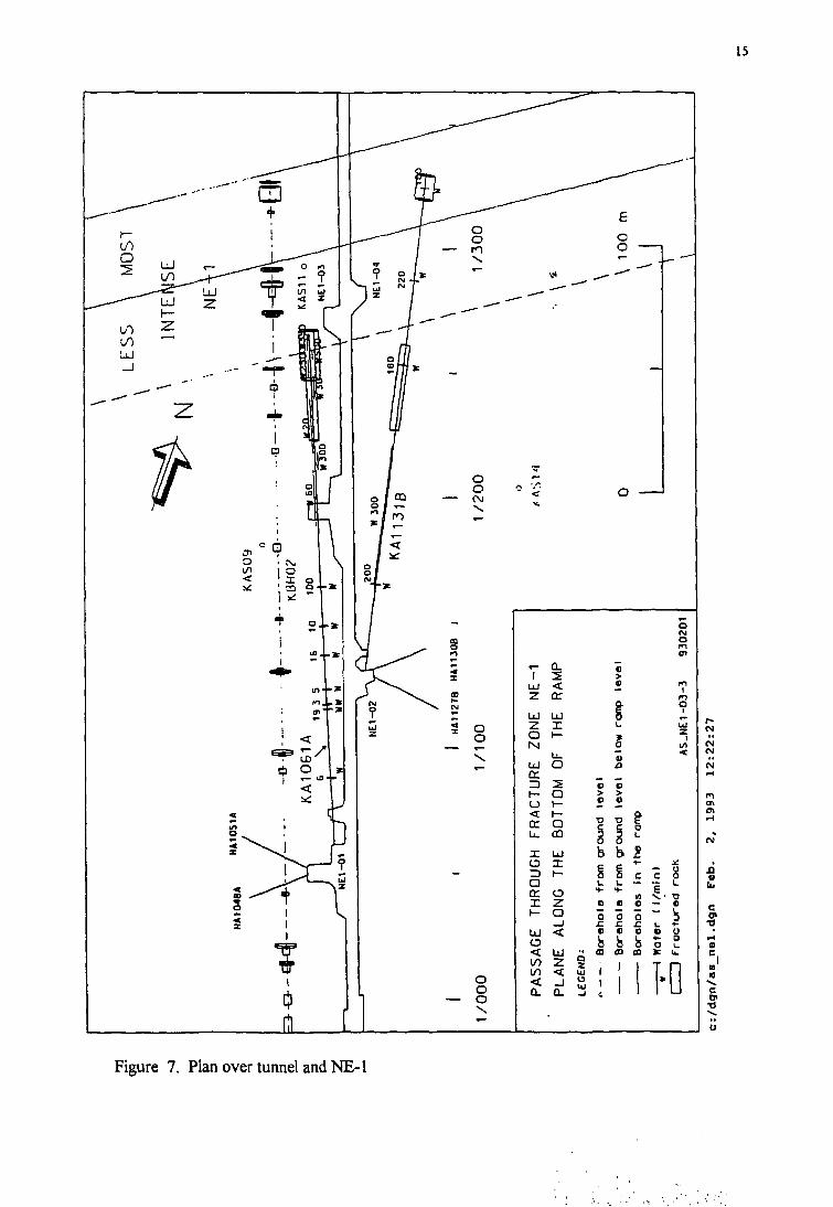
The first phase of the experiment comprised drilling of two cored boreholes, KA1061A fromNich NE-1-01 and KA113 IB from Niche NE-1-02 in order to more exactly locate the fracturezone NE-1 (Figure 7).

The borehole KA113 IB is 180. 9 m long. The distance between the borehole (KA113 IB) andthe tunnel is about 20 m down the tunnel in the vertical direction (about 200 m from theground) and about 30 m to the east of the tunnel in the horizontal direction (Figure 8).

15

OJCM

en

c c 8I. U — •- Lt- H- E

10 v. • T3O o o — oö ö ö " iC O C C O

O ö O O uO O <D K u.I 1-D

•o

o

a

13

Figure 7. Plan over tunnel and NE-1

16

The borehole KAS09 is about 450 m long and 0.056 m in diameter, and the inclination is about60° to the horizontal plane.

The borehole KAS14 is about 212 m long and 0.056 m in diameter, and the inclination is about61° to the horizontal plane.

The aim of drilling KAS09 and KAS14 was to penetrate NE-1 to identify its location andhydraulic properties. The pumping test in these boreholes indicated a conductive structure withhigh transmissivity. According to a spinner survey, the structure comprised two parts, NE-1 aand NE-lb, both of which probably have a dip of approximately 70° N.

KA106U

Figure 8. Vertical section perpendicular to NE-1.The broken line is assumed to represent NE-1

17

3.5 TRACER TEST

3.5.1 Tracer used

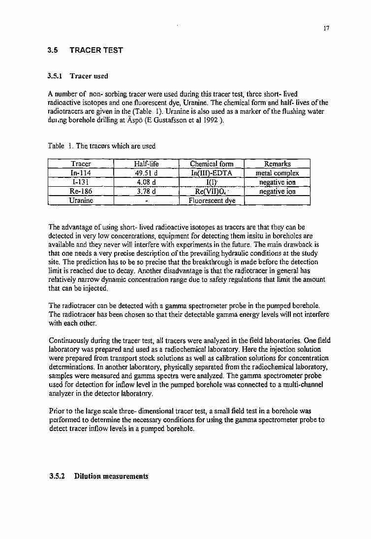
A number of non- sorbing tracer were used during this tracer test, three short- livedradioactive isotopes and one fluorescent dye, Uranine. The chemical form and half- lives of theradiotracers are given in the (Table 1). Uranine is also used as a marker of the flushing waterdunng borehole drilling at Äspö (E Gustafsson et al 1992 ).

Table 1. The tracers which are used

TracerIn-1141-131

Re-186Uranine

Half-life49.51 d4.08 d3.78 d

-

Chemical formIn(III)-EDTA

Re(VH)O< •Fluorescent dye

Remarksmetal complex

negative ionnegative ion

The advantage of using short- lived radioactive isotopes as tracers are that they can bedetected in very low concentrations, equipment for detecting them insitu in boreholes areavailable and they never will interfere with experiments in the future. The main drawback isthat one needs a very precise description of the prevailing hydraulic conditions at the studysite. The prediction has to be so precise that the breakthrough is made before the detectionlimit is reached due to decay. Another disadvantage is that the radiotracer in general hasrelatively narrow dynamic concentration range due to safety regulations that limit the amountthat can be injected.

The radiotracer can be detected with a gamma spectrometer probe in the pumped borehole.The radiotracer has been chosen so that their detectable gamma energy levels will not interferewith each other.

Continuously during the tracer test, all tracers were analyzed in the field laboratories. One fieldlaboratory was prepared and used as a radiochemical laboratory. Here the injection solutionwere prepared from transport stock solutions as well as calibration solutions for concentrationdeterminations. In another laboratory, physically separated from the radiochemical laboratory,samples were measured and gamma spectra were analyzed. The gamma spectrometer probeused for detection for inflow level in the pumped borehole was connected to a multi-channelanalyzer in the detector laboratory.

Prior to the large scale three- dimensional tracer test, a small field test in a borehole wasperformed to determine the necessary conditions for using the gamma spectrometer probe todetect tracer inflow levels in a pumped borehole.

3.5.2 Dilution measurements

18

Before the tracer injection started, dilution measurements were performed in six candidateborehole sections to find the four best for the tracer injections. Then, during the first part ofthe tracer test, additional dilution measurements were made in four new borehole to findsections suitable for the large tracer pulse injections at the end of the test.

Dilution measurements were performed for determination of groundwater flow throughboreholes or packed- off sections (hydraulic units) of boreholes. The groundwater flow wasusually calculated as a mean value over a period of a few days in a borehole section limited byborehole packers. The borehole section lengths at Äspö varied from about 30 to 100 m. Thedilution (circulation) section in the bore was connected to the ground surface with two plastictubes, as shown in (Figure 9). The downward tube outlet was situated at the bottom of thesection and the inlet at the top. The circulation pumps placed in the near surface PEM tubeestablished a circulation system where the groundwatcr in the borehole section was mixed.

The amount of the tracer was constantly added during one circulation cycle to the circulatingwater system. This tracer must posses the quality that it can be added to the studied water ineither low or high concentrations and then still be possible to detect in very low concentrationi.e. a wide concentration.

The tracer concentration in the borehole section then decreased as the through flowinggroundwater diluted the section of tracer labeled water. The dilution of the tracer in the wateris proportional to the groundwater flow through the section.

As the amount of the injected tracer solution was usually limited for four or five hours, thetracers will not be forced out into the fracture system with excess pressure. If the fracture isjudged to have a low hydraulic conductivity, it is possible to withdraw the same amount ofwater from the circulating system as is injected.

The groundwater flow through the borehole sections is generally determined with an error lessthan a few percent. If the flow rate through the borehole section is to be converted togroundwater flow in the straddled fracture zone, some factors that may cause errors in thecalculated value have to be considered. The disturbance in the flow field due to the presence ofthe borehole and the presence of the several water conducting fractures within the measuredsection may provide short-circuits between the fracture (with different hydraulic head)resulting in enhanced flow rates. The flow in the fracture has spatial differences due to unevendistribution of fracture apertures and other heterogeneity. Consequently, if a boreholepenetrates a highly conductive fracture in a location where the fracture surfaces are in contactwith each other, it will show lower values of groundwater flow than if the borehole hadpenetrated a "flow channel" in the fracture. Also angle between the borehole and the fracturezone, as well as the direction of groundwater flow has to be considered in that case.

19

True elementunit

Pressureregulatorforboreholepackers

£. pressure registration

Circulation pump

Groundwaterpressureregistration

Boreholepackers

Dilution section

• Outlet from trace element unit

' Inlet to circulation pump

Figure 8. Schematic of injection borehole equipment (Rhen I et al 1992).

20

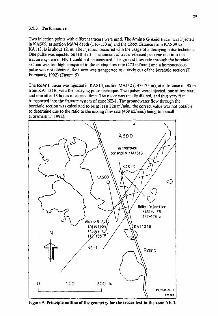
3.5.3 Performance

Two injection points with different tracers were used. The Amino G Acid tracer was injectedin KAS09, at section MA94 depth (116-150 m) and the direct distance from KAS09 toKAl 13 IB is about 121m. The injection occurred with the usage of a decaying pulse technique.One pulse was injected on test start. The amount of tracer released per time unit into thefracture system of NE-1 could not be measured. The ground flow rate through the boreholesection was too high compared to the mixing flow rate (273 ml/min.) and a homogeneouspulse was not obtained, the tracer was transported to quickly out of the borehole section (TForsmark, 1992) (Figure 9).

The RdWT tracer was injected in KAS14, section MA142 (147-175 m), at a distance of 92 mfrom KAl 13 IB, with the decaying pulse technique. Two pulses were injected, one at test startand one after 18 hours of elapsed time. The tracer was rapidly diluted, and thus very fasttransported into the fracture system of zone NE-1. The groundwater flow through theborehole section was calculated to be at least 328 ml/min., the correct value was not possibleto determine due to the ratio to the mixing flow rate (468 ml/min.) being too small(Forsmark T, 1992).

0I

Withdrowolborehole KA1131B

RdWt Inject ionKAS14. F8147-175 m

AS.THAC-01-1

321203

Figure 9. Principle outline of the geometry for the tracer test in the zone NE-1.

21

3.5.4 Results

The recovery of RdWT in the withdrawal borehole KA113IB was 3.7 %o during the 44 hourinterference test, February 14-16, 1992. The calculation is based on a withdrawal flow rate of3711/min. (534.24 m3/day). Since only the ascending part of the tracer break-through curvewas obtained during the limited interference test, the borehole was opened on nine occasionsduring the period February 21 to March 10, which gave an additional recovery of 7.6 %o(Forsmark T, 1992).

According to the observation in the tunnel, it seems possible that there was a leakage of 100-3001/min. into the tunnel front during the period February 14 to March 10. This inflow wasnot sampled for a tracer content test (Rhen I et al 1993).

Amino G Acid was not recovered in the samples from KA113 IB during the interference test(February 14-16 1992), or during the period February 21 to March 10. Also it was notrecovered in the samples taken later from percussion boreholes and nor from inflow to thetunnel.

In summary, the measured recovery until March 19 was 1.13% of RdWT and 0 % of Amino GAcid.

Depending on model assumptions for the inverse modeling, the mean travel time (t.) for RdWTwas estimated at 56 or 82 hours. It was not possible to estimate the mean travel time forAmino G Acid, but was also used for estimating the flow porosity (Rhen I et al 1993).

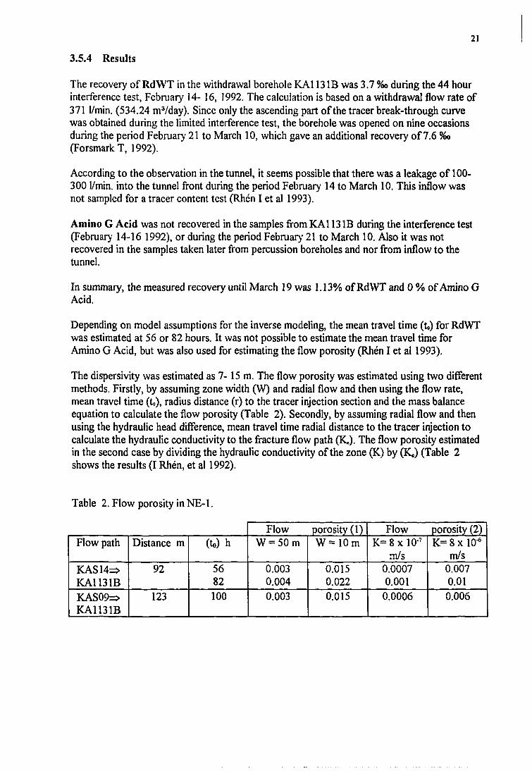
The dispersivity was estimated as 7-15 m. The flow porosity was estimated using two differentmethods. Firstly, by assuming zone width (W) and radial flow and then using the flow rate,mean travel time (t>), radius distance (r) to the tracer injection section and the mass balanceequation to calculate the flow porosity (Table 2). Secondly, by assuming radial flow and thenusing the hydraulic head difference, mean travel time radial distance to the tracer injection tocalculate the hydraulic conductivity to the fracture flow path (K«). The flow porosity estimatedin the second case by dividing the hydraulic conductivity of the zone (K) by (IQ (Table 2shows the results (I Rhen, et al 1992).

Table 2. Flow porosity in NE-1.

Flow path

KAS14=>KA1131BKAS09=>KA1131B

Distance m

92

123

(to)h

5682100

FlowW = 50m

0.0030.0040.003

porosity (1)W=10m

0.0150.0220.015

FlowK= 8 x 10-7

m/s0.00070.0010.0006

porosity (2)K= 8 x 10"6

m/s0.0070.010.006

22

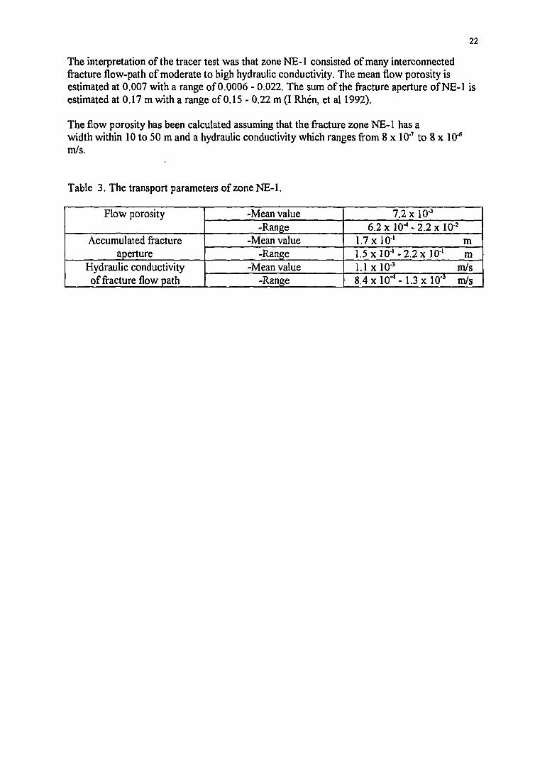
The interpretation of the tracer test was that zone NE-1 consisted of many interconnectedfracture flow-path of moderate to high hydraulic conductivity. The mean flow porosity isestimated at 0.007 with a range of 0.0006 - 0.022. The sum of the fracture aperture of NE-1 isestimated at 0.17 m with a range of 0.15 - 0.22 m (I Rhen, et al 1992).

The flow porosity has been calculated assuming that the fracture zone NE-1 has awidth within 10 to 50 m and a hydraulic conductivity which ranges from 8 x 10'7 to 8 x 10"6

m/s.

Table 3. The transport parameters of zone NE-1.

Flow porosity

Accumulated fractureaperture

Hydraulic conductivityof fracture flow path

-Mean value-Range

-Mean value-Range

-Mean value-Range

6.:1.7 x1.5 x1.1 X8.4 x

7.2 x 10-3

Ix 10-"-2.2x K10'10"'-2.2x10"'io-3

l O ^ - U x 1O'J

)2

mm

m/sm/s

23

ECLIPSE SIMULATION

4.1 ECLIPSE AS COMPATIBLE PROGRAM

ECLIPSE 100 is known as a fully implicit black oil simulator with a wide range of modelingfacilities. The familiar usage for ECLIPSE 100 is as an oil simulator, even when the programcan be used to simulate 1,2 or 3 phases, it means with one phase option just black oil, for twophase option oil/gas and for three phase option oil/gas/water thus it is the novel to useECLIPSE 100 as just a groundwater simulator.

The programs INTERAVEW and GRAF are connected with ECLIPSE 100 to show resultsfrom the simulation.

INTERAVIEW is used to show the reservoir with its properties in a color 3-D figures.

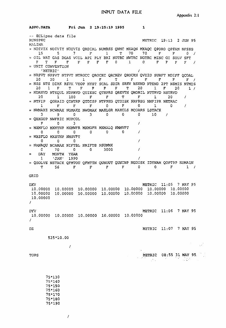
4.2 INPUT DATA

An ECLIPSE data input file is split into sections, each of which is introduced by a keyword. Alist of all these sections and the keywords which belong to each section, together with a briefdescription of the contents of each section, keyword respectively is given below. Eachdescription is followed by and calculations about the values that we used in our case(Appendix 2).

/ . RUNSPEC Is the first section of an ECLIPSE data input file. It contains the run title,start date, units, various problem dimensions (number of blocks, wells,tables, etc.) (Appendix 2:1).

THE MODEL The unites are metric. In our case, we use 525 grid blocks (cells),three wells, 70 non - neighbor connections, one table for PVT etc.

2. GRID Defines the geometry of the computational grid and rock properties (thedepth, porosity, permeability, net to gross ratio) in each grid block (cell).

DVX Vector of X direction grid block sizes.

THE MODEL 15 grid blocks in the X direction, each grid block is 10 m long(Appendix 2:1).

DVY Vector of Y direction grid block sizes.

THE MODEL 5 grid blocks in the Y direction, each grid block is 10 m long(Appendix 2:1).

DZ Vector of Z direction grid block sizes.

THE MODEL 7 grid blocks in the X direction, each grid block is 10 m deep(Appendix 2:1).

24

TOPS

THE MODEL

PORO

THE MODEL

PERMX &PERMY

Depths of top faces of the grid blocks in the current input box.

The depth for our model is between 130 to 200 m, and was controlled by thedepth of the tunnel and the borehole are passing through the crushed zone(Appendices 2:1 and 3).

Grid blocks properties for the current input box.

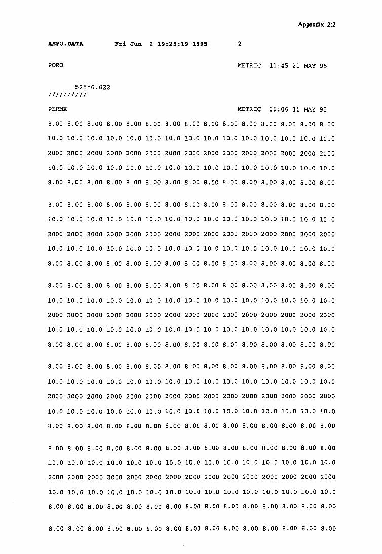
The porosity in our case ranges between 0.022- 0.00062. We use0.022 for all the grid blocks in the model (Appendix 2:2).

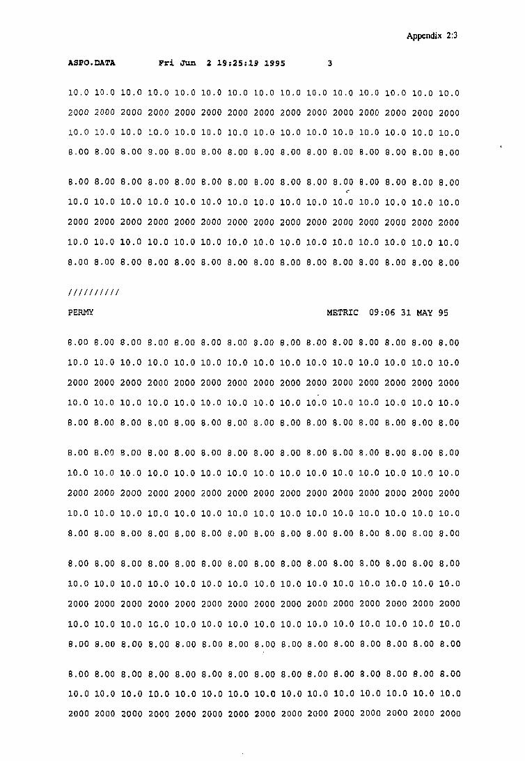
X & Y directions permeability for the current input box.

THE MODEL The values units should be in millidarcy where:

1 millidarcy (md) gives 0.966x IP8 & 1 x 70"* m/s.

As we showed above, the hydraulic conductivity ranges between 8 x 10'7 to8 x 10"6 m/s which means between 80 - 800 md. But the hydraulicconductivity in the flow path is very high (between 8.4x10 -1.3 x 10'3 m/sor 84 000 -130 000 md) and so we use the high values at the middle andgradually decrease towards the edges. Our values are 2000 md in the middlegrid blocks and 10 md at the grid blocks between the middle and the edgesand 8 md at the edges (Appendices 2:4-5 and 4).

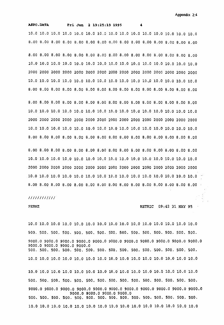
PERMZ

THE MODEL

Z direction permeability's for the current input box.

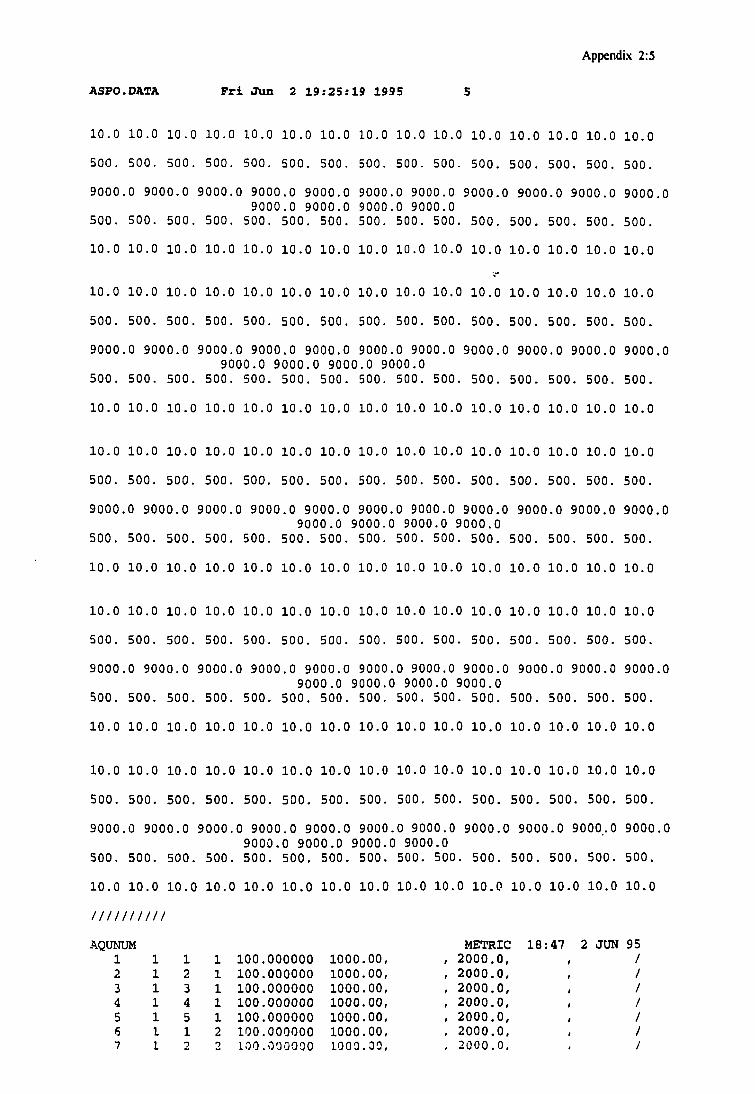
The same principles for the permeability in the X & Y directions areimplemented in the Z direction, but the values at the middle grid blocks arehigher by 4.5 times than the values in the both the X & Y directions. In otherwords, the permeability values in the middle grid blocks are 9000 md, and inthe grid blocks between the middle and the edges are 500 md, and at theedges are 10 md (Appendices 2:4-5 and 5).

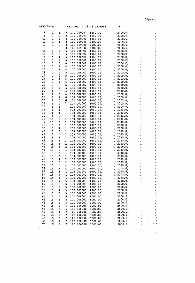
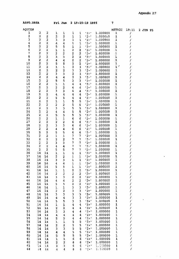
AOUNUM Defines the connection between the numerical aquifer and the reservoir.

AQUNUM Defines a numerical aquifer.

THE MODEL

OLDTRAN

The above two keywords are required for a numerical aquifer. In ourcase, this connection happens at the both edges in the X direction with 35grid blocks at each edge. These grid blocks are called non-neighborconnection grid blocks. (Appendix 2:5-8).

Specifies that block centered data should be used to compute thetransmibilities.

Produces Initial File for GRAF.

THE MODEL The last two keyword do not need input data (Appendix 2:8).

RPTGRID Sets report levels for GRID data.

25

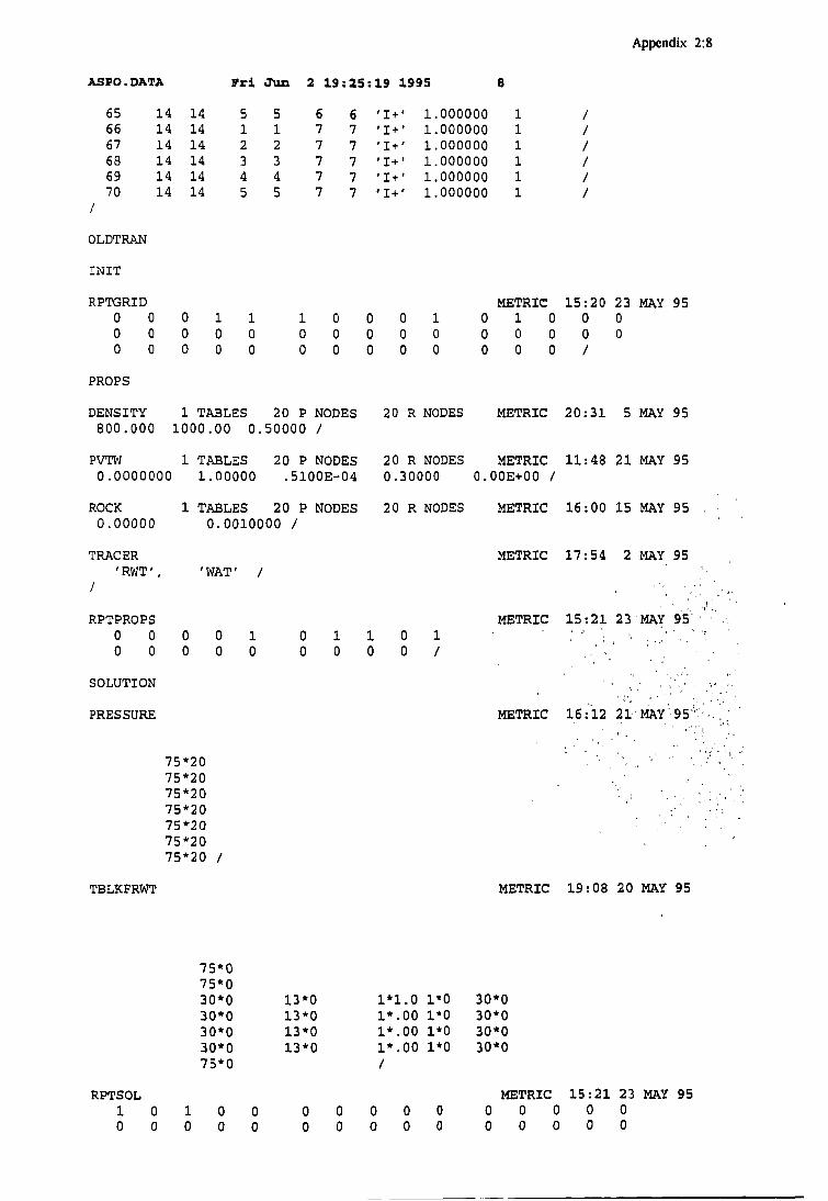
3. PROPS The section contains pressure, composition and saturation dependentproperties of the reservoir fluids and rocks (Appendix 2:8).

DENSITY Stock tank fluid densities.

OUR MODEL The density value that we used is 1000 kg/m3 (Appendix 2:8).

PVTW In this keyword, one will give the compressibility and viscosity.

OUR MODEL (Appendix 7) shows the connection between the temperature, watercompressibility and water viscosity. We assume that the groundwatertemperature is about 10 °C and from the Table in (Appendix 6:2) thecompressibility is 4.78 x 10 '5 BARS *' . The viscosity value that we use isless than the value from the diagram in (Appendix 6:1), and is required justto make the program run and to avoid the shutting in of wells (Appendix2:8).

ROCK This keyword concerns the rock compressibility.

OUR MODEL According to the table below, the compressibility for the rock is in our caselxlO"3 BARS"1 (Appendix 2:8).

Table 4.ClaySandGravelJointedSound

The compressibility of different kinds

rockrock

0.1-0.0010.01 - 0.00010.001 - 0.000010.001 - 0.000010.0001 - 0.000001

ofrocksBARS1

BARS1

BARS1

BARS1

BARS'

TRACER Names and phases of passive tracers.

OUR MODEL " RWT " is the abbreviation name of our tracer and the phase is water(Appendix 2:8).

RPTPROPS Report levels for PROPS data.

4. SOLUTION This section contains data to define the initial state (pressure andsaturation) of every grid block in the reservoir. This data may take any oneof the following forms:

1-Equilibration

2-Restart

3-Enumeration.

26

OUR MODEL We chose the Enumeration as a suitable alternative for our case. Tochose this alternative, the user may specify the initial solution forevery grid block using the keywords :

1-PRJESSURE.

2-SWAT, SGAS.

3-RS or PBUB.

4-RV or PEDW.

The water is the only phase in our model and the program protested at theuse of the keyword SWAT unless more than one phase is used.

PRESSURE This keyword shows the initial pressure in every grid block.

OUR MODEL The pressure was measured in the boreholes to 1.9 MPa = 19 BARS.We use 20 BARS to make the run of the program easier (Appendix 2:8).

TBLKFRWT Initializes concentration of tracer concentration in every grid block.

OUR MODEL The experiment of the tracer test in the borehole KAS14 shows that thetracer RdWT was injected in KAS14, section MA142 (147-175 m depth).In our program, the location is 150 m depth and the concentration is 100% atthat depth (Appendix 2:8).

RPSTOL Report switches for SOLUTION data (Appendix 2:8).

5. SUMMARY The section specifies a number of variables which are to be written tosummary files after each time step of the simulation (Appendix 2:8).

6. SCHEDULE This section specifies the operations to be simulated ( production andinjection controls and constrains) and the times at which output reportsrequired.

The order in which keywords are specified in the SCHEDULE sectiondictates the order in which the specified operation simulated.

WELSPECS Introduces new wells and specifies some of their data.

OUR MODEL In this keyword, we defined the boreholes by names as follows :

-KAS14 = ' INJC'.

-KA1131Bs 'PROD1.

-The Tunnel =' TUNL'.

COMDAT

OUR MODEL

WCONHIST

27

We also define the location of the well head in the X-Y plane and thepreferred condition of the wells (i.e. allowing or preventing the crossflow,the well acts as one- way valve) (Appendix 2:10).

The data in this keyword defines the connection between wells and thereservoir.

The well in ECLIPSE defines as a vertical well, but in our case thetunnel and the borehole KAl 13 IB are stretching horizontally. Tointroduce the horizontal tunnel and borehole KAl 13 IB have we definedthem through the grid blocks in the horizontal direction and then we shutdown the grid blocks in the vertical direction above both the tunnel and theborehole KAl 13 IB to prevent the leakage in these grid blocks (Appendix2:10).

One of the compulsory keywords which observes production rates forHistory Matching Wells. Either WCONPROD or WCONHIST must be usedto specify production wells once they have been introduced withWELSPECS and COMPDAT.

OUR MODEL The withdrawal flow rate from borehole KAl 13 IB is about 371 1/min.(534.24 m3/day), and at the same time the leakage from in the tunnel fronthad been estimated to 100 - 3001/ min. (144 - 432 m3/day) (Appendix 2:11).

We use this keyword two times. Firstly, for 44 hours or almost two days (we define that later in the keyword TSTEP which is also used two times)based on the duration the water pumping. We use 534.24 m3/day aswithdrawal flow rate from the borehole KAl 13 IB and the leakage was 144m3/day.

Secondly, for 6 days which is the period that the recovery in the boreholeKAl 13 IB would need. The leakage in the tunnel front was the only flow ratethat we defined the second time, but the flow rate was higher this time 195mVday (which is logical).

RPTSCHED Report switches for simulation results (Appendix 2:11).

TUNING Time step limits, error tolerances and iteration limits.

WFHSTCTL This keyword is optional and we used it to set control mode instructionsfor all History Matching wells (Appendix 2:11).

TSTEP This keyword introduces the interval(s) to next report time(s).

WCONHIST See WCONHIST above.

TSTEP See TSTEP above.

END The keyword terminates the simulation.

28

4.3 INTERAVIEW

INTERAVIEW Is an interactive 3-D visualization system which may be used to displayreservoir simulation model input and output.

We have used this system to show some properties for our program for example thepermeability in X, Y an Z directions (Appendix 3, 4 and 5).

The reason that we did not get the heads of the wells may be that the model is not stretching toground surface.

29

RESULTS AND DISCUSSION

This study is an attempt to model the groundwater flow in the fracture zone NE-1 with usingof ECLIPSE program.

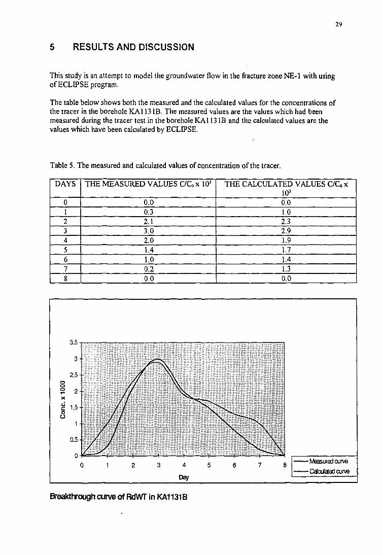
The table below shows both the measured and the calculated values for the concentrations ofthe tracer in the borehole KAl 13 IB. The measured values are the values which had beenmeasured during the tracer test in the borehole KAl 13 IB and the calculated values are thevalues which have been calculated by ECLIPSE.

Table 5. The measured and calculated values of concentration of the tracer.

DAYS

012345678

THE MEASURED VALUES C/Co x 103

0.00.32.13.02.01.41.00.20.0

THE CALCULATED VALUES C/Co x103

0.01.02.32.91.91.71.41.30.0

3,5

4

Day

•Measured curve

•Calculated curve

Breakthrough curve of RdWT in KA1131B

30

The results of the calculated values of the concentrations from ECLIPSE are just in threedecimals, therefore we estimated some values after the third decimal in a logical way to drawthe diagram above. For example, the values that obtained from ECLIPSE for the 4th, 5th, 6thand the 7th days was just 0.001; as the concentration is decreasing during this period, it isapproximated as 0.0019, 0.0017, 0.0014 and 0.001 respectively.

The size of the model has been chosen so that the reservoir includes the tunnel and theboreholes KAS14 and KA1131B in a one mass. Consideration has not been given to boreholeKAS09, locates about 132 m from the borehole KA113 IB on the other side of the tunnel,because the tracer test showed no evidence that the tracer Amino G Acid, used in the boreholeKAS09, had reached borehole KA1131B. The reason is probably the huge leakage in the frontof the tunnel during the test.

The boundary conditions of our reservoir are as follows:

- The part of fracture zone NE-1, that is very permeable, is 10 m wide and is represented bythe third layer of the grid blocks in the Y direction (Appendices 3,4 and 5).

-The permeability in all directions in this layer is very high up to 2000 md (2 x 10s m/s) in theX- Y directions and 9000 md (9 x 10'5 m/s) in the Z direction. The permeability in the Z (vertical) direction is 4.5 times higher than the permeability in the X-Y (horizontal) directions.The interpretation for this is the reservoir material is not homogenous, and probably there arealready vertical hydraulic paths which allow the vertical flow to be easier than the horizontalflow.

- The permeability decreases gradually towards the edges of the reservoir. The permeability isjust 10 md ( 1 x 10"7 m/s) at the edges (Appendices 3,4 and 5).

- The reservoir is connected to the aquifer by a number of definite grid blocks which makes thereservoir behave not as one isolated and close unit.

We assumed that the pressure is similar in the difference depths of the reservoir (which is notlogical). When we initially tried to run the program with realistic water pressure values (whichincreased with depth), the water rose upwards towards the upper layers of the reservoir insteadof flowing downwards to the tunnel. But this flow regime is contrary to the fact that the waterpressure in the front of the tunnel is less than pressure in the rest of the reservoir. Thus, wedecided to make the pressure similar without any consideration to the depth. In this way, weget a final distribution to the pressure in the reservoir that is consistent with observation.

We define the tunnel and the borehole KA113 IB that they are stretching horizontally in thereservoir. But since we define each of them to have a well head in the X-Y direction (see thekeyword COMDAT in chapter 4), we had suspicions that there may be connections betweenthe tunnel, the borehole KA113 IB and the grid blocks in the vertical direction. Thus, we shut-in the connection between them and the grid blocks just in the vertical direction. We did this tobe on the safe side, even though when we tried to run the program the results were the same inthe both cases (i.e. with and without shutting the connections between the tunnel, the boreholeKA113 IB and the grid blocks in the vertical direction).

31

In summary, the values of the porosity, permeability, water compressibility, rockcompressibility, the pressure, the location and the depth of the tracer, the water density, thedistances between the tunnel and the boreholes, even the distance between the boreholes areapproximately the actual values which one measured at the site or calculated through differentexperiments.

32

CONCLUSIONS

Based on this study the following conclusions are drawn :

-As we mentioned before, ECLIPSE is designed for use with oil as the one phase. UsingECLIPSE as a groundwater flow simulator for a tracer test is possible however with its manyfacilities. Also there is, among other things, the possibility to get different water productionthrough different time steps during the simulation.

-The correlation between the simulated results and the measured, concerning the tracer test, issatisfactory for a simulation model.

-A greater part of the input data consists of approximately true values from differentexperiments. That may have influenced the results positively.

- ECLIPSE shows a good ability to model the behavior of horizontal wells (or tunnel).

-Unfortunately, the program unsuccessfully measured and showed the draw down of water inthe wells by reason of using water as one phase. The conclusion drawn out of this is that it isnot meaningful to use ECLIPSE to calculate the water draw down in wells with the status ofthe program ECLIPSE 100 today.

-It might for the same reason which caused the problem in the item above that we did notmanage to reach a balance situation for water pressure for the period before we injected thetracer. That leads us to conclude the program has failed again in one of the main properties ofgroundwater modeling.

33

7 SUGGESTIONS FOR FURTHER WORK

Based on the results of the present study the following topics are considered imporant forfurther investigation :

-An attempt to use ECLIPSE as simulator to model another homogenous reservoir materialbut rocks.

-To contact the arranger of ECLIPSE to try to develop the program as one phase simulator forwater, specially to develop the program ability to calculate and /or show the downfall levels ofthe groundwater in the wells for each time step during the water production of these wells.

-It seems necessarily, some times, that ECLIPSE gives more accurate results by increasing thenumber of decimals at least one decimal more specially for the tracer concentration, like in ourcase.

34

REFERENCES

Andersson Petter, Ittner Thomas, Gustafson Erik, 1992: Groundwater flow measurements(TP2) in selected sections at Äspö before tunnel passage of fracture zone NE-1, Uppsala.SKB PR 25-92-05.

Cossé René, 1993: Basics of reservoir engineering, Oil and gas development techniques, 1993:EDITIONS TECHNIP, Paris.

Davis Stanley N., Dewiest Roger J. M, 1966: Hydrogeology, Library of Congress CatalogCard, Number 66-14133, USA.

ECLIPSE 100, Reference manual 1993: Intera Information Technologies Limited, England.

ECLIPSE 100, Technical Appendices 1993: Intera Information Technologies Limited,England.

Forsmark Torbjörn, 1992: Information for numerical modeling, General information andcalibration cases for LPT2 and testes in the KA1061A and KA113 IB, Stockholm.SKB PR 25-92-14.

Gustafsson Erik, Rhen Ingvar, Urban Svensson, Jan-Erik Andersson, Peter Andersson, Carl-Olof Eriksson, Thomas Ittner, Rune Nordqvist, 1992: Evaluation of combined long-termpumping and tracer test (LPT2) in borehole KAS06

INTERA VIEW, User guide, 94A Release, 1994: Intera Information Technologies Limited,England.

Ittner Thomas, 1992: Groundwater flow measurements (TP2) in selected sections at Äspöafter tunnel passage of fracture zone NE-1, Uppsala.SKB PR 25-92-17.

Matthess Georg, 1982: The properties of groundwater, Johan Wiley and Sons Inc. USA.

Marsily Ghislain de, 1981: Quantitative Hydrogeology, Groundwater Hydrology for Engineers,Academic Press, Inc. Paris.

Passage through water-bearing fracture zones, Compilation of technical notes, Constructionand grouting, Stockholm.SKB PR 25-92- 18D.

Passage through water-bearing fracture zones, Compilation of technical notes, Passagethrough fracture zone NE-1. Hydrogeology and groundwater chemistry, 1992: Stockholm.SKB PR 25-92-18C.

Rhen Ingvar, Svensson Urban, Andersson Jan-Erik, Andersson Peter, Eriksson Carl-Olof,Gustafsson erik, Ittner Thomas, Nordqvist Rune, November 1992: Äspö hard RockLaboratory: Evaluation of the combined long-term pumping and tracer test (LPT2) in boreholeKAS06. ^ :

35

Rhen Ingvar, Stanfors Roy, 1993: Passage through water-bearing fracture zones, Evaluation ofinvestigations in fracture zones NE-1, EW-7 and NE-3, Stockholm.SKBRP 25-92-18.

Ryberg Ulf, Simulation of reservoir in the North sea. Comparison between vertical andhorizontal wells, 1993/1994: Gothenburg.

SKB annual report 1988, Including summaries of technical reports issued during 1988,Stockholm.SKB TR 88-32.

Stille Håkan, Gustafson Gunnar, Håkansson Ulf, Olsson Pär, 1992: Passage of water-bearingfracture zones, Experience from the grouting of the section 1-1400 M of the tunnel, 1992.SKB PR 25-92-19

Wikberg Peter, Gustafson Gunnar, Rhen Ingvar, Stanfors Roy, 1991: Äspö Hard RockLaboratory, Evaluation and conceptual modeling based on pre-investigations 1986-1990,Stockholm.SKBRP 91-22.

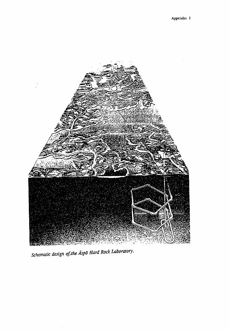
Appendix 1

Schematic design ofshe Äspö Hard Rock Laboratory.

INPUT DATA FILEAppendix 2:1

ASPO.DATA Pri Jun 2 19:25:19 1995

METRIC 19:13 2 JUN 95-- ECLipse data fileRUNSPECMALIHA= NDIVIX NDIVIY NDIVIZ QRDIAL NUMRES QNNC MXAQN MXAQC QPORO QPERM NFSEG

15 5 7 F 1 T 7 0 7 0 F F 0 /= OIL WAT GAS DGAS VOIL API PLY BRI NOTRC NWTRC NGTRC MISC GI SOLV SFT

F T F F F F F F O 1 0 F F F F /= UNIT CONVENTION

' M E T R I C /= NRPVT NPPVT NTPVT NTROCC QROCKC QRCREV QROCKH QVE2D SURFT MDIFF QCOAL

20 20 1 1 F T F F F F F /= NSS NTS DIRK REVK VEOP HYST SCAL SDIR SREV NSEND NTEND 2PT NSMIS NTMIS

20 1 F T F F F F T 2 0 1 F 2 0 1 /= NDRXVD NTEQUL NDPRVD QUIESC QTHPRS QREVTH QMOBIL NTTRVD NSTRVD

20 1 100 F F T F 1 20 /= NTFIP QGRAID QINTRP QTDISP NTFREG QTDISK NRFREG NHFIPR NETRAC

1 F F F 0 F 0 1 0 /= NWMAXZ NCWMAX NGMAXZ NWGMAX MAXLGR MAXCLS MCOARS LSTACK

3 9 0 3 0 0 0 10/= QEXGOP NWFRIC NUPCOL

F 0 3 /= MXMFLO MXMTHP MXMWFR MXMGFR MXMALQ NMMVFT

0 0 0 0 0 0 /= MXSFLO MXSTHP NMSVFT

0 0 0 /= NANAQU NCAMAX NIFTBL NRIFTB NSUMMX

0 70 0 0 3000 /DAY MONTH YEAR

1 ' J A N ' 1990 /= QSOLVE NSTACK QFMTOU QFMTIN QUNOUT QUNINP NGDISK IDYNAM QOPT9? NDMAIN

T 5 6 F F F F 0 0 F 1 /

GRID

DXV10.0000010.0000010.00000

METRIC 11:05 7 MAY 9510.00000 10.00000 10.00000 10.00000 10.00000 10.0000010.00000 10.00000 10.00000 10.00000 10.00000 10.00000

DYV METRIC 1 1 : 0 6 7 MAY 9510.00000 10.00000 10.00000 10.00000 10.00000

/

DZ METRIC 1 1 : 0 7 7 MAY 95

525*10.00

TOPS METRIC 08:55 31 MAY 95.

75*13075*14075*15075*16075*17075*18075*190

Appendix 2:2

ASPO.DATA Fri Jun 2 19:25:19 1995 2

PORO METRIC 1 1 : 4 5 2 1 MAY 9 5

525*0.0221111111111

PERMX METRIC 09:06 31 MAY 95

8.00 8.00 8.00 8.00 8.00 8.00 8.00 8.00 8.00 8.00 8.00 8.00 8.00 8.00 8.00

10.0 10.0 10.0 10.0 10.0 10.0 10.0 10.0 10.0 10.0 10.,0 10.0 10.0 10.0 10.0

2000 2000 2000 2000 2000 2000 2000 2000 2000 2000 2000 2000 2000 2000 2000

10.0 10.0 10.0 10.0 10.0 10.0 10.0 10.0 10.0 10.0 10.0 10.0 10.0 10.0 10.0

8.00 8.00 8.00 8.00 8.00 8.00 8.00 8.00 8.00 8.00 8.00 8.00 8.00 8.00 8.00

8.00 8.00 8.00 8.00 8.00 8.00 8.00 8.00 8.00 8.00 8.00 8.00 8.00 8.00 8.00

10.0 10.0 10.0 10.0 10.0 10.0 10.0 10.0 10.0 10.0 10.0 10.0 10.0 10.0 10.0

2000 2000 2000 2000 2000 2000 2000 2000 2000 2000 2000 2000 2000 2000 2000

10.0 10.0 10.0 10.0 10.0 10.0 10.0 10.0 10.0 10.0 10.0 10.0 10.0 10.0 10.0

8.00 8.00 8.00 8.00 8.00 8.00 8.00 8.00 8.00 8.00 8.00 8.00 8.00 8.00 8.00

8.00 8.00 8.00 8.00 8.00 8.00 8.00 8.00 8.00 8.00 8.00 8.00 8.00 8.00 8.00

10.0 10.0 10.0 10.0 10.0 10.0 10.0 10.0 10.0 10.0 10.0 10.0 10.0 10.0 10.0

2000 2000 2000 2000 2000 2000 2000 2000 2000 2000 2000 2000 2000 2000 2000

10.0 10.0 10.0 10.0 10.0 10.0 10.0 10.0 10.0 10.0 10.0 10.0 10.0 10.0 10.0

8.00 8.00 8.00 8.00 8.00 8.00 8.00 8.00 8.00 8.00 8.00 8.00 8.00 8.00 8.00

8.00 8.00 8.00 8.00 8.00 8.00 8.00 8.00 8.00 8.00 8.00 8.00 8.00 8.00 8.00

10.0 10.0 10.0 10.0 10.0 10.0 10.0 10.0 10.0 10.0 10.0 10.0 10.0 10.0 10.0

2000 2000 2000 2000 2000 2000 2000 2000 2000 2000 2000 2000 2000 2000 2000

10.0 10.0 10.0 10.0 10.0 10.0 10.0 10.0 10.0 10.0 10.0 10.0 10.0 10.0 10.0

8.00 8.00 8.00 8.00 8.00 8.00 8.00 8.00 8.00 8.00 8.00 8.00 8.00 8.00 8.00

8.00 8.00 8.00 8.00 8.00 8.00 8.00 8.00 8.00 8.00 8.00 8.00 8.00 8.00 8.00

10.0 10.0 10.0 10.0 10.0 10.0 10.0 10.0 10.0 10.0 10.0 10.0 10.0 10.0 10.0

2000 2000 2000 2000 2000 2000 2000 2000 2000 2000 2000 2000 2000 2000 2000

10.0 10.0 10.0 10.0 10.0 10.0 10.0 10.0 10.0 10.0 10.0 10.0 10.0 10.0 10.0

8.00 8.00 8.00 8.00 8.00 8.00 8.00 8.00 8.00 8.00 8.00 8.00 8.00 8.00 8.00

8.00 8.00 8.00 8.00 8.00 8.00 8.00 8.00 8.00 8.00 8.00 8.00 8.00 8.00 8.00

Appendix 2:3

ASPO.DATA Fri Jun 2 19:25:19 1995 3

10.0 10.0 10.0 10.0 10.0 10.0 10.0 10.0 10.0 10.0 10.0 10.0 10.0 10.0 10.0

2000 2000 2000 2000 2000 2000 2000 2000 2000 2000 2000 2000 2000 2000 2000

10.0 10.0 10.0 10.0 10.0 10.0 10.0 10.0 10.0 10.0 10.0 10.0 10.0 10.0 10.0

8.00 8.00 8.00 8.00 8.00 8.00 8.00 8.00 8.00 8.00 8.00 8.00 8.00 8.00 8.00

8.00 8.00 8.00 8.00 8.00 8.00 8.00 8.00 8.00 8.00 8.00 8.00 8.00 8.00 8.00

10.0 10.0 10.0 10.0 10.0 10.0 10.0 10.0 10.0 10.0 10.0 10.0 10.0 10.0 10.0

2000 2000 2000 2000 2000 2000 2000 2000 2000 2000 2000 2000 2000 2000 2000

10.0 10.0 10.0 10.0 10.0 10.0 10.0 10.0 10.0 10.0 10.0 10.0 10.0 10.0 10.0

8.00 8.00 8.00 8.00 8.00 8.00 8.00 8.00 8.00 8.00 8.00 8.00 8.00 8.00 8.00

IIIII III 11

PERMY METRIC 09:06 31 MAY 95

8.00 8.00 8.00 8.00 8.00 8.00 8.00 8.00 8.00 8.00 8.00 8.00 8.00 8.00 8.00

10.0 10.0 10.0 10.0 10.0 10.0 10.0 10.0 10.0 10.0 10.0 10.0 10.0 10.0 10.0

2000 2000 2000 2000 2000 2000 2000 2000 2000 2000 2000 2000 2000 2000 2000

10.0 10.0 10.0 10.0 10.0 10.0 10.0 10.0 10.0 10.0 10.0 10.0 10.0 10.0 10.0

8.00 8.00 8.00 8.00 8.00 8.00 8.00 8.00 8.00 8.00 8.00 8.00 8.00 8.00 8.00

8.00 8.00 8.00 8.00 8.00 8.00 8.00 8.00 8.00 8.00 8.00 8.00 8.00 8.00 8.00

10.0 10.0 10.0 10.0 10.0 10.0 10.0 10.0 10.0 10.0 10.0 10.0 10.0 10.0 10.0

2000 2000 2000 2000 2000 2000 2000 2000 2000 2000 2000 2000 2000 2000 2000

10.0 10.0 10.0 10.0 10.0 10.0 10.0 10.0 10.0 10.0 10.0 10.0 10.0 10.0 10.0

8.00 8.00 8.00 8.00 8.00 8.00 8.00 8.00 8.00 8.00 8.00 8.00 8.00 8.00 8.00

8.00 8.00 8.00 8.00 8.00 8.00 8.00 8.00 8.00 8.00 8.00 8.00 8.00 8.00 8.00

10.0 10.0 10.0 10.0 10.0 10.0 10.0 10.0 10.0 10.0 10.0 10.0 10.0 10.0 10.0

2000 2000 2000 2000 2000 2000 2000 2000 2000 2000 2000 2000 2000 2000 2000

10.0 10.0 10-0 10.0 10.0 10.0 10.0 10.0 10.0 10.0 10.0 10.0 10.0 10.0 10.0

8.00 8.00 8.00 8.00 8.00 8.00 8.00 8.00 8.00 8.00 8.00 8.00 8.00 8.00 8.00

8.00 8.00 8.00 8.00 8.00 8.00 8.00 8.00 8.00 8.00 8.00 8.00 8.00 8.00 8.00

10.0 10.0 10.0 10.0 10.0 10.0 10.0 10.0 10.0 10.0 10.0 10.0 10.0 10.0 10.0

2000 2000 2000 2000 2000 2000 2000 2000 2000 2000 2000 2000 2000 2000 2000

Appendix 2:4

ASPO.DATA F r i Jun 2 19:25:19 1995 i

1 0 . 0 1 0 . 0 1 0 . 0 1 0 . 0 1 0 . 0 1 0 . 0 1 0 . 0 1 0 . 0 1 0 . 0 1 0 . 0 1 0 . 0 1 0 . 0 1 0 . 0 1 0 . 0 1 0 . 0

8 . 0 0 8 . 0 0 8 . 0 0 8 . 0 0 8 . 0 0 8 . 0 0 8 . 0 0 8 . 0 0 8 . 0 0 8 . 0 0 8 . 0 0 8 . 0 0 8 . 0 0 8 . 0 0 8 . 0 0

8.00 8.00 8.00 8.00 8.00 8.00 8.00 8.00 8.00 8.00 8.00 8.00 8.00 8.00 8.00

10.0 10.0 10.0 10.0 10.0 10.0 10.0 10.0 10.0 10.0 10.0 10.0 10.0 10.0 10.0

2000 2000 2000 2000 2000 2000 2000 2000 2000 2000 2000 2000 2000 2000 2000

10.0 10.0 10.0 10.0 10.0 10.0 10.0 10.0 10.0 10.0 10.,0 10.0 10.0 10.0 10.0

8.00 8.00 8.00 8.00 8.00 8.00 8.00 8.00 8.00 8.00 8.00 8.00 8.00 8.00 8.00

8.00 8.00 8.00 8.00 8.00 8.00 8.00 8.00 8.00 8.00 8.00 8.00 8.00 8.00 8.00

10.0 10.0 10.0 10.0 10.0 10.0 10.0 10.0 10.0 10.0 10.0 10.0 10.0 10.0 10.0

2000 2000 2000 2000 2000 2000 2000 2000 2000 2000 2000 2000 2000 2000 2000

10.0 10.0 10.0 10.0 10.0 10.0 10.0 10.0 10.0 10.0 10.0 10.0 10.0 10.0 10.0

8.00 8.00 8.00 8.00 8.00 8.00 8.00 8.00 8.00 8.00 8.00 8.00 8.00 8.00 8.00

8.00 8.00 8.00 8.00 8.00 8.00 8.00 8.00 8.00 8.00 8.00 8.00 8.00 8.00 8.00

10.0 10.0 10.0 10.0 10.0 10.0 10.0 10.0 10.0 10.0 10.0 10.0 10.0 10.0 10.0

2000 2000 2000 2000 2000 2000 2000 2000 2000 2000 2000 2000 2000 2000 2000

10.0 10.0 10.0 10.0 10.0 10.0 10.0 10.0 10.0 10.0 10.0 10.0 10.0 10.0 10.0

8.00 8.00 8.00 8.00 8.00 8.00 8.00 8.00 8.00 8.00 8.00 8.00 8.00 8.00 8.00

11II11111111 .

PERMZ METRIC 09:42 31 MAY 95

10.0 10.0 10.0 10.0 10.0 10.0 10.0 10.0 10.0 10.0 10.0 10.0 10.0 10.0 10.0

500. 500. 500. 500. 500. 500. 500. 500. 500. 500. 500. 500. 500. 500. 500.

9000.0 9000.0 9000.0 9000.0 9000.0 9000.0 9000.0 9000.0 9000.0 9000.0 9000.09000.0 9000.0 9000.0 9000.0500. 500. 500. 500. 500. 500. 500. 500. 500. 500. 500. 500. 500. 500. 500.

10.0 10.0 10.0 10.0 10.0 10.0 10.0 10.0 10.0 10.0 10.0 10.0 10.0 10.0 10.0

10.0 10.0 10.0 10.0 10.0 10.0 10.0 10.0 10.0 10.0 10.0 10.0 10.0 10.0 10.0

500. 500. 500. 500. 500. 500. 500. 500. 500. 500. 500. 500. 500. 500. 500.

9000.0 9000.0 9000.0 9000.0 9000.0 9000.0 9000.0 9000.0 9000.0 9000.0 9000.09000.0 9000.0 9000.0 9000.0

500. 500. 500. 500. 500. 500. 500. 500. 500. 500. 500. 500. 500. 500. 500.

10.0 10.0 10.0 10.0 10.0 10.0 10.0 10.0 10.0 10.0 10.0 10.0 10.0 10.0 10.0

Appendix 2:5

ASPO.DATA Pri Jun 2 19:25:19 1995 5

10.0 10.0 10 .0 10.0 10.0 10 .0 10.0 10.0 10.0 10.0 10 .0 10 .0 10.0 10.0 10 .0

500. 500. 500. 500. 500. 500. 500. 500. 500. 500. 500. 500. 500. 500. 500.

9000.0 9000.0 9000.0 9000.0 9000.0 9000.0 9000.0 9000.0 9000.0 9000.0 9000.09000.0 9000.0 9000.0 9000.0

500. 500. 500. 500. 500. 500. 500. 500. 500. 500. 500. 500. 500. 500. 500.

10.0 10.0 10.0 10.0 10.0 10.0 10.0 10.0 10.0 10.0 10.0 10.0 10.0 10.0 10.0

10.0 10.0 10.0 10.0 10.0 10.0 10.0 10.0 10.0 10.0 10.0 10.0 10.0 10.0 10.0

500. 500. 500. 500. 500. 500. 500. 500. 500. 500. 500. 500. 500. 500. 500.

9000.0 9000.0 9000.0 9000.0 9000.0 9000.0 9000.0 9000.0 9000.0 9000.0 9000.0

9000.0 9000.0 9000.0 9000.0500. 500. 500. 500. 500. 500. 500. 500. 500. 500. 500. 500. 500. 500. 500.

10.0 10.0 10.0 10.0 10.0 10.0 10.0 10.0 10.0 10.0 10.0 10.0 10.0 10.0 10.0

10.0 10.0 10.0 10.0 10.0 10.0 10.0 10.0 10.0 10.0 10.0 10.0 10.0 10.0 10.0

500. 500. 500. 500. 500. 500. 500. 500. 500. 500. 500. 500. 500. 500. 500.

9000.0 9000.0 9000.0 9000.0 9000.0 9000.0 9000.0 9000.0 9000.0 9000.0 9000.0

9000.0 9000.0 9000.0 9000.0500. 500. 500. 500. 500. 500. 500. 500. 500. 500. 500. 500. 500. 500. 500.

10.0 10.0 10.0 10.0 10.0 10.0 10.0 10.0 10.0 10.0 10.0 10.0 10.0 10.0 10.0

10.0 10.0 10.0 10.0 10.0 10.0 10.0 10.0 10.0 10.0 10.0 10.0 10.0 10.0 10.0

500. 500. 500. 500. 500. 500. 500. 500. 500. 500. 500. 500. 500. 500. 500.

9000.0 9000.0 9000.0 9000.0 9000.0 9000.0 9000.0 9000.0 9000.0 9000.0 9000.09000.0 9000.0 9000.0 9000.0

500. 500. 500. 500. 500. 500. 500. 500. 500. 500. 500. 500. 500. 500. 500.

10.0 10.0 10.0 10.0 10.0 10.0 10.0 10.0 10.0 10.0 10.0 10.0 10.0 10.0 10.0

10.0 10.0 10.0 10.0 10.0 10.0 10.0 10.0 10.0 10.0 10.0 10.0 10.0 10.0 10.0

500. 500. 500. 500. 500. 500. 500. 500. 500. 500. 500. 500. 500. 500. 500.

9000.0 9000.0 9000.0 9000.0 9000.0 9000.0 9000.0 9000.0 9000.0 9000.0 9000.09000.0 9000.0 9000.0 9000.0

500. 500. 500. 500. 500. 500. 500. 500. 500. 500. 500. 500. 500. 500. 500.

10.0 10.0 10.0 10.0 10.0 10.0 10.0 10.0 10.0 10.0 10.0 10.0 10.0 10.0 10.0

AQUNUM METRIC 1 8 : 4 7 2 JUN 951 1 1 1 100.000000 1000.00, , 2000.0, , /2 1 2 1 100.000000 1000.00, , 2000.0, , /3 1 3 1 100.000000 1000.00, , 2000.0, , /4 1 4 1 100.000000 1000.00, , 2000.0, , /5 1 5 1 100.000000 1000.00, , 2000.0, , /6 1 1 2 100.000000 1000.00, , 2000.0, , /7 1 2 2 100.000000 1000.00, , 2000.0, , /

Appendix

ASPO

391011121314151617181920212223242526272829303132333435363738394041424344454647484950515253545556575859606162636465666768S970

.DATA

11111111111111111111111111111515151515151515151515151515151515151515151515151515151515151515151515

345123451234512345123451234512345123451234512345123451234512345

22233333444445555566ggg7777711111222223333344444555556666677777

Fri Jun 2 19

100.000000100.000000100.000000100.000000100.000000100.000000100.000000100.000000100.000000100.000000100.000000100.000000100.000000100.000000100.000000100.000000100.000000100.000000100.000000100.000000100.000000100.000000100.000000100.000000100.000000100.000000100.000000100.000000100.000000100.000000100.000000100.000000100.000000100.000000100.000000100.000000100.000000100.000000100.000000100.000000100.000000100.000000100.000000100.000000100.000000100.000000100.000000100.000000100.000000100.000000100.000000100.000000100.000000100.000000100.000000100.000000100.000000100.000000100.000000100.000000100.000000100.000000100.000000

:25:19 1995

1000.00,1000.00,1000.00.1000.00,1000.00,1000.00,1000.00,1000.00,1000.00,1000.00,1000.00,1000.00,1000.00,1000.00,1000.00,1000.00,1000.00,1000.00,1000.00,1000.00,1000.00,1000.00,1000.00,1000.00,1000.00,1000.00,1000.00,1000.00,1000.00,1000.00,1000.00,1000.00,1000.00,1000.00,1000.00,1000.00,1000.00,1000.00,1000.00,1000.00,1000.00,1000.00,1000.00,1000.00,1000.00,1000.00,1000.00,1000.00,1000.00,1000.00,1000.00,1000.00,1000.00,1000.00,1000.00,1000.00,1000.00,1000.00,1000.00,1000.00,1000.00,1000.00,1000.00,

6

, 2000.0,, 2000.0,, 2000.0,, 2000.0,, 2000.0,, 2000.0,, 2000.0,, 2000.0,, 2000.0,, 2000.0,, 2000.0,, 2000.0,, 2000.0,, 2000.0,, 2000.0,, 2000.0,•, 2000.0,, 2000.0,, 2000.0,, 2000.0,, 2000.0,, 2000.0,, 2000.0,, 2000.0,, 2000.0,, 2000.0,, 2000.0,, 2000.0,, 2000.0,, 2000.0,, 2000.0,, 2000.0,, 2000.0,, 2000.0,, 2000.0,, 2000.0,, 2000.0,, 2000.0,, 2000.0,, 2000.0,, 2000.0,, 2000.0,, 2000.0,, 2000.0,, 2000.0,, 2000.0,, 2000.0,, 2000.0,, 2000.0,, 2000.0,, 2000.0,, 2000.0,, 2000.0,, 2000.0,, 2000.0,, 2000.0,, 2000.0,, 2000.0,, 2000.0,, 2000.0,, 2000.0,, 2000.0,, 2000.0,

///////////////////////////////////////////////////////////

.//,1

Appendix 2:7

ASPO.DATA

AQUCON1234567S910111213141516171819202122232425262728293031323334353637383940414243444546474849505152535455565758596061626364

222222222222222222222222222222222221414141414141414141414141414141414141414141414141414141414

222222222222222222222222222222222221414141414141414141414141414141414141414141414141414141414

Pri

1234512345123451234512345123451234512345123451234512345123451234

Jun

1234512345123451234512345123451234512345123451234512345123451234

2 19

1111122222333334444455555666667777711111222223333344444555556666

:25:

11111222223333344444555556666677777111112222233333444445555566o5

19 1995 7

MI•I-' 1.000000'I-' 1.000000'I-' 1.000000'!-• 1.000000'I-' 1.000000'I-' 1.000000'I-' 1.000000'I-' 1.000000'I-' 1.000000'I-' 1.000000'I-' 1.000000'I-' 1.000000'I-' 1.000000'!-' 1.000000'I-' 1.000000'I-' 1.000000'I-' 1.000000•I-1 1.000000'I-' 1.000000'I-' 1.000000'I-' 1.000000'I-' 1.000000•I-' 1.000000'I-' 1.000000•I-' 1.000000'I-' 1.000000•I-' 1.000000'I-' 1.000000'I-' 1.000000'I-' 1.000000'I-' 1.000000'I-' 1.000000'I-' 1.000000'I-' 1.000000'I-' 1.000000'I+' 1.000000'I+' 1.000000'I+' 1.000000'I+' 1.000000'3>' 1.000000'I+' 1.000000'I+' 1.000000'I+' 1.000000'I+' 1.000000'I+' 1.000000'I+' 1.000000'I+' 1.000000'I+' 1.000000'I+' 1.000000'I+' 1.000000'I+' 1.000000'1+' 1.000000'I+' 1.000000'I+' 1.000000'I+' 1.000000'I+' 1.000000'I+' 1.000000'I+' 1.000000'I+' 1.000000'I+' 1.000000'I+' 1.000000'I+' 1.000000' I *' 1."'- 0 0 0 0':••' :. K O C O O

2T:1111111111111111111111111111111111111111111111111111111111111111

METRIC 1 9 : 1 1 2 JUN 95

Appendix 2:8

ASPO.DATA Fri Jun 2 19:25:: 1995

656667636970

14 1414 1414 1414 1414 1414 14

512345

677777

677777

'I+''I+''I+''I+1

'I+'

1.0000001.0000001.0000001.0000001.0000001.000000

111111

OLDTRAN

INIT

RPTGRID0 00 00 0

PROPS

METRIC 15:20 23 MAY 95O i l 1 0 0 0 1 0 1 0 0 00 0 0 0 0 0 0 0 0 0 0 0 00 0 0 0 0 0 0 0 0 0 0 /

DENSITY 1 TABLES 20 P NODES800.000 1000.00 0.50000 /

PVTW 1 TABLES 20 P NODES0.0000000 1.00000 .5100E-04

ROCK0.00000

TRACER'RWT',

1 TABLES 20 P NODES0.0010000 /

'WAT'

20 R NODES METRIC 20:31 5 MAY 95

20 R NODES METRIC 11:48 21 MAY 950.30000 0.00E+OO /

20 R NODES METRIC 16:00 15 MAY 95

METRIC 17:54 2 MAY 95

RPTPROPS0 00 0

SOLUTION

PRESSURE

00

00

10

00

10

10

00

METRIC 15:21 23 MAY 95'

METRIC 16:12 21 MAY"95" -,

75*2075*2075*2075*2075*2075*2075*20 /

TBLKFRWT METRIC 19:08 20 MAY 95

RPTSOL10

00

10

75 *075*03030303075

*0*0*0*0*0

00

00

13*013*013*013*0

00

00

1*11*.1*.1*./

00

.0000000

00

1*01*01*01*0

00

30*030*030*030*0

M00

METRIC 15:21 23 MAY 950 0 0 00 0 0 0

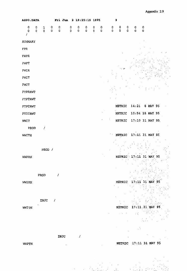
Appendix 2:9

ASPO.DATA Pri Jun 2 19:25:19 1995

00

0

o

SUMMARY

FPR

FWPR

FWPT

FWIR

FWIT

FWCT

FTPRRWT

FTPTRWT

FTPCRWT

FTICRWT

WWCT

PROD

WWCTH

10

00

00

00

00

00

00

0

ooo

oo

oo

oo



METRIC 17:10 31 MAY 95.

METRIC 17:11 31 MAY 9E

WWPRH

PROD /


WWIRH

PROD


WWITH

INJC

METRIC 17:11.31 MAY 95,

WWPTH

INJC


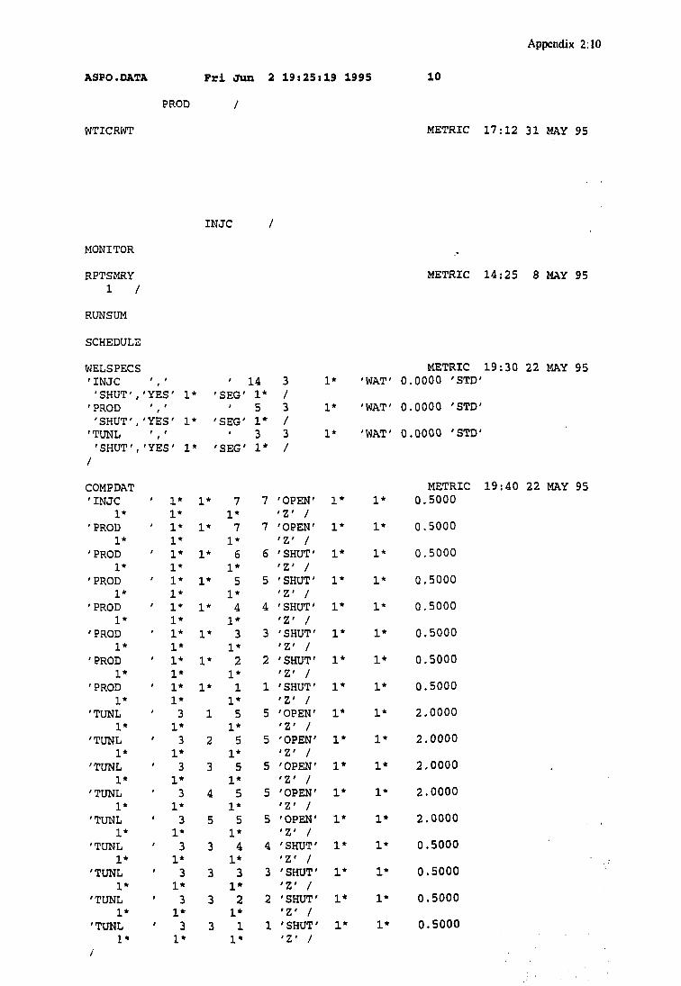
ASPO.DATA F r i Jun 2 19:25:19 1995

PROD /

WTICRWT

Appendix 2:10

10


INJC /

MONITOR

RPTSMRY1 /

RUNSUM

SCHEDULE

WELSPECS'INJC ', ' ' 14 3'SHUT','YES' 1* 'SEG' 1* /'PROD ', ' '53'SHUT','YES' 1* 'SEG' 1* /'TUNL ',' '33'SHUT','YES' 1* 'SEG' 1* /


METRIC 19:30 22 MAY 951* 'WAT' 0.0000 'STD'

1* 'WAT' 0.0000 'STD'

1* 'WAT' 0.0000 'STD'

COMPDAT'INJC

1*'PROD

1*'PROD

1*'PROD

1*'PROD

1*'PROD

1*'PROD

1*'PROD

1*'TUNL

1*'TUNL

1*'TUNL

1*'TUNL

1*'TUNL

1*'TUNL

1*'TUNL

1*'TUNL

1*'TUNL

1*

' 1*1*

' 1*1*

' 1*1*

' 1*1*

' 1*1*

' 1*1*

' 1*1*

' 1*1*31*31*31*31*31*31*31*31*31*

1*

1*

1*

1*

1*

1*

1*

1*

1

2

3

4

5

3

3

3

3

71*71*61*51*41*31*21*11*51*51*51*51*51*41*31*21*11*

7

7

6

5

4

3

2

1

5

5

5

5

5

4

3

2

1

'OPEN''Z' /'OPEN''Z' /'SHUT''Z' /'SHUT''Z' /'SHUT''Z' /'SHUT''Z' /'SHUT''Z' /'SHUT''Z' /'OPEN''Z' /'OPEN''Z' /'OPEN''Z' /'OPEN''Z' /'OPEN''Z' /'SHUT''Z' /'SHUT''Z' /'SHUT''Z' /'SHUT''Z' /

1*

1*

1*

1*

1*

1*

1*

1*

1*

1*

1*

1*

1*

1*

1*

1*

1*

1*

1*

1*

1*

1*

1*

1*

1*

1*

1*

1*

1*

1*

1*

1*

1*

1*

0

0

0

0

0

0

0

0

2

2

2

2

2

0

0

0

0

METRIC 19:40 22 MAY 95.5000

.5000

.5000

.5000

.5000

.5000

.5000

.5000

.0000

.0000

.0000

.0000

.0000

.5000

.5000

.5000

.5000

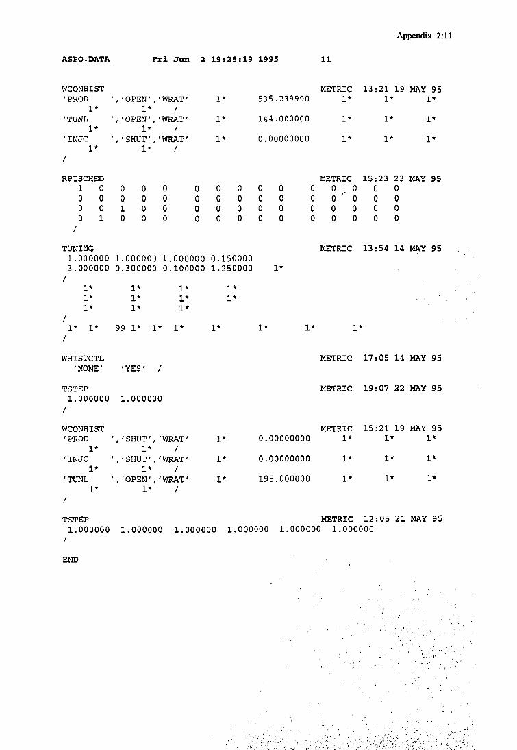
Appendix 2:11

AS PO.DATA Fri Jun 2 19:25:19 1995 11

WCONHIST'PROD ','OPEN','WRAT' 1*

1* I" /'TUNL ','OPEN','WRAT' 1*

1* 1* /'INJC ','SHUT','WRAT' 1*

1* 1* /

METRIC 13:21 19 MAY 95535.239990 1* 1* 1*

144.000000

0.00000000

I1

V V

1*

1*

RPTSCHED1000

0001

0010

0000

0000

0000

0000

0000

0000

0000

METRIC 15:23 23 MAY 950 0 . 0 0 00 0 " 0 0 00 0 0 0 00 0 0 0 0

TUNING1.000000 1.000000 1.000000 0.1500003.000000 0.300000 0.100000 1.250000 1*

1*1*1*

1*1*1*

99 1* V

1*1*1*

1*1*


WHISTCTL'NONE' 'YES'

TSTEP1.000000 1.000000



WCONHIST'PROD ','SHUT','WRAT'

1* 1* /'INJC ','SHUT','WRAT'

1* 1* /'TUNL ','OPEN','WRAT'

1* 1* //

TSTEP

1*

1*

1*

METRIC 15:21 19 MAY 950.00000000 1* 1* 1*

0.00000000

195.000000

1*

1*

1*

1*

1*

1*

METRIC 12:05 21 MAY 951.000000 1.000000 1.000000 1.000000 1.000000 1.000000

END

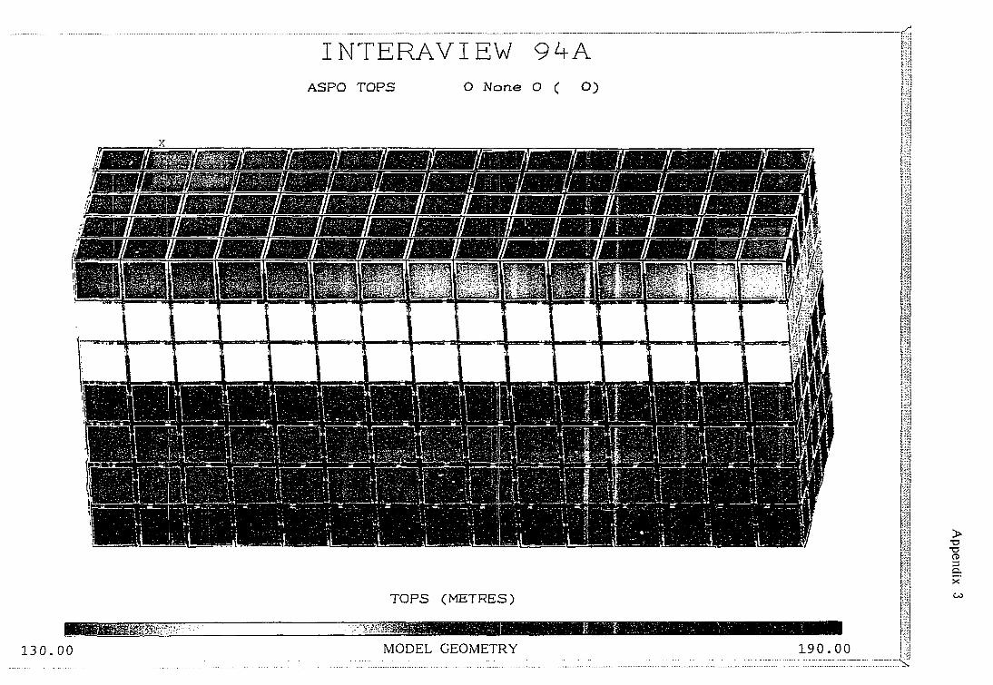
INTERAVIEW 94AASPO TOPS O None O ( O)

•o•a

c

TOPS (METRES)

130.00 MODEL GEOMETRY 190.00

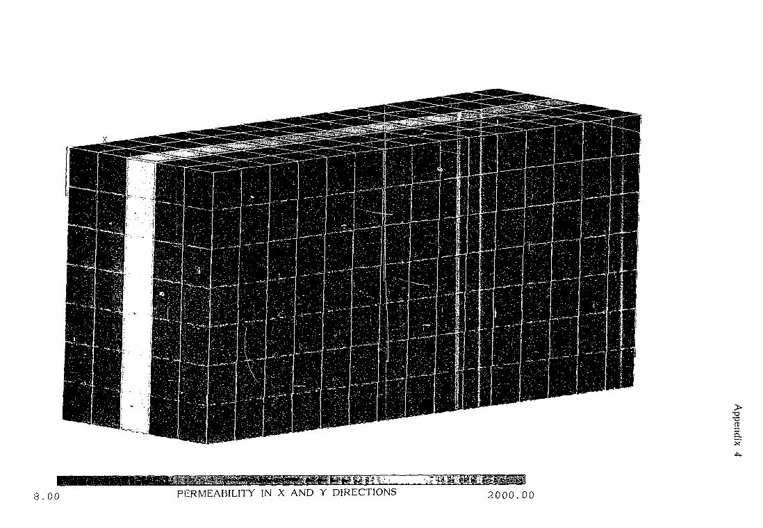
>T3•OCO3

3 .0 0 PERMEABILITY IN X AND Y DIRECTIONS 2000 .00

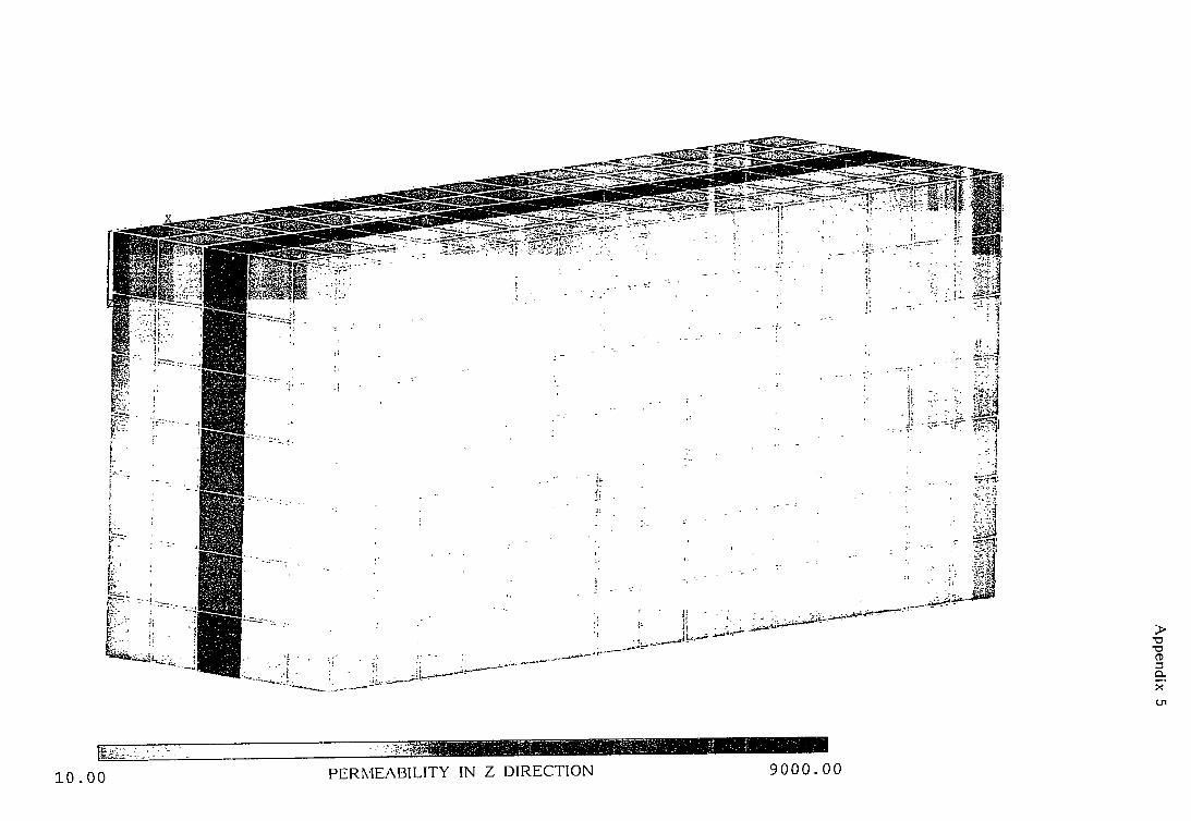
CD

Q.

1 0 . 0 0 PERMEABILITY IN Z DIRECTION 9 0 0 0 . 0 0

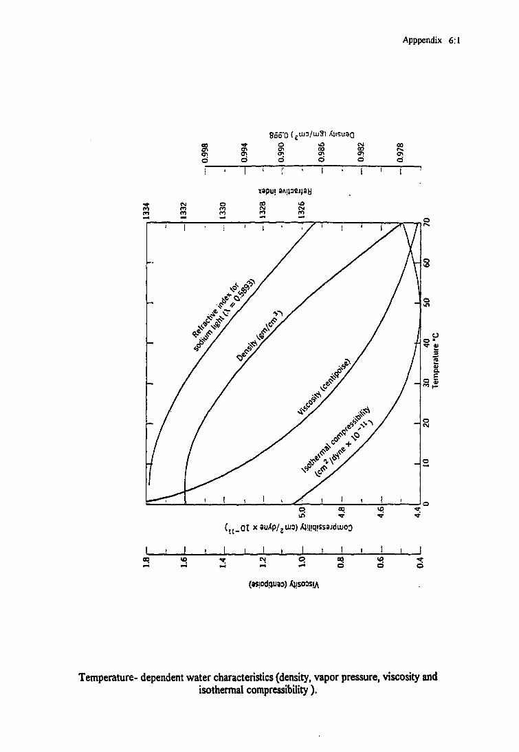
Apppendix 6:1

d

8560 'o vO

ena; 00

o di r i i

xspui aAi

PImorom

00

m PO

Temperature- dependent water characteristics (density, vapor pressure, viscosity andisothermal compressibility).

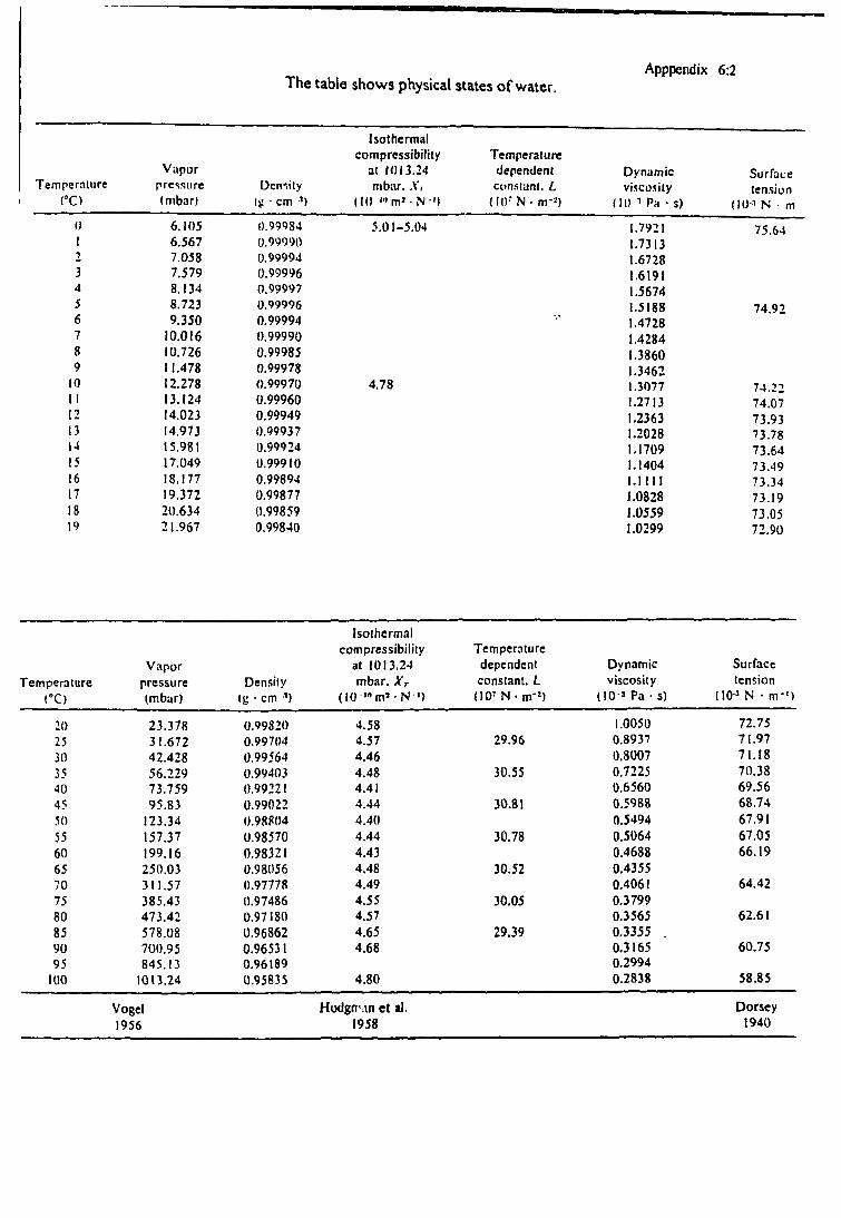
TemperatureCO

0

123456789

101!1213141516171819

Vaporpressure(mbar)

6.1056.5677.0587.5798.1348.7239.350

10.01610.72611.47812.27813.12414.02314.97315.98117.04918.17719.37220.63421.967

The table

DensityIg • cm -1)

0.999840.999900.999940.999960.999970.999960.999940.999900.999850.999780.999700.999600.999490.999370.999240.999100.998940.998770.998590.99840

shows physical states of water.

Isothermalcompressibility Temperature

at 1013.24 dependentmbar. X, constant. L

(10 ' » m ' - N - ' l ( I O : N - m-0

5.01-5.04

4.78

Apppendix

Dynamicviscosity

(II) ' Pa -s)

1.79211.73131.67281.61911.56741.51881.47281.42841.3860.3462.3077.2713.2363.2028.1709.1404.1111.0828.0559.0299

6:2

Surfacetension

(IO-i N • m

75.64

74.92

74.2274.0773.9373.7873.6473.4973.3473.1973.0572.90

Temperature<°C)

20253035404550556065707580859095

100

Vaporpressure(mbar)

23.37831.67242.42856.22973.75995.83

123.34157.37199.16250.03311.57385.43473.42578.08700.95845.13

1013.24

Vogel1956

Density(g • cm ••*)

0.998200.997040.995640.994030.992210.990220.988040.985700.983210.980560.977780.974860.971800.968620.965310.961890.95835

Isothermalcompressibility

at 1013,24mbar. XT

(10 " m ' - N ')

4.584.574.464.484.414.444.404.444.434.484.494.554.574.654.68

4.80

Hodgrr.in et al.1958

Temperaturedependentconstant. LU0TN-m-3)

29.96

30.55

30.81

30.78

30.52

30.05

29.39

Dynamicviscosity

(I0-3 Pa • s)

1.00500.89370.80070.72250.65600.59880.54940.50640.46880.43550.40610.37990.35650.3355 .0.31650.29940.2838

Surfacetension

(10 J N • m " )

72.7571.9771.1870.3869.5668.7467.9167.0566.19

64.42

62.61

60.75

58.85

Dorsey1940

GROUNDWATER MODELLING OF ÄSPÖ USING THE ...

Documents

Transcript of GROUNDWATER MODELLING OF ÄSPÖ USING THE ...