Seediscussions,stats,andauthorprofilesforthispublicationat:https://www.researchgate.net/publication/223447625

ModellingdeforestationusingGISandartificialneuralnetworks

ArticleinEnvironmentalModellingandSoftware·May2004

DOI:10.1016/S1364-8152(03)00161-0·Source:DBLP

CITATIONS

113

READS

539

4authors,including:

Someoftheauthorsofthispublicationarealsoworkingontheserelatedprojects:

ValoracióndelGeoptrimonioyGeoparquesViewproject

"Prospecciónterritorialanteescenariosdecambioclimáticoencuencasdealtavulnerabilidad:bases

paraelmanejodeinformaciónylaintegracióninter-sectorial"Viewproject

JeanFrançoisMas

UniversidadNacionalAutónomadeMéxico

157PUBLICATIONS2,889CITATIONS

SEEPROFILE

JoseLuisPalacio

UniversidadNacionalAutónomadeMéxico

81PUBLICATIONS820CITATIONS

SEEPROFILE

AtahualpaSosa-Lopez

UniversidadAutónomadeCampeche

23PUBLICATIONS313CITATIONS

SEEPROFILE

AllcontentfollowingthispagewasuploadedbyJoseLuisPalacioon15May2014.

Theuserhasrequestedenhancementofthedownloadedfile.Allin-textreferencesunderlinedinblueareaddedtotheoriginaldocument

andarelinkedtopublicationsonResearchGate,lettingyouaccessandreadthemimmediately.

Environmental Modelling & Software 19 (2004) 461–471www.elsevier.com/locate/envsoft

Modelling deforestation using GIS and artificial neural networks

J.F. Masa,∗, H. Puigb, J.L. Palacioa, A. Sosa-Lo´pezc

a Instituto de Geografıa, Universidad Nacional Autonoma de Mexico (UNAM), Sede Morelia, Aquiles Serdan 382, Colonia Centro,58000 Morelia, Michoacan, Mexico

b Laboratoire d’Ecologie Terrestre, UMR 5552 (CNRS/UPS) 13, Av. du Colonel Roche, B.P. 4072, 31029 Toulouse Cedex 4, Francec Centro de Ecologıa, Pesquerıa y Oceanografıa del Golfo de Mexico (EPOMEX), Universidad Autonoma de Campeche A.P. 520,

24030 Campeche, Camp, Mexico

Received 29 April 2002; received in revised form 26 February 2003; accepted 10 July 2003

Abstract

This study aims to predict the spatial distribution of tropical deforestation. Landsat images dated 1974, 1986 and 1991 wereclassified in order to generate digital deforestation maps which locate deforestation and forest persistence areas. The deforestationmaps were overlaid with various spatial variables such as the proximity to roads and to settlements, forest fragmentation, elevation,slope and soil type to determine the relationship between deforestation and these explanatory variables. A multi-layer perceptronwas trained in order to estimate the propensity to deforestation as a function of the explanatory variables and was used to developdeforestation risk assessment maps. The comparison of risk assessment map and actual deforestation indicates that the model wasable to classify correctly 69% of the grid cells, for two categories: forest persistence versus deforestation. Artificial neural networksapproach was found to have a great potential to predict land cover changes because it permits to develop complex, non-linear models. 2003 Elsevier Ltd. All rights reserved.

Keywords: Deforestation; Land use/land cover change; Spatial modelling; Artificial neural networks; Geographic information system

1. Introduction

Tropical deforestation, as an important factor in globalchange, is a topic that has received considerable atten-tion recently. It has been shown to have a negativeinfluence on regional hydrology, large-scale and long-term climate systems, global biogeochemical cycles andbiodiversity lost (Fontan, 1994; IGBP, 1993; IPCC,1996; Puig, 2000). Despite its importance, accurate stat-istics on deforestation rates are not available in mostcountries (Grainger, 1993). In Mexico, various authorsreported deforestation rates that range between 0.3% and5% by year (Cortina Villar et al., 1999; Dı´az Gallegoset al., 2001; Bocco et al., 2001; Turner et al., 2001; Vel-azquez et al., in press). A recent study (Mas et al., 2002;Velazquez et al., 2002) estimates the nation-wide rate ofdeforestation in about 0.3% and 0.8% by year for tem-plate and tropical forests, respectively, which represents

∗ Corresponding author.E-mail address: jfmas@igiris.igeograf.unam.mx (J.F. Mas).

1364-8152/$ - see front matter 2003 Elsevier Ltd. All rights reserved.doi:10.1016/S1364-8152(03)00161-0

a total loss of 84,000 km2 of forest cover between 1976and 2000. The main agents driving deforestation are wellknown, even though it is difficult to assess their relativecontribution to deforestation and there is not a clearunderstanding on how these factors interact. The simul-ation of land use/cover changes is important for a varietyof management and planning issues as well as for aca-demic research. In the case of deforestation, the develop-ment of models is motivated by several potential bene-fits: (1) to provide a better understanding on how drivingfactors govern deforestation, (2) to generate future scen-arios of deforestation rates, (3) to predict the location offorest clearing and, (4) to support the design of policyresponses to deforestation (Lambin, 1994).

This study aims at developing a simple spatial modelthat is able to predict the location of deforestation usingan artificial neural networks (ANNs) approach.

462 J.F. Mas et al. / Environmental Modelling & Software 19 (2004) 461–471

2. Background

2.1. Land use change models

The projection of land use changes can be performedusing two main categories of models (Lambin, 1997;Stephenne and Lambin, 2001): (1) empirical modelsbased on an extrapolation of the patterns of changeobserved over the recent past, with a limited represen-tation of the driving forces of these changes, and (2)simulation models based on the thorough understandingof the processes of change. The spatial prediction of landuse/cover changes can be obtained by models whichbelong to the first category. Several studies have achi-eved a good projection of likely patterns of landuse/cover change, based on multivariate models rep-resenting the interactions between environmental vari-ables that are controlling the changes. Such spatial mod-els attempt to identify explicitly the proximate causes ofland use/cover change using statistical approaches suchas regression or weight of evidence (Soares-Filho et al.,2002; Schneider and Pontius, 2001; Almeida et al.,2003). They are based upon the assumption that therelationships between the changes and the proximatecauses of these changes remain the same over time and,therefore, can only provide short-range projections (5–10 years at most) due to the dynamic character of landuse/cover change processes.

Many challenges must be faced when attempting todevelop models of land use/cover change processes. Thesite and magnitude of land-use changes are the resultsof human decisions. The main difficulty is the highdegree of complication, the large number of conditions,and the complexity of the interactions between humanand environmental factors (Lambin, 1994). For example,Sader and Joyce (1988) examined forest area changeassociated with factors such as slope and transportationnetworks for Costa Rica. He found a strong relationshipbetween forest clearing and proximity to road. Heobserved also that forest clearing on shallow slopebefore 1961 was low because the 0–5% slopes of theAtlantic low land were inaccessible. The increased clear-ing on shallow slopes occurred in an area previously lessaccessible and recently opened to development by theconstruction of a highway. This very simple exampleshows that forest clearing is not the result of the sum ofthe effects of each factor in an independent form butrather the combination of them. Taking into accountenvironmental, socio-economic and cultural variablesaspects of deforestation processes, relationships betweenthe variables may be very complex. Statistical method,such as logistic regression, may have some limitationswhen variables interact on a complex way. They areinvalid when spatial variables correlate with each otherand have difficulties in handling poor and noisy data (Liand Yeh, 2002). Because ANNs are able to directly take

into account any non-linear complex relationshipbetween the explicative variables and deforestation, bet-ter results can be expected from this approach. A fewland use/cover change model based upon ANNs andfocused on simulating urban growth have been recentlyreported in the literature (Li and Yeh, 2002; Pijanowskiet al., 2002). However there is no model using ANNsaimed at predicting tropical deforestation.

2.2. Artificial neural networks

ANNs are non-linear mapping structures based on thefunction of the human brain. Advantages of the ANNapproach include ability to handle non-linear functions,to perform model-free function estimation, to learn fromdata relationships that are not otherwise known and, togeneralize to unseen situations. ANNs have been shownto be universal and highly flexible function approxima-tors for any data. Therefore, ANNs make powerful toolsfor models, especially when the underlying data relation-ships are unknown (Lek et al., 1996; Lek and Guegan,1999). In the last decade, ANNs have seen an explosionof interest and have been successfully applied across alarge range of domains such as image recognition, medi-cine, molecular biology and, more recently, ecologicaland environmental sciences (Lek and Guegan, 1999;Maier and Dandy, 2000). Some recent utilizations ofANNs in environmental sciences are models predictingspecies distribution, abundance or diversity as a functionof environmental variables (Lek-Ang et al., 1999; Manelet al., 1999), rice crop damage by flamingos (Tourenq etal., 1999), streamflow and flash floods (Kim and Barros,2001), air quality parameters (Abdul-Wahab and Al-Ala-wib, 2002; Chelani et al., 2002) and ecosystem charac-teristics from remotely sensed data (Jensen et al., 1999;Paruelo and Tomasel, 1997).

The multi-layer feed-forward neural network or multi-layer perceptron (MLP), is one of the most popular ANNarchitecture in use today (Bishop, 1995; Atkinson andTatnall, 1997; Lek and Guegan, 1999). The MLP isbased on the supervised procedure, i.e. the network con-structs a model based on examples of data with knownoutputs. The training is done solely from the examplespresented, which are together assumed to implicitly con-tain the information necessary to establish the relation.A MLP is a powerful system, often capable of modellingcomplex relationships between variables. It allows pre-diction of an output object for a given input object or aset of input objects.

The architecture of the MLP is a layered feed-forwardneural network, in which the non-linear elements(neurons) are arranged in successive layers, and theinformation flows unidirectionally, from the input layerto the output layer, through the hidden layer(s): whenthe network is executed, the input variable values areplaced in the input units, and then the hidden and output

463J.F. Mas et al. / Environmental Modelling & Software 19 (2004) 461–471

layer units are progressively executed. Each of them cal-culates its activation value by taking the weighted sumof the outputs of the units in the preceding layer. Theactivation value is passed through the activation functionto produce the outputs of the neuron. When the entirenetwork has been executed, the outputs of the outputlayer act as the output of the entire network (Fig. 1).

The learning procedure is based on a relatively simpleconcept: if the network gives the wrong answer, then theweights are corrected so the error is lessened so futureresponses of the network are more likely to be correct.The best-known example of a neural network-trainingalgorithm is backpropagation. Modern second-orderalgorithms such as Levenberg–Marquadt are faster. Lev-enberg–Marquardt is an advanced non-linear optimiz-ation algorithm. However, its use is restricted to small,single output networks using sum-squared error function(Bishop, 1995).

As the network is trained to minimize the error on thetraining set, a major issue is over learning or over fitting.A network with more weights models a more complexfunction, and is therefore prone to over-fitting (Bishop,1995; Foody and Arora, 1997). In order to avoid overlearning cross-verification is used: some of the trainingcases (verification set) are not actually used for trainingbut to keep an independent check on the progress oftraining. As training progresses, the training error nat-urally drops. If the verification error stops dropping, orstarts to rise, this indicates that the network is startingto over fit the data, and training should cease.

In a classification problem, an output unit’s task is tooutput a strong signal if a case belongs to the class, anda weak signal if it does not. The activation value maybe also considered as a fuzzy membership (Civco, 1993;Foody, 1995), which can be perceived as a measure ofcertainty to belonging at the class. When the ANNs areused to model deforestation as a function of explanatoryvariables, these activation values express the propensity(activation values cannot be properly considered asprobabilities) of deforestation.

Fig. 1. Schematic illustration of a three-layered perceptron, with oneinput layer, one hidden layer and one output layer. In this exampleX1, X2, …, X6 are six input (explanatory) variables (e.g. factors ofdeforestation); Y1 and Y2 are two output variables (e.g. deforestationand regrowth).

3. Study area

The study area is situated in the State of Campeche,south east of Mexico between 18° 00� and 18° 55� Northand 90° 55� and 92° 06� West (Fig. 2) and covers about12,400 km2. Soils are dominated by gleysol; there arealso solonchak and rendzina soils. The study area con-sists of extensive areas of savannah and a mosaic ofmangroves, pastures and remnant tropical forests. Alarge proportion of the land surrounding the Lagoon ofTerminos has been deforested. Major causes of defores-tation are government-directed colonization schemes,cattle ranching and, during the 1980s, rice farming(Isaac-Marquez, 1993; Mas and Puig, 2001). The maintown in the study area is Ciudad del Carmen (84,000inhabitants). There are also several towns and hundredsof villages in the study area and its surrounding. In 1994,an important part of the area has been declared as nat-ure reserve.

4. Material and methods

Two Landsat MSS images (path 21, row 47) dated15/2/1974 and 15/1/1986 and a Landsat TM image dated3/4/1991 were obtained. The Landsat data were geo-metrically corrected and registered to a common UTMprojection with an RMS error of less than 1.0 pixel.Digital maps of soils, road networks and human settle-ments were produced by manual digitisation of theNational Institute of Geography, Statistics and Informat-ics (INEGI) 1:250,000-scale maps and the satelliteimages data. A digital elevation model generated from10-m contour lines was used to create a slope map.

Fig. 2. Localization of the study area.

464 J.F. Mas et al. / Environmental Modelling & Software 19 (2004) 461–471

As shown in Fig. 3, the model discussed in this paperfollows five sequential steps: (1) elaboration of maps ofdeforestation obtained by overlaying maps of forestcover from more than one point in time, (2) quantifi-cation of the relationships between deforestation andproximate causes and selection of the “best” explanatoryvariables, (3) calibration of the model (training of theANN), (4) simulation (elaboration of a map of propen-sity to deforestation which predicts deforestation for thefollowing period) and (5) assessment of the model per-formance (comparison between actual and predicteddeforestation).

4.1. Deforestation monitoring

In a previous study several techniques of changedetection, such as image differencing, selective principalcomponents analysis, direct multidate unsupervisedclassification and post-classification image comparison,have been tested in order to determinate the optimal pro-cedure to assess deforestation in this area. Post-classi-fication comparison was found to be the more accuratetechnique because it was less sensitive to radiometricvariations due to the difference in soil moisture and veg-etation phenology between scenes from different dates(Mas, 1999). Therefore, images were classified indepen-dently using the maximum likelihood algorithm into thefollowing land cover classes: “undisturbed” tropical for-est, secondary tropical forest, mangroves and non-forestvegetation. Classification accuracy was evaluated by cal-culating global accuracy and Kappa coefficient using an

Fig. 3. Flowchart of the neural-network based model for simulating deforestation.

independent sample of 106 reference points obtainedfrom 1:50,000-scale aerial photographs interpretation.Areas of forest were calculated for the three dates andannual rates of forest clearing were estimated. Classifiedimages were simplified by grouping tropical forest (bothundisturbed and secondary) into a single “ forest” classand all other land cover classes in another “no-forest”class. Thus, the final images, after completing this pro-cessing, were binary-coded. In order to reduce file size,pixels were aggregated using cells of 120 × 120 m. Amajority filter that replaced cells based upon the majorityof their contiguous neighbouring cells was applied.

As a following step, images were overlaid in order toproduce a digital map of deforestation that representschanges in forest cover. Some change combinations suchas “no-forest/no-forest” or “no-forest/forest” (regrowth)were coded as “no data” because the study focus onmodelling the deforestation process only. Therefore, thedeforestation maps present only two classes: forest per-sistence (forest in both dates) and deforestation (e.g. for-est in 1974 deforested in 1986) coded 0 and 1, respect-ively.

4.2. Integration of potential proximate causes ofdeforestation in the GIS database

An attempt was made to determine the relationshipbetween deforestation and environmental and socio-economic factors considered a priori as elements thatcould influence deforestation such as distance from

465J.F. Mas et al. / Environmental Modelling & Software 19 (2004) 461–471

roads, distance from settlements, elevation, slope, soilsand forest fragmentation patterns.

Several spatial explanatory variables describingpotential proximate causes of deforestation were gener-ated:

1. Elevation.2. Slope.3. Type of soil.4. Shortest distance to the nearest road.5. Shortest distance to the nearest settlement: all the

settlements surrounding the study area were includedin this calculation.

6. Shortest distance to the nearest forest/non-forest edge.7. Spatial fragmentation of the forest cover in the

immediate surroundings of each location. Forest frag-mentation was estimated using two indices (a) the for-est cover index and, (b) the Matheron index. The for-est cover index, expressed in %, represents theproportion of forest pixels calculated in 3 × 3, 9 ×9 and 15 × 15 pixels windows. The Matheron index,calculated in 3 × 3 pixels windows, is defined as(Matheron, 1970):

M �NF�NF

�NF.�N(1)

where NF–NF is the number of boundaries between for-est and non-forest pixels, NF is the number of forestpixels and N is the total number of pixels. The numer-ator measures the number of pairs of adjacent pixelsclassified as forest and no-forest (i.e. the length of theperimeter line of forest pixels) and the denominatornormalizes this count by the size of the forest andentire area (Mertens and Lambin, 1997).

Variables based upon distances and forest fragmen-tation were generated for 1974 and 1986. Each 1974 spa-tial variable was then overlaid on the 1974–1986 digitaldeforestation map in order to establish the relationshipbetween deforestation rates and variables. The overlayoperation allows constructing a tabular database whichindicates, for each pixel, the value of the explanatoryvariables and the value of deforestation.

4.3. Selection of the input variables

The correlation coefficient of Pearson was calculatedfor each pair of variables in order to avoid using highlycorrelated variables (coefficient of correlation over 0.80)and to reduce the effects of multi-collinearity. Whenclassifying data, class separability rises initially with anincrease in the number of discriminating variables usedat a point beyond which the addition of additional datahas either no significant effect or results in a decreasein classification performance. This effect, sometime

referred as the Hughes phenomenon, can have a signifi-cant effect on ANNs (Shahshahani and Landgrebe, 1994;Bishop, 1995; Yang et al., 1996; Benediktsson andSveinsson, 1997). A key step is then the determinationof the optimal subset of variables to use in the ANNtraining. In order to reduce dimensionality, a subset ofvariables presenting the greatest divergence betweendeforestation and forest persistence classes was ident-ified by means of the Bhattacharyya distance calculation(Mausel et al., 1990; Landgrebe and Biehl, 2000).

4.4. Multi-layer feed-forward neural network training(calibration)

The variables selected in the previous step were usedto elaborate the ANN training data. Data were dividedinto three sections: the training set, verification set andtest set using proportion of 2:1:1. Training algorithmsdo not use the verification or test sets to adjust networkweights. The verification set is used to track the net-work’s error performance and to stop training if over-learning occurs. The test set is not used in training atall, and is designed to give an independent assessmentof the network’s performance when an entire networkdesign procedure is completed.

As the model developed in this study presents a singleoutput (propensity to deforestation) both backpropag-ation and Levenberg–Marquadt training algorithms werealternatively tested in the training process. A key designdecision is the question of how many hidden units toinclude in the network. The network configuration wasdetermined empirically by testing various possibilitiesand selecting the one that provides the best compromisebetween bias and variance (Geman et al., 1992;Bishop, 1995).

4.5. Elaboration of a map of propensity todeforestation

Using the GIS layers, the model, trained on past data(1974–1986), was used to create a deforestation riskassessment map that indicates the areas with the highestpropensity for deforestation during the following period(1986–1991). The output of the MLP is an activationvalue which express, for each pixel, the propensity todeforestation. The result is then a fuzzy deforestationmap that portrays gradations of the likelihood of beingdeforested.

4.6. Model performance assessment

The map of propensity for deforestation for 1986 for-ests was compared with the actual deforestation during1986–1991. Performance of the model was evaluatedusing two methods in order to compare it with other spa-tial models published elsewhere (de Brujin, 1991; Mas

466 J.F. Mas et al. / Environmental Modelling & Software 19 (2004) 461–471

et al., 1996; Pontius et al., 2001): (1) calculating a coef-ficient of prediction (de Brujin, 1991) and, (2) estimatingthe agreement between the deforestation risk assessmentmap and the actual deforestation map through Kappacoefficient calculation (Pontius et al., 2001).

The coefficient of prediction is based on the compari-son of the activation values (propensity for deforestation)and actual deforestation and indicates how much of theactual deforestation was predicted by the model. Forexample, assume a study area where 10% of the forestarea has been deforested, a perfect prediction wouldlabel exactly 10% of the forest land as sensitive to defor-estation and only those areas actually change. The coef-ficient of prediction would be 1. When changes areevenly distributed over the different risk classes (norelation between prediction and actual deforestation), thecoefficient of prediction would be 0. Assume a defores-tation model that would classify the land in three classesof risk of deforestation: class 1 (high risk) contains 10%of the land, but 50% of the changes; class 2 (mediumrisk), 30% of the land and 40% of the changes; and class3 (low risk), 60% of the land and 10% of the changes.In a plot of cumulative change percentage against cumu-lative forest percentage, we would obtain the line OBCM(Fig. 4). Perfect prediction would give the line OA; norelation between prediction and deforestation would givethe line OM. The coefficient of prediction is defined asthe area of polygon OBCM divided by the area of poly-gon OAM.

The second method of performance assessment isbased on the comparison of a predicted deforestationmap, obtained by thresholding the risk assessment map,

Fig. 4. Coefficient of prediction calculation. The line OA representsperfect prediction, OM no prediction. The coefficient of prediction isthe area of polygon OBCM (area with black squares) divided by thearea of polygon OAM (total grey shaded area).

and the actual deforestation map (Geoghegan et al.,2001). The deforestation risk assessment maps show, foreach pixel, the propensity to deforestation. In the“actual” event, either a pixel was deforested or not. Thatis, the prediction is a propensity to change, while theactual change is a binary response (deforestation/forestpersistence). Therefore, in order to compare both maps,the total number of actual pixels, n, that were deforestedwas first identified. Then, the pixels with highest propen-sity for deforestation were sequentially identified until nhave been selected (i.e. the threshold value to transformthe activation values of the model into binary values isset in order to obtain the “ right” proportion ofdeforestation/forest persistence pixels). A “success”occurs when a pixel in the map of simulated defores-tation matches the corresponding grid cell in the map ofactual deforestation. The Kappa coefficient compares thepercent success of the model to the expected percent suc-cess due to chance alone (Rosenfield and Fitzpatrick-Lins, 1986). It is important to use Kappa to evaluate theeffectiveness of the modelling, because the percent dueto random chance can be substantial, due in part to thefact that the model cheats by specifying the correct quan-tity of deforestation. Kappa administers appropriate pun-ishment for cheating on the quantity of deforestation(Pontius et al., 2001).

5. Results

The three images were classified into undisturbedtropical forest, secondary tropical forest, mangroves andnon-forest vegetation. Classification accuracy rangesbetween 75% and 92% (Kappa 0.6583–0.8789). Forestsareas were calculated for the three dates. Results indicatethat more than 42% of the tropical forest was deforestedbetween 1974 and 1991. The deforestation rates are2.2% and 5.3% annually for 1974–1986 and 1986–1991periods, respectively. As a following step, all the landcover classes except tropical forest were grouped into asingle class. This operation allows an improvement ofaccuracy by grouping classes which presented the mostcommon spectral confusion such as primary and second-ary forests. Accuracy of the binary images (forest/no-forest) ranges between 81% and 95% (Kappa 0.7076–0.9108). These images were then overlaid in order togenerate the digital deforestation maps for 1974–1986and 1986–1991 periods (Fig. 5).

The frequency of deforestation was calculated as afunction of explanatory variables, successively, roadproximity, settlements proximity, forest-cover fragmen-tation indices and proximity to a forest/non-forest edge,for both 1974–1986 and 1986–1991 periods. For bothperiods, deforestation rates are higher in the elevated andgently sloped areas, which are the non-flooded areas, andin more fertile soils such as solonchak. The relationship

467J.F. Mas et al. / Environmental Modelling & Software 19 (2004) 461–471

Fig. 5. Deforestation digital maps.

with the proximity to roads shows that deforestationrates decrease rapidly when moving away from roads.A similar pattern was observed with distance from settle-ments. The relationship with Matheron indice and localforest cover indices shows a much higher occurrence ofdeforestation for fragmented forest covers. This con-firmed that forest openings attract forest clearing. Therelationship with the proximity to forest/non-forest edgesshows also a much higher occurrence of deforestationnear forest/non-forest boundaries. A more detailed dis-cussion about the relationship between the explanatoryvariables and the deforestation rates in this region canbe found in Mas and Puig (2001).

The correlation coefficient of Pearson betweenexplanatory variables was calculated. Some variablessuch as distances from roads and from settlements or thedifferent indices of fragmentation are redundant vari-ables (highly correlated). The Bhattacharyya distancewas calculated for all combinations of 2, 3, 4 and so onvariables. Combination based on three variables pro-vided most of the available separability: adding moreinputs did not increase significantly the separabilitybetween forest persistence and deforestation classes(Table 1).

Therefore, the best combination of three variables wasused. These variables are the forest cover index calcu-lated in a 3 × 3 pixels window, the elevation and, thedistance from human settlements. Further analysis wasdone using only these three (non-correlated) variables.The data were divided randomly into three parts: thetraining, test and verification sets using 2000, 986 and985 cases, respectively. Several network structures andtraining algorithms allowed satisfactory classificationaccuracy (Table 2). As accuracies were very similar, we

considered the simplest structure as the optimal network(Fig. 6). This MLP correctly classified 61% of the pixelsinto the two classes (deforestation and forestpersistence).

The MLP trained with the 1974–1986 data was runwith 1986 data as inputs. The activation values wereused to generate a deforestation risk assessment map thatindicates the propensity for deforestation for each forestpixel from the 1986 digital forest map (Fig. 7). Acti-vation values and actual changes were compared in orderto calculate the coefficient of prediction. The defores-tation risk assessment map was thresholded in order toassess its agreement with the actual 1986–1991 defores-tation digital map. The threshold value was set to 0.3138in order to obtain the same quantity of deforestation pix-els than the 1986–1991 deforestation map. The modelwas able to classify correctly 68.6% of the pixels. Thecoefficient of Kappa was 0.34 and the coefficient of pre-diction was 0.49 which indicates a reasonable perform-ance of the model: as comparison, coefficients of predic-tion obtained by urban growth models (de Brujin, 1991)ranged between 0.25 and 0.59. Previous deforestationmodels based on regression techniques using a differentand the same data reached a coefficient of prediction of0.4 and 0.45, respectively (Mas et al., 1996, 2000).Kappa coefficient obtained by predictive deforestationmaps derived from a model of deforestation in CostaRica ranges from 0.31 to 0.53 (Pontius et al., 2001).

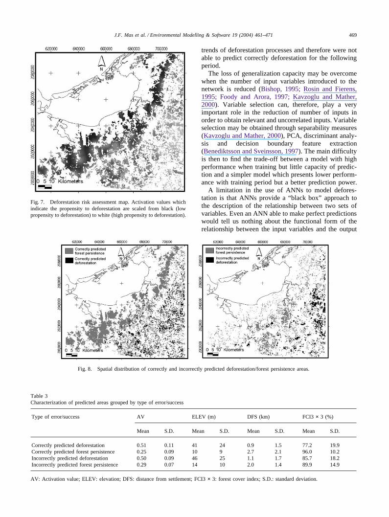
Fig. 8 shows the location of the model’s successes anderrors. By visually inspecting this figure and by calculat-ing characteristics of correctly and incorrectly predictedareas (Table 3), some intuition is gained on what couldbe potential problems and limitations of the currentmodel. The areas incorrectly predicted as forest persist-

468 J.F. Mas et al. / Environmental Modelling & Software 19 (2004) 461–471

Table 1Best measures of separability (Battacharyya distance) and variable combination for subset with increasing number of variables

Number of variables Separability value Best variables combination

1 5.99 (DFS)0.13 (FCI3 × 3)0.02 (MATH)Less than 0.02 All others combinations

2 6.12 (DFS, FCI3 × 3)6.00 (MATH, DFS), (SOIL, DFS), (DISTFE, DFS), (ELEV, DFS), (SLOPE, DFS)5.99 (FCI9 × 9, DFS), (FCI15 × 15, DFS), (DFR, DFS)Less than 0.16 All others combinations

3 6.14 (DFS, FCI3 × 3, ELEV)6.13 (DFS, FCI3 × 3, SOIL), (DFS, FCI3 × 3, DISTFE), (DFS, FCI3 × 3, SLOPE), (DFS, FCI3 × 3,

MATH)Less than 6.13 All others combinations

4 6.15 (DFS, FCI3 × 3, ELEV, DISTFE)5 6.17 (DFS, FCI3 × 3, ELEV, DISTFE, SOIL)6 6.18 (DFS, FCI3 × 3, ELEV, DISTFE, SOIL, MATH)7 6.19 (DFS, FCI3 × 3, ELEV, DISTFE, SOIL, MATH, FCI9 × 9)

DFS: Distance from settlements; DFR: distance from roads; FCI3 × 3: forest cover index (3 × 3 window); ELEV: elevation; DISTFE: distancefrom forest edge; SLOPE: slope; SOIL: soil type; MATH: Matheron index; FCI9 × 9: forest cover index (9 × 9 window); FCI15 × 15: forest coverindex (15 × 15 window). The combinations using more than seven variables did not present separability improvement.

Table 2Three best networks: structure and performance

Number of hidden unitsa Training algorithm Number of epochs used for training Classification accuracy of test data (%)

2 Levenberg–Marquadt 99 61.14 Backpropagation 119 63.18 Backpropagation 257 62.4

a The number of input and output units is the same (three and one) for all the networks.

Fig. 6. MLP structure. It consists of three inputs, one hidden layerwith two nodes and as output the activation value which indicates thepropensity for deforestation (gradient of belonging to the defores-tation class).

ence are large patches of tropical forest in low elevationand correspond mainly to pasture land and rice culti-vation. The areas incorrectly predicted as deforestationare upland fragmented forest. The model over-estimateddeforestation of fragmented upland forest and was notable to predict some large patches of deforestation.These large forest clearing are due mainly to governmentpolicy aimed at increasing rice production in the Stateof Campeche during the 1980’ decade (Isaac-Marquez,1993).

6. Discussion and conclusion

ANNs are able to directly take into account any non-linear relationship between the explanatory and depen-dent variables. According to the Kolmogorov’s theorem,the use of 2n + 1 hidden neurons (with n the number ofinput neurons) can guarantee the perfect fit of any con-tinuous functions (Bishop, 1995). Experiments indicatethat 2n + 1 hidden neurons may be too many in appli-cations and that 2n /3 hidden neurons can generatealmost similar results (Wang, 1994; Li and Yeh, 2002).However, this ability may become a disadvantagebecause the model could be over-specific to the trainingdata. Over-specificity reduces the generalizationcapacities of the ANN. In this study, networks morecomplex, using more input variables, were able to obtainbetter performance when classifying the training datathan the network we selected. But they were not able topredict deforestation of the following period. It seemsthat they were very specific to particular patterns ofdeforestation of the training period, lost the general

469J.F. Mas et al. / Environmental Modelling & Software 19 (2004) 461–471

Fig. 7. Deforestation risk assessment map. Activation values whichindicate the propensity to deforestation are scaled from black (lowpropensity to deforestation) to white (high propensity to deforestation).

Fig. 8. Spatial distribution of correctly and incorrectly predicted deforestation/forest persistence areas.

Table 3Characterization of predicted areas grouped by type of error/success

Type of error/success AV ELEV (m) DFS (km) FCI3 × 3 (%)

Mean S.D. Mean S.D. Mean S.D. Mean S.D.

Correctly predicted deforestation 0.51 0.11 41 24 0.9 1.5 77.2 19.9Correctly predicted forest persistence 0.25 0.09 10 9 2.7 2.1 96.0 10.2Incorrectly predicted deforestation 0.50 0.09 46 25 1.1 1.7 85.7 18.2Incorrectly predicted forest persistence 0.29 0.07 14 10 2.0 1.4 89.9 14.9

AV: Activation value; ELEV: elevation; DFS: distance from settlement; FCI3 × 3: forest cover index; S.D.: standard deviation.

trends of deforestation processes and therefore were notable to predict correctly deforestation for the followingperiod.

The loss of generalization capacity may be overcomewhen the number of input variables introduced to thenetwork is reduced (Bishop, 1995; Rosin and Fierens,1995; Foody and Arora, 1997; Kavzoglu and Mather,2000). Variable selection can, therefore, play a veryimportant role in the reduction of number of inputs inorder to obtain relevant and uncorrelated inputs. Variableselection may be obtained through separability measures(Kavzoglu and Mather, 2000), PCA, discriminant analy-sis and decision boundary feature extraction(Benediktsson and Sveinsson, 1997). The main difficultyis then to find the trade-off between a model with highperformance when training but little capacity of predic-tion and a simpler model which presents lower perform-ance with training period but a better prediction power.

A limitation in the use of ANNs to model defores-tation is that ANNs provide a “black box” approach tothe description of the relationship between two sets ofvariables. Even an ANN able to make perfect predictionswould tell us nothing about the functional form of therelationship between the input variables and the output

470 J.F. Mas et al. / Environmental Modelling & Software 19 (2004) 461–471

layer. The weight matrices of the network do not haveany direct meaning. Numerical experimentation with theANNs may help, however, to identify the most importantvariables and the functional form of the relationshipbetween them and the output(s).

More generally, the limitation of the model are thefollowing: (a) the model is designed to predict only thelocation where land-use change is likely to occur, it doesnot predict the quantity of change and (b) the model doesnot take into consideration the regrowth of forest veg-etation. Training an ANNs with data derived from a landcover change data which present such classes of changecould allow to simulate the different types of changes.However, such modelling will need a more complex net-work (with more outputs), which may result in a loss ofgeneralization capacity.

More general additional limitations of empiricaldeforestation models are that land-cover changes andtheir driving forces are not necessarily found at the samelocation and the intervention of unpredictable factorswhich change deforestation processes. Therefore, themodel is not helpful in providing explanations about theprocesses of change and long-range projections are notreliable. These limitations affect the models indepen-dently of the approach used to establish the relationshipsbetween land use/cover change and explanatory vari-ables. In the study area, main causes of deforestationwere cattle ranching in the first period and rice culti-vation in the second. The effect of the explanatory vari-ables such as human settlement proximity, elevation andforest fragmentation remains similar from a period toanother (Mas and Puig, 2001). However, variation of therelative importance of these explanatory variables overtime leads to errors in predicting the location of defores-tation. Accuracy may be gained developing predictionfor a shorter time and developing models at a coarserscale (Pontius et al., 2001) that will not predict the exactlocation of future clearing but rather the region whereexists a high risk of deforestation.

In this study, the model based on a very simple MLPstructure presents a better performance, expressed as thepower of prediction of deforestation location in the fol-lowing period, than a model elaborated with the samedata by means of a logistic regression, althoughimprovement was not very significant. These results arein agreement with literature data, where performance ofANN has been repeatedly reported to overpass those ofmore traditional method such as regression models (Leket al., 1996; Lek-Ang et al., 1999; Paruelo and Tomasel,1997). ANNs constitute a powerful alternative in spatialland-cover change processes modelling, when more con-ventional models obtain poor performance. However, itis probably impossible to develop models of defores-tation processes, and more generally land use changeprocesses, which present a high power of predictionbecause these processes depend upon very diverse fac-

tors from environmental to socio-economic and culturalthat are changing over time. In the present study, thelocation of forest clearing was predicted with a reason-able precision and the model could be used by environ-mental planners and managers to develop policies aimedat controlling the adverse ecological and social effectsof deforestation.

References

Abdul-Wahab, S.A., Al-Alawib, S.M., 2002. Assessment and predic-tion of tropospheric ozone concentration levels using artificial neu-ral networks. Environmental Modelling and Software 17 (3),219–228.

Almeida, C.M., Batty, M., Monteiro, A.M.V., Camara, G., Soares-Filho, B.S., Cerqueira, G.C., Pennachin, C.L., 2003. Stochasticcellular automata modelling of urban land use dynamics: empiricaldevelopment and estimation. Computers. Environment and UrbanSystems 27 (5), 481–509.

Atkinson, P.M., Tatnall, A.R.L., 1997. Neural networks in remotesensing. International Journal of Remote Sensing 18 (4), 699–709.

Benediktsson, J.A., Sveinsson, J.R., 1997. Feature extraction for multi-source data classification with artificial neural networks. Inter-national Journal of Remote Sensing 18, 727–740.

Bishop, C.M., 1995. In: Neural Networks for Pattern Recognition.Oxford University Press, Oxford, 482.

Bocco, G., Mendoza, M., Masera, O., 2001. La dinamica de cambiodel uso del suelo en Michoacan, Una propuesta metodologica parael estudio de los procesos de deforestacion. Investigaciones Geog-raficas 44 (18), 38.

Chelani, A.B., Chalapati Rao, C.V., Phadke, K.M., Hasan, M.Z., 2002.Prediction of sulphur dioxide concentration using artificial neuralnetworks. Environmental Modelling and Software 17 (2), 159–166.

Civco, D.L., 1993. Artificial neural network for land cover classi-fication and mapping. International Journal of Geographical Infor-mation Systems 7 (2), 173–186.

Cortina Villar, S., Macario Mendoza, P., Ogneva-Himmelberger, Y.,1999. Cambios en el uso del suelo y deforestacion en el sur delos estados de Campeche y Quintana Roo, Mexico. InvestigacionesGeograficas 38, 41–56.

De Brujin, A.C., 1991. Spatial factors in urban growth: towards GISmodels for cities in developing countries. ITC Journal 4, 221–231.

Dıaz Gallegos, J.R., Garcıa Gıl, G., Castillo Acosta, O., March Mifsut,I., 2001. Uso del suelo y transformacion de selvas en un ejido dela Reserva de la Biosfera Calakmul, Campeche, Mexico. Investiga-ciones Geograficas 44, 39–53.

Fontan, J., 1994. Changements globaux et developpement. Nature—Sciences—Societes 2 (2), 143–152.

Foody, G.M., 1995. Land cover classification by an artificial neuralnetwork with ancillary information. International Journal of Geo-graphical Information Systems 9 (5), 527–542.

Foody, G.M., Arora, M.K., 1997. An evaluation of some factors affect-ing the accuracy of classification by an artificial neural network.International Journal of Remote Sensing 18 (4), 799–810.

Geman, S., Bienenstock, E., Doursat, R., 1992. Neural networks andthe bias/variance dilemna. Neural Computation 4, 1–58.

Geoghegan, J., Villar, S.C., Klepeis, P., Mendoza, P.M., Ogneva-Him-melberger, Y., Chowdhury, R.R., Turner, B.L., Vance, C., 2001.Modelling tropical deforestation in the southern Yucatan peninsularregion: comparing survey and satellite data. Agriculture, Ecosys-tems and Environment 85, 25–46.

Grainger, A., 1993. Rates of deforestation in the humid tropics: estimatesand measurements. The Geographical Journal 159 (1), 33–44.

International Geosphere Biosphere Program (IGBP), 1993. Relating

471J.F. Mas et al. / Environmental Modelling & Software 19 (2004) 461–471

Land Use and Global Land Cover Change. In: Turner II, B.L.,Moss, R.H., Skole, D.L. Report no. 24.

Intergovernmental Panel on Climate Changes (IPCC), 1996. ClimateChange 1995, second assessment report. Cambridge UniversityPress, Cambridge, UK.

Isaac-Marquez, R., 1993. Evaluacion del cultivo de arroz como fuentede contaminacion e impacto ambiental para la Laguna de Terminos,Campeche, Mexico. Tesis profesional, Escuela de Biologıa, Univ-ersidad Autonoma de Guadalajara, Mexico.

Jensen, J.R., Qiu, F., Ji, M., 1999. Predictive modelling of coniferousforest age using statistical and artificial neural network approachesapplied to remote sensor data. Ecological Modelling 20 (14),2805–2822.

Kavzoglu, T., Mather, P.M., 2000. Using feature selection techniquesto produce smaller neural networks with better generalisation capa-bilities. In: Proceedings of IGARSS 2000, vol. 7., pp. 3069–3071.

Kim, G., Barros, A.P., 2001. Quantitative flood forecasting usingmultisensor data and neural networks. Journal of Hydrology 246(1-4), 45–62.

Lambin, E.F., 1994. Modelling deforestation processes, a review. EUR15744 EN, TREES series B: Research Report No. 1. Joint ResearchCentre, Institute for Remote Sensing Applications; European SpaceAgency, Luxembourg, Office for Official Publications of the Euro-pean Community, p128.

Lambin, E.F., 1997. Modelling and monitoring land-cover change pro-cesses in tropical regions. Progress in Physical Geography 21,375–393.

Landgrebe, D., Biehl, L., 2000. In: An Introduction to MultiSpec.Purdue Research Foundation, West Lafayette, 168.

Lek, S., Guegan, J.F., 1999. Artificial neural networks as a tool inecological modelling, an introduction. Ecological Modelling 120,65–73.

Lek, S., Delacoste, M., Baran, P., Dimopoulos, I., Lauga, J., Aulanier,S., 1996. Application of neural networks to modelling non-linearrelationships in ecology. Ecological Modelling 90, 39–52.

Lek-Ang, S., Deharveng, L., Lek, S., 1999. Predictive models of col-lembolan diversity and abundance in a riparian habitat. EcologicalModelling 120, 247–260.

Li, X., Yeh, A.G.-O., 2002. Neural-network-based cellular automatafor simulating multiple land use changes using GIS. InternationalJournal of Geographical Information Science 16 (4), 323–343.

Maier, H.R., Dandy, G.C., 2000. Neural networks for the predictionand forecasting of water resources variables: a review of modellingissues and applications. Environmental Modelling and Software 15(1), 101–124.

Manel, S., Dias, J.M., Ormerod, S.J., 1999. Comparing discriminantanalysis, neural networks and logistic regression for predictingspecies distributions: a case study with Himalayan river bird. Eco-logical Modelling 120, 337–347.

Mas, J.F., 1999. Monitoring land-cover changes: a comparison ofchange detection techniques. International Journal of Remote Sens-ing 20 (1), 139–152.

Mas, J.F., Puig, H., 2001. Modalites de la deforestation dans le Sud-ouest de l’Etat du Campeche, Mexique. Canadian Journal of ForestResearch 31 (7), 1280–1288.

Mas, J.F., Sorani, V., Alvarez, R., 1996. Elaboracion de un modelo desimulacion del proceso de deforestacion. Investigaciones Geog-raficas 5, 43–57.

Mas, J.F., Sosa-Lopez, A., Palacio, J.L., Puig, H., 2000. Modellingdeforestation in the region of the Lagoon of Terminos, South EastMexico. In: Proceedings of the ASPRS (American Society ofPhotogrammetry and Remote Sensing) Annual Convention, Wash-ington, DC, May 22–26, 2000,

Mas, J.F., Velazquez, A., Dıaz, J.R., Mayorga, R., Alcantara, C., Castro,R., Fernandez, T., 2002. Assessing land use/cover changes in Mexico.In: Proceedings of the 29th International Symposium on Remote Sens-ing of Environment (CD), Buenos Aires, Argentina, April 8–12, 2002,

Matheron, G., 1970. La theorie des variables generalisees et ses appli-cations. Les Cahiers du Centre de Morphologie Mathematiques deFontainebleau, Fascicule, 5.

Mausel, P.W., Kramber, W.J., Lee, J.K., 1990. Optimum band selec-tion for supervised classification of multispectral data. Photogram-metric Engineering and Remote Sensing 56 (1), 55–60.

Mertens, B., Lambin, E.F., 1997. Spatial modelling of deforestation insouthern Cameroon, spatial disaggregation of diverse deforestationprocesses. Applied Geography 17 (2), 143–162.

Paruelo, J.M., Tomasel, F., 1997. Prediction of functional character-istics of ecosystems: a comparison of artificial neural networks andregression models. Ecological Modelling 98, 173–186.

Pijanowski, B.C., Brown, D.G., Shellito, B.A., Manik, G.A., 2002.Using neural networks and GIS to forescast land use changes: aland transformation model. Computers. Environment and UrbanSystems 26 (6), 553–575.

Pontius, R.G., Cornell, J.D., Hall, C.A.S., 2001. Modelling the spatialpattern of land-use change with GEOMOD2: application and vali-dation in Costa Rica. Agriculture, Ecosystems and Environment 85,191–203.

Puig, H., 2000. Diversite specifique et deforestation: l’exemple desforets tropicales humides du Mexique. Bois et Forets des tropiques268 (2), 41–55.

Rosenfield, G.H., Fitzpatrick-Lins, K., 1986. A coefficient of agree-ment as a measure of thematic classification accuracy. Photogram-metric Engineering and Remote Sensing 52 (2), 223–227.

Rosin, P.L., Fierens, F., 1995. Improving neural network generalis-ation. In: Proceedings of IGARSS 1995, vol. 2., pp. 1255–1257.

Sader, A.S., Joyce, A.T., 1988. Deforestation rates and trends in CostaRica, 1940 to 1983. Biotropica 20 (1), 11–19.

Schneider, L.C., Pontius, 2001. Modeling land-use change in theIpswich watershed, Massachusetts, USA. Agriculture Ecosystemand Environment 85 (1-3), 83–94.

Shahshahani, B.M., Landgrebe, D.A., 1994. The effect of unlabelledsamples in reducing the small sample size problem and mitigatingthe Hughes phenomenon. IEEE Transactions on Geoscience andRemote Sensing 32 (5), 1087–1095.

Soares-Filho, B.S., Pennachin, C.L., Cerqueira, G., 2002. DINAM-ICA—a stochastic cellular automata model designed to simulatethe landscape dynamics in an Amazonian colonization frontier.Ecological Modelling 154 (3), 217–235.

Stephenne, N., Lambin, E.F., 2001. A dynamic simulation model ofland-use changes in Sudano-sahelian countries of Africa (SALU).Agriculture, Ecosystems and Environment 85, 154–161.

Tourenq, C., Aulagnier, S., Mesleard, F., Durieux, L., Johnson, A.,Gonzalez, G., Lek, S., 1999. Use of artificial neural networks forpredicting rice crop damage by greater flamingos in the Camargues,France. Ecological Modelling 120, 349–358.

Turner, B.L., Villar, S.C., Foster, D., Geoghegan, J., Keys, E., Klepeis,P., Lawrence, D., Mendoza, P.M., Manson, S., Ogneva-Himmel-berger, Y., Plotkin, A.B., Perez Salicrup, D., Chowdhury, R.R.,Savitsky, B., Schneider, L., Schmook, B., Vance, C., 2001. Defor-estation in the southern Yucatan peninsular region: an integrativeapproach. Forest Ecology and Management 154, 353–370.

Velazquez, A., Duran, E., Ramırez, I., Mas, J.-F., Ramırez, G., Bocco,G., Palacio, J.-L. Environmental conversion processes in highlybiodiverse areas: the case of Oaxaca, Mexico. Global EnvironmentChange, in press.

Velazquez, A., Mas, J.F., Palacio-Prieto, J.L., Bocco, G., 2002. Landcover mapping to obtain a current profile of deforestation in Mex-ico. Unasylva (FAO) 210 (53), 37–40.

Wang, F., 1994. The use of artificial neural networks in a geographicalinformation systems for agricultural land suitability assessment.Environment and Planning A 26, 265–284.

Yang, G., Collins, M.J., Gong, P., 1996. Multisource data integrationwith neural networks: optimum selection of net variables for litho-logic. In: Proceedings of IGARSS 1996, vol. 4., pp. 2068–2070.