modelling extreme returns in chinese stock market using ...

MODELLING EXTREME RETURNS IN CHINESE STOCK MARKET USING EXTREME VALUE

THEORY AND COPULA APPROACH

A thesis submitted in fulfilment of the requirements for the degree of Doctor of Philosophy

Saiful Izzuan Hussain

BSc Actuarial Science (Universiti Kebangsaan Malaysia)

MSc Applied Actuarial Science (University of Kent)

School of Graduate School of Business and Law

College of Business

RMIT University

July 2016

ii

DECLARATION

I certify that except where due acknowledgement has been made, the work is that of the author alone; the

work has not been submitted previously, in whole or in part, to qualify for any other academic award; the

content of the thesis is the result of work which has been carried out since the official commencement date

of the approved research program; any editorial work, paid or unpaid, carried out by a third party is

acknowledged; and, ethics procedures and guidelines have been followed.

Saiful Izzuan Hussain 14 July 2016

iii

ACKNOWLEDGEMENTS

First and foremost I would thank my lovely wife, Nadiah Ruza. It is quite challenging to

start something new again and far from our beloved family. She is always patient and

willing to sacrifice her desire to make sure I have time for my study. We have also been

blessed with a baby boy, Hatim. Thank you love!

I would like to thank my supervisor, Professor Steven Li, who always gave me good

support regarding my PhD research and writing. He was always a committed supervisor

and shared his knowledge. He always provided me with time for discussion despite his

workload. His guidance and encouragement about the academic world always brought

inspiration to me and helped me to get published in the best journals. This step is

important for my academic career path.

At the same time, I would like to express my gratitude to the Higher Ministry Malaysia and

Universiti Kebangsaan Malaysia (UKM) for their sponsorship. Without it, I would not have

been able to explore this beautiful country, Australia. I have learned a lot from this

country’s culture. This experience is worthwhile to be shared and parts of it would be good

for my country.

There are many fellow doctoral students I would like to thank as well. In my daily work, I

have been blessed with a friendly and cheerful group of fellow students. I appreciated

their advice and feedback in my PhD studies. They always shared their support and

feedback.

I also would like to thank my family in Malaysia. This thesis would not have been possible

without the unconditional love, affection and support of my family: my mother (Mrs

Mariam) who always believed in me; parents in law (Mr Ruza and Mrs Rukiah); and my

relatives. They always supported me and gave me much encouragement during my

study.

Last but not least, special thanks go to my thesis committee for providing me with

encouraging and constructive feedback on the research process.

iv

TABLE OF CONTENTS

Declaration ...................................................................................................................ii

Acknowledgements ...................................................................................................... iii

List Of Figures ............................................................................................................ vii

List Of Tables ............................................................................................................ viii

Abstract ....................................................................................................................... 1

Chapter 1: Introduction .................................................................................................... 3

1.1. Research Background ....................................................................................... 3

1.2. Research Questions and Objectives ................................................................. 8

1.3. Research Significance ...................................................................................... 9

1.4. List of Publications .......................................................................................... 11

1.3. Structure of the Thesis .................................................................................... 12

Chapter 2: Literature Review ......................................................................................... 13

2.1. Chinese Stock Market ..................................................................................... 13

2.2. Extreme Return Distribution ............................................................................ 16

2.3. Dependence Structure with Major Stock Markets around the World ............... 18

2.4. Dependence Structure in the Greater China Economic Area (GCEA) ............ 22

2.5. Summary of Literature Review ........................................................................ 25

Chapter 3: Extreme Value Theory and Copula .............................................................. 26

3.1. Extreme Value Theory .................................................................................... 26

v

3.2. Copula Models ................................................................................................ 30

3.3. Summary ......................................................................................................... 34

Chapter 4: Modeling the Distribution of Extreme Returns in the Chinese Stock Market 35

4.1. Introduction and Literature Review .................................................................. 36

4.2. The Chinese Stock Market .............................................................................. 39

4.3. Data and Sample Statistics ............................................................................. 41

4.4. Methodology .................................................................................................... 47

4.5. Empirical Results ............................................................................................ 51

4.6. Implications for the Chinese Stock Market ...................................................... 62

4.7. Summary and Concluding Remarks ................................................................ 65

4.8. References ...................................................................................................... 68

Chapter 5: The Dependence Structure between Chinese and Other Major Stock Markets

Using Extreme Values and Copulas .............................................................................. 73

5.1. Introduction ..................................................................................................... 74

5.2.Theoretical Background ................................................................................... 77

5.3. Methodology .................................................................................................... 79

5.4. Data and Descriptive Statistics ........................................................................ 85

5.5. Empirical Results ............................................................................................ 89

5.6. Concluding Remarks ..................................................................................... 104

5.7. References .................................................................................................... 106

vi

Chapter 6: The Dynamic Dependence between Stock Markets in the Greater China

Economic Area ............................................................................................................ 111

6.1. Introduction ................................................................................................... 112

6.2. Theoretical Background ................................................................................ 114

6.3. Methodology .................................................................................................. 117

6.4. Data and Descriptive Statistics ...................................................................... 124

6.5. Empirical Results .......................................................................................... 128

6.6. Concluding remarks ................................................................................. 143

6.7. References .................................................................................................... 145

Chapter 7: Summary and Concluding Remarks .......................................................... 150

7.1. Main Findings ................................................................................................ 150

7.2. Limitations and Future Research Directions ................................................. 153

7.3. Conclusions ................................................................................................... 155

References .............................................................................................................. 158

vii

LIST OF FIGURES

Figure 4.1. Daily SSE Composite Index from 2, January 1991 to 31, December 2013 . 42

Figure 4.2. Daily SSE Composite Index from 2, January 1991 to 31, December 2013 . 42

Figure 4.3. QQ plot of daily log returns against the normal distribution ......................... 43

Figure 4.4. L-moment ratio diagrams for the minima series .......................................... 52

Figure 4.5. L-moment ratio diagrams for the maxima series ......................................... 52

Figure 4.6. A comparison of the normal, GEV and GL distributions .............................. 65

Figure 5.1. Relative daily index levels over the sample period…………………………...86

Figure 5.2. Upper tail distributions ................................................................................. 93

Figure 5.3. Fitted overall distributions ............................................................................ 94

Figure 6.1. Relative daily index level ………………………………………………………124

Figure 6.2. Daily returns for GCEA stock markets ....................................................... 126

Figure 6.3. Upper tail of GCEA markets’ residuals ...................................................... 131

Figure 6.4. Lower tail of GCEA markets’ residuals ...................................................... 132

Figure 6.5. Fitting residuals for the GCEA stock markets ............................................ 132

Figure 6.6. Evolution of the dependence parameters .................................................. 138

viii

LIST OF TABLES

Table 4.1. Descriptive Statistics .................................................................................... 45

Table 4.2. Parameter estimates for GEV distribution .................................................... 53

Table 4.3. Parameter estimates for GL distribution ....................................................... 54

Table 4.4. Parameter estimates for GEV distribution before and after stock movement

restriction… ................................................................................................................... 56

Table 4.5. Parameter estimates for GL distribution before and after stock movement

restriction ....................................................................................................................... 57

Table 4.6. Parameter estimates for GEV distribution during GFC ................................. 59

Table 4.7. Parameter estimates for GL distribution during GFC .................................... 60

Table 4.8. Probability (%) of obtaining a daily return within specific intervals for the lower

tail.................................................................................................................................. 63

Table 5.1. Descriptive statistics of daily returns……………………………………………87

Table 5.2. Linear correlation table ................................................................................. 88

Table 5.3. The estimated parameters for the tails based on GPD ................................. 90

Table 5.4. Parameter estimates for constant and time-varying copulas ........................ 96

Table 6.1. Descriptive statistics of daily returns…………………………………………..127

Table 6.2. Linear correlations between markets .......................................................... 128

Table 6.3. The parameter tails fitted by GPD .............................................................. 129

Table 6.4. Parameter estimates for constant and dynamic copulas ............................ 134

ix

Table 6.5. Model comparison: constant vs. dynamic copulas ..................................... 142

1

ABSTRACT

The Chinese stock market has unique features that make it a challenging and interesting

research topic. It is one of the biggest stock markets in the world in terms of capitalization

yet it is still considered to be an emerging market. This market is very volatile and thus

displays some extreme behaviour. Extreme movements in share returns rarely occur.

However, they can have devastating consequences. Thus, it is important for investors,

speculators and risk managers to comprehend extreme movement events in stock

markets. To this end, we employ Extreme Value Theory (EVT) and copulas in this study.

First, we are concerned with the distribution of the extreme daily returns of the Chinese

stock market. Generalized Extreme Value (GEV), Generalized Logistic (GL) and

Generalized Pareto (GP) distributions are three well-known distributions in extreme value

theory. These distributions are used to identify the distribution which is best fitted with the

extreme returns. Our results indicate that the GL distribution is a better fit for the minima

series and the GEV distribution is a better fit for the maxima series based on daily returns

in the Chinese stock market from 1991 to 2013. This is in contrast to the previous studies,

such as the one in the US and Singapore stock markets. This finding also considers

extreme events that occurred and could potentially impact on the Chinese stock market

such as the introduction of stock movement restriction and the Global Financial Crisis

(GFC). Our results are robust regardless of these extreme events.

Second, this study explores the dependence structure between the Chinese stock market

and other major stock markets. This study reveals that the Chinese stock market seems

to be more strongly integrated with stock markets in Australasia than Europe or the United

States. It is shown that the dependence between Chinese stock market and those of other

stock markets is stronger during the crisis period than a normal period. This study also

suggests that not much benefit can be gained during a downturn in portfolio diversification

across the pairs of stock markets considered.

2

Third, this study examines the dependence structure between the stock markets in the

Greater China Economic Area (GCEA) including mainland China, Hong Kong and

Taiwan. These stock markets have become more and more important in recent years.

However, little is known about the dependence structure between these markets. This

research reveals that the dependence between all pairs of GCEA stock markets is strong.

As expected, the Shanghai-Shenzhen pair has the strongest dependence (overall, lower

tail and upper tail) among all pairs considered. This is followed by the Hong Kong-Taiwan

pair. This study finds that diversification is effective for two pairs (Shenzhen-Hong Kong

and Hong Kong-Taiwan) in the context of negative market extreme events.

Overall, this study reveals some important results regarding the extreme behaviour in the

Chinese stock market. This study also demonstrates that combining EVT and copula can

provide an effective way to understand extreme behaviour in stock markets. This

approach can lead to incremental insights to the conclusions based on the normality

assumption. The outcome of this study can have important implications for policy-making

and risk management.

3

CHAPTER 1: INTRODUCTION

1.1. Research Background

Chinese stock market is the largest emerging stock market in the world. It has grown

enormously over the past two decades since the 1990s. Continuing economic reforms

and liberalization undertaken by the Chinese authorities in recent years have stimulated

the development of the Chinese financial markets (Chan et al. 2007; Lien and Chen

2010). The Chinese stock market has surpassed Japan based on market capitalization

since 2007 and has become the most influential stock market in the Asian region. It has

become the second largest stock market in the world behind the US stock market.

In contrast to developed markets where institutional investors take the leading role, major

participants in the Chinese stock market are individual investors. These investors tend to

bet on speculative returns rather than viewing the stock market as a long-term investment.

Many finance-related studies have been done in this market. However, analyses

regarding the extreme return behaviour for this market have been limited.

The information regarding extreme return behaviour in the stock market is still poorly

understood. Most studies have examined developed countries such as the US, the UK

and Japan. In contrast, this research investigates the extreme returns behaviour in the

Chinese stock market. The aim of this research is to understand the distribution of

extreme returns in this market. It will also explore how this market is integrated with others

using advanced tools in risk management.

Extreme behaviour has become an important consideration for investors, regulators and

risk managers. The behaviour of extreme returns can impact on the performance of the

stock market significantly, reduce the benefits of risk diversification and affect the stability

of the financial system, as can be seen in the Global Finance Crisis (GFC) during 2007

and 2008. The GFC had forced many reputable and large firms to face survival problems

4

and bankrupted many of them (e.g. AIG, Lehman Brothers and Merrill Lynch). Most of the

stock markets were affected badly during this period. It should be noted that emerging

markets have experienced greater volatility and financial instability during the GFC.

The GFC has brought the entire risk management system into question. Following the

market crash in late 2008, it has become very critical for financial institutions, regulators

and academics to develop models that consider and guard against the extreme

behaviour.

Early studies have shown many large financial institutions adopted a conservative model

to measure the risk. The most well-known risk measure is Value at Risk (VaR) has been

used as an industrial standard risk measure for market risk measurement. This tool has

again attracted global attention for its accuracy and therefore, is necessary to have such

models that are able to estimate the risk under different market conditions (for example,

with or without a financial crisis).

VaR can be defined as the maximum loss which may be incurred by a portfolio, at a given

time horizon and a given level of confidence. VaR has been recognized by both official

bodies and private sector groups as an important market risk measurement tool. Many

official bodies have embraced the concept of VaR. These include the Basel Committee

on the Banking Supervision (Supervisions (1998)) and the Bank for International

Settlements (Fisher-Report, 1994). The Group of Thirty (1993), a private sector

organization which consists of bankers and other derivatives market participants, has

advocated the use of VaR for setting risk management standards. Risk Metric that is used

for estimation of VaR was first introduced in 1994 by JP Morgan Bank. Since then many

methods of estimating VaR have been proposed. For more information on VaR and its

estimation, we refer to Jorion (2000).

The important issue for VaR is the distribution function that used to present the returns of

the asset. Usually, as allowed by the Basel Committee, a normal distribution is used as

the assumption for return distribution. A normal distribution is a popular assumption that

has been used to model extreme behaviour. However, research has consistently shown

that financial returns tend to have fatter tailed returns than the normal distribution. This

5

indicates that extreme losses (or gains) have a higher probability of occurring compared

to those implied when the normal distribution is employed. This means that the model

based on normality assumption can be inaccurate and fail to predict a catastrophic event.

Therefore it is important to know the best distribution incorporating the fat tail behaviour.

For this study, one of the objectives is to identify the best distribution that fits with the

extreme returns of the Chinese stock market. In the financial market, it is important to

quantify extreme losses in current market conditions. This is important for VaR

calculation. With growing turbulence in the financial markets worldwide, evaluating the

probability of extreme events like the Asian Financial Crisis (AFC) and GFC has become

an important issue in financial risk management. This is where Extreme Value Theory

(EVT) can play a major role.

EVT provides a comprehensive theory based on statistical models to describe extreme

scenarios. EVT techniques are widely used in areas such as weather, hydrology and the

environment. EVT is also a well-known technique in many fields of applied sciences

including insurance and engineering. It was first applied in finance in the late 1980s by

Parkinson (1980).

Second, this thesis is concerned with the dependence structure between Chinese stock

market and other major stock markets. The significant increase in market capitalization

of the Chinese stock market in recent years has become one of this research motivation

to study this behaviour. The Chinese stock market has been increasingly integrated with

many markets as pointed out in many previous studies. Therefore a crash or boom in this

market is likely to have a contagious effect on another one. This could lead to a huge

disaster. In addition, it will be interesting to see the dependence structure between the

Chinese stock market with others during the financial crisis periods.

Although extensive studies have been carried out on dependence, there is not much

published work regarding fat tail modelling and extreme returns behaviour for the Chinese

stock market. Most studies tend to focus on the developed market. The dependence

structure between the Chinese stock market and other markets has important implications

for risk management, portfolio diversification and international diversification.

6

The Pearson coefficient is a tool that can be used to compute dependencies of financial

asset returns. However, it has several limitations. Several studies showed that asset

returns rarely follow a normal distribution. Furthermore the correlation among financial

assets is non-linear. The extreme movements that occur due to economic shocks will also

make the modelling of co-movement among asset returns a difficult challenge.

This study uses copula to overcome the shortcomings of simple linear correlation. Recent

studies show that copula can serve as an alternative for modelling correlations in terms

of the asymptotic dependence and characterization of nonlinearity. Copula is used to

model multivariate distribution functions of random variables using flexible marginal

distribution functions of each random variable set. Compared to traditional methods for

estimating dependence, copula can be a very powerful tool. In this thesis, all returns

empirically show non-normal behaviour. Overall dependence and tail dependence are

examined in detail. All these features make copula approach a better method to

understand the behaviour of each stock market pair than the traditional correlation

method.

This research aims to fill the gap in investigating the dependence structure between the

Chinese stock market and other major stock markets by focusing specifically on the lower

and upper tails. The combination of EVT and time-varying copula has several advantages

that help to model the dependence structure between Chinese stock market with others

more accurately. In turn this will improve the ability to manage risks in the future and

improve our understanding of the behaviour of this emerging market from an international

perspective.

Concerning regional dependence, there is evidence showing that local events can cause

country-specific stock price reactions. Specifically, most of the volatility in the stock

markets can be related to the economic, political and social events that happen in its

region. This research will examine the dependence structure in the Greater China

Economic Area (GCEA). At the same time, the dependence structure between GCEA has

not been treated in much detail. The upper and lower tail dependence between GCEA

stock markets are interesting and should be explored further, as they may contribute in

7

different ways compared to developed countries’ stock markets. The results can provide

evidence as to whether the findings from developed stock markets are valid to Chinese

stock market.

Overall, this research aims to employ EVT and copula approach to provide a better

understanding of extreme behaviour in the Chinese stock market to fill the gap in our

knowledge concerning this topic. The contribution of this study is to understand the

behaviour of extreme returns of the Chinese stock market regarding the type of

distribution and dependence structure. The findings have important implications for both

asset pricing and financial risk management in the Chinese stock market.

8

1.2. Research Questions and Objectives

This research has several objectives to fill the gap in the literature. It aims to:

I. Identify the best distribution for the extreme returns in the Chinese stock market.

II. Understand the dependence structure between the Chinese stock market and

other major stock markets around the world.

III. Understand the dependence structure between stock markets in the Greater China

Economic Area (GCEA).

The following research questions are developed according to the research objectives

above:

I. What is the best fit distribution for the extreme returns in the Chinese stock market?

II. How does Chinese stock market correlate with other major stock markets around

the world?

III. How strong is the dependence structure between stock markets in the Greater

China Economic Area (GCEA)? Does the dependence structure of GCEA stock

markets have strengthen over the years?

9

1.3. Research Significance

This research contributes to the literature in the following ways. First, the research aims

to assess empirically the behaviour of extreme returns in the Chinese stock market by

using both EVT and copula. Normality models are often ill-suited to deal with the extreme

circumstances that arise in the financial market, especially in emerging markets.

Increasing interests in emerging markets have provided the impetus for both adaptations

of the current model that considers this behaviour. .

Second, this research will explore and analyse the dependence of the Chinese stock

market with other major stock markets. The international equity markets have become

increasingly volatile and integrated. The dependence that existed between financial

markets has always been one of the crucial issues in finance and investment field. For

instance, any political tension that happens in the Chinese stock market is likely to affect

returns on most stocks in Hong Kong. However, this will not likely wield much influence

on the stock market in Ukraine. In contrast, war or political tensions in Russia may have

an effect on Ukraine’s stock market (since both of them have strong economic ties and

are neighbours) more likely, but have little effect on Hong Kong or Chinese stock market.

International portfolio diversification has emerged as one of the key strategies to achieve

higher returns compared to domestic market investment alone. This outcome provides

useful information for investors in the Chinese stock market who wish to seek another

way to diversify their international portfolios and assets. Therefore it is valuable to study

the behaviours of the dependence structure empirically.

Third, this study will also contribute to the literature on dependence between GCEA stock

markets. So this research contributes to the increasing portfolio diversification and

improves active asset allocation of investors interested in this area. Investors can use the

results to adjust the asset allocation dynamically to achieve optimal portfolio since the

dependence structure between Chinese stock market and others might differ.

10

Fourth, this research explores the application of EVT and copula models to the risk

management process. This study addresses the crucial issues by empirically exploring

the effectiveness of EVT and copula in managing portfolios risks in this market for

selected areas. It is believed that copula can provide more information on the dependence

structure over time compared to the traditional method. The result can improve the

confidence of forecasting regarding the volatility persistence and asymmetry of returns.

From a theoretic perspective the results of the extensive empirical study may indicate

promising directions for further development of theoretical risk modelling. This method

provides new insight on understanding the extreme behaviour of and the dependence

structure between stock markets.

Overall, this study will potentially have important implications for risk management. This

research will contribute to the topic of VaR estimation and international diversification

between the Chinese and other stock markets. Results can be useful for practitioners in

portfolio risk management.

11

1.4. List of Publications

The following are publications arising from this thesis:

Journal papers

Hussain, S. I., & Li, S. (2015). Modeling the distribution of extreme returns in the Chinese

stock market. Journal of International Financial Markets, Institutions and Money, 34, 263-

276.

Hussain, S. I., & Li, S. (2016). The dependence structure between Chinese and other

major stock markets using extreme values and copulas. Under review by International

Review of Economics & Finance.

Hussain, S. I., & Li, S. (2016). The Dynamic Dependence between Stock Markets in the

Greater China Economic Area. Under review by Review of Pacific Basin Financial

Markets and Policies.

Peer reviewed conference paper

Hussain, S. I., & Li, S. (2015). Modeling International Diversification between the Chinese

Stock Market and Others. In 2015 Financial Markets & Corporate Governance

Conference.

12

1.3. Structure of the Thesis

The remainder of the thesis consist of six chapters described below.

Chapter 2 reviews the literature on the Chinese stock market, extreme distribution and

dependence structure of the stock markets. This chapter reveals several research gaps

regarding extreme returns behaviour in the Chinese stock market.

Chapter 3 describes the research methodology used in this thesis. The studies on EVT

and copula approaches are discussed in this chapter.

Chapter 4 focuses on modelling the extreme returns in the Chinese stock market. This

chapter reproduces in full a scientific paper that has been published in the Journal of

International Financial Markets, Institutions and Money in January 2015. This particular

chapter attempts to identify the best extreme returns distribution for the Chinese stock

market.

Chapter 5 provides an empirical analysis and results regarding the dependence structure

between Chinese stock market and other major stock markets including US, Canada, UK,

Japan, Germany and Australia are studied. This paper is under review by International

Review of Economics & Finance.

Chapter 6 is an analysis of the dynamic dependence structure between the stock markets

in Greater China Economic Area (GCEA). This study describes and discusses the

empirical dependence structure between the stock markets of Shanghai, Shenzhen,

Hong Kong and Taiwan. This paper is under review by the Review of Pacific Basin

Financial Markets and Policies.

Chapter 7 provides an overall summary of this thesis and its major findings. Lastly, the

limitations of this study, areas for further research, and final concluding remarks are also

given.

13

CHAPTER 2: LITERATURE REVIEW

This chapter begins with a review of the literature on the Chinese stock market in Section

2.1. From this background literature, the review then focuses on extreme return

distribution in Section 2.2. In Section 2.3, the literature regarding the dependence

structure of the Chinese stock market and others is discussed. Section 2.4 is about the

literature on the dependence structure between GCEA stock markets. A summary of the

overall literature review is presented in Section 2.5.

2.1. Chinese Stock Market

Since its establishment in the early 1990s, Chinese stock market has experienced

tremendous economic growth over the past two decades in terms of capitalisation, the

number of listings and turnover. Based on data released by the China Securities

Regulatory Commission (CSRC), the number of domestic listed companies on October

2015 is 28001.

There are two major stock exchanges that are associated with the Chinese stock market;

the Shanghai Stock Exchange (SHSE) and Shenzhen Stock Exchange (SZSE). Both of

these stock exchanges started trading in 1990. In 2015 the total market capitalization of

the Shanghai Stock Exchange was approximately 18,238 billion RMB while the total

capitalization of Shenzhen Stock Exchange 12,22 billion RMB. There are a few

differences in the Shanghai and Shenzhen stock exchange systems. Most companies

that are listed on SHSE are state-owned and large. In comparison, those companies on

the SZSE are joint-ventures, small and export-oriented. The relative size of these markets

1 See http://www.csrc.gov.cn/pub/csrc_en/marketdata/security/monthly/201511/t20151124_287067.html, accessed on 1 December

2015.

http://www.csrc.gov.cn/pub/csrc_en/marketdata/security/monthly/201511/t20151124_287067.html

14

has also changed. In 1992, SHSE was relatively small and less active than SZSE but this

changed due to a shift in government policy by the end of 1994. This difference could

lead to markedly different outcomes (Hilliard and Zhang 2015). Both exchanges operate

five days a week except on holidays. SHSE tends to have fewer holidays compared to

SZSE.

The Chinese stock market has many interesting features. There are two types of shares

on the Chinese stock market: firstly, A Shares (restricted to domestic investors only); and

secondly, B Shares (available to both domestic and foreign investors). Another interesting

feature is a limit of 10% of the daily movement in share price since 16 December 1996.

This limitation was introduced to curb excessive volatility in this market. Indeed, about

70% of shares are non-tradable and this stock is held by the government, state-owned

enterprises (SOEs) and Chinese institutions (Mookerjee and Yu 1999).Thus this

characteristic enables the Chinese government to wield much influence on the Chinese

stock market compared to governments in developed markets. It also means the

governments can hugely impact on the stock market price movements.

This stock market is also quite different compared to those in developed countries

regarding exchange facilities. Chinese stock market strictly prohibits the practice of short

sale trading. Therefore, the supply of shares is limited and affects the stock price

formation limit. The behaviour of the Chinese stock market is very different from

developed countries’ stock markets. This market has long posed a challenge for finance

studies.

Major market participants in this market are individual investors. A-share individual

accounts are about 57.59 million and institutional ones number approximately 1.35 million

accounts for investors2. This indicates there are many unsophisticated individual

investors in this market. It also suggests that most investors lack qualified security

analysts in the Chinese stock market compared to the developed stock markets (Yao et

al. 2014). Individual investors can behave like noise traders as they have low

2 Source, the websites of SSE and SZSE: www.sse.com.cn and www.sse.org.cn

http://www.sse.com.cn/

http://www.sse.org.cn/

15

transparency and invest more often according to rumour and past trends (Kang et al.

2002).

Many actions have been taken by Chinese authorities to liberalize the Chinese stock

market. At an early stage, B-shares were a platform that designed for foreign investors

and was denominated in the Chinese local currency, the Renminbi (RMB), which was

payable in foreign currency. A-shares have been actively traded by domestic investors.

In contrast the trading of B-shares (shares subscribed and traded in foreign currency) is

very small. However, a domestic trader could invest in B shares and this is payable in US

dollars due to changes in the regulations in 2001. This has contributed to the price of B-

shares rising significantly since the regulations were introduced. The removing of the

restriction has attracted more foreign investments (Chan et al. 2007).

Another attempt by Chinese authorities to liberalize the Chinese stock market occurred

through the Foreign Institutional Investors (QFII) programme in December 2002. This

programme allows licensed foreign institutional investors to trade A-shares on the market.

After the successful introduction of this programme, trading in A-shares was opened to

individual foreign investors on 9 July 2003.

The Chinese authorities also launched the QDII programme in May 2006. This

programme permits licensed domestic institutions to invest in overseas stock markets.

These changes are expected to increase the dependence between the Chinese stock

market and others (Li 2012). All of these liberalization attempts have created greater

international links between the Chinese stock market and those of other countries (He et

al. 2014).

To conclude, many initiatives have been taken to boost this market by the Chinese

government. Since then it has become one of the main markets favoured by international

investors. The Chinese stock market is the largest emerging market in the world and is

different in various ways from stock markets in developed countries. Chinese stock

market is still developing and highly regulated by the government.

16

2.2. Extreme Return Distribution

A large and growing body of literature on the Chinese stock market has been published

in recent years. This research fills several gaps in the literature review regarding extreme

returns behaviour. To the best of our knowledge, little is known about Chinese stock

market extreme behaviour. Most studies tend to focus on the centralized data and neglect

the facts of financial data.

EVT study has renewed interest in analyzing the behaviour of the tails. Extreme returns

can be defined as the minimum daily return (the minima) or the maximum daily return (the

maxima) of a stock market index over a given period (selection interval) according to

Longin (1996).

Parkison (1980) was one of the first to apply EVT in finance and found the tail distribution

contained information able to predict a crash. Jansen and De Vries (1991) calculated the

probabilities of crashes and booms by estimating the tail index based on the information

that determined the fatness of the tails of the distribution of returns. More details regarding

EVT can be found in McNeil (1998), Straetmans (1998), Jondeau and Rockinger (1999),

McNeil (1999), Rootzen and Kluppelberg (1999), Danielsson and De Vries (2000), McNeil

and Frey (2000), Neftci (2000), and Gencay et al. (2003).

Longin (1996) found extreme returns in the US can be assigned using (Generalized

Extreme Value (GEV)) distribution for both the minima and maxima series. This finding

was also reported by Jondeau and Rockinger (2003) and Gençay and Selçuk (2004).

However, studies by Gettinby et al. (2004,2006) found that the Generalized Logistic (GL)

distribution is the best distribution that fits the extreme daily stock returns in the US, UK

and Japan compared to the GEV distribution. GL distribution also can be used to calculate

VaR accurately compared to the GEV or normal distribution. A study by Tolikas and

Gettinby (2009) indicates that Singapore’s stock market is fitting best with the GL

distribution compared to the GEV and normal distribution. GL distribution is able to

describe the extreme returns for the minima and maxima series adequately compared to

the GEV distribution for selected intervals of their study.

17

Since the markets are very volatile, the need for modelling the distribution tails is very

apparent. It was concluded that most markets are not characterized by normality and can

be described within an extreme value theory frame. Since VaR estimations focus mainly

on the tails of a probability distribution, techniques from EVT may be particularly effective

for extreme observations. Estimation of VaR using EVT offers major improvements over

well-known methods for oil market (Marimoutou et al. 2009).

Furthermore, Bali (2003) and Straetmans et al. (2008) indicated that EVT models provide

better estimation than the standard approach, which assumes a normal distribution. More

recent application of VaR using EVT has been done by Allen et al. (2013), Karmakar

(2013) and others. More studies on estimation of VaR using EVT can be found in Bradley

and Taqqu (2003) and Brodin and Kluppelberg (2008). All of this emphasizes the

importance of understanding the extreme behaviour returns before they are implemented

for the purpose of VaR measurement.

To this end, this study uses EVT to study the tail behaviour of the Chinese stock market.

The best distributions that fit well with the minima and maxima series in Chinese stock

market are studied in this thesis.

18

2.3. Dependence Structure with Major Stock Markets around the World

This purpose of this section is to review the literature on the dependence structure of

Chinese stock market with those of other countries. China has built a close relationship

with the rest of the world regarding international trade and investment. This integration is

due to the Chinese government opening its doors to foreign investment and cross-border

listings (Sun et al. 2009). Therefore, any change in the Chinese economy or stock market

could impact on others.

Over the past decade, there has been a dramatic increase in dependence studies. Chan

et al. (2007) have shown that the Chinese stock market is now more integrated with

developed markets. A study on inter-Asian-Pacific dependence by Hyde et al.

(2007) showed there is a strong correlation between Asian-Pacific countries, Europe, and

the US. However, a study by Li (2007) discovered that the Chinese stock market is

weakly integrated with regionally developed markets. This is echoed by Lai and Tseng

(2010) which show there are no significant dependencies between Chinese stock market

and the G7 countries.

The dynamic dependence structures between the Chinese and US financial markets are

quite volatile according to Hu (2010). Recent evidence suggests that there is significant

mutual feedback of information between domestic (Hong Kong) and offshore (New York)

markets in terms of volatility and pricing according to Xu and Fung (2002). The volatility

linkages between Chinese stock market, Hong Kong and the US using daily data with a

multivariate GARCH framework has been demonstrated by Li (2007). The study showed

the spillover effects from Hong Kong to Shanghai but not any between the Chinese stock

market with the US stock market. According to Rosch and Schmidbauer (2008) the

Chinese stock market appears to be immune to extreme external movements. However,

the dependence structure of Chinese stock markets has increased after 2000. The study

also shows that a sharp downward movement in the US stock market is more likely to

impact the Chinese stock market during a bear period than during a bull period in the US.

According to George (2014), the interaction between the Chinese stock market and US

stock market has been improved recently. This study also demonstrates US stock market

19

can forecast Chinese stock market. However, the Chinese stock market has not shown

the similar ability to forecast Us stock market.

Next, previous studies also suggest that the tails of return distributions are fatter than

normal while the correlations are asymmetric across downside and upside market

movements. (e.g. Longin and Solnik 2001; Ang and Chen 2002; Kolari et al. 2008).

Therefore, finding a more suitable approach to modelling dependencies between stock

returns has become a significant challenge in risk management. One possible solution

is to apply the dynamic conditional correlation (DCC) model proposed by Engle (2002)

and Engle and Colacito (2006). The family of DCC methods considers the time-variation

issue, but does not account for extreme value and departure from normality. Silvennoinen

and Terasvirta (2009) and Tsafack (2009) discovered that DCC family models could lead

to bias in the estimations used in portfolio management with the presence of asymmetry

in a tail correlation. Therefore it would be inappropriate to apply DCC models.

Recent studies show that copula can serve as an alternative method to overcome the

limitations of the nonlinearity method. Copula is a risk management tool that models the

dependence structure between variables and was first used in finance in the early 2000s

(Cherubini et al. 2004). Specifically, copula is a technique used to understand the

dependence structure and consideration of nonlinearity without the constraints of

normality. It can separate marginal behaviour of variables from the dependence structure

through the use of joint distribution function. The assumption of normality used in most of

the financial data makes measuring the dependence structure of market returns between

two series less accurate. Thus copula can be a better tool for modelling financial data.

There are many types of copula that can be used to fit the different scenarios. Most

empirical studies have focused on the equity risk and employ Gaussian copula and t

copula. A study by Hsu et al. (2012) focused on Gaussian, Gumbel and Clayton copula

on Asian markets while Wang et al. (2010) in their study use Gaussian, t and Clayton

copula to describe a portfolio risk structure. In Cherubini and Luciano (2001) an

Archimedean copula family is employed and the historical empirical distribution in the

estimation of marginal distributions for VaR estimation. Rockinger and Jondeau (2001)

20

utilized the Plackett copula and proposed a new measure of conditional dependence. De

Melo Mendes (2005) investigated the extreme asymmetric dependence in daily returns

for seven emerging markets using extreme value copula functions.

This study uses Symmetric Joe Clayton (SJC) copula to model the dependencies

between the assets returns. SJC copula is a modification of the “BB7” copula of Joe

(1997). This type of copula provides more information regarding tails information.

According to Patton (2006a), SJC copula is more efficient at modelling the dependencies

between the financial markets. In contrast to Gumbel and Clayton, SJC copula can

capture the lower and upper tails at the same time. SJC copula does not impose

symmetric dependence on the variables like the Gaussian copula does. This type of

copula is able to capture the upper and lower tail dependence of joint distribution at the

same time. Bhatti and Nguyen (2012) used SJC copula to examine the dependence

structure across financial markets, including Australia, the US, the UK, Hong Kong,

Taiwan, and Japan. In another analysis by Nguyen and Bhatti (2012), they investigated

the dependence between two stock exchanges, those of China and Vietnam where

indices concerning oil prices utilized copula functions.

The recent extension of the unconditional copula theory to the conditional case has been

used by Patton (2006a) to model time-varying conditional dependence. This research

focuses on time-varying copula based the work over these recent years by Patton(2006a)

and Jodeau and Rockinger (2006).This method allows the temporal variation in the

conditional dependence in time series, making it more dynamic and time sensitive. For

an application, Bartram et al., (2007) have used time-varying conditional copula to study

the integration of seventeen European stock market indices.

However, the study might ignore fat-tail phenomena especially for the series. Using EVT

with copula is one promising solution in addressing the fat-tailed and nonlinearity issues.

The study of copula and EVT has been done by Clemente and Romano (2003), de Melo

Mendes and de Souza (2004), Hotta et al. (2006), Hsu et al. (2012) and Wang et al.

(2010).

21

Clemente and Romani (2003) have used copula and EVT approaches to model

operational risk using insurance data. De Melo Mendes and Souza (2004) in their study

focus on crises scenarios while Hotta et al. (2006) used the copula approach to model

market risk for a portfolio consisting of Nasdaq and S&P 500 indices. These are

considered to be typical of developed markets. Hsu et al. (2012) incorporate a

combination of copula and EVT to access portfolio risk in six Asian markets. Wang et al.

(2012) employed copula and EVT to analyse the risk of foreign exchange portfolios.

Our study differs from these studies in several respects. The interest in emerging markets

has arisen out of the need to develop a new model and adapt current models to new

circumstances. The different economic systems governing these markets allow this

research to observe the impact of economic structures on financial dependencies. China

is a manufacturing country and now has the largest emerging stock market in the world.

The dependence levels of this market are quite interesting to see and compare and results

will help investors to identify the opportunities for international portfolio management.

In summary, there are not many details or answers concerning the dependence structure

between Chinese and other major stock markets and the results tend to be mixed. It is

hard to find any systematic research that has been done on Chinese stock market

dependence under extreme setting. The study of extreme returns and integration between

EVT and copula has not had much detail. Furthermore, research on the subject has been

mostly restricted to the developed stock markets. This research seeks to remedy these

problems by using the EVT and copula approach.

22

2.4. Dependence Structure in the Greater China Economic Area (GCEA)

This section examines the context of dependence in the Greater China Economic Area

(GCEA). Chinese stock market is one of the world’s major stock markets. While Taiwan

is one of the top ten stock markets in the world. Most companies based on technology

originate in Taiwan, for example Asus. Acer Inc, HTC Corporation. Hong Kong is one of

the five major stock markets in the world and the main gateway to Chinese stock market

for international investors. These markets combined is huge in terms of market

capitalization.

The economic exchange within this stock market is strong despite political tensions.

Based on trading activities, mainland China is Taiwan’s largest import and export

destination. Mainland China accounted for 26.8% of Taiwan's exports and 15.8% of its

imports in 2013. Mainland China is also the main export and import partner of Hong Kong.

Its exports account for 59.9% and imports are 41.5% of Hong Kong’s in 20133.

Aggarwal et al. (1999) showed that local events can cause specific stock price reactions.

Their study showed that most of the increasing volatility in the emerging market could be

linked to economic, social and political events. Nikkinen et al. (2008) found that the impact

of extreme events leads to significant increases in volatility across and throughout certain

regions. This has implications for the international economy as well. A study by Zhou et

al. (2014) showed the volatility of the Chinese stock market has ominously impact on

other markets since 2005. However, the volatility interactions among the GCEA stock

markets were more prominent than all major stock markets. Thus, it is quite interesting to

examine for the dependence between the stock markets in the GCEA as they also share

similar cultural, geographical and social ties.

The information regarding dependence structure of GCEA stock markets could have

implications on diversification and portfolio management. It is important to understand

how these markets relate to each other in terms of the stock market dependence

3 Data sourced from http://www.dfat.gov.au

http://www.dfat.gov.au/

23

structure. As dependence structure between GCEA might differ over the time, the results

could be used by investors to manage the assets dynamically to achieve optimal asset

allocation. At the same time, there is the possibility of diminishing benefit from asset

diversification as dependence structure of GCEA stock markets might strengthen over

the years.

There are not many studies regarding dependence between GCEA stock markets. Liu

and Sinclair (2008) suggested that movements in stock prices in GCEA were determined

by economic fundamentals which could be related to the regional area. Johansson and

Ljungwall (2009) found that a spill-over effect exists between the GCEA stock markets.

There is more integration between the GCEA stock markets (Cheung et al. 2003). This

study focused on the macro levels of the economy such as exchange rates, interbank

rates, and prices. Cheung et al. (2005) also studied how the GCEA finance market

integrates with other economies in their later study. The dependence is more marked after

the Asian crisis (Groenewold et al. (2004)). Hong Kong is one of the most influential of

the GCEA markets according to Cheng and Glascock (2005). However, this position is

threatened by fast-growing of Shanghai Stock Exchange (Wang et al. 2012).

Another interesting study was conducted by Wang and Iorio (2007). They showed that a

strong correlation existed between China’s A-share market and Hong Kong’s stock

market. According to Yang and Lim (2004), the Hong Kong stock market has become the

main gateway between the Chinese stock market and others. This platform has

contributed to enhancing the transmission of information and interaction between the

Chinese stock market and those of other countries. There are substantial capital flows

into the Chinese stock market via the Hong Kong stock market. The results might be

different with other; e.g. Taiwan GCEA stock market.

In contrast, Groenewold et al. (2004) found Chinese stock market is relatively isolated

from Hong Kong and Taiwan stock market. The evidence demonstrates that Hong Kong

has a weak predictive power for returns in the Chinese stock market during the crisis;

AFC. This is confirmed by Ho and Zhang (2012) that demonstrated the Chinese stock

market is less volatile than the Taiwan and Hong Kong stock markets.

24

He et al. (2009) demonstrated that the Hong Kong Stock market is more aligned to the

Chinese stock market during times of normality but not during turbulent times. Shin and

Sohn (2006) concluded there was no significant dependency between Asia countries.

To conclude, there is not much literature discussing the GCEA stock markets on the

dependence structure in terms of extreme returns behaviour. This research aims to

explore and enrich the literature on this topic.

25

2.5. Summary of Literature Review

This research fills several gaps in the literature on the Chinese stock market regarding

extreme returns behaviour especially on the extreme returns distribution and dependence

structure with other stock markets.

This study uses EVT framework to understand the extreme returns distribution in the

stock market. From previous studies, most extreme returns tend to fit well with the GEV

distribution. However, recent studies by Gettinby et al. (2006) and Tolikas and Gettinby

(2009) found that the GL distribution is the best distribution that fits the extreme returns

in the US, UK, Japan and Singapore. This study represents a step towards systematically

investigating the extreme returns distribution in Chinese stock market.

Drawing upon many mixed results upon dependence structure of the Chinese stock

market, this research attempts to understand the dependence structure between Chinese

stock market with others by integrating EVT framework with copula. This study will shed

some light on the portfolio management and the prospect of economic growth in the

Chinese stock market. The main reference regarding this study can be seen in Patton

(2006 a), Wang et al. (2010), Bhatti and Nguyen (2012) and Hsu et al. (2012).

26

CHAPTER 3: EXTREME VALUE THEORY

AND COPULA

This chapter discusses the two key techniques employed in the thesis: EVT and copula.

The details concerning the research methods used in the empirical chapters (i.e. Chapter

4, Chapter 5 and Chapter 6) are given in the respective chapters.

3.1. Extreme Value Theory

Extreme Value Theory (EVT) is a broad statistical topic that is associated with

extreme event modelling. The main purpose of EVT is to model the distribution of sample

extremal. This parametric method provides a better estimation since it focuses only on

the extreme values, rather than the modelling distribution of all values. The application of

EVT can be found in many disciplines such as structural engineering, traffic prediction,

earth sciences, geological engineering insurance and finance. It was first introduced by

Fisher and Tippett (1928) and followed up by Embrechts et al. (1999, 2005), Poon et al.

(2004) and Rachedi and Fantazzini (2009) in finance. In finance, EVT is used to forecast

risk and capture the extreme tails of distribution.

EVT can be modelled either by the Block Maxima (Minima) (BMM) or the Peaks Over

Threshold (POT). BMM is based on the extreme value distributions of the Gumbel,

Fréchet or Weibull distributions which are generalized as the Generalized Extreme Value

distribution (GEV). Meanwhile the POT method can be associated with the Generalized

Pareto Distribution (GPD).

27

3.1.1. Block Maxima Method (BMM)

The BMM model is the most traditional and works differently from POT. BMM fits a block

of Minima and Maxima (for the extreme events) in a data series of independent and

identically distributed observations (i.i.d) to a certain distribution. In finance, the BMM

method defines extreme events as the maximum (minimum) value in each sub-period

such as weekly, monthly, quarterly and yearly interval.

In BMM, the series of maxima (minima) could be associated with the Fisher-Tippett-

Gnedenko theorem. The standardization of this distribution is shown as following the

extreme distribution of Frechet, Gumbel or Weibull distributions. The standard form of

these three distributions is known as the Generalized Extreme Value distribution (GEV).

The BMM method has its drawbacks. It tends to discard a great amount of data that

possibly exists in the same sub-period. However, there are many reasons for applying

the BMM method. This method is preferable when the sample is not exactly an i.i.d. For

example, this may be due to seasonal periodicity or possibility short range dependence

which plays a role in blocks but not between blocks. This method is also easier to be

applied since the block of period naturally in many situations. BMM also compares

favorably in terms of performance with POT for large sample sizes. More details can be

found in Katz et al. (2002), Naveau et al. (2009) and Ferreira and De Haan (2015).

Given the time series of daily index returns r1, r2, r3…rn, the series can be divided into

non-overlapping time intervals of length m. The time series of the extreme maximum will

then be X1=max(r1,…,rm), X2=max(rm+1,...,r2m), ..., Xn/m=max(rn-m,...,rn).

According to Fisher and Tippett (1928), the distribution of the extreme series is best fitted

with the GEV, which is assumed to be independent and identical. GEV is known as a

three-parameter distribution and is defined as:

𝑓(𝑥) = 𝛼−1𝑒−(1−𝜉)𝑦𝑒−𝑒−𝑦, where 𝑦 = {

−𝜉−1𝑙𝑜𝑔{1 − 𝜉(𝑥 − 𝛽)/𝛼}, 𝜉 ≠ 0(𝑥 − 𝛽)/𝛼, 𝜉 = 0

( 3.1 )

28

The parameters are referred to as the location (β), scale (α) and shape (𝜉). The location

parameter (β) is analogous to the mean and the scale (α) parameter is analogous to the

standard deviation. The shape parameter (𝜉) determines the fatness of the tail of the

distribution. The larger the value of shape parameter (𝜉), the fatter the tail is.

Regarding the specific type of distribution in GEV, Fréchet distribution is where 𝜉 > 0,

Weibull distribution is where 𝜉 < 0 and 𝜉 = 0 is for the Gumbel distribution.

In this research, BMM is used to serve objectives regarding extreme returns distribution

for minima and maxima series. This is explained in more detail empirically in Chapter 4.

3.1.2. Peaks over Threshold (POT)

On the other hand, the POT approach focuses on sorting clustered observations that are

frequently found in data. It models a distribution of excess over a given threshold. This

method is found to be more efficient in modelling limited data according to Embrechts et

al. (2005). A study on EVT showed that the limiting distribution of exceedance could be

modelled via Generalized Pareto distribution (GPD) (see Coles et al. 2001, Gilli 2006).

The POT method allows for greater flexibility in many situations much better than BMM

since it could be difficult to change the block size in practice. This method does need

large data sets such as BMM. Furthermore this method is based on the theorem devised

by Pickands (1975), and Balkema and de Haan (1974).This theorem is also known as

one of the theorems of extreme values.

Let (𝑥1, 𝑥2, … ) be a sequence of independent and identically distributed random variables

with the distribution function 𝐹. Then for a large class of underlying distribution 𝐹 and large

𝑢, the conditional excess distribution function 𝐹𝑢 can be approximated by GPD, that is:

𝐹𝑢(𝑦) ≈ 𝐺𝜉,𝛼(𝑦), 𝑢 → ∞

where

29

𝐺𝜉,𝛼(𝑦) = {1 − (1 +

𝜉𝑦

𝛼)

−1𝜉 𝑖𝑓 𝜉 ≠ 0

1 − 𝑒−𝑦𝛼 𝑖𝑓 𝜉 = 0

( 3.2 )

For 𝑦 ≥ 0 when 𝜉 ≥ 0 and 0 ≤ y ≤ (−𝛼

𝜉) when 𝜉 < 0. α is the scale parameter, 𝜉 is the shape

parameter for the GPD.

The process to determine the threshold value 𝑢 is crucial for GPD. According to the

Picklands–Balkema–De Haan theorem (Balkema and De Haan 1974; Pickands 1975), a

high 𝑢 value is important in order to obtain extreme series. However, this result generally

leads to a large variance in the estimators due to the probability to discarding the valuable

data. Besides, the samples may be too small for data analysis. The data gathered might

not belong to the tails and in fact results in a bias in estimators if the value of 𝑢 is too low.

Thus a trade-off between bias and variance is required to find the optimal threshold.

A study on the dependence structure in the Chinese stock market will consider the POT

method. Details on the application could be found in the empirical chapter 5 and chapter

6.

30

3.2. Copula Models

Copula models have several advantages over other econometric methods concerning

dependence measurement. First, the assumption of normality makes multivariate

methodology unsuitable for measuring the dependence structure of financial data. The

copula model works beyond linear correlation and without the constraint of normality. In

recent years copula has emerged as a significant method for managing the relationship

between financial markets and risks (Cherubini et al. 2004; Kole et al. 2007). At the same,

this method provides a high degree of flexibility better than others.

Second, copula model is able to estimate the joint distribution and marginal distributions

without the loss of important information. Third, the latest innovation of copula on time-

varying dependence makes this model able to capture the dynamic dependence

structures between financial markets which are sensitive over time. This work is based

on Patton (2006a).

Based on Sklar’s theorem (1959), formulation of copula is based on the information of the

marginal distribution that has been transformed into a uniform distribution.

Mathematically, the joint distribution F of r random variables x1, .., xr can be decomposed

into r marginal distributions F1, . . ., Fr and C known as copula can be used to describe

the dependence of the structures among the variables:

F (x1 ,…, xr ) = C ( F ( x1 ),……,F( xr )) ( 3.3 )

This study uses bivariate copula which mathematically can be written as follows:

F (x1 , x2 ) = C ( F( x1 ), F( x2) ) ( 3.4 )

31

There are many types of copula. This research uses Gaussian and SJC copula to reach

the research objective. The Gaussian copula serves to capture the overall dependence

and is a benchmark for comparison.

The dependence structure might differ on the upside or downside regimes. This has

brought about the need for SJC copula to fill this gap. This type of copula can capture the

lower and upper tail dependence simultaneously. This information is useful for assessing

the behaviour of the lower and upper tails. On this theme, this study also applies the

extended version of copula theory, time-varying conditional copula theory. More details

can be found in Patton (2006a, 2006b). This method allows the copula parameters to vary

over time and provides a better understanding of the movement of the dependence over

time. Informative information can be extracted when employing this approach.

3.2.1. Gaussian Copula

Gaussian copula is also known as multivariate normal distribution. For bivariate definition,

Gaussian copula can be denoted as the density of the joint standard uniform variables

(𝑢, 𝑣) , since the random variables are bivariate. Therefore, mathematically the density of

Gaussian copula function can be written as:

𝐶(𝑢, 𝑣) = ∫ ∫1

2𝜋√1 − 𝛿2

ᶲ−1(𝑣)

−∞

𝑒𝑥𝑝 {−𝑥2 − 2𝛿𝑥𝑦 + 𝑦2

2(1 − 𝛿2)} 𝑑𝑥𝑑𝑦

ᶲ−1(𝑢)

−∞

𝐶 = Φ𝛿Φ−1(𝑢),Φ−1(𝑣)),−1 ≤ 𝛿 ≤ 1

( 3.5 )

( 3.6 )

where Φ and Φ𝛿 are known as the standard normal CDF’s and 𝛿 denotes the linear

correlation coefficient.

To capture the dynamic path of dependence, parameter in Gaussian copula is assumed

to evolve over time based on the Patton equation (2006a):

32

𝛿𝑡 = 𝜆(𝜔 + 𝛽𝛿𝑡−1 + 𝛼1

10∑[Φ−1(𝑢𝑡−𝑗)Φ

−1(𝑣𝑡−𝑗)]

10

𝑗=1

)

( 3.7 )

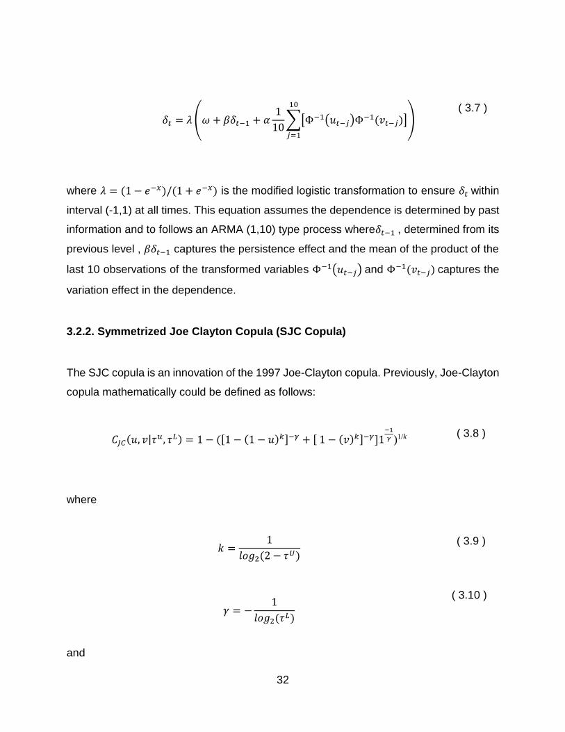
where 𝜆 = (1 − 𝑒−𝑥)/(1 + 𝑒−𝑥) is the modified logistic transformation to ensure 𝛿𝑡 within

interval (-1,1) at all times. This equation assumes the dependence is determined by past

information and to follows an ARMA (1,10) type process where𝛿𝑡−1 , determined from its

previous level , 𝛽𝛿𝑡−1 captures the persistence effect and the mean of the product of the

last 10 observations of the transformed variables Φ−1(𝑢𝑡−𝑗) and Φ−1(𝑣𝑡−𝑗) captures the

variation effect in the dependence.

3.2.2. Symmetrized Joe Clayton Copula (SJC Copula)

The SJC copula is an innovation of the 1997 Joe-Clayton copula. Previously, Joe-Clayton

copula mathematically could be defined as follows:

𝐶𝐽𝐶(𝑢, 𝑣|𝜏𝑢, 𝜏𝐿) = 1 − ([1 − (1 − 𝑢)𝑘]−𝛾 + [ 1 − (𝑣)𝑘]−𝛾]1

−1

𝛾 )1/k ( 3.8 )

where

𝑘 =1

𝑙𝑜𝑔2(2 − 𝜏𝑈)

𝛾 = −1

𝑙𝑜𝑔2(𝜏𝐿)

( 3.9 )

( 3.10 )

and

33

𝜏𝑈𝜖( 0 ,1 ), 𝜏𝐿𝜖 (0 , 1 ). ( 3.11 )

SJC has the characteristic of symmetric when 𝜏 U = 𝜏 L makes it more attractive than the

original Joe–Clayton copula. This characteristic makes the SJC copula have the ability to

capture the lower and upper tail dependence simultaneously. Therefore, this copula is

able to meet the research objectives and help us to understand the tail behaviour of the

data.

Based on the extended version of copula theory (Patton 2006a), SJC can be denoted as:

𝐶𝑆𝐽𝐶(𝑢, 𝑣|𝜏𝑈 , 𝜏𝐿) = 0.5[𝐶𝐽𝐶(𝑢, 𝑣|𝜏

𝑈, 𝜏𝐿) + 𝐶𝐽𝐶(1 − 𝑢, 1 − 𝑣|𝜏𝑈 , 𝜏𝐿) + 𝑢 + 𝑣 − 1] ( 3.12 )

where 𝐶𝐽𝐶 is the Joe–Clayton copula and 𝜏𝑈 and 𝜏𝐿 represent upper and lower tail

dependence.

Mathematically, the evolution parameters for the SJC copula which be used to capture

the dynamic of the upper and lower tail dependences can be denoted in the following

way:

𝜏𝑈/𝐿 = �̃� (𝜔𝑈/𝐿 + 𝛽𝑈/𝐿𝜏𝑡−1 + 𝛼𝑈/𝐿

1

10∑ |𝑢1,𝑡−𝑖 − 𝑢2,𝑡−𝑖|

10

𝑖=1)

( 3.13 )

where �̃� is given as the logistic transformation: �̃�(𝑥) = (1 + 𝑒−𝑥)−1, to ensure the

dependence parameter 𝜏𝑈/𝐿 in interval of (0,1).

34

3.3. Summary

We have outlined the fundamental aspects of EVT and copula in this chapter. The BMM

method will be used in Chapter 4 to identify the best distributions that fit with minima and

maxima series for the Chinese stock market.

The POT and copula method will be used to explain the dependence structure in the

Chinese stock market. More details of research methodology regarding this can be found

in Chapter 5 and Chapter 6, respectively.

35

CHAPTER 4: MODELING THE

DISTRIBUTION OF EXTREME RETURNS

IN THE CHINESE STOCK MARKET

It is well known that extreme share returns on stock markets can have important

implications for financial risk management. In this paper, we are concerned with the

distribution of the extreme daily returns of the Shanghai Stock Exchange (SSE)

Composite Index. Three well-known distributions in extreme value theory, i.e.,

Generalized Extreme Value (GEV), Generalized Logistic (GL) and Generalized Pareto

distributions, are employed to model the SSE Composite index returns based on the data

from 1991 to 2013. The parameters for each distribution are estimated by using the Power

Weighted Method (PWM). Our results indicate that the GL distribution is a better fit for the

minima series and that the GEV distribution is a better fit for the maxima series of the

returns for the Chinese stock market. This is in contrast to the findings for other markets,

such as the US and Singapore markets. Our results are robust regardless of the

introduction of stock movement restriction and the global financial crisis. Further, the

implications of our findings for risk management are discussed.

Keywords: Chinese stock market, extreme value theory, extreme returns, risk

management

This chapter is reproduced from a paper published in Journal of International Financial Markets, Institutions & Money. This chapter

has its reference section and style according to this journal’s requirements. To accommodate with the thesis structure, figure numbers

have been changed and differ from the published version.

36

4.1. Introduction and Literature Review

Extreme movements in share returns rarely occur. However, they can have devastating

consequences when they do occur. Thus, it is important for investors, speculators and

risk managers to comprehend extreme market movement events. Modeling the

distribution of extreme stock returns has become a hot research topic, and it can

contribute to the improvement in risk management.

In the finance literature, it is common to assume that the stock returns follow a Gaussian

distribution. For example, Markowitz (1952) and Sharpe (1964) assume normality of the

distribution for the stock returns in studying portfolio selection and deriving the capital

asset pricing model; Black and Myron (1973) and Merton (1973) assume that the stock

price follows the geometric Brownian motion in their option pricing model. More recently,

Value at Risk (VaR) models developed and implemented by financial institutions also rely

heavily on the Gaussian distribution.

The normality assumption implies that the stock return distribution is symmetric, which

may not be true for right-skewed or left-skewed financial data. Previous studies including

Longin (1996), Jondeau and Rockinger (2003), Tolikas and Gettinby (2009) have

indicated that this assumption may lead to the underestimation of risk. It has been widely

accepted that stock returns tend to be fat tailed rather than normally distributed. Thus, the

normal distribution assumption is often inadequate in accounting for the catastrophic

events and must be dropped for modeling the extreme stock returns.

The extreme value theory (EVT) is appealing for modeling the distribution of extreme

stock returns because it focuses only on the extreme returns rather than all returns. EVT

is a study on the distribution of extreme values of a random variable, and it has been

applied widely in many fields such as hydrology, insurance and finance. It was first

introduced by Fisher and Tippett (1928) and applied by Longin (1996), Embrechts et al.

(1999) and Poon et al. (2004) in finance.

37

EVT is used to model the distribution of stock returns by specifically focusing on the tails.

Parkinson (1980) reveals that the tail of the empirical distribution contains important

information for the variance of returns. The fatness of the tails of the return distribution

can be used to calculate the probabilities of a market crash and thus can contribute to the

early warning of market risk (Jansen and De Vries, 1991). EVT is also used to the

calculation of VaR. Further details can be seen in Cotter (2007), Allen et al. (2013),

Marimoutou et al. (2009) and Karmakar (2013). These studies use the Peak Over

Threshold (POT) method to model the extreme behavior in financial markets. The POT

method considers the sorting of clustered phenomena that are frequently found in data.

In contrast, there has been a decline in the number of studies of EVT by using the Block

Maxima Minima (BMM) method, which defines extreme events as the maximum

(minimum) value in each sub-period.

This research is concerned with the Chinese stock market and aims to identify the best

distribution in modeling extreme stock returns by using the BMM method. The main

distributions assigned to BMM are the Generalized Extreme Value (GEV), Generalized

Logistic (GL) and Generalized Pareto (GP). Studies by Longin (1996), Jondeau and

Rockinger (2003) and Gencay and Selcuk (2004) find that extreme stock returns in the

US can be characterized by the GEV distribution, which can be used for calculating VaR

measures and capital requirements. Gettinby et al. (2004 & 2006) find Generalized

Logistic (GL) distribution fits better for extreme daily share return in the US, UK and Japan

compared to GEV, in contrast to the previous research. More recently, Tolikas and

Gettinby (2009) find that GL distribution is the best fit for the distribution of the extreme

daily share returns in Singapore. In sum, the literature confirms that the best distribution

for extreme share returns varies across share markets. This may be due to the economic

environment and market mechanism of each market. Thus, it is of particular interest to

consider the emerging markets such as the Chinese stock market.

This research aims to fill the gap in the literature by modeling the extreme stock returns

in the Chinese stock market. Due to the similarity between the Shanghai Stock Exchange

(SSE) and Shenzhen Stock Exchange (SZSE), we focus on the SSE Composite Index,

which consists of 950 stocks listed on the SSE.

38

Using the data of Shanghai Stock Exchange Composite Index (SSE Composite) from

1991 to 2013 (23 years), we model the extreme share daily returns of the SSE composite

index by employing an EVT approach. Based on the literature review, we focus on the

Generalized Pareto (GP), Generalized Extreme Value (GEV) and Generalized Logistic

(GL). The parameters of each distribution are estimated by using the Probability Weighted

Moments (PWM) method. Our research reveals that the GL distribution fits the empirical

data better than the GEV and GP distribution for most intervals in minima series, while

GEV distribution fits better for the maxima series of the returns for all intervals.

As a robustness check, we consider two important events during the period: the

introduction of the restriction on the stock movement in Chinese stock market and the

global financial crisis (GFC) of 2007-2008. For each event, we consider the pre- and post-

event periods. It is demonstrated that there is no change in terms of the best distribution

due to these events, though the GFC does have an impact with respect to the best

distribution of the extreme stock returns during the GFC period.

Our findings have important implications for VaR calculation, risk managers, speculators

and risk policies in understanding the distribution of extreme stock returns in the Chinese

stock market.

The remainder of this paper is organized as follows. A background on the Chinese stock

market is provided in Section 4.2. Section 4.3 describes the data and sample statistics.

The research methodology is discussed in Section 4.4. Specifically, we discuss block

maxima sampling, L-moment ratio diagram, parameters estimation and the goodness of

fit test. Section 4.5 presents the empirical results. Section 4.6 discusses the implications

of the findings for the Chinese stock market. A summary and concluding remarks are

given in Section 4.7.

39

4.2. The Chinese Stock Market

The Chinese stock market has grown enormously in the past two decades due to its

miraculous economic development, and it has become more and more influential among

world stock markets. In terms of capitalization, the Chinese stock market has surpassed

Japan and become the second largest stock market behind the US stock market since

the end of 2007. There are two main stock exchanges in China, namely, the Shanghai

Stock Exchange (SSE) and Shenzhen Stock Exchange (SZSE). Both stock exchanges

started trading in 1990. At the end of 2010, the total market capitalization for the Shanghai

Stock Exchange was approximately 18,238 billion RMB with 901 listed companies

(Chong et al., 2012).

The Chinese stock market is an emerging market with many interesting features. There

are two types of shares in the Chinese stock market: A Shares and B Shares. A shares

are restricted to domestic investors only, and B shares are available to both domestic and

foreign investors. Initially, B Shares were stocks that were designated for foreign investors

that were denominated in the Chinese local currency, the Renminbi (RMB), and were

payable in foreign currency. However, the regulation changed in 2001; domestic traders

can now trade B shares in US dollars as well. When the regulation was introduced, a

great deal of B share prices went up significantly (Chen et al., 2007).

It is worth noting that there is a limit of 10 percent in the daily movement in share price

since 16 December 1996 to curb excessive volatility. An additional important feature is

that 70 percent of shares are non-tradable, held by the government, state-owned

enterprises (SOEs) and Chinese institutions (Mookerjee and Yu, 1999). Thus, the

Chinese government may have more influence on the Chinese stock market compared

to developed markets such as the US and the UK.

Apart from restrictions on the daily movement and ownership, there are two other features

in the Chinese stock market that can have a significant impact on the share price

movement. First, short-sale trading is strictly prohibited in the Chinese stock market. This

characteristic limits the supply of shares and affects the stock price formation. Second,

40

unlike developed markets, the major market participants in the Chinese stock market are

individual investors. The number of A-share individual accounts is 57.59 million, which is

in contrast to the 1.35 million accounts owned by institutional investors at the end of

20004. Thus, there are a huge number of unsophisticated individual investors in the

market. With the low transparency in the market and the lack of qualified security analysts,

individual investors can behave like noise traders, and they often trade on rumors and

past price trends (Kang et al., 2002). With the short-sale prohibition, trading volume is

likely to indicate the sentiment of these irrational investors.

The above-mentioned features make the study on the Chinese stock market interesting

and challenging. The Chinese stock market has thus been extensively studied in the

finance literature in recent years. For example, Xu (2000) studies the microstructure of

the Chinese stock market; few studies, including Eun and Huang (2007) and Chan et al.

(2006), consider the asset pricing in the Chinese stock market; Los and Yu (2008) and

Zhu (2006) study the stock price and return properties in the Chinese stock market; the

anomalies in the Chinese stock market are considered in Mookerjee and Yu (1999), and

Naughton et al. (2008) study the trading strategies based on A- and B-share market

segmentation.

Though there are many studies on the Chinese stock market in the literature, there is

limited understanding of the behavior of its extreme stock returns. Recent studies in EVT

demonstrate the need for understanding the financial market, especially during a financial

crisis. Many studies so far focus on the developed stock markets including the United

States (US), United Kingdom (UK) and Japan. To the best of our knowledge, no study

has been performed in the Chinese market based on EVT. This study aims to fill this gap.

In this research, we also study the effect of the price restriction on the distributions of

extreme returns in the Chinese stock market. The price restriction on the Chinese stock

market was initially in force when the stock exchange started trading in 1990. The

restriction was imposed on daily aggregate price fluctuations of the Shanghai stock

4 Source, the websites of SSE and SZSE: www.sse.com.cn and www.sse.org.cn

http://www.sse.com.cn/

http://www.sse.org.cn/

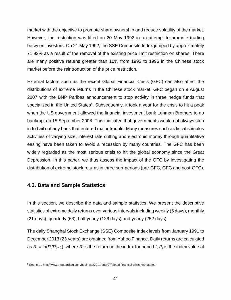
41

market with the objective to promote share ownership and reduce volatility of the market.

However, the restriction was lifted on 20 May 1992 in an attempt to promote trading

between investors. On 21 May 1992, the SSE Composite Index jumped by approximately

71.92% as a result of the removal of the existing price limit restriction on shares. There

are many positive returns greater than 10% from 1992 to 1996 in the Chinese stock

market before the reintroduction of the price restriction.

External factors such as the recent Global Financial Crisis (GFC) can also affect the

distributions of extreme returns in the Chinese stock market. GFC began on 9 August

2007 with the BNP Paribas announcement to stop activity in three hedge funds that

specialized in the United States5. Subsequently, it took a year for the crisis to hit a peak

when the US government allowed the financial investment bank Lehman Brothers to go

bankrupt on 15 September 2008. This indicated that governments would not always step

in to bail out any bank that entered major trouble. Many measures such as fiscal stimulus

activities of varying size, interest rate cutting and electronic money through quantitative

easing have been taken to avoid a recession by many countries. The GFC has been

widely regarded as the most serious crisis to hit the global economy since the Great

Depression. In this paper, we thus assess the impact of the GFC by investigating the

distribution of extreme stock returns in three sub-periods (pre-GFC, GFC and post-GFC).

4.3. Data and Sample Statistics

In this section, we describe the data and sample statistics. We present the descriptive

statistics of extreme daily returns over various intervals including weekly (5 days), monthly

(21 days), quarterly (63), half yearly (126 days) and yearly (252 days).

The daily Shanghai Stock Exchange (SSE) Composite Index levels from January 1991 to

December 2013 (23 years) are obtained from Yahoo Finance. Daily returns are calculated

as Rt = ln(Pt/Pt − 1), where Rt is the return on the index for period t, Pt is the index value at

5 See, e.g., http://www.theguardian.com/business/2011/aug/07/global-financial-crisis-key-stages.

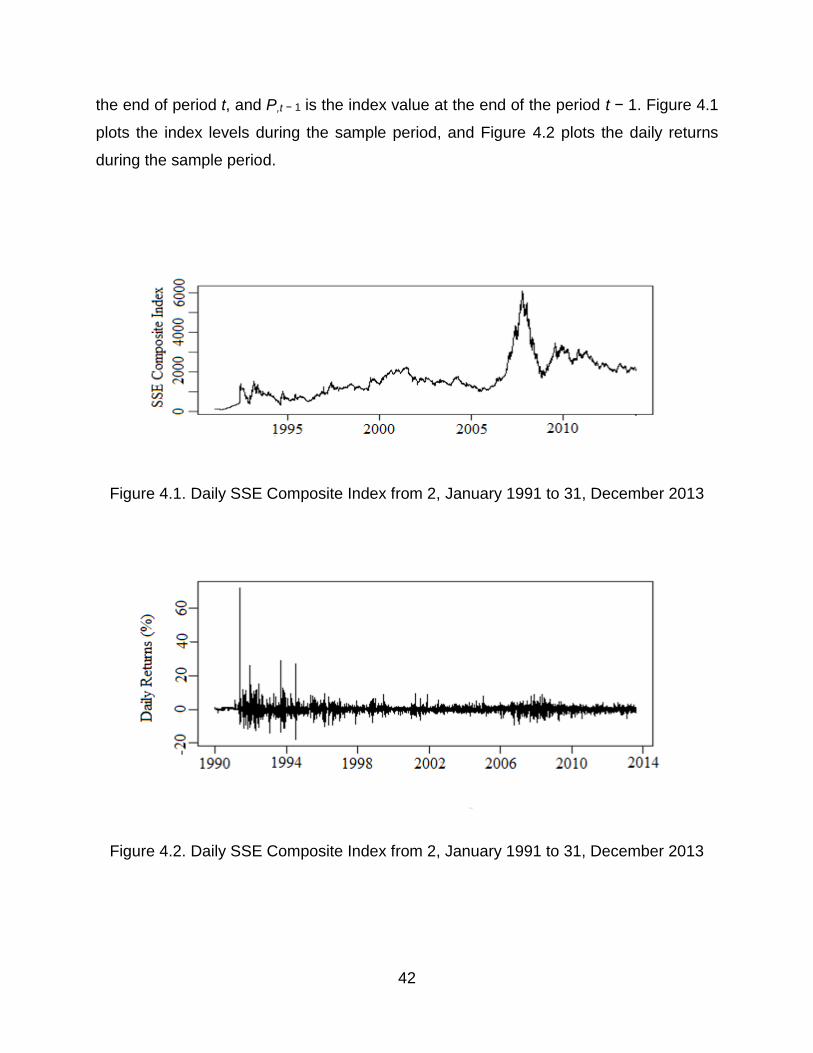
42

the end of period t, and P,t − 1 is the index value at the end of the period t − 1. Figure 4.1

plots the index levels during the sample period, and Figure 4.2 plots the daily returns

during the sample period.

Figure 4.1. Daily SSE Composite Index from 2, January 1991 to 31, December 2013

Figure 4.2. Daily SSE Composite Index from 2, January 1991 to 31, December 2013

43

Figure 4.1 indicates that the SSE composite index had a huge movement during 2007-

2009, in which period the index climbed over 6000 points before it dropped to 2000 as a

consequence of the global financial crisis, which led to stock market crashes worldwide.

Figure 4.2 indicates that the daily log returns remain between -10% and 10% after the

price movement limit was reintroduced in 1996. The volatility of the SSE Composite Index

is much higher during the 1992-1994 period.

It is worth mentioning that Figures 4.1 and 4.2 do not indicate extreme index and index

return movements during the Asian financial crisis period (1997-98). This observation is

consistent with the fact that the Asian financial crisis did not have a substantial impact on

the Chinese economy, as claimed by Mitchell and Ong (2006).

Figure 4.3 displays the QQ plot of the daily log return against the normal distributions.

Much of the data depart from the normal line for the lower and upper tails. This pattern

indicates the existence of the fat tail phenomenon in the SSE Composite Index data. This

justifies the use of the EVT to model the tail distributions.

Figure 4.3. QQ plot of daily log returns against the normal distribution

44

Table 4.1 reports the descriptive statistics for daily index returns as well as the maximum

and minimum series for each interval (weekly, Monthly, Quarterly, Half-Yearly and

Yearly).

A few observations can be made regarding the daily index return series. The lowest daily

return is −17.9051%, and the highest daily return is 28.8610%. The mean is slightly

positive, which indicates an upward movement in the share price. The average standard

deviation is 2.1834%. The skewness for the whole period is 1.2065. The value of kurtosis

is relatively high at 21.3223. These values indicate the non-normality of the distribution.

Further, the Jarque-Bera (JB) test confirms the fat tail and non-normality of the

distribution.

Similar observations regarding the distributions for the minima and maxima for each

series can be made as follows. The average of the minima series is negative for all

intervals. As expected, the value of minima returns decrease as the interval increases.

The standard deviation of the minima series is between two to four for all intervals, which

indicates the volatility are not too far apart from each other compared to the maxima

series. The kurtosis of the minima for the weekly series is much higher compared to the

other intervals. This indicates that the non-normality and fat tail of the minima series for

the weekly interval are more evident than others. A similar pattern holds for the maxima

series for each interval. The average of the maxima series is positive for all intervals. The

lowest value for the standard deviation in the maxima series is 2.4137%, while the highest

is 7.8544%.

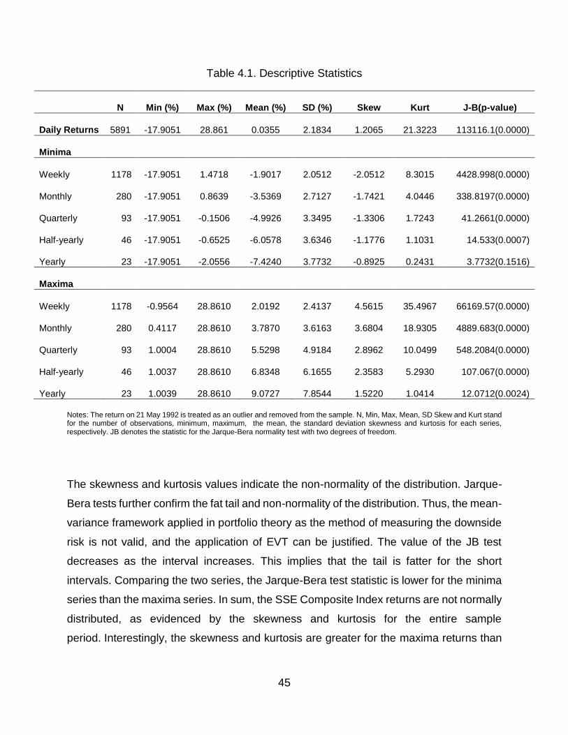
45

Table 4.1. Descriptive Statistics

N Min (%) Max (%) Mean (%) SD (%) Skew Kurt J-B(p-value)

Daily Returns 5891 -17.9051 28.861 0.0355 2.1834 1.2065 21.3223 113116.1(0.0000)

Minima

Weekly 1178 -17.9051 1.4718 -1.9017 2.0512 -2.0512 8.3015 4428.998(0.0000)

Monthly 280 -17.9051 0.8639 -3.5369 2.7127 -1.7421 4.0446 338.8197(0.0000)

Quarterly 93 -17.9051 -0.1506 -4.9926 3.3495 -1.3306 1.7243 41.2661(0.0000)

Half-yearly 46 -17.9051 -0.6525 -6.0578 3.6346 -1.1776 1.1031 14.533(0.0007)

Yearly 23 -17.9051 -2.0556 -7.4240 3.7732 -0.8925 0.2431 3.7732(0.1516)

Maxima

Weekly 1178 -0.9564 28.8610 2.0192 2.4137 4.5615 35.4967 66169.57(0.0000)

Monthly 280 0.4117 28.8610 3.7870 3.6163 3.6804 18.9305 4889.683(0.0000)

Quarterly 93 1.0004 28.8610 5.5298 4.9184 2.8962 10.0499 548.2084(0.0000)

Half-yearly 46 1.0037 28.8610 6.8348 6.1655 2.3583 5.2930 107.067(0.0000)

Yearly 23 1.0039 28.8610 9.0727 7.8544 1.5220 1.0414 12.0712(0.0024)

Notes: The return on 21 May 1992 is treated as an outlier and removed from the sample. N, Min, Max, Mean, SD Skew and Kurt stand for the number of observations, minimum, maximum, the mean, the standard deviation skewness and kurtosis for each series, respectively. JB denotes the statistic for the Jarque-Bera normality test with two degrees of freedom.

The skewness and kurtosis values indicate the non-normality of the distribution. Jarque-

Bera tests further confirm the fat tail and non-normality of the distribution. Thus, the mean-

variance framework applied in portfolio theory as the method of measuring the downside

risk is not valid, and the application of EVT can be justified. The value of the JB test

decreases as the interval increases. This implies that the tail is fatter for the short

intervals. Comparing the two series, the Jarque-Bera test statistic is lower for the minima

series than the maxima series. In sum, the SSE Composite Index returns are not normally

distributed, as evidenced by the skewness and kurtosis for the entire sample

period. Interestingly, the skewness and kurtosis are greater for the maxima returns than

46

for the minima series. This indicates that the upper tail is likely fatter than the lower tail.

This may be due to the existing of many extreme positive returns.

To investigate the impact of the reintroduction of stock movement restriction, we consider

two subsamples: May 1992- Dec 1996 without price restriction and Dec 1996 – Dec 2001

with price restriction. The results are reported in Section 4.5.2.

Similarly, to consider the impact of GFC on the Chinese stock market, we consider the

following three subsamples: Jan. 2002 to Aug. 2007 as the pre-GFC period, Jan. 2007 to

Dec. 2010 as the GFC period6, and Apr. 2009 to Dec. 2013 as the post-GFC period.

6 Due to the fact that we need a sufficient number of observations for the estimates and the follow-on events of the GFC such as the

European debt crisis in 2010, the GFC period is taken until Dec. 2010 instead of Apr. 2009.

47

4.4. Methodology

In this section, we outline the methodology for applying the EVT to model the extreme

stock returns in the Chinese stock market. We first describe the GEV and GL distributions,

which are commonly used for EVT. Then, we introduce the L-Moment ratio diagram for

identifying a suitable extreme distribution. The parameter estimation and the goodness of

fit test are also discussed.

4.4.1. GEV and GL Distribution

Extreme events can be modeled either by the BMM method or the POT method. Because

we are interested in studying the extreme movement in the selected sub-periods, BMM

is suitable for this research.

The intervals in our consideration are the weekly, monthly, quarterly, half-yearly and

yearly minima and maxima. These minima and maxima daily returns are collected over

non-overlapping successive selection intervals of 5 days (weekly), 21 days (monthly),

63 days (quarterly), 126 days (semester) and 252 days (yearly). Given the time series of

daily index returns r1, r2, r3…rn, the series can be divided into non-overlapping time

intervals of length m. The time series of the extreme maximum will then be

X1=max(r1,…,rm), X2=max(rm+1,...,r2m), ..., Xn/m=max(rn-m,...,rn). According to Fisher and

Tippett (1928), the distribution of the extreme series is best fitted with the GEV, which is

assumed to be independent and identical. GEV is known as a three-parameter distribution

defined as:

𝑓(𝑥) = 𝛼−1𝑒−(1−𝐾)𝑦𝑒−𝑒−𝑦, where 𝑦 = {

−𝐾−1𝑙𝑜𝑔{1 − 𝐾(𝑥 − 𝛽)/𝛼},𝐾 ≠ 0(𝑥 − 𝛽)/𝛼, 𝐾 = 0

( 4.1 )

The parameters are referred to as the location (β), scale (α) and shape (κ). The location

parameter (β) is analogous to the mean and the scale (α) parameter is analogous to the

48

standard deviation. The shape parameter (κ) determines the fatness of the tail of the

distribution. The larger the value of shape parameter (κ), the fatter the tail is.

According to Peel et al. (2001), this 3-parameter distribution is particularly effective in

describing the probability distributions of extreme events in environmental studies.

Further, a few special cases of the GEV distribution are worth mentioning. The

Frechet distribution is obtained when β+α/K < x ≤ ∞, where K<0. Known as the reverse of

GEV, the Weibull distribution is obtained when K > 0 with -∞ < x ≤ β+α. The Gumbel

distribution is obtained when K=0 with -∞ < x < ∞.

There is strong evidence that autocorrelation and heteroskedasticity persist in the

financial data. With most stock market index returns, GL distribution appears to be a better

fit than GEV distribution for extreme returns (Tolikas, 2008). The GL function is given as:

𝑓(𝑥) = 𝛼−1𝑒−(1−𝐾)𝑦/(1 + 𝑒−𝑦)2, where 𝑦 = {−𝐾−1𝑙𝑜𝑔{1 − 𝐾(𝑥 − 𝛽)/𝛼}, 𝐾 ≠ 0(𝑥 − 𝛽)/𝛼, 𝐾 = 0

( 4.2)

The logistic distribution is obtained when K = 0 for -∞ < x < ∞, when K < 0 for β+α/K < x ≤

∞ and when K > 0 for -∞ < x ≤ β+α .

4.4.2. L-Moment Ratio Diagram

To select a probability distribution for a set of empirical data, we apply the L-moment ratio

diagram, which is a graphical test introduced by Hosking (1990). The diagram involves

five distributions: Generalized Extreme Value (GEV), Generalized Pareto (GP),

Generalized Logistic (GL), Gumbel (G) and Normal (N).

The L-moment, λ r for a random variable X is defined as:

𝜆𝑟 = 𝑟−1∑(−1)𝑘

𝑟−1

𝐾=0

(𝑟 − 1

𝐾)𝐸𝑋(𝑟−𝑘:𝑟), 𝑟 = 1, 2…

( 4.3 )

49

where 𝐸𝑋(𝑟−𝑘:𝑟) is the expectation of the (𝑟 − 𝑘)𝑡ℎ extreme order statistic. The first two

moments, λ 1 and λ 2, are measures of location and scale. The L-moment ratios, Ƭ3 = λ 1/λ

2 and Ƭ 4 = λ 2/λ 2, are measures of skewness and kurtosis, respectively.

The values of the L-moment ratios for common continuous probability distributions are

normally constant. For example, the value of Ƭ 3 is 0.1226, while the value of Ƭ 4 is 0 for a

normal distribution. However, for more complex distributions including GEV, GL: and GP,

L-moment ratios are not constant.

In the L-moment ratio diagram, L-kurtosis values are plotted against the L-skewness

values. The diagram contains the points and curves of the theoretical distributions. The

best distribution for the data is identified by plotting the estimated Ƭ3 and Ƭ4 and choosing

the distribution for which the L-skewness and L-kurtosis theoretical curve is closest to the

plotted point.

4.4.3. The Parameter Estimation

It is common to use the maximum likelihood (ML) method to estimate the parameters of

a distribution. However, Tolikas (2008) and Gettinby et al. (2004) suggest the use of

probability weighted moments (PWM) to estimate parameters for GEV, GL and GP in

modeling the extreme returns of financial series.

PWM is the expectation of certain functions of a random variable X with distribution

function F, the mean of which exists and its distribution can be written in inverse form.

According to Hosking (1986), PWM can be defined as:

∝𝑟= 𝐸[𝑋{1 − 𝐹(𝑋)}]𝑟 , 𝑟 = 0,1… ( 4.4 )

where 𝐸[𝑋(… . )] is the expectation of the quartile function of a random variable X. The

PWM method estimates the parameters of a distribution by equating the sample moments

to those of the fitted distribution.

50

Compared to the ML method in parameter estimation, the PWM method can yield a lower

root mean-square error. More specifically, the PWM method is able to obtain less biased

parameter and quantile estimates. In addition, this approach has the ability to minimize

sampling error for the parameter estimate compare to ML. The estimation of parameters

and quantiles by the PWM method are found to be much more efficient for GEV

distribution than those estimated by the ML method (Hosking et al. (1985), Hosking and

Wallis (1987) and Moharram et al. (1993)).

4.4.4. The Goodness of Fit Measure

After a distribution is fitted to the empirical data, it is important to test the goodness of fit

of the chosen distribution. There are many goodness of fit tests. In this paper, we consider

Anderson Darling Test (AD), which is described below.

4.4.4.1. Anderson Darling (AD) Test

The Anderson Darling test is the modified version of the Cramer-von Mises (CvM) test.

This test yields better results compared to the CvM, test as it gives more weight to the

tails of the distribution. According to Arshad et al. (2003), the AD test is the most powerful

tool for the empirical distribution function (EDF) test. Much of the time, it performs better

than the Kolmogorov Smirnov test in terms of power statistical comparisons. Thus, we

choose the AD test for the goodness of the fit test in the paper.

The test statistic for Anderson Darling is defined as:

∫ [𝐹𝑛∞

−∞(𝑥) − 𝐹(𝑥)]2∅(𝑥)𝑑𝐹(𝑥) ( 4.5 )

where 𝐹𝑛(𝑥) denotes the empirical distribution function (EDF) of a random

variable X, 𝐹(𝑥) is the cumulative distribution function (CDF) of X, n denotes the number

of observations and ∅(𝑥) is a function that assigns weight to the squared difference

[Fn(x) − F(x)]2.

51

When ∅(𝑥) = [𝐹(𝑥)(1 − 𝐹(𝑥) )]−1, the test statistic concentrates on calculating

discrepancies in both tails; if either 𝐹(𝑥) or [1 − 𝐹(𝑥)] is small or ∅(𝑥) is large.

According D'Agostino and Stephens (1986), the Anderson-Darling (AD) goodness of fit

test can be more effective in a small sample than the Pearson chi-squared test. The lower

the value for the AD test statistic, the better is the fit for the empirical data.

4.5. Empirical Results

In this section, we present the empirical results. We first discuss the L-moment ratio

diagrams and then present and analyse the results on the parameter estimation for the

GEV and GL distributions and goodness of fit tests.

Figures 4.4 and 4.5 present the L-moment ratio diagrams for the minima and maxima

series, respectively. For each series, the L-skewness and L-kurtosis are calculated and

plotted on the graph, with each point representing one of the five intervals of weekly,

monthly, quarterly, half-yearly and yearly. In addition, the L-moment ratio curves for

Generalized Logistic, Generalized Extreme Value, Generalize Pareto, Gumbel and

Normal distributions are also plotted.

For the minima series, Figure 4.4 indicates that the L-moment ratios for the five intervals

are between the L-moment ratio curves for the GL and GEV distributions. For the 4.5

maxima, Figure 4.5 indicates that the L-moment ratios for the 5 intervals are very close

to the L-moment ratio curves for the GL and GEV distributions. Hence, the Normal,

Gumbel and GP distributions can be eliminated from further consideration.

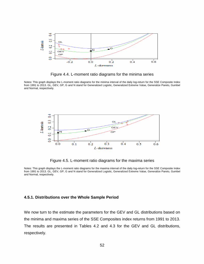
http://www.sciencedirect.com/science/article/pii/S0927539808000558#bib4

52

Figure 4.4. L-moment ratio diagrams for the minima series

Notes: This graph displays the L-moment ratio diagrams for the minima interval of the daily log-return for the SSE Composite Index from 1991 to 2013. GL, GEV, GP, G and N stand for Generalized Logistic, Generalized Extreme Value, Generalize Pareto, Gumbel and Normal, respectively.

Figure 4.5. L-moment ratio diagrams for the maxima series

Notes: This graph displays the L-moment ratio diagrams for the maxima interval of the daily log-return for the SSE Composite Index from 1991 to 2013. GL, GEV, GP, G and N stand for Generalized Logistic, Generalized Extreme Value, Generalize Pareto, Gumbel and Normal, respectively.

4.5.1. Distributions over the Whole Sample Period

We now turn to the estimate the parameters for the GEV and GL distributions based on

the minima and maxima series of the SSE Composites index returns from 1991 to 2013.

The results are presented in Tables 4.2 and 4.3 for the GEV and GL distributions,

respectively.

53

Table 4.2. Parameter estimates for GEV distribution

Shape Scale Location AD p-value

Minima

Weekly -0.9318 2.0168 -1.9601 185.5800 0.0042

Monthly -0.9197 2.7793 -3.6316 43.1170 0.0806

Quarterly -0.8761 3.5701 -5.1808 15.6220 0.4053

Half-yearly -0.8212 3.9491 -6.3599 4.1023 0.9356

Yearly -0.7055 4.3560 -7.9817 0.1346 0.9639

Maxima

Weekly* 0.1795 1.2841 0.8252 18.5270 0.0001

Monthly* 0.3587 1.3978 2.2222 0.3116 0.9438

Quarterly* 0.3201 2.1205 3.3369 0.2003 0.9820

Half-yearly 0.3667 2.4770 4.0144 0.3983 0.7707

Yearly* 0.3633 3.4686 5.1518 0.4422 0.7815

Notes: This table displays the parameter estimates and goodness of fit figures for the GEV distribution for the minima and maxima series of the 5 intervals over the sample period. AD denotes the Anderson-Darling test. p-value denotes the probability of such a fit being obtained in a random sample from a GEV distribution. * means the considered distribution is a better fit than the other one based on the AD test.

54

Table 4.3. Parameter estimates for GL distribution

Shape Scale Location AD p-value

Minima

Weekly* -0.3067 0.8541 -1.4192 4.9256 0.2444

Monthly* -0.3019 1.1821 -2.8819 0.8818 0.4107

Quarterly* -0.2842 1.5432 -4.1979 0.7041 0.3301

Half-yearly* -0.2614 1.7435 -5.2447 0.3565 0.7401

Yearly* -0.2111 2.0166 -6.6861 0.1318 0.9854

Maxima

Weekly 0.2906 0.9382 1.3445 50.2700 0.0015

Monthly 0.4223 1.1276 2.8065 0.4645 0.9024

Quarterly 0.3929 1.6749 4.2181 0.2307 0.9184

Half-yearly* 0.4285 2.0069 5.0510 0.3815 0.8276

Yearly 0.4259 2.8050 6.6027 0.4563 0.7895

Notes: This table displays the parameter estimates and goodness of fit figures for the GL distribution for the minima and maxima series of the 5 intervals over the sample period. AD denotes the Anderson-Darling test. p-value denotes the probability of such a fit being obtained in a random sample from a GL distribution. * means the considered distribution is a better fit than the other one based on the AD test.

The shape parameter estimates for the Chinese stock market reveal some interesting

facts. For example, the shape parameter estimates for the minima series for GEV

distribution increases from -0.9318 for Weekly to -0.7055 for the Yearly interval. For the

maxima series, the shape parameter estimate increases as the time interval increases.

Hence, the tails for both distributions become fatter for larger intervals. Similar

observations can be observed for the GL distribution from Table 4.3.

It is known that the scale parameter is related to the volatility. For GEV distribution, the

scale parameter estimate increases from 2.0168 to 4.3560 for the minima series and

1.2841 to 3.4686 for the maxima series as the interval increases from Weekly to Yearly.

For GL distribution, we can see that the scale parameter estimates increase from 0.8541

55

to 2.0166 for the minima series and 0.8166 to 2.9719 for the maxima series as the interval

increases from Weekly to Yearly. This is consistent with the intuition that extreme daily

returns are more volatile for a longer period of the time interval.

Based on the AD statistics in Tables 4.2 and 4.3, we can find the better fit distribution

among GEV with the GL for each series. Our results indicate that GL distribution fits better

than GEV distribution for the minima series for all five intervals. However, GEV fits better

for the maxima series for all intervals except the Half-yearly interval. Overall, we can

claim that GEV fits the maxima series better, while GL is a better fit for the minima series.

4.5.2. The Impact of Stock Movement Restriction

As the robustness check of our results, we here consider the impact due to the

introduction of the stock movement restriction in 1996. The above analysis for the whole

sample period is thus carried out for two sub-periods: May 1992 to Dec 1996 without the

10 percent daily movement restriction and Dec. 1996 to Dec. 2001 with the 10 percent

daily movement restriction. The results are reported in Table 4.4 for GEV and in Table

4.5 for GL. Note that due to the limited number of observations for each sub-period, we

present the results only for three time intervals, i.e., Weekly, Monthly and Quarterly.

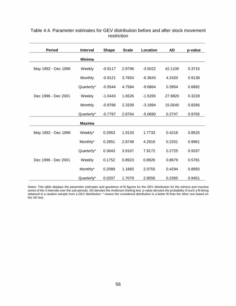
56

Table 4.4. Parameter estimates for GEV distribution before and after stock movement restriction

Period Interval Shape Scale Location AD p-value

Minima

May 1992 - Dec 1996 Weekly -0.9117 2.9796 -3.5022 42.1100 0.3715

Monthly -0.9121 3.7654 -6.3643 4.2420 0.9138

Quarterly* -0.5544 4.7584 -9.6864 0.3954 0.6892

Dec 1996 - Dec 2001 Weekly -1.0443 1.6526 -1.5265 27.9820 0.3228

Monthly -0.9786 2.3339 -3.1894 15.0540 0.8266

Quarterly* -0.7797 2.8764 -5.0690 0.2747 0.9765

Maxima

May 1992 - Dec 1996 Weekly* 0.2953 1.9133 1.7733 0.4216 0.8525

Monthly* 0.2851 2.8748 4.2916 0.2201 0.9961

Quarterly* 0.3043 3.9167 7.9172 0.2725 0.9337

Dec 1996 - Dec 2001 Weekly 0.1752 0.8923 0.8926 0.8679 0.5781

Monthly* 0.2089 1.1865 2.0755 0.4294 0.8955

Quarterly* 0.0207 1.7079 2.9556 0.2365 0.9451

Notes: This table displays the parameter estimates and goodness of fit figures for the GEV distribution for the minima and maxima series of the 3 intervals over the sub-periods. AD denotes the Anderson-Darling test. p-value denotes the probability of such a fit being obtained in a random sample from a GEV distribution. * means the considered distribution is a better fit than the other one based on the AD test.

57

Table 4.5. Parameter estimates for GL distribution before and after stock movement restriction


Minima

May 1992 - Dec 1996 Weekly* -0.2987 1.2710 -2.6954 0.5739 0.5731

Monthly* -0.2988 1.6060 -5.3450 0.6221 0.6933

Quarterly -0.1407 2.3565 -8.1773 0.5963 0.4855

Dec 1996 - Dec 2001 Weekly* -0.3501 0.6734 -1.1069 0.6003 0.7585

Monthly* -0.3251 0.9722 -2.5774 0.2556 0.9846

Quarterly* -0.2437 1.2912 -4.2413 0.4227 0.7539

Maxima

May 1992 - Dec 1996 Weekly 0.3744 1.4908 2.5652 0.7094 0.6416

Monthly 0.3668 2.2274 5.4793 0.2636 0.9659

Quarterly 0.3811 3.0670 9.5408 0.2899 0.9345

Dec 1996 - Dec 2001 Weekly* 0.2876 0.6503 1.2531 0.5619 0.6696

Monthly 0.3114 0.8812 2.5584 0.6175 0.7449

Quarterly 0.1833 1.1415 3.6191 0.3008 0.8873

Notes: This table displays the parameter estimates and goodness of fit figures for the GL distribution for the minima and maxima series of the 3 intervals over the sub-periods. AD denotes the Anderson-Darling test. p-value denotes the probability of such a fit being obtained in a random sample from a GL distribution. * means the considered distribution is a better fit than the other one based on the AD test.

According to Tables 4.4 and 4.5, the scale parameter estimates increase as the interval

increases regardless of the sub-periods. This reconfirms the fact that there is a higher

volatility in the stock returns for a longer time interval. Similar observations for the shape

and location parameter estimates can be said as for the whole sample period. The values

of scale parameter are higher before the restriction on the stock market is reintroduced.

This indicates that the volatility of the stock index is higher before stock price movement

restriction reintroduction.

58

However, a comparison of Table 4.4 with Table 4.5 reveals that GL distribution is a better

fit for the minima series for the Weekly and Monthly intervals. For the maxima series,

GEV distribution is a better fit for all intervals except Weekly interval after restriction

reintroduction. Overall, the change of the regulation does not affect the types of

distribution for extreme returns of the SSE index. This can be explained as follows.

First, the 10% restriction on stock market movement appears to be too high for the index

because the average movement for the SSE index is between -1% and 1%. Hence, the

impact of the stock movement restriction is limited on the SSE index. Second, the majority

of the traders or investors in the Chinese stock market are individuals who have limited

resources to swing the market. The selected index consists of for the most part the blue

chip stocks that are hard to manipulate. Thus, the stock price movement restriction of

10% rarely comes into effect for the stocks in the SSE composite index.

In sum, the best-fit distribution results for the whole sample periods hold regardless of the

stock price movement restriction regulation

4.5.3. The Impact of the GFC

In this section, we investigate the impact of the GFC on the Chinese stock market with

respect to the distribution of extreme returns. According to Dungey and Zhumabekova

(2001) and Wen et al.(2012), the test of effect can be seriously affected by the size of the

“crisis” and “non-crisis” period. For this study, three subsamples are considered: Jan.

2002 to Aug. 2007 as the pre-GFC period, Jan. 2007 to Dec. 2010 as the GFC period,

and Apr. 2009 to Dec. 2013 as the post-GFC period. The results are reported in Table

4.6 for GEV and Table 4.7 for GL.

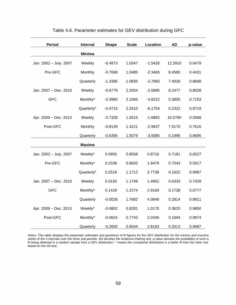
59

Table 4.6. Parameter estimates for GEV distribution during GFC


Minima

Jan. 2002 – July. 2007 Weekly -0.4973 1.0347 -1.5426 12.3910 0.6479

Pre-GFC Monthly -0.7668 1.0485 -2.3465 8.4585 0.4431

Quarterly -1.3395 1.0835 -2.7983 7.4026 0.8848

Jan. 2007 – Dec. 2010 Weekly -0.6779 2.2054 -2.6895 8.2477 0.8028

GFC Monthly* -0.3990 2.1065 -4.8222 0.3855 0.7153

Quarterly* -0.4715 2.2510 -6.1754 0.2322 0.9719

Apr. 2009 – Dec. 2013 Weekly -0.7328 1.2615 -1.6892 16.5760 0.5568

Post-GFC Monthly -0.8139 1.4221 -2.9637 7.9170 0.7616

Quarterly -0.6356 1.5079 -3.9385 0.1995 0.9695

Maxima

Jan. 2002 – July. 2007 Weekly* 0.0950 0.8558 0.8716 0.7181 0.6527

Pre-GFC Monthly* 0.2338 0.8620 1.9479 0.7043 0.5917

Quarterly* 0.2518 1.1712 2.7738 0.1622 0.9987

Jan. 2007 – Dec. 2010 Weekly 0.0150 1.1748 1.4952 0.6333 0.7429

GFC Monthly* 0.1429 1.2274 2.9183 0.1738 0.9777

Quarterly -0.0028 1.7682 4.0848 0.2814 0.8911

Apr. 2009 – Dec. 2013 Weekly* -0.0802 0.8281 1.0170 0.3625 0.9850

Post-GFC Monthly* -0.0624 0.7743 2.0349 0.1694 0.9974

Quarterly -0.2600 0.9044 2.8183 0.2013 0.9687

Notes: This table displays the parameter estimates and goodness of fit figures for the GEV distribution for the minima and maxima series of the 3 intervals over the three sub-periods. AD denotes the Anderson-Darling test. p-value denotes the probability of such a fit being obtained in a random sample from a GEV distribution. * means the considered distribution is a better fit than the other one based on the AD test.

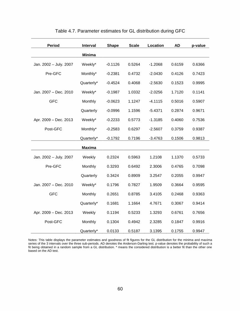
60

Table 4.7. Parameter estimates for GL distribution during GFC


Minima

Jan. 2002 – July. 2007 Weekly* -0.1126 0.5264 -1.2068 0.6159 0.6366

Pre-GFC Monthly* -0.2381 0.4732 -2.0430 0.4126 0.7423

Quarterly* -0.4524 0.4068 -2.5630 0.1523 0.9995

Jan. 2007 – Dec. 2010 Weekly* -0.1987 1.0332 -2.0256 1.7120 0.1141

GFC Monthly -0.0623 1.1247 -4.1115 0.5016 0.5907

Quarterly -0.0996 1.1596 -5.4371 0.2874 0.9671

Apr. 2009 – Dec. 2013 Weekly* -0.2233 0.5773 -1.3185 0.4060 0.7536

Post-GFC Monthly* -0.2583 0.6297 -2.5607 0.3759 0.9387

Quarterly* -0.1792 0.7196 -3.4763 0.1506 0.9813

Maxima

Jan. 2002 – July. 2007 Weekly 0.2324 0.5963 1.2108 1.1370 0.5733

Pre-GFC Monthly 0.3293 0.6492 2.3006 0.4765 0.7098

Quarterly 0.3424 0.8909 3.2547 0.2055 0.9947

Jan. 2007 – Dec. 2010 Weekly* 0.1796 0.7827 1.9509 0.3664 0.9595

GFC Monthly 0.2651 0.8785 3.4105 0.2468 0.9363

Quarterly* 0.1681 1.1664 4.7671 0.3067 0.9414

Apr. 2009 – Dec. 2013 Weekly 0.1194 0.5233 1.3293 0.6761 0.7656

Post-GFC Monthly 0.1304 0.4942 2.3285 0.1847 0.9916

Quarterly* 0.0133 0.5187 3.1395 0.1755 0.9947

Notes: This table displays the parameter estimates and goodness of fit figures for the GL distribution for the minima and maxima series of the 3 intervals over the three sub-periods. AD denotes the Anderson-Darling test. p-value denotes the probability of such a fit being obtained in a random sample from a GL distribution. * means the considered distribution is a better fit than the other one based on the AD test.

61

A few interesting observations can be made from Tables 4.6 and 4.7. First, let us consider

the pre- and post-GFC periods. Similar to Tables 4.4 and 4.5, GL distribution is a better

fit for the minima series for all intervals, and GEV distribution is a better fit for the maxima

series with many of the intervals regardless of the pre- or post-GFC periods. The only

exception is that GL distribution appears to be a better fit for the maxima series for the

Quarterly interval in the post-GFC period. Further, the values of the shape parameter are

negative for the minima series for both pre- and post-GFC periods. This indicates that the

minima series has a fatter tail. The values of the shape parameter for the post-GFC period

are lower than the ones for the pre-GFC period. This implies that the downside risk is

larger before GFC than after GFC. Finally, the values of the scale parameter for the post-

GFC period are similar to the ones for the pre-GFC period. This implies that there is no

long-term impact of GFC on the volatility of the extreme stock returns.

Next, let us consider the GFC period. The best distributions swing between GL and GEV

for different intervals for both the minima series and maxima series during the GFC period.

In other words, there is no single distribution that is consistently better for all time intervals

for either the maxima or minima series. Thus, GFC had a significant impact on the

distribution of extreme stock returns in the Chinese stock market during the GFC period.

Overall, we can claim that there is no long-term change with respect to the best

distributions of extreme stock returns in the Chinese stock market due to the GFC,

although a significant impact is found during the GFC period.

In summary, our empirical results in this section reveal that both GL and GEV are needed

for modeling the extreme stock returns for the Chinese stock market. GL is better at

modeling the downside extreme market movements, while GEV is better at modeling the

upside extreme market movements. It is worth noting that the results for the Chinese

stock market are in stark contrast to the ones for the majority of other markets in the

literature, in which only one distribution (either GL or GV) for each market is found to be

a better fit for both types of extreme market movements. It is also demonstrated that there

is no long-term change with respect to the best distributions of extreme stock returns in

62

the Chinese stock market due to the GFC, although a significant impact is found during

the GFC period.

4.6. Implications for the Chinese Stock Market

The improvement in modeling the distribution of the tails can bring benefits to risk

management. VaR is one of the most widely used models for measuring market risk due

to its simplicity. In essence, VaR tells us how much we can lose over a certain time

horizon with a given probability. According to the Basel Committee on Banking

Supervision (1996), banks are required to hold enough capital to cover losses with the

99% time horizon over a 10-day horizon. This has further made the VaR more popular.

The tail distribution is important for VaR calculation. Thus, we examine the percentage of

obtaining a daily return within the intervals for the selected distributions. The results are

reported in Table 8 for the whole sample period (Jan. 1991 to Dec. 2013) as well as for

the two sub-periods7 (May 1992 to Dec. 1996 and Dec. 1996 to Dec. 2013, representing

before and after the stock movement restriction reintroduction, respectively) below.

7 It should be noted that the sub-period after the stock movement restriction is different from the one used in Section 4.5.2., in which

it is a five-year period for the purpose of matching the one before the stock movement restriction.

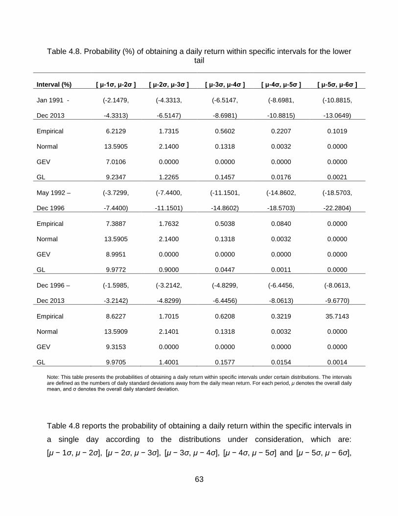
63

Table 4.8. Probability (%) of obtaining a daily return within specific intervals for the lower tail

Interval (%) [ μ-1σ, μ-2σ ] [ μ-2σ, μ-3σ ] [ μ-3σ, μ-4σ ] [ μ-4σ, μ-5σ ] [ μ-5σ, μ-6σ ]

Jan 1991 -

Dec 2013

(-2.1479,

-4.3313)

(-4.3313,

-6.5147)

(-6.5147,

-8.6981)

(-8.6981,

-10.8815)

(-10.8815,

-13.0649)

Empirical 6.2129 1.7315 0.5602 0.2207 0.1019

Normal 13.5905 2.1400 0.1318 0.0032 0.0000

GEV 7.0106 0.0000 0.0000 0.0000 0.0000

GL 9.2347 1.2265 0.1457 0.0176 0.0021

May 1992 –

Dec 1996

(-3.7299,

-7.4400)

(-7.4400,

-11.1501)

(-11.1501,

-14.8602)

(-14.8602,

-18.5703)

(-18.5703,

-22.2804)

Empirical 7.3887 1.7632 0.5038 0.0840 0.0000

Normal 13.5905 2.1400 0.1318 0.0032 0.0000

GEV 8.9951 0.0000 0.0000 0.0000 0.0000

GL 9.9772 0.9000 0.0447 0.0011 0.0000

Dec 1996 –

Dec 2013

(-1.5985,

-3.2142)

(-3.2142,

-4.8299)

(-4.8299,

-6.4456)

(-6.4456,

-8.0613)

(-8.0613,

-9.6770)

Empirical 8.6227 1.7015 0.6208 0.3219 35.7143

Normal 13.5909 2.1401 0.1318 0.0032 0.0000

GEV 9.3153 0.0000 0.0000 0.0000 0.0000

GL 9.9705 1.4001 0.1577 0.0154 0.0014

Note: This table presents the probabilities of obtaining a daily return within specific intervals under certain distributions. The intervals are defined as the numbers of daily standard deviations away from the daily mean return. For each period, μ denotes the overall daily mean, and σ denotes the overall daily standard deviation.

Table 4.8 reports the probability of obtaining a daily return within the specific intervals in

a single day according to the distributions under consideration, which are:

[μ − 1σ, μ − 2σ], [μ − 2σ, μ − 3σ], [μ − 3σ, μ − 4σ], [μ − 4σ, μ − 5σ] and [μ − 5σ, μ − 6σ],

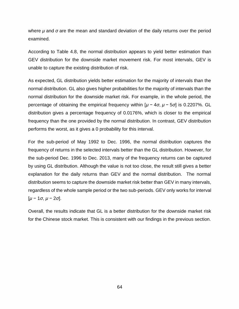
64

where μ and σ are the mean and standard deviation of the daily returns over the period

examined.

According to Table 4.8, the normal distribution appears to yield better estimation than

GEV distribution for the downside market movement risk. For most intervals, GEV is

unable to capture the existing distribution of risk.

As expected, GL distribution yields better estimation for the majority of intervals than the

normal distribution. GL also gives higher probabilities for the majority of intervals than the

normal distribution for the downside market risk. For example, in the whole period, the

percentage of obtaining the empirical frequency within [μ − 4σ, μ − 5σ] is 0.2207%. GL

distribution gives a percentage frequency of 0.0176%, which is closer to the empirical

frequency than the one provided by the normal distribution. In contrast, GEV distribution

performs the worst, as it gives a 0 probability for this interval.

For the sub-period of May 1992 to Dec. 1996, the normal distribution captures the

frequency of returns in the selected intervals better than the GL distribution. However, for

the sub-period Dec. 1996 to Dec. 2013, many of the frequency returns can be captured

by using GL distribution. Although the value is not too close, the result still gives a better

explanation for the daily returns than GEV and the normal distribution. The normal

distribution seems to capture the downside market risk better than GEV in many intervals,

regardless of the whole sample period or the two sub-periods. GEV only works for interval

[μ − 1σ, μ − 2σ].

Overall, the results indicate that GL is a better distribution for the downside market risk

for the Chinese stock market. This is consistent with our findings in the previous section.

65

Figure 4.6. A comparison of the normal, GEV and GL distributions

Figure 4.6 illustrates the difference that the extreme value analysis can make to the VaR

calculation. This figure indicates the lower tail of the daily returns of the Shanghai Stock

Composite Index from 1991 to 2013. We plot the cumulative density function (CDF) of the

GL, GEV and the normal for the comparison purpose. The monthly minima of the daily

returns are used to estimate the parameters of each distribution.

According to Figure 4.6, the GL distribution behaves similarly to the SSE Composite

Index, whereas the GEV and normal distributions are more apart from the actual

observations. As a result, the normality or GEV distribution assumption may lead to

severe underestimation of market risk.

4.7. Summary and Concluding Remarks

In this paper, we model the empirical distribution of the extreme daily stock returns in the

Chinese stock market over the period 1991 to 2013 by applying the EVT. The Chinese

stock market is considered due to its importance and its unique features as an emerging

market.

66

This study is carried out using the BMM method instead of the often used POT method.

Our research reveals that the GEV distribution is the best fit for modeling the extreme

upward stock market movements, while GL is the best fit for modeling the extreme

downward stock market movements. Further, the sub-period analysis indicates that this

conclusion holds regardless of the daily share price restriction and the GFC. It is also

demonstrated that our findings can improve the VaR calculation for the Chinese stock

market, which can have important implications for the stock market risk management.

Our findings for the Chinese stock market are different from the findings for other markets

in the literature. GEV and GL distributions are found to be good to model the extreme

upside and downside market movements for China, respectively. However, one

distribution is normally found to be the best to model both types of extreme movements

for other markets in the literature. This may be due to the unique features associated with

the Chinese stock market. For example, the effective free-float of the shares in the

Chinese market is low. Approximately 70 percent of the shares are non-tradable and held

by the government, state-owned enterprise (SOEs) and Chinese institutions. The

restricted number of shares available for domestic investors implies a possible artificially

strong demand in the Chinese stock market. This is further fuelled by the strong increase

in economic wealth (GDP) together with limited alternative investments opportunities and

the high savings rate of the Chinese population (Mitchell and Ong, 2006). These empirical

findings provide a new understanding of the best distribution to describe extreme behavior

for the Chinese stock market.

In addition, our research provides support to the claim that GL distribution does deserve

the serious consideration of financial risk analysts in modeling extreme stock market

movements (Tolikas and Gettingby, 2009).

It is also demonstrated that there is no long-term change with respect to the best

distributions of extreme stock returns in the Chinese stock market due to the stock

movement restriction or the GFC, although a significant impact is found during the GFC

period. These findings can bring new information for investors or risk managers to

understand the current situation in the Chinese stock market and help to improve the

measurement of stock market risk.

67

Finally, we would like to note that this study has a narrow focus and that it is only the first

step in modeling the extreme returns in the Chinese stock market. The research

presented in this paper can be extended in several aspects. For example, further research

can be carried out to compare the EVT approach with the GARCH-based approach in

estimating VaR. One can apply the conditional EVT and conditional correlation and

copulas (CCC) to investigate the dependency between the Chinese stock market and

other major global stock markets. These are left for a future research.

68

4.8. References

Allen, DE, Singh, AK & Powell, RJ 2013, 'EVT and tail-risk modelling: Evidence from

market indices and volatility series', The North American Journal of Economics and

Finance.

Arshad, M, Rasool, MT & Ahmad, MI 2003, 'Anderson Darling and Modified Anderson

Darling Tests for Generalized Pareto Distribution', Pakistan Journal of Applied

Sciences, vol. 3, no. 2, pp. 85-8.

Basel Committee on Banking Supervision 1996, 'Overview of the amendment to the

capital accord to incorporate market risk', Bank for International Settlements.

Black, F & Myron, S 1973, 'The Pricing of Options and Corporate Liabilities', Journal of

Political Economy, vol. 81, no. 3, pp. 637-54.

Chan, K, Menkveld, AJ & Yang, Z 2006, 'Are domestic investors more informed than

foreign investors', Journal of Financial Markets.

Chen, L, Li, S & Lin, W 2007, The impact of the opening up of the B-share markets on

the integration of Chinese stock markets, vol. 8, Emerald Group Publishing Limited.

Chong, TT-L, Lam, T-H & Yan, IK-M 2012, 'Is the Chinese stock market really inefficient?',

China Economic Review, vol. 23, no. 1, pp. 122-37.

Cotter, J 2007, 'Extreme risk in Asian equity markets'.

D'Agostino, RB & Stephens, MA 1986, Goodness-of-fit Technicques, vol. 68, CRC press.

Dungey, M & Zhumabekova, D 2001, 'Testing for contagion using correlations: some

words of caution (No. 2001-09)'. Federal Reserve Bank of San Francisco.

Embrechts, P, Resnick, SI & Samorodnitsky, G 1999, 'Extreme value theory as a risk

management tool', North American Actuarial Journal, vol. 3, no. 2, pp. 30-41.

69

Eun, CS & Huang, W 2007, 'Asset pricing in China's domestic stock markets: Is there a

logic?', Pacific-Basin Finance Journal, vol. 15, no. 5, pp. 452-80.

Fisher, RA & Tippett, LHC 1928, 'Limiting forms of the frequency distribution of the largest

or smallest member of a sample', paper presented to Mathematical Proceedings of

the Cambridge Philosophical Society.

Gençay, R & Selçuk, F 2004, 'Extreme value theory and Value-at-Risk: Relative

performance in emerging markets', International Journal of Forecasting, vol. 20, no.

2, pp. 287-303.

Gettinby, G, Sinclair, C, Power, D & Brown, R 2006, 'An analysis of the distribution of

extremes in indices of share returns in the US, UK and Japan from 1963 to 2000',

International Journal of Finance & Economics, vol. 11, no. 2, pp. 97-113.

Gettinby, G, Sinclair, C, Power, DM & Brown, R 2004, 'An analysis of the distribution of

extreme share returns in the UK from 1975 to 2000', Journal of Business Finance &

Accounting, vol. 31, no. 5‐6, pp. 607-46.

Hosking, J 1986, 'The theory of probability weighted moments', Research Rep. RC, vol.

12210, p. 160.

Hosking, J, Wallis, JR & Wood, EF 1985, 'Estimation of the generalized extreme-value

distribution by the method of probability-weighted moments', Technometrics, vol. 27,

no. 3, pp. 251-61.

Hosking, JR 1990, 'L-moments: analysis and estimation of distributions using linear

combinations of order statistics', Journal of the Royal Statistical Society. Series B

(Methodological), pp. 105-24.

Hosking, JR & Wallis, JR 1987, 'Parameter and quantile estimation for the generalized

Pareto distribution', Technometrics, vol. 29, no. 3, pp. 339-49.

70

Jansen, DW & De Vries, CG 1991, 'On the frequency of large stock returns: Putting

booms and busts into perspective', The review of economics and statistics, pp. 18-

24.

Jondeau, E & Rockinger, M 2003, 'Testing for differences in the tails of stock-market

returns', Journal of Empirical Finance, vol. 10, no. 5, pp. 559-81.

Kang, J, Liu, M-H & Ni, SX 2002, 'Contrarian and momentum strategies in the China stock

market: 1993–2000', Pacific-Basin Finance Journal, vol. 10, no. 3, pp. 243-65.

Karmakar, M 2013, 'Estimation of tail-related risk measures in Indian stock market: An

extreme value approach', Review of Financial Economics.

Longin, FM 1996, 'The Asymptotic Distribution of Extreme Stock Market Returns', The

Journal of Business, vol. 69, no. 3, pp. 383-408.

Los, CA & Yu, B 2008, 'Persistence characteristics of the Chinese stock markets',

International Review of Financial Analysis, vol. 17, no. 1, pp. 64-82.

Marimoutou, V, Raggad, B & Trabelsi, A 2009, 'Extreme Value Theory and Value at Risk:

Application to oil market', Energy Economics, vol. 31, no. 4, pp. 519-30.

Markowitz, H 1952, 'Portfolio Selection*', The Journal of Finance, vol. 7, no. 1, pp. 77-91.

Merton, RC 1973, 'An Intertemporal Capital Asset Pricing Model', Econometrica, vol. 41,

no. 5, pp. 867-87.

Mitchell, JD & Ong, LL 2006, Seasonalities in China's Stock Markets: Cultural Or

Structural?, International Monetary Fund.

Moharram, S, Gosain, A & Kapoor, P 1993, 'A comparative study for the estimators of the

generalized Pareto distribution', Journal of Hydrology, vol. 150, no. 1, pp. 169-85.

Mookerjee, R & Yu, Q 1999, 'An empirical analysis of the equity markets in China', Review

of Financial Economics, vol. 8, no. 1, pp. 41-60.

71

Naughton, T, Truong, C & Veeraraghavan, M 2008, 'Momentum strategies and stock

returns: Chinese evidence', Pacific-Basin Finance Journal, vol. 16, no. 4, pp. 476-

92.

Parkinson, M 1980, 'The extreme value method for estimating the variance of the rate of

return', Journal of Business, vol. 53, no. 1, pp. 61-5.

Peel, MC, Wang, Q, Vogel, RM & McMahon, TA 2001, 'The utility of L-moment ratio

diagrams for selecting a regional probability distribution', Hydrological sciences

journal, vol. 46, no. 1, pp. 147-55.

Poon, S-H, Rockinger, M & Tawn, J 2004, 'Extreme value dependence in financial

markets: Diagnostics, models, and financial implications', Review of Financial

Studies, vol. 17, no. 2, pp. 581-610.

Sharpe, WF 1964, 'Capital Asset Prices: A Theory Of Market Equilibrium Under

Conditions Of Risk*', The Journal of Finance, vol. 19, no. 3, pp. 425-42.

Tolikas, K 2008, 'Value-at-risk and extreme value distributions for financial returns',

Journal of Risk, vol. 10, no. 3, p. 31.

Tolikas, K & Gettinby, GD 2009, 'Modelling the distribution of the extreme share returns

in Singapore', Journal of Empirical Finance, vol. 16, no. 2, pp. 254-63.

Wen, X, Wei, Y & Huang, D 2012, 'Measuring contagion between energy market and

stock market during financial crisis: A copula approach', Energy Economics, 34(5),

1435-1446.

Xu, CK 2000, 'The microstructure of the Chinese stock market', China Economic Review,

vol. 11, no. 1, pp. 79-97.

Zhu, J 2006, 'Testing for Expected Return and Market Price of Risk in Chinese A&B Share

Markets: nA Geometric Brownian Motion and Multivariate GARCH Model Approach'.

73

CHAPTER 5: THE DEPENDENCE

STRUCTURE BETWEEN CHINESE AND

OTHER MAJOR STOCK MARKETS

USING EXTREME VALUES AND

COPULAS

This study employs the extreme value theory (EVT) and stochastic copulas to investigate

the dependence structure between the Chinese stock market and other major stock

markets including the US, Canada, UK, Germany, Japan and Australia. Our research

reveals that the dependence between the Chinese stock market and the developed

markets is low. Furthermore, our study indicates Chinese stock market has stronger

dependence with Asia and Europe than the US. Among all 6 pairs, the dependence

between Chinese and US stock markets is the lowest and that between China and

Australia is the highest. It is also found that US and UK do not have significant upper tail

dependence with Chinese stock market and the dependence between China and Japan

is strong but has weakened since 2012. Overall, diversification across all 6 pairs of stock

markets is not effective.

Keywords: Copula, Extreme value theory, Dependence structure, Chinese stock market

This chapter is reproduced from a paper under review by International Review of Economics & Finance. This chapter has its

reference section and style according to this particular journal’s requirements. To accommodate with the thesis flow, figure numbers

have been changed and differ from the original submission draft.

74

5.1. Introduction

In recent years, the dependence structure between stock markets has attracted more and

more attention due to the highly volatility and fat tailed distributions associated with the

markets. An increase in dependence or correlation can increase the prospect of financial

losses. In particular, the existence of asymmetric dependence structure in some periods

can have an important impact on international diversification. Therefore, it is important to

understand the dependence structure between stock markets for investment and risk

management.

Many studies have been done on the dependence structure and most of them tend to

focus on the developed markets (Longin and Solnik, 2001; Ang and Chen, 2002; Ane and

Labidi 2006; Jondeau and Rockinger 2006; Bartram et al. 2007; Bhatti & Nguyen 2012).

However, few studies have been done on the emerging markets including the Chinese

stock market.

In this paper, we focus on the Chinese stock market for the following reasons. First, China

is the world's second largest economy and it has a close relationship with the rest of the

world in terms of international trade and investment. Therefore, any change in the

Chinese stock market can have important impact to others. The Chinese stock market

has experienced drastic changes since 1990 (He, Wang, & Wu 2013) and is still an

emerging market. The Chinese stock market will be more and more influential in the

world as the Chinese economy grows.

Second, the Chinese stock market has some unique features which make this study

interesting and challenging. There are two main stock exchanges in China: the Shanghai

Stock Exchange (SHSE) and the Shenzhen Stock Exchange (SZSE). Most companies

listed on the SHSE are state-owned and large while those on the SZSE are mostly small

and export-oriented joint-ventures. There are two classes of shares listed and traded on

both exchanges and these are known as A- and B-shares. A-shares are restricted to local

or domestic investors while B shares are only available to foreign investors. US dollars

have been used as the foreign currency for B-shares on SHSE and Hong Kong dollars

75

for B-shares on SZSE. Opening up the B-share market to domestic investors in 2001 has

been considered a very important government initiative to integrate Chinese stock

markets with the rest of the world. In this study, we use the CSI300 Composite Index to

represent the overall performance of Chinese stock market. This index was introduced

on April 8, 2005 and consists of 300 stocks traded in the Shanghai and Shenzhen stock

exchanges.

Third, the Chinese stock market is often very volatile due to excessive speculation. The

major force driving Chinese stock market movements is the retail investors who bring the

noise to the market although the role of both domestic and foreign institutional investors

is growing in recent years. For example, the Shanghai Stock Exchange (SSE) composite

index was stagnant between 2010 and 2013, but increased sharply by almost 60% in

2014.

A few studies regarding the dependence between Chinese and other stock markets can

be found in the literature. Chan, Fung, and Thapa (2007) illustrated how the financial

market in China has emulated and become integrated with developed markets over time.

In contrast, Li (2007) demonstrated that the Chinese stock market was weakly integrated

with regional or developed markets. Using asymmetric data, Hyde et al. (2007) found a

significant correlation between stock markets in Asian-Pacific countries, Europe, and the

US according to the dynamic conditional correlation GARCH model (AG-DCC-

GARCH). Hu (2010) discovered that the dynamic dependence structure between the

Chinese and US financial markets is quite volatile. Lai and Tseng (2010) observed there

is no significant dependence between China and the G7 countries. In sum, most studies

tend to look at the dependence structure between the Chinese and US stock markets. In

contrast, this study aims to consider dependence structure between China and all other

major stock markets.

To date, many methods and models have been used to examine the dependence

structure between stock markets (Embrechts et al. 2001; Jondeau and Rockinger 2006;

Chen and Fan 2006; Longin and Solnik 2001; Patton 2006a &b; Rodriguez 2007).

However, these methods all have some drawbacks and limitations. In particular, some

76

methods neglect the stylised facts of returns and ignore the non-linearity in the financial

data. This research aims to model the dependence structure between stock markets

using both Extreme Value Theory (EVT) and time-varying copulas.

EVT is a well-known tool that can capture extreme circumstances. As shown in Hussain

and Li (2015), EVT can be useful in modelling the extreme returns of stock markets. On

the other hand, copula approach is a good choice for modelling the dependence between

stock markets as it allows the use of a variety of marginal distributions without the

normality limitation and builds more accurate information into joint distribution. Thus

combing copula approach with EVT can be an effective way to model the dependence

between stock markets.

So far, little is known about the dynamic dependence structure of the Chinese stock

market with those of developed countries. This paper aims to enrich the literature.

Specifically, this study explores the dependence structure between the CSI300 Index

(China) and a set of 6 major stock market indices: S&P500 (US), TSX Composite Index

(Canada), FTSE100 (UK), Nikkei 225 (Japan) and ASX200 (Australia) for the period July

1, 2005 to June 30, 2015.

We find that the dependence between the Chinese stock market and the developed

markets is still low. Furthermore, our study indicates Chinese stock market seems to have

stronger dependence with Asia and Europe than the US. Among all 6 pairs, the

dependence between Chinese and US stock markets is the lowest and that between

China and Australia is the highest. It is also found that US and UK do not have significant

upper tail dependence with Chinese stock market and the dependence between China

and Japan is strong but has weakened since 2012. Overall, diversification across all 6

pairs of stock markets is not effective.

The remainder of this paper is organised as follows. The next section explains the

theoretical background. The methodology is discussed in Section 5.3. Section 5.4

describes the data and sample descriptive statistics. Section 5.5 presents the empirical

results. Finally, Section 5.6 provides some concluding remarks.

77

5.2.Theoretical Background

This section discusses the details of the theoretical approach used in this research.

5.2.1. Extreme Value Theory

Extreme Value Theory (EVT) is a well-known tool that can capture extreme

circumstances. EVT method has been used widely in hydrology, weather, insurance

coverage, engineering and ecological analysis. The earliest studies done on EVT include

Embrechts et al. (1999) and Poon et al. (2004). Many studies applying EVT in finance

can also be found in the literature, e.g. Longin (1996), Danielsson and de Vries (2000),

Straetmans (1998), McNeil (1999), Neftci (2000), McNeil (1998), McNeil and Frey (2000),

Gencay et al. (2003) and Hussain and Li (2015).

EVT is a technique that focuses on the tail rather than the whole of distribution. In our

analysis, we employ the peaks over threshold (POT) method to improve the tail of the

distribution for each series. The POT approach works by sorting clustered phenomena

that are frequently found in the real world. Identifying a suitable threshold is the crucial

process in POT. A trade-off between bias and variance is required to find the optimal

threshold. In this research, the observed excesses over the threshold will be fitted to the

Generalized Pareto Distribution (GPD) according to the theorem below.

Let (𝑥1, 𝑥2, … ) be a sequence of independent and identically distributed random variables

with the distribution function 𝐹. Then for a large class of underlying distribution 𝐹 and

large 𝑢, the conditional excess distribution function 𝐹𝑢 can be approximated by GPD, that

is:

𝐹𝑢(𝑦) ≈ 𝐺𝜉,𝛼(𝑦), 𝑢 → ∞

where

78

𝐺𝜉,𝛼(𝑦) = {1 − (1 +

𝜉𝑦

𝛼)

−1𝜉 𝑖𝑓 𝜉 ≠ 0

1 − 𝑒−𝑦𝛼 𝑖𝑓 𝜉 = 0

( 5.1 )

For 𝑦 ≥ 0 when ξ ≥ 0 and 0 ≤ y ≤ (−𝛼

𝜉) when ξ < 0. α is the scale parameter, ξ is the shape

parameter for the GPD.

For details on the above theorem, we refer to Balkema and De Haan (1974) and Pickands

(1975).

5.2.2. Copula Models

Copula theory was first introduced by Sklar (1959). It was first applied in finance during

the early 2000s (Cherubini et al. 2004). Recently, copula models have been widely used

to understand the asymmetric dependence structures between stock markets. A key

feature of copula models is that there is no normality assumption. Given that the stock

returns are often not normal, Copula models can thus be suitable for modelling the

dependence between stock markets.

A copula allows us to decompose an n-dimensional joint distribution into its marginal

distributions. The flexibility behind the assumption and the ability to extract information

regarding dependence structure from the joint probability distribution function, have

enabled it to be widely used in various applications. Mathematically, a bivariate copula

that is used in this study can be written as:

F (x1, x2 ) = C ( F ( x1 ),F( x2 )) ( 5.2 )

where C is the copula employed to compose F with random variables of x1, x2 into marginal

distributions.

79

There are many copulas available. However, given our objectives, we consider only

Gaussian and Symmetrised Joe–Clayton (SJC) copulas in this paper. Gaussian copula

is used to capture the overall dependence between the markets and (SJC) copula is used

to capture the behaviour of the upper and lower tails.

5.3. Methodology

The methodology for this study can be divided into two main parts: marginal distribution

and dependence structure. First, we need to specify the functional form of the marginal

distributions. Then, the dependence between the variables will be determined with the

appropriate copula function.

5.3.1. Marginal Distribution Estimation

In this paper, we use GJR-GARCH model with the mean return modelled as an AR(1)

process (Engle and Ng 1993; Glosten et al. 1993). Let 𝑟𝑡 denote the returns and ℎ𝑡2 denote

the conditional variance for the period of 𝑡. The GJR-GARCH model8 can be formulated

as follows:

𝑟𝑡 = 𝜇 + 𝜗𝑟𝑡−1 + 휀𝑡

ℎ𝑡2 = 𝑐 + 𝛾ℎ𝑡−1

2 + 𝜂1휀𝑡−12 + 𝜂2𝑠𝑡−1휀𝑡−1

2

( 5.3 )

( 5.4 )

where 𝑠𝑡−1 = 1 when 휀𝑡−1 is negative and 0 otherwise. Let 𝑑𝑓 represent the degree of

freedom and Ωt-1 denote the previous information set. The standardize residual of series,

𝑧𝑡 are modelled as a Student t distribution:

8 Other GARCH models can also be used to compensate for the heteroskedasticity of the returns.

80

𝑧𝑡|Ω 𝑡−1 = √𝑑𝑓

𝜎𝑡2(𝑑𝑓 − 2)

휀𝑡𝑧𝑡~𝑖𝑖𝑑 𝑡𝑑𝑓

( 5.5 )

To model the tail behaviour of returns, the residuals that exceed a predefined threshold

at level 𝑢 , is modelled via GPD. This combination (empirical distribution of GJR-GARCH

for interior part of the marginal distribution and EVT for the tails) is known as conditional

EVT. Many methods have been proposed to determine the suitable threshold value 𝑢

(Neftci 2000; McNeil and Frey 2000; Longin and Solnik 2001). We use 10th and 90th

percentile of the whole sample as suggested by Du Monchel (1983).

In sum, the cumulative function of GARCH-EVT can be written as:

𝐹(𝑧) =

{

𝑘𝐿

𝑛(1 + 𝜉

𝑢𝐿 − 𝑧

α)−1

𝜉⁄ for 𝑧 < 𝑢𝐿 ,

∅(𝑧) for 𝑢𝐿 < 𝑧 < 𝑢𝑈

1 −𝑘𝑈

𝑛(1 + 𝜉

𝑧 − 𝑢𝑈

α)−1

𝜉⁄ for 𝑧 > 𝑢𝑈 ,

( 5.6 )

where α is the scale parameter, 𝜉 is the shape parameter, 𝑢𝐿 (𝑢𝑈) is the lower (upper)

threshold, n is the number of observations, ∅ is the empirical distribution function and

𝑘𝐿(𝑘𝑈) is the number of observations below(exceeding) the threshold 𝑢𝐿 (𝑢𝑈).

5.3.2. Copula Estimation

In this study, we use both constant and time-varying copulas (Gaussian and SJC) to

examine the dependence structure between the China-related pairs of stock market

return series.

81

5.3.2.1. Gaussian Copula

Gaussian copula is a well-known copula used in finance and it is associated with

multivariate normal distribution. In the bivariate case, the random vector of random

variables 𝑢 and 𝑣 can be considered bivariate normal if both 𝑢 and 𝑣 are normal.

Therefore the dependence structure based on Gaussian copula can be written as:

𝐶(𝑢, 𝑣) = ∫ ∫1

2𝜋√1 − 𝛿2

ᶲ−1(𝑣)

−∞


2(1 − 𝛿2)} 𝑑𝑥𝑑𝑦

ᶲ−1(𝑢)

−∞

𝐶 = Φ𝛿(Φ−1(𝑢),Φ−1(𝑣)),−1 ≤ 𝛿 ≤ 1

( 5.7 )

( 5.8 )

where Φ and Φ𝛿 are the standard normal CDF’s and 𝛿 is the linear correlation coefficient

between 𝑢 and 𝑣.

For the time-varying copula, the Gaussian dependence parameter is assumed to evolve

over time according to Patton’s (2006a):

𝛿𝑡 = 𝜆(𝜔 + 𝛽𝛿𝑡−1 + 𝛼1

10∑[Φ−1(𝑢𝑡−𝑗)Φ

−1(𝑣𝑡−𝑗)]

10

𝑗=1

)

( 5.9 )

where 𝜆 = (1 − 𝑒−𝑥)/(1 + 𝑒−𝑥) is the modified logistic transformation to ensure 𝛿𝑡 in the

interval (-1,1). Note that in Equation (8), an ARMA (1,10) type process is assumed and

𝛽𝛿𝑡−1 captures the persistence effect and the mean of the product of the last 10

observations of the transformed variables Φ−1(𝑢𝑡−𝑗) and Φ−1(𝑣𝑡−𝑗) captures the


82

5.3.2.2. Symmetrised Joe–Clayton Copula (SJC Copula)

The SJC copula is a modified version of the 1997 Joe–Clayton copula. In general, the

Joe-Clayton copula can be defined as:


−1

𝛾 )1/k ( 5.10 )

where

𝑘 =1


𝛾 = −1


( 5.11 )

( 5.12 )

and

𝜏𝑈𝜖( 0 ,1 ), 𝜏𝐿𝜖 (0 , 1 ). ( 5.13 )

The original Joe–Clayton copula is not as attractive as the SJC copula because the SJC

copula can be used to explore the lower and upper tail dependence simultaneously.

Consequently the SJC copula is the ideal choice for understanding the tail behaviour and

the SJC copula can be written in the following form:


𝑈, 𝜏𝐿) + 𝐶𝐽𝐶(1 − 𝑢, 1 − 𝑣|𝜏𝑈 , 𝜏𝐿) + 𝑢 + 𝑣 − 1] ( 5.14 )

where 𝐶𝐽𝐶 is the Joe–Clayton copula and 𝜏𝑈 and 𝜏𝐿 represent the upper and lower tail

dependence, respectively.

For the time-varying copula, the evolution parameters for the SJC copula can be defined

according to Patton (2006a):

83


1

10∑ |𝑢1,𝑡−𝑖 − 𝑢2,𝑡−𝑖|

10

𝑖=1)

( 5.15 )

where �̃� is given as the logistic transformation: �̃�(𝑥) = (1 + 𝑒−𝑥)−1, which ensures the

dependence parameter 𝜏𝑈/𝐿 in (0,1).

5.3.3. Estimation Method

5.3.3.1. Marginal Estimation

The Maximum Likelihood Estimation (MLE) is used to estimate the parameters for the

marginal distributions. Based on (6), the full estimation of the combination of the

parametric and GPD distributions can be written as:

�̂�(𝑧) =

{

𝑘𝐿

𝑛(1 + 𝜉

𝑢𝐿 − 𝑧

α̂)−1

ξ̂⁄ for 𝑧 < 𝑢𝐿 ,

∅(𝑧) for 𝑢𝐿 < 𝑧 < 𝑢𝑈,

1 −𝑘𝑈

𝑛(1 + ξ̂

𝑧 − 𝑢𝑈

α̂)−1

ξ̂⁄ for 𝑧 > 𝑢𝑈 ,

( 5.16 )

where α̂ and 𝜉 denote the MLE of α and 𝜉, respectively.

5.3.3.2. The Inference Functions of Margins (IFM) for Copula

IFM method is used to estimate copula parameters due to several reasons. This method

is more flexible compared to MLE method. It also brings the advantage of assessing the

fit of the margin distribution separately. By contrast, MLE method needs extensive

computation which requires the parameters of the marginal distributions and the copula

functions to be estimated simultaneously.

There are two main steps with IFM method:

Step 1 : The parameters of the marginal distribution are estimated by using MLE:

84

𝜃𝑖 = arg𝑚𝑎𝑥𝑙𝑐(𝜃𝑖) = arg𝑚𝑎𝑥∑𝑙𝑜𝑔𝑓𝑖(𝑥𝑖, 𝜃𝑖)

𝑇

𝑡=1

( 5.17 )

where 𝑙𝑐 is the log-likelihood function of the marginal distribution Fi

Step 2 : The copula parameters 𝛿 are estimated in the next step based on the 𝜃𝑖:

𝛿 = arg𝑚𝑎𝑥𝑙𝑐(𝛿) = arg𝑚𝑎𝑥∑log (𝑐(𝐹1(𝑥1, 𝜃1),… , 𝐹𝑛(𝑥𝑛, 𝜃𝑛); 𝛿))

𝑇

𝑡=1

( 5.18 )

where 𝑙𝑐 is the likelihood function of the copula. The estimators are consistent under

standard regularity conditions.

5.3.4. Model Selection

In this research, we use Akaike Information Criterion (AIC) and Bayesian Information

Criterion (BIC) to select the best model for the copula.

AIC can be defined as:

AIC = −2 log( likelihood )+2k ( 5.19 )

where k is the number of parameters used in the model. AIC works based on the trade-

off between complexities and information lost when a given model is utilised to represent

the process that generates the data. The lower value of AIC, the closer is the fit of a model

to the empirical data.

BIC can be defined as:

85

BIC = −2 log( likelihood )+k·log(n) ( 5.20 )

where n is the number of data and k is the number of parameters used in the model. BIC

penalises model complexity more heavily compared to the AIC. The lowest value of BIC

indicates the best fit model.

5.4. Data and Descriptive Statistics

China Securities Index 300 stock index (CSI300) was officially launched on April 8, 2005.

This index consists of 300 stocks that represent approximately 70% of the total market

capitalisation of both the Shanghai and Shenzhen stock markets. Most shares in this

index are A-shares. This index reflects the performance of the Chinese A-share markets.

This study thus uses the CSI300 Composite Index as a representation of the Chinese

stock market.

The selection of other major stock markets is based on the consideration of demographic

location and market capitalization. The US and Canada stock markets are selected to

represent North America; the UK and Germany are selected to represent Europe; and

Japan and Australia are selected to represent Australasia. These stock markets are

among the major stock markets in the world. Consequently, the following stock indexes

are used for this study: S&P500 (US), TSX Composite Index (Canada), FTSE100 (UK),

DAX30 (Germany), Nikkei225 (Japan) and ASX200 (Australia). The daily closing index

levels from 1 July 2005 to 31 June 2015 are obtained from Datastream. The returns of

series can be calculated as 𝑟𝑡 = 𝑙𝑛𝑃𝑡 − 𝑙𝑛𝑃𝑡−1 where 𝑃𝑡 is the closing level of the index at

time t in our study. To compare the performance of all indices, we need to use the relative

daily index which is defined as the index normalised by using the initial index level for

each market index. Figure 5.1 illustrates the relative daily index series of the selected

stock markets for the whole sample period.

86

Figure 5.1. Relative daily index levels over the sample period

The data consists of 2607 daily observations over 10 years for each stock market. It is

worth noting that the sample period covers a few extreme volatile events in the financial

market including the Global Financial Crisis (GFC) and European Debt Crisis. As can be

seen from Figure 5.1, the volatility of the Chinese stock market is very high compared to

the others. Chinese stock market experienced an upward trend from 2006 to 2008 as the

other stock markets did. All the markets dropped dramatically between 2008 and 2009

due to the GFC.

A drastic upward trend began in early 2014 for the Chinese stock market. Two triggers

are behind this sharp rise9. First, the People’s Bank of China unexpectedly cut interest

9 See http://www.bbc.com/news/business-30708387, accessed on 9 December 2015.

http://www.bbc.com/news/business-30708387

87

rates for the first time in two years. The government’s monetary policy made the Chinese

stock market very attractive for investors who wanted to take advantage of this

opportunity. At the same time, the retail investors who make up about 80% of stock trading

volume in China have been moving money out of the main asset classes and property

into stocks. The second catalyst was the launch of Shanghai-Hong Kong Stock Connect.

This platform has enabled foreign investors to access and invest in the mainland market.

This trading scheme permits mainland investors to trade in Hong Kong stocks while

foreign investors can trade in the Shanghai market for the first time via the Hong

Kong stock exchange.

Table 5.1. Descriptive statistics of daily returns

China US Canada UK Germany Japan Australia

Mean 0.0633 0.0210 0.0148 0.0090 0.0331 0.0212 0.0094

Med 0.0250 0.0448 0.0544 0.0062 0.0745 0.0000 0.0093

Std 1.7790 1.2684 1.1712 1.2059 1.3943 1.5365 1.1247

Kurt 3.4250 11.4350 11.0487 8.5976 6.6651 8.8139 4.9777

Skew -0.4690 -0.3365 -0.7137 -0.1427 0.0341 -0.5782 -0.4251

Range 18.6260 20.4267 19.1582 18.6499 18.2309 25.3456 14.3325

Min -9.6952 -9.4695 -9.7880 -9.2656 -7.4335 -12.1110 -8.7043

Max 8.9309 10.9572 9.3703 9.3843 10.7975 13.2346 5.6282

JB Stat 1.363E+03 1.42E+04 1.34E+04 8.00E+03 4.80E+03 8.55E+03 2.76E+03

Count 2607 2607 2607 2607 2607 2607 2607

Mean, Med, Min, Max, Std, Skew and Kurt stand for the mean, median, minimum, maximum, the standard deviation, skewness and

kurtosis for each series, respectively. JB Stat denotes the statistics for the Jarque-Bera normality test with two degrees of freedom.

Table 5.1 presents the descriptive statistics of daily returns for the Chinese stock market

and those of the developed markets. The data are taken for the period from July 1, 2005

to June 31, 2015. The mean values for all stock markets are positive. Chinese stock

market has the highest value of mean with 0.0633% followed by Germany with 0.0331%.

The lowest mean belongs to the UK with 0.0090%. The standard deviation figures show

88

that Chinese stock market is very volatile compared to the others. The standard deviation

for Chinese stock market is 1.7790, followed by that of Japan, which is 1.5365. The lowest

value for the standard deviation belongs to Australia with 1.1247%. The US has the

highest value of kurtosis with 11.4350. This indicates the US market has highest

frequencies of the extreme returns. Referring to skewness, Australia has the highest with

0.0341 and Japan has the lowest with -0.5782. Positive skewness means the data has a

long tail to the right while negative skewness means the data has a long tail to the left.

The Jarque-Bera test results confirm that the return series are not normal for all markets.

In particular, the highest Jarque-Bera test statistic is reported for Japan.

In sum, Table 5.1 indicates that all return series exhibit some non-linear phenomenon

and extreme behaviour. The model that works on the normality assumption is thus not

appropriate.

Table 5.2. Linear correlation table


China 1

US 0.0693 1

Canada 0.1142 0.7412 1

UK 0.1499 0.5857 0.5784 1

Germany 0.1356 0.6256 0.5468 0.8586 1

Japan 0.2538 0.1143 0.2265 0.3254 0.2930 1

Australia 0.2684 0.1455 0.2347 0.3690 0.3173 0.6241 1

Table 5.2 reports the correlation coefficients between the return series. The linear

correlation values for the Chinese stock market related pair range between 0.0693 and

0.2684. Among the Chinese stock market related pairs, it is evident that the strongest

correlation is between China and Australia, followed by that between China and Japan.

Table 5.2 also shows that China appears to have a stronger correlation with Asia and

Europe than North America.

89

The weakest correlation is the one between China and US. Lower correlation is normally

associated effective diversification across the pair. This means that for investors in

Chinese Stock market, the US stock market may be a good choice for portfolio

diversification. However, this can be misleading and we need a better understanding of

the dependence between these markets which can be achieved by using copula

modelling. Upper and lower tail information used in copula modelling will enable us to

better comprehend the dependence structure between Chinese stock market and other

major stock markets.


The empirical results are presented in this section.

5.5.1. Estimating Marginal Models

In this study, the marginal distributions are estimated by using a semi-parametric

approach. This method is an innovation derived from GARCH methodology. First, the

estimated residuals are obtained as described in Section 5.3.1 and then we employ EVT

approach for the tail modelling. The values of the parameters obtained using GPD for the

upper and lower tails are presented in Table 5.3 below.

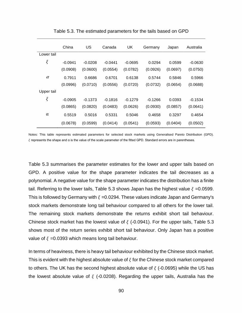
90

Table 5.3. The estimated parameters for the tails based on GPD


Lower tail

𝜉 -0.0941 -0.0208 -0.0441 -0.0695 0.0294 0.0599 -0.0630

(0.0908) (0.0600) (0.0554) (0.0782) (0.0926) (0.0697) (0.0750)

α 0.7911 0.6686 0.6701 0.6138 0.5744 0.5846 0.5966

(0.0996) (0.0710) (0.0556) (0.0720) (0.0732) (0.0654) (0.0688)

Upper tail

𝜉 -0.0905 -0.1373 -0.1816 -0.1279 -0.1266 0.0393 -0.1534

(0.0865) (0.0820) (0.0483) (0.0626) (0.0930) (0.0857) (0.0641)

α 0.5519 0.5016 0.5331 0.5046 0.4658 0.3297 0.4654

(0.0678) (0.0599) (0.0414) (0.0541) (0.0593) (0.0404) (0.0502)

Notes: This table represents estimated parameters for selected stock markets using Generalised Pareto Distribution (GPD). 𝜉 represents the shape and α is the value of the scale parameter of the fitted GPD. Standard errors are in parentheses.

Table 5.3 summarises the parameter estimates for the lower and upper tails based on

GPD. A positive value for the shape parameter indicates the tail decreases as a

polynomial. A negative value for the shape parameter indicates the distribution has a finite

tail. Referring to the lower tails, Table 5.3 shows Japan has the highest value 𝜉 =0.0599.

This is followed by Germany with 𝜉 =0.0294. These values indicate Japan and Germany's

stock markets demonstrate long tail behaviour compared to all others for the lower tail.

The remaining stock markets demonstrate the returns exhibit short tail behaviour.

Chinese stock market has the lowest value of 𝜉 (-0.0941). For the upper tails, Table 5.3

shows most of the return series exhibit short tail behaviour. Only Japan has a positive

value of 𝜉 =0.0393 which means long tail behaviour.

In terms of heaviness, there is heavy tail behaviour exhibited by the Chinese stock market.

This is evident with the highest absolute value of 𝜉 for the Chinese stock market compared

to others. The UK has the second highest absolute value of 𝜉 (-0.0695) while the US has

the lowest absolute value of 𝜉 (-0.0208). Regarding the upper tails, Australia has the

91

highest absolute value of 𝜉 (-0.1534). Japan has the lowest absolute value of 𝜉 (0.0393).

Based on these values, we can conclude that Chinese stock market is most likely to have

negative extreme returns while Australia is most likely to have positive extreme returns

among all seven stock markets considered. In other words, Chinese stock market has the

highest frequency for extreme negative returns while Australia stock market has the

highest frequency for extreme positive returns.

In general, the findings indicate that Chinese stock market has both heavy upper and

lower tails. This means that the Chinese stock market is volatile with both upside and

downside extreme returns. In contrast to the US and the UK, the upper tail is significantly

heavier than the lower tail for Chinese stock market.

Figure 5.2 plots the empirical Cumulative Distribution Function (CDF) of the exceedance

of the residuals for the upper tail along with the CDF from GPD for each selected stock

market. The fitted distributions closely follow the exceedance of the residuals although

only 10% of the standardised residuals are employed. Thus GPD appears to be a good

choice to model the upper tails. This is also valid for the lower tails10.

The overall CDF semi-parametric marginal distributions used in this study are shown in

Figure 5.3. As mentioned above, the tails are fitted by using EVT while the interior part is

estimated via a GARCH model. GARCH model is well suited for the interior body of the

distribution. However, this method seems to perform poorly in terms of tail modelling.

Combining it with EVT for the tails can overcome this problem.

In summary, Table 5.3 and Figures 5.2 and 5.3 demonstrate that our approach can

adequately model the marginal distributions of the return series for the stock markets

under consideration.

10 The results for the lower tails are similar and available upon request.

93

Figure 5.2. Upper tail distributions

94

Figure 5.3. Fitted overall distributions

5.5.2. Estimating the Copula Models

In this research, we are interested in the dependence structure between the Chinese

stock mark and other major stock markets with a focus on the behaviour of extreme

returns. To this end, both Gaussian copula and SJC copula as well as their dynamic

versions are employed.

95

Gaussian copula assesses the overall dependence structure while SJC copula helps us

to explore the behaviour of the lower and upper tails. In this research, Equation (9) is

used for the path of parameters (for Gaussian and SJC) (Patton, 2006a).

Table 5.4 provides an overview of parameter estimates for the Gaussian and SJC

copulas. 𝛿 (Gaussian), 𝜏𝑈 and 𝜏𝐿 (SJC) are the keys parameters for the constant copula.

For the time-varying copulas, the keys parameters are ω (Gaussian), 𝜔𝑈 and 𝜔𝐿 (SJC),

α (Gaussian), 𝛼𝑈 and 𝛼𝐿 (SJC) and β (Gaussian), 𝛽𝑈 and 𝛽𝐿 (SJC). ω (Gaussian), 𝜔𝑈

and 𝜔𝐿 (SJC) are used to describe the dependence level of each pair. The adjustment in

the dependence is captured by α (Gaussian), 𝛼𝑈 and 𝛼𝐿 (SJC). Lastly, parameter β

(Gaussian), 𝛽𝑈 and 𝛽𝐿 (SJC) are used to represent the degree of persistence of

dependence. The values for the AIC and BIC serve to identify the best model. A lower

value of AIC or BIC indicates a better fit. To assess the parameters path for every pair,

Figure 5.4 is used as well.

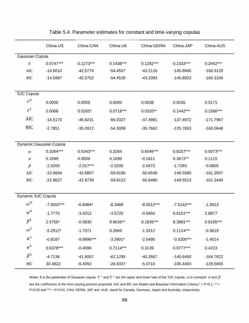
96

Table 5.4. Parameter estimates for constant and time-varying copulas

China-US China-CAN China-UK China-GERM China-JAP China-AUS

Gaussian Copula

𝛿 0.0747*** 0.1273*** 0.1438*** 0.1282*** 0.2333*** 0.2442***

AIC -14.6010 -42.5774 -54.4557 -43.2116 -145.8945 -160.3129

BIC -14.5987 -42.5752 -54.4535 -43.2093 -145.8923 -160.3106

SJC Copula

𝜏𝑈 0.0000 0.0059 0.0000 0.0038 0.0035 0.0171

𝜏𝐿 0.0068 0.0265* 0.0718*** 0.0320** 0.1442*** 0.1566***

AIC -14.5170 -46.8231 -66.0327 -47.4981 -137.4972 -171.7967

BIC -2.7851 -35.0912 -54.3008 -35.7662 -125.7653 -160.0648

Dynamic Gaussian Copula

ω 0.3264*** 0.5343*** 0.3264 0.6046*** 0.8257*** 0.5073***

α 0.1699 0.0659 0.1699 -0.1811 0.3672** 0.1115

β -2.0200 -2.017*** -2.0200 -2.0472 -1.7263 -0.0805

AIC -22.8694 -42.8807 -59.8190 -50.6548 -149.5580 -161.3507

BIC -22.8627 -42.8739 -59.8122 -50.6480 -149.5513 -161.3440

Dynamic SJC Copula

𝜔𝑈 -7.9552*** -6.8484* -8.3489 -8.0512*** -7.5142*** -1.5913

𝛼𝑈 -1.7770 -3.4312 -3.5720 -0.9450 0.6151*** 2.8877

𝛽𝐿 2.5755* -0.5830 9.8635** 9.1835*** 8.3881*** 0.8185***

𝜔𝐿 -5.2912* -1.7071 0.2669 -1.3312 0.1124*** -0.3619

𝛼𝐿 -0.8187 -9.9996*** -3.2891* -2.5490 -0.5200*** -1.4514

𝛼𝐿 0.6378*** -0.4096 0.7114*** 0.3139 0.9777*** 0.4223

𝛽𝐿 -4.7136 -41.6007 -62.1295 -40.2667 -140.6450 -164.7622

BIC 30.4822 -6.4050 -26.9337 -5.0710 -105.4493 -129.5665

Notes: δ is the parameter of Gaussian copula. 𝜏 U and 𝜏 U are the upper and lower tails of the SJC copula; ω is constant: α and β

are the coefficients of the time-varying process proposed. AIC and BIC are Akaike and Bayesian Information Criteria.* = P<0.1, ** =

P<0.05 and *** = P<0.01. CAN, GERM, JAP and AUS stand for Canada, Germany, Japan and Australia, respectively.

97

Figure 5.4 represents the evolution of the dependence parameters for each pair of

selected stock markets.

China-US

98

China-Canada

China-UK

99

China-Japan

China-Germany

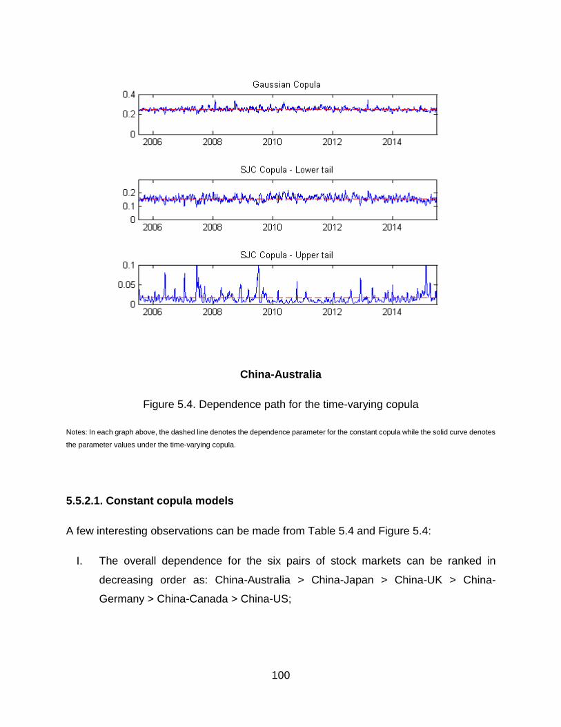
100

China-Australia

Figure 5.4. Dependence path for the time-varying copula

Notes: In each graph above, the dashed line denotes the dependence parameter for the constant copula while the solid curve denotes

the parameter values under the time-varying copula.

5.5.2.1. Constant copula models

A few interesting observations can be made from Table 5.4 and Figure 5.4:

I. The overall dependence for the six pairs of stock markets can be ranked in

decreasing order as: China-Australia > China-Japan > China-UK > China-

Germany > China-Canada > China-US;

101

II. The upper tail dependence for the six pairs can be ranked in decreasing order as:

China-Australia > China-Canada > China-Germany > China-Japan > China-US

and China-UK;

III. The lower tail dependence for the six pairs can be ranked in decreasing order as

follows: China-Australia > China-Japan > China-UK > China-Germany > China-

Canada > China-US.

The above rankings imply: i) China-Australia pair has the strongest overall and tail

dependence; ii) China-Japan pair has the second highest overall and lower tail

dependence and iii) The weakest dependence (overall or tail) is found between China

and the US.

Furthermore, this study reveals more insight regarding the dependence among the 6 pairs

of stock markets. China-Australia pair has the greater dependence compared to China-

Japan pair. From Table 5.4, the dependence of the Chinese stock market with the UK or

Germany is much stronger than that between China and US. This indicates Chinese stock

market is more dependent on the European stock markets compared to the US. Canada

stock market seems to have more dependence with the Chinese stock market compared

to the US stock market.

China-Australia pair has the greatest upper tail dependence. In contrast, the dependence

for the upper tails is low for China-US and China- UK. This indicates that the US and the

UK are not significantly affected by China or vice versa in the case of extreme positive

market movements. At the same time, it is apparent that 𝜏𝐿 is larger than 𝜏𝑈 for each

pair. This result demonstrates all 6 pairs have stronger lower tail dependence than upper

tail dependence.

A possible explanation for these results may come from the economic factors. China is

the largest exporter of goods in the world. It has created a huge demand for commodity

products and consequently has generated huge export booms in many markets.

Australian stock market is affected by China since its economy traditionally is driven by

resources and China has been the largest importer from Australia. In fact, 36% of

102

Australia’s exports went to China11. As a result, Chian-Australia pair has the strongest

dependence.

The lowest dependence structure between China and the US can be explained by their

trading relationship. It is evident that the US seems to have a cushion saving it from the

impact of Chinese economic volatility. The US is not greatly affected by declines in the

Chinese stock market. The US economic structure has a bilateral trade deficit with China

and the relationship is mostly one-way. The US imports three times as much from China

as it exports to China.

5.5.2.2. Time-varying copula models

In this section, the dynamic dependence structure of the six pairs of stock markets is

discussed. Figure 5.4 demonstrates the time paths for the overall, lower and upper tail

dependence by using both Gaussian and SJC copulas. In this study, the time variations

of dependence measures between return series are captured by the coefficients, α (𝛼𝐿

𝑜𝑟 𝛼𝑈) and β (𝛽𝐿 𝑜𝑟 𝛽𝑈) as in Equation (15). Based on the results for the time-varying

Gaussian copula model in Table 5.4, it can be seen that most of the time paths are close

to white noise as the values for the variation coefficient α are relatively higher than the

persistence coefficient β. However, for the SJC copula, all the persistence coefficient β is

larger than the variation coefficient α for all pairs. This outcome provides insights

regarding the changes of dependence structure for the upper and lower tails over the time

period.

For China-US pair, we can see the dependence parameter 𝛿𝑡 for the time-varying

Gaussian copula ranges between 0.05 and 0.15. These values are quite low compared

to the other pairs. The values of parameters for the time-varying SJC copula, 𝜏𝑈 and 𝜏𝐿

are almost zero. This indicates a low dependence for the upper and lower tail dependence

between these two markets. In sum, these results indicate that Chinese stock market has

low dependence with the US stock market (overall or tails).

11 See http://time.com/4014687/these-5-facts-explain-the-global-impact-of-chinas-impending-slowdown/, accessed on 9 December

2015

http://time.com/4014687/these-5-facts-explain-the-global-impact-of-chinas-impending-slowdown/

103

For the China-Canada pair, the values of dependence parameter 𝛿𝑡 in the time-varying

Gaussian copula model are between 0.1 and 0.2. This path of 𝛿𝑡is more stable

compared to the one for the China-US pair. In contrast, the lower dependence 𝜏𝐿 for this

pair seems to be more volatile. There are a few spikes as shown in Figure 5.4 which

range between 0.02 and 0.05. The values for 𝜏𝑈 are close to zero. Overall, Chinese stock

market seems to have a stronger dependence with the Canada stock market in terms of

lower tail dependence compared to the US.

For the China-UK pair, the values of dependence parameter 𝛿𝑡 in the time-varying

Gaussian copula are very volatile with 𝛿𝑡 moving between 0.1 and 0.2. These values are

slightly higher than those for the China-US pair. The path for 𝜏 𝐿 in the time-varying SJC

copula model ranges between 0.03 and 0.07. In contrast, the value for the upper tail is

almost zero.

For the China-Germany pair, Figure 5.4 reveals that the values of dependence parameter

𝛿𝑡 before 2007 are quite volatile and range between 0.05 and 0.2. The lower tail

dependence parameter for this pair ranges between 0.03 and 0.05. Similar to China-

Japan pair, the parameter 𝜏𝑈 for this pair is almost zero which indicates there is hardly

any dependence between these two markets in the case of positive extreme events. In

sum, these results provide important insight into the dependence of Chinese stock market

with the European stock markets.

Figure 5.4 also demonstrates the values for the parameter 𝛿𝑡 range between 0.3 and 0.4

for the China-Japan pair. These values are quite high compared to the ones for other

pairs. There is a significant dependence between Chinese stock market and Japanese

stock market in terms of lower dependence. We can see the values of 𝜏𝐿 range between

0.1 and 0.4. In contrast to the values of 𝜏𝐿, the values for the 𝜏𝑈 are almost zero. The

most striking result to emerge from these findings is regarding the behaviour of 𝜏𝐿. The

lower dependence for the China-Japan pair has become weaker starting in 2014.

Investors might become more aware with the drastic upward trend in Chinese stock

market in early 2014. To the best of our knowledge, this outcome has not been previously

documented.

104

Finally, China-Australia pair has the strongest dependence among all 6 pairs. The

parameter values for 𝛿𝑡 in the time-varying Gaussian copula are stable and fluctuating

around 0.25. The lower tail dependence parameter, 𝜏𝐿 for this pair also exhibits the same

characteristic and ranges between 0.1 and 0.2. The upper tail dependence parameter 𝜏𝐿

has a few peaks. These results are likely due to the strong Australia-China economic and

trade relationship during the sample period. China was Australia's largest two-way trading

partner in goods and services in 2014. The amount of Chinese investment in Australia in

2015 was more than fourteen times the level it was in 2005. The Australian federal

government has also been promoting its open investment regime and Foreign Investment

Review Board process12.

In this research, we are also interested in comprehending the opportunity to diversify

among the selected stock markets. To this end, the values of ω in the SJC copula model

need to be examined in detail. These values are useful for providing better insights into

active risk management practices for portfolio diversification (Wang et al. 2011). Based

on Table 5.4, all values of 𝜔𝐿 are relatively higher than 𝜔𝑈 for all 6 pairs of stock markets.

This can also be confirmed by observing the paths for the lower and the upper tail

dependence in Figure 5.4. Thus the dependence is stronger during a crisis for all 6 pairs

than during booming period. Risk diversification is thus not effective during a crisis. This

does have further implications for the financial risk management tools like VaR, expected

shortfall or other downside risk measures.

5.6. Concluding Remarks

Over the past few years, dependence structure between financial markets has been

actively studied. However, some methods employed are subject the normality

assumption. Most financial data tend to be non-linear, non-stationary and heavy-tailed.

Hence, suitable models that can incorporate these features are needed.

12 See http://china.embassy.gov.au/bjng/130716ecoandtrade.html, accessed on 9 December 2015.

http://china.embassy.gov.au/bjng/130716ecoandtrade.html

105

This study attempts to assess the dependence structure between the Chinese and other

major developed stock markets by using EVT and copula model. These methods can

provide more information compared to the linear correlation regarding understanding the

potential of risk diversification and risk management strategy.

Our results show that the Chinese stock market has higher levels of dependence with the

Asian and European markets than the US market. This outcome implies that the

probability of a downward extreme movement is high in these stock markets if there is a

downward extreme movement in the Chinese stock market and vice versa. This finding

might be attributed to the trading relationships and their geographical proximity.

This study also reveals that China-Australia pair has the strongest dependence and

China-Japan pair has the second highest dependence. However, the dependence

between China and Japan became weaker since the beginning of 2012.

This study enhances our understanding of Chinese stock market and its link to the

developed stock markets by exploring the tail behaviour. The research also makes a

contribution in terms of the diversification benefits. It is found that the dependence for

these pairs is much stronger during a crisis than during a booming period. Portfolio

diversification across these pairs during a downturn will not lead to many benefits. The

outcomes of this study thus have implications for policy-makers and risk management

practitioners. For example, this information can help investors to build confidence and

seek risk diversification opportunities in other asset classes.

Overall, this study makes a significant contribution to the literature. Further research can

be done by investigating the factors behind these relationships and the methodology

employed in this paper can be applied to computing Value at Risk (VaR) and optimal

portfolio weights.

106

5.7. References

Ané, T & Labidi, C 2006, 'Spillover effects and conditional dependence', International

Review of Economics and Finance, vol. 15, no. 4, pp. 417-42.

Balkema, AA & De Haan, L 1974, 'Residual life time at great age', Annals of Probability,

vol. 2, no. 5, pp. 792-804.

Bartram, SM, Taylor, SJ & Wang, YH 2007, 'The Euro and European financial market

dependence', Journal of Banking and Finance, vol. 31, no. 5, pp. 1461-81.

Bhatti, MI & Nguyen, CC 2012, 'Diversification evidence from international equity markets

using extreme values and stochastic copulas', Journal of International Financial

Markets, Institutions and Money, vol. 22, no. 3, pp. 622-46.

Chen, X & Fan, Y 2006, 'Estimation of copula-based semiparametric time series models',

Journal of Econometrics, vol. 130, no. 2, pp. 307-35.

Cheng, H & Glascock, JL 2005, 'Time-varying linkages between the greater China

economic area stock markets—Mainland China, Hong Kong, and Taiwan', Review of

Quantitative Finance and Accounting, vol. 24, no. 4, pp. 343-57.

Cherubini, U, Luciano, E & Vecchiato, W 2004, Copula methods in finance, John Wiley &

Sons.

Cheung, Y-W, Chinn, MD & Fujii, E 2003, 'China, Hong Kong, and Taiwan: A quantitative

assessment of real and financial integration', China Economic Review, vol. 14, no. 3,

pp. 281-303.

Cheung, YW, Chinn, MD & Fujii, E 2005, 'Dimensions of financial integration in greater

China: money markets, banks and policy effects', International Journal of Finance &

Economics, vol. 10, no. 2, pp. 117-32.

Danielsson, J & de Vries, CG 2000, 'Value-at-risk and extreme returns', Annales

D'Economie Et De Statistique, vol. 60, pp. 239-70.

107

Du Mouchel, W. H. (1983). Estimating the stable index α in order to measure tail

thickness: a critique. the Annals of Statistics, 1019-1031.

Embrechts, P, Lindskog, F & McNeil, A 2001, 'Modelling dependence with copulas and

applications to risk management', Modelling Dependence with Copulas and

Applications to Risk Management.



Engle, RF & Ng, VK 1993, 'Measuring and testing the impact of news on volatility', The

Journal of Finance, vol. 48, no. 5, pp. 1749-78.

Fermanian, JD 2005, 'Goodness-of-fit tests for copulas', Journal of Multivariate Analysis,

vol. 95, no. 1, pp. 119-52.


or smallest member of a sample', paper presented to Mathematical Proceedings of

the Cambridge Philosophical Society.

Gençay, R, Selçuk, F & Ulugülyaǧci, A 2003, 'High volatility, thick tails and extreme value

theory in value-at-risk estimation', Insurance: Mathematics and Economics, vol. 33,

no. 2, pp. 337-56.

Glosten, LR, Jagannathan, R & Runkle, DE 1993, 'On the relation between the expected

value and the volatility of the nominal excess return on stocks', The Journal of

Finance, vol. 48, no. 5, pp. 1779-801.

Hans, M 2007, 'Estimation and model selection of copulas with an application to exchange

rate', Estimation and model selection of copulas with an application to exchange rate.

Hu, J 2010, 'Dependence structures in Chinese and US financial markets: A time-varying

conditional copula approach', Applied Financial Economics, vol. 20, no. 7, pp. 561-

83.

108

Hussain, SI & Li, S 2015, 'Modeling the distribution of extreme returns in the Chinese

stock market', Journal of International Financial Markets, Institutions and Money, vol.

34, no. 0, pp. 263-76.

Hyde, S, Bredin, D & Nguyen, N 2007, Chapter 3 Correlation time-varyings between Asia-

Pacific, EU and US stock returns.

Johansson, AC & Ljungwall, C 2009, 'Spillover effects among the greater China stock

markets', World Development, vol. 37, no. 4, pp. 839-51.

Jondeau, E & Rockinger, M 2006, 'The Copula-GARCH model of conditional

dependencies: An international stock market application', Journal of international

money and finance, vol. 25, no. 5, pp. 827-53.

Li, H 2007, 'International linkages of the Chinese stock exchanges: A multivariate GARCH

analysis', Applied Financial Economics, vol. 17, no. 4, pp. 285-97.

Longin, F & Solnik, B 2001, 'Extreme correlation of international equity markets', Journal

of Finance, vol. 56, no. 2, pp. 649-76.

Longin, FM 1996, 'The asymptotic distribution of extreme stock market returns', Journal

of Business, vol. 69, no. 3, pp. 383-408.

McNeil, AJ 1998, 'Calculating quantile risk measures for financial time series using

extreme value theory', Calculating Quantile Risk Measures for Financial Return

Series Using Extreme Value Theory.

---- 1999, 'Extreme value theory for risk managers', Extreme Value Theory for Risk

Managers.

McNeil, AJ & Frey, R 2000, 'Estimation of tail-related risk measures for heteroscedastic

financial time series: An extreme value approach', Journal of Empirical Finance, vol.

7, no. 3-4, pp. 271-300.

109

Meissner, G 2013, Correlation Risk Modeling and Management: An Applied Guide

including the Basel III Correlation Framework - With Interactive Models in Excel /

VBA, Wiley.

Neftci, SN 2000, 'Value at risk calculations, extreme events, and tail estimation', Journal

of Derivatives, vol. 7, no. 3, pp. 23-37.

Nguyen, CC & Bhatti, MI 2012, 'Copula model dependency between oil prices and stock

markets: Evidence from China and Vietnam', Journal of International Financial


Patton, AJ 2006a, 'Modelling asymmetric exchange rate dependence', International

Economic Review, vol. 47, no. 2, pp. 527-56.

Patton, AJ 2006b, 'Estimation of multivariate models for time series of possibly different

lengths', Journal of Applied Econometrics, vol. 21, no. 2, pp. 147-73.

Pickands, J 1975, 'Statistical inference using extreme order statistics', Annals of

Statistics, vol. 3, no. 1, pp. 119-31.

Poon, SH, Rockinger, M & Tawn, J 2004, 'Extreme value dependence in financial


Studies, vol. 17, no. 2, pp. 581-610.

Rodriguez, JC 2007, 'Measuring financial contagion: A Copula approach', Journal of

Empirical Finance, vol. 14, no. 3, pp. 401-23.

Shin, K & Sohn, CH 2006, 'Trade and Financial Integration in East Asia: Effects on Co‐

movements', The World Economy, vol. 29, no. 12, pp. 1649-69.

Sklar, M 1959, Fonctions de répartition à n dimensions et leurs marges, Université Paris

8.

Straetmans, S 1998, 'Extreme financial returns and their comovements', Extreme

Financial Returns and Their Comovements.

110

Wang, K, Chen, Y-H & Huang, S-W 2011, 'The time-varying dependence between the

Chinese market and other international stock markets: A time-varying copula

approach', International Review of Economics & Finance, vol. 20, no. 4, pp. 654-64.

Wang, Y & Iorio, AD 2007, 'Are the China-related stock markets segmented with both

world and regional stock markets?', Journal of International Financial Markets,

Institutions and Money, vol. 17, no. 3, pp. 277-90.

Xu, XE & Fung, HG 2002, 'Information flows across markets: evidence from China–

backed stocks dual–listed in Hong Kong and New York', Financial review, vol. 37, no.

4, pp. 563-88.

111

CHAPTER 6: THE DYNAMIC

DEPENDENCE BETWEEN STOCK

MARKETS IN THE GREATER CHINA

ECONOMIC AREA

Greater China Economic Area (GCEA) has become very important in the world economy.

This study employs the dynamic copula method and extreme value theory (EVT) to

investigate the dependence structure between pairs of GCEA stock markets consisting

of Shanghai (SHSE), Shenzhen (SZSE), Hong Kong (HKSE) and Taiwan (TWSE) stock

exchanges. Overall, this paper reveals the dependence between all pairs of GCEA stock

markets is strong. We also find the risk diversification is effective for only two pairs (SZSE-

HKSE and HKSE-TWSE) in the case of negative market extreme events and there is a

significant GFC effect on the dependence structure between the GCEA stock markets.

Keywords: Copula, extreme value theory, Dependence structure, Chinese stock markets,

Global financial crisis (GFC)

Preprint of an article submitted for consideration in Review of Pacific Basin Financial Markets and Policies © [2016] [copyright World

Scientific Publishing Company] [http://www.worldscientific.com/worldscinet/rpbfmp] This chapter is reproduced from a paper under

review in Review of Pacific Basin Financial Markets and Policies. This chapter has its reference section and style according to this

particular journal’s requirements. To accommodate with the thesis flow, figure numbers have been changed and differ from the original

submission draft.

112

6.1. Introduction

The dependence structure between international financial markets has become research

topic in recent years. The boom and bust of one financial market can affect other ones.

Diversification via international asset allocation is important for investors, especially

during an economic crisis period. Thus, it is important to monitor and measure the

dependence between stock markets. Many studies (e.g. Ane & Labidi 2006; Jondeau &

Rockinger 2006; Longin & Solnik 2001; Forbes & Rigobon 2002) have been done on the

dependence between developed stock markets. However, there are hardly any such

studies on emerging markets including the Greater China Economic Area (GCEA) stock

markets.

China is now the second largest economy in the world and Greater China Economic Area

(GCEA) has become very important in the economic landscape. Thus it is important to

understand the dependence between the stock markets in GCEA consisting of Shanghai

(SHSE), Shenzhen (SZSE), Hong Kong (HKSE) and Taiwan (TWSE) stock exchanges.

These markets are relatively large although they are regarded as emerging markets. The

economic exchanges in these areas are active despite some political tensions. Mainland

China is Taiwan's largest import partner and its main export partner. In fact in 2013,

Mainland China accounted for 26.8% of Taiwan's exports and 15.8% of its imports.

Similarly, Mainland China has become Hong Kong’s main principal export and import

partner, accounts for 59.9% and 41.5%of Hong Kong’s total exports and imports in 2013,

respectively13.

Cheng and Glascock (2005) found that Hong Kong is the most influential among the

GCEA markets. There is also evidence of an increasing trend in the financial integration

of the GCEA, especially between China and Hong Kong by focusing on the macro

variables such as interbank rates, exchange rates, and prices (Cheung et al., 2003).

Later, Cheung et al. (2005) analysed financial integration in GCEA and how its economies

13 Data sourced from http://www.dfat.gov.au

http://www.dfat.gov.au/

113

are integrated with the rest of the world. Wang and Di Iorio (2007) showed that there is a

strong correlation between China’s A-share market and Hong Kong’s stock market.

However, these findings are conflicting with other studies. For example, Shin and Sohn

(2006) found there is not much integration between Asia countries.

A few studies have shown that there is a strong relationship between Chinese stocks that

were dual-listed on the Hong Kong and New York stock exchanges (Xu and Fung, 2002).

Hyde et al. (2007) applied the asymmetric dynamic conditional correlation GARCH model

(AG-DCC-GARCH) and found a significant correlation and strong dependence between

US, Europe and Asian countries. In contrast, results by Li (2007) reveal that the

dependence between Chinese stock market and the more developed markets is weak

The GCEA stock markets share some strong historic, geographic and economic ties, thus

it is expected that these markets have a close relationship. However, understanding the

delicate differences in the dependence structure between GECA stock markets require a

closer look at the tail behaviour. It is well known that stock returns rarely follow the normal

distribution. Instead, they often follow distributions with fatter tails, especially during an

economic crisis. Thus copula and EVT can serve as a good alternative to model the

correlations in such financial data (e.g., Embrechts et al. 2001; Jondeau and Rockinger

2006; Chen and Fan 2006; Longin and Solnik 2001; Patton 2006a,b; Rodriguez 2007).

Thus this research applies the Extreme Value Theory (EVT) and dynamic copula to

investigate the dependence between pairs of GECA stock markets. Moreover, this study

also explores the diversification benefits across GECA stock markets.

The literature shows major stock markets tend to form a strong dependence during a

crisis. Diversification benefit across the stock markets can thus diminish as the

dependence increases. To our best knowledge, little is known about the dependence

between GCEA stock markets and the potential of diversification benefits across them.

This paper aims to fill this gap.

Our results reveal that the dependence between all pairs of the GCEA stock markets is

strong. SHSE-SZSE pair has the strongest dependence (lower tail, upper tail or overall)

among all the six pairs. It is followed by the HKSE-TWSE. Interestingly, we find that

114

SHSE-TWSE pair and the SZSE-TWSE pair do not have significant upper tail

dependence.

We also find the risk diversification is effective for only two pairs (SZSE-HKSE and HKSE-

TWSE) in the case of negative market extreme events. This finding can help investors

make better decisions regarding their diversification strategy. This paper also reveals the

existence of the GFC effect on the dependence structure. The depended structure has

become stronger after the GFC for most pairs except for SHSE-SZSE and HKSE-TWSE.

Finally, it is worth noting that the dynamic copula models outperform their constant

counterparts. We are also able to gain more information about dependence structure

using an asymmetric copula. The use of SJC copula allows us to understand better the

impact of upper and lower tail dependence among the GCEA stock markets.

The remainder of this paper is organised as follows. Section 6.2 explains the theoretical

background. The methodology is discussed in Section 6.3. Data and sample statistics are

described in Section 6.4. Section 6.5 presents the empirical results. Finally, concluding

remarks are provided in Section 6.6.

6.2. Theoretical Background

This section discusses in detail the Extreme Value Theory (EVT) and copula theory.

6.2.1. Extreme Value Theory

Extreme Value Theory (EVT) is a statistical tool that works with extreme event modelling.

EVT is widely used in many disciplines such as structural engineering, finance, earth

sciences, traffic prediction, and geological engineering. EVT was first introduced by

Fisher and Tippett (1928).

EVT can provide a better estimation for risk modelling since it focuses only on extreme

values, rather than the distribution of all values. Financial market disasters such as the

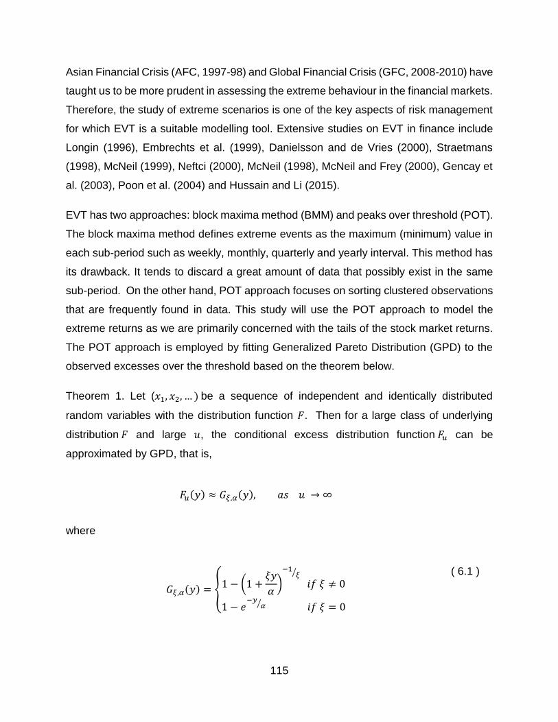
115

Asian Financial Crisis (AFC, 1997-98) and Global Financial Crisis (GFC, 2008-2010) have

taught us to be more prudent in assessing the extreme behaviour in the financial markets.

Therefore, the study of extreme scenarios is one of the key aspects of risk management

for which EVT is a suitable modelling tool. Extensive studies on EVT in finance include

Longin (1996), Embrechts et al. (1999), Danielsson and de Vries (2000), Straetmans

(1998), McNeil (1999), Neftci (2000), McNeil (1998), McNeil and Frey (2000), Gencay et

al. (2003), Poon et al. (2004) and Hussain and Li (2015).

EVT has two approaches: block maxima method (BMM) and peaks over threshold (POT).

The block maxima method defines extreme events as the maximum (minimum) value in

each sub-period such as weekly, monthly, quarterly and yearly interval. This method has

its drawback. It tends to discard a great amount of data that possibly exist in the same

sub-period. On the other hand, POT approach focuses on sorting clustered observations

that are frequently found in data. This study will use the POT approach to model the

extreme returns as we are primarily concerned with the tails of the stock market returns.

The POT approach is employed by fitting Generalized Pareto Distribution (GPD) to the

observed excesses over the threshold based on the theorem below.

Theorem 1. Let (𝑥1, 𝑥2, … ) be a sequence of independent and identically distributed

random variables with the distribution function 𝐹. Then for a large class of underlying

distribution 𝐹 and large 𝑢, the conditional excess distribution function 𝐹𝑢 can be

approximated by GPD, that is,

𝐹𝑢(𝑦) ≈ 𝐺𝜉,𝛼(𝑦), 𝑎𝑠 𝑢 → ∞

where

𝐺𝜉,𝛼(𝑦) = {1 − (1 +

𝜉𝑦

𝛼)

−1𝜉⁄

𝑖𝑓 𝜉 ≠ 0

1 − 𝑒−𝑦

𝛼⁄ 𝑖𝑓 𝜉 = 0

( 6.1 )

116

for 𝑦 ≥ 0 when 𝜉 ≥ 0 and 0 ≤ y ≤ (−𝛼

𝜉) when 𝜉 < 0. α is the scale parameter, 𝜉 is the shape

parameter for the GPD parameters.

For the proof of this theorem, we refer to Balkema and De Haan (1974) and Pickands

(1975).

6.2.2. Copula Models

Copula is a risk management tool that models the dependence structure between

variables and it was first used in finance in the early 2000s (Cherubini et al. 2004).

Specifically, copula is a technique for modelling the dependence structure without the

assumption of normality. It can separate the marginal behaviour of variables from the

dependence structure through the use of joint distribution function.

The traditional linear correlation method does suffer from a few limitations. Zero

correlation does not necessarily mean independence. It also does not work well for

distributions with strong kurtosis. Besides, linear dependent data do not often appear in

finance. Many studies have demonstrated financial dependency are typically nonlinear.

Further, linear correlation only works well if the joint distribution of the variables is elliptical

such as multivariate normal distribution and Student t distribution (Meissner, 2013).

On the other hand, copula does not require the assumption of joint normality and it allows

us to decompose any n-dimensional joint distribution into its n marginal distributions. The

flexibility behind the assumption and the ability to extract information regarding

dependence structure from the joint probability distribution function enable the copula

method to be widely used in various applications. The innovations in copula theory

introduced by Patton (2006a) allow a temporal variation to occur in the conditional

dependence in a time series. This makes copula method more dynamic and time

sensitive. More applications of this method can be found in Bartram et al. (2007), Nguyen

and Bhatti (2012), Wang et al. (2011) among others.

117

Based on Sklar’s theorem (1959), copula values are based on the information of the

marginal distribution that has been transformed into a uniform distribution. The joint

distribution F of r random variables x1, . . ., xr can be decomposed into r marginal

distributions 𝐹1, … , … , . . . , 𝐹𝑟 and C which is known as copula and can be used to describe

the dependence of the structures among the variables:

F (x1 ,…, xr ) = C ( F ( x1 ),……,F( xr )) ( 6.2 )

This study uses bivariate copula for which the above equation for dependence can be

written as:

F (x1,, x2 ) = C ( F ( x1 ),F( x2 )) ( 6.3 )

In this paper, we use both Gaussian and Symmetrized Joe–Clayton (SJC) copula to

examine their effectiveness in modelling the dependence between GCEA stock markets.

Gaussian copula is used as a benchmark for the overall dependence, whereas SJC

copula is used to capture the upper and lower tail dependence simultaneously.

6.3. Methodology

There are two main steps to model the dependence structure between a pair of stock

markets. The first step is to estimate the marginal distribution. The second step is to use

copula model this joint distribution. These twos steps are described below.

6.3.1. Marginal Distribution Estimation

A generalized autoregressive conditional heteroscedastic (GARCH) framework is often

applied to model the volatility of a stock market. In this paper, we apply the GJR-GARCH

model with the assumption of t distribution in the process to discard any serial correlation

and conditional heteroskedasticity process (Engle and Ng, 1993 and Glosten et al., 1993).

118

The t distribution is selected instead of normal distribution because of the strong empirical

evidence in rejecting the concept of normality distribution in financial data.

Let 𝑟𝑖,𝑡 denote returns and ℎ𝑖,𝑡2 denote the conditional variance for the period of 𝑡. The

GJR-GARCH model14 can be formulated as

𝑟𝑡 = 𝜇 + 𝜗𝑟𝑡−1 + 휀𝑡

ℎ𝑡2 = 𝑐 + 𝛾ℎ𝑡−1

2 + 𝜂1휀𝑡−12 + 𝜂2𝑠𝑡−1휀𝑡−1

2

( 6.4 )

( 6.5 )

where 𝑠𝑡−1 = 1 when 휀𝑡−1 is negative and 0 otherwise. The standardize residual of

series, 𝑧𝑡 are modelled as a Student t distribution with 𝑑𝑓 represents the degree of

freedom and Ω t -1 denotes the previous information set:

𝑧𝑡|Ω 𝑡−1 = √𝑑𝑓

𝜎𝑡2(𝑑𝑓 − 2)

휀𝑡𝑧𝑡~𝑖𝑖𝑑 𝑡𝑑𝑓

( 6.6 )

With regard to modelling the (upper and lower) tails of these residuals, the POT method

is applied with a predefined threshold value 𝑢 and the GPD is then used to model the

tails. The process to determine the threshold value 𝑢 is crucial for the GPD modelling.

According to the Picklands–Balkema–De Haan theorem (Balkema and De Haan 1974;

Pickands 1975), a high 𝑢 value is important in order to obtain extreme series. However,

this result generally leads to a large variance in the estimators due to the probability to

discarding the valuable data. Besides, the samples may be too small for data analysis.

The data gathered might not belong to the tails and results in a bias in estimators if the

value of 𝑢 is too low. Thus a trade-off between bias and variance is required to find the

14 Other GARCH models may also be suitable for treating the heteroskedasticity of the returns. GJR-GARCH is commonly used and

thus selected for this study.

119

optimal threshold. Similar to Du and Mouche (1983), 𝑢 is selected as the 90th percentile

for the upper tail the10th percentile for the lower tail in this study.

The cumulative function for this combination (GPD for the tails and the empirical

distribution for the remaining part) can be written as:

𝐹(𝑧) =

{

𝑘𝐿

𝑛(1 + 𝜉

𝑢𝐿 − 𝑧

α)−1

ξ⁄ for 𝑧 < 𝑢𝐿 ,

∅(𝑧) for 𝑢𝐿 < 𝑧 < 𝑢𝑈

1 −𝑘𝑈

𝑛(1 + 𝜉

𝑧 − 𝑢𝑈

α)−1

ξ⁄ for 𝑧 > 𝑢𝑈 ,

( 6.7 )

where α is the scale parameter, 𝜉 is the shape parameter, 𝑢𝐿 (𝑢𝑈) is the lower (upper)

threshold, n is the number of observations, ∅ is the empirical distribution function and

𝑘𝐿(𝑘𝑈) is the number of observations below(exceeding) the threshold 𝑢𝐿 (𝑢𝑈).

6.3.2. Copula Estimation

6.3.2.1. Gaussian Copula

A Gaussian copula is based on a multivariate normal distribution. In the bivariate case,

the random vector 𝑋 = (𝑋1, 𝑋2) is bivariate normal if 𝑋1and 𝑋2 are normal. Therefore the

dependence structure between the margins can be described by the following copula

function:

𝐶(𝑢, 𝑣) = ∫ ∫1

2𝜋√1 − 𝛿2

ᶲ−1(𝑣)

−∞


2(1 − 𝛿2)} 𝑑𝑥𝑑𝑦

ᶲ−1(𝑢)

−∞

= Φ𝛿(Φ−1(𝑢),Φ−1(𝑣)),−1 ≤ 𝛿 ≤ 1

( 6.8 )

( 6.9 )

120

where Φ and Φ𝛿 are the standard normal CDF’s and 𝛿 is the linear correlation coefficient.

6.3.2.2. Symmetrized Joe–Clayton Copula (SJC Copula)

SJC copula is a modified version of the 1997 Joe–Clayton copula. In general, the Joe-

Clayton copula can be defined as:


−1

𝛾 )1/k

( 6.10 )

where

𝑘 =1


𝛾 = −1


( 6.11 )

( 6.12 )

and

𝜏𝑈𝜖( 0 ,1 ), 𝜏𝐿𝜖 (0 , 1 ). ( 6.13 )

However, the original Joe–Clayton copula is not as attractive as SJC copula because SJC

can be symmetric when 𝜏𝑈 = 𝜏𝐿 . Further, SJC copula enables us to capture the lower

and upper tail dependence simultaneously. Thus, SJC copula is the ideal choice for

understanding the tail behaviour of the data (Patton, 2006a) and it can be defined as:


𝑈, 𝜏𝐿) + 𝐶𝐽𝐶(1 − 𝑢, 1 − 𝑣|𝜏𝑈 , 𝜏𝐿) + 𝑢 + 𝑣 − 1] ( 6.14 )

121

where 𝐶𝐽𝐶 is the Joe–Clayton copula and 𝜏𝑈 and 𝜏𝐿 represent upper and lower tail

dependence, respectively.

6.3.3. Dependence Parameters of Dynamic Copula

In this study, Gaussian dependence parameter is assumed to evolve over time according

to the Patton (2006a):

𝛿𝑡 = 𝜆(𝜔 + 𝛽𝛿𝑡−1 + 𝛼1

10∑[Φ−1(𝑢𝑡−𝑗)Φ

−1(𝑣𝑡−𝑗)]

10

𝑗=1

)

( 6.15 )

where 𝜆 = (1 − 𝑒−𝑥)/(1 + 𝑒−𝑥) is the modified logistic transformation which ensures 𝛿𝑡 in

the interval (-1,1) at all times. Note that in Equation (15), an ARMA (1,10) type process

is assumed and 𝛽𝛿𝑡−1 captures the persistence effect and the mean of the product of the

last 10 observations of the transformed variables Φ−1(𝑢𝑡−𝑗) and Φ−1(𝑣𝑡−𝑗) captures the


While according to Patton (2006a), the evolution parameters for the SJC copula can be

defined as:


1

10∑ |𝑢1,𝑡−𝑖 − 𝑢2,𝑡−𝑖|

10

𝑖=1)

( 6.16 )

where �̃� is given as the logistic transformation: �̃�(𝑥) = (1 + 𝑒−𝑥)−1, which ensures the

dependence parameter 𝜏𝑈/𝐿 in (0,1).

122

6.3.4. Estimation Method

6.3.4.1. Marginal Estimation

The Maximum Likelihood Estimation (MLE) method is used for estimating the parameters.

Based on (7), the full estimation of the combination parametric and GPD distribution can

be written as:

�̂�(𝑧) =

{

𝑘𝐿

𝑛(1 + 𝜉

𝑢𝐿 − 𝑧

α̂)−1

ξ̂⁄ for 𝑧 < 𝑢𝐿 ,

1 −𝑘𝑈

𝑛(1 + 𝜉

𝑧 − 𝑢𝑈

α̂)−1

ξ̂⁄ for 𝑧 > 𝑢𝑈 ,

( 6.17 )

where α̂ and 𝜉 denote the MLE of α and 𝜉, respectively.

6.3.4.2. The Inference Functions of Margins (IFM) for Copula

Copula parameters are estimated by using IFM method rather than MLE method mainly

due to the consideration of computation time and complexity. Moreover, it has advantage

of assessing the goodness of fit of the margin separately. IFM method has two main steps

as follows.

Step 1 : MLE is used to estimate the parameters of marginal distribution according to :

𝜃𝑖 = arg𝑚𝑎𝑥𝑙𝑐(𝜃𝑖) = arg𝑚𝑎𝑥∑𝑙𝑜𝑔𝑓𝑖(𝑥𝑖, 𝜃𝑖)

𝑇

𝑡=1

( 6.18 )

where 𝑙𝑐 is the log-likelihood function of the marginal distribution Fi.

Step 2 : Based on the 𝜃𝑖 , the copula parameters 𝛿 are estimated:

123

𝛿 = arg𝑚𝑎𝑥𝑙𝑐(𝛿) = arg𝑚𝑎𝑥∑log (𝑐(𝐹1(𝑥1, 𝜃1),… , 𝐹𝑛(𝑥𝑛, 𝜃𝑛); 𝛿))

𝑇

𝑡=1

( 6.19 )

where 𝑙𝑐 is the likelihood function of the copula. The estimators are consistent under

standard regularity conditions.

6.3.5. Model Selection Criteria

There are many goodness of fit tests which can be used to identify a suitable model

(Fermanian 2005; Chen and Fan 2006; Hans 2007). In this study, we use Akaike

Information Criterion (AIC) and Bayesian Information Criterion (BIC) which are derived

from information theory. They are widely used to determine the best type of copula.

AIC works based on the trade-off between complexities and information lost when a given

model is used to represent the process that generates data. AIC can be defined as

AIC = −2 log( likelihood )+2k ( 6.20 )

where k is the number of parameters used in the model. The value is a measure based

on the relative distance between the unknown true likelihood function of the data and the

fitted likelihood function of the model. Therefore, a lower AIC means a model is closer to

the truth.

Bayesian Information Criterion (BIC) is defined as

BIC = −2 log( likelihood )+k·log(n) ( 6.21 )

where n is the number of data and k is the number of parameters used in the model. BIC

works similarly as AIC test, but it penalizes model complexity more heavily. The best one

that fits the model is the one with the lowest BIC.

124

6.4. Data and Descriptive Statistics

In this study, we use Shanghai Composite Index for SHSE and Shenzhen Composite

Index for SZSE, Hang Seng Index for HKSE and Taiwan Stock Exchange Weighted Index

for TWSE. The daily closing prices from 1 January 2000 to 31 December 2013 were

obtained from Datastream. Daily logarithmic returns can be defined as rt = ln P t – ln Pt−1

, where Pt is the closing price of the index at time t in our study.

Figure 6.1. Relative daily index level

The sample consists of 13 years of daily data with 3651 observations. This period has

witnessed a few of financial crises such as the Global Financial Crisis (GFC) and

European Debt Crisis. The GFC that erupted in 2008 is considered by many as the worst

financial crisis in history and it has an enormous impact on the GCEA. However, the

European Debt Crisis had limited impact on the GCEA. Thus we will consider the GFC

effect on dependence structure among the GCEA stock markets.

Figure 6.1 presents the relative index level series of GCEA stock markets for the whole

sample period. It is clear that the series of SHSE and SZSE have an upward trend from

2006 to 2008. The same trend is also evident for the HKSE and TWSE. Both show an

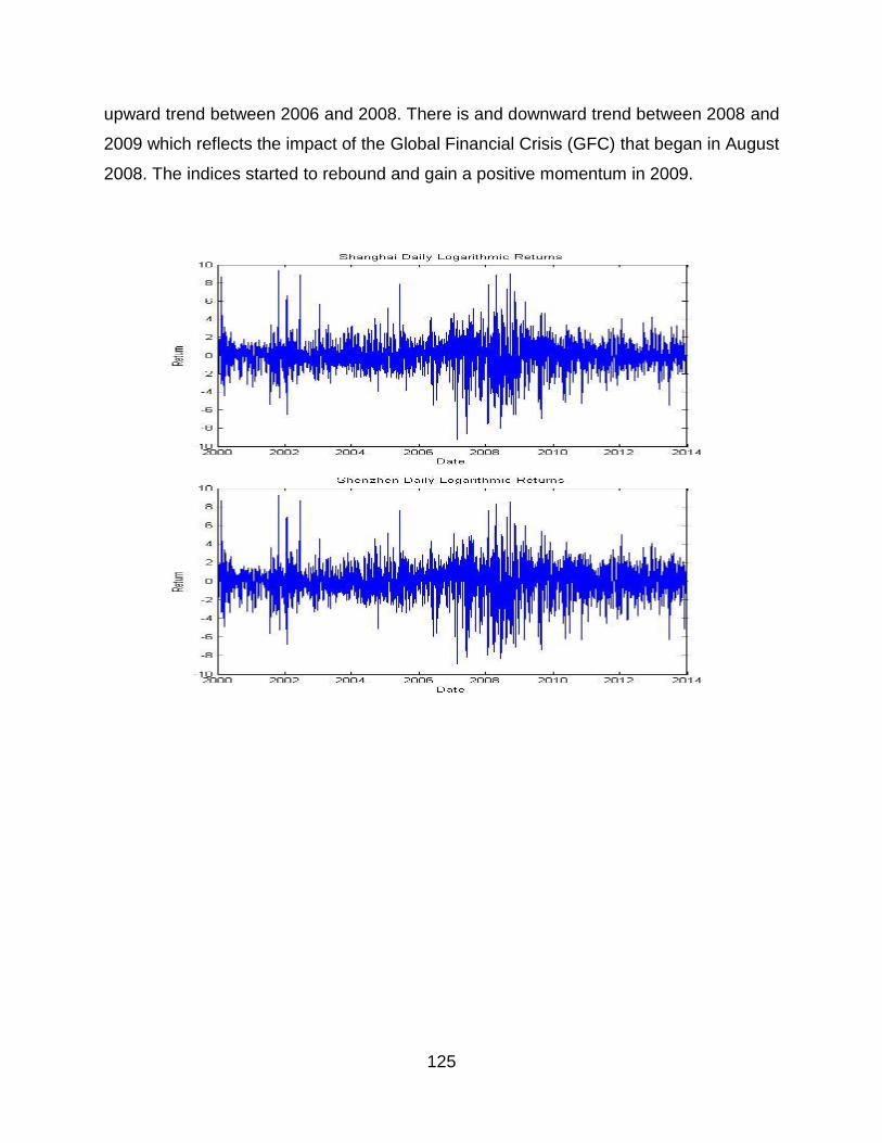
125

upward trend between 2006 and 2008. There is and downward trend between 2008 and

2009 which reflects the impact of the Global Financial Crisis (GFC) that began in August

2008. The indices started to rebound and gain a positive momentum in 2009.

126

Figure 6.2. Daily returns for GCEA stock markets

Figure 6.2 depict the daily logarithmic returns for the GCEA stock markets. It clearly

shows that all the stock markets under consideration are more volatile during the GFC

period. Moreover, as expected, the figure also shows that SHSE and SZSE are more

closely related in terms of volatility.

127

Table 6.1. Descriptive statistics of daily returns

SHSE SZSE HKSE TWSE

No. Obs. 3651 3651 3651 3651

Mean 0.0120 0.0265 0.0081 0.0005

Median 0.0000 0.0118 0.0000 0.0000

Min -9.2561 -8.9303 -13.5820 -9.9360

Max 9.4010 9.2436 13.4068 6.5246

Std 0.0256 1.6915 0.0256 0.0242

Skew -0.0896 -0.3725 -0.0675 -0.2295

Kurtosis 4.7693 3.5930 8.2963 3.0351

JB Sta (p-value) 3453.3530(0.0000) 2041.1310(0.0000) 10440.4200(0.0000) 1428.025(0.0000)

Mean, Med, Min, Max, Std, Skew and Kurt stand for the mean, median, minimum, maximum, the standard deviation, skewness and kurtosis for each series, respectively. JB sta denotes the statistic for the Jarque-Bera normality test with two degrees of freedom.

Table 6.1 reports the descriptive statistics of daily returns for the GCEA stock market. A

few observations can be made. All the series have positive means. SZSE has the highest

mean with 0.0265% followed by SHSE with 0.0120%. TWSE has the lowest mean

(0.0005%). The median for all series is 0.0000% except for SZSE. HKSE has the lowest

minimum (-13.5820%). HKSE also has the highest maximum return (13.4068%). The

standard deviation measure shows that SZSE has the highest volatility (1.6915) while

TWSE has the lowest volatility. This indicates SZSE is most volatile among the four

markets. All the series are skewed to the left. HKSE has the highest value of skewness

and SZSE has the lowest skewness. Finally, HKSE has the highest Kurtosis value

(8.2963) and TWSE has the lowest Kurtosis value (3.0351). Thus the return distributions

of the four markets are all leptokurtic.

Looking at Jarque Bera statistics, HKSE has the highest value and TWSE has the lowest

value. The Jarque Bera test results strongly reject the normal distribution for all return

128

series. All series exhibit a nonlinear phenomenon and extreme behaviour. The normality

assumption is not valid for all series. Thus the EVT approach seems to be a valid choice.

Table 6.2. Linear correlations between markets

SHSE SZSE HKSE TWSE

SHSE 1

SZSE 0.9324 1

HKSE 0.3516 0.3013 1

TWSE 0.1861 0.1583 0.4751 1

Table 6.2 reports the returns correlation among the series. The strongest correlation is

exhibited between SHSE and SZSE. This is an expected outcome because both are

located in mainland China. The second highest correlation is between HKSE and TWSE.

The weakest correlation is between SZSE and TWSE. These figures show the strength

of overall dependence among the GCEA stock markets. However, there is no information

content regarding the tail dependence.


In this section, we present the empirical results of this study. First, we consider the

estimation of the marginal models. Second, we discuss the estimation of the copula

models; Third, the GFC effect is analysed.

6.5.1. Estimating Marginal Models

In this paper, EVT approach is employed to model the tail distributions for every index

series. The top and bottom 10% of the residuals are used for modelling the upper and

129

lower tails, respectively. These residuals are obtained as described in Section 6.3.1. GPD

is used to fit these residuals. The values of the parameters obtained using GPD for the

upper and lower tails are presented in Table 6.3.

Table 6.3. The parameter tails fitted by GPD

SHSE SZSE HKSE TWSE

Lower tail

𝜉 -0.0101 -0.0189 0.0093 0.0282

α 0.6599 0.7132 0.5805 0.6128

Upper tail

𝜉 0.1026 0.0903 -0.1719 -0.1179

α 0.5217 0.4602 0.6182 0.5514

Notes: This table represents estimated parameters between selected stock markets using Generalized Pareto Distribution (GPD). 𝜉 represents the shape and α is the value of the scale parameter of the fitted GPD.

Table 6.3 summarizes the parameter estimates for the lower and upper tails based GPD.

First look at the lower tails. Clearly, TWSE exhibits the strongest heavy tail as it has the

highest absolute value of 𝜉. It is followed by SZSE with 𝜉 =0.0189. HKSE has the lowest

absolute value for the 𝜉, thus its lower tail is not so heavy.

Now turn to the upper tails. The values of 𝜉 are positive for SHSE and SZSE, and negative

for both HKSE and TWSE. The estimates indicate that HKSE and TWSE have heavy

upper tails (𝜉 =0.1719, 0.1179 for HKSE and TWSE, respectively). In contrast, the upper

tails for SHSE and SZSE are not so heavy.In summary, TWSE has heavy tails on both

sides. This means that the TWSE is more volatile than other ones in terms of upside and

downside risks. Further, let us compare SHSE with SZSE. The 𝜉 estimates indicate SZSE

has a stronger heavy lower tail than SHSE, whereas SHSE has a stronger heavy upper

tail than SZSE.

130

To visually assess the GPD fit, we plot the empirical CDF of the upper (lower) tail

exceedances of the residuals along with CDF by the GPD in Figure 6.3 (6.4). Although

only 10% of the standardized residuals is used, the fitted distribution closely follows the

exceedance data. Thus GPD model seems to be a good choice for both tails.

The overall marginal distributions used in this study are shown in Figures 6.5. The tails

are fitted by using EVT while the central part is estimated by a Gaussian kernel. This

smooths the CDF estimates, eliminating the staircase pattern of unsmoothed sample

CDFs. The non-parametric method kernel CDF is well suited for the interior of the

distribution where most of the data is found. However, this method tends to perform poorly

when applied to the upper and lower tails. The combination with EVT for the tails can

overcome this problem.

In summary, Figures 6.3, 6.4 and 6.5 demonstrate that our approach can adequately

model the marginal distributions of all data series.

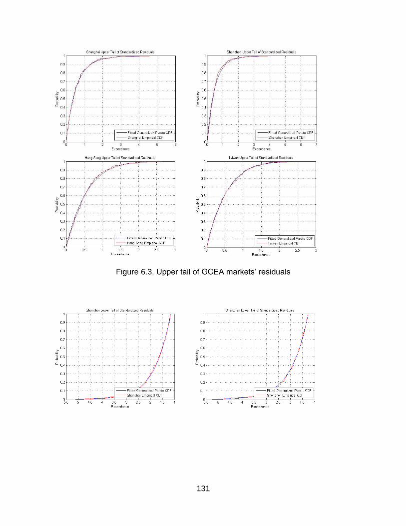
131

Figure 6.3. Upper tail of GCEA markets’ residuals

132

Figure 6.4. Lower tail of GCEA markets’ residuals

Figure 6.5. Fitting residuals for the GCEA stock markets

133

6.5.2. Estimating the Copula Models

In this paper, we are interested in the behaviour of extreme returns. Thus we use copula

functions which specifically focus on the tails. To this end, Gaussian and SJC copula are

considered. The SJC copula has the advantage of allowing different parameters for the

lower and upper tails and thus takes the difference in the behaviour of the upper and

lower tails into account. In this paper, the dependence parameters (for Gaussian and

SJC) are assumed to follow Patton equation (Patton 2006a).

Table 6.4 presents the parameter estimates for the Gaussian and SJC copulas. For the

constant copulas, the key parameters are 𝛿 (Gaussian), 𝜏𝑈 and 𝜏𝐿 (SJC). For the

dynamic copulas, we focus on 𝜔 (Gaussian), 𝜔𝑈 and 𝜔𝐿 (SJC) which are used as a

measure of the dependence level of each pair of stock markets. The adjustment in the

dependence is captured by 𝛼𝑈 (Gaussian), 𝛼𝑈 and 𝛼𝐿 (SJC). The degree of persistence

of dependence is represented by parameter 𝛽 (Gaussian), 𝛽𝑈 and 𝛽𝐿 (SJC). The values

for the AIC and BIC are used as goodness of fit measure. A lower AIC or BIC value

indicate a better fit.

Figure 6.6 represents the time evolution of the dependence parameters of each pair of

GCEA stock markets.

134

Table 6.4. Parameter estimates for constant and dynamic copulas15

SHSE-SZSE

SHSE-HKSE SHSE-TWSE

SZSE-HKSE

SZSE-TWSE

HKSE-TWSE

Gaussian Copula

δ 0.9276*** 0.3094*** 0.1898*** 0.261*** 0.1635*** 0.4901***

AIC -7188.7 -367.279 -133.9235 -257.6178 -98.869 -1002.7202

BIC -7188.7 -367.2773 -133.9218 -257.6161 -98.8673 -1002.7185

SJC Copula

𝜏𝑈 0.7920*** 0.0976*** 0.0012 0.0706*** 0.0037 0.2773***

𝜏𝐿 0.8337*** 0.1789*** 0.1216*** 0.1295*** 0.0772*** 0.3220***

AIC -

7504.2526 -385.0091 -158.8489 -271.1503 -111.1265 -1026.5926

BIC -

7491.8471 -372.6036 -146.4433 -258.7448 -98.721 -1014.1871

Dynamic Gaussian Copula

ω -8.1017*** 0.0136* 0.0034* 0.0083 0.0003 0.1197

α 0.0231*** 0.125*** 0.0527*** 0.0794** 0.0196*** 0.1843***

β 12.2696*** 1.9505*** 1.9785*** 1.9709*** 2.0066*** 1.8057***

AIC -7194 -474.0517 -188.7604 -314.8249 -129.1187 -1054.7051

BIC -7194 -474.0466 -188.7553 -314.8198 -129.1136 -1054.7

Dynamic SJC Copula

15 Matlab is used in the calculations of copula parameters .The authors would like to thank Manthos Vogiatzoglou from the and Osvaldo Silva for their help.

135

𝜔𝑈 1.2891** 0.076* -9.5043*** 0.0931*** -4.8826 0.3105***

𝛼𝑈 -0.3347 -0.3766* -9.9942*** -0.4012*** -1.1221 -1.7004***

𝛽𝑈 -4.0354*** 0.99*** 10.0000*** 0.9932*** 3.2603 0.8772***

ωL 1.3821** 0.1141** 0.0985*** 0.0591 0.1527 0.1572***

𝛼𝐿 -0.3202*** -0.5343** -0.4372*** -5.4625* -0.8053 -0.7517***

𝛽𝐿 -4.2186** 0.9812*** 0.9865*** 0.1500 0.9654*** 0.9530***

AIC -

3910.2329 -501.7875 -190.5665 -302.789 -123.5252 -1121.3555

BIC -

3873.0164 -464.571 -153.3499 -265.5728 -86.3086 -1084.139

Notes:δ is the parameter of Gaussian copula. τU and τL are the upper and lower tails of the SJC copula;ω is constant: α and β are the coefficients of the dynamic process proposed. AIC and BIC are Akaike and Bayesian Information Criteria.* = P<0.1, ** = P<0.05 and *** = P<0.01.

SHSE-SZSE

136

SHSE-HKSE

SHSE-TWSE

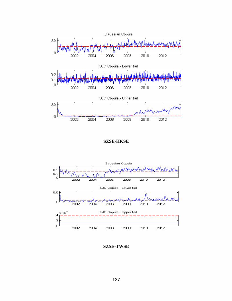
137

SZSE-HKSE

SZSE-TWSE

138

HKSE-TWSE

Figure 6.6. Evolution of the dependence parameters

Notes : In each graph, the dashed line denote the dependence parameter for the constant copula while the solid curve denotes

the parameter values under the dynamic copula.

6.5.2.1. Constant Copula Models

A few observations can be made from Table 6.4 and Figure 6.6. According to results for

the constant Gaussian copula model, the overall dependence among the 6 pairs of stock

markets can be ranked in a decreasing order as: SHSE-SZSE > HKSE-TWSE > SHSE-

HKSE > SZSE-HKSE > SHSE-TWSE >SZSE-TWSE. According to the results for the SJC

copula, the upper tail dependence among the 6 pairs of stock markets can be ranked in

a decreasing order as: SHSE-SZSE > HKSE-TWSE > SHSE-HKSE > SZSE-HKSE >

SZSE-TWSE > SHSE-TWSE; the lower tail dependence among the 6 pairs of stock

markets can be ranked in a decreasing order as: SHSE-SZSE > HKSE-TWSE > SHSE-

HKSE > SZSE-HKSE > SHSE-TWSE >SZSE-TWSE. These facts clearly indicate that

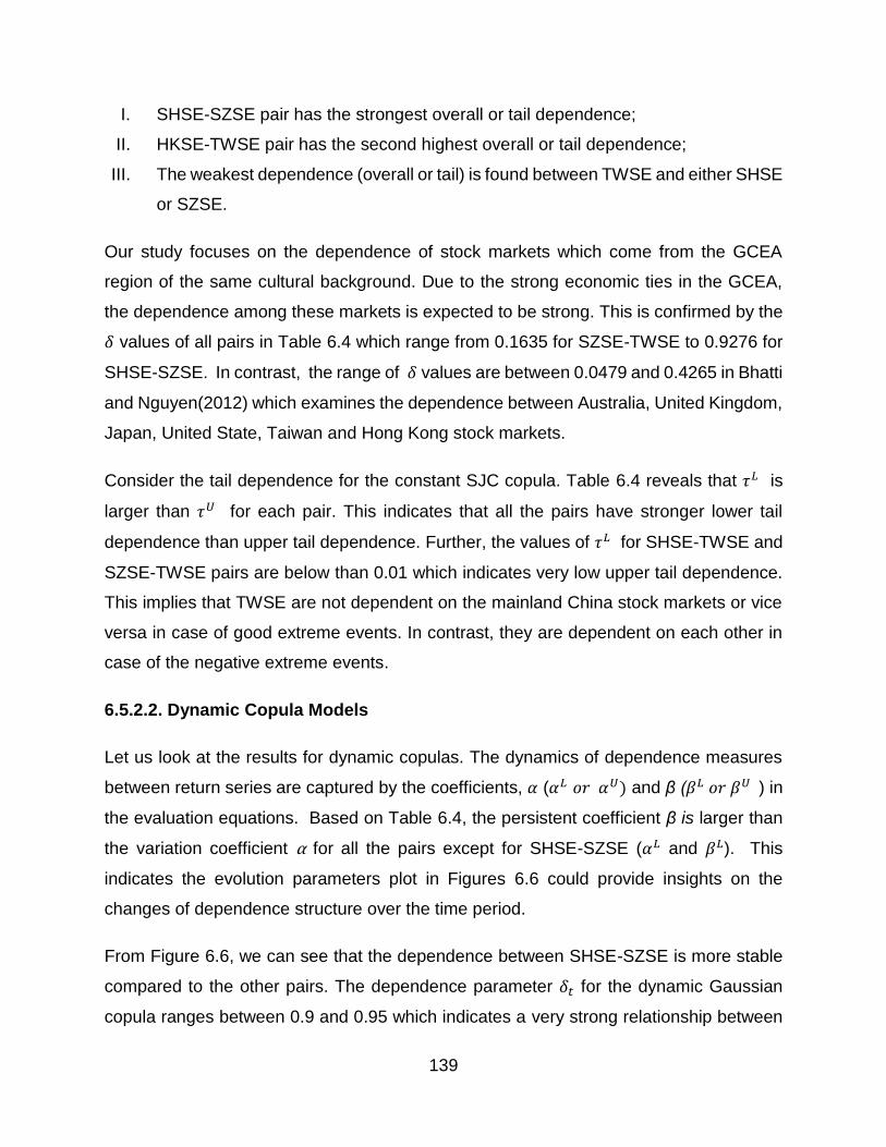
139

I. SHSE-SZSE pair has the strongest overall or tail dependence;

II. HKSE-TWSE pair has the second highest overall or tail dependence;

III. The weakest dependence (overall or tail) is found between TWSE and either SHSE

or SZSE.

Our study focuses on the dependence of stock markets which come from the GCEA

region of the same cultural background. Due to the strong economic ties in the GCEA,

the dependence among these markets is expected to be strong. This is confirmed by the

𝛿 values of all pairs in Table 6.4 which range from 0.1635 for SZSE-TWSE to 0.9276 for

SHSE-SZSE. In contrast, the range of 𝛿 values are between 0.0479 and 0.4265 in Bhatti

and Nguyen(2012) which examines the dependence between Australia, United Kingdom,

Japan, United State, Taiwan and Hong Kong stock markets.

Consider the tail dependence for the constant SJC copula. Table 6.4 reveals that 𝜏𝐿 is

larger than 𝜏𝑈 for each pair. This indicates that all the pairs have stronger lower tail

dependence than upper tail dependence. Further, the values of 𝜏𝐿 for SHSE-TWSE and

SZSE-TWSE pairs are below than 0.01 which indicates very low upper tail dependence.

This implies that TWSE are not dependent on the mainland China stock markets or vice

versa in case of good extreme events. In contrast, they are dependent on each other in

case of the negative extreme events.

6.5.2.2. Dynamic Copula Models

Let us look at the results for dynamic copulas. The dynamics of dependence measures

between return series are captured by the coefficients, 𝛼 (𝛼𝐿 𝑜𝑟 𝛼𝑈) and β (𝛽𝐿 𝑜𝑟 𝛽𝑈 ) in

the evaluation equations. Based on Table 6.4, the persistent coefficient β is larger than

the variation coefficient α for all the pairs except for SHSE-SZSE (𝛼𝐿 and 𝛽𝐿). This

indicates the evolution parameters plot in Figures 6.6 could provide insights on the

changes of dependence structure over the time period.

From Figure 6.6, we can see that the dependence between SHSE-SZSE is more stable

compared to the other pairs. The dependence parameter 𝛿𝑡 for the dynamic Gaussian

copula ranges between 0.9 and 0.95 which indicates a very strong relationship between

140

the two stock markets. Further, with the dynamic SJC copula, 𝜏𝑈 and 𝜏𝐿 are around 0.8

and 0.7, respectively. This indicates strong upper and lower tail dependence bewteen

these two markets. In sum, SHSE-SZSE pair has the strongest dependence as confirmed

above.

For the SHSE-HKSE, the values of dependence parameter 𝛿𝑡 in the dynamic Gaussian

copula are between 0 and 0.3 before 2007, and it is between 0.3 and 0.5 after 2007. A

similar change around 2007 can be observed for the parameters 𝜏𝑈 and 𝜏𝐿 in the dynamic

SJC copula.

For the SHSE-TWSE pair, Figure 6.6 reveals that the values of the dependence

parameter 𝛿𝑡 before 2007 are quite volatile ranging between 0 and 0.3, whereas the

values after 2007 are more stable fluctuating around 0.4.The lower tail dependence

parameter 𝜏𝐿 for this pair has an upward trend since 2007. The parameter 𝜏𝑈 for this pair

is almost zero which indicates there is hardly any dependence between these two

markets in the case of positive extreme events.

For the SZSE-HKSE pair, the dependence structure is quite revealing in several ways.

Similarly to the SHSE-TWSE pair, Figure 6.6 reveals that the values of the dependence


values after 2007 are more stable fluctuating around 0.4. However, the lower tail

dependence parameter 𝜏𝐿 for this pair is stable and ranging between 0.1 and 0.2. The

upper tail dependence parameter 𝜏𝑈 has an upward trend since 2009.

For the SZSE-TWSE pair, Figure 6.6 reveals that the values of the dependence


values after 2007 are more stable fluctuating around 0.25. However, the lower tail

dependence parameter 𝜏𝐿 for this pair is stable except a peak around 2010. The

parameter 𝜏𝑈 for this pair is almost zero which indicates there is hardly any dependence

between these two markets in the case of positive extreme events.

Finally, let us consider the HKSE-TWSE pair. Figure 6.6 reveals that the values of the

dependence parameter 𝛿𝑡 are quite stable ranging between 0.4 and 0.55. The tail

141

dependence parameters 𝜏 𝐿 and 𝜏 𝑈 for this pair are also stable between 2002 and 2010.

Thus the dependence structure between this pair was not affected by the GFC.

Next, we explore the information regarding the relative strength of upper and lower tail

dependence. These values could be used to identify the diversification opportunity that

might exist. Table 6.4 shows that 𝜔𝐿 is bigger than 𝜔𝑈 for most paris except two pairs

(SZSE and HKSE, HKSE and TWSE). Thus the lower tail dependence is relatively higher

for these pairs. When market is down, the risk diversification is less effective becaue of

this greater dependence for these pairs. Similarly, when market is down, the risk

diversification is more effective for the two pairs: SZSE and HKSE, HKSE and TWSE.

Investors who invest in HKSE might consider SZSE or TWSE to be their preferred choice

for managing the downside risk. These results are not in line with the linear correlation

reported in Table 6.2 which implies that SZSE-TWSE pair is the best choice for

diversification purpose in the mean-variance setting. This may be due to the normality

assumption associated with the linear correlation approach. Thus the copula method

provides more information compared to the linear correlation. It can provide better insight

to portfolios diversification (Wang et al., 2011). This significantly demonstrates the

advantages of using copula compared to linear correlation.

Finally, it is worth noting the goodness of fit results. According to Table 6.4, dynamic

copulas (Gaussian or SJC) generally fit the data better than the constant copulas. One

exception is a SHSE-SZSE pair for which the constant SJC copula yields the best fit due

to the high correlation between them. For other pairs, dynamic Gaussian copula is the

best fit for two pairs (SZSE-HKSE and SZSE-TWSE) while the dynamic SJC is the best

fit for three pairs (SHSE-HKSE, SHSE-TWSE, and HKSE-TWSE). The results are

summarised in Table 6.5 below.

142

Table 6.5. Model comparison: constant vs. dynamic copulas

SHSE-SZSE SHSE-HKSE SHSE-TWSE SZSE-HKSE SZSE-TWSE HKSE-TWSE

Gaussian Copula

Constant

Dynamic X X X X* X* X

SJC Copula

Constant X*

Dynamic X* X* X X X*

X indicates the better fit model among the constant and dynamic copula for each type of copula. X* indicates the best fit model among all 4 constant and dynamic copula models.

In summary, the empirical findings on dynamic copula models can improve our

understanding of the dependence among GCEA markets and help in considering portfolio

allocation and risk management strategy.

6.5.2.3. GFC effect

Based on the literature, the dependence structure between markets tends to be greater

during a financial crisis. GFC is a major event in the sample period and it is natural that

we consider GFC effect on the GCEA stock markets. Figure 6 shows that the dependence

structure for most of the pairs of stock markets started to increase during 2007 when the

GFC started. Thus the dynamic copula models appear to have some prediction power on

the GFC.

There is no evident GFC effect on the dependence (overall, lower tail or upper tail)

between two pairs, namely, SHSE-SZSE and HKSE-TWSE. SHSE-SZSE are highly

dependent on each other with values of 𝛿𝑡 fluctuating between 0.9 and 0.95. The

dependence between HKSE-TWSE is highly stable with 𝛿𝑡 fluctuating around 0.5. Thus

the dependence structure is strong and mature for these two pairs and thus not affected

by GFC.

143

Next, consider the dependence structure for the other 4 remaining pairs. Figure 6.6

shows the overall dependence structure changes and the overall dependence becomes

stronger after 2007 for the remaining four pairs. With respect to the lower tail dependence,

it becomes stronger for the SHSE related pairs and there is no evident GFC effect for the

SZSE related pairs. With respect to the upper tail dependence, it becomes stronger for

the HKSE related pairs and there is no evident GFC effect for the TWSE related pairs.

It can also be observed that the lower tail dependence is stronger than the upper tail

dependence during GFC for all pairs of stock markets considered. This observation is in

the same vein as the findings in the literature with other markets.

Finally, it should be notated that the dependence between most of the pairs of stock

markets remains strong in the post-GFC period. Thus, the regime for the dynamic

dependence structure between most pairs of stock markets appears to have changed as

a result of the GFC.

6.6. Concluding remarks

Over the past few years, there have been a lot of interests in the research on the

dependence between financial markets by using the copula approach. Until now, little is

known about the dependence structure between GCEA markets despite their importance.

This study examines the dynamic dependence of the GCEA markets using dynamic

copula and EVT.

EVT is good for modelling tail behaviour. We thus use EVT to estimate all the marginal

distributions. We then use Gaussian and SJC copula models to assess the dependence

structure between each pair of the stock markets. In this study, copula parameters are

allowed to vary over time and follow ARMA-type evolution equations. Gaussian copula is

used as a benchmark for comparison. SJC copula is used to capture the upper and lower

tail dependence of the return series.

144

This study reveals that the SHSE-SZSE pair, followed by HKSE-TWSE, has the strongest

overall or tail dependence among all pairs. The weakest dependence (overall or tail) is

found between TWSE and either SHSE or SZSE. Further, we note that the upper tail

dependence between two TWSE related pairs ( SHSE-TWSE and SZSE-TWSE) is very

low. This implies that at booming times, TWSE does not has much dependence with the

stock markets in mainland China. In contrast, HKSE does have significant dependence

with the stock markets in mainland China at booming times. Thus it appears that HKSE

is more closely related to the stock markets in mainland China at booming times than

TWSE. This may be due to the dual listing of many mainland stocks in the HKSE rather

than the TWSE.

The risk diversification is more effective for SZSE-HKSE pair as well as HKSE-TWSE

pair than other pairs when the market is down. To the best of our knowledge, this outcome

has not been previously documented in the literature.

Overall, we obtain more information regarding the dependence structure by using the SJC

copula than using the linear correlation. This study thus provides evidence supporting

that the combination of Copula and EVT can be a promising method to understand the

dependence structure.

Finally, we note that further research can be pursued in the vein of this paper. For

example, the combination of the dynamic copula model and EVT used in this paper can

be useful in computing Value at Risk (VaR). Moreover, the reasons for the dependence

results obtained in the paper can be further investigated.

145

6.7. References

Aggarwal, R., Inclan, C. and Leal, R., 1999. Volatility in emerging stock markets. Journal

of Financial and Quantitative Analysis, 34(01), pp.33-55.

Ané, T and Labidi, C 2006, 'Spillover effects and conditional dependence', International

Review of Economics and Finance, vol. 15, no. 4, pp. 417-42.

Balkema, AA and De Haan, L 1974, 'Residual life time at great age', Annals of Probability,

vol. 2, no. 5, pp. 792-804.

Bartram, SM, Taylor, SJ and Wang, YH 2007, 'The Euro and European financial market


Bhatti, MI and Nguyen, CC 2012, 'Diversification evidence from international equity

markets using extreme values and stochastic copulas', Journal of International

Financial Markets, Institutions and Money, vol. 22, no. 3, pp. 622-46.

Chen, X and Fan, Y 2006, 'Estimation of copula-based semiparametric time series

models', Journal of Econometrics, vol. 130, no. 2, pp. 307-35.

Cheng, H and Glascock, JL 2005, 'Dynamic linkages between the greater China

economic area stock markets—Mainland China, Hong Kong, and Taiwan', Review

of Quantitative Finance and Accounting, vol. 24, no. 4, pp. 343-57.

Cherubini, U, Luciano, E and Vecchiato, W 2004, Copula methods in finance, John Wiley

& Sons.

Cheung, Y-W, Chinn, MD and Fujii, E 2003, 'China, Hong Kong, and Taiwan: A

quantitative assessment of real and financial integration', China Economic Review,

vol. 14, no. 3, pp. 281-303.

Cheung, YW, Chinn, MD and Fujii, E 2005, 'Dimensions of financial integration in greater



146

Danielsson, J and de Vries, CG 2000, 'Value-at-risk and extreme returns', Annales


DuMouchel, W. H. (1983). Estimating the stable index α in order to measure tail thickness:

a critique. the Annals of Statistics, 1019-1031.

Embrechts, P, Lindskog, F and McNeil, A 2001, 'Modelling dependence with copulas and

applications to risk management', Modelling Dependence with Copulas and

Applications to Risk Management.

Embrechts, P, Resnick, SI and Samorodnitsky, G 1999, 'Extreme value theory as a risk


Engle, RF and Ng, VK 1993, 'Measuring and testing the impact of news on volatility', The


Fermanian, JD 2005, 'Goodness-of-fit tests for copulas', Journal of Multivariate Analysis,

vol. 95, no. 1, pp. 119-52.

Fisher, RA and Tippett, LHC 1928, 'Limiting forms of the frequency distribution of the

largest or smallest member of a sample', paper presented to Mathematical

Proceedings of the Cambridge Philosophical Society.

Forbes, KJ and Rigobon, R 2002, 'No contagion, only interdependence: Measuring stock

market comovements', Journal of Finance, vol. 57, no. 5, pp. 2223-61.

Gençay, R, Selçuk, F and Ulugülyaǧci, A 2003, 'High volatility, thick tails and extreme

value theory in value-at-risk estimation', Insurance: Mathematics and Economics,

vol. 33, no. 2, pp. 337-56.

Glosten, LR, Jagannathan, R and Runkle, DE 1993, 'On the relation between the

expected value and the volatility of the nominal excess return on stocks', The


147

Hans, M 2007, 'Estimation and model selection of copulas with an application to exchange

rate', Estimation and model selection of copulas with an application to exchange

rate.



83.

Hussain, SI and Li, S 2015, 'Modeling the distribution of extreme returns in the Chinese

stock market', Journal of International Financial Markets, Institutions and Money,

vol. 34, no. 0, pp. 263-76.

Hyde, S, Bredin, D and Nguyen, N 2007, Chapter 3 Correlation dynamics between Asia-


Johansson, AC and Ljungwall, C 2009, 'Spillover effects among the greater China stock


Jondeau, E and Rockinger, M 2006, 'The Copula-GARCH model of conditional





Longin, F and Solnik, B 2001, 'Extreme correlation of international equity markets',


Longin, FM 1996, 'The asymptotic distribution of extreme stock market returns', Journal





148

McNeil, AJ1999, 'Extreme value theory for risk managers', Extreme Value Theory for Risk

Managers.



7, no. 3-4, pp. 271-300.

Meissner, G 2013, Correlation Risk Modeling and Management: An Applied Guide

including the Basel III Correlation Framework - With Interactive Models in Excel /

VBA, Wiley.



Nguyen, CC and Bhatti, MI 2012, 'Copula model dependency between oil prices and stock









Poon, SH, Rockinger, M and Tawn, J 2004, 'Extreme value dependence in financial


Studies, vol. 17, no. 2, pp. 581-610.

Rodriguez, JC 2007, 'Measuring financial contagion: A Copula approach', Journal of


149

Shin, K and Sohn, CH 2006, 'Trade and Financial Integration in East Asia: Effects on Co‐



8.



Wang, K, Chen, Y-H and Huang, S-W 2011, 'The dynamic dependence between the

Chinese market and other international stock markets: A time-varying copula

approach', International Review of Economics & Finance, vol. 20, no. 4, pp. 654-64.

Wang, Y and Iorio, AD 2007, 'Are the China-related stock markets segmented with both



Xu, XE and Fung, HG 2002, 'Information flows across markets: evidence from China–

backed stocks dual–listed in Hong Kong and New York', Financial review, vol. 37,

no. 4, pp. 563-88.

150

CHAPTER 7: SUMMARY AND

CONCLUDING REMARKS

7.1. Main Findings

A study on the Chinese stock market by using EVT and copula is carried out in this thesis.

Some major conclusions can be summarised as follows.

In Chapter 4, we investigate the distribution of the extreme returns in the Chinese stock

market.Specifically, the best distributions that fit with the extreme returns of the Chinese

stock market for the minima and maxima series are explored in depth. This approach is

expected to yield better results for computing VaR or the expected shortfall than the

traditional methods based on normal assumption.

Traditionally, normal distribution has been used to model the extreme returns. The misuse

of distribution can lead to underestimating the financial risk based on measures such as

VaR.

There are three main distributions often used in EVT: GEV, GL and GP distribution. Most

literature concerning EVT tends to focus on the GEV distribution. In contrast to what has

been published, this study shows that the GL distribution is the best fit for the Minima

series while the GEV distributes the best fit for the maxima series for the Chinese stock

market.

A robust test is carried out by considering the price restriction and GFC. It is found that

the result remains the same regardless of the events. This finding can have an impact on

the application and measurement of risk management.

Chapter 5 reveals that China-Australia stock market pair has the strongest overall

dependence, followed by the China-Japan pair. The Chinese stock market seems to have

151

a greater dependence on Australian stock market compared to Japanese stock market.

It is also found that the dependence for the upper tails is low for the China-US and China-

UK pairs. This indicates that the Chinese stock market is not much affected by the UK or

US or vice versa in the case of positive extreme events. In contrast, these pairs seem to

have more dependence in the case of negative extreme events. This implies that the

Chinese stock market will have more impact on these stock markets in a burst than a

boom.

As we compared between continents, the dependence of the Chinese stock market with

the UK or Germany is almost double that of the US. This indicates the Chinese stock

market has greater dependence on the European stock markets than the US stock

market. The Canadian stock market seems to have more dependence on the Chinese

stock market compared to the US stock market. There are many reasons for these

empirical results. From the economic perspective, China is the largest exporter of goods

in the world. It has created a huge demand for commodity products and consequently has

generated huge export booms in many markets and especially Australia.

This study also demonstrated that the dependence for these pairs is much stronger during

a crisis compared to a normal period. Therefore, portfolio diversification across these

pairs will not lead to many benefits during a crisis. Furthermore the empirical results show

the time-varying copula perform better than constant copula. The evidence of this study

suggests that the information gathering from time-varying copula also is more useful than

constant copula. This method provides us important information regarding the time path

of dependence. As we can see, there is a stable and volatile time path. These findings

indicate the regimes of time path might change during a certain period. This cannot be

captured accurately by the constant copula.

The outcomes of this study have implications for policy-makers and risk management

practitioners for the international diversification between major stock markets.

In Chapter 6, the dependence structure between stock markets in the Greater China

Economic Area (GCEA) is studied. The dependence between these markets is expected

to be strong as they have a similar economic and cultural background. The behaviour of

152

upper and lower tail dependence between GCEA stock markets should be explored

separately as they may contribute in different ways compared to what happens in

developed stock markets.

The findings regarding the GCEA make several contributions to the current literature.

First, this study demonstrated that the SHSE-SZSE pair had the strongest overall or tail

dependence and is followed by HKSE-TWSE which has the second highest overall or tail

dependence. It is interesting to note that of all five pairs in this study, the weakest

dependence (overall or tail) is found between TWSE and either SHSE or SZSE.

Next, there are two pairs that exhibit only the lower tail behaviour; SHSE-TWSE and

SZSE-TWSE. This indicates that Taiwan’s stock market seems not to be affected by the

booming mainland Chinese stock market or vice versa. However, the negative extreme

events in mainland Chinese stock market could affect Taiwan’s stock market or vice

versa. Thus based on the literature, this study has shown that there is asymmetry in tail

dependence over the period. Most of the time, the lower tail dependence tends to be

greater than the upper tail dependence.

Regarding the GFC, we can see that dynamic copula seems to have some prediction

power to the GFC. As we can see, the dependence structure for most of the pairs started

to increase during 2007 which could be associated with the GFC. The dynamic

dependence movement for most pairs has moved into new regimes after the crisis.

Interestingly, the dependence on the markets remains strong despite the GFC coming to

an end.

Chapter 6 also shows that the lower tail dependence is stronger than upper tail

dependence during the GFC. This observation is the same as observed in other studies

on the financial crisis. However there is no GFC impact on the SHSE-SZSE and HKSE-

TWSE. The dependence for these pairs is stable and mature.

153

7.2. Limitations and Future Research Directions

This research has done a thorough investigation on the extreme returns distribution and

dependence structure between Chinese stock market with others, but it is worthwhile to

point out some restrictions and shed light on some future research directions.

(i) Modeling the distribution of the extreme returns in Chinese stock market

For the first objective, this research suggested further research could be extended to

SZSE data. The daily returns of the SZSE index are different compared to the daily returns

of the SHSE index. The types of companies listed on each exchange differ. Most

companies that are listed on the SHSE are large and state-owned whereas SZSE data

tend to consist more of micro-sized companies. Therefore their extreme distribution could

differ. These markets also differ in terms of capitalization. The size of the SHSE market

is almost double that of the SZSE and thus lead to different outcomes. The SZSE is

expected to be more volatile and generates a few extreme cases regarding this type of

company or business.

Next, this paper’s data are restricted to 2013 (1991 to 2013). There is an excessive

movement in the Chinese stock market during 2015. The SHSE composite index has

increased almost 60% in the first half of 2015. This movement could be associated with

an action by China’s central bank which has unexpectedly decided to cut interest rates for

the first time in two years. It could also be due to the launch of Shanghai-Hong Kong

Stock Connect. This platform has allowed the mainland investors to trade in Hong Kong

stocks from Shanghai while foreign investors can trade in the Shanghai market for the

first time via the Hong Kong stock exchange. The study of the SHSE during this behaviour

might be quite interesting.

ii) Dependence structure between the Chinese stock market and other major stock

markets

In Chapter 5, two stock markets in each continent are selected to represent US, Europe

and Australasia continent. Future potential research might extend it to the other stock

http://www.bbc.co.uk/news/business-30141669



http://www.bbc.co.uk/news/business/markets/asiapacific/hkse_hkhi

154

markets. The research could take more than two stock markets to represent each

continent. More information and concrete conclusion could be made from there.

With reference to the dynamic dependence, the Dynamic Conditional Correlation (DCC)

method proposed by Eagle (2002) is one alternative that can model the multivariate

correlation. In this study, the comparison has not been made as our aim is to understand

the extreme returns behaviour and extract more information from it. An extended

comparison between DCC method with EVT and copula method could be done and

provide a better picture regarding the dependence structure in this stock market. The

information regarding this can help to understand the effectiveness of EVT and copula

method.

Regarding the actual application, we believe that integrating the time-varying copula

model with EVT will be very helpful in computing the Value at Risk (VaR) for those

selected stock markets. Back-testing analysis about this method and how they react to

the real world could be studied. At the same time, a comparison between another method

(Wavelets and vine copulas) should be considered (Brechmann and Schepsmeier 2013;

Aloui and Jammazi 2015; Cooke et al 2015).

iii) Dependence Structure in the Greater China Economic Area (GCEA)

This study only focuses on the dependence structure between the GCEA stock markets.

Studies in the future could be extended to see how these regional stock markets are

related to others. More exploration on this dependence could include the major stock

markets in the US, UK, Germany and other developed economies. Regarding application

in risk measurement, the recommendation is the same as the above. EVT and copula can

be implemented in the context of VaR measurement. The results could be compared to

several other approaches.

In this study, we found that there is possibility diversification for the SZSE-HKSE pair as

well as for the HKSE-TWSE pair. However, the study does not look into details about this

matter and how it respond during the crisis personally. The trial of the portfolio could be

made to see how this suggestion works.

155

Last but not least, the study might consider the impact of certain economic events. For

this case, certain regional events that happen in GCEA could be considered. These stock

market behaviour and how they related to economic events are interesting to be

considered, e.g. the introduction of Shanghai-Hong Kong Stock Connect which is a cross-

boundary platform that connects the Shanghai Stock Exchange and the Hong Kong Stock

Exchange. This platform has allowed investors in these markets to trade stocks on the

other market using their local brokers and clearing houses. This event could potential

impact the relation between GCEA stock markets.

7.3. Conclusions

The Chinese stock market has grown rapidly since 1990s due to stunning economic

development. This stock market has become one of the most influential in the world.

There are many reasons to focus on the Chinese stock market as it has many interesting

features.

This market endures frequent government intervention and it was closed to foreign

investors compared to others before. However, this market has experienced significant

changes over the recent decades. Many liberalisation actions have been taken by the

Chinese government regarding this via investment and international trade, e.g. B-shares

platform is a platform that designed for foreign investors, Foreign Institutional Investors

(QFII) programme, QDII programme. No doubt any changes in the Chinese stock market

will have an impact on others. Next, most participants in this stock market are individual

investors. Most of the time, these traders engage more in speculation rather than long-

term investment..

This stock market is more volatile compared to others. There are several extreme

movements for these two decades in the Chinese stock market. This study explores the

extreme behaviour of the Chinese stock market. One of the issues is to identify the best

distribution that suits the extreme returns of the Chinese stock market.

156

In this research, the best distribution of the extreme returns for minima and maxima in the

Chinese stock market over the period 1990 to 2013 is investigated. Three main

distribution related to extreme values are considered. In this study, popular GEV or GL

is not the best model for both minima and maxima series. This study has shown that GL

distribution is a better fit for the Minima series while the GEV distribution is a better fit for

the maxima series of the Chinese stock market’s returns.

This is in contrast to the findings for other stock markets such as those in the US and

Singapore. This brings an important finding since most of the time, EVT application in

finance tend to focus on the GEV or current popular distribution, GL. The miss use of a

distribution may underestimate the extreme events that happen in Chinese stock market.

Thus this result can improve VaR calculation and other market risk tools.

Dependence on markets and information regarding asymmetric dependence have been

considered by risk managers, investors when selecting portfolios, asset pricing and risk

management. Recent developments in risk management have led to a renewed interest

in this topic. This study uses EVT and time-varying copula to model the dependence

structure between stock markets. To date, many models and methods have been

employed to understand the behaviour of the dependence between stock markets.

However, these methods tend to have certain limitations. Many methods tend to work

under the normality assumption which is often not valid. Investment managers and risk

managers should be careful when using models that are based on normality assumption

and linear correlation when it comes to asset allocation for portfolio diversification.

In this study, the EVT and copula models are used to study the dependence between

Chinese stock market and other ones in the world. Before copula is employed, we

construct a model marginal distribution that is derived from GARCH and EVT. The study

confirms that EVT helps improve the empirical distribution of the extreme returns. Two

types of copula are considered. Gaussian copula is used to capture the general

dependence and SJC copula with upper and lower tail dependence. The dependence of

these parameters follows the ARMA type evolution. These time paths of the pairs have

been examined.

157

Taking asymmetry characteristics in financial data into account can provide a better

understanding of dependence structure between stock markets. This study has

demonstrated the usefulness of EVT and time-varying copula in understanding the

dependence between Chinese stock market and others.

Overall, the research results reported in this thesis enhance our understanding on the

Chinese stock market as well as its dependence with other stock markets. The results

from this study can be useful for international diversification and portfolio management.

158

REFERENCES

Aggarwal, R, Inclan, C & Leal, R 1999, 'Volatility in emerging stock markets', Journal of

Financial and Quantitative Analysis, vol. 34, no. 01, pp. 33-55.

Allen, DE, Singh, AK & Powell, RJ 2013, 'EVT and tail-risk modelling: Evidence from

market indices and volatility series', The North American Journal of Economics and

Finance.

Aloui, C & Jammazi, R 2015, 'Dependence and risk assessment for oil prices and

exchange rate portfolios: A wavelet based approach', Physica A: Statistical Mechanics

and its Applications, vol. 436, pp. 62-86.

Ang, A & Chen, J 2002, 'Asymmetric correlations of equity portfolios', Journal of Financial


Bali, TG 2003, 'An extreme value approach to estimating volatility and value at risk',

Journal Of Business -Chicago, vol. 76, no. 1, pp. 83-108.

Balkema, AA & De Haan, L 1974, 'Residual life time at great age', Annals of Probability,

vol. 2, no. 5, pp. 792-804.

Bartram, SM, Taylor, SJ & Wang, YH 2007, 'The Euro and European financial market


Bhatti, MI & Nguyen, CC 2012, 'Diversification evidence from international equity markets

using extreme values and stochastic copulas', Journal of International Financial


Bradley, BO & Taqqu, MS 2003, 'Financial risk and heavy tails', Handbook of heavy tailed

distributions in finance, pp. 35-103.

159

Brechmann, EC & Schepsmeier, U 2013, 'Modeling dependence with C-and D-vine

copulas: The R-package CDVine', Journal of Statistical Software, vol. 52, no. 3, pp. 1-

27.

Brodin, E & Klüppelberg, C 2008, 'Extreme Value Theory in Finance', in Encyclopedia of

Quantitative Risk Analysis and Assessment, John Wiley & Sons, Ltd.

Chan, KC, Fung, HG & Thapa, S 2007, 'China financial research: A review and synthesis',

International Review of Economics and Finance, vol. 16, no. 3, pp. 416-28.

Cheng, H & Glascock, JL 2005, 'Dynamic linkages between the greater China economic

area stock markets—Mainland China, Hong Kong, and Taiwan', Review of

Quantitative Finance and Accounting, vol. 24, no. 4, pp. 343-57.

Cherubini, U & Luciano, E 2001, 'Value at risk trade-off and capital allocation with

copulas', Economic Notes, vol. 30, pp. 235-56.

Cherubini, U, Luciano, E & Vecchiato, W 2004, Copula methods in finance, John Wiley &

Sons.

Cheung, Y-W, Chinn, MD & Fujii, E 2003, 'China, Hong Kong, and Taiwan: A quantitative

assessment of real and financial integration', China Economic Review, vol. 14, no.

3, pp. 281-303.

Cheung, YW, Chinn, MD & Fujii, E 2005, 'Dimensions of financial integration in greater



Clemente, AD & Romano, C 2003, A Copula-Extreme Value Theory Approach for

Modelling Operational Risk, Department of Economic Theory and Quantitative

Methods for the Political Choices.

Coles, S., Bawa, J., Trenner, L., & Dorazio, P. (2001). An introduction to statistical

modeling of extreme values (Vol. 208). London: Springer.

160

Cooke, R, Kurowicka, D & Wilson, K 2015, 'Sampling, conditionalizing, counting, merging,

searching regular vines', Journal of Multivariate Analysis, vol. 138, pp. 4-18.

Danielsson, J & de Vries, CG 2000, 'Value-at-risk and extreme returns', Annales


de Melo Mendes, BV & de Souza, RM 2004, 'Measuring financial risks with copulas',

International Review of Financial Analysis, vol. 13, no. 1, pp. 27-45.

de Melo Mendes, BV 2005, 'Asymmetric extreme interdependence in emerging equity

markets', Applied Stochastic Models in Business and Industry, vol. 21, no. 6, pp.

483-98.

Demirer, R., & Kutan, A. M. (2006). Does herding behavior exist in Chinese stock

markets?. Journal of international Financial markets, institutions and money, 16(2),

123-142.

Embrechts, P, Frey, R & McNeil, A 2005, 'Quantitative risk management', Princeton

Series in Finance, Princeton, vol. 10.



Engle, R 2002, 'Dynamic conditional correlation: A simple class of multivariate

generalized autoregressive conditional heteroskedasticity models', Journal of

Business and Economic Statistics, vol. 20, no. 3, pp. 339-50.

Engle, R & Colacito, R 2006, 'Testing and valuing dynamic correlations for asset

allocation', Journal of Business and Economic Statistics, vol. 24, no. 2, pp. 238-53.

Ferreira, A & de Haan, L 2015, 'On the block maxima method in extreme value theory:

PWM estimators', The Annals of Statistics, vol. 43, no. 1, pp. 276-98.

161


or smallest member of a sample', Proceedings of the Cambridge Philosophical

Society, vol. 24, pp. 180-90.

Gençay, R & Selçuk, F 2004, 'Extreme value theory and Value-at-Risk: Relative

performance in emerging markets', International Journal of Forecasting, vol. 20, no.

2, pp. 287-303.

Gençay, R, Selçuk, F & Ulugülyaǧci, A 2003, 'High volatility, thick tails and extreme value

theory in value-at-risk estimation', Insurance: Mathematics and Economics, vol. 33,

no. 2, pp. 337-56.

Gettinby, G, Sinclair, C, Power, D & Brown, R 2006, 'An analysis of the distribution of

extremes in indices of share returns in the US, UK and Japan from 1963 to 2000',

International Journal of Finance & Economics, vol. 11, no. 2, pp. 97-113.

Gettinby, G, Sinclair, C, Power, DM & Brown, R 2004, 'An analysis of the distribution of

extreme share returns in the UK from 1975 to 2000', Journal of Business Finance &

Accounting, vol. 31, no. 5‐6, pp. 607-46.

Gilli, M 2006, 'An application of extreme value theory for measuring financial risk',

Computational Economics, vol. 27, no. 2-3, pp. 207-28.

George, L. Y. (2014). The interactions between China and US stock markets: New

perspectives. Journal of International Financial Markets, Institutions and Money, 31,

331-342.

Groenewold, N, Tang, SHK & Yanrui, W 2004, 'The dynamic interrelationships between

the greater China share markets', China Economic Review, vol. 15, no. 1, pp. 45-

62.

Group-of-Thirty 1993, Derivatives : practice and principles, New York.

He, H., Chen, S., Yao, S., & Ou, J. (2014). Financial liberalisation and international market

interdependence: Evidence from China’s stock market in the post-WTO accession

162

period. Journal of International Financial Markets, Institutions and Money, 33, 434-

444.

He, D, Zhang, Z & Wang, H 2009, Hong Kong's Financial Market Interactions with the US

and Mainland China in Crisis and Tranquil Times.

Hilliard, J., & Zhang, H. (2015). Size and price-to-book effects: Evidence from the Chinese

stock markets. Pacific-Basin Finance Journal, 32, 40-55.

Ho, KY & Zhang, Z 2012, 'Dynamic linkages among financial markets in the greater China

region: A multivariate asymmetric approach', The World Economy, vol. 35, no. 4,

pp. 500-23.

Hotta, L, Lucas, E & Palaro, H 2006, 'Estimation of VaR using copula and extreme value

theory'.

Hsu, CP, Huang, CW & Chiou, WJP 2012, 'Effectiveness of copula-extreme value theory

in estimating value-at-risk: Empirical evidence from Asian emerging markets',

Review of Quantitative Finance and Accounting, vol. 39, no. 4, pp. 447-68.



83.

Hyde, S, Bredin, D & Nguyen, N 2007, Chapter 3 Correlation dynamics between Asia-


Jansen, DW & De Vries, CG 1991, 'On the frequency of large stock returns: Putting

booms and busts into perspective', The review of economics and statistics, pp. 18-

24.

Joe, H 1997, 'Multivariate Models and Dependence Concepts', Multivariate Models and

Dependence Concepts.

163

Johansson, AC & Ljungwall, C 2009, 'Spillover effects among the greater China stock


Jondeau, E & Rockinger, M 1999, 'The tail behavior of stock returns: Emerging versus

mature markets', The Tail Behavior of Stock Returns: Emerging Versus Mature

Markets.

Jondeau, E & Rockinger, M 2003, 'Testing for differences in the tails of stock-market

returns', Journal of Empirical Finance, vol. 10, no. 5, pp. 559-81.

Jondeau, E & Rockinger, M 2006, 'The Copula-GARCH model of conditional



Jorian, P 2000, Value at Risk: The New Benchmark for Managing Financial Risk, New

York: McGraw-Hill.

Kang, J, Liu, M-H & Ni, SX 2002, 'Contrarian and momentum strategies in the China stock

market: 1993–2000', Pacific-Basin Finance Journal, vol. 10, no. 3, pp. 243-65.

Karmakar, M 2013, 'Estimation of tail-related risk measures in Indian stock market: An

extreme value approach', Review of Financial Economics.

Katz, RW, Parlange, MB & Naveau, P 2002, 'Statistics of extremes in hydrology',

Advances in water resources, vol. 25, no. 8, pp. 1287-304.

Kolari, JW, Moorman, TC & Sorescu, SM 2008, 'Foreign exchange risk and the cross-

section of stock returns', Journal of international money and finance, vol. 27, no. 7,

pp. 1074-97.

Kole, E, Koedijk, K & Verbeek, M 2007, 'Selecting copulas for risk management', Journal

of Banking & Finance, vol. 31, no. 8, pp. 2405-23.

164

Lai, Y & Tseng, JC 2010, 'The role of Chinese stock market in global stock markets: A

safe haven or a hedge?', International Review of Economics and Finance, vol. 19,

no. 2, pp. 211-8.



Li, H 2012, 'The impact of China's stock market reforms on its international stock market

linkages', The Quarterly Review of Economics and Finance, vol. 52, no. 4, pp. 358-

68.

Lien, D., & Chen, Y. (2010). Recent development in China's financial markets: An

introduction. International Review of Economics & Finance, 19(2), 177-179.

Liu, X & Sinclair, P 2008, 'Does the linkage between stock market performance and

economic growth vary across Greater China?', Applied Economics Letters, vol. 15,

no. 7, pp. 505-8.

Longin, F & Solnik, B 2001, 'Extreme correlation of international equity markets', Journal

of Finance, vol. 56, no. 2, pp. 649-76.

Longin, FM 1996, 'The Asymptotic Distribution of Extreme Stock Market Returns', Journal


Marimoutou, V, Raggad, B & Trabelsi, A 2009, 'Extreme Value Theory and Value at Risk:

Application to oil market', Energy Economics, vol. 31, no. 4, pp. 519-30.




---- 1999, 'Extreme value theory for risk managers', Extreme Value Theory for Risk

Managers.

165



7, no. 3-4, pp. 271-300.

Mookerjee, R & Yu, Q 1999, 'An empirical analysis of the equity markets in China', Review

of Financial Economics, vol. 8, no. 1, pp. 41-60.

Naveau, P, Guillou, A, Cooley, D & Diebolt, J 2009, 'Modelling pairwise dependence of

maxima in space', Biometrika, vol. 96, no. 1, pp. 1-17.



Nguyen, CC & Bhatti, MI 2012, 'Copula model dependency between oil prices and stock



Nikkinen, J, Omran, MM, Sahlström, P & Äijö, J 2008, 'Stock returns and volatility

following the September 11 attacks: Evidence from 53 equity markets', International

Review of Financial Analysis, vol. 17, no. 1, pp. 27-46.

Parkinson, M 1980, 'The extreme value method for estimating the variance of the rate of

return', Journal of Business, vol. 53, no. 1, pp. 61-5.







166

Poon, SH, Rockinger, M & Tawn, J 2004, 'Extreme value dependence in financial


Studies, vol. 17, no. 2, pp. 581-610.

Rachedi, O & Fantazzini, D 2009, Multivariate Models for Operational Risk: A Copula

Approach using Extreme Value Theory and Poisson Shock Models, in the

Operational Risk toward Basel III: Best Practices and Issues in Modeling,

Management and Regulation, pp. 197-216.

Rockinger, GM & Jondeau, E 2001, 'Conditional dependency of financial series: an

application of copulas'.

Rootzén, H & Klüppelberg, C 1999, 'A single number can't hedge against economic

catastrophes', Ambio, vol. 28, no. 6, pp. 550-5.

Rösch, A & Schmidbauer, H 2008, 'International dependence of Chinese stock markets:

A forecasting perspective', Financial Times, vol. 2008, pp. 03-12.

Shin, K & Sohn, CH 2006, 'Trade and Financial Integration in East Asia: Effects on Co‐


Silvennoinen, A & Teräsvirta, T 2009, 'Modeling multivariate autoregressive conditional

heteroskedasticity with the double smooth transition conditional correlation GARCH

model', Journal of Financial Econometrics, vol. 7, no. 4, pp. 373-411.


8.



Straetmans, ST, Verschoor, WF & Wolff, CC 2008, 'Extreme US stock market fluctuations

in the wake of 9/11', Journal of Applied Econometrics, vol. 23, no. 1, pp. 17-42.

167

Sun, Q, Tong, WH & Yan, Y 2009, 'Market liberalization within a country', Journal of


Supervisions, BCOB 1998, Amendment to the Capital Accord to Incorporate Market

Risks.

Tolikas, K & Gettinby, GD 2009, 'Modelling the distribution of the extreme share returns

in Singapore', Journal of Empirical Finance, vol. 16, no. 2, pp. 254-63.

Tsafack, G 2009, 'Asymmetric dependence implications for extreme risk management',

Journal of Derivatives, vol. 17, no. 1, pp. 7-20.

Wang, J., Zhu, J., & Dou, F. (2012). Who Plays the Key Role among Shanghai, Shenzhen

and Hong Kong Stock Markets?. China & World Economy, 20(6), 102-120.

Wang, Y & Iorio, AD 2007, 'Are the China-related stock markets segmented with both



Wang, Z-R, Chen, X-H, Jin, Y-B & Zhou, Y-J 2010, 'Estimating risk of foreign exchange

portfolio: Using VaR and CVaR based on GARCH–EVT-Copula model', Physica A:

Statistical Mechanics and its Applications, vol. 389, no. 21, pp. 4918-28.

Xu, XE & Fung, HG 2002, 'Information flows across markets: evidence from China–

backed stocks dual–listed in Hong Kong and New York', Financial review, vol. 37,

no. 4, pp. 563-88.

Yang, T & Lim, JJ 2004, 'Crisis, contagion, and East Asian stock markets', Review of

Pacific Basin Financial Markets and Policies, vol. 7, no. 01, pp. 119-51.

Yao, J., Ma, C., & He, W. P. (2014). Investor herding behaviour of Chinese stock market.

International Review of Economics & Finance, 29, 12-29.

Zhou, X., Zhang, W., & Zhang, J. (2012). Volatility spillovers between the Chinese and

world equity markets. Pacific-Basin Finance Journal, 20(2), 247-270.

modelling extreme returns in chinese stock market using ...

Documents

Transcript of modelling extreme returns in chinese stock market using ...