Modelling of the impacts of fracking on the Karoo groundwater ...

$: Modelling of the impacts of fracking on the Karoo groundwater ...$
Modelling of the impacts of fracking on the Karoo groundwater systems

J Pretorius 21113203

Dissertation submitted in fulfilment of the requirements for the degree Magister Scientiae in Environmental Sciences

(specialising in Hydrology and Geohydrology) at the Potchefstroom Campus of the North-West University

Supervisor: Prof I Dennis

Co-supervisor: Dr SR Dennis

September 2016

i

Declaration

I Jennifer-lee Pretorius, hereby declare that this dissertation submitted by me for the completion

of the Master of Science degree at the North West University Potchefstroom, is my own

independent work and has not been submitted by me at another university. I further more cede

copyright of the dissertation to the North West University.

Jennifer-lee Pretorius

ii

Acknowledgements

Firstly, I would like to thank my Father and Saviour, Yeshua, for giving me the privileges and

opportunities in life in order to have come to this milestone. Prayer and faith carried me through

many things, but without His grace and mercy, nothing would have realized.

I sincerely appreciate the opportunity I have once again been granted by the North West

University, Potchefstroom Campus to complete a post graduate study.

My supervisor, Prof. Ingrid Dennis, I sincerely appreciate your help with everything. I can

honestly say that I have learned a lot from you in the past few years. My co-supervisor, Dr.

Rainier Dennis, without your excellent insight in software, I still would have been struggling to

find a way for the modelling of this study to work.

To my dearest friend Sascha, the friendship and support throughout our studies, is the greatest

gift you have given me. I will be forever thankful for the friend I have found in you and I will

always cherish our friendship. You played a big role in the fact that I survived the studies.

Kobus, thank you for always supporting me and being patient with the time it took for me to

complete what I wanted to. Thank you for always wanting the best for me and giving your

unconditional love and understanding. I love you.

My parents, Pieter, Isabelle and Dorie, how can I ever thank you enough for the support you

have blessed me with all my life, emotionally as well as financially. I will always be grateful for

giving me the opportunities you have given me and teaching me the important things in life. An

extra special thanks to my dad for believing in me and motivating me to obtain this degree. Dad,

if it wasn’t for you, my studies would not even have been possible. I love you with all my heart.

PJ, your motivation, help and input has helped me so much. I wouldn’t have been able to do this

without you. Thank you!

Marisa, you were always there for me, always having uplifting things to say and motivating me

to be the best I can. I am truly grateful.

A special thanks to Victoria for all your help and support in the past year. Thank you for your

unconditional interest, help and input. You became a special friend to me. I sincerely appreciate

it.

iii

Tannie Emma and Shorty, if there are two people who probably asked me every single day how

far I have progressed with this thesis, it is you guys. Your motivation has inspired me to push

through and not give up. I appreciate you both.

Miem, every time you called, you wanted to know how things are going with my thesis. Having

realized the amount of support I had throughout this, is truly a blessing.

Tannie Wilna Schutz from Victoria West, thank you for being so helpful and kind without

hesitation. If there could only be more people like you on this earth.

I would like to thank Golder Associates’ Niel Johnson for being a great help in granting me the

Fracman Licence, which enabled me to complete the fracture modelling required for this study.

Also for giving me the opportunity to make use of your excellent software, Fracman.

I would also like to recognise the South African Weather Service for providing me with the

requested rainfall data, I candidly appreciate your assistance and rapid response.

The Department of Water Affairs and the National Groundwater Archive are also recognised, for

assisting me with all the additional data I required for constructing conceptual and numerical

models and maps for this study.

The Council for Geoscience, thank you for assisting me and supplying the geological data for

geology of Victoria West region. I sincerely appreciate everything.

iv

Abstract

Hydraulic fracturing, also known as hydrofracking or fracking is being considered in the Karoo

region of South Africa in order to enhance energy supplies and improve the economic sector. It

will also lead to independence in terms of reduced amount of imports for fuel. This is due to an

estimated 13.7 trillion cubic metres of technically recoverable shale-gas reserves in South Africa

(Soeder, 2010; Vaidyanathan, 2012).

Fracking is an extraction technique used to access natural methane gas, which is interbedded in

shale deposits deep under the earth’s surface. In this process boreholes are drilled vertically and

then horizontally into shale formations to cover a larger area in the shale and subsequently attain

more natural gas. After these boreholes are drilled, large volumes of water, mixed with

chemicals and sand, are pumped into these boreholes under a very high pressure, forcing the

natural gas out. This water mixture is referred to as the fracking fluid. Water is the main

component in the fracking fluid and the water used for the fluid reaches volumes up to 30 million

litres per borehole (Finewood & Stroup, 2012; Soeder, 2010).

Concerns exist regarding the environmental impacts that might follow due to the hydraulic

fracturing (U.S. Environmental Protection Agency, 2012b). The aim of this study is to

investigate the probability and extent of pollutant movement in the groundwater systems of the

Karoo by means of numerical modelling using Processing Modflow, MT3DMS and Fracman

software. In these models, disclosed chemicals used in fracking fluids are included to determine

the probability of impact fracking might have on the groundwater systems in the area.

Different scenarios were investigated in order to determine the possible outcomes of each.

Results obtained from model simulations indicate that pollutant migration to the surface is

indeed a possible result of fracking as traces of pollutants were observed in the surface layer of

the model as well as all the other layers above that in which the fracking fluid was injected. This

was the case for each scenario that was investigated, proving the hypothesis of this study. A rise

in the water levels in each scenario of the model was also observed, signifying rising pollutants

towards the surface. Benzene was chosen as the pollutant to simulate. It is also known as a toxic

chemical to humans and wildlife which has carcinogenic effects (Earthworks, 2012). The results

obtained for the migration of benzene in the subsurface are revealed in this study.

v

Key Words

Hydraulic fracturing; fracking; fracking fluid; methane gas; shale deposits; Karoo; groundwater

systems; environmental impacts; mass transport.

vi

TABLE OF CONTENTS

Declaration ................................................................................................................................... i

Acknowledgements ..................................................................................................................... ii

Abstract ...................................................................................................................................... iv

Key Words ........................................................................................................................ v

LIST OF FIGURES ................................................................................................................... ix

LIST OF ABREVIATIONS AND SYMBOLS ....................................................................... xiii

UNITS ....................................................................................................................................... xv

CHEMICAL COMPOSITIONS .............................................................................................. xvi

CHAPTER 1: INTRODUCTION ................................................................................................... 1

1.1 Introduction ........................................................................................................................... 1

1.2 Water as a resource ............................................................................................................... 2

1.3 Problem statement, Aims and Hypothesis ............................................................................ 3

1.4 Layout of dissertation ........................................................................................................... 5

CHAPTER 2: LITERATURE REVIEW ........................................................................................ 7

2.1 Fracking ................................................................................................................................ 7

2.1.1 Preamble .................................................................................................................. 7

2.1.2 Fracking fluid ........................................................................................................... 8

2.1.3 Groundwater pollution due to NAPLs ................................................................... 21

2.1.4 Transportation of hydrocarbons and uranium in the subsurface ............................ 22

2.2 The Karoo Supergroup ........................................................................................................ 23

2.3 Characteristics of formations in the Study Area ................................................................. 24

2.4 Shale .................................................................................................................................... 28

2.5 Natural Gas ......................................................................................................................... 29

2.6 Geological Structures .......................................................................................................... 33

2.6.1 Dykes and sills ....................................................................................................... 33

vii

2.6.2 Sill and Ring-Complexes ....................................................................................... 35

2.6.3 Dolerite sill/ring complexes and groundwater ....................................................... 39

2.6.4 Kimberlite fissures ................................................................................................. 40

2.6.5 Groundwater flow .................................................................................................. 41

2.6.6 Groundwater chemistry .......................................................................................... 42

2.7 Karoo Aquifers.................................................................................................................... 42

2.7.1 Properties and parameters ...................................................................................... 42

2.7.1.1 Aquifer parameters in Victoria West .................................................................. 43

2.8 Hydrogeological Modelling ................................................................................................ 44

Recharge Models ............................................................................................................ 44

Conceptual Models ......................................................................................................... 46

Mathematical Models...................................................................................................... 47

CHAPTER 3: STUDY AREA ...................................................................................................... 55

3.1 Study Area .......................................................................................................................... 55

3.1.1 Climate ................................................................................................................... 55

3.1.2 Geology .................................................................................................................. 57

3.1.3 Water resources ...................................................................................................... 62

3.1.4 Topography ............................................................................................................ 63

CHAPTER 4: METHODOLOGY ................................................................................................ 65

4.1 Methodology ....................................................................................................................... 65

4.1.1 Constructing the basic numerical model ................................................................ 75

Hydraulic Conductivity:.................................................................................................. 84

Storage Coefficients: ....................................................................................................... 84

Effective porosity: ........................................................................................................... 84

4.1.2 Assumptions and Limitations ................................................................................ 86

CHAPTER 5: RESULTS .............................................................................................................. 89

viii

Scenario A ................................................................................................................................. 89

Mass transport in layers .................................................................................................. 91

Scenario B ................................................................................................................................. 96

Mass transport in layers .................................................................................................. 98

Scenario C ............................................................................................................................... 103

Mass transport in layers ................................................................................................ 105

CHAPTER 6: DISCUSSION ...................................................................................................... 110

6.1 Scenario A ......................................................................................................................... 111

6.2 Scenario B ......................................................................................................................... 112

6.3 Scenario C ......................................................................................................................... 113

CHAPTER 7: CONCLUSION ................................................................................................... 118

Summary ................................................................................................................................. 120

Future Recommendations ....................................................................................................... 120

CHAPTER 8: REFERENCES .................................................................................................... 121

APPENDIX A: FRACKING FLUID...................................................................................... 137

APPENDIX B: CONTAMINATION ..................................................................................... 140

Uranium .................................................................................................................................. 140

APPENDIX C: KAROO LITHOLOGY ................................................................................. 142

APPENDIX D: WEATHERING OF GEOLOGY CAN INFLUENCE WATER QUALITY 149

D.2 Weathering of the geology in the Victoria West region ................................................... 153

APPENDIX E: MODEL COMPARISON .............................................................................. 158

APPENDIX F: RAINFALL AND GROUNDWATER CHEMISTRY DATA USED TO

DETERMINE RECHARGE ................................................................................................... 165

APPENDIX G: OTHER ACTIVITIES IN THE PROSPECTING AREA ............................. 192

Karoo Array Telescope ........................................................................................................... 192

ix

LIST OF FIGURES

Figure 1-1: Practical Research questions for studies on fracking (Adapted from: U.S.

Environmental Protection Agency, 2012b) ..................................................................................... 4

Figure 2-1: Illustration of fracking fluid injection at high pressures. The figure displays

horizontal hydraulic fracturing. It also illustrates water supplying boreholes that may occur in the

area and subsequently could be at risk of being polluted when natural gas migrates in the

subsurface along possible preferential pathways if exposed (Adapted from U.S. Environmental

Protection Agency, 2011) ............................................................................................................... 8

Figure 2-2: Graph illustrating the ratio of the fracking fluid components (Straterra, 2013) .......... 9

Figure 2-3: Typical fracturing fluid used for water fracking formulations (Adapted from: GWPC

& IOGCC, 2014; Halliburton, 2014) ............................................................................................ 10

Figure 2-4: Health effects related to chemicals present in typical fracking fluids (Colborn et al.,

2011) ............................................................................................................................................. 14

Figure 2-5: A hypothetical scenario of fluid and hydrocarbon migration, either directly or

indirectly between shale gas reservoirs and groundwater aquifers along created as well as

existing fractures and faults (Adapted from U.S. Environmental Protection Agency, 2011) ...... 15

Figure 2-6: Geology of the main Karoo Basin (Constructed from shape files obtained from

Council for Geoscience, 2014; StatSilk, 2014) ............................................................................. 25

Figure 2-7: Illustration of petroleum production from a reservoir rock assuming an average

geothermal gradient (Adapted from Eby, 2004 and Steyl et al., 2012) ........................................ 30

Figure 2-8: Map of Victoria West Dolerite Sill and Ring Complex (Adapted from: Chevallier et

al., 2001) ....................................................................................................................................... 34

Figure 2-9: Hydro-morpho-tectonic model of a typical Karoo dolerite sill and ring complex

(Adapted from Steyl et al., 2012) ................................................................................................. 36

Figure 2-10: Map of dolerite geology surrounding Victoria West (Constructed from shape files

obtained from Council for Geoscience, 2014; StatSilk, 2014) ..................................................... 37

Figure 2-11: Hydraulic conductivities of specific rock types (Adapted from Duffield, 2014) .... 41

Figure 3-1: Indication of location of study area, quaternary catchment D61E (Constructed from

shape files obtained from Council for Geoscience, 2014; StatSilk, 2014) ................................... 55

Figure 3-2: Average temperature graph for the Victoria West Region (South African Weather

Service, 2013) ............................................................................................................................... 56

x

Figure 3-3: Average Annual Precipitation for the Victoria West Region (South African Weather

Service, 2013) ............................................................................................................................... 57

Figure 3-4: Surface geology for D61E (Constructed from shape files obtained from WRC report

by Woodford & Chevallier, (2001) and geological data from Council for Geoscience, 2013) .... 61

Figure 3-5: Surface water bodies and existing Boreholes in the D61E catchment (Constructed

from shape files obtained from DWA (2013a) and DWA (2013c) ............................................. 63

Figure 3-6: Topography of Study area (Constructed with data obtained from CGIAR-CSI, 2013)

....................................................................................................................................................... 64

Figure 4-1: Illustration (side view) of conceptual model of Scenario A in the Fracman software

(not to scale) .................................................................................................................................. 67

Figure 4-2: Illustration (top view) of conceptual model of Scenario A in the Fracman software

(not to scale) .................................................................................................................................. 68

Figure 4-3: Injection borehole: Scenario A .................................................................................. 69

Figure 4-4: Illustration of conceptual model of Scenario B in the Fracman software (not to scale)

....................................................................................................................................................... 70

Figure 4-5: Illustration (zoomed view) of conceptual model of Scenario B in the Fracman

software (not to scale) ................................................................................................................... 71

Figure 4-6: Injection borehole: Scenario B ................................................................................... 72

Figure 4-7: Illustration of conceptual model of Scenario C in the Fracman software (not to scale)

....................................................................................................................................................... 73

Figure 4-8: Zoomed view of conceptual model of Scenario C in the Fracman software (not to

scale) ............................................................................................................................................. 74

Figure 4-9: Injection boreholes: Scenario C ................................................................................. 75

Figure 4-10: Conceptual grid model with D61E catchment area in Processing Modflow

modelling software........................................................................................................................ 76

Figure 4-11: Illustration of layers used for conceptual model ...................................................... 79

Figure 4-12: Initial hydraulic heads in Layer 1 for the Study Area (Constructed with water level

data obtained from NGA at DWA, 2013c) ................................................................................... 82

Figure 4-13: Calibration results for model parameter values ....................................................... 83

Figure 4-14: Observed versus Simulated water levels .................................................................. 83

Figure 5-1: Rise in Hydraulic heads in Layer 8 directly after injection for Scenario A ............... 90

Figure 5-2: Change in water level in injection borehole over time for Scenario A ...................... 91

xi

Figure 5-3: Indication of benzene traces in layer 1 for Scenario A .............................................. 92




Figure 5-7: Rise in Hydraulic heads in Layer 8 directly after injection for Scenario B ............... 97

Figure 5-8: Change in water level in injection borehole over time for Scenario B ...................... 98

Figure 5-9: Indication of benzene traces in layer 1 for Scenario B .............................................. 99

Figure 5-10: Indication of benzene traces in layer 7 for Scenario B .......................................... 100



Figure 5-13: Rise in Hydraulic heads in Layer 8 directly after injection for Scenario C ........... 104

Figure 5-14: Change in water level in injection borehole over time for Scenario C .................. 105

Figure 5-15: Indication of benzene traces in layer 1 for Scenario C .......................................... 106




xii

LIST OF TABLES

Table 2-1: Breakdown reactions of fracking fluid additives commonly used in water fracturing

solutions ........................................................................................................................................ 16

Table 2-2: Lithology and associated characteristics present in the Karoo Supergroup applicable

to this study ................................................................................................................................... 26

Table 3-1: Lithostratigraphy of Victoria West region in the Karoo ............................................. 59

Table 4-1: Conceptual model stratigraphy description ................................................................. 77

Table 4-2: Chloride concentrations in rain water for different ecosystems in South Africa ........ 80

Table 6-1: Drinking water standards threshold value compared to benzene concentrations in all

the layers of the model for Scenario A ....................................................................................... 111


the layers of the model for Scenario B........................................................................................ 112


the layers of the model for Scenario C........................................................................................ 113

xiii

LIST OF ABREVIATIONS AND SYMBOLS

ε: Porosity

ASTM: American Society for Testing and Materials

CFC: Chlorofluorocarbon

CMB: Chloride Mass Balance

CPM: Continuous Porous Media

CRD: Cumulative Rainfall Departure Method

d: Saturated thickness of aquifer

DFN: Discrete Fracture Networks

DNAPLs: Dense Non-aqueous phase liquids

DWA: Department of Water Affairs

EARTH: Extended Model for Aquifer Recharge and Moisture Transport through Unsaturated

Hardrock

EC: Electric Conductivity

EMP: Environmental Management Plan

EPA: Environmental Protection Agency

GEAS: Global Environmental Alert Service

GM: Groundwater Modelling

GPS: Global Positioning System

GWPC: Groundwater Protection Council

H: Enthalpy

xiv

IEA: International Energy Agency

IOGCC: Interstate Oil and Gas Compact Commission

K: Hydraulic Conductivity

KJ: Kilo Joules

LNAPLs: Light Non-aqueous phase liquids

Ma: Million years

MAP: Mean Annual Precipitation

NAPLs: Non-aqueous phase liquids

NGA: National Groundwater Archive

PHs: Petroleum Hydrocarbons

SKA: Square Kilometre Array

SRTM: Shuttle Radar Topography Mission

SVF: Saturated Volume Fluctuations

T: Transmissivity

TAL: Total Alkalinity

TDS: Total Dissolved Solids

TOC: Total Organic Content

UNEP: United Nations Environment Programme

US: United States

WTF: Water Table Fluctuation

xv

UNITS

g: gram

g.mol-1: grams per mole

kg: kilogram

KJ/mol: Kilo Joule per mole

km: kilometer

m: meter

mamsl: meters above mean sea level

mbgl: meters below ground level

mm: millimeter

mg/L: milligrams per litre

m3/a /km2: cubic metres per annum per square kilometers

mS/m: milisemens per meter

xvi

CHEMICAL COMPOSITIONS

C : Carbon

CO2 : Carbon dioxide

CH4 : Methane

C5H10 : Hydrocarbon; also known as Cyclopentane

C7H13 : Hydrocarbon; also known as Cycloheptane

C10H18 : Hydrocarbon; also known as Hexahydronaphthalene

C34H54 : Hydrocarbon molecule which forms part of petroleum extracts

H2O : Water

K: Potassium

Na : Sodium

NaHCO3 : Sodium bicarbonate

O2 : Oxygen

1

CHAPTER 1: INTRODUCTION

1.1 Introduction

A controversial subject is at hand as the world is increasingly dealing with factors which

influence our environment. Population growth, urbanization and industrialization cause increased

water and energy needs worldwide (UNEP, 2010). Both of these resources are vital components

in a world that is moving forward. However, our resources are at risk as they become endangered

and face extinction due to over exploitation and irresponsibility (UNEP, 2010).

Hydraulic fracturing, also known as hydrofracking or fracking is being employed in the United

States and many other countries in order to generate more energy and has caused economic

welfare and independence in terms of reduced amount of imports for fuel (UNEP & GEAS,

2013). Fracking is an extraction technique used in order to have access to alternative natural

methane gas, which is interbedded in shale deposits (Soeder, 2010). This technique involves

drilling, in order to reach the shale, as well as the usage of high volumes of water to ultimately

expose the gas and create profuse energy supplies.

Although fracking in South Africa will enhance fuel production and will be socially and

economically beneficial due to elevated energy supply, it may have an influence on the quality of

the water that is used in the process as well as groundwater resources (Steyl et al., 2012). In

other words- it may have hazardous environmental effects in the short- and long-term as well as

health risks on lives when humans, plants and animals are exposed to contaminated water

resources as many of the chemicals included in typical fracking fluids are toxic and carcinogenic

(Steyl et al., 2012).

The purpose of this study is to determine the possible impact of fracking on the groundwater

systems of Southern Africa and to conclude whether fracking is a feasible practice in an

environmental aware country such as South Africa. It is indeed feasible in the economic sense,

due to an estimated 13.7 trillion cubic metres of technically recoverable shale-gas reserves in

South Africa, making it the fifth largest fuel reserve in the world, according to the US Energy

Information Administration (Vaidyanathan, 2012).

A sedimentary basin is a region which covers thousands of square kilometres and is formed by

deposition and subsidence which produce thick layers of sedimentary rocks. These basins can be

2

primary sources of oil and gas (Soeder, 2010). The Karoo Supergroup forms one of these basins.

The Ecca Group as well as the Molteno and Dwyka Formations of the Karoo Supergroup include

shale in its stratigraphy, which is a methane bearing rock (Coetzee, 2008; Soeder, 2010).

Therefore, the involved companies intend to execute the fracking projects on the Karoo

Supergroup, which underlies approximately half of South Africa (Lurie, 1979). As a result, high

volumes of natural gas can be extracted from these formations, ensuring an energy boom and

consequently economic welfare for the country as in the case of the United States (Finewood &

Stroup, 2012).

1.2 Water as a resource

One of the most important resources on earth is water (Bucas, 2006). Water is essential for plant,

animal and human life. It serves as enhancer of social and economic development. South Africa

can boast over the availability of many natural resources but freshwater is an exception. Negative

contributions to freshwater resources, such as pollution or depletion are becoming more

threatening to earth and life each day as it reduces the quality and availability of water (Bucas,

2006; Huizenga, 2011a). An average rainfall of less than 500 mm per annum is usually expected

in South Africa in view of the fact that it is a semi-arid to arid region (Huizenga, 2011a). High

evaporation rates are also associated with this type of climatic region and cause the runoff to

rainfall ratio to be amongst the lowest for all populated regions in the world (Bucas, 2006;

Huizenga, 2011a).

Water is therefore a limited resource in Southern Africa and is restricted to mostly rivers,

wetlands, lakes, artificial lakes (dams) and groundwater. Water as a resource, cannot be restored

or renewed and should therefore be closely monitored and rehabilitated to ensure reliability and

sustainability of the water networks and systems of the country (Bucas, 2006; Huizenga, 2011a).

In this study the quality of groundwater in the Karoo region is the main focus. The quality of

natural groundwater is influenced by chemical composition of precipitation, biological and

chemical reactions on land surface, soil zone and artificial sources as well as mineral

compositions of aquifers (Appelo & Postma, 2005). Although there are many factors influencing

groundwater quality, a study of the area will be conducted in order to determine the

anthropogenic influence that groundwater will endure due to fracking. This will be achieved by

simulating groundwater flow and pollution in the subsurface in order to estimate the extent of

3

migration of the fracking fluid. Although borehole construction failure is listed as one of the key

issues in the anthropogenic influence of groundwater contamination due to fracking, it is not

included in this study as it will not form part of the modelling.

1.3 Problem statement, Aims and Hypothesis

In a progress report by the U.S. Environmental Protection Agency, (2012b), different scenarios

are used to describe the likelihood for subsurface gas and fluids to migrate from deep lying shale

formations to near surface aquifers.

Figure 1-1 illustrates the water use associated with hydraulic fracturing operations, the issues

which can occur in terms of available water resources as well as the questions that should be

asked in resolving the issues. These questions are also initiations for future research studies

regarding a specific aspect in the hydraulic fracturing segment of hydrology. The issue and

question in bold (Figure 1-1) are the fundamental purpose and thus also the research question for

this study, which emphasizes the significance of this study as it is one of the five major concerns

which are also addressed by the U.S. Environmental Protection Agency (2012b). Firstly what are

the possible impacts of borehole injection on water resources, specifically the Karoo

groundwater systems for this study? Secondary research questions might arise when the

fundamental research question is asked. Suitable and reasonable questions which may arise are:

“Is subsurface migration of fluids to drinking water resources possible, and what is the cause for

this to potentially occur?”

4

Figure 1-1: Practical Research questions for studies on fracking (Adapted from: U.S. Environmental Protection Agency, 2012b)

The detailed description of the problem statement, aims and hypothesis for this study is as

follows:

Due to the environmental concerns fracking holds for groundwater resources in South Africa, a

study will be done to simulate the possible impacts that fracking might have on groundwater

systems of the Karoo. Because hydraulic fracturing was only recently introduced as a feasible

practice in South Africa (Steyl & Van Tonder, 2013), very little data is available on hydraulic

fracturing in the public domain. As a result, the main goal of this study is to present a baseline

study of the area in which fracking will be simulated in order to determine what the possible

influences may be on the environment and water resources in the area.

The baseline study will facilitate in resolving the actual impact hydraulic fracturing will have on

the groundwater systems of the area. This will also give a better indication of the potential

advantages and disadvantages fracking may have for the country. The main focus will be to

determine the impact that fracking might have on the groundwater systems of the Karoo, by use

of a case study.

5

Associated aims of the study are:

• A literature review of what fracking is, what the concerns are regarding fracking and the

discussion on the probability for the fracking fluid to migrate towards shallow aquifers by

means of the specific geology of the Karoo. The literature review also includes supportive

background information such as the Karoo geology and feasible software models considered

for the specific study.

• Developing a methodology to assess the impacts of fracking on the groundwater systems of

the Karoo.

• Simulating the flow and migration potential of water and injected fluids in the subsurface by

means of numerical modelling.

The hypothesis is made that fracking has indeed an influence on the groundwater systems and its

chemistry and thus also the surrounding environment.

When immense projects such as fracking, are implemented in an environmentally sensitive area,

the risks which endangers the resources should be identified. The groundwater resource is

important in this case, due to the climate and limited recharge mechanisms, which makes water

in the area essential. The fracking process, including the fracking fluid used in the process,

utilizes thousands of liters of water in order to fracture the shale formations and release methane

gas (Brownell, 2008; Harper, 2008). The amounts of water used in the process not only raise

concerns, but also how the fluid composition and the migration thereof will affect the quality of

the groundwater. This may also influence the surrounding environment.

1.4 Layout of dissertation

Chapter 1 introduces the purpose, objective and focuses of the study and gives an overview on

the fracking process, why the geology of South Africa allures the concept of fracking and

importance of water resources in South Africa. The literature review is included in Chapter 2.

This includes a detailed description of hydraulic fracturing, fracking fluid and its composition

and the concern of fracking fluid migration in the subsurface towards surface water resources.

The Karoo lithology is also discussed in this chapter, with the purpose of understanding how the

geology might act as an additional contribution for fracking fluid migration. It furthermore

6

deliberates on different modelling software that can be used for the simulation of the data for this

study, to ultimately select the software packages most suitable for the specific objectives set.

Chapter 3 entails a short description of the study area. The methodology which was followed to

simulate subsurface migration of the fracking fluid in the quaternary catchment D61E is

described in Chapter 4. Each scenario as well as parameter values that were used in the model,

are explained in this chapter. The results obtained from the modelling are given in Chapter 5,

which are followed by the discussion and interpretation of the results in Chapter 6. The

conclusion of the investigation can be found in the final Chapter 7, together with

recommendations based on the results of this study and for future research.

7

CHAPTER 2: LITERATURE REVIEW

2.1 Fracking

2.1.1 Preamble

Fracking is a drilling technique used to obtain natural methane gas from shale or coal deposits

deep under the surface of the earth in order to produce energy and fuel. In this process boreholes

are drilled vertically and then horizontally into shale formations to cover a larger area in the

shale and subsequently attain more natural gas. After these boreholes are drilled, large volumes

of water, mixed with chemicals and sand, are pumped into these boreholes under a very high

pressure, forcing the natural gas out. This water mixture is referred to as the fracking fluid.

Water is the main component in the fracking fluid and the water used for the fluid reaches

volumes up to 30 million litres per borehole (Finewood & Stroup, 2012). The fracking process

therefore both utilizes and degrades billions of litres of water. The high pressurized fluid pumped

into the shale causes small cracks to form in the shale formation. The sand and chemicals in the

fracking fluid moves into the cracks, and keeps the cracks open in order for the natural gas to

escape to the surface. Boreholes are often fracked more than once since each fracking event

produces new and deeper cracks, releasing natural gas that was not released formerly. Some

boreholes in the United States are fracked up to eighteen times (Horwitt, 2009).

This process seems to have plenty advantages, as it will generate more energy supplies and

enhance employment rates; but with the advantages, there is also disadvantages. Figure 2-1

represents the fracking procedure.

8

Figure 2-1: Illustration of fracking fluid injection at high pressures. The figure displays horizontal hydraulic fracturing. It also illustrates water supplying boreholes that may occur in the area and subsequently could be at risk of being polluted when natural gas migrates in the subsurface along possible preferential pathways if exposed (Adapted from U.S. Environmental Protection Agency, 2011)

The migration of the fluid as well as the gas and the possible reactions which may occur due to

interaction with the surrounding geology and water are also a major concern (Steyl et al., 2012).

Some of the chemicals, combustion materials and other gases that are released in the fracking

process could lead to severe health problems, hazardous water, poor air quality and other

environmental impacts as a result in the long run (Earthworks, 2012; UNEP, 2010). Therefore

the primary risks must first be evaluated in order to determine if fracking will indeed solve

financial dilemmas in the country (Steyl et al., 2012; Van Tonder, 2012).

2.1.2 Fracking fluid

A report by Straterra (2013) stated that fracturing fluids are mainly composed of water,

chemicals and sand. Ninety percent of the fluid consists of water, 9% is sand and the remaining

1% is chemicals as shown in Figure 2-2.

9

Figure 2-2: Graph illustrating the ratio of the fracking fluid components (Straterra, 2013)

The composition of the fracking fluid is one of the most crucial factors, when determining the

impact that fracking might have on the groundwater systems of the Karoo. The chemicals

included in the fracking fluid could most possibly dissolve and spread in the groundwater system

of the area, not only degrading the quality of the water, but may also cause the dissolution of the

surrounding geology, which may further influence the groundwater quality (Bucas, 2006; GWPC

& IOGCC, 2014c; Hem, 1989; Myers, 2012 and White, 2006).

Most companies are less keen to mandate the full disclosure of the composition of the fracturing

fluids that will be used in the fracking process, however, some studies have revealed a number of

compounds that are used in fracturing fluids, but it is still unclear whether all the compounds are

listed. Granting the fact that some of the constituents included in fracking fluids are disclosed

together with its concentrations, the limitation to give a closer representation of the reality

however exists by reason that many of the disclosed constituents are not accompanied by

concentration values. Additives are also included in fracking fluids, which are prepared by a

mixture of certain chemicals (Table 2-1), yet concentrations and mixture ratios are not disclosed

and as a result, specific concentrations of additives cannot be determined as well. Additive

concentrations of typical hydraulic fracturing fluids are displayed in Figure 2-3. Additives serve

a certain product function and various chemicals can be assigned to an additive group (Table 2-

10

1). As there are some constituent concentrations that are disclosed, these will be used in the

modelling in order to create a chemically conservative fracking fluid.

Figure 2-3: Typical fracturing fluid used for water fracking formulations (Adapted from: GWPC & IOGCC, 2014; Halliburton, 2014)

Compounds and concentrations that will be used in this study are indicated in Chapter 4. Some

of the compounds which are listed do have negative impacts on the environment and also on the

human body. These compounds were tested and investigated and it was found that more than

75% of the 353 chemicals that were tested could affect the human skin, the eyes, as well as other

sensory organs. The tests also revealed that the respiratory and gastrointestinal systems could be

affected. The brain and nervous system, the immune and cardiovascular systems, and also the

kidneys are affected by almost 50% of the tested chemicals. The endocrine system are influenced

by 37% of the chemicals; and 25% may possibly cause cancer and mutations (Colborn et al.,

11

2011; UNEP & GEAS, 2013). All chemicals that generally occur in fracking fluids which have

10 or more health effects are listed below:

Natural gas drilling and hydraulic fracturing chemicals having 10 or more health effects (Colborn et al., 2011; Earthworks, 2012; World Health Organization, 2010)

• 2,2',2"Nitrilotriethanol

• 2-Ethylhexanol

• 5-Chloro-2-methyl-4 isothiazolin-3-one

• Acetic acid

• Acrolein

• Acrylamide (2-propenamide)

• Acrylic acid

• Ammonia

• Ammonium chloride

• Ammonium nitrate

• Aniline

• Benzene

• Benzyl chloride

• Boric acid

• Cadmium

• Calcium hypochlorite

• Chlorine

• Chlorine dioxide

• Dibromoacetonitrile 1

• Diesel 2

• Diethanolamine

• Diethylenetriamine

• Dimethyl formamide

• Epidian

• Ethanol (acetylenic alcohol)

• Ethyl mercaptan

• Ethylbenzene

12

• Ethylene glycol

• Ethylene glycol monobutyl ether (2-Butoxy ethanol)

• Ethylene oxide

• Ferrous sulphate

• Formaldehyde

• Formic acid

• Fuel oil #2

• Glutaraldehyde

• Glyoxal

• Hydrodesulfurized kerosene

• Hydrogen sulphide

• Iron

• Isobutyl alcohol (2-methyl-1-propanol)

• Isopropanol (propan-2-ol)

• Kerosene

• Light naphthenic distillates, hydrotreated

• Mercaptoacidic acid

• Methanol

• Methylene bis(thiocyanate)

• Monoethanolamine

• NaHCO3

• Naphtha, petroleum medium aliphatic

• Naphthalene

• Natural gas condensates

• Nickel sulphate

• Paraformaldehyde

• Petroleum distillate naptha

• Petroleum distillate/ naphtha

• Phosphonium, tetrakis(hydroxymethyl) sulphate

• Propane-1,2-diol

• Sodium bromate

• Sodium chlorite (chlorous acid, sodium salt)

13

• Sodium hypochlorite

• Sodium nitrate

• Sodium nitrite

• Sodium sulphite

• Styrene

• Sulphur dioxide

• Sulphuric acid

• Tetrahydro-3,5-dimethyl-2H-1,3,5-thiadiazine-2-thione (Dazomet)

• Titanium dioxide

• Tributyl phosphate

• Triethylene glycol

• Urea

• Xylene

Questions are increasing on how the fracking fluid will influence life and the environment, if it is

exposed to water resources for humans and nature, due to the presence of all these harmful

chemicals present in the fluid composition. In Texas, USA, chemicals such as toluene and xylene

which are very toxic compounds and commonly present in fracking fluids, were found in blood

samples of people living near to fracking pads. Figure 2-4 indicates the possible health effects

chemicals in fracking fluids poses.

14

Figure 2-4: Health effects related to chemicals present in typical fracking fluids (Colborn et al., 2011)

Other biocide substances present in fracking fluids causes detrimental effects on animal species

and their habitat in the area (IEA, 2012; Rahm, 2011).

Appendix A documents the various chemicals usually present in fracking fluids.

Existing preferential pathways and those that the fracking process might cause to form and

finally lead to pollutant migration to shallow aquifers are displayed in Figure 2-5.

15

Figure 2-5: A hypothetical scenario of fluid and hydrocarbon migration, either directly or indirectly between shale gas reservoirs and groundwater aquifers along created as well as existing fractures and faults (Adapted from U.S. Environmental Protection Agency, 2011)

Table 2-1 indicates different breakdown reaction products from different additives included in

fracking fluids.

16

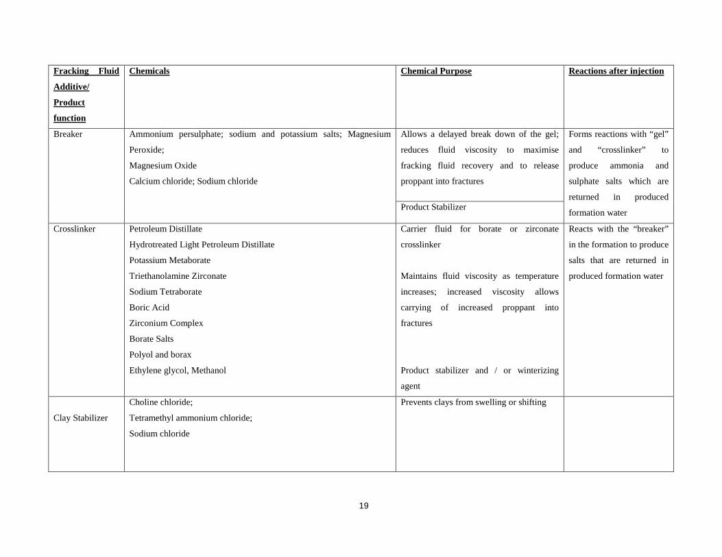
Table 2-1: Breakdown reactions of fracking fluid additives commonly used in water fracturing solutions (Adapted from: Colborn et al., 2011; Earthworks, 2012; GWPC & IOGCC, 2014b; McElreath, Undated)

Fracking Fluid

Additive/

Product

function

Chemicals Chemical Purpose Reactions after injection

Acid Hydrochloric acid Helps dissolve minerals and initiate cracks

in the rock

Reacts with minerals to

produce salts, water and

CO2

Corrosion

Inhibitor

Alcohols ( Isopropanol,

Methanol);

Organic acid and polymer, sodium salt; Formic Acid

Acetaldehyde

N,N-dimethyl formamide, and oxygen scavengers, such as ammonium

bisulphite.

Product stabilizer and / or winterizing

agent

Bonds with pipe surfaces,

broken down by micro-

organisms or returned in

produced formation water Prevents the corrosion of the pipe and all

other steel equipment

Iron Control Sodium compound; citric acid or hydrochloric acid;

Acetic Acid

Thioglycolic Acid

Sodium Erythorbate

Prevents precipitation of metal oxides Reacts with minerals,

producing salts, water and

CO2

Anti-Bacterial

Agent/ Biocide

Gluteraldehyde and an alcohol; sodium salt, sodium hydroxide, and a

bromide salt to form a bromine-based solution;

Quaternary Ammonium chloride;

Tetrakis Hydroxymethyl-Phosphonium Sulphate

Eliminates bacteria growth in the water

that produces corrosive by-products and

gasses and reduce the ability of fluid to

carry proppant into fractures

Broken down by micro-

organisms/ small amount

returned in formation

produced water

17

Fracking Fluid

Additive/

Product

function


Scale Inhibitor Alcohols, organic acid and polymer, sodium salt, ethylene glycol, and

amide:

Copolymer of Acrylamide and Sodium Acrylate

Sodium Polycarboxylate

Phosphonic Acid Salt

Prevents scale deposits in the pipe Attaches to the formation;

though majority returns

with produced formation

water

Friction Reducer

Polyacrylamide

Polymer and hydrocarbon;

Potassium chloride or polyacrylamide-based compounds

Petroleum Distillate

Hydrotreated Light Petroleum Distillate

Ethylene Glycol, Methanol

“Slicks” the water to minimize friction

Carrier fluid for polyacrylamide friction

reducer


agent.

Resides in formation;

broken down by micro-

organisms/ small amount

returned in formation

produced water

18

Fracking Fluid

Additive/

Product

function


Surfactant Lauryl Sulphate Used to increase the viscosity of the

fracture fluid

Returned with produced

formation water or

produced natural gas

Ethanol

Methanol

Isopropyl Alcohol

2-Butoxyethanol

Alcohol, glycol and hydrocarbon


agent.

Naphthalene Carrier fluid for the active surfactant

ingredients

Gelling Agent Guar gum, Polysaccharide Blend

Petroleum Distillate


hydrocarbon, and polymer

Ethylene glycol, Methanol

Thickens the water in order to suspend the

sand

Carrier fluid for guar gum in liquid gels


agent.

Broken down by breaker

and is returned with

produced formation water

19

Fracking Fluid

Additive/

Product

function


Breaker

Ammonium persulphate; sodium and potassium salts; Magnesium

Peroxide;

Magnesium Oxide

Calcium chloride; Sodium chloride

Allows a delayed break down of the gel;

reduces fluid viscosity to maximise

fracking fluid recovery and to release

proppant into fractures

Forms reactions with “gel”

and “crosslinker” to

produce ammonia and

sulphate salts which are

returned in produced

formation water Product Stabilizer

Crosslinker Petroleum Distillate


Potassium Metaborate

Triethanolamine Zirconate

Sodium Tetraborate

Boric Acid

Zirconium Complex

Borate Salts

Polyol and borax

Ethylene glycol, Methanol

Carrier fluid for borate or zirconate

crosslinker

Maintains fluid viscosity as temperature

increases; increased viscosity allows

carrying of increased proppant into

fractures


agent

Reacts with the “breaker”

in the formation to produce

salts that are returned in

produced formation water

Clay Stabilizer

Choline chloride;

Tetramethyl ammonium chloride;

Sodium chloride

Prevents clays from swelling or shifting

20

Fracking Fluid

Additive/

Product

function


Non-Emulsifier Lauryl Sulphate

Isopropanol

Ethylene Glycol

Used to prevent the formation of

emulsions in the fracture fluid


agent.

pH Adjusting

Agent

Sodium Hydroxide

Potassium Hydroxide

Acetic Acid

Sodium Carbonate

Potassium Carbonate

Adjusts the pH of fluid to maintain the

effectiveness of other components, such as

crosslinkers

21

It may come across that the chemicals used in the process would have minor effects as they are

returned with produced formation water, and could thus be captured again. The question one

should be asking is- where does this formation water travel to and is it realistically possible to

recapture all produced formation water?

In the study conducted by McElreath (undated), the conclusions were made that an increase in

temperatures and pressure, as well as the chemical interactions of substances in the fluid itself,

causes the form of most components to change. It essentially affects the fate and transport of

fracking fluid components. The TDS value is prognostic of the concentration of the other species

present in the fluid. Another conclusion to note is that it is well recognised that radionuclides are

present in shale formation water (McElreath, Undated).

2.1.3 Groundwater pollution due to NAPLs

Some groundwater pollutants are also known as NAPLs (non-aqueous phase liquids). These

components include solvents, toxic organic chemicals and petroleum hydrocarbons such as

methane. They have solubility and concentration limitations in aqueous solutions, but these

limitations can already exceed the acceptable concentration that is predetermined for potable

water. NAPLs can therefore usually be in excess of that which is tolerable for good quality

water. Furthermore, inorganic polymers, a range of natural ligands can act as intermediates that

transport NAPLs towards aquifers (Berkowitz et al., 2008).

Dense non-aqueous phase liquids are referred to as DNAPLs. These liquids are denser than water

and can sink deep into the saturated subsurface, while LNAPLs are the light non-aqueous phase

liquids, due to its density which is lower than that of water and will therefore, float on the water

table (Eby, 2004). These compounds (LNAPL’s) may thus migrate upwards by way of density,

with rising water levels and potential geological pathways to shallower aquifers, when it is

released deep in the subsurface by the shale fractures or when present in the fracking fluid.

Common LNAPL’s include benzene, toluene and xylene (Lesage & Jackson, 1992; USGS,

2014a).

The presence of the subsurface gaseous phase and biologically produced gas below the water

table, results in the occurrence of gases in groundwater, where NAPLs may become captured due

to its retention capacity (Berkowitz et al., 2008).

22

2.1.4 Transportation of hydrocarbons and uranium in the subsurface

The composition of groundwater is controlled by chemical and biochemical interactions between

the groundwater and the geological formations through which it flows. The composition is also

influenced by the chemistry of water that flows into the system (Berkowitz et al., 2008).

As mentioned in Section 2.1.1 the fracking process entails the pumping of the fracking fluid into

the subsurface in order to promote the fracturing of shale formations. This fluid consists of

various substances which have a great influence on the chemistry of the water that is used in the

fluid. These chemicals therefore, also influence the water chemistry of the groundwater.

Due to its partial insolubility, NAPLs remain in a distinct liquid phase when transported to the

subsurface. The density and viscosity of the NAPL predominantly governs the migration thereof.

Volatilization of components in the NAPL influences the rate and pattern of migration as well.

When NAPLs enter the subsurface, the physical properties may be transformed when they are

further distributed. Groundwater quality deteriorates when a pollutant plume of NAPLs enters an

aquifer, for the reason that it will be subject to a continuing, incessant slow redistribution, caused

by groundwater flushing-dissolution processes. This may subsequently lead to extensive

pollution over large aquifer volumes. With time, the geometry, solubility and age of the NAPLs

change (Berkowitz et al., 2008).

Petroleum Hydrocarbons (PHs) represents a group of compounds which are categorized as

complex mixtures of hydrocarbons and are often referred to as LNAPLs when they occur in a

separate phase. When ample amounts of PHs are exposed to the groundwater system, it will

continue to migrate until a physical barrier restricts further movement thereof (Berkowitz et al.,

2008).

Uranium exposure to water resources due to fracking is also raising concerns. A report on the

solubility of uranium from the University of Buffalo in the USA (2011), deals with the possible

mobility and migration of uranium for the duration of the hydraulic fracturing process. Results

indicated that uranium has a physical and chemical connection with hydrocarbons (Fortson et al.,

2011; Steyl et al., 2012). Uranium deposits are abundantly present in formations in the Karoo

region, such as the Beaufort Group of the Karoo Supergroup (Department of Mining, 1976). An

overview of uranium, fracking and associated medical threats is discussed in Appendix B.

23

2.2 The Karoo Supergroup

The Karoo Supergroup underlies the Karoo region in Southern Africa and serves as a component

in the stratigraphic framework of the Kaapvaal Craton. The Karoo Supergroup is associated with

mafic and felsic volcanics and consists mainly of sedimentary rocks. The Karoo Supergroup has

an age of approximately 180 Ma as it was deposited after the Cape Supergroup. The sedimentary

rocks were deposited in the inland Karoo Sea which formed behind the Cape Mountain range

(McCarthy & Rubidge, 2005). The crust of the Cape Supergroup began to sag under a load of

mountain ranges, forming a basin in a northern direction. A whole new cycle of sediment

deposition formed the Karoo Supergroup in this basin. Due to the asymmetry from north to south

in the Karoo Sea, the thickness of this Supergroup is also greater in the south and reaches

thicknesses of 8000 m, against the Cape Mountains and thins out towards the north. The surface

altitudes are the highest in the eastern part of the basin declining towards the west, with heights

above mean sea level ranging between 3650 and 800 m. Karoo basalt and dolerite intrusions,

followed by subsequent intrusions of kimberlite and localised mantle up-welling also occurred

(Woodford & Chevallier, 2001). Dyke events associated with the Karoo Supergroup is under

alia- the Rooi Rand Dyke Swarm, Okavango Dyke Swarm, Olifants River Dyke Swarm and the

Karoo Dolerite Suite. Dykes are mainly dolerite intrusions. Vertebrate remains such as mammal-

like reptiles and dinosaurs as well as fossils of insects and plants, are well represented in the

Karoo Supergroup (Johnson et al., 2006; Lurie, 1979 and McCarthy & Rubidge, 2005).

Table C-1 in Appendix C represents the lithology of the Karoo Supergroup, describing each

Group within the Basin. Each Group corresponds to a certain environment of deposition. Fluid

migration and progressive diagenesis also played a role in the development of the main Karoo

Basin (Woodford & Chevallier, 2001).

24

For the precedent 250 million years, the Karoo has been a vast inland basin. Dwyka tillites which

is widely-distributed in the area reveals evidence that the area was glaciated at one stage.

Afterwards, great inland deltas, seas, lakes or swamps were present consecutively. Throughout

these stages substantial deposits of coal formed. Volcanic activities also occurred immensely

(Svensen et al., 2006). Dolerite intrusions outcrops over almost two thirds of South Africa and

are mostly associated with the Karoo Supergroup (Chevallier &Woodford, 1999).

2.3 Characteristics of formations in the Study Area

Gravity is the dominant driving force for the movement of groundwater and causes the process

of groundwater recharge. The mineral compositions of the layers through which the water move

influence the groundwater chemistry and quality (Appelo & Postma, 2005; Grotzinger et al.,

2007).

The rocks present in the Victoria West subsurface are mainly, sandstone, mudstone, dolerite and

shale with varying thicknesses. Some of these formations contain other interbedded minerals in

the layers. In the immediate subsurface, sandstone is mainly found, followed by mudstone layers,

intruded by dolerites. Deeper in the subsurface, shales are present, and are the source from which

methane will be extracted. Kimberlite intrusions are also present in some areas (Council for

Geoscience, 2013). Dolerite and kimberlite intrusions may contribute to subsurface flow as they

are associated with faults which may serve as pathways, for groundwater movement (Steyl et al.,

2012).

The Karoo Basin is displayed in Figure 2-6. Table 2-2 displays the lithology and associated

characteristics present in the Karoo Supergroup, describing each Group within the Basin. Each

Group corresponds to a certain environment of deposition. Fluid migration and progressive

diagenesis also played a role in the development of the main Karoo Basin (Woodford &

Chevallier, 2001).

http://sajg.geoscienceworld.org/search?author1=L.+Chevallier&sortspec=date&submit=Submit

http://sajg.geoscienceworld.org/search?author1=A.+Woodford&sortspec=date&submit=Submit

25

Figure 2-6: Geology of the main Karoo Basin (Constructed from shape files obtained from Council for Geoscience, 2014; StatSilk, 2014)

26

Table 2-2: Lithology and associated characteristics present in the Karoo Supergroup applicable to this study (Coetzee, 2008)

Lithology Rock Type Mineral assemblage

Characteristics Group/ Formation location

Sandstone Clastic sedimentary rock

Quartz Feldspars (Na- and K-rich) Mica Carbonates Clay minerals (Silicates) Can also be distinguished as a carbonate rich rock

Deltaic sandstone facies of the Ecca group: serve as good water sources, although it can have low permeabilities. Middle Ecca sandstones: moderate primary porosity and permeability. Fine-grained sandstone of the Beaufort group: low primary permeabilities. Coarse-grained sandstones at base of Molteno formation: good aquifers. All coarse grained layers: higher permeabilities than that of fine-grained units. The Clarens formation sandstones: well-sorted, medium- to fine-grained units, with a high average porosity of 8.5%. However- it has a low permeability. Sandstones south of latitude 29 S: very low primary porosity and permeability (Woodford & Chevallier, 2001).

Ecca Group Beaufort Group Stormberg Group: Molteno, Elliot and Clarens Formations

Mudstone Fine-grained clastic sedimentary rock

Quartz Mica Clay minerals (Silicates: kaolinite, montmorillonite and illite) Iron Hydroxides and Iron Oxides

Mainly consist of silt- and clay-sediments May contain carbonates. Eroded easily, but have low permeability and porosity when compacted and intact. Poor aquifers. Beaufort group mudstones: low permeabilities. Elliot formation: largely composed of red mudstones, making it a low transmissive formation due to relative impermeability. Elliot formation mudstones: very porous, allowing them to leak water into other, more permeable formations, such as underlying Molteno formation (Grotzinger et al., 2007; McCarthy & Rubidge, 2005 and Woodford & Chevallier, 2002).

Beaufort Group Stormberg Group: Molteno and Elliot Formations

http://en.wikipedia.org/wiki/Kaolinite

http://en.wikipedia.org/wiki/Montmorillonite

http://en.wikipedia.org/wiki/Illite

27

Dolerite Phaneritic intrusive igneous rock

Quartz Amphibole Plagioclase Pyroxene Olivine

Flood basalts are acknowledged to have been originated from large mantle plumes. The upward flow of peculiarly hot material from the base of the lithosphere, were caused by these plumes. It furthermore generated an exceptionally great amount of hypabyssal (rocks that occur in the form of dykes) dolerite dykes and sills in the basin, which outcrops on the surface of the Karoo Supergroup. These structures are the most common intrusion present in the Karoo basin. The geomorphology and drainage system of the Karoo Basin are mainly controlled by these intrusions as they display circular patterns, known as ring structures. Dolerites are very low permeable, dense, confined rocks. (Steyl et al., 2012; Woodford & Chevallier, 2001).

Intrusions

Shale Fine-grained clastic sedimentary rock

Quartz Mica Clay minerals (Silicates: kaolinite, montmorillonite and illite) Iron Hydroxides and Iron Oxides

Shale is a highly compacted, non-porous, dense rock through which virtually no water moves. Primarily composed of clay minerals and organic material Dwyka group shales: Hydraulic conductivities ranging between 10-16 and 10-17 m/day, therefore aquitards. Ecca group shales: thicknesses ranging between 1500 m in the south, to 600 m in the north. Porosity of 0.10% north of latitude 28˚ S, and less than 0.02% south of latitude 28˚ S. General average porosity for shales of the Karoo: ranges between 2 and 10%, north of latitude 31 S and less than 2% south of latitude 31 S. Beaufort group shales: low permeabilities (Woodford & Chevallier, 2002).

Dwyka Group Ecca Group

Kimberlite Porforitic Intrusive igneous rock

Olivine Phlogopite Ilmenite Perovskite Carbonates Enstatite Cr-Diopside Chlorite

Alkaline ultramafic rock which occurs in pipe structures and therefore may serve as pathways for water and fluids (McCarthy & Rubidge, 2005). When in contact with water, sodium and magnesium rich fragments dissolve and the total dissolved solids (TDS) of the water increases (Huizenga, 2011a; Pretorius, 2012). Low permeability

Intrusions




28

2.4 Shale

Shale is a clastic sedimentary rock which is primarily classified in relation to mineral grain sizes.

Clastic rocks are also referred to as detrital or allocthonous which describes those rocks, formed

by weathering of pre-existing rocks, erosion, transport and deposition. Shale is generally formed

due to compaction processes. Shale refers to a mud rock which is the finest grained clastic

sedimentary rocks, comprising grain sizes with diameters of less than a sixteenth of a millimetre

(Cairncross, 2004). Minerals present in shale, are typically quartz, mica, iron oxides and –

hydroxides and clay minerals such as kaolinite, montmorillonite and illite (King, 2013). Shale

can be layered, also known as laminated as the rock is made up of many thin layers. Shale is also

fissile, in other words, the rock can readily split into thin pieces along the laminations (Coetzee,

2008). Due to the fissile nature of shale, the fracking process is facilitated as fracturing of the

rock formation will be unprompted.

Black organic shale is the host for the most noteworthy oil and natural gas deposits in the world

(King, 2013). When carbonaceous material is more than 5% present in shale, it indicates a

reducing environment such as stagnant water columns. Such an anoxic environment has black

shale as result due to anaerobic decay of organic matter that was deposited with the mud in

marine or lacustrine basins from which the shale formed (Steyl et al., 2012). In the forming

process of shale, this mud undergone a burial and heating period within the earth and during this

process a quantity of the organic material was mutated into oil and natural gas (King, 2013).

Therefore hydrocarbons can also form in the subsurface due to diagenetic processes that is

caused by increased pressures and temperature during the burial of the material (Tourtelot,

1979).

Black shale contains reduced free carbon along with ferrous iron and sulphur as sulphide

minerals are deposited due to reducing conditions in the shallow subsurface. With increased

depth, fermentation processes occur and produces biogenic methane. At greater depths

decarboxylation reactions and thermal maturation that produces additional hydrocarbons take

place (Tourtelot, 1979).

These shales are dark in colour due to pyrite and amorphous iron sulphide as well as unoxidized

carbon which is present in large amounts. Some black shales may contain heavy metals in large




http://en.wikipedia.org/wiki/Redox

http://en.wikipedia.org/wiki/Pyrite

http://en.wikipedia.org/wiki/Oxidation

http://en.wikipedia.org/wiki/Carbon

29

numbers. Some of the known heavy metals found in this rock include molybdenum, uranium,

vanadium, and zinc (Lüning, Undated).

2.5 Natural Gas

Natural gas is a resource which usage is fast becoming popular for energy production, due to the

decline of other energy sources. The estimation of obtainable natural gas is increasing with time

as this technique is being implemented by more companies worldwide and therefore the

availability of natural gas is explored intensively. Due to increased exploration, coal seams and

very deep lying shale formations have been identified in prospecting areas (Grotzinger et al.,

2007).

Petroleum refers to any fluid which is rich in hydrocarbons. This hydrocarbon-rich fluid

originates from kerogen, a polymeric organic material which is present in sedimentary rocks in

the form of finely disseminated organic marcelas. Kerogen is altered to petroleum through

reactions caused by increased temperature and pressure, in the diagenetic environment, which

refers to the environment in which processes are present, at pressures and temperatures that lie

between the weathering and metamorphic environment. These reactions produce carbon dioxide

(CO2) and methane (CH4). Methane is a dry gas which signifies the final stage of hydrocarbon

thermal maturation (Steyl et al., 2012). Methane is part of the alkane group, and also a

hydrocarbon due to its chemical composition and arrangement. The fine-grained components of

shales absorb gaseous hydrocarbons, which refers to methane to pentane. These hydrocarbons

can be desorbed by low-temperature acid hydrolysis (Rowsell & De Swardt, 1976).

The process for hydrocarbon formation in source rocks is illustrated in Figure 2-7 that gives an

indication of the temperatures and depth at which natural gas forms. Figure 2-7 supports the

importance of the thermal history of a basin as it reflects its oil-producing capability (Eby, 2004).

The evolution and maturation of kerogen is described by the processes of (1) diagenesis, (2)

catagenesis and (3) metagenesis. Diagenesis describes the process in which kerogen undergoes

the first stage of degradation, where oxygen decreases as carbon increases with depth. In this

stage the kerogen is still immature and only traces of hydrocarbons which were produced from

the host rock, are present. The second stage of kerogen degradation is explained by the process

of catagenesis. This is where a rapid decline in hydrogen content is observed as a result of

30

hydrocarbon generation with depth. Catagenesis is the stage which not only presents the oil

window, it also points to the initiation of cracking that produces “wet gas” with increasing

methane content. The final stage of kerogen degradation is the process of metagenesis which

entails the gradual elimination of the remaining kerogen which consists out of two or more

carbons. Metagenesis takes place in the “dry gas” zone (Flores, 2014). Oil is formed at a burial

depth between 2 and 4 km, wet gas is produced between 4 and 5 km, and at a depth of 5 to 6 km,

dry gas is produced (Steyl et al., 2012).

Figure 2-7: Illustration of petroleum production from a reservoir rock assuming an average geothermal gradient (Adapted from Eby, 2004 and Steyl et al., 2012)

Natural gas mostly refers to methane (CH4) (Eby, 2004). During combustion it reacts with

atmospheric oxygen. This reaction releases energy in the form of heat and produces carbon

dioxide and water. Thus, through this reaction, fewer pollutants are released compared to the

31

products of combustion reactions of coal and oil (Eby, 2004; Steyl et al., 2012). Methane

releases 30% less carbon dioxide than oil and 40% less carbon dioxide than coal per unit of

energy; therefore the resource is more efficient and explains the motivation for increased

demands (Grotzinger et al., 2007). This is exemplified in Equation 2-1.

32

Equation 2-1: Example of carbon dioxide produced for the constant amount of energy of 106 KJ (Huizenga, 2011b)

33

In the examples above it is indicative that methane produces the least amount of carbon dioxide

for the same amount of energy (Huizenga, 2011b). Therefore the process of fracking will not

only solve the crisis concerned with depleting energy resources, it will also improve the negative

factors that are involved in the energy producing processes.

2.6 Geological Structures

2.6.1 Dykes and sills

Figure 2-8 shows the geological structures of dolerite in the Victoria West area, which will be

the study area for this investigation. Major dykes and faults might have a significant influence on

the movement of groundwater and hydraulic fluids (Steyl et al., 2012). In the area of the main

Karoo Basin, faults with strike lengths of more than 5 km, commonly intersect the Karoo strata.

This occurrence is confirmed by maps of this region, which can be obtained by the Council for

Geoscience, South Africa (Hill, 1993).

34

Figure 2-8: Map of Victoria West Dolerite Sill and Ring Complex (Adapted from: Chevallier et al., 2001)


35

These structures may possibly serve as a key component in deep groundwater circulation and

migration of hydraulic fluid as they may serve as pathways along which migration can occur


2.6.2 Sill and Ring-Complexes

Sill and ring-like structures are formed by early Jurassic dolerite intrusions. They commonly

exhibit a saucer-shape, comprising an inner sill at the bottom, an acute inclined sheet on the

periphery, and on the rim an outer sill is present (refer to Figure 2-9) (Chevallier & Woodford,

1999). Studies of the Karoo confirm that the general saucer-shape of sill and ring-complexes

exhibits a flat-lying inner sill in depressions and an elevated outer sill in higher grounds

(Chevallier et al., 2001). Relatively vertical dykes can branch onto sill and ring complexes or cut

through them. The lithology of the western Karoo contains dykes which feeds into the inclined

sheet, controlling the shape of the ring. Some dykes (vertical) link ring structures as they branch

out of one ring into another. Dolerite sill and ring-complexes, although referred to as circular,

may have irregular outlines and consequently may also intersect one another. A hydro-morpho-

tectonic model of a typical dolerite ring structure is illustrated in Figure 2-9, where morpho-

tectonics refer to the study of superficial evidences of tectonic activity and this mainly influences

the drainage parameter and the interaction with geological structures that controls the direction

of flow. The Victoria West region (north of latitude 32° 45’) comprises an intense complexity

and interconnectivity of intrusions (Chevallier et al., 2001; Council for Geoscience, 1997) which

may serve as groundwater migration pathways. Figure 2-10 indicates the dolerite geology

surrounding Victoria West and also indicates where Victoria West is situated.

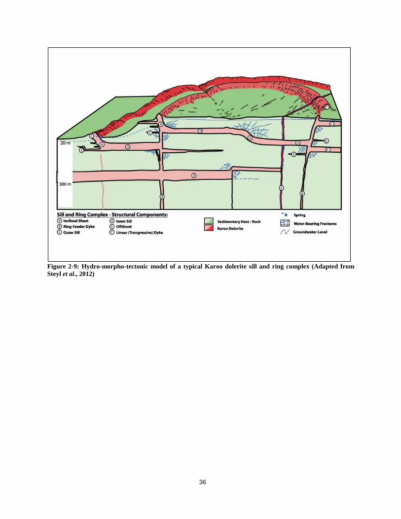
36

Figure 2-9: Hydro-morpho-tectonic model of a typical Karoo dolerite sill and ring complex (Adapted from Steyl et al., 2012)

37

Figure 2-10: Map of dolerite geology surrounding Victoria West (Constructed from shape files obtained from Council for Geoscience, 2014; StatSilk, 2014)

All of the faults, north of latitude 32° 45’ (refer to Figure 2-10) are mainly associated with

dolerite. In this area, sills caused sedimentary rocks to be uplifted and the displacement is

directly proportional to the thickness of the sill, although there are indications that the dolerite

dykes may possibly be associated with pre-existed faults, which offered channels for dolerite

intrusions. All fractures along the dykes (vertical) and sills (horizontal) may act as passages

which may promote groundwater migration (Hill, 1993; Steyl et al., 2012). These numerous

dykes and sills occur and therefore concerns are raised regarding groundwater systems that might

carry fracturing fluids to natural aquifers in this area (Steyl et al., 2012).

Intrusive dolerites are present in an area which covers more than 390 000 km² of the main Karoo

Basin, which is underlain by the Ecca Group (Svensen et al., 2006). Dolerite intrudes as a

network of interconnected dykes and sills (Chevallier et al., 2001). The network of dolerites is

dense at regional scale. These intrusions are not present in the southernmost part of the basin,


38

which is south of latitude 32°45’S. In regions where dolerite networks are less dense, the

connectivity between intrusions is remarkably low due to 1km spacing between them.

Intrusion of dolerites through neighboring shale formations could have possibly caused a thermal

increase which lead to pyrolysis (thermochemical decomposition of organic material) and

consequently, the decomposition and reduction of organic carbon in the shales (Rowsell & De

Swardt, 1976; Svensen et al., 2006).

Therefore, where dolerites are concentrated through shale formations, the organic carbon and

thus the natural gas content is lower than in areas that contain less dolerite intrusions. These

desolated areas are most probably located between adjacent dolerite sill and ring (oblique) like

structures (Steyl et al., 2012).

However, a relationship between the lithology and dolerite distribution are considered as there

exist an abrupt decline in intrusion density between the lower Ecca and upper Ecca boundary,

with a higher density in the upper region (Woodford & Chevallier, 2002). This abrupt difference

in intrusion density can be noticed where sandstone units begin to occur in the Karoo Basin

(Woodford & Chevallier, 2002). Although dykes can be observed in the lower Ecca and Dwyka

formations, the majority is focused and confined to the Upper Ecca and Beaufort sandstones,

suggesting that the dolerite could have propogated laterally instead of vertically (Chevallier et

al., 2001).

Flat lying dolerite sills are found in the lower Ecca and Dwyka formations. The host rock of

these sills is homogeneous shales with fine lamination and high-grade anisotropy. Large dolerite

basin structures are found in the upper Ecca Group, Beaufort Group and to an extent, certain

overlying formations. The explanation of the presence of basin structures in the upper groups is

based on the principle that was developed by Van Zijl (2006) that proposes that intrusion of

magma always follow easiest flow paths. The interconnection of lenticular sandstones

interpolated with shales and mudstones in the upper formations thus provide a matrix that

provides less resistance for magma intrusion than the homogeneous shales with fine lamination

in the lower Ecca and Dwyka formations (Van Zijl, 2006).




39

The sills and inclined sheets encompass thicknesses which range from a few meters to 200 m.

Dykes usually exhibit dips which vary between vertical to 70°. Dykes generally ranges between

2 and 15 m in width and 5 to 30 km in length, but can reach distances up to 80 km (Duncan &

Marsh, 2006). Horizontal drilling might furthermore intercept a dolerite dyke as the drilling can

take place over a number of kilometres. The dolerite dyke, comprising an east-west strike, which

lies north of Victoria West reaches thicknesses of 65 m in some places (Steyl et al., 2012).

2.6.3 Dolerite sill/ring complexes and groundwater

Most of the second-order geomorphological features and drainage systems of the Main Karoo

basin are controlled by dolerite rings and sills (Chevallier et al., 2001). When taking strikes and

yield into consideration, planar fractures which are connected with lithological contacts or

dolerite sills, can be accepted as significant groundwater targets in the Karoo. This is confirmed

in various Water Research Commission projects (Botha et al., 1998; Botha & Cloot, 2004;

Chevallier et al., 2001; Chevallier et al., 2004a; Chevallier et al., 2004b; Chevallier &Woodford,

1999; Woodford & Chevallier, 2002), wherein plentiful groundwater strikes were intercepted at

depths reaching 300 m (Steyl et al., 2012).

Therefore, the existence of water supply boreholes in these regions which need to continue with

the providing of usable quality water cannot be neglected. Furthermore, these boreholes can

serve as high conductivity pathways for water and fluid migration, however, the presence of

water strikes as well as their properties at depths below 300 m in the Karoo stratigraphy, are not

certain and should still be determined (Steyl et al., 2012).

Nearly all water strikes are present in sediments clear of the dykes and appear to be connected to

horizontal or transgressive oblique fractures, consequential of cooling joints or horizontal offsets

along the dyke, that intercept the dyke and extends into the surrounding formations. Thermal

joints are created in the intrusion, perpendicular to the cooling surface as well as in the

immediate sediments. The thicknesses of intrusions establish the distance, ranging between one

to a number of meters, by which the adjoining rocks are affected by thermal jointing. In the

weathered zone, most water strikes are associated with the contact dyke-sediment, while below

the depth of 70 m less water strikes are present alongside transgressive fractures (Steyl et al.,

2012). The probability for water migration due to additional fractures created in deeper


40

formations by the fracking process, which could possibly intersect with existing faults of

fractures, will be considered in this study.

Sub-horizontal fractures may be the most important mechanism controlling flow dynamics at

depth and in the region of dykes as they are not interconnected, but are supplied with water

through the surrounding host rock matrix. Therefore the vertical groundwater circulation appears

to be influenced at a minor extent by dolerite dykes at depth. Different case studies also reveal

that low hydraulic conductivity values restrict major flow within the dykes. Hydraulic fracturing

due to horizontal drilling is limited as these fractured aquifers at depth are also very confined.

This also minimizes the probability for series of individual fractures to be affected or polluted,

even more so if hydraulic fracturing takes place at depths greater than 1500 metres (Steyl et al.,

2012).

However, natural thermal springs also occur in the main Karoo Basin, and have temperatures

ranging between 26 and 41°C. More or less 16 of these springs are present to the south of

latitude 28 S. These waters originate at depths ranging between 450 and 1150 m. The high

temperatures cause differences in fluid densities and subsequently cause water to travel upward

at faster rates, therefore natural connections between deep groundwater and the surface exist,

although dolerite dykes and sills may restrict these migrations (Steyl et al., 2012).

2.6.4 Kimberlite fissures

Environments, in which Kimberlites are found, ought to be taken into account in any exploration

drilling activities due to the presence of fracturing systems they could occur in. Kimberlite

fissures can also possibly be intersected in the horizontal drilling process. These fissures extend

from great depths as they originated at the base of the craton, located 30 to 40 km below surface.

Parallel fissures and related joints or fractures occur in kimberlite fracture swarms, which are

divided into smaller sub-swarms wherein the fissures lie close together with 10 to 50 m spacing

and comprising thickness of 0.5 to 4 m. Fissures comprising the latter widths are usually

associated with the upwarpment of surrounding Karoo layers. Parallel regional jointing and the

fissures usually accompany one another. The presence of sub-swarms indicates a vertical

hierarchy deep in the fracturing system, such as fissures, dykes, parental dykes and larger bodies.

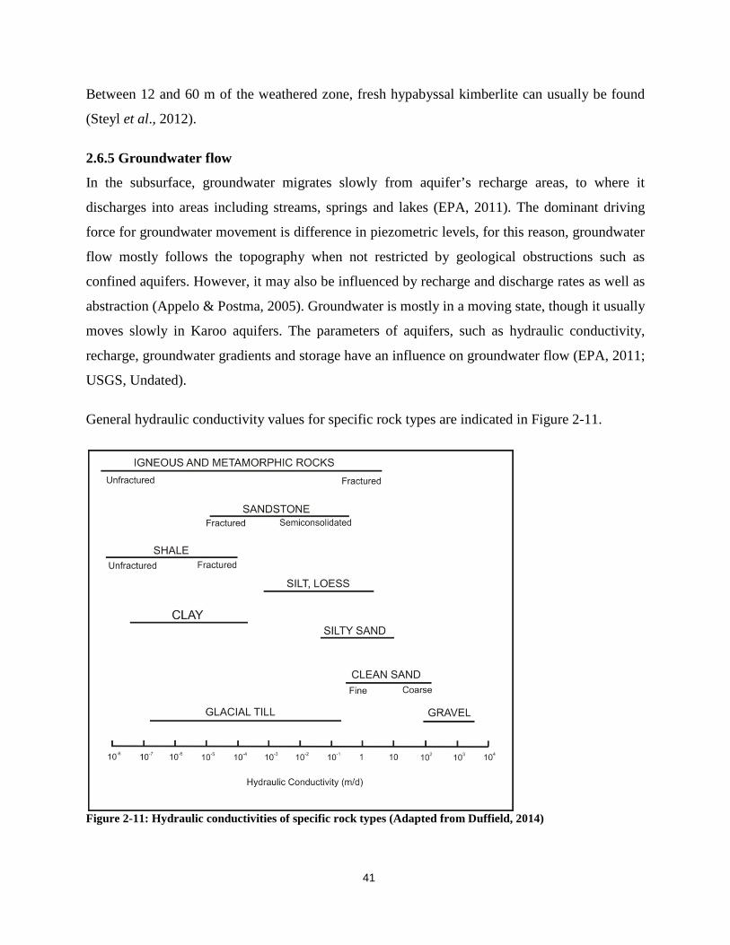
41

Between 12 and 60 m of the weathered zone, fresh hypabyssal kimberlite can usually be found


2.6.5 Groundwater flow

In the subsurface, groundwater migrates slowly from aquifer’s recharge areas, to where it

discharges into areas including streams, springs and lakes (EPA, 2011). The dominant driving

force for groundwater movement is difference in piezometric levels, for this reason, groundwater

flow mostly follows the topography when not restricted by geological obstructions such as

confined aquifers. However, it may also be influenced by recharge and discharge rates as well as

abstraction (Appelo & Postma, 2005). Groundwater is mostly in a moving state, though it usually

moves slowly in Karoo aquifers. The parameters of aquifers, such as hydraulic conductivity,

recharge, groundwater gradients and storage have an influence on groundwater flow (EPA, 2011;

USGS, Undated).

General hydraulic conductivity values for specific rock types are indicated in Figure 2-11.

Figure 2-11: Hydraulic conductivities of specific rock types (Adapted from Duffield, 2014)

42

2.6.6 Groundwater chemistry

Groundwater systems and surface water bodies interact as water is interchanged between these

two hydrologic system components. The degradation of one affects the quality of the other

(Winter, 2000).

The chemical processes that occur in water, are influenced by various environmental factors. The

chemistry of South African water systems are, primarily controlled by the chemical weathering

of rocks. The total dissolved ions present in natural waters, is derived from underlying or

surrounding rocks, or may have been derived from rain (Appelo & Postma, 2005; Bucas, 2006

and Huizenga, 2011a). More information regarding weathering processes which primarily

control water chemistry, as well as rock weathering of rocks relevant in this study, are found in

Appendix D.

2.6.6.1 Climate

The amount and rate of rainfall, runoff and evaporation, influence and controls water availability

and the composition of water and solutes (Hem, 1989). The chemical composition may vary, as

the volume of flow of run-off can fluctuate and influence the dilution factor. The chemical

composition of water is also influenced by climatic patterns which produce characteristic plants

and soil types. Some ions are influenced by climate, to a greater extent than other components.

High temperatures increase the solubility and dissolution rate of minerals. Hot and humid climate

regions usually contribute to the highest weathering rates of rocks. The weathering rates of rocks

depend on runoff, and for a given runoff value, chemical weathering increases with temperature

(Bucas, 2006; Hem, 1989).

2.7 Karoo Aquifers

2.7.1 Properties and parameters

Due to the fact that the Karoo covers a great area of the surface of South Africa (Lurie, 1979),

the importance of the groundwater resource is even more crucial as there are limited resources in

this section of South Africa. The Karoo aquifers are also secondary aquifers, which refers to rock

formations that owe its water-bearing capacity to fracturing. The groundwater is mainly stored in

the sedimentary rocks. Therefore the fractures are not the main storage units for water in the

43

Karoo, although the fractures assist in the movement of groundwater and act as conduits through

which groundwater and pollution can move (Woodford & Chevallier, 2002).

The Karoo Supergroup mainly consists of sandstone, mudstone, shale and siltstone formations.

These rocks exhibit a permeability ranging from moderate (sandstone) to very low (shale).

Therefore, the majority of boreholes drilled in the Karoo formations have immediate yields of

less than one litre per second. Although the Karoo is known for its dry and arid properties,

encompassing aquifers with a limited yield, sufficient volumes of groundwater are daily pumped

for surrounding towns and from mines, underlain by the Karoo formations (Woodford &

Chevallier, 2001).

Karoo sediments have higher porosities closer to the surface of the earth, possibly due to

weathering and leaching of the rocks within the first 30 m below surface. Correspondingly,

increasing lithostatic pressures and temperatures causes decreased primary porosity with depth

(Woodford & Chevallier, 2001).

Estimations of regional groundwater flow parameters such as hydraulic conductivity and

storativity values in the Karoo formations are complicated due to the presence of dolerite dykes

and sills which encompass uneven distributions of zones with varying permeability values.

Ephemeral rivers flow in the central and western Karoo Basin, subsequent to heavy rainfalls,

therefore only contributing to the groundwater systems in these periods. There is also very little

run-off in the Karoo area due to a flatter topography in the west. Highest evaporation records

occur in the duration of the hot summer months, leading to additional decreases in the available

water of the area (Woodford & Chevallier, 2001).

2.7.1.1 Aquifer parameters in Victoria West

The groundwater resource potential in the Victoria West region ranges from 10 000 to 15 000

m3/a /km2 (Van Tonder, 2012). The depth to the groundwater level mainly ranges from 5 to 20

mbgl. The Electrical Conductivity (EC) in the area ranges from below 70 to 150 mS/m (Van

Tonder, 2012) and averages at 126.8 mS/m for the boreholes in the D61E catchment (National

Groundwater Archive, 2013). Karoo formations exhibit immediate yields of < 1 L/s (Woodford

& Chevallier, 2001). The transmissivity ranges for different aquifers in the Karoo. The

44

transmissivity ranges from 20 m2/day for sandstone aquifers and 2 to 5 m2/day for shales, which

rather categorizes them as aquicludes. The average transmissivity for the Karoo is estimated at 5

to 15 m2/day. The percentage of rainwater recharging the Karoo aquifers ranges from 1 to 3% of

mean annual precipitation due to a low rainfall climate region with a precipitation of 245 mm to

480 mm annually (Cobbing et al., 2013; South African Weather Service, 2013). Hydraulic

conductivity for sand sediments such as sandstone varies from 10 to 300 m/day, while the

porosity ranges from 0.1 to 0.15. The shales however have lower porosities ranging from 0.05 to

0.1 and decreases with depth (Cobbing et al., 2013). The storativity values are generally

estimated to be in the range of 10-2 to 10-5 for the aquifers of the Karoo Supergroup (Steyl et al.,

2012).

2.8 Hydrogeological Modelling

Groundwater models are used to communicate information on groundwater flow and pathways,

the groundwater system in which flow occurs, as well as the processes which mainly affects the

system and its behaviour. It is also applied in order to understand the impacts certain operations

could have on the system. The specific objectives, type of results that are desired as well as the

available data of a site determines the type of groundwater model that could be used as different

models can be manipulated in order to provide specific required results.

Recharge Models

Recharge estimation methods in that are generally used in Southern Africa are the Chloride mass

balance (CMB), Cumulative Rainfall Departure Method (CRD), Extended Model for Aquifer

Recharge and Moisture Transport through Unsaturated Hardrock (EARTH), Water Table

Fluctuation (WTF), Groundwater modelling (GM) and Saturated Volume Fluctuations (SVF)

methods. These methods are specifically applied to regions with arid and semi-arid climate. All

available data of the different hydrologic zones are linked by these models in order to estimate

the recharge of an area (Xu & Beekman, 2003).

Chloride mass balance (CMB), Cumulative Rainfall Departure (CRD), Groundwater modelling

(GM) and Saturated Volume Fluctuations (SVF) methods are most general methods which are

applied for recharge estimation due to the fact that more data is used and complexity in these

45

methods is higher than that of other methods (Xu & Beekman, 2003). These different methods

were investigated to ultimately select the method most suitable for this study.

Chloride mass balance (CMB)

The time and aerial distribution of groundwater recharge is combined by way of the chloride

mass balance method (Bazuhair & Wood, 1996), which was introduced by Eriksson &

Khunakasem (1969). The integration of time and space makes it an appropriate method to use in

areas where the variation in time and space is substantial (Bazuhair & Wood, 1996). This method

is based on the approach that the input of atmospheric chloride is equal to the chloride flux in the

subsurface, which basically refers to a mass balance (Xu & Beekman, 2003). It is generally

applied to make estimations on long-term groundwater recharge (Fouty, 1989). Recharge can be

estimated with the excluding of surface water run-off by using this method (Kinzelbach et al.,

2002; USGS, 2014b), which makes groundwater recharge estimation very simple. This method is

also one of the cheapest and less complicated methods to determine recharge (Kinzelbach et al.,

2002).

Chloride method where runoff is neglected

D + P ∙ 𝑐Rp = Rech ∙ 𝑐RRech Rech = 𝑐𝑝 𝑃 +𝐷

𝑐𝑅𝑒𝑐 ℎ

Where P = precipitation (mm per time) Rech = recharge (mm per time) D = dry deposition (in mg per m2 and time) cP = chloride concentration in precipitation (mg/l) cRech = chloride concentration in recharging groundwater (mg/l) (Kinzelbach et al., 2002).

Cumulative Rainfall Departure Method (CRD)

The CRD method is a recharge method that has been used with great success in Southern Africa

(Bredenkamp et al., 1995). This method is based on the principle that rainfall events have an

influence on water levels and is thus the cause for fluctuations to occur (Xu & Beekman, 2003).

It is a simple method that indicated that the cumulative rainfall departure curve (CRD) is

http://www.sciencedirect.com/science/article/pii/S0022169496030284




46

proportional to the changes in water levels. The method can however only be applied to closed

spring catchments and all the parameters that influence the water balance have to be identified

and included (Kinzelbach et al., 2002).

Groundwater modelling (GM)

Groundwater model is a term that is interchangeably used for conceptual groundwater model,

numerical groundwater model or analytical groundwater model. Analytical and numerical

models are mathematical models which exemplify groundwater flow systems.

Essentially, groundwater models are the entirety of a range of physically and mathematically

based components, all adding to the overall understanding of groundwater systems and the

effects of any impacts on it (Kinzelbach et al., 2002). By the numerical modelling of

groundwater flow and the calibration of water levels, recharge can also be determined (Xu &

Beekman, 2003).

Saturated Volume Fluctuations method (SVF)

This method is a time related water balance which is based on the average water levels in

monitoring boreholes and is usually applied when recharge in saturated zones are determined.

Data quality and quantity is a major factor when using this method as a water balance is subject

to the data provided. Limitations of this method include: the complete aquifer must be

represented by measured water levels and inflow and outflow boundaries must be known (Xu &

Beekman, 2003).

Conceptual Models

A conceptual model describes groundwater flow and transport in an area by means of the

available site-specific data or factors that can have any change in hydrogeological processes as a

result. It essentially gives an idea of how a groundwater system should work considering the

given/available information of the system and site by representing the physical hydrogeological

system and its hydraulic behaviour. “An interpretation or working description of the

characteristics and dynamics of the physical system” reflects the definition of the ASTM for a

conceptual model (ASTM D5447-04, 2010). A conceptual model of the study area is indicated in

Section 4.1 in order to give a simple representation of the concept on which the numerical model

was constructed.

47

Mathematical Models

A mathematical model describes the flow in a groundwater system mathematically. The ASTM

defines a mathematical model as the “The mathematical equations expressing the physical

system and including simplifying assumptions. The representation of a physical system by

mathematical expressions from which the behaviour of the system can be deduced with known

accuracy” (ASTM D5447-04, 2010).

Mathematical models include analytical or numerical models; 1D, 2D or 3D models;

groundwater flow models, groundwater flow & transport models; steady-state or transient

models; equivalent porous media or discrete fracture models, etc. Analytical and numerical

models are briefly defined below:

Analytical Models

Analytical models use exact solutions (e.g. Darcy Law, Theis solution, advection-dispersion

equation) of typical flow and transport equations which describes groundwater flow and

contaminant transport respectively to not only define simple systems but also to elucidate broad,

comprehensive effects of different parameter assumptions. Analytical models can be anything

such as simple formulations, databases, worksheets or sequences of calculations that are

enveloped together to form a part of software.

Numerical Models

Complex systems are usually epitomised by numerical models. A numerical model can be

defined as computer model that makes use of finite difference, finite element or other numerical

methods, and produces an estimated solution of the principal groundwater flow and/or

contaminant transport equations. These models can accommodate multiple modelling objectives

which can be solved simultaneously. According to the ASTM a numerical model is “the

application of a mathematical model to represent a site-specific groundwater flow system”

(ASTM D5447-04, 2010). In these models parameter values such as hydraulic conductivity,

porosity, aquifer thickness, initial contaminant concentration, etc. are assigned to each model

grid cell within the model in order to distribute space and time into discrete intervals and build a

model that can represent reality as close as possible.

48

Numerical modelling is a helpful method, used to visualize and predict the behaviour of physical

systems when subjected to certain conditions. This is the model type used in this study. Models

used in the geohydrological sense, usually simulates the flow of groundwater, solute transport,

and reactive solute transport in the subsurface. All available software is very useful if the correct

software that could adequately model the acquired specifications is selected. An adequate

modelling software package for a specific scenario and requirements should therefore be utilized

to ultimately obtain the best and most accurate results. For this reason, several software packages

should be considered in order to make an informed decision as to which software will be used to

model and simulate the relevant factors for the study.

In several studies conducted on the impact of fracking and contaminant transport on groundwater

resources (Das, 2002; Myers, 2012; Tenbus & Fleck, 2001 and Yang et al., 2012), interpretative

MODFLOW- 2000 (Harbaugh et al., 2000) computations and associated programmes therein,

such as SEAWAT, MT3DMS and MODPATH, were used for several potential scenarios of

contaminant transport. Different scenarios have been modelled with these programmes including

the natural upward advective flow of water from deep lying shale formations to the surface, with

and without interconnecting faults and fractures; the simulation of expected flow rates due to

changes in the shale geohydrology imposed by the fracking; and the simulation of the injection

of 13 to 17 million liters of fracking fluid into fractured shale from a borehole with a fault

present and also without a fault, over a specific time period (Myers, 2012). However, this

modelling software does not incorporate all of the structural complexities of the geology and

does model multiphase flow and transport. It cannot model faults, fractures and other structural

geological features with specific angles and conductivities, as it only models porous flow for

layered formations. This could cause miscalculations of the travel times for flow and transport of

contaminants as fractures and faults are not layers, but apertures (Myers, 2012).

Along with MODFLOW, FEFLOW is also an accepted groundwater model in the industry and

significant for simulating fluid flow and transport of dissolved components in the subsurface, this

software also incorporates and simulates fractures and fracturing.

Other software packages such as BIOSCREEN, BIOCHLOR, FOOTPRINT, and REMChlor are

Domenico-based models which are approximate solutions of the advective-dispersive solute

49

transport equation. This suggests that errors for a given set of input parameters can be generated

when compared with the exact solutions. BIOCHLOR, BIOSCREEN, FOOTPRINT, and

REMChlor are rather recommended for advection-dominated transport conditions as the errors

are mainly sensitive to increased values of longitudinal dispersivity (Srinivasan et al., 2007;

West et al., 2007). BIOSCREEN, BIOCHLOR are also rather applied to simulations for

remediation through natural attenuation of dissolved hydrocarbons. When aquifers are relatively

impermeable, and transport processes are thus highly influenced by dispersion, it can be

concluded that these modelling software packages are not the best option for the specific

requirements in this study (U.S. Environmental Protection Agency, 2012a).

PHWAT couples PHREEQC-2 (a geochemical reaction model) with SEAWAT (a density-

dependent groundwater flow and solute transport model, which itself couples MODFLOW and

MT3DMS) in order to simulate multi-component reactive transport in variable density

groundwater flow. The model is therefore generally applied to simulate the migration of

variable-density contaminant plumes. In PHWAT, fluid densities are however dependent on the

concentration of a single species as well as the concentrations of other dissolved chemicals

subjected to reactive processes, which makes it an impracticable model to incorporate in this

study as definite concentrations are not known (Mao et al., 2006). Additionally, the software is

based on porous flow and does not indicate whether flow through fractures can be simulated.

SUTRA is a porous 3-D finite-element/finite-difference model that was developed for simulating

single solute species transport in aquifers. It models flow of different densities related to

differences in temperatures and not DNAPLs or LNAPLs specifically.

There are numerous other modelling software packages available which are summarised in

Appendix E, together with their advantages and disadvantages.

The modelling software used in this study thus needs to three dimensionally model groundwater

and contaminant flow and transport through multiple layers, as well as faults and fractures. It

also needs to simulate expected fracture behaviour. Models accommodating these requirements

are Fracman, premier software which can analyse and model fractured and non-fractured

heterogeneous rock masses and contaminant flow and transport (FRACMAN, 2013).

50

FracMan is based on discrete fracture networks (DFN) which not only incorporates the analysis

and simulation of fractured and non-fractured heterogeneous rock masses in discrete fractured

networks, it also assesses geomechanic kinematic stability. The software furthermore includes

tools which facilitate geologic modelling, spatial analysis, visualization and multiphase Discrete

Fracture Network flow and transport modelling. The FracMan Reservoir Edition models DFN

reservoirs and simulates flow. This modelling software enables users to overpass the gap

between geological models and field-scale flow simulations. The FracMan-ELFEN approach

incorporates frac-fluid and propant modelling and integrated flow simulation. The software

allows detailed analysis of natural and hydraulic fracture interaction, hydraulic fracture

geometry, and also natural fracture reactivation. The hydraulic fracture analysis of DFN is

applied to reservoirs with multiple frac stages. Conceptual structural models with structural

elements such as folds, fractures, planar and non-planar faults and regional barriers can be

developed within this software, by means of hydraulic, geologic and geophysical data that

includes orientations, sizes, intensities, spatial patterning, and hydraulics. The parameters of each

fracture set can have different variables. An integrated setting which enables complete discrete

feature data analysis and modeling are offered by FracMan. Its data analysis features allows the

conversion of raw data into the specific formats that are required to execute discrete fracture

modelling. Fracture patterns can be stochastically simulated to attain 3D visualization.

Exploration simulation enhances site characterization design and interpretation. And finally, the

feature of finite element mesh generation and output post-processing are incorporated to allow

flow and transport modelling in fracture networks. Macro support is also included to support

Monte Carlo stochastic simulation. This software package can incorporate models that are

MODFLOW-supported and are therefore a good potential programme to use in this study

(FRACMAN, 2013).

ConnectFlow software enables the user to construct detailed models that can determine

groundwater flow and transport under diverse physical conditions. This is achieved through

advanced solvers. The software also includes a versatile integrated visualisation package and

graphical user interface that facilitate model construction, simulations and 3D visualisation.

http://www.fracturedreservoirs.com/AboutFRED.asp

51

ConnectFlow models:

• Discrete Fracture Networks

• Continuous Porous Media

• Combined DFN/CPM systems

ConnectFlow has been developed in terms of a precise quality system that complies with the

international standards ISO 9001 and TickIT (Connectflow, Undated). This software has many

advantages and is very adequate for the required modelling and simulation of this study,

however, it is very expensive.

As a pre-processor, FRACK generates and maps fracture networks onto a regularly-spaced finite

difference grid, in accordance with a fracture continuum method that closely approximates flow

solutions to field sites where discrete fracture network (DFN) simulations are present. The

postprocessor, simulates solute transport through MODFLOW flow solutions with the RWHet

random walk code. Former FRACK applications which include 2-D and 3-D fracture networks

are employed to indicate the correspondence between fracture continuum and DFN flow

solutions. The software also captures irregular transport behaviour, characteristic of highly

heterogeneous media (Reeves et al., 2008). This software was however not fully developed by

the founders and as a consequence, can regrettably not be used.

FRACCADE is evaluation software used for fracture design which allows fully integrated real-

time monitoring, accurate stimulations and predictions, pressure matching, data filtering and also

facilities re-modelling. It is introduced as a field-validated fracturing simulator based on proven

physical principles of hydraulic fracturing for an optimized treatment. This software can be

applied to proppant and acid fracturing operations, boreholes with vertical, deviated, or

horizontal orientations and also open and cased boreholes. The program incorporates fracture

simulation, models single and multiple fracture growth characterizes fracture geometry,

optimizes fluid and proppants treatment, as well as pumping schedules, production forecast, and

economic evaluation. Comprehensive post-treatment analysis and interpretation are also possible

within this software. Complexities ranging from 2D models to extensive 3D simulators are

integrated in the system. FracCADE includes several modules within the software, increasing the

capabilities and decreasing limitations, making it very feasible modelling software for various

52

scenarios. The software information however does not indicate whether it models multiphase

flow along fractures (Schlumberger, 2010).

FracPro is a standard and versatile comprehensive hydraulic fracture simulation software

package which is resourceful and flexible with major analytical capabilities. Fully integrated

modules for Frac Design, Frac Analysis, Economic Optimization and Reservoir Performance are

included in the software, making it possible to model nearly unlimited combinations of

boreholes, proppant placement, conductivities and fracture geometries and growths, in various

types of reservoirs. In FracPro, models can be modified and adapted for specific applications and

scenarios attributable to data capturing and real-time calibration. Fracpro models any type of

pressure stimulation job, including limited entry boreholes, multiple perforated intervals and

horizontal borehole fracturing. The software also incorporates data for the analysis of formation

permeability and reservoir pressure. Multi-phase flow can be modelled in FracPro. Multiple

fractures, horizontal borehole fractures and multiple zones can be simulated and utterly analysed

(CARBO Ceramics, 2011).

The MEYER software package offers a wide range of simulation tools that are used in the

hydraulic fracture engineering sector to model and simulate different components of the

hydraulic fracture concept, including fracture design and treatment analysis. MShale is a

specialized 3D fracturing simulator which simulates multiple, complex, and discrete fractures

networks within shale and coal bed methane (CBM) formations. It is used for fracture

propagation and extent prediction in fractured and naturally fractured reservoirs. The program is

based on a grid system. Fracture characteristics can be user specified or numerically calculated.

Proppant transport is also incorporated. MFrac is a comprehensive design and evaluation

simulator that simulates 3D fracturing and fracture geometry and is the foundation of the

software suite. MFrac contains numerous options and include acid fracturing solutions. It

incorporates multilayer fracturing and fractures, proppant transport and perforation erosion.

MView is the module offering real-time data acquirement capabilities and display. Pre- and post-

fracture analysis is completed within MinFRac. The MProd simulator manages production

forecasting, while fracture optimizations are provided by the MNpv simulator. The software

package comprises numerous capabilities and features which makes it a convenient program to

model fractures and proppant transport. Some of these include: fracture optimization studies,

http://www.mfrac.com/mshale.html

http://www.mfrac.com/mfrac-multilayer.html

http://www.mfrac.com/mfrac-multiple.html

http://www.mfrac.com/mfrac-proppant-transport.html

http://www.mfrac.com/mfrac-perforation-erosion.html

http://www.mfrac.com/mview.html

http://www.mfrac.com/minfrac.html

http://www.mfrac.com/minfrac.html

http://www.mfrac.com/mprod.html

http://www.mfrac.com/mprod.html

http://www.mfrac.com/mnpv.html

http://www.mfrac.com/mnpv.html

53

parametric studies, geometry and design optimization for treatments, fracture analyses to predict

fracture growth, efficiency, pressure decline, etc. Acid fracturing, 3D plots, Real-time/replay

capabilities, multilayer fracturing (limited entry), comprehensive proppant, fluid, acid, tubing

and rock databases and many more (Baker Hughes Incorporated, 2013).

Petrel is an integrated software programme in which Continuous Fracture Modelling (CFM) and

Discrete Fracture Networks (DFN) Modelling are incorporated. A number of modelling

challenges including geological modelling, structural modelling, geophysical data interpretation,

flow simulation and reservoir engineering applications can be combined in the software

programme. Hybrid network models with explicit and implicit fractures can be generated in the

software. Three dimensional grids can also be created by the distribution and upscaling of

fracture properties, flow-based methods can be used for permeability. ECLIPSE dual-

porosity/dual-permeability models are supported by the software. The software however does

have its disadvantages- all the fracture sets have the same attributes (permeability, aperture),

zones of different fracture intensities are extended and depends on cell size, fault damage

extension are related to the size of cells and it also has a limited fractures data set (Schlumberger

Limited, 2013).

For this study, Fracman was selected as the most practical modelling software for this study as

most of the software packages that were considered are exceptionally expensive software to

obtain and has minor limitations in terms of the specific requirements needed in a software

package for this study. Other limitations are not known due to the fact that any publisher of a

software package will only provide the benefits and capabilities of their software and not make

many limitations known. However, correspondence between users on certain professional pages

gave a good indication of the better software packages to use. Fracman was selected as the most

practical modelling software in view of its capabilities, which are required in this study, as well

of the fact that Golder Associates granted an academic licence for the use of Fracman and the

staff was very willing to assist with any questions and providing the software.

As Processing Modflow is a modelling software package which primarily facilitates groundwater

simulations, it was considered as an adequate software package for this study as the focus of this

study is on the groundwater systems. The fact that it is compatible with Fracman, as Fracman can

http://www.mfrac.com/mfrac-multilayer.html

http://www.uncertaintyes.org/index.php/en/software/petrel

54

incorporate models that are MODFLOW-supported, is a significant factor which makes it a

software package to consider. It also consists of the MT3DMS package which can be used for

conservative solute transport prediction that will assist in determining the probability for

chemicals present in the fracking fluid to migrate to shallow aquifers. The sink and source

mixing package of MT3DMS within Processing Modflow, will be utilized as this package allows

the input of specific concentration values for individual species which are ultimately allocated to

source water which includes injection boreholes. Take note that a conservative approach has

been followed and therefore factors such as temperature for heat transport are not simulated

(Simcore Software, 2016). The properties of Processing Modflow meets the criteria needed for

building the adequate model for this study and was therefore chosen. A Table which compares

different modelling software packages can be found in Appendix E.

55

CHAPTER 3: STUDY AREA

3.1 Study Area

The area in the Karoo that will be focused on specifically is the Victoria West region of the

Northern Cape, between De Aar and Three Sisters and lies in the central precinct of the proposed

fracking area, due to potential large quantities of methane that are interbedded within the deep

lying shale deposits. The study area is outlined by the boundary of quaternary catchment D61E

(Figure 3-1).

Figure 3-1: Indication of location of study area, quaternary catchment D61E (Constructed from shape files obtained from Council for Geoscience, 2014; StatSilk, 2014)

3.1.1 Climate

Victoria West is situated between two mountains and a river, in the Great Karoo region of the

Northern Cape of South Africa. Recharge in the area therefore varies as the geological structures

and the limited surface water resources such as the Victoria West Dam and passing Brak River,

influence this parameter. The Victoria West area has an arid climate, with an average

precipitation that ranges between 200 and 400 mm annually, the highest rainfall usually

56

occurring during February to April (39- 47 mm). The area receives the lowest rainfall in June

and July (7-8 mm). The total amount of days with rain during the year varies between 35 to 50

days. The monthly distribution of temperatures (Figure 3-2) illustrates an annual average

temperature of 19 °C, an annual average maximum temperature of 27 °C and an annual average

minimum temperature of 11.6 °C. The lowest temperatures occur in July when it reaches 7°C on

average. It is the hottest in the summer months when the temperature rises to 33°C. Due to these

high temperatures, evaporation is also highest in the summer months. In this area total annual

pan evaporation surpass the MAP with values of 1600 to more than 2000 mm (McCartney et al.,

2004) and surface water resources are also very limited. The Figure 3-2 gives a summary of the

annual temperatures. Rainfall occurring in Victoria West is shown in Figure 3-3 (South African

Weather Service, 2013; Woodford & Chevallier, 2001).

Figure 3-2: Average temperature graph for the Victoria West Region (South African Weather Service, 2013)

57

Figure 3-3: Average Annual Precipitation for the Victoria West Region (South African Weather Service, 2013)

3.1.2 Geology

The geology of the area is represented by the Karoo Supergroup, where the Adelaide Subgroup

of the Beaufort Group surfaces in the Victoria West region as it covers the largest part of the

surface of the Central Precinct in which fracking will commence. Soils present on the surface in

this area are red structured soils with marked clay accumulations (Golder Associates, 2011). The

predominant rocks in this subgroup are red mudstones and sandstones interbedded within each

other due to meandering fluvial conditions (Johnson et al., 2006). Carbonatites, calcareous

concretions and siltstones may also be present. Dolerite dykes are also surfacing continuously in

the area, indicating a high number of dolerite intrusions in the stratigraphy. The surface geology

is mainly underlain by sandstones and shales from different formations in the Ecca Group,

followed by the deeper Dwyka Group which contains diamicite, shale, tillite and mudrocks

(Council for Geoscience, 1997; Johnson et al., 2006; Van Tonder, 2012). The succession of the

geology of the study area is signified in Table 3-1 to better envision the specific area.

58

Dolerite sill intrusions, comprising sediment dykes, occur widespread in the Karoo Basin. These

dykes have subvertical orientations. Morphotectonic analyses of sill-ring systems of several

complexes in the Karoo, including the Victoria West complex, suggests that it has a saucer-like

shape with an inner sill situated at the bottom, an acute inclined sheet (the ring) on the periphery,

and an outer sill on the rim (Chevallier & Woodford, 1999). The Northern Victoria-West sub-

Basin as well as the Victoria-West highlands falls within the vicinity of the study area of this

study and are respectively characterised by low density of sill and ring intrusion for the Basin

and high density and connectivity in the highlands. The sill and ring intrusions in the highlands

reveal closed structures which overlie one another, decreasing in size towards the surface. The

ring systems intersect each other and migrate in a northern direction throughout the stacking of

the rings. These structures are associated with complex drainage networks. The Northern

Victoria West Basin displays a large single structure formed by the sills and rings, and

encompasses inverted vertical stacking- referring to an increase in size towards the surface

(Chevallier et al., 2001). In former Water Research Commission projects (Woodford &

Chevallier, 2001), mapping of the fracture network of Victoria West was completed, which

combines dykes from existing geological maps, aerial photography, satellite image integration

and fieldwork, indicates that most fractures in this area are dolerite dykes or dolerite related

fractures. The map also indicates that the ring system rims have rather linear, than curvi-linear

outlines and are likely to follow the typical trends of dykes and fractures in the area. Various

dykes which branches into ring structures are present in this area. Sills in this area can reach

thicknesses up to 200 m (Chevallier et al., 2001).

The typical stratified geology of the study area is indicated in Table 3-1. The geology for the

study area supplied by the Council for Geoscience, (2013) is illustrated in Figure 3-4. A brief

discussion of the geology in the Victoria West region follows.





59

Table 3-1: Lithostratigraphy of Victoria West region in the Karoo (Adapted from: Johnson et al., 2006)

Karoo

Group

Lithostratigraphic

Unit

Thickness (m) Descrption

Beaufort Group

Adelaide Subgroup: Teekloof Formation

≤ 1000 Mudrocks and Sandstones

Adelaide Subgroup: Abrahamskraal Formation

≤ 2500 Mudrocks: mudstones and siltstones 20 to 30% Sandstones. Limestone and chert layers of 1,5 - 2cm as well as calcareous concretions may be present

Ecca Group

Waterford Formation 130-250 Fine to medium-grained sandstone, siltstone and shale. 8m thick sandstone layers. Different facies varying between 4 to 38m in thickness. Abundant fossils present

Kookfontein Formation

350 Laminated dark grey shale; Clastic rhythmites of sandstone, siltstone and mudstone

Skoorsteenberg Formation

250 5 sandstone-rich units of ≤ 60 m. Individual sandstones have maximum thicknesses of 6m. Sandstones interlayered with shale units

Tierberg Formation 450 Well-laminated dark shale. 450 m thick when overlain by Skoorsteenberg Formation. Tuff layer present in the lower section of the formation, while mudstone,

60

siltsone and sandstone between 2 to 10 m is present towards the top

Collingham Formation 30-70 Layer contains sandstone, siltstone and clay. 0,6 m chert, 5cm layers of hard, dark grey siliceous mudrocks and 2cm layers of soft yellow k-bentonite may be present

Whitehill Formation 10-80 Very fine-grained sandstone, siltstone and carbonate rocks interbedded in black pyrite-bearing shale. High preservation of organic matter: 17% organic matter

Prince Albert Formation

40-300 Shale; plant fossils organic material.

Lower transition zone represented by 80 m of sandstone, siltstone and silty shales

Dwyka Group 100-800 Mudrock, sandstone, conglomerate, massive carbonate – rich diamicite facies

61

Figure 3-4: Surface geology for D61E (Constructed from shape files and data obtained from Woodford & Chevallier (2001) and Council for Geoscience (2013)

62

Voluminous basaltic intrusive complexes contained by the Karoo Basin, extrusive lava

sequences and hydrothermal vent complexes are characteristic of the Karoo large igneous

province. Hydrothermal vent complexes refer to pipe-like structures, which reaches diameters of

several hundred metres. These structures are usually composed of sediment breccias and

sandstone and pierces horizontally stratified sediments of the basin. These breccias which are

mainly composed of mudstone and sandstone fragments cut and encroach tilted host rocks

(Svensen et al., 2006).

A cluster of seven kimberlite pipes are found in the Victoria West region and is known as the

Victoria West Province. These pipes intrude the Karoo sediments and therefore also serve as

dykes by which via water and other fluids can migrate (Johnson et al., 2006; McCarthy &

Rubidge, 2005). Some kimberlite pipes are weathered to a greater extent than others. When

water flows over weathered kimberlites, alkaline minerals are leached into solution and may

influence the water chemistry (Pretorius, 2012).

3.1.3 Water resources

The study area of this study falls in the quaternary catchment D61E of the D6 drainage region in

the Northern Cape Province. Surface water bodies in this region are mostly non-perennial,

intermittent streams with little to no storage (Rossouw et al., 2005) such as the Brak River,

which makes the area one of those relying primarily on groundwater resources (DWA, 2009).

Shape file of surface water bodies obtained from DWA (2013a) and existing boreholes in the

area, obtained from DWA (2013c) are indicated in Figure 3-5. All the borehole, lithology in each

borehole and water level data for the D61E quaternary catchment was supplied by the NGA from

DWA (2013b).

http://jgs.geoscienceworld.org/search?author1=Henrik+Svensen&sortspec=date&submit=Submit

63

Figure 3-5: Surface water bodies and existing Boreholes in the D61E catchment (Constructed from shape files obtained from DWA (2013a) and DWA (2013c)

3.1.4 Topography

The topography of the region varies from 1245 to over 1800 m above sea level. Topography data

obtained from a SRTM dataset from CGIAR-CSI for the region was used to illustrate the

topography for the area (Figure 3-6).

64

Figure 3-6: Topography of Study area (Constructed with data obtained from CGIAR-CSI, 2013)

65

CHAPTER 4: METHODOLOGY

4.1 Methodology

The approach that has been followed in this study includes data compiling and analyzing from

existing sources in order to achieve a baseline concept of the area on which a numerical model

was developed. Once the numerical model was created in the Processing Modflow software

package, it was imported as a *.dis file into the Fracman model in order to generate fractures in

the lithologies, followed by the simulation of groundwater and fluid migration over time.

The fractures generated in the model represent hypothetical fractures caused by the fracking

process in the shale layer, at an approximate depth of 3000 mbgl. This depth was selected to use

in the simulations as fracking processes are executed at depths which ranges between 1000 and

5000 m (Golder Associates, 2011) depending on the conditions of the specific site and the depth

at which methane gas of worthwhile quantity are found. The fractures all have an aperture value

of 0,00051 m with an approximate growth length of 500 mm. These fractures all originate from

the horizontal drilling rig in the shale layer. A horizontal fracture at -1140 m with an aperture

width of 0,1524 m (6 inches diameter) was also inserted in each drilling pad site to represent the

horizontal drilling rig opening.

As horizontal drilling reaches a distance of up to 2000 m, the area of the horizontal fractures of

one drilling pad is thus 16000 m2 since horizontal fracturing can be completed in more than one

direction from a single drilling pad. The 0,00051 m fractures mentioned in the previous

paragraph are generated to originate from this horizontal fracture, with a maximum vertical

growth distance of 500 mm upward and downward.

Different scenarios are examined in order to simulate the outcome of the basic scenarios that

might occur in the Karoo. The scenarios are based on the most often utilized factors in fracking

globally. This is because information on prospected borehole location, fracking fluid components

and concentrations, water usage, injection rates, cement slurry components that will be used

specifically in the Karoo were not available or not known and regarded as confidential when it

was requested; however the information that has been made known via Golder Associates’ EMP

for the central precinct (2011) are used in conjunction with global figures.

66

The scenarios all include a common purpose: the investigation if fluid and groundwater

migration will cause fluid chemicals and methane to reach shallow aquifers when fracking takes

place at an approximate depth of 3000 m below surface, which refers to the prospected target

depth at which gas could be encountered.

The scenarios are as follows:

Scenario A (Figure 4-1; Figure 4-2 and Figure 4-3): A single drilling pad with horizontal

fracking taking place at ± 3000 mbgl. This vertical borehole is located adjacent to a dolerite dyke

and the matrix contains fractures in the shale layer caused by fracturing as well as natural

fractures. These fractures were generated by running an exponential distribution of fractures

ranging between 1 and 30 m in length.

67

Figure 4-1: Illustration (side view) of conceptual model of Scenario A in the Fracman software (not to scale)

Figure 4-1 displays a side view of the model grid in the Fracman software. Grid blocks are

turned off in order to observe the region box which was created to insert a borehole and generate

fractures within the fracturing region that would possibly form in the fracturing process.

Fractures caused by horizontal (pink) as well as vertical (dark grey) fracking were generated in

the model. Fractures generated for vertical fracking within the fracturing region that would

possibly form in the fracturing process (dark grey fractures in different directions), may play a

role in water migration and therefore where included in the model. The large bright green

fractures along dolerite dykes that were generated by the modelling software by using the

dolerite shape file obtained from WRC report by Woodford & Chevallier, (2001). All the

LEGEND Dolerite dykes

Horizontal fracture Fractures caused by vertical fracking Well region which covers horizontal drilling in all directions Existing boreholes

68

fractures that were generated were within the outline of the study area (shape file for the

quarternary catchment D61E).

Figure 4-2 is a plan view of Scenario A.

Figure 4-2: Illustration (top view) of conceptual model of Scenario A in the Fracman software (not to scale)

The boreholes in which fracturing takes place, are also the boreholes in which the fracking fluid

is injected. Figure 4-3 indicates the position of the injection borehole for Scenario A.



69

Figure 4-3: Injection borehole: Scenario A

Scenario B: Based on Golder Associates’ EMP (2011), the drilling site will not be within 500 m

of the nearest major dyke which is present at surface. Therefore, scenario B will represent a

drilling site at least 500 m from a dyke, but with natural fractures in the matrix (Figure 4-4;

Figure 4-5 and Figure 4-6).

70

Figure 4-4: Illustration of conceptual model of Scenario B in the Fracman software (not to scale)

Figure 4-4 displays the model grid in the Fracman software of Scenario B. Corresponding to

Scenario A, the grid blocks are turned off in order to observe the region box which was created

to insert a vertical borehole that is 500 m or more from a major dyke system. Generated fractures

within the fracturing region that would possibly form in the fracturing process can also be

observed (dark pink fractures in different directions). The probability for water migration due to

these additional fractures created in deeper formations by the fracking process must be

considered and therefore where included in the model. The light pink surface represents all the



71

fractures generated by horizontal fracking, while the dark pink surfaces which varies in size,

represent the fractures generated by vertical fracking. Figure 4-5 is a zoomed view of the

fracturing region of Scenario B. The large bright green fractures are dolerite dykes as described

in the description of the figures of Scenario A.

Figure 4-5: Illustration (zoomed view) of conceptual model of Scenario B in the Fracman software (not to scale)

Figure 4-6 gives an indication of the location of the injection borehole for Scenario B (at least

500 m from a major dyke system).



72

Figure 4-6: Injection borehole: Scenario B

Scenario C contain 9 drilling pads which are 4500 m spaced in order to represent the prospected

execution for the whole fracking project at this point in time: 8 exploration boreholes (Figure 4-7

and Figure 4-8) in an area of 30 000 km2 and a target spacing of approximately 5 km (Golder

Associates, 2011). Some of these drilling pads are nearer and others farther from dolerites dykes.

The matrix in this scenario also contains natural fractures (Figure 4-7 and Figure 4-8).

73

Figure 4-7: Illustration of conceptual model of Scenario C in the Fracman software (not to scale)

Figure 4-7 is a representation of the model grid in the Fracman software of Scenario C.

Consistent with the other scenarios, the grid blocks are turned off in order to observe the region

boxes which was created to insert the boreholes that would cover the prospected surface area for

fracking (Golder Associates, 2011). The fracking area chosen in the grid however accommodates

9 borehole pads in order to keep the model neat and consistent. Generated fractures within the

fracturing region that would possibly form in the fracturing process can also be observed

(emerald green fractures in different directions). The probability for water migration due to these


Horizontal fractures

Fractures caused by vertical fracking Well region which covers horizontal drilling in all directions Existing boreholes

74

additional fractures created in deeper formations by the fracking process must be considered and

therefore where included in the model. Figure 4-8 is a zoomed view of the fracturing region of

Scenario C. The large bright green fractures are dolerite dykes as described in the description of

the figures of Scenario A.

Figure 4-8: Zoomed view of conceptual model of Scenario C in the Fracman software (not to scale)

Scenario C represents 8 injection boreholes of which a map is indicated in Figure 4-9.

LEGEND Dolerite dykes Horizontal fracture Fractures caused by vertical fracking Well region which covers horizontal drilling in all directions Existing boreholes

75

Figure 4-9: Injection boreholes: Scenario C

The purpose for different scenarios is to give an indication of the possible different outcomes

when hydraulic fracturing is executed at different locations and with different influential factors.

4.1.1 Constructing the basic numerical model

The numerical model was constructed in Processing Modflow. The model was built as a basic

grid (Figure 4-10). The starting and end Latitude and Longitude GPS coordinates of the grid are

respectively -31.264583 , 22.910878 and -31.701410, 23.295237, which gives Cartesian (x,y)

coordinates of x = -8200 to x =27800 and y= -3505600 to y= -3462000.

76

The grid consists of 180 columns and 218 rows, with a cell size of with 200m x 200m. There are

9 layers with thicknesses varying according to obtained geological data.

Figure 4-10: Conceptual grid model with D61E catchment area in Processing Modflow modelling software

Several geological layers were present in the borehole log data; however, layers with thicknesses

smaller than 5 m have been removed to simplify the construction of the model. Furthermore,

N

(x;y) (-8200; -3462000)

(x;y) (27800; -3462000)

(x;y) (-8200; -3505600)

77

layers between dolerites were conceptualised as a single layer and a geometric mean of the

hydraulic conductivity values of each of the lithologies were assigned to each lithological layer

in the model.

The borehole log data only supplied information on the geology to a maximum depth of 298 m.

Layer 1 to 4 are thus based on borehole data obtained from the NGA. No kimberlites are listed in

the obtained borehole data for the region and therefore no kimberlite intrusions were included in

the model. The known stratigraphic information on the western Karoo was used for the geology

exceeding a depth of 298 m. In Table 4-2 the geology that was used for the model is presented.

Following the table is an illustration of how the model was constructed (Figure 4-11).

Table 4-1: Conceptual model stratigraphy description

Layer of Conceptual

Model

Lithostratigraphic

Unit

Thickness (m) Lithology

1 Adelaide Subgroup: Teekloof Formation and dolerite intrusion

(Varies due to topography and weathering)

Sandstone-mudstone; Mudstone-sandstone; Dolerite; alluvium

2 Represents a dolerite intrusion: sill

Dolerite

3 Adelaide Subgroup: Teekloof Formation

Sandstone-mudstone; Mudstone-sandstone; Dolerite

4 Represents a dolerite intrusion: sill

Dolerite

5 Adelaide Subgroup: Combination of Teekloof Formation and Abrahamskraal Formation

1400 Combination of sandstone, mudstone and siltstone

78

6 Combination of Waterford Formation and Kookfontein Formation; intruded by dolerite

450 Combination of sandstone, mudstone, siltstone and shale; intruded by dolerite

7 Represents shale layers in Skoorsteenberg Formation

100 Shale

8 Represents sandstone layers in Skoorsteenberg Formation; with dolerite intrusion

50 Sandstone intruded by dolerite

9 Tierberg Formation 450 Shale

79

Figure 4-11: Illustration of layers used for conceptual model

Rainfall data for several rainfall stations in the study area, along with surface water chemistry

data for the study area were used in order to determine the groundwater recharge for the area.

The most suitable methods to determine groundwater recharge in arid to semi-arid climate

regions are discussed in Section 2.8. Due to simplicity and inexpensiveness, the Chloride method

was selected to determine recharge (Kinzelbach et al., 2002).

Assumptions made in calculation process: • There is no source of chloride in the soil water or groundwater other than that from

precipitation.

• The chloride ion behaves conservatively and thus it is not taken up by vegetation,

unsaturated zone sediments and/or aquifer formations.

• The only chloride included for atmospheric chloride content is that from precipitation.

• Chloride is conservative in the system.

80

• Steady-state conditions are maintained with respect to long-term precipitation.

The average precipitation for the study area is 247.58 mm/a and was used for the Precipitation

(P) value in the equation. This value was calculated by determining the average precipitation

from 1950 to 2013 for the study area that was obtained from the South African Weather Service,

(2013) (refer to Appendix F).

By considering the equation, the harmonic mean of the groundwater chloride concentration can

be determined to give the value of Clgw.

The Harmonic mean of Cl concentrations measured in boreholes in study area (obtained from

NGA, 2013) was calculated in Microsoft Excel. These values are given in Appendix F. The

calculated harmonic mean for chloride = 69.67 mg/L.

Background chloride concentrations values for rainfall events usually is in the range of 0.8 mg/L.

Cl values in the Little Karoo area ranges from 1.0 to 5.3 mg/L. Intense rainfall events produces

an average Cl rainwater value of 0.4 mg/L. Cl values for dry and early wet period varies between

0.8 and 1.0 mg/L. The variation between these values must be considered according to specific

study when estimations of chloride for rainwater-groundwater interaction are applied. A

comparison based on the average chloride concentrations present in rain water for different

ecosystems in South Africa are indicated in Table 4-1. The average chloride concentration is

rounded off to give 1mg/L and since an average annual rainfall for this study is used, 1 mg/L is

the assumed value for Cl in precipitation for this study (Van Wyk et al., 2011).

Table 4-2: Chloride concentrations in rain water for different ecosystems in South Africa (Van Wyk et al., 2011)

Rainwater chloride concentrations (mg/L) of different ecosystems in South Africa (modified after Van Wyk et al., 2011)

Ecosystem Location Cl- (mg/L)

Semi-arid Savanna

South Africa 0.35

South Africa 0.35

Semi-arid (Summer) South Africa 0.44

81

Semi-arid (Winter) South Africa 2.67

Average Cl- for semi-arid regions in South Africa 0.9525 ≈ 1.0

The sum of P*Clp and D = “Total atmospheric chloride Deposition”.

D (dry chloride deposition) is thus set equal to 0 as only the chloride present in precipitation for

aerial chloride content is considered for this study (Gieske, 1992; Xu & Beekman, 2003).

R = (P Clp + D)/Clw

R = ((247.58) x 1 mg/L + 0)/ 69.67

R = 3.55 mm/a or 1.4% of MAP

Initial hydraulic heads for the study area, obtained from the NGA, that were inserted into the

model are indicated in Figure 4-12.

82

Figure 4-12: Initial hydraulic heads in Layer 1 for the Study Area (Constructed with water level data obtained from NGA at DWA, 2013c)

This step was followed by the calibration of the model in order to get the existing data and the

simulated water levels values to mimic the observed water levels. The calibration involves

adaption of parameter values in order to create a model that represents reality as close as

possible. The calibration correlation for this model was 92.97% (Figure 4-13). Very little

83

information was however available to calibrate the complex system. The observed and simulated

water levels are displayed in Figure 4-14.

Figure 4-13: Calibration results for model parameter values

Figure 4-14: Observed versus Simulated water levels

In the calibration process the recharge values for higher topographical areas were however raised

to 5% as these were assumed to be recharge areas.

R² = 92.97%

1,200.00

1,250.00

1,300.00

1,350.00

1,400.00

1,450.00

1,500.00

1200 1250 1300 1350 1400 1450 1500 Obs

erve

d W

ater

Lev

els

from

dat

a (m

amsl

)

Simulated Water Levels (mamsl)

Correlation of Calibration: Observed vs Simulated Water levels

1,200.00

1,250.00

1,300.00

1,350.00

1,400.00

1,450.00

1,500.00

1 3 5 7 9 19 22 24 26 28 30 32 34 36 38 40 43 45 48 51 54 58 64 66 68 70 73

Wat

er L

evel

s

(mam

sl)

Borehole No.

Borehole water levels: Observed vs. Simulated

Observed

Simulated

84

The geometric mean of hydraulic conductivity values of all the rock types present within a layer,

were determined and these values were assigned to layers that contains these different rocks.

After calibration, the final values that have been used for the different geological areas in the

model are:

Hydraulic Conductivity:

Sandstone-mudstone formations: 5.1 m/d

Mudstone-sandstone formations: 0.25 m/d

Shale: 2.14x10-9 m/d

Alluvium: 15.7 m/d

Sandstone: 2.12 m/d

Dolerite values were raised due to the presence of multiple fractures that are characteristically

present along contact zones. The calibrated hydraulic conductivity value that was assigned to

dolerite in the model is 0.000899 m/d.

Storage Coefficients:

Sandstone-mudstone formations: 8x10-4

Mudstone-sandstone formations: 6x10-4

Shale: 1x10-4

Alluvium: 1x10-2

Sandstone: 1x10-3

Dolerite: the presence of multiple fractures that is characteristically present in this rock classifies

it as a fractured aquifer with a storage value of 1x10-5 (Spits & Moreno, 1996).

Effective porosity:

Sandstone-mudstone formations: 8x10-2

Mudstone-sandstone formations: 6x10-2

Shale: 1x10-2

Alluvium: 0.3 - 0.51

Sandstone: 0.1

Dolerite: 1x10-3 (Spits & Moreno, 1996).

85

After the numerical model was created in the Processing Modflow programme, it was imported

into the Fracman software package as Fracman supports Modflow files. The fracturing

simulations were completed in Fracman.

After fractures were generated in the Fracman modelling software, the hydraulic conductivity

values of the grid layers in the model were merged into the grid layers of the Modflow model, in

order to combine the hydraulic conductivity values to ultimately obtain a fractured conceptual

model on which transportation simulations could be done to achieve the objective of this study.

Subsequently, the MT3DMS function in the software was utilized to assign fracking fluid

substances and concentrations to injection boreholes in order to determine the extent of mass

transport of chemicals in the subsurface.

The parameters used in the MT3DMS package are initial concentrations of chemicals included in

the fracking fluid. This was done in order to account for the volumes of water that is injected

along with the chemicals in the fracking process. The composition and concentrations of the

fracking fluid used for this study is indicated in Table 4-3. A dispersivity value of 100m and a

coefficient of diffusion value of 0 were used in this package.

Table 4-3: Fracking fluid composition used for this study (Adapted from Anon., Undated b; McElreath, Undated)

Chemical Concentration (mg/L)

Benzene 313.20

Naphthalene 14094.00

1-methylnaphthalene 71340.00

2-methylnaphthalene 34974.00

Fluorenes 31320.00

Phenanthrenes 7830.00

Aromatics 547200.00

Ethylene glycol 285788.42

86

Methanol 236070000.00

Ammonia 38.5

Chloride 1458

Sulphate 162

Sodium 443.95

Boron 0.0785

Toluene 99.72

Nitrogen 69.25

As injection rates reaches up to 265 litres per second (Love, 2005) the model was adapted to run

for an average of 31 to 48 hours, to get a total injected volume of 30 million litres per borehole

(Finewood & Stroup, 2012). This was for the first time step of the model which models the

injection phase. The second time step of the model is set on 360 days after the injection phase is

completed, in order to determine subsurface migration after a year. Thus, by end of 360 days the

impacts could be reported. The concentration results from time step 1 are used for initial

concentrations in time step 2. Due to the fact that general chemical names are used for certain

compound mixtures which are mixed together (as seen in Chapter 2.1.1), without any specific

disclosed volume ratio or specific concentration, only available disclosed concentrations that

could be found (Anon., Undated b; McElreath, Undated) were included in the fracking fluid

composition used for the model (Table 4-3). The results produced by this conservative fracking

fluid model will give an idea of what could happen.

4.1.2 Assumptions and Limitations

Due to limitations in giving an exact representation of the reality, assumptions were made:

• The conceptual model was constructed with a second and fourth layer composed of just dolerite.

This was done due to the assumption of sills to be present in the area, based on the geology that

was revealed by the borehole log data of the study area.

87

• Fractures along dolerite dykes created in Fracman, were based on the surface geology, obtained

from shape files from the WRC report by Woodford & Chevallier (2001).

• Considering the complex geology of the Karoo, and disclosed borehole log data of the area, a

model of 9 layers was constructed which incorporated the best possible interpretation of the log

data as well as the Karoo geology.

• Horizontal and vertical hydraulic conductivities were based on the general conductivity values of

the specific rock types, mainly obtained from literature.

• Hydraulic fracturing fluid composition used in the modelling, was based on typical Waterfrac

fluid formulations used in Pennsylvania in the Marcellus shale rock formation (Halliburton,

2014) due to the fact that hydraulic fracturing is completed by means of a hydraulically

pressurized liquid, mainly composed of water. The composition of the fluid used in the model,

only included chemicals that are disclosed with concentrations. These chemicals and associated

concentrations are also based on fluids used in Pennsylvania (McElreath, Undated).

• With injection rates up to 265 litres per second (Love, 2005) a total injected volume of 30

million litres per borehole (Finewood & Stroup, 2012) were assumed for the first time step with

an average of 31 to 48 hours.

• Modflow and the associated mass transport software MT3DMs has been used in this study. This

is a conservative approach. However, if there is sufficient data this approach can be followed as

in the case of Hsieh (2011). He stated that although Modflow was originally designed to

simulate the flow of groundwater in aquifers, it can actually be used for simulating flow of oil in

reservoirs (or fracking fluid with similar properties to that of oil) under single-phase and

isothermal conditions. The fluid flow equation solved by Modflow can be written as:

𝜕2ℎ𝜕𝑥2

+𝜕2ℎ𝜕𝑦2

=𝑆𝑠𝐾𝜕ℎ𝜕𝑡

where h is the hydraulic head, Ss the specific storage, and K is the hydraulic conductivity.

88

For simulating oil flow, these three quantities are computed as:

ℎ = 𝑝𝜌0𝑔

+ 𝑧

𝐾 =𝜌0𝑔𝑘𝜇0

𝑆𝑠 = 𝜌0𝑔∅𝑐

Where p is pressure, ρ0 is density of oil, g is gravity, k is permeability, φ is porosity, µ0 is

velocity and z is the vertical elevation above a datum point.

A simplified approach had to be applied due to the above-mentioned assumptions and

lack of all data sets required and therefore the traditional conservative approach was

followed.

89

CHAPTER 5: RESULTS

The results for methanol (highest concentration), as well as those for the lower concentrations,

gave the same results for contaminant and groundwater migration. Results indicated the same

contour pattern of concentrations for each chemical included in the fracking fluid composition

used for this study. Due to similar results that were obtained for each of the individual chemicals,

it was decided to only illustrate and discuss that of a chemical that does hold a threat to health

and is a general ingredient in typical fracking fluids. This was done in order to keep the study

simple and prominent. The results of benzene for each scenario were therefore exported and

plotted in contour maps, in order to indicate whether a health threatening chemical would

migrate in the subsurface towards water resources or not. It is important to note that even though

benzene is a LNAPL (refer to Section 2.1.3), only the dissolved phase was simulated.

The regions in which fracking will take place are illustrated in the figures in Section 4.1, the

exact fracking and injection borehole positions are shown in Figures 4-3, 4-6 and 4-9.

Scenario A

Indication of rises in water levels directly after injection is shown in Figure 5-1. The behavior of

water levels in the injection borehole over time is indicated in Figure 5-2. The concentration

values in model layers follow thereafter (Figure 5-3 – Figure 5-6).

90

Figure 5-1: Rise in Hydraulic heads in Layer 8 directly after injection for Scenario A

Minimal increases in water levels are observed in layers 1 to 7, 2 days after injection. Minimal

increases in water levels are also observed in layers 1 to 7 after 360 days. The only layer besides

layer 9 where there are significant increases is layer 8.

Increased water levels are due to the high volumes of water that are injected during the fracking

process, as no rain events were assigned to this model in order to determine what the result of

91

injected water alone will be, without any other contributing factors which may cause elevated

water levels. The effects of the lineaments on contours presented in Figure 5-1 is evident.

Increase in water levels over time in the injection borehole are indicated in Figure 5-2. There is a

steep increase during the injection phase where after the water levels start decreasing.

The increase in the injection borehole is relatively high in Scenario A. This may be due to the

fact that the injection borehole in Scenario A is close to a dyke, which can be forming a barrier.

Many dolerite intrusions are also present in the area (see Figure 4-3). The change in water level

decreases over time in the injection borehole, but it does not decrease to initial water levels

within the 360 days for which the model was run.

Figure 5-2: Change in water level in injection borehole over time for Scenario A

Mass transport in layers

Benzene traces of concentrations of up to 0.015 mg/L are observed in layer 1 after 360 days of

injection (Figure 5-3). This can be due to the injection method and the hydraulic conductivities

of the layer being higher than the deeper layers, thereby allowing benzene to enter the aquifer.

0 2 4 6 8

10 12 14

0 50 100 150 200 250 300 350 400

Chan

ge in

wat

er le

vel (

m)

Time (days)

Scenario A: Change in water level in injection borehole

92

Figure 5-3: Indication of benzene traces in layer 1 for Scenario A

Traces of benzene in the second layer of up to 0.0003 mg/L are observed. Minimal tracers of

benzene (less than 2 x 10-6) were detected in layers 3 to 6. These values are all below the

guidelines discussed in Chapter 6.

Concentrations of up to 0.0017 mg/L are observed in layer 7 (Figure 5-4). Considering the

concentration increase in each layer with depth, the pattern of higher concentration with depth

becomes clear, which signifies that fracking fluid injection takes place in the lowest layer and

chemicals move upward with time.

93


Layer 8 (Figure 5-5) reveals concentration values of up to 1.9 mg/L in the area of injection

boreholes. Concentrations are up to 100 times higher as those in layer 7; however they are 100

times lower than those in layer 9. This indicates drastic concentration decreases with each layer

away from the layer in which injection takes place. This can be owing to the specific properties

of the surrounding rock, which adsorbs the ions present in the chemicals as well as dilution and

dispersion.

94


Concentration values reach up to 320 mg/L in layer 9 (Figure 5-6). The highest concentrations of

benzene are encountered around the injection locations. Concentrations decrease with distance

from injection sites. The pattern of concentrations that can be observed in Figure 5-6 is due to

horizontal fractures created during the fracturing process, via which the fracking fluid flows.

This may be primarily due to the fact that groundwater and contaminants which follows

groundwater will follow the path of least resistance as stated by Palmer (1996).

95


96

Scenario B

Indication of rises in water levels directly after injection (Figure 5-7) is indicated below. The

behavior of water levels in the injection borehole over time is indicated in Figure 5-8.

The concentration values in model layers follow thereafter (Figure 5-9 to Figure 5-12). It can be

observed that benzene traces are present in all the layers of the model.

97

Figure 5-7: Rise in Hydraulic heads in Layer 8 directly after injection for Scenario B

Minimal increase in water levels is observed in layers 1 to 7 one day after injection. Minimal





98


water levels.

Water levels over time in the injection borehole are indicated in Figure 5-8. The water level

increases sharply during the 2 day injection period. The water levels start decreasing thereafter.

The increase in the injection borehole in Scenario B is much lower than the immediate increase

of that in Scenario A. This may be due to the fact that the injection borehole in Scenario B is

located from dykes and there are very little other dolerite intrusions within the area (see Figure 4-

6).

Figure 5-8: Change in water level in injection borehole over time for Scenario B


Benzene traces with maximum concentrations of 0.02 mg/L are observed in layer 1 after 360

days of injection (Figure 5-9). This can be due to the injection method and the hydraulic

conductivities of the layer being higher than the deeper layers, thereby allowing benzene to enter

and migrate in the groundwater system. The movement potential is higher in this area due to

alluvium being present.

0

0.05

0.1

0.15

0.2

0 50 100 150 200 250 300 350 400

Chan

ge in

wat

er le

vel (

m)

Time (days)

Scenario B: Change in water level in injection borehole

99

Figure 5-9: Indication of benzene traces in layer 1 for Scenario B

Maximum traces of benzene in the second layer are 0.0003 mg/L. Layers 3 to 6 have minimal

concentration values (less than 2.6 x 10-6 mg/L). These values are below the guidelines discussed

in Chapter 6.

Concentrations of up to 0.0014 mg/L are observed in layer 7 (Figure 5-10). Considering the

concentration increase in each layer, the pattern of higher concentration with depth becomes

clear, which signifies that fracking fluid injection takes place in the lowest layer and chemicals

disperse upward with time.

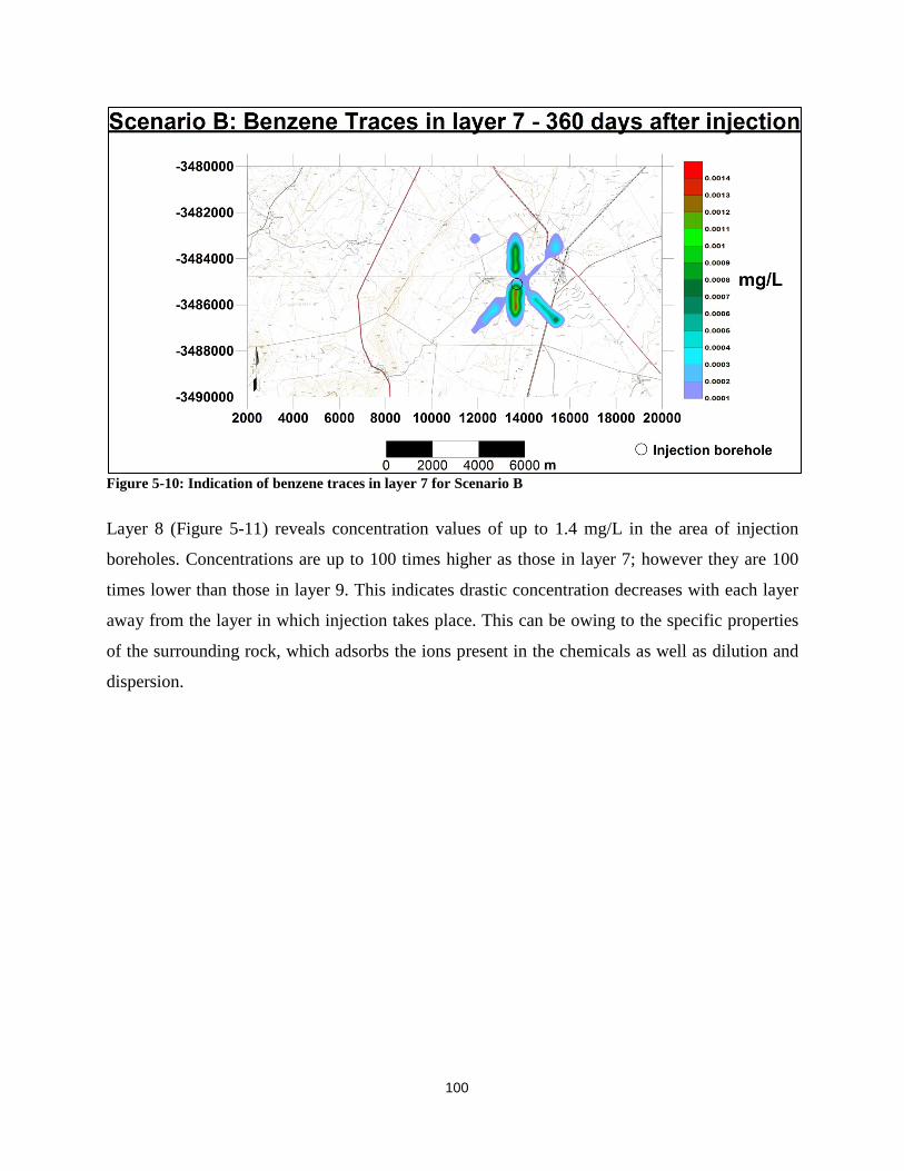
100






of the surrounding rock, which adsorbs the ions present in the chemicals as well as dilution and

dispersion.

101


Maximum concentration values of 320 mg/L are observed in layer 9 (Figure 5-12). The highest

concentrations of benzene are encountered around the injection locations. Concentrations

decrease with distance from injection sites. The pattern of concentrations that can be observed in

Figure 5-12 is due to horizontal fractures created during the fracturing process, via which the

fracking fluid flows. This may be primarily due to the fact that groundwater and contaminants

which follows groundwater will follow the path of least resistance as stated by Palmer (1996).

102


103

Scenario C

Indication of rises in water levels directly after injection (Figure 5-13) is indicated below. The

behavior of water levels in the central injection borehole over time is indicated in Figure 5-14.

The concentration values in various model layers follow thereafter (Figure 5-15 – Figure 5-18).

It can be observed that benzene traces are present in all the layers of the model.

104

Figure 5-13: Rise in Hydraulic heads in Layer 8 directly after injection for Scenario C

Minimal increases in water levels are observed in layers 1 to 7, 2 days after injection. Minimal



105




water levels.

Water levels over time in the central injection borehole are indicated in Figure 5-14. The water

level increases during to injection period and then with time starts decreasing. The pre-injection

water levels were not reached within the 360 days for which the model was run.

Figure 5-14: Change in water level in injection borehole over time for Scenario C


Benzene concentrations of up to 0.028 mg/L are observed in layer 1 after 360 days of injection

(Figure 5-15). This can be due to the injection method and the hydraulic conductivities of the

layer being higher than the deeper layers, thereby allowing benzene to enter the aquifer.

0 2 4 6 8

10 12 14 16

0 50 100 150 200 250 300 350 400

Chan

ge in

wat

er le

vels

(m)

Time (days)

Scenario C: Change in water level in injection borehole

106

Figure 5-15: Indication of benzene traces in layer 1 for Scenario C

Traces of benzene in the second layer reach a maximum of 0.0023 mg/L. Layers 3 to 6 have

concentration values of less than 3 x 10-5 mg/L. These values are all lower than the guideline

values discussed in Chapter 6.

107

Maximum concentrations of 0.03 mg/L are observed in layer 7 (Figure 5-16). Considering the

concentration increase in each layer, the pattern of higher concentration with depth becomes

clear, which signifies that fracking fluid injection takes place in the lowest layer and chemicals

disperse upward with time.






of the surrounding rock, as well as dilution and dispersion.

108


Concentration values of up to 340 mg/L are observed in layer 9 (Figure 5-18). The highest

concentrations of benzene are encountered around the injection locations. Concentrations

decrease with distance from injection sites. The pattern of concentrations that can be observed in

Figure 5-18 is due to horizontal fractures created during the fracturing process, via which the

fracking fluid flows. This may be primarily due to the fact that groundwater and contaminants

which follows groundwater will follow the path of least resistance as stated by Palmer (1996).

109


110

CHAPTER 6: DISCUSSION

Results for all the different chemicals used in the fracking fluid for this study, indicate there is a

chance of groundwater pollution, subsequent to fracking processes.

Corresponding results for methanol, with the highest concentration as well as all the chemicals

which have been modelled in this study with lower concentrations, confirm the presence of

varying concentrations in the surface layer of the model after a period of 360 days. Though

concentration values are within the national thresholds for drinking water, traces of chemicals

injected during fracking are proven to be present in the first layer and in all other layers above

that in which the fracturing takes places. It can be observed that benzene traces are present in all

the layers of the model. Threshold values for benzene are compared to concentrations of each

scenario in Sections 6.1; 6.2 and 6.3, respectively. This increases the possibility for chemicals to

be abstracted via boreholes for domestic, irrigation and other purposes. The influence of

fractures and the properties of the rocks in each specific layer are contributing factors that might

have the differing concentrations in the different layers as a result.

Water level changes were identified for all the scenarios. Changes in water levels in injection

boreholes over time were observed. The results indicated that water levels increased directly

after injection and thereafter decrease with time.

The change in water levels was highest for Scenario C and may be due to the multiple injection

boreholes present in this scenario which had greater volumes of water injected.

Increases in water levels over the whole area may have taken place as this is the case in the

injection boreholes, however the lower increases in Scenario B signifies the migration potential

closer dolerite intrusions is higher and therefore the greater increases in Scenario A and C.

Water level changes are very little over time and water levels do not drop back to initial levels in

the course of 360 days.

The geology and presence of numerous fractures, dykes and sills can influence the movement of

water. This is a serious factor that should be considered in fracking projects due to the fact that

not all chemicals used in fracking fluids are disclosed and only certain chemicals present in the

111

average fracking fluid with known concentrations, were used in this study. This emphasises the

conservativeness of this study and thus also the intensified awareness that should be kept when

projects in the Karoo are considered.

A separate discussion for the different scenarios follows, in order to indicate the different

findings for each:

6.1 Scenario A

Pollutant transport modelling for Scenario A reveals results which indicate that chemicals

injected at 3000 mbgl, reveal that traces of benzene are present in all layers; it also is present in

concentrations that exceed drinking water limits for benzene, in some places.

Table 6-1: Drinking water standards threshold value compared to benzene concentrations in all the layers of the model for Scenario A

National Primary Drinking Water Standards (WRWC, 2014)

Maximum Benzene Concentrations simulated in each layer for Scenario A (mg/L)

BENZENE Concentration at Point of Injection: 313.2 mg/L

MCLG (mg/L)

MCL (mg/L)

Potential Health Effects from Ingestion of Water:

Layer 1 0.015 Layer 2 Below MCL Layer 3 Below MCL Layer 4 Below MCL Layer 5 Below MCL Layer 6 Below MCL

0 0.005 Cancer Layer 7 0.0017 Layer 8 1.9 Layer 9 320

Where

Maximum Contaminant Level Goal (MCLG) – “The maximum level of a contaminant in

drinking water at which no known or anticipated adverse effect on the health effect of persons

would occur, and which allows for an adequate margin of safety. MCLGs are non-enforceable

public health goals” (Water Research Watershed Centre (WRWC), 2014).

112

Maximum Contaminant Level (MCL) – “The maximum permissible level of a contaminant in

water which is delivered to any user of a public water system. MCLs are enforceable standards.

The margins of safety in MCLGs ensure that exceeding the MCL slightly does not pose

significant risk to public health” (WRWC, 2014).

The results thus prove that migration of chemicals injected in fracking may influence the quality

of water resources. It may also pose health risks for exposed users due to concentrations that are

higher than the limits indicated by national authorities (WRWC, 2014). Scenario A represented a

single drilling pad with horizontal fracking which is located close to a dolerite dyke and the

matrix contains fractures in the shale layer caused by fracturing as well as natural fractures

ranging between 1 and 30 m in length. The results indicate that pollutant transport and water

level rises are a probability in an area in which dolerite dykes and natural fractures are present.

6.2 Scenario B

Traces of benzene are present in all layers 360 days subsequent to the fracturing injection period;

regardless of the fact the location of the injection borehole in this scenario further from a dyke

and other dolerite intrusions. The result for this scenario suggests that the presence of a injection

borehole close to a dyke is not the determining factor for pollutant migration.

Table 6-2: Drinking water standards threshold value compared to benzene concentrations in all the layers of the model for Scenario B

National Primary Drinking Water Standards (WRC, 2014)

Maximum Benzene Concentrations simulated in each layer for Scenario B (mg/L)


MCLG (mg/L)

MCL (mg/L)




113

6.3 Scenario C

Pollutant traces in all layers are also revealed in the results for Scenario C, where fracking has

fully commenced and the whole area is utilized for fracking borehole pads. Results indicate that

pollutants migrated from 3000 mbgl upwards in the course of the 360 days. However, it will be

recommend that future studies include models to simulate longer time periods after injection

periods.

Table 6-3: Drinking water standards threshold value compared to benzene concentrations in all the layers of the model for Scenario C

National Primary Drinking Water Standards (WRC, 2014)

Maximum Benzene Concentrations simulated in each layer for Scenario C (mg/L)


MCLG (mg/L)

MCL (mg/L)




The results prove that injected chemicals can migrate into the aquifer if boreholes are not cased

correctly. The presence of chemical traces in the surface layer should be considered as a potential

environmental impact due to unknown chemicals and their concentrations included in typical

fracking fluids that are not disclosed to the public.

The health risks that benzene as part of a fracking fluid, poses if ingested by an average human

being by means of abstraction from shallow aquifers are quantified below. Considering the

potential health risk indicated in Tables 6.1; 6.2 and 6.3, the carcinogenic risk will be quantified

for the benzene results.

Assumptions made for health risk quantification:

• Average adult weight: 70kg

114

• Intake of water per day: 2 litres per person • Average human lifetime: 70 years • Direct exposure (oral) to groundwater is considered. Indirect pathways are not allowed

for.

Equations specified in the EPA “Risk assessment Guidance for Superfund” (EPA, 1989) are used

as a base for equations used in order to determine the risks related to exposure to contaminated

groundwater. The total dose of a substance that a human will be exposed to has to be determined:

Dose = C x IR x ED

Where

Dose = Total dose

C = Maximum concentration

IR = Average intake rate

ED = Exposure duration

The maximum concentration overall concentration of the layers are used in the Dose equation in

order to account for all shallow aquifer and borehole water that can be exposed to users.

Scenario A

Maximum concentration observed in layers 1 to 4 for Scenario A is 0.015 mg/L

Thus Dose = C x IR x ED

= (0.015 mg/L) x (2 L/day) x (365 days)

= 10.95 mg

The average human lifetime is use to determine the carcinogenic risk assessment. The lifetime

average daily dose (LADD) is calculated as follows:

LADD = Total Dose BW × ED

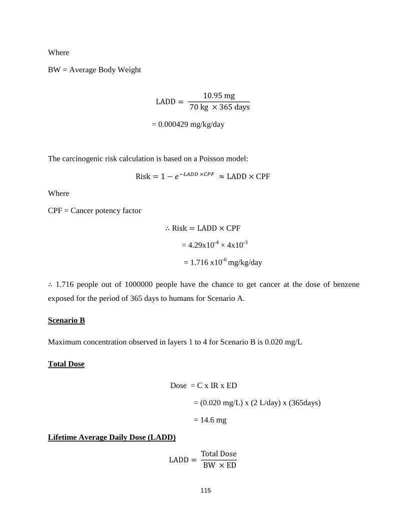
115

Where

BW = Average Body Weight

LADD = 10.95 mg

70 kg × 365 days

= 0.000429 mg/kg/day

The carcinogenic risk calculation is based on a Poisson model:

Risk = 1 − 𝑒−𝐿𝐴𝐷𝐷 ×𝐶𝑃𝐹 ≈ LADD × CPF

Where

CPF = Cancer potency factor

∴ Risk = LADD × CPF

= 4.29x10-4 × 4x10-3

= 1.716 x10-6 mg/kg/day

∴ 1.716 people out of 1000000 people have the chance to get cancer at the dose of benzene

exposed for the period of 365 days to humans for Scenario A.

Scenario B

Maximum concentration observed in layers 1 to 4 for Scenario B is 0.020 mg/L

Total Dose

Dose = C x IR x ED

= (0.020 mg/L) x (2 L/day) x (365days)

= 14.6 mg

Lifetime Average Daily Dose (LADD)


116

LADD = 14.6 mg

70 kg × 365 days

= 0.000571 mg/kg/day

Carcinogenic Risk:



= 5.71x10-4 × 4x10-3

= 2.285x10-6 mg/kg/day


exposed for the period of 365 days to humans for Scenario B.

Scenario C

Maximum concentration observed in layers 1 to 4 for Scenario C is 0.028 mg/L

Total Dose

Dose = C x IR x ED

= (0.028 mg/L) x (2 L/day) x (365 days)

= 19.6 mg

Lifetime Average Daily Dose (LADD)


LADD = 19.6 mg

70 kg × 365 days

= 0.000767 mg/kg/day

Carcinogenic Risk:



117

= 7.67x10-4 × 4x10-3

= 3.068 x10-6 mg/kg/day


exposed for the period of 365 days to humans for Scenario C.

By examining the carcinogenic health risk of benzene, it is evident that benzene would pose a

health risk in the study area for water users.

118

CHAPTER 7: CONCLUSION

Hydraulic fracturing was developed as a resource in order to provide abundant energy supplies

which will ultimately assist in an economically growing country. However, water is also a very

important resource that should be protected as it is at risk and starting to become endangered and

face extinction due to over exploitation and irresponsibility. Although the fracking process was

developed to benefit those who utilize it, concerns are increasingly arising regarding fracking

due to possible environmental impacts that have been identified, one being the impacts fracking

holds for the groundwater systems of the Karoo. In this study, the possibility of pollutant

transport in the subsurface towards shallow aquifers has been investigated by means of

numerical modelling.

The influence that the fracking fluid might have was the primary investigation as chemicals used

in the fracking fluid were individually modelled to ultimately determine the probability for each

chemical species to migrate to the surface. This was also done in order observe a change in

concentration values of each species throughout each layer of the model.

As the fracking fluid consists of large volumes of water, the water injected at 3000 mbgl was

also modelled. This gave an indication of water level changes when results of new water levels

were compared with original water levels.

Secondary research questions (as mentioned in Section 1.3) which may arise from the

fundamental research question are: “Is subsurface migration of fluids to drinking water resources

possible, and what is the cause for this to potentially occur?”

The results of this study did not verify the movement of pollution to shallow aquifers.

Concentrations of benzene for Layer 1 in each scenario exceed the permitted concentrations in

drinking water at certain points and hold a carcinogenic health risk for all users of groundwater

from this area. This was due to the injection method, higher hydraulic conductivities in the first

layer and no borehole casing being taken into account. This suggests that subsurface migration of

chemicals and rising water levels in groundwater systems is indeed a factor to consider in the

decision making of fracking implementation in South Africa. With the Karoo geology and

associated preferential pathways produced by dolerite intrusions, the risk of pollutant transport to

119

water resources utilized by human, plant and animal, is one that does exist. Geological features

do indeed play a role in subsurface migration. Man-made features such as boreholes may also

promote subsurface migration due to abstraction from deep aquifers. The hypothesis of fracking

having an influence on the groundwater systems and its chemistry and thus also the surrounding

environment, made in this study, is proven by the results.

All the scenarios that were modelled in this study for all the different chemicals with their

specific concentrations produce similar results for pollutant transport and a change in water

levels. Although concentrations and water levels differ for each chemical and each scenario, an

overall consistent conclusion can be drawn: pollutant transport towards the surface and changes

in water levels after fracking fluid injection.

Questions that were raised in Section 1.3 include: “What are the possible impacts of borehole

injection on water resources, specifically the Karoo groundwater systems for this study?” “Is

subsurface migration of fluids or gases to drinking water resources possible, and what is the

cause for this to potentially occur?” After the results were conceptualized, these questions could

be addressed:

Results indicate that borehole injection of fracking fluids could have pollutant transport in the

groundwater systems of the Karoo as an effect. This means that fracking would most possibly

have an impact on the groundwater systems as chemicals interact with the geology and water

resources in its flow path (refer to Section 2.1.2 – 2.1.4). As results for three different scenarios

revealed similar results, it can be concluded that major geological features such as faults and

fractures, dykes and other intrusions do not primarily dictate whether pollutant transport or an

increase in water levels will occur, however they do influence the rate of movement and in some

cases the direction thereof.

The main conclusion that can be made considering the results obtained for the different scenarios

from this study is that groundwater systems of the Karoo will be impacted by fracking processes.

An overview of other activities in the Karoo that might be influenced by fracking is given in

Appendix G.

120

Summary

The baseline study revealed that water resources are limited and that the geology of the Karoo is

complex, along with dolerite intrusions which could possibly serve as preferential pathways for

fluid migration. This emphasized the importance of water conservation and therefore an

investigation on the transport and flow of the injected fluid was done to determine the probability

of fluid migration in the specific study area. Results obtained from numerical modelling would

suggest whether fracking might have an impact on the groundwater systems of the Karoo.

Numerical modelling of a model which represents the study area of this study produced results

which indicate the probability for pollutant transport in the groundwater systems of the Karoo.

The conclusion is made that fracking will indeed have an impact on the groundwater systems of

the Karoo.

Future Recommendations

As there are various factors regarding fracking that might have major impacts on the

environment, future recommendations are made based on existing concerns. A similar study than

this could be done once more chemicals and their concentrations present in fracking fluids are

disclosed in the future. Observation periods of more than 360 days should be included in order to

obtain an idea of the increases and decreases of water levels as well as concentrations of

chemicals over time for future reference. A detailed field study of the area is also recommended

in order to obtain more site specific data. This includes the drilling of deep boreholes where

studies and investigations are focused. As fracking is a new process to be implemented in South

Africa, studies on concerns such as surface spills and water use raised by an institution like the

U.S. Environmental Protection Agency (Figure 1-1) should be done on site specific areas in

South Africa in order to determine possible results for the concerns in South Africa specifically.

Studies on the integrity of borehole construction should also be done in order to determine the

probability for borehole and casing stability failure in the fracturing process which could cause

direct pollution to shallow aquifers when fracking fluid is injected. The effect of different

injection techniques should also be investigated.

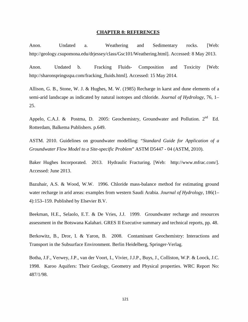
121

CHAPTER 8: REFERENCES

Anon. Undated a. Weathering and Sedimentary rocks. [Web:

http://geology.csupomona.edu/drjessey/class/Gsc101/Weathering.html]. Accessed: 8 May 2013.

Anon. Undated b. Fracking Fluids- Composition and Toxicity [Web:

http://sharonspringsspa.com/fracking_fluids.html]. Accessed: 15 May 2014.

Allison, G. B., Stone, W. J. & Hughes, M. W. (1985) Recharge in karst and dune elements of a

semi-arid landscape as indicated by natural isotopes and chloride. Journal of Hydrology, 76, 1–

25.

Appelo, C.A.J. & Postma, D. 2005: Geochemistry, Groundwater and Pollution. 2nd Ed.

Rotterdam, Balkema Publishers. p.649.

ASTM. 2010. Guidelines on groundwater modelling: “Standard Guide for Application of a

Groundwater Flow Model to a Site-specific Problem” ASTM D5447 - 04 (ASTM, 2010).

Baker Hughes Incorporated. 2013. Hydraulic Fracturing. [Web: http://www.mfrac.com/].

Accessed: June 2013.

Bazuhair, A.S. & Wood, W.W. 1996. Chloride mass-balance method for estimating ground

water recharge in arid areas: examples from western Saudi Arabia. Journal of Hydrology, 186(1–

4):153–159. Published by Elsevier B.V.

Beekman, H.E., Selaolo, E.T. & De Vries, J.J. 1999. Groundwater recharge and resources

assessment in the Botswana Kalahari. GRES II Executive summary and technical reports, pp. 48.

Berkowitz, B., Dror, I. & Yaron, B. 2008. Contaminant Geochemistry: Interactions and

Transport in the Subsurface Environment. Berlin Heidelberg, Springer-Verlag.

Botha, J.F., Verwey, J.P., van der Voort, I., Vivier, J.J.P., Buys, J., Colliston, W.P. & Loock, J.C.

1998. Karoo Aquifers: Their Geology, Geometry and Physical properties. WRC Report No:

487/1/98.

http://www.mfrac.com/


http://www.sciencedirect.com/science/journal/00221694/186/1

http://www.sciencedirect.com/science/journal/00221694/186/1

122

Botha, J. F. & Cloot, A. H. J. 2004. Karoo aquifers, deformations, hydraulic and mechanical

properties. Research Report No.936/1/04. Water Research Commission of South Africa, Pretoria.

Bredenkamp, D.B., Botha, L.J., Van Tonder, G.J. & Van Rensburg, H.J. 1995. Manual on

Quantitative Estimation of Groundwater Recharge and Aquifer Storativity, Water Research

Commission Report TT73/95, Pretoria, South Africa. (ISBN 1 86845 1763).

Brownell, M. 2008. Gas well drilling and development: Marcellus shale. Susquehanna River

Basin Commission. [Web: /http: //www. srbc.net/whatsnew/docs/Marcellusshale61208ppt.PDF].

Accessed: 25 November 2012.

Bucas, K. 2006. Natural and anthropogenic influences on the water quality of the Orange River,

South Africa. Minor Dissertation for the degree Master of Science at the University of

Johannesburg.

Business Report. 2012. SA gets a major look-in on SKA’s Karoo telescope project. [Web:

http://www.iol.co.za/business/business-news/sa-gets-a-major-look-in-on-ska-s-karoo-telescope-

project-1.1305569]. Accessed: 1 March 2013.

Cairncross, B. 2004. Field guide to Rocks and Minerals of Southern Africa. 1st Ed. Cape Town,

Struik Publishers.

CARBO Ceramics. 2011. Fracpro®: The world’s leading fracture stimulation software. [Web:

http://www.carboceramics.com/fracpro/]. Accessed: June 2013.

Chevallier, L., Gibson, L. A., Nhleko, L. O., Woodford, A. C., Nomquphu, W. & Kippie, I.

2004a. Hydrogeology of fractured-rock aquifers and related ecosystems within the Qoqodala

dolerite ring and sill complex, Great Kei Catchment, Eastern Cape. Research Report

No.1238/1/04. Water Research Commission of South Africa, Pretoria.

Chevallier, L., Nhleko, L., Wheeler, W. & Woodford, A. C. 2004b. Exploration drilling and

aquifer testing at Qoqodala dolerite sill and ring complex, Eastern Cape, South Africa.

Confidential Report. Council for Geoscience.

http://www.iol.co.za/business/business-news/sa-gets-a-major-look-in-on-ska-s-karoo-telescope-project-1.1305569

http://www.iol.co.za/business/business-news/sa-gets-a-major-look-in-on-ska-s-karoo-telescope-project-1.1305569

123

Chevallier, L., Goedhart, M. & Woodford, A.C. 2001. The influences of dolerite sill and ring

complexes on the occurrence of groundwater in the Karoo fractured aquifers: A morpho-tectonic

approach.WRC Report No. 937/1/01.

Chevallier, L. & Woodford, A. 1999. Morpho-tectonics and mechanism of emplacement of the

dolerite rings and sills of the western Karoo, South Africa. South African Journal of Geology,

102(1): 43-54.

Cobbing, J., Adams, S., Dennis, I. & Riemann, K. 2013. Assessing and Managing Groundwater

in different Environments. CRC Press, Taylor & Francis Group, London, UK. p.259.

Coetzee, M.S. 2008. Sedimentary rocks: South African Geology. [Personal communication,

2008]. NWU Potchefstroom Campus.

Colborn, T., Kwiatowski, C., Schultz, K., & Bachran, M. 2011. Natural Gas Operations from a

Public Health Perspective, Human and Ecological Risk Assessment: An International Journal,

17(5): 1039–1056.

Connectflow, Undated. Connectflow. [Web: http://www.connectflow.com/]. Accessed: June

2013.

Consortium for Spatial Information (CGIAR-CSI). 2013. Topographical data for Victoria West,

South Africa.[Web: http://www.cgiar-csi.org/data/srtm-90m-digital-elevation-database-v4-1].

Accessed: August 2013.

Council for Geoscience. 2014. SA Geology and Karoo Aquifer Data. [Web:

http://www.geoscience.org.za/1-1-000-000-geological-data]. Accessed: November 2014.

Council for Geoscience. 2013. Geological data for South Africa and D61E [Shape files

extracted]. June 2013

Council for Geoscience. 1997. 1:1 000 000 Geological Map of the Republic of South Africa and

the Kingdoms of Lesotho and Swaziland.





124

Das, D.B. 2002. Hydrodynamic modelling for groundwater flow through permeable reactive

barriers. Hydrological Processes. 16: 3393–3418.Department of Environmental Protection

Bureau of Oil and Gas Management. 2010. Chemicals Used in the Hydraulic Fracturing Process

in Pennsylvania. [Web: http://marcellusdrilling.com/2010/06/list-of-78-chemicals-used-in-

hydraulic-fracturing-fluid-in-pennsylvania/]. Accessed: 15 May 2014.

Department of Mining. 1976. Delfstowwe van die Republiek van Suid-Afrika. 5th Ed. Pretoria,

Staatsdrukker.

Department of Water Affairs (DWA). 2013a. Rivers shape file. [Web:

https://www.dwaf.gov.za/iwqs/gis_data/river/rivs500k.aspx]. Accessed: June 2013.Department

of Water Affairs (DWA). 2013b. Groundwater chemistry data [e-mail]. 17 April 2013; 8 August

2013.

Department of Water Affairs (DWA). 2013c. Borehole data [NGA Files Extracted]. 7

September 2013.

Department of Water and Environmental Affairs (DWA). 2009. Development of an

Integrated Water Quality Management Strategy for the Upper and Lower Orange Water

Management Areas, Desktop Catchment Assessment Study: Lower Orange Water

Management Area (WMA 14). Report No. 2.2 (P RSA D000/00/7909/3). 1st Ed.

August 2009.

Duffield, G.M. 2014. Representative Values of Hydraulic Properties. HydroSOLVE, Inc. 1998-

2014. [Web: http://www.aqtesolv.com/aquifer-tests/aquifer_properties.htm]. Accessed: 24

November 2014.

Duncan, A.R. & Marsh, J.S. 2006. The Karoo Igneous Province. In: Johnson, M.R.,

Anhaeusser, C.R. & Thomas, R.J. (Eds.). The Geology of South Africa, p.461-520. Geological

Society of South Africa, Marshalltown. Council for Geoscience, Pretoria.

DWA: see Department of Water Affairs

http://marcellusdrilling.com/2010/06/list-of-78-chemicals-used-in-hydraulic-fracturing-fluid-in-pennsylvania/

http://marcellusdrilling.com/2010/06/list-of-78-chemicals-used-in-hydraulic-fracturing-fluid-in-pennsylvania/

https://www.dwaf.gov.za/iwqs/gis_data/river/rivs500k.aspx

http://www.aqtesolv.com/hydrosolve/default.htm

125

Earthworks. 2012. Hydraulic Fracturing 101. [Web:

http://www.earthworksaction.org/issues/detail/hydraulic_fracturing_101#.VGCOq-kcS00 ].


Eby, G.N. 2004. Principles of Environmental Geochemistry. Belmont, USA, Brooks/Cole

CENGAGE Learning. p.147-148.

EPA. 1989. Risk Assessment Guidance for Superfund, Volume I, Human Health Evaluation

Manual (Part A). Interim Final EPA/540/1-89/002. Washington, D.C.

EPA. 2011. Groundwater. [Web: http://www.epa.gov/superfund/students/clas_act/haz-

ed/ff_05.htm]. Accessed: 21 April 2014.

Eriksson, E. and Khunakasem, V., 1969. Chloride concentration in groundwater, recharge rate

and rate of deposition of chloride in the Israel coastal plain. Journal of Hydrology, 7, 178-197.

Fetter, C.W. Jr. 1988. Applied Hydrology. 2nd Ed. New York, C. E. Merrill Publishing Co.

p.592.

FEFLOW. 2012. FEFLOW. [Web: http://www.feflow.info/]. Accessed: 23 May 2013.

Finewood, M.H. & Stroup, L.J. 2012. Fracking and the Neoliberalization of the Hydro-Social

Cycle in Pennsylvania’s Marcellus Shale. Universities Council on Water Resources. Journal of

Contemporary Water Research & Education, 147: 72-79.

Fitts, C.R. 2013. Groundwater Science. 2nd Ed. Oxford, UK. Elsevier, Inc.

Flores, R.M. 2014. Coal and Coalbed Gas: Fueling the Future. 1st Ed. San Diego, CA, USA.

Elserivier, Inc. ISBN: 9780123969729

Fortson, L. A., Yatzor, B. & Bank, T. 2011. Physical and Chemical Associations of Uranium

and Hydrocarbons in the Marcellus Shale. In Proceedings of’ Northeastern (46th Annual) and

North-Central (45th Annual) Joint Meeting. Geological Society of America; University at

Buffalo.

http://www.feflow.info/

126

Fouty, S.C.1989. Chloride Mass Balance as a method for determining long-term Groundwater

Recharge Rates and Geomorphic-Surface Stability in Arid and Semi-Arid Regions Whisky Flat

and Beatty, Nevada. Arizona: The University of Arizona. (Manuscript – MSc.).

FRACMAN. 2013. Fracman Software. [Web:

http://fracman.golder.com/software/software.asp]. Accessed: 1 June 2013.

Gieske, A., 1992. Dynamics of groundwater recharge: A case study in semi-arid

EasternBotswana. Amsterdam: Vrije Universiteit. (Thesis – Ph.D). 290 pp.

Golder Associates. 2011. Environmental Management Plan (EMP): South Western Karoo Basin

Gas Exploration Application: Central Precinct. Shell Exploration Company B.V. Report No.

12800-10534-29.

Grotzinger, J., Jordan, T.H., Press, F. & Raymond, S. 2007. Understanding earth. 5th Ed. New

York: W. H. Freeman and Company. p.409.

GroundwaterGo. 2011. DNAPL modeling: UTCHEM vs MODFLOW. Part 3 – Comparison of

numerical methods. [Web: http://www.groundwatergo.com/blog/dnapl-modeling-utchem-vs-

modflow-part-3-comparison-of-numerical-methods/]. Accessed: 22 May 2013.

GWPC & IOGCC. 2014a. Fracfocus, Hydraulic Fracturing: The Process. [Web:

http://fracfocus.org/hydraulic-fracturing-how-it-works/hydraulic-fracturing-process]. Accessed:

10 November 2014.

GWPC & IOGCC. 2014b. Fracfocus, What chemicals are used. [Web:

http://fracfocus.org/chemical-use/what-chemicals-are-used]. Accessed: 10 November 2014.

GWPC & IOGCC. 2014c. Fracfocus, Chemical use. [Web: https://fracfocus.org/chemical-use].


GWPC & IOGCC. 2014. Fracfocus, Chemical Use in Hydraulic Fracturing. [Web:

http://fracfocus.org/water-protection/drilling-usage]. Accessed: 10 November 2014.

127

Halliburton. 2014. Pennsylvania WaterFrac Formulation: Marcellus Shale. [Web:

http://www.halliburton.com/public/projects/pubsdata/hydraulic_fracturing/fluids_disclosure.html

]. Accessed: 10 November 2014.

Harbaugh, A.W., E.R. Banta, M.C. Hill, & McDonald, M.G. 2000. Modflow-2000, the U.S.

Geological Survey modular ground-water model—User guide to modularization, concepts and

the ground-water flow process. Open-File Report 00-92. Reston, Virginia, U.S. Geological

Survey.

Harper, J. 2008. The Marcellus Shale-an Old ‘‘New’’ gas reservoir in Pennsylvania.

Pennsylvania Geology. 38: 2–12.

Hayden, J. & Pursell, D. 2005. The Barnett Shale: Visitors Guide to the Hottest Gas Play in the

US. Pickering Energy Partners Inc. [Web:

http://www.tphco.com/Websites/tudorpickering/Images/Reports%20Archives/TheBarnettShaleR

eport.pdf]. Accessed: January 2015.

Hem, J.D. 1989. Study and Interpretation of the Chemical Characteristics of Natural Water. 3rd

Ed. United States Geological Survey. Water Supply Paper 2254.

Hill, R. S. 1993. The geology of the Graaff-Reinet area. Explanation of Sheet 3224 (scale 1:250

000). Geological Survey of South Africa: 31.

Horwitt, D. 2009. Drilling Around the Law. Washington, D.C., Environmental Working Group.

Hsieh, P.A. 2011. Application of MODFLOW for Oil Reservoir Simulation During the

Deepwater Horizon Crisis. Groundwater. 49(3): 319 – 323.

Huizenga, J.M. 2011a. Characterisation of the inorganic chemistry of surface waters in South

Africa. Water SA. 37: 401-410.

Huizenga, J.M. 2011b. Metamorphic Petrology and Geochemistry. [Personal communication,

2011]. NWU Potchefstroom campus.

128

IEA. 2012. Golden rules of a golden age of gas. World Energy Outlook. Special Report on

Unconventional Gas. Paris, France, International Energy Agency. p.143.

Johnson, M.R., Anhaeusser, C.R., & Thomas, R.J. 2006. The Geology of South Africa. 1st Ed.

Published jointly by the Geological Society of South Africa, Johannesburg, and the Council for

Geoscience, Pretoria. p.651- 656.

King, H. 2013. Shale. [Web: http://geology.com/rocks/shale.shtml]. Access: 12 February 2013.

Kinzelbach, W., Aeschbach, W., Alberich, C., Goni, I.B., Beyerle, U., Brunner, P., Chiang, W.-

H., Rueedi, J. & Zoellmann, K. 2002. A Survey of Methods for Groundwater Recharge in Arid

and Semi-arid regions. Early Warning and Assessment Report Series, UNEP/DEWA/RS.02-2.

United Nations Environment Programme, Nairobi, Kenya. ISBN 92-80702131-3.

Lerner, D.N., Issar, A.S. & Simmers, I. 1990. Groundwater Recharge, A Guide to

Understanding and Estimating Natural Recharge. Int. Contributions to Hydrogeology

(IAH), Vol. 8, 1990, Verlag Heinz Heise, Germany, pp. 345.Lesage, S. & Jackson, R.E. 1992.

Groundwater contamination and analysis at hazardous waste sites. New York, Marcel Dekker,

Inc., 552 p.

Lindeque, A.S., Ryberg, T., Stankiewicz, J., Weber, M.H. & De Wit, M. J. 2007. South African

Journal of Geology, 110: 419-438.

Love, A. H. 2005. Fracking: The Controversy over its Safety for the Environment. Lafeyette,

CA: Johnson Wright, Inc.

Lüning, S. Undated. Black Shale Research. [Web: http://www.blackshale.com/]. Accessed: 13

February 2013.

Lurie, J. 1979. South African geology for mining, metallurgical, hydrological and civil

engineering. 2nd Ed. Johannesburg, McGraw-Hill Book Company. p.41-53.

Mao, X., Prommer, H., Barry, D.A., Langevin, C.D., Panteleit, B. & Li, L. 2006. Three-

dimensional model for multi-component reactivetransport with variable density groundwater

flow. Environmental Modelling & Software. 21: 615–628.

http://www.johnsonwright.net/newsletters/2011-December/Fracking-The_Controversy_Over_its_Safety_for_the_Environment.htm

129

MARS. Undated. MARS. [Web:

http://www.scientificsoftwaregroup.com/pages/detaileddescription.php?productsid=46].

Accessed: 9 July 2013.

McCarthy, T. & Rubidge, B. 2005. The story of earth and life. Cape Town, Struik Publishers.

p.317.

McCartney, M.P., Yawson, D.K., Magagula, T.F. & Seshoka, J. 2004. Hydrology and water

resources development in the Olifants River Catchment. Working Paper 76. Colombo, Sri Lanka:

International Water Management Institute (IWMI). [Web:

http://www.iwmi.cgiar.org/Publications/Working_Papers/working/WOR76.pdf]. Accessed: 8

December 2014.

McElreath, D. Undated. Comparison of Hydraulic Fracturing Fluids Composition with

Produced Formation Water following Fracturing – Implications for Fate and Transport.

Oklahoma City, Oklahoma, Chesapeake Energy Corporation. [Web:

http://water.epa.gov/type/groundwater/uic/class2/hydraulicfracturing/upload/comparisonofhfflui

dscompositionwithproducedformationwater.pdf]. Accessed: 13 October 2014.

Melton Wold. 2013. Great Karoo. [Web: http://www.meltonwoldsafaris.co.za/area/karoo.html].

Accessed: 19 March 2013.

Meybeck, M. 1985. How to establish and use world budgets of riverine materials. In Lerman,

A. & M. Meybeck (eds.): Physical and Chemical weathering in Geochemical Cycles. NATO ASI

Series. 251. Dordrecht, Kluwer Academic Publishers.

MIKE-SHE. Undated. GIS and water resource modelling at DHI. [Web:

http://www.crwr.utexas.edu/gis/gishyd98/dhi/mikeshe/Mshemain.htm]. Accessed: 23 May 2013.

Monroe, J.S., Wicander, R., Hazlett, R. 2007. Physical Geology: Exploring the Earth. 6th Ed.

Belmont, USA, Thomson Brooks. p.111

Moridis, G.J. & Pruess, K. 1997. Report by Ernest Orlando Lawrence Berkeley national

laboratory.T2SOLV: An Enhanced Package of Solvers for the TOUGH2 Family of Reservoir

http://www.scientificsoftwaregroup.com/pages/detaileddescription.php?productsid=46

130

Simulation Codes. Earth Sciences Division. [Web:

http://esd.lbl.gov/files/research/projects/tough/documentation/T2SOLV_Users_Guide.pdf].Acces

sed: 20 May 2013.

Myers, T. 2012. Potential Contaminant Pathways from Hydraulically Fractured Shale to

Aquifers. Ground Water. National GroundWater Association. 50(6): 872–882.

Norman, N. & Whitfield, G. 2006. Geological Journeys.1st Ed. Cape Town, Struik Publishers

and Council for Geoscience. p.176.

Palmer, C.M. 1996. Principles of Contaminant Hydrogeology, 2nd Ed. Boca Raton, Florida,

USA. CRC Lewis Publishers Inc.

Pretorius, J. 2012. A petrographical and geochemical investigation of four different South

African kimberlites, pertaining to a possible source for the dispersive character of diamond mine

tailings. Dissertation for Honours degree Baccaleurs Scientia at the North-West University,

Potchefstroom Campus, Potchefstroom.

Rahm, D. 2011. Regulating hydraulic fracturing in shale gas plays: The case of Texas. Energy

Policy 39: 2974–2981.

Reeves, D.M., Zhang, Y., Pohll, G., & Benson, D. 2008. FRACK: A Freeware Flow and

Transport Suite for Fractured Media. [Web:

http://www.dri.edu/images/stories/editors/mattreeves/MODFLOWmf2k8_FRACK.pdf].

Accessed: 3 June 2013.

Reservoir Engineering Research Program, Texas. 2000. Volume I: User's Guide for UTCHEM-

9.0: A Three-Dimensional Chemical Flood Simulator. Center for Petroleum and Geosystems

Engineering: The University of Texas at Austin.

Rowsell, D. M, & Swardt, A. M. J. 1976. Diagenesis in Cape and Karoo Sediments, South

Africa, and Its Bearing on Their Hydrocarbon Potential. Trans. Geological Society of South

Africa. 79: 81-145.

131

Rossouw, L., Avenant, M.F., Seaman, M.T., King,J.M., Barker, C.H., du Preez, P.J., Pelser, A.J.,

Roos, J.C., Van Staden, J.J., van Tonder, G.J. & Watson, M. 2005. Environmental Water

Requirements in Non-Perennial Systems. WRC Report No: 1414/1/05; ISBN No.: 1-77005-363-

8; Set No.: 1-77005-362-X.

Scanlon, B.R., Healy, R.W. & Cook, P.G. 2002. Choosing appropriate techniques for

quantifying groundwater recharge. In Theme issue on groundwater recharge (ed. B.R.Scanlon

and P.G. Cook), Journal of Hydrogeology, 10, 18-39.

Schlumberger. 2010. Fraccade: Fracturng design and evaluation software. [Web:

https://www.slb.com/~/media/.../fraccade_frac_design_software_ps.pdf]. Accessed: June 2013.

Schlumberger Limited. 2013. Petrel Geology & Modeling. [Web:

http://www.software.slb.com/products/platform/pages/petrel-geology-modeling-

software.aspx].Accessed: June 2013.

Schlumberger: Water Services. 2013. Groundwater Modeling Software: Visual MODFLOW

Flex. [Web: http://www.swstechnology.com/groundwater-modeling-software/visual-modflow-

flex?gclid=CPic7qSY8rYCFXDMtAodZVsAqQ]. Accessed: 20 May 2013.

Simcore Software, 2016. Simcore Software. [Web: www.simcore.com/pm8]. Accessed: 17

August 2016.

SKA South Africa. 2013. MeerKAT. [Web: www.ska.ac.za/meerkat/]. Accessed: 1 March

2013.

Soeder, D.J. 2010. The Marcellus Shale: Resources and reservations. Eos. 91 (32): 277.

South African Weather Service. 2013. Rainfall data for Victoria West [e-mail]. 26 April 2013.

Späth, A. 2010. Fracking up the Karoo. News24, 2010-09-15.

Spits, K. & Moreno, J. 1996. A Practical Guide to Groundwater and Solute Transport

Modeling. New York, John Wiley & Sons Inc.

http://www.uncertaintyes.org/index.php/en/software/petrel

132

Srinivasan,V., Clement, T.P. &. Lee, K.K. 2007. “Domenico Solution—Is It Valid?” Ground

Water. 45(2): 136–146.

StatSilk. 2014. South Africa Maps [Web: http://www.statsilk.com/maps/download-free-

shapefile-maps]. Accessed: November 2014.

Steyl, G., van Tonder, G.J. & Chevallier, L. 2012. State of the art: fracking for shale gas

exploration in south africa and the impact on water resources. Report to the Water Research

Commission from the University of the Free State and Council for Geoscience. [Web:

www.wrc.org.za]. Accessed: 31 January 2013.

Steyl, G. & van Tonder, G.J. 2013. Hydrochemical and Hydrogeological Impact of Hydraulic

Fracturing in the Karoo, South Africa, Effective and Sustainable Hydraulic Fracturing, Dr. Rob

Jeffrey (Ed.), ISBN: 978-953-51-1137-5, InTech, DOI: 10.5772/56310. [Web:

http://www.intechopen.com/books/effective-and-sustainable-hydraulic-

fracturing/hydrochemical-and-hydrogeological-impact-of-hydraulic-fracturing-in-the-karoo-

south-africa]. Accessed: January 2015.

Straterra, Natural Resources of New Zeeland. 2013. Chemicals used in fracking. [Web:

http://www.straterra.co.nz/Fracking%20chemicals]. Accessed: 9 April 2013.

Svensen, H., Jamtveit, B., Planke, S. & Chevallier, L. 2006. Structure and evolution of

hydrothermal vent complexes in the Karoo Basin, South Africa. Journal of the Geological

Society, 163(4): 671-682.

Taylor, D.M. & Taylor, S.K. 1997. Environmental uranium and human health. Reviews on

Environmental Health. University of Heidelberg: Institute of Pharmacology and Toxicology,

Germany. 12(3): 147-57.

Tenbus, F.J. & Fleck, W.B. 2001. Simulation of Ground-Water Flow and Transport of

Chlorinated Hydrocarbons at Graces Quarters, Aberdeen Proving Ground, Maryland. USGS:

Science foe a changing world. Water-Resources Investigations Report 01-4106. [Web:

http://pubs.usgs.gov/wri/wri01-4106/wrir-01-4106.pdf]. Accessed: 30 April 2013.

http://www.wrc.org.za/

http://jgs.geoscienceworld.org/search?author1=Henrik+Svensen&sortspec=date&submit=Submit

http://jgs.geoscienceworld.org/search?author1=Bj%C3%98rn+Jamtveit&sortspec=date&submit=Submit

http://jgs.geoscienceworld.org/search?author1=Sverre+Planke&sortspec=date&submit=Submit

http://jgs.geoscienceworld.org/search?author1=Luc+Chevallier&sortspec=date&submit=Submit

http://www.ncbi.nlm.nih.gov/pubmed/9406286

http://www.ncbi.nlm.nih.gov/pubmed/9406286

133

Toth, J. 1984. “The Role of Regional Gravity flow in the Chemical and Thermal Evolution of

groundwater”, First Canadian /American conference on Hydrogeology, Banff, Canada, National

Water Well Association, Dublin, OH. p.3-39.

TOUGH2-MP. 2007. TOUGH2-MP. [Web: http://www.tough2.com/index2.html]. Accessed:

24 May 2013.

Tourtelot, H.A. 1979. Black Shale—It’s deposition and diagenesis 1.Clays and Clay Minerals.

27(5): 313-321.

United Nations Environment Programme (UNEP) Global Environmental Alert Service (GEAS).

2013. Gas fracking: Can we safely squeeze the rocks ?. Environmental Development, Elsevier.

[Web: http://ac.els-cdn.com/S2211464512001480/1-s2.0-S2211464512001480-

main.pdf?_tid=c5a06f9a-a28b-11e2-aba3-

00000aab0f6c&acdnat=1365673377_ce358f486f7966a180f92712fbd1957f ]. Accessed: 10 April

2013.

United Nations Environment Programme (UNEP). 2010. Clearing the Waters: A focus on water

quality solutions. ISBN: 978-92-807-3074-6. [Web:

http://www.unep.org/PDF/Clearing_the_Waters.pdf]. Accessed: January 2015.

U.S. Environmental Protection Agency: Ground Water and Ecosystems Restoration. 2013.

Centre for Subsurface Modelling Support Research. [Web: http://www.epa.gov/ada/csmos/].

Accessed: 24 May 2013.

U.S. Environmental Protection Agency: Ground Water and Ecosystems Restoration. 2012a.

Potential Limitations of Four Domenico-Based Fate and Transport Models. [Web:

http://www.epa.gov/ada/csmos/domenico.html]. Accessed: 24 May 2013.

U.S. Environmental Protection Agency, United States. 2012b. Study of the Potential Impacts of

Hydraulic Fracturing on Drinking Water Resources. Washington, D.C., U.S. Environmental

Protection Agency: Office of Research and Development.

U.S. Environmental Protection Agency, United States. 2012c. Uranium. [Web:

http://www.epa.gov/radiation/radionuclides/uranium.html#change]. Accessed: 12 February 2013.

http://www.epa.gov/ada/csmos/domenico.html

http://www.epa.gov/radiation/radionuclides/uranium.html#change

134

U.S. Environmental Protection Agency, United States. 2011. Draft Plan to Study the Potential

Impacts of Hydraulic Fracturing on Drinking Water Resources. Washington, D.C., U.S.

Environmental Protection Agency. 2013.

USGS. 2005. MODFLOW-2005, The U.S. Geological Survey Modular Ground-Water Model–

the Ground-Water Flow Process. U.S. Geological Survey Techniques and Methods 6-A16. U.S.

Department of the Interior and U.S. Geological Survey. [Web:

http://pubs.usgs.gov/tm/2005/tm6A16/]. Accessed: 15 November 2012.

USGS. 2013. SUTRA. [Web: http://water.usgs.gov/nrp/gwsoftware/sutra/sutra.html].


USGS. 2014a. Environmental Health- Toxic Substances. [Web:

http://toxics.usgs.gov/definitions/lnapls.html]. Accessed: 24 April 2015.

USGS. 2014b. Chloride Mass Balance in Streams to Estimate Recharge. [Web:

http://water.usgs.gov/ogw/gwrp/activities/cl-mass-balance.html]. Accessed: 14 May 2015.

USGS. Undated. Natural Processes of Ground-Water and Surface-Water Interaction: The

Hydrologic Cycle and Interactions of Ground Water and Surface Water. [Web:

http://pubs.usgs.gov/circ/circ1139/pdf/part1a.pdf]. Accessed: 21 April 2014.

Vaidyanathan, G. 2012. Astronomers relaxed about fracking near South African telescopes.

[Web: http://blogs.nature.com/news/2012/09/astronomers-relaxed-about-fracking-near-south-

african-telescopes.html]. Accessed: 4 February 2013.

Van Tonder, G. 2012. Karoo Groundwater Atlas. [Web: http://s03.static-

shell.com/content/dam/shell/static/zaf/downloads/media/karoo-groundwateratlas.pdf]. Accessed:

19 March 2013.

Van Wyk, E., Van Tonder, G.J. & Vermeulen, D. 2011. Characteristics of local groundwater

recharge cycles in South African semi-arid hard rock terrains - rainwater input. Water SA

[online]. 2011, vol.37, n.2, pp. 147-154. ISSN 1816-7950.

135

van Zijl, J.S.V. 2006. Physical characteristics of the Karoo sediments and mode of

emplacement of the dolerites. South African Journal of Geology, September 2006, v. 109,no.3; p.

329-334.

Water Research Watershed Centre. 2014. EPA Drinking Water Standards - Water Research

Center. [Web: http://www.water-research.net/index.php/standards/primary-standards].


Wels, C., Mackie, D. & Scibek, J. 2012. Guidelines for Groundwater Modelling to Assess

Impacts of Proposed Natural Resource Development Activities. British Columbia Ministry of

Environment: Water Protection & Sustainability Branch. Report No. 194001

West, M.R., Kueper, B.H. & Ungs, M.J. 2007. “On the Use and Error of Approximation in the

Domenico (1987) Solution.” Ground Water. 45(2): 126–135.

White, W.M. 2006. Geochemistry. New York, Wiley-Blackwell. ISBN: 978-0470656686.

p.672.

Winter, T.C. 2000. EPA: Proceedings of the groundwater/surfacewater interactions workshop.

EPA/542/R-00/007. July 2000. Solid Waste and Emergency Response Washington, D.C., 20460

(5102G) [Web: http://epa.gov/tio/download/remed/gwsw/gwsw_part1.pdf]. Accessed: 21 April

2015.

Woodford, A.C. & Chevallier, L. 2002. Hydrogeology of the Main Karoo Basin: Current

Knowledge and Future Research Needs. WRC Report No. TT 179/02.

Woodford, A.C. & Chevallier, L. 2001. Hydrogeology of the Main Karoo Basin: Current

knowledge and future research needs. WRC Report Project K860.

World Health Organization. 2010. PREVENTING DISEASE THROUGH HEALTHY

ENVIRONMENTS- EXPOSURE TO BENZENE: A MAJOR PUBLIC HEALTH CONCERN.

Public Health and Environment. World Health Organization, Geneva, Switzerland. [Web:

http://www.who.int/ipcs/features/benzene.pdf]. Accessed: 31 October 2015.

136

World Nuclear Association. 2012. What is Uranium? How Does it Work?. [Web:

http://www.world-nuclear.org/info/nuclear-fuel-cycle/introduction/what-is-uranium--how-does-

it-work-/]. Accessed: 11 February 2013.

Xu, Y. & Beekman, H.E. (Eds). 2003. Groundwater recharge estimation in Southern Africa.

UNESCO IHP Series No. 64, UNESCO Paris. ISBN 92-9220-000-3.

Yang, Q.C., Liang, J. & Yang, Z.P. 2012. Numerical Modelling of Groundwater Flow in

Daxing (Beijing), China. Energy Procedia. 2nd International Conference on Advances in Energy

Engineering (ICAEE) 2011. 14: 1671-1676.

http://www.sciencedirect.com/science/journal/18766102

137

APPENDIX A: FRACKING FLUID

Chemicals Used in the Hydraulic Fracturing Process in Pennsylvania Prepared by the Department of Environmental Protection Bureau of Oil and Gas Management Compiled from Material Safety Data Sheets (MSDS) obtained from Industry

(Department of Environmental Protection Bureau of Oil and Gas Management, 2010).

2,2-Dibromo-3-Nitrilopropionamide: DNAPL

2-methyl-4-isothiazolin-3-one: LNAPL

5-chloro-2-methyl-4-isothiazolin-3-one: DNAPL

Acetic Acid: LNAPL

Acetic Anhydride: LNAPL

Acetylene: LNAPL

Alcohol Ethoxylated C12-16: LNAPL

Alkyl Benzene Sulphonic Acid: LNAPL

Ammonia (aqueous) - mix

Ammonium Bifluoride - mix

Ammonium Persulphate-mix

Ammonium Bisulphate - mix

Ammonium Chloride - mix

Ammonium Salt (alkylpolyether sulphate) - mix

Amorphous silica - mix

Benzoic Acid: LNAPL

Boric Acid - mix

Boric Oxide - mix

Calcium Chloride - mix

Calcium Oxide - mix

Carboxymethylhydroxypropyl guar blend: LNAPL

Choline Chloride: LNAPL

Cinnamaldehyde: LNAPL

Citric Acid: LNAPL

138

Complex Polyamine salt - mix

Crystalline Silica: Cristobalite- sediment

Crystalline Silica: Quartz –sediment

Cupric Chloride Dehydrate- mix

Cured resin: LNAPL

Cyclohexanes: LNAPL

Dazomet: LNAPL

Diethylene Glycol: LNAPL

d-Limonene: LNAPL

Enzyme: DNAPL

EO-C7-9-iso-, C8 rich-alcohols: LNAPL

EO-C9-11-iso-, C10-rich alcohols: LNAPL

Ethoxylated Alcohol: LNAPL

Ethyl Acetate: LNAPL

Ethyl Alcohol: LNAPL

Ethylbenzene: LNAPL

Ethylene Glycol - mix

Formic Acid: LNAPL

Gluconic Acid: LNAPL

Glutaraldehyde: LNAPL

Glycerol: LNAPL

Glycol Ethers: LNAPL

Guar Gum: LNAPL

Hydrochloric Acid- mix

Hydrochloric Acid 3% - 35% - mix

Isopropanol: LNAPL

Isopropyl Alcohol: LNAPL

Methanol: LNAPL

Methyl Alcohol: LNAPL

Methyl Salicylate: LNAPL

n-butanol: LNAPL

139

Nitrilotriacetamide: LNAPL

Phenolic Resin: LNAPL

Polyethylene Glycol: LNAPL

Polyethylene Glycol Mixture: LNAPL

Polyoxylalkylene Sulphate: LNAPL

Polysaccharide Blend: LNAPL

Potassium Carbonate - mix

Potassium Chloride - mix

Potassium Hydroxide - mix

Propargyl Alcohol: LNAPL

Propylene Glycol: LNAPL

Silica - sediment

Sodium Bicarbonate - mix

Sodium Bromide - mix

Sodium Hydroxide - mix

Sodium Persulphate - mix

Sodium Xylene Sulphonate: LNAPL

Sulfuric Acid - mix

Surfactants: LNAPL

Talc - sediment

Tetrakis(hydroxymethyl)phosphonium sulphate: LNAPL

Tetramethyl Ammonium Chloride: DNAPL

Trimethyloctadecyl Ammonium chloride: DNAPL

140

APPENDIX B: CONTAMINATION

Uranium

Uranium is a radioactive, heavy metal with a very high molar mass as it one of the heaviest of all

the naturally-occurring elements. Uranium can be used for energy production as it can serve as a

profuse source of concentrated energy. Uranium is present in the majority of rocks in

concentrations of 2 to 4 parts per million. Uranium is an element which is commonly found in

the crust of the earth and also occurs in seawater. It is 18.7 times denser as water. When uranium

comes into contact with air or water, the quality thereof is immediately affected. It is also

harmful to human beings as it may cause permanent damage to kidneys and cause cancer. Renal

toxicity is also a major adverse result caused by uranium and as well as toxic effects on the

cardiovascular system, liver, muscle, and nervous system (Taylor & Taylor, 1997 and World

Nuclear Association, 2012).

All the isotopes of uranium are radioactive. U-234, U-235, and U-238, are the natural uranium

isotopes and thus found in the environment. These isotopes undergo radioactive decay when an

alpha particle is emitted together with weak gamma radiation. The release of radiation during the

decay processes is a raising health concern (Environmental Protection Agency, 2012c).

Generally, humans are exposed to uranium through food and water. The amount of uranium in

air is minute. The average uranium intake from food ranges between 0.07 and 1.1 μg per day.

Almost 99% of ingested uranium is excreted in the feces; the remaining uranium enters the

bloodstream. Most of the absorbed uranium is removed by the kidneys through urine, but the

remaining uranium in the bloodstream gets deposited in a in the bones, where it remains for

years. The intake of small quantities of uranium thus seem harmless, however, if the uranium

intake exceeds the EPA (Environmental Protection Agency) standards, it unavoidably increases

the risk for cancer and damage to the liver and kidneys. If a person is exposed to long term

chronic uranium intake, internal irradiation and chemical toxicity may be the result

(Environmental Protection Agency, 2012c).

Uranium deposits are abundantly present in formations in the Karoo region, such as the Beaufort

group of the Karoo Supergroup (Department of Mining, 1976). The lower sandstone layers of

this group contain a high amount of uranium together with volcanic material which both

141

increases proportional to one another. The mobilization of uranium in the volcanic component,

through the movement of groundwater can be the cause for many of the small irregular deposits

which are confined by other strata. These deposits tend to occur in certain stratigraphic levels;

usually where there is evidence that marine flood were previously present (Department of

Mining, 1976). Aquifers in contact with these rocks may carry the heavy metal to the surface and

expose humans to health risks. However, the composition of the fracking fluids may have an

influence on the mobility of the uranium.

If uranium is migrated to shallow aquifers, which the public make use of, it may have severe

health effects and influence the population and environment. This may be a major factor that will

determine the acceptability of fracking employment in South Africa.

A report on the solubility of uranium from the University of Buffalo in the USA (2011), deals

with the possible mobility and migration of uranium for the duration of the hydraulic fracturing

process. Higher concentrations than the usual concentrations of hydrochloric acid used in the

fracking process, was used in this instance. This could also have caused high concentration

gradients being formed in the fracking fluid. In the report the authors stated that the total organic

content (TOC), in six different shale samples, varied between 3.13 and 8.55 wt%, making them

adequate targets for natural gas abstractions. It was also found that the hydrocarbons were

distributed disproportionately. Uneven distributions of uranium concentrations which ranged

between 10.2 and 53.4 ppm were also found the in samples. Results indicated that uranium has a

physical and chemical connection with hydrocarbons. High concentrations of other heavy metals

were also present in the samples. The study concluded that metals which are produced during

natural gas development may be a major concern due to their presence in wastewater (Fortson et

al., 2011 and Steyl et al., 2012).

142

APPENDIX C: KAROO LITHOLOGY

The lithification of sand produces a clastic sedimentary rock, called sandstone. Sandstone layers,

is the layers through which the water recharges to underlying aquifers due to its moderate to high

porosity and permeability (McCarthy & Rubidge, 2005). Interbedded sandstone layers which are

present in the deep subsurface may serve as excellent pathways for water and fluids to migrate.

The deltaic sandstone facies of the Ecca group can serve as good sources for groundwater,

although it can have low permeabilities. North of latitude 29 S, the middle Ecca sandstones have

moderate primary porosity and permeability. Fine-grained sandstone of the Beaufort group has

low primary permeabilities, however due to lateral migration of meandering streams, the

geometry of these aquifers becomes complex. Therefore, these aquifers can be multi-layered as

well as multi-porous. Coarse-grained sandstones at the base of the Molteno formation serve as

good aquifers and are more persistent than Beaufort group aquifers. They are sheet-like and thus

comprise better aquifer geometry in terms of groundwater storativity. Therefore all coarse

grained layers have higher permeabilities than that of fine-grained units. The Clarens formation

is the most homogenous formation of the Karoo Supergroup as it mainly consists of sandstones

which are well-sorted, medium- to fine-grained units. With this geometry and a high average

porosity of 8.5% it should be a favourable aquifer, but due to minimum fractures, it has a low

permeability. Therefore large amounts of water can be stored but it is not transmitted easily. The

sandstones in the Karoo basin, south of latitude 29 S comprise very low primary porosity and

permeability (Woodford & Chevallier, 2001). The mineralogy of sandstone mainly consists of

quartz which is a silicate. It may also include andalusite, chlorite, sodium- and potassium-rich

feldspars, mica, clay minerals and other fragments derived from shales, volcanic rocks and fine-

grained metamorphic rocks. Depending on the composition, it can also be distinguished as a

carbonate rich rock. Oil, gas and diagenetic uranium have also been discovered in sandstones in

the past (Cairncross, 2004; McCarthy & Rubidge, 2005; Grotzinger et al., 2007 and Coetzee,

2008).

Mud rocks are siliclastic rocks that mainly consist of silt- and clay-sediments. These rocks may

contain carbonates. Mud rocks are eroded easily, but have a low permeability and porosity when

compacted and intact. These rocks are therefore poor aquifers. Mudstones of the Beaufort group

usually comprise low permeabilities. The Elliot formation is largely composed of red mudstones

and is thus a low transmissive formation due to its relative impermeability. However, these rocks

143

are very porous, allowing them to leak water into other, more permeable formations, such as the

underlying molteno formation (Woodford & Chevallier, 2002, McCarthy & Rubidge, 2005 and

Grotzinger et al., 2007).

Coal is a sedimentary rock, produced by biological processes and is classified as an organic

sedimentary rock. It is mainly composed of organic carbon. It usually contains substantial

amounts of sulphur (Grotzinger et al., 2007). Sulphur may lower the pH of water when it goes

into solution and reacts with hydrogen and oxygen.

Shale is a siliclastic rock which is mainly composed of clay minerals and organic material.

Minerals present in shale, are typically quartz, mica, iron oxides and – hydroxides and clay

minerals such as kaolinite, montmorillonite and illite (King, 2013). The shales of the Dwyka

group comprise hydraulic conductivities ranging between 10-16 and 10-17 m/day, making them

aquitards. Water within Dwyka formations have a tendency to be saline due to the marine

conditions under which it was deposited. Shales from the Ecca group have thicknesses ranging

between 1500m in the south, to 600m in the north. These shales have porosity values of 0.10%

north of latitude 28 S, while porosities of less than 0.02% can be found south of this latitude. The

general average porosity for shales of the Karoo however, ranges between 2 and 10%, north of

latitude 31 S and less than 2% south of that. Shales from the Beaufort group have low

permeabilities (Woodford & Chevallier, 2002). Shale is highly compacted, non-porous, dense

rocks through which virtually no water moves. Once these rocks are fractured, methane gas are

released which may influence the chemistry of the water which are in contact with the rock.

Kimberlite is an alkaline ultramafic rock which occurs in pipe structures and therefore may serve

as pathways for water and fluids (McCarthy & Rubidge, 2005). When in contact with water,

sodium and magnesium rich fragments dissolve and the total dissolved solids (TDS) of the water

increases (Huizenga, 2011a and Pretorius, 2012).

Dolerites mainly consist of olivine, pyroxene and feldspars. It may also contain micas and iron-

rich minerals. Hornblende which is part of the amphibole group can also be present in the

composition of dolerites (Cairncross, 2004).




144

Dolerite dykes and sills penetrated the Karoo Supergroup during the early Jurassic period. Flood

basalts are acknowledged to have been originated from large mantle plumes. The upward flow of

peculiarly hot material from the base of the lithosphere, were caused by these plumes. It

furthermore generated an exceptionally great amount of hypabyssal dolerite dykes and sills in the

basin, which outcrops on the surface of the Karoo Supergroup. These structures are the most

common intrusion present in the Karoo basin. The geomorphology and drainage system of the

Karoo Basin are mainly controlled by these intrusions as they display circular patterns, known as

ring structures (Woodford & Chevallier, 2001).

Diamicite and Tillite are also clastic sediments which are formed during mud-flows or glacial

activity. It mainly consists of quartz. These are very dense rocks, equivalent to conglomerate,

due to compaction, as it forms part of the Dwyka group of the Karoo Supergroup which is the

first group deposited for this Supergroup. Unless it is significantly fractured, the Dwyka group is

not a unit through which water moves easily and is therefore not and ideal water striking unit

(Woodford & Chevallier, 2002, and McCarthy & Rubidge, 2005). Below is a summary of the

Lithology Karoo Supergroup.

145

Table C-1: Lithology of the Karoo Supergroup (Adapted from: Lurie, 1979; Botha et al., 1998; Woodford & Chevallier, 2001 and Norman & Whitfield, 2006)

Super

group

Group Sub

group

Formation Age Thickness Lithology Deposition environment

Karoo

Super

group

Lebombo Succession of

acidic volcanics

Basaltic volcanism

Drakensberg 183Ma >2000m

Basaltic lava

flows, fed by

Karoo dolerite

dikes

Continental scale rifting

and eruption of flood

lavas

Stormberg Clarens 198Ma < 300 m Well-sorted, wind-

blown, fine-

grained, cross-

bedded sandstone

and siltstone.

Continental and fluvial

depositions consisting of

wind-blown, dune-

covered desert with

occasional wadis;

Aridification

146

Elliot 215Ma < 500 m A distinctively

coloured

argillaceous

succession-

siltstones and

mudstones with

interlayered

sandstone (

maroon-red to

green-grey

mudstone and pale

red to yellow-grey

sandstone)



sinous river systems on a

semi-arid to arid alluvial

plain

Molteno 240Ma < 600 m Coarse sandstones

and shales. Coal

seams are present.

Alternating

medium- to coarse-

grained sandstones

and grey

mudrocks. Basal



braided river systems on a

vast flood plain, with lush

vegetation

147

conglomerate

Beaufort Tarkastad Burgersdorp

formation

(mudstone-rich)

240-

250Ma

< 7000 m Red and green

mudstones (mostly

red mudstones)

with interbedded

sandstones;

siltstones. More

sandstone-rich than

Adelaide group.

Fluviolacustrine

environment; extensive

alluvial floodplains

crossed by meandering

north-flowing rivers;

deposition was mainly

from the southern

highlands of the rising

Cape Fold Belt;

Subaerial depositional

environments

Katberg

formation (fine

to medium

grained

sandstone-rich

formation 20

to 30%)

Adelaide Teekloof

Formation

(up to 1400m

thick)

260Ma Sandstone rich;

alternating blueish-

grey, grey-green to

reddish and purple

mudstones also

present; beds thin

to the north of the

central Karoo

Abrahamskraal

Formation

(up to 2500m

thick)

148

Basin

Ecca 260Ma < 3000 m Dark shales,

sandstone layers

and coal seams-

largest coal

reserves in

Southern Africa;

deep water

sediments in the

south grading to

shallow-water

sediments in the

north

Lacustrine-marine-

fluviodeltic;

Marine shales;

Deep-water basin and

submarine fans in the

south; shallow water shelf

and rivers and deltas in

the north

Dwyka 300Ma < 700 m Shale Glacial ice-shelf

environment: glacial

moraine and floating ice

sheets

Tillite and

diamicite

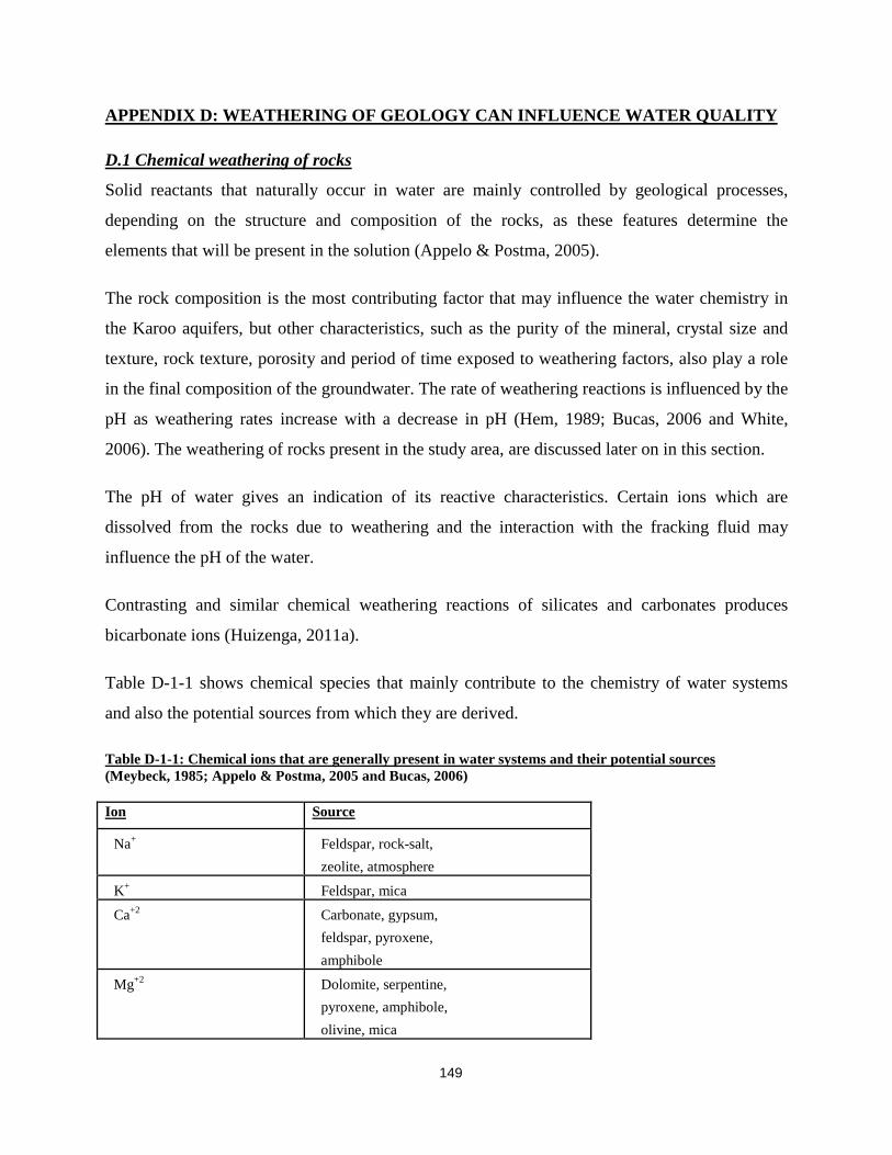
149

APPENDIX D: WEATHERING OF GEOLOGY CAN INFLUENCE WATER QUALITY

D.1 Chemical weathering of rocks

Solid reactants that naturally occur in water are mainly controlled by geological processes,

depending on the structure and composition of the rocks, as these features determine the

elements that will be present in the solution (Appelo & Postma, 2005).

The rock composition is the most contributing factor that may influence the water chemistry in

the Karoo aquifers, but other characteristics, such as the purity of the mineral, crystal size and

texture, rock texture, porosity and period of time exposed to weathering factors, also play a role

in the final composition of the groundwater. The rate of weathering reactions is influenced by the

pH as weathering rates increase with a decrease in pH (Hem, 1989; Bucas, 2006 and White,

2006). The weathering of rocks present in the study area, are discussed later on in this section.

The pH of water gives an indication of its reactive characteristics. Certain ions which are

dissolved from the rocks due to weathering and the interaction with the fracking fluid may

influence the pH of the water.

Contrasting and similar chemical weathering reactions of silicates and carbonates produces

bicarbonate ions (Huizenga, 2011a).

Table D-1-1 shows chemical species that mainly contribute to the chemistry of water systems

and also the potential sources from which they are derived.

Table D-1-1: Chemical ions that are generally present in water systems and their potential sources (Meybeck, 1985; Appelo & Postma, 2005 and Bucas, 2006)

Ion Source

Na+ Feldspar, rock-salt, zeolite, atmosphere

K+ Feldspar, mica

Ca+2 Carbonate, gypsum, feldspar, pyroxene, amphibole

Mg+2 Dolomite, serpentine, pyroxene, amphibole, olivine, mica

150

SiO2 Silicate minerals

PO4 -3 Organic matter, phosphate minerals (apatite)

Cl- Rock salt, atmosphere HCO3

- Carbonate minerals, organic matter

SO4-2

Atmosphere, gypsum, sulphide minerals

NO3-2 Atmosphere, organic matter

D.1.2 Silicate weathering

Incongruent silicate weathering is explained by the following reaction:

Si-mineral + H2O + CO2 = Aluminum-residue + cations + HCO3 - + H4SiO4, where the

Aluminum-residue settles to the bottom of the river and accumulates in the sediment. The main

reason why aluminium stays behind as an insoluble residue is because it is immobile. This

residue is usually one of the clay minerals such as smectite or kaolinite. The type of clay mineral

is however, dependant on the silicate mineral which is exposed to chemical weathering and the

extent of weathering which the rock has undergone (Huizenga, 2011a).

H4SiO4 forms as weathering product from the weathering equation, due to the fact that

precipitation of SiO2 is usually improbable.

Silica is present in mineral phases such as quartz, mica, feldspars, olivine, pyroxene and

amphibole. These are minerals which is present in rocks, applicable in this paper.

Silicate weathering is the only source of silica that is present in nature. Thus, the silica

concentration in natural waters is a good indication of the extent of silica weathering that occurs

(Bucas, 2006).

The chemical weathering of mafic silicates, are more rapid than the chemical weathering of

rocks that have a felsic nature. Silicate weathering is generally a slow process, but it is one of

the main tributaries for dissolved particles in surface water and groundwater systems, as it is

responsible for about 50% of total dissolved solid loads in rivers on Earth (Huizenga, 2011a).

Quartz, a main substance in shale, produces silica as its chemical composition is SiO2, but is not

as susceptible to weathering as other silicate minerals.

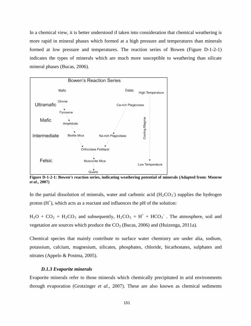
151

In a chemical view, it is better understood if taken into consideration that chemical weathering is

more rapid in mineral phases which formed at a high pressure and temperatures than minerals

formed at low pressure and temperatures. The reaction series of Bowen (Figure D-1-2-1)

indicates the types of minerals which are much more susceptible to weathering than silicate

mineral phases (Bucas, 2006).

Figure D-1-2-1: Bowen’s reaction series, indicating weathering potential of minerals (Adapted from: Monroe et al., 2007)

In the partial dissolution of minerals, water and carbonic acid (H2CO3-) supplies the hydrogen

proton (H+), which acts as a reactant and influences the pH of the solution:

H2O + CO2 = H2CO3 and subsequently, H2CO3 = H+ + HCO3- . The atmosphere, soil and

vegetation are sources which produce the CO2 (Bucas, 2006) and (Huizenga, 2011a).

Chemical species that mainly contribute to surface water chemistry are under alia, sodium,

potassium, calcium, magnesium, silicates, phosphates, chloride, bicarbonates, sulphates and

nitrates (Appelo & Postma, 2005).

D.1.3 Evaporite minerals

Evaporite minerals refer to those minerals which chemically precipitated in arid environments

through evaporation (Grotzinger et al., 2007). These are also known as chemical sediments

152

(McCarthy & Rubidge, 2005). Minerals may precipitate in aquifers due to weathering and

evaporation (Appelo & Postma, 2005).

The weathering of silicate minerals produces secondary clay minerals, which continue to erode

in weathering conditions such as groundwater flow in aquifers. Clay minerals mainly consist of

Al-silicates, combined with other cations. With continual weathering, cations, followed by

silicon go into dissolution until soluble Al-hydroxide remains. With increased temperatures in

arid climate regions, evaporation occurs and causes possible precipitation of suite minerals in the

aquifers. Evaporation concentrates the solution and leads to the precipitation of minerals such as

calcite, gypsum and chloride-salts. The changes in solute concentration and the precipitation

sequence of the minerals during evaporation, can be calculated for a given initial water

composition (Appelo & Postma, 2005).

Ion exchange reactions between cations in solution and those which form part of the mineral

surfaces, can possibly produce major changes in the water chemistry as soon as the composition

of the infiltrating water is different from the water that is present (Appelo & Postma, 2005).

D.1.4 Carbonate weathering

In this study, groundwater is in contact with different rock formations, depending on the position

of the aquifers. Some of the rock formations such as sandstone and mudstone, overlying the

shale, which can possibly interact with groundwater are, may contain carbonate minerals.

Carbonates are highly soluble and saline. Minerals such as calcite (CaCO3) and dolomite

(CaMg(CO3)2) are carbonate minerals.

Carbonate minerals weathers easily and is indicated in the following reactions:

𝐶𝑎𝐶𝑂₃ + 𝐻₂𝑂 + 𝐶𝑂₂ → 𝐶𝑎²⁺ + 2(𝐻𝐶𝑂₃)⁻

(𝐶𝑎𝑀𝑔(𝐶𝑂₃)₂) + 2𝐻₂𝑂 + 2𝐶𝑂₂ → 𝐶𝑎²⁺ + 𝑀𝑔²⁺ + 4(𝐻𝐶𝑂₃)⁻

The weathering products of these minerals are usually Ca2+ and Mg2+, with a bicarbonate

concentration which is equal to the cation concentration (Appelo & Postma, 2005).

153

Carbonate rocks acts as a buffering agent in waters that is affected by acid mine drainage.

This may be of significance as it neutralizes low pH that may be caused by sulphur rich rocks,

solutes in the atmosphere or the fracking fluid. However, increased dissolution of carbonate

rocks causes increased salinity in the water due to higher TDS (Appelo & Postma, 2005).

D.2 Weathering of the geology in the Victoria West region

The weathering process of sedimentary rocks generally produces clay. The composition and

weathering processes which the rocks applicable in this study undergo, is displayed below in

Table D-2-1.

154

Table D-2-1: Rocks and their associated weathering patterns in the Victoria West area of the Karoo (Anon., Undated and Coetzee, 2008)

Rock Mineral and Chemical

composition

Type of

weathering

Weathering equation Products

Sandstone Quartz (SiO2) Silicate,

Carbonate

and

Evaporite

weathering

Quartz Rounded quartz grains Mainly Clays and

associated ions Feldspar (K,Na,Ca)Al(Si,Al)Si2O8

Feldspar Clay (kaolinite, illite or

montmorillonite) with Na, Ca, and K ions

Mica (KAl2(AlSi3)O10(OH)2) and/or K(Mg,Fe)3AlSi3O10(F,OH)2

Mica Clay (kaolinite, illite or montmorillonite)

with Na, Ca, and K ions. Insoluble Fe present for

biotite.

Carbonates (Ca, Mg)CO3 or (Na, K)2CO3

Carbonates Ca, Mg, Na or K with CO ions

Clay minerals (Silicates) Clay Clay and ions (1:1 Clay produces a 2:1

Clay)

Mudstone Quartz (SiO2) Silicate and

Evaporite

weathering


associated ions Mica (KAl2(AlSi3)O10(OH)2)

and/or K(Mg,Fe)3AlSi3O10(F,OH)


with Na, Ca, and K ions. Insoluble iron oxides

155

2 present for biotite.


Clay)

Iron Hydroxides and Iron Oxides Fe(O,OH)6

Iron -Hydroxides and Oxides Iron and

Hydroxide ions

Dolerite Quartz (SiO2) Silicate

weathering


associated ions Amphibole Mg,Fe,Ca,Na)2-3 (Mg,Fe,Al)5(Si,Al)8O22OH2

Amphibole Clay and highly insoluble iron

oxides; Limonite, clay

Plagioclase (Na,Ca)Al(Si,Al)Si2O8

Plagioclase Clay

Shale Quartz (SiO2) Silicate

and

Evaporite

weathering


associated ions Mica (KAl2(AlSi3)O10(OH)2) and/or K(Mg,Fe)3AlSi3O10(F,OH)2


with Na, Ca, and K ions. Insoluble iron oxides

present for biotite.


Clay)

Iron Hydroxides and Iron Oxides Fe(O,OH)6

Iron -Hydroxides and Oxides Iron and

Hydroxide ions

Kimberlite Olivine ((Mg,Fe)2SiO4)

Silicate, Olivine Serpentine, Limonite, Clay Mainly Clays and

156

Phlogopite (KMg3Al(OH)2Si4O10)

Carbonate

and

Evaporite

weathering

Phlogopite Clay associated ions

Ilmenite (FeTiO3) Ilminite Ilminite sands (geology.com)

Perovskite (CaTiO3) Perovskite Anatase

Carbonates (Ca, Mg)CO3 or (Na, K)2CO3

Carbonates Ca, Mg, Na or K with CO ions

Enstatite (Mg2Si2O6)

Enstatite Serpentine, Clay

Cr-Diopside (Ca(Mg,Fe)Si2O6)

Clinopyroxene Clay and highly insoluble iron

oxides

Chlorite (Mg,Fe)3(Al,Si)4O10(OH)2. (Mg, Fe)3(OH)6

Chlorite Clay

157

D.3 Sources of solutes in the atmosphere

H2O, SO2, NH3, N2O, NO2, HCl, CO and CO2 are all gasses which are produced from

anthropogenic activities such as the burning of fossil fuels, metallurgical and industrial

processes, etc. Natural tributaries like biochemical processes in soil and water, and geothermal

activity, may also produce gases. Gases like these in the atmosphere may have an effect on the

chemical properties of rainwater and subsequently, also on the waters of rivers and subsurface

waters (Hem, 1989). They come in contact with water, may form acids and increase weathering

rates. This leads to increased compounds such as sulphates, ammonia, nitrates, carbonates and

chlorides in river water (Hem, 1989).

During precipitation, CO2 in the atmosphere reacts with rain and produces carbonic acid.

H2O + CO2 = H2CO3

This results in acid rain as carbonic acid dissociates to form hydrogen and bicarbonate:

H2CO3 = H+ + HCO3-

The H+ serves as the originator of acidic conditions which causes rocks to weather more rapidly.

This as a whole has an impact on the chemistry of river waters as well as groundwater due to

infiltration and groundwater- surface water interaction (Bucas, 2006).

158

APPENDIX E: MODEL COMPARISON

Model Description of model Capabilities Limitations

MODFLOW Modflow is the industry

standard software for 3D

and 2D groundwater flow

and contaminant

transport modelling.

Unparalleled Power and

Performance

A sufficient amount of

the equation’s

variables must be

known to describe

groundwater-flow

with a partial-

differential equation

Flexible Grid Options It only models porous

flow

It is used for integrated

conceptual and numerical

groundwater modelling.

GIS Integration It cannot model or

simulate fracturing of

the geology

Powerful Data

Visualization

The software is best

for models with

simple geology, basic

properties and

boundary conditions.

The model is based on a

finite-difference method,

which initiate systems of

simultaneous linear

algebraic difference

equations.

Efficiently Manage

Multiple Models

MODFLOW uses

numerical methods to

solve the flow equation

The model applies finite

difference methods to

solve a set of differential

equations across a 3D

grid

Integrated 3D Conceptual

and Numerical

Groundwater Modeling

Flexible Modeling

159

Approaches

This model includes a

complete set of tools

which enables the

modelling and simulation

of water quality,

groundwater supply, and

source water protection

initiatives. The model

includes:

• MODFLOW-

2000, 2005, NWT

• MODGLOW-

LGR

• SEAWAT v.4

• MT3DMS

• MODPATH

• Zone Budget

• PHT3D

• PEST v.12.3

A Complete Groundwater

Modeling System

UTCHEM UTCHEM is a 3D

chemical flooding

simulator

Phase saturations and

concentrations are

resolved in a flash routine

A sufficient amount of

the equation’s

variables must be

160

UTCHEM solves both the

pressure equation and

species conservation

equations

known to describe

groundwater-flow

with a partial-

differential equation

The model applies finite

difference methods to

solve a set of differential

equations across a 3D

grid

Simulates the final

conditions and transport

of NAPLs in the saturated

and unsaturated zones of

an aquifer

UTCHEM input

process is inefficient

and tedious

UTCHEM contains the

equations needed to

estimate phase

partitioning, in relation to

DNAPLs

Several major physical

phenomena are modeled

in the simulator:

• dispersion • diffusion • dilution effects • adsorption for oil, surfactant and polymer • relative permeability • capillary pressure • cation exchange reactions • phase density • compositional phase viscosity • phase behavior (pseudoquaternary) • aqueous reactions • partitioning of chemical species between oil and water • dissolution/precipitation

A 3D finite difference

model for multiphase

flow, transport and

chemical flooding, the

code has also been

modified to a general-

purpose NAPL simulator.

SUTRA A porous 3-D finite-

element/finite-difference

model which simulates

saturated-unsaturated,

SUTRA models saturated

and unsaturated, variable-

density ground-water

flow. It also models solute

Models flow of

different densities

related to differences

in temperatures and

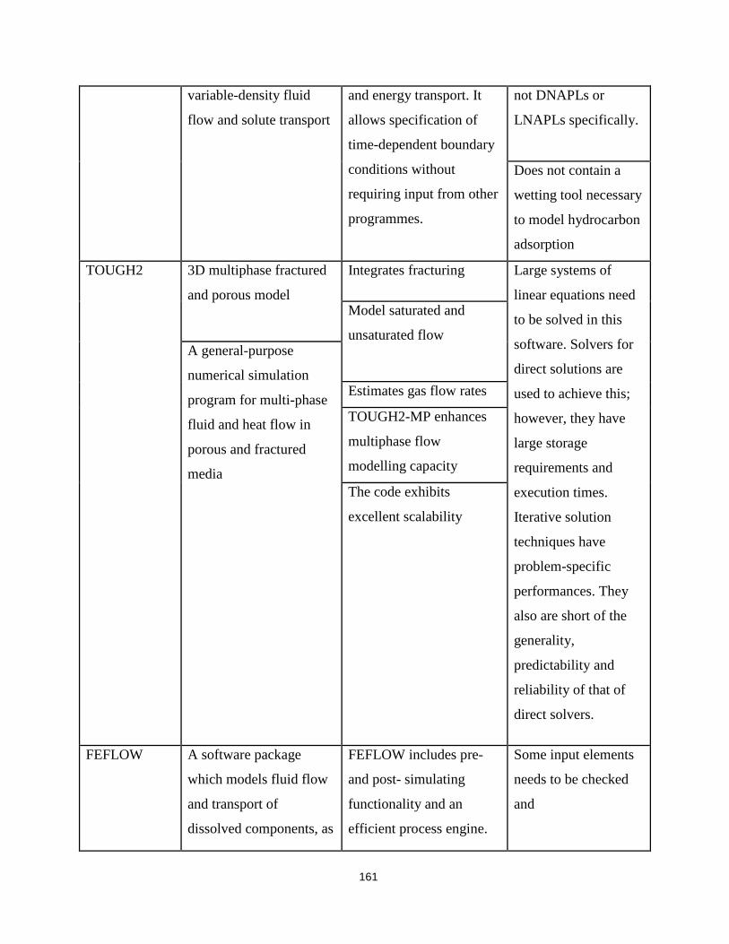
161

variable-density fluid

flow and solute transport

and energy transport. It

allows specification of

time-dependent boundary

conditions without

requiring input from other

programmes.

not DNAPLs or

LNAPLs specifically.

Does not contain a

wetting tool necessary

to model hydrocarbon

adsorption

TOUGH2 3D multiphase fractured

and porous model

Integrates fracturing Large systems of

linear equations need

to be solved in this

software. Solvers for

direct solutions are

used to achieve this;

however, they have

large storage

requirements and

execution times.

Iterative solution

techniques have

problem-specific

performances. They

also are short of the

generality,

predictability and

reliability of that of

direct solvers.

Model saturated and

unsaturated flow A general-purpose

numerical simulation

program for multi-phase

fluid and heat flow in

porous and fractured

media

Estimates gas flow rates

TOUGH2-MP enhances

multiphase flow

modelling capacity

The code exhibits

excellent scalability

FEFLOW A software package

which models fluid flow

and transport of

dissolved components, as

FEFLOW includes pre-

and post- simulating

functionality and an

efficient process engine.

Some input elements

needs to be checked

and

162

well as heat transport

processes in the

subsurface.

A graphical user-friendly

interface ensures

extensive modelling

options.

re-worked

Limitation in terms of

calibration as

FEFLOW does not

have a good way to

check mass

balance.

Software includes a public

programming interface for

user code.

Offers manual steady state

calibration

Automated (PEST)

optimization of

parameters and assesses

confidence bounds

It offers full transient

calibration (future)

MIKE-SHE An advanced integrated

hydrological modelling

system which simulates

water flow in the entire

land based phase of the

Integrates geological data

Integrates interaction

between all major

hydrological

components such as

surface water, soil

163

hydrological cycle

including groundwater

flow.

Links with ArcView and

GIS

water and

groundwater.

Therefore, not

appropriate for this

study as only

groundwater flow and

transport as well as

NAPL flow and

transport will be the

focus.

The model requires a

certain amount of

input

MARS

A finite-element ground

water multiphase

simulation model which

also incorporates

bioremediation. The

model an accurate

version of inconsistent

physical boundaries and

material in

heterogeneous and

anisotropic media.

Models multiphase flow

and transport in the

saturated and unsaturated

zone. The software

package encompass solute

transport models. Models

flow and transport of

species in groundwater

with numerous pumping

and/or injection wells.

Models fractured systems.

Incorporates

bioremediation.

Only the light non-

aqueous phase liquids

(LNAPLs) are

modelled. Dense non-

aqueous phase liquids

(DNAPLs) are not

modelled.

Aqueous phase

transport of limited

chemical species can

be modelled-

therefore, not

adequate as multiple

species are present in

the fracking fluid.

164

(Moridis & Pruess, 1997; Reservoir Engineering Research Program, Texas, 2000; USGS, 2005;

TOUGH2-MP, 2007; FEFLOW, 2012; Schlumberger:Water Services, 2013; USGS, 2013; U.S.

Environmental Protection Agency: Ground Water and Ecosystems Restoration, 2013; MIKE-

SHE, Undated; MARS, Undated)

165

APPENDIX F: RAINFALL AND GROUNDWATER CHEMISTRY DATA USED TO DETERMINE RECHARGE

(DWA, 2013b; South African Weather Service, 2013) Table F-1: Rainfall data for study area

Monthly Daily Rain (mm) Data for station [0141066 3] - RHEBOKSFONTEIN Measured at 08:00 Year JAN FEB MAR APR MAY JUN JUL AUG SEP OCT NOV DEC 1950 14.5 56.3 88.4 96.5 31 0 0 15.1 34.6 21.9 40.1 2.5 1951 5 13 12.7 0 6.1 2.8 3 0 7.1 0 0 0 1952 1.3 37.8 12.6 7.3 4.5 0.3 16.7 2.1 8 1.2 6.8 6.7 1953 0 56.4 18 16.4 8.8 2.2 7.1 8.2 0 36.6 45 21.8 1954 7.5 5.3 105.3 59.7 8.3 7.5 0 1 0 0 29.2 12.4 1955 17.2 31.2 0 47.8 3.4 17.6 12.3 10.2 1.7 2.9 34.5 40 1956 21.7 50.1 88.3 23.3 19.8 5.4 4.4 1.6 0.7 16.3 47 50.4 1957 1.2 27.6 53.9 0 2.5 18.7 8.3 0 8.5 14.1 1.6 32.9 1958 41.7 5.2 1.3 10.5 60.6 1.6 0 0 12.8 4 25.1 28.6 1959 15.2 27.1 44 11.3 14.2 0.2 7.6 0 0 6.2 3.5 18 1960 11.3 22.4 38 16.1 24.6 13 17.4 46.1 5 0 32.8 11.5 1961 37.8 0 164 81.5 14 35.7 26 0 8 0 15.4 2 1962 12 17.5 0 7.3 0 5.7 2.2 0 0 0 13 0 1963 114.8 9.3 56 56 7.4 14 14.7 10.8 3.5 57.3 38.1 26.5 1964 0.3 9 17.4 18 0 10.4 0 10.8 15.4 33.2 13.2 20.9 1965 12.1 10.8 41.3 49 0 1 17.7 5.5 3 21.6 35.5 0 1966 92.5 6.5 0 6 0 12.4 0 0 16.7 8 0 11 1967 39.5 56.5 56.5 84 27 8 3.5 14 0 16 14.9 0.5 1968 0 0 87.5 16 29.2 2.2 0 1.5 10.7 16 7 2.3 1969 0 73 21.2 72.2 39.5 3.2 4 0 0 8 10 0 1970 7.5 20.3 0 16.3 34 10.5 0 86 0 13 1.5 16.5 1971 31.7 51.5 4.5 18.5 18 30 26.5 24.5 0 29.5 0 6.5

166

1972 46 23 59.2 61.5 3.5 1 2 0 8.5 22.3 0 0 1973 0 38.5 108 55 5 0 35 6 0 11.5 9 70 1974 68 248 89.5 35.5 11.5 0 0 29.5 0 0 27.5 11.2 1975 61 70.5 96.5 24 12 21 21 0 0 2.5 61.5 89 1976 89.5 111.7 123 36 38.5 1 7.5 1.5 11.5 58.5 6.5 26.7 1977 16 16.2 69 71.1 32.7 0 0 0 14.5 17 65 53.1 1978 16.5 20 23 29.5 0 0 3 14 5.5 9 0 16.1 1979 22.5 84.5 1 3 21 7.2 11.5 7.5 0 38 9 0 1980 14.5 4.5 63.7 0 1.5 5 0 38.5 16.5 0 32.5 18.5 1981 18 58 42.5 0 41 2.5 16 49.5 2 42.5 21.9 40 1982 0 11 4 41.5 0 2 26.5 4.5 0 38.5 5 11.5 1983 3.5 0 21.5 37.5 8.5 37.5 18 0 27 0 43.2 23 1984 0 0 9.5 40.5 2.5 0 0 10 0 13 37 0 1985 61 16.5 6.5 14 0 4.5 0 0 0 46.5 50 96 1986 48.5 20 21.5 83 0 14.5 0 0 1.5 24.5 14.5 4 1987 0 37 20.5 36 24 3 0 0 47.5 4 77.9 18.5 1988 5.5 125 69.5 34 5.5 8 0 7.5 32.5 15 8 49 1989 16 165.5 7.5 33.5 17 0 7.5 0 0 7.5 23.5 0 1990 0 48 11.5 53 0 46 10 0 0 0 1.5 0 1991 27 0 32.5 15 0 23 0 0 41 62.5 15 0 1992 0 4.5 26.5 3.5 0 0 5 14 0 22 2.5 0 1993 0 39 0 0 2.3 24 0 0 0.4 0 34.5 24.5 1994 56 81.5 51.5 0 0 0 7 0 0 0 11 0 1995 33 15.5 71.5 5.5 62.5 0 0 20 12.5 0 93 85 1996 53.5 54.7 20 16 0 0 24 12.5 0 0 40.8 37 1997 38.5 0 76 18 5.5 18.5 1.6 0 0 0 0 0 1998 46.5 0 85 6 8.5 0 0 0 0 0 0 31 1999 23 0 0 0 0 0 0 0 0 0 26 82.5 2000 0 5 92.5 47 0 0 0 0 6 2 10.5 9.5 2001 0 27 41.5 35 2 5 23 0 61 2.5 49.5 20

167

2002 48.5 21 49 0 22 23.5 0 26 5 2.5 0 75.5 2003 0 0 118.5 4.5 17 0 0 0 0 0 7 0 2004 46 44 24.5 56 0 2.4 0 0.1 17 15 16 0 2005 30 39 15 9.5 49 11.5 0 0 0 26 21 15 2006 68 39.5 27 41.5 23 0 0 62 5 0 0 25.5 2007 24 15 20 19 1.5 9.5 9 0 19 31.5 24.5 62.5 2008 56 42 25 17 15 45 0 0 0 0 0 0 2009 0 87.5 103.3 48 0 26 8.5 0 0 44 26 18 2010 48 55 41 15.5 0 0 0 0 0 0 36.3 64 2011 36.5 140 61 6 10.5 0 3.2 0 0 0 0 0 2012 25 75 53.5 61.5 0 9 17 0 0 75.5 43 74.5 2013 16.5 0 132.5 Average 25.73906 38.59219 45.7125 28.99683 12.63333 8.777778 6.788889 8.579365 7.453968 14.91429 21.65556 23.20794 Monthly Daily Rain (mm) Data for station [0141075 9] - DRIEFONTEIN Measured at 08:00 Year JAN FEB MAR APR MAY JUN JUL AUG SEP OCT NOV DEC 1950 9.7 45 64.7 77.6 30.3 2 0.5 14.1 43.7 6.4 34.8 13.2 1951 18.4 31 23.4 5.3 18.8 4 1 0 15 2 0 0 1952 1.5 66.7 26.2 20.9 10.7 10.2 39.4 6.1 11.4 10.2 10.2 18.1 1953 10.4 Average 10 47.56667 38.1 34.6 19.93333 5.4 13.63333 6.733333 23.36667 6.2 15 10.43333 Monthly Daily Rain (mm) Data for station [0141204 2] - VICTORIA WEST - TNK Measured at 08:00 Year JAN FEB MAR APR MAY JUN JUL AUG SEP OCT NOV DEC 1967 0 1.3 4.7 0 11.2 31.5 2.2 1968 0 0 41.1 11.5 32.5 1.6 0 0 19 16.5 7.5 0.4 1969 0 78.5 17.3 60.5 36.2 0.2 0 0 0 24.5 5.5 8

168

1970 28 19 0 15.5 36.8 10.7 0 26 0 8 6.5 12.5 1971 33 74.5 12.5 30.9 19.5 20.5 30 9 0 13.5 0 21 1972 55.5 35 90 34 0 0 1 0 4 16.5 0 0 1973 0 55.5 133 47 10.5 0 40 0 0 11.5 20.5 114 1974 69 170.5 87.5 30.5 6.2 0 0 43 0 0 34 14.5 1975 34.2 61.5 115.5 44 9 31.5 7 0 9.5 0 24.9 47.8 1976 138.4 76.7 114.5 29.9 26.5 0 8.7 1.5 4 51.5 2 36.6 1977 10.5 55.3 49.8 75 30.5 1 0 0 12.5 17.5 0 90.5 1978 18.8 18.2 30.6 29.5 2.5 0 0 9.5 0.5 2 1.5 31.4 1979 10.5 63.5 2.5 10 16 4 1.3 25.5 3 43.5 30.5 1.3 1980 0 30.5 67.9 8.5 0 0.6 0 32.4 16.5 0 46.6 24.8 1981 37.5 76.5 61.2 0 33.5 2.5 0 55.2 0.5 55 6.2 30 1982 0 16 20.5 44.1 0 0 22.8 4.5 6 29 5.5 10.2 1983 4 0 20 22 16 34 21 0 20.5 0 59.2 26.4 1984 2.5 0 8.5 22 10.5 8 0 0 0 17.1 46 0 1985 53 20.1 7 9 0 6.8 0 0 0 31.2 52.4 148.6 1986 58.9 9.7 24.1 45.6 0 14.2 0.4 0.3 0 16.8 6.3 0 1987 0 11.5 27.5 31.6 23.5 3.6 0.5 0.1 33.4 9.6 35 21 1988 6.5 234.5 128.3 56.5 10.1 10.9 6 4 32 7 8.9 79.8 1989 60.9 72.5 29.7 44.1 13.5 3.5 6.6 0.6 1.3 12.5 43.5 16.7 1990 18.2 33.6 21.2 52.2 3.3 21.7 4.6 0.3 0 2.6 9 32.9 1991 33.9 11.9 91.8 14.2 0 30.5 5.9 0 33.3 43.4 6.5 10.5 1992 0 26 41.7 4.5 0 5.5 8 24.4 0 14.7 14 0 1993 3 29 34.1 47.4 18 28.5 0 4 0.4 18 36.3 18.1 1994 33.9 38.5 79.5 7.2 0 0 3 1 0.8 0 9 0 1995 42.5 18.5 75 1 55.5 0 0 8.5 21.5 4 63.5 78.6 1996 82.5 44.5 25 10.5 6 0 20 16 5.5 19 89.5 3.5 1997 11.5 2 83 10 31 13.5 8.5 0 0 5.3 0 12 1998 16.5 23.9 62.6 8 10 0 0 0 1.7 14.5 3 20 1999 52 3 9.3 4.5 19 0 5.6 0 0 0 5 38.5

169

2000 55.7 33.5 131.3 21 0 4 1 5 38 2.4 23.5 12.5 2001 0 34 63.5 61 3.5 0 20.3 0 46.6 0 49.9 30.3 2002 33.5 25 50.5 18 14.8 10.6 0 39.5 0 0.6 0 69.4 2003 0.4 21 72 15 15 0 0 0 0 37 11 0 2004 96 31.1 33.7 81 0 0 0 0 7 11.5 9.3 7 2005 57 51.5 28 13.5 41 3 0 0.5 0 0.5 17.9 0 2006 115 49.8 33 64 50.5 0 13 45 3 9.5 3.3 33.5 2007 46 60 8 20.1 0.2 7.4 5 0 1.5 78.5 37.5 67.5 2008 56.2 75.8 29.5 12.5 47 53 4 11 0 5 42 0 2009 6 68.4 0 40.5 1.5 17 0 3 0 9 10 15.5 2010 108.3 157.7 68.5 35.5 0.3 4.2 2 0 0 1.5 40 42.5 2011 88.5 168.7 49.6 15.5 38.7 21.3 2.8 0 0 20 12.5 33 2012 38 132.2 58 28 0 9.3 18.6 3.3 4 82 20.5 77 2013 20 1 70 Average 35.56087 50.43696 50.16957 28.59556 15.30222 8.328261 5.845652 8.213043 7.086957 16.81304 21.46087 29.13043 Monthly Daily Rain (mm) Data for station [0141264 6] - VICTORIA WEST - AER Measured at 08:00 Year JAN FEB MAR APR MAY JUN JUL AUG SEP OCT NOV DEC 1950 83.6 31.9 1.3 1.3 13.2 54.8 6.6 36.7 31 1951 33.6 11.5 3.1 19.4 1.3 0.3 3.6 6.2 1952 0.6 119.1 45.3 12.7 14 7.4 1954 40.1 1955 30.2 16.5 39.7 1956 3 1957 18.5 23.1 1959 31.4 22.3 29.3 11.6 13.2 0 1.3 0 11.9 5.2 27.8 1960 1.6 3.2 52.8 14 11.5 3.8 8 20.4 1.3 1 7.1 4.4 1961 31.3 3.2 177.8 72.4 19.2 17.8 40.2 2.1 6.8 0 56.7 9.8

170

1962 17.9 34 29 4 0 7.7 0.9 1.4 1 0 33.9 6.2 1963 102.2 11.8 103 56.2 16.6 22.1 13.1 6.1 6.5 82.4 63.4 26 1964 0 19 26.5 8.2 0 2.8 0 7.5 19 35.7 17.1 58.3 1965 14.5 21.6 29.8 50.6 0 0.8 16 0.3 3.2 31.3 13.7 0.4 1966 73.7 0 2.2 2.8 0 4.6 0 0 14.6 3.4 7.5 2.5 Average 30.34 26.78 50.72 29.01818 12.025 7.754545 9.166667 5.26 11.46 17.49091 27.275 18.48889 Monthly Daily Rain (mm) Data for station [0141498 1] - SLAGBERG Measured at 08:00 Year JAN FEB MAR APR MAY JUN JUL AUG SEP OCT NOV DEC 1950 0 29.5 48.8 97.6 24.6 0.5 0.3 18.2 44.1 3.1 22.9 16.6 1951 10.5 27.1 33 0 8.9 0 1.3 0 5.8 1952 49.3 0 10.4 21.6 4.6 7.1 1953 2.5 78.9 30.4 11 0 3.8 0 0 0 7 55.5 0 1954 0 52.5 147.9 56.5 7.5 0 0 0 0 0 44.5 0 1955 22.8 21.3 6 79 0 23.5 5 0 0 0 34.4 21.3 1956 15.8 63.9 67.8 0 0 0 0 0 0 0 65 38.5 1957 0 30.5 35.2 0 3 24.4 2.3 0 0 7.5 0 0 1958 45.5 0 5.5 5.8 77.7 0 0 0 32 3 0 10.4 1959 11.3 18.5 10.5 7.5 17.3 0 7.3 0 6.5 7 11.8 1960 10.9 6 Average 11.93 32.82 42.78889 28.6 15.44444 5.8 6.55 1.82 10.25556 5.411111 25.98889 11.74444 Monthly Daily Rain (mm) Data for station [0141664 9] - DOMBIETERSFONTEIN Measured at 08:00 Year JAN FEB MAR APR MAY JUN JUL AUG SEP OCT NOV DEC 1950 25.9 35.2 45.2 125.6 33.4 3.6 0.8 15.5 59.5 26.2 59 4.3 1951 12.4 19.3 27.4 2 12.2 4.6 1.8 0 13.7 2.5 0 0 1952 23.7 48.9 41.9 20.1 16 4.3 27.5 4.1 11.6 9.6 14.5 17

171

1953 9.2 64.8 16.4 20.4 0.3 9.8 6.5 5 4 31.4 46.5 48.9 1954 8.1 4 140.8 52.7 18.5 2.5 5 0 0 0 23.5 11 1955 24.7 30.5 15.9 50 10 43 10 1.1 0.9 13 40.4 39.8 1956 33.8 45.7 120.5 9.5 32.7 2.2 8.6 0.3 7.5 24.1 39.3 38.7 1957 25.2 48.2 61 2.3 5.5 23.1 0 3.5 6.9 28 5.8 32 1958 53.3 4.8 11.8 5.9 81.2 0.9 0 0.9 15.5 7.3 18 46.6 1959 15 28.3 53.4 16.1 32.9 0 5.3 1.3 0 3 18 11.6 1960 9.4 18.2 29.4 30.1 27.2 0 6.5 28.4 2.6 6.7 11.5 11.5 1961 18.4 0 231.9 57.7 24.3 31.1 24 5.5 5 0 29.3 17 1962 17 32.2 1 6.2 0 6.9 1.5 5.2 0.2 0.3 20.7 3.5 1963 117.6 7.7 85.8 29.4 0.8 9 10.8 12.5 1.8 42 52.8 29 1964 0 9.5 23.7 19.9 0 16 0 14.5 13.2 26.5 38.9 67 1965 10 7.5 37 60 0 4 21.5 3 0.2 29.2 25.4 5.7 1966 64.5 0.5 13.3 9 0 6.5 0 0 6.3 11.5 7 9.3 1967 76 30 49.5 64.2 19.7 12.4 3.5 8.5 0 13.5 25 2.3 1968 0.7 0 73.5 53.5 22.8 4.2 0 1 8.6 6.5 8.2 3.5 1969 0.5 58.8 8.5 79 30.5 2.2 4.5 0 0 12.8 4 0 1970 4.4 58.1 0 21.3 28.3 8.3 6.2 38.6 0 8 2.5 7.7 1971 30.5 47.7 5.5 31 24 14.3 16 13.2 0 45.5 0.5 0 1972 48.9 8.2 77.5 22.9 3.6 1.1 1.1 0 0 14.4 3.5 0 1973 0 22.8 103.5 35.4 11 0 13.3 23.3 0 5.9 5.7 62.3 1974 41.8 155.4 153.2 43.2 27.6 0 0 32.3 0 0 54.5 4 1975 27.7 50.3 121.4 24.2 9.3 25.3 11.5 0 7.8 0 35.9 90 1976 79.6 84 132.2 30.3 24 0.3 4.6 0 8.3 69.6 10 8 1977 39.5 26.5 47.2 68.2 51.5 0.6 0 0 0 9.2 35.4 55.3 1978 25.3 11.9 32.6 13.4 0 2.3 8.1 12.5 9.7 11.7 0 36.7 1979 0 37.4 7.5 2.5 15.4 0 17.5 1.6 0 34.1 23.3 0 1980 7.4 36.9 44.9 8.2 0 4.2 0 45.7 21.1 13.4 10.8 11.5 1981 45 27.3 52.9 15.5 41.9 1.7 0 47 0 35.1 5.1 35.7 1982 0 12.7 4.5 41.8 0 3.5 28 4 8 27 14.5 21

172

1983 22.8 0 24 14 21.8 29.5 14.6 0 31.2 0 44.8 32.3 1984 0 1 13.5 32.5 17 0 0 4 0 16.7 35.5 0 1985 38.5 33 1.5 11 4.5 9 0 0 4 27.3 56.3 135 1986 73.7 0 40.2 51.1 0 9 0 8.5 7.5 16.5 18.5 0 1987 0 18 6 8 23.5 2 6 0 51 27.5 57 33 1988 27 147.5 26.5 63.5 70.5 0 17.5 6 41.5 24 9 47.5 1989 21 96 32 55 14 0 14 7 7.5 8.5 23 0 1990 5.5 19 10 40 0 46 0 0 0 0 0 24.5 1991 48.5 11.5 42.5 0 0 48.5 0 0 36.5 88 9.5 14.5 1992 0 0 70 0 0 15 5.5 45.5 0 17 0 0 1993 11 59 36 27 17 18.5 0 5 0 11 16.5 34 1994 43 78.5 81.5 8 0 1 1 0 0 0 3 11 1995 33 22.2 84 5 75.5 0 0 17.5 6.5 9.5 66.5 101.5 1996 50 51.5 1.5 0 0 0 24 12.5 0 21 92.5 53 1997 42 13.5 72 0 34.5 20 5.5 0 0 0 0 5.5 1998 38.5 7 125 22.5 4.5 0 6.5 0 7.5 4 0 13 1999 32 0 10.5 6 21 0 10.5 0 0 0 17 103 2000 47.5 60.5 68 50 0 2 0 0 47.5 2 14.5 4 2001 10 18.5 46 75.5 0 8 19.5 0 70 4.5 30.5 46.5 2002 8 19 31 3 21 32.5 2.5 17.5 6 83 7 65 2003 0 15 115.5 21.5 21.5 0 0 5 12.5 13.5 49.5 0 2004 67 36.5 53.5 115.5 0 2.5 3.5 0 24.5 13.5 8 29.5 2005 43.5 22.5 4 31 26.5 7 0 1 0 18 68.5 0 2006 166.5 61.5 56.5 53.5 52.5 0 8 121.5 0 18.5 4.5 79.5 2007 39.5 15 17 82 1 11.5 0 0 0 123.5 51 70.5 2008 120.5 72.5 24.5 10 29.5 56 0 7 0 1 10 11 2009 17 179 25 55.5 13 42.5 9.5 0 0 68 23.5 12.5 2010 144 160.5 53.5 20 0 2 0 0 0 4 19 90 2011 109.5 124.5 101 37 56 18.5 8 2 0 13 0 48 2012 27 109 97 97 1.5 21.5 34 0.5 2.5 91 27 227

173

2013 28.5 0 190 Average 34.53906 39.45313 53.59375 32.80317 17.95079 10.32381 6.892063 9.349206 9.025397 20.51587 23.04127 32.09841

Table F-2: Calculated Monthly and Annual Average Precipitations

Monthly Daily Rain (mm) Data for station [0141066 3] - RHEBOKSFONTEIN Measured at 08:00 Annual Precipitation

Year (1950-2013) JAN FEB MAR APR MAY JUN JUL AUG SEP OCT NOV DEC

Average 25.73906 38.59219 45.7125 28.99683 12.63333 8.777778 6.788889 8.579365 7.453968 14.91429 21.65556 23.20794 243.0516865

Monthly Daily Rain (mm) Data for station [0141075 9] - DRIEFONTEIN Measured at 08:00


Average 10 47.56667 38.1 34.6 19.93333 5.4 13.63333 6.733333 23.36667 6.2 15 10.43333 230.9666667

Monthly Daily Rain (mm) Data for station [0141204 2] - VICTORIA WEST - TNK Measured at 08:00


Average 35.56087 50.43696 50.16957 28.59556 15.30222 8.328261 5.845652 8.213043 7.086957 16.81304 21.46087 29.13043 276.94343

Monthly Daily Rain (mm) Data for station [0141264 6] - VICTORIA WEST - AER Measured at 08:00


Average 30.34 26.78 50.72 29.01818 12.025 7.754545 9.166667 5.26 11.46 17.49091 27.275 18.48889 245.7791919

Monthly Daily Rain (mm) Data for station [0141498 1] - SLAGBERG Measured at 08:00


Average 11.93 32.82 42.78889 28.6 15.44444 5.8 6.55 1.82 10.25556 5.411111 25.98889 11.74444 199.1533333

174

Monthly Daily Rain (mm) Data for station [0141664 9] - DOMBIETERSFONTEIN Measured at 08:00


Average 34.53906 39.45313 53.59375 32.80317 17.95079 10.32381 6.892063 9.349206 9.025397 20.51587 23.04127 32.09841 289.5859375 Average Annual Precipitation 247.580041

Table F-3: Selected calibrated recharge values which form part of model recharge

m/day mm/a Percentage Recharge of Precipitation (%)

9.74E-06 3.55364 1.43535 0.000044 16.06 6.486791 0.00004 14.6 5.897083 0.000036 13.14 5.307375 3.39E-05 12.3808 5.000726 0.00003 10.95 4.422812 0.000026 9.49 3.833104 0.000022 8.03 3.243396 0.000018 6.57 2.653687 0.000014 5.11 2.063979 0.00001 3.65 1.474271 9.79E-06 3.57335 1.443311 9.7E-06 3.5405 1.430043 0.000008 2.92 1.179417 4.85E-06 1.77025 0.715021 4.33E-06 1.578625 0.637622 3.8E-06 1.387 0.560223 3.39E-06 1.23808 0.500073 1.7E-06 0.6205 0.250626

Calculated recharge value by means of chloride method

175

1.7E-06 0.61904 0.250036 0.000001 0.365 0.147427 5E-07 0.1825 0.073714

176

Table F-4: Chloride concentrations measured at different monitoring stations on boreholes in quaternary catchment D61E with Harmonic Mean

Monitoring Point ID

Monitoring Point Name Latitude Longitude Cl- concentration (mg/L)

182215 3123AC00203 VICTORIA WEST ALLOTMENT -31.4378 23.12611 16.96 182215 3123AC00203 VICTORIA WEST ALLOTMENT -31.4378 23.12611 16.7 182215 3123AC00203 VICTORIA WEST ALLOTMENT -31.4378 23.12611 16.579 182215 3123AC00203 VICTORIA WEST ALLOTMENT -31.4378 23.12611 16.556 182217 3123AC00208 RUIGTE FONTEIN -31.3892 23.036389 1343.051 182217 3123AC00208 RUIGTE FONTEIN -31.3892 23.036389 74.601 182217 3123AC00208 RUIGTE FONTEIN -31.3892 23.036389 73.949 182217 3123AC00208 RUIGTE FONTEIN -31.3892 23.036389 73.292 182217 3123AC00208 RUIGTE FONTEIN -31.3892 23.036389 70.733 182669 3123AC00209 VICTORIA WEST ALLOTMENT -31.4483 23.12605 50.207 182669 3123AC00209 VICTORIA WEST ALLOTMENT -31.4483 23.12605 49.152 182669 3123AC00209 VICTORIA WEST ALLOTMENT -31.4483 23.12605 47.64 182671 3123AC00215 VICTORIA WEST ALLOTMENT -31.4483 23.12635 56.029 182671 3123AC00215 VICTORIA WEST ALLOTMENT -31.4483 23.12635 53.541 182673 3123AC00223 VICTORIA WEST ALLOTMENT -31.4483 23.12634 52.535 182673 3123AC00223 VICTORIA WEST ALLOTMENT -31.4483 23.12634 52.282 182673 3123AC00223 VICTORIA WEST ALLOTMENT -31.4483 23.12634 51.786 182675 3123AC00224 VICTORIA WEST ALLOTMENT -31.4394 23.13502 42.819 182677 3123AC00225 VICTORIA WEST ALLOTMENT -31.4464 23.09704 157.278 182677 3123AC00225 VICTORIA WEST ALLOTMENT -31.4464 23.09704 155.681 182677 3123AC00225 VICTORIA WEST ALLOTMENT -31.4464 23.09704 137.366 182659 3123AC00227 VICTORIA WEST ALLOTMENT -31.445 23.09971 139.256 182659 3123AC00227 VICTORIA WEST ALLOTMENT -31.445 23.09971 131.221 182654 3123AC00229 RUIGTEFONTEIN -31.4128 23.0458 28.859 182654 3123AC00229 RUIGTEFONTEIN -31.4128 23.0458 27.126 150476 AMSTERDAM (DUP NAME 10919) -31.3417 23.078333 42.1

177

150532 ANNEXGROOTBOONTJIES -31.2883 23.171667 710 164622 BIEDJESFONTEIN (DUP NAME 23017) -31.5042 23.15 277.9 164623 BIEDJESFONTEIN (DUP NAME 23018) -31.5244 23.15 43.5 164624 BIEDJESFONTEIN (DUP NAME 23019) -31.5264 23.170278 156.3 164626 BIEDJESFONTEIN (DUP NAME 23021) -31.47 23.145278 46.6 164627 BIEDJESFONTEIN (DUP NAME 23022) -31.4819 23.134444 78.6 164628 BIEDJESFONTEIN (DUP NAME 23023) -31.5081 23.1 39.2 164629 BIEDJESFONTEIN (DUP NAME 23024) -31.5328 23.112778 97.8 164631 BIEDJESFONTEIN (DUP NAME 23026) -31.5 23.139167 96.8 164632 BIEDJESFONTEIN (DUP NAME 23027) -31.4994 23.14 137.7 164633 BIEDJESFONTEIN (DUP NAME 23028) -31.5019 23.1425 98.7 164634 BIEDJESFONTEIN (DUP NAME 23029) -31.4867 23.194444 71.4 164625 BIEDJESFONTIEN (DUP NAME 23020) -31.5531 23.158056 115.2 164630 BIEDJESFONTIEN (DUP NAME 23025) -31.5011 23.126944 161.2 146970 BIEJESFONTEIN (DUP NAME 8237) -31.5528 23.156667 92.6 146971 BIEJESFONTEIN (DUP NAME 8238) -31.5028 23.141944 124.8 164122 BIESIESFONTEIN (DUP NAME 22611) -31.4925 23.188889 389.6 164122 BIESIESFONTEIN (DUP NAME 22611) -31.4925 23.188889 291.7 165024 BIESIESFONTEIN (DUP NAME 23321) -31.4719 23.1725 72 165024 BIESIESFONTEIN (DUP NAME 23321) -31.4719 23.1725 69 165024 BIESIESFONTEIN (DUP NAME 23321) -31.4719 23.1725 67.6 165024 BIESIESFONTEIN (DUP NAME 23321) -31.4719 23.1725 66.7 165024 BIESIESFONTEIN (DUP NAME 23321) -31.4719 23.1725 63.8 165024 BIESIESFONTEIN (DUP NAME 23321) -31.4719 23.1725 63.2 165024 BIESIESFONTEIN (DUP NAME 23321) -31.4719 23.1725 63.2 165024 BIESIESFONTEIN (DUP NAME 23321) -31.4719 23.1725 62.6 165024 BIESIESFONTEIN (DUP NAME 23321) -31.4719 23.1725 61.1 165024 BIESIESFONTEIN (DUP NAME 23321) -31.4719 23.1725 61.1 165024 BIESIESFONTEIN (DUP NAME 23321) -31.4719 23.1725 53.5 165024 BIESIESFONTEIN (DUP NAME 23321) -31.4719 23.1725 52.8

178

174154 BIESJES FONTEIN -31.4914 23.188056 308.2 150488 BIESJESFONTEIN (DUP NAME 10930) -31.49 23.206667 45.6 150490 BIESJESFONTEIN (DUP NAME 10932) -31.4667 23.195 250.9 150491 BIESJESFONTEIN (DUP NAME 10933) -31.4417 23.22 181.5 150492 BIESJESFONTEIN (DUP NAME 10934) -31.4433 23.206667 509.1 150493 BIESJESFONTEIN (DUP NAME 10935) -31.4683 23.18 66.3 150494 BIESJESFONTEIN (DUP NAME 10936) -31.47 23.146667 54.2 151103 BIESJESFONTEIN (DUP NAME 11507) -31.5367 23.238333 65.5 151104 BIESJESFONTEIN (DUP NAME 11508) -31.5067 23.245 48.5 151106 BIESJESFONTEIN (DUP NAME 11510) -31.5033 23.15 175 151107 BIESJESFONTEIN (DUP NAME 11511) -31.525 23.17 386 151107 BIESJESFONTEIN (DUP NAME 11511) -31.525 23.17 384 151108 BIESJESFONTEIN (DUP NAME 11512) -31.525 23.15 38 151110 BIESJESFONTEIN (DUP NAME 11514) -31.5083 23.13 239.4 164180 BIESJESFONTEIN (DUP NAME 22653) -31.4961 23.186667 298.1 164180 BIESJESFONTEIN (DUP NAME 22653) -31.4961 23.186667 265 164181 BIESJESFONTEIN (DUP NAME 22654) -31.4289 23.1925 343.7 164181 BIESJESFONTEIN (DUP NAME 22654) -31.4289 23.1925 318.5 164181 BIESJESFONTEIN (DUP NAME 22654) -31.4289 23.1925 266.3 164181 BIESJESFONTEIN (DUP NAME 22654) -31.4289 23.1925 262.4 164181 BIESJESFONTEIN (DUP NAME 22654) -31.4289 23.1925 262.3 164181 BIESJESFONTEIN (DUP NAME 22654) -31.4289 23.1925 259.6 164181 BIESJESFONTEIN (DUP NAME 22654) -31.4289 23.1925 259.4 164181 BIESJESFONTEIN (DUP NAME 22654) -31.4289 23.1925 249.5 164181 BIESJESFONTEIN (DUP NAME 22654) -31.4289 23.1925 248 164182 BIESJESFONTEIN (DUP NAME 22655) -31.4708 23.192778 399.5 164182 BIESJESFONTEIN (DUP NAME 22655) -31.4708 23.192778 328 164183 BIESJESFONTEIN (DUP NAME 22656) -31.4292 23.192778 497.3 164183 BIESJESFONTEIN (DUP NAME 22656) -31.4292 23.192778 326.8 164183 BIESJESFONTEIN (DUP NAME 22656) -31.4292 23.192778 326.7

179

164187 BIESJESFONTEIN (DUP NAME 22660) -31.4956 23.186667 354 164187 BIESJESFONTEIN (DUP NAME 22660) -31.4956 23.186667 299.8 164188 BIESJESFONTEIN (DUP NAME 22661) -31.4803 23.191111 343.6 164188 BIESJESFONTEIN (DUP NAME 22661) -31.4803 23.191111 329.8 164189 BIESJESFONTEIN (DUP NAME 22662) -31.4333 23.194444 329.6 164613 BIESJESFONTEIN (DUP NAME 23008) -31.5028 23.188611 227.7 164614 BIESJESFONTEIN (DUP NAME 23009) -31.4883 23.189722 84.4 164615 BIESJESFONTEIN (DUP NAME 23010) -31.4119 23.194722 112.7 164616 BIESJESFONTEIN (DUP NAME 23011) -31.4803 23.248611 62.3 164617 BIESJESFONTEIN (DUP NAME 23012) -31.5189 23.261944 56.1 164618 BIESJESFONTEIN (DUP NAME 23013) -31.4847 23.226111 62.4 164619 BIESJESFONTEIN (DUP NAME 23014) -31.5364 23.238333 69.7 164620 BIESJESFONTEIN (DUP NAME 23015) -31.5253 23.188889 249.4 164621 BIESJESFONTEIN (DUP NAME 23016) -31.4994 23.185556 1105.6 165029 BIESJESFONTEIN (DUP NAME 23326) -31.4883 23.19 83 146960 BIESJESFONTEIN (DUP NAME 8227) -31.4244 23.1925 153.9 146961 BIESJESFONTEIN (DUP NAME 8228) -31.4297 23.191944 396 146962 BIESJESFONTEIN (DUP NAME 8229) -31.4461 23.2075 554 146963 BIESJESFONTEIN (DUP NAME 8230) -31.5192 23.261944 35.3 146964 BIESJESFONTEIN (DUP NAME 8231) -31.4689 23.175278 50.1 146965 BIESJESFONTEIN (DUP NAME 8232) -31.4703 23.193611 606.8 146966 BIESJESFONTEIN (DUP NAME 8233) -31.4881 23.190556 71.6 146967 BIESJESFONTEIN (DUP NAME 8234) -31.5225 23.223056 112.8 146968 BIESJESFONTEIN (DUP NAME 8235) -31.4814 23.195 63.4 146969 BIESJESFONTEIN (DUP NAME 8236) -31.4875 23.184722 154.2 146972 BIESJESFONTEIN (DUP NAME 8239) -31.4719 23.174722 58.6 146973 BIESJESFONTEIN (DUP NAME 8240) -31.4894 23.183056 258.3 171875 BIESJESFONTEIN/HOTCHINSON -31.4911 23.1875 264.2 164121 BIESTEFONTEIN -31.4917 23.188889 368.2 164121 BIESTEFONTEIN -31.4917 23.188889 319.3

180

164121 BIESTEFONTEIN -31.4917 23.188889 123.7 148691 BRAKPOORT (DUP NAME 9441) -31.35 23.266667 168 148691 BRAKPOORT (DUP NAME 9441) -31.35 23.266667 102 150486 DRIEHOEK (DUP NAME 10929) -31.42 23.063333 187.6 146977 EED VOGEL FONTEIN -31.5631 23.175 204.5 147191 EEND VOGEL FONTEIN (DUP NAME 8404) -31.5589 23.240833 126.5 147192 EEND VOGEL FONTEIN (DUP NAME 8405) -31.6125 23.151667 66.4 147193 EEND VOGEL FONTEIN (DUP NAME 8406) -31.5856 23.104444 40.2 147315 EEND VOGEL FONTEIN 215 -31.6147 23.2 36.1 164645 EEND VOGEL FOUNTAIN (DUP NAME 23039) -31.5706 23.1475 94.8 164646 EEND VOGEL FOUNTAIN (DUP NAME 23040) -31.5772 23.155556 124.2 164647 EEND VOGEL FOUNTAIN (DUP NAME 23041) -31.5797 23.167222 102.2 164648 EEND VOGEL FOUNTAIN (DUP NAME 23042) -31.6119 23.161389 120 164649 EEND VOGEL FOUNTAIN (DUP NAME 23043) -31.6306 23.130556 78.4 164650 EEND VOGEL FOUNTAIN (DUP NAME 23044) -31.6364 23.158056 77.5 164651 EEND VOGEL FOUNTAIN (DUP NAME 23045) -31.6128 23.138889 39.6 164653 EEND VOGEL FOUNTAIN (DUP NAME 23047) -31.6033 23.086667 48 164654 EEND VOGEL FOUNTAIN (DUP NAME 23048) -31.5853 23.105278 56.2 164655 EEND VOGEL FOUNTAIN (DUP NAME 23049) -31.6117 23.153333 79.9 164656 EEND VOGEL FOUNTAIN (DUP NAME 23050) -31.6122 23.16 74.2 164657 EEND VOGEL FOUNTAIN (DUP NAME 23051) -31.6114 23.151667 43.3 164747 EEND VOGEL FOUNTAIN (DUP NAME 23110) -31.585 23.176944 184.4 164748 EEND VOGEL FOUNTAIN (DUP NAME 23111) -31.5622 23.173333 277.6 147433 EEND VOGEL FOUNTAIN 215 -31.6314 23.131111 60.2 151055 EENDVOGELFONTEIN (DUP NAME 11459) -31.5733 23.155 133.4 151056 EENDVOGELFONTEIN (DUP NAME 11460) -31.57 23.148333 150 151057 EENDVOGELFONTEIN (DUP NAME 11461) -31.575 23.131667 51.7 151058 EENDVOGELFONTEIN (DUP NAME 11462) -31.6117 23.138333 108.5 151058 EENDVOGELFONTEIN (DUP NAME 11462) -31.6117 23.138333 106.3 151059 EENDVOGELFONTEIN (DUP NAME 11463) -31.6 23.086667 39.9

181

151060 EENDVOGELFONTEIN (DUP NAME 11464) -31.6383 23.153333 81.7 151061 EENDVOGELFONTEIN (DUP NAME 11465) -31.615 23.168333 84.2 151062 EENDVOGELFONTEIN (DUP NAME 11466) -31.6133 23.151667 64.3 151063 EENDVOGELFONTEIN (DUP NAME 11467) -31.5983 23.181667 96.9 151064 EENDVOGELFONTEIN (DUP NAME 11468) -31.585 23.176667 123.1 151065 EENDVOGELFONTEIN (DUP NAME 11469) -31.58 23.206667 54.6 151066 EENDVOGELFONTEIN (DUP NAME 11470) -31.5533 23.21 84 151067 EENDVOGELFONTEIN (DUP NAME 11471) -31.5633 23.191667 118.2 151068 EENDVOGELFONTEIN (DUP NAME 11472) -31.5617 23.175 203.3 151068 EENDVOGELFONTEIN (DUP NAME 11472) -31.5617 23.175 199.3 151105 EENDVOGELFONTEIN (DUP NAME 11509) -31.5683 23.23 60.5 151224 EENDVOGELFOUNTAIN -31.59 23.27 394.6 164139 FONTEIN -31.4917 23.187778 149.4 148200 HUTCHINSON -31.5 23.183333 252 148200 HUTCHINSON -31.5 23.183333 146 148200 HUTCHINSON -31.5 23.183333 70 148200 HUTCHINSON -31.5 23.183333 52 151115 JACKALSFOUNTAIN -31.5483 23.116667 62 151092 JASFONTEIN (DUP NAME 11496) -31.6083 23.056667 97.2 151093 JASFONTEIN (DUP NAME 11497) -31.6017 23.056667 40.1 151094 JASFONTEIN (DUP NAME 11498) -31.5933 23.053333 40.1 151095 JASFONTEIN (DUP NAME 11499) -31.6033 23.06 57.3 151096 JASFONTEIN (DUP NAME 11500) -31.6083 23.021667 33.4 151109 JASFONTEIN (DUP NAME 11513) -31.54 23.106667 33.9 151112 JASFONTEIN (DUP NAME 11516) -31.5417 23.041667 153.3 151113 JASFONTEIN (DUP NAME 11517) -31.545 23.05 74.7 151114 JASFONTEIN (DUP NAME 11518) -31.5617 23.083333 33 164658 JASFONTEIN (DUP NAME 23052) -31.5742 23.094444 49.2 164659 JASFONTEIN (DUP NAME 23053) -31.5419 23.070556 145 164660 JASFONTEIN (DUP NAME 23054) -31.5731 23.08 28.7

182

164661 JASFONTEIN (DUP NAME 23055) -31.5475 23.079444 190.1 147757 JASFONTEIN 214 (DUP NAME 8805) -31.6039 23.059444 45.3 147758 JASFONTEIN 214 (DUP NAME 8806) -31.5925 23.076111 72.8 147762 JASFONTEIN 214 (DUP NAME 8810) -31.5739 23.096111 72.3 147763 JASFONTEIN 214 (DUP NAME 8811) -31.5294 23.090833 29.3 147764 JASFONTEIN 214 (DUP NAME 8812) -31.5483 23.078611 105.6 147765 JASFONTEIN 214 (DUP NAME 8813) -31.5669 23.034167 43.9 147766 JASFONTEIN 214 (DUP NAME 8814) -31.5731 23.095 53.8 165012 KLEIN BOSIESMAN POORT -31.3994 23.264722 37 150558 KLEINBOSJESMANSPOOR (DUP NAME 10997) -31.415 23.255 72.8 150558 KLEINBOSJESMANSPOOR (DUP NAME 10997) -31.415 23.255 72.6 150559 KLEINBOSJESMANSPOOR (DUP NAME 10998) -31.4017 23.265 40.1 150561 KLEINBOSJESMANSPOOR (DUP NAME 11000) -31.3817 23.27 41.8 150562 KLEINBOSJESMANSPOOR (DUP NAME 11001) -31.3817 23.248333 340.9 150563 KLEINBOSJESMANSPOOR (DUP NAME 11002) -31.39 23.236667 301.7 150565 KLEINBOSJESMANSPOOR (DUP NAME 11004) -31.4233 23.265 48.4 164749 KLIPFONTEIN (DUP NAME 23112) -31.6328 23.1975 45.9 146974 KLIPFONTEIN (DUP NAME 8241) -31.6625 23.230833 33.9 146975 KLIPFONTEIN (DUP NAME 8242) -31.6178 23.205 33.1 146976 KLIPFONTEIN (DUP NAME 8243) -31.6333 23.2125 32.2 151069 MATJESFONTEIN (DUP NAME 11473) -31.645 23.161667 54.7 151070 MATJESFONTEIN (DUP NAME 11474) -31.6617 23.165 76.5 151071 MATJESFONTEIN (DUP NAME 11475) -31.675 23.175 35.7 151072 MATJESFONTEIN (DUP NAME 11476) -31.6867 23.193333 26.3 151074 MATJESFONTEIN (DUP NAME 11478) -31.65 23.151667 45.3 151075 MATJESFONTEIN (DUP NAME 11479) -31.6667 23.153333 33.4 147434 MATJESFONTEIN 220 (DUP NAME 8553) -31.6917 23.195278 33.3 147435 MATJESFONTEIN 220 (DUP NAME 8554) -31.6642 23.163056 43.3 150468 OSFONTEIN (DUP NAME 10912) -31.4833 23.023333 47.7 150495 OSFONTEIN (DUP NAME 10937) -31.4867 23.093333 223.6

183

150496 OSFONTEIN (DUP NAME 10938) -31.485 23.07 155 151111 OSFONTEIN (DUP NAME 11515) -31.5033 23.076667 56.3 151116 OSFONTEIN (DUP NAME 11519) -31.5217 23.051667 127.7 151116 OSFONTEIN (DUP NAME 11519) -31.5217 23.051667 126.9 146818 OSFONTEIN (DUP NAME 8129) -31.5267 23.01 17 146819 OSFONTEIN (DUP NAME 8130) -31.4814 23.098333 37 146856 OSFONTEIN (DUP NAME 8160) -31.4861 23.062222 50.5 146857 OSFONTEIN (DUP NAME 8161) -31.4758 23.034167 25.8 146858 OSFONTEIN (DUP NAME 8162) -31.4969 22.956389 49.6 146854 PATRYS FONTEIN (DUP NAME 8158) -31.4547 23.004722 59.8 146855 PATRYS FONTEIN (DUP NAME 8159) -31.4625 23.011667 28.7 150479 PATRYSFONTEIN (DUP NAME 10922) -31.4733 23.008333 41.4 150480 PATRYSFONTEIN (DUP NAME 10923) -31.4717 23.018333 34 150481 PATRYSFONTEIN (DUP NAME 10924) -31.4633 23.013333 49.1 150482 PATRYSFONTEIN (DUP NAME 10925) -31.4567 23.001667 53.7 150483 PATRYSFONTEIN (DUP NAME 10926) -31.4533 23.026667 260.3 150484 PATRYSFONTEIN (DUP NAME 10927) -31.4367 23.025 42.5 150485 PATRYSFONTEIN (DUP NAME 10928) -31.4317 23.043333 98.3 151377 PATRYSFONTEIN (DUP NAME 11773) -31.445 22.961667 46.3 151378 PATRYSFONTEIN (DUP NAME 11774) -31.4417 22.99 38.3 146789 RUIGTE FONTEIN (DUP NAME 8113) -31.415 22.978056 35.2 146791 RUIGTE FONTEIN (DUP NAME 8115) -31.3792 23.059167 23.5 146792 RUIGTE FONTEIN (DUP NAME 8116) -31.4061 23.050556 53.2 146793 RUIGTE FONTEIN (DUP NAME 8117) -31.4022 23.055 71.7 146794 RUIGTE FONTEIN (DUP NAME 8118) -31.4119 23.021389 35.2 177391 RUIGTE FONTEIN 169 (DUP NAME 31089) -31.3886 23.036667 34.3 177392 RUIGTE FONTEIN 169 (DUP NAME 31090) -31.3875 23.036667 40.1 180389 RUIGTE FONTEIN 169 (DUP NAME 31222) -31.3875 23.036667 43.2 180389 RUIGTE FONTEIN 169 (DUP NAME 31222) -31.3875 23.036667 42.3 180391 RUIGTE FONTEIN 169 (DUP NAME 31224) -31.3886 23.036667 48.8

184

180476 RUIGTE FONTEIN 169 (DUP NAME 31256) -31.395 23.096944 50.761 180476 RUIGTE FONTEIN 169 (DUP NAME 31256) -31.395 23.096944 48.9 180480 RUIGTE FONTEIN 169 (DUP NAME 31259) -31.3894 23.036667 102.1 180480 RUIGTE FONTEIN 169 (DUP NAME 31259) -31.3894 23.036667 97.9 180480 RUIGTE FONTEIN 169 (DUP NAME 31259) -31.3894 23.036667 26.2 147761 RUIGTE FONTEIN 169 (DUP NAME 8809) -31.3833 23.035278 45.5 150478 RUIGTEFONTEIN (DUP NAME 10921) -31.375 23.106667 45.9 150498 RUIGTEFONTEIN (DUP NAME 10940) -31.4083 23.056667 90.5 150499 RUIGTEFONTEIN (DUP NAME 10941) -31.3783 23.061667 41 150500 RUIGTEFONTEIN (DUP NAME 10942) -31.3917 23.033333 31.8 150501 RUIGTEFONTEIN (DUP NAME 10943) -31.3883 23.018333 242.1 150502 RUIGTEFONTEIN (DUP NAME 10944) -31.3917 23.003333 67.7 150503 RUIGTEFONTEIN (DUP NAME 10945) -31.3967 22.995 42.1 150504 RUIGTEFONTEIN (DUP NAME 10946) -31.3883 22.986667 76.7 150505 RUIGTEFONTEIN (DUP NAME 10947) -31.4217 23.021667 62.4 150505 RUIGTEFONTEIN (DUP NAME 10947) -31.4217 23.021667 28.8 150506 RUIGTEFONTEIN (DUP NAME 10948) -31.4217 23.003333 23.3 150507 RUIGTEFONTEIN (DUP NAME 10949) -31.3883 23.026667 22.6 150508 RUIGTEFONTEIN (DUP NAME 10950) -31.3792 23.028333 56.8 150510 RUIGTEFONTEIN (DUP NAME 10952) -31.3683 23.036667 23.3 150511 RUIGTEFONTEIN (DUP NAME 10953) -31.3867 23.035 22.3 150549 RUIGTEFONTEIN (DUP NAME 10989) -31.3733 23.053333 34.1 180370 RUIGTEFONTEIN 169 (DUP NAME 31204) -31.3844 23.035833 51.2 180370 RUIGTEFONTEIN 169 (DUP NAME 31204) -31.3844 23.035833 33.9 180375 RUIGTEFONTEIN 169 (DUP NAME 31209) -31.3847 23.035833 54.1 180375 RUIGTEFONTEIN 169 (DUP NAME 31209) -31.3847 23.035833 44.1 180375 RUIGTEFONTEIN 169 (DUP NAME 31209) -31.3847 23.035833 38.4 147444 RUIGTEFONTEIN 169 (DUP NAME 8563) -31.3831 23.035278 44.8 147444 RUIGTEFONTEIN 169 (DUP NAME 8563) -31.3831 23.035278 32.8 147444 RUIGTEFONTEIN 169 (DUP NAME 8563) -31.3831 23.035278 32

185

147444 RUIGTEFONTEIN 169 (DUP NAME 8563) -31.3831 23.035278 28 147887 RUIGTEFONTEIN 169 (DUP NAME 8900) -31.3844 23.035833 44 147895 RUIGTEFONTEIN 169 (DUP NAME 8908) -31.3847 23.035833 49.2 150487 RUITEFONTEIN -31.3983 23.076667 93.1 151376 SCHRAALFONTEIN (DUP NAME 11772) -31.4817 22.941667 47.1 174398 SCHRAALFONTEIN (DUP NAME 29222) -31.4819 22.942778 46.6 150618 SLAGBERG (DUP NAME 11057) -31.36 23.25 104.4 150451 UITZIGT (DUP NAME 10896) -31.4033 23.193333 100.2 150452 UITZIGT (DUP NAME 10897) -31.415 23.17 60.2 150455 UITZIGT (DUP NAME 10900) -31.34 23.185 44.8 150456 UITZIGT (DUP NAME 10901) -31.38 23.185 157.7 150464 UITZIGT (DUP NAME 10909) -31.3533 23.236667 479.2 150477 UITZIGT (DUP NAME 10920) -31.3567 23.106667 45 150512 UITZIGT (DUP NAME 10954) -31.3717 23.141667 70.9 150513 UITZIGT (DUP NAME 10955) -31.3733 23.138333 183.1 150514 UITZIGT (DUP NAME 10956) -31.3867 23.136667 134.4 150515 UITZIGT (DUP NAME 10957) -31.355 23.155 75.8 150515 UITZIGT (DUP NAME 10957) -31.355 23.155 61.2 150516 UITZIGT (DUP NAME 10958) -31.3233 23.14 42.7 150517 UITZIGT (DUP NAME 10959) -31.3283 23.131667 47.1 150518 UITZIGT (DUP NAME 10960) -31.35 23.131667 28.5 150521 UITZIGT (DUP NAME 10963) -31.3467 23.12 28 150522 UITZIGT (DUP NAME 10964) -31.3533 23.118333 67 150524 UITZIGT (DUP NAME 10966) -31.3683 23.106667 67.7 150525 UITZIGT (DUP NAME 10967) -31.3283 23.096667 34.7 150533 UITZIGT (DUP NAME 10973) -31.2867 23.171667 38.5 150534 UITZIGT (DUP NAME 10974) -31.3033 23.173333 367.1 150534 UITZIGT (DUP NAME 10974) -31.3033 23.173333 130.4 150535 UITZIGT (DUP NAME 10975) -31.3217 23.17 56.2 150536 UITZIGT (DUP NAME 10976) -31.3333 23.175 33

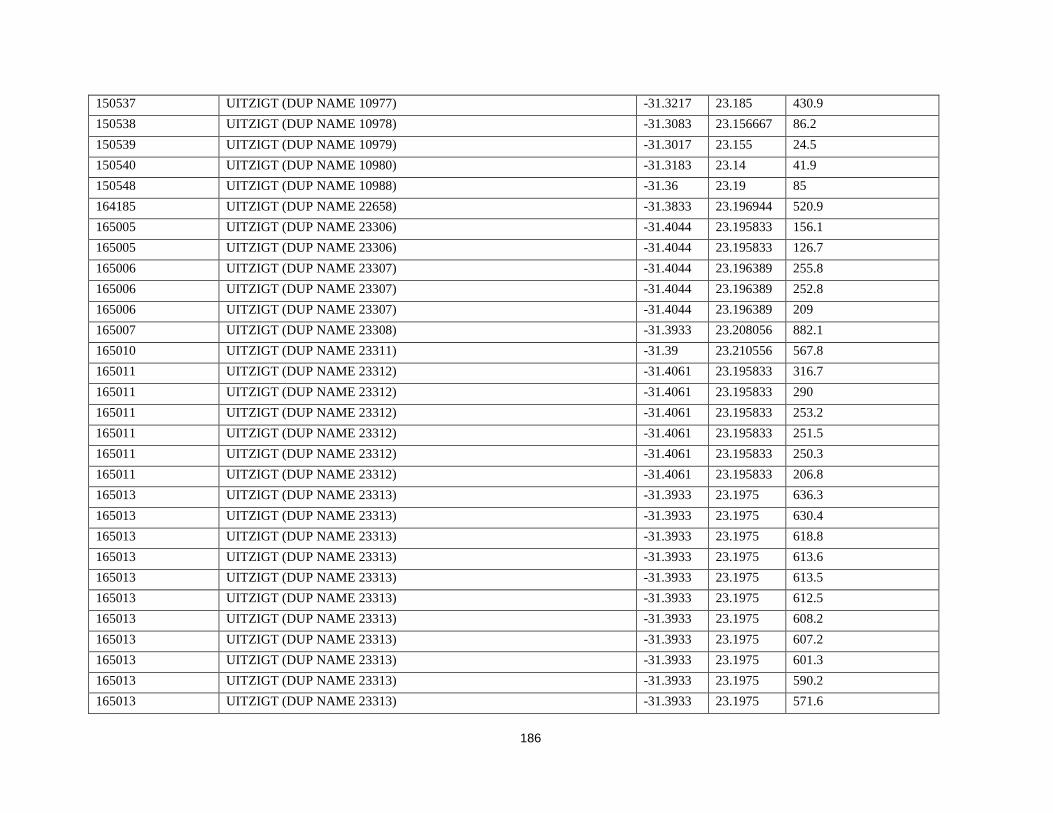
186

150537 UITZIGT (DUP NAME 10977) -31.3217 23.185 430.9 150538 UITZIGT (DUP NAME 10978) -31.3083 23.156667 86.2 150539 UITZIGT (DUP NAME 10979) -31.3017 23.155 24.5 150540 UITZIGT (DUP NAME 10980) -31.3183 23.14 41.9 150548 UITZIGT (DUP NAME 10988) -31.36 23.19 85 164185 UITZIGT (DUP NAME 22658) -31.3833 23.196944 520.9 165005 UITZIGT (DUP NAME 23306) -31.4044 23.195833 156.1 165005 UITZIGT (DUP NAME 23306) -31.4044 23.195833 126.7 165006 UITZIGT (DUP NAME 23307) -31.4044 23.196389 255.8 165006 UITZIGT (DUP NAME 23307) -31.4044 23.196389 252.8 165006 UITZIGT (DUP NAME 23307) -31.4044 23.196389 209 165007 UITZIGT (DUP NAME 23308) -31.3933 23.208056 882.1 165010 UITZIGT (DUP NAME 23311) -31.39 23.210556 567.8 165011 UITZIGT (DUP NAME 23312) -31.4061 23.195833 316.7 165011 UITZIGT (DUP NAME 23312) -31.4061 23.195833 290 165011 UITZIGT (DUP NAME 23312) -31.4061 23.195833 253.2 165011 UITZIGT (DUP NAME 23312) -31.4061 23.195833 251.5 165011 UITZIGT (DUP NAME 23312) -31.4061 23.195833 250.3 165011 UITZIGT (DUP NAME 23312) -31.4061 23.195833 206.8 165013 UITZIGT (DUP NAME 23313) -31.3933 23.1975 636.3 165013 UITZIGT (DUP NAME 23313) -31.3933 23.1975 630.4 165013 UITZIGT (DUP NAME 23313) -31.3933 23.1975 618.8 165013 UITZIGT (DUP NAME 23313) -31.3933 23.1975 613.6 165013 UITZIGT (DUP NAME 23313) -31.3933 23.1975 613.5 165013 UITZIGT (DUP NAME 23313) -31.3933 23.1975 612.5 165013 UITZIGT (DUP NAME 23313) -31.3933 23.1975 608.2 165013 UITZIGT (DUP NAME 23313) -31.3933 23.1975 607.2 165013 UITZIGT (DUP NAME 23313) -31.3933 23.1975 601.3 165013 UITZIGT (DUP NAME 23313) -31.3933 23.1975 590.2 165013 UITZIGT (DUP NAME 23313) -31.3933 23.1975 571.6

187

165013 UITZIGT (DUP NAME 23313) -31.3933 23.1975 567.2 165014 UITZIGT (DUP NAME 23314) -31.3392 23.2 420.6 165015 UITZIGT (DUP NAME 23315) -31.3933 23.195833 258.6 165015 UITZIGT (DUP NAME 23315) -31.3933 23.195833 252.2 165015 UITZIGT (DUP NAME 23315) -31.3933 23.195833 248.9 165015 UITZIGT (DUP NAME 23315) -31.3933 23.195833 207.5 165021 UITZIGT (DUP NAME 23318) -31.3828 23.197222 413.8 165022 UITZIGT (DUP NAME 23319) -31.4006 23.194167 264.3 165022 UITZIGT (DUP NAME 23319) -31.4006 23.194167 251.4 165022 UITZIGT (DUP NAME 23319) -31.4006 23.194167 249.9 165022 UITZIGT (DUP NAME 23319) -31.4006 23.194167 238.4 165023 UITZIGT (DUP NAME 23320) -31.4064 23.195833 324.2 165023 UITZIGT (DUP NAME 23320) -31.4064 23.195833 297 165023 UITZIGT (DUP NAME 23320) -31.4064 23.195833 288.2 165023 UITZIGT (DUP NAME 23320) -31.4064 23.195833 276.3 165023 UITZIGT (DUP NAME 23320) -31.4064 23.195833 269.6 165023 UITZIGT (DUP NAME 23320) -31.4064 23.195833 264.6 165023 UITZIGT (DUP NAME 23320) -31.4064 23.195833 254.5 165023 UITZIGT (DUP NAME 23320) -31.4064 23.195833 253.3 93881 UITZIGT (DUP NAME 3162) -31.405 23.196389 205.6 93881 UITZIGT (DUP NAME 3162) -31.405 23.196389 201.7 150450 UITZUGT (DUP NAME 10895) -31.3917 23.208333 2347 150453 UITZUGT (DUP NAME 10898) -31.4133 23.173333 188.7 150454 UITZUGT (DUP NAME 10899) -31.37 23.173333 70.3 150460 UITZUGT (DUP NAME 10905) -31.3433 23.198333 47.5 150461 UITZUGT (DUP NAME 10906) -31.3167 23.215 128.7 150462 UITZUGT (DUP NAME 10907) -31.3233 23.231667 109.6 150463 UITZUGT (DUP NAME 10908) -31.3283 23.24 137.4 150465 UITZUGT (DUP NAME 10910) -31.4967 23.213333 200.8 150497 UITZUGT (DUP NAME 10939) -31.375 23.111667 84.4

188

150519 UITZUGT (DUP NAME 10961) -31.32 23.111667 38 150520 UITZUGT (DUP NAME 10962) -31.3383 23.116667 48 150523 UITZUGT (DUP NAME 10965) -31.3683 23.133333 56.4 150609 VAN DER MERWESDAM (DUP NAME 11048) -31.3017 23.256667 80 171873 VICTORIA WEST (DUP NAME 27664) -31.3986 23.090833 569.2 171873 VICTORIA WEST (DUP NAME 27664) -31.3986 23.090833 414.4 174153 VICTORIA WEST ALLOTMENT (DUP NAME 29033) -31.3992 23.089444 595.6 177387 VICTORIA WEST ALLOTMENT (DUP NAME 31085) -31.4378 23.125278 82.6 177388 VICTORIA WEST ALLOTMENT (DUP NAME 31086) -31.4483 23.126111 26.1 177389 VICTORIA WEST ALLOTMENT (DUP NAME 31087) -31.4483 23.125833 45.5 177390 VICTORIA WEST ALLOTMENT (DUP NAME 31088) -31.4483 23.125556 53 180372 VICTORIA WEST ALLOTMENT (DUP NAME 31206) -31.4378 23.125833 17 180372 VICTORIA WEST ALLOTMENT (DUP NAME 31206) -31.4378 23.125833 16.1 180372 VICTORIA WEST ALLOTMENT (DUP NAME 31206) -31.4378 23.125833 15.7 180373 VICTORIA WEST ALLOTMENT (DUP NAME 31207) -31.4378 23.126111 72.8 180373 VICTORIA WEST ALLOTMENT (DUP NAME 31207) -31.4378 23.126111 18 180373 VICTORIA WEST ALLOTMENT (DUP NAME 31207) -31.4378 23.126111 17.2 180373 VICTORIA WEST ALLOTMENT (DUP NAME 31207) -31.4378 23.126111 16.7 180374 VICTORIA WEST ALLOTMENT (DUP NAME 31208) -31.4378 23.126389 16.2 180386 VICTORIA WEST ALLOTMENT (DUP NAME 31219) -31.4483 23.126111 51.9 180386 VICTORIA WEST ALLOTMENT (DUP NAME 31219) -31.4483 23.126111 44.1 180386 VICTORIA WEST ALLOTMENT (DUP NAME 31219) -31.4483 23.126111 42.2 180387 VICTORIA WEST ALLOTMENT (DUP NAME 31220) -31.4483 23.125833 50.7 180387 VICTORIA WEST ALLOTMENT (DUP NAME 31220) -31.4483 23.125833 43.9 180387 VICTORIA WEST ALLOTMENT (DUP NAME 31220) -31.4483 23.125833 37 180387 VICTORIA WEST ALLOTMENT (DUP NAME 31220) -31.4483 23.125833 30.4 180388 VICTORIA WEST ALLOTMENT (DUP NAME 31221) -31.4483 23.125556 60.9 180388 VICTORIA WEST ALLOTMENT (DUP NAME 31221) -31.4483 23.125556 57.8 180388 VICTORIA WEST ALLOTMENT (DUP NAME 31221) -31.4483 23.125556 54.4 180477 VICTORIA WEST ALLOTMENT (DUP NAME 31257) -31.4483 23.125278 58.9

189

180477 VICTORIA WEST ALLOTMENT (DUP NAME 31257) -31.4483 23.125278 54.7 180479 VICTORIA WEST ALLOTMENT (DUP NAME 31258) -31.4483 23.124722 64.5 180479 VICTORIA WEST ALLOTMENT (DUP NAME 31258) -31.4483 23.124722 58.5 146783 VICTORIA WEST ALLOTMENT (DUP NAME 8107) -31.4103 23.145278 178.7 146784 VICTORIA WEST ALLOTMENT (DUP NAME 8108) -31.4419 23.093889 242.1 146785 VICTORIA WEST ALLOTMENT (DUP NAME 8109) -31.4417 23.066389 81.7 146786 VICTORIA WEST ALLOTMENT (DUP NAME 8110) -31.3861 23.115278 171.7 146787 VICTORIA WEST ALLOTMENT (DUP NAME 8111) -31.4 23.090556 467.5 146788 VICTORIA WEST ALLOTMENT (DUP NAME 8112) -31.3942 23.0875 42.4 146957 VICTORIA WEST ALLOTMENT (DUP NAME 8224) -31.4169 23.105556 237.8 146958 VICTORIA WEST ALLOTMENT (DUP NAME 8225) -31.4167 23.105833 285.6 146959 VICTORIA WEST ALLOTMENT (DUP NAME 8226) -31.4122 23.109167 908.8 147889 VICTORIA WEST ALLOTMENT (DUP NAME 8902) -31.4378 23.125833 17.5 147890 VICTORIA WEST ALLOTMENT (DUP NAME 8903) -31.4378 23.126111 179.9 147891 VICTORIA WEST ALLOTMENT (DUP NAME 8904) -31.4378 23.126389 15.8 163971 VICTORIA-WES MEENT (DUP NAME 22478) -31.4344 23.089444 145.6 163972 VICTORIA-WES MEENT (DUP NAME 22479) -31.4236 23.080556 126.9 163973 VICTORIA-WES MEENT (DUP NAME 22480) -31.3989 23.076944 119 163974 VICTORIA-WES MEENT (DUP NAME 22481) -31.3861 23.116667 213.6 163974 VICTORIA-WES MEENT (DUP NAME 22481) -31.3861 23.116667 188.3 163974 VICTORIA-WES MEENT (DUP NAME 22481) -31.3861 23.116667 187 165025 VICTORIA-WES MEENT (DUP NAME 23322) -31.4 23.090833 675 165026 VICTORIA-WES MEENT (DUP NAME 23323) -31.395 23.073889 52.2 165027 VICTORIA-WES MEENT (DUP NAME 23324) -31.4108 23.105 1161.6 165028 VICTORIA-WES MEENT (DUP NAME 23325) -31.4108 23.104167 1049.4 151091 VLOOISPOORT (DUP NAME 11495) -31.615 23.031667 107.7 150489 WITVLEI (DUP NAME 10931) -31.4383 23.245 76 165008 WITVLEI (DUP NAME 23309) -31.3933 23.216111 917.9 165008 WITVLEI (DUP NAME 23309) -31.3933 23.216111 879.9 165009 WITVLEI (DUP NAME 23310) -31.3933 23.223611 1199.5

190

165009 WITVLEI (DUP NAME 23310) -31.3933 23.223611 996.8 165009 WITVLEI (DUP NAME 23310) -31.3933 23.223611 579.7 89799 ZQMVWT1 3123AC00018 VICTORIA WEST ALLOTMENT AREA -

VW7 -31.3986 23.090833 719.294

89799 ZQMVWT1 3123AC00018 VICTORIA WEST ALLOTMENT AREA - VW7

-31.3986 23.090833 707.2


-31.3986 23.090833 684.607


-31.3986 23.090833 663.2


-31.3986 23.090833 654.9


-31.3986 23.090833 628.68


-31.3986 23.090833 609.152


-31.3986 23.090833 601.4


-31.3986 23.090833 582.246


-31.3986 23.090833 530.6


-31.3986 23.090833 512.906


-31.3986 23.090833 481.9


-31.3986 23.090833 477.991


-31.3986 23.090833 476.386


-31.3986 23.090833 475.252


-31.3986 23.090833 449.338


-31.3986 23.090833 421.255


-31.3986 23.090833 416.653

191


-31.3986 23.090833 410.1


-31.3986 23.090833 409.9


-31.3986 23.090833 395.4


-31.3986 23.090833 345


-31.3986 23.090833 293.454


-31.3986 23.090833 288.144


-31.3986 23.090833 287.19


-31.3986 23.090833 211.576


-31.3986 23.090833 192.137


-31.3986 23.090833 118.855


-31.3986 23.090833 108.436


-31.3986 23.090833 103.585

Harmonic Mean 69.66500098

192

APPENDIX G: OTHER ACTIVITIES IN THE PROSPECTING AREA

Karoo Array Telescope

A world-class radio telescope was designed in order to accomplish revolutionary science. This

telescope, the MeerKAT Array, is currently being planned in the Karoo region of South Africa

and will be the biggest and most responsive operating radio telescope in the southern hemisphere

of the globe, awaiting the Square Kilometre Array (SKA) which will completed around 2024.

MeerKAT will be commissioned in 2014 and 2015, and will come online for science practices in

2016. The region with the most receivers will be constructed about 80 km from Carnarvon, a

town in the Northern Cape Province. This time slot overlaps with the initiation of the fracking

projects which is also prospected in the Karoo region. The array telescope project involves many

international institutions, researchers and investors and therefore the influence that fracking will

have on the environment of the Karoo raises concerns as these people would want to be certain

of all the potential hazards and risks which may hamper this big and globally important project.

13 countries and almost 100 organisations are already involved. The numbers, joining the project

continues to increase (SKA South Africa, 2013).

MeerKAT will include 64 large antennas, each with a diameter of 13.5m which will be linked

together via optic fibre cables and therefore covering a maximum baseline of 20 km. The parties

involved in the fracking projects must take the area occupied for this project into consideration

and also the consequences fracking might cause in this environment as there will be many

investors and institutions which would expect a fit and suitable site (SKA South Africa, 2013).

The construction of the array will be completed in 2024 and until then the environment and

surrounding projects should reside in proper state to accommodate the project and keep investors

interested (Business Report, 2012 and SKA South Africa, 2013).

Modelling of the impacts of fracking on the Karoo groundwater ...

Documents

Transcript of Modelling of the impacts of fracking on the Karoo groundwater ...