Short wave modelling using special nite elements
22
Journal of Computational Acoustics, Vol. 8, No. 1 (2000) 189–210 c IMACS SHORT WAVE MODELLING USING SPECIAL FINITE ELEMENTS OMAR LAGHROUCHE and PETER BETTESS School of Engineering, University of Durham, Durham DH1 3LE, UK Received 15 June 1999 Revised 2 November 1999 The solutions to the Helmholtz equation in the plane are approximated by systems of plane waves. The aim is to develop finite elements capable of containing many wavelengths and therefore sim- ulating problems with large wave numbers without refining the mesh to satisfy the traditional requirement of about ten nodal points per wavelength. At each node of the meshed domain, the wave potential is written as a combination of plane waves propagating in many possible direc- tions. The resulting element matrices contain oscillatory functions and are evaluated using high order Gauss-Legendre integration. These finite elements are used to solve wave problems such as a diffracted potential from a cylinder. Many wavelengths are contained in a single finite element and the number of parameters in the problem is greatly reduced. 1. Introduction This work involves the development of special finite elements in order to solve two- dimensional short wave problems without being constrained by mesh size problems. Our intention is to extend the method to deal with problems of wave reflection, diffraction and refraction in unbounded media. By short waves, we mean that the wavelength is much smaller than any other length dimensions of the problem. Such problems are of great eco- nomic importance in many fields, including acoustics, sonar and radar cross sections. In such problems where the solution is oscillatory, the usual piecewise polynomial spaces can- not resolve the essential features of the solution unless the mesh size is very small or the polynomial degree is very large. In both cases, the computational costs are still too high even for today’s largest computers. The aim is then to develop finite elements which contain many wavelengths rather than several elements per wavelength. The first idea for this development came from Bettess and Zienkiewicz 1 -3 who incorpo- rated the harmonic variation of the potential into the shape function of infinite elements to study the diffraction and refraction of surface waves in unbounded media. They adopted a Galerkin weighting, but the determination of the resulting integral expression proved to be complicated because of oscillatory terms and special integration rules were developed. Astley et al. 4 -6 later modelled the wave envelope of the potential for acoustical radiation problems by using complex conjugate weightings in the finite element scheme. This simpli- fies the integrand greatly so that it can be evaluated using conventional Gauss-Legendre integration. The elements generate Hermitian matrices. Also when using complex conju- gate weightings, in unbounded problems, some line integrals arise at infinity. For a simple 189
-
Upload
independent -
Category
Documents
-
view
0 -
download
0
Transcript of Short wave modelling using special nite elements
March 24, 2000 12:6 WSPC/130-JCA 0010
Journal of Computational Acoustics, Vol. 8, No. 1 (2000) 189–210c© IMACS
SHORT WAVE MODELLING USING SPECIAL FINITE ELEMENTS
OMAR LAGHROUCHE and PETER BETTESS
School of Engineering, University of Durham, Durham DH1 3LE, UK
Received 15 June 1999Revised 2 November 1999
The solutions to the Helmholtz equation in the plane are approximated by systems of plane waves.The aim is to develop finite elements capable of containing many wavelengths and therefore sim-ulating problems with large wave numbers without refining the mesh to satisfy the traditionalrequirement of about ten nodal points per wavelength. At each node of the meshed domain, thewave potential is written as a combination of plane waves propagating in many possible direc-tions. The resulting element matrices contain oscillatory functions and are evaluated using highorder Gauss-Legendre integration. These finite elements are used to solve wave problems such as adiffracted potential from a cylinder. Many wavelengths are contained in a single finite element andthe number of parameters in the problem is greatly reduced.
1. Introduction
This work involves the development of special finite elements in order to solve two-
dimensional short wave problems without being constrained by mesh size problems. Our
intention is to extend the method to deal with problems of wave reflection, diffraction and
refraction in unbounded media. By short waves, we mean that the wavelength is much
smaller than any other length dimensions of the problem. Such problems are of great eco-
nomic importance in many fields, including acoustics, sonar and radar cross sections. In
such problems where the solution is oscillatory, the usual piecewise polynomial spaces can-
not resolve the essential features of the solution unless the mesh size is very small or the
polynomial degree is very large. In both cases, the computational costs are still too high
even for today’s largest computers. The aim is then to develop finite elements which contain
many wavelengths rather than several elements per wavelength.
The first idea for this development came from Bettess and Zienkiewicz1−3 who incorpo-
rated the harmonic variation of the potential into the shape function of infinite elements
to study the diffraction and refraction of surface waves in unbounded media. They adopted
a Galerkin weighting, but the determination of the resulting integral expression proved to
be complicated because of oscillatory terms and special integration rules were developed.
Astley et al.4−6 later modelled the wave envelope of the potential for acoustical radiation
problems by using complex conjugate weightings in the finite element scheme. This simpli-
fies the integrand greatly so that it can be evaluated using conventional Gauss-Legendre
integration. The elements generate Hermitian matrices. Also when using complex conju-
gate weightings, in unbounded problems, some line integrals arise at infinity. For a simple
189
March 24, 2000 12:6 WSPC/130-JCA 0010
190 O. Laghrouche & P. Bettess
one-dimensional example problem, Bettess7 applied the wave envelope element method to
test infinite wave elements. It was shown that the method yields the exact answer and that
it has many advantages compared to the usual method where the potential is descritized or
usual shape functions are used as weighting.
Bettess and Chadwick8 considered an equivalent approach to that of Astley and applied
it to some simple one-variable propagating wave problems in which both the harmonic time
dependence and fine harmonic detail were removed before discretization. They found that
there was no need to alter the shape functions and they used the standard ones within the
Galerkin finite element scheme in the equivalent approach. The method has been successfully
tested and the progressive short waves were modelled with elements of length much greater
than the wavelength (standing wave problems were also solved in unpublished work). But,
although in one-dimensional wave problems the wave direction is implicitly known, in two-
and three-variable wave problems the wave direction is also an unknown and has to be
determined along with the wave envelope. To do this, they later developed an iteration
procedure for two-dimensional wave problems9 whereby an estimate of the phase is first given
and from the resulting finite element calculation for the wave envelope a better estimate
for the phase is obtained. This method has been used in conjuction with new mapped wave
envelope infinite elements to study the diffraction of short waves in infinite media.10 The
authors investigated the relation between the convergence of the method and the wave
number. They found that for an estimate of the phase, the method will not converge beyond
a certain value of the wave number.
In the present work, the same general way of investigating short waves is followed. But
instead of considering the wave envelope and the phase and then iterating as in previous
work,9,10 we try to approximate solutions of the Helmholtz equation with plane waves whose
vectors encompass all possible directions. It was shown that there are methods for synthetiz-
ing fundamental solutions starting from plane waves and that these constitute complete
systems.11,12 The main idea of c-complete systems, or following the terminology proposed
by Zienkiewicz,13 T -complete systems, to honour Trefftz,14 is to approximate solutions of a
boundary value problem using sets of functions already satisfying the differential equation.
This scheme is generally known as the Trefftz method and has been used in fields such as
the Laplace’s equation, biharmonic equation and elasticity problems.
In the case of the Helmholtz equation, Cheung et al.15 applied the Trefftz method con-
nected to a Galerkin finite element method for calculating wave forces on an offshore struc-
ture in the form of a vertical cylinder. They used series of Hankel functions of the first
kind to approximate the scattered wave potential. In the same kind of application, Stojek16
developed Trefftz-type finite elements where the interelement continuity was performed by a
least-square procedure. It was shown that the required accuracy can be obtained by increas-
ing the number of the subdomains or that of the Trefftz functions. Melenk and Babuska17−19
presented a new finite element method named the Partition of Unity Finite Element Method
(PUFEM) and applied it to solve the Helmholtz equation with high wave numbers. A sum-
mary of this method is given in the textbook of Ihlenburg.20 Its performance was compared
March 24, 2000 12:6 WSPC/130-JCA 0010
Short Wave Modelling Using Special Finite Elements 191
to the performance of the Trefftz method on a two-dimensional model problem by Ihlenburg
and Babuska.21
The elements used and described in this paper are those of Melenk and Babuska. The
ideas involved have evolved with contributions from many authors. The main contributions
are as follows:
• The basic finite element concept from Clough and others, described in the textbook by
Zienkiewicz and Taylor.13
• The introduction of Trefftz type solutions by Trefftz.14
• The demonstration by Herrera et al.11,12 that plane waves, propagating in different direc-
tions form a complete set of functions for Helmholtz equation, using Trefftz type methods.
• The introduction of trigonometrical functions in the single radial direction in infinite
elements by Bettess and Zienkiewicz.1−3
• The introduction of trigonometrical functions in the single radial direction in finite ele-
ments (wave envelope elements) by Astley.4−6
• The introduction of trigonometrical functions representing plane waves in multiple direc-
tions for finite elements, under the methodology of the Partition of Unity Finite Element
Method, by Melenk and Babuska.17−19 The concept of multiple wave directions as a basis
has also been used by de la Bourdonnaye22,23 but not in a classical finite element form.
He gives no numerical results.
Solving wave problems satisfying the Helmholtz equation with finite elements containing
many wavelengths is the main objective of this work. First, the formulation of the finite
element model is described. Then, a few solved examples and a simple convergence study
are presented. Finally, the problem of a plane wave diffracted by a vertical cylinder is solved
using a coarse mesh. The wave number is increased while the mesh size is kept unchanged.
2. Formulation of the problem
2.1. Governing equations and residual scheme
We derive the governing differential equation from the time dependent wave equation24
given by
∂2Φ
∂t2= c2∇2Φ (2.1)
for the time dependent wave potential Φ(x, y, t), where x and y are the two-dimensional
cartesian coordinates, t is the time variable, c is a constant defined as the wave speed and
∇2 is the Laplacian operator. We assume that the time variation is such that Φ = φe−iωt
where φ is a function of x and y, and ω is the circular frequency. Hence the time independent
wave potential φ is given by the Helmholtz equation
(∇2 + k2)φ = 0 on Ω (2.2)
March 24, 2000 12:6 WSPC/130-JCA 0010
192 O. Laghrouche & P. Bettess
where k = ω/c is the wave number and Ω is the studied domain. We assume also that it
satisfies the following Robin boundary condition
∂φ
∂n+ ikφ = g in Γ (2.3)
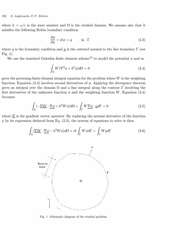
where g is the boundary condition and n is the outward normal to the line boundary Γ (see
Fig. 1).
We use the standard Galerkin finite element scheme13 to model the potential φ and so∫ΩW (∇2φ+ k2φ)dΩ = 0 (2.4)
gives the governing finite element integral equation for the problem whereW is the weighting
function. Equation (2.4) involves second derivatives of φ. Applying the divergence theorem
gives an integral over the domain Ω and a line integral along the contour Γ involving the
first derivatives of the unknown function φ and the weighting function W . Equation (2.4)
becomes ∫Ω
(−∇W · ∇φ+ k2Wφ)dΩ +
∫ΓW∇φ · ndΓ = 0 (2.5)
where ∇ is the gradient vector operator. By replacing the normal derivative of the function
φ by its expression deduced from Eq. (2.3), the system of equations to solve is then∫Ω
(∇W · ∇φ− k2Wφ)dΩ + ik
∫ΓWφdΓ =
∫ΓWgdΓ (2.6)
Fig. 1. Schematic diagram of the studied problem.
March 24, 2000 12:6 WSPC/130-JCA 0010
Short Wave Modelling Using Special Finite Elements 193
2.2. The finite element model
The domain Ω of Fig. 1 is meshed into n-noded finite elements. The unknown function φ
within each element is approximated using polynomial shape functions Nj and the nodal
values of the potential φj as follows
φ =n∑j=1
Njφj (2.7)
It was shown, in the case of the Helmholtz equation, that the system of functions
Jn(kr) cos(nα), Jn(kr) sin(nα), n = 0, 1, 2, . . . (2.8)
is a c-complete system in any bounded region and so the system of plane waves
eikr cos(α−θl), l = 1, 2, 3, . . . (2.9)
is also a c-complete system in any such region.11,12 Essentially because any Bessel function
can be replaced by a set of plane waves. The set of angles θ1, θ2, . . . is dense in [0, 2π], r and α
are the polar coordinates and Jn(kr) is the Bessel function of the first kind and order n. The
proof of c-completeness is beyond the scope of this work and can be found in Refs. 11 and 12.
Let ψ1, ψ2, . . . , ψm bem plane waves and A1j , A
2j , . . . , A
mj be the coefficients, associated with
the node j, corresponding to the plane waves respectively. Then the global approximation
space is given by
φ =n∑j=1
m∑l=1
NjψlAlj (2.10)
where
ψl = eik(x cos θl+y sin θl) (2.11)
This is equivalent to saying that the potential at each node j is expanded in terms of m
unknowns Alj with respect to m directions
φj =m∑l=1
Aljeik(x cos θl+y sin θl) (2.12)
where
θl = l2π
m(2.13)
with l = 1, 2, . . . , m. This means that a separate wave potential is retained for each possible
wave direction. So if waves are allowed at intervals of 10, there would be 36 complex
variables at each node. These m unknowns Alj , in a sense, represent the amplitudes of the
plane waves ψl, l = 1, 2, . . . , m, at the node j. From an approximation point of view, it is
not necessary that the directions are uniformly varied as given in expression (2.13) although
March 24, 2000 12:6 WSPC/130-JCA 0010
194 O. Laghrouche & P. Bettess
this was done by Melenk and Babuska. It is a reasonable thing to do if the actual wave
direction is unknown. But, if the wave solution φ has a preferred direction, it would be
better, a priori, to cluster the angles θl around that direction. For notational convenience,
let us put the “new shape functions” P(j−1)m+l as a product of the “old shape functions”
Nj and the plane waves ψl with j = 1, 2, . . . , n and l = 1, 2, . . . , m.
P(j−1)m+l = Njψl (2.14)
The expression (2.10) of the potential through an n-noded finite element can be written in
a matrix form as
φ =[P1 P2 · · · Pn
]A1
A2...
An
(2.15)
where the row matrix of the new shape functions corresponding to the node j is
Pj =[P(j−1)m+1 P(j−1)m+2 · · ·Pjm
](2.16)
The amplitude vector Aj at the node j, with respect to the directions θ1, θ2, . . . , θm, is
Aj =
A1j
A2j
...
Amj
(2.17)
In the case of the usual piecewise approximation of expression (2.7), the element matrices
would be of dimensions n by n and the unknowns are the nodal values of the potential φj ,
j = 1, 2, . . . , n. However, the resulting element matrices given by the current formulation
are of dimensions (n×m) by (n×m) and the unknowns of the problem are the amplitudes
Alj, j = 1, 2, . . . , n and l = 1, 2, . . . , m. The reader’s first impression may be that this
increases the number of degrees of freedom of the nodes and consequently the dimension of
the whole problem will go up. Actually, the element matrices dimension grows, but as will be
shown in the numerical results, these special finite elements can contain many wavelengths
and this leads to a great reduction in the dimensions of the solved problem.
2.3. Element matrices and numerical integration
The global coordinates x and y of each n-noded finite element are related to the local
coordinates ξ and η using the following transformation
x =n∑j=1
Mjxj , y =n∑j=1
Mjyj (2.18)
March 24, 2000 12:6 WSPC/130-JCA 0010
Short Wave Modelling Using Special Finite Elements 195
where xj and yj are the nodal coordinates and Mj, j = 1, 2, . . . , n, are the shape func-
tions written in local coordinates and are taken to be identical to the shape functions Nj.
To evaluate the element matrices resulting from expression (2.6), the global derivatives of
the new shape fuctions P(j−1)m+l are evaluated from the old shape functions Nj and the
trigonometric functions ψl∂P(j−1)m+l
∂x
∂P(j−1)m+l
∂y
=
∂Nj
∂x
∂Nj
∂y
+ ikNj
cos θlsin θl
ψl (2.19)
The global derivatives of the old shape functions are obtained from the local derivatives∂Nj
∂x
∂Nj
∂y
= J−1
∂Nj
∂ξ
∂Nj
∂η
(2.20)
and the element of surface dxdy is written using local coordinates
dxdy = |J |dξdη (2.21)
where |J | is the determinant of the Jacobian matrix of the geometrical transformation (2.18)
and J−1 is its inverse. The Eq. (2.6) yields then a set of discrete equations of the form
[[K]− k2[M ] + ik[C]]A = F (2.22)
By choosing Galerkin weighting functions, the element matrices are obtained by performing
the integrals
Krs =
∫Ω∇Wr · ∇PsdΩ (2.23)
Mrs =
∫ΩWrPsdΩ (2.24)
Crs =
∫ΓWrPsdΓ (2.25)
and
Fr =
∫ΓWrgdΓ (2.26)
where r and s are integers equal to 1, 2, . . . , (n×m).
The solution A of the system (2.22) contains the coefficients Alj at each node of the
studied domain and with respect to each chosen direction. When calculating the element
matrices, the integrals encountered are of the form
Ijl =
∫ 1
−1
∫ 1
−1f(ξ, η)eik(x cos θj+y sin θj)eik(x cos θl+y sin θl)dξdη (2.27)
March 24, 2000 12:6 WSPC/130-JCA 0010
196 O. Laghrouche & P. Bettess
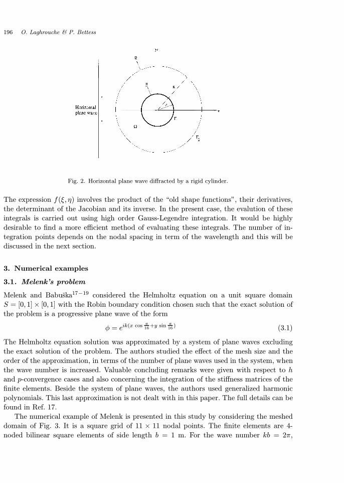
Fig. 2. Horizontal plane wave diffracted by a rigid cylinder.
The expression f(ξ, η) involves the product of the “old shape functions”, their derivatives,
the determinant of the Jacobian and its inverse. In the present case, the evalution of these
integrals is carried out using high order Gauss-Legendre integration. It would be highly
desirable to find a more efficient method of evaluating these integrals. The number of in-
tegration points depends on the nodal spacing in term of the wavelength and this will be
discussed in the next section.
3. Numerical examples
3.1. Melenk’s problem
Melenk and Babuska17−19 considered the Helmholtz equation on a unit square domain
S = [0, 1]× [0, 1] with the Robin boundary condition chosen such that the exact solution of
the problem is a progressive plane wave of the form
φ = eik(x cos π16
+y sin π16
) (3.1)
The Helmholtz equation solution was approximated by a system of plane waves excluding
the exact solution of the problem. The authors studied the effect of the mesh size and the
order of the approximation, in terms of the number of plane waves used in the system, when
the wave number is increased. Valuable concluding remarks were given with respect to h
and p-convergence cases and also concerning the integration of the stiffness matrices of the
finite elements. Beside the system of plane waves, the authors used generalized harmonic
polynomials. This last approximation is not dealt with in this paper. The full details can be
found in Ref. 17.
The numerical example of Melenk is presented in this study by considering the meshed
domain of Fig. 3. It is a square grid of 11 × 11 nodal points. The finite elements are 4-
noded bilinear square elements of side length b = 1 m. For the wave number kb = 2π,
March 24, 2000 12:6 WSPC/130-JCA 0010
Short Wave Modelling Using Special Finite Elements 197
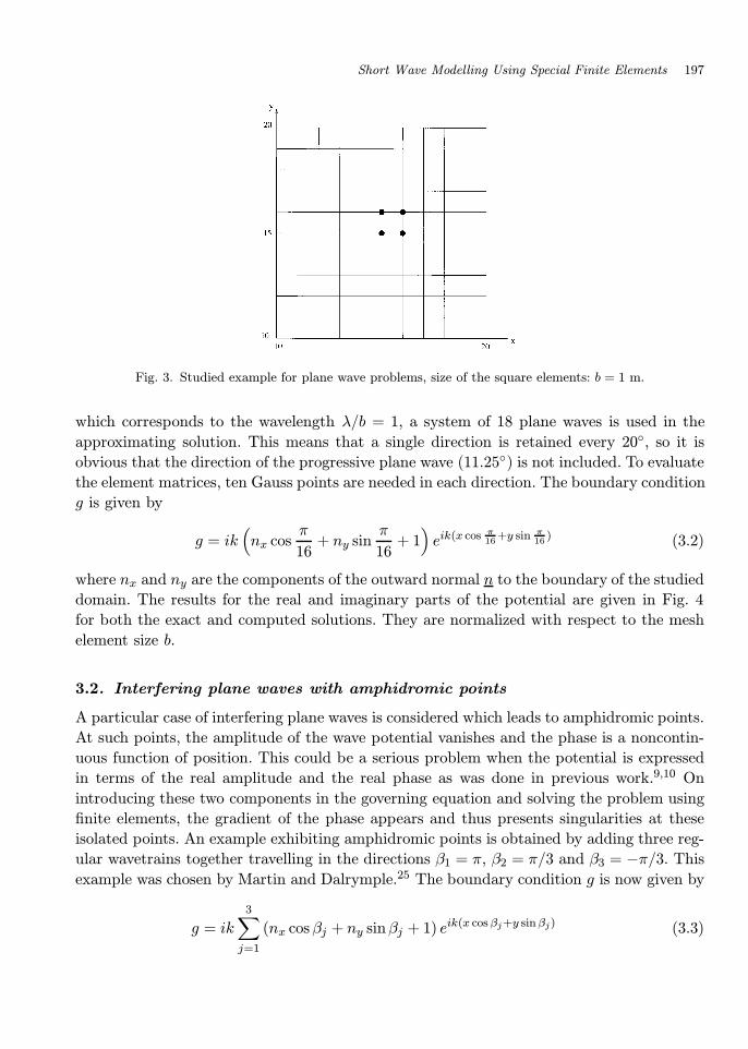
Fig. 3. Studied example for plane wave problems, size of the square elements: b = 1 m.
which corresponds to the wavelength λ/b = 1, a system of 18 plane waves is used in the
approximating solution. This means that a single direction is retained every 20, so it is
obvious that the direction of the progressive plane wave (11.25) is not included. To evaluate
the element matrices, ten Gauss points are needed in each direction. The boundary condition
g is given by
g = ik(nx cos
π
16+ ny sin
π
16+ 1)eik(x cos π
16+y sin π
16) (3.2)
where nx and ny are the components of the outward normal n to the boundary of the studied
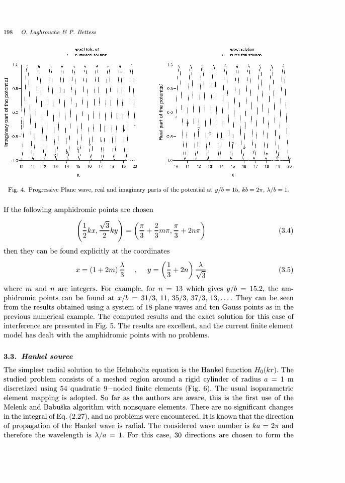
domain. The results for the real and imaginary parts of the potential are given in Fig. 4
for both the exact and computed solutions. They are normalized with respect to the mesh
element size b.
3.2. Interfering plane waves with amphidromic points
A particular case of interfering plane waves is considered which leads to amphidromic points.
At such points, the amplitude of the wave potential vanishes and the phase is a noncontin-
uous function of position. This could be a serious problem when the potential is expressed
in terms of the real amplitude and the real phase as was done in previous work.9,10 On
introducing these two components in the governing equation and solving the problem using
finite elements, the gradient of the phase appears and thus presents singularities at these
isolated points. An example exhibiting amphidromic points is obtained by adding three reg-
ular wavetrains together travelling in the directions β1 = π, β2 = π/3 and β3 = −π/3. This
example was chosen by Martin and Dalrymple.25 The boundary condition g is now given by
g = ik
3∑j=1
(nx cosβj + ny sinβj + 1) eik(x cos βj+y sinβj) (3.3)
March 24, 2000 12:6 WSPC/130-JCA 0010
198 O. Laghrouche & P. Bettess
Fig. 4. Progressive Plane wave, real and imaginary parts of the potential at y/b = 15, kb = 2π, λ/b = 1.
If the following amphidromic points are chosen(1
2kx,
√3
2ky
)=
(π
3+
2
3mπ,
π
3+ 2nπ
)(3.4)
then they can be found explicitly at the coordinates
x = (1 + 2m)λ
3, y =
(1
3+ 2n
)λ√3
(3.5)
where m and n are integers. For example, for n = 13 which gives y/b = 15.2, the am-
phidromic points can be found at x/b = 31/3, 11, 35/3, 37/3, 13, . . . . They can be seen
from the results obtained using a system of 18 plane waves and ten Gauss points as in the
previous numerical example. The computed results and the exact solution for this case of
interference are presented in Fig. 5. The results are excellent, and the current finite element
model has dealt with the amphidromic points with no problems.
3.3. Hankel source
The simplest radial solution to the Helmholtz equation is the Hankel function H0(kr). The
studied problem consists of a meshed region around a rigid cylinder of radius a = 1 m
discretized using 54 quadratic 9−noded finite elements (Fig. 6). The usual isoparametric
element mapping is adopted. So far as the authors are aware, this is the first use of the
Melenk and Babuska algorithm with nonsquare elements. There are no significant changes
in the integral of Eq. (2.27), and no problems were encountered. It is known that the direction
of propagation of the Hankel wave is radial. The considered wave number is ka = 2π and
therefore the wavelength is λ/a = 1. For this case, 30 directions are chosen to form the
March 24, 2000 12:6 WSPC/130-JCA 0010
Short Wave Modelling Using Special Finite Elements 199
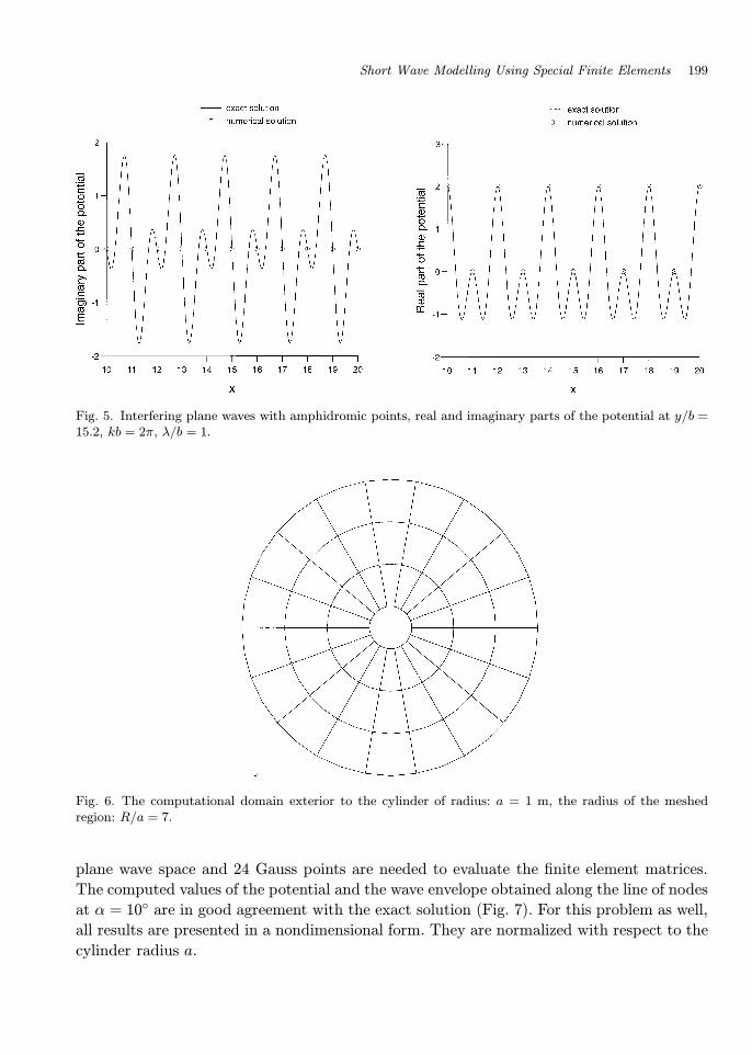
Fig. 5. Interfering plane waves with amphidromic points, real and imaginary parts of the potential at y/b =15.2, kb = 2π, λ/b = 1.
Fig. 6. The computational domain exterior to the cylinder of radius: a = 1 m, the radius of the meshedregion: R/a = 7.
plane wave space and 24 Gauss points are needed to evaluate the finite element matrices.
The computed values of the potential and the wave envelope obtained along the line of nodes
at α = 10 are in good agreement with the exact solution (Fig. 7). For this problem as well,
all results are presented in a nondimensional form. They are normalized with respect to the
cylinder radius a.
March 24, 2000 12:6 WSPC/130-JCA 0010
200 O. Laghrouche & P. Bettess
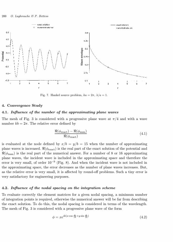
Fig. 7. Hankel source problem, ka = 2π, λ/a = 1.
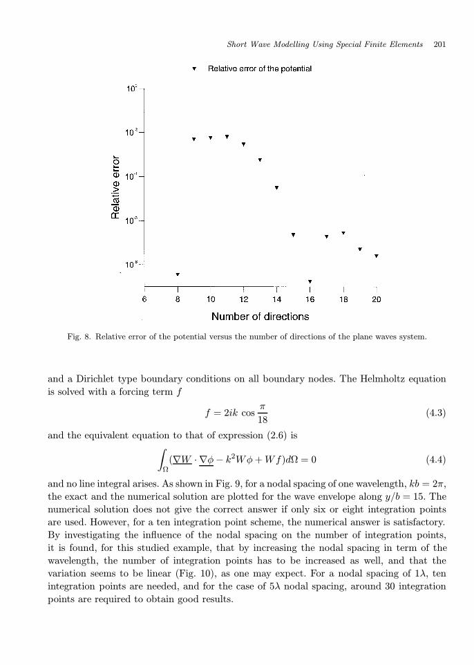
4. Convergence Study
4.1. Influence of the number of the approximating plane waves
The mesh of Fig. 3 is considered with a progressive plane wave at π/4 and with a wave
number kb = 2π. The relative error defined by
<(φexact)−<(φnum)
<(φexact)(4.1)
is evaluated at the node defined by x/b = y/b = 15 when the number of approximating
plane waves is increased. <(φexact) is the real part of the exact solution of the potential and
<(φnum) is the real part of the numerical answer. For a number of 8 or 16 approximating
plane waves, the incident wave is included in the approximating space and therefore the
error is very small, of order 10−9 (Fig. 8). And when the incident wave is not included in
the approximating space, the error decreases as the number of plane waves increases. But,
as the relative error is very small, it is affected by round-off problems. Such a tiny error is
very satisfactory for engineering purposes.
4.2. Influence of the nodal spacing on the integration scheme
To evaluate correctly the element matrices for a given nodal spacing, a minimum number
of integration points is required, otherwise the numerical answer will be far from describing
the exact solution. To do this, the nodal spacing is considered in terms of the wavelength.
The mesh of Fig. 3 is considered with a progressive plane wave of the form
φ = xeik(x cos π18
+y sin π18
) (4.2)
March 24, 2000 12:6 WSPC/130-JCA 0010
Short Wave Modelling Using Special Finite Elements 201
Fig. 8. Relative error of the potential versus the number of directions of the plane waves system.
and a Dirichlet type boundary conditions on all boundary nodes. The Helmholtz equation
is solved with a forcing term f
f = 2ik cosπ
18(4.3)
and the equivalent equation to that of expression (2.6) is∫Ω
(∇W · ∇φ− k2Wφ+Wf)dΩ = 0 (4.4)
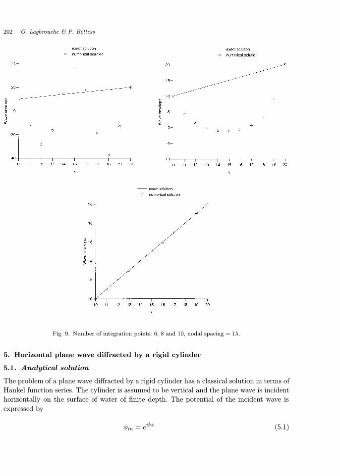
and no line integral arises. As shown in Fig. 9, for a nodal spacing of one wavelength, kb = 2π,
the exact and the numerical solution are plotted for the wave envelope along y/b = 15. The
numerical solution does not give the correct answer if only six or eight integration points
are used. However, for a ten integration point scheme, the numerical answer is satisfactory.
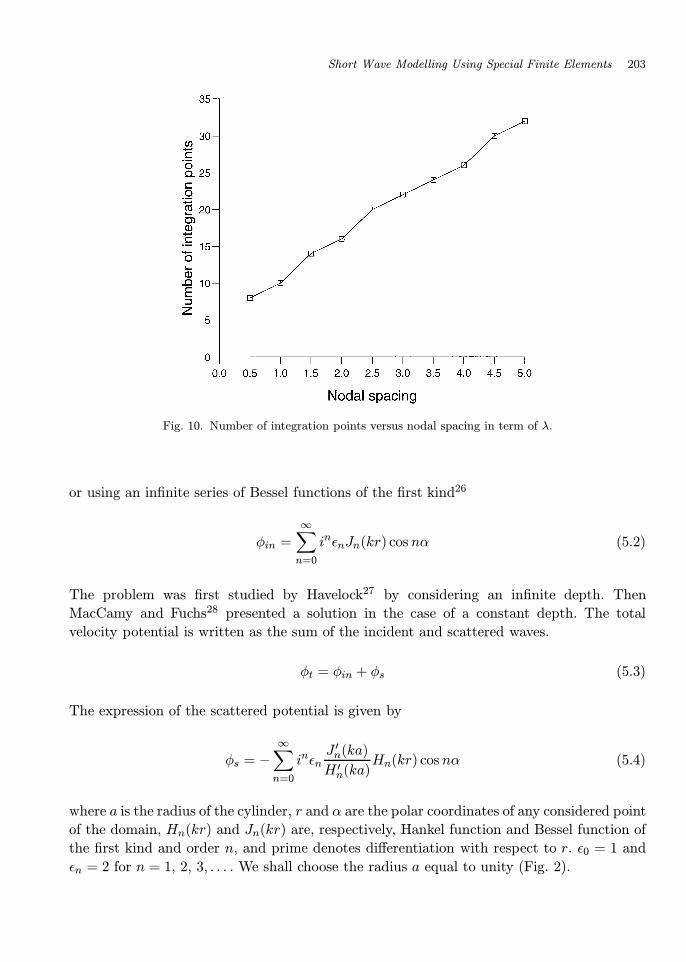
By investigating the influence of the nodal spacing on the number of integration points,
it is found, for this studied example, that by increasing the nodal spacing in term of the
wavelength, the number of integration points has to be increased as well, and that the
variation seems to be linear (Fig. 10), as one may expect. For a nodal spacing of 1λ, ten
integration points are needed, and for the case of 5λ nodal spacing, around 30 integration
points are required to obtain good results.
March 24, 2000 12:6 WSPC/130-JCA 0010
202 O. Laghrouche & P. Bettess
Fig. 9. Number of integration points: 6, 8 and 10, nodal spacing = 1λ.
5. Horizontal plane wave diffracted by a rigid cylinder
5.1. Analytical solution
The problem of a plane wave diffracted by a rigid cylinder has a classical solution in terms of
Hankel function series. The cylinder is assumed to be vertical and the plane wave is incident
horizontally on the surface of water of finite depth. The potential of the incident wave is
expressed by
φin = eikx (5.1)
March 24, 2000 12:6 WSPC/130-JCA 0010
Short Wave Modelling Using Special Finite Elements 203
Fig. 10. Number of integration points versus nodal spacing in term of λ.
or using an infinite series of Bessel functions of the first kind26
φin =∞∑n=0
inεnJn(kr) cos nα (5.2)
The problem was first studied by Havelock27 by considering an infinite depth. Then
MacCamy and Fuchs28 presented a solution in the case of a constant depth. The total
velocity potential is written as the sum of the incident and scattered waves.
φt = φin + φs (5.3)
The expression of the scattered potential is given by
φs = −∞∑n=0
inεnJ ′n(ka)
H ′n(ka)Hn(kr) cos nα (5.4)
where a is the radius of the cylinder, r and α are the polar coordinates of any considered point
of the domain, Hn(kr) and Jn(kr) are, respectively, Hankel function and Bessel function of
the first kind and order n, and prime denotes differentiation with respect to r. ε0 = 1 and
εn = 2 for n = 1, 2, 3, . . . . We shall choose the radius a equal to unity (Fig. 2).
March 24, 2000 12:6 WSPC/130-JCA 0010
204 O. Laghrouche & P. Bettess
5.2. Numerical solution: Robin Robin boundary conditions
Applying the finite element procedure to this particular problem leads to∫Ω
(−∇W · ∇φ+ k2Wφ)dΩ−∫
Γ1
W∇φ · ndΓ +
∫Γ2
W∇φ · ndΓ = 0 (5.5)
where the normal derivative of the potential at both boundaries Γ1 and Γ2 could be replaced
by its expression deduced from the Robin boundary condition (2.3). This gives∫Ω
(∇W · ∇φ− k2Wφ)dΩ− ik∫
Γ1
WφdΓ + ik
∫Γ2
WφdΓ =
∫Γ2
WgdΓ−∫
Γ1
WgdΓ (5.6)
Both potentials of the incident and scattered waves satisfy the Helmholtz equation (2.2).
Then it is possible to solve the problem by considering only φs and so the boundary condition
g is
g =∂φs∂r
nr +1
r
∂φs∂θ
nθ + ikφs (5.7)
where nr and nθ are the components of the outward normal n to the line boundaries Γ1
and Γ2.
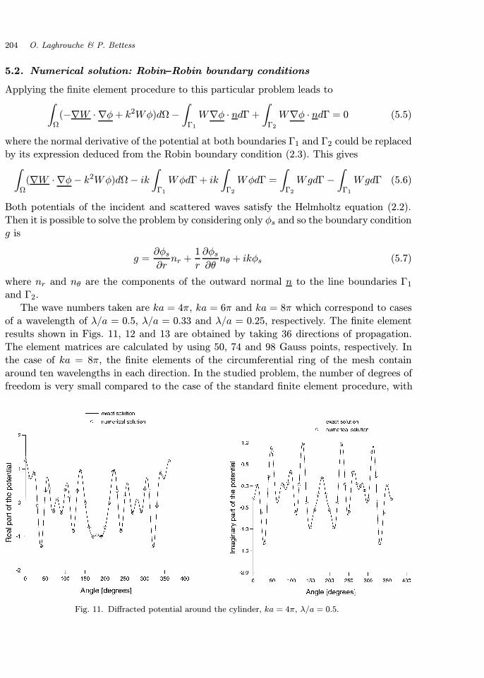
The wave numbers taken are ka = 4π, ka = 6π and ka = 8π which correspond to cases
of a wavelength of λ/a = 0.5, λ/a = 0.33 and λ/a = 0.25, respectively. The finite element
results shown in Figs. 11, 12 and 13 are obtained by taking 36 directions of propagation.
The element matrices are calculated by using 50, 74 and 98 Gauss points, respectively. In
the case of ka = 8π, the finite elements of the circumferential ring of the mesh contain
around ten wavelengths in each direction. In the studied problem, the number of degrees of
freedom is very small compared to the case of the standard finite element procedure, with
Fig. 11. Diffracted potential around the cylinder, ka = 4π, λ/a = 0.5.
March 24, 2000 12:6 WSPC/130-JCA 0010
Short Wave Modelling Using Special Finite Elements 205
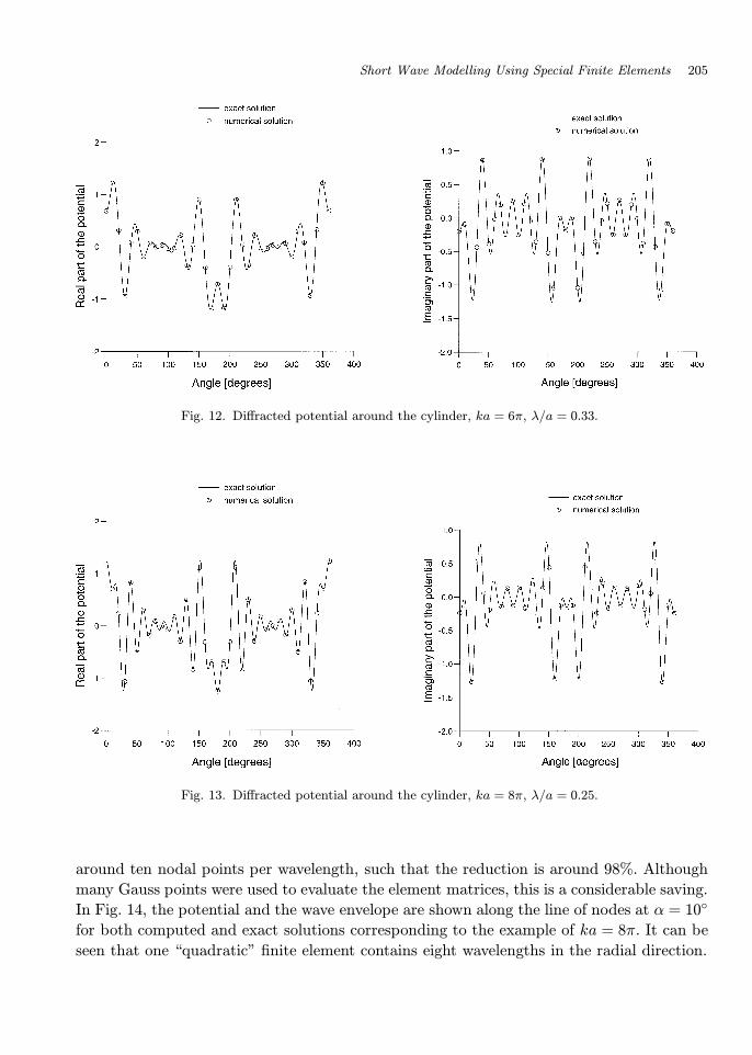
Fig. 12. Diffracted potential around the cylinder, ka = 6π, λ/a = 0.33.
Fig. 13. Diffracted potential around the cylinder, ka = 8π, λ/a = 0.25.
around ten nodal points per wavelength, such that the reduction is around 98%. Although
many Gauss points were used to evaluate the element matrices, this is a considerable saving.
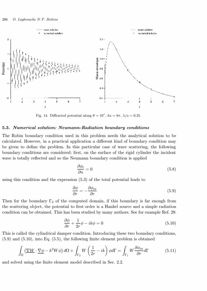
In Fig. 14, the potential and the wave envelope are shown along the line of nodes at α = 10
for both computed and exact solutions corresponding to the example of ka = 8π. It can be
seen that one “quadratic” finite element contains eight wavelengths in the radial direction.
March 24, 2000 12:6 WSPC/130-JCA 0010
206 O. Laghrouche & P. Bettess
Fig. 14. Diffracted potential along θ = 10, ka = 8π, λ/a = 0.25.
5.3. Numerical solution: Neumann-Radiation boundary conditions
The Robin boundary condition used in this problem needs the analytical solution to be
calculated. However, in a practical application a different kind of boundary condition may
be given to define the problem. In this particular case of wave scattering, the following
boundary conditions are considered: first, on the surface of the rigid cylinder the incident
wave is totally reflected and so the Neumann boundary condition is applied
∂φt∂n
= 0 (5.8)
using this condition and the expression (5.3) of the total potential leads to
∂φ
∂r= −∂φin
∂r(5.9)
Then for the boundary Γ2 of the computed domain, if this boundary is far enough from
the scattering object, the potential to first order is a Hankel source and a simple radiation
condition can be obtained. This has been studied by many authors. See for example Ref. 29.
∂φ
∂r+
1
2rφ− ikφ = 0 (5.10)
This is called the cylindrical damper condition. Introducing these two boundary conditions,
(5.9) and (5.10), into Eq. (5.5), the following finite element problem is obtained∫Ω
(∇W · ∇φ− k2Wφ
)dΩ +
∫Γ2
W
(1
2r− ik
)φdΓ =
∫Γ1
W∂φin∂r
dΓ (5.11)
and solved using the finite element model described in Sec. 2.2.
March 24, 2000 12:6 WSPC/130-JCA 0010
Short Wave Modelling Using Special Finite Elements 207
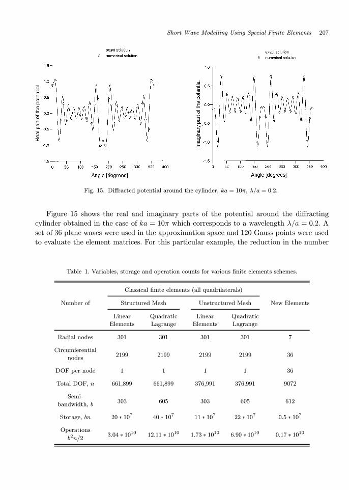
Fig. 15. Diffracted potential around the cylinder, ka = 10π, λ/a = 0.2.
Figure 15 shows the real and imaginary parts of the potential around the diffracting
cylinder obtained in the case of ka = 10π which corresponds to a wavelength λ/a = 0.2. A
set of 36 plane waves were used in the approximation space and 120 Gauss points were used
to evaluate the element matrices. For this particular example, the reduction in the number
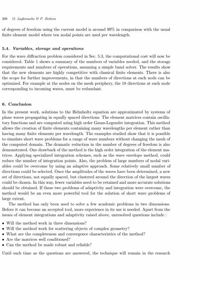
Table 1. Variables, storage and operation counts for various finite elements schemes.
Classical finite elements (all quadrilaterals)
Number of Structured Mesh Unstructured Mesh New Elements
Linear Quadratic Linear Quadratic
Elements Lagrange Elements Lagrange
Radial nodes 301 301 301 301 7
Circumferential2199 2199 2199 2199 36nodes
DOF per node 1 1 1 1 36
Total DOF, n 661,899 661,899 376,991 376,991 9072
Semi-303 605 303 605 612bandwidth, b
Storage, bn 20 ∗ 107 40 ∗ 107 11 ∗ 107 22 ∗ 107 0.5 ∗ 107
Operations3.04 ∗ 1010 12.11 ∗ 1010 1.73 ∗ 1010 6.90 ∗ 1010 0.17 ∗ 1010
b2n/2
March 24, 2000 12:6 WSPC/130-JCA 0010
208 O. Laghrouche & P. Bettess
of degrees of freedom using the current model is around 99% in comparison with the usual
finite element model where ten nodal points are used per wavelength.
5.4. Variables, storage and operations
For the wave diffraction problem considered in Sec. 5.3, the computational cost will now be
considered. Table 1 shows a summary of the numbers of variables needed, and the storage
requirements and numbers of operations, assuming a simple band solver. The results show
that the new elements are highly competitive with classical finite elements. There is also
the scope for further improvements, in that the numbers of directions at each node can be
optimized. For example at the nodes on the mesh periphery, the 18 directions at each node
corresponding to incoming waves, must be redundant.
6. Conclusion
In the present work, solutions to the Helmholtz equation are approximated by systems of
plane waves propagating in equally spaced directions. The element matrices contain oscilla-
tory functions and are computed using high order Gauss-Legendre integration. This method
allows the creation of finite elements containing many wavelengths per element rather than
having many finite elements per wavelength. The examples studied show that it is possible
to simulate short wave problems for a range of wave numbers without changing the mesh of
the computed domain. The dramatic reduction in the number of degrees of freedom is also
demonstrated. One drawback of the method is the high order integration of the element ma-
trices. Applying specialized integration schemes, such as the wave envelope method, could
reduce the number of integration points. Also, the problem of large numbers of nodal vari-
ables could be overcome by using an adaptive approach. Some relatively small number of
directions could be selected. Once the amplitudes of the waves have been determined, a new
set of directions, not equally spaced, but clustered around the direction of the largest waves
could be chosen. In this way, fewer variables need to be retained and more accurate solutions
should be obtained. If these two problems of adaptivity and integration were overcome, the
method would be an even more powerful tool for the solution of short wave problems of
large extent.
The method has only been used to solve a few academic problems in two dimensions.
Before it can become an accepted tool, more experience in its use is needed. Apart from the
issues of element integrations and adaptivity raised above, unresolved questions include :
• Will the method work in three dimensions?
• Will the method work for scattering objects of complex geometry?
• What are the completeness and convergence characteristics of the method?
• Are the matrices well conditioned?
• Can the method be made robust and reliable?
Until such time as the questions are answered, the technique will remain in the research
March 24, 2000 12:6 WSPC/130-JCA 0010
Short Wave Modelling Using Special Finite Elements 209
domain. However, the results to date are encouraging enough to hope that the method will
be further investigated and developed.
Acknowledgments
We are grateful to the EPSRC for funding the work in this paper through Grant
No. GR/K81652 and GR/M41025. We are also grateful to Dr. Edmund Chadwick, whose
earlier work helped in these developments, for useful discussions. Peter Bettess acknowledges
with grateful thanks the assistance of Durham University, in awarding him a Sir Derman
Christopherson Fellowship for the academic year 1999–2000.
References
1. O. C. Zienkiewicz and P. Bettess, “Infinite elements in the study of fluid-structure interactionproblems,” Computing Methods in Applied Sciences, Lecture Notes in Physics 58 (Springer-Verlag, Berlin, 1975), pp. 133–169.
2. P. Bettess and O. C. Zienkiewicz, “Diffraction and refraction of surface waves using finite andinfinite elements,” Int. J. Num. Meth. Eng. 11 (1977), 1271–1290.
3. O. C. Zienkiewicz, K. Bando, P. Bettess, C. Emson, and T. C. Chiam, “Mapped infinite elementsfor exterior wave problems,” Int. J. Num. Meth. Eng. 21 (1985), 1229–1251.
4. R. J. Astley, “Wave envelope and infinite elements for acoustical radiation,” Int. J. Num. Meth.Flu. 3 (1983), 507–526.
5. R. J. Astley and W. Eversman, “Finite element formulation for acoustical radiation,” J. SoundVib. 88 (1983), 47–64.
6. R. J. Astley, G. J. Macaulay, and J. P. Coyette, “Mapped wave envelope elements for acousticalradiation and scattering,” J. Sound Vib. 170 (1994), 97–118.
7. P. Bettess, “A simple wave envelope element example,” Comm. Appl. Numer. Methods 3 (1987),77–80.
8. P. Bettess and E. A. Chadwick, “Wave envelope examples for progressive waves,” Int. J. Num.Meth. Eng. 38 (1995), 2487–2508.
9. E. A. Chadwick and P. Bettess, “Modelling of progressive short waves using wave envelopes,”Int. J. Num. Meth. Eng. 40 (1997), 3229–3245.
10. E. A. Chadwick, P. Bettess, and O. Laghrouche, “Diffraction of short waves modelled usingnew mapped wave envelope finite and infinite elements,” Int. J. Num. Meth. Eng. 45 (1999),335–354.
11. I. Herrera and F. J. Sabena, “Connectivity as an alternative to boundary integral equations,”Proc. Natl. Acad. Sci. USA 75 (1978), 2059–2063.
12. F. J. Sanchez-Sesma, I. Herrera, and J. Aviles, “A boundary method for elastic wave diffraction:application to scattering of SH waves by surface irregularities,” Bull. Seism. Soc. Am. 72 (1982),491–506.
13. O. C. Zienkiewicz and R. L. Taylor, The Finite Element Method (McGrawHill, London, 1989).14. E. Trefftz, “Ein Gegenstuck zum Ritz’schen Verfahren,” Proc. 2nd Int. Congr. Appl. Mech.,
Zurich (1926), 131–137.15. Y. K. Cheung, W. G. Jin and O. C. Zienkiewicz, “Solution of Helmholtz equation by Trefftz
method,” Int. J. Num. Meth. Eng. 32 (1991), 63–78.16. M. Stojek, “Least-squares Trefftz-type elements for the Helmholtz equation,” Int. J. Num. Meth.
Eng. 41 (1998), 831–849.
March 24, 2000 12:6 WSPC/130-JCA 0010
210 O. Laghrouche & P. Bettess
17. J. M. Melenk, “On generalized Finite Element Methods,” Ph.D. Thesis, (University of Maryland,1995).
18. J. M. Melenk and I. Babuska, “The Partition of Unity Finite Element Method. Basic theory andapplications,” Comput. Meths. Appl. Mech. Eng. 139 (1996), 289–314.
19. J. M. Melenk and I. Babuska, “The Partition of Unity Method,” Int. J. Num. Meth. Eng. 40(1997), 727–758.
20. F. Ihlenburg, Finite Element Analysis of Acoustic Scattering (Springer-Verlag, New York, 1998).21. F. Ihlenburg and I. Babuska, “Solution of Helmholtz problems by knowledge-based FEM,” Comp.
Ass. Mech. Eng. Sci. 4 (1997), 397–415.22. A. de la Bourdonnaye, “High frequency approximation of integral equations modeling scattering
phenomena,” Mathematical Modelling and Numerical Analysis 28 (1994), 223–241.23. A. de la Bourdonnaye, “Une methode de discretisation microlocale et son application a un
probleme de diffraction,” C. R. Acad. Sci., Paris, t. 318, Serie I (1994), 385–388.24. H. Lamb, Hydrodynamics (Cambridge University Press, 1932).25. P. A. Martin and R. A. Dalrymple, “On amphidromic points,” Proc. Roy. Soc. Lon., Series A
444 (1994), 91–104.26. A. M. Abramowitz and I. A. Stegun, Handbook of Mathematical Functions (Dover Publications,
New York, 1965).27. T. H. Havelock, “The pressure of water waves upon a fixed obstacle,” Proc. Roy. Soc. Lon.,
Series A 963 (1940), 409–421.28. R. C. MacCamy and R. A. Fuchs, “Wave forces on piles. A diffraction theory,” Beach Erosion
Board Tech. Mem. No. 69 (1954).29. K. Bando, P. Bettess, and C. Emson, “The effectiveness of dampers for the analysis of exterior
scalar wave diffraction by cylinders and ellipsoids,” Int. J. Num. Meth. Eng. 4 (1984), 599–617.