GOVERNMENT CONSUMPTION AND THE COMPOSITION OF PRIVATE EXPENDITURE: A CONDITIONAL ERROR CORRECTION...

GOVERNMENT CON SUMPT I ON ANDTHE COMPO S I T I ON OF PR I VATEEX P END I TURE : A COND I T I ONAL

ERROR CORRECT I ON MODEL

David Aristein and Luca Pieronin

Abstract

In this paper we provide empirical evidence of the relationship between government

purchases and private expenditure by adopting a microeconomic approach. Using

UK quarterly data, a long-run demand system conditioned to the public sector is

obtained by specifying a vector error correction model in which government

consumption is assumed as an exogenous I(1) forcing variable. Our findings reject

the hypothesis of separability of individual preferences between public and private

expenditures, with simultaneous crowding-out/in effects. Moreover, crowding-out

effects of government consumption on private spending are found to be larger for

those goods and services that produce similar utility.

I Introduction

A central issue in macroeconomic analysis is testing the presence of a direct

channel of influence of fiscal policy on private consumption decisions. The

assumption that aggregate private consumption remains unaffected by a change

in government expenditure has been proved to be questionable. Empirical

investigations have shown that government expenditures exert a significant

influence on private consumption behaviour (Kormendi, 1983; Aschauer, 1985;

Ni, 1995; Kuehlwein, 1998). Moreover, when government consumption is

decomposed into functional categories, the results concerning the impact of

public expenditures are mixed, revealing the existence of both substitutability

and complementarity effects (Graham, 1993; Karras, 1994; Kuehlwein, 1998;

Fiorito and Kollintzas, 2004).

However, the empirical macroeconomic literature has devoted little attention

to the impact of government spending on the allocation of private consumption.

As suggested by Aschauer (1993), a more profitable approach would also involve

a decomposition of both private consumption and public spending in a way that

might allow cleaner substitutability tests.

In this paper, a micro-based framework is used to derive a dynamic demand

system conditioned to the public sector directly from a utility-maximization

nDepartment of Economics, Finance and Statistics, University of Perugia.

Scottish Journal of Political Economy, Vol. 55, No. 2, May 2008r 2008 The AuthorsJournal compilation r 2008 Scottish Economic Society. Published by Blackwell Publishing Ltd,9600 Garsington Road, Oxford, OX4 2DQ, UK and 350 Main St, Malden, MA, 02148, USA

143

process, offering the opportunity to investigate the impact of different

government expenditure changes on disaggregate private spending. Accordingly,

we devote our attention to explaining how a conditional error correction model

is appropriate. From a theoretical point of view, the quantities of publicly

provided goods and services are predetermined with respect to consumer

choices. Under the assumption of non-stationarity, this allows to specify a long-

run conditional demand system in which government expenditure enters as an

I(1) forcing variable (Johansen, 1992; Boswijk, 1994, 1995; Urbain, 1995; Harbo

et al., 1998).

In this framework, the inclusion of government expenditures as structurally

exogenous variables enables long-run substitutability/complementarity effects

with private expenditures to be recovered (Pieroni and Aristei, 2005). In

particular, the flexibility of the cost function, which generates a first-order

approximation of the private demand system, enables to estimate consistently

the complementarity and substitutability relationships between public expendi-

ture and private consumption in each period of the sample.

In the empirical section, we use quarterly UK data for the period 1964Q1–

2002Q4, adopting a functional classification of private expenditures to obtain a

demand system that includes three macro-categories of goods: (1) Health,

Education, Social Protection, Recreation and Culture (HER); (2) Other

Services; and (3) Food, Energy and other non-durables. Government

expenditures are represented by ‘Total public consumption’ (G), which is then

decomposed into ‘Individual public consumption’ (GI) and ‘Collective public

consumption’ (GC).

The main objectives of the analysis are to test whether private decisions are

affected by government allocation and to verify simultaneously the presence of

crowding-out/in effects in different categories of private spending. In particular,

it is worth investigating how the ‘HER’ category responds to changes in

government allocations because the relationship between those private and

public categories that produce similar utility has not been tested exhaustively.

Finally, in order to obtain a consistent comparison with the macroeconomic

literature, we build an aggregate indicator of crowding-out starting from the

substitution elasticities of government expenditures on the disaggregate demand

system.

The rest of the paper is organized as follows. Section II outlines the

theoretical framework based on the analysis of consumer behaviour under

rationing. In Section III, a long-run conditional Almost Ideal demand system is

derived as a partial vector autoregressive model. In Section IV, we present the

empirical results. Section IV.1 discusses data and time series properties. Section

IV.2 reports the estimation results, while Section IV.3 assesses the relationships

between private and public expenditures. Section V concludes the paper.

II Theory

A formal way of testing the impact of the public provision of goods and services

on private consumption is represented by the specification of a flexible demand

D. ARISTEI AND L. PIERONI144

r 2008 The AuthorsJournal compilation r 2008 Scottish Economic Society

system, extended to the public sector, in which government expenditures enter

consumer utility function in a non-separable way. In empirical demand studies,

the utility conferred on consumers by publicly provided goods and services is

usually disregarded and separability of individual preferences between private

and public consumption is implicitly assumed.

Unlike private expenditures, the public provision of goods and services,

although directly conferring utility on the consumer, is not freely chosen but

established a priori by the government. The level and composition of public

spending, as well as the taxes needed to finance those expenditures, are therefore

exogenous from the consumer viewpoint. Given this setting, the theory of

consumer behaviour under quantity constraints (Pollak, 1969, 1971; Neary and

Roberts, 1980; Deaton, 1981; Deaton and Muellbauer, 1981) can be applied to

derive demand functions for private goods conditioned to publicly provided items

and to analyze the influence of public consumption on private expenditures.

In order to derive the conditional demand functions, following Pollak (1969),

we consider a class of freely purchased goods whose n � 1 vectors of quantities

and prices are denoted as y and p, respectively. We then define the class of

rationed goods whose preferences are not parameterized and whose consump-

tion is pre-determined in the quantity z at the fixed price r. The cost function

c�ðu; p; r; zÞ can be defined as the minimum cost needed to obtain the utility level

u, given the price vectors p and r when the quantity z of the rationed good must

be purchased. Formally:

c�ðu; p; r; zÞ ¼ miny

r0zþ p0yjuðy; zÞ ¼ u�; z ¼ z�½ �;

¼ r0z� þminy

p0qjuðy; zÞ ¼ u�½ �;

¼ r0z� þ gðu; p; z�Þ;

ð1Þ

where gðu; p; z�Þ is the conditional cost function. From the cost function (1), a

conditional demand system can be derived. Firstly, it should be noted that the

price of the rationed good (r) enters the cost function only through the fixed

term r0z�. For this reason the conditional compensated (Hicksian) demand

functions, obtained as the gradient of c�ðu; p; r; zÞ with respect to p, do not

depend on r:

@c�ðu; p; r; zÞ@p

¼ hðu; p; zÞ ¼ y: ð2Þ

Inverting the cost function (1) and substituting it into the compensated

demands (2), we obtain the conditional uncompensated (Marshallian) demand

functions, which relate y to prices p, to total expenditure e and to the quantity of

the ration z:

y ¼ gðe; p; zÞ; ð3Þ

where q represents the n � 1 partitioned quantity vector of the freely purchased

goods.

GOVERNMENT CONSUMPTION 145


This framework can be adopted to analyze the relationships between private

and public consumption. Denoting as Y the n � 1 vector of privately purchased

goods and as G the m � 1 vector of quantities of publicly provided goods and

services, the consumer utility maximization problem becomes:

max u ¼ uðY ;GÞ½ � s:t: Y 0P ¼ E; ð4Þ

where P represents the vector of prices of the freely chosen goods and E equals

disposable income, because G is assumed to be entirely financed by tax revenue.

By solving the constrained maximization problem (4), we derive the following

uncompensated conditional demand function:

Y ¼ gðE;P;GÞ: ð5Þ

The public provision of goods and services exerts two effects on the demand

for privately purchased goods: an income effect, whereby an increase in the

public provision financed by taxation reduces the amount of income available to

purchase freely chosen items, and a substitution/complementarity effect,

whereby the consumer rearranges his expenditure on freely chosen goods

following a change in the quantity constraint.

Therefore, the standard demand function Y ¼ gðE;PÞ is simply a special case

of function (5), which is only correct when public consumption G is separable

from private expenditures Y. Our aim is therefore to verify the possibility of

restricting the conditional demand function (5) and to test for separability

between private and public consumption.

In order to derive the separability test, we have to first define a specific

functional form in which public consumption enters the utility function in a non-

separable way; otherwise, by construction, public consumption will not influence

consumer behaviour and the effect of public purchases will be reduced to an

income effect only, with private expenditures decreasing as government

spending, and hence its financing through taxation, grows (Tridimas, 2002).

Moreover, the functional form adopted should be as flexible as possible to allow

the analysis of all the possible interactions between private and public

expenditures (Levaggi, 1998, 1999). The Almost Ideal Demand System (Deaton

and Muellbauer, 1980) seems to be the most appropriate specification, because it

provides a first-order approximation of any demand system and allows a wide

range of substitution effects. Following Tridimas (2002), the cost function of the

conditional Almost Ideal model can be written as

log Cðu;P;GÞ ¼ a0 þXni¼1

ai þXmj¼1

yijGj

!log Pi

þ 1

2

Xni¼1

Xmk¼1

g�ik log Pi log Pk þ uðY ;GÞb0Yni¼1

Pbii :

ð6Þ

Minimizing the cost function Cðu;P;GÞ, given the market prices of

the privately purchased goods, yields the demand equations in terms of



budget shares:

wi ¼ai þXnk¼1

gik lnPk þ bi log E � log P½ �

þXmj¼1

yijGj; i; k ¼ 1; 2; . . . ; n; j ¼ 1; 2; . . . ;m;

ð7Þ

where gik ¼ ð1=2Þðg�ik þ g�kiÞ, Pk is the relative price of the kth good, X represents

the total expenditure, log P ¼ a0 þPn

i¼1 ai þPm

j¼1 yijGj

� �log Pi þ ð1=2ÞPn

i¼1Pm

j¼1 gik log Pi log Pk is a functional form usually approximated by the

Stone indexPn

i¼1 wi log Pi

� �and Gj represents real public expenditures. The

theoretical constraints of adding up, homogeneity and symmetry imply the

following restrictions directly on the parameters of the model:

Adding up:Xiai ¼ 1;

Xigik ¼ 0;

Xibi ¼ 0;

Xiyij ¼ 0; 8k; j: ð8Þ

Homogeneity:Xkgik ¼ 0; 8i: ð9Þ

Symmetry:

gik ¼ gki; 8i; k: ð10Þ

Unlike homogeneity and symmetry, the adding-up constraint is not testable

and is automatically satisfied, given that the budget shares sum to one. The

restrictions in (8) make the variance–covariance matrix singular and to solve this

problem an arbitrary equation must be omitted from the system, so that only

n� 1 non-singular equations are estimated.

Given this setting, separability of consumer preferences between private and

public goods can be verified by checking the statistical significance of the yijparameters. The introduction of G as an additional element of equation (7)

further allows to measure the direct effect of public consumption on each

category of private spending by means of the elasticity of the demand for Yi with

respect to Gj ðeij ¼ yijGj=wiÞ.

III Econometric Model

In this section, we define the properties of a partial VAR model to estimate the

relationship between private and government expenditures. As in the previous

static demand system, government expenditure variables are modelled as

conditioning goods. The motivation to use a conditional subsystem in demand

analysis stems from the traditional in which the set of variables under

investigation, xt, is usually partitioned between the so-called endogenous

variables, yt, and those whose generating process will not be modelled, the

exogenous variables zt.



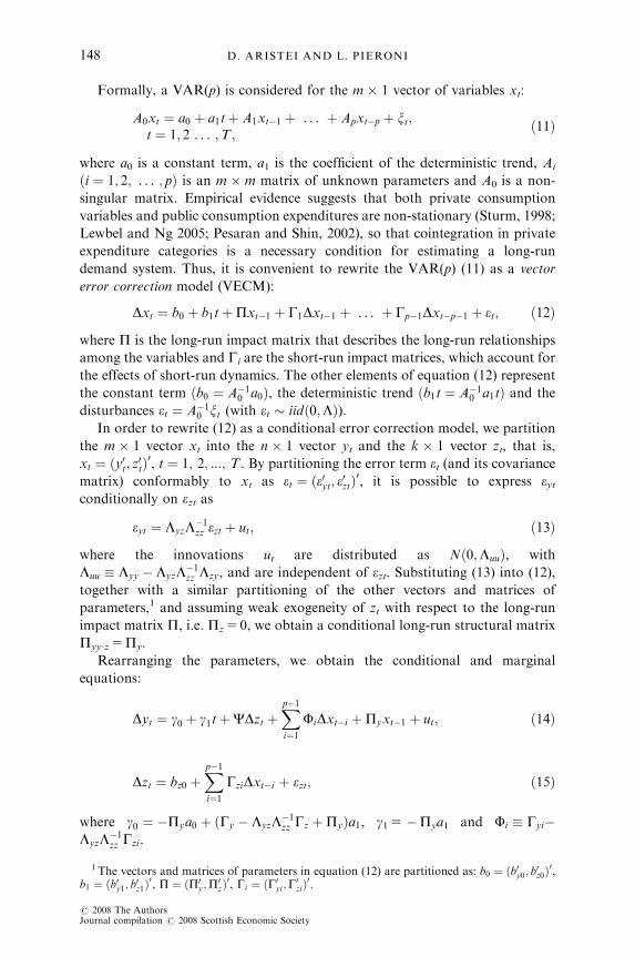
Formally, a VAR(p) is considered for the m � 1 vector of variables xt:

A0xt ¼ a0 þ a1tþ A1xt�1 þ . . . þ Apxt�p þ xt;t ¼ 1; 2 . . . ;T ;

ð11Þ

where a0 is a constant term, a1 is the coefficient of the deterministic trend, Ai

ði ¼ 1; 2; . . . ; pÞ is an m � m matrix of unknown parameters and A0 is a non-

singular matrix. Empirical evidence suggests that both private consumption

variables and public consumption expenditures are non-stationary (Sturm, 1998;

Lewbel and Ng 2005; Pesaran and Shin, 2002), so that cointegration in private

expenditure categories is a necessary condition for estimating a long-run

demand system. Thus, it is convenient to rewrite the VAR(p) (11) as a vector

error correction model (VECM):

Dxt ¼ b0 þ b1tþPxt�1 þ G1Dxt�1 þ . . . þ Gp�1Dxt�p�1 þ et; ð12Þ

where P is the long-run impact matrix that describes the long-run relationships

among the variables and Gi are the short-run impact matrices, which account for

the effects of short-run dynamics. The other elements of equation (12) represent

the constant term ðb0 ¼ A�10 a0Þ, the deterministic trend ðb1t ¼ A�10 a1tÞ and the

disturbances et ¼ A�10 xt (with et � iidð0;LÞ).In order to rewrite (12) as a conditional error correction model, we partition

the m � 1 vector xt into the n � 1 vector yt and the k � 1 vector zt, that is,

xt ¼ ðy0t; z0tÞ0, t ¼ 1; 2; :::; T . By partitioning the error term et (and its covariance

matrix) conformably to xt as et ¼ ðe0yt; e0ztÞ0, it is possible to express eyt

conditionally on ezt as

eyt ¼ LyzL�1zz ezt þ ut; ð13Þ

where the innovations ut are distributed as Nð0;LuuÞ, with

Luu � Lyy � LyzL�1zz Lzy, and are independent of ezt. Substituting (13) into (12),

together with a similar partitioning of the other vectors and matrices of

parameters,1 and assuming weak exogeneity of zt with respect to the long-run

impact matrix P, i.e. Pz 5 0, we obtain a conditional long-run structural matrix

Pyy�z 5Py.

Rearranging the parameters, we obtain the conditional and marginal

equations:

Dyt ¼ g0 þ g1tþCDzt þXp�1i¼1

FiDxt�i þPyxt�1 þ ut; ð14Þ

Dzt ¼ bz0 þXp�1i¼1

GziDxt�i þ ezt; ð15Þ

where g0 ¼ �Pya0 þ ðGy � LyzL�1zz Gz þPyÞa1, g1 5 �Pya1 and Fi � Gyi�

LyzL�1zz Gzi.

1 The vectors and matrices of parameters in equation (12) are partitioned as: b0 ¼ ðb0y0; b0z0Þ0,

b1 ¼ ðb0y1; b0z1Þ0, P ¼ ðP0y;P0zÞ

0, Gi ¼ ðG0yi;G0ziÞ0.



The restriction Pz 5 0 clearly excludes cointegrating relationships in the

marginal model (15). Moreover, this restriction makes the information available

from model (15) redundant for efficient estimation and inference on Py as well

as on g0, g1, C and Fi. Thus, in line with Granger and Lin (1995), we define zt as

long-run forcing for yt.

By Granger’s representation theorem constrained to the conditional

model (14), the Py matrix is decomposed as Py 5 ayb0 by the n � r

loadings matrix ay and the m � r matrix of cointegrating vectors b0 (Harbo

et al., 1998).

The cointegration rank hypothesis can be formulated in the context of (14) as

Hr : Rank½Py� ¼ r; r ¼ 0; . . . ; n; ð16Þ

and can be tested under different intercept and trend specifications (Pesaran

et al., 2000).

The assumption of weak exogeneity of zt for b0 enables us to make inference

on the cointegrating vector from the conditional model (14) because it is

assumed that the variables zt do not react to disequilibria. Note that

when a VAR model is formulated, the selection of the variables should be

determined by economic theory. In the conditional long-run demand system,

government expenditures are modelled as a structurally exogenous random

variable, because the public provision of goods and services is predetermined

with respect to consumer choice, which is assumed to have a I(1) data generating

process. Thus, given this specification, the parameters of interest for the

conditional demand system are those included in the cointegrating vectors.

Disregarding deterministic terms, the r cointegrating vectors of the AI model can

be written:

cvðrÞ ¼ b0xt�1¼ b0 w1t�1; . . . ;wn�1t�1; ln p1t�1; . . . ; ln pnt�1; lnðEt�1=Pt�1Þ;Gtð Þ:

ð17Þ

Moreover, a variety of theoretical hypotheses, including substitutability/

complementarity effects between private and public consumption and homo-

geneity and symmetry properties, can be tested by imposing restrictions directly

on b0.The adding-up constraint is crucial for the identification of the long-run

demand system. A sufficient condition to recover a structural demand system

from the data generating process is that the number of cointegrating relation-

ships should be equal to the number of non-singular demand equations

(r5 n� 1) specified in terms of budget shares (wt). The rank condition excludes

all the cases in which ron� 1. With respect to the estimation of a long-run

private demand system (Pesaran and Shin, 2002), the rank test of cointegration

of the Py matrix is performed by introducing government expenditures as

conditioning I(1) variables. The critical values used for the rank cointegration

test with exogenous I(1) are taken from Harbo et al. (1998).



The estimation of the VEC model (14), subject to reduced rank restrictions on

the Py matrix, does not lead to the exact identification of the cointegrating

relations. Given the decompositionP5 ayb0, the identification of the parameters

in b0 requires the imposition of at least r a priori restrictions on each

cointegrating vector. A necessary and sufficient condition for the identification

of the long-run parameters is that rank RðIr � bÞf g ¼ r2; this condition holds,

provided that the number of the identifying restrictions, k, is at least equal to r2

(order condition).

Thus, the exact identification of the cointegrating relationships of a long-run

AI demand system in n equations requires r2 5 (n� 1)2 restrictions on the

parameters of the cointegrating vectors, which are given by

HEI ¼

b11 ¼ �1 b12 ¼ 0 � � � b1n�1 ¼ 0b21 ¼ 0 b22 ¼ �1 � � � b2n�1 ¼ 0

..

. ... . .

. ...

bn�11 ¼ 0 bn�12 ¼ 0 � � � bn�1n�1 ¼ �1

8>>><>>>:

9>>>=>>>;: ð18Þ

Moreover, k� r2 over-identifying restrictions can be imposed and tested. In the

present application, these restrictions may be taken directly from demand

theory. The empirical validity of the theoretical constraints of homogeneity and

symmetry can therefore be verified using the log-likelihood ratio statistic

ðLR ¼ 2½lðHeiÞ � lðHoiÞ�Þ, which is asymptotically distributed as a w2, with

degrees of freedom being equal to the number of over-identifying restrictions

imposed.

Finally, government expenditures enter demand functions as additional

forcing variables, whose legitimate exclusion can be justified only if private

commodity demands are weakly separable from government expenditures.

Separability is proved when the parameter(s) of Gt in the b0 vector are not

statistically significant in modifying private consumption decisions. Conse-

quently, it is possible to restrict the conditional model to a private

demand system. On the contrary, if separability of individual preferences is

rejected, the conditional specification of a long-run demand system is

appropriate.

To sum up, the demand model used in this work is characterized by the

following economic properties: (a) the conditional model leads only private

budget shares to adjust in response to long-run deviations from equilibrium; (b)

demand theory imposes the theoretical restrictions of homogeneity and

symmetry directly on the long-run parameters of the cointegrating vector b0;and (c) government expenditures Gt are modelled as exogenous I(1) forcing

variables, allowing to account for substitutability effects and to test directly for

separability of individual preferences between private and publicly provided

goods. In order to identify the heterogeneous effects of government spending on

private consumption, in the next section we consider different specifications,

which alternatively include total public consumption and individual and

collective government expenditures.



IV Empirical Evidences

Data and time series properties

The conditional long-run Almost Ideal model presented in the previous section

is estimated for a three-commodity demand system using UK quarterly data for

the period 1964–2002. The choice of a high aggregated representation of data is

connected to the data-intensive nature of the VECM approach, which prevents

the correct analysis of demand systems with a large number of consumption

categories. The three private consumption categories that make up the demand

system are: (1) Health, Education, Social Protection, Recreation and Culture; (2)

Services (including rents and rates); and (3) Food, Energy and other non-

durables. The main feature of this functional classification consists in the

aggregation of private expenditures on health, education, recreation and culture

and social protection in a single category. The definition of this particular

category is aimed at the aggregation of all household expenditures on those

goods and services that can also be offered by the public sector.

The private demand system is conditioned by including public expenditures

as rationed quantities in order to test for separability of individual preferences

between private and public consumption items. The Almost Ideal model is firstly

conditioned to total public consumption (G) so as to evaluate the overall effect

of the public provision of goods and services on private consumption behaviour.

Aggregate public consumption is then divided into the categories ‘Individual

public consumption’ (GI), which includes public expenditure on health,

education, social protection, recreation and culture and ‘Collective public

consumption’ (GC), which includes government expenditures on defence, public

order and safety, general public services and justice. This representation of

public expenditures allows us to analyze separately the effects of those goods

and services that are non-rival and non-excludible in consumption from those

that are more akin to private goods (Fiorito and Kollintzas, 2004).

The data used in the empirical application are taken from the UK quarterly

National Accounts, published by the Office for National Statistics (ONS).2 The

series of private consumption expenditures are seasonally adjusted and

expressed both at current and constant 2002 prices. Price indexes for each

commodity group are obtained as implicit deflators of the three expenditure

categories. Private spending is net of durable consumption expenditures, which

are included in some non-food spending components.3 Total expenditure is

transformed into per capita terms, by dividing the original series by resident

2More precisely, private expenditure data are taken from ‘Household final consumptionexpenditure: classified by purpose’ (Blue Book, Tables 6.4 and 6.5), while those concerninggovernment spending are obtained from ‘Gross domestic product: expenditure approach’ (BlueBook, Tables 1.2 and 1.3). Data are freely provided on-line by the UK Office for NationalStatistics (http://www.statistics.gov.uk).

3 The presence of durable components within private consumption may represent a problemfor a correct specification of the demand system, because of the temporal gap between themoment in which those expenditures are made and when they transfer their utility. Supportingarguments for the exclusion of durable expenditures can be found in several studies (Aschauer,1985; Marrinan, 1998; Tridimas, 2002).



population.4 Public consumption expenditures are expressed at constant 2002

prices and transformed into per capita terms.

For the aims of our analysis, an issue with public expenditure data is that

quarterly observations are available for the series of total public consumption only,

while disaggregated information on the composition of public spending is available

on an annual basis. Quarterly data on individual and collective public consumption

are obtained by disaggregating the relative annual series. In particular, we compare

the results obtained by the Chow and Lin (1971), Fernandez (1981), Litterman

(1983) and Santos Silva and Cardoso (2001) methods, including alternative

auxiliary series. The performance of each method has been evaluated by means of

the Akaike Information Criterion (AIC) and of the Root Mean Squared

Percentage Error (RMSPE), computed on both the levels and the growth rates

of each series.5 Based on these indicators, the Litterman (1983) method, including

the quarterly series of aggregate government consumption as a high-frequency

indicator, has been preferred, even if it is worth noticing that the differences in the

performance of the disaggregation methods are relatively small.6

Because the cointegrated VAR analysis pre-assumes the variables of the

demand system to be non-stationary, Augmented Dickey–Fuller (Dickey and

Fuller, 1979) and Phillips–Perron (Phillips and Perron, 1988) tests are computed

to examine whether the time series of the three budget shares (w1t, w2t, w3t), of

the relative prices (log p1t, log p2t, log p3t), of real total expenditure

(logEt� log pt) and of real government expenditures (G, GI and GC) contain

a unit root in their data-generating process. Table 1 summarizes the results of

the ADF and PP tests. Because the results are sensitive to the inclusion of

deterministic components in the test regression, we compute the unit root tests

including both a constant and a linear trend and only a constant in the

underlying regressions; the inclusion of irrelevant deterministic components may

in fact reduce the power of the test to reject the null of a unit root. Moreover, the

number of lagged difference terms in the ADF test regression has been selected

using the Schwarz information criterion so as to remove serial correlation in the

residuals. The results of both the specifications of the ADF and the PP tests

clearly indicate that it is not possible to reject the null hypothesis of unit root at

the 5% and 1% significance levels for any of the variables of the demand system.

Estimating the long-run demand system

In this section, the conditional demand system (14) is estimated using alternative

definitions of public consumption. In particular, assuming non-separability

between private and public goods, two conditional specifications are con-

4Quarterly data on population are obtained by interpolation of annual population figurespublished by ONS.

5All the alternative annual to quarterly estimations of the series of individual and collectivepublic consumption have been carried out by means of the Matlab toolbox written by Abad andQuilis (2005). Complete results and details on the disaggregation methods considered areavailable from the authors.

6 The estimated quarterly series are then adjusted for seasonality by means of the Census X12-ARIMA method.



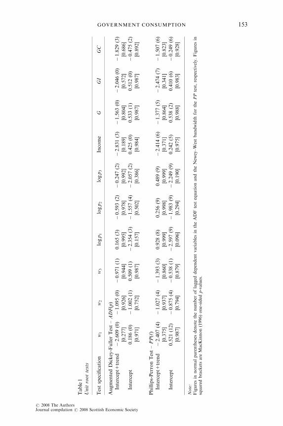
Table1

Unitroottests

Testspecification

w1

w2

w3

logp1

logp2

logp3

Income

GGI

GC

AugmentedDickey-Fuller

Test–ADF(p)

Intercept1

trend�2.609(0)�1.095(0)�0.971(1)

0.165(3)

�0.593(2)�0.247(2)�2.831(3)�1.563(0)�2.046(0)�1.829(3)

[0.277]

[0.926]

[0.944]

[0.995]

[0.978]

[0.992]

[0.189]

[0.804]

[0.572]

[0.686]

Intercept

0.186(0)

�1.002(1)

0.509(1)

�2.354(3)�1.557(4)�2.057(2)

0.425(0)

0.533(1)

0.512(0)

�0.475(2)

[0.971]

[0.752]

[0.987]

[0.157]

[0.502]

[0.386]

[0.984]

[0.987]

[0.987]

[0.892]

Phillips-PerronTest–PP(‘)

Intercept1

trend�2.407(4)�1.027(4)�1.393(3)

0.928(8)

0.256(9)

0.489(9)

�2.414(6)�1.377(5)�2.474(7)�1.507(6)

[0.375]

[0.937]

[0.860]

[0.999]

[0.998]

[0.999]

[0.371]

[0.864]

[0.341]

[0.823]

Intercept

0.521(12)�0.875(4)�0.538(1)�2.597(9)�1.983(9)�2.249(9)

0.242(5)

0.538(2)

0.410(6)

�0.249(6)

[0.987]

[0.794]

[0.879]

[0.096]

[0.294]

[0.190]

[0.975]

[0.988]

[0.983]

[0.928]

Note:

Figuresin

norm

alparentheses

denote

thenumber

oflagged

dependentvariablesin

theADF

test

equationandtheNew

ey–Westbandwidth

forthePP

test,respectively.Figuresin

squaredbracketsare

MacK

innon(1996)one-sided

p-values.



sidered by alternatively including total public consumption (G) and individual

(GI) and collective (GC) government expenditures as exogenous I(1) forcing

variables.

In the estimation of the conditional model, the adding-up restrictions are not

testable and are a priori imposed, requiring a budget share equation to be

omitted from the system. The results are invariant to the choice of the n� 1

equation included in the model. In this analysis, the budget share equation of

Food, Energy and other non-durables (w3) is omitted and its long-run

parameters are then determined from the adding-up constraints.

In order to verify the presence of cointegrating relationships between the

variables of the demand system, it is necessary to solve some preliminary issues

connected with the specification of the VEC model (14). Firstly, we have to

define the order of the autoregressive model. The relatively short length of the

sample size does not allow the use of a large autoregressive dimension.

Moreover, as Boswijk and Franses (1992) and Reimers (1992) show, the

selection of the order p is crucial in the VECM specification because it may affect

the cointegration rank test. In particular, an excessive number of lags lowers the

power of the test, while an underspecification of the VAR order could

potentially lead to the much more relevant problem of spurious cointegration.

The lag order is selected using the AIC, the Schwarz Bayesian Criterion (SBC)

and a small-sample corrected LR test.7 The results are reported in Table 2; as it

Table 2

Lag order selection

Order LL AIC SBC Adjusted LR test

(a) Demand system conditional on G

6 3721.5 3493.5 3151.9 –

5 3701.1 3509.1 3221.3 w2(36)5 30.4567 [.729]

4 3667.8 3511.8 3278.1 w2(72)5 79.8194 [.247]

3 3645.1 3525.1 3345.2 w2(108)5 113.6829 [.335]

2 3619.1 3535.1 3409.2 w2(144)5 152.3419 [.301]

1 3557.5 3509.5 3437.5 w2(180)5 243.8907 [.001]

0 1772 1760 1742 w2(216)5 2898.0 [.000]

(b) Demand system conditional on GI and GC

6 3726.8 3486.8 3127.1 –

5 3705.1 3501.1 3195.4 w2(36)5 31.6760 [.674]

4 3671.2 3503.2 3251.4 w2(72)5 81.1657 [.215]

3 3648 3516 3318.2 w2(108)5 114.9255 [.306]

2 3622.3 3526.3 3382.4 w2(144)5 152.5313 [.297]

1 3561.9 3501.9 3412 w2(180)5 240.5958 [.002]

0 1936.5 1912.5 1876.5 w2(216)5 2612.9 [.000]

Note:AIC, Akaike Information Criterion; SBC, Schwarz Bayesian Criterion. Figures in round parentheses denotethe degrees of freedom of the chi-squared statistics. Figures in squared brackets are adjusted LR testp-values.

7 In selecting the lag order, we do not consider orders 46, because of data limitations.



can be noted, the two information criteria considered and the adjusted LR test

univocally indicate that the optimal lag order, for both the conditional

specifications, is equal to two (p5 2).

Because the cointegrating rank hypothesis depends on deterministic

variables, the reduced rank procedure of Johansen is revised to estimate the

conditional system with these variables included (Pesaran et al., 2000).

Consumer theory predicts that budget shares converge towards a steady-state

value proxied by the constant g0. Thus, we assume a VAR(2) model with

restricted intercepts and no trend to ensure that steady-state values

for the budget shares exist both under the null and the alternative hypo-

thesis (Pesaran and Shin, 2002). Formally, the structural VECM estimated

becomes:

Dyt ¼ ð�Pya0Þ þCDzt þ F1Dxt�1 þPyxt�1 þ ut; ð19Þ

where a0 is the intercept term of the cointegrating relationships.

Only when the model specification is defined, it is possible to determine the

rank of the long-run multiplier matrix Py. The asymptotic distribution of the

LR test statistic for cointegration does not have a standard distribution and

strictly depends on the assumptions made with respect to both the lag length and

the deterministic components of the model. The test for the presence of

cointegrating relationships among the private demand variables is developed by

using the maximal-eigenvalue and trace tests (Johansen, 1995), in which the

critical values are modified to take into account the exogenous I(1) forcing

variables (Harbo et al., 1998). The necessary condition to identify an error

correction demand system requires two cointegrating relationships among the

six endogenous variables of the conditional demand system, corresponding to

the two non-singular budget share equations. The results of the cointegration

tests are presented in Table 3. At the 5% significance level, the maximal-

eigenvalue and the trace statistics unambiguously indicate the presence of two

cointegrating relationships, providing support for the definition of the

conditional cointegrated demand system.

Thus, the necessary condition for the exact identification of the para-

meters of the two cointegrating vectors requires four restrictions to be

imposed; these exact identifying restrictions, implicit in the specification

of the share equations of the AID model, take the following diagonal

structure:

HEI ¼b11 ¼ �1 b12 ¼ 0b21 ¼ 0 b22 ¼ �1

� �: ð20Þ

The exactly identified matrix of long-run parameters will then have a total of five

and six unrestricted parameters to be estimated, respectively, for the demand

systems conditioned to total public consumption and to individual and collective

public expenditures. These unrestricted parameters correspond to the three

prices, to total per-capita expenditure and to the public consumption vari-

ables (G or GI1GC, alternatively), plus the constant terms. The exactly

identified estimates of the two cointegrating vectors are presented in



Table 3

Johansen’s cointegration rank tests


No. of CE(s)

Max-Eigen Statistic 95% critical value 90% critical valueH0 H1

r5 0 r5 1 80.389 43.76 40.93

r 1 r5 2 47.966 37.48 34.99

r 2 r5 3 30.542 31.48 29.01

r 3 r5 4 15.272 25.54 22.98

r 4 r5 5 6.845 18.88 16.74

r 5 r5 6 5.787 12.45 10.50

No. of CE(s)

Trace Statistic 95% critical value 90% critical valueH0 H1

r5 0 r 1 186.801 116.30 110.50

r 1 r 2 106.412 86.58 82.17

r 2 r 3 58.446 62.75 59.07

r 3 r 4 27.904 42.40 39.12

r 4 r 5 12.632 25.23 22.76

r 5 r 6 5.787 12.45 10.50


No. of CE(s)

Max–Eigen Statistic 95% critical value 90% critical valueH0 H1

r5 0 r5 1 80.700 46.90 44.05

r 1 r5 2 51.480 40.57 37.81

r 2 r5 3 29.538 34.69 32.00

r 3 r5 4 17.053 28.49 26.08

r 4 r5 5 7.130 21.92 19.67

r 5 r5 6 4.944 15.27 13.21

No. of CE(s)

Trace Statistic 95% critical value 90% critical valueH0 H1

r5 0 r 1 190.845 128.93 123.48

r 1 r 2 110.145 97.57 92.93

r 2 r 3 58.664 72.15 67.83

r 3 r 4 29.127 49.43 45.89

r 4 r 5 12.074 30.46 27.58

r 5 r 6 4.944 15.27 13.21

Note:The 95% and 90% critical values used for the rank cointegration test with exogenous I(1) are taken fromHarbo et al. (1998).



Table 48; the maximized values of the log-likelihood functions of the exact

identified VEC models, conditional on G and GI1GC, are equal to 3700.7 and

3702.5, respectively.

The homogeneity and symmetry constraints are imposed and tested empirically

as over-identifying restrictions. In particular, the homogeneity constraint implies

the following two restrictions on the long-run parameters:

Hhom ¼b13 þ b14 þ b15 ¼ 0b23 þ b24 þ b25 ¼ 0

� �; ð21Þ

while the symmetry constraint requires the following cross-equation restriction

on the parameters of the two cointegrating vectors:

Hsym ¼ fb14 ¼ b23g: ð22Þ

Table 4

Estimated cointegrating vectors subject to exact identifying restrictions


w1t w2t log p1 log p2 log p3 log (Et/Pt) G Intercept

Cointegrating

Vector 1

� 1 0 � 0.0552 0.2243 � 0.1608 � 0.0940 � 0.0885 0.1781

(0.054) (0.053) (0.043) (0.044) (0.042) (0.042)

Cointegrating

Vector 2

0 � 1 0.2340 � 0.3415 0.1312 0.3981 0.0884 0.4056

(0.123) (0.123) (0.098) (0.101) (0.097) (0.098)


w1t w2t log p1 log p2 log p3 log (Et/Pt) GI GC Intercept

Cointegrating

Vector 1

� 1 0 � 0.0282 0.1968 � 0.1594 � 0.0635 � 0.0583 � 0.0394 0.1929

(0.043) (0.039) (0.037) (0.034) (0.024) (0.017) (0.038)

Cointegrating

Vector 2

0 � 1 0.2117 � 0.3244 0.1354 0.3572 0.0791 0.0392 0.3672

(0.109) (0.101) (0.095) (0.088) (0.064) (0.045) (0.099)

Note:Standard errors in round brackets.

8Using the adding-up constraints, the third cointegrating share equations are given by

w3t ¼ 0:4163ð0:061Þ

� 0:1788ð0:077Þ

log p1 þ 0:1172ð0:077Þ

log p2 þ 0:0295ð0:061Þ

log p3 � 0:3040ð0:063Þ

logðEt=PtÞ

� 0:0001ð0:061Þ

Gt

and

w3t ¼ 0:4399ð0:067Þ

� 0:1835ð0:074Þ

log p1 þ 0:1276ð0:068Þ

log p2 þ 0:0239ð0:066Þ

log p3 � 0:2937ð0:056Þ

logðEt=PtÞ

� 0:0208ð0:043Þ

GIt þ 0:0002ð0:030Þ

GCt

for the demand systems conditioned to G and GI1GC, respectively.



The maximized values of the log-likelihood functions for the two demand

systems conditioned to G and GI1GC, obtained by imposing both the

theoretical restrictions, are equal to 3693.9 and 3694.8, respectively.

The empirical validity of the theoretical constraints of homogeneity and

symmetry is tested using an LR test, based on the log-likelihood values of

the restricted and unrestricted specifications. In finite samples standard

asymptotic results can be misleading, because they are biased towards over-

rejection when the number of equations and parameters of the models is large

with respect to the sample size (Dufour and Khalaf, 2002). In particular, tests

of homogeneity and symmetry in demand systems have proved to be very

sensitive to this problem when models are heavily parameterized (Laitinen,

1978; Pudney, 1981; Theil and Fiebig, 1985). In this analysis, it is therefore

worth implementing a small-sample adjustment to correct the over-rejection

tendency of the LR tests. Following Pudney (1981), we define the adjusted LR

statistic as

LR� ¼ LRþ nT log ðnT � p1Þ=ðnT � p0Þ½ �; ð23Þ

where n is the number of equations and p0 and p1 are the numbers of

parameters of the restricted and unrestricted specifications, respectively. An

analogous correction is also carried out for the critical values, which take the

form K ¼ nT log 1þ dFdnT�p1=ðnT � p1Þ

h i, where d5 p1� p0 and Fd

nT�p1 is the

critical value for the F distribution.

The results of the joint test of homogeneity and symmetry, with and without

small-sample correction, are presented in Table 5. For comparability purposes,

theoretical restrictions have also been tested for the separable demand system to

obtain a comprehensive check of the consistency of demand theory with the

data.

As it is common in demand studies (see Ng, 1995), the joint asymptotic test

for the theoretical restrictions leads to a general rejection of the null hypothesis

in all the three specifications considered, with LR test statistics well above the

corresponding 1% critical value. After applying the small-sample correction, the

test results change, with an evident improvement in the statistical significance of

Table 5

Tests for theoretical restrictions

Model specification

Standard asymptotic results Small-sample correction

LR statistic

[w2ð3Þ] p-value

Test

statistic

5% critical

value

1% critical

value

1. Conditional specifications:

(a) G 13.610 0.003 9.944 8.509 12.488

(b) GI1GC 15.451 0.001 11.507 8.617 12.649

2. Separable specification 20.780 0.000 17.623 8.403 12.331

Note:Small-sample corrected critical values are computed as: K ¼ nT log 1þ dFd

nTp1=ðnT � p1Þ

h i.



the homogeneity and symmetry constraints for the model conditioned to total

public consumption. In particular, the small-sample-adjusted LR tests indicate

that the theoretical restrictions can be rejected at the 5% significance level for all

the specifications considered, even if we are unable to reject homogeneity and

symmetry restrictions at the 1% level of significance in the conditional

specifications.

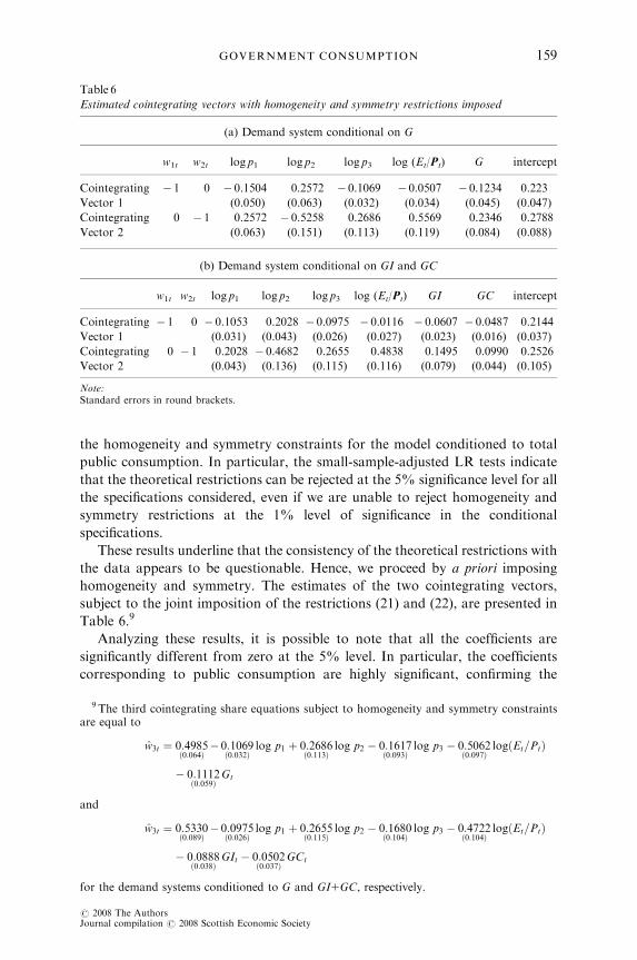
These results underline that the consistency of the theoretical restrictions with

the data appears to be questionable. Hence, we proceed by a priori imposing

homogeneity and symmetry. The estimates of the two cointegrating vectors,

subject to the joint imposition of the restrictions (21) and (22), are presented in

Table 6.9

Analyzing these results, it is possible to note that all the coefficients are

significantly different from zero at the 5% level. In particular, the coefficients

corresponding to public consumption are highly significant, confirming the

Table 6

Estimated cointegrating vectors with homogeneity and symmetry restrictions imposed


w1t w2t log p1 log p2 log p3 log (Et/Pt) G intercept

Cointegrating

Vector 1

� 1 0 � 0.1504 0.2572 � 0.1069 � 0.0507 � 0.1234 0.223

(0.050) (0.063) (0.032) (0.034) (0.045) (0.047)

Cointegrating

Vector 2

0 � 1 0.2572 � 0.5258 0.2686 0.5569 0.2346 0.2788

(0.063) (0.151) (0.113) (0.119) (0.084) (0.088)


w1t w2t log p1 log p2 log p3 log (Et/Pt) GI GC intercept

Cointegrating

Vector 1

� 1 0 � 0.1053 0.2028 � 0.0975 � 0.0116 � 0.0607 � 0.0487 0.2144

(0.031) (0.043) (0.026) (0.027) (0.023) (0.016) (0.037)

Cointegrating

Vector 2

0 � 1 0.2028 � 0.4682 0.2655 0.4838 0.1495 0.0990 0.2526

(0.043) (0.136) (0.115) (0.116) (0.079) (0.044) (0.105)

Note:Standard errors in round brackets.

9 The third cointegrating share equations subject to homogeneity and symmetry constraintsare equal to

w3t ¼ 0:4985ð0:064Þ

� 0:1069ð0:032Þ

log p1 þ 0:2686ð0:113Þ

log p2 � 0:1617ð0:093Þ

log p3 � 0:5062ð0:097Þ

logðEt=PtÞ

� 0:1112ð0:059Þ

Gt

and

w3t ¼ 0:5330ð0:089Þ

� 0:0975ð0:026Þ

log p1 þ 0:2655ð0:115Þ

log p2 � 0:1680ð0:104Þ

log p3 � 0:4722ð0:104Þ

logðEt=PtÞ

� 0:0888ð0:038Þ

GIt � 0:0502ð0:037Þ

GCt

for the demand systems conditioned to G and GI1GC, respectively.



existence of important long-run relationships between government consumption

and private expenditures and indicating non-separability of consumer prefer-

ences between private and public goods.

The presence of substitutability or complementarity relationships between

private and public consumption can be statistically verified by means of an LR

test based on the log-likelihood values of the conditional and separable

specifications. Whenever the null hypothesis of separability is not rejected, the

substitutability/complementarity effects disappear and consumer demand

depends only on relative prices and on total private expenditure. The results

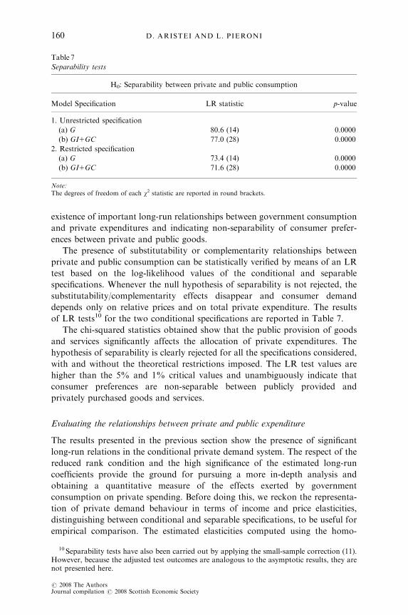
of LR tests10 for the two conditional specifications are reported in Table 7.

The chi-squared statistics obtained show that the public provision of goods

and services significantly affects the allocation of private expenditures. The

hypothesis of separability is clearly rejected for all the specifications considered,

with and without the theoretical restrictions imposed. The LR test values are

higher than the 5% and 1% critical values and unambiguously indicate that

consumer preferences are non-separable between publicly provided and

privately purchased goods and services.

Evaluating the relationships between private and public expenditure

The results presented in the previous section show the presence of significant

long-run relations in the conditional private demand system. The respect of the

reduced rank condition and the high significance of the estimated long-run

coefficients provide the ground for pursuing a more in-depth analysis and

obtaining a quantitative measure of the effects exerted by government

consumption on private spending. Before doing this, we reckon the representa-

tion of private demand behaviour in terms of income and price elasticities,

distinguishing between conditional and separable specifications, to be useful for

empirical comparison. The estimated elasticities computed using the homo-

Table 7

Separability tests

H0: Separability between private and public consumption

Model Specification LR statistic p-value

1. Unrestricted specification

(a) G 80.6 (14) 0.0000

(b) GI1GC 77.0 (28) 0.0000

2. Restricted specification

(a) G 73.4 (14) 0.0000

(b) GI1GC 71.6 (28) 0.0000

Note:The degrees of freedom of each w2 statistic are reported in round brackets.

10 Separability tests have also been carried out by applying the small-sample correction (11).However, because the adjusted test outcomes are analogous to the asymptotic results, they arenot presented here.



geneity and symmetry restricted estimates are presented in Table 8.11 The

significant effects of the I(1) government variables found in the separability tests

lead to a cautious interpretation of the elasticity results of the private demand

system, reported in Section (a) of Table 8. It is worth remarking that the

potential misspecification problems of the separable specification can explain the

unlikely negative value of the income elasticity of ‘Food, Energy and Other non-

durables’,12 while the expected sign and dimension of elasticities are recovered in

the conditional model only (Section (b) of Table 8). As can be noted, the results

seem to be, on the whole, quite plausible: income elasticities at the sample mean

show that ‘Health, education, recreation and culture and social protection’

(‘HER’) are necessary goods. The category ‘Food, Energy and Other non-

durables’ also emerges as a necessary good, with an estimated income elasticity

well below the unity. On the contrary, ‘Services’ are, as expected, luxury goods

with income elasticity 42.

Table 8

Estimated price and income elasticities

Price Elasticities

Income

Elasticities

Marshallian Hicksian

Private expenditures (1) (2) (3) (1) (2) (3)

(a) Separable specification

(1) HER � 1.202 1.156 � 0.802 � 1.135 1.556 � 0.421 0.752

(0.296) (0.649) (0.569) (0.293) (0.607) (0.508) (0.516)

(2) Services 0.110 � 2.728 0.015 0.340 � 1.673 1.333 2.603

(0.136) (0.406) (0.354) (0.132) (0.389) (0.319) (0.315)

(3) Other non-durables � 0.052 1.164 � 0.872 � 0.074 1.066 � 0.993 � 0.239

(0.092) (0.280) (0.334) (0.088) (0.256) (0.304) (0.287)

(b) Conditional to GI and GC

(1) HER � 2.177 2.342 � 1.034 � 2.100 2.693 � 0.596 0.866

(0.349) (0.477) (0.313) (0.351) (0.485) (0.299) (0.262)

(2) Services 0.395 � 2.640 0.051 0.590 � 1.746 1.163 2.192

(0.106) (0.324) (0.285) (0.106) (0.338) (0.285) (0.286)

(3) Other non-durables � 0.110 0.902 � 0.860 � 0.098 0.904 � 0.826 0.068

(0.053) (0.223) (0.227) (0.049) (0.207) (0.204) (0.202)

Note:Asymptotic standard errors in round brackets.

11 Formally, income elasticity and Marshallian and Hicksian price elasticities for theconditional Almost Ideal model (7) are as follows:

Zi ¼ 1þ bi=wi ðIncome ElasticityÞ;eMij ¼ gij=wi þ ð1� ZiÞwj � dij ¼ gij=wi � biwj=wi � dij ðMarshallian Price ElasticityÞ;eHij ¼ gij=wi þ wj � dij ðHicksian Price ElasticityÞ;

where dij is Kronecker’s delta (equal to one if i5 j and zero otherwise).12 These misspecification problems can also affect the results of the cointegration rank test.



The estimated own-price elasticities are all negative and significant at the 5%

level. Moreover, the compensated price elasticity values are always lower than

the uncompensated ones, as implied by the theoretical structure imposed on the

parametric specification. In general, all the estimated price elasticities are well

defined and plausible.

Considering the ‘HER’ and ‘Services’ categories, the own-prices elasticities

show an elastic response, while the presence of food and energy in ‘Other non

durables’ determines an inelastic own-price response. Finally, the statistical

significance of cross-price elasticities in private good demand leads to classify

‘Services’ as substitutes of ‘HER’ and ‘Other non-durables’, while the last two

categories are classified as complementary goods.

Finally, we stress the novelty of the results obtained by both verifying the

assumption of non-separability and taking into account the simultaneous

decomposition of private and public expenditures. This point can be appreciated

by analyzing Table 9, where the estimated elasticities with respect to individual

government expenditure (GI) and collective government expenditure (GC) of

each private expenditure category of the demand system are reported. Firstly,

the results show that private consumption decisions are significantly affected by

the public provision of goods and services and the public sector has

simultaneous crowding-out/in effects on the private sector. Secondly, individual

and collective government expenditures (GI and GC) are more linked with some

private goods and services and less with others. As expected, we note that the

private counterpart of individual government expenditure (‘HER’) is character-

ized by the highest substitutability value. This estimation works against the

claims that the private and public expenditure categories that produce similar

utility cause a crowding-in effect (Kuehlwein, 1998; Fiorito and Kollintzas,

2004). The classical crowding-out hypothesis is confirmed: public expenditure

has a large negative contemporaneous influence on private consumer spending

Table 9

Estimated elasticities with respect to public consumption

Year

HER Services

Other

non-durables Total

GI GC GI GC GI GC GI GC

Sample mean � 0.685 � 0.549 0.369 0.246 � 0.176 � 0.099 � 0.164 � 0.134

(0.263) (0.182) (0.163) (0.109) (0.064) (0.075) (0.058) (0.057)

1970 � 0.605 � 0.560 0.349 0.257 � 0.119 � 0.076 � 0.125 � 0.126

(0.224) (0.184) (0.194) (0.126) (0.046) (0.026) (0.059) (0.050)

1980 � 0.639 � 0.577 0.377 0.276 � 0.163 � 0.101 � 0.143 � 0.134

(0.244) (0.189) (0.207) (0.131) (0.060) (0.033) (0.068) (0.056)

1990 � 0.686 � 0.538 0.353 0.229 � 0.226 � 0.124 � 0.186 � 0.145

(0.263) (0.178) (0.187) (0.103) (0.090) (0.041) (0.061) (0.047)

2000 � 0.668 � 0.470 0.378 0.220 � 0.286 � 0.144 � 0.192 � 0.131

(0.263) (0.158) (0.195) (0.092) (0.110) (0.049) (0.054) (0.053)

Note:Asymptotic standard errors in round brackets.



on health, education, recreation and social protection (the elasticities with

respect to GI and GC, estimated at the sample mean, are equal to � 0.685 and

� 0.549, respectively). Moreover, the elasticities of ‘Other non-durables’ with

respect to government spending are significantly different from zero and

negative (eGIother ¼ �0:176 and eGCother ¼ �0:099), thus indicating, as above, a

substitution relationship between private expenditure and public consumption.

The elasticities of the ‘Services’ category with respect to GI and GC

(eGIservices ¼ 0:369 and eGCservices ¼ 0:246) show that an increase in the public

provision of goods and services causes an increase in private spending due to the

presence of a positive income effect. This strengthens the complementarity effect

exerted by public consumption expenditures and causes a shift of consumer

preferences. This result is in line with the findings of Karras (1994), Kuehlwein

(1998) and Fiorito and Kollintzas (2004) concerning the possibility of having

complementarity relationships between some components of public and private

spending.

From the analysis of the dynamics of the estimated elasticities taken at each

decade, it is possible to note that the elasticity of substitution of the HER

expenditures with respect to GI increases in absolute value (from � 0.605 in

1970 to � 0.668 in 2000) while the impact of GC decreases (from � 0.560 to

� 0.470). Concerning non-durable goods, GI and GC display an upward trend

over the entire sample period, doubling the initial substitutability values. On the

contrary, the elasticity of services with respect to government expenditure shows

a slight downward trend for GC, while the impact of GI remains quite stable

over the sample.

In order to compare our findings with those obtained by the traditional

crowding-out literature, we compute the average effects of GI and GC as a

mean of the elasticities for the three private consumption categories in each

decade.13 A summary of the results is provided in the last two columns of

Table 9. Although the multivariate approach proposed is different from

that adopted in the standard macroeconomic literature, it is worth noting

that the range of estimated elasticities (eGIð1970Þ ¼ �0:125, eGIð2000Þ ¼ �0:192;eGCð1970Þ ¼ �0:126, eGCð2000Þ ¼ �0:131) is very similar to that found in previous

analyses using different estimation procedures, sampling and specifications (see

Darby and Malley, 1996, p. 139), which confirms the validity of our findings.

V Concluding Remarks

In this paper, we have used a micro-based approach to investigate the

relationships between disaggregate private consumption and publicly provided

goods. The different impact of individual and collective government expendi-

tures on private utility function has led to extend the analysis to account for

these heterogeneous behaviours. Thus, a conditional demand system is derived

and government expenditure or its components have been used as a rationed

good. The novelty of our analysis, with respect to the traditional literature,

13 Because each estimated parameter yij is weighted by the budget share, the averagesubstitution elasticities are obtained directly.



concerns the possibility of simultaneously testing for the presence of crowding-

out/in effects in a conditional demand system by verifying the non-separability

hypothesis of individual preferences. To do this, we have assumed that

government expenditure is an exogenous I(1) forcing variable and a conditional

long-run demand system has been specified in a multivariate error correction

model.

Three main empirical implications have been derived by estimating the

conditional long-run demand system for the United Kingdom in the 1964–2002

period. Private consumption decisions are significantly affected by the public

provision of goods and services. Moreover, the decomposition of private

expenditure in three different budget shares leads to simultaneous crowding-out/

in effects. Secondly, we cannot reject the traditional point of view according to

which government expenditure crowds out private goods and services. These

findings are in contrast with recent empirical evidence of complementary effects.

On the other hand, income effects generate a positive impact of government

expenditure on the ‘Services’ category. Thirdly, we have investigated the

coherence of our empirical results with respect to previous works by means of an

aggregate indicator. The average value of public consumption elasticity is found

to be close to the range of previous literature showing the presence of a

significant substitutability relationship.

On the basis of our results, the suggestion is that efficient fiscal policy

planning should take into account the heterogeneous impacts of government

spending on the allocation of private expenditures. The identification of the

interactions between private and public consumption, in fact, not only allows a

better representation of consumer behaviour, but it is also important to improve

the understanding of households’ responsiveness to public welfare programmes.

Thus, further research should be aimed at deepening the analysis of this

interesting topic, by extending the representation of government functional

spending and providing cross-country comparisons.

Acknowledgements

We would like to thank Carlo Andrea Bollino, Federico Perali and all the

participants at the ‘New Developments in Macroeconomic Modelling and

Growth Dynamics’ conference (Faro, 7–9 September 2006) for their useful

comments and suggestions. All the remaining errors are our own.

References

ABAD, A. and QUILIS, E. (2005) Software to perform temporal disaggregation of economic timeseries, Eurostat, Working Papers and Studies.

ASCHAUER, D. (1985). Fiscal policy and aggregate demand. American Economic Review, 75,pp. 117–27.

ASCHAUER, D. (1993). Fiscal policy and aggregate demand: reply. American Economic Review,83, pp. 667–9.

BOSWIJK, H. P. (1994). Testing for an unstable root in conditional and structural errorcorrection models. Journal of Econometrics, 63, pp. 37–60.

BOSWIJK, H. P. (1995). Efficient inference on cointegration parameters in structural errorcorrection models. Journal of Econometrics, 69, pp. 133–58.



BOSWIJK, H. P. and FRANSES, P. (1992). Dynamic specification and cointegration. OxfordBulletin of Economic and Statistics, 54, pp. 369–81.

CHOW, G. and LIN, A. L. (1971). Best linear unbiased interpolation, distribution andextrapolation of time series by related series. The Review of Economics and Statistics, 53,pp. 372–5.

DARBY, J. and MALLEY, J. (1996). Fiscal policy and aggregate consumption: new evidence fromthe United States. Scottish Journal of Political Economy, 43, pp. 129–45.

DEATON, A. S. (1981). Theoretical and empirical approaches to consumer demand underrationing. In A. S. Deaton, Essays in the Theory and Measurement of Consumer Behaviour.Cambridge: Cambridge University Press, pp. 55–72.

DEATON, A. S. and MUELLBAUER, J. (1980). An almost ideal demand system. AmericanEconomic Review, 70, pp. 312–26.

DEATON, A. S. and MUELLBAUER, J. (1981). Functional forms for labour supply andcommodity demands with and without quantity restrictions. Econometrica, 49, pp. 1521–33.

DICKEY, D. A. and FULLER, W. A. (1979). Distribution of estimators for autoregressive timeseries with unit roots. Journal of the American Statistical Association, 74, pp. 427–31.

DUFOUR, J. M. and KHALAF, L. (2002). Simulation based finite and large sample tests inmultivariate regressions. Journal of Econometrics, 111, pp. 303–22.

FERNANDEZ, R. B. (1981). Methodological note on the estimation of time series. Review ofEconomic and Statistics, 63, pp. 471–8.

FIORITO, R. and KOLLINTZAS, T. (2004). Public goods, merit goods, and the relation betweenprivate and government consumption. European Economic Review, 48, pp. 1367–98.

GRAHAM, F. C. (1993). Fiscal policy and aggregate demand: comment. American EconomicReview, 83, pp. 659–66.

GRANGER, C. W. J. and LIN, J. L. (1995). Causality in the long-run. Econometric Theory, 11,pp. 530–6.

HARBO, I., JOHANSEN, S., NIELSEN, B. and RAHBEK, A. (1998). Asymptotic inference oncointegrating rank in partial systems. Journal of Business and Economic Statistics, 16, pp.388–99.

JOHANSEN, S. (1992). Cointegration in partial systems and the efficiency of single-equationanalysis. Journal of Econometrics, 52, pp. 389–402.

JOHANSEN, S. (1995). Identifying restrictions of linear equations with applications tosimultaneous equations and cointegration. Journal of Econometrics, 69, pp. 111–32.

KARRAS, G. (1994). Government spending and private consumption: some internationalevidence. Journal of Money, Credit and Banking, 26, pp. 9–22.

KORMENDI, R. (1983). Government debt, government spending and private sector behaviour.American Economic Review, 73, pp. 994–1010.

KUEHLWEIN, M. (1998). Evidence on the substitutability between government purchases andconsumer spending within specific spending categories. Economics Letters, 58, pp. 325–9.

LAITINEN, K. (1978). Why is demand homogeneity so often rejected? Economics Letters, 1, pp.187–91.

LEVAGGI, R. (1998). The effects of the provision of public goods on private consumption inItaly: a macroeconomic perspective. International Review of Economics and Business, 45,pp. 47–63.

LEVAGGI, R. (1999). Does government expenditure crowd out private consumption in Italy?Evidence from a microeconomic model. International Review of Applied Economics, 13, pp.241–51.

LEWBEL, A. and NG, S. (2005). Demand systems with nonstationary prices. Review ofEconomics and Statistics, 87, pp. 479–94.

LITTERMAN, R. B. (1983). A random walk, markov model for the distribution of time series.Journal of Business and Economic Statistics, 1, pp. 169–73.

MACKINNON, J. G. (1996). Numerical distribution functions for unit root and cointegrationtests. Journal of Applied Econometrics, 11, pp. 601–18.

MARRINAN, J. (1998). Government consumption and private consumption correlations. Journalof International Money and Finance, 17, pp. 615–36.

NEARY, J. P. and ROBERTS, K. W. S. (1980). The theory of household behaviour underrationing. American Economic Review, 13, pp. 25–42.

NG, S. (1995). Testing for homogeneity in demand systems when the regressors arenonstationary. Journal of Applied Econometrics, 10, pp. 147–63.



NI, S. (1995). An empirical analysis on the substitutability between private consumption andgovernment purchases. Journal of Monetary Economics, 36, pp. 593–605.

OFFICE FOR NATIONAL STATISTICS (various years). United Kingdom National Accounts – TheBlue Book.

PESARAN, M. H. and SHIN, Y. (2002). Long-run structural modelling. Econometrics Reviews,21, pp. 49–87.

PESARAN, M. H., SHIN, Y. and SMITH, R. J. (2000). Structural analysis of vector errorcorrection models with exogenous I(1) variables. Journal of Econometrics, 97, pp. 293–343.

PHILLIPS, P. C. B. and PERRON, P. (1988). Testing for a unit root in time series regression.Biometrika, 75, pp. 335–46.

PIERONI, L. and ARISTEI, D. (2005). Testing separability of public consumption in householddecisions. International Review of Applied Economics, 19, pp. 198–218.

POLLAK, R. A. (1969). Conditional demand functions and consumption theory. The QuarterlyJournal of Economics, 83, pp. 60–78.

POLLAK, R. A. (1971). Conditional demand functions and the implication of separable utility.Southern Economic Journal, 78, pp. 401–14.

PUDNEY, S. E. (1981). An empirical method of approximating the separable structure ofconsumer preferences. Review of Economic Studies, 48, pp. 561–77.

REIMERS, H. (1992). Comparison of multivariate cointegration tests. Statistical Papers, 33, pp.335–59.

SANTOS SILVA, J. M. C. and CARDOSO, F. N. (2001). The Chow-Lin method using dynamicmodels. Economic Modelling, 18, pp. 269–80.

STURM, J. E. (1998). Public Capital Expenditure in OECD Countries: The Causes and Impact ofthe Decline in Public Capital Spending. Cheltenham: Edward Elgar.

THEIL, H. and FIEBIG, D. G. (1985). Small sample and large equation systems. In E. J. Hannan,P. R. Krishnaiah and M. M. Rao (eds), Handbook of Statistics 5: Time Series in the TimeDomain. Amsterdam: North-Holland, pp. 451–80.

TRIDIMAS, G. (2002). The dependence of private consumer demand on public consumptionexpenditures. Theory and evidence. Public Finance Review, 30, pp. 251–72.

URBAIN, J. P. (1995). Partial versus full system modelling of cointegrated systems: an empiricalillustration. Journal of Econometrics, 69, pp. 177–210.

Date of receipt of final manuscript: 10 May 2007



GOVERNMENT CONSUMPTION AND THE COMPOSITION OF PRIVATE EXPENDITURE: A CONDITIONAL ERROR CORRECTION...

Documents

Transcript of GOVERNMENT CONSUMPTION AND THE COMPOSITION OF PRIVATE EXPENDITURE: A CONDITIONAL ERROR CORRECTION...