�����������������

Citation: Zhang, D.; Yu, Z.; Xu, Y.;

Ding, L.; Ding, H.; Yu, Q.; Su, Z.

GNSS Aided Long-Range 3D

Displacement Sensing for High-Rise

Structures with Two Non-Overlapping

Cameras. Remote Sens. 2022, 14, 379.

https://doi.org/10.3390/rs14020379

Academic Editors: Anna Visvizi,

Wadee Alhalabi, Shahira Assem

Abdel Razek, Paolo Gerli and

Orlando Troisi

Received: 6 December 2021

Accepted: 13 January 2022

Published: 14 January 2022

Publisher’s Note: MDPI stays neutral

with regard to jurisdictional claims in

published maps and institutional affil-

iations.

Copyright: © 2022 by the authors.

Licensee MDPI, Basel, Switzerland.

This article is an open access article

distributed under the terms and

conditions of the Creative Commons

Attribution (CC BY) license (https://

creativecommons.org/licenses/by/

4.0/).

remote sensing

Technical Note

GNSS Aided Long-Range 3D Displacement Sensing forHigh-Rise Structures with Two Non-Overlapping CamerasDongsheng Zhang 1,2 , Zhenyang Yu 1, Yan Xu 3, Li Ding 1,2, Hu Ding 1,2 , Qifeng Yu 4 and Zhilong Su 1,2,*

1 Shanghai Key Laboratory of Mechanics in Energy Engineering, Shanghai Institute of Applied Mathematicsand Mechanics, School of Mechanics and Engineering Science, Shanghai University, Shanghai 200444, China;donzhang@staff.shu.edu.cn (D.Z.); Zhenyang_Yu@shu.edu.cn (Z.Y.); liding@oa.shu.edu.cn (L.D.);dinghu3@shu.edu.cn (H.D.)

2 National Demonstration Center for Experimental Mechanics Education, Shanghai University,Shanghai 200444, China

3 School of Materials and Chemistry, University of Shanghai for Science and Technology,Shanghai 200093, China; 1935040112@st.usst.edu.cn

4 College of Aerospace Science and Engineering, National University of Defense Technology,Changsha 410073, China; yuqifeng@nudt.edu.cn

* Correspondence: zhilong8845@shu.edu.cn

Abstract: Image-based displacement measurement techniques are widely used for sensing thedeformation of structures, and plays an increasing role in structural health monitoring owing to itsbenefit of non-contacting. In this study, a non-overlapping dual camera measurement model withthe aid of global navigation satellite system (GNSS) is proposed to sense the three-dimensional (3D)displacements of high-rise structures. Each component of the dual camera system can measure a pairof displacement components of a target point in a 3D space, and its pose relative to the target can beobtained by combining a built-in inclinometer and a GNSS system. To eliminate the coupling of lateraland vertical displacements caused by the perspective projection, a homography-based transformationis introduced to correct the inclined image planes. In contrast to the stereo vision-based displacementmeasurement techniques, the proposed method does not require the overlapping of the field ofviews and the calibration of the vision geometry. Both simulation and experiment demonstrate thefeasibility and correctness of the proposed method, heralding that it has a potential capacity in thefield of remote health monitoring for high-rise buildings.

Keywords: video-image measurement; 3D displacement sensing; structural health monitoring;high-rise buildings

1. Introduction

With the rapid development of the global economy and construction technology, theconstruction of high-rise structures, such as civil buildings, industrial chimneys and towers,has maintained a rapid growth over the past ten years [1]. However, these structuresmay fail due to long-term load, environmental changes, and other factors [2,3]. Thehorizontal deformations, including shearing displacement between stories and overallbending, caused by wind, are the dominant factors for health monitoring [4,5]. Meanwhile,the overall vertical displacement of a high-rise structure is also a critical indicator to reflectthe structural behavior in the service period [6]. Therefore, monitoring the 3D displacementsof high-rise structures is of great significance for inspecting structural reliability and safetyin structural health monitoring (SHM).

Traditionally, it is common to use the contact sensors for monitoring the lateral dis-placement of high-rise buildings [7]. Among them, displacement meters and accelerometersare two types that are mostly used. e.g., accelerometers can effectively capture the accel-eration and further allow for deriving the displacement in a specific coordinate direction

Remote Sens. 2022, 14, 379. https://doi.org/10.3390/rs14020379 https://www.mdpi.com/journal/remotesensing

Remote Sens. 2022, 14, 379 2 of 16

of large facilities under external excitation [8–10]. Due to the development of the globalnavigation satellite system (GNSS), it is widely used to monitor the lateral and vertical dis-placement of high-rise buildings and bridges, owing to its small dependence on the serviceenvironment [11–14]. Authors in [15] have attempted to sense the lateral displacement ofthe high-rise buildings subjected to wind load by installing an inclinometer at a target pointon the buildings, and remotely cooperating with a remote sensing vibration detector. Evensome sensors fabricated by new materials have also been used for high-rise building healthmonitoring, such as the PZT piezoelectric ceramics [16] and nanometer material [17].

Although most of the SHM systems are well-established, being based on these sensorsafter decades of development, they are working based on the data collection in the mannerof point-contact sensing. Aside from the hassles in maintenance, this raises another issue:that it is difficult and expensive to collect the 3D deformation of multiple points simulta-neously since it requires the integration of multiple sensors in the structures. To solve theproblems, several non-contact measurement techniques have been established to performhealth monitoring of structures, such as the laser displacement meters and the phase-scanned radars, which have been applied to collect the deformation data of bridges, dams,and high-rise buildings [18–21]. Although these systems can monitor the displacementof large infrastructures without installing sensors on the structures, it is difficult for themto achieve long-term stable monitoring because of their dependence on stable referencepoints [11]. Image-based displacement measurement techniques have significantly alteredthe progress of health monitoring large infrastructures due to the advantages of long dis-tance, non-contact, high accuracy, and multi-point or full-field measurement [22]. A widelyused image-based technique is derived from stereo vision [23,24], which is capable of re-trieving the 3D displacement of targets, such as masonry structures [25,26], bridges [27,28],and even underwater structures [29]. As a result of stereo vision, a good calibration ofthe 3D imaging system is critical for obtaining accurate measurements. However, it ischallenging for long range sensing due to the large field of view and complex measurementenvironment. Some alternate techniques are accordingly developed for easy remote moni-toring. A monocular video deflectometer (MVD) is such a promising technique. Two typesof MVDs were reported to measure the deflection of the bridges based on digital imagecorrelation (DIC) [8,30]. Although both are effective in conditions with oblique optical axis,the latter advanced the MVD by considering the variation of the pitch angles in the wholeimage. In addition, the motion amplification method based on the monocular video wasalso a promising method for the monitoring of structures [31].

For image based SHM of high-rise buildings, several related studies are acknowledged.Jong et al. divided a high-rise building into sections and then measured the lateral defor-mation by accumulating the relative displacement of adjacent sections [32]. However, theydid not consider the accumulation error of the relative displacement. Guo et al. proposeda stratification method based on projective rectification, with lines to monitor the seismicdisplacement of buildings [33]. Although the method is effective in reducing the influenceof camera motion, it highly relies on the line features which might be unavailable in somesituations. Recently, Ye et al. reported to monitor, long-term, the displacement of an ancienttower caused by the change of geotechnical conditions with a dual camera system [34];the work shows the advantages of image-based SHM for high-rise buildings, yet does notconsider the error induced by yaw angle variation. Besides, other researchers have alsoattempted to combine the GNSS with the image-based methods for sensing the deforma-tion of the large-scale structures from a long distance [35]. These recent progresses arepromoting the development of the SHM techniques and inspiring the related communitiesto build new methods.

This study proposes a non-overlapping dual camera model for sensing the 3D dis-placement of high-rise buildings from a long-range by combining image tracking with theGNSS system and inclinometers. The proposed method is described in detail by followingthe organization as: Section 2 introduces the methodology, including the non-overlappingdual camera measurement model in Section 2.1 and the principle of GNSS-aided yaw angle

Remote Sens. 2022, 14, 379 3 of 16

determination in Section 2.2; Section 3 shows the simulation and experimental results;Section 4 discusses the influence of the positioning accuracy of GNSS on the yaw angle,and Section 5 concludes.

2. Methodology

As towering structures are mainly subjected to random wind load, the lateral dis-placement is a critical control indicator for structural safety assessment. In addition, thevertical response may be remarkable even if the wind load is horizontal, implying that thevertical displacement or settlement should be concern also. However, most of the high-risestructures are located in the built-up yet prosperous urban areas, so it is difficult to find anappropriate workspace for setting up a stereo vision system (such as 3D-DIC) with goodoptical geometry to sense the lateral and vertical displacements of the structure’s sections ofinterest. To address this predicament, this section elaborates on a 3D displacement remotesensing system that does not relies on stereo vision geometry. The proposed system canmeasure the 3D displacement of a towering structure with two non-overlapping camerasplaced at different sides of the structure. Details are described as follows.

2.1. Three-Dimensional Displacement Sensing with Two Non-Overlapping Cameras

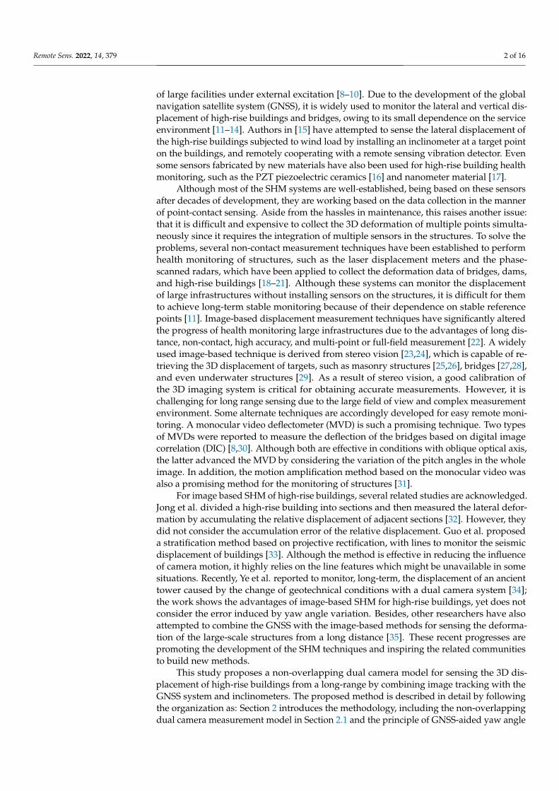
Generally, the lateral and vertical displacements characterize the overall deforma-tion at a certain floor relative to the ground reference for high-rise structures, and theintraformational displacement of the floors is a low-order quantity compared to the overalldisplacement. Hence, it is reasonable to simplify the target floor to be measured to a pointin 3D space. With this assumption, measuring the lateral and vertical displacements of astructure’s floor is turned into a problem of measuring 3D displacements of a space pointfrom two non-overlapping views, as illustrated in Figure 1.

Remote Sens. 2022, 14, x FOR PEER REVIEW 3 of 16

GNSS system and inclinometers. The proposed method is described in detail by following the organization as: Section 2 introduces the methodology, including the non-overlapping dual camera measurement model in Section 2.1 and the principle of GNSS-aided yaw an-gle determination in Section 2.2; Section 3 shows the simulation and experimental results; Section 4 discusses the influence of the positioning accuracy of GNSS on the yaw angle, and Section 5 concludes.

2. Methodology As towering structures are mainly subjected to random wind load, the lateral dis-

placement is a critical control indicator for structural safety assessment. In addition, the vertical response may be remarkable even if the wind load is horizontal, implying that the vertical displacement or settlement should be concern also. However, most of the high-rise structures are located in the built-up yet prosperous urban areas, so it is difficult to find an appropriate workspace for setting up a stereo vision system (such as 3D-DIC) with good optical geometry to sense the lateral and vertical displacements of the structure’s sections of interest. To address this predicament, this section elaborates on a 3D displace-ment remote sensing system that does not relies on stereo vision geometry. The proposed system can measure the 3D displacement of a towering structure with two non-overlap-ping cameras placed at different sides of the structure. Details are described as follows.

2.1. Three-Dimensional Displacement Sensing with Two Non-Overlapping Cameras Generally, the lateral and vertical displacements characterize the overall deformation

at a certain floor relative to the ground reference for high-rise structures, and the intra-formational displacement of the floors is a low-order quantity compared to the overall displacement. Hence, it is reasonable to simplify the target floor to be measured to a point in 3D space. With this assumption, measuring the lateral and vertical displacements of a structure’s floor is turned into a problem of measuring 3D displacements of a space point from two non-overlapping views, as illustrated in Figure 1.

Figure 1. 3D displacement sensing with two non-overlapping cameras C1 and C2.

As shown in Figure 1, the different target floors of the high-rise building are observed by the cameras C1 and C2 from its left and front sides, respectively, obviously forming two

Figure 1. 3D displacement sensing with two non-overlapping cameras C1 and C2.

As shown in Figure 1, the different target floors of the high-rise building are observedby the cameras C1 and C2 from its left and front sides, respectively, obviously formingtwo non-overlapping views. The lines of sight of the cameras strike different sides ofthe target floors, generating a set of target points, e.g., T1 to T6. For any pair of targetpoints, such as Ti (i = 1, 2) on the top floor, the corresponding cameras can sense thedisplacement components, denoted by Vi and Ui, parallel to their image planes. If we

Remote Sens. 2022, 14, 379 4 of 16

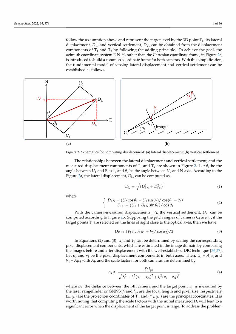
follow the assumption above and represent the target level by the 3D point Te, its lateraldisplacement, DL, and vertical settlement, DV, can be obtained from the displacementcomponents of T1 and T2 by following the adding principle. To achieve the goal, theazimuth coordinate system E-N-H, rather than the Cartesian coordinate frame, in Figure 2a,is introduced to build a common coordinate frame for both cameras. With this simplification,the fundamental model of sensing lateral displacement and vertical settlement can beestablished as follows.

Remote Sens. 2022, 14, x FOR PEER REVIEW 4 of 16

non-overlapping views. The lines of sight of the cameras strike different sides of the target floors, generating a set of target points, e.g., T1 to T6. For any pair of target points, such as Ti (i = 1, 2) on the top floor, the corresponding cameras can sense the displacement com-ponents, denoted by Vi and Ui, parallel to their image planes. If we follow the assumption above and represent the target level by the 3D point T , its lateral displacement, DL, and vertical settlement, DV, can be obtained from the displacement components of T1 and T2 by following the adding principle. To achieve the goal, the azimuth coordinate system E-N-H, rather than the Cartesian coordinate frame, in Figure 2a, is introduced to build a common coordinate frame for both cameras. With this simplification, the fundamental model of sensing lateral displacement and vertical settlement can be established as fol-lows.

(a) (b)

Figure 2. Schematics for computing displacement: (a) lateral displacement; (b) vertical settlement.

The relationships between the lateral displacement and vertical settlement, and the measured displacement components of T and T are shown in Figure 2. Let θ1 be the an-gle between U1 and E-axis, and θ2 be the angle between U2 and N-axis. According to the Figure 2a, the lateral displacement, DL, can be computed as:

2 2L LN LE( )D D D= + (1)

where

LN 2 1 1 2 1 2

LE 1 LN 1 1

( cos sin ) / cos( - )( sin ) / cos

U UU

= θ − θ θ θ = + θ θ

DD D

(2)

With the camera-measured displacements, Vi, the vertical settlement, Dv, can be com-puted according to Figure 2b. Supposing the pitch angles of cameras Ci are αi, if the target points Ti are selected on the lines of sight close to the optical axes, then we have

V 1 1 2 2cos )c( /o 2sD V V≈ +α α/ / (3)

In Equations (2) and (3), Ui and Vi can be determined by scaling the corresponding pixel displacement components, which are estimated in the image domain by comparing the images before and after displacement with the well-established DIC technique [36,37]. Let ui and vi be the pixel displacement components in both axes. Then, Ui = Aiui and Vi = Aivi with Ai, and the scale factors for both cameras are determined by

≈+ − + −2 2 2 2 2( ) ( )

i psi

i i ci i cii i

D lA

f l x x l y y (4)

Figure 2. Schematics for computing displacement: (a) lateral displacement; (b) vertical settlement.

The relationships between the lateral displacement and vertical settlement, and themeasured displacement components of T1 and T2 are shown in Figure 2. Let θ1 be theangle between U1 and E-axis, and θ2 be the angle between U2 and N-axis. According to theFigure 2a, the lateral displacement, DL, can be computed as:

DL =√(D2

LN + D2LE) (1)

where {DLN = (U2 cos θ1 −U1 sin θ2)/ cos(θ1 − θ2)

DLE = (U1 + DLN sin θ1)/ cos θ1(2)

With the camera-measured displacements, Vi, the vertical settlement, Dv, can becomputed according to Figure 2b. Supposing the pitch angles of cameras Ci are αi, if thetarget points Ti are selected on the lines of sight close to the optical axes, then we have

DV ≈ (V1/ cos α1 + V2/ cos α2)/2 (3)

In Equations (2) and (3), Ui and Vi can be determined by scaling the correspondingpixel displacement components, which are estimated in the image domain by comparingthe images before and after displacement with the well-established DIC technique [36,37].Let ui and vi be the pixel displacement components in both axes. Then, Ui = Aiui andVi = Aivi with Ai, and the scale factors for both cameras are determined by

Ai ≈Dilps√

fi2 + li

2(xi − xci)2 + li

2(yi − yci)2

(4)

where Di, the distance between the i-th camera and the target point Ti, is measured bythe laser rangefinder or GNNS. fi and lps are the focal length and pixel size, respectively,(xi, yi) are the projection coordinates of Ti, and (xci, yci) are the principal coordinates. It isworth noting that computing the scale factors with the initial measured Di will lead to asignificant error when the displacement of the target point is large. To address the problem,

Remote Sens. 2022, 14, 379 5 of 16

we recommend computing the current scale factors by updating the distances Di with theinitially estimated displacement components, DLE and DLN. The updated distances, Di

*,related to the current position of the target Ti, are given by Equation (5). The current scalefactors are then computed by replacing the initial distances, Di, in Equation (4) with theupdated distances Di

*.

Di∗ =

√(Di sin αi + DV)

2 + (Di cos αi cos θi + DLN)2 + (Di cos αi sin θi + DLE)

2 (5)

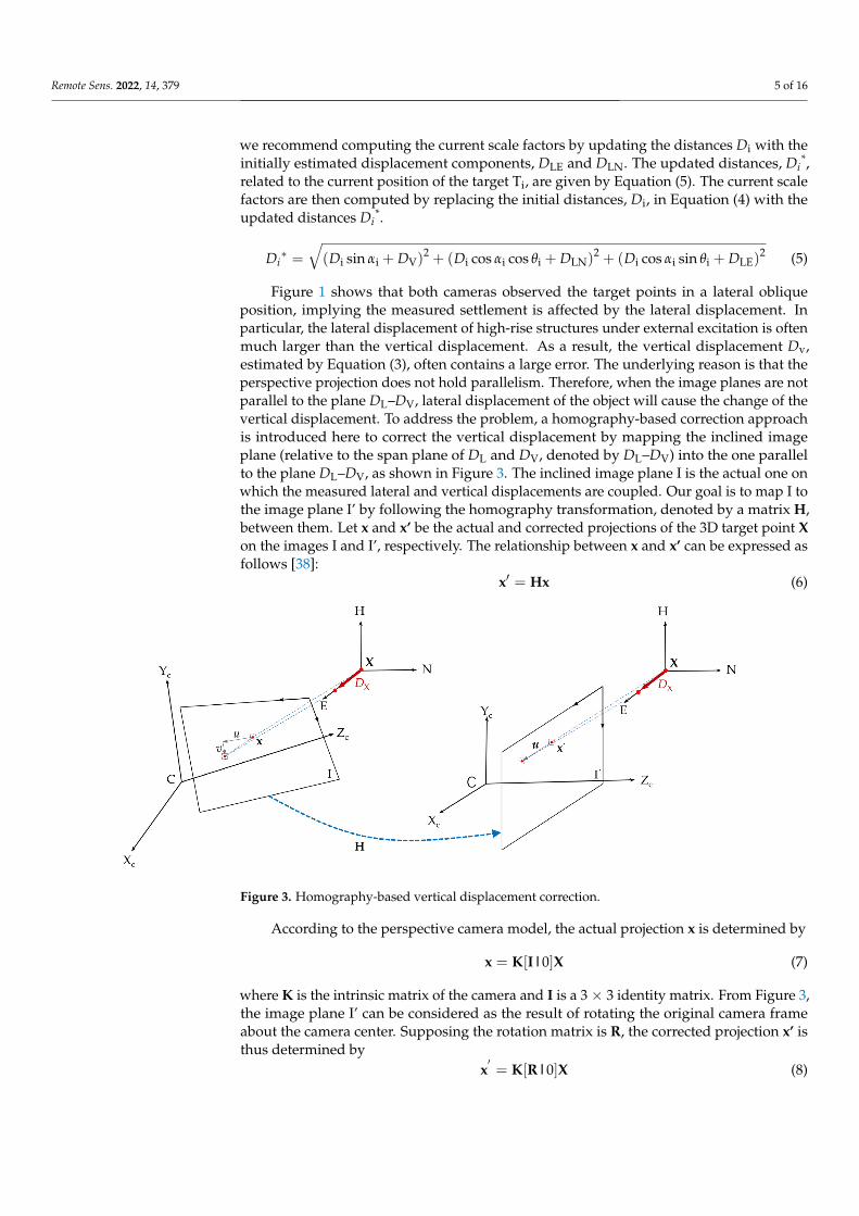
Figure 1 shows that both cameras observed the target points in a lateral obliqueposition, implying the measured settlement is affected by the lateral displacement. Inparticular, the lateral displacement of high-rise structures under external excitation is oftenmuch larger than the vertical displacement. As a result, the vertical displacement Dv,estimated by Equation (3), often contains a large error. The underlying reason is that theperspective projection does not hold parallelism. Therefore, when the image planes are notparallel to the plane DL–DV, lateral displacement of the object will cause the change of thevertical displacement. To address the problem, a homography-based correction approachis introduced here to correct the vertical displacement by mapping the inclined imageplane (relative to the span plane of DL and DV, denoted by DL–DV) into the one parallelto the plane DL–DV, as shown in Figure 3. The inclined image plane I is the actual one onwhich the measured lateral and vertical displacements are coupled. Our goal is to map I tothe image plane I’ by following the homography transformation, denoted by a matrix H,between them. Let x and x’ be the actual and corrected projections of the 3D target point Xon the images I and I’, respectively. The relationship between x and x’ can be expressed asfollows [38]:

x′ = Hx (6)

Remote Sens. 2022, 14, x FOR PEER REVIEW 5 of 16

where Di, the distance between the i-th camera and the target point Ti, is measured by the laser rangefinder or GNNS. fi and lps are the focal length and pixel size, respectively, (xi, yi) are the projection coordinates of Ti, and (xci, yci) are the principal coordinates. It is worth noting that computing the scale factors with the initial measured Di will lead to a signifi-cant error when the displacement of the target point is large. To address the problem, we recommend computing the current scale factors by updating the distances Di with the initially estimated displacement components, DLE and DLN. The updated distances, Di*, related to the current position of the target Ti, are given by Equation (5). The current scale factors are then computed by replacing the initial distances, Di, in Equation (4) with the updated distances Di*.

α α α= + + θ + + θ +2 2 2i V i i LN i i

*LE( sin ) ( cos cos ) ( cos sin )i i i iD D D D D D D (5)

Figure 1 shows that both cameras observed the target points in a lateral oblique po-sition, implying the measured settlement is affected by the lateral displacement. In partic-ular, the lateral displacement of high-rise structures under external excitation is often much larger than the vertical displacement. As a result, the vertical displacement Dv, esti-mated by Equation (3), often contains a large error. The underlying reason is that the per-spective projection does not hold parallelism. Therefore, when the image planes are not parallel to the plane DL–DV, lateral displacement of the object will cause the change of the vertical displacement. To address the problem, a homography-based correction approach is introduced here to correct the vertical displacement by mapping the inclined image plane (relative to the span plane of DL and DV, denoted by DL–DV) into the one parallel to the plane DL–DV, as shown in Figure 3. The inclined image plane I is the actual one on which the measured lateral and vertical displacements are coupled. Our goal is to map I to the image plane I’ by following the homography transformation, denoted by a matrix H, between them. Let x and x’ be the actual and corrected projections of the 3D target point X on the images I and I’, respectively. The relationship between x and x’ can be expressed as follows [38]:

′ = Hxx (6)

Figure 3. Homography-based vertical displacement correction.

According to the perspective camera model, the actual projection x is determined by

= x K[I|0]X (7)

where K is the intrinsic matrix of the camera and I is a 3 × 3 identity matrix. From Figure 3, the image plane I’ can be considered as the result of rotating the original camera frame

Figure 3. Homography-based vertical displacement correction.

According to the perspective camera model, the actual projection x is determined by

x = K[I|0]X (7)

where K is the intrinsic matrix of the camera and I is a 3 × 3 identity matrix. From Figure 3,the image plane I’ can be considered as the result of rotating the original camera frameabout the camera center. Supposing the rotation matrix is R, the corrected projection x’ isthus determined by

x′= K[R|0]X (8)

Remote Sens. 2022, 14, 379 6 of 16

Eliminating X by combining Equations (7) and (8) shows that x’ = KRK−1x. Accordingto Equation (6), the homography matrix H can be determined as:

H = KRK−1 (9)

This implies that, for a calibrated camera, the true vertical displacement of the targetcan be retrieved by estimating the corrected projection x’ via Equations (6) and (9), wherethe rotation matrix R can be computed according to each camera pose, measured in theazimuth frame E-N-H and the displacement direction of the equivalent target point. Forcamera Ci, its pose consists of the pitch angle αi, roll angle and yaw angle θi. The formertwo angles are measured by following the methods in [29,31], while measuring the latterone is not trivial in long-range high-rise structure displacement sensing, which will beintroduced in the next section.

2.2. Determining the Yaw Angles of the Cameras with GNSS

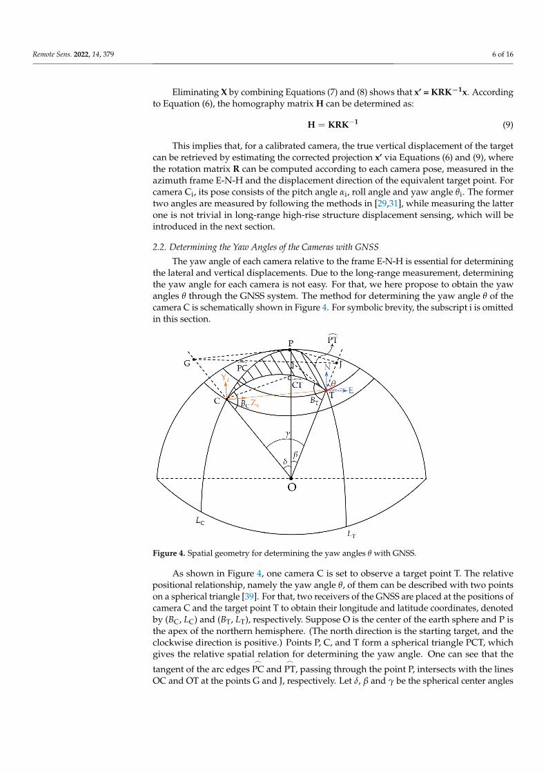
The yaw angle of each camera relative to the frame E-N-H is essential for determiningthe lateral and vertical displacements. Due to the long-range measurement, determiningthe yaw angle for each camera is not easy. For that, we here propose to obtain the yawangles θ through the GNSS system. The method for determining the yaw angle θ of thecamera C is schematically shown in Figure 4. For symbolic brevity, the subscript i is omittedin this section.

Remote Sens. 2022, 14, x FOR PEER REVIEW 6 of 16

about the camera center. Supposing the rotation matrix is R, the corrected projection x’ is thus determined by

′ =x K[R|0]X (8)

Eliminating X by combining Equations (7) and (8) shows that x’ = KRK−1x. According to Equation (6), the homography matrix H can be determined as:

= -1H KRK (9)

This implies that, for a calibrated camera, the true vertical displacement of the target can be retrieved by estimating the corrected projection x’ via Equations (6) and (9), where the rotation matrix R can be computed according to each camera pose, measured in the azimuth frame E-N-H and the displacement direction of the equivalent target point. For camera Ci, its pose consists of the pitch angle αi, roll angle and yaw angle θi. The former two angles are measured by following the methods in [29,31], while measuring the latter one is not trivial in long-range high-rise structure displacement sensing, which will be introduced in the next section.

2.2. Determining the Yaw Angles of the Cameras with GNSS The yaw angle of each camera relative to the frame E-N-H is essential for determining

the lateral and vertical displacements. Due to the long-range measurement, determining the yaw angle for each camera is not easy. For that, we here propose to obtain the yaw angles θ through the GNSS system. The method for determining the yaw angle θ of the camera C is schematically shown in Figure 4. For symbolic brevity, the subscript i is omit-ted in this section.

Figure 4. Spatial geometry for determining the yaw angles θ with GNSS.

As shown in Figure 4, one camera C is set to observe a target point T. The relative positional relationship, namely the yaw angle θ, of them can be described with two points on a spherical triangle [39]. For that, two receivers of the GNSS are placed at the positions of camera C and the target point T to obtain their longitude and latitude coordinates, de-noted by (BC, LC) and (BT, LT), respectively. Suppose O is the center of the earth sphere and P is the apex of the northern hemisphere. (The north direction is the starting target, and the clockwise direction is positive.) Points P, C, and T form a spherical triangle PCT, which

Figure 4. Spatial geometry for determining the yaw angles θ with GNSS.

As shown in Figure 4, one camera C is set to observe a target point T. The relativepositional relationship, namely the yaw angle θ, of them can be described with two pointson a spherical triangle [39]. For that, two receivers of the GNSS are placed at the positions ofcamera C and the target point T to obtain their longitude and latitude coordinates, denotedby (BC, LC) and (BT, LT), respectively. Suppose O is the center of the earth sphere and P isthe apex of the northern hemisphere. (The north direction is the starting target, and theclockwise direction is positive.) Points P, C, and T form a spherical triangle PCT, whichgives the relative spatial relation for determining the yaw angle. One can see that the

tangent of the arc edges_

PC and_PT, passing through the point P, intersects with the lines

OC and OT at the points G and J, respectively. Let δ, β and γ be the spherical center angles

Remote Sens. 2022, 14, 379 7 of 16

corresponding to the arc edges_

PC,_PT and

_CT, respectively. We can obtain the following

relationship according to the cosine formula of the spherical triangle:

γ = arccos(cos δ cos β + sin δ sin β cos∠P) (10)

where ∠P = LC–LT is the dihedral angle between planes COP and TOP, δ = 90◦ − BC, andβ = 90◦ − BT.

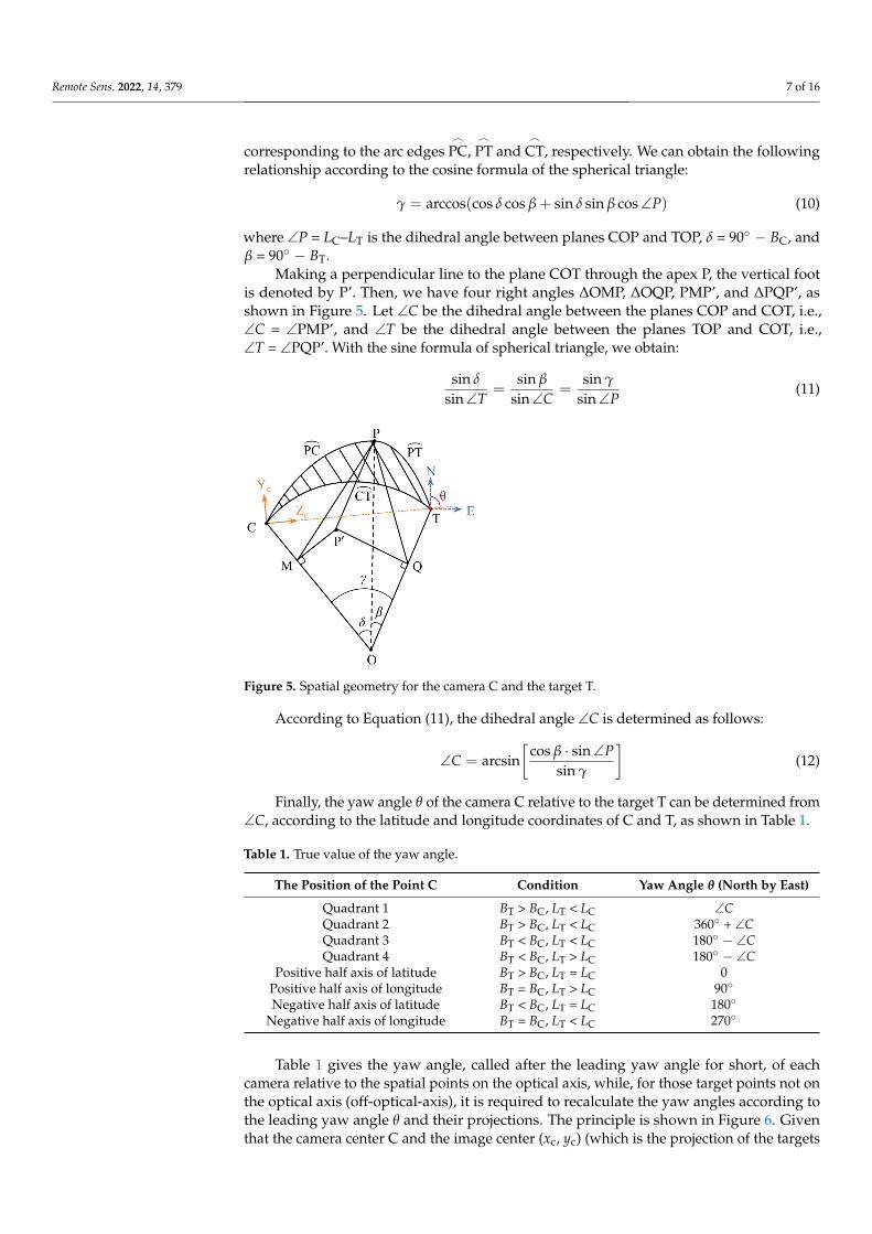
Making a perpendicular line to the plane COT through the apex P, the vertical footis denoted by P’. Then, we have four right angles ∆OMP, ∆OQP, PMP’, and ∆PQP’, asshown in Figure 5. Let ∠C be the dihedral angle between the planes COP and COT, i.e.,∠C = ∠PMP’, and ∠T be the dihedral angle between the planes TOP and COT, i.e.,∠T = ∠PQP’. With the sine formula of spherical triangle, we obtain:

sin δ

sin∠T=

sin β

sin∠C=

sin γ

sin∠P(11)

Remote Sens. 2022, 14, x FOR PEER REVIEW 7 of 16

gives the relative spatial relation for determining the yaw angle. One can see that the tan-gent of the arc edges ⁀PC and ⁀PT, passing through the point P, intersects with the lines OC and OT at the points G and J, respectively. Let δ, β and γ be the spherical center angles corresponding to the arc edges ⁀PC, ⁀PT and ⁀CT, respectively. We can obtain the following relationship according to the cosine formula of the spherical triangle:

arccos(cos cos sin sin cos )P= + ∠γ δ β βδ (10)

where ∠P = LC–LT is the dihedral angle between planes COP and TOP, δ = 90°−BC, and β = 90°−BT.

Making a perpendicular line to the plane COT through the apex P, the vertical foot is denoted by P’. Then, we have four right angles ΔOMP, ΔOQP, PMP’, and ΔPQP’, as shown in Figure 5. Let ∠C be the dihedral angle between the planes COP and COT, i.e., ∠C = ∠PMP’, and ∠T be the dihedral angle between the planes TOP and COT, i.e., ∠T = ∠PQP’. With the sine formula of spherical triangle, we obtain:

sin sin sinsin sin sinT C P

= =∠ ∠ ∠δ β γ (11)

Figure 5. Spatial geometry for the camera C and the target T.

According to Equation (11), the dihedral angle ∠C is determined as follows:

cos sin = arcsinsin

PC ⋅ ∠∠

βγ

(12)

Finally, the yaw angle θ of the camera C relative to the target T can be determined from ∠C, according to the latitude and longitude coordinates of C and T, as shown in Table 1.

Table 1. True value of the yaw angle.

The Position of the Point C Condition Yaw Angle θ (North by East) Quadrant 1 BT > BC, LT < LC ∠C Quadrant 2 BT > BC, LT < LC 360° + ∠C Quadrant 3 BT < BC, LT < LC 180° − ∠C Quadrant 4 BT < BC, LT > LC 180° − ∠C

Positive half axis of latitude BT > BC, LT = LC 0 Positive half axis of longitude BT = BC, LT > LC 90° Negative half axis of latitude BT < BC, LT = LC 180°

Negative half axis of longitude BT = BC, LT < LC 270°

Figure 5. Spatial geometry for the camera C and the target T.

According to Equation (11), the dihedral angle ∠C is determined as follows:

∠C = arcsin[

cos β · sin∠Psin γ

](12)

Finally, the yaw angle θ of the camera C relative to the target T can be determined from∠C, according to the latitude and longitude coordinates of C and T, as shown in Table 1.

Table 1. True value of the yaw angle.

The Position of the Point C Condition Yaw Angle θ (North by East)

Quadrant 1 BT > BC, LT < LC ∠CQuadrant 2 BT > BC, LT < LC 360◦ + ∠CQuadrant 3 BT < BC, LT < LC 180◦ − ∠CQuadrant 4 BT < BC, LT > LC 180◦ − ∠C

Positive half axis of latitude BT > BC, LT = LC 0Positive half axis of longitude BT = BC, LT > LC 90◦

Negative half axis of latitude BT < BC, LT = LC 180◦

Negative half axis of longitude BT = BC, LT < LC 270◦

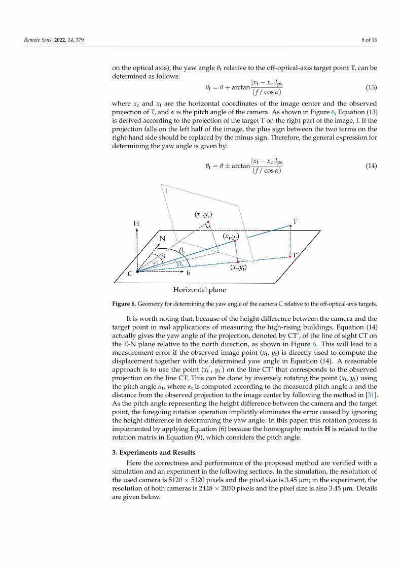
Table 1 gives the yaw angle, called after the leading yaw angle for short, of eachcamera relative to the spatial points on the optical axis, while, for those target points not onthe optical axis (off-optical-axis), it is required to recalculate the yaw angles according tothe leading yaw angle θ and their projections. The principle is shown in Figure 6. Giventhat the camera center C and the image center (xc, yc) (which is the projection of the targets

Remote Sens. 2022, 14, 379 8 of 16

on the optical axis), the yaw angle θt relative to the off-optical-axis target point T, can bedetermined as follows:

θt = θ + arctan|xt − xc|lps

( f / cos α)(13)

where xc and xt are the horizontal coordinates of the image center and the observedprojection of T, and α is the pitch angle of the camera. As shown in Figure 6, Equation (13)is derived according to the projection of the target T on the right part of the image, I. If theprojection falls on the left half of the image, the plus sign between the two terms on theright-hand side should be replaced by the minus sign. Therefore, the general expression fordetermining the yaw angle is given by:

θt = θ ± arctan|xt − xc|lps

( f / cos α)(14)

Remote Sens. 2022, 14, x FOR PEER REVIEW 8 of 16

Table 1 gives the yaw angle, called after the leading yaw angle for short, of each cam-era relative to the spatial points on the optical axis, while, for those target points not on the optical axis (off-optical-axis), it is required to recalculate the yaw angles according to the leading yaw angle θ and their projections. The principle is shown in Figure 6. Given that the camera center C and the image center (xc, yc) (which is the projection of the targets on the optical axis), the yaw angle θt relative to the off-optical-axis target point T, can be determined as follows:

t c pst arctan

( / cos )x x lf

−= +θ θ

α (13)

where xc and xt are the horizontal coordinates of the image center and the observed pro-jection of T, and α is the pitch angle of the camera. As shown in Figure 6, Equation (13) is derived according to the projection of the target T on the right part of the image, I. If the projection falls on the left half of the image, the plus sign between the two terms on the right-hand side should be replaced by the minus sign. Therefore, the general expression for determining the yaw angle is given by:

t c pst arctan

( / cos )x x lf

−= ±θ θ

α (14)

Figure 6. Geometry for determining the yaw angle of the camera C relative to the off-optical-axis targets.

It is worth noting that, because of the height difference between the camera and the target point in real applications of measuring the high-rising buildings, Equation (14) ac-tually gives the yaw angle of the projection, denoted by CT’, of the line of sight CT on the E-N plane relative to the north direction, as shown in Figure 6. This will lead to a meas-urement error if the observed image point (xt, yt) is directly used to compute the displace-ment together with the determined yaw angle in Equation (14). A reasonable approach is to use the point (xt’, yt’) on the line CT’ that corresponds to the observed projection on the line CT. This can be done by inversely rotating the point (xt, yt) using the pitch angle αt, where αt is computed according to the measured pitch angle α and the distance from the observed projection to the image center by following the method in [31]. As the pitch angle representing the height difference between the camera and the target point, the foregoing rotation operation implicitly eliminates the error caused by ignoring the height difference in determining the yaw angle. In this paper, this rotation process is implemented by ap-plying Equation (6) because the homography matrix H is related to the rotation matrix in Equation (9), which considers the pitch angle.

Figure 6. Geometry for determining the yaw angle of the camera C relative to the off-optical-axis targets.

It is worth noting that, because of the height difference between the camera and thetarget point in real applications of measuring the high-rising buildings, Equation (14)actually gives the yaw angle of the projection, denoted by CT’, of the line of sight CT onthe E-N plane relative to the north direction, as shown in Figure 6. This will lead to ameasurement error if the observed image point (xt, yt) is directly used to compute thedisplacement together with the determined yaw angle in Equation (14). A reasonableapproach is to use the point (xt

’, yt’) on the line CT’ that corresponds to the observed

projection on the line CT. This can be done by inversely rotating the point (xt, yt) usingthe pitch angle αt, where αt is computed according to the measured pitch angle α and thedistance from the observed projection to the image center by following the method in [31].As the pitch angle representing the height difference between the camera and the targetpoint, the foregoing rotation operation implicitly eliminates the error caused by ignoringthe height difference in determining the yaw angle. In this paper, this rotation process isimplemented by applying Equation (6) because the homography matrix H is related to therotation matrix in Equation (9), which considers the pitch angle.

3. Experiments and Results

Here the correctness and performance of the proposed method are verified with asimulation and an experiment in the following sections. In the simulation, the resolution ofthe used camera is 5120 × 5120 pixels and the pixel size is 3.45 µm; in the experiment, theresolution of both cameras is 2448 × 2050 pixels and the pixel size is also 3.45 µm. Detailsare given below.

Remote Sens. 2022, 14, 379 9 of 16

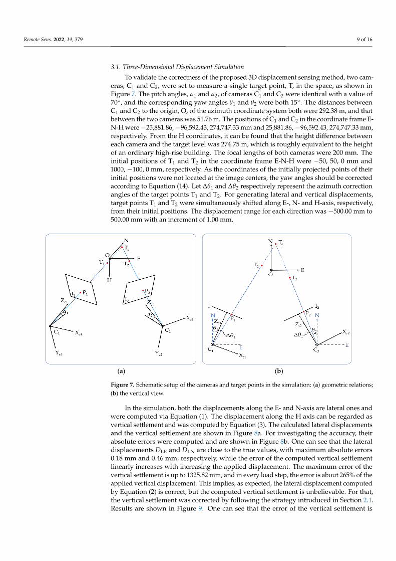
3.1. Three-Dimensional Displacement Simulation

To validate the correctness of the proposed 3D displacement sensing method, two cam-eras, C1 and C2, were set to measure a single target point, T, in the space, as shown inFigure 7. The pitch angles, α1 and α2, of cameras C1 and C2 were identical with a value of70◦, and the corresponding yaw angles θ1 and θ2 were both 15◦. The distances betweenC1 and C2 to the origin, O, of the azimuth coordinate system both were 292.38 m, and thatbetween the two cameras was 51.76 m. The positions of C1 and C2 in the coordinate frame E-N-H were−25,881.86,−96,592.43, 274,747.33 mm and 25,881.86,−96,592.43, 274,747.33 mm,respectively. From the H coordinates, it can be found that the height difference betweeneach camera and the target level was 274.75 m, which is roughly equivalent to the heightof an ordinary high-rise building. The focal lengths of both cameras were 200 mm. Theinitial positions of T1 and T2 in the coordinate frame E-N-H were −50, 50, 0 mm and1000, −100, 0 mm, respectively. As the coordinates of the initially projected points of theirinitial positions were not located at the image centers, the yaw angles should be correctedaccording to Equation (14). Let ∆θ1 and ∆θ2 respectively represent the azimuth correctionangles of the target points T1 and T2. For generating lateral and vertical displacements,target points T1 and T2 were simultaneously shifted along E-, N- and H-axis, respectively,from their initial positions. The displacement range for each direction was −500.00 mm to500.00 mm with an increment of 1.00 mm.

Remote Sens. 2022, 14, x FOR PEER REVIEW 9 of 16

3. Experiments and Results Here the correctness and performance of the proposed method are verified with a

simulation and an experiment in the following sections. In the simulation, the resolution of the used camera is 5120 × 5120 pixels and the pixel size is 3.45 μm; in the experiment, the resolution of both cameras is 2448 × 2050 pixels and the pixel size is also 3.45 μm. Details are given below.

3.1. Three-Dimensional Displacement Simulation To validate the correctness of the proposed 3D displacement sensing method, two

cameras, C1 and C2, were set to measure a single target point, T, in the space, as shown in Figure 7. The pitch angles, α1 and α2, of cameras C1 and C2 were identical with a value of 70°, and the corresponding yaw angles θ1 and θ2 were both 15°. The distances between C1 and C2 to the origin, O, of the azimuth coordinate system both were 292.38 m, and that between the two cameras was 51.76 m. The positions of C1 and C2 in the coordinate frame E-N-H were −25,881.86, −96,592.43, 274,747.33 mm and 25,881.86, −96,592.43, 274,747.33 mm, respectively. From the H coordinates, it can be found that the height difference be-tween each camera and the target level was 274.75 m, which is roughly equivalent to the height of an ordinary high-rise building. The focal lengths of both cameras were 200 mm. The initial positions of T1 and T2 in the coordinate frame E-N-H were −50, 50, 0 mm and 1000, −100, 0 mm, respectively. As the coordinates of the initially projected points of their initial positions were not located at the image centers, the yaw angles should be corrected according to Equation (14). Let Δθ1 and Δθ2 respectively represent the azimuth correction angles of the target points T1 and T2. For generating lateral and vertical displacements, target points T1 and T2 were simultaneously shifted along E-, N- and H-axis, respectively, from their initial positions. The displacement range for each direction was −500.00 mm to 500.00 mm with an increment of 1.00 mm.

(a) (b)

Figure 7. Schematic setup of the cameras and target points in the simulation: (a) geometric relations; (b) the vertical view.

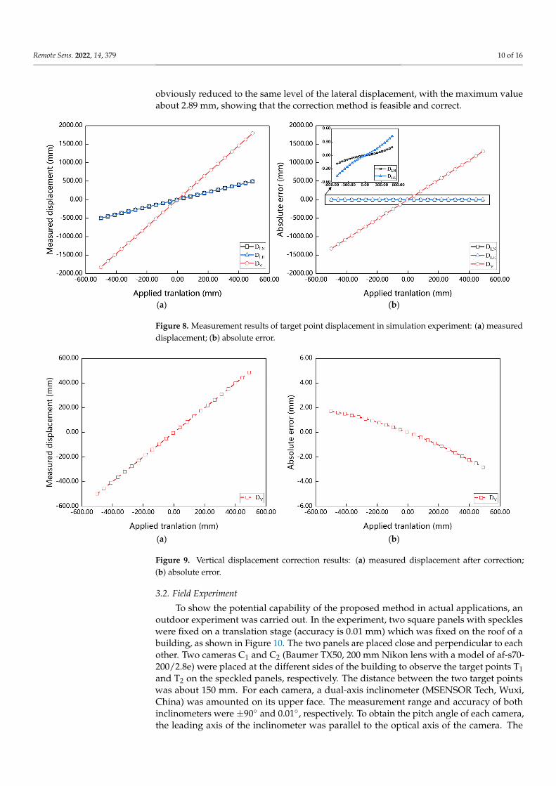
In the simulation, both the displacements along the E- and N-axis are lateral ones and were computed via Equation (1). The displacement along the H axis can be regarded as vertical settlement and was computed by Equation (3). The calculated lateral displace-ments and the vertical settlement are shown in Figure 8a. For investigating the accuracy, their absolute errors were computed and are shown in Figure 8b. One can see that the lateral displacements DLE and DLN are close to the true values, with maximum absolute

Figure 7. Schematic setup of the cameras and target points in the simulation: (a) geometric relations;(b) the vertical view.

In the simulation, both the displacements along the E- and N-axis are lateral ones andwere computed via Equation (1). The displacement along the H axis can be regarded asvertical settlement and was computed by Equation (3). The calculated lateral displacementsand the vertical settlement are shown in Figure 8a. For investigating the accuracy, theirabsolute errors were computed and are shown in Figure 8b. One can see that the lateraldisplacements DLE and DLN are close to the true values, with maximum absolute errors0.18 mm and 0.46 mm, respectively, while the error of the computed vertical settlementlinearly increases with increasing the applied displacement. The maximum error of thevertical settlement is up to 1325.82 mm, and in every load step, the error is about 265% of theapplied vertical displacement. This implies, as expected, the lateral displacement computedby Equation (2) is correct, but the computed vertical settlement is unbelievable. For that,the vertical settlement was corrected by following the strategy introduced in Section 2.1.Results are shown in Figure 9. One can see that the error of the vertical settlement is

Remote Sens. 2022, 14, 379 10 of 16

obviously reduced to the same level of the lateral displacement, with the maximum valueabout 2.89 mm, showing that the correction method is feasible and correct.

Remote Sens. 2022, 14, x FOR PEER REVIEW 10 of 16

errors 0.18 mm and 0.46 mm, respectively, while the error of the computed vertical settle-ment linearly increases with increasing the applied displacement. The maximum error of the vertical settlement is up to 1325.82 mm, and in every load step, the error is about 265% of the applied vertical displacement. This implies, as expected, the lateral displacement computed by Equation (2) is correct, but the computed vertical settlement is unbelievable. For that, the vertical settlement was corrected by following the strategy introduced in Sec-tion 2.1. Results are shown in Figure 9. One can see that the error of the vertical settlement is obviously reduced to the same level of the lateral displacement, with the maximum value about 2.89 mm, showing that the correction method is feasible and correct.

(a) (b)

Figure 8. Measurement results of target point displacement in simulation experiment: (a) measured displacement; (b) absolute error.

(a) (b)

Figure 9. Vertical displacement correction results: (a) measured displacement after correction; (b) absolute error.

3.2. Field Experiment To show the potential capability of the proposed method in actual applications, an

outdoor experiment was carried out. In the experiment, two square panels with speckles were fixed on a translation stage (accuracy is 0.01 mm) which was fixed on the roof of a

Figure 8. Measurement results of target point displacement in simulation experiment: (a) measureddisplacement; (b) absolute error.

Remote Sens. 2022, 14, x FOR PEER REVIEW 10 of 16

errors 0.18 mm and 0.46 mm, respectively, while the error of the computed vertical settle-ment linearly increases with increasing the applied displacement. The maximum error of the vertical settlement is up to 1325.82 mm, and in every load step, the error is about 265% of the applied vertical displacement. This implies, as expected, the lateral displacement computed by Equation (2) is correct, but the computed vertical settlement is unbelievable. For that, the vertical settlement was corrected by following the strategy introduced in Sec-tion 2.1. Results are shown in Figure 9. One can see that the error of the vertical settlement is obviously reduced to the same level of the lateral displacement, with the maximum value about 2.89 mm, showing that the correction method is feasible and correct.

(a) (b)

Figure 8. Measurement results of target point displacement in simulation experiment: (a) measured displacement; (b) absolute error.

(a) (b)

Figure 9. Vertical displacement correction results: (a) measured displacement after correction; (b) absolute error.

3.2. Field Experiment To show the potential capability of the proposed method in actual applications, an

outdoor experiment was carried out. In the experiment, two square panels with speckles were fixed on a translation stage (accuracy is 0.01 mm) which was fixed on the roof of a

Figure 9. Vertical displacement correction results: (a) measured displacement after correction;(b) absolute error.

3.2. Field Experiment

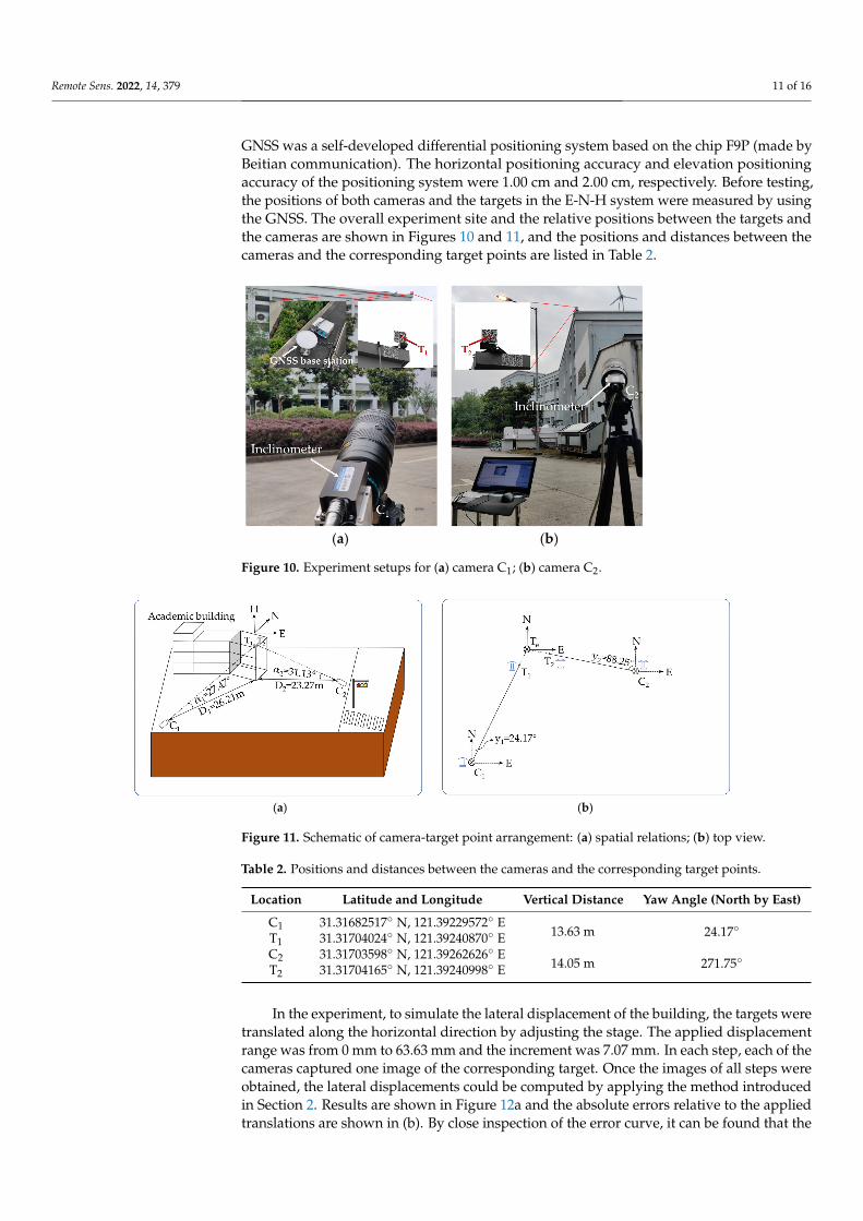
To show the potential capability of the proposed method in actual applications, anoutdoor experiment was carried out. In the experiment, two square panels with speckleswere fixed on a translation stage (accuracy is 0.01 mm) which was fixed on the roof of abuilding, as shown in Figure 10. The two panels are placed close and perpendicular to eachother. Two cameras C1 and C2 (Baumer TX50, 200 mm Nikon lens with a model of af-s70-200/2.8e) were placed at the different sides of the building to observe the target points T1and T2 on the speckled panels, respectively. The distance between the two target pointswas about 150 mm. For each camera, a dual-axis inclinometer (MSENSOR Tech, Wuxi,China) was amounted on its upper face. The measurement range and accuracy of bothinclinometers were ±90◦ and 0.01◦, respectively. To obtain the pitch angle of each camera,the leading axis of the inclinometer was parallel to the optical axis of the camera. The

Remote Sens. 2022, 14, 379 11 of 16

GNSS was a self-developed differential positioning system based on the chip F9P (made byBeitian communication). The horizontal positioning accuracy and elevation positioningaccuracy of the positioning system were 1.00 cm and 2.00 cm, respectively. Before testing,the positions of both cameras and the targets in the E-N-H system were measured by usingthe GNSS. The overall experiment site and the relative positions between the targets andthe cameras are shown in Figures 10 and 11, and the positions and distances between thecameras and the corresponding target points are listed in Table 2.

Remote Sens. 2022, 14, x FOR PEER REVIEW 11 of 16

building, as shown in Figure 10. The two panels are placed close and perpendicular to each other. Two cameras C1 and C2 (Baumer TX50, 200 mm Nikon lens with a model of af-s70-200/2.8e) were placed at the different sides of the building to observe the target points T1 and T2 on the speckled panels, respectively. The distance between the two target points was about 150 mm. For each camera, a dual-axis inclinometer (MSENSOR Tech, Wuxi, China) was amounted on its upper face. The measurement range and accuracy of both inclinometers were ±90° and 0.01°, respectively. To obtain the pitch angle of each camera, the leading axis of the inclinometer was parallel to the optical axis of the camera. The GNSS was a self-developed differential positioning system based on the chip F9P (made by Beitian communication). The horizontal positioning accuracy and elevation position-ing accuracy of the positioning system were 1.00 cm and 2.00 cm, respectively. Before test-ing, the positions of both cameras and the targets in the E-N-H system were measured by using the GNSS. The overall experiment site and the relative positions between the targets and the cameras are shown in Figures 10 and 11, and the positions and distances between the cameras and the corresponding target points are listed in Table 2

(a) (b)

Figure 10. Experiment setups for (a) camera C1; (b) camera C2.

(a) (b)

Figure 11. Schematic of camera-target point arrangement: (a) spatial relations; (b) top view.

Figure 10. Experiment setups for (a) camera C1; (b) camera C2.

Remote Sens. 2022, 14, x FOR PEER REVIEW 11 of 16

building, as shown in Figure 10. The two panels are placed close and perpendicular to each other. Two cameras C1 and C2 (Baumer TX50, 200 mm Nikon lens with a model of af-s70-200/2.8e) were placed at the different sides of the building to observe the target points T1 and T2 on the speckled panels, respectively. The distance between the two target points was about 150 mm. For each camera, a dual-axis inclinometer (MSENSOR Tech, Wuxi, China) was amounted on its upper face. The measurement range and accuracy of both inclinometers were ±90° and 0.01°, respectively. To obtain the pitch angle of each camera, the leading axis of the inclinometer was parallel to the optical axis of the camera. The GNSS was a self-developed differential positioning system based on the chip F9P (made by Beitian communication). The horizontal positioning accuracy and elevation position-ing accuracy of the positioning system were 1.00 cm and 2.00 cm, respectively. Before test-ing, the positions of both cameras and the targets in the E-N-H system were measured by using the GNSS. The overall experiment site and the relative positions between the targets and the cameras are shown in Figures 10 and 11, and the positions and distances between the cameras and the corresponding target points are listed in Table 2

(a) (b)

Figure 10. Experiment setups for (a) camera C1; (b) camera C2.

(a) (b)

Figure 11. Schematic of camera-target point arrangement: (a) spatial relations; (b) top view.

Figure 11. Schematic of camera-target point arrangement: (a) spatial relations; (b) top view.

Table 2. Positions and distances between the cameras and the corresponding target points.

Location Latitude and Longitude Vertical Distance Yaw Angle (North by East)

C1 31.31682517◦ N, 121.39229572◦ E13.63 m 24.17◦T1 31.31704024◦ N, 121.39240870◦ E

C2 31.31703598◦ N, 121.39262626◦ E14.05 m 271.75◦T2 31.31704165◦ N, 121.39240998◦ E

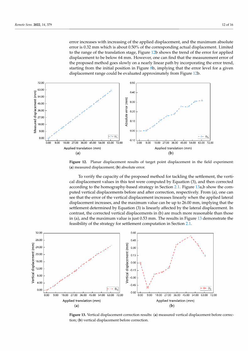
In the experiment, to simulate the lateral displacement of the building, the targets weretranslated along the horizontal direction by adjusting the stage. The applied displacementrange was from 0 mm to 63.63 mm and the increment was 7.07 mm. In each step, each of thecameras captured one image of the corresponding target. Once the images of all steps wereobtained, the lateral displacements could be computed by applying the method introducedin Section 2. Results are shown in Figure 12a and the absolute errors relative to the appliedtranslations are shown in (b). By close inspection of the error curve, it can be found that the

Remote Sens. 2022, 14, 379 12 of 16

error increases with increasing of the applied displacement, and the maximum absoluteerror is 0.32 mm which is about 0.50% of the corresponding actual displacement. Limitedto the range of the translation stage, Figure 12b shows the trend of the error for applieddisplacement to be below 64 mm. However, one can find that the measurement error ofthe proposed method goes slowly on a nearly linear path by incorporating the error trend,starting from the initial position in Figure 8b, implying that the error level for a givendisplacement range could be evaluated approximately from Figure 12b.

Remote Sens. 2022, 14, x FOR PEER REVIEW 12 of 16

Table 2. Positions and distances between the cameras and the corresponding target points.

Location Latitude and Longitude Vertical Distance Yaw Angle (North by East) C1 31.31682517°N, 121.39229572°E

13.63 m 24.17° T1 31.31704024°N, 121.39240870°E C2 31.31703598°N, 121.39262626°E

14.05 m 271.75° T2 31.31704165°N, 121.39240998°E

In the experiment, to simulate the lateral displacement of the building, the targets were translated along the horizontal direction by adjusting the stage. The applied dis-placement range was from 0 mm to 63.63 mm and the increment was 7.07 mm. In each step, each of the cameras captured one image of the corresponding target. Once the images of all steps were obtained, the lateral displacements could be computed by applying the method introduced in Section 2. Results are shown in Figure 12a and the absolute errors relative to the applied translations are shown in (b). By close inspection of the error curve, it can be found that the error increases with increasing of the applied displacement, and the maximum absolute error is 0.32 mm which is about 0.50% of the corresponding actual displacement. Limited to the range of the translation stage, Figure 12b shows the trend of the error for applied displacement to be below 64 mm. However, one can find that the measurement error of the proposed method goes slowly on a nearly linear path by incor-porating the error trend, starting from the initial position in Figure 8b, implying that the error level for a given displacement range could be evaluated approximately from Figure 12b.

(a) (b)

Figure 12. Planar displacement results of target point displacement in the field experiment: (a) meas-ured displacement; (b) absolute error.

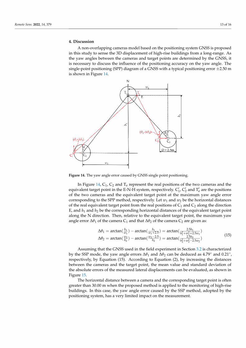
To verify the capacity of the proposed method for tackling the settlement, the vertical displacement values in this test were computed by Equation (3), and then corrected ac-cording to the homography-based strategy in Section 2.1. Figure 13a,b show the computed vertical displacements before and after correction, respectively. From (a), one can see that the error of the vertical displacement increases linearly when the applied lateral displace-ment increases, and the maximum value can be up to 26.00 mm, implying that the settle-ment determined by Equation (3) is linearly affected by the lateral displacement. In con-trast, the corrected vertical displacements in (b) are much more reasonable than those in (a), and the maximum value is just 0.53 mm. The results in Figure 13 demonstrate the feasibility of the strategy for settlement computation in Section 2.1.

Figure 12. Planar displacement results of target point displacement in the field experiment:(a) measured displacement; (b) absolute error.

To verify the capacity of the proposed method for tackling the settlement, the verti-cal displacement values in this test were computed by Equation (3), and then correctedaccording to the homography-based strategy in Section 2.1. Figure 13a,b show the com-puted vertical displacements before and after correction, respectively. From (a), one cansee that the error of the vertical displacement increases linearly when the applied lateraldisplacement increases, and the maximum value can be up to 26.00 mm, implying that thesettlement determined by Equation (3) is linearly affected by the lateral displacement. Incontrast, the corrected vertical displacements in (b) are much more reasonable than thosein (a), and the maximum value is just 0.53 mm. The results in Figure 13 demonstrate thefeasibility of the strategy for settlement computation in Section 2.1.

Remote Sens. 2022, 14, x FOR PEER REVIEW 13 of 16

(a) (b)

Figure 13. Vertical displacement correction results: (a) measured vertical displacement before cor-rection; (b) vertical displacement before correction.

4. Discussion A non-overlapping cameras model based on the positioning system GNSS is pro-

posed in this study to sense the 3D displacement of high-rise buildings from a long-range. As the yaw angles between the cameras and target points are determined by the GNSS, it is necessary to discuss the influence of the positioning accuracy on the yaw angle. The single-point positioning (SPP) diagram of a GNSS with a typical positioning error ±2.50 m is shown in Figure 14.

Figure 14. The yaw angle error caused by GNSS single point positioning.

In Figure 14, C1, C2 and Te represent the real positions of the two cameras and the equivalent target point in the E-N-H system, respectively. C1

’ , C2’ and Te

’ are the positions of the two cameras and the equivalent target point at the maximum yaw angle error cor-responding to the SPP method, respectively. Let w1 and w2 be the horizontal distances of the real equivalent target point from the real positions of C1 and C2 along the direction E, and h1 and h2 be the corresponding horizontal distances of the equivalent target point along the N direction. Then, relative to the equivalent target point, the maximum yaw angle error Δθ1 of the camera C1 and that Δθ2 of the camera C2 are given as:

Figure 13. Vertical displacement correction results: (a) measured vertical displacement before correc-tion; (b) vertical displacement before correction.

Remote Sens. 2022, 14, 379 13 of 16

4. Discussion

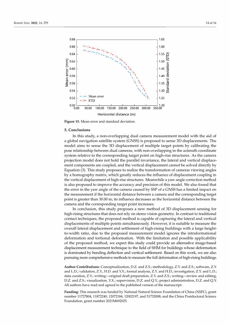
A non-overlapping cameras model based on the positioning system GNSS is proposedin this study to sense the 3D displacement of high-rise buildings from a long-range. Asthe yaw angles between the cameras and target points are determined by the GNSS, itis necessary to discuss the influence of the positioning accuracy on the yaw angle. Thesingle-point positioning (SPP) diagram of a GNSS with a typical positioning error ±2.50 mis shown in Figure 14.

Remote Sens. 2022, 14, x FOR PEER REVIEW 13 of 16

(a) (b)

Figure 13. Vertical displacement correction results: (a) measured vertical displacement before cor-rection; (b) vertical displacement before correction.

4. Discussion A non-overlapping cameras model based on the positioning system GNSS is pro-

posed in this study to sense the 3D displacement of high-rise buildings from a long-range. As the yaw angles between the cameras and target points are determined by the GNSS, it is necessary to discuss the influence of the positioning accuracy on the yaw angle. The single-point positioning (SPP) diagram of a GNSS with a typical positioning error ±2.50 m is shown in Figure 14.

Figure 14. The yaw angle error caused by GNSS single point positioning.

In Figure 14, C1, C2 and Te represent the real positions of the two cameras and the equivalent target point in the E-N-H system, respectively. C1

’ , C2’ and Te

’ are the positions of the two cameras and the equivalent target point at the maximum yaw angle error cor-responding to the SPP method, respectively. Let w1 and w2 be the horizontal distances of the real equivalent target point from the real positions of C1 and C2 along the direction E, and h1 and h2 be the corresponding horizontal distances of the equivalent target point along the N direction. Then, relative to the equivalent target point, the maximum yaw angle error Δθ1 of the camera C1 and that Δθ2 of the camera C2 are given as:

Figure 14. The yaw angle error caused by GNSS single point positioning.

In Figure 14, C1, C2 and Te represent the real positions of the two cameras and theequivalent target point in the E-N-H system, respectively. C′1, C′2 and T′e are the positionsof the two cameras and the equivalent target point at the maximum yaw angle errorcorresponding to the SPP method, respectively. Let w1 and w2 be the horizontal distancesof the real equivalent target point from the real positions of C1 and C2 along the directionE, and h1 and h2 be the corresponding horizontal distances of the equivalent target pointalong the N direction. Then, relative to the equivalent target point, the maximum yawangle error ∆θ1 of the camera C1 and that ∆θ2 of the camera C2 are given as:

∆θ1 = arctan( h1w1)− arctan( h1

w1+2.5 ) = arctan( 2.5h1h2

1+w21+2.5w1

)

∆θ2 = arctan(w2h2)− arctan(w2−2.5

h2) = arctan( 2.5h2

h22+w2

2−2.5w2)

(15)

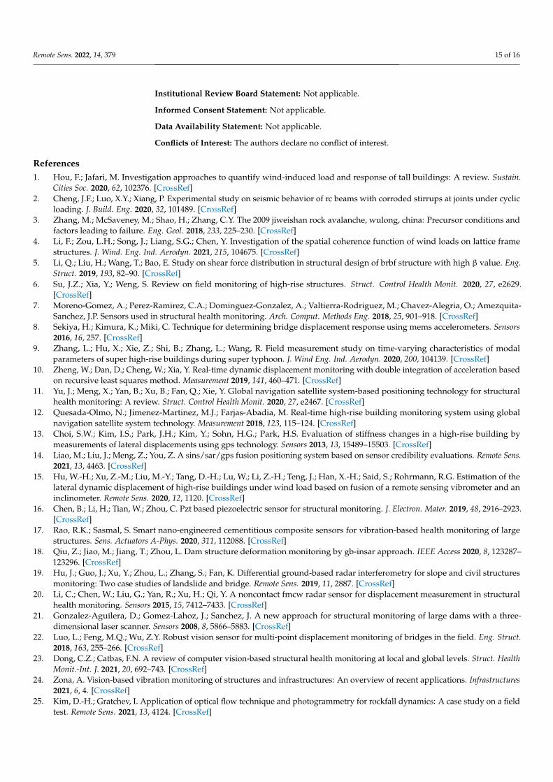
Assuming that the GNSS used in the field experiment in Section 3.2 is characterizedby the SSP mode, the yaw angle errors ∆θ1 and ∆θ2 can be deduced as 4.79◦ and 0.21◦,respectively, by Equation (15). According to Equation (2), by increasing the distancesbetween the cameras and the target point, the mean value and standard deviation ofthe absolute errors of the measured lateral displacements can be evaluated, as shown inFigure 15.

The horizontal distance between a camera and the corresponding target point is oftengreater than 30.00 m when the proposed method is applied to the monitoring of high-risebuildings. In this case, the yaw angle error caused by the SSP method, adopted by thepositioning system, has a very limited impact on the measurement.

Remote Sens. 2022, 14, 379 14 of 16

Remote Sens. 2022, 14, x FOR PEER REVIEW 14 of 16

1 1 11 2 2

1 1 1 1 1

2 2 22 2 2

2 2 2 2 2

2.5arctan( ) arctan( ) arctan( )

2.5 2.52.5 2.5

arctan( ) arctan( ) arctan( )2.5

h h hw w h w ww w hh h h w w

Δ = − =+ + +−

Δ = − =+ −

θ

θ (15)

Assuming that the GNSS used in the field experiment in Section 3.2 is characterized by the SSP mode, the yaw angle errors Δθ1 and Δθ2 can be deduced as 4.79° and 0.21°, respectively, by Equation (15). According to Equation (2), by increasing the distances be-tween the cameras and the target point, the mean value and standard deviation of the absolute errors of the measured lateral displacements can be evaluated, as shown in Fig-ure 15.

Figure 15. Mean error and standard deviation.

The horizontal distance between a camera and the corresponding target point is often greater than 30.00 m when the proposed method is applied to the monitoring of high-rise buildings. In this case, the yaw angle error caused by the SSP method, adopted by the positioning system, has a very limited impact on the measurement.

5. Conclusions In this study, a non-overlapping dual camera measurement model with the aid of a

global navigation satellite system (GNSS) is proposed to sense 3D displacements. The model aims to sense the 3D displacement of multiple target points by calibrating the pose relationship between dual cameras, with non-overlapping in the azimuth coordinate sys-tem relative to the corresponding target point on high-rise structures. As the camera pro-jection model does not hold the parallel invariance, the lateral and vertical displacement components are coupled, and the vertical displacement cannot be solved directly by Equa-tion (3). This study proposes to realize the transformation of cameras viewing angles by a homography matrix, which greatly reduces the influence of displacement coupling in the vertical displacement of high-rise structures. Meanwhile a yaw angle correction method is also proposed to improve the accuracy and precision of this model. We also found that the error in the yaw angle of the camera caused by SSP of a GNSS has a limited impact on the measurement if the horizontal distance between a camera and the corresponding tar-get point is greater than 30.00 m; its influence decreases as the horizontal distance between the camera and the corresponding target point increases.

Figure 15. Mean error and standard deviation.

5. Conclusions

In this study, a non-overlapping dual camera measurement model with the aid ofa global navigation satellite system (GNSS) is proposed to sense 3D displacements. Themodel aims to sense the 3D displacement of multiple target points by calibrating thepose relationship between dual cameras, with non-overlapping in the azimuth coordinatesystem relative to the corresponding target point on high-rise structures. As the cameraprojection model does not hold the parallel invariance, the lateral and vertical displace-ment components are coupled, and the vertical displacement cannot be solved directly byEquation (3). This study proposes to realize the transformation of cameras viewing anglesby a homography matrix, which greatly reduces the influence of displacement coupling inthe vertical displacement of high-rise structures. Meanwhile a yaw angle correction methodis also proposed to improve the accuracy and precision of this model. We also found thatthe error in the yaw angle of the camera caused by SSP of a GNSS has a limited impact onthe measurement if the horizontal distance between a camera and the corresponding targetpoint is greater than 30.00 m; its influence decreases as the horizontal distance between thecamera and the corresponding target point increases.

In conclusion, this study proposes a new method of 3D displacement sensing forhigh-rising structures that does not rely on stereo vision geometry. In contrast to traditionalcontact techniques, the proposed method is capable of capturing the lateral and verticaldisplacements of multiple points simultaneously. However, it is suitable to measure theoverall lateral displacement and settlement of high-rising buildings with a large height-to-width ratio, due to the proposed measurement model ignores the intraformationaldeformation and tortional deformation. With the limitation and possible applicabilityof the proposed method, we expect this study could provide an alternative image-baseddisplacement measurement technique to the field of SHM for buildings whose deformationis dominated by bending deflection and vertical settlement. Based on this work, we are alsopursuing more comprehensive methods to measure the full deformation of high-rising buildings.

Author Contributions: Conceptualization, D.Z. and Z.S.; methodology, Z.Y. and Z.S.; software, Z.Y.and L.D.; validation, Z.Y., H.D. and Y.X.; formal analysis, Z.Y. and H.D.; investigation, Z.Y. and L.D.;data curation, Z.Y.; writing—original draft preparation, Z.Y. and Z.S.; writing—review and editing,D.Z. and Z.S.; visualization, Y.X.; supervision, D.Z. and Q.Y.; project administration, D.Z. and Q.Y.All authors have read and agreed to the published version of the manuscript.

Funding: This research was funded by National Natural Science Foundation of China (NSFC), grantnumber 11727804, 11872240, 12072184, 12002197, and 51732008; and the China Postdoctoral ScienceFoundation, grant number 2021M692025.

Remote Sens. 2022, 14, 379 15 of 16

Institutional Review Board Statement: Not applicable.

Informed Consent Statement: Not applicable.

Data Availability Statement: Not applicable.

Conflicts of Interest: The authors declare no conflict of interest.

References1. Hou, F.; Jafari, M. Investigation approaches to quantify wind-induced load and response of tall buildings: A review. Sustain.

Cities Soc. 2020, 62, 102376. [CrossRef]2. Cheng, J.F.; Luo, X.Y.; Xiang, P. Experimental study on seismic behavior of rc beams with corroded stirrups at joints under cyclic

loading. J. Build. Eng. 2020, 32, 101489. [CrossRef]3. Zhang, M.; McSaveney, M.; Shao, H.; Zhang, C.Y. The 2009 jiweishan rock avalanche, wulong, china: Precursor conditions and

factors leading to failure. Eng. Geol. 2018, 233, 225–230. [CrossRef]4. Li, F.; Zou, L.H.; Song, J.; Liang, S.G.; Chen, Y. Investigation of the spatial coherence function of wind loads on lattice frame

structures. J. Wind. Eng. Ind. Aerodyn. 2021, 215, 104675. [CrossRef]5. Li, Q.; Liu, H.; Wang, T.; Bao, E. Study on shear force distribution in structural design of brbf structure with high β value. Eng.

Struct. 2019, 193, 82–90. [CrossRef]6. Su, J.Z.; Xia, Y.; Weng, S. Review on field monitoring of high-rise structures. Struct. Control Health Monit. 2020, 27, e2629.

[CrossRef]7. Moreno-Gomez, A.; Perez-Ramirez, C.A.; Dominguez-Gonzalez, A.; Valtierra-Rodriguez, M.; Chavez-Alegria, O.; Amezquita-

Sanchez, J.P. Sensors used in structural health monitoring. Arch. Comput. Methods Eng. 2018, 25, 901–918. [CrossRef]8. Sekiya, H.; Kimura, K.; Miki, C. Technique for determining bridge displacement response using mems accelerometers. Sensors

2016, 16, 257. [CrossRef]9. Zhang, L.; Hu, X.; Xie, Z.; Shi, B.; Zhang, L.; Wang, R. Field measurement study on time-varying characteristics of modal

parameters of super high-rise buildings during super typhoon. J. Wind Eng. Ind. Aerodyn. 2020, 200, 104139. [CrossRef]10. Zheng, W.; Dan, D.; Cheng, W.; Xia, Y. Real-time dynamic displacement monitoring with double integration of acceleration based

on recursive least squares method. Measurement 2019, 141, 460–471. [CrossRef]11. Yu, J.; Meng, X.; Yan, B.; Xu, B.; Fan, Q.; Xie, Y. Global navigation satellite system-based positioning technology for structural

health monitoring: A review. Struct. Control Health Monit. 2020, 27, e2467. [CrossRef]12. Quesada-Olmo, N.; Jimenez-Martinez, M.J.; Farjas-Abadia, M. Real-time high-rise building monitoring system using global

navigation satellite system technology. Measurement 2018, 123, 115–124. [CrossRef]13. Choi, S.W.; Kim, I.S.; Park, J.H.; Kim, Y.; Sohn, H.G.; Park, H.S. Evaluation of stiffness changes in a high-rise building by

measurements of lateral displacements using gps technology. Sensors 2013, 13, 15489–15503. [CrossRef]14. Liao, M.; Liu, J.; Meng, Z.; You, Z. A sins/sar/gps fusion positioning system based on sensor credibility evaluations. Remote Sens.

2021, 13, 4463. [CrossRef]15. Hu, W.-H.; Xu, Z.-M.; Liu, M.-Y.; Tang, D.-H.; Lu, W.; Li, Z.-H.; Teng, J.; Han, X.-H.; Said, S.; Rohrmann, R.G. Estimation of the

lateral dynamic displacement of high-rise buildings under wind load based on fusion of a remote sensing vibrometer and aninclinometer. Remote Sens. 2020, 12, 1120. [CrossRef]

16. Chen, B.; Li, H.; Tian, W.; Zhou, C. Pzt based piezoelectric sensor for structural monitoring. J. Electron. Mater. 2019, 48, 2916–2923.[CrossRef]

17. Rao, R.K.; Sasmal, S. Smart nano-engineered cementitious composite sensors for vibration-based health monitoring of largestructures. Sens. Actuators A-Phys. 2020, 311, 112088. [CrossRef]

18. Qiu, Z.; Jiao, M.; Jiang, T.; Zhou, L. Dam structure deformation monitoring by gb-insar approach. IEEE Access 2020, 8, 123287–123296. [CrossRef]

19. Hu, J.; Guo, J.; Xu, Y.; Zhou, L.; Zhang, S.; Fan, K. Differential ground-based radar interferometry for slope and civil structuresmonitoring: Two case studies of landslide and bridge. Remote Sens. 2019, 11, 2887. [CrossRef]

20. Li, C.; Chen, W.; Liu, G.; Yan, R.; Xu, H.; Qi, Y. A noncontact fmcw radar sensor for displacement measurement in structuralhealth monitoring. Sensors 2015, 15, 7412–7433. [CrossRef]

21. Gonzalez-Aguilera, D.; Gomez-Lahoz, J.; Sanchez, J. A new approach for structural monitoring of large dams with a three-dimensional laser scanner. Sensors 2008, 8, 5866–5883. [CrossRef]

22. Luo, L.; Feng, M.Q.; Wu, Z.Y. Robust vision sensor for multi-point displacement monitoring of bridges in the field. Eng. Struct.2018, 163, 255–266. [CrossRef]

23. Dong, C.Z.; Catbas, F.N. A review of computer vision-based structural health monitoring at local and global levels. Struct. HealthMonit.-Int. J. 2021, 20, 692–743. [CrossRef]

24. Zona, A. Vision-based vibration monitoring of structures and infrastructures: An overview of recent applications. Infrastructures2021, 6, 4. [CrossRef]

25. Kim, D.-H.; Gratchev, I. Application of optical flow technique and photogrammetry for rockfall dynamics: A case study on a fieldtest. Remote Sens. 2021, 13, 4124. [CrossRef]

Remote Sens. 2022, 14, 379 16 of 16

26. Sanchez-Aparicio, L.J.; Herrero-Huerta, M.; Esposito, R.; Schipper, H.R.; Gonzalez-Aguilera, D. Photogrammetric solution foranalysis of out-of-plane movements of a masonry structure in a large-scale laboratory experiment. Remote Sens. 2019, 11, 1871.[CrossRef]

27. Shan, B.; Wang, L.; Huo, X.; Yuan, W.; Xue, Z. A bridge deflection monitoring system based on ccd. Adv. Mater. Sci. Eng. 2016,2016, 4857373. [CrossRef]

28. Jo, B.-W.; Lee, Y.-S.; Jo, J.H.; Khan, R.M.A. Computer vision-based bridge displacement measurements using rotation-invariantimage processing technique. Sustainability 2018, 10, 1785. [CrossRef]

29. Su, Z.; Pan, J.; Lu, L.; Dai, M.; He, X.; Zhang, D. Refractive three-dimensional reconstruction for underwater stereo digital imagecorrelation. Opt. Express 2021, 29, 12131–12144. [CrossRef]

30. Wang, S.; Zhang, S.Q.; Li, X.D.; Zou, Y.; Zhang, D.S. Development of monocular video deflectometer based on inclination sensors.Smart Struct. Syst. 2019, 24, 607–616.

31. Fioriti, V.; Roselli, I.; Tati, A.; Romano, R.; De Canio, G. Motion magnification analysis for structural monitoring of ancientconstructions. Measurement 2018, 129, 375–380. [CrossRef]

32. Park, J.-W.; Lee, J.-J.; Jung, H.-J.; Myung, H. Vision-based displacement measurement method for high-rise building structuresusing partitioning approach. Ndt E Int. 2010, 43, 642–647. [CrossRef]

33. Guo, J.; Xiang, Y.; Fujita, K.; Takewaki, I. Vision-based building seismic displacement measurement by stratification of projectiverectification using lines. Sensors 2020, 20, 5775. [CrossRef]

34. Ye, X.-W.; Jin, T.; Ang, P.-P.; Bian, X.-C.; Chen, Y.-M. Computer vision-based monitoring of the 3-d structural deformation of anancient structure induced by shield tunneling construction. Struct. Control Health Monit. 2021, 28, e2702. [CrossRef]

35. Chen, X.; Achilli, V.; Fabris, M.; Menin, A.; Monego, M.; Tessari, G.; Floris, M. Combining sentinel-1 interferometry andground-based geomatics techniques for monitoring buildings affected by mass movements. Remote Sens. 2021, 13, 452. [CrossRef]

36. Schreier, H.; Orteu, J.-J.; Sutton, M.A. Image Correlation for Shape, Motion and Deformation Measurements. Basic Concepts, Theory andApplications; Springer: Berlin/Heidelberg, Germany, 2009.

37. Su, Z.L.; Lu, L.; He, X.Y.; Yang, F.J.; Zhang, D.S. Recursive-iterative digital image correlation based on salient features. Opt. Eng.2020, 59, 034111. [CrossRef]

38. Hartley, R.; Zisserman, A. Multiple View Geometry in Computer Vision; Cambridge University Press: Cambridge, UK, 2003.39. Zhang, X.L.; Zhu, P.A.; Hu, C.S. A Simple algorithm for distance and Azimuth of missile-to-target based on longitude and latitude.

Ordnance Ind. Autom 2019, 38, 7–9. (In Chinese)