Glueballs at finite temperature in SUð3Þ Yang-Mills theory

Xiang-Fei Meng,1,2 Gang Li,3,4 Yuan-Jiang Zhang,3,4 Ying Chen,3,4 Chuan Liu,5 Yu-Bin Liu,1

Jian-Ping Ma,6 and Jian-Bo Zhang7

(CLQCD Collaboration)

1School of Physics, Nankai University, Tianjin 300071, People’s Republic of China2National Supercomputing Center, Tianjin 300457, People’s Republic of China

3Institute of High Energy Physics, Chinese Academy of Sciences, Beijing 100049, People’s Republic of China4Theoretical Center for Science Facilities, Chinese Academy of Sciences, Beijing 100049, People’s Republic of China

5School of Physics, Peking University, Beijing 100871, People’s Republic of China6Institute of Theoretical Physics, Chinese Academy of Sciences, Beijing 100080, People’s Republic of China

7Department of Physics, Zhejiang University, Hangzhou, Zhejiang 310027, People’s Republic of China(Received 16 March 2009; revised manuscript received 24 November 2009; published 14 December 2009)

Thermal properties of glueballs in SUð3Þ Yang-Mills theory are investigated in a large temperature

range from 0:3Tc to 1:9Tc on anisotropic lattices. The glueball operators are optimized for the projection

of the ground states by the variational method with a smearing scheme. Their thermal correlators are

calculated in all 20 symmetry channels. It is found in all channels that the pole masses MG of glueballs

remain almost constant when the temperature is approaching the critical temperature Tc from below, and

start to reduce gradually with the temperature going above Tc. The correlators in the 0þþ, 0�þ, and 2þþ

channels are also analyzed based on the Breit-Wigner Ansatz by assuming a thermal width � to the pole

mass !0 of each thermal glueball ground state. While the values of !0 are insensitive to T in the whole

temperature range, the thermal widths � exhibit distinct behaviors at temperatures below and above Tc.

The widths are very small (approximately a few percent of !0 or even smaller) when T < Tc, but grow

abruptly when T > Tc and reach values of roughly ��!0=2 at T � 1:9Tc.

DOI: 10.1103/PhysRevD.80.114502 PACS numbers: 12.38.Gc, 11.15.Ha, 14.40.Rt, 25.75.Nq

I. INTRODUCTION

The past two or three decades witnessed intensive andextensive studies on the phase transition of quantum chro-modynamics (QCD) [1], which is believed to be the fun-damental theory of strong interaction. Based on the twocharacteristics of QCD, namely, the conjectured colorconfinement at low energies and the asymptotic freedomof gluons and quarks at high energies, QCD at finitetemperature is usually described by two extreme pictures.One is with the weakly interacting meson gas in the lowtemperature regime and another is with perturbative quark-gluon plasma (QGP) in the high temperature regime. Thetwo regimes are bridged by a deconfinement phase tran-sition (or crossover). The study of the equation of stateshows that the perturbative picture of QGP can only beachieved at very high temperatures T � 2Tc. In otherwords, the dynamical degrees of freedom up to the tem-perature of a few times of Tc are not just the quasifreegluons and quarks [2]. Some other theoretical studies alsosupport this scenario and conjecture that in the intermedi-ate temperature range above Tc there may exist differenttypes of excitations corresponding to different distancescales [3,4] rendering the thermal states much more com-plicated. Apart from the quasifree quarks and gluons at thesmall distance scale, the large scale excitations can be

effective low-energy modes in the mesonic channels as aresult of the strongly interacting partons [5]. The propertiesof the interaction among quarks and gluons at low and hightemperatures can be studied with thermal correlators.There have been many works on the correlators of

charmonia at finite temperature. Phenomenological studiespredicted the binding between quarks is reduced to dis-solve J=c at temperatures close to Tc and proposed thesuppression of charmonia as a signal of QGP [6,7]. Forexample, potential model studies show that excited stateslike c 0 and �c are dissociated at Tc, while the ground statecharmonia J=� and �c survive up to T ¼ 1:1Tc [8–13].However, it is unclear whether the potential model workswell at finite temperatures [14]. In contrast, many recentnumerical studies indicate that J=� and �c might stillsurvive above 1:5Tc [15–19]. Of course, it is possiblethat the �cc states observed in lattice QCD are just scatteringstates. A further lattice study on spatial boundary-condition dependence of the energy of low-lying �cc sys-tems concludes that they are spatially localized (quasi)bound states in the temperature region of 1:11� 2:07Tc

[20]. Obviously, the results of numerical lattice QCDstudies are coincident to the picture of the QCD transitionin the intermediate temperature regime.Until now most of the lattice studies on hadronic corre-

lators are in the quenched approximation. Because of the

PHYSICAL REVIEW D 80, 114502 (2009)

1550-7998=2009=80(11)=114502(15) 114502-1 � 2009 The American Physical Society

lack of dynamical quarks in quenched QCD the binding ofquark-antiquark systems must be totally attributed to thenonperturbative properties of gluons, which are the uniquedynamical degree of freedom in the theory. Since glueballsare the bound states of gluons, a natural question is howglueballs respond to the varying temperatures. At lowtemperature T � 0, the existence of quenched glueballshas been verified by extensive lattice numerical studies,and their spectrum are also established quite well [21–28].An investigation of the evolution of glueballs versus theincreasing temperature is important to understand the QCDtransition [29,30] and the hadronization of quark-gluonplasma [31]. From the point of view of QCD sum rules,glueball masses are closely related to the gluon condensate.Lattice studies [32] and model calculations [33] indicatethat the gluon condensate keeps almost constant below Tc

and reduces gradually with the increasing temperatureabove Tc. Based on this picture, it is expected intuitivelythat glueball masses should show a similar behavior alsountil they melt into gluons [34]. In fact, there has alreadybeen a lattice study on the scalar and tensor glueballproperties at finite temperature [35]. In contrast to theexpectation and the finite T behavior of charmonium spec-trum, it is interestingly observed that the pole-mass reduc-tion starts even below TcðmGðT � TcÞ ’ 0:8mGðT � 0ÞÞ. Itis known that the spatial symmetry group on the lattice isthe 24-element cubic point group O, whose irreduciblerepresentations are R ¼ A1, A2, E, T1, and T2. Alongwith the parity P and charge conjugate transformation C,all the possible quantum numbers that glueballs can catchare RPC with PC ¼ þþ , �þ , þ� , and þþ , whichadd up to 20 symmetry channels. Motivated by the differ-ent temperature behaviors of �cc systems with differentquantum numbers, we would like to investigate the tem-perature dependence of glueballs in this paper.

Our numerical study in this work is carried out onanisotropic lattices with much finer lattice in the temporaldirection than in spatial ones. In order to explore thetemperature evolution of glueball spectrum, the tempera-ture range studied here extends from 0:3Tc to 1:9Tc, whichis realized by varying the temporal extension of the lattice.Using anisotropic lattices, the lattice parameters are care-fully determined so that there are enough time slices for areliable data analysis even at the highest temperature. Inthe present study, we are only interested in the ground statein each symmetry channel RPC. For the study optimizedglueball operators that couple mostly to the ground statesare desired. Practically, these optimized operators are builtup by the combination of smearing schemes and the varia-tional method [21–23]. In the data processing, the correla-tors of these optimized operators are analyzed through twoapproaches. First, the thermal masses MG of glueballs areextracted in all the channels and all over the temperaturerange by fitting the correlators with a single-cosh functionform, as is done in the standard hadron mass measure-

ments. Thus the T evolution of the thermal glueball spec-trums is obtained. Secondly, with respect that the finitetemperature effects may result in mass shifts and thermalwidths of glueballs, we also analyze the correlators in Aþþ

1 ,A�þ1 , Eþþ, and Tþþ

2 channels with the Breit-WignerAnsatz which assumes these glueball thermal widths, say,change MG into !0 � i� in the spectral function (seebelow). As a result, the temperature dependence of !0

and � can shed some light on the scenario of the QCDtransition.This paper is organized as follows. In Sec. II, a descrip-

tion of the determination of working parameters, such asthe critical temperature Tc, temperature range, and latticespacing as, as well as a brief introduction to the variationalmethod is given. In Sec. III, after a discussion of itsfeasibility, the results of the single-cosh fit to the thermalcorrelators are described in detail. The procedure of theBreit-Wigner fit is also given in this section. Section IVgives the conclusion and some further discussions.

II. NUMERICAL DETAILS

For heavy particles such as charmonia and glueballs, theimplementation of anisotropic lattices is found to be veryefficient in the previous numerical lattice QCD studies bothat low and finite temperatures. On the other hand, theSymanzik improvement and tadpole improvementschemes of the gauge action are verified to have bettercontinuum extrapolation behaviors for many physicalquantities. In other words, the finite lattice spacing artifactsare substantially reduced by these improvements. Withthese facts, we adopt the following improved gauge actionwhich has been extensively used in the study of glueballs[21–23],

SIA ¼ �

�5

3

�sp

�u4sþ 4

3

��tp

u2t u2s

� 1

12

�sr

�u6s� 1

12

��str

u4su2t

�; (1)

where � is related to the bare QCD coupling constant, � ¼as=at is the aspect ratio for anisotropy (we take � ¼ 5 inthis work), us and ut are the tadpole improvement parame-ters of spatial and temporal gauge links, respectively.�C ¼ P

C13 Re Trð1�WCÞ, with WC denoting the path-

ordered product of link variables along a closed contour Con the lattice. �sp includes the sum over all spatial pla-

quettes on the lattice,�tp includes the temporal plaquettes,

�sr denotes the product of link variables about planar 2�1 spatial rectangular loops, and �str refers to the shorttemporal rectangles (one temporal link, two spatial).Practically, ut is set to 1, and us is defined by the expec-

tation value of the spatial plaquette, us ¼ h13 TrPss0 i1=4.

A. Determination of critical temperature

Since the temperature T on the lattice is defined by

T ¼ 1

Ntat; (2)

MENG et al. PHYSICAL REVIEW D 80, 114502 (2009)

114502-2

where Nt is the temporal lattice size, T can be changed byvarying either Nt or the coupling constant �, which isrelated directly to the lattice spacing. In order for thecritical temperature to be determined with enough preci-sion, for a given Nt ¼ 24, we first determine the criticalcoupling �c, because � can be changed continuously. Theorder parameter is chosen as the susceptibility �P of thePolyakov line, which is defined as

�P ¼ h�2i � h�i2; (3)

where � is the Zð3Þ rotated Polyakov line,

� ¼8<:ReP exp½�2�i=3� argP 2 ½�=3; �ÞReP argP 2 ½��=3; �=3ÞReP exp½2�i=3� argP 2 ½��;��=3Þ;

(4)

and P represents the trace of the spatially averagedPolyakov line on each gauge configuration.

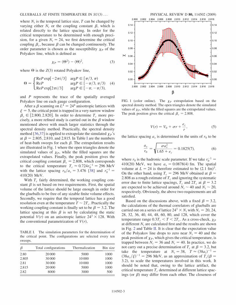
After a� scanning on L4 ¼ 244 anisotropic lattices with� ¼ 5, the critical point is trapped in a very narrow window�c 2 ½2:800; 2:820�. In order to determine Tc more pre-cisely, a more refined study is carried out in the � windowmentioned above with much larger statistics through thespectral density method. Practically, the spectral densitymethod [36,37] is applied to extrapolate the simulated �P’sat � ¼ 2:805, 2.810, and 2.815. In Table I are the numbersof heat-bath sweeps for each �. The extrapolation resultsare illustrated in Fig. 1 where the open triangles denote thesimulated values of �P, while the filled squares are theextrapolated values. Finally, the peak position gives thecritical coupling constant �c ¼ 2:808, which correspondsto the critical temperature Tc � 0:724r�1

0 ¼ 296 MeVwith the lattice spacing r0=as ¼ 3:476 [38] and r�1

0 ¼410ð20Þ MeV.

With Tc fairly determined, the working coupling con-stant � is set based on two requirements. First, the spatialvolume of the lattice should be large enough in order forthe glueballs to be free of any sizable finite volume effects.Secondly, we require that the temporal lattice has a goodresolution even at the temperature T � 2Tc. Practically theworking coupling constant is finally set to be � ¼ 3:2. Thelattice spacing at this � is set by calculating the staticpotential VðrÞ on an anisotropic lattice 243 � 128. Withthe conventional parametrization of VðrÞ,

VðrÞ ¼ V0 þ �rþ ecr; (5)

the lattice spacing as is determined in the units of r0 to be

asr0

¼ffiffiffiffiffiffiffiffiffiffiffiffiffiffiffiffiffiffiffiffi

�a2s1:65þ ec

s¼ 0:1825ð7Þ; (6)

where r0 is the hadronic scale parameter. If we take r�10 ¼

410ð20Þ MeV, we have as ¼ 0:0878ð4Þ fm. The spatialvolume at L ¼ 24 is therefore estimated to be ð2:1 fmÞ3.On the other hand, using Tc ¼ 296 MeV obtained at � ¼2:808 as a rough estimate of Tc and ignoring the systematicerror due to finite lattice spacings, Tc and 2Tc at � ¼ 3:2are expected to be achieved around Nt � 40 and Nt � 20,respectively. Obviously, the above two requirements are allsatisfied.Based on the discussions above, with a fixed � ¼ 3:2,

the calculations of the thermal correlators of glueballs arecarried out on a series of lattice 243 � Nt withNt ¼ 20, 24,28, 32, 36, 40, 44, 48, 60, 80, and 128, which cover thetemperature range 0:3Tc < T < 2Tc. As a cross-check, �P

at different Nt are calculated first and the results are shownin Fig. 2 and Table II. It is clear that the expectation valueof the Polyakov line drops to zero near Nt ¼ 40 and thepeak position of �P, which gives the critical temperature, istrapped between Nt ¼ 36 and Nt ¼ 40. In practice, we donot carry out a precise determination of Tc at � ¼ 3:2, buttake the temperature at Nt ¼ 38, T � ð38atÞ�1 ¼ð38as=�Þ�1 ¼ 296 MeV, as an approximation of Tcð� ¼3:2Þ, to scale the temperatures involved in this work. Itshould be noted that, owing to the lattice artifact, thecritical temperature Tc determined at different lattice spac-ings (or �) may differ from each other. The closeness of

TABLE I. The simulation parameters for the determination ofthe critical point. The configurations are selected every tensweeps.

� Total configurations Thermalization Bin size

2.80 20 000 5000 1000

2.805 30 000 10 000 1000

2.81 30 000 10 000 1000

2.815 20 000 5000 1000

2.82 8000 3000 500

FIG. 1 (color online). The �P extrapolation based on thespectral density method. The open triangles denote the simulatedvalues of �P, while the filled squares are the extrapolated values.The peak position gives the critical �c ¼ 2:808.

GLUEBALLS AT FINITE TEMPERATURE IN SUð3Þ . . . PHYSICAL REVIEW D 80, 114502 (2009)

114502-3

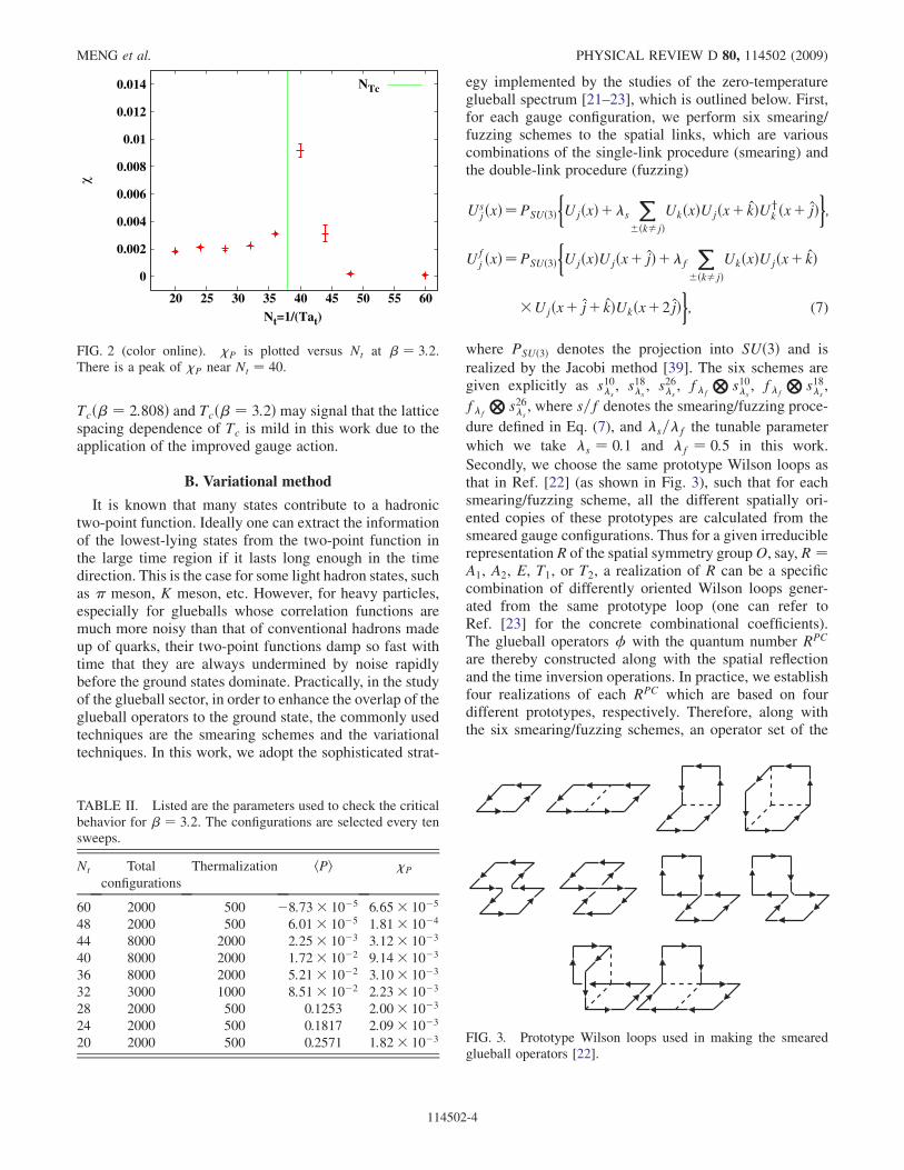
Tcð� ¼ 2:808Þ and Tcð� ¼ 3:2Þ may signal that the latticespacing dependence of Tc is mild in this work due to theapplication of the improved gauge action.

B. Variational method

It is known that many states contribute to a hadronictwo-point function. Ideally one can extract the informationof the lowest-lying states from the two-point function inthe large time region if it lasts long enough in the timedirection. This is the case for some light hadron states, suchas � meson, K meson, etc. However, for heavy particles,especially for glueballs whose correlation functions aremuch more noisy than that of conventional hadrons madeup of quarks, their two-point functions damp so fast withtime that they are always undermined by noise rapidlybefore the ground states dominate. Practically, in the studyof the glueball sector, in order to enhance the overlap of theglueball operators to the ground state, the commonly usedtechniques are the smearing schemes and the variationaltechniques. In this work, we adopt the sophisticated strat-

egy implemented by the studies of the zero-temperatureglueball spectrum [21–23], which is outlined below. First,for each gauge configuration, we perform six smearing/fuzzing schemes to the spatial links, which are variouscombinations of the single-link procedure (smearing) andthe double-link procedure (fuzzing)

UsjðxÞ¼PSUð3Þ

�UjðxÞþ�s

X�ðk�jÞ

UkðxÞUjðxþ kÞUyk ðxþ jÞ

�;

Ufj ðxÞ¼PSUð3Þ

�UjðxÞUjðxþ jÞþ�f

X�ðk�jÞ

UkðxÞUjðxþ kÞ

�Ujðxþ jþ kÞUkðxþ2jÞ�; (7)

where PSUð3Þ denotes the projection into SUð3Þ and is

realized by the Jacobi method [39]. The six schemes aregiven explicitly as s10�s

, s18�s, s26�s

, f�f

Ns10�s

, f�f

Ns18�s

,

f�f

Ns26�s

, where s=f denotes the smearing/fuzzing proce-

dure defined in Eq. (7), and �s=�f the tunable parameter

which we take �s ¼ 0:1 and �f ¼ 0:5 in this work.

Secondly, we choose the same prototype Wilson loops asthat in Ref. [22] (as shown in Fig. 3), such that for eachsmearing/fuzzing scheme, all the different spatially ori-ented copies of these prototypes are calculated from thesmeared gauge configurations. Thus for a given irreduciblerepresentationR of the spatial symmetry groupO, say, R ¼A1, A2, E, T1, or T2, a realization of R can be a specificcombination of differently oriented Wilson loops gener-ated from the same prototype loop (one can refer toRef. [23] for the concrete combinational coefficients).The glueball operators � with the quantum number RPC

are thereby constructed along with the spatial reflectionand the time inversion operations. In practice, we establishfour realizations of each RPC which are based on fourdifferent prototypes, respectively. Therefore, along withthe six smearing/fuzzing schemes, an operator set of the

TABLE II. Listed are the parameters used to check the criticalbehavior for � ¼ 3:2. The configurations are selected every tensweeps.

Nt Total

configurations

Thermalization hPi �P

60 2000 500 �8:73� 10�5 6:65� 10�5

48 2000 500 6:01� 10�5 1:81� 10�4

44 8000 2000 2:25� 10�3 3:12� 10�3

40 8000 2000 1:72� 10�2 9:14� 10�3

36 8000 2000 5:21� 10�2 3:10� 10�3

32 3000 1000 8:51� 10�2 2:23� 10�3

28 2000 500 0.1253 2:00� 10�3

24 2000 500 0.1817 2:09� 10�3

20 2000 500 0.2571 1:82� 10�3 FIG. 3. Prototype Wilson loops used in making the smearedglueball operators [22].

0

0.002

0.004

0.006

0.008

0.01

0.012

0.014

20 25 30 35 40 45 50 55 60

χ

Nt=1/(Tat)

NTc

FIG. 2 (color online). �P is plotted versus Nt at � ¼ 3:2.There is a peak of �P near Nt ¼ 40.

MENG et al. PHYSICAL REVIEW D 80, 114502 (2009)

114502-4

same specific quantum number RPC is composed of 24different operators, f�; ¼ 1; 2; . . . ; 24g. The last stepis the implementation of the variational method (VM).The main goal of VM is to find an optimal combinationof the set of operators,� ¼ P

v�, which overlaps mostto a specific state (in this work, we only focus on theground states). The combinational coefficients v ¼fv; ¼ 1; 2; . . . ; ng can be obtained by minimizing theeffective mass,

~mðtDÞ ¼ � 1

tDln

P�

vv�~C�ðtDÞP

�

vv�~C�ð0Þ

; (8)

at tD ¼ 1, where ~C�ðtÞ is the correlation matrix of the

operator set,

~C�ðtÞ ¼X

h0j�ðtþ Þ��ðÞj0i: (9)

This is equivalent to solving the generalized eigenvalueequation

~CðtDÞvðRÞ ¼ e�tD ~mðtDÞ ~Cð0ÞvðRÞ; (10)

and the eigenvector v gives the desired combinationalcoefficients. Thus, the optimal operator that couples mostto a specific state (the ground state in this work) can bebuilt up as

� ¼ X

v�; (11)

whose correlator CðtÞ is expected to be dominated by thecontribution of this state.

III. DATA ANALYSIS OF THE THERMALCORRELATORS OF GLUEBALLS

All 20 RPC channels, with R ¼ A1; A2; E; T1; T2 andPC ¼ þþ;þ�;�þ;�� , are considered in the calcula-tion of the thermal correlators of glueballs on anisotropiclattices mentioned in Sec. II. At each temperature, after10 000 pseudo-heat-bath sweeps of thermalization, themeasurements are carried out every three compoundsweeps, with each compound sweep composed of onepseudo-heat-bath and five microcanonical overrelaxationsweeps. In order to reduce the possible autocorrelations,the measured data are divided into bins of the size nmb ¼400, and each bin is regarded as an independent measure-ment in the data analysis procedure. The numbers of binsNbin and nmb at various temperatures are listed in Table III.

Theoretically, under the periodic boundary condition inthe temporal direction, the temporal correlators Cðt; TÞ atthe temperature T can be written in the spectral represen-tation as

Cðt; TÞ � 1

ZðTÞ Trðe�H=T�ðtÞ�ð0ÞÞ

¼ Xm;n

jhnj�jmij22ZðTÞ exp

��Em þ En

2T

�

� cosh

��t� 1

2T

�ðEn � EmÞ

�

¼Z 1

�1d!�ð!ÞKð!; TÞ; (12)

with a T-dependent kernel

Kð!;TÞ ¼ coshð!=ð2TÞ �!tÞsinhð!=ð2TÞÞ (13)

and the spectral function,

�ð!Þ ¼ Xm;n

jhnj�jmij22ZðTÞ e�Em=Tð�ð!� ðEn � EmÞ

� �ð!� ðEm � EnÞÞ; (14)

where ZðTÞ is the partition function at T, and En the energyof the thermal state jni (j0i represents the vacuum state). Inthe zero-temperature limit (T ! 0), due to the factorexpð�Em=TÞ, the spectral function �ð!Þ degenerates to

�ð!Þ ¼ Xn

jh0j�jnij22Zð0Þ ð�ð!� EnÞ � �ð!þ EnÞÞ; (15)

thus we have the function form of the correlation function,

Cðt; T ¼ 0Þ ¼ Xn

Wne�En (16)

with Wn ¼ jh0j�jnij2=Zð0Þ.However, for any finite temperature (this is always the

case for finite lattices), all the thermal states with thenonzero matrix elements hmj�jni may contribute to thespectral function �ð!Þ. Intuitively in the confinementphase, the fundamental degrees of freedom are hadronlikemodes; thus the thermal states should be multihadron

TABLE III. Simulation parameters to calculate glueball spec-trum. � ¼ 3:2, as ¼ 0:0878 fm, Ls ¼ 2:11 fm.

Nt T=Tc nmb Nbin

128 0.30 400 24

80 0.47 400 30

60 0.63 400 44

48 0.79 400 40

44 0.86 400 44

40 0.95 400 40

36 1.05 400 40

32 1.19 400 56

28 1.36 400 40

24 1.58 400 40

20 1.90 400 40

GLUEBALLS AT FINITE TEMPERATURE IN SUð3Þ . . . PHYSICAL REVIEW D 80, 114502 (2009)

114502-5

states. If they interact weakly with each other, we can treatthem as free particles at the lowest order approximationand consider Em as the sum of the energies of hadronsincluding in the thermal state jmi. Since the contribution ofa thermal state jmi to the spectral function is weighted bythe factor expð�Em=TÞ, apart from the vacuum state, themaximal value of this factor is expð�Mmin=TÞ with Mmin

the mass of the lightest hadron mode in the system. As faras the quenched glueball system is concerned, the lightestglueball is the scalar, whose mass at the low temperature isroughly M0þþ � 1:6 GeV, which gives a very tiny weightfactor expð�M0þþ=TcÞ � 0:003 at Tc in comparison withunity factor of the vacuum state. That is to say, for thequenched glueballs, up to the critical temperature Tc, thecontributions of higher spectral components beyond thevacuum to the spectral function are much smaller than thestatistical errors (the relative statistical errors of the ther-mal glueball correlators are always a few percent) and canbe neglected. As a result, the function form of �ð!Þ in

Eq. (15) can be a good approximation for the spectralfunction of glueballs at least up to Tc. Accordingly, con-sidering the finite extension of the lattice in the temporaldirection, the function form of the thermal correlators canbe approximated as

Cðt; TÞ ¼ Xn

Wn

coshðMnð1=ð2TÞ � tÞÞsinhðMn=ð2TÞÞ ; (17)

which is surely the commonly used function form for thestudy of hadron masses at low temperatures on the lattice.As is always done, the glueball masses Mn derived by thisfunction are called the pole masses in this work.

A. Results of the single-cosh fit

Even though the above discussions are based on theweak-interaction approximation for the hadronlike modesbelow Tc, we would like to apply Eq. (17) to analyzing thethermal correlators all over the temperature in concern.

0

0.05

0.1

0.15

0.2

0.25

0.3

0 5 10 15 20 25 30

Ma t

t

Meff(Nt=128)

0

0.05

0.1

0.15

0.2

0.25

0.3

0 5 10 15 20 25

Ma t

t

Meff(Nt=60)

0

0.05

0.1

0.15

0.2

0.25

0.3

0 2 4 6 8 10 12 14 16 18

Ma t

t

Meff(Nt=40)

0

0.05

0.1

0.15

0.2

0.25

0.3

0 2 4 6 8 10 12 14 16 18

Ma t

t

Meff(Nt=36)

0

0.05

0.1

0.15

0.2

0.25

0.3

0 2 4 6 8 10 12

Ma t

t

Meff(Nt=24)

0

0.05

0.1

0.15

0.2

0.25

0.3

0 2 4 6 8 10

Ma t

t

Meff(Nt=20)

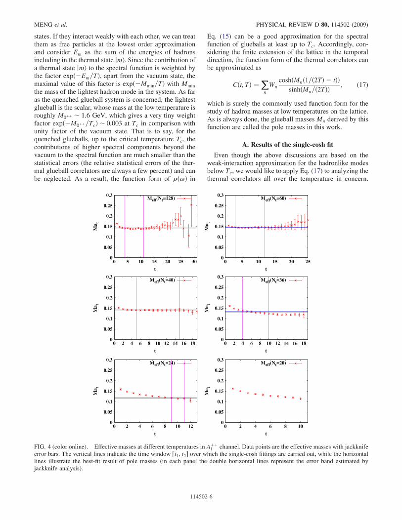
FIG. 4 (color online). Effective masses at different temperatures in Aþþ1 channel. Data points are the effective masses with jackknife

error bars. The vertical lines indicate the time window ½t1; t2� over which the single-cosh fittings are carried out, while the horizontallines illustrate the best-fit result of pole masses (in each panel the double horizontal lines represent the error band estimated byjackknife analysis).

MENG et al. PHYSICAL REVIEW D 80, 114502 (2009)

114502-6

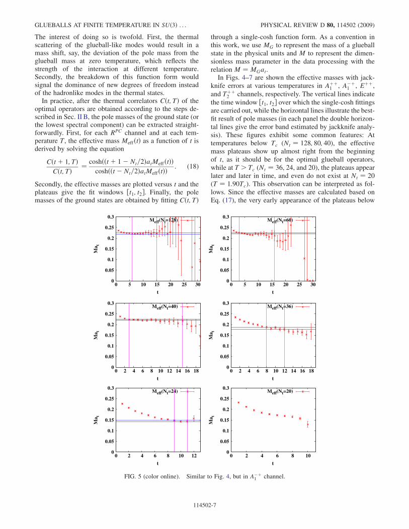
The interest of doing so is twofold. First, the thermalscattering of the glueball-like modes would result in amass shift, say, the deviation of the pole mass from theglueball mass at zero temperature, which reflects thestrength of the interaction at different temperature.Secondly, the breakdown of this function form wouldsignal the dominance of new degrees of freedom insteadof the hadronlike modes in the thermal states.

In practice, after the thermal correlators Cðt; TÞ of theoptimal operators are obtained according to the steps de-scribed in Sec. II B, the pole masses of the ground state (orthe lowest spectral component) can be extracted straight-forwardly. First, for each RPC channel and at each tem-perature T, the effective mass MeffðtÞ as a function of t isderived by solving the equation

Cðtþ 1; TÞCðt; TÞ ¼ coshððtþ 1� Nt=2ÞatMeffðtÞÞ

coshððt� Nt=2ÞatMeffðtÞÞ : (18)

Secondly, the effective masses are plotted versus t and theplateaus give the fit windows ½t1; t2�. Finally, the polemasses of the ground states are obtained by fitting Cðt; TÞ

through a single-cosh function form. As a convention inthis work, we use MG to represent the mass of a glueballstate in the physical units and M to represent the dimen-sionless mass parameter in the data processing with therelation M ¼ MGat.In Figs. 4–7 are shown the effective masses with jack-

knife errors at various temperatures in Aþþ1 , A�þ

1 , Eþþ,and Tþþ

2 channels, respectively. The vertical lines indicate

the time window ½t1; t2� over which the single-cosh fittingsare carried out, while the horizontal lines illustrate the best-fit result of pole masses (in each panel the double horizon-tal lines give the error band estimated by jackknife analy-sis). These figures exhibit some common features: Attemperatures below Tc (Nt ¼ 128; 80; 40), the effectivemass plateaus show up almost right from the beginningof t, as it should be for the optimal glueball operators,while at T > Tc (Nt ¼ 36, 24, and 20), the plateaus appearlater and later in time, and even do not exist at Nt ¼ 20(T ¼ 1:90Tc). This observation can be interpreted as fol-lows. Since the effective masses are calculated based onEq. (17), the very early appearance of the plateaus below

0

0.05

0.1

0.15

0.2

0.25

0.3

0 5 10 15 20 25 30

Ma t

t

Meff(Nt=128)

0

0.05

0.1

0.15

0.2

0.25

0.3

0 5 10 15 20 25 30

Ma t

t

Meff(Nt=60)

0

0.05

0.1

0.15

0.2

0.25

0.3

0 2 4 6 8 10 12 14 16 18

Ma t

t

Meff(Nt=40)

0

0.05

0.1

0.15

0.2

0.25

0.3

0 2 4 6 8 10 12 14 16 18

Ma t

t

Meff(Nt=36)

0

0.05

0.1

0.15

0.2

0.25

0.3

0 2 4 6 8 10 12

Ma t

t

Meff(Nt=24)

0

0.05

0.1

0.15

0.2

0.25

0.3

0 2 4 6 8 10

Ma t

t

Meff(Nt=20)

FIG. 5 (color online). Similar to Fig. 4, but in A�þ1 channel.

GLUEBALLS AT FINITE TEMPERATURE IN SUð3Þ . . . PHYSICAL REVIEW D 80, 114502 (2009)

114502-7

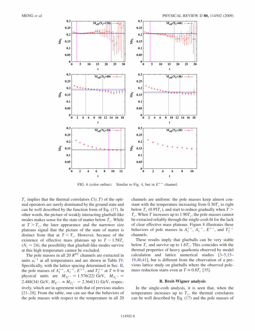
Tc implies that the thermal correlators Cðt; TÞ of the opti-mal operators are surely dominated by the ground state andcan be well described by the function form of Eq. (17). Inother words, the picture of weakly interacting glueball-likemodes makes sense for the state of matter below Tc. Whileat T > Tc, the later appearance and the narrower sizeplateaus signal that the picture of the state of matter isdistinct from that at T < Tc. However, because of theexistence of effective mass plateaus up to T � 1:58Tc

(Nt ¼ 24), the possibility that glueball-like modes surviveat this high temperature cannot be excluded.

The pole masses in all 20 RPC channels are extracted inunits a�1

t at all temperatures and are shown in Table IV.Specifically, with the lattice spacing determined in Sec. II,the pole masses of Aþþ

1 , A�þ1 , Eþþ, and Tþþ

2 at T ’ 0 in

physical units are MAþþ1

¼ 1:576ð22Þ GeV, MA�þ1

¼2:488ð34Þ GeV, MEþþ ’ MTþþ

2¼ 2:364ð11Þ GeV, respec-

tively, which are in agreement with that of previous studies[21–28]. From the table, one can see that the behaviors ofthe pole masses with respect to the temperature in all 20

channels are uniform: the pole masses keep almost con-stant with the temperature increasing from 0:30Tc to rightbelow Tc (0:95Tc), and start to reduce gradually when T >Tc. When T increases up to 1:90Tc, the pole masses cannotbe extracted reliably through the single-cosh fit for the lackof clear effective mass plateaus. Figure 8 illustrates thesebehaviors of pole masses in Aþþ

1 , A�þ1 , Eþþ, and Tþþ

2

channels.These results imply that glueballs can be very stable

below Tc and survive up to 1:6Tc. This coincides with thethermal properties of heavy quarkonia observed by modelcalculation and lattice numerical studies [3–5,15–19,40,41], but is different from the observation of a pre-vious lattice study on glueballs where the observed pole-mass reduction starts even at T ’ 0:8Tc [35].

B. Breit-Wigner analysis

In the single-cosh analysis, it is seen that, when thetemperature increases up to Tc, the thermal correlatorscan be well described by Eq. (17) and the pole masses of

0

0.05

0.1

0.15

0.2

0.25

0.3

0 5 10 15 20 25 30M

a t

t

Meff(Nt=128)

0

0.05

0.1

0.15

0.2

0.25

0.3

0 5 10 15 20 25 30

Ma t

t

Meff(Nt=60)

0

0.05

0.1

0.15

0.2

0.25

0.3

0 2 4 6 8 10 12 14 16 18

Ma t

t

Meff(Nt=40)

0

0.05

0.1

0.15

0.2

0.25

0.3

0 2 4 6 8 10 12 14 16 18

Ma t

t

Meff(Nt=36)

0

0.05

0.1

0.15

0.2

0.25

0.3

0 2 4 6 8 10 12

Ma t

t

Meff(Nt=24)

0

0.05

0.1

0.15

0.2

0.25

0.3

0 2 4 6 8 10

Ma t

t

Meff(Nt=20)

FIG. 6 (color online). Similar to Fig. 4, but in Eþþ channel.

MENG et al. PHYSICAL REVIEW D 80, 114502 (2009)

114502-8

0

0.05

0.1

0.15

0.2

0.25

0.3

0 5 10 15 20 25 30M

a t

t

Meff(Nt=128)

0

0.05

0.1

0.15

0.2

0.25

0.3

0 5 10 15 20 25 30

Ma t

t

Meff(Nt=60)

0

0.05

0.1

0.15

0.2

0.25

0.3

0 2 4 6 8 10 12 14 16 18

Ma t

t

Meff(Nt=40)

0

0.05

0.1

0.15

0.2

0.25

0.3

0 2 4 6 8 10 12 14 16 18

Ma t

t

Meff(Nt=36)

0

0.05

0.1

0.15

0.2

0.25

0.3

0 2 4 6 8 10 12

Ma t

t

Meff(Nt=24)

0

0.05

0.1

0.15

0.2

0.25

0.3

0 2 4 6 8 10

Ma t

t

Meff(Nt=20)

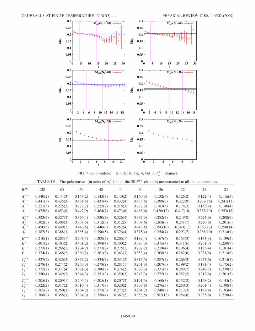
FIG. 7 (color online). Similar to Fig. 4, but in Tþþ2 channel.

TABLE IV. The pole masses (in units of a�1t ) in all the 20 RPC channels are extracted at all the temperatures.

RPC 128 80 60 48 44 40 36 32 28 24

Aþþ1 0.140(2) 0.144(3) 0.144(2) 0.143(3) 0.140(2) 0.140(3) 0.132(4) 0.126(2) 0.122(4) 0.116(3)

Aþ�1 0.441(3) 0.435(3) 0.434(5) 0.437(4) 0.432(4) 0.435(5) 0.399(6) 0.322(9) 0.267(16) 0.241(13)

A�þ1 0.221(3) 0.225(2) 0.222(2) 0.225(2) 0.218(3) 0.222(2) 0.183(5) 0.174(3) 0.155(4) 0.146(4)

A��1 0.475(6) 0.453(8) 0.447(9) 0.464(7) 0.473(6) 0.468(6) 0.426(12) 0.417(10) 0.287(19) 0.253(18)

Aþþ2 0.323(4) 0.327(4) 0.326(4) 0.330(2) 0.326(4) 0.332(3) 0.282(7) 0.249(8) 0.224(9) 0.208(9)

Aþ�2 0.302(5) 0.308(3) 0.308(5) 0.312(3) 0.312(5) 0.308(6) 0.268(6) 0.241(7) 0.220(8) 0.201(6)

A�þ2 0.450(5) 0.449(7) 0.446(5) 0.440(6) 0.452(4) 0.448(5) 0.396(10) 0.340(11) 0.330(12) 0.250(14)

A��2 0.387(3) 0.388(3) 0.385(4) 0.390(5) 0.376(4) 0.375(4) 0.354(7) 0.293(7) 0.268(10) 0.214(9)

Eþþ 0.210(1) 0.205(1) 0.207(1) 0.209(2) 0.206(1) 0.189(4) 0.167(4) 0.153(3) 0.143(3) 0.139(2)

Eþ� 0.401(2) 0.403(2) 0.401(2) 0.394(4) 0.400(2) 0.395(3) 0.375(4) 0.311(6) 0.261(7) 0.230(7)

E�þ 0.273(1) 0.266(1) 0.264(2) 0.273(2) 0.275(1) 0.262(2) 0.218(4) 0.196(4) 0.183(4) 0.181(4)

E�� 0.374(1) 0.368(2) 0.360(2) 0.361(3) 0.363(3) 0.352(4) 0.308(8) 0.262(6) 0.231(6) 0.213(6)

Tþþ1 0.327(2) 0.326(4) 0.327(2) 0.334(2) 0.331(2) 0.312(5) 0.287(7) 0.266(3) 0.227(6) 0.215(4)

Tþ�1 0.278(1) 0.274(2) 0.265(3) 0.278(2) 0.281(1) 0.261(3) 0.207(6) 0.199(2) 0.181(4) 0.175(2)

T�þ1 0.372(2) 0.377(4) 0.371(3) 0.380(2) 0.374(2) 0.370(3) 0.331(5) 0.289(7) 0.248(7) 0.230(5)

T��1 0.350(4) 0.349(2) 0.344(3) 0.351(2) 0.350(2) 0.343(3) 0.272(8) 0.252(5) 0.212(6) 0.201(5)

Tþþ2 0.205(1) 0.209(1) 0.206(1) 0.205(1) 0.207(2) 0.191(3) 0.160(3) 0.152(2) 0.148(2) 0.143(2)

Tþ�1 0.322(2) 0.317(2) 0.310(4) 0.317(3) 0.320(2) 0.303(5) 0.276(5) 0.250(3) 0.201(4) 0.190(4)

T�þ1 0.265(2) 0.260(3) 0.264(2) 0.273(3) 0.272(2) 0.264(2) 0.240(3) 0.213(3) 0.187(4) 0.183(4)

T��1 0.368(2) 0.358(3) 0.364(3) 0.358(4) 0.367(2) 0.353(5) 0.282(13) 0.254(6) 0.235(6) 0.220(4)

GLUEBALLS AT FINITE TEMPERATURE IN SUð3Þ . . . PHYSICAL REVIEW D 80, 114502 (2009)

114502-9

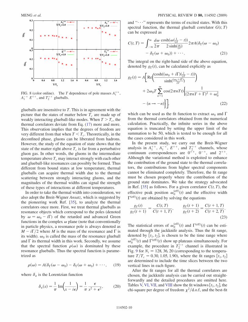
glueballs are insensitive to T. This is in agreement with thepicture that the states of matter below Tc are made up ofweakly interacting glueball-like modes. When T > Tc, thethermal correlators deviate from Eq. (17) more and more.This observation implies that the degrees of freedom arevery different from that when T < Tc. Theoretically, in thedeconfined phase, gluons can be liberated from hadrons.However, the study of the equation of state shows that thestate of the matter right above Tc is far from a perturbativegluon gas. In other words, the gluons in the intermediatetemperature above Tc may interact strongly with each otherand glueball-like resonances can possibly be formed. Thusdifferent from bound states at low temperature, thermalglueballs can acquire thermal width due to the thermalscattering between strongly interacting gluons, and themagnitudes of the thermal widths can signal the strengthof these types of interactions at different temperatures.

In order to take the thermal width into consideration, wealso adopt the Breit-Wigner Ansatz, which is suggested bythe pioneering work Ref. [35], to analyze the thermalcorrelators once more. First, we treat thermal glueballs asresonance objects which correspond to the poles (denotedby ! ¼ !0 � i�) of the retarded and advanced Greenfunctions in the complex! plane (note that conventionallyin particle physics, a resonance pole is always denoted asM� i�=2 where M is the mass of the resonance and � isits width). !0 is called the mass of the resonance glueballand � its thermal width in this work. Secondly, we assumethat the spectral function �ð!Þ is dominated by theseresonance glueballs. Thus the spectral function is parame-trized as

�ð!Þ ¼ Að��ð!�!0Þ � ��ð!þ!0Þ þ ; (19)

where � is the Lorentzian function

� ðxÞ ¼ 1

�Im

�1

x� i

�¼ 1

�

x2 þ 2; (20)

and ‘‘ ’’ represents the terms of excited states. With thisspectral function, the thermal glueball correlator Gðt; TÞcan be expressed as

Cðt; TÞ ¼Z 1

�1d!

2�

coshð!ð 12T � tÞÞ2 sinhð!2TÞ

2�Að��ð!�!0Þ

� ��ð!þ!0ÞÞ þ : (21)

The integral on the right-hand side of the above equation,denoted by g�ðtÞ, can be calculated explicitly as

g�ðtÞ ¼ A

�Re

�coshðð!0 þ i�Þð 12T � tÞÞ

sinhðð!0þi�Þ2T Þ

�

þ 2!0TX1n¼1

cosð2�nTtÞ�

1

ð2�nT þ �Þ2 þ!20

� ðn ! �nÞ��; (22)

which can be used as the fit function to extract !0 and �from the thermal correlators obtained from the numericalcalculation. Practically, the infinite series in the aboveequation is truncated by setting the upper limit of thesummation to be 50, which is tested to be enough for allthe cases considered in this work.In the present study, we carry out the Breit-Wigner

analysis in Aþþ1 , A�þ

1 , Eþþ, and Tþþ2 channels, whose

continuum correspondences are 0þþ, 0�þ, and 2þþ.Although the variational method is exploited to enhancethe contribution of the ground state to the thermal correla-tors, the contributions from higher spectral componentscannot be eliminated completely. Therefore, the fit rangemust be chosen properly where the contribution of theground state dominates. We take the strategy advocatedin Ref. [35] as follows. For a given correlator Cðt; TÞ, theeffective peak position !ðeffÞ

0 ðtÞ and the effective width

�ðeffÞðtÞ are obtained by solving the equations

g�ðtÞg�ðtþ 1Þ ¼ Cðt; TÞ

Cðtþ 1; TÞ ;g�ðtþ 1Þg�ðtþ 2Þ ¼

Cðtþ 1; TÞCðtþ 2; TÞ :

(23)

The statistical errors of !ðeffÞ0 ðtÞ and �ðeffÞðtÞ can be esti-

mated through the jackknife analysis. Thus the fit range,denoted by ½t1; t2�, is chosen to be the time range where

!ðeffÞ0 ðtÞ and �ðeffÞðtÞ show up plateaus simultaneously. For

example, the procedure in Tþþ2 channel is illustrated in

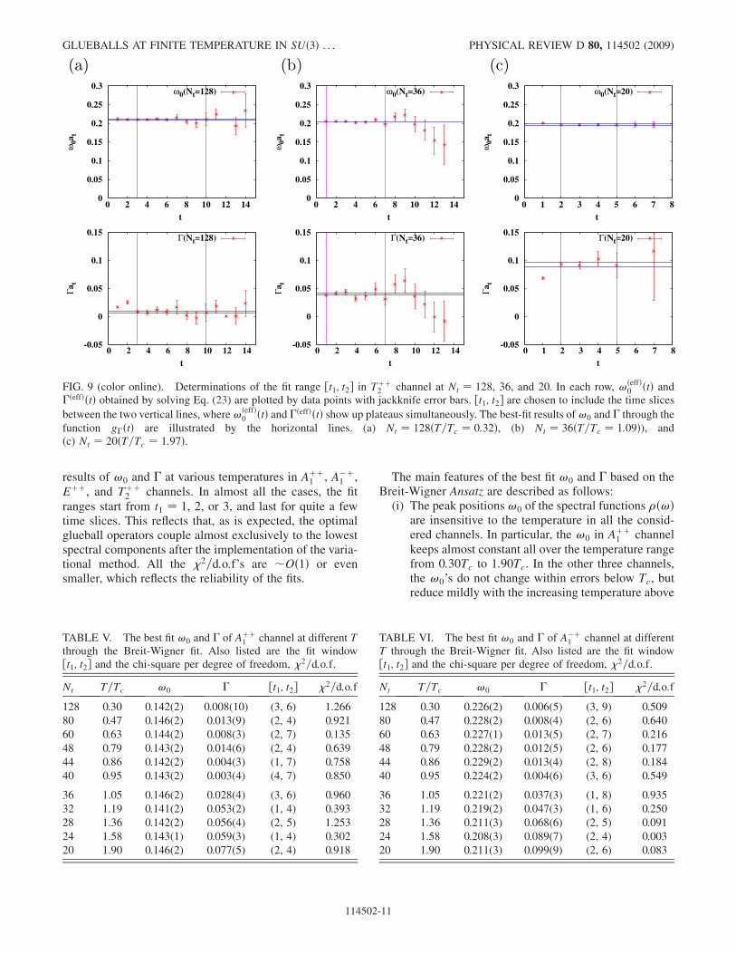
Fig. 9 for Nt ¼ 128; 36; 20 (corresponding to the tempera-ture T=Tc ¼ 0:30; 1:05; 1:90), where the fit ranges ½t1; t2�are determined to include the time slices between the twovertical lines in each figure.After the fit ranges for all the thermal correlators are

chosen, the jackknife analysis can be carried out straight-forwardly and the detailed procedures are omitted here.Tables V, VI, VII, and VIII show the fit windows ½t1; t2�, thechi-square per degree of freedom �2=d:o:f, and the best-fit

0

0.1

0.2

0.3M

a tA1

++

T/Tc=1.0A1

-+

T/Tc=1.0

0

0.1

0.2

0.3

0 0.4 0.8 1.2 1.6

Ma t

T/Tc

E++

T/Tc=1.0

0 0.4 0.8 1.2 1.6

T/Tc

T2++

T/Tc=1.0

FIG. 8 (color online). The T dependence of pole masses Aþþ1 ,

A�þ1 Eþþ, and Tþþ

2 glueballs.

MENG et al. PHYSICAL REVIEW D 80, 114502 (2009)

114502-10

results of !0 and � at various temperatures in Aþþ1 , A�þ

1 ,Eþþ, and Tþþ

2 channels. In almost all the cases, the fitranges start from t1 ¼ 1, 2, or 3, and last for quite a fewtime slices. This reflects that, as is expected, the optimalglueball operators couple almost exclusively to the lowestspectral components after the implementation of the varia-tional method. All the �2=d:o:f’s are �Oð1Þ or evensmaller, which reflects the reliability of the fits.

The main features of the best fit !0 and � based on theBreit-Wigner Ansatz are described as follows:(i) The peak positions!0 of the spectral functions �ð!Þ

are insensitive to the temperature in all the consid-ered channels. In particular, the !0 in Aþþ

1 channelkeeps almost constant all over the temperature rangefrom 0:30Tc to 1:90Tc. In the other three channels,the !0’s do not change within errors below Tc, butreduce mildly with the increasing temperature above

TABLE VI. The best fit !0 and � of A�þ1 channel at different

T through the Breit-Wigner fit. Also listed are the fit window½t1; t2� and the chi-square per degree of freedom, �2=d:o:f.

Nt T=Tc !0 � ½t1; t2� �2=d:o:f

128 0.30 0.226(2) 0.006(5) (3, 9) 0.509

80 0.47 0.228(2) 0.008(4) (2, 6) 0.640

60 0.63 0.227(1) 0.013(5) (2, 7) 0.216

48 0.79 0.228(2) 0.012(5) (2, 6) 0.177

44 0.86 0.229(2) 0.013(4) (2, 8) 0.184

40 0.95 0.224(2) 0.004(6) (3, 6) 0.549

36 1.05 0.221(2) 0.037(3) (1, 8) 0.935

32 1.19 0.219(2) 0.047(3) (1, 6) 0.250

28 1.36 0.211(3) 0.068(6) (2, 5) 0.091

24 1.58 0.208(3) 0.089(7) (2, 4) 0.003

20 1.90 0.211(3) 0.099(9) (2, 6) 0.083

0

0.05

0.1

0.15

0.2

0.25

0.3

0 2 4 6 8 10 12 14

ω0a

t

t

ω0(Nt=128)

0

0.05

0.1

0.15

0.2

0.25

0.3

0 2 4 6 8 10 12 14

ω0a

t

t

ω0(Nt=36)

0

0.05

0.1

0.15

0.2

0.25

0.3

0 1 2 3 4 5 6 7 8

ω0a

t

t

ω0(Nt=20)

-0.05

0

0.05

0.1

0.15

0 2 4 6 8 10 12 14

Γat

t

Γ(Nt=128)

-0.05

0

0.05

0.1

0.15

0 2 4 6 8 10 12 14

Γat

t

Γ(Nt=36)

-0.05

0

0.05

0.1

0.15

0 1 2 3 4 5 6 7 8

Γat

t

Γ(Nt=20)

FIG. 9 (color online). Determinations of the fit range ½t1; t2� in Tþþ2 channel at Nt ¼ 128, 36, and 20. In each row, !ðeffÞ

0 ðtÞ and�ðeffÞðtÞ obtained by solving Eq. (23) are plotted by data points with jackknife error bars. ½t1; t2� are chosen to include the time slices

between the two vertical lines, where!ðeffÞ0 ðtÞ and �ðeffÞðtÞ show up plateaus simultaneously. The best-fit results of!0 and � through the

function g�ðtÞ are illustrated by the horizontal lines. (a) Nt ¼ 128ðT=Tc ¼ 0:32Þ, (b) Nt ¼ 36ðT=Tc ¼ 1:09Þ), and(c) Nt ¼ 20ðT=Tc ¼ 1:97Þ.

TABLE V. The best fit !0 and � of Aþþ1 channel at different T

through the Breit-Wigner fit. Also listed are the fit window½t1; t2� and the chi-square per degree of freedom, �2=d:o:f.

Nt T=Tc !0 � ½t1; t2� �2=d:o:f

128 0.30 0.142(2) 0.008(10) (3, 6) 1.266

80 0.47 0.146(2) 0.013(9) (2, 4) 0.921

60 0.63 0.144(2) 0.008(3) (2, 7) 0.135

48 0.79 0.143(2) 0.014(6) (2, 4) 0.639

44 0.86 0.142(2) 0.004(3) (1, 7) 0.758

40 0.95 0.143(2) 0.003(4) (4, 7) 0.850

36 1.05 0.146(2) 0.028(4) (3, 6) 0.960

32 1.19 0.141(2) 0.053(2) (1, 4) 0.393

28 1.36 0.142(2) 0.056(4) (2, 5) 1.253

24 1.58 0.143(1) 0.059(3) (1, 4) 0.302

20 1.90 0.146(2) 0.077(5) (2, 4) 0.918

GLUEBALLS AT FINITE TEMPERATURE IN SUð3Þ . . . PHYSICAL REVIEW D 80, 114502 (2009)

114502-11

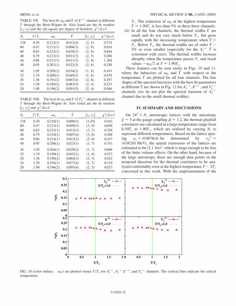
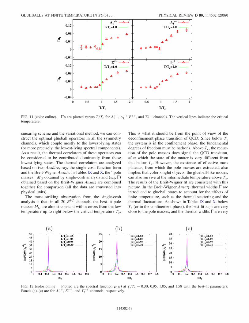
Tc. The reduction of !0 at the highest temperatureT ¼ 1:90Tc is less than 5% in these three channels.

(ii) In all the four channels, the thermal widths � aresmall and do not vary much below Tc, but growrapidly with the increasing temperature when T >Tc. Below Tc, the thermal widths are of order ��5% or even smaller (especially for the Aþþ

1 � is

consistent with zero). The thermal widths increaseabruptly when the temperature passes Tc and reachvalues �!0=2 at T ¼ 1:90Tc.

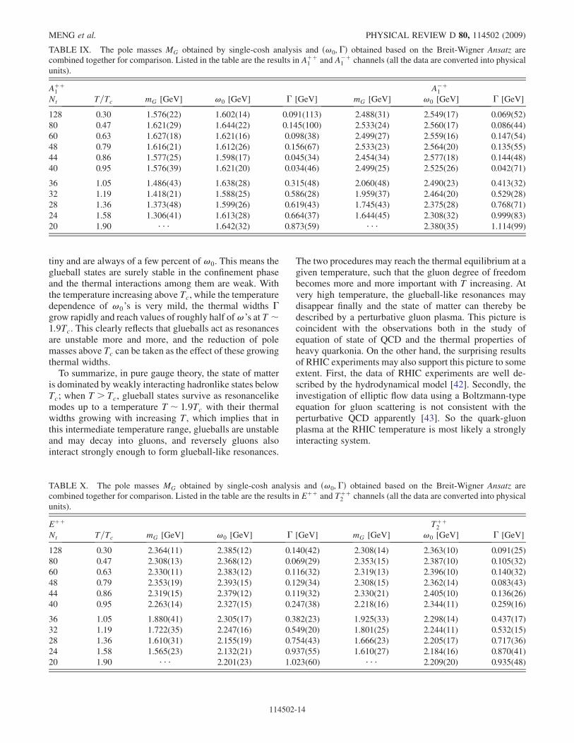
These features can be seen easily in Figs. 10 and 11,where the behaviors of !0 and � with respect to thetemperature T are plotted for all four channels. The lineshapes of the spectral functions with the best-fit parametersat different T are shown in Fig. 12 for A�þ

1 , Eþþ, and Tþþ2

channels (we do not plot the spectral function of Aþþ1

channel due to the small thermal widths).

IV. SUMMARYAND DISCUSSIONS

On 243 � Nt anisotropic lattices with the anisotropy� ¼ 5 at the gauge coupling � ¼ 3:2, the thermal glueballcorrelators are calculated in a large temperature range from0:30Tc to 1:90Tc, which are realized by varying Nt torepresent different temperatures. Based on the lattice spac-ing as ¼ 0:0878ð4Þ fm determined by r�1

0 ¼ð410ð20Þ MeVÞ, the spatial extensions of the lattices areestimated to be ð2:1 fmÞ3, which is large enough to be freeof the finite volume effects. On the other hand, because ofthe large anisotropy, there are enough data points in thetemporal direction for the thermal correlators to be ana-lyzed comfortably even at the highest temperature T � 2Tc

concerned in this work. With the implementation of the

TABLE VII. The best-fit !0 and � of Eþþ channel at differentT through the Breit-Wigner fit. Also listed are the fit window½t1; t2� and the chi-square per degree of freedom, �2=d:o:f.

Nt T=Tc !0 � ½t1; t2� �2=d:o:f:

128 0.30 0.212(1) 0.012(4) (2, 5) 0.274

80 0.47 0.211(1) 0.006(3) (2, 8) 0.616

60 0.63 0.212(1) 0.010(3) (2, 9) 0.844

48 0.79 0.213(1) 0.011(3) (2, 5) 0.206

44 0.86 0.211(1) 0.011(3) (2, 8) 1.268

40 0.95 0.207(1) 0.022(3) (2, 6) 0.250

36 1.05 0.205(2) 0.034(2) (1, 8) 0.183

32 1.19 0.200(1) 0.049(2) (1, 6) 0.478

28 1.36 0.191(2) 0.067(4) (2, 6) 0.297

24 1.58 0.189(2) 0.083(5) (2, 4) 0.253

20 1.90 0.196(2) 0.091(5) (2, 4) 0.046

TABLE VIII. The best fit!0 and � of Tþþ2 channel at different

T through the Breit-Wigner fit. Also listed are the fit window½t1; t2� and �2=d:o:f.

Nt T=Tc !0 � ½t1; t2� �2=d:o:f

128 0.30 0.210(1) 0.008(2) (3,10) 0.442

80 0.47 0.213(1) 0.009(3) (3, 9) 0.696

60 0.63 0.213(1) 0.012(3) (3, 7) 0.326

48 0.79 0.210(1) 0.007(4) (3, 6) 0.288

44 0.86 0.214(1) 0.012(2) (2, 6) 0.437

40 0.95 0.208(1) 0.023(1) (1, 7) 0.743

36 1.05 0.204(1) 0.039(2) (1, 7) 0.606

32 1.19 0.199(1) 0.047(1) (1, 6) 0.527

28 1.36 0.196(2) 0.064(3) (2, 5) 0.022

24 1.58 0.194(1) 0.077(4) (2, 7) 0.119

20 1.90 0.196(2) 0.093(4) (2, 5) 0.027

0

0.05

0.1

0.15

0.2

0.25

0.3

ω0a

t

A1++

T/Tc=1.0A1

-+

T/Tc=1.0

0

0.05

0.1

0.15

0.2

0.25

0.3

0 0.5 1 1.5 2

ω0a

t

T/Tc

E++

T/Tc=1.0

0 0.5 1 1.5 2

T/Tc

T2++

T/Tc=1.0

FIG. 10 (color online). !0’s are plotted versus T=Tc for Aþþ1 , A�þ

1 Eþþ, and Tþþ2 channels. The vertical lines indicate the critical

temperature.

MENG et al. PHYSICAL REVIEW D 80, 114502 (2009)

114502-12

smearing scheme and the variational method, we can con-struct the optimal glueball operators in all the symmetrychannels, which couple mostly to the lowest-lying states(or more precisely, the lowest-lying spectral components).As a result, the thermal correlators of these operators canbe considered to be contributed dominantly from theselowest-lying states. The thermal correlators are analyzedbased on two Ansatze, say, the single-cosh function formand the Breit-Wigner Ansatz. In Tables IX and X, the ‘‘polemasses’’ MG obtained by single-cosh analysis and ð!0;�Þobtained based on the Breit-Wigner Ansatz are combinedtogether for comparison (all the data are converted intophysical units).

The most striking observation from the single-coshanalysis is that, in all 20 RPC channels, the best-fit polemasses MG are almost constant within errors from the lowtemperature up to right below the critical temperature Tc.

This is what it should be from the point of view of thedeconfinement phase transition of QCD: Since below Tc

the system is in the confinement phase, the fundamentaldegrees of freedom must be hadrons. Above Tc, the reduc-tion of the pole masses does signal the QCD transition,after which the state of the matter is very different fromthat below Tc. However, the existence of effective massplateaus, from which the pole masses are extracted, alsoimplies that color singlet objects, the glueball-like modes,can also survive at the intermediate temperature above Tc.The results of the Breit-Wigner fit are consistent with thispicture. In the Breit-Wigner Ansatz, thermal widths � areintroduced to glueball states to account for the effects offinite temperature, such as the thermal scattering and thethermal fluctuations. As shown in Tables IX and X, belowTc (or in the confinement phase), the best-fit !0’s are veryclose to the pole masses, and the thermal widths � are very

-0.04

0

0.04

0.08

0.12

Γat

A1++

T/Tc=1.0A1

-+

T/Tc=1.0

-0.04

0

0.04

0.08

0.12

0 0.5 1 1.5 2

Γat

T/Tc

E++

T/Tc=1.0

0 0.5 1 1.5 2

T/Tc

T2++

T/Tc=1.0

FIG. 11 (color online). �’s are plotted versus T=Tc for Aþþ1 , A�þ

1 Eþþ, and Tþþ2 channels. The vertical lines indicate the critical

temperature.

0 5

10 15 20 25 30 35 40 45 50

0 0.1 0.2 0.3 0.4 0.5 0.6 0.7 0.8

(ω)/

G(0

)[a t

-1]

ωat

T/Tc=1.58T/Tc=1.05T/Tc=0.95T/Tc=0.30

0

5

10

15

20

25

0 0.1 0.2 0.3 0.4 0.5 0.6 0.7 0.8

(ω)/

G(0

)[a t

-1]

ωat

T/Tc=1.58T/Tc=1.05T/Tc=0.95T/Tc=0.30

0

5

10

15

20

25

30

35

40

0 0.1 0.2 0.3 0.4 0.5 0.6 0.7 0.8

(ω)/

G(0

)[a t

-1]

ωat

T/Tc=1.58T/Tc=1.05T/Tc=0.95T/Tc=0.30

FIG. 12 (color online). Plotted are the spectral function �ð!Þ at T=Tc ¼ 0:30, 0.95, 1.05, and 1.58 with the best-fit parameters.Panels (a)–(c) are for A�þ

1 , Eþþ, and Tþþ2 channels, respectively.

GLUEBALLS AT FINITE TEMPERATURE IN SUð3Þ . . . PHYSICAL REVIEW D 80, 114502 (2009)

114502-13

tiny and are always of a few percent of !0. This means theglueball states are surely stable in the confinement phaseand the thermal interactions among them are weak. Withthe temperature increasing above Tc, while the temperaturedependence of !0’s is very mild, the thermal widths �grow rapidly and reach values of roughly half of!’s at T �1:9Tc. This clearly reflects that glueballs act as resonancesare unstable more and more, and the reduction of polemasses above Tc can be taken as the effect of these growingthermal widths.

To summarize, in pure gauge theory, the state of matteris dominated by weakly interacting hadronlike states belowTc; when T > Tc, glueball states survive as resonancelikemodes up to a temperature T � 1:9Tc with their thermalwidths growing with increasing T, which implies that inthis intermediate temperature range, glueballs are unstableand may decay into gluons, and reversely gluons alsointeract strongly enough to form glueball-like resonances.

The two procedures may reach the thermal equilibrium at agiven temperature, such that the gluon degree of freedombecomes more and more important with T increasing. Atvery high temperature, the glueball-like resonances maydisappear finally and the state of matter can thereby bedescribed by a perturbative gluon plasma. This picture iscoincident with the observations both in the study ofequation of state of QCD and the thermal properties ofheavy quarkonia. On the other hand, the surprising resultsof RHIC experiments may also support this picture to someextent. First, the data of RHIC experiments are well de-scribed by the hydrodynamical model [42]. Secondly, theinvestigation of elliptic flow data using a Boltzmann-typeequation for gluon scattering is not consistent with theperturbative QCD apparently [43]. So the quark-gluonplasma at the RHIC temperature is most likely a stronglyinteracting system.

TABLE IX. The pole masses MG obtained by single-cosh analysis and ð!0;�Þ obtained based on the Breit-Wigner Ansatz arecombined together for comparison. Listed in the table are the results in Aþþ

1 and A�þ1 channels (all the data are converted into physical

units).

Aþþ1 A�þ

1

Nt T=Tc mG [GeV] !0 [GeV] � [GeV] mG [GeV] !0 [GeV] � [GeV]

128 0.30 1.576(22) 1.602(14) 0.091(113) 2.488(31) 2.549(17) 0.069(52)

80 0.47 1.621(29) 1.644(22) 0.145(100) 2.533(24) 2.560(17) 0.086(44)

60 0.63 1.627(18) 1.621(16) 0.098(38) 2.499(27) 2.559(16) 0.147(54)

48 0.79 1.616(21) 1.612(26) 0.156(67) 2.533(23) 2.564(20) 0.135(55)

44 0.86 1.577(25) 1.598(17) 0.045(34) 2.454(34) 2.577(18) 0.144(48)

40 0.95 1.576(39) 1.621(20) 0.034(46) 2.499(25) 2.525(26) 0.042(71)

36 1.05 1.486(43) 1.638(28) 0.315(48) 2.060(48) 2.490(23) 0.413(32)

32 1.19 1.418(21) 1.588(25) 0.586(28) 1.959(37) 2.464(20) 0.529(28)

28 1.36 1.373(48) 1.599(26) 0.619(43) 1.745(43) 2.375(28) 0.768(71)

24 1.58 1.306(41) 1.613(28) 0.664(37) 1.644(45) 2.308(32) 0.999(83)

20 1.90 1.642(32) 0.873(59) 2.380(35) 1.114(99)

TABLE X. The pole masses MG obtained by single-cosh analysis and ð!0;�Þ obtained based on the Breit-Wigner Ansatz arecombined together for comparison. Listed in the table are the results in Eþþ and Tþþ

2 channels (all the data are converted into physical

units).

Eþþ Tþþ2

Nt T=Tc mG [GeV] !0 [GeV] � [GeV] mG [GeV] !0 [GeV] � [GeV]

128 0.30 2.364(11) 2.385(12) 0.140(42) 2.308(14) 2.363(10) 0.091(25)

80 0.47 2.308(13) 2.368(12) 0.069(29) 2.353(15) 2.387(10) 0.105(32)

60 0.63 2.330(11) 2.383(12) 0.116(32) 2.319(13) 2.396(10) 0.140(32)

48 0.79 2.353(19) 2.393(15) 0.129(34) 2.308(15) 2.362(14) 0.083(43)

44 0.86 2.319(15) 2.379(12) 0.119(32) 2.330(21) 2.405(10) 0.136(26)

40 0.95 2.263(14) 2.327(15) 0.247(38) 2.218(16) 2.344(11) 0.259(16)

36 1.05 1.880(41) 2.305(17) 0.382(23) 1.925(33) 2.298(14) 0.437(17)

32 1.19 1.722(35) 2.247(16) 0.549(20) 1.801(25) 2.244(11) 0.532(15)

28 1.36 1.610(31) 2.155(19) 0.754(43) 1.666(23) 2.205(17) 0.717(36)

24 1.58 1.565(23) 2.132(21) 0.937(55) 1.610(27) 2.184(16) 0.870(41)

20 1.90 2.201(23) 1.023(60) 2.209(20) 0.935(48)

MENG et al. PHYSICAL REVIEW D 80, 114502 (2009)

114502-14

ACKNOWLEDGMENTS

This work is supported in part by NSFC (GrantsNo. 10347110, No. 10421003, No. 10575107,No. 10675005, No. 10675101, No. 10721063, andNo. 10835002) and CAS (Grants No. KJCX3-SYW-N2and No. KJCX2-YW-N29). The numerical calculations

were performed on DeepComp 6800 supercomputer ofthe Supercomputing Center of Chinese Academy ofSciences, Dawning 4000A supercomputer of ShanghaiSupercomputing Center, and NKstar2 Supercomputer ofNankai University.

[1] P. Petreczky, arXiv:hep-lat/0506012, and referencestherein; J. Schaffner-Bielich, Proc. Sci., CPOD07 (2007)062 [arXiv:0709.1043], and references therein.

[2] F. Karsch, E. Laermann, and A. Peikert, Phys. Lett. B 478,447 (2000).

[3] S. Gottlieb, W. Liu, D. Toussaint, R. L. Renken, and R. L.Sugar, Phys. Rev. Lett. 59, 2247 (1987); S. Gottlieb, W.Liu, R. L. Renken, R. L. Sugar, and D. Toussaint, Phys.Rev. D 38, 2888 (1988); S. Gottlieb, U.M. Heller, A. D.Kennedy, S. Kim, J. B. Kogut, C. Liu, R. L. Renken, D. K.Sinclair, R. L. Sugar, D. Toussaint, and K. C. Wang, Phys.Rev. D 55, 6852 (1997).

[4] C. DeTar, Phys. Rev. D 32, 276 (1985); 37, 2328 (1988).[5] G. Boyd, S. Gupta, F. Karsch, and E. Laermann, Z. Phys.

C 64, 331 (1994).[6] T. Matsui and H. Satz, Phys. Lett. B 178, 416 (1986).[7] T. Hashimoto, O. Miyamura, K. Hirose, and T. Kanki,

Phys. Rev. Lett. 57, 2123 (1986).[8] F. Karsch, M. T. Mehr, and H. Satz, Z. Phys. C 37, 617

(1988).[9] S. Digal, P. Petreczky, and H. Satz, Phys. Lett. B 514, 57

(2001).[10] S. Digal, P. Petreczky, and H. Satz, Phys. Rev. D 64,

094015 (2001).[11] E. V. Shuryak and I. Zahed, Phys. Rev. D 70, 054507

(2004).[12] C.-Y. Wong, Phys. Rev. C 72, 034906 (2005).[13] A. Mocsy and P. Petreczky, Eur. Phys. J. C 43, 77 (2005);

Phys. Rev. D 73, 074007 (2006)[14] P. Petreczky, Eur. Phys. J. C 43, 51 (2005).[15] M. Asakawa and T. Hatsuda, Phys. Rev. Lett. 92, 012001

(2004).[16] S. Datta, F. Karsch, P. Petreczky, and I. Wetzorke, Phys.

Rev. D 69, 094507 (2004); J. Phys. G 30, S1347 (2004).[17] H. Iida, T. Doi, N. Ishii, H. Suganuma, and K. Tsumura,

Phys. Rev. D 74, 074502 (2006).[18] A. Jakovac, P. Petreczky, K. Petrov, and A. Velytsky,

arXiv:hep-lat/0603005.[19] B. Berg and A. Billoire, Nucl. Phys. A783, 477 (2007).[20] H. Iida, T. Doi, N. Ishii, H. Suganuma, and K. Tsumura,

Prog. Theor. Phys. Suppl. 174, 238 (2008).[21] C. J. Morningstar and M. Peardon, Phys. Rev. D 56, 4043

(1997).[22] C. J. Morningstar and M. Peardon, Phys. Rev. D 60,

034509 (1999).[23] Y. Chen et al., Phys. Rev. D 73, 014516 (2006).

[24] B. Berg and A. Billoire, Nucl. Phys. B221, 109 (1983).[25] G. Bali et al. (UKQCD Collaboration), Phys. Lett. B 309,

378 (1993).[26] C. Michael and M. Teper, Nucl. Phys. B314, 347 (1989).[27] J. Sexton, A. Vaccarino, and D. Weingarten, Phys. Rev.

Lett. 75, 4563 (1995).[28] M. J. Teper, arXiv:hep-th/9812187.[29] Yu. A. Simonov, Phys. At. Nucl. 58, 309 (1995); Yad. Fiz.

58N2, 357 (1995).[30] N. O. Agasian, D. Ebert, and E.-M. Ilgenfritz, Nucl. Phys.

A637, 135 (1998); A. Drago, M. Gibilisco, and C. Ratti,Nucl. Phys. A742, 165 (2004).

[31] V. Vento, Phys. Rev. D 75, 055012 (2007).[32] P. Petreczky, Nucl. Phys. B, Proc. Suppl. 140, 78 (2005);

F. Karsch, Lect. Notes Phys. 583, 209 (2002); D. E. Miller,Acta Phys. Pol. B 28, 2937 (1997).

[33] J. Sollfrank and U. Heinz, Z. Phys. C 65, 111 (1995); A.Drago, M. Gibilisco, and C. Ratti, Nucl. Phys. A742, 165(2004); B. J. Schaefer, O. Bohr, and J. Wambach, Phys.Rev. D 65, 105008 (2002); A. Di Giacomo, E. Meggiolaro,Yu. A. Simonov, and A. I. Veselov, Phys. At. Nucl. 70, 908(2007).

[34] H. Leutwyler, in Deconfinemente and Chiral Symmetry inQCD 20 Years Later, edited by P.M. Zerwas and H.A.Castrup (World Scientific, Singapore, 1993).

[35] N. Ishii, H. Suganuma, and H. Matsufuru, Phys. Rev. D 66,094506 (2002); 66, 014507 (2002); Nucl. Phys. B, Proc.Suppl. 129–130, 581 (2004).

[36] A.M. Ferrenberg and R.H. Swendsen, Phys. Rev. Lett. 61,2635 (1988).

[37] S. Huang et al., Nucl. Phys. B, Proc. Suppl. 17, 281(1990).

[38] W. Liu et al., Mod. Phys. Lett. A 21, 2313 (2006).[39] Y. Liang, K. F. Liu, B.A. Li, S. J. Dong, and K. Ishikawa,

Phys. Lett. B 307, 375 (1993).[40] Ph. de Forcrand, M. Garcıa Perez, T. Hashimoto, S. Hioki,

H. Matsufuru, O. Miyamura, A. Nakamura, I. O.Stamatescu, T. Takaishi, and T. Umeda (QCD-TAROCollaboration), Phys. Rev. D 63, 054501 (2001).

[41] T. Umeda, R. Katayama, O. Miyamura, and H. Matsufuru,Int. J. Mod. Phys. A 16, 2215 (2001).

[42] K. H. Ackermann et al. (STAR Collaboration), Phys. Rev.Lett. 86, 402 (2001).

[43] D. Molnar and M. Gyulassy, Nucl. Phys. A697, 495(2002); A703, 893 (2002); D. Molnar, Phys. Rev. Lett.91, 092301 (2003).

GLUEBALLS AT FINITE TEMPERATURE IN SUð3Þ . . . PHYSICAL REVIEW D 80, 114502 (2009)

114502-15