Durham E-Theses

Aspects of N = 4 Super Yang-Mills: Amplitudes,

Operators and Invariants

STEWART, ALASTAIR,JAMES,DUNCAN

How to cite:

STEWART, ALASTAIR,JAMES,DUNCAN (2021) Aspects of N = 4 Super Yang-Mills: Amplitudes,

Operators and Invariants, Durham theses, Durham University. Available at Durham E-Theses Online:http://etheses.dur.ac.uk/14060/

Use policy

The full-text may be used and/or reproduced, and given to third parties in any format or medium, without prior permission orcharge, for personal research or study, educational, or not-for-prot purposes provided that:

• a full bibliographic reference is made to the original source

• a link is made to the metadata record in Durham E-Theses

• the full-text is not changed in any way

The full-text must not be sold in any format or medium without the formal permission of the copyright holders.

Please consult the full Durham E-Theses policy for further details.

Academic Support Oce, Durham University, University Oce, Old Elvet, Durham DH1 3HPe-mail: e-theses.admin@dur.ac.uk Tel: +44 0191 334 6107

http://etheses.dur.ac.uk

2

Aspects of N = 4 Super Yang-Mills:

Amplitudes, Operators and

Invariants

Alastair James Duncan Stewart

A Thesis presented for the degree ofDoctor of Philosophy

Department of Mathematical SciencesDurham UniversityUnited Kingdom

July 2021

Aspects of N = 4 Super Yang-Mills:

Amplitudes, Operators and

Invariants

Alastair James Duncan Stewart

Submitted for the degree of Doctor of Philosophy

July 2021

Abstract: In this thesis, we study aspects of scattering amplitudes, half-BPS operators

and Yangian Invariants in N = 4 super Yang Mills.

We begin by exploring the geometry of Wilson loop diagrams. The Wilson loop in

supertwistor space gives an explicit description of perturbative superamplitude integrands

in N = 4 super Yang-Mills as a sum of planar Feynman diagrams. Each Feynman

diagram can be naturally associated with a geometrical object in the same space as the

amplituhedron (although not uniquely). This suggests that the geometrical images of

the diagrams would give a tessellation of the amplituhedron. This turns out to be true

for NMHV amplitudes, however we prove that for N2MHV and beyond this is not the

case. Specifically, we show that there is no choice of geometric image of the Wilson loop

Feynman diagrams that gives a geometric object with no spurious boundaries.

We then move to investigate a set of half-BPS operators in N = 4 super Yang-Mills which

are appropriate for describing single particle states of superstring theory on AdS5×S5; we

refer to these as single particle operators. They are defined to have vanishing two-point

function with all multi-trace operators, and so correspond to admixtures of single- and

multi-traces. We find explicit formulae for these operators and their two-point function

normalisation. We prove that single particle operators in the U(N) gauge theory are

single particle operators in the SU(N) theory, and show that at large N these operators

interpolate between the single trace operator and the sphere giant graviton. A multipoint

orthogonality theorem is presented and proved, which as a consequence enforces all

near-extremal correlators to vanish. We compute all maximally and next-to-maximally

extremal free correlators, and provide some explicit results for subsets of two- and three-

point functions for multi-particle operators.

Finally, we calculate the N2MHV Yangian invariants for N = 4 SYM in amplituhedron

coordinates, and see that some have suggestively simple forms.

Declaration

The work in this thesis is based on research carried out in the Department of Mathematical

Sciences at Durham University. No part of this thesis has been submitted elsewhere for

any degree or qualification.

Copyright © 2021 Alastair James Duncan Stewart.

“The copyright of this thesis rests with the author. No quotation from it should be

published without the author’s prior written consent and information derived from it

should be acknowledged.”

Acknowledgements

First and foremost, I would like to thank my supervisor, Paul Heslop, for his help and

encouragement through the whole time we have been working together. The projects that

Paul has provided have been incredibly stimulating, and it has been a privilege to be able

to learn from him over the last four years. I would particularly like to thank him for his

patience during the tougher moments. This thesis certainly would not have been possible

without his guidance.

Second, I would like to thank Michele Santagata, Hynek Paul, Francesco Aprile and James

Drummond for the collaborative effort that went into the work presented in Chapter four

of this thesis, and for their hospitality when we visited Southampton last year.

Third, I would like to thank my fellow CM301/CM135 office mates who have been part

of my daily life over the last few years, with particular thanks to Matthew Renwick and

Philip Glass who have been with me since day one. I will cherish the many tea and coffee

breaks we have had over the years! I would also like to give special thanks to Gabriele

Dian, whom I have had numerous stimulating and enjoyable conversations with over the

last two years.

I would like to give a massive thank you to all the friends I have had the great fortune

of meeting during my time at Ustinov College. Being part of such an intercultural and

interdisciplinary community has made my time at Durham truly special, and taught me a

great deal. I will not name you all as I am sure to forget someone, however special shout

out needs to be given to the Spin Doctors ultimate-frisbee team and all the wonderful

viiipeople who have been a part of it over the years, and to all the people I have shared time

with on the GCR committees gone by.

There are a few others who deserve special mention. To Anna, Armaan, Alex, Tom, Ed,

Jake who I have had the pleasure of living with at some point or another over the last

few years, thank you for providing an often well needed distraction. We have had many

hilarious times together, and helped each other when we were feeling a bit blue. I couldn’t

have asked for better people to share a house with. For being my conference buddy, a

bit of a mentor (though perhaps unintentionally!) when I first arrived in Durham, for

introducing me to teching open mic nights and for being a great friend to me, I would

like to thank Joe Farrow. I would like to give a special thanks to Diane Austry for her

support, her kindness, and her friendship. We have shared many laughs together (the

odd tear...) and had long discussions about many different aspects of life. I am grateful

to have met you and to be able to call you my friend.

More close to home, I would like to thank my godfather Rick Finlay, as well as Janet and

Lorraine for their kindness, support and encouragement throughout my life.

Most importantly, I would like to thank my Mum and Dad, Evan and May. Without your

support, I would absolutely not be where I am today. I am truly thankful for everything

you have done for me.

Final thanks to my examiners Arthur Lipstein and Sanjaye Ramgoolam for constructive

comments on this thesis and very interesting discussions during the viva, and to STFC

for funding this PhD.

Dedicated to

My parents, Evan and May,for their never ending love and

support.

Thank you.

Contents

Abstract iii

List of Figures xv

List of Tables xvii

1 Introduction 1

1.1 Introduction . . . . . . . . . . . . . . . . . . . . . . . 1

1.1.1 Outline of the Thesis . . . . . . . . . . . . . . . . . 5

2 Review of Concepts 9

2.1 The N = 4 Supersymmetric Yang-Mills Lagrangian and Field Content . 9

2.2 Scattering Amplitudes in Planar N = 4 SYM . . . . . . . . . . 11

2.3 Super Momentum Twistors and Bosonisation to Amplituhedron Coordin-

ates . . . . . . . . . . . . . . . . . . . . . . . . . . 13

2.3.1 Momentum Twistors and Supermomentum Twistors . . . . . 14

2.3.2 Bosonisation of Supermomentum Twistors . . . . . . . . . 17

2.4 Mathematical Preliminaries: Permutations and Partitions . . . . . . 19

2.4.1 The Symmetric Group . . . . . . . . . . . . . . . . 19

2.4.2 Conjugacy Classes of Sn . . . . . . . . . . . . . . . . 20

xii2.4.3 Dimension of Sn . . . . . . . . . . . . . . . . . . 21

2.4.4 Characters . . . . . . . . . . . . . . . . . . . . . 22

2.4.5 Weights of U(N) Representations . . . . . . . . . . . . 24

2.4.6 Power Set . . . . . . . . . . . . . . . . . . . . . 25

3 The Twistor Wilson Loop and the Amplituhedron 27

3.1 Introduction . . . . . . . . . . . . . . . . . . . . . . . 27

3.1.1 Toy Model: polygons in P 2 . . . . . . . . . . . . . . 30

3.2 WLDs and Volume Forms . . . . . . . . . . . . . . . . . 34

3.2.1 Planar Wilson Loop Diagrams in N = 4 SYM . . . . . . . 35

3.2.2 Volume Forms in Amplituhedron Space from WLDs . . . . . 38

3.3 NMHV amplituhedron from WLDs . . . . . . . . . . . . . . 40

3.3.1 Cancellation of spurious poles in NMHV WLDs . . . . . . . 41

3.3.2 Spurious boundary matching . . . . . . . . . . . . . . 44

3.4 N2MHV . . . . . . . . . . . . . . . . . . . . . . . . 47

3.4.1 Cancellation of spurious poles in N2MHV WLDs . . . . . . . 47

3.4.2 Spurious Boundary Matching for N2MHV . . . . . . . . . 52

3.5 Concluding Remarks . . . . . . . . . . . . . . . . . . . . 62

4 Single Particle Operators in N = 4 Super Yang-Mills 65

4.1 Introduction . . . . . . . . . . . . . . . . . . . . . . . 65

4.1.1 Half-BPS Operators in N = 4 SYM and the Trace Basis . . . . 67

4.1.2 Other Bases of Half-BPS Operators . . . . . . . . . . . 71

4.1.3 Summary of Chapter . . . . . . . . . . . . . . . . . 74

4.2 Single-Particle Half-BPS Operators (SPOs) . . . . . . . . . . . 76

xiii4.2.1 Definition of SPOs and Low Charge Examples . . . . . . . 77

4.2.2 General Formulae for SPOs . . . . . . . . . . . . . . 80

4.2.3 SPOs interpolate between single-trace operators and giant gravitons 88

4.2.4 SPOs in U(N) are SPOs in SU(N) . . . . . . . . . . . 90

4.2.5 Two-point Function Properties . . . . . . . . . . . . . 93

4.2.6 On Multi-particle Operators . . . . . . . . . . . . . . 94

4.3 Multipoint Orthogonality . . . . . . . . . . . . . . . . . . 97

4.3.1 Proof of the Theorem . . . . . . . . . . . . . . . . 99

4.3.2 Vanishing Near-Extremal Correlators . . . . . . . . . . . 102

4.4 Exact Results for Correlators of SPOs . . . . . . . . . . . . . 106

4.4.1 Maximally-Extremal (ME) Correlators . . . . . . . . . . 107

4.4.2 Next-to-Maximally-Extremal Correlators . . . . . . . . . 113

4.4.3 On correlators with lower extremality . . . . . . . . . . . 118

4.4.4 3-Point Functions as Multi-Particle 2-Point Functions . . . . 121

4.4.5 Some Formulae for Two-Point Functions of Multi-Particle Operators 124

4.4.6 Three-point Functions of Multi-Particles Involving O2s . . . . 125

4.5 Conclusions . . . . . . . . . . . . . . . . . . . . . . . 128

5 A Note on N2MHV Yangian Invariants for N = 4 SYM 131

5.1 Introduction . . . . . . . . . . . . . . . . . . . . . . . 131

5.1.1 Yangian Invariants from the Grassmannian . . . . . . . . 132

5.1.2 Covariantising the Seven-Point Yangian Invariants . . . . . . 135

5.2 Results of N2MHV Yangian Invariants . . . . . . . . . . . . . 138

5.2.1 n = 8 Invariants . . . . . . . . . . . . . . . . . . 140

xiv5.2.2 n = 9 Invariants . . . . . . . . . . . . . . . . . . 141

5.2.3 n = 10 Invariants . . . . . . . . . . . . . . . . . . 143

5.3 Concluding Remarks . . . . . . . . . . . . . . . . . . . . 143

6 Conclusion 145

A Spurious Pole Cancellation for Special N2MHV Three-Way Case 151

B Character Polynomials 155

C Trace Sector Formulae 159

C.1 Double Trace Sector . . . . . . . . . . . . . . . . . . . . 159

C.2 Triple Trace Sector . . . . . . . . . . . . . . . . . . . . 160

D Prüfer Sequences and Trees 161

List of Figures

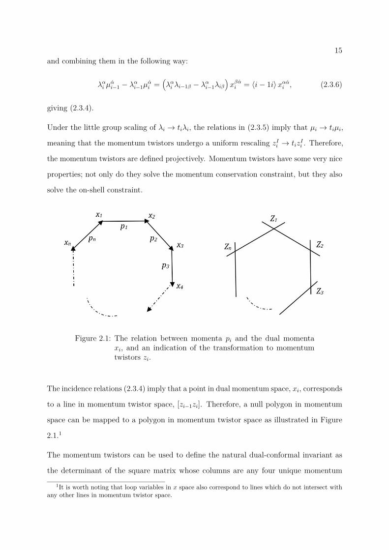
2.1 The relation between momenta pi and the dual momenta xi, and an indic-

ation of the transformation to momentum twistors zi. . . . . . . . 15

3.1 Figures illustrating polygons in P 2 represented as a disc where opposite

points of the disc are identified. In Figure a) we illustrate the fact that

there are four triangles I, II, III, IV all of which have the same three vertices

Z1, Z2, Z3 and all having the same canonical form 〈123〉2/(〈Y 12〉〈Y 23〉〈Y 31〉).

In Figure b) we see a region (shaded area) which has the same canon-

ical form as the quadrilateral [Z1Z2Z3Z4], 〈123〉2/(〈Y 12〉〈Y 23〉〈Y 31〉) +

〈134〉2/(〈Y 13〉〈Y 34〉〈Y 41〉) but which does not represent a good geomet-

rical region as it has spurious boundaries. . . . . . . . . . . . . 32

3.2 Two possibilities for triangulating a polygon. BCFW gives a generalisation

of the left hand side, whereas WLDs give a generalisation of the right hand

side. (for NMHV). . . . . . . . . . . . . . . . . . . . . 34

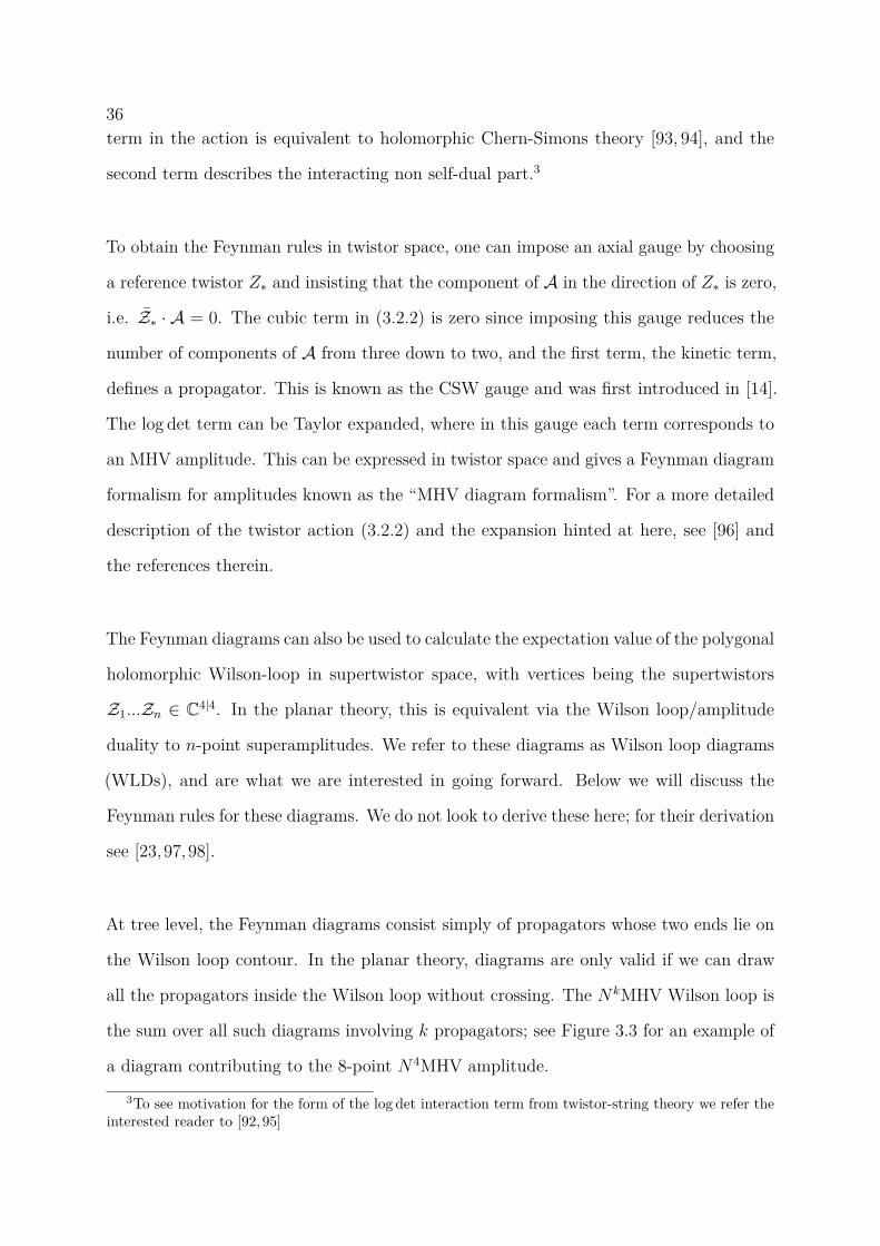
3.3 Example of a Wilson loop diagram which contributes to the 8-point N4MHV

amplitude. . . . . . . . . . . . . . . . . . . . . . . . 37

3.4 Examples of Feynman diagrams in twistor space that contribute to the

6-point NMHV / N2MHV amplitude with their corresponding expressions

following the rules given. . . . . . . . . . . . . . . . . . . 38

3.5 Spurious poles occur when the propagator end reaches the vertex. It is

cancelled by the adjacent diagram. . . . . . . . . . . . . . . 42

xvi3.6 A special case of the spurious pole cancellation that occurs when the

propagator ends are on next-to-adjacent edges, and one propagator end

moves to the vertex closest to the other end. . . . . . . . . . . . 43

3.7 Three diagrams each having a new type of spurious pole occurring when

the propagator ends touch. In the sum of the three diagrams, however, this

pole cancels. Note that although this is drawn at six points for illustrative

purposes, the cancellation only depends on the three sides taking part and

can be directly repeated at n points. . . . . . . . . . . . . . 48

3.8 Three diagrams which when summed cancel the spurious poles illustrated

by the arrows on each diagram. This is a special case of the three way

cancellation. . . . . . . . . . . . . . . . . . . . . . . . 51

3.9 The two possibilities for three way boundary matching. We plot the range

of α on a circle from [−∞,∞] passing through 0 and 1. Black is the range

of α in diagram D1, in red that of α(β) in D2 and in blue the range of

α(γ) in D3. We see there is always a local pairwise matching of the three

diagrams in both cases. In Case 1 D2 and D3 each only overlap with D1

and not with each other. For Case 2 all diagrams overlap the other two. . 54

6.1 Regions I and II clearly have a spurious boundary along the edge [Z1Z3]

despite their canonical forms summing to cancel the associated spurious

pole. . . . . . . . . . . . . . . . . . . . . . . . . . . 146

A.1 The WLDs corresponding to the special three way cancellation, with the

limits of the residues illustrated by the arrows on each WLD. . . . . . 151

D.1 Tree diagrams corresponding to the diagrams given in (4.4.8). The label i

corresponds to the propagator Tqi and the branches of the trees correspond

to the propagators. . . . . . . . . . . . . . . . . . . . . 161

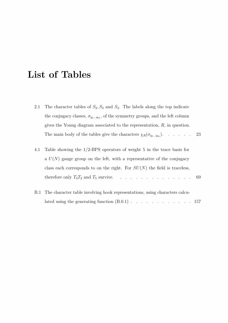
List of Tables

2.1 The character tables of S2, S3 and S4. The labels along the top indicate

the conjugacy classes, σq1...qm , of the symmetry groups, and the left column

gives the Young diagram associated to the representation, R, in question.

The main body of the tables give the characters χR(σq1...qm). . . . . . 23

4.1 Table showing the 1/2-BPS operators of weight 5 in the trace basis for

a U(N) gauge group on the left, with a representative of the conjugacy

class each corresponds to on the right. For SU(N) the field is traceless,

therefore only T3T2 and T5 survive. . . . . . . . . . . . . . . 69

B.1 The character table involving hook representations, using characters calcu-

lated using the generating function (B.0.1) . . . . . . . . . . . . 157

Chapter 1

Introduction

1.1 Introduction

Quantum Field Theory (QFT) is a very important part of the tool kit for any theoretical

physicist due to its broad ranging applications that extend from condensed matter physics

to particle physics and beyond. One of the biggest revolutions in theoretical physics in

the last few decades is the AdS/CFT correspondence, a conjectural relation between

string theory on a d+ 1 dimensional Anti-de-Sitter space and a conformal quantum field

theory living on the d dimensional boundary [1–3]. The discovery of this correspondence

intimately connected two of the most important unsolved problems in theoretical physics;

how to understand non-perturbative gauge theory, and how to quantise gravity. The

most remarkable aspect of the conjecture, and also the property that makes it extremely

difficult to prove, is the strong-weak nature of the duality. The strongly coupled gauge

theory is dual to the weakly interacting stringy physics and vice versa. Therefore, the

strongly coupled regimes of both theories, which otherwise would have been very difficult

to probe, can be studied by investigating the weakly coupled regime of the dual theory and

then using the dictionary provided by the correspondence to move back to the theory of

interest. For a thorough review of AdS/CFT and its many applications see for example [4].

Perhaps the most successful and most studied example of the correspondence is in d = 4

2dimensions, where the maximally supersymmetric CFT known as N = 4 super Yang-Mills

is conjectured to be dual to type IIB string theory on AdS5 × S5.

In order to define the Yang-Mills theory we require two parameters: the coupling gYM and

the rank N of the gauge group (where this thesis will include both U(N) and SU(N)). It

was shown by ’t Hooft [5] that in the limit where the number of colours, N , of the gauge

group becomes large and the ’t Hooft coupling λ = g2YMN is kept finite, a huge amount

of simplifications occur. This limit where N →∞ is known as the “planar” limit.

The simplified nature of N = 4 SYM allows for interesting and unexpected physical and

mathematical structures to be uncovered, and it is often regarded as a toy model to more

realistic theories. Therefore, the study of links between N = 4 SYM and its gravity dual

remains at the forefront of current research today. It is hoped that this will lead to enough

of an understanding of four-dimensional quantum field theories in general that properties

of more realistic theories, that otherwise would have been far more difficult or impossible

to explore, will be uncovered. This thesis will restrict to explorations of different aspects

of N = 4 SYM, particularly in the planar limit, though we will indicate how one or two

of our results are consistent with the relevant results on the gravity side in Chapter 4.

A particularly important set of mathematical objects in any field theory is the set of scat-

tering amplitudes. They are interpreted as the “probabilities” for a particular interaction

to occur and are a key ingredient in the cross sections used by particle colliders. The

ability to compute scattering amplitudes using Feynman rules derived from a Lagrangian

was one of the earliest successes of quantum field theory. However, the calculations very

quickly became intractable as the number of diagrams to compute increased very rapidly

with the number of particles involved in the interaction. Moreover, many cancellations

of the individual terms led to huge simplifications of the final result. The example often

quoted that never ceases to be extremely impressive is the reduction of the 2-to-4 gluon

amplitude result from six pages [6] to a single line [7]! Furthermore, this result only

required slight modifications to give the 2-to-n gluon amplitude; unthinkable from the

Feynman diagram point of view. The remarkable simplicity of the final expression heavily

3indicated that whilst correct, the Feynman diagram approach was not an efficient method

for calculating scattering amplitudes, and led to an explosion of progress in understanding

scattering amplitudes on a more fundamental level.

Many techniques, broadly referred to as “on-shell methods”, were then discovered that

could be used to calculate scattering amplitudes without having to deal with the presence

of the massive gauge redundancies present in the Feynman diagrams. The concept

of “generalised unitarity” [8–10] was developed, which allowed for the evaluation of loop

integrals that were previously inaccessible (see for example [11] and the references therein).

New recursion relations were developed, including BCFW [12,13] and CSW [14] recursions,

which enabled the computation of amplitudes of four points and more starting from three-

point amplitudes, which were fixed purely by Poincaré invariance.

As amplitudes were becoming more well understood, unanticipated symmetries were found

including dual superconformal symmetry [15–18]. The massive amount of symmetry led

to the discovery of a remarkable duality between scattering amplitudes and Wilson

loops [19–24]. In fact, this duality turned out to be a triality between Wilson loops,

scattering amplitudes and correlation functions [25,25–28]. It was then understood that

the dual superconformal symmetry paired with the standard superconformal symmetry

of N = 4 SYM to form a full “Yangian” symmetry [29]. The duality between amplitudes

and correlators has led to some astounding results. For example, the duality was used

along with techniques in graph theory to calculate the 4-point amplitude to an impressive

ten loops [30]. Furthermore, it is projected that any scattering amplitude for any n with

any helicity structure at any loop order may be extractable from the four-point correlator.

This was successfully tested up to seven points and two loops [31].

For the purposes of this thesis, however, we will take advantage of a different aspect of

the triality: the duality between amplitudes and Wilson loops. The duality was first

conjectured by Alday and Maldacena at strong coupling [19], and was later understood in

a very geometrical way via a “fermionic T-duality” [32,33]. This maps a gluon scattering

process to the expectation value of a polygonal Wilson loop with cusps and light-like

4edges determined by the gluon momenta (see [34] for a review). The duality was also

observed at weak coupling by Drummond, Korchemsky and Sokatchev [20], for a specific

set of helicity configurations known as MHV amplitudes. On space-time, the conjecture

has been checked for a number of examples. It was shown using anomalous conformal

Ward identities conjectured in [35] and proven in [36] that the finite part of the 4− and

5−point Wilson loop can be fixed (up to an additive constant), and the functional form

is in agreement with the BDS conjecture [37] for the finite part of the n-point MHV

amplitude when n = 4, 5. The Wilson loop/MHV amplitude duality has also been tested

for arbitrary n at one loop in [21], and up to two loops at n = 6 [38–40].

Reformulating the Wilson loop in twistor space led to the conjecture that the full super-

amplitude (with arbitrary external helicities) is related to a supersymmetric, holomorphic

version of the Wilson loop in twistor space [23]. The conjecture has been proven at

the level of the loop integrand [22, 41]; this thesis shall exploit this duality and remain

restricted to the level of the integrand.

One of the most remarkable discoveries in recent years was the underlying Grassmannian

structure of planar N = 4 [42–46], which resulted in a fundamental reformulation of

our understanding of scattering amplitudes. Previously, locality and unitarity were con-

sidered guiding principles, but understanding the Grassmannian structure moved these

to emergent properties of the overarching principle of positivity. These considerations led

to the discovery of the “Amplituhedron” [47, 48], a geometric object whose boundaries

were determined by the requirement of positivity. Scattering amplitudes are related to

the Amplituhedron by calculating differential forms on the boundary of the object. This

geometric picture has been used to obtain a large amount of all-loop data at the level of

the integrand [49,50]. Whilst we too will be focussing on the integrand in this thesis, it

is worth noting that recently connections to the symbol alphabets, which are properties

of the final (integrated) amplitudes, have been made [51–54]. Furthermore, whilst we will

be focussing on (planar) N = 4, positivity has allowed the discovery of hidden structures

in several other contexts, including the associahedron in bi-adjoint scalar field theory,

5conformal field theory, effective field theory and φ4 theory.

In this thesis we will not only be concerned with amplitudes, but other objects of N = 4

SYM known as operators and correlators. In general, the matching between the two sides

of the AdS/CFT duality is dependent on two things [2, 3]:

1. The energy of an AdS state must match the scaling dimension of a CFT local

operator (we can use CFT local operators rather than states due to the operator-

state correspondence).

2. The correlators of the AdS states and CFT local operators must agree.

In general, the correlators are very hard to calculate explicitly, however in the planar

limit things once again become more straightforward. Here, only the leading term in

the ’t Hooft expansion survives, meaning only planar Feynman diagrams contribute. In

fact, concrete results to all orders in λ can be calculated using powerful mathematical

techniques due to the integrable nature of SYM in this limit [55]. A review of integrability

as it relates to the AdS/CFT correspondence can be found in [56].

It is much more difficult to study the correspondence when allowing for sub-leading terms

in the 1/N expansion or at finite N . However, restricting to a special class of operators

known as the 12 -BPS operators, that are annihilated by half of the sixteen Poincaré

supercharges in the theory, allows for more concrete results to be found even at finite N .

It is of utmost importance to be careful when considering which operator in the CFT is

dual to which state on the string side. Chapter 4 of this thesis shall investigate this issue

for the particular example of the single particle.

Having outlined some of the extensive structure that planar N = 4 SYM exhibits, the

context has been set for the work about to be presented here. We will now outline the

main themes that will be covered in the rest of this thesis.

1.1.1 Outline of the Thesis

The thesis shall be structured as follows:

6- In Chapter 2, we shall present a very brief introduction to some of the technical machinery

that may be useful for the remainder of the thesis. This will include a very brief venture

into N = 4 super Yang-Mills and various ways of representing the external momenta

involved in scattering processes, as well as an introduction to various properties of the

symmetric group Sn which will come in to play in Chapter 4.

- In Chapter 3, we look to determine if twistor Wilson loop diagrams provide an expli-

cit triangulation of the amplituhedron, or any geometric region for that matter. Via

the Wilson loop - amplitude duality, twistor Wilson loop diagrams (WLDs) split the

amplitude into well defined pieces. The expression associated to each diagram is given

by Feynman rules which we shall state, then we will show that each expression has a

natural interpretation on the same space in which the amplituhedron lives. Each term

has spurious poles which cancel algebraically in the sum over all diagrams to give the

amplitude integrand. Therefore, one would expect that the geometric interpretations of

these terms would leave no spurious boundaries when glued together. If this were true,

the WLDs would give a very explicit tesselation of the amplituhedron. We will show that

the diagrams do in fact give a tesselation at NMHV, but for higher helicity values there

is no way to glue together the regions to end up with no spurious boundaries left over.

The work in this chapter is based off of published work given here: [57].

- In Chapter 4, we look to investigate a set of half-BPS operators which are appropriate

for describing single-particle states of superstring theory on AdS5×S5. We refer to these

as single particle operators, and they are defined to be the operators that have vanishing

two-point functions with all multi-trace operators. We find explicit formulae for these

operators and their two point normalisation, then look to give a number of explicit results

for their free theory correlators; this will include all maximally and next-to-maximally

extremal free correlators. We shall also show that at large N the single-particle operator

naturally interpolates between the single-trace operator and the sphere giant graviton.

7The work in this chapter is based off of published work given here: [58].

- In Chapter 5, we give a short description of N2MHV Yangian invariants for N = 4 SYM.

Tree-level amplitudes can be written as a linear combination of Yangian invariants, which

is one of many uses of them. The invariants are very important objects, and a complete

understanding of their properties would be useful. As a small first step, we present all

N2MHV Yangian invaraints mapped to amplituhedron coordinates, where it is hoped it

will be easier to examine their structure more carefully.

- Finally, in Chapter 6 we summarise the main results of the thesis and describe future

work that would be interesting to explore.

We will provide a brief, though slightly more tailored, introduction at the beginning of

Chapters 3, 4 and 5 on the themes relevant specifically to that Chapter, as well as any

more background knowledge that may be useful.

Chapter 2

Review of Concepts

2.1 The N = 4 Supersymmetric Yang-Mills

Lagrangian and Field Content

N = 4 supersymmetric Yang-Mills theory in four dimensions is a very special theory;

the β-function vanishes, therefore the conformal invariance is preserved in the quantum

regime. The symmetry groups of the theory include the conformal group SO(2, 4) which

is then uplifted to the super-conformal group PSU(2, 2|4), as well as a global R-symmetry

SU(4)R ∼ SO(6)R that rotates the charges.

The field content of N = 4 super Yang-Mills consists of six real scalars φi, four fermions

λI and a gauge field Aµ. The scalars transform in the fundamental representation of of

the SO(6) R-symmetry group, while the fermions transform in the fundamental of the

SU(4). All of the fields are forced to transform in the adjoint representation of the gauge

group by the extended supersymmetry; in Chapter 4 we shall consider both U(N) and

SU(N) gauge groups.

Though we do not look to explore this in too much detail, we state the N = 4 SYM

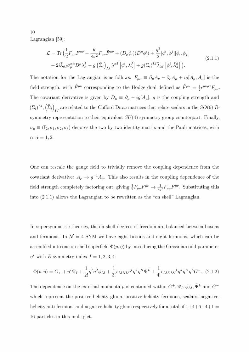
10Lagrangian [59]:

L = Tr(1

2FµνFµν + θ

8π2FµνFµν + (Dµφi)(Dµφi) + g2

2 [φi, φj][φi, φj]

+ 2iλαIσααµ DµλIα − g(Σi

)IJλαI

[φi, λJα

]+ g(Σi)IJ λαI

[φi, λαJ

] ).

(2.1.1)

The notation for the Lagrangian is as follows: Fµν ≡ ∂µAν − ∂νAµ + ig[Aµ, Aν ] is the

field strength, with F µν corresponding to the Hodge dual defined as F µν = 12εµνρσFµν .

The covariant derivative is given by Dµ ≡ ∂µ − ig[Aµ], g is the coupling strength and

(Σi)IJ ,(Σi

)IJ

are related to the Clifford Dirac matrices that relate scalars in the SO(6) R-

symmetry representation to their equivalent SU(4) symmetry group counterpart. Finally,

σµ ≡ (I2, σ1, σ2, σ3) denotes the two by two identity matrix and the Pauli matrices, with

α, α = 1, 2.

One can rescale the gauge field to trivially remove the coupling dependence from the

covariant derivative: Aµ → g−1Aµ. This also results in the coupling dependence of the

field strength completely factoring out, giving 12FµνF

µν → 12g2FµνF

µν . Substituting this

into (2.1.1) allows the Lagrangian to be rewritten as the “on shell” Lagrangian.

In supersymmetric theories, the on-shell degrees of freedom are balanced between bosons

and fermions. In N = 4 SYM we have eight bosons and eight fermions, which can be

assembled into one on-shell superfield Φ(p, η) by introducing the Grassman odd parameter

ηI with R-symmetry index I = 1, 2, 3, 4:

Φ(p, η) = G+ + ηIΨI + 12!η

IηJφIJ + 13!εIJKLη

IηJηKΨL + 14!εIJKLη

IηJηKηLG−. (2.1.2)

The dependence on the external momenta p is contained within G+,ΨI , φIJ , ΨL and G−

which represent the positive-helicity gluon, positive-helicity fermions, scalars, negative-

helicity anti-fermions and negative-helicity gluon respectively for a total of 1+4+6+4+1 =

16 particles in this multiplet.

112.2 Scattering Amplitudes in Planar N = 4 SYM

Scattering amplitudes in planar SYM exhibit many beautiful mathematical properties,

some of which were named briefly in the introduction. Generally an amplitude will involve

some integration, which is often very non-trivial. For the considerations of this thesis,

however, we shall restrict ourselves to the integrand only, i.e. before the integration is

performed. The triality mentioned in the introduction holds at the level of the integrand,

which will be particularly important for Chapter 3 of this thesis. The part of the integrand

of the amplitude that is not dependent on the helicity of the particles involved are functions

dependent on the momenta, pa.

An n-point (planar) super-amplitude can be expanded over the Grassmann variables ηIawith particle number a = 1, . . . , n, giving

A = An;2 +An;3 + . . .+An;n−2, (2.2.1)

where each term An;k is a homogeneous polynomial in ηI of degree 4k, with (ηa)4 ≡ ηIa.

Before going any further, it is useful to introduce the spinor-helicity formalism, where we

write the external kinematic data as

pµa(σµ)αα =

p0a − p3

a −p1a + ip2

a

−p1a − ip2

a p0a + p3

a

≡ pααa ≡ λαa λαa (2.2.2)

where εαβ = −εαβ are the anti-symmetric epsilon tensors with α ∈ 1, 2, α ∈ 1, 2.

Let A(l)n;k represent the l-loop n-particle NkMHV super-amplitude. The supersymmetric

generalisation of the Parke-Taylor formula is given by [60]:

A(0)n;2 =

δ4(∑n

a=1 λαa λ

αa

)δ8(∑n

i=1 λαaη

Ia

)〈12〉 . . . 〈n1〉 , (2.2.3)

where 〈ab〉 ≡ εαβλαaλ

βb and the second delta function is a Grassmann delta function that

ensures conservation of supermomentum.

It is often convention that the super-amplitude is divided through by the MHV tree-level

super-amplitude A(0)n;2 given by (2.2.3), which roughly speaking subtracts eight powers of

12η off of each partial amplitude leading to

A = An;0 + An;1 + . . .+ An;n−4, (2.2.4)

with the standard normalisation An;0 = 1. Once again, the A are all homogeneous

polynomials in ηI of degree 4k. Each term in this sum is then further expanded over loop

variables

An;k =∞∑l=0

alA(l)n;k, (2.2.5)

where we have now dropped the ’hat’ notation for A with the understanding that when

amplitudes are referred to in this thesis they will be divided by the tree level MHV

super-amplitude. We refer to the expression A(l)n;k as the l-loop integrand of the amplitude.

It can written as some combination of rational functions dependent on the momenta

multiplied by Yangian invaraints:

A(l)n;k =

∑ij

cijRk;i(ηa, p1, . . . pn)× I(l)j (p1, . . . , pn+l). (2.2.6)

Notice that the rational functions I are dependent on the external momenta and all loop

momenta for a fixed l. Furthermore, the η dependence lies within the k degree Yangian

invaraints R, meaning they act as generating functions for different helicity configurations

of the superparticle given by (2.1.2).

When studying amplitudes in N = 4 SYM, one often focusses on the gluon amplitude.

The n-particle NkMHV gluon amplitude refers to the interaction between (k+2) negative

helicity gluons and (n− k − 2) positive helicity gluons. The simplest case corresponds to

the k = 0 case, known as the MHV gluon amplitude (see (2.2.3)). The highest value of k

that results in a non-trivial gluon amplitude is known as the anti-MHV amplitude, or the

Nn−4MHV = MHV amplitude. The amplitudes involving all positive helicity gluons, or

all bar one positive with one being negative, vanish by the supersymmetric ward identities;

as do their parity conjugates [61, 62]. Whilst it may seem odd at first glance that only

gluon amplitudes have been considered, they can in fact be used to get the full super-

amplitude using the superparticle expansion given by (2.1.2). The supersymmetric Ward

13identities relate all particle amplitudes that have the same order of η dependence [62]. For

example, at η8 (before dividing by the tree-level MHV amplitude), the n-particle MHV

gluon amplitude involving two negative gluons (∼ η4η4) with the rest positive gluons

(∼ η0) is related to an MHV amplitude with four scalars (∼ η2η2η2η2) and (n−4) positive

gluons.

Finally, since most of this thesis will be concerned with N = 4 SYM in the planar limit,

it is worth noting one final simplification. In the planar limit, one can fix an ordering

of the external momenta and calculate the “colour-ordered amplitude” corresponding to

this ordering, then find the full tree level super-amplitude by summing over all non-cyclic

permutations of the external momenta:

Atreen = gn−2 ∑

σ∈Sn/Zn

Tr(T aσ(1) . . . T aσ(n)

)Atreen

(p

Λσ(1)σ(1) . . . p

Λσ(n)σ(n)

). (2.2.7)

Here, Λa = ±1 gives the helicity of particle a, g is the coupling. Therefore, it makes sense

to choose the canonical ordering 1, . . . , n. For more information on this, or any topic

introduced in this section, the interested reader should refer to for example [61, 62] and

the references therein.

2.3 Super Momentum Twistors and Bosonisation to

Amplituhedron Coordinates

In this section we introduce the so-called “momentum twistors” [63,64], provide conven-

tions and review some of their basic properties. We then uplift to include supersymmetry,

and show how to bosonise these super-momentum twistors to write them in “amplituhed-

ron coordinates” [47,63].

142.3.1 Momentum Twistors and Supermomentum Twistors

Momentum twistors are defined in terms of dual coordinates xi, defined by

λαi λαi ≡ pααi ≡ xααi+1 − xααi , (2.3.1)

where λi and λi are the usual spinor-helicity variables and pααi are four dimensional null

momenta. Multiplying (2.3.1) by λiα gives zero on the left hand side, leading to the

following (bosonic) incidence relations:

xααi λiα = xααi+1λiα ≡ µαi , (2.3.2)

where i = 1, ..., n labels the particle number and α ∈ 1, 2, α ∈ 1, 2. Momentum

conservation in dual momentum coordinates is manifest. This can be visualised as a

null polygon with the xi as the vertices, constructed by arranging the external (null)

momenta head-to-tail (see Figure 2.1). There is a conformal symmetry that acts on the

dual momenta known as the dual conformal group, which was shown to be a symmetry

of planar N = 4 SYM [15–17] and ABJM theory [65–67].

Bosonic momentum twistors are then defined by taking each pair λαi and µαi and organising

them as four-component projective vectors, zAi :

zAi ≡(λαi , µ

αi

)∈ C4, (2.3.3)

where A ∈ 1, ..., 4 are indices in the fundamental representation of the dual conformal

group, SU(4). Using the incidence relation and (2.3.1) one finds that the x coordinates

satisfy the incidence relations

xααa = λαi µαi−1 − λαi−1µ

αi

〈i− 1i〉 , (2.3.4)

where 〈i− 1i〉 ≡ εαβλαi−1λ

βi . These incidence relations can be derived by identifying two

adjacent momentum-twistor points with a single space-time coordinate,

xααi λiα = µαi , xααi λi−1α = µαi−1, (2.3.5)

15and combining them in the following way:

λαi µαi−1 − λαi−1µ

αi =

(λαi λi−1β − λαi−1λiβ

)xβαi = 〈i− 1i〉xααi , (2.3.6)

giving (2.3.4).

Under the little group scaling of λi → tiλi, the relations in (2.3.5) imply that µi → tiµi,

meaning that the momentum twistors undergo a uniform rescaling zIi → tizIi . Therefore,

the momentum twistors are defined projectively. Momentum twistors have some very nice

properties; not only do they solve the momentum conservation constraint, but they also

solve the on-shell constraint.

Figure 2.1: The relation between momenta pi and the dual momentaxi, and an indication of the transformation to momentumtwistors zi.

The incidence relations (2.3.4) imply that a point in dual momentum space, xi, corresponds

to a line in momentum twistor space, [zi−1zi]. Therefore, a null polygon in momentum

space can be mapped to a polygon in momentum twistor space as illustrated in Figure

2.1.1

The momentum twistors can be used to define the natural dual-conformal invariant as

the determinant of the square matrix whose columns are any four unique momentum

1It is worth noting that loop variables in x space also correspond to lines which do not intersect withany other lines in momentum twistor space.

16twistors:

〈ijkl〉 ≡ det [zizjzkzl] = εABCDzAi z

Bj z

Ck z

Dl . (2.3.7)

The expression generalises to higher point brackets upon adding supersymmetry then

bosonising; this will be discussed below. These invariants are related to the dual space via

x2i,j = (xi − xj)2 → 〈i− 1ij − 1j〉. Furthermore, this four bracket can be used to express

the linear dependence of any five momentum twistors as a generalised Schouten identity

zi 〈jklm〉+ (cyclic in i, j, k, l,m) = 0. (2.3.8)

In order to extend these momentum twistors to supersymmetric theories, in analogy to

(2.3.1), we define dual super momenta as

qαIi ≡ λαi ηIi ≡ θαIi+1 − θαIi , (2.3.9)

with θn+1 = θ1. The momentum twistors can now be uplifted to super-momentum

twistors,

ZAi ≡(λαi , µ

αi ; θIi · λi

)≡(zAi ;χIi

)∈ C4|4, (2.3.10)

where A = 1, ..., 4 and I = 1, ..., 4 are four component bosonic and fermionic indices

respectively, which we combine to form the eight component index denoted by A = 1, ..., 8.

The coordinates χIi are Grassman-odd, and hold the necessary properties for defining the

superconformal invariant that will be discussed below. Now we have incidence relations

for the bosonic coordinates given in (2.3.2) and an additional set of relations for the

fermionic components of the super-momentum twistors:

θαIi λiα = θαIi+1λiα ≡ χIi . (2.3.11)

Furthermore, by equating the same superspace point to two super-momentum twistors

χIi = θαIi λiα and χIi−1 = θαIi λi−1α, in a similar way to (2.3.6), we end up with a fermionic

equivalent of (2.3.4):

θIiα = λiαχIi−1 − λi−1αχ

Ii

〈i− 1i〉 . (2.3.12)

17Beyond the MHV sector, superamplitudes can be written in terms of dual superconformal

invariants [16]. At NMHV, the dual superconformal invariants are known as R invariants

[64], and are defined as follows

[ijklm] ≡δ0|4

(χIi 〈jklm〉+ · · ·+ χIm 〈ijkl〉

)〈jklm〉 〈klmi〉 〈lmij〉 〈mijk〉 〈ijkl〉

, (2.3.13)

where the delta function in the numerator is a fermionic delta function. The BCFW

representation of the tree level n-point NMHV amplitude can be written in momentum

twistor space as

MNMHVn = 1

2∑i,j

[1ii+ 1jj + 1] . (2.3.14)

The CSW representation of the same amplitude [43, 68] is obtained by replacing the

seemingly special point “1” in this formula with a general momentum twistor, Z1 → Z∗.

A toy example of these two representations is illustrated in Figure 3.2 and is discussed

in the surrounding text. Furthermore, the general supermomentum twistor Z∗ will be

discussed more in Chapter 3 when Wilson loops are introduced.

2.3.2 Bosonisation of Supermomentum Twistors

It will be useful to switch to “bosonised superspace”, where we will refer to the bosonised

supermomentum twistors as being written in “amplituhedron coordinates”. We provide a

brief description of this process here following [47,63].

To begin, we introduce a particle-independent fermionic variable φpI , where p = 1, ..., k

and I = 1, ..., 4 is an R-symmetry index. The φ variables are then contracted with the

Grassmann odd χ variables of the supermomentum twistors to give Grassmann even

variables ξpi = χIiφpI . The range of the p index is dependent on the helicity structure

of the superamplitude. For NkMHV amplitudes, p = 1, ..., k, therefore bosonising this

superspace maps from the dimension (4|4) momentum supertwistors to purely bosonic

18vectors in 4 + k dimensions:

C4|4 → C4+k

Z (z, χ)→ Z (z, ξ = χ · φ) .(2.3.15)

It is worth noting that the amplituhedron space itself is a subset of Gr(k, 4+k), hence why

we often refer to these bosonised supermomentum twistors as being in “amplituhedron

coordinates”. Using this map allows for non-trivial superconformal identities to become

manifest in generalised Schouten identities (see (2.3.8)). Bosonising the momentum

twistors is an essential step before being able to associate a geometry to the Wilson loop

diagrams that we will introduce in Chapter 3.

We look to see how bosonising the NMHV amplitude (2.3.14) allows us to write it in

a very simple way, which can be related to the volume of a polytope. Rewriting the

R-invariant [ijklm] by introducing a fermionic four indexed variable φI ,

∫d4φφ4 δ

0|4(χIi 〈jklm〉+ · · ·+ χIm 〈ijkl〉

)〈jklm〉 〈klmi〉 〈lmij〉 〈mijk〉 〈ijkl〉

(2.3.16)

where φ4 = ∏I φI . A fermionic delta function satisfies the identity δ0|4(θ) = θ4, therefore

the numerator of (2.3.16) becomes

φ4δ0|4(χIi 〈jklm〉+ · · ·+ χIm 〈ijkl〉

)= φ4

(χI4i 〈jklm〉

4 + · · ·+ χI4m 〈ijkl〉4)

= φ1φ2φ3φ4χ1iχ

2iχ

3iχ

4i 〈jklm〉

4 + · · ·+ φ1φ2φ3φ4χ1mχ

2mχ

3mχ

4m 〈ijkl〉

4

= (φ · χi 〈jklm〉 − φ · χj 〈iklm〉+ ...)4 . (2.3.17)

For NMHV amplitudes k = 1, so bosonising the supermomentum twistors gives

ZAi ≡(zAi ;χIiφI

)∈ C5, (2.3.18)

where A = 1, ..., 5 labels the bosonic singlet that the supermomentum twistor has now

been mapped to. With this we define the five bracket

〈ijklm〉 ≡ det [ZiZjZkZlZm] . (2.3.19)

19Expanding this determinant along the bottom row gives precisely (2.3.17), therefore the

R-invariant can be written as the dual conformal ratio

[ijklm] = 〈ijklm〉4

〈ijkl〉 〈jklm〉 〈klmi〉 〈lmij〉 〈mijk〉. (2.3.20)

The bosonised coordinates can be generalised to arbitrary helicity by the map (2.3.15),

and the following (4 + k)-bracket can be defined:

〈i1i2...ik+4〉 ≡ det[Zi1Zi2 ...Zik+4

]. (2.3.21)

As a further example of how these coordinates can be useful, the MHV n-point tree level

superamplitude has the following very simple form in amplituhedron coordinates:

A(0)n;n−4 = 〈12...n〉4

〈1234〉 〈2345〉 ... 〈n123〉 . (2.3.22)

2.4 Mathematical Preliminaries: Permutations and

Partitions

In this section, we look to introduce some mathematical tools that will be very useful in

particular for Chapter 4. The use of permutations has been a significant technical step

in allowing the explicit construction of operator bases and the calculation of correlators.

Here we look to give a brief overview of some of the tools that we will make use of in

Chapter 4 when constructing our own bases of 1/2-BPS operators.

2.4.1 The Symmetric Group

The symmetric group, Sn, is the group of permutations of n objects. The elements of this

group are often written in cycle notation, for example (123) is the reshuffling of the labels

1→ 2, 2→ 3, 3→ 1. The Young diagrams with n boxes provide a nice way of labelling

the representations of the symmetric group Sn. If λi denotes the length of row i, the set

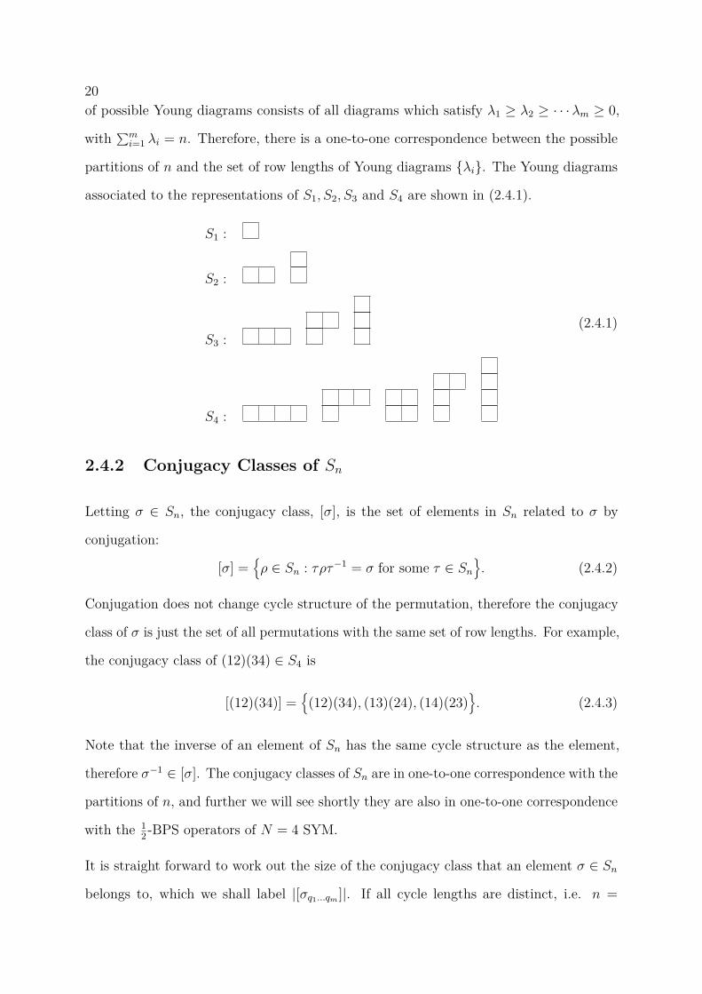
20of possible Young diagrams consists of all diagrams which satisfy λ1 ≥ λ2 ≥ · · ·λm ≥ 0,

with ∑mi=1 λi = n. Therefore, there is a one-to-one correspondence between the possible

partitions of n and the set of row lengths of Young diagrams λi. The Young diagrams

associated to the representations of S1, S2, S3 and S4 are shown in (2.4.1).

S1 :

S2 :

S3 :

S4 :

(2.4.1)

2.4.2 Conjugacy Classes of Sn

Letting σ ∈ Sn, the conjugacy class, [σ], is the set of elements in Sn related to σ by

conjugation:

[σ] =ρ ∈ Sn : τρτ−1 = σ for some τ ∈ Sn

. (2.4.2)

Conjugation does not change cycle structure of the permutation, therefore the conjugacy

class of σ is just the set of all permutations with the same set of row lengths. For example,

the conjugacy class of (12)(34) ∈ S4 is

[(12)(34)] =

(12)(34), (13)(24), (14)(23). (2.4.3)

Note that the inverse of an element of Sn has the same cycle structure as the element,

therefore σ−1 ∈ [σ]. The conjugacy classes of Sn are in one-to-one correspondence with the

partitions of n, and further we will see shortly they are also in one-to-one correspondence

with the 12 -BPS operators of N = 4 SYM.

It is straight forward to work out the size of the conjugacy class that an element σ ∈ Sn

belongs to, which we shall label |[σq1...qm ]|. If all cycle lengths are distinct, i.e. n =

21q1 + . . . + qm with qi 6= qj, the size of the conjugacy classes are simply n!∏m

i=1 qi. If there

are multiple cycles of the same length, i.e. some qi = qj in the partition of n, then these

cycles are interchangeable and we have to divide by this symmetry. To deal with this

case, let λ1, λ2, . . . , λr be the distinct cycle lengths of the permutation σ and k1, k2, . . . , kr

by the number of cycles of each of those lengths respectively, such that ∏rj=1 λ

kjj = ∏m

i=1

and ∑rj=1 kjλj = p. Therefore, the number of elements in a conjugacy class labelled by

q1 . . . qm is given by

|[σq1...qm ]| = p!∏ri=1 ki!λkii

. (2.4.4)

Note that the denominator is in fact the size of the symmetry group, Sym(σ), the subgroup

of Sn that preserves σ under conjugation.

2.4.3 Dimension of Sn

As noted above, the Young diagrams constructed using p boxes label the representations

of Sp. For example, the diagram with p boxes in the first row labels the one-dimensional

trivial representation, and the diagram with p boxes in the first column labels the other

one-dimensional irreducible representation, the sign representation.

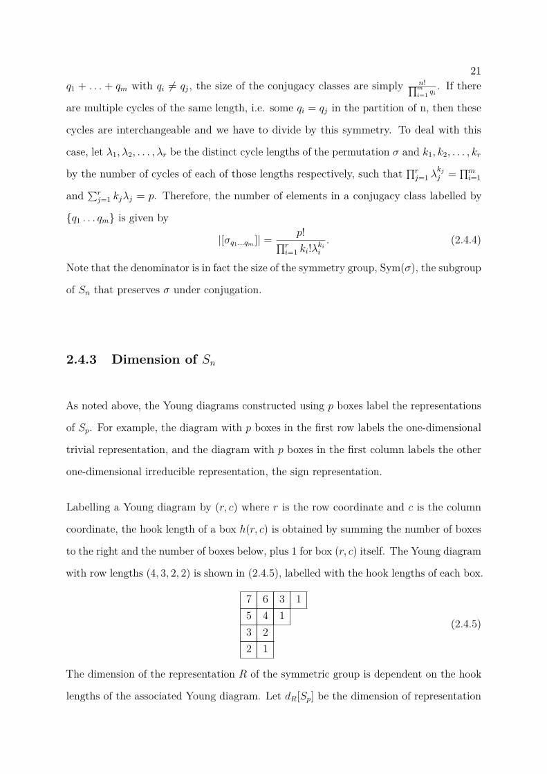
Labelling a Young diagram by (r, c) where r is the row coordinate and c is the column

coordinate, the hook length of a box h(r, c) is obtained by summing the number of boxes

to the right and the number of boxes below, plus 1 for box (r, c) itself. The Young diagram

with row lengths (4, 3, 2, 2) is shown in (2.4.5), labelled with the hook lengths of each box.

7 6 3 15 4 13 22 1

(2.4.5)

The dimension of the representation R of the symmetric group is dependent on the hook

lengths of the associated Young diagram. Let dR[Sp] be the dimension of representation

22R of Sp. The dimension is given by

dR[Sp] = n!∏(r,c)∈R h(r, c) , (2.4.6)

where the product in the denominator is over all hook lengths of the Young diagram. For

example, the dimension of the representation associated to the example in (2.4.5) is given

by

d4,3,2,2(S11) = 11!7 · 6 · 3 · 5 · 4 · 3 · 2 · 2 = 1, 320. (2.4.7)

2.4.4 Characters

Representations can be associated to matrices known as representing matrices. There are

many different ways of constructing these matrices, e.g. for the symmetric group there

are the natural and semi-normal representations constructed in [69] to name only a few.

The character of a representation is the trace of its representation matrix. It is a constant

on conjugacy classes of the group, and as such is known as a class function.

When finding an explicit formula for the single particle operators discussed in the next

section, the characters of interest will be those of the symmetric group. The characters

of S2, S3 and S4 are shown in their character tables in Table 2.1.

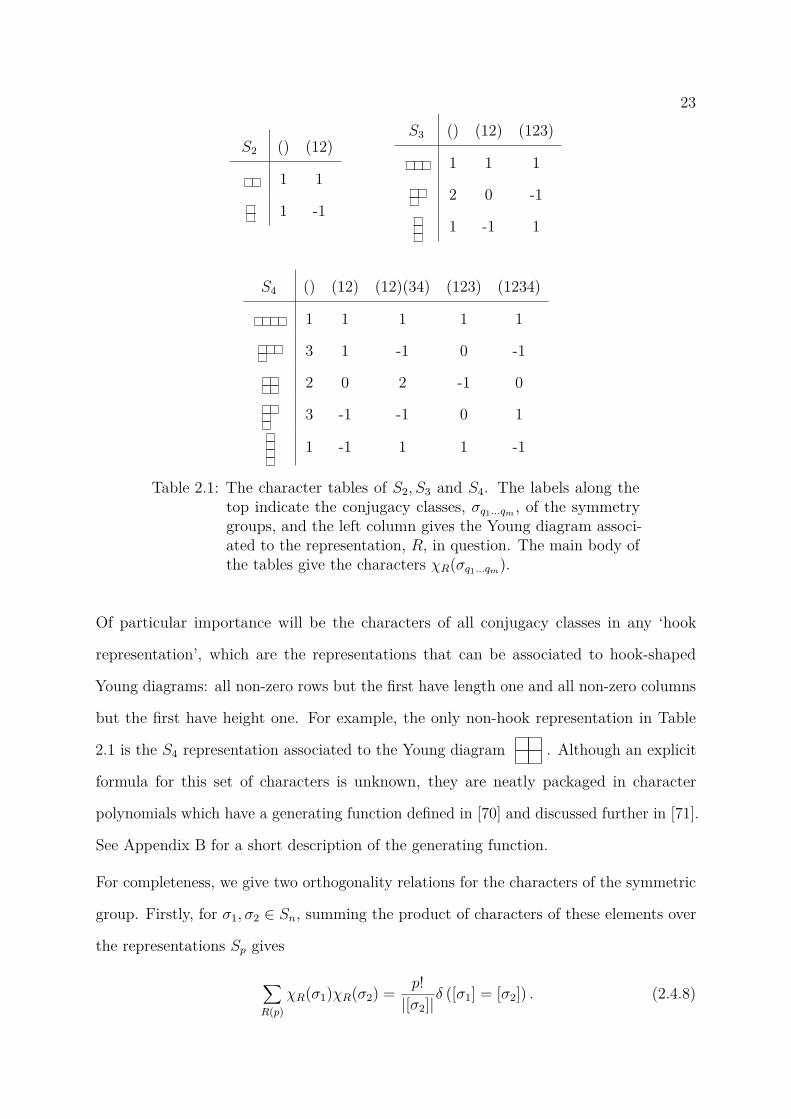
23

S2 () (12)

1 1

1 -1

S3 () (12) (123)

1 1 1

2 0 -1

1 -1 1

S4 () (12) (12)(34) (123) (1234)

1 1 1 1 1

3 1 -1 0 -1

2 0 2 -1 0

3 -1 -1 0 1

1 -1 1 1 -1

Table 2.1: The character tables of S2, S3 and S4. The labels along thetop indicate the conjugacy classes, σq1...qm , of the symmetrygroups, and the left column gives the Young diagram associ-ated to the representation, R, in question. The main body ofthe tables give the characters χR(σq1...qm).

Of particular importance will be the characters of all conjugacy classes in any ‘hook

representation’, which are the representations that can be associated to hook-shaped

Young diagrams: all non-zero rows but the first have length one and all non-zero columns

but the first have height one. For example, the only non-hook representation in Table

2.1 is the S4 representation associated to the Young diagram . Although an explicit

formula for this set of characters is unknown, they are neatly packaged in character

polynomials which have a generating function defined in [70] and discussed further in [71].

See Appendix B for a short description of the generating function.

For completeness, we give two orthogonality relations for the characters of the symmetric

group. Firstly, for σ1, σ2 ∈ Sn, summing the product of characters of these elements over

the representations Sp gives

∑R(p)

χR(σ1)χR(σ2) = p!|[σ2]|δ ([σ1] = [σ2]) . (2.4.8)

24Secondly, for representations R, S of Sp, summing over the elements of Sp gives

∑σ∈Sp

χR(σ)χS(σ) = n!δRS. (2.4.9)

2.4.5 Weights of U(N) Representations

Young diagrams can be associated to U(N) representations as well as Sn representations.

Irreducible representations of GL(N) are labelled by Young diagrams with at most N

rows, but arbitrary number of columns. Representations of the subgroup U(N) ⊂ GL(N)

are the same and are also irreducible. For example, some representations of U(2 are given

by

U(2) : 1 · · · , (2.4.10)

where the first representation is the trivial representation that maps every element of

U(2) to the same complex number. For more details on U(N) representation theory

and its relation to the symmetric group, the interested reader is encouraged to see for

example [72,73].

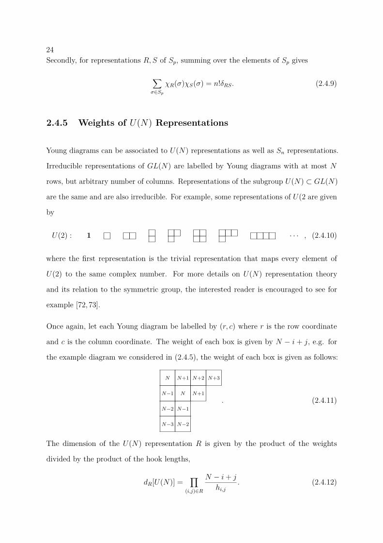
Once again, let each Young diagram be labelled by (r, c) where r is the row coordinate

and c is the column coordinate. The weight of each box is given by N − i + j, e.g. for

the example diagram we considered in (2.4.5), the weight of each box is given as follows:

N N+1 N+2 N+3

N−1 N N+1

N−2 N−1

N−3 N−2

. (2.4.11)

The dimension of the U(N) representation R is given by the product of the weights

divided by the product of the hook lengths,

dR[U(N)] =∏

(i,j)∈R

N − i+ j

hi,j. (2.4.12)

25For the example in (2.4.11), the dimension would be given by

d4,3,2,2(U(N)) = N2(N − 1)2(N + 1)2(N − 2)2(N + 2)(N − 3)(N + 3)7 · 6 · 3 · 5 · 4 · 3 · 2 · 2 . (2.4.13)

Another quantity that will come in useful for later considerations is the product of the

weights by itself. Denoting this quantity fR,

fR ≡∏

(i,j)∈R(N − i+ j) = p!dR (U(N))

dR (Sp). (2.4.14)

2.4.6 Power Set

The final object that will prove useful when writing an explicit formula for the single

particle operators is the power set. The power set is the set of all subsets of a set S,

denoted by P(S), which includes the empty set and the full set S itself. For example, let

S = (3, 2, 1); the power set is given by

P(3, 2, 1) =, 1, 2, 3, 2, 1, 3, 1, 3, 2, 3, 2, 1

. (2.4.15)

Furthermore, let s ∈ P(S). Then |s| denotes the number of elements of the subset s and

Σ(s) denotes the total of all the elements in s, Σsi∈ssi. For example, for s = 3, 2, 1 (a

member of P in (2.4.14)) we have |s| = 3 and Σ(s) = 6.

Chapter 3

The Twistor Wilson Loop and the

Amplituhedron

3.1 Introduction

The amplituhedron provides a beautiful description of perturbative superamplitude in-

tergrands in N = 4 SYM. Inspired by the polytope structure of the six point NMHV

scattering amplitude, first described by Hodges [63] then developed by Arkani-Hamed et

al [74], Arkani-Hamed and Trnka interpreted the integrands of amplitudes in the planar

theory as generalised polyhedra in positive Grassmannians called amplituhedra [47,48]1.

The tree amplituhedron A(m)n,k , with k + m ≤ n, is defined as the image of the positive

Grassmannian Gr+(k, n) of k-planes in n dimensions into Gr(k,m + k). The positivity

here dictates that all maximal (k × k) minors are non-negative. The map is induced

by the n × (k + m) matrix of bosonised external kinematic data, ZAi with i = 1, ..., n

(see section 2.3), where all of the ordered maximal minors must also be positive. The

amplituhedron is given by the set

A(m)n,k (Z) = Y ⊂ Gr(k, k +m) : Y Aα = CαiZ

Ai for C ∈ Gr+(k, n) (3.1.1)

1A second definition of the amplituhedron was elucidated in [75]; a topological definition directly inmomentum-twistor space defined using sign-flip conditions on sequences of twistor invariants.

28with A = 1, ..., k +m and α = 1, ..., k. The case of m = 4 is of most interest to physics,

as it provides a geometric basis for the computation of scattering amplitudes in N = 4

supersymmetric Yang-Mills (SYM). The spaces involving the m = 4 amplituhedron are

mostly what will be considered in the rest of this chapter (aside from the toy model

discussed in the next section which corresponds to m = 2).

Before moving on, it is worth noting that the amplituhedron is a well-defined and in-

teresting mathematical object for any m. The m = 1 amplituhedron can be identified

with the complex of bounded faces of a cyclic hyperplane arrangement [76]. The m = 2

amplituhedron has a very beautiful combinatorial structure and has been well studied over

the last few years [75,77–81]. In fact, despite mostly being thought of as the toy-model

for the m = 4 case, the m = 2 amplithedron has its own applications in physics. The

m = 2, k = 2 amplituhedron governs the geometry of scattering amplitudes in the ‘MHV’

sector of N = 4 SYM, and the m = 2 amplituhedron for general k has connections with

the NMHV sector (and geometries of loop amplitudes) [82].

The scattering amplitude can be related to the canonical form of them = 4 amplituhedron;

a differential form with logarithmic singularities on the boundary and no singularities in

the interior. 2 Therefore, one must consider how to calculate this canonical form. One

way to construct it, which in principal is completely general and straightforward, is by

finding a triangulation of the amplituhedron and summing the canonical forms of all

of the pieces. Triangulating the subspace amounts to finding a non-overlapping set of

(4k)-dimensional cells in Gr+(k, n); there have been a number of recent studies relating

to this, for example [81,83–86].

Although early polytope interpretations involved considering amplitudes via twistor

Wilson loop diagrams (WLDs), the amplituhedron itself instead arose from consider-

ing the BCFW method of obtaining amplitudes. However, the WLDs seem to lend

themselves very naturally and directly to a geometrical interpretation; in this chapter we

wish to look again at the relationship between WLDs and the amplituhedron. Previous

2To see how the definition can be extended to include loops, see [47].

29work examining the connection between them includes [87–89], where in particular the

latter illustrated that the WLDs give a natural description of the physical boundary of the

amplituhedron. Here, we examine whether it is possible to use the WLDs to define a tes-

sellation of the amplituhedron, or further a tessellation of any “good” geometrical region.

We define a good geometrical region as a region that contains no spurious boundaries,

only physical boundaries that correspond to poles of the amplitude.

It should be highlighted here that we make no assumptions about positivity, convexity,

or any particular specific form for the geometrical shape that could correspond to the

WLDs. Our assumptions are only that each WLD can be assocated with a region of

amplituhedron space in such a way that the canonical form of that region gives back the

WLD. As we will see, each WLD contains spurious poles which geometrically correspond

to spurious boundaries. We wish to give an answer to the following question: is it possible

to associate a geometrical region to each WLD such that all spurious boundaries glue

together correctly (locally) pairwise with those of other diagrams so that the union of all

regions leaves no unmatched spurious boundaries.

The chapter will be organised as follows: in section 3.2 we will give a brief description of

Wilson loop diagrams and show how to naturally associate a volume form in Gr(k, k + 4)

(the space in which the amplituhedron lives) to a WLD, in section 3.3 we show that each

WLD can be associated with a tile in the tessellation of the amplituhedron, but in section

3.4 prove that for higher MHV degree this is not possible. More concretely, we prove

that there does not exist a set of tiles whose canonical forms correspond to WLDs that

glue together to form a geometry with no spurious boundaries. Firstly, however, we shall

introduce the toy model which will prove a useful starting point for the considerations of

the rest of this chapter.

This chapter is based off of work completed in [57]. Work completed at the same time

dealing with the same problem using a different approach was discussed by Agarwala and

Marcott in [90].

303.1.1 Toy Model: polygons in P 2

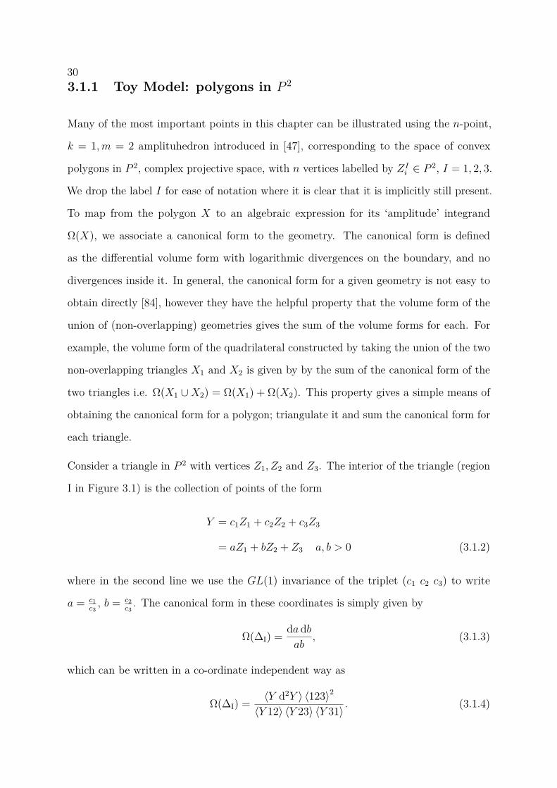
Many of the most important points in this chapter can be illustrated using the n-point,

k = 1,m = 2 amplituhedron introduced in [47], corresponding to the space of convex

polygons in P 2, complex projective space, with n vertices labelled by ZIi ∈ P 2, I = 1, 2, 3.

We drop the label I for ease of notation where it is clear that it is implicitly still present.

To map from the polygon X to an algebraic expression for its ‘amplitude’ integrand

Ω(X), we associate a canonical form to the geometry. The canonical form is defined

as the differential volume form with logarithmic divergences on the boundary, and no

divergences inside it. In general, the canonical form for a given geometry is not easy to

obtain directly [84], however they have the helpful property that the volume form of the

union of (non-overlapping) geometries gives the sum of the volume forms for each. For

example, the volume form of the quadrilateral constructed by taking the union of the two

non-overlapping triangles X1 and X2 is given by by the sum of the canonical form of the

two triangles i.e. Ω(X1 ∪X2) = Ω(X1) + Ω(X2). This property gives a simple means of

obtaining the canonical form for a polygon; triangulate it and sum the canonical form for

each triangle.

Consider a triangle in P 2 with vertices Z1, Z2 and Z3. The interior of the triangle (region

I in Figure 3.1) is the collection of points of the form

Y = c1Z1 + c2Z2 + c3Z3

= aZ1 + bZ2 + Z3 a, b > 0 (3.1.2)

where in the second line we use the GL(1) invariance of the triplet (c1 c2 c3) to write

a = c1c3, b = c2

c3. The canonical form in these coordinates is simply given by

Ω(∆I) = da dbab

, (3.1.3)

which can be written in a co-ordinate independent way as

Ω(∆I) = 〈Y d2Y 〉 〈123〉2

〈Y 12〉 〈Y 23〉 〈Y 31〉 . (3.1.4)

31Here 〈123〉 is the determinant of the matrix made by having Z1, Z2 and Z3 as its columns,

and one can easily get from (3.1.4) to (3.1.3) by plugging in the definition of Y above.

Moving on to the next simplest polygon, the quadrilateral with vertices Z1, Z2, Z3 and Z4

(see the right hand side of Figure 3.1) can be triangulated into two adjacent triangles with

vertices Z1, Z2, Z3 and Z1, Z3, Z4. The triangles have two co-dimension one boundaries

each that are proper boundaries of the quadrilateral, and share a co-dimension one

boundary that is not a boundary of the quadrilateral; the line [Z1Z3]. This is referred to

as “spurious”; the canonical form of each triangle has a log divergence on this boundary,

Y → αZ1 + βZ3. To calculate the canonical form of the quadrilateral we sum the forms

of the two triangles:

Ω(∆4)

= 〈123〉2 〈Y d2Y 〉〈Y 12〉 〈Y 23〉 〈Y 31〉 + 〈134〉2 〈Y d2Y 〉

〈Y 13〉 〈Y 34〉 〈Y 41〉

=

(〈123〉2 〈Y 34〉 〈Y 41〉 − 〈134〉2 〈Y 12〉 〈Y 23〉

)〈Y 12〉 〈Y 23〉 〈Y 34〉 〈Y 41〉 〈Y 31〉

⟨Y d2Y

⟩. (3.1.5)

Adding and subtracting 〈123〉 〈143〉 〈Y 34〉 〈Y 12〉 from the numerator and using the fol-

lowing relations

〈124〉 〈1Y 3〉 = 〈12Y 〉 〈143〉+ 〈1Y 4〉 〈123〉 ,

〈342〉 〈31Y 〉 = 〈341〉 〈32Y 〉+ 〈312〉 〈34Y 〉 ,(3.1.6)

we can re-write (3.1.5) as

Ω(∆4)

= (〈Y 12〉 〈234〉 〈341〉+ 〈Y 34〉 〈123〉 〈412〉)〈Y 12〉 〈Y 23〉 〈Y 34〉 〈Y 41〉

⟨Y d2Y

⟩, (3.1.7)

which is in agreement with the canonical form for the quadrilateral calculated in [84]. We

see in summing the canonical forms of the two triangles that the spurious pole cancels out

and the resulting form indeed only has log divergences on the boundary of the quadrilateral

itself.

A unique canonical form is associated to each polygon, however the reverse is not true;

multiple geometries can have the same canonical form. For example, there are four

inequivalent geometries in P 2 that are associated with the canonical form (3.1.4), given

32

III

II

III

III

IV

IV

Z2Z3

Z1

I

II

II

Z1

Z2Z3

Z4

Figure 3.1: Figures illustrating polygons in P 2 represented as a discwhere opposite points of the disc are identified. In Figure a)we illustrate the fact that there are four triangles I, II, III, IVall of which have the same three vertices Z1, Z2, Z3 and allhaving the same canonical form 〈123〉2/(〈Y 12〉〈Y 23〉〈Y 31〉).In Figure b) we see a region (shaded area) which hasthe same canonical form as the quadrilateral [Z1Z2Z3Z4],〈123〉2/(〈Y 12〉〈Y 23〉〈Y 31〉)+〈134〉2/(〈Y 13〉〈Y 34〉〈Y 41〉) butwhich does not represent a good geometrical region as it hasspurious boundaries.

by the sets Y : Y = aZ1 + bZ2 + Z3 for the four possible pairs of signs of a and b

i.e. (a, b > 0), (a > 0, b < 0), (a < 0, b > 0) and (a, b < 0). These sets of points simply

correspond to the four inequivalent triangles in P 2 with vertices Z1, Z2, Z3, as illustrated

in Figure 3.1.

A necessary condition to ensure a good geometrical region given by a union of tiles is the

spurious boundaries of each tile match pairwise with those of other tiles. As we saw above

for the simple example of the triangle, given a canonical form the geometry associated

to it can only be defined up to sign choices; it is not unique. However, if we are given a

canonical form as a sum of terms containing spurious poles that cancel in the sum and

look to assign a geometrical region to each term, this can not be done independently per

term. The algebraic cancellation of spurious poles should correspond geometrically to a

matching of the corresponding spurious boundaries.

We look again to the quadrilateral to illustrate these points. In (3.1.5) - (3.1.7) we showed

that the canonical form can be written as a sum of the forms of two triangles, each with

a spurious pole which cancels when summed. Geometrically this corresponds to a union

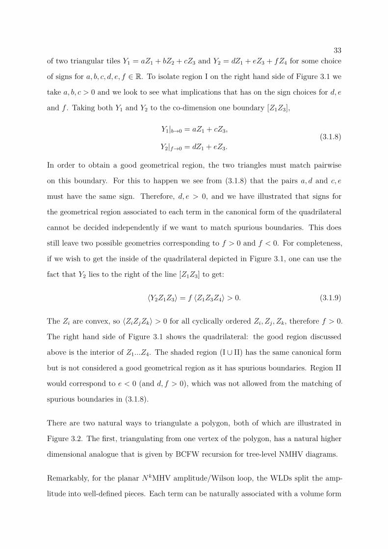
33of two triangular tiles Y1 = aZ1 + bZ2 + cZ3 and Y2 = dZ1 + eZ3 + fZ4 for some choice

of signs for a, b, c, d, e, f ∈ R. To isolate region I on the right hand side of Figure 3.1 we

take a, b, c > 0 and we look to see what implications that has on the sign choices for d, e

and f . Taking both Y1 and Y2 to the co-dimension one boundary [Z1Z3],

Y1|b→0 = aZ1 + cZ3,

Y2|f→0 = dZ1 + eZ3.

(3.1.8)

In order to obtain a good geometrical region, the two triangles must match pairwise

on this boundary. For this to happen we see from (3.1.8) that the pairs a, d and c, e

must have the same sign. Therefore, d, e > 0, and we have illustrated that signs for

the geometrical region associated to each term in the canonical form of the quadrilateral

cannot be decided independently if we want to match spurious boundaries. This does

still leave two possible geometries corresponding to f > 0 and f < 0. For completeness,

if we wish to get the inside of the quadrilateral depicted in Figure 3.1, one can use the

fact that Y2 lies to the right of the line [Z1Z3] to get:

〈Y2Z1Z3〉 = f 〈Z1Z3Z4〉 > 0. (3.1.9)

The Zi are convex, so 〈ZiZjZk〉 > 0 for all cyclically ordered Zi, Zj, Zk, therefore f > 0.

The right hand side of Figure 3.1 shows the quadrilateral: the good region discussed

above is the interior of Z1...Z4. The shaded region (I ∪ II) has the same canonical form

but is not considered a good geometrical region as it has spurious boundaries. Region II

would correspond to e < 0 (and d, f > 0), which was not allowed from the matching of

spurious boundaries in (3.1.8).

There are two natural ways to triangulate a polygon, both of which are illustrated in

Figure 3.2. The first, triangulating from one vertex of the polygon, has a natural higher

dimensional analogue that is given by BCFW recursion for tree-level NMHV diagrams.

Remarkably, for the planar NkMHV amplitude/Wilson loop, the WLDs split the amp-

litude into well-defined pieces. Each term can be naturally associated with a volume form

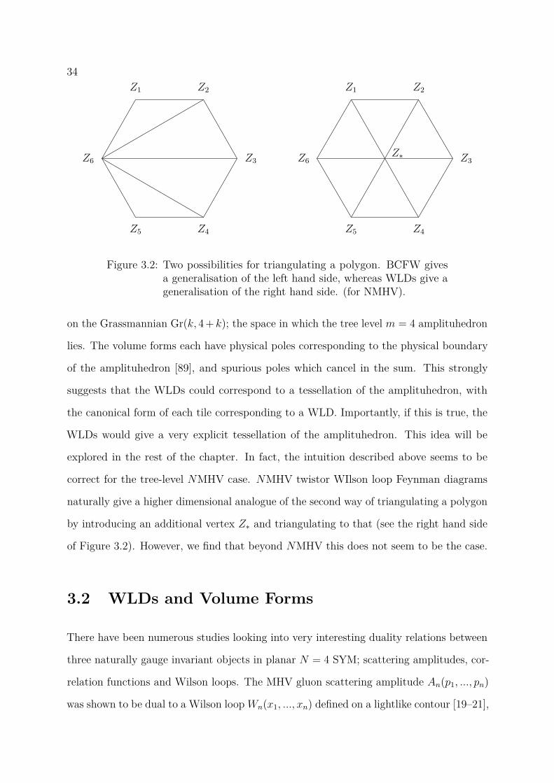
34Z2Z1

Z6

Z5 Z4

Z3

Z2Z1

Z6

Z5 Z4

Z3Z∗

Figure 3.2: Two possibilities for triangulating a polygon. BCFW givesa generalisation of the left hand side, whereas WLDs give ageneralisation of the right hand side. (for NMHV).

on the Grassmannian Gr(k, 4 + k); the space in which the tree level m = 4 amplituhedron

lies. The volume forms each have physical poles corresponding to the physical boundary

of the amplituhedron [89], and spurious poles which cancel in the sum. This strongly

suggests that the WLDs could correspond to a tessellation of the amplituhedron, with

the canonical form of each tile corresponding to a WLD. Importantly, if this is true, the

WLDs would give a very explicit tessellation of the amplituhedron. This idea will be

explored in the rest of the chapter. In fact, the intuition described above seems to be

correct for the tree-level NMHV case. NMHV twistor WIlson loop Feynman diagrams

naturally give a higher dimensional analogue of the second way of triangulating a polygon

by introducing an additional vertex Z∗ and triangulating to that (see the right hand side

of Figure 3.2). However, we find that beyond NMHV this does not seem to be the case.

3.2 WLDs and Volume Forms

There have been numerous studies looking into very interesting duality relations between

three naturally gauge invariant objects in planar N = 4 SYM; scattering amplitudes, cor-

relation functions and Wilson loops. The MHV gluon scattering amplitude An(p1, ..., pn)

was shown to be dual to a Wilson loopWn(x1, ..., xn) defined on a lightlike contour [19–21],

35by identifying the cusp points xi of the Wilson loop as the dual momenta of the particle pi

(see section 2.3). The correlation functions Gn = 〈O(x1)...O(xn)〉 of local gauge invariant

operators O(x) were shown to be dual to Wilson loops, and therefore to amplitudes, in

the light like limit limx2|i,i+1→0 x212...x

2n1Gn =Wn [25,91]. The former, [22–24], and the lat-

ter, [26–28], both have supersymmetric generalisations. We utilise the amplitude/Wilson

loop duality here in order to write the amplitude as a sum over twistor Wilson loop dia-

grams, each of which have an associated integral expression with spurious poles that cancel

when summed. These expressions will then be mapped to volume forms in amplituhedron

coordinates which we will attempt to give geometrical meaning to.

In this section, we provide a brief description of Wilson loops in N = 4 Super Yang Mills

in super-twistor space and define the related Wilson loop diagrams. We will then show

how to map the expression that arises from a WLD to a volume form in Gr(k, 4 + k), the

same space in which the amplituhedron lives.

3.2.1 Planar Wilson Loop Diagrams in N = 4 SYM

The fields of N = 4 SYM can be described by a superfield A, a (0, 1)-form on supertwistor

space (see for example [92,93]). It has an expansion in the fermionic twistor variables χA,

A = g+ + χAψA + 12χ

AχBφAB + 13!εABCDχ

AχBχCψD + 14!εABCDχ

AχBχCχDg−, (3.2.1)

where ψ and ψ are the eight fermions, the antisymmetric φ are the six scalars and g±

are the positive and negative helicity gluons. These are precisely the on-shell degrees of

freedom for N = 4 SYM. The twistor action of N = 4 SYM is given by

S [A] = i

2π

∫D3|4ZTr

(A ∧ ∂A+ 2

3A ∧A ∧A)

+ g2∫

d4|8x log det((∂ +A

)|X)

(3.2.2)

where g2 is the Yang-Mills coupling,(∂ +A

)|X restricts ∂ +A to the projective line X

in twistor space,which corresponds to the point (x, θ) in spacetime, and the integration

measure is over complex projective space D3|4Z = 14!εIJKL dZI dZJ dZK d4χ. The first

36term in the action is equivalent to holomorphic Chern-Simons theory [93, 94], and the

second term describes the interacting non self-dual part.3

To obtain the Feynman rules in twistor space, one can impose an axial gauge by choosing

a reference twistor Z∗ and insisting that the component of A in the direction of Z∗ is zero,

i.e. Z∗ · A = 0. The cubic term in (3.2.2) is zero since imposing this gauge reduces the

number of components of A from three down to two, and the first term, the kinetic term,

defines a propagator. This is known as the CSW gauge and was first introduced in [14].

The log det term can be Taylor expanded, where in this gauge each term corresponds to

an MHV amplitude. This can be expressed in twistor space and gives a Feynman diagram

formalism for amplitudes known as the “MHV diagram formalism”. For a more detailed

description of the twistor action (3.2.2) and the expansion hinted at here, see [96] and

the references therein.

The Feynman diagrams can also be used to calculate the expectation value of the polygonal

holomorphic Wilson-loop in supertwistor space, with vertices being the supertwistors

Z1...Zn ∈ C4|4. In the planar theory, this is equivalent via the Wilson loop/amplitude

duality to n-point superamplitudes. We refer to these diagrams as Wilson loop diagrams

(WLDs), and are what we are interested in going forward. Below we will discuss the

Feynman rules for these diagrams. We do not look to derive these here; for their derivation

see [23,97,98].

At tree level, the Feynman diagrams consist simply of propagators whose two ends lie on

the Wilson loop contour. In the planar theory, diagrams are only valid if we can draw

all the propagators inside the Wilson loop without crossing. The NkMHV Wilson loop is

the sum over all such diagrams involving k propagators; see Figure 3.3 for an example of

a diagram contributing to the 8-point N4MHV amplitude.

3To see motivation for the form of the log det interaction term from twistor-string theory we refer theinterested reader to [92,95]

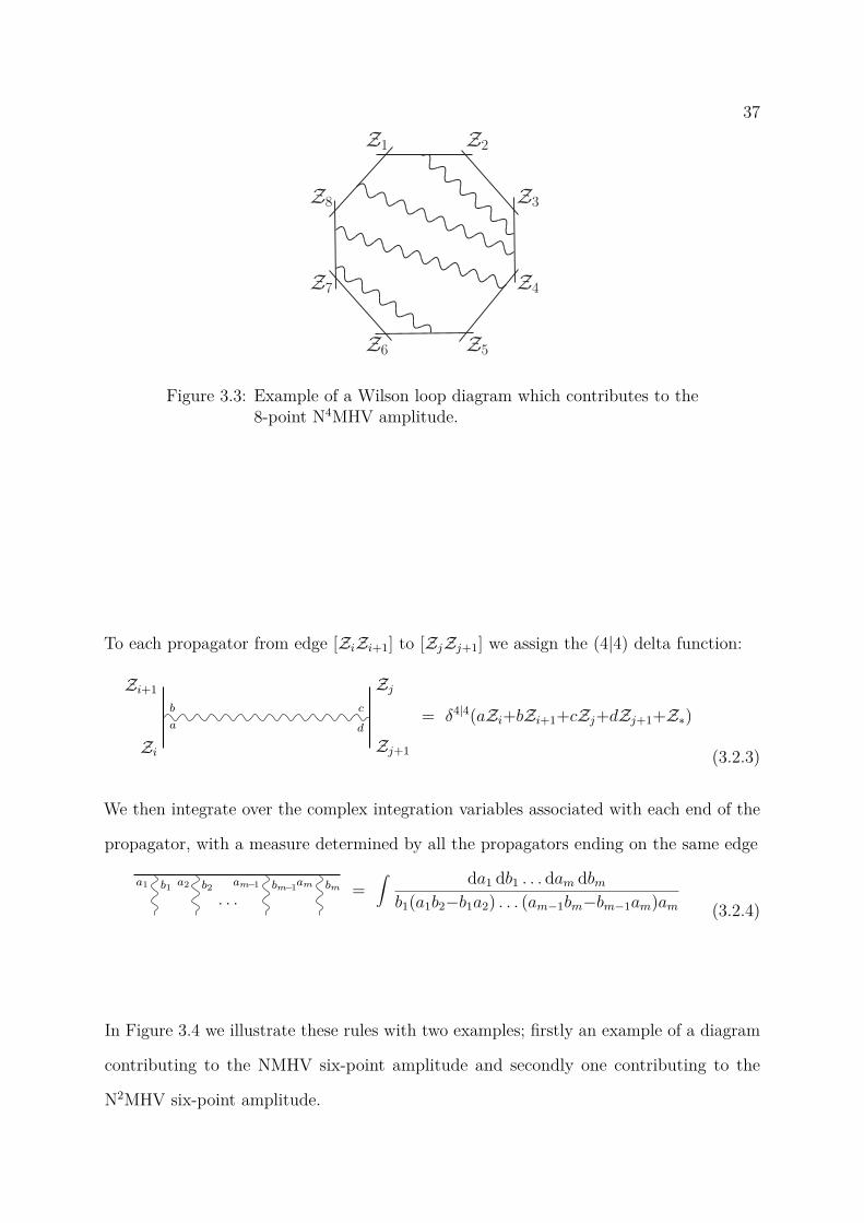
37Z1 Z2

Z3

Z4

Z5Z6

Z7

Z8

Figure 3.3: Example of a Wilson loop diagram which contributes to the8-point N4MHV amplitude.

To each propagator from edge [ZiZi+1] to [ZjZj+1] we assign the (4|4) delta function:

Zi+1

Zi

b

a

c

d

Zj

Zj+1

= δ4|4(aZi+bZi+1+cZj+dZj+1+Z∗)

(3.2.3)

We then integrate over the complex integration variables associated with each end of the

propagator, with a measure determined by all the propagators ending on the same edge

a1 b1 a2 b2 am−1 bm−1am bm

. . .=

∫ da1 db1 . . . dam dbmb1(a1b2−b1a2) . . . (am−1bm−bm−1am)am (3.2.4)

In Figure 3.4 we illustrate these rules with two examples; firstly an example of a diagram

contributing to the NMHV six-point amplitude and secondly one contributing to the

N2MHV six-point amplitude.

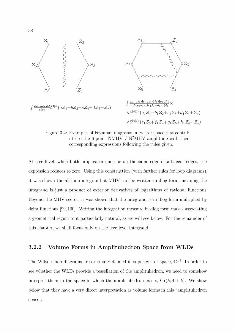
38

Z1 Z2

Z3

Z4Z5

Z6

Z1 Z2

Z3

Z4Z5

Z6

∫ dadb dcddabcd

δ4|4 (aZ1+bZ2+cZ4+dZ5+Z∗)∫ da1 db1 dc1 dd1 df1 dg1 dh1

a1b1g1h1e1(c1f1−d1e1)d1×

×δ(4|4) (a1Z1+b1Z2+c1Z3+d1Z4+Z∗)

×δ(4|4) (e1Z3+f1Z4+g1Z5+h1Z6+Z∗)

Figure 3.4: Examples of Feynman diagrams in twistor space that contrib-ute to the 6-point NMHV / N2MHV amplitude with theircorresponding expressions following the rules given.

At tree level, when both propagator ends lie on the same edge or adjacent edges, the

expression reduces to zero. Using this construction (with further rules for loop diagrams),

it was shown the all-loop integrand at MHV can be written in dlog form, meaning the

integrand is just a product of exterior derivatives of logarithms of rational functions.

Beyond the MHV sector, it was shown that the integrand is in dlog form multiplied by

delta functions [99, 100]. Writing the integration measure in dlog form makes associating

a geometrical region to it particularly natural, as we will see below. For the remainder of

this chapter, we shall focus only on the tree level integrand.

3.2.2 Volume Forms in Amplituhedron Space from WLDs

The Wilson loop diagrams are originally defined in supertwistor space, C4|4. In order to

see whether the WLDs provide a tessellation of the amplituhedron, we need to somehow

interpret them in the space in which the amplituhedron exists, Gr(k, 4 + k). We show

below that they have a very direct interpretation as volume forms in this “amplituhedron

space”.

39Following their description in the previous section, we saw that all NkMHV WLDs have

the general form

∫Ω4k (ai) δk×(4|4) (C (ai) .Z) [WLD]. (3.2.5)

The variables in (3.2.5) are defined as follows,

• ai: the 4k coordinates, four for each of the k propagators of the WLD.

• Z: the external particles in supertwistor space, organised as the rows of an (n +

1)× (4|4) matrix.

• Ω4k (ai): the integration measure. A 4k-form consisting of a product of terms of the

form (3.2.4).

• δk×(4|4) (C (ai) .Z): the k delta functions, one for each propagator, written as a

k × (n+ 1) matrix of the coordinates, C(ai), acting on the external supertwistors

Z.

We now look to interpret (3.2.5) as a canonical form in the amplituhedron space. This

can be done straightforwardly via the map

Ω(Y ) = Ω4k(ai) Y = C(ai).Z ∈ Gr(k, k + 4). (3.2.6)

The coordinates are now reinterpreted as coordinates in Gr(k, k + 4), and the Z here

is the (n + 1) × (4 + k) matrix with each row corresponding to an external momentum

supertwistor now bosonised in the way described in section 2.3.

We once again turn to the two examples in Figure 3.4 to illustrate this point. For the

NMHV diagram, the volume form in amplituhedron space can be read off:

∫ dadb dc ddabcd

δ4|4 (aZ1+bZ2+cZ4+dZ5+Z∗) [WLD]

↓

Ω = da db dcddabcd

Y = aZ1+bZ2+cZ4+dZ5+Z∗ ∈ C5 [Amplituhedron Volume form]

(3.2.7)

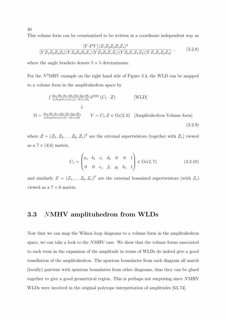
40This volume form can be covariantised to be written in a coordinate independent way as

〈Y d4Y 〉〈Z1Z2Z4Z5Z∗〉4

〈Y Z1Z2Z4Z5〉〈Y Z2Z4Z5Z∗〉〈Y Z4Z5Z∗Z1〉〈Y Z5Z∗Z1Z2〉〈Y Z∗Z1Z2Z4〉, (3.2.8)

where the angle brackets denote 5× 5 determinants.

For the N2MHV example on the right hand side of Figure 3.4, the WLD can be mapped

to a volume form in the amplituhedron space by

∫ da1 db1 dc1 dd1 df1 dg1 dh1a1b1g1h1e1(c1f1−d1e1)d1

δ(8|8) (C1 · Z) [WLD]

↓

Ω = da1 db1 dc1 dd1 df1 dg1 dh1a1b1g1h1e1(c1f1−d1e1)d1

Y = C1.Z ∈ Gr(2, 6) [Amplituhedron Volume form]

(3.2.9)

where Z = (Z1,Z2, . . .Z6,Z∗)T are the external supertwistors (together with Z∗) viewed

as a 7× (4|4) matrix,

C1 =

a1 b1 c1 d1 0 0 1

0 0 e1 f1 g1 h1 1

∈ Gr(2, 7) (3.2.10)

and similarly Z = (Z1, . . . Z6, Z∗)T are the external bosonised supertwistors (with Z∗)

viewed as a 7× 6 matrix.

3.3 NMHV amplituhedron from WLDs

Now that we can map the Wilson loop diagrams to a volume form in the amplituhedron

space, we can take a look to the NMHV case. We show that the volume forms associated

to each term in the expansion of the amplitude in terms of WLDs do indeed give a good

tessellation of the amplituhedron. The spurious boundaries from each diagram all match

(locally) pairwise with spurious boundaries from other diagrams, thus they can be glued

together to give a good geometrical region. This is perhaps not surprising since NMHV

WLDs were involved in the original polytope interpretation of amplitudes [63, 74].

413.3.1 Cancellation of spurious poles in NMHV WLDs

The n-point NMHV amplitude in the twistor Wilson loop description is given by a sum

over all diagrams with a single propagator attached to any two edges of the polygon. The

diagram with a propagator which has ends attached to the edges [ZiZi+1] and [ZjZj+1]

can be associated to the volume form in Gr(1, 5)

Ω = da db dc ddabcd

Y = aZi+bZi+1+cZj+dZj+1+Z∗ ∈ C5. (3.3.1)

Writing this in a coordinate independent form as in (3.2.8) gives

〈Y d4Y 〉〈ZiZi+1ZjZj+1Z∗〉4

〈Y ZiZi+1ZjZj+1〉〈Y Zi+1ZjZj+1Z∗〉〈Y ZjZj+1Z∗Zi〉〈Y Zj+1Z∗ZiZi+1〉〈Y Z∗ZiZi+1Zj〉.

(3.3.2)

The full NMHV amplitude is given by summing over all positions of the ends of the

propagator,

Ω = 〈Y d4Y 〉

×∑i<j

〈ZiZi+1ZjZj+1Z∗〉4

〈Y ZiZi+1ZjZj+1〉〈Y Zi+1ZjZj+1Z∗〉〈Y ZjZj+1Z∗Zi〉〈Y Zj+1Z∗ZiZi+1〉〈Y Z∗ZiZi+1Zj〉,

(3.3.3)

where requiring i < j comes from the fact that the diagrams are invariant under the

swapping of the two propagator ends.

Looking at (3.3.1), it is clear that the spurious poles for each WLD arise when any one of

a, b, c, d→ 0. There is another pole present when a, b, c, d→∞ simultaneously, however

this is a physical pole of the amplitude and does not cancel in the sum over the diagrams.

From the point of view of the WLDs, the spurious poles occur when one end of the

propagator approaches a vertex. However, this spurious pole is cancelled when the WLD

is added together with a neighbouring diagram, where the propagator approaches the

same vertex but from the adjacent edge. This is illustrated in Figure 3.5.

Algebraically this cancellation is straightforward, but for completeness we shall show it

42

Figure 3.5: Spurious poles occur when the propagator end reaches thevertex. It is cancelled by the adjacent diagram.

explicitly for the diagrams in Figure 3.5. Using the rules from section 3.2.1, the integrals

associated to the two diagrams are

I (DL) =∫ da1 db1 dc1 dd1

a1b1c1d1δ4|4 (CL · Z) (3.3.4)

and

I (DR) =∫ da2 db2 dc2 dd2

a2b2c2d2δ4|4 (CR · Z) . (3.3.5)

The corresponding 1× (n+ 1) C matrices are given by

CL =(· · · a1 b1 · · · c1 d1 0 · · · 1

), (3.3.6)

CR =(· · · a2 b2 · · · 0 c2 d2 · · · 1

), (3.3.7)

where the entries explicitly written out in both matrices are the i, i+ 1, j, j + 1, j + 2 and

n+ 1 entries, with all other entries being 0.

The spurious poles being discussed here occur when c1 → 0 and d2 → 0, and the claim

more precisely is that in summing the two diagrams the residues at these poles precisely

cancel

Resc1=0I(DL) + Res

d2=0I(DR) = 0. (3.3.8)

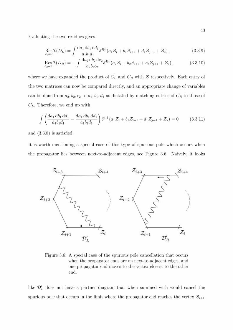
43Evaluating the two residues gives

Resc1=0I(DL) =

∫ da1 db1 dd1

a1b1d1δ4|4 (a1Zi + b1Zi+1 + d1Zj+1 + Z∗) , (3.3.9)

Resd2=0I(DR) = −

∫ da2 db2 dc2

a2b2c2δ4|4 (a2Zi + b2Zi+1 + c2Zj+1 + Z∗) , (3.3.10)

where we have expanded the product of CL and CR with Z respectively. Each entry of

the two matrices can now be compared directly, and an appropriate change of variables

can be done from a2, b2, c2 to a1, b1, d1 as dictated by matching entries of CR to those of

CL. Therefore, we end up with

∫ (da1 db1 dd1

a1b1d1− da1 db1 dd1

a1b1d1

)δ4|4 (a1Zi + b1Zi+1 + d1Zj+1 + Z∗) = 0 (3.3.11)

and (3.3.8) is satisfied.

It is worth mentioning a special case of this type of spurious pole which occurs when

the propagator lies between next-to-adjacent edges, see Figure 3.6. Naively, it looks

Figure 3.6: A special case of the spurious pole cancellation that occurswhen the propagator ends are on next-to-adjacent edges, andone propagator end moves to the vertex closest to the otherend.

like D′L does not have a partner diagram that when summed with would cancel the

spurious pole that occurs in the limit where the propagator end reaches the vertex Zi+1.

44Following previous considerations, the partner diagram would have propagator ends lying

on adjacent edges, but this diagram vanishes. Instead, it pairs with the diagram with

propagator ends on edge [Zi+1Zi+2] and [Zi+3Zi+4], illustrated by D′R in Figure 3.6. The

expressions for this pair of WLDs are given by

I(D′L) =∫ da1 db1 dc1 dd1

a1b1c1d1δ4|4 (a1Zi + b1Zi+1 + c1Zi+2 + d1Zi+3 + Z∗) , (3.3.12)

I(D′R) =∫ da2 db2 dc2 dd2

a2b2c2d2δ4|4 (a2Zi+1 + b2Zi+2 + c2Zi+3 + d2Zi+4 + Z∗) , (3.3.13)

and the relation for this special case is given by

Resa1=0I(D′L) + Res

d2=0I(D′R) = 0. (3.3.14)

3.3.2 Spurious boundary matching

There is a natural geometrical interpretation of the NMHV amplitude as a union of tiles,

each giving one of the terms in (3.3.3) as its canonical form. This corresponds to

⋃i,j

Y = aZi+bZi+1+cZj+dZj+1+Z∗ ; a, b, c, d ≥ 0 ⊂ Gr(1, 5) . (3.3.15)

It should be noted that the variables (a, b, c, d) used to describe the geometrical region in

(3.3.15) are the same variables given by the WLDs, (3.3.1). The WLD integration is over

complex space, however here the variables are restricted to a subspace of the real line.

If 〈ZiZjZkZlZm〉 > 0 for all cyclically ordered Zi, Zj, Zk, Zl, Zm, corresponding to the

Z’s being convex, then (3.3.15) provides a tessellation of the amplituhedron as defined

in [47]. This is the higher dimensional generalisation of the triangulation of the polygon

in the toy model illustrated on the right hand side of Figure 3.2. In fact, this defines a

good geometrical region, meaning one without spurious boundaries, even for non-convex

choices of external kinematic data Zi.

Motivated by the toy example discussed around Figure 3.1, it is interesting to determine

how unique this region is. Any choice of signs for the variables a, b, c, d in each tile will

associate the same canonical form to each WLD. However, as we saw for the quadrilateral,

45choosing arbitrary signs for each tile independently could lead to a geometrical region

which still has spurious boundaries left over even though the spurious poles in the sum

of the corresponding canonical forms do cancel. Imposing that this cancellation of poles

has a corresponding geometric meaning as a matching of spurious boundaries gives a

correlation between the sign choices for the geometric image of the tiles.

To begin exploring whether other good geometrical regions can be determined from the

canonical forms of the WLDs, let us consider a particular tile corresponding to the WLD

with a propagator from edge [ZiZi+1] to edge [ZjZj+1]. The most general geometry giving

(3.3.1,3.3.2) as its canonical form is

Y = asiZi+bsi+1Zi+1+csjZj+dsj+1Zj+1+Z∗ : a, b, c, d ≥ 0, (3.3.16)

where si, si+1, sj, sj+1 = ±1 are four arbitrary sign choices. Recalling the location of the

spurious poles discussed in the previous section, the associated spurious boundaries arise

when any one of the four coordinates a, b, c, d→ 0 (while a physical boundary occurring

when simultaneously a, b, c, d → ∞). Focussing on the spurious boundary a → 0, and

motivated by the fact the related spurious pole cancels by summing with a neighbouring

diagram, this boundary must match the boundary when b→ 0 of the adjacent diagram

with a propagator from edge [Zi+1Zi+2] to edge [ZjZj+1]. Defining arbitrary signs for the

neighbouring diagram, s′i+1, s′i+2, s

′j, s′j+1 = ±1, we have

Y = asiZi+bsi+1Zi+1+csjZj+dsj+1Zj+1+Z∗ : a = 0, b, c, d ≥ 0

=

Y = as′i+1Zi+1+bs′i+2Zi+2+cs′jZj+ds′j+1Zj+1+Z∗ : b = 0, a, c, d ≥ 0.

(3.3.17)

This boundary matching mimics the spurious pole cancellation in Figure 3.5 and sur-

rounding discussion. Comparing the two regions and imposing that these two spurious

boundaries match, we find a set of consistency conditions on the sign choices of the two

tiles:

si+1 = s′i+1, sj = s′j, sj+1 = s′j+1. (3.3.18)

46So, the signs associated with each vertex for different diagrams must be the same. Of

course, very similar considerations can be applied for the other spurious boundaries that

occur when b, c or d→ 0

One can continue this discussion for the spurious poles of all NMHV diagrams, moving

the propagator around the edges of the polygon and fixing signs by comparing expressions

similar to (3.3.17) at each step. In doing so, we see that the region

⋃i,j

Y = asiZi+bsi+1Zi+1+csjZj+dsj+1Zj+1+Z∗ ; a, b, c, d ≥ 0 ⊂ Gr(1, 5) (3.3.19)

is the most general geometry matching the WLDs that has no spurious boundaries, which

can be obtained by assigning a fixed sign si = ±1 to each vertex Zi. This is equivalent

to considering the original amplituhedron with all positive signs but flipping the sign of

the external Z’s. Note that at most one choice of signs for the Zs can correspond to a

convex shape).

Naively, one may think that a more general possibility could have existed, consisting of

assigning two sets of fixed signs per vertex rather than one, corresponding to one set per

propagator end. However, in starting from one diagram and moving the propagator round

the polygon, matching spurious boundaries as you go, eventually the same diagram is

reached that you started on with the propagator ends switched. This reversed propagator

has to correspond to the same geometrical region as the original, therefore the two sets

of signs must in fact be equal to each other.

To complete the discussion of spurious boundaries for the NMHV case, it is worth double

checking that this general geometrical region (3.3.19) is consistent with the special case of

spurious pole cancellation illustrated in Figure 3.6 and the discussion around it. For this

particular example, the geometry associated to the diagram with a propagator between

edge [ZiZi+1] and edge [Zi+2Zi+3] should match along the spurious boundary that occurs

when a = 0 with the diagram with a propagator between edge [Zi+1Zi+2] and edge

47[Zi+3Zi+4] along the boundary that occurs when d = 0. We get

Y = asiZi+bsi+1Zi+1+csi+2Zi+2+dsi+3Zi+3+Z∗ ; a = 0, b, c, d ≥ 0

=

Y = asi+1Zi+1+bsi+2Zi+2+csi+3Zi+3+dsi+4Zi+4+Z∗ ; d = 0, a, b, c ≥ 0 ,

(3.3.20)

and see that indeed the spurious boundaries do match for this special case too, even for

the general choice of signs.

3.4 N 2MHV

Having discussed how to obtain a “good” geometry from the WLDs for NMHV, we now

look to the next highest helicity degree. We will begin by discussing new spurious poles

that occur at N2MHV, and show how they cancel algebraically. We will then prove that

beyond NMHV the WLDs cannot be glued together to form a geometry without spurious

boundaries. To do this, we show that this is no set of sign choices for the coordinates

of each tile that is consistent with the pairwise matching of spurious boundaries. Note,

by pairwise matching we mean locally; there could by more than two diagrams involved

in the matching of a spurious boundary. In fact, we will see this during the discussions

that follow. In order to illustrate the argument we will focus on the case of n = 6 in the

coming sections, however we emphasise that the argument is easily generalised to all n.

3.4.1 Cancellation of spurious poles in N 2MHV WLDs

To begin, we consider the algebraic cancellation of spurious poles for N2MHV diagrams.

The discussion from Section 3.3.1 involving the spurious pole that occurs when a propag-

ator end approaches a vertex still holds for any MHV degree. However, from N2MHV

a new spurious pole occurs; now that we have more than one propagator, there is the

possibility that two propagator ends come together, which produces a pole in the in-

tegral of the WLD. Unlike the previous type of pole, there is an interesting three-way

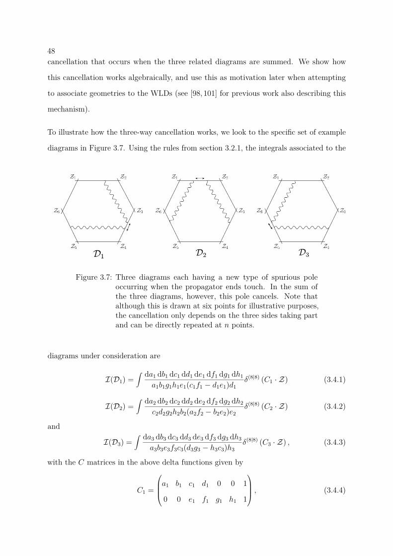
48cancellation that occurs when the three related diagrams are summed. We show how

this cancellation works algebraically, and use this as motivation later when attempting

to associate geometries to the WLDs (see [98, 101] for previous work also describing this

mechanism).

To illustrate how the three-way cancellation works, we look to the specific set of example

diagrams in Figure 3.7. Using the rules from section 3.2.1, the integrals associated to the

Figure 3.7: Three diagrams each having a new type of spurious poleoccurring when the propagator ends touch. In the sum ofthe three diagrams, however, this pole cancels. Note thatalthough this is drawn at six points for illustrative purposes,the cancellation only depends on the three sides taking partand can be directly repeated at n points.

diagrams under consideration are

I(D1) =∫ da1 db1 dc1 dd1 de1 df1 dg1 dh1

a1b1g1h1e1(c1f1 − d1e1)d1δ(8|8) (C1 · Z) (3.4.1)

I(D2) =∫ da2 db2 dc2 dd2 de2 df2 dg2 dh2

c2d2g2h2b2(a2f2 − b2e2)e2δ(8|8) (C2 · Z) (3.4.2)

and

I(D3) =∫ da3 db3 dc3 dd3 de3 df3 dg3 dh3

a3b3e3f3c3(d3g3 − h3c3)h3δ(8|8) (C3 · Z) , (3.4.3)

with the C matrices in the above delta functions given by

C1 =

a1 b1 c1 d1 0 0 1

0 0 e1 f1 g1 h1 1

, (3.4.4)

49

C2 =

a2 b2 0 0 c2 d2 1

e2 f2 g2 h2 0 0 1

, (3.4.5)

C3 =

a3 b3 0 0 c3 d3 1

0 0 e3 f3 g3 h3 1

. (3.4.6)

Each expression clearly has a pole at the point corresponding to the propagator ends

coinciding (i.e. c1f1 = d1e1 for the first case, a2f2 = b2e2 for the second and d3g3 = h3c3

for the third).

The claim is that in summing the diagrams, the residues at these poles precisely cancel:

Resc1f1=d1e1

I(D1) + Resa2f2=b2e2

I(D2) + Resd3g3=h3c3

I(D3) = 0. (3.4.7)

In order to show this, it is useful to change variables in the following way:

(e1, f1)→ (α, ε1) (e2, f2)→ (β, ε2) (g3, h3)→ (γ, ε3)

e1 = αc1, f1 = αd1 + ε1 e2 = βa2, f2 = βb2 + ε2 g3 = γc3 + ε3, h3 = γd3

The spurious poles in question now occur when ε1, ε2, ε3 → 0. Substituting these new

variables into the integrals corresponding to the WLDs currently being examined gives

Resε1=0I(D2) = Res

ε1=0

∫ da1 db1 dc1 dd1 dg1 dh1 dα dε1a1b1c1d1g1h1αε1

δ(8|8) (C1 · Z)

=∫ da1 db1 dc1 dd1 dg1 dh1 dα

a1b1c1d1g1h1αδ(8|8) (C1|ε1=0 · Z) , (3.4.8)

Resε2=0I(D1) = Res

ε2=0

∫ da2 db2 dc2 dd2 dg2 dh2 dβ dε2a2b2c2d2g2h2βε2

δ(8|8) (C2 · Z)

=∫ da2 db2 dc2 dd2 dg2 dh2 dβ

a2b2c2d2g2h2βδ(8|8) (C2|ε2=0 · Z) (3.4.9)

and

Resε3=0I(D3) = Res

ε3=0−∫ da3 db3 dc3 dd3 de3 df3 dγ dε3

a3b3c3d3e3f3γε3δ(8|8) (C3 · Z)

= −∫ da3 db3 dc3 dd3 de3 df3 dγ

a3b3c3d3e3f3γδ(8|8) (C3|ε3=0 · Z) . (3.4.10)

The measure in each expression is now simply the dlog of all the variables. The associated

50C matrices in the delta functions become

C1|ε1=0 =

a1 b1 c1 d1 0 0 1

0 0 αc1 αd1 g1 h1 1

, (3.4.11)

C2|ε2=0 =

a2 b2 0 0 c2 d2 1

βa2 βb2 g2 h2 0 0 1

(3.4.12)

and

C3|ε3=0 =

a3 b3 0 0 c3 d3 1

0 0 e3 f3 γc3 γd3 1

. (3.4.13)

In order to compare the three Ci ∈ GR(2, 7), we must introduce a change of parameteriz-

ation. Utilising the GL(2) invariance, we make the following change of basis for C2 and

C3,

C ′2 =

0 1−β1−β

11−β

C2 (3.4.14)

and

C ′3 =

−γ1−γ

11−γ

0 1

C3. (3.4.15)

The three matrices C1, C′2 and C ′3 are now of the same form, meaning they have zeros and

ones in the same entries and variables in the others:

C ′2 =

βa2 βb2 g2 h2 0 0 1

0 0 g21−β

h21−β

−βc21−β

−βd21−β 1

, (3.4.16)

C ′3 =

−γa31−γ

−γb31−γ

e31−γ

f31−γ 0 0 1

0 0 e3 f3 γc3 γd3 1

. (3.4.17)

We continue in a similar way to the simpler spurious pole discussed in Section 3.3.1 by

comparing each entry in C ′2 and C ′3 directly to the equivalent entry in C1. We make a

change of variables for C ′2 and C ′3 to the variables of C1 as dictated by matching entries:

C ′2 :a2 → α

α−1a1 b2 → αα−1b1 g2 → c1

h2 → d1 c2 → 11−αg1 d2 → 1

1−αh1

β → −(1− α)α

, (3.4.18)

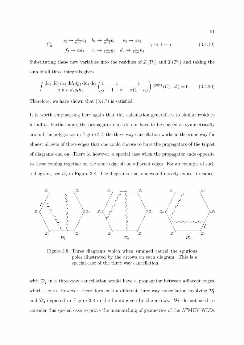
51

C ′3 :a3 → α

α−1a1 b3 → αα−1b1 e3 → αc1

f3 → αd1 c3 → 11−αg1 d3 → 1

1−αh1

γ → 1− α. (3.4.19)

Substituting these new variables into the residues of I (D2) and I (D3) and taking the

sum of all three integrals gives

∫ da1 db1 dc1 dd1dg1 dh1 dαa1b1c1d1g1h1

(1α

+ 11− α −

1α(1− α)

)δ(8|8) (C1 · Z) = 0. (3.4.20)

Therefore, we have shown that (3.4.7) is satisfied.

It is worth emphasising here again that this calculation generalises to similar residues

for all n. Furthermore, the propagator ends do not have to be spaced as symmetrically

around the polygon as in Figure 3.7; the three way cancellation works in the same way for

almost all sets of three edges that one could choose to have the propagators of the triplet

of diagrams end on. There is, however, a special case when the propagator ends opposite

to those coming together on the same edge sit on adjacent edges. For an example of such

a diagram, see D′2 in Figure 3.8. The diagrams that one would naively expect to cancel

Figure 3.8: Three diagrams which when summed cancel the spuriouspoles illustrated by the arrows on each diagram. This is aspecial case of the three way cancellation.

with D′2 in a three-way cancellation would have a propagator between adjacent edges,

which is zero. However, there does exist a different three-way cancellation involving D′1and D′3 depicted in Figure 3.8 in the limits given by the arrows. We do not need to

consider this special case to prove the mismatching of geometries of the N2MHV WLDs

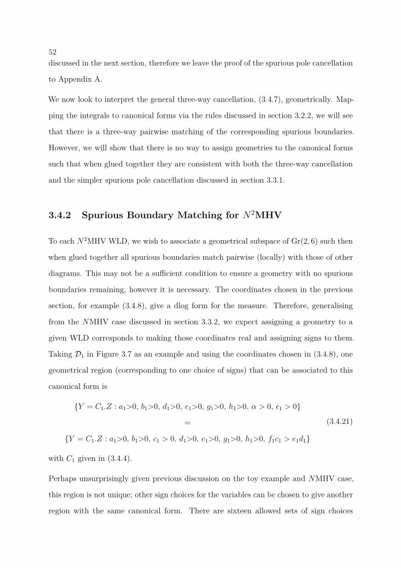
52discussed in the next section, therefore we leave the proof of the spurious pole cancellation

to Appendix A.

We now look to interpret the general three-way cancellation, (3.4.7), geometrically. Map-

ping the integrals to canonical forms via the rules discussed in section 3.2.2, we will see

that there is a three-way pairwise matching of the corresponding spurious boundaries.

However, we will show that there is no way to assign geometries to the canonical forms

such that when glued together they are consistent with both the three-way cancellation

and the simpler spurious pole cancellation discussed in section 3.3.1.

3.4.2 Spurious Boundary Matching for N 2MHV

To each N2MHV WLD, we wish to associate a geometrical subspace of Gr(2, 6) such then

when glued together all spurious boundaries match pairwise (locally) with those of other

diagrams. This may not be a sufficient condition to ensure a geometry with no spurious

boundaries remaining, however it is necessary. The coordinates chosen in the previous

section, for example (3.4.8), give a dlog form for the measure. Therefore, generalising

from the NMHV case discussed in section 3.3.2, we expect assigning a geometry to a

given WLD corresponds to making those coordinates real and assigning signs to them.

Taking D1 in Figure 3.7 as an example and using the coordinates chosen in (3.4.8), one

geometrical region (corresponding to one choice of signs) that can be associated to this

canonical form is

Y = C1.Z : a1>0, b1>0, d1>0, e1>0, g1>0, h1>0, α > 0, ε1 > 0

=

Y = C1.Z : a1>0, b1>0, c1 > 0, d1>0, e1>0, g1>0, h1>0, f1c1 > e1d1

(3.4.21)

with C1 given in (3.4.4).

Perhaps unsurprisingly given previous discussion on the toy example and NMHV case,

this region is not unique; other sign choices for the variables can be chosen to give another

region with the same canonical form. There are sixteen allowed sets of sign choices

53altogether. One must be careful here as the propagator ends that are on the same edge

cannot cross; the geometrical region must respect this. The eight allowed possibilities for

the parameters of these ends, c1, d1, e1, f1, can be seen in the following way. Choosing signs

s1, s2 for d1 and e1 gives four of the possibilities immediately. However, we also require

(c1f1 − e1d1) > 0: this splits each of the four cases into two disconnected regions given

by c1, f1 > 0 and c1, f1 < 0, giving the expected total of eight cases. These cases can also

be read off directly from the parametrisation of the WLD if one considers the parameters

being real instead of complex. For the ends not to cross we need either 0 < d1c1< f1

e1or

0 < e1f1< c1

d1. Choosing signs for d1, e1 gives the same eight cases as above.

In order to start our investigation of a possible geometrical region of N2MHV WLDs, we

look to the geometric interpretation of the three way cancellation described in the previous

section to give some insight. To do this, we compare the C matrices in the appropriate

limit after they have been rotated to match entries with each other, i.e. C1, C′2, C

′3, given

by

C1|ε1=0 =

a1 b1 c1 d1 0 0 1

0 0 αc1 αd1 g1 h1 1

(3.4.22)

C ′2|ε2=0 =

βa2 βb2 g2 h2 0 0 1

0 0 g21−β

h21−β

−βc21−β

−βd21−β 1

(3.4.23)

C ′3|ε3=0 =

−γa31−γ

−γb31−γ

e31−γ

f31−γ 0 0 1

0 0 e3 f3 γc3 γd3 1

. (3.4.24)

We have α = 11−β and α = 1 − γ at points where the regions touch. Using this as

motivation, we choose signs (positive or negative) for α, β and γ such that locally α, β(α)

and γ(α) share boundaries pairwise. There are two different cases that arise from this

consideration:

1. One of the variables is positive and the other two negative. Without loss of generality

we consider α > 0, β, γ < 0.

2. α, β and γ are all positive.

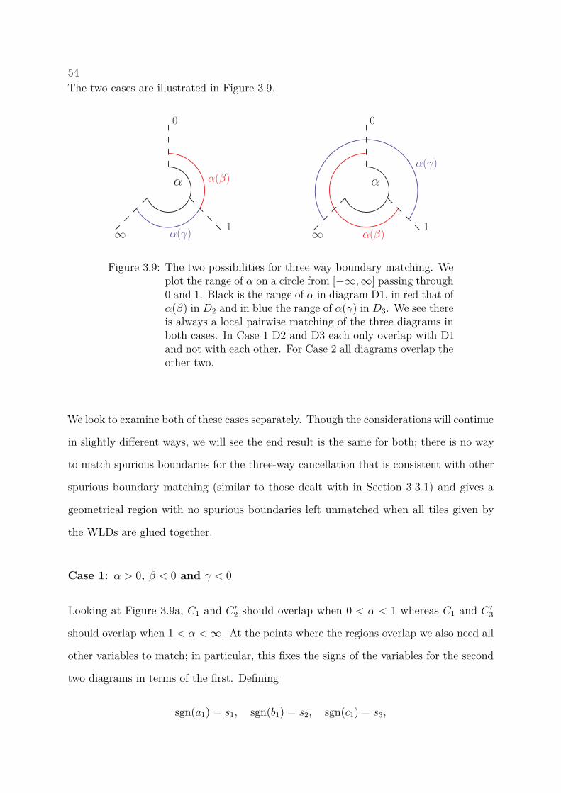
54The two cases are illustrated in Figure 3.9.

α(β)

α(γ)

0

1∞

α

0

1∞

α α(β)

α(γ)

Figure 3.9: The two possibilities for three way boundary matching. Weplot the range of α on a circle from [−∞,∞] passing through0 and 1. Black is the range of α in diagram D1, in red that ofα(β) in D2 and in blue the range of α(γ) in D3. We see thereis always a local pairwise matching of the three diagrams inboth cases. In Case 1 D2 and D3 each only overlap with D1and not with each other. For Case 2 all diagrams overlap theother two.

We look to examine both of these cases separately. Though the considerations will continue

in slightly different ways, we will see the end result is the same for both; there is no way

to match spurious boundaries for the three-way cancellation that is consistent with other

spurious boundary matching (similar to those dealt with in Section 3.3.1) and gives a

geometrical region with no spurious boundaries left unmatched when all tiles given by

the WLDs are glued together.

Case 1: α > 0, β < 0 and γ < 0

Looking at Figure 3.9a, C1 and C ′2 should overlap when 0 < α < 1 whereas C1 and C ′3should overlap when 1 < α <∞. At the points where the regions overlap we also need all

other variables to match; in particular, this fixes the signs of the variables for the second

two diagrams in terms of the first. Defining

sgn(a1) = s1, sgn(b1) = s2, sgn(c1) = s3,

55

sgn(d1) = s4, sgn(g1) = s5, sgn(h1) = s6, (3.4.25)

and comparing (3.4.23) and (3.4.24) to (3.4.22), we end up with a matrix of signs for C ′2and C ′3:

sgn(C ′2)|ε2=0 =

−s1 −s2 s3 s4 0 0 1

0 0 s3 s4 s5 s6 1

, (3.4.26)

sgn(C ′3)|ε3=0 =

s1 s2 s3 s4 0 0 1

0 0 s3 s4 −s5 −s6 1

. (3.4.27)

Undoing the GL(2) transformations, we end up with matrices giving signs for each entry

of the original C matrices:

sgn(C1)|ε1=0 =

s1 s2 s3 s4 0 0 1

0 0 s3 s4 s5 s6 1

, (3.4.28)

sgn(C2)|ε2=0 =

−s1 −s2 0 0 s5 s6 1

s1 s2 s3 s4 0 0 1

, (3.4.29)

sgn(C3)|ε3=0 =

s1 s2 0 0 −s5 −s6 1

0 0 s3 s4 s5 s6 1

. (3.4.30)

Given a set of signs for C1, the three way cancellation fixes the signs of all entries of C2

and C3 for this choice of signs for α, β and γ. Crucially, despite the signs being derived by

looking at their values at the spurious boundary, the signs remain unchanged inside the

region away from the boundary. The only subtlety occurs with those entries depending

on εi. We look to D1 in Figure 3.7 to illustrate this subtlety, with corresponding matrix

(3.4.22).

In dealing with the three way cancellation above, we fixed signs for all variables of C1

except for ε1, as it was set to zero in the limit of the propagator ends coming together.

However, away from this boundary its sign must be taken into account. In order to assign

a geometrical region to this WLD, that has a canonical form given by the dlog form in

the first line of (3.4.8), we must have a definite sign for ε1. Letting sε1 = ±1 be the sign

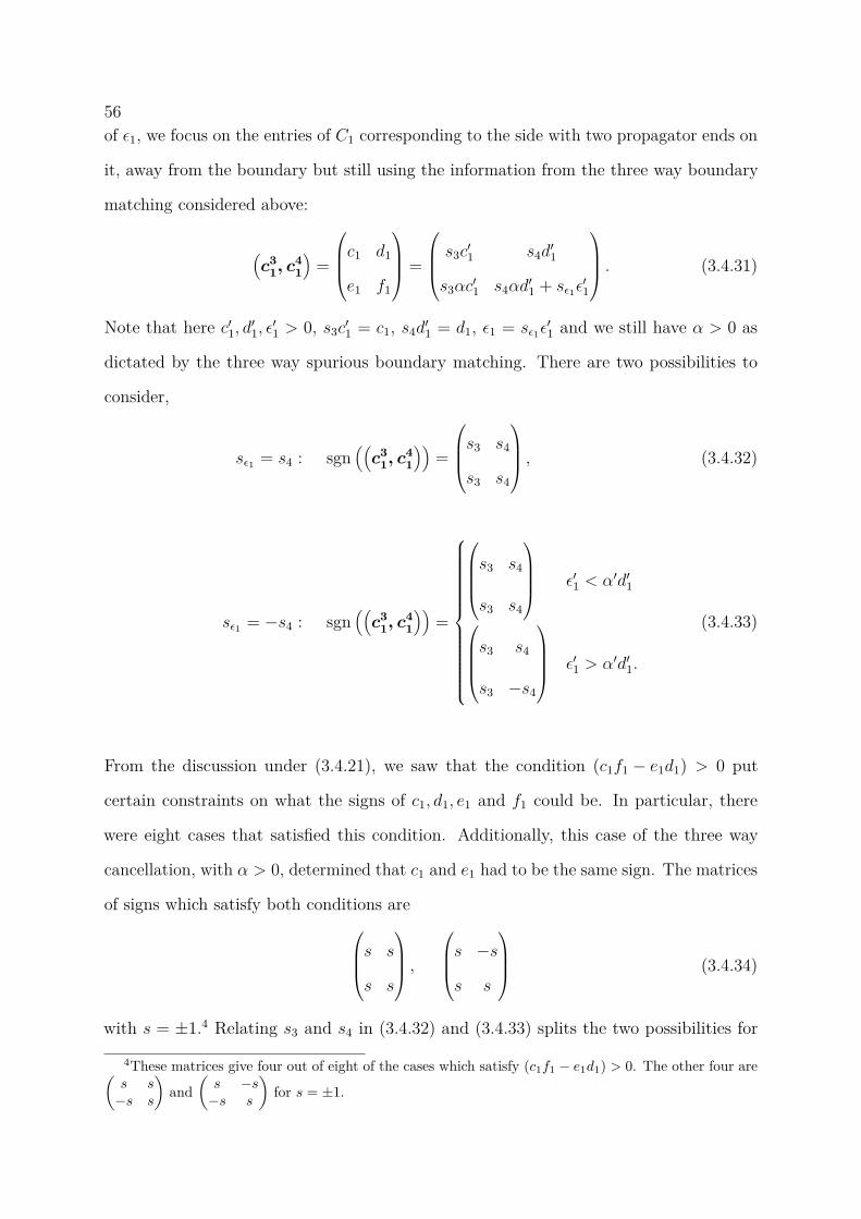
56of ε1, we focus on the entries of C1 corresponding to the side with two propagator ends on

it, away from the boundary but still using the information from the three way boundary

matching considered above:

(c3

1, c41

)=

c1 d1

e1 f1

=

s3c′1 s4d

′1

s3αc′1 s4αd

′1 + sε1ε

′1

. (3.4.31)

Note that here c′1, d′1, ε′1 > 0, s3c′1 = c1, s4d

′1 = d1, ε1 = sε1ε

′1 and we still have α > 0 as

dictated by the three way spurious boundary matching. There are two possibilities to

consider,

sε1 = s4 : sgn((

c31, c4

1

))=

s3 s4

s3 s4

, (3.4.32)

sε1 = −s4 : sgn((

c31, c4

1

))=

s3 s4

s3 s4

ε′1 < α′d′1

s3 s4

s3 −s4

ε′1 > α′d′1.

(3.4.33)

From the discussion under (3.4.21), we saw that the condition (c1f1 − e1d1) > 0 put

certain constraints on what the signs of c1, d1, e1 and f1 could be. In particular, there

were eight cases that satisfied this condition. Additionally, this case of the three way

cancellation, with α > 0, determined that c1 and e1 had to be the same sign. The matrices

of signs which satisfy both conditions ares s

s s

,s −ss s

(3.4.34)

with s = ±1.4 Relating s3 and s4 in (3.4.32) and (3.4.33) splits the two possibilities for

4These matrices give four out of eight of the cases which satisfy (c1f1 − e1d1) > 0. The other four are(s s−s s

)and

(s −s−s s

)for s = ±1.

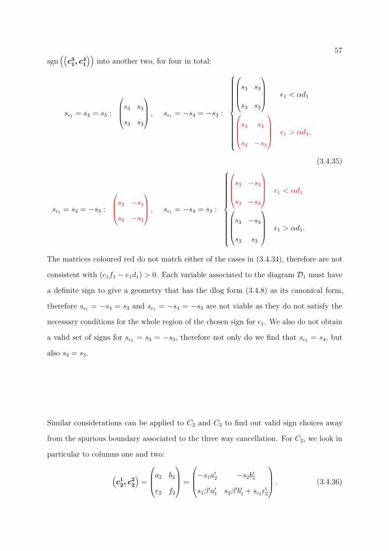
57sgn

((c3

1, c41

))into another two, for four in total:

sε1 = s4 = s3 :

s3 s3

s3 s3

, sε1 = −s4 = −s3 :

s3 s3

s3 s3

ε1 < αd1

s3 s3

s3 −s3

ε1 > αd1,

sε1 = s4 = −s3 :

s3 −s3

s3 −s3

, sε1 = −s4 = s3 :

s3 −s3

s3 −s3

ε1 < αd1

s3 −s3

s3 s3

ε1 > αd1.

(3.4.35)

The matrices coloured red do not match either of the cases in (3.4.34), therefore are not

consistent with (c1f1 − e1d1) > 0. Each variable associated to the diagram D1 must have

a definite sign to give a geometry that has the dlog form (3.4.8) as its canonical form,

therefore sε1 = −s4 = s3 and sε1 = −s4 = −s3 are not viable as they do not satisfy the

necessary conditions for the whole region of the chosen sign for ε1. We also do not obtain

a valid set of signs for sε1 = s4 = −s3, therefore not only do we find that sε1 = s4, but

also s4 = s3.

Similar considerations can be applied to C2 and C3 to find out valid sign choices away

from the spurious boundary associated to the three way cancellation. For C2, we look in

particular to columns one and two:

(c1

2, c22

)=

a2 b2

e2 f2

=

−s1a′2 −s2b

′1

s1β′a′1 s2β

′b′1 + sε2ε′2

. (3.4.36)

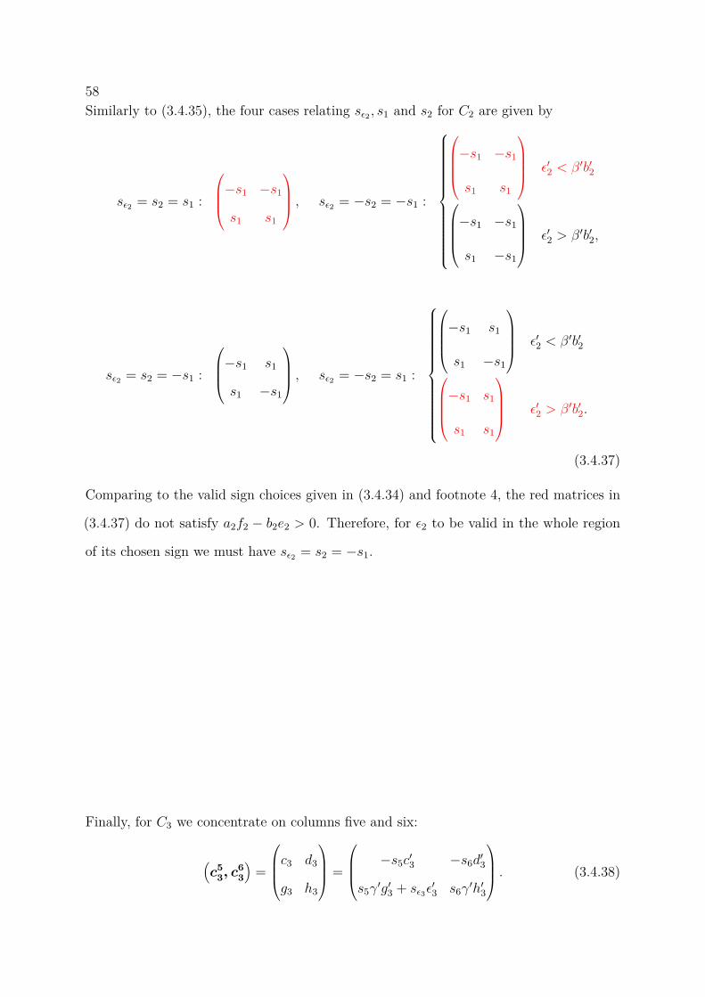
58Similarly to (3.4.35), the four cases relating sε2 , s1 and s2 for C2 are given by

sε2 = s2 = s1 :

−s1 −s1

s1 s1

, sε2 = −s2 = −s1 :

−s1 −s1

s1 s1

ε′2 < β′b′2

−s1 −s1

s1 −s1

ε′2 > β′b′2,

sε2 = s2 = −s1 :

−s1 s1

s1 −s1

, sε2 = −s2 = s1 :

−s1 s1

s1 −s1

ε′2 < β′b′2

−s1 s1

s1 s1

ε′2 > β′b′2.

(3.4.37)

Comparing to the valid sign choices given in (3.4.34) and footnote 4, the red matrices in

(3.4.37) do not satisfy a2f2 − b2e2 > 0. Therefore, for ε2 to be valid in the whole region

of its chosen sign we must have sε2 = s2 = −s1.

Finally, for C3 we concentrate on columns five and six:

(c5

3, c63

)=

c3 d3

g3 h3

=

−s5c′3 −s6d

′3

s5γ′g′3 + sε3ε

′3 s6γ

′h′3

. (3.4.38)

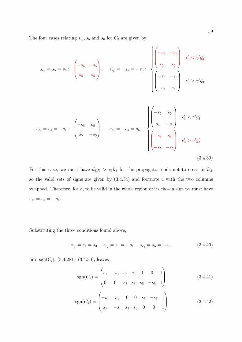
59The four cases relating sε3 , s5 and s6 for C3 are given by

sε3 = s5 = s6 :

−s5 −s5

s5 s5

, sε3 = −s5 = −s6 :

−s5 −s5

s5 s5

ε′3 < γ′g′3

−s5 −s5

−s5 s5

ε′3 > γ′g′3,

sε3 = s5 = −s6 :

−s5 s5

s5 −s5

, sε3 = −s5 = s6 :

−s5 s5

s5 −s5

ε′3 < γ′g′3

−s5 s5

−s5 −s5

ε′3 > γ′g′3.

(3.4.39)

For this case, we must have d3g3 > c3h3 for the propagator ends not to cross in D3,

so the valid sets of signs are given by (3.4.34) and footnote 4 with the two columns

swapped. Therefore, for ε3 to be valid in the whole region of its chosen sign we must have

sε3 = s5 = −s6.

Substituting the three conditions found above,

sε1 = s4 = s3, sε2 = s2 = −s1, sε3 = s5 = −s6, (3.4.40)

into sgn(Ci), (3.4.28) - (3.4.30), leaves

sgn(C1) =

s1 −s1 s3 s3 0 0 1

0 0 s3 s3 s5 −s5 1

(3.4.41)

sgn(C2) =

−s1 s1 0 0 s5 −s5 1

s1 −s1 s3 s3 0 0 1

(3.4.42)

60

sgn(C3) =

s1 −s1 0 0 −s5 s5 1

0 0 s3 s3 s5 −s5 1

. (3.4.43)

These matrices give sets of signs for Ci relating to the WLDs in Figure 3.7 that are

consistent with the matching of the spurious boundary associated to case 1 of the three-

way cancellation, while ensuring that the propagators do not cross each other. These

signs are valid not only on the boundary, but also away from it.

Now, we look to see if the sign choices for D1,D2,D3 are consistent with the consecutive

matching of the other type of spurious boundary occurring when propagator ends approach

vertices. We will see that the set of signs is in fact not consistent; the problem comes down

to the difference in signs in the top row of (3.4.42) to those in the top row of (3.4.43).

Consider starting with diagram D2 in Figure 3.8 and moving the propagator defined

by the second line in C2 around the Wilson loop clockwise until it reaches a diagram

equivalent to D3. We match spurious boundaries in a similar way to section 3.3.2; at

each vertex, the whole matrix of signs in the relevant limit must match. The signs of the

top row, corresponding to the propagator left fixed, must remain the same. Under this

sequence of moves we get

sgn(C2)→

−s1 s1 0 0 s5 −s5 1

0 0 s′3 s′4 s′5 s′6 1

, (3.4.44)

where the primed variables here represent new signs not yet fixed in the process. 5

Comparing this new matrix to sgn(C3), (3.4.43), one can see immediately that the signs

on the top row are different regardless of what the primed signs in the bottom row become.

Therefore, the signs found from the matching of the three-way spurious boundary are not

consistent with the mathcing of the boundaries obtained by following the propagators

round the Wilson loop polygon. The WLDs cannot be glued together to form a geometry

without spurious boundaries with this choice of α, β and γ.

5In fact, we do also require s′3 = s3 and s′4 = s3 by the pairwise matching of consecutive spuriousboundaries. However, this is not necessary for the continuation of the argument.

61Case 2: α, β, γ > 0

We now consider the second possibility for having pairwise matching boundaries, illus-

trated on the right hand side of Figure 3.9, with α, β, γ > 0. Looking at the Figure, C1

and C ′2 should overlap when 1 < α < ∞ and 0 < β < 1 and C1 and C ′3 should overlap

when 0 < α < 1 and 0 < γ < 1. Now there is an additional overlap between C ′2 and C ′3when 1 < β <∞ and 1 < γ <∞.

At these overlaps, the entries of the rotated matrices (3.4.22-3.4.24) must be equal.

Defining the signs of the C1 variables as previously, (3.4.25), this means the signs of the

entries of C ′2 and C ′3, must be the same as those of C1 in the region where they overlap

with C1 (i.e. 0 < β < 1, 0 < γ < 1). However when β, γ > 1 some of the entries changes

sign due their dependence on β or γ. Thus the signs of the entries of the rotated C

matrices are as follows:

sgn(C1) :

s1 s2 s3 s4 0 0 1

0 0 s3 s4 s5 s6 1

0<α<∞

(3.4.45)

sgn(C ′2) :

s1 s2 s3 s4 0 0 1

0 0 s3 s4 s5 s6 1

0<β<1

,

s1 s2 s3 s4 0 0 1

0 0 −s3 −s4 −s5 −s6 1

1<β<∞(3.4.46)

sgn(C ′3) :

s1 s2 s3 s4 0 0 1

0 0 s3 s4 s5 s6 1

0<γ<1

,

−s1 −s2 −s3 −s4 0 0 1

0 0 s3 s4 s5 s6 1

1<γ<∞

.

(3.4.47)

Now, even before rotating C ′2 and C ′3 back, there is a clear problem. Looking at the

matrices in 3.4.46 and 3.4.47 for 1 < β <∞ and 1 < γ <∞, the matrices do not overlap

as they should. Matching diagram D2 with D1 correctly and D3 with D1 correctly fixes

the signs of the respective C matrices in a way that is incompatible with D2 and D3

matching.

Therefore, there is no valid three way boundary matching for this case.

623.5 Concluding Remarks

We have shown that it is not possible to consistently assign a subspace of Gr(k, k + 4),

amplituhedron space, to each WLD consistent with its canonical form and pairwise

matching of all spurious boundaries. Therefore, WLDs cannot be used to tessellate

the amplituhedron, or in fact any other subspace, without spurious boundaries. This

is somewhat surprising since they do have certain properties which seem promising:

WLDs do have a natural, though non-unique, interpretation as subspaces in Gr(k, k + 4)

and they do sum to give the amplitude. The situation is similar to the toy example

shown in Figure 3.1 where region I and II clearly have canonical forms which sum to

give the quadrilateral with no spurious poles, but there are spurious boundaries left

unmatched in the corresponding geometrical interpretation. For the simple example of

the quadrilateral we could of course choose a more sensible set of signs to give a tessellation

of the quadrilateral with no spurious boundaries left, but we have shown that for the

N2MHV WLDs and beyond this is not possible.

Despite only showing this for the N2 MHV case, it is quite clear that the proof holds for

higher helicity. One simply needs to add the extra propagators away from the three way

cancellation and recycle the same argument as given here. As stated before, showing this

for six points was only to easily illustrate some examples - the argument clearly holds for

any number of particles. Furthermore, although we have focussed only on tree level here,

it would be very surprising if the situation improved when moving to loop level.

One might hope that although the WLDs do not tessellate the amplituhedron that they

may instead give a nice tessellation of the squared amplituhedron [75, 88] which has a

more direct definition and for which there are 2k copies of most diagrams. However,

having attempted to make this consistent it does not seem to be the case.

Although the WLDs cannot provide a tessellation of the amplituhedron, they do still give

a very concrete and suggestive “tessellation” at the level of the canonical form. It seems

likely that this property generalises for more positive Grassmannians, and may prove

63useful in their further mathematical study. Despite not giving a “good geometrical region”

it may still be interesting to further understand the WLDs geometrically; studies in this

direction have begun, see for example [102,103].

Chapter 4

Single Particle Operators in N = 4

Super Yang-Mills

4.1 Introduction

The AdS/CFT correspondence, originally conjectured by Maldacena, describes a remark-

able relationship between two sets of theories; on one side are the theories of quantum

gravity formulated in terms of string theory, and on the other side are a type of quantum

theory known as conformal field theories [1–3]. Perhaps the most noted successful con-

firmation of the correspondence is the relationship between the half-BPS sector of N = 4

SYM in four dimensions and IIB string theory on AdS5 × S5. String states in the latter

theory are related to gauge invariant operators in the former and AdS amplitudes are

related to correlators of gauge invariant operators. Half-BPS operators are particularly

interesting as their quantum numbers are not renormalised, and certain (extremal) cor-

relators are protected from renormalisation. Therefore, they can be computed in the free

theory then taken trivially to strong coupling. These correlation functions at large N can

then be compared to a gravitational equivalent via the AdS/CFT correspondence (see for

example [104–107]).

The correspondence has been used to reconstruct information on strong ’t Hooft coupling

66phenomena in gauge theory from semiclassical physics in AdS. For example, the operators

dual to single particle operators, which will be the main focus of this chapter, are expected

to vanish as the charge of the operator exceeds the number of colours N . From the

gravity side, as the angular momentum of a particle moving on the S5 increases, the

point-like graviton expands into a D3-brane wrapping an S3 ⊂ S5, [108] which cannot

grow bigger than the size of the S5. This is the basis of the stringy exclusion principle

(originally proposed in [109], see for example [110, 111] for further discussion). More

recently, the correspondence has been used successfully in the other direction; analytic

bootstrap techniques on the CFT side at strong coupling have allowed for more concrete

investigations of perturbative quantum gravity. For example, one-loop quantum gravity

amplitudes in AdS have been obtained by computing O(

1N4

)corrections to strong coupling

correlators in SYM [112–116].

In order for these investigations to be precise, and to properly account for the operator

product expansion (OPE) at tree level and one loop, it was necessary for the gauge

theory operators dual to single-particle supergravity states to be defined carefully. These

operators are half-BPS operators, therefore are protected. However, due to the degenerate

nature of the space of half-BPS operators, only in the planar limit can single particle

operators be identified as the well known single-trace operators Tr (φp), where p is the

charge (these will be introduced in more detail below). The single trace operators were

already known to receive O(

1N

)corrections from multi-trace operators [117–119]; in

fact, the first order double trace corrections have recently been worked out directly

from supergravity [120, 121]. However, the non-perturbative natrue of the AdS/CFT

correspondence heavily indicates that a non-perturbative definition should exist for the

states dual to single particles, i.e. one which remains valid for all N . Such a definition

was formulated in [122]:

Single-particle operators are half-BPS operators which have vanishing two-point

functions with all multi-trace operators.

(4.1.1)

67Up to normalisation, the above definition fixes the single particle operators uniquely as a

sum of the single trace operator and multi-trace operators with pre-factors dependent on

N . This definition of the operator has already been necessary for correctly determining

the one-loop O(

1N4

)supergravity correlators of operators with charges higher than four.

For example, arbitrary charge correlators in position space were studied in [115] and

〈22pp〉 correlators were calculated in Mellin space in [116].

The purpose of this chapter is to explore the properties of the single particle operators

defined above, find explicit formulae for them and calculate various correlation functions

involving them. We will begin by introducing the trace basis, as well as some properties

of half-BPS operators in N = 4 SYM. We will then proceed to introduce two more bases

of half-BPS operators, the dual basis and the schur polynomial basis, both of which we

will refer to when writing an explicit formula for our single-particle operators. This will

act as a brief review of concepts required to understand the rest of the chapter, and allow

us to set up notation.

4.1.1 Half-BPS Operators in N = 4 SYM and the Trace Basis

Here, we will very briefly review some properties of half-BPS operators in N = 4 SYM.

For a more thorough description see [4] and the references therein.

The half-BPS operators are built from the 6 real scalars, Xi, in the Yang-Mills theory

which lie in the (0, l, 0) representations of the SU(4) ∼ SO(6) R-symmetry group. These

are the symmetric traceless representations of SO(6) that correspond to Young diagrams

with one row of length l. They include single trace operators, where the trace is taken over

the gauge indices of a tensor product of the real scalars, and products of these forming

multi-trace operators. The 12 -BPS stress-tensor supermultiplet contains the protected

half-BPS operators Tr(φ2), the stress tensor and the (on-shell) chiral Lagrangian of the

theory.

In order to make sense of these operators, it is useful to introduce the SO(6) ∼ SU(4)

68null auxiliary variables YR, where null enforces Y · Y = 0 and R = 1, . . . , 6. The R-index

coincides with the SO(6) R-symmetry index. The single trace operators are then defined

as follows;

Tp(x) = Trφ(x)p ; φ(X, Y ) = Y RφR(X), (4.1.2)

where the variables Y R have been used to project the elementary field φR onto the

symmetric traceless representation. Therefore, a single insertion point xi corresponds not

only to a space-time coordinate Xi, but also an SO(6) vector Y R.

In this chapter, the U(N) theory will be particularly useful due to its simplicity, however

the bulk AdS theory is describing the SU(N) part of the theory.1 When working with

the SU(N) gauge group, we will denote the scalar field as ψ(x) ≡ ψ(X, Y ) = Y RψR(X),

where now the Y R are traceless.

To compute correlation functions in free field theory we use elementary propagators. The

conformal structure of the theory dictates that the two point function of two scalar fields

is given by

〈φa(x)φb(y)〉 = gab

(x− y)2 , (4.1.3)

where the indices a, b run over the adjoint representation of the gauge group and gab is

the inverse of gab = Tr(Y aY b

), the bilinear invariant. For the rest of the chapter we

will only be interested in the group structure of the correlator, therefore we will drop the

spacetime dependence. Taking the gauge group to be U(N) or SU(N), the propagator

takes the form

〈φsr(X1, Y1)φut (X2, Y2)〉 = δur δst g12 U(N) (4.1.4)

〈ψsr(X1, Y1)ψut (X2, Y2)〉 =(δur δ

st −

1Nδsrδ

ut

)g12 SU(N), (4.1.5)

1A U(N) gauge theory is equivalent to a free U(1) vector multiplet times an SU(N) gauge theory upto ZN identifications. It was shown in [123] that the U(1) part of the gauge group is a singleton fieldrelated to the centre of mass motion of the branes (the interested reader is encouraged to see [124] andthe references therein.

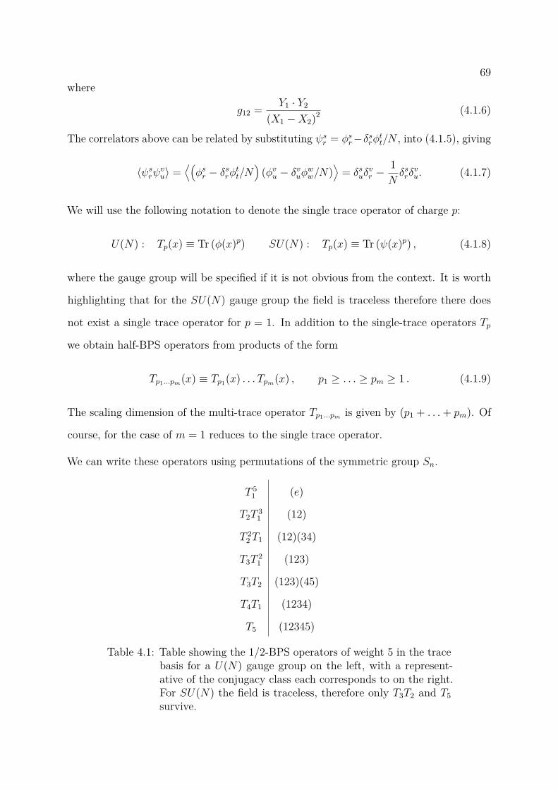
69where

g12 = Y1 · Y2

(X1 −X2)2 (4.1.6)

The correlators above can be related by substituting ψsr = φsr−δsrφtt/N , into (4.1.5), giving

〈ψsrψvu〉 =⟨(φsr − δsrφtt/N

)(φvu − δvuφww/N)

⟩= δsuδ

vr −

1Nδsrδ

vu. (4.1.7)

We will use the following notation to denote the single trace operator of charge p:

U(N) : Tp(x) ≡ Tr (φ(x)p) SU(N) : Tp(x) ≡ Tr (ψ(x)p) , (4.1.8)

where the gauge group will be specified if it is not obvious from the context. It is worth

highlighting that for the SU(N) gauge group the field is traceless therefore there does

not exist a single trace operator for p = 1. In addition to the single-trace operators Tp

we obtain half-BPS operators from products of the form

Tp1...pm(x) ≡ Tp1(x) . . . Tpm(x) , p1 ≥ . . . ≥ pm ≥ 1 . (4.1.9)

The scaling dimension of the multi-trace operator Tp1...pm is given by (p1 + . . .+ pm). Of

course, for the case of m = 1 reduces to the single trace operator.

We can write these operators using permutations of the symmetric group Sn.

T 51 (e)

T2T31 (12)

T 22 T1 (12)(34)

T3T21 (123)

T3T2 (123)(45)

T4T1 (1234)

T5 (12345)

Table 4.1: Table showing the 1/2-BPS operators of weight 5 in the tracebasis for a U(N) gauge group on the left, with a represent-ative of the conjugacy class each corresponds to on the right.For SU(N) the field is traceless, therefore only T3T2 and T5survive.

70Taking the set of weight five operators as an example and letting σ ∈ S5, with p1, . . . , pm

denoting the lengths of the cycles of σ (∑mi=1 pi = 5),we write

Tr (σφ(x)) ≡ Tp1,...,pm(x) ≡ φi1iσ(1)φi2iσ(2)

φi3iσ(3)φi4iσ(4)

φi5iσ(5). (4.1.10)

For example, if σ = (12)(345) we get the operator

φi1i2φi2i1φ

i3i4φ

i4i5φ

i5i3 = T3T2 (4.1.11)

One can see that the trace structure is only dependent on the cycle structure of the

permutations; for example, the permutation (12)(345) gives the same trace structure as

(14)(235). Therefore, the multi-trace operators in the U(N) gauge theory are in one-to-one

correspondence with the conjugacy classes of the permutation group Sn. Table 4.1 shows

the correspondence between multi-trace operators of weight 5 and the conjugacy classes

of S5.

Since the fields ψ are traceless, the correspondence for the SU(N) gauge theory is between

multi-trace operators and conjugacy classes of Sn with no cycles of length 1, e.g. for

the weight 5 example above there is an operator corresponding to the conjugacy class

with elements (12)(345) and (12345) (see Table 4.1). Letting p(n) denote the number of

conjugacy classes of Sn, the number of conjugacy classes that do not contain a 1-cycle is

p(n)− p(n− 1), since each element with a 1-cycle can be decomposed into a 1-cycle and

an element of Sn−1.

We refer to the basis of half-BPS operators made of all possible Tp1...pm(x) as the trace

basis, and for the remainder of the chapter will denote the basis elements with the symbol

Tp, where p stands for a partition of p. A correlation function of operators in the trace

basis will have the schematic form

〈Tp1(x1) . . . Tpn(xn)〉 =∑bij

∏i,j

gbijij Cbij, p1...pn(N), (4.1.12)

where bij counts the number of propagators from insertion point i to j, and biji<j is the

collection of these bridges labelling the propagator structure. The corresponding colour

71factor is given by Cbij, p1...pn(N).

4.1.2 Other Bases of Half-BPS Operators

Other than the trace basis, there are two other bases of the half-BPS operators that

will be useful to be familiar with; the schur basis and the dual basis. Here we give the

definition of these two bases, we state group theoretic formulae for them and illustrate

some of their basic properties.

Schur Basis

A beautiful orthogonal basis for all half-BPS operators in the U(N) theory was given

in [125] in terms of Schur polynomials, where by orthogonal we mean the operators

diagonalise the two point function.

The Schur polynomial basis is defined as a sum of the trace basis operators discussed in

section 4.1.1 over the elements σp1...pm ∈ Sp, weighted by the characters of σp1...pm in the

representation R of Sp

χR(φ) = 1n!

∑σ∈Sp

χR(σ) Tr (σφ) . (4.1.13)

As mentioned in section 2.4.3, the representations R of Sp can be labelled by Young

diagrams with p boxes. Therefore, the operators in the Schur polynomial basis can also

be represented by these Young diagrams. Therefore, the number of Schur polynomials of

weight p is equal to the number of partitions of p. The representation R also corresponds

to a representation of U(N).2 For a unitary matrix U , the character of U in representation

R is given by χR(U) defined by (4.1.13).

The correlation function of two Schur polynomials calculated in [125] is given by

⟨χR(φ†)χS(φ)

⟩= δRSfR, (4.1.14)

2This is a consequence of the fact that if V is the fundamental representation of U(N), U(N) and Sn

have a commuting action on V⊗

n. For more details see for example [72].

72where fR is defined in (2.4.14). Finally, we can invert the relation between the Schur

polynomials and trace basis operators. Multiplying (4.1.13) by χR(τ) and summing over

the representations R we have

∑R

χR(τ)χR (φ) = 1p!∑σ∈Sp

∑R

χR(σ)χR(τ) Tr(σφ)

=∑σ∈Sp

1p!

p!|[σ]|δ ([τ ] = [σ]) Tr(σφ)

= Tr(τφ), (4.1.15)

where to get to the second line we have used the orthogonality relation (2.4.9). The

third line follows from the observation that the only terms in the sum over elements that

survive from line two are those that have σ in the same conjugacy class as τ , of which

there are |[τ ]| terms.

The Schur polynomials have some very nice properties, including that they automatically

truncate with N , since a U(N) Young diagram with height larger than N vanishes. One

can see this very easily by noticing the dimension of the representation R of U(N),

(2.4.12), will be zero if the number of boxes in the first column surpasses N . Therefore,

this set of operators automatically satisfies one of the properties expected as a result of

the AdS/CFT correspondence. However, the basis does not project onto an orthogonal

basis for SU(N); indeed, the operators are not even linearly independent in the SU(N)

theory.

Dual Basis

In [126] a non-orthogonal but linearly independent basis of all SU(N) half-BPS operators

was defined. This basis was later identified as the dual to the trace basis in [127] via the

metric defined by the two point function, and a group theoretic expression for this basis

was given:

ξp1...pn(x) = |[σp1...pn ]|p!

∑R`p

1fRχR(σp1...pn)χR(φ) p1 ≥ . . . ≥ pn, (4.1.16)

73where |[σp1...pn ]| is the size of the conjugacy class given labelled by the cycle lengths p1 . . . pn

(see (2.4.4)), the sum is over the representations of Sp labelled by Young diagrams with

p boxes and weighted by fR defined in (2.4.14). Here, χR(σp1...pn) is the character of

σp1...pn in R and χR(φ) is the Schur polynomial discussed in the previous section. These

are operators ξp1...pn (with p1 ≥ . . . ≥ pn) which obey

〈ξp1...pm(x1)Tq1...qn(x2)〉 =

1 if (p1, . . . , pm) = (q1, . . . , qn) ,

0 otherwise.(4.1.17)

In other words each element of the dual to the trace basis is orthogonal to (i.e. it has

vanishing two-point function with) all elements of the trace basis but one, and we then

normalise it to have unit two-point coefficient with this element. This can be seen

straightforwardly by substituting (4.1.15) and (4.1.16) into the two-point function:

〈ξp1...pm(x1)Tq1...qn(x2)〉 = |[σp1...pn ]|p!

∑R`p

1fRχR(σp1...pn)

∑S`p

χS(σq1...qn)〈χR(φ†)χS(φ)〉

= |[σp1...pn ]|p!

∑R`p

χR(σp1...pn)χR(σq1...qn)

= δp1q1 . . . δpmqn , (4.1.18)

where the second line uses the diagonal nature of the Schur basis (4.1.14) and the third

line uses the orthogonality relation (2.4.8). The delta functions in the final line simply

impose that the elements of Sn being considered must be in the same conjugacy class.

We will refer to the basis given by the ξp1,...,pn as the dual basis.

By definition, the change of basis matrix from the dual to the trace basis is simply the

two point function:

ξp1...pn(x) =∑

q1...qm`p〈ξp1...pnξq1...qm〉Tq1...qm(x) (4.1.19)

where the sum is over all partitions of p, that is all sets of integers q1 ≥ · · · ≥ qm such

that q1 + ... + qm = p. Using (4.1.16) with (4.1.14), one finds the two-point function of

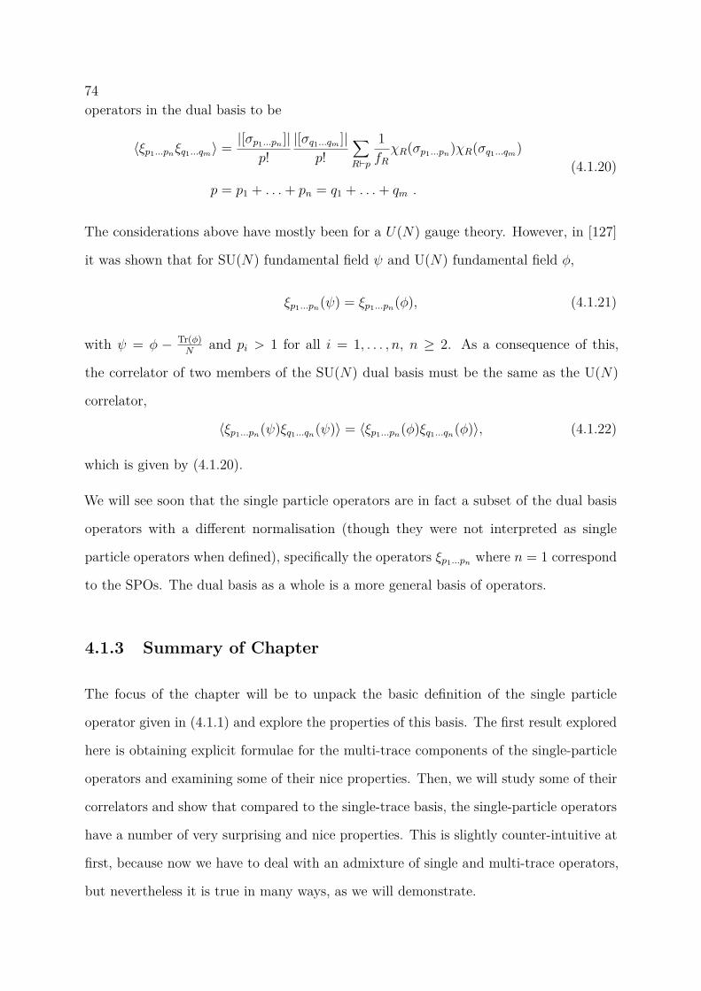
74operators in the dual basis to be

〈ξp1...pnξq1...qm〉 = |[σp1...pn ]|p!

|[σq1...qm ]|p!

∑R`p

1fRχR(σp1...pn)χR(σq1...qm)

p = p1 + . . .+ pn = q1 + . . .+ qm .

(4.1.20)

The considerations above have mostly been for a U(N) gauge theory. However, in [127]

it was shown that for SU(N) fundamental field ψ and U(N) fundamental field φ,

ξp1...pn(ψ) = ξp1...pn(φ), (4.1.21)

with ψ = φ − Tr(φ)N

and pi > 1 for all i = 1, . . . , n, n ≥ 2. As a consequence of this,

the correlator of two members of the SU(N) dual basis must be the same as the U(N)

correlator,

〈ξp1...pn(ψ)ξq1...qn(ψ)〉 = 〈ξp1...pn(φ)ξq1...qn(φ)〉, (4.1.22)

which is given by (4.1.20).

We will see soon that the single particle operators are in fact a subset of the dual basis

operators with a different normalisation (though they were not interpreted as single

particle operators when defined), specifically the operators ξp1...pn where n = 1 correspond

to the SPOs. The dual basis as a whole is a more general basis of operators.

4.1.3 Summary of Chapter

The focus of the chapter will be to unpack the basic definition of the single particle

operator given in (4.1.1) and explore the properties of this basis. The first result explored

here is obtaining explicit formulae for the multi-trace components of the single-particle

operators and examining some of their nice properties. Then, we will study some of their

correlators and show that compared to the single-trace basis, the single-particle operators

have a number of very surprising and nice properties. This is slightly counter-intuitive at

first, because now we have to deal with an admixture of single and multi-trace operators,

but nevertheless it is true in many ways, as we will demonstrate.

75One of the nice properties of SPOs is the operators in the U(N) theory and the SU(N)

theory are very closely related. In fact, writing the SPOs in terms of the trace basis,

the operators in the SU(N) theory are found simply by setting all T1 to zero. Since

the elementary field, ψ, in SU(N) is the traceless part of the elementary field, φ, in

U(N), Indeed, in the U(N) theory the single-particle operators of charge greater than

or equal to two must be orthogonal to all multi-trace operators involving any Tr(φ), and

this automatically makes them the SU(N) operators. To formalise this statement we

introduce the SU(N) projection on the space of the U(N) operators, and show that the

U(N) single-particle operators belong to the SU(N) subspace, which is orthogonal to

the span of multi-trace operators in which at least one trace is Tr(φ). It follows that

correlators of U(N) single-particle operators are equal to correlators of SU(N) single-

particle operators.

Another nice property of the single-particle operators is that they automatically vanish if

the charge of the operators exceeds the number of colours N . This should be contrasted

for example with the single trace basis which does not vanish, but rather decomposes

into complicated linear combinations of products of lower trace operators. In [128], (sub)-

determinant half-BPS operators were defined as duals to these sphere giants (discussed

briefly in the introduction) and later these particles were associated with the completely

antisymmetric (single column Young diagram) Schur polynomials [125]. At large N we

find that the single-particle operators with charge close to N do indeed approach these

(sub)-determinant operators.

The rest of the chapter will be organised as follows:

• In section 4.2 we discuss the details of the multi-trace admixture which defines the

single-particle operators. We first give explicit examples at low charge, and then we

use group theory techniques to obtain a general formula, valid for any single-particle

operator of any charge p. Our formulae allow us to study the ‘shape’ of the operator

in the large N limit, and in particular to see explicitly the interpolation between

76the single-trace and the sphere giant as a function of p (see section 4.2.3). Moreover,

we will be able to compute the two-point function normalisation exactly.

• In section 4.3 we uplift the defining two-point function orthogonality to a multi-point

orthogonality theorem, which in turn implies vanishing of a large class of diagrams

in correlators. We call these near-extremal n-point functions, where extremality will

be defined as a measure of how much the diagram is connected w.r.t. the heaviest

operator (see (4.3.11)). This is the first instance of hidden simplicity of multi-point

single-particle correlators versus the single-trace correlators, and very interestingly,

a similar feature was noticed on the (super-)gravity side in [129].

• In section 4.4, we consider the first non vanishing correlators, and we study maximally-

extremal (ME) and next-to-maximally extremal (NME) n-point functions. Both are

simple. The ME correlators are computed by trees and two point functions. The

NME are mostly computed by weighted sums of ME correlators, which we know in

general. When we compute these correlators by using Wick contractions techniques

on the trace basis, the combinatorics is hard in the intermediate steps. Instead, the

final result is way much simpler. We provide more evidence about this mechanism

mentioning also the case of NNME three-point functions.

Most of the work here is based off of published work in [58]. I contributed at least in

part to all sections being presented in this thesis. Section 5 as well as most of Appendix

B and all of C from the paper are not present in this thesis as that was the work of my

collaborators; I had no part in it.

4.2 Single-Particle Half-BPS Operators (SPOs)

The simple definition of the SPOs given in [122] was the following:

Single-particle operators are half-BPS operators which have vanishing two-point

77

functions with all multi-trace operators.

In this section we will make this definition more precise, find explicit formulae for the

operators in terms of the trace basis, the eigenvalues of the operators and the Schur

polynomials, and provide some examples in each of the three bases. We then show two

important properties of the SPOs; one, SPOs interpolate between single-trace and giant

gravitons, and two, that the operators are the same in U(N) as SU(N). Finally, we

show the explicit formula for their two-point functions, and make some comments on the

possibility of extending from single-particle operators to an orthogonal basis of multi-

particle operators. For the most part we shall ignore the space-time dependence, since it

is the colour factor we are most interested in; the space-time dependence can usually be

reconstructed straightforwardly after the fact.

4.2.1 Definition of SPOs and Low Charge Examples

The AdS/CFT correspondence maps the spectrum of operators in N = 4 super Yang-Mills

theory to the spectrum of IIB superstring theory on the AdS5 × S5 background. The

superstring can be found in unexcited states (giving the IIB supergravity multiplet) or

excited states. The half-BPS operators correspond to the supergravity states and their

multi-particle products.

In the natural basis of scattering states, the multi-particle states should be orthogonal to

single-particle ones. A key observation, though, for the purposes of the discussion here is

that the trace basis of half-BPS operators is not an orthogonal basis with repect to the

inner product given by the two-point functions. In general,

〈Tp(x1)Tq1...qn(x2)〉 6= 0 n ≥ 2 . (4.2.1)

In order to align with the AdS/CFT intuition, a prescription was given in [115,122] for

identifying the relevant half-BPS operators Op that correspond to single particle states.

The definition simply states that the operators are those which are orthogonal to all

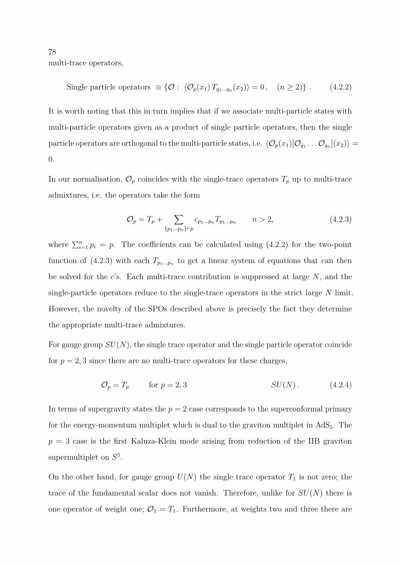
78multi-trace operators,

Single particle operators ≡ O : 〈Op(x1)Tq1...qn(x2)〉 = 0 , (n ≥ 2) . (4.2.2)

It is worth noting that this in turn implies that if we associate multi-particle states with

multi-particle operators given as a product of single particle operators, then the single

particle operators are orthogonal to the multi-particle states, i.e. 〈Op(x1)[Oq1 . . .Oqn ](x2)〉 =

0.

In our normalisation, Op coincides with the single-trace operators Tp up to multi-trace

admixtures, i.e. the operators take the form

Op = Tp +∑

p1...pn`pcp1...pnTp1...pn n > 2, (4.2.3)

where ∑ni=1 pi = p. The coefficients can be calculated using (4.2.2) for the two-point

function of (4.2.3) with each Tp1...pn to get a linear system of equations that can then

be solved for the c’s. Each multi-trace contribution is suppressed at large N , and the

single-particle operators reduce to the single-trace operators in the strict large N limit.

However, the novelty of the SPOs described above is precisely the fact they determine

the appropriate multi-trace admixtures.

For gauge group SU(N), the single trace operator and the single particle operator coincide

for p = 2, 3 since there are no multi-trace operators for these charges,

Op = Tp for p = 2, 3 SU(N) . (4.2.4)

In terms of supergravity states the p = 2 case corresponds to the superconformal primary

for the energy-momentum multiplet which is dual to the graviton multiplet in AdS5. The

p = 3 case is the first Kaluza-Klein mode arising from reduction of the IIB graviton

supermultiplet on S5.

On the other hand, for gauge group U(N) the single trace operator T1 is not zero; the

trace of the fundamental scalar does not vanish. Therefore, unlike for SU(N) there is

one operator of weight one; O1 = T1. Furthermore, at weights two and three there are

79multi-trace operators that involve T1, specifically T11 for weight two and T21, T111 for

weight three, for which our single particle particle operator is defined to be orthogonal

to. Therefore, they have multi-trace contributions:

O2 = T2 − 1NT11

O3 = T3 − 3NT21 + 2

N2T111

U(N) . (4.2.5)

The additional terms compared to the SU(N) operators (4.2.4) simply project out the

trace part of the fundamental scalar φ and so the SU(N) and U(N) operators in fact

coincide.

For p > 3, we have the first non-trivial admixtures in SU(N) as well as U(N), which can

be verified using the propagator (4.1.5). This was discussed in [122], with some previous

discussion in [117, 119, 130]. For example, the single particle operator for p = 4 is given

by

O4 = T4 −2N2 − 3N(N2 + 1)T22 SU(N) , (4.2.6)

where the coefficient of the double-trace contribution determined from the orthogonality

condition 〈O4T22〉 = 0.3 In the U(N) theory, the SPO with p = 4 has further contributions

involving T1. It is given by

O4 = T4 −(2N2 − 3)N (N2 + 1)T22 + 10

N2 + 1T211 −4NT13 −

5N (N2 + 1)T1111 U(N) , (4.2.7)

where the coeffcients are determined by demanding orthogonality with all higher trace

operators T22, T211, T13 and T1111.

We see that the SU(N) operators can be found from the U(N) operators by imposing

T1 = 0. This pattern continues for p > 4; we give the next couple of cases to illustrate

this,

O5 = T5 −5 (N2 − 2)T32

N (N2 + 5) + U5, (4.2.8)

3Other attempts at finding this combination can be found in [131].

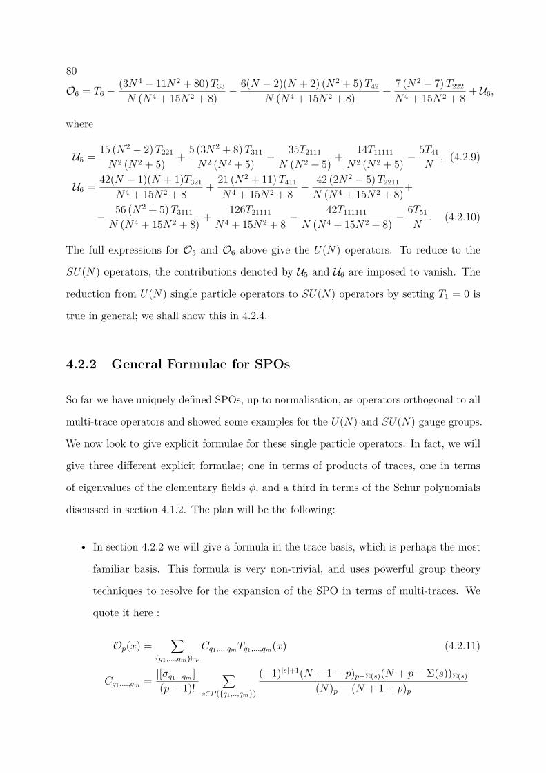
80

O6 = T6 −(3N4 − 11N2 + 80)T33

N (N4 + 15N2 + 8) − 6(N − 2)(N + 2) (N2 + 5)T42

N (N4 + 15N2 + 8) + 7 (N2 − 7)T222

N4 + 15N2 + 8 + U6,

where

U5 = 15 (N2 − 2)T221

N2 (N2 + 5) + 5 (3N2 + 8)T311

N2 (N2 + 5) − 35T2111

N (N2 + 5) + 14T11111

N2 (N2 + 5) −5T41

N, (4.2.9)

U6 = 42(N − 1)(N + 1)T321

N4 + 15N2 + 8 + 21 (N2 + 11)T411

N4 + 15N2 + 8 −42 (2N2 − 5)T2211

N (N4 + 15N2 + 8)+

− 56 (N2 + 5)T3111

N (N4 + 15N2 + 8) + 126T21111

N4 + 15N2 + 8 −42T111111

N (N4 + 15N2 + 8) −6T51

N. (4.2.10)

The full expressions for O5 and O6 above give the U(N) operators. To reduce to the

SU(N) operators, the contributions denoted by U5 and U6 are imposed to vanish. The

reduction from U(N) single particle operators to SU(N) operators by setting T1 = 0 is

true in general; we shall show this in 4.2.4.

4.2.2 General Formulae for SPOs

So far we have uniquely defined SPOs, up to normalisation, as operators orthogonal to all

multi-trace operators and showed some examples for the U(N) and SU(N) gauge groups.

We now look to give explicit formulae for these single particle operators. In fact, we will

give three different explicit formulae; one in terms of products of traces, one in terms

of eigenvalues of the elementary fields φ, and a third in terms of the Schur polynomials

discussed in section 4.1.2. The plan will be the following:

• In section 4.2.2 we will give a formula in the trace basis, which is perhaps the most

familiar basis. This formula is very non-trivial, and uses powerful group theory

techniques to resolve for the expansion of the SPO in terms of multi-traces. We

quote it here :

Op(x) =∑

q1,...,qm`pCq1,...,qmTq1,...,qm(x) (4.2.11)

Cq1,...,qm = |[σq1...qm ]|(p− 1)!

∑s∈P(q1,..,qm)

(−1)|s|+1(N + 1− p)p−Σ(s)(N + p− Σ(s))Σ(s)

(N)p − (N + 1− p)p

81The group theory data consists of P(q1, . . . , qm), the powerset of the traces Tq1,...,qm ,

then |s| is the cardinality of s and Σ(s) = ∑si∈s si (see section 2.4.6). Finally,

|[σq1...qm ]| is the size of the conjugacy classes of σ with length cycles q1 . . . qm, given

by (2.4.4).

• In section 4.2.2 we give a much simpler formula, directly in terms of the eigenvalues

Ek(zi) of the elementary fields φ,

Op(x) =p∑

k=1dk(p,N)Ek(zi)(x) (4.2.12)

dk(p,N) = (−1)k+1p (N − p+ 1)p−k(p− 1)k(N)p − (N − p+ 1)p

• Finally, in section 4.2.2 we give another simple formula in terms of the Schur

polynomials introduced in section 4.1.2:

Op =p∑

k=1dk(p,N)χRp

k[φ], (4.2.13)

dk(p,N) = p(p−1)(−1)k−1 (N−k+p+1)k−1(N−p+1)p−k(N)p − (N−p+1)p,

where we note that only Schur polynomials of hook representations appear.

If we consider half-BPS operators to be symmetric functions of the eigenvalues of the

scalar matrix φsr, we see the three bases introduced above all correspond to well known

bases for symmetric polynomials:

Trace basis←→ Power sum symmetric polynomials

Eigenvalue monomials←→ Monomial symmetric polynomials

Schur polynomial operators←→ Schur polynomials,

where the second correspondence is true after eigenvalue monomials are summed over per-

mutations. There are a number of well known formulae relating three bases of symmetric

polynomials on the right hand side known as Newton identities. It would be interesting

82to explore these relations in the context of the bases of single particle operators on the

left hand side.

Formula in terms of a product of traces

In section 4.1.2 we described a linearly independent basis of half-BPS operators known as

the dual basis, and gave group theoretic formulae for them and their two point functions

introduced by Brown in [127]. They were operators defined to be orthogonal to all

elements of the trace basis bar one; see (4.1.17). The dual field ξp of the single trace

operator Tp satisfies

〈ξp(x1)Tq1...qn(x2)〉 = 0 , n ≥ 2. (4.2.14)

In fact, this corresponds precisely to our single particle operators, Op (see (4.2.2)), there-

fore the single particle operators must be equal to the dual field ξp up to normalisation.

Since Op = Tp+ multi-traces, (4.2.14) and 〈ξpTp〉 = 1 we find

〈ξpOp〉 = 1, (4.2.15)

hence

ξp(x) = Op(x)〈OpOp〉

and Op(x) = ξp(x)〈ξpξp〉

. (4.2.16)

We look to use the change of basis matrix from the dual to the trace basis given in

(4.1.19) for ξp to find an explicit formula for the multi-trace admixtures for the single

particle operator. We need the two-point function of two dual basis elements given in

(4.1.20) for ξp1...pn = ξp. The conjugacy class corresponding to the single index dual

basis operator consists of a cycle of length p, of which there are (p − 1)! possibilities

meaning |[σp]| = (p−1)!. Furthermore, for this conjugacy class we observe that only hook

representations have a non-vanishing character. More specifically,

χR(σp) =

(−1)hR−1 R = hook YT of height hR

0 otherwise,(4.2.17)

83where by “hook YT” we mean that the representations R that are associated to hook-

shaped diagrams: Young diagrams that only have boxes in the first row and first column.

Substituting this information into (4.1.20) gives

〈ξp ξq1..qm〉 = 1p

|[σq1..qm ]|p!

∑R∈ hooks

1fR

(−1)1+hRχR(σq1..qm) , (4.2.18)

which are the coefficients of the multi-trace operators in ξp. In all of the many cases we

have explored, we have observed that this sum over hook representations is given by the

following explicit formula:

〈ξp ξq1..qm〉 = 1p

|[σq1..qm ]|p!

1p− 1

∑s∈P(q1,..,qm)

(−1)|s|+1

(N + 1− Σ(s))p−1, (4.2.19)

where the notation corresponds to the group theoretic tools introduced in section 2.4.6.

An important special case of (4.2.19) is the case m = 1 giving the two-point function of

the dual of the single trace operator. In this case the sum is over just two elements since

P(p) = , p. The expression (4.2.19) thus simplifies to

〈ξp ξp〉 = 1p2

1p− 1

(1

(N+1−p)p−1− 1

(N+1)p−1

). (4.2.20)

Finally, inserting (4.1.19), (4.2.19) and (4.2.20) into Op(x) = ξp(x)〈ξpξp〉 gives an explicit

expression for the single particle operator as a sum of multi-trace operators

Op(x) =∑

q1..qm`pCq1,..,qmTq1,..qm(x) (4.2.21)

with coefficients

Cq1,..qm = 〈ξp ξq1..qm〉〈ξp ξp〉

= |[σq1..qm ]|(p− 1)!

∑s∈P(q1,..,qm)

(−1)|s|+1

(N + 1− Σ(s))p−1

(1

(N + 1− p)p−1− 1

(N + 1)p−1

)−1

= |[σq1..qm ]|(p− 1)!

∑s∈P(q1,..,qm)

(−1)|s|+1(N + 1− p)p−Σ(s)(N + p− Σ(s))Σ(s)

(N)p − (N + 1− p)p, (4.2.22)

where the size of the conjugacy class is given by (2.4.4). The second equality is more

useful computationally and is obtained by multiplying and dividing by (N + 1− p)2p−1

84and using the identity

(N + 1− p)2p−1

(N + 1− Σ(s))p−1= (N + 1− p)p−Σ(s)(N + p− Σ(s))Σ(s) . (4.2.23)

Therefore, we have arrived at an explicit formula for computing the coefficients Cq1...qm ,

allowing us to write the single particle operator of any p in the trace basis. Very nicely,

this formula is explicit in p and q1, . . . , qm and depends only on the group theory data

associated to such a partition.4

The value of m splits the single particle operator into different trace sectors. In Appendix

B we provide some examples for generic q1 . . . qm when m = 2 and m = 3, i.e. the

double trace and triple trace sectors respectively.

Formula in terms of eigenvalues

The single single particle operator can in fact be written in a much simpler way when

expressed directly in terms of the eigenvalues of the adjoint scalar φsr, which we will label

z1, z2, . . . , zN . Before we write down the explicit formula we introduce the monomial

symmetric polynomials, mλ(z1 . . . zN):

mλ(z1, . . . , zN) =∑

σ′∈SNzλσ′(1)1 z

λσ′(2)2 . . . z

λσ′(N)N , (4.2.24)

4This is unlike the formula given by Brown for the dual basis, (4.1.16), which requires the input ofadditional information, namely the value of the character χR(σq1...qm

). A coefficient in (4.2.21) can becalculated by only knowing the partition of p corresponding to the trace structure of the multi-traceoperator the coefficient in question multiplies.

85where the λ is short hand for (λ1, . . . , λN) with λ1 ≥ λ2 ≥ . . . ≥ λN , and the sum is over

all distinct permutations of (λ1, λ2, . . . , λN). Some examples of these polynomials include:

m(1,1,1) (z1, z2, z3) = z1z2z3,

m(3,2,0) (z1, z2, z3) = z31z

22 + z3

1z23 + z3

2z21 + z3

2z23 + z3

3z21 + z3

3z22 ,

m(3,1,0,0) (z1, z2, z3, z4) = z31z2 + z3

1z3 + z31z4 + z3

2z1 + z32z3 + z3

2z4 + z33z1 + z3

3z2 + z33z4

+ z34z1 + z3

4z2 + z34z3.

(4.2.25)

It will be useful to introduce the sum over all monomials indexed by a partition of p in k

parts, which we label Ep,k:

Ep,k(z1, . . . zN) =∑

q1+...+qk=pq1≥q2≥...qk>0

m[q1,...,qk,0N−k](z1, . . . zN). (4.2.26)

The most obvious example of (4.2.26) is Ep,1(z1, . . . , zN) = zp1 + . . . + zpN = Tp. Some

other examples include

Ep,p(z1 . . . zN) = z1 . . . zp + . . .

E4,2(z1 . . . zN) = (z31z2 + . . .) + (z2

1z22 + . . .)

(4.2.27)

We find that the single-particle operators can be written as 5

Op =p∑

k=1dk(p,N)Ep,k(zi) , (4.2.28)

where the coefficient dk(p,N) is

dk(p,N) = (−1)k+1p (N − p+ 1)p−k(p− 1)k(N)p − (N − p+ 1)p

= (−1)k (p− 1)k(N − k + 1)k

p

1− (N)p(N−p+1)p

(4.2.29)

Note that interestingly the coefficient of a monomial in this formula only depends on the

number of different eigenvalues appearing in the monomial and not on any other details

5More precisely, in all of the many cases we explored, we always find that this formula is valid.

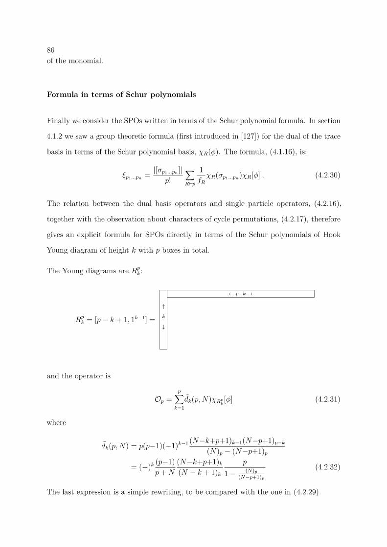
86of the monomial.

Formula in terms of Schur polynomials

Finally we consider the SPOs written in terms of the Schur polynomial formula. In section

4.1.2 we saw a group theoretic formula (first introduced in [127]) for the dual of the trace

basis in terms of the Schur polynomial basis, χR(φ). The formula, (4.1.16), is:

ξp1...pn = |[σp1...pn ]|p!

∑R`p

1fRχR(σp1...pn)χR[φ] . (4.2.30)

The relation between the dual basis operators and single particle operators, (4.2.16),

together with the observation about characters of cycle permutations, (4.2.17), therefore

gives an explicit formula for SPOs directly in terms of the Schur polynomials of Hook

Young diagram of height k with p boxes in total.

The Young diagrams are Rpk:

Rpk = [p− k + 1, 1k−1] =

← p−k →

↑

k

↓

and the operator is

Op =p∑

k=1dk(p,N)χRp

k[φ] (4.2.31)

where

dk(p,N) = p(p−1)(−1)k−1 (N−k+p+1)k−1(N−p+1)p−k(N)p − (N−p+1)p

= (−)k (p−1)p+N

(N−k+p+1)k(N − k + 1)k

p

1− (N)p(N−p+1)p

(4.2.32)

The last expression is a simple rewriting, to be compared with the one in (4.2.29).

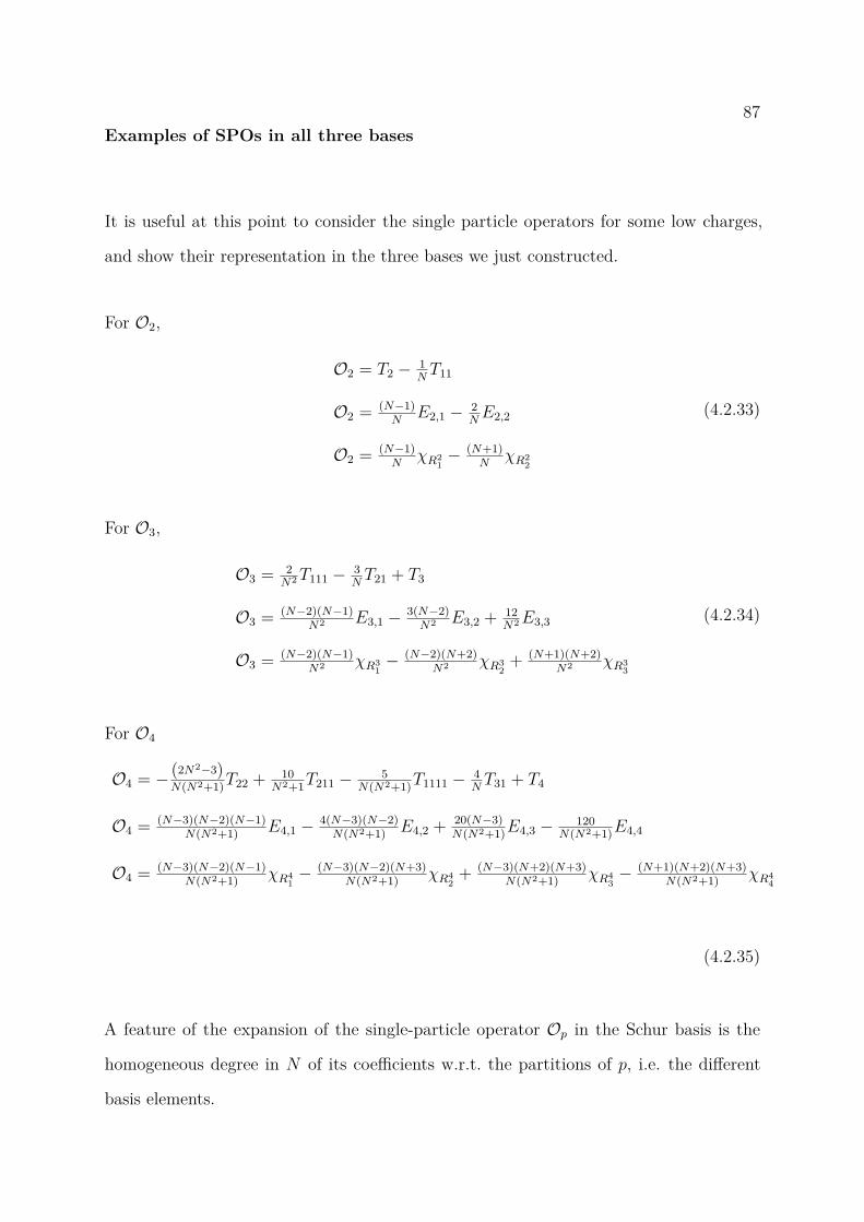
87Examples of SPOs in all three bases

It is useful at this point to consider the single particle operators for some low charges,

and show their representation in the three bases we just constructed.

For O2,

O2 = T2 − 1NT11

O2 = (N−1)N

E2,1 − 2NE2,2

O2 = (N−1)N

χR21− (N+1)

NχR2

2

(4.2.33)

For O3,

O3 = 2N2T111 − 3

NT21 + T3

O3 = (N−2)(N−1)N2 E3,1 − 3(N−2)

N2 E3,2 + 12N2E3,3

O3 = (N−2)(N−1)N2 χR3

1− (N−2)(N+2)

N2 χR32

+ (N+1)(N+2)N2 χR3

3

(4.2.34)

For O4

O4 = − (2N2−3)N(N2+1)T22 + 10

N2+1T211 − 5N(N2+1)T1111 − 4

NT31 + T4

O4 = (N−3)(N−2)(N−1)N(N2+1) E4,1 − 4(N−3)(N−2)

N(N2+1) E4,2 + 20(N−3)N(N2+1)E4,3 − 120

N(N2+1)E4,4

O4 = (N−3)(N−2)(N−1)N(N2+1) χR4

1− (N−3)(N−2)(N+3)

N(N2+1) χR42

+ (N−3)(N+2)(N+3)N(N2+1) χR4

3− (N+1)(N+2)(N+3)

N(N2+1) χR44

(4.2.35)

A feature of the expansion of the single-particle operator Op in the Schur basis is the

homogeneous degree in N of its coefficients w.r.t. the partitions of p, i.e. the different

basis elements.

884.2.3 SPOs interpolate between single-trace operators and

giant gravitons

The single particle operators, which have a definition directly in N = 4 SYM, involve

protected operators and are thus non-perturbative. As was anticipated in the introduc-

tion, the definition was strongly motivated via the AdS/CFT correspondence on the

supergravity side by certain properties of KK modes on AdS5 × S5 [117–119]. In this

section, we shall investigate how the single particle operator behaves at large N as we

vary p. This has been well understood in the gravity dual [108,128], therefore we use this

analysis to provide some further evidence that our SPOs should be identified with the

single-particle half-BPS excitations of AdS5 × S5.

Recall that the regime of validity of the gravitational description of N = 4 SYM is

the regime in which N is the largest parameter. The correspondence of the single-trace

operators with the KK spectrum in the strict large N limit is a very well known fact.

We will now show that the single particle operators do in fact become the single-trace

operator in this limit.

The most direct way to see this is using the formula in terms of eigenvalues given by

(4.2.28) and (4.2.29). In this formula p is explicit and held fixed in the limit. Using the

Stirling approximation, namely n! ∼√

2πn(ne

)nfor n→∞, we find

dk(p,N)d1(p,N) →

(−)k−1

Nk−1Γ[p+ k − 1]

Γ[p] as N →∞. (4.2.36)

For k > 1 the contribution is suppressed. As described below (4.2.26), the terms with

k = 1 are precisely zp1 + . . . + zpN , i.e. the single trace term. Therefore, in the large N

limit we have

Op → Tp +O(1/N) (4.2.37)

as expected.6 The agreement of the multi-trace admixture in the 1/N expansion can be

6Though not as direct, one can see this from the formula for SPOs in the trace basis, (4.2.21)

89tested from supergravity computations in [117–119], and more generally is consistent with

the OPE (discussed in [115]).

In a slightly different line of consideration, drawing inspiration from the work of Myers

[132], giant gravitons were predicted on the gravity side when increasing charge p, [108].

The observation was that for increasing angular momentum, equal to the charge p, the

type-IIB graviton becomes less pointline on the sphere, and grows into a D3 brane

wrapping an S3 embedded in S5. However, the radius cannot grow to be greater than the

S5, which provided the constraint p/N ≤ 1. We will show now that the single particle

operator matches with the picture described above; it cuts off if p > N with both p,N

finite, and becomes a giant sphere graviton in the large N limit with p ∼ N . In particular,

we will see it matches with the operator proposed to be the dual of the spherical D3 brane

in [128].

Firstly, consider the charge p of the single-particle operator increasing such that eventually

it exceeds the number of colours N . As p > N , the single trace operators become linear

combinations of multi-trace operators. However, the single particle operators vanish:

Op = 0 ; p > N. (4.2.38)

This is very easy to see in the explicit examples given in (4.2.33), (4.2.34) and (4.2.35).

This can be explained from the original definition of SPOs; single particle operators are

by definition orthogonal to all multi-trace operators. For p > N there are only multi-trace

operators, therefore the single particle operators must be orthogonal to all operators and

so must vanish. This is one very evident way in which the behaviour of our single particle

operators is very different from the single trace operators.

Finally, we consider the behaviour of the single particle operators in the regime in which

p = N − p′ with p,N 1 and p′ ≥ 0 fixed. (4.2.39)

and (4.2.22), too. Each term in the sum of Cq1...qmis O(N), however the alternating sum provides a

cancellation at each order in N for a total of m cancellations. Therefore, we end up with O(1/Nm−1),

in agreement with the considerations of the large N limit in the eigenvalue basis.

90To do this, we shall consider the behaviour of coefficient dk(p,N) from the eigenvalue

basis in (4.2.29) normalised with respect to dp(p,N):

D ≡ dk(p,N)dp(p,N) = (−1)k−pΓ(−k + n+ 1)Γ(k + p− 1)

Γ(2p− 1)Γ(n− p+ 1) . (4.2.40)

Introducing the variable k′ ≡ p − k ≥ 0, the giant graviton regime is found when k′ is

small. Substituting this into (4.2.40) gives

D(k′) = (−1)−k′Γ[2p− 1− k′]Γ[1 + p′ + k′]Γ[2p− 1]Γ[1 + p′] ; k′ ≡ p− k ≥ 0. (4.2.41)

For small k′, D(k′) ∼ O(1/(2p)k′

), and since p ∼ N at leading order, the Ep,k coefficients

are power-law suppressed in the large N limit, apart from the coefficient of Ep,p which

becomes the dominant term. Therefore, we obtain 7

Op → (−)p+1p

(1

1 + pN

)N−p+1

Ep,p +O(1/N) ; p,N 1 and p−N fixed,

(4.2.42)

where the pre-factor comes from the limit of dp(p,N). Therefore, the single particle

operator becomes proportional to the sub-determinant operator Ep,p.

The sub-determinant operators were originally proposed in [128] to be duals to the D3

branes studied in [108]. We have seen above that the single particle operator becomes

precisely the sub-determinant operator in the limit (4.2.39). Furthermore, since the sub-

determinant operator corresponds to the totally antisymmetric Schur polynomial, the

giant graviton limit localises the single particle operator onto the single column Schur

polynomial, as is expected from [125].

4.2.4 SPOs in U(N) are SPOs in SU(N)

As we saw for the low charge examples in (4.2.5), (4.2.7) and (4.2.8), the single particle

operators in the U(N) and SU(N) gauge groups are very closely related. In particular,

7For values of k′ → N we probe the contribution of other Ep,k in the sum (4.2.28), since k → 1. Inthis limit D(k′) ∼

√πN1/2+p′

e−2N log 2, therefore their contribution is exponentially suppressed, and wecan localise the sum on Ep,p.

91despite the elementary fields of the two theories, being different in general, the U(N)

SPOs represented in the trace basis give the SPOs in the SU(N) theory simply be setting

T1 to zero. This suggests that SPOs in U(N) are SPOs in SU(N); here we look to make

this statement more rigorous.

Let φsr and ψsr label the fields of the U(N) and SU(N) theories respectively. The field ψsris the traceless part of the field φsr,

ψrs = φr

s − 1Nδsrφt

t . (4.2.43)

For any operator O[φ] in U(N) we define the SU(N) projection as the map,

Π : O[φ] → O[φ] ≡ O[ψ(φ)] (4.2.44)

The operator O[φ] is then a new operator in U(N). As an example, we show how the

SU(N) projection map works for the operator O[φ] = Tr(φ2):

O[φ] = ψsr(φ)ψrs(φ)

=(φsr −

1Nδsrφ

uu

)(φrs −

1Nδrsφ

vv

)= φsrφ

rs −

1Nφsrδ

rsφ

vv −

1Nφrsδ

srφ

uu + 1

N2 δsrφ

uuδrsφ

vv

= Tr(φ2)︸ ︷︷ ︸O[φ]

− 1N

Tr(φ) Tr(φ). (4.2.45)

More generally we find that an operator projected using the map (4.2.44) takes the form

O[φ] = O[φ]− [T1O[φ]] ; T1 = Tr[φ] (4.2.46)

for some operator O[φ]. Notice that in treating φ and ψ as formal variables, O[φ] is the

leading term in the 1N

expansion of O[φ].

Since the field ψ is traceless, the projection of any U(N) operator made of products of

traces that has T1 in the product will be 0, with all other projections giving something

non-zero of the form (4.2.46). Therefore, the map Π : O → O decomposes the space of

U(N) operators into Im(Π)⊕Ker(Π), where all operators in the kernel are of the form

92[T1O[φ]].

We now look to calculate the two-point function of an operator O[φ] with an operator in

the kernel of the projection, specifically

〈O(x1) [T1O](x2)〉U(N) . (4.2.47)

The operator O[φ] is constructed from only the traceless part of φsr. By applying Wick’s

theorem to compute (4.2.47), there will always be a contraction between one of the fields

in O(x1) and T1(x2). Using the U(N) theory propagator given by (4.1.4) on this particular

contraction we get

〈ψsr(x1)T1(x2)〉 = 〈φsr(x1)φtt(x2)〉 − 1Nδsr〈φuu(x1)φtt(x2)〉

= δsr −1NδsrN

= 0.

(4.2.48)

Therefore, any operator O[φ] constructed from only the traceless part of the field φ is

orthogonal to any operator involving the trace as a factor, [T1O].

Single particle operators in U(N) were defined to be orthogonal to all multi-trace operators,

meaning they must be orthogonal to operators of the form [T1O]. Therefore, single particle

operators in U(N) automatically live in the SU(N) subspace. It is now possible that

SU(N) single particle operators give the U(N) single particle operators. The only thing

that remains to be checked is the U(N) inner product restricted on the SU(N) subspace

is the same as the inner product of the SU(N) theory. To do this we calculate the two

point function of two elements of ψ(φ) using the U(N) propagator

〈ψsr(φ)ψut (φ)〉U(N) =⟨(φsr − 1

Nδsrφ

vv

)(φut − 1

Nδut φ

vv

)⟩U(N)

= δur δst − 1

Nδsrδ

ut . (4.2.49)

This gives precisely the SU(N) propagator defined in (4.1.5).

Therefore, we conclude that U(N) single-particle operators are SPOs in SU(N)

OU(N)p [φ] = OSU(N)

p [ψ] p ≥ 2 (4.2.50)

93and any correlators of SPOs of charge 2 or higher computed in either U(N) or SU(N)

will be identical. This result manifests the well known feature of the free part of N = 4

SYM in the context of AdS/CFT, that the U(1) part of the gauge group U(N) decouples

and only the SU(N) remains in the interacting theory.

4.2.5 Two-point Function Properties

From the discussion of single particle operators in the trace basis (see section 4.1.1), we

found that the normalisation of the two-point function of single particle operators is given

by the inverse of the two-point function of dual basis elements. Letting Rp denote the

N -dependent colour factor we have

〈Op(x1)Op(x2)〉 = Rp gp12 ; 〈ξp(x1)ξp(x2)〉 = 1

Rp

gp12 (4.2.51)

where we saw from (4.2.20) that Rp takes the form

Rp = p2(p− 1)[

1(N − p+ 1)p−1

− 1(N + 1)p−1

]−1

. (4.2.52)

The single particle operators vanish when N < p, therefore we would expect Rp to have

zeros at N = 1, . . . , p − 1. Furthermore, since it is symmetric in N → −N it would be

expected that it contains explicit factors of (N2 − r2) for r = 1, . . . , p − 1, rather than

just (N − r). This property of Rp can be made manifest by writing it in the form

Rp = p

Qp(N)

p−1∏r=1

(N2 − r2) , (4.2.53)

where Qp(N) is a polynomial of degree (p− 2) in N . The first few cases of Qp are given

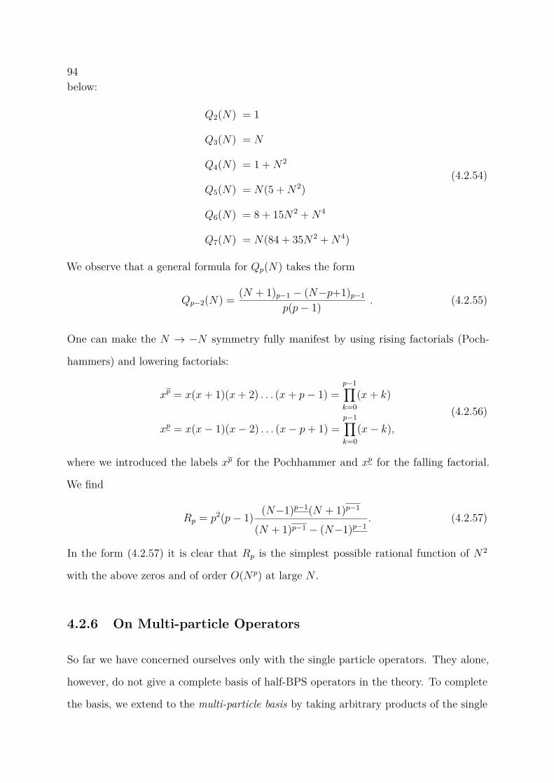
94below:

Q2(N) = 1

Q3(N) = N

Q4(N) = 1 +N2

Q5(N) = N(5 +N2)

Q6(N) = 8 + 15N2 +N4

Q7(N) = N(84 + 35N2 +N4)

(4.2.54)

We observe that a general formula for Qp(N) takes the form

Qp−2(N) = (N + 1)p−1 − (N−p+1)p−1

p(p− 1) . (4.2.55)

One can make the N → −N symmetry fully manifest by using rising factorials (Poch-

hammers) and lowering factorials:

xp = x(x+ 1)(x+ 2) . . . (x+ p− 1) =p−1∏k=0

(x+ k)

xp = x(x− 1)(x− 2) . . . (x− p+ 1) =p−1∏k=0

(x− k),(4.2.56)

where we introduced the labels xp for the Pochhammer and xp for the falling factorial.

We find

Rp = p2(p− 1) (N−1)p−1(N + 1)p−1

(N + 1)p−1 − (N−1)p−1. (4.2.57)

In the form (4.2.57) it is clear that Rp is the simplest possible rational function of N2

with the above zeros and of order O(Np) at large N .

4.2.6 On Multi-particle Operators

So far we have concerned ourselves only with the single particle operators. They alone,

however, do not give a complete basis of half-BPS operators in the theory. To complete

the basis, we extend to the multi-particle basis by taking arbitrary products of the single

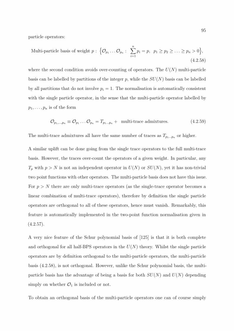
95particle operators:

Multi-particle basis of weight p :Op1 . . .Opn :

n∑i=1

pi = p, p1 ≥ p2 ≥ . . . ≥ pn > 0,

(4.2.58)

where the second condition avoids over-counting of operators. The U(N) multi-particle

basis can be labelled by partitions of the integer p, while the SU(N) basis can be labelled

by all partitions that do not involve pi = 1. The normalisation is automatically consistent

with the single particle operator, in the sense that the multi-particle operator labelled by

p1, . . . , pn is of the form

Op1,...,pn ≡ Op1 . . .Opn = Tp1...pn + multi-trace admixtures. (4.2.59)

The multi-trace admixtures all have the same number of traces as Tp1...pn or higher.

A similar uplift can be done going from the single trace operators to the full multi-trace

basis. However, the traces over-count the operators of a given weight. In particular, any

Tp with p > N is not an independent operator in U(N) or SU(N), yet it has non-trivial

two point functions with other operators. The multi-particle basis does not have this issue.

For p > N there are only multi-trace operators (as the single-trace operator becomes a

linear combination of multi-trace operators), therefore by definition the single particle

operators are orthogonal to all of these operators, hence must vanish. Remarkably, this

feature is automatically implemented in the two-point function normalisation given in

(4.2.57).

A very nice feature of the Schur polynomial basis of [125] is that it is both complete

and orthogonal for all half-BPS operators in the U(N) theory. Whilst the single particle

operators are by definition orthogonal to the multi-particle operators, the multi-particle

basis (4.2.58), is not orthogonal. However, unlike the Schur polynomial basis, the multi-

particle basis has the advantage of being a basis for both SU(N) and U(N) depending

simply on whether O1 is included or not.

To obtain an orthogonal basis of the multi-particle operators one can of course simply

96implement the Gram Schmidt procedure. The idea is as follows: start with an ordered

list of basis elements, leave the first element unchanged, and run over the rest in order

by adding linear combinations of all previously considered elements such that the new

element is orthogonal to all previous ones. As an example, for the charge six operators

the trace basis operators could be ordered in the following way

(T111111, T21111, T2211, T3111, T222, T321, T411, T33, T42, T51, T6) U(N)

(T222, T33, T42, T6) SU(N). (4.2.60)

Performing Gram-Schmidt orthogonalisation (with respect to either the U(N) or SU(N)

two-point function) in the order from left to right would provide an orthogonal set of

operators. Assuming the single-particle operator should be found as part of this procedure,

it makes sense to have T6 last in the ordering as this corresponds directly to the definition

of the SPO. However, it is not clear if there is a canonical choice for the ordering of the

other operators. Inspired by the SPO, it would be very natural to define two-particle

operators as those which are orthogonal to triple traces and higher. This would give

a natural ordering of trace basis elements from highest number of traces to the lowest.

However, doing so still leaves ambiguity within each trace sector; even at weight six, the

double trace sector has three operators T33, T42, T51 in the U(N) theory and two T33, T4,2

in the SU(N) theory, and it is unclear if there is a canonical choice.

Assuming the single-particles are fixed so provide a starting point for organising an order-

ing, a completely equivalent way of obtaining the same orthogonal basis is to start with

the dual basis, list the operators in reverse order, and perform Gram-Schmidt orthogonal-

isation. This process yields exactly the same orthogonal basis up to normalisation. Using

the weight six operators to illustrate this as above,

(ξ6, ξ51, ξ42, ξ33, ξ411, ξ321, ξ222, ξ3111, ξ2211, ξ21111, ξ111111) U(N)

(ξ6, ξ42, ξ33, ξ222) SU(N) (4.2.61)

In the first approach the operator with the most traces T111111 (or T222) remains unchanged

97whereas the single-particle operator is the most complicated from the point of view of the

trace-basis. In the second approach, the opposite is true; the single particle operator is

ξp, and an operator labelled by a partition with increasing length becomes more intricate

from the point of view of the ξ basis. In the end, the most intricate of such operators, a

linear combination of all dual operators, must equal T11111 (or T222).

We leave the task of extending the single-particle operators to a full orthogonal basis to a

future work. Perhaps an AdS/CFT understanding of multi-particle KK modes will help

us figuring out a canonical way to fix the multi-particle states in N = 4 SYM.

4.3 Multipoint Orthogonality

In the previous section we obtained explicit expressions for the SPOs. Given that the

single particle operator is constructed from all single- and multi-trace operators, one

would expect such a rich structure would lead to very complicated multipoint correlation

functions. In particular, one would assume that they are much more complicated than

multipoint single-trace correlation functions. However, this expectation turns out to be

too naive. In this section, we look to describe one unexpected simplification of multipoint

correlation functions; we will prove that the defining two-point function orthogonality

uplifts to a multipoint orthogonality theorem. This in turn implies that a large class of

diagrams vanishes.

Multipoint Orthogonality Theorem. Consider any diagram contributing to a half-

BPS correlator that has a single particle operator Op connected to two sub-diagrams,

with the sub-diagrams themselves disconnected from each other. Any propagator structure

consistent with this type of diagram has a vanishing colour factor. This statement holds

for both U(N) and SU(N) free theories.

We will consider n operators; one will be a weight p single particle operator Op, r operators

labelled by q1, . . . , qr will form one sub-diagram and the remaining operators labelled by

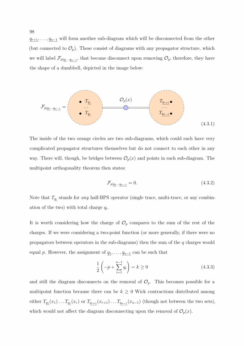
98qr+1, . . . , qn−1 will form another sub-diagram which will be disconnected from the other

(but connected to Op). These consist of diagrams with any propagator structure, which

we will label Fp|q1...qn−1 , that become disconnect upon removing Op; therefore, they have

the shape of a dumbbell, depicted in the image below:

Op(x)

Tqn−1

. . .

Tqr+1

Tqr

. . .

Tq1

Fp|q1...qn−1 =

(4.3.1)

The inside of the two orange circles are two sub-diagrams, which could each have very

complicated propagator structures themselves but do not connect to each other in any

way. There will, though, be bridges between Op(x) and points in each sub-diagram. The

multipoint orthogonality theorem then states:

Fp|q1...qn−1 = 0. (4.3.2)

Note that Tqi stands for any half-BPS operator (single trace, multi-trace, or any combin-

ation of the two) with total charge qi.

It is worth considering how the charge of Op compares to the sum of the rest of the

charges. If we were considering a two-point function (or more generally, if there were no

propagators between operators in the sub-diagrams) then the sum of the q charges would

equal p. However, the assignment of q1, . . . , qn−1 can be such that

12

(−p+

n−1∑i=1

qi

)= k ≥ 0 (4.3.3)

and still the diagram disconnects on the removal of Op. This becomes possible for a

multipoint function because there can be k ≥ 0 Wick contractions distributed among

either Tq1(x1) . . . Tqr(xr) or Tqr+1(xr+1) . . . Tqn−1(xn−1) (though not between the two sets),

which would not affect the diagram disconnecting upon the removal of Op(x).

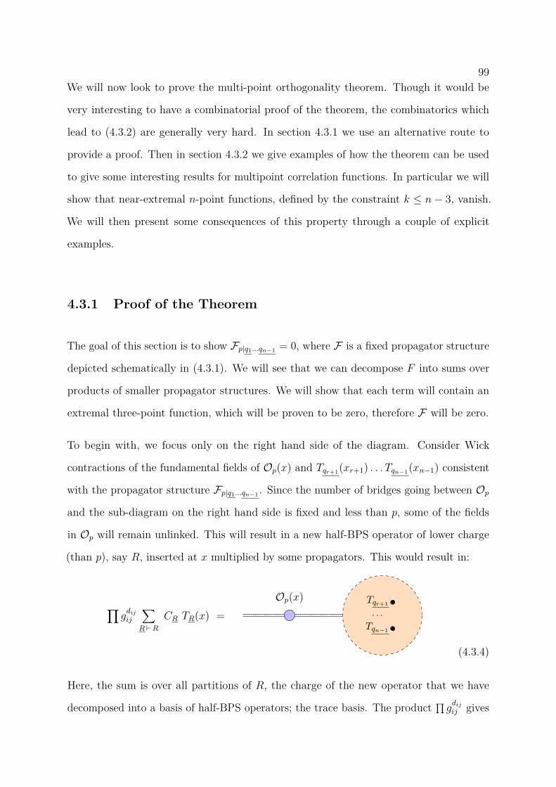
99We will now look to prove the multi-point orthogonality theorem. Though it would be

very interesting to have a combinatorial proof of the theorem, the combinatorics which

lead to (4.3.2) are generally very hard. In section 4.3.1 we use an alternative route to

provide a proof. Then in section 4.3.2 we give examples of how the theorem can be used

to give some interesting results for multipoint correlation functions. In particular we will

show that near-extremal n-point functions, defined by the constraint k ≤ n− 3, vanish.

We will then present some consequences of this property through a couple of explicit

examples.

4.3.1 Proof of the Theorem

The goal of this section is to show Fp|q1...qn−1 = 0, where F is a fixed propagator structure

depicted schematically in (4.3.1). We will see that we can decompose F into sums over

products of smaller propagator structures. We will show that each term will contain an

extremal three-point function, which will be proven to be zero, therefore F will be zero.

To begin with, we focus only on the right hand side of the diagram. Consider Wick

contractions of the fundamental fields of Op(x) and Tqr+1(xr+1) . . . Tqn−1(xn−1) consistent

with the propagator structure Fp|q1...qn−1 . Since the number of bridges going between Op

and the sub-diagram on the right hand side is fixed and less than p, some of the fields

in Op will remain unlinked. This will result in a new half-BPS operator of lower charge

(than p), say R, inserted at x multiplied by some propagators. This would result in:

∏gdijij

∑R`R

CR TR(x) =Op(x)

Tqn−1

. . .

Tqr+1

(4.3.4)

Here, the sum is over all partitions of R, the charge of the new operator that we have

decomposed into a basis of half-BPS operators; the trace basis. The product ∏ gdijij gives

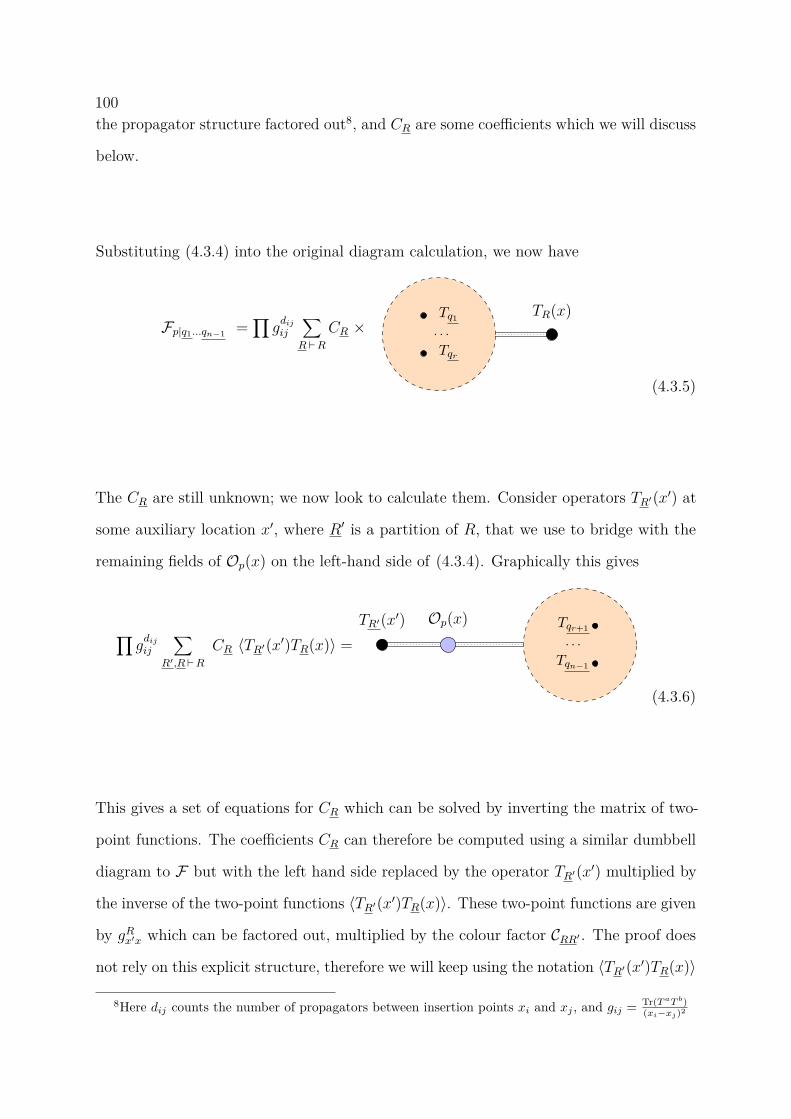
100the propagator structure factored out8, and CR are some coefficients which we will discuss

below.

Substituting (4.3.4) into the original diagram calculation, we now have

TR(x)

Tqr

. . .

Tq1Fp|q1...qn−1 =

∏gdijij

∑R`R

CR ×

(4.3.5)

The CR are still unknown; we now look to calculate them. Consider operators TR′(x′) at

some auxiliary location x′, where R′ is a partition of R, that we use to bridge with the

remaining fields of Op(x) on the left-hand side of (4.3.4). Graphically this gives

∏gdijij

∑R′,R`R

CR 〈TR′(x′)TR(x)〉 =Op(x)

Tqn−1

. . .

Tqr+1TR′(x′)

(4.3.6)

This gives a set of equations for CR which can be solved by inverting the matrix of two-

point functions. The coefficients CR can therefore be computed using a similar dumbbell

diagram to F but with the left hand side replaced by the operator TR′(x′) multiplied by

the inverse of the two-point functions 〈TR′(x′)TR(x)〉. These two-point functions are given

by gRx′x which can be factored out, multiplied by the colour factor CRR′ . The proof does

not rely on this explicit structure, therefore we will keep using the notation 〈TR′(x′)TR(x)〉

8Here dij counts the number of propagators between insertion points xi and xj , and gij = Tr(T aT b)(xi−xj)2

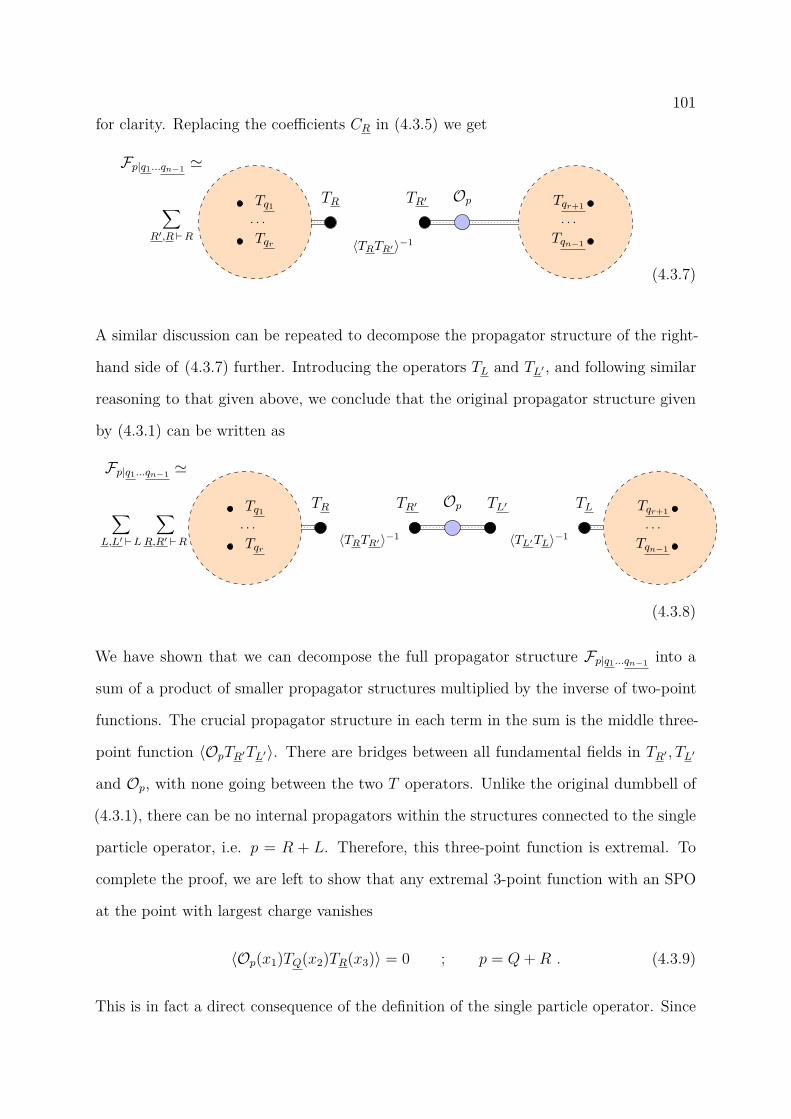
101for clarity. Replacing the coefficients CR in (4.3.5) we get

TR′

〈TRTR′〉−1

TR Op

Tqn−1

. . .

Tqr+1

Tqr

. . .

Tq1∑R′,R`R

Fp|q1...qn−1 '

(4.3.7)

A similar discussion can be repeated to decompose the propagator structure of the right-

hand side of (4.3.7) further. Introducing the operators TL and TL′ , and following similar

reasoning to that given above, we conclude that the original propagator structure given

by (4.3.1) can be written as

TL′

〈TL′TL〉−1

TLTR′

〈TRTR′〉−1

TR Op

Tqn−1

. . .

Tqr+1

Tqr

. . .

Tq1∑L,L′ `L

∑R,R′ `R

Fp|q1...qn−1 '

(4.3.8)

We have shown that we can decompose the full propagator structure Fp|q1...qn−1 into a

sum of a product of smaller propagator structures multiplied by the inverse of two-point

functions. The crucial propagator structure in each term in the sum is the middle three-

point function 〈OpTR′TL′〉. There are bridges between all fundamental fields in TR′ , TL′

and Op, with none going between the two T operators. Unlike the original dumbbell of

(4.3.1), there can be no internal propagators within the structures connected to the single

particle operator, i.e. p = R + L. Therefore, this three-point function is extremal. To

complete the proof, we are left to show that any extremal 3-point function with an SPO

at the point with largest charge vanishes

〈Op(x1)TQ(x2)TR(x3)〉 = 0 ; p = Q+R . (4.3.9)

This is in fact a direct consequence of the definition of the single particle operator. Since

102there are no propagators running between operator TQ and TR, the three point function

can be directly related to the corresponding two-point function obtained by bringing the

points 2 and 3 together. Therefore,

〈OpTQTR〉 =(g13

g12

)R〈Op[TQTR]〉 = 0 , (4.3.10)

where the final equality is reached by using the fact the single particle operator is defined

to be orthogonal to all multi-trace operators.

Therefore, we have shown that any propagator structure involving Op which becomes

disconnected on removing Op vanishes, thus concluding our proof of the multipoint

orthogonality theorem.

4.3.2 Vanishing Near-Extremal Correlators

The remainder of this chapter will mostly be dealing with the calculation of n−point

functions involving the single particle operators. Before we do so, it is useful to introduce

what we will refer to as the degree of extremality, given by k. Let p be the largest charge,

and q1, . . . , qn−1 be the other charges. The degree of extramilty is defined as

k = 12

(−p+

n−1∑i=1

qi

). (4.3.11)

This should be familiar from (4.3.3) of the last section.

The n-point correlator 〈OpTq1 . . . Tqn−1〉 is zero for k < 0 purely by considering the SU(4)

symmetry. Extremal (k = 0) and next-to-extremal (k = 1) correlators were shown to

all be non-renormalised in [107, 130, 133–135], and a nice diagrammatic interpretation

of the non-renormalisation for the simplest case of two-point functions was given in for

example [136, 137]. Related to this quantity, the concept of “near-extremal” correlators

was introduced in [129]. These are n-point correlators that satisfy the following condition

near extremal correlator: k ≤ n− 3 . (4.3.12)

103For n = 3, only the extremal correlators (k = 0) are considered near-extremal by this

definition. For n = 4 the extremal and next-to-extremal correlators are considered near-

extremal, and for n ≥ 5 the correlators that satisfy (4.3.12) go beyond even extremal and

next-to-extremal functions.

We make the following claim:

Near-Extremal Correlators Vanish. Any near-extremal SU(N) correlator in free

theory, where the largest charge operator is a single-particle operator, vanishes, i.e.

〈Op(x)Tq1(x1) . . . Tqn−1(xn−1)〉 = 0 k ≤ n− 3 . (4.3.13)

In the U(N) theory, a similar statement can be made but with the caveat that it is true

only for connected correlators.

As usual, Tqi stands for any half-BPS operator with total charge qi. We remark that any

refers to any single- or multi-trace operator or any combination of these. A corollary of

this is that any near-extremal correlator involving only SPOs vanishes.

〈Op(x)Oq1(x1) . . .Oqn−1(xn−1)〉 = 0 k ≤ n− 3 . (4.3.14)

To prove (4.3.13), we will argue that every diagram contributing to the near-extremal

correlator has a dumbbell shape, so the same propagator structure as in (4.3.1). This will

mean every diagram gives a zero contribution, therefore the correlators are equal to zero.

Proof. Let us begin by showing that there are not enough propagators between the Tqioperators to connect all of them together. The total charge of these operators is given by∑qi = 2k + p, meaning that there are 2k + p propagator ends connected to them. We

know that p of the ends must come from propagators bridging between Op and the Tqi ,

therefore there are a total of k propagators between the Tqi themselves (which accounts

for the 2k+ p− p = 2k remaining ends). The minimal case that would allow all Tqi to be

connected to each other is if they were connected in a chain with one propagator between

each; i.e. k = n− 2. However, from near-extremality we have k ≤ n− 3, therefore there

104are not enough bridges between these operators; we would need at least two more points.

This is true for both SU(N) and U(N).

Since the topology of Op(x)Tq1(x1) . . . Tqn−1(xn−1) is such that it is not possible to connect

all Tqi , a connected diagram would have to take the form of the dumbbell as in (4.3.1).

Therefore, all connected diagrams for these correlators are equal to zero by the multi-point

orthogonality theorem described in the previous section.

The only possible exceptional case could be when the diagram is made of two disconnected

pieces i.e. one of the ends of the dumbbells is on its own completely. This would evade the

vanishing property of the full dumbbell diagrams. For concreteness, let us say without loss

of generality that Tq1(x1) . . . Tq

r(xr) is disconnected from Op(x)Tq

r+1(x1) . . . Tq

n−1(xn−1),

for some value of r. We now look to investigate when the propagator structure can be

disconnected in such a way. The number of propagators between the fields of the disconnec-

ted piece of the diagram, i.e. between Tq1(x1) . . . Tq

r(xr), is given by 1

2 (∑ri=1 qi). For the

other part of the disconnected diagram, the number of bridges among the Tqr+1 , . . . , Tqn−1

which are not connecting with Op is

kR = 12

−p+n−1∑i=r+1

qi

. (4.3.15)

We assume that this part of the diagram remains connected upon the removal of Op,

otherwise it would have a propagator structure like in (4.3.1) which would automatically

give zero. For this to happen, the operators Tqi with i = r + 1, . . . , n− 1 would have to

all be connected to each other. The minimal way this could happen is they form a tree,

which would require kR ≥ n− r − 2 propagators.

From the near-extremality condition we have

k = 12

(−p+

n−1∑i=1

qi

)≤ n− 3. (4.3.16)

Substituting (4.3.15) into (4.3.16) we find

12

r∑i=1

qi ≤ n− 3− kR ≤ r − 1, (4.3.17)

105where the last inequality comes from using kR ≥ n− r − 2. Focussing on the first part of

the inequality and the last, for this to be satisfied then at least two of the qi must equal

one. For SU(N) this is not possible since there are no charge one operators, therefore

there are no disconnected diagrams of the form being considered here. For the U(N)

theory, however, this is a possibility.

We conclude that all SU(N) diagrams (and connected U(N) diagrams) contributing

to near extremal correlators have a dumbbell shape as in (4.3.1) and therefore equal

zero. Thus, we have proven the statement made above regarding vanishing near-extremal

correlators.

Further Corollaries

A useful corollary of the vanishing of near-extremal correlators occurs for lower point

correlators, say m-points, which are not near extremal but have a number of multi-trace

operators.,

〈Op(x)Tq1(x1) . . . Tqm−1(xm−1)〉 ; k = 12(−p+

∑qi) ≥ m− 3 . (4.3.18)

Say r of the operators are multi-trace operators. We can think of (4.3.18) as the limit

of an n ≥ m point correlator, with specific propagator structure such that there are

no propagators inside any of the multi-traces. The maximum value for n is achieved

by putting all parts of the multi-traces on fictitious points. If we let l(qi) measure the

number of parts of qi, then

m ≤ n = (m− r) +r∑i=1

l(qi) (4.3.19)

If k ≤ n − 3 then the original correlator, (4.3.18), vanishes as it can be thought of an

n-point near-extremal correlator.

As a simple example of the above corollary, consider the three-point function between Op,

106Tq1 and Tq2 ;

if ∃ i such that l(qi) ≥ 2 and k ≤ 1 ⇒ 〈Op(x)Tq1(x1)Tq2(x2)〉 = 0. (4.3.20)

The correlation function is zero because one can always think of the three-point function

as the limit of a near-extremal higher point function, which we have shown vanishes.

A further example is the following:

if ∃ i such that l(qi) ≥ 2 and k ≤ m− 2 ⇒ 〈Op(x)Tq1(x1) . . . Tqm−1(xm−1)〉 = 0

(4.3.21)

There are many more possibilities that arise from this corollary. In particular, in the

above examples we have only considered one of the multi-trace operators being split,

however multiple of the operators could be split if they have a multi-trace structure. We

do not make an exhaustive list here, but point out that a consistent way of determining

if a correlator falls into one of the vanishing near-extremal cases is to fully split the

multi-trace operators up to consider the full n-point function, calculate the extremality

k using (4.3.11), then see if it satisfies k ≤ n− 3. If this inequality is satisfied, then the

n-point correlation function is zero, which in turn implies the original correlation function

with multi-trace operators is zero.

4.4 Exact Results for Correlators of SPOs

In the last section we proved that all near-extremal correlators of SPOs, defined by (4.3.12),

vanish. In this section, we explore correlation functions beyond the near-extremal sector,

and look to give exact results for some of these correlators of single particle operators.

Furthermore, we shall see some interesting results for correlators for the multi-particle

basis.

1074.4.1 Maximally-Extremal (ME) Correlators

The next set of correlators beyond the near-extremal sector are those of the following

form:

〈Op(x)Oq1(x1) . . .Oqn−1(xn−1)〉 ; k = n− 2 ; k = 12(−p+

∑qi) (4.4.1)

We will refer to these correlators as Maximally-Extremal (ME). For now we shall focus on

the SU(N) theory, though it is worth keeping in mind that correlators of SPOs of charge

two or higher are equal in the SU(N) theory and the U(N) theory, as we saw in section

4.2.4.

There will be two notions of extremality referred to in this section; though they will often

refer to the same correlators, we would like to make it clear to the reader what each refers

to. It is worth emphasising here that the term ’Maximally-Extremal’ does not refer to a

specific value of k for all n; it is the name given to the set of n-point correlators which

have the lowest possible value of k such that they do not give a vanishing result (which

is given by k = n − 2). For example, the ME three-point functions have extremality

k = 1, therefore are often referred to as next-to-extremal three point functions. The

ME four-point functions have extremality k = 2, therefore are often referred to as next-

to-next-to-extremal four point functions. Within this section, we will use the term

’Maximally-Extremal’ when discussing the general set of correlators satisfying k = n− 2,

but upon fixing an n we will refer to the correlators as ‘next-to’k extremal, or Nk extremal.

To begin we will look at the three-point ME functions, which will provide a useful simple

example before giving a formula for the n-point ME functions.

3-point Functions

As mentioned in the previous section, 3-point ME functions have k = 1, therefore we also

refer to them as next-to-extremal (NE) three-point functions. In order to compute them,

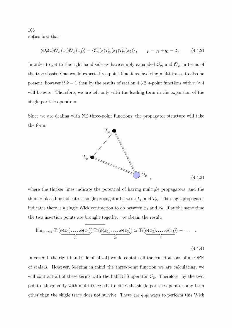
108notice first that

〈Op(x)Oq1(x1)Oq2(x2)〉 = 〈Op(x)Tq1(x1)Tq2(x2)〉 , p = q1 + q2 − 2 , (4.4.2)

In order to get to the right hand side we have simply expanded Oq1 and Oq2 in terms of

the trace basis. One would expect three-point functions involving multi-traces to also be

present, however if k = 1 then by the results of section 4.3.2 n-point functions with n ≥ 4

will be zero. Therefore, we are left only with the leading term in the expansion of the

single particle operators.

Since we are dealing with NE three-point functions, the propagator structure will take

the form:

Op

Tq1

Tq2

, (4.4.3)

where the thicker lines indicate the potential of having multiple propagators, and the

thinner black line indicates a single propagator between Tq1 and Tq2 . The single propagator

indicates there is a single Wick contraction to do between x1 and x2. If at the same time

the two insertion points are brought together, we obtain the result,

limx1→x2 Tr(φ(x1). . . . .φ(x1)︸ ︷︷ ︸q1

) Tr(φ(x2). . . . .φ(x2)︸ ︷︷ ︸q2

) ' Tr(φ(x2). . . . .φ(x2)︸ ︷︷ ︸p

) + . . . .

(4.4.4)

In general, the right hand side of (4.4.4) would contain all the contributions of an OPE

of scalars. However, keeping in mind the three-point function we are calculating, we

will contract all of these terms with the half-BPS operator Op. Therefore, by the two-

point orthogonality with multi-traces that defines the single particle operator, any term

other than the single trace does not survive. There are q1q2 ways to perform this Wick

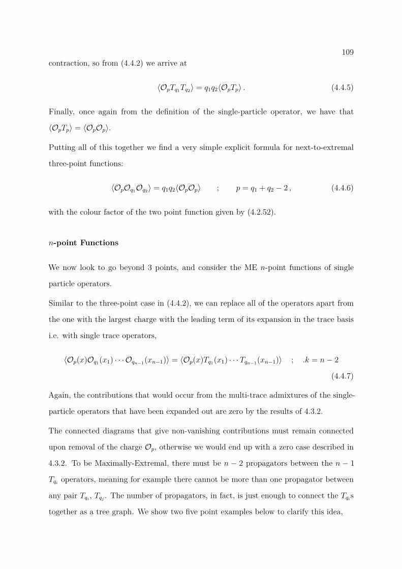
109contraction, so from (4.4.2) we arrive at

〈OpTq1Tq2〉 = q1q2〈OpTp〉 . (4.4.5)

Finally, once again from the definition of the single-particle operator, we have that

〈OpTp〉 = 〈OpOp〉.

Putting all of this together we find a very simple explicit formula for next-to-extremal

three-point functions:

〈OpOq1Oq2〉 = q1q2〈OpOp〉 ; p = q1 + q2 − 2 , (4.4.6)

with the colour factor of the two point function given by (4.2.52).

n-point Functions

We now look to go beyond 3 points, and consider the ME n-point functions of single

particle operators.

Similar to the three-point case in (4.4.2), we can replace all of the operators apart from

the one with the largest charge with the leading term of its expansion in the trace basis

i.e. with single trace operators,

〈Op(x)Oq1(x1) · · · Oqn−1(xn−1)〉 = 〈Op(x)Tq1(x1) · · ·Tqn−1(xn−1)〉 ; .k = n− 2

(4.4.7)

Again, the contributions that would occur from the multi-trace admixtures of the single-

particle operators that have been expanded out are zero by the results of 4.3.2.

The connected diagrams that give non-vanishing contributions must remain connected

upon removal of the charge Op, otherwise we would end up with a zero case described in

4.3.2. To be Maximally-Extremal, there must be n − 2 propagators between the n − 1

Tqi operators, meaning for example there cannot be more than one propagator between

any pair Tqi , Tqj . The number of propagators, in fact, is just enough to connect the Tqis

together as a tree graph. We show two five point examples below to clarify this idea,

110

OpTq1

Tq2

Tq3

Tq4

OpTq1

Tq2

Tq3

Tq4

(4.4.8)

In the first case, the tree we refer to above consists of Tq1 connected to Tq2 , Tq3 and Tq4 .

This is the maximum number of propagators that could have come off of Tq1 . In the

second diagram the tree consists of Tq1 connected to Tq2 and Tq4 , and Tq3 connected to

Tq4 .

So, the propagator structures contributing to an ME n-point correlator (4.4.7) contains a

sub-propagator structure which is a tree, T . To each tree one can associate a sequence of

length (n− 3) called the Prüfer sequence, which uniquely labels the propagator structure

of the tree linking the (n− 1) Tq operators. Using the structure of the trees associated

with Prüfer sequences, one can show that the pairwise computation of Wick contractions

represented by the trees can be given by

|W [T ]| =n−1∏i=1

qi(qi − 1) . . . (qi − di + 1). (4.4.9)

Here di corresponds to the number of propagator ends within the tree structure that

connects to operator Tqi . We shall provide more details about this point of view in

appendix D.

By performing the Wick contractions leaf by leaf on the tree as dictated by the Prüfer

algorithm, and by bringing the insertion points together at each stage, we can use the

same argument given in section 4.4.1 to argue that in the end gluing together the Tqis

will result in a single trace operator Tp together with higher trace terms. However, the

higher trace terms will not contribute in the full ME correlator as they will be limits of

near-extremal functions. Therefore, the entire connected part of the ME correlator can

111be written as a sum over trees, with the full sum multiplied by the two-point function

〈OpOp〉 to give:

〈Op(x)Oq1(x1) · · · Oqn−1(xn−1)〉connected = 〈OpOp〉( ∑trees T

|W [T ]| T (g)), (4.4.10)

where the sum is restricted to di ≥ 1 and ∑n−1i=1 di = 2(n − 2). Here |W[T ]| is given by

(4.4.9) and T (g) gives the corresponding spacetime structure. T (g) is constructed by

multiplying ∏n−1i=1 g

qi−din i by ∏i,j gij where the second product is over pairs of insertion

points connected by propagators dictated by the propagator structure of T .

Note that the counting of trees of n − 1 points is well studied, and given by Cayley’s

formula:

(n−1)n−3 . (4.4.11)

Finally, many trees correspond to the same arrangement of degrees di where i = 1, . . . , n−1.

Therefore, many of the trees will have the same value of |W[T ]|.9 This degeneracy is

counted by the multinomial coefficient given by

(n− 3)!∏n−1i=1 (di − 1)! . (4.4.12)

Disconnected Contributions

The maximally extremal (ME) correlators can have disconnected contributions even in

the SU(N) theory. To see what the disconnected pieces look like, we can use similar

reasoning to that given in (4.3.17) and the discussion around it. We give the argument

here for completeness.

Without loss of generality, we shall say that r of the (n− 1) Tq operators form one of the

disconnected pieces, and the other piece contains Op, Tr+1, . . . , Tn−1. Upon the removal

of Op, the rest of Tr+1, . . . , Tn−1 must remain connected, otherwise we would get a near

extremal diagram which we showed in 4.3.2 is equal to zero. The minimal way for this

9It is interesting to note, therefore, that a tree is not specified uniquely by giving the number ofpropagator ends that reach each point. It is only unique when the configuration of bridges is alsospecified.

112to occur is for the other operators to be connected like a tree diagram themselves. This

would lead the number of bridges between these operators, and not Op, to be

kR = 12

−p+n−1∑i=r+1

qi

≥ n− r − 2. (4.4.13)

The condition imposed by looking at Maximally-Extremal correlators is

k = 12

(−p+

n−1∑i=1

qi

)= n− 2 . (4.4.14)

Therefore, using (4.4.13) with (4.4.14) we get

12

r∑i=1

qi = n− 2− kR ≤ r . (4.4.15)

The final inequality, specifically looking at 12∑ri=1 qi ≤ r, indicates that the only way

for disconnected propagator structures to give non-zero contributions to (4.4.7) is if the

operators not connected to Op are all single particle operators of charge two. Let K be

the number of operators that are disconnected from Op, all of which are O2 operators,

and K ≥ 2. Let k1, . . . , kr label the partitions of K such that there are no 1’s, meaning

ki ≥ 2 for all i and ∑ri=1 ki = K. The disconnected part of the correlation function is

given by

〈(K∏i=1O2

)OqK+1 . . .Oqn−1Op〉discon. =

∑k1,...,kr`K

〈k1∏i=1O2〉 . . . 〈

kr∏i=1O2〉〈OqK+1 . . .Oqn−1Op〉conn.

(4.4.16)

We will conclude this section with some simple examples described below.

4-point Functions

Using (4.4.11), we see there are three possible trees for the operators. Referring to

the number of legs at positions i = 1, 2, 3 given by di, the three trees correspond to

d1 = 2, d2,3 = 1 and the two other unique permutations of this. There is no degeneracy,

113as can be seen by (4.4.12), therefore using (4.4.10) the full result is given by

〈OpOq1Oq2Oq3〉connected = q1q2q3 〈OpOp〉[(q1−1)gq1−2

41 gq2−142 gq3−1

43 g12g13+ (4.4.17)

(q2−1)gq1−141 gq2−2

42 gq3−143 g12g23 + (q3−1)gq1−1

41 gq2−142 gq3−2

43 g13g23

].

5-point Functions

Again using (4.4.11), the number of trees is given by 42 = 16, and this is the first number

of points with degeneracy. There are four non-degenerate trees given by

d1 = 3 , dj=2,3,4 = 1 ; d2 = 3 , dj=1,3,4 = 1 ; d3 = 3 , dj=1,2,4 = 1 ; d4 = 3 , dj=1,2,3 = 1.

(4.4.18)

On top of that, there are the following six configurations that have degeneracy two

di=1,2 = 2 , di=3,4 = 1 ; di=1,3 = 2 , di=2,4 = 1 (4.4.19)

di=1,4 = 2 , di=2,3 = 1 ; di=2,3 = 2 , di=1,4 = 1

di=2,4 = 2 , di=1,3 = 1 ; di=3,4 = 2 , di=1,2 = 1.

It is worth noting that the contribution of some of the trees might vanish for low charges.

For example, consider the case q1 = 2; the diagram associated to d1 = 3, dj=2,3,4 = 1

contributes q1q2q3q4(q1−1)(q1−2). This vanishes the case of q1 = 2. In fact, if we consider

the correlator 〈O2O2O2O2O2〉 all of the non-degenerate diagrams vanish and we are left

with the degenerate trees given above, all contributing with coefficient q1q2q3q4 = 16.

4.4.2 Next-to-Maximally-Extremal Correlators

The next correlation functions to consider are the next-to-maximally-extremal functions

(NME). These are the n-point correlators given by

〈Op(x)Oq1(x1) . . .Oqn−1(xn−1)〉 ; k = n− 1 ; k = 12(−p+

∑qi) . (4.4.20)

114Once again, it is worth noting the difference between the two different associations with

the term “extremality”. The NME functions refer to the set of n-point correlators that

have the second lowest value of k for which they do not vanish. However, this is not a

fixed value of k for all n. At three points, the N2E three point functions are the next-

to-maximally-extremal three point functions. At four points the N3E functions are the

next-to-maximally-extremal four-point functions.

To begin we will discuss three-point next-to-maximally-extremal functions, and provide

an explicit, closed formula for these functions. We will then move on to comment on

n-point NME correlators.

3-Point Functions

Starting with n = 3 we are studying next-next-to-extremal three-point functions

〈Op(x)Oq1(x1)Oq2(x2)〉 ; p = q1 + q2 − 4. (4.4.21)

We will see below that these correlation functions can also be related to the two-point

function 〈OpOp〉, but with a more complicated pre-factor than in (4.4.6) consisting of

non-factorisable polynomials.

Once again, to continue we replace Oq1 and Oq2 by their respective expansions in the trace

basis. For this case, the expansion will truncate for any term involving higher than double-

trace operators at a single point with all other terms vanishing due to the now familiar

near-extremal argument. Furthermore, double trace operators can be replaced directly

with double particle operators (meaning the product of two single particle operators)

since any other terms would vanish. Therefore, we end up with the following expansion

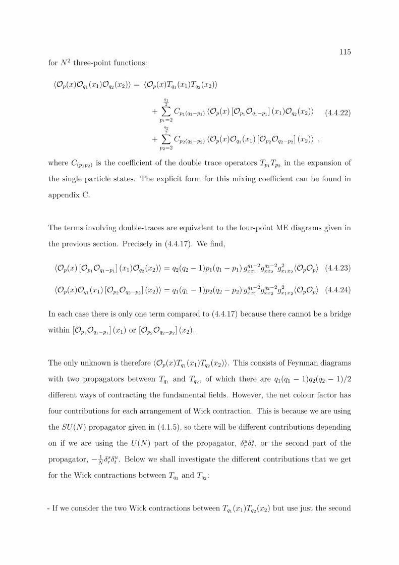
115for N2 three-point functions:

〈Op(x)Oq1(x1)Oq2(x2)〉 = 〈Op(x)Tq1(x1)Tq2(x2)〉

+q12∑

p1=2Cp1(q1−p1) 〈Op(x) [Op1Oq1−p1 ] (x1)Oq2(x2)〉

+q22∑

p2=2Cp2(q2−p2) 〈Op(x)Oq1(x1) [Op2Oq2−p2 ] (x2)〉 ,

(4.4.22)

where C(p1p2) is the coefficient of the double trace operators Tp1Tp2 in the expansion of

the single particle states. The explicit form for this mixing coefficient can be found in

appendix C.

The terms involving double-traces are equivalent to the four-point ME diagrams given in

the previous section. Precisely in (4.4.17). We find,

〈Op(x) [Op1Oq1−p1 ] (x1)Oq2(x2)〉 = q2(q2 − 1)p1(q1 − p1) gq1−2xx1 gq2−2

xx2 g2x1x2〈OpOp〉 (4.4.23)

〈Op(x)Oq1(x1) [Op2Oq2−p2 ] (x2)〉 = q1(q1 − 1)p2(q2 − p2) gq1−2xx1 gq2−2

xx2 g2x1x2〈OpOp〉 (4.4.24)

In each case there is only one term compared to (4.4.17) because there cannot be a bridge

within [Op1Oq1−p1 ] (x1) or [Op2Oq2−p2 ] (x2).

The only unknown is therefore 〈Op(x)Tq1(x1)Tq2(x2)〉. This consists of Feynman diagrams

with two propagators between Tq1 and Tq2 , of which there are q1(q1 − 1)q2(q2 − 1)/2

different ways of contracting the fundamental fields. However, the net colour factor has

four contributions for each arrangement of Wick contraction. This is because we are using

the SU(N) propagator given in (4.1.5), so there will be different contributions depending

on if we are using the U(N) part of the propagator, δur δst , or the second part of the

propagator, − 1Nδsrδ

ut . Below we shall investigate the different contributions that we get

for the Wick contractions between Tq1 and Tq2 :

- If we consider the two Wick contractions between Tq1(x1)Tq2(x2) but use just the second

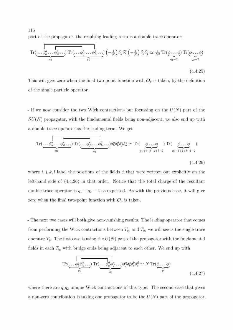
116part of the propagator, the resulting leading term is a double trace operator:

Tr(. . . φab . . . φcd . . .︸ ︷︷ ︸q1

) Tr(. . . φef . . . φgh . . .︸ ︷︷ ︸

q2

)(− 1N

)δab δ

gh

(− 1N

)δcdδ

ef ' 1

N2 Tr(φ . . . φ︸ ︷︷ ︸q1−2

) Tr(φ . . . φ︸ ︷︷ ︸q2−2

)

(4.4.25)

This will give zero when the final two-point function with Op is taken, by the definition

of the single particle operator.

- If we now consider the two Wick contractions but focussing on the U(N) part of the

SU(N) propagator, with the fundamental fields being non-adjacent, we also end up with

a double trace operator as the leading term. We get

Tr(. . . φab . . . φcd . . .︸ ︷︷ ︸q1

) Tr(. . . φef . . . φgh . . .︸ ︷︷ ︸

q2

)δahδgb δcfδ

ed ' Tr( φ . . . φ︸ ︷︷ ︸

q1+i−j−k+l−2

) Tr( φ . . . φ︸ ︷︷ ︸q2−i+j+k−l−2

)

(4.4.26)

where i, j, k, l label the positions of the fields φ that were written out explicitly on the

left-hand side of (4.4.26) in that order. Notice that the total charge of the resultant

double trace operator is q1 + q2 − 4 as expected. As with the previous case, it will give

zero when the final two-point function with Op is taken.

- The next two cases will both give non-vanishing results. The leading operator that comes

from performing the Wick contractions between Tq1 and Tq2 we will see is the single-trace

operator Tp. The first case is using the U(N) part of the propagator with the fundamental

fields in each Tqi with bridge ends being adjacent to each other. We end up with

Tr(. . . φabφbc . . .︸ ︷︷ ︸q1

) Tr(. . . φdeφef . . .︸ ︷︷ ︸q2

)δafδebδbeδdc ' N Tr(φ . . . φ︸ ︷︷ ︸p

)

(4.4.27)

where there are q1q2 unique Wick contractions of this type. The second case that gives

a non-zero contribution is taking one propagator to be the U(N) part of the propagator,

117and the other to be the second part of the SU(N) propagator giving

Tr(. . . φab . . . φcd . . .︸ ︷︷ ︸q1

) Tr(. . . φef . . . φgh . . .︸ ︷︷ ︸

q2

)(−δahδ

gb

1Nδcdδ

ef − 1

Nδab δ

ghδcfδ

ed

)' − 2

NTr(φ . . . φ︸ ︷︷ ︸

p

)

(4.4.28)

The number of non-zero contractions of this type is given by q1(q1 − 1)q2(q2 − 1)/2.

So, upon inputting (4.4.27) and (4.4.28) into a vev with Op and using the fact that

〈TpOp〉 = 〈OpOp〉 we get the final result

〈Tq1Tq2Op〉 = q1q2

[N − (q1 − 1)(q2 − 1)

N

]〈OpOp〉 . (4.4.29)

Inputting the calculations described above into (4.4.22) yields an explicit formula for the

N2 extremal three-point functions of single particle operators

〈Op(x)Oq1(x1)Oq2(x2)〉 = 〈OpOp〉q1q2

[N − (q1 − 1)(q2 − 1)

N

]+

b q12 c∑

p1=2Cp1(q1−p1)q2(q2 − 1)p1(q1 − p1) +

b q22 c∑

p2=2Cp2(q2−p2)q1(q1 − 1)p2(q2 − p2)

. (4.4.30)

The two sums are symmetric and can be performed with the explicit knowledge of Cp1(q1−p1)

given in appendix C. We find

b q12 c∑

p1=2Cp1(q1−p1)p1(q1 − p1) =

q1

2N(q1 − 2)

[2N2 + (q1 − 1)2N + 2(q1 − 2)2 + 2(q1 − 1)2N(N)q1

(N − q1 + 1)q1 − (N)q1

](4.4.31)

n-Point Functions

Whilst we are not necessarily able to provide a closed formula for n-point NME functions,

the method described above can be generalised to any point. We provide a sketch of how

the computation goes here.

The definition of k = 12(−p+∑

qi) = n− 1 selects an operator Op to be special in some

way, and we call the others “light". The calculation begins by expanding all these “light"

118operators in terms of the trace basis, where it should be clear that almost all terms in

the expansion vanish since they produce correlators equivalent to near-extremal higher

point diagrams. The result is the following generalisation of the three-point expansion in

(4.4.22), namely

〈Oq1 . . .Oqn−1Op〉 = 〈Tq1 . . . Tqn−1Op(xn)〉+

n−1∑i=1

b qi2 c∑pi=2

Cpi(qi−pi) 〈Oq1 . . .Oqi−1 [OpiOqi−pi ]Oqi+1 . . .Op(xn)〉 .

(4.4.32)

We can think of (4.4.32) as a separate equation for each contributing Feynman diagram

independently. Note that the correlators in the sum are all contributions to n+ 1-point

Nn−1-extremal correlators, which are maximally extremal, so we have formulae for them in

section 4.4.1. The first term can then be computed by doing the partial Wick contractions,

n− 1 in total, on the single trace operators Tp1 . . . Tpn−1 only keeping the relevant terms,

just as was done in the three-point case in the discussion above (4.4.29).

4.4.3 On correlators with lower extremality

In section 4.4.1, we defined how to classify free theory correlators according to their

degree of extremality with respect to the maximally-extremal correlator. The maximally-

extremal n-point correlators were defined to be the simplest non-vanishing correlators,

which are those which satisfy k = n− 2, as for k ≤ n− 3 we showed in 4.3 they vanish.

These functions can be computed in terms of tree graphs, and the charge dependence

on p and the qis fully factorises out for each tree graph, with the factor having a clean

interpretation. The NME functions in section 4.4.2 showed more structure. They were not

as simple to calculate directly, however a closed formula was found in the end for the three-

point functions. We would expect that NNME functions will have ever more structure,

and so on for higher extremality. Here we will explicitly show that the complexity of

NNME is already evident in the three-point functions.

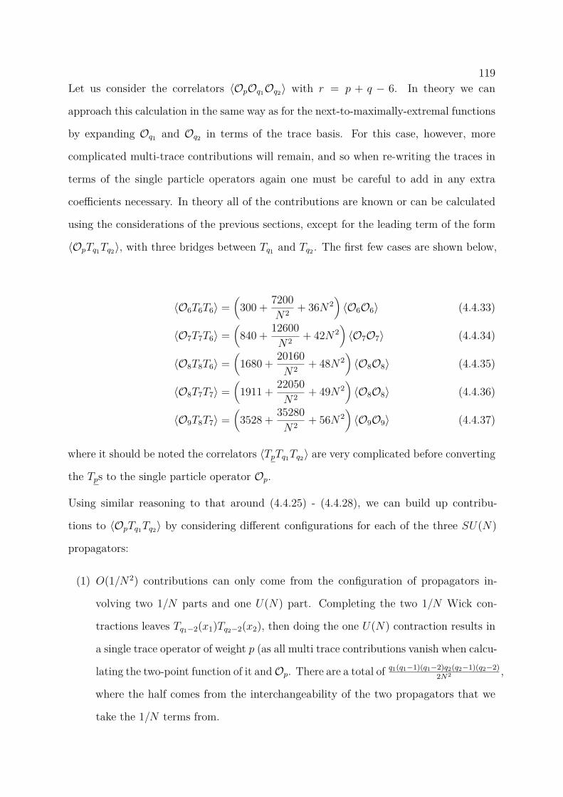
119Let us consider the correlators 〈OpOq1Oq2〉 with r = p + q − 6. In theory we can

approach this calculation in the same way as for the next-to-maximally-extremal functions

by expanding Oq1 and Oq2 in terms of the trace basis. For this case, however, more

complicated multi-trace contributions will remain, and so when re-writing the traces in

terms of the single particle operators again one must be careful to add in any extra

coefficients necessary. In theory all of the contributions are known or can be calculated

using the considerations of the previous sections, except for the leading term of the form

〈OpTq1Tq2〉, with three bridges between Tq1 and Tq2 . The first few cases are shown below,

〈O6T6T6〉 =(

300 + 7200N2 + 36N2

)〈O6O6〉 (4.4.33)

〈O7T7T6〉 =(

840 + 12600N2 + 42N2

)〈O7O7〉 (4.4.34)

〈O8T8T6〉 =(

1680 + 20160N2 + 48N2

)〈O8O8〉 (4.4.35)

〈O8T7T7〉 =(

1911 + 22050N2 + 49N2

)〈O8O8〉 (4.4.36)

〈O9T8T7〉 =(

3528 + 35280N2 + 56N2

)〈O9O9〉 (4.4.37)

where it should be noted the correlators 〈TpTq1Tq2〉 are very complicated before converting

the Tps to the single particle operator Op.

Using similar reasoning to that around (4.4.25) - (4.4.28), we can build up contribu-

tions to 〈OpTq1Tq2〉 by considering different configurations for each of the three SU(N)

propagators:

(1) O(1/N2) contributions can only come from the configuration of propagators in-

volving two 1/N parts and one U(N) part. Completing the two 1/N Wick con-

tractions leaves Tq1−2(x1)Tq2−2(x2), then doing the one U(N) contraction results in

a single trace operator of weight p (as all multi trace contributions vanish when calcu-

lating the two-point function of it andOp. There are a total of q1(q1−1)(q1−2)q2(q2−1)(q2−2)2N2 ,

where the half comes from the interchangeability of the two propagators that we

take the 1/N terms from.

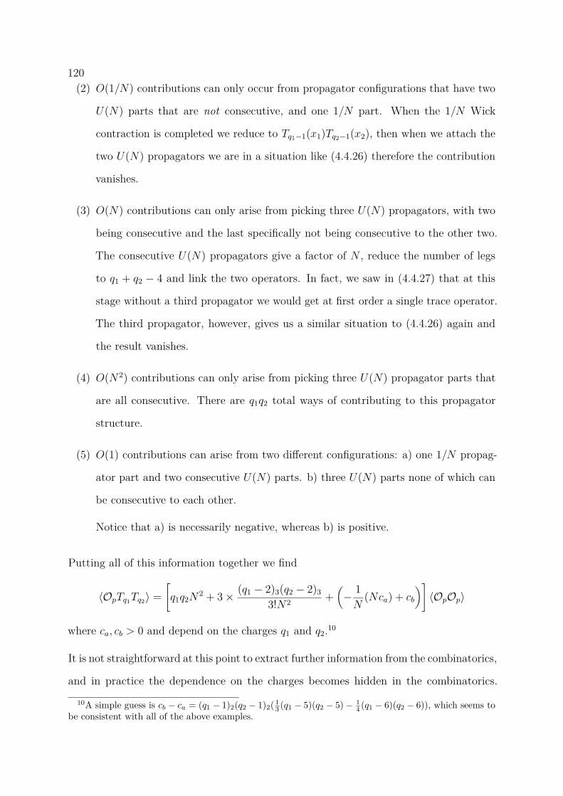
120(2) O(1/N) contributions can only occur from propagator configurations that have two

U(N) parts that are not consecutive, and one 1/N part. When the 1/N Wick

contraction is completed we reduce to Tq1−1(x1)Tq2−1(x2), then when we attach the

two U(N) propagators we are in a situation like (4.4.26) therefore the contribution

vanishes.

(3) O(N) contributions can only arise from picking three U(N) propagators, with two

being consecutive and the last specifically not being consecutive to the other two.

The consecutive U(N) propagators give a factor of N , reduce the number of legs

to q1 + q2 − 4 and link the two operators. In fact, we saw in (4.4.27) that at this

stage without a third propagator we would get at first order a single trace operator.

The third propagator, however, gives us a similar situation to (4.4.26) again and

the result vanishes.

(4) O(N2) contributions can only arise from picking three U(N) propagator parts that

are all consecutive. There are q1q2 total ways of contributing to this propagator

structure.

(5) O(1) contributions can arise from two different configurations: a) one 1/N propag-

ator part and two consecutive U(N) parts. b) three U(N) parts none of which can

be consecutive to each other.

Notice that a) is necessarily negative, whereas b) is positive.

Putting all of this information together we find

〈OpTq1Tq2〉 =[q1q2N

2 + 3× (q1 − 2)3(q2 − 2)3

3!N2 +(− 1N

(Nca) + cb

)]〈OpOp〉

where ca, cb > 0 and depend on the charges q1 and q2.10

It is not straightforward at this point to extract further information from the combinatorics,

and in practice the dependence on the charges becomes hidden in the combinatorics.

10A simple guess is cb − ca = (q1 − 1)2(q2 − 1)2( 13 (q1 − 5)(q2 − 5)− 1

4 (q1 − 6)(q2 − 6)), which seems tobe consistent with all of the above examples.

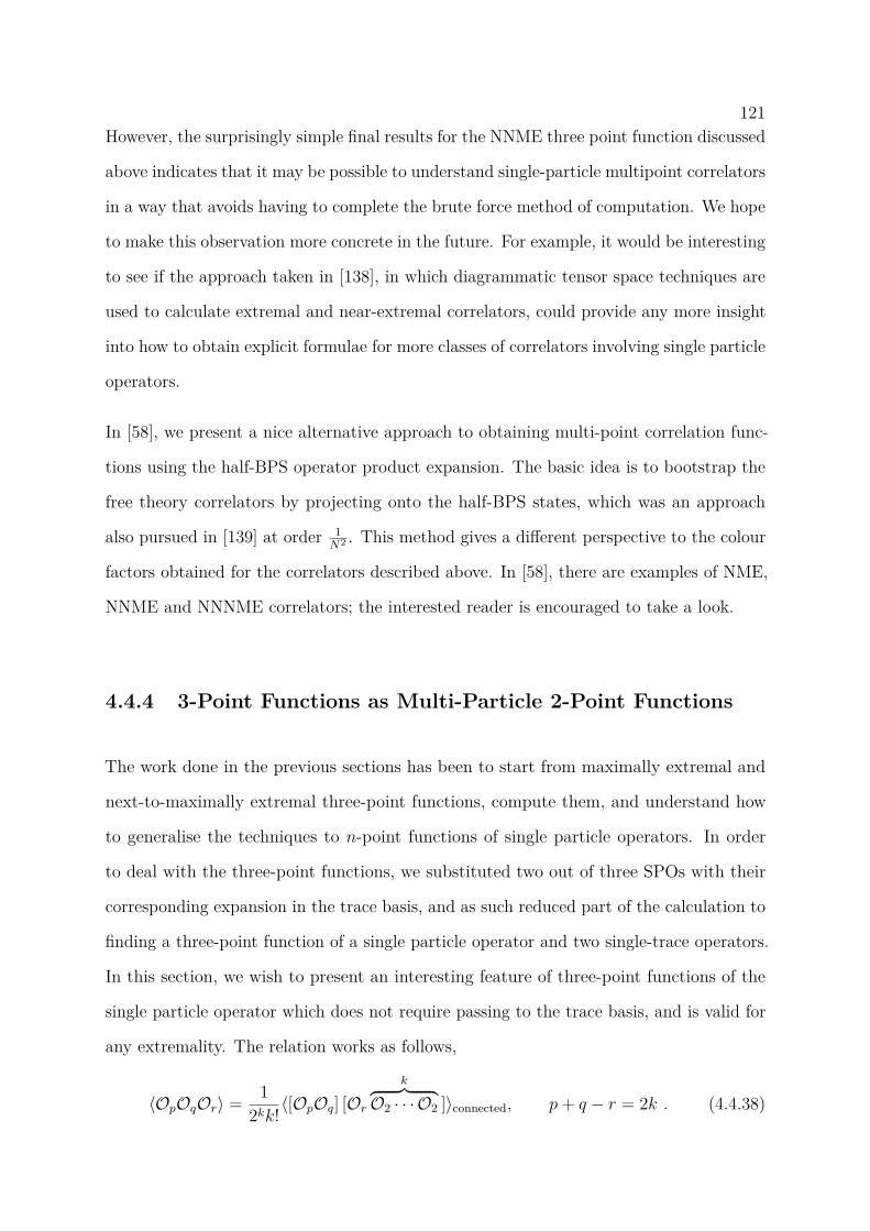
121However, the surprisingly simple final results for the NNME three point function discussed

above indicates that it may be possible to understand single-particle multipoint correlators

in a way that avoids having to complete the brute force method of computation. We hope

to make this observation more concrete in the future. For example, it would be interesting

to see if the approach taken in [138], in which diagrammatic tensor space techniques are

used to calculate extremal and near-extremal correlators, could provide any more insight

into how to obtain explicit formulae for more classes of correlators involving single particle

operators.

In [58], we present a nice alternative approach to obtaining multi-point correlation func-

tions using the half-BPS operator product expansion. The basic idea is to bootstrap the

free theory correlators by projecting onto the half-BPS states, which was an approach

also pursued in [139] at order 1N2 . This method gives a different perspective to the colour

factors obtained for the correlators described above. In [58], there are examples of NME,

NNME and NNNME correlators; the interested reader is encouraged to take a look.

4.4.4 3-Point Functions as Multi-Particle 2-Point Functions

The work done in the previous sections has been to start from maximally extremal and

next-to-maximally extremal three-point functions, compute them, and understand how

to generalise the techniques to n-point functions of single particle operators. In order

to deal with the three-point functions, we substituted two out of three SPOs with their

corresponding expansion in the trace basis, and as such reduced part of the calculation to

finding a three-point function of a single particle operator and two single-trace operators.

In this section, we wish to present an interesting feature of three-point functions of the

single particle operator which does not require passing to the trace basis, and is valid for

any extremality. The relation works as follows,

〈OpOqOr〉 = 12kk!〈[OpOq] [Or

k︷ ︸︸ ︷O2 · · · O2 ]〉connected, p+ q − r = 2k . (4.4.38)

122where the equality is for the color factor of the left hand side being the same as that of a

two-point function of multi-particle operators of SPOs on the right hand side.

Let us first illustrate the case k = 3 with the following picture,

Op

Oq

Or

[O2 O2 O2 Or]

[Op Oq]

(4.4.39)

The diagram on the left is the single diagram contributing to 〈OpOqOr〉, whereas the one

on the right is the only type of diagram contributing to 〈[OpOq] [OrO2O2O2 ]〉.

To show (4.4.38), consider where the two legs out of an O2 can end. They can not go

to Or as they are at the same point. If they both went to Op , this would result in a

diagram of the form of a dumbbell in (4.3.1) (centered around Op) which thus vanishes.

Similarly if both legs go to Oq. The only exception to this is if p or q equals two in which

case you can have a completely disconnected contribution, however the statement (4.4.38)

is for the connected diagram so we do not need to consider this case. Therefore, the only

remaining possibility is that one leg goes to Op and one to Oq resulting in the diagram

shown on the right. There are clearly 2kk! different but equivalent diagrams of this sort,

arising from the k! possibilities of swapping the propagators from Op to the O2s and from

the cyclic symmetry around each O2.

The colour factor of 〈OpOqOr〉 is the same as one of the equivalent configuration of

〈[OpOq] [OrO2 . . .O2 ]〉 described above. This follows from the fact that

(4.4.40)

123which concludes our proof of (4.4.38).11

While the right hand side of (4.4.38) is restricted to the connected part of the two point

function (thinking of it as a limit of a higher point function) rather than the full two-point

function, we need this distinction only when p or q equals 2 and k = 1. In this case we

have

〈OqO2Oq〉 = 12 (〈[OqO2] [OqO2]〉 − 〈OqOq〉 〈O2O2〉) . (4.4.41)

It is worth noting that the condition giving the value of k in (4.4.38) is dependent on the

order of Op, Oq and Or; in particular it distinguishes Or from the other two operators.

However the colour factor of the three-point function does not depend on this ordering.

For example, consider the three point function of O3, O4 and O5, we can have three

multi-particle two-point functions with k = 1, 2, 3 respectively,

〈O3O4O5〉 = 〈O3O5O4〉 = 〈O4O5O3〉 = 60∏4i=1(N2 − i2)

N(5 +N2)

= = =

12 〈[O3O4] [O5O2]〉 1

8 〈[O3O5] [O4O2O2]〉 148 〈[O4O5] [O3O2O2O2]〉

(4.4.42)

All three multi-particle two-point functions are then equal!.

We conclude that for a triplet of single-particle operators all multi-particle two-point

functions which correspond to different dispositions of the three SPOs give the same color

factor up to a multiplicity counted by 2kk!.

While the discussion above required Op and Oq to be SPOs, it nowhere relied on Or to

be an SPO. Thus the following more general relation holds for any half-BPS operator

Tr1,...,rl :

〈OpOqTr1,...,rl〉 = 12kk!〈[OpOq] [Tr1,...,rl

k︷ ︸︸ ︷O2 · · · O2 ]〉|connected, (4.4.43)

with r1 + ...+ rl = r and p+ q − r = 2k.

11The ideas of our proof here can be generalised to multipoint correlators as well. For example thosewhich are equivalent to the l.h.s. of (4.4.43).

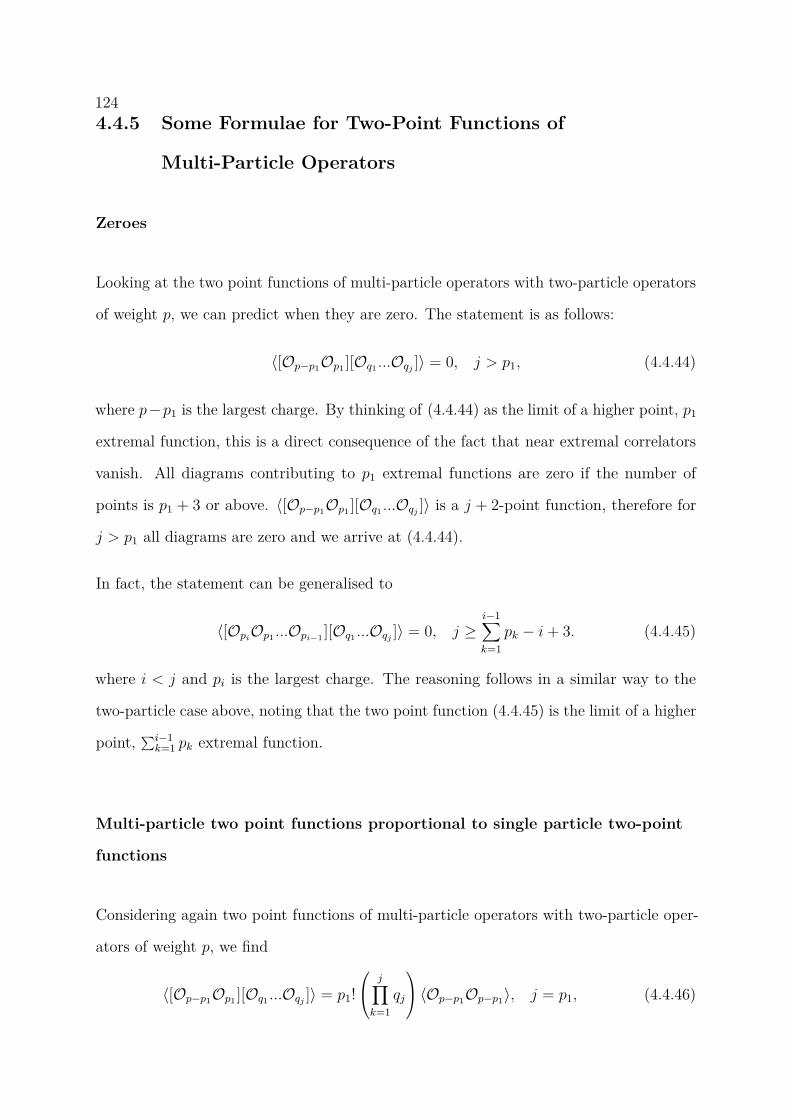
1244.4.5 Some Formulae for Two-Point Functions of

Multi-Particle Operators

Zeroes

Looking at the two point functions of multi-particle operators with two-particle operators

of weight p, we can predict when they are zero. The statement is as follows:

〈[Op−p1Op1 ][Oq1 ...Oqj ]〉 = 0, j > p1, (4.4.44)

where p−p1 is the largest charge. By thinking of (4.4.44) as the limit of a higher point, p1

extremal function, this is a direct consequence of the fact that near extremal correlators

vanish. All diagrams contributing to p1 extremal functions are zero if the number of

points is p1 + 3 or above. 〈[Op−p1Op1 ][Oq1 ...Oqj ]〉 is a j + 2-point function, therefore for

j > p1 all diagrams are zero and we arrive at (4.4.44).

In fact, the statement can be generalised to

〈[OpiOp1 ...Opi−1 ][Oq1 ...Oqj ]〉 = 0, j ≥i−1∑k=1

pk − i+ 3. (4.4.45)

where i < j and pi is the largest charge. The reasoning follows in a similar way to the

two-particle case above, noting that the two point function (4.4.45) is the limit of a higher

point, ∑i−1k=1 pk extremal function.

Multi-particle two point functions proportional to single particle two-point

functions

Considering again two point functions of multi-particle operators with two-particle oper-

ators of weight p, we find

〈[Op−p1Op1 ][Oq1 ...Oqj ]〉 = p1! j∏k=1

qj

〈Op−p1Op−p1〉, j = p1, (4.4.46)

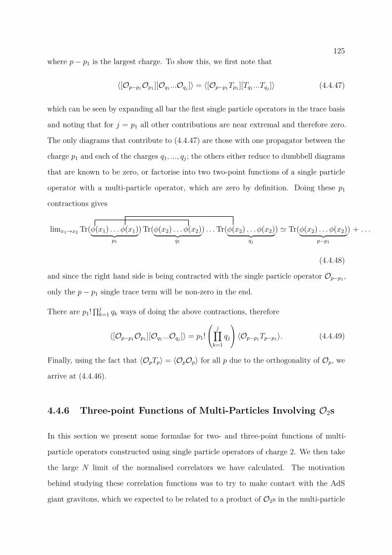
125where p− p1 is the largest charge. To show this, we first note that

〈[Op−p1Op1 ][Oq1 ...Oqj ]〉 = 〈[Op−p1Tp1 ][Tq1 ...Tqj ]〉 (4.4.47)

which can be seen by expanding all bar the first single particle operators in the trace basis

and noting that for j = p1 all other contributions are near extremal and therefore zero.

The only diagrams that contribute to (4.4.47) are those with one propagator between the

charge p1 and each of the charges q1, ..., qj; the others either reduce to dumbbell diagrams

that are known to be zero, or factorise into two two-point functions of a single particle

operator with a multi-particle operator, which are zero by definition. Doing these p1

contractions gives

limx1→x2 Tr(φ(x1) . . . φ(x1)︸ ︷︷ ︸p1

) Tr(φ(x2) . . . φ(x2)︸ ︷︷ ︸q1

) . . .Tr(φ(x2) . . . φ(x2)︸ ︷︷ ︸qj

) ' Tr(φ(x2) . . . φ(x2)︸ ︷︷ ︸p−p1

) + . . .

(4.4.48)

and since the right hand side is being contracted with the single particle operator Op−p1 ,

only the p− p1 single trace term will be non-zero in the end.

There are p1!∏jk=1 qk ways of doing the above contractions, therefore

〈[Op−p1Op1 ][Oq1 ...Oqj ]〉 = p1! j∏k=1

qj

〈Op−p1Tp−p1〉. (4.4.49)

Finally, using the fact that 〈OpTp〉 = 〈OpOp〉 for all p due to the orthogonality of Op, we

arrive at (4.4.46).

4.4.6 Three-point Functions of Multi-Particles Involving O2s

In this section we present some formulae for two- and three-point functions of multi-

particle operators constructed using single particle operators of charge 2. We then take

the large N limit of the normalised correlators we have calculated. The motivation

behind studying these correlation functions was to try to make contact with the AdS

giant gravitons, which we expected to be related to a product of O2s in the multi-particle

126basis. In the Schur basis the AdS giants are given by the Schur polynomial operators

associated to the completely symmetric Young diagram. By comparing to results detailed

in [140] we will see that these limits are in fact not in agreement with the AdS giant

graviton calculation on the string theory side. However, the explicit expressions for the

correlators may be useful in the future so we present them here even though they do not

have the interpretation we expected in the large N limit.

We begin by calculating the three point function of the form 〈O2[O2...O2][O2...O2]〉.

Firstly, from many examples we observe the two-point function of products of O2’s is

given by

〈[k︷ ︸︸ ︷

O2...O2][k︷ ︸︸ ︷

O2...O2]〉 = 2k−1k!〈O2O2〉k−1∏i=1

(2i− 1 +N2) (4.4.50)

= 22(k−1)k!(1

2(1 +N2))k−1〈O2O2〉. (4.4.51)

This particular two-point function will be useful for calculating the rest of the correlators

considered in this section. Note that for the rest of the section we shall use the variables

k and l to represent the number of O2 operators in a multi-particle operator, and q and

r for when we are referring to the total charge of the multi-particle operator.

The only non-zero correlators of the form 〈O2[

q2︷ ︸︸ ︷

O2...O2][

r2︷ ︸︸ ︷

O2...O2]〉 are those with q2 = r

2 = k

and q2 = k, r

2 = k − 1. The three-point functions are given by

〈O2[k︷ ︸︸ ︷

O2...O2][k−1︷ ︸︸ ︷O2...O2]〉 = 〈[

k︷ ︸︸ ︷O2...O2][

k︷ ︸︸ ︷O2...O2]〉, (4.4.52)

〈O2[k︷ ︸︸ ︷

O2...O2][k︷ ︸︸ ︷

O2...O2]〉 = 2 · 2k〈[k︷ ︸︸ ︷

O2...O2][k︷ ︸︸ ︷

O2...O2]〉. (4.4.53)

Relation (4.4.52) is clear from the point of view of the correlator as a limit of the 2k-

point function of O2’s. There cannot be a contributing diagram with a propagator

between the individual O2 and any of the k − 1 group of O2’s, as there is no consistent

propagator structure that can link the rest of the fields of the O2s. Therefore, the

diagrams contributing to (4.4.52) are the same as the diagrams contributing to the two-

127point function (4.4.50). The relation (4.4.53) comes from the same considerations as in

section 4.4.1, and the observation that

〈[k︷ ︸︸ ︷

O2...O2][k︷ ︸︸ ︷

T2...T2]〉 = 〈[k︷ ︸︸ ︷

O2...O2][k︷ ︸︸ ︷

O2...O2]〉,

which is a result of near-extremal correlators vanishing.

We consider the limit of the normalised three-point functions (4.4.52) and (4.4.53) whereN →∞, and q, r →∞ such that q′ = q

N, r′ = r

Nare fixed. We find the limit of (4.4.52)

is given by

〈O2[k︷ ︸︸ ︷

O2...O2][k−1︷ ︸︸ ︷O2...O2]〉√

〈O2O2〉〈[O2...O2︸ ︷︷ ︸k

][O2...O2︸ ︷︷ ︸k

]〉〈[O2...O2︸ ︷︷ ︸k−1

][O2...O2︸ ︷︷ ︸k−1

]〉→√q′N

2 , (4.4.54)

and the limit of (4.4.53) is given by

〈O2[k︷ ︸︸ ︷

O2...O2][k︷ ︸︸ ︷

O2...O2]〉√〈O2O2〉〈[O2...O2︸ ︷︷ ︸

k

][O2...O2︸ ︷︷ ︸k

]〉〈[O2...O2︸ ︷︷ ︸k

][O2...O2︸ ︷︷ ︸k

]〉→√

2 qN. (4.4.55)

In fact, equation (4.4.52) can be generalised to the following set of extremal three-point

functions:

〈[k︷ ︸︸ ︷

O2...O2][l︷ ︸︸ ︷

O2...O2][k+l︷ ︸︸ ︷

O2...O2]〉 = 〈[k+l︷ ︸︸ ︷

O2...O2][k+l︷ ︸︸ ︷

O2...O2]〉. (4.4.56)

There are no diagrams with propagators between the group of k O2’s and the group of

l O2’s, therefore the diagrams contributing to the three-point function on the left-hand

side of (4.4.56) are the same as the diagrams contributing to the two-point function on

the right-hand side of (4.4.56).

Now, taking the limit N →∞, but q →∞ such that q′ = qN

is fixed:

〈[k︷ ︸︸ ︷

O2...O2][l︷ ︸︸ ︷

O2...O2][k+l︷ ︸︸ ︷

O2...O2]〉√〈[O2...O2︸ ︷︷ ︸

k

][O2...O2︸ ︷︷ ︸k

]〉〈[O2...O2︸ ︷︷ ︸l

][O2...O2︸ ︷︷ ︸l

]〉〈[O2...O2︸ ︷︷ ︸k+l

][O2...O2︸ ︷︷ ︸k+l

]〉→√Nkq′k

2kk!

(=√lk

k!

). (4.4.57)

The 3-point function scales as N k2 . The expression for k = 1 is in agreement with (4.4.54).

128Finally, equation (4.4.53) can be generalised to the following set of next-to-extremal

three-point functions:

〈[k︷ ︸︸ ︷

O2...O2][l︷ ︸︸ ︷

O2...O2][k+l−1︷ ︸︸ ︷O2...O2]〉 = 2k · 2l〈[

k+l−1︷ ︸︸ ︷O2...O2][

k+l−1︷ ︸︸ ︷O2...O2]〉. (4.4.58)

This relies on the following;

〈[k︷ ︸︸ ︷

O2...O2][k︷ ︸︸ ︷

O2...O2]〉 = 〈[k︷ ︸︸ ︷

T2...T2][k︷ ︸︸ ︷

O2...O2]〉, (4.4.59)

〈[k︷ ︸︸ ︷

O2...O2][l︷ ︸︸ ︷

O2...O2][k+l−1︷ ︸︸ ︷O2...O2]〉 = 〈[

k︷ ︸︸ ︷T2...T2][

l︷ ︸︸ ︷T2...T2][

k+l−1︷ ︸︸ ︷O2...O2]〉, (4.4.60)

both of which are a consequence of the vanishing of near extremal functions.

Now, taking the limit N →∞, but q →∞ such that q′ = qN

is fixed:

〈[k︷ ︸︸ ︷

O2...O2][l︷ ︸︸ ︷

O2...O2][k+l−1︷ ︸︸ ︷O2...O2]〉√

〈[O2...O2︸ ︷︷ ︸k

][O2...O2︸ ︷︷ ︸k

]〉〈[O2...O2︸ ︷︷ ︸l

][O2...O2︸ ︷︷ ︸l

]〉〈[O2...O2︸ ︷︷ ︸k+l−1

][O2...O2︸ ︷︷ ︸k+l−1

]〉

→ 2kq′N√Nk−3q′k−1

2kk! = 2k√Nk−1q′k+1

2kk! , (4.4.61)

where q = 2l. The 3-point function scales as N k−12 , so is only finite for k = 1. As a sanity

check, the expression for k = 1 is in agreement with (4.4.55).

As mentioned at the beginning of this section, the limits can be compared to the string

theory calculation of the AdS giant gravitons given in [140]. They do not appear to agree,

therefore it seems that the products of O2 are not the right objects to compare to the

AdS giant graviton. It would be interesting to work out what object in the multi-particle

basis is related to the AdS giant graviton, but we shall leave this to future work.

4.5 Conclusions

In this chapter, we explored a new basis of half-BPS operators in N = 4 super Yang-

Mills. The basis was developed out of a need to be very precise when discussing the

definition of the operator dual to the single particle supergravity states on AdS5 × S5.

129Products of these single particle operators were then used to extend the basis to a full

multi-particle basis. We provide explicit formulae for these operators, and showed that

they interpolate between point-like gravitons and giant (sphere) gravitons in the relevant

limits, as they should. We then went on to consider free theory correlators of these

operators. A particularly interesting and useful result was found that stated all near-

extremal correlators of SPOs, namely n-point correlators with extremality degree strictly

less than n− 2, vanish. We would assume that this is tied to the conjecture given in [129]

that the corresponding supergravity couplings vanish. We then continued to consider the

maximally extremal correlators, which were nicely directly related to tree diagrams with

n − 1 vertices. The next-to-maximally extremal correlators were then studied; despite

finding that the complexity increases as the extremality is lowered, we found additional

simplicity compared to the single-trace correlators. Finally, we gave a few exact results of

two- and three-point functions of multi-particle operators, and particularly interestingly

proved a relation between the three-point functions of single particle operators and two-

point functions of multi-particle operators that held for all extremality.

It is interesting to revisit past discussions involving half-BPS operators, especially con-

cerning large N limits and the relation to string theory computations via AdS/CFT, in

the light of our new basis of SPOs. As we saw in section 4.2.3, the SPOs correctly inter-

polate between single trace operators and the operators conjectured to be dual to S5 giant

graviton operators in the relevant limit. In [140] the half-BPS three-point functions of two

giant graviton operators and one point-like graviton was performed and compared with

the analogous computation in gauge theory. The gauge theory was computed using two

large Schur polynomial operators and one single trace operator. The results were found to

not quite agree and it was conjectured the reason was related to the inability of the Schur

polynomials to correctly interpolate between giant and point-like gravitons. The SPOs on

the other hand do precisely interpolate between the two as show in section 4.2.3. However,

the extremal correlators of SPOs simply vanish! In [141] this issue was revisited and it

was argued that indeed there were subtleties in the extremal case which are not present

130in the next-to-extremal case. The NE three-point functions with two giant gravitons and

one point-like graviton were computed in gauge theory (using Schur polynomials for the

giant gravitons and single trace operators for the point-like operator) as well as in string

theory and this time found agreement. Since we have explicit formulae for the NE 3-point

functions we can check this agrees here also.

We start with the next-to-extremal three-point function of unit normalised single particle

operators. From (4.4.6) we have

〈OpOqOr〉√〈OpOp〉〈OqOq〉〈OrOr〉

= pq

√√√√ 〈OrOr〉〈OpOp〉〈OqOq〉

, p+ q = r + 2. (4.5.1)

Now consider the limit N → ∞ with p staying finite, but q, r → ∞ such that q′ =

q/N, r′ = r/N are fixed. Taking the appropriate limits of the two point functions (4.2.52)

we find

〈OpOqOr〉√〈OpOp〉〈OqOq〉〈OrOr〉

→ √p rN

(1− r

N

) p−22, p+ q = r + 2 (4.5.2)

which is in precise agreement with [141].

We can also compute the normalised next-to-next-to-extremal three-point function given

by (4.4.30)-(4.4.31) in the same limit, N →∞ with p, q′ = q/N, r′ = r/N fixed

〈OpOqOr〉√〈OpOp〉〈OqOq〉〈OrOr〉

→ √p rN

(1− r

N

)p−42(

1− (p− 1)r2N

), p+ q = r + 4.

(4.5.3)

It would be interesting to compare with the corresponding string theory computation.

We shall provide some examples of interesting paths that could lead to the continuation

of this work in Chapter 6.

Chapter 5

A Note on N2MHV Yangian

Invariants for N = 4 SYM

5.1 Introduction

Yangian invariants are the basic building blocks of many quantities of interest related

to amplitudes in N = 4 super Yang-Mills (see for example [43–45, 64, 142–145]). Some

examples of the quantities they can be used to construct include any tree-level amplitude

which can be written as a linear combination of Yangian invariants [146], and any lead-

ing singularity of a loop level integrand which are themselves Yangian invariants [147].

Therefore, a full understanding of all Yangian invariant functions and their properties

would be extremely useful. There have been considerable steps made recently in under-

standing these functions, for example all positive n-particle NkMHV Yangian invariants

with n = 5k were classified in [148]. Furthermore, all rational m = 2 (corresponding to

the toy model of N = 4 SYM) Yangian invariants were classified very nicely in terms of

generalised triangles inside the m = 2 amplituhedron [80].

In Section 2.3 we introduced the five particle R invariant in the context of the n-point

NMHV superamplitude integrand, and showed that it can be written in bosonised dual

momentum superspace co-ordinates (or amplituhedron coordinates) as the following dual

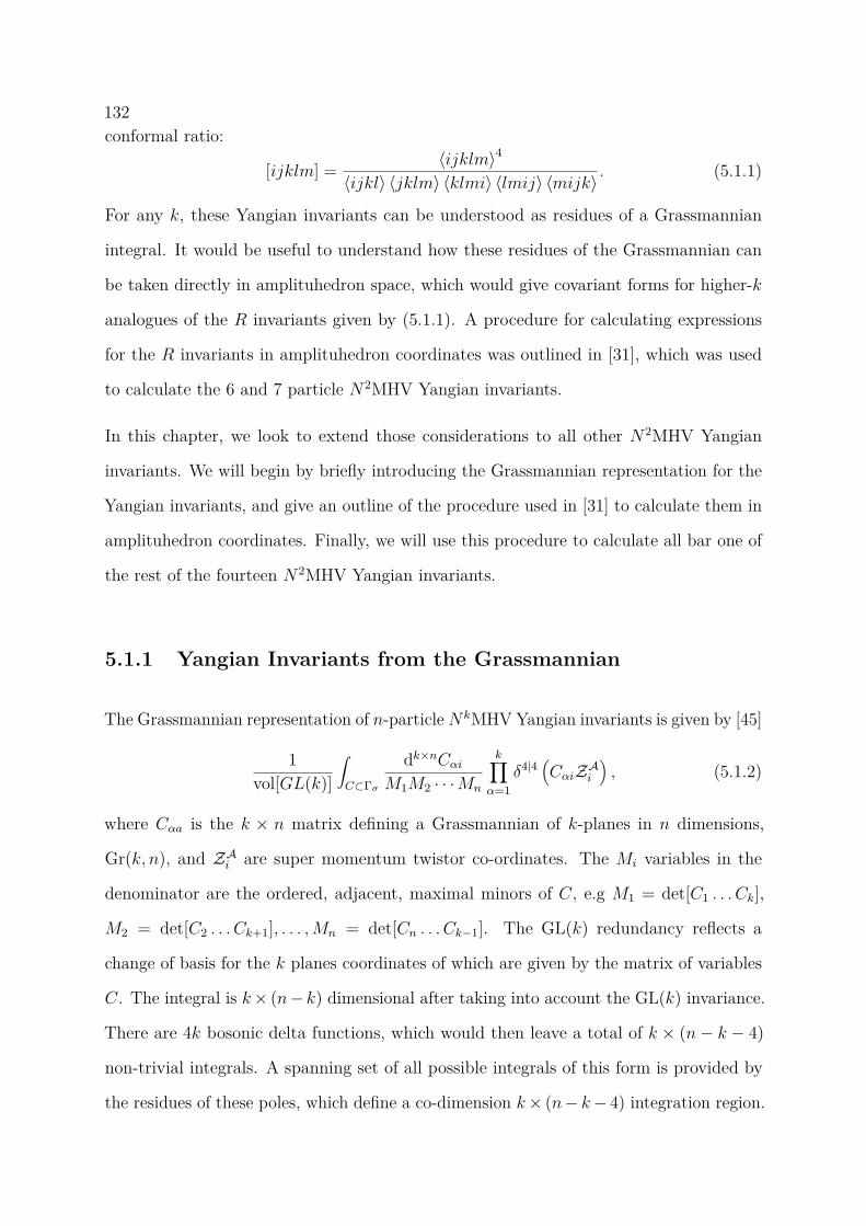
132conformal ratio:

[ijklm] = 〈ijklm〉4

〈ijkl〉 〈jklm〉 〈klmi〉 〈lmij〉 〈mijk〉. (5.1.1)

For any k, these Yangian invariants can be understood as residues of a Grassmannian

integral. It would be useful to understand how these residues of the Grassmannian can

be taken directly in amplituhedron space, which would give covariant forms for higher-k

analogues of the R invariants given by (5.1.1). A procedure for calculating expressions

for the R invariants in amplituhedron coordinates was outlined in [31], which was used

to calculate the 6 and 7 particle N2MHV Yangian invariants.

In this chapter, we look to extend those considerations to all other N2MHV Yangian

invariants. We will begin by briefly introducing the Grassmannian representation for the

Yangian invariants, and give an outline of the procedure used in [31] to calculate them in

amplituhedron coordinates. Finally, we will use this procedure to calculate all bar one of

the rest of the fourteen N2MHV Yangian invariants.

5.1.1 Yangian Invariants from the Grassmannian

The Grassmannian representation of n-particleNkMHV Yangian invariants is given by [45]

1vol[GL(k)]

∫C⊂Γσ

dk×nCαiM1M2 · · ·Mn

k∏α=1

δ4|4(CαiZAi

), (5.1.2)

where Cαa is the k × n matrix defining a Grassmannian of k-planes in n dimensions,

Gr(k, n), and ZAi are super momentum twistor co-ordinates. The Mi variables in the

denominator are the ordered, adjacent, maximal minors of C, e.g M1 = det[C1 . . . Ck],

M2 = det[C2 . . . Ck+1], . . . ,Mn = det[Cn . . . Ck−1]. The GL(k) redundancy reflects a

change of basis for the k planes coordinates of which are given by the matrix of variables

C. The integral is k× (n− k) dimensional after taking into account the GL(k) invariance.

There are 4k bosonic delta functions, which would then leave a total of k × (n− k − 4)

non-trivial integrals. A spanning set of all possible integrals of this form is provided by

the residues of these poles, which define a co-dimension k× (n− k− 4) integration region.

133This corresponds to a 4k dimension cell of Gr(k, n); it was shown that these cells can be

classified by permutations in [45].

One can obtain positive canonical coordinates for this cell inside Gr(k, n) which we will

label α1, . . . , α4k. By positive we mean that the ordered minors of the Grassmannian

matrix are all strictly positive if and only if αi > 0 for all i. In these coordinates, the

measure in (5.1.2) reduces to the following simple d log form:

Ωk(n−k) ≡1

vol[GL(k)]dk×nCαi

M1M2 · · ·Mn

→ Ω4k = dα1 . . . dα4k

α1 . . . α4k. (5.1.3)

We now wish to write the full Yangian invariant in amplituhedron coordinates. The

Grassmannian integral in (5.1.2) becomes

∫Ω4kδ

4k(Y ;Y0), (5.1.4)

where we have defined Y Aα ≡ CαiZAi , and

Y B0α ≡(0bα, δβα

)=

04×k

1k×k

. (5.1.5)

Notice that when defining Y0 we split the 4 + k index B into an ordinary four dimensional

twistor index B and k additional indices β. The delta function (5.1.4) is the natural

Grassmannian invariant δ-function,

δ4k(Y ;Y0) =∫gk timesk(ρ)βα det(ρ)4δk×(k+4)

(Y Iα − ρβαY I

0β

), (5.1.6)

whose precise definition can be found in [47].

The natural brackets in amplituhedron space, C4+k, are (4+k)-brackets. One can construct

4 + k-brackets using four bosonised momentum-twistor coordinates and Y ∈ Gr(k, k + 4)

in the following way:

〈Y pqrs〉 ≡ 〈Y1 . . . YkZpZqZrZs〉 ≡ det (Y1, . . . , Yk, ZpZqZrZs) . (5.1.7)

We can use these brackets to write the reduced measure Ω4k as a differential form on

134Gr(k, k + 4), giving

Ω4k =⟨Y d4Y1

⟩. . .⟨Y d4Yk

⟩× Yn;k(Z1, . . . , Zn, Y ). (5.1.8)

The full form is rendered covariant in the Y variables as the weights of the brackets with

the differentials are offset by the weight −(k + 4) Yn;k. Here, 〈Y d4Y1〉 . . . 〈Y d4Yk〉 is

the natural Grassmannian invariant measure which uses the brackets defined in (5.1.7)

but with the Zs replaced by the anti-symmetric differential form d4Y . Explicitly these

brackets are given by

⟨Y d4Yi

⟩∝ εα1...αkεA1...Ak+4Y

A1α1 . . . Y Akαk

dY Ak+1i . . . dY Ak+4

i . (5.1.9)

If Ω4k can be written as (5.1.8), then the Yangian invariant (5.1.4) can be written as

∫Ω4kδ

4k(Y ;Y0) = Yn;k(Z1, . . . , Zn, Y0). (5.1.10)

Due to the form of Y0 given in (5.1.5), the brackets involving Y reduce to the 4-brackets

〈Y0ijkl〉 = 〈ijkl〉. Note that there is really no integral to perform here; the delta functions

fully fix Y .

Using the above construction will allow us to jump directly from the canonical coordinates

and corresponding d log from (5.1.3) to the Yangian invariant Yn;k(Z1, . . . , Zn, Y0). In

this chapter, we shall be paying particular attention to the N2MHV Yangian invariants,

i.e. for k = 2. For this case, Ω in (5.1.4) becomes a (4 · 2) = 8-form, which if we use the

canonical positive coordinates on the Grassmannian defined in [45] is given by

Ω =∫ dα1 . . . dα8

α1 . . . α8. (5.1.11)

Therefore, we can jump straight to the Yangian invariant in amplituhedron space by

solving

Ω =∫ dα1 . . . dα8

α1 . . . α8=⟨Y d4Y1

⟩ ⟨Y d4Y2

⟩× Yn;2(Z1, . . . , Zn, Y ) (5.1.12)

In the next section, we work through an example of a covariantisation procedure in

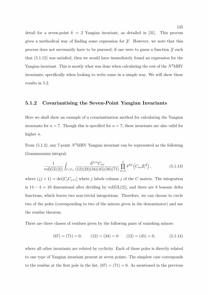
135detail for a seven-point k = 2 Yangian invariant, as detailed in [31]. This process

gives a methodical way of finding some expression for Y. However, we note that this

process does not necessarily have to be pursued; if one were to guess a function Y such

that (5.1.12) was satisfied, then we would have immediately found an expression for the

Yangian invariant. This is mostly what was done when calculating the rest of the N2MHV

invariants; specifically when looking to write some in a simple way. We will show these

results in 5.2.

5.1.2 Covariantising the Seven-Point Yangian Invariants

Here we shall show an example of a covariantisation method for calculating the Yangian

invariants for n = 7. Though this is specified for n = 7, these invariants are also valid for

higher n.

From (5.1.2), any 7-point N2MHV Yangian invariant can be represented as the following

Grassmannian integral:

1vol[GL(2)]

∫C⊂Γσ

d2×nCαi(12)(23)(34)(45)(56)(71)

2∏α=1

δ4|4(CαiZAi

), (5.1.13)

where (jj + 1) = det[CjCj+1] where j labels column j of the C matrix. The integration

is 14 − 4 = 10 dimensional after dividing by vol[GL(2)], and there are 8 bosonic delta

functions, which leaves two non-trivial integrations. Therefore, we can choose to circle

two of the poles (corresponding to two of the minors given in the denominator) and use

the residue theorem.

There are three classes of residues given by the following pairs of vanishing minors

(67) = (71) = 0, (12) = (34) = 0 (12) = (45) = 0, (5.1.14)

where all other invariants are related by cyclicity. Each of these poles is directly related

to one type of Yangian invariant present at seven points. The simplest case corresponds

to the residue at the first pole in the list, (67) = (71) = 0. As mentioned in the previous

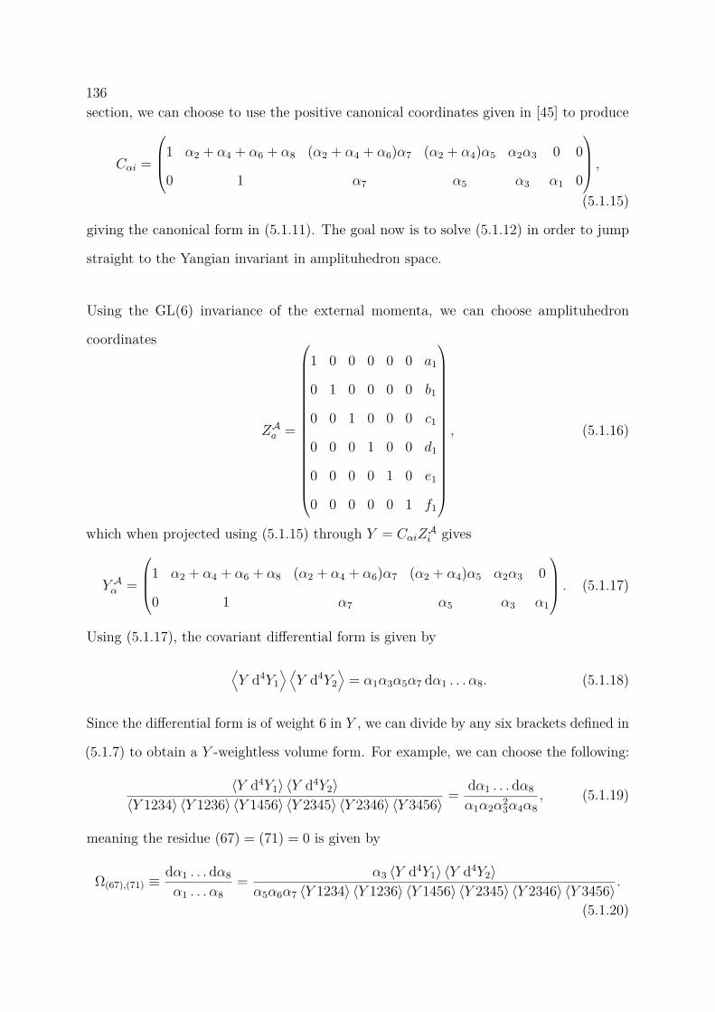
136section, we can choose to use the positive canonical coordinates given in [45] to produce

Cαi =

1 α2 + α4 + α6 + α8 (α2 + α4 + α6)α7 (α2 + α4)α5 α2α3 0 0

0 1 α7 α5 α3 α1 0

,(5.1.15)

giving the canonical form in (5.1.11). The goal now is to solve (5.1.12) in order to jump

straight to the Yangian invariant in amplituhedron space.

Using the GL(6) invariance of the external momenta, we can choose amplituhedron

coordinates

ZAa =

1 0 0 0 0 0 a1

0 1 0 0 0 0 b1

0 0 1 0 0 0 c1

0 0 0 1 0 0 d1

0 0 0 0 1 0 e1

0 0 0 0 0 1 f1

, (5.1.16)

which when projected using (5.1.15) through Y = CαiZAi gives

Y Aα =

1 α2 + α4 + α6 + α8 (α2 + α4 + α6)α7 (α2 + α4)α5 α2α3 0

0 1 α7 α5 α3 α1

. (5.1.17)

Using (5.1.17), the covariant differential form is given by

⟨Y d4Y1

⟩ ⟨Y d4Y2

⟩= α1α3α5α7 dα1 . . . α8. (5.1.18)

Since the differential form is of weight 6 in Y , we can divide by any six brackets defined in

(5.1.7) to obtain a Y -weightless volume form. For example, we can choose the following:

〈Y d4Y1〉 〈Y d4Y2〉〈Y 1234〉 〈Y 1236〉 〈Y 1456〉 〈Y 2345〉 〈Y 2346〉 〈Y 3456〉 = dα1 . . . dα8

α1α2α23α4α8

, (5.1.19)

meaning the residue (67) = (71) = 0 is given by

Ω(67),(71) ≡dα1 . . . dα8

α1 . . . α8= α3 〈Y d4Y1〉 〈Y d4Y2〉α5α6α7 〈Y 1234〉 〈Y 1236〉 〈Y 1456〉 〈Y 2345〉 〈Y 2346〉 〈Y 3456〉 .

(5.1.20)

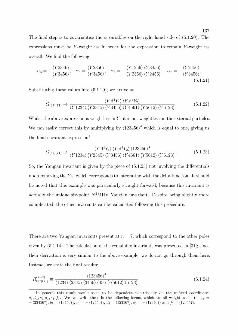
137The final step is to covariantise the α variables on the right hand side of (5.1.20). The

expressions must be Y -weightless in order for the expression to remain Y -weightless

overall. We find the following:

α3 = −〈Y 2346〉〈Y 3456〉 , α5 = 〈Y 2356〉

〈Y 3456〉 , α6 = −〈Y 1256〉 〈Y 3456〉〈Y 2356〉 〈Y 2456〉 , α7 = −〈Y 2456〉

〈Y 3456〉 .

(5.1.21)

Substituting these values into (5.1.20), we arrive at

Ω(67)(71) →〈Y d4Y1〉 〈Y d4Y2〉

〈Y 1234〉 〈Y 2345〉 〈Y 3456〉 〈Y 4561〉 〈Y 5612〉 〈Y 6123〉 . (5.1.22)

Whilst the above expression is weightless in Y , it is not weightless on the external particles.

We can easily correct this by multiplying by 〈123456〉4 which is equal to one, giving us

the final covariant expression1

Ω(67)(71) →〈Y d4Y1〉 〈Y d4Y2〉 〈123456〉4

〈Y 1234〉 〈Y 2345〉 〈Y 3456〉 〈Y 4561〉 〈Y 5612〉 〈Y 6123〉 . (5.1.23)

So, the Yangian invariant is given by the piece of (5.1.23) not involving the differentials

upon removing the Y s, which corresponds to integrating with the delta function. It should

be noted that this example was particularly straight forward, because this invariant is

actually the unique six-point N2MHV Yangian invariant. Despite being slightly more

complicated, the other invariants can be calculated following this procedure.

There are two Yangian invariants present at n = 7, which correspond to the other poles

given by (5.1.14). The calculation of the remaining invariants was presented in [31]; since

their derivation is very similar to the above example, we do not go through them here.

Instead, we state the final results:

R(k=2)(67)(71) ≡

〈123456〉4

〈1234〉 〈2345〉 〈3456〉 〈4561〉 〈5612〉 〈6123〉 , (5.1.24)

1In general this result would seem to be dependent non-trivially on the unfixed coordinatesa1, b1, c1, d1, e1, f1. We can write these in the following forms, which are all weightless in Y : a1 =−〈234567〉, b1 = 〈134567〉, c1 = −〈124567〉, d1 = 〈123567〉, e1 = −〈123467〉 and f1 = 〈123457〉.

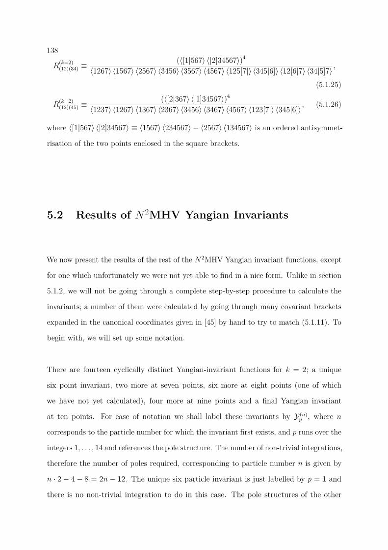
138

R(k=2)(12)(34) ≡

(〈[1|567〉 〈|2]34567〉)4

〈1267〉 〈1567〉 〈2567〉 〈3456〉 〈3567〉 〈4567〉 〈125[7|〉 〈345|6]〉 〈12[6|7〉 〈34|5]7〉 ,

(5.1.25)

R(k=2)(12)(45) ≡

(〈[2|367〉 〈|1]34567〉)4

〈1237〉 〈1267〉 〈1367〉 〈2367〉 〈3456〉 〈3467〉 〈4567〉 〈123[7|〉 〈345|6]〉 , (5.1.26)

where 〈[1|567〉 〈|2]34567〉 ≡ 〈1567〉 〈234567〉 − 〈2567〉 〈134567〉 is an ordered antisymmet-

risation of the two points enclosed in the square brackets.

5.2 Results of N 2MHV Yangian Invariants

We now present the results of the rest of the N2MHV Yangian invariant functions, except

for one which unfortunately we were not yet able to find in a nice form. Unlike in section

5.1.2, we will not be going through a complete step-by-step procedure to calculate the

invariants; a number of them were calculated by going through many covariant brackets

expanded in the canonical coordinates given in [45] by hand to try to match (5.1.11). To

begin with, we will set up some notation.

There are fourteen cyclically distinct Yangian-invariant functions for k = 2; a unique

six point invariant, two more at seven points, six more at eight points (one of which

we have not yet calculated), four more at nine points and a final Yangian invariant

at ten points. For ease of notation we shall label these invariants by Y(n)p , where n

corresponds to the particle number for which the invariant first exists, and p runs over the

integers 1, . . . , 14 and references the pole structure. The number of non-trivial integrations,

therefore the number of poles required, corresponding to particle number n is given by

n · 2 − 4 − 8 = 2n − 12. The unique six particle invariant is just labelled by p = 1 and

there is no non-trivial integration to do in this case. The pole structures of the other

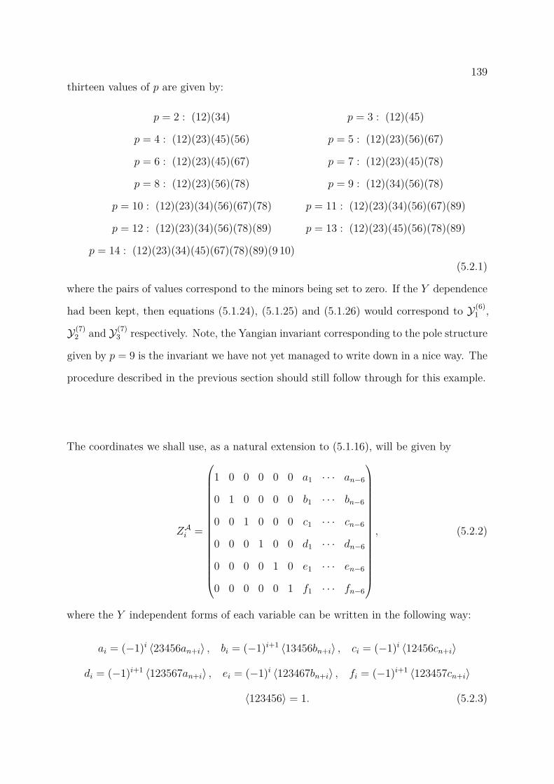
139thirteen values of p are given by:

p = 2 : (12)(34) p = 3 : (12)(45)

p = 4 : (12)(23)(45)(56) p = 5 : (12)(23)(56)(67)

p = 6 : (12)(23)(45)(67) p = 7 : (12)(23)(45)(78)

p = 8 : (12)(23)(56)(78) p = 9 : (12)(34)(56)(78)

p = 10 : (12)(23)(34)(56)(67)(78) p = 11 : (12)(23)(34)(56)(67)(89)

p = 12 : (12)(23)(34)(56)(78)(89) p = 13 : (12)(23)(45)(56)(78)(89)

p = 14 : (12)(23)(34)(45)(67)(78)(89)(9 10)(5.2.1)

where the pairs of values correspond to the minors being set to zero. If the Y dependence

had been kept, then equations (5.1.24), (5.1.25) and (5.1.26) would correspond to Y(6)1 ,

Y(7)2 and Y(7)

3 respectively. Note, the Yangian invariant corresponding to the pole structure

given by p = 9 is the invariant we have not yet managed to write down in a nice way. The

procedure described in the previous section should still follow through for this example.

The coordinates we shall use, as a natural extension to (5.1.16), will be given by

ZAi =

1 0 0 0 0 0 a1 · · · an−6

0 1 0 0 0 0 b1 · · · bn−6

0 0 1 0 0 0 c1 · · · cn−6

0 0 0 1 0 0 d1 · · · dn−6

0 0 0 0 1 0 e1 · · · en−6

0 0 0 0 0 1 f1 · · · fn−6

, (5.2.2)

where the Y independent forms of each variable can be written in the following way:

ai = (−1)i 〈23456an+i〉 , bi = (−1)i+1 〈13456bn+i〉 , ci = (−1)i 〈12456cn+i〉

di = (−1)i+1 〈123567an+i〉 , ei = (−1)i 〈123467bn+i〉 , fi = (−1)i+1 〈123457cn+i〉

〈123456〉 = 1. (5.2.3)

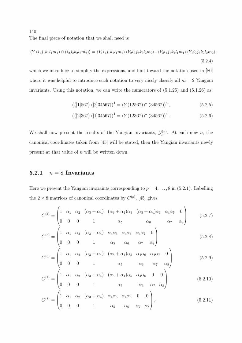
140The final piece of notation that we shall need is

〈Y (i1j1k1l1m1) ∩ (i2j2k2l2m2)〉 = 〈Y1i1j1k1l1m1〉 〈Y2i2j2k2l2m2〉−〈Y2i1j1k1l1m1〉 〈Y1i2j2k2l2m2〉 ,

(5.2.4)

which we introduce to simplify the expressions, and hint toward the notation used in [80]

where it was helpful to introduce such notation to very nicely classify all m = 2 Yangian

invariants. Using this notation, we can write the numerators of (5.1.25) and (5.1.26) as:

(〈[1|567〉 〈|2]34567〉)4 = 〈Y (12567) ∩ (34567)〉4 , (5.2.5)

(〈[2|367〉 〈|1]34567〉)4 = 〈Y (12367) ∩ (34567)〉4 . (5.2.6)

We shall now present the results of the Yangian invariants, Y(n)p . At each new n, the

canonical coordinates taken from [45] will be stated, then the Yangian invariants newly

present at that value of n will be written down.

5.2.1 n = 8 Invariants

Here we present the Yangian invaraints corresponding to p = 4, . . . , 8 in (5.2.1). Labelling

the 2× 8 matrices of canonical coordinates by C(p), [45] gives

C(4) =

1 α1 α2 (α3 + α4) (α3 + α4)α5 (α3 + α4)α6 α4α7 0

0 0 0 1 α5 α6 α7 α8

(5.2.7)

C(5) =

1 α1 α2 (α3 + α4) α4α5 α4α6 α4α7 0

0 0 0 1 α5 α6 α7 α8

(5.2.8)

C(6) =

1 α1 α2 (α3 + α4) (α3 + α4)α5 α4α6 α4α7 0

0 0 0 1 α5 α6 α7 α8

(5.2.9)

C(7) =

1 α1 α2 (α3 + α4) (α3 + α4)α5 α4α6 0 0

0 0 0 1 α5 α6 α7 α8

(5.2.10)

C(8) =

1 α1 α2 (α3 + α4) α4α5 α4α6 0 0

0 0 0 1 α5 α6 α7 α8

, (5.2.11)

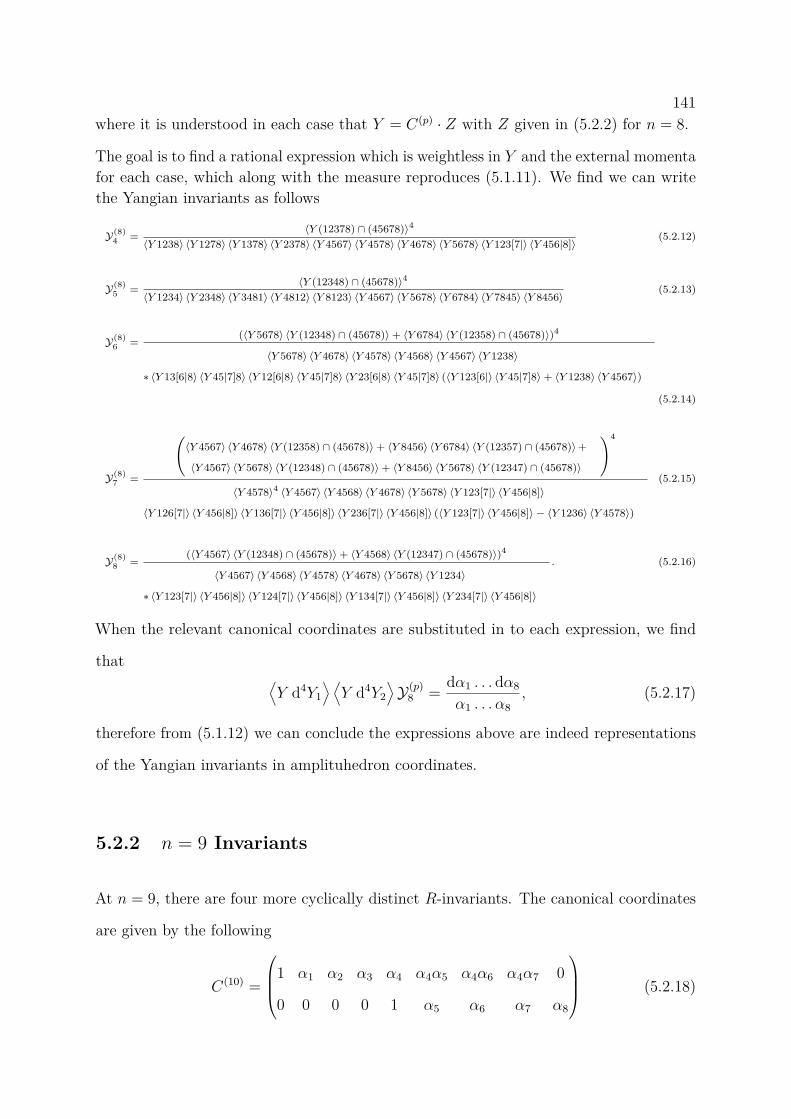
141where it is understood in each case that Y = C(p) · Z with Z given in (5.2.2) for n = 8.

The goal is to find a rational expression which is weightless in Y and the external momentafor each case, which along with the measure reproduces (5.1.11). We find we can writethe Yangian invariants as follows

Y(8)4 =

〈Y (12378) ∩ (45678)〉4

〈Y 1238〉 〈Y 1278〉 〈Y 1378〉 〈Y 2378〉 〈Y 4567〉 〈Y 4578〉 〈Y 4678〉 〈Y 5678〉 〈Y 123[7|〉 〈Y 456|8]〉(5.2.12)

Y(8)5 =

〈Y (12348) ∩ (45678)〉4

〈Y 1234〉 〈Y 2348〉 〈Y 3481〉 〈Y 4812〉 〈Y 8123〉 〈Y 4567〉 〈Y 5678〉 〈Y 6784〉 〈Y 7845〉 〈Y 8456〉(5.2.13)

Y(8)6 =

(〈Y 5678〉 〈Y (12348) ∩ (45678)〉+ 〈Y 6784〉 〈Y (12358) ∩ (45678)〉)4

〈Y 5678〉 〈Y 4678〉 〈Y 4578〉 〈Y 4568〉 〈Y 4567〉 〈Y 1238〉

∗ 〈Y 13[6|8〉 〈Y 45|7]8〉 〈Y 12[6|8〉 〈Y 45|7]8〉 〈Y 23[6|8〉 〈Y 45|7]8〉 (〈Y 123[6|〉 〈Y 45|7]8〉+ 〈Y 1238〉 〈Y 4567〉)

(5.2.14)

Y(8)7 =

(〈Y 4567〉 〈Y 4678〉 〈Y (12358) ∩ (45678)〉+ 〈Y 8456〉 〈Y 6784〉 〈Y (12357) ∩ (45678)〉+

〈Y 4567〉 〈Y 5678〉 〈Y (12348) ∩ (45678)〉+ 〈Y 8456〉 〈Y 5678〉 〈Y (12347) ∩ (45678)〉

)4

〈Y 4578〉4 〈Y 4567〉 〈Y 4568〉 〈Y 4678〉 〈Y 5678〉 〈Y 123[7|〉 〈Y 456|8]〉

〈Y 126[7|〉 〈Y 456|8]〉 〈Y 136[7|〉 〈Y 456|8]〉 〈Y 236[7|〉 〈Y 456|8]〉 (〈Y 123[7|〉 〈Y 456|8]〉 − 〈Y 1236〉 〈Y 4578〉)

(5.2.15)

Y(8)8 =

(〈Y 4567〉 〈Y (12348) ∩ (45678)〉+ 〈Y 4568〉 〈Y (12347) ∩ (45678)〉)4

〈Y 4567〉 〈Y 4568〉 〈Y 4578〉 〈Y 4678〉 〈Y 5678〉 〈Y 1234〉

∗ 〈Y 123[7|〉 〈Y 456|8]〉 〈Y 124[7|〉 〈Y 456|8]〉 〈Y 134[7|〉 〈Y 456|8]〉 〈Y 234[7|〉 〈Y 456|8]〉

. (5.2.16)

When the relevant canonical coordinates are substituted in to each expression, we find

that ⟨Y d4Y1

⟩ ⟨Y d4Y2

⟩Y(p)

8 = dα1 . . . dα8

α1 . . . α8, (5.2.17)

therefore from (5.1.12) we can conclude the expressions above are indeed representations

of the Yangian invariants in amplituhedron coordinates.

5.2.2 n = 9 Invariants

At n = 9, there are four more cyclically distinct R-invariants. The canonical coordinates

are given by the following

C(10) =

1 α1 α2 α3 α4 α4α5 α4α6 α4α7 0

0 0 0 0 1 α5 α6 α7 α8

(5.2.18)

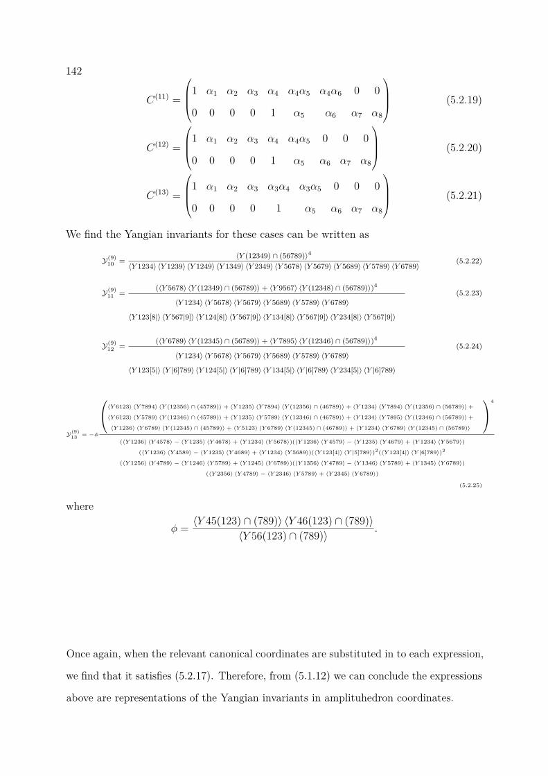
142

C(11) =

1 α1 α2 α3 α4 α4α5 α4α6 0 0

0 0 0 0 1 α5 α6 α7 α8

(5.2.19)

C(12) =

1 α1 α2 α3 α4 α4α5 0 0 0

0 0 0 0 1 α5 α6 α7 α8

(5.2.20)

C(13) =

1 α1 α2 α3 α3α4 α3α5 0 0 0

0 0 0 0 1 α5 α6 α7 α8

(5.2.21)

We find the Yangian invariants for these cases can be written as

Y(9)10 =

〈Y (12349) ∩ (56789)〉4

〈Y 1234〉 〈Y 1239〉 〈Y 1249〉 〈Y 1349〉 〈Y 2349〉 〈Y 5678〉 〈Y 5679〉 〈Y 5689〉 〈Y 5789〉 〈Y 6789〉(5.2.22)

Y(9)11 =

(〈Y 5678〉 〈Y (12349) ∩ (56789)〉+ 〈Y 9567〉 〈Y (12348) ∩ (56789)〉)4

〈Y 1234〉 〈Y 5678〉 〈Y 5679〉 〈Y 5689〉 〈Y 5789〉 〈Y 6789〉

〈Y 123[8|〉 〈Y 567|9]〉 〈Y 124[8|〉 〈Y 567|9]〉 〈Y 134[8|〉 〈Y 567|9]〉 〈Y 234[8|〉 〈Y 567|9]〉

(5.2.23)

Y(9)12 =

(〈Y 6789〉 〈Y (12345) ∩ (56789)〉+ 〈Y 7895〉 〈Y (12346) ∩ (56789)〉)4

〈Y 1234〉 〈Y 5678〉 〈Y 5679〉 〈Y 5689〉 〈Y 5789〉 〈Y 6789〉

〈Y 123[5|〉 〈Y |6]789〉 〈Y 124[5|〉 〈Y |6]789〉 〈Y 134[5|〉 〈Y |6]789〉 〈Y 234[5|〉 〈Y |6]789〉

(5.2.24)

Y(9)13 = −φ

〈Y 6123〉 〈Y 7894〉 〈Y (12356) ∩ (45789)〉 + 〈Y 1235〉 〈Y 7894〉 〈Y (12356) ∩ (46789)〉 + 〈Y 1234〉 〈Y 7894〉 〈Y (12356) ∩ (56789)〉+

〈Y 6123〉 〈Y 5789〉 〈Y (12346) ∩ (45789)〉 + 〈Y 1235〉 〈Y 5789〉 〈Y (12346) ∩ (46789)〉 + 〈Y 1234〉 〈Y 7895〉 〈Y (12346) ∩ (56789)〉+

〈Y 1236〉 〈Y 6789〉 〈Y (12345) ∩ (45789)〉 + 〈Y 5123〉 〈Y 6789〉 〈Y (12345) ∩ (46789)〉 + 〈Y 1234〉 〈Y 6789〉 〈Y (12345) ∩ (56789)〉

4

(〈Y 1236〉 〈Y 4578〉 − 〈Y 1235〉 〈Y 4678〉 + 〈Y 1234〉 〈Y 5678〉)(〈Y 1236〉 〈Y 4579〉 − 〈Y 1235〉 〈Y 4679〉 + 〈Y 1234〉 〈Y 5679〉)

(〈Y 1236〉 〈Y 4589〉 − 〈Y 1235〉 〈Y 4689〉 + 〈Y 1234〉 〈Y 5689〉)(〈Y 123[4|〉 〈Y |5]789〉)2(〈Y 123[4|〉 〈Y |6]789〉)2

(〈Y 1256〉 〈Y 4789〉 − 〈Y 1246〉 〈Y 5789〉 + 〈Y 1245〉 〈Y 6789〉)(〈Y 1356〉 〈Y 4789〉 − 〈Y 1346〉 〈Y 5789〉 + 〈Y 1345〉 〈Y 6789〉)

(〈Y 2356〉 〈Y 4789〉 − 〈Y 2346〉 〈Y 5789〉 + 〈Y 2345〉 〈Y 6789〉)

(5.2.25)

where

φ = 〈Y 45(123) ∩ (789)〉 〈Y 46(123) ∩ (789)〉〈Y 56(123) ∩ (789)〉 .

Once again, when the relevant canonical coordinates are substituted in to each expression,

we find that it satisfies (5.2.17). Therefore, from (5.1.12) we can conclude the expressions

above are representations of the Yangian invariants in amplituhedron coordinates.

1435.2.3 n = 10 Invariants

There is one final Yangian invariant present at ten points and beyond. The canonical

coordinates for this term are given by

C(14) =

1 α1 α2 α3 α4 0 0 0 0 0

0 0 0 0 0 1 α5 α6 α7 α8

, (5.2.26)

with Y = C(14) · Z. The corresponding Yangian invariant is given by

〈Y (12345) ∩ (6789(10))〉4

〈Y 1234〉 〈Y 1235〉 〈Y 1245〉 〈Y 1345〉 〈Y 2345〉 〈Y 6789〉 〈Y 679(10)〉 〈Y 689(10)〉 〈Y 789(10)〉 〈Y 678(10)〉

(5.2.27)

5.3 Concluding Remarks

In this chapter, we have presented expressions for most of the N2MHV Yangian invariants

for N = 4 SYM in amplituhedron coordinates. There are a number of advantages in

writing the invariants in amplituhedron coordinates over the original coordinates. For

example, non-trivial identities which are very hard to see in the superspace formalism

arise naturally as Schouten-like identities in the bosonised quantities.

By writing the m = 2 Yangian invariants in (m = 2) amplituhedron coordinates, it was

shown that the n-point NkMHV Yangian invariants can be classified by labelling them

as a general configuration of k non-intersecting triangles in an n sided polygon. One

would hope that there may be a way to generalise this classification to m = 4 Yangian

invariants, or at least use an uplifted version of this construction to describe some subset

of the invariants. We already see that some of the N2MHV invariants have very simple

forms; see for example (5.1.25), (5.1.26) with numerators written in the form given in

(5.2.5), as well as (5.2.12), (5.2.22) and (5.2.27). It would be interesting to investigate

why these forms are particularly simple, and see if they can be generalised to a subset

of invariants with k > 2. It would also be interesting to see if the invariants with more

complicated expressions can be written in a simpler way, and further, see if all k = 2

invariants can be classified in a simple geometric way that can be extended to k > 2.

144Moreover, these Yangian invariants can be used to continue the work of [31]. There,

the authors managed to extract individual amplitudes from the four-point correlator by

assuming Yangian symmetry and an appropriate basis of planar dual conformal integrands.

Writing the R invariants in amplituhedron coordinates was a necessary ingredient of the

method which they tested up to seven points and two loops. In order to move to higher

points, the n = 8 invariants are required; it would be beneficial to first find a way to write

Y(8)9 in as simple a way as possible.

Chapter 6

Conclusion

To conclude, let us briefly review the main results of each chapter, and indicate some

directions in which the research could be continued.

In this thesis, we have continued the exploration of three fundamental objects in four

dimensional planar supersymmetric Yang-Mills theory; amplitudes, operators and invari-

ants.

In chapter 3, we utilised the Wilson loop / amplitude duality in the hopes of finding a very

explicit tesselation of the amplituhedron using Wilson loop diagrams (WLDs). The WLDs

split the amplitude into well defined pieces as a sum of planar Feynman diagrams and

whilst each individual expression contains spurious poles, they all cancel when summed

leaving only the physical poles of the amplitude. Motivated by this property, and the fact

that each diagram could be naturally associated with a canonical form of a geometrical

object in the same subspace as the amplituhedron, Gr(k, k + 4), we set out to explore

whether the geometrical regions given by each diagram could be glued together to give

a final “good geometry” i.e. one with no spurious boundaries left unmatched (locally)

pairwise. Whilst this was possible for the NMHV case, we proved that it is not possible

for N2MHV and beyond. The principle of the proof can be very nicely summed up by

Figure 6.1.

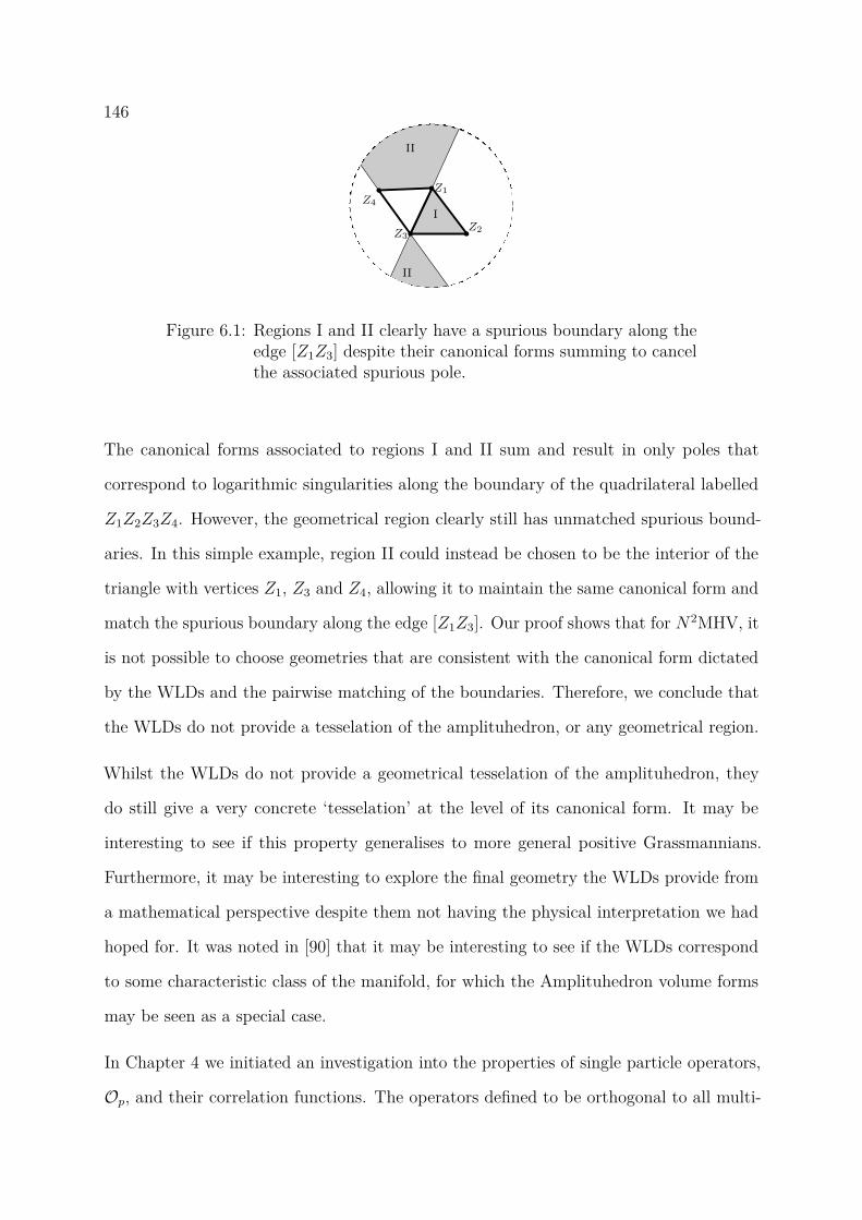
146

I

II

II

Z1

Z2Z3

Z4

Figure 6.1: Regions I and II clearly have a spurious boundary along theedge [Z1Z3] despite their canonical forms summing to cancelthe associated spurious pole.

The canonical forms associated to regions I and II sum and result in only poles that

correspond to logarithmic singularities along the boundary of the quadrilateral labelled

Z1Z2Z3Z4. However, the geometrical region clearly still has unmatched spurious bound-

aries. In this simple example, region II could instead be chosen to be the interior of the

triangle with vertices Z1, Z3 and Z4, allowing it to maintain the same canonical form and

match the spurious boundary along the edge [Z1Z3]. Our proof shows that for N2MHV, it

is not possible to choose geometries that are consistent with the canonical form dictated

by the WLDs and the pairwise matching of the boundaries. Therefore, we conclude that

the WLDs do not provide a tesselation of the amplituhedron, or any geometrical region.

Whilst the WLDs do not provide a geometrical tesselation of the amplituhedron, they

do still give a very concrete ‘tesselation’ at the level of its canonical form. It may be

interesting to see if this property generalises to more general positive Grassmannians.

Furthermore, it may be interesting to explore the final geometry the WLDs provide from

a mathematical perspective despite them not having the physical interpretation we had

hoped for. It was noted in [90] that it may be interesting to see if the WLDs correspond

to some characteristic class of the manifold, for which the Amplituhedron volume forms

may be seen as a special case.

In Chapter 4 we initiated an investigation into the properties of single particle operators,

Op, and their correlation functions. The operators defined to be orthogonal to all multi-

147trace operators, and are appropriate for describing single-particle states of superstring

theory on AdS5 × S5. We found explicit formulae for them in three different bases:

the trace basis, the basis corresponding to the eigenvalues of the operators and in the

Schur polynomial basis. Furthermore, we found an explicit expression for their two point

function, and show that for weight greater than one the U(N) SPOs are simply the SU(N)

SPOs, or more precisely in substituting ψ = φ− TrφN

we have

OU(N)p [φ] = OSU(N)

p [ψ] p ≥ 2.

We made contact with the gravity side, and pointed out that in the large N limit, as

the length of the operator increases the single-particle operator naturally interpolates

between the single-trace and the sphere giant graviton.

The extension of single particle operators to a full basis of half-BPS operators was then

discussed by simply taking products of the operators; we referred to these as multi-particle

operators. This new basis has the advantage of being valid in U(N) and SU(N) gauge

theories (by either allowing O1 contributions in the product or not respectively), and

naturally cuts off when the length of any of the single-particle operators exceeds the

number of colours.

We then went on to study correlators of single particle operators, beginning with a very

interesting theorem regarding multipoint orthogonality:

Multipoint Orthogonality Theorem. Consider any diagram contributing to a half-

BPS correlator that has a single particle operator Op connected to two sub-diagrams,

with the sub-diagrams themselves disconnected from each other. Any propagator structure

consistent with this type of diagram has a vanishing colour factor. This statement holds

for both U(N) and SU(N) free theories.

This theorem meant that a huge number of diagrams thought to contribute to various

correlators of SPOs were actually zero, simplifying a number of calculations that followed.

In particular, an important corollary of this theorem was the following:

148Near-Extremal Correlators Vanish. Any near-extremal SU(N) correlator in free

theory, where the largest charge operator is a single-particle operator, vanishes, i.e.

〈Op(x)Tq1(x1) . . . Tqn−1(xn−1)〉 = 0 k ≤ n− 3 . (6.0.1)

In the U(N) theory, a similar statement can be made but with the caveat that it is true

only for connected correlators.

Using the above results, we were able to calculate expressions for all maximally and next-

to-maximally extremal free correlators, and were able to calculate explicit expressions for

some multi-particle two and three point functions.

There are a number of ways in which this topic can be further explored. Firstly, there are

still a large number of things left to calculate even in the free theory. For example, the

simple nature of the end formula for lowering extremality three-point functions hints that

there may be a way to write a general formula for all Nk maximally extremal three-point

functions. As mentioned previously, the multi-particle basis is not orthogonal; it would

be interesting to see if a canonical way of orthogonalising the single particle operators

could be discovered, perhaps by exploring the string theory point of view further.

One could try to generalise the story of single particle operators described here to beyond

the half-BPS sector. Bases do exist already for more general operators beyond the half-

BPS sector [149–155], but it would be interesting to revisit these from the perspective of

the single-particle operators.

In a slightly different direction, one would assume that the definition of the single particle

operator holds beyond the U(N) and SU(N) gauge theories, to the orthogonal and

symplectic gauge groups in N = 4 SYM. These can be obtained via a Z2 orientifold

projection of the standard AdS5 × S5 set-up [156]. There have been studies on half-BPS

operators in these theories [157–160], so it would be useful to consider single particle

operators in these gauge theories and see how they compare to those operators already

studied. It would also be interesting to study single particle states for other backgrounds,

149for example AdS3 [161], ABJM, and for the slightly mysterious six-dimensional (2, 0)

theory on AdS7 × S4.

Finally, it would be interesting to consider aspects of the dynamics of the single-particle

operators that have not yet been explored, and go beyond the computation of the one-loop

amplitudes in [115], along the lines suggested in [162]. The trace basis is widely used

in the context of integrability, and in turn integrability based techniques have allowed

the computation of exact correlators (see work on the octagon configuration in [163–167]

and the five-point analogue called the decagon configuration in [168]). It would be very

interesting to understand how the integrability based techniques [169, 170] modify or

adapt when correlators of single particle operators are considered.

Finally, in Chapter 6 we looked to write all the N2MHV Yangian invariants of N = 4

SYM in amplituhedron coordinates. We began be describing a covariantisation algorithm

detailed in [31] that made this possible. Then we presented results for all bar one of the

14 N2MHV Yangian invaraints. It was evident that some had particular simple forms; it

would be interesting to see if there exists a nice geometrical way of classifying (a subset of)

Yangian invariants for all k > 2, in a similar way that was done for all m = 2 invariants

in [80].

Appendix A

Spurious Pole Cancellation for

Special N2MHV Three-Way Case

Here, we show how the algebraic cancellation works for the special three-way cancellation

illustrated in Figure 3.8 and the surrounding discussion:

Figure A.1: The WLDs corresponding to the special three way cancella-tion, with the limits of the residues illustrated by the arrowson each WLD.

To begin, the three integrals given by the WLDs in Figure A.1 are

I(D′1) =∫ da1 db1 dc1 dd1 de1 df1 dg1 dh1

a1b1g1h1e1(c1f1 − d1e1)d1δ(8|8) (C ′1 · Z) (A.0.1)

I(D′2) =∫ da2 db2 dc2 dd2 de2 df2 dg2 dh2

c2d2g2h2a2(e2b2 − a2f2)f2δ(8|8) (C ′2 · Z) (A.0.2)

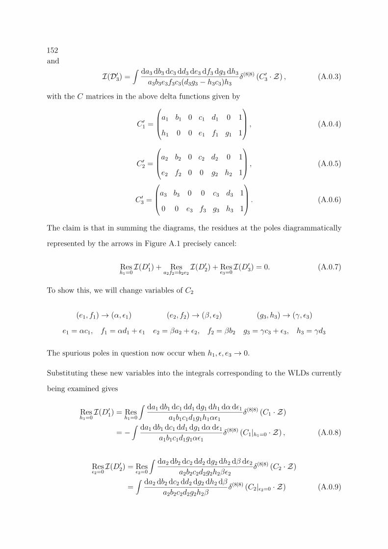
152and

I(D′3) =∫ da3 db3 dc3 dd3 de3 df3 dg3 dh3

a3b3e3f3c3(d3g3 − h3c3)h3δ(8|8) (C ′3 · Z) , (A.0.3)

with the C matrices in the above delta functions given by

C ′1 =

a1 b1 0 c1 d1 0 1

h1 0 0 e1 f1 g1 1

, (A.0.4)

C ′2 =

a2 b2 0 c2 d2 0 1

e2 f2 0 0 g2 h2 1

, (A.0.5)

C ′3 =

a3 b3 0 0 c3 d3 1

0 0 e3 f3 g3 h3 1

. (A.0.6)

The claim is that in summing the diagrams, the residues at the poles diagrammatically

represented by the arrows in Figure A.1 precisely cancel:

Resh1=0I(D′1) + Res

a2f2=b2e2I(D′2) + Res

e3=0I(D′3) = 0. (A.0.7)

To show this, we will change variables of C2

(e1, f1)→ (α, ε1) (e2, f2)→ (β, ε2) (g3, h3)→ (γ, ε3)

e1 = αc1, f1 = αd1 + ε1 e2 = βa2 + ε2, f2 = βb2 g3 = γc3 + ε3, h3 = γd3

The spurious poles in question now occur when h1, ε, e3 → 0.

Substituting these new variables into the integrals corresponding to the WLDs currently

being examined gives

Resh1=0I(D′1) = Res

h1=0

∫ da1 db1 dc1 dd1 dg1 dh1 dα dε1a1b1c1d1g1h1αε1

δ(8|8) (C1 · Z)

= −∫ da1 db1 dc1 dd1 dg1 dα dε1

a1b1c1d1g1αε1δ(8|8) (C1|h1=0 · Z) , (A.0.8)

Resε2=0I(D′2) = Res

ε2=0

∫ da2 db2 dc2 dd2 dg2 dh2 dβ dε2a2b2c2d2g2h2βε2

δ(8|8) (C2 · Z)

=∫ da2 db2 dc2 dd2 dg2 dh2 dβ

a2b2c2d2g2h2βδ(8|8) (C2|ε2=0 · Z) (A.0.9)

153and

Rese3=0I(D′3) = Res

e3=0

∫ da3 db3 dc3 dd3 de3 df3 dγ dε3a3b3c3d3e3f3γε3

δ(8|8) (C3 · Z)

=∫ da3 db3 dc3 dd3 df3 dγ dε3

a3b3c3d3f3γε3δ(8|8) (C3|e3=0 · Z) . (A.0.10)

The measure in each expression is now simply the dlog of all the variables. The associated

C matrices in the delta functions become

C ′1|h1=0 =

a1 b1 0 c1 d1 0 1

0 0 0 αc1 αd1 + ε1 g1 1

, (A.0.11)

C ′2|ε2=0 =

a2 b2 0 c2 d2 0 1

βa2 βb2 0 0 g2 h2 1

, (A.0.12)

C ′3|e3=0 =

a3 b3 0 0 c3 d3 1

0 0 0 f3 γc3 + ε3 γd3 1

. (A.0.13)

In order to compare the three C ′i ∈ GR(2, 7), we must introduce a change of parameteriz-

ation. Utilising the GL(2) invariance, we make the following change of basis for C ′1 and

C ′3,

C ′′1 =

1 0−α1−α

11−α

C ′1 (A.0.14)

and

C ′′3 =

−γ1−γ

11−γ

1 0

C ′3. (A.0.15)

The three matrices C ′′1 , C ′2 and C ′′3 are now of the same form, meaning they have zeros

and ones in the same entries and variables in the others:

C ′′1 =

a1 b1 0 c1 d1 0 1−αa11−α

−αb11−α 0 0 ε1

1−αg1

1−α 1

, (A.0.16)

C ′′3 =

−γa31−γ

−γb31−γ 0 f3

1−γε3

1−γ 0 1

a3 b3 0 0 c3 d3 1

. (A.0.17)

154We make a change of variables for C ′′1 and C ′′3 to the variables of C ′2 as dictated by

matching entries:

C ′′1 :a1 → a2 b1 → b2 c1 → c2

d1 → d2 ε1 → 11−βg2 g1 → 1

1−βh1

α→ −β1− β , (A.0.18)

C ′′3 :a3 → βa2 b3 → βb2 f3 → −βc2

1−β

ε3 → −βd21−β c3 → g2 d3 → h2

γ → 11− β . (A.0.19)

Substituting these new variables into the residues of I (D′1) and I (D′3) and taking the

sum of all three integrals gives

∫ da2 db2 dc2 dd2 dg2 dh2 dβa1b1c1d1g1h1

(− 1β(1− β) + 1

β+ 1

1− β

)δ(8|8) (C ′2 · Z) = 0. (A.0.20)

Therefore, we have shown that (A.0.7) is indeed satisfied.

Appendix B

Character Polynomials

As we saw in section 4.1.2, group theoretic formula for the dual operators to the trace

basis was given by Brown in [127]. This formula was dependent on the character of

any conjugacy class of the symmetric group in any hook representation, where the hook

representations consisted of the representations associated to Young diagrams with one

column and one row. An explicit formula for this set of characters is unknown, however

they are neatly packaged in character polynomials. We give a brief explanation of them

here and show how to calculate the characters given in the character tables in (2.1) using

this technique.1

In [70], the following generating function was defined for the character polynomials for

characters of all hook representations:

∞∑k=0

q1ktk = 1

1 + t

∞∏i=1

(1− (−t)i

)ci. (B.0.1)

Here, q1k is the character polynomial for the hook representation correponding to the

Young diagram with k + 1 boxes in the first column and a row of any length), and ci

denotes the number of cycles of length i the element σ ∈ Sn has.

1We were able to re-write the sum for the single particle operators in terms of other group theoreticquantities described in section 2.4.6, which turned the coefficients of the multi-traces into formulaeexplicit in the weight p and the conjugacy class of the trace structure q1, . . . , qm. So, calculating thesecharacters explicitly did not end up being relevant when continuing to discuss SPOs.

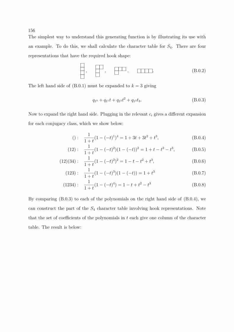
156The simplest way to understand this generating function is by illustrating its use with

an example. To do this, we shall calculate the character table for S4. There are four

representations that have the required hook shape:

, , , . (B.0.2)

The left hand side of (B.0.1) must be expanded to k = 3 giving

q10 + q11t+ q12t2 + q13t3. (B.0.3)

Now to expand the right hand side. Plugging in the relevant ci gives a different expansion

for each conjugacy class, which we show below:

() : 11 + t

(1− (−t)1)4 = 1 + 3t+ 3t2 + t3, (B.0.4)

(12) : 11 + t

(1− (−t)2)(1− (−t))2 = 1 + t− t2 − t3, (B.0.5)

(12)(34) : 11 + t

(1− (−t)2)2 = 1− t− t2 + t3, (B.0.6)

(123) : 11 + t

(1− (−t)3)(1− (−t)) = 1 + t3 (B.0.7)

(1234) : 11 + t

(1− (−t)4) = 1− t+ t2 − t3 (B.0.8)

By comparing (B.0.3) to each of the polynomials on the right hand side of (B.0.4), we

can construct the part of the S4 character table involving hook representations. Note

that the set of coefficients of the polynomials in t each give one column of the character

table. The result is below:

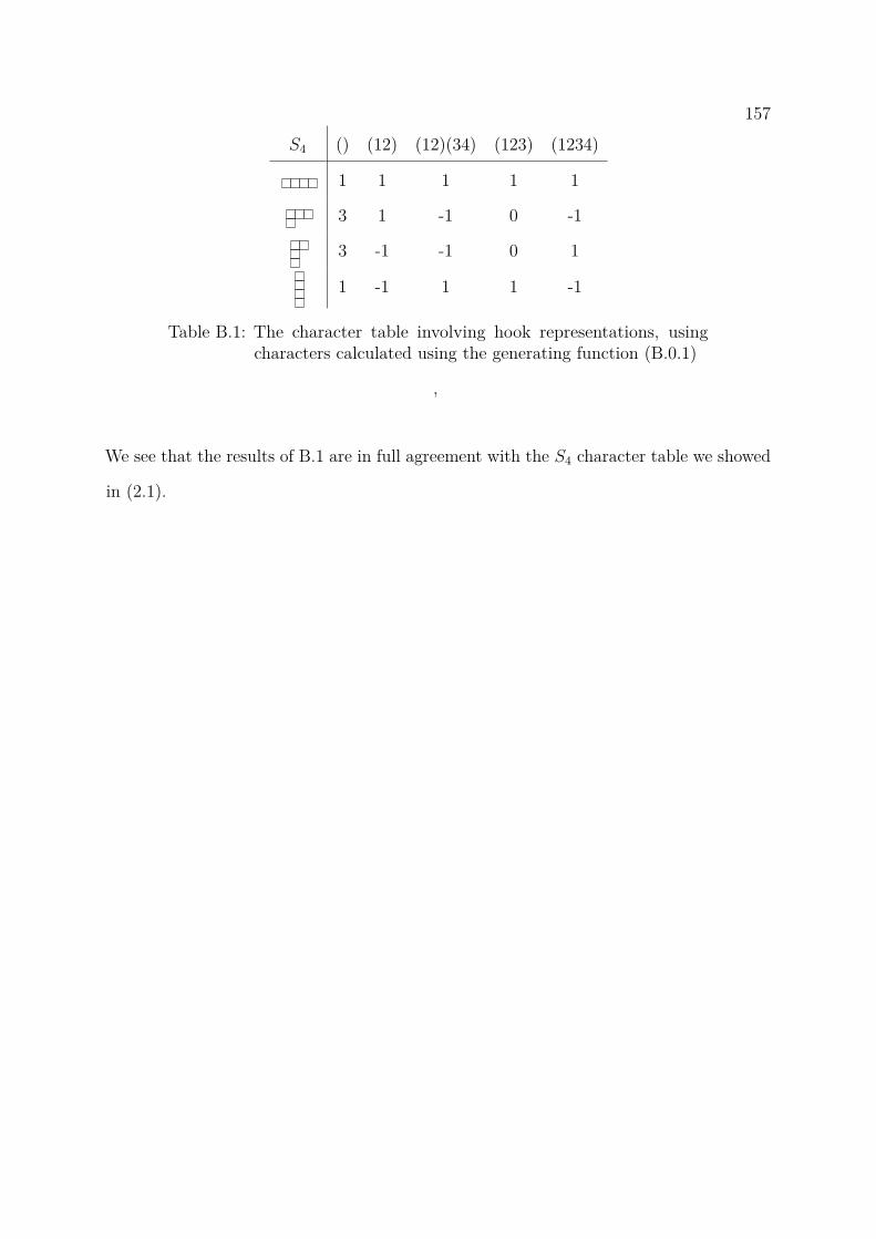
157

S4 () (12) (12)(34) (123) (1234)

1 1 1 1 1

3 1 -1 0 -1

3 -1 -1 0 1

1 -1 1 1 -1

Table B.1: The character table involving hook representations, usingcharacters calculated using the generating function (B.0.1)

,

We see that the results of B.1 are in full agreement with the S4 character table we showed

in (2.1).

Appendix C

Trace Sector Formulae

In section 4.2.2 we obtained the result

Op =∑

q1..qm`pCq1,..,qmTq1,..qm (C.0.1)

Cq1,..qm = |[σq1..qm ]|(p− 1)!

∑s∈P(q1,..,qm)

(−1)|s|+1(N + 1− p)p−Σ(s)(N + p− Σ(s))Σ(s)

(N)p − (N + 1− p)p(C.0.2)

which is explicit in p and q1 . . . qm, and depends on group theory data which we explained

in section 2.4.6.

The value of m distinguishes the splitting of Op into m traces we. We will give explicit

examples for the double trace sector m = 2, and the triple trace sector m = 3.

C.1 Double Trace Sector

Consider the partition q1 + q2 = p. The powerset in the sum is

P (q1q2) = , q1, q2, q1, q2 (C.1.1)

and the corresponding values of Σ are

Σ() = 0 , Σ(q1) = q1 , Σ(q2) = q2 , Σ(q1, q2) = q1 + q2 = p. (C.1.2)

160Furthermore the size of the conjugacy class is |[q1q2]| = p!/(q1q2) as long as q1 6= q2.

Otherwise q1 = q2 = p/2 and |[q1q2]| = p!/(2q1q2) = (p−1)!/(2p). With these informations,

the coefficient of Tq1Tq2 in Op, from (C.0.2), is

Cq1q2 =

p

q1q2× −(N−p+1)p − (N)p + (N−p+1)q2(N+q2)p−q2 + (N−p+1)q1(N+q1)p−q1

(N)p − (N − p+ 1)p2p×−(N−p+1)p − (N)p + 2(N−p+1)p/2(N+p/2)p/2

(N)p − (N − p+ 1)p(C.1.3)

The above formula holds for the coefficients of the double trace contributions to the single

particle operator of any weight.

C.2 Triple Trace Sector

Consider the partition q1 + q2 + q3 = p. By making explicit (C.0.2) we find,

Cq1q2q3 = p

q1q2q3

−(N − p+ 1)p + (N)p(N)p − (N − p+ 1)p

+ (C.2.1)

p

q1q2q3

−∑3i=1(N − p+ 1)qi(N + qi)p−qi +∑3

i=1(N − p+ 1)p−qi(N + p− qi)qi(N)p − (N − p+ 1)p

The other two possible cases, in which qi = qj and q1 = q2 = q3 = p/3, only differ

compared to the result above by the the size of the conjugacy class. In the first case we

have to further divide by 2, and in the second case by 6. This formula thus cover all

possible triple trace contributions to single particle operators of any weight.

For any value of m, i.e. for any trace sector, the function Cq can be made very explicit

in a similar way to the examples above.

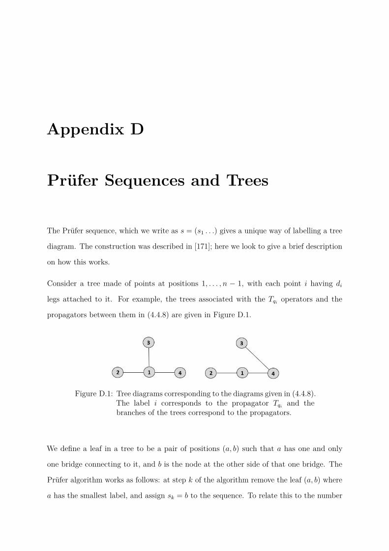
Appendix D

Prüfer Sequences and Trees

The Prüfer sequence, which we write as s = (s1 . . .) gives a unique way of labelling a tree

diagram. The construction was described in [171]; here we look to give a brief description

on how this works.

Consider a tree made of points at positions 1, . . . , n − 1, with each point i having di

legs attached to it. For example, the trees associated with the Tqi operators and the

propagators between them in (4.4.8) are given in Figure D.1.

Figure D.1: Tree diagrams corresponding to the diagrams given in (4.4.8).The label i corresponds to the propagator Tqi and thebranches of the trees correspond to the propagators.

We define a leaf in a tree to be a pair of positions (a, b) such that a has one and only

one bridge connecting to it, and b is the node at the other side of that one bridge. The

Prüfer algorithm works as follows: at step k of the algorithm remove the leaf (a, b) where

a has the smallest label, and assign sk = b to the sequence. To relate this to the number

162of possible Wick contractions for that propagator, write down the contribution

|W(a, b)| = (qa − da + 1)(qb −R(b)), (D.0.1)

where qa, qb corresponds to the charge of the operator at position a, b respectively and

R(b) corresponds to the number of times b has appeared in the sequence previous (i.e.

steps < k). The Prüfer sequence stops when there is only one leaf left, i.e. one pair of

nodes left. However, we do have to write down that final contribution to the number of

Wick contractions given by (D.0.1).

For example, on the left hand side of Figure D.1, the Prüfer algorithm would give the

sequence 1, 1, and the number of Wick contractions at each step would correspond to

|W(2, 1)| = q2q1, |W(3, 1)| = q3(q1 − 1). The total number of wick contractions for

the whole tree though would be the product of the right hand side of each element in

that sequence, multiplied by the result of the final leaf given by |W(3, 1)| = q4(q1 − 2).

Therefore, for this example

|W(T )| = q1q2q3(q1 − 1)(q1 − 2). (D.0.2)

It is very straightforward to continue these considerations to as complicated a tree as you

like.

It is quite evident that the Prüfer Sequence gives a very nice way of ordering Wick

contractions for the purposes of counting the total number of possibilities. It is clear that

the first time two operators i and j appear in the sequence, they count with qiqj, because

necessarily di = 1 or dj = 1. The second time one of this operators appears again, it

counts with qi − 1 or qj − 1, and so on. The total number of Wick contractions is then,

|W [T ]| =n−1∏i=1

qi(qi − 1) . . . (qi − di + 1) (D.0.3)

which is the result we quoted in (4.4.9).

Bibliography

[1] Juan Maldacena. The Large N Limit of Superconformal Field Theories and Super-

gravity. International Journal of Theoretical Physics, 38(4):1113–1133, 1999.

[2] S.S. Gubser, I.R. Klebanov, and A.M. Polyakov. Gauge Theory Correlators from

Non-Critical String Theory. Physics Letters B, 428(1-2):105–114, May 1998.

[3] Edward Witten. Anti-de Sitter Space and Holography. Adv. Theor. Math. Phys.,

2:253–291, 1998.

[4] Ofer Aharony, Steven S. Gubser, Juan Maldacena, Hirosi Ooguri, and Yaron Oz.

Large N Field Theories, String Theory and Gravity. Physics Reports, 323(3-

4):183–386, Jan 2000.

[5] Gerard ’t Hooft. A Planar Diagram Theory for Strong Interactions. Nucl. Phys. B,

72:461, 1974.

[6] Stephen J. Parke and T.R. Taylor. Gluonic Two Goes to Four. Nucl. Phys. B,

269:410–420, 1986.

[7] Stephen J. Parke and T.R. Taylor. An Amplitude for n Gluon Scattering. Phys.

Rev. Lett., 56:2459, 1986.

[8] Zvi Bern, Lance Dixon, David C. Dunbar, and David A. Kosower. One-Loop n-

Point Gauge Theory Amplitudes, Unitarity and Collinear Limits. Nuclear Physics

B, 425(1-2):217–260, Aug 1994.

164[9] Ruth Britto, Freddy Cachazo, and Bo Feng. Generalized Unitarity and One-Loop

Amplitudes in Super-Yang–Mills. Nuclear Physics B, 725(1-2):275–305, Oct 2005.

[10] J.M. Drummond, J. Henn, G.P. Korchemsky, and E. Sokatchev. Generalized Unit-

arity for Super-Amplitudes. Nuclear Physics B, 869(3):452–492, Apr 2013.

[11] Zvi Bern and Yu-tin Huang. Basics of Generalized Unitarity. Journal of Physics

A: Mathematical and Theoretical, 44(45):454003, Oct 2011.

[12] Ruth Britto, Freddy Cachazo, and Bo Feng. New Recursion Relations for Tree

Amplitudes of Gluons. Nuclear Physics B, 715(1-2):499–522, May 2005.

[13] Ruth Britto, Freddy Cachazo, Bo Feng, and Edward Witten. Direct Proof of the

Tree-Level Scattering Amplitude Recursion Relation in Yang-Mills Theory. Physical

Review Letters, 94(18), May 2005.

[14] Freddy Cachazo, Peter Svrcek, and Edward Witten. MHV Vertices And Tree

Amplitudes in Gauge Theory. Journal of High Energy Physics, 2004(09):006–006,

Sep 2004.

[15] James M Drummond, Johannes Henn, Vladimir A Smirnov, and Emery Sokatchev.

Magic Identities for Conformal Four-Point Integrals. Journal of High Energy Physics,

2007(01):064–064, Jan 2007.

[16] J.M. Drummond, J. Henn, G.P. Korchemsky, and E. Sokatchev. Dual Supercon-

formal Symmetry of Scattering Amplitudes in Super Yang–Mills Theory. Nuclear

Physics B, 828(1-2):317–374, Mar 2010.

[17] Andreas Brandhuber, Paul Heslop, and Gabriele Travaglini. Note on Dual Super-

conformal Symmetry of the N = 4 Super Yang-Mills S Matrix. Physical Review D,

78(12), Dec 2008.

165[18] Andreas Brandhuber, Paul Heslop, and Gabriele Travaglini. Proof of the Dual

Conformal Anomaly of One-Loop Amplitudes in N = 4 SYM. Journal of High

Energy Physics, 2009(10):063–063, Oct 2009.

[19] Luis F Alday and Juan Maldacena. Gluon Scattering Amplitudes at Strong Coupling.

Journal of High Energy Physics, 2007(06):064–064, Jun 2007.

[20] J.M. Drummond, G.P. Korchemsky, and E. Sokatchev. Conformal Properties

of Four-Gluon Planar Amplitudes and Wilson Loops. Nuclear Physics B, 795(1-

2):385–408, May 2008.

[21] Andreas Brandhuber, Paul Heslop, and Gabriele Travaglini. MHV Amplitudes in

Super Yang–Mills and Wilson Loops. Nuclear Physics B, 794(1-2):231–243, May

2008.

[22] S. Caron-Huot. Notes on the Scattering Amplitude — Wilson Loop Duality. Journal

of High Energy Physics, 2011(7), Jul 2011.

[23] Lionel Mason and David Skinner. The Complete Planar S-matrix of N = 4 SYM

as a Wilson Loop in Twistor Space. Journal of High Energy Physics, 2010(12), Dec

2010.

[24] A.V. Belitsky, G.P. Korchemsky, and E. Sokatchev. Are Scattering Amplitudes

Dual to Super Wilson Loops? Nuclear Physics B, 855(2):333–360, Feb 2012.

[25] Luis F. Alday, Burkhard Eden, Gregory P. Korchemsky, Juan Maldacena, and

Emery Sokatchev. From Correlation Functions to Wilson Loops. Journal of High

Energy Physics, 2011(9), Sep 2011.

[26] Burkhard Eden, Paul Heslop, Gregory P. Korchemsky, and Emery Sokatchev.

The Super-Correlator/Super-Amplitude Duality: Part I. Nuclear Physics B,

869(3):329–377, Apr 2013.

166[27] Burkhard Eden, Paul Heslop, Gregory P. Korchemsky, and Emery Sokatchev.

The Super-Correlator/Super-Amplitude Duality: Part II. Nuclear Physics B,

869(3):378–416, Apr 2013.

[28] Tim Adamo, Mathew Bullimore, Lionel Mason, and David Skinner. A Proof of the

Correlation Function/Supersymmetric Wilson Loop Correspondence. Journal of

High Energy Physics, 2011(8), Aug 2011.

[29] James Drummond, Johannes Henn, and Jan Plefka. Yangian Symmetry of Scat-

tering Amplitudes in N = 4 Super Yang-Mills Theory. Journal of High Energy

Physics, 2009(05):046–046, May 2009.

[30] Jacob L. Bourjaily, Paul Heslop, and Vuong-Viet Tran. Amplitudes and Correlators

to Ten Loops Using Simple, Graphical Bootstraps. Journal of High Energy Physics,

2016(11), Nov 2016.

[31] Paul Heslop and Vuong-Viet Tran. Multi-Particle Amplitudes from the Four-Point

Correlator in Planar N = 4 SYM. Journal of High Energy Physics, 2018(7), Jul

2018.

[32] Nathan Berkovits and Juan Maldacena. Dual superconformal symmetry, and

the amplitude/Wilson loop connection. Journal of High Energy Physics,

2008(09):062–062, Sep 2008.

[33] Niklas Beisert, Riccardo Ricci, Arkady A. Tseytlin, and Martin Wolf. Dual super-

conformal symmetry from AdS5 × S5 superstring integrability. Physical Review D,

78(12), Dec 2008.

[34] Luis F. Alday and Radu Roiban. Scattering amplitudes, Wilson loops and the

string/gauge theory correspondence. Physics Reports, 468(5):153–211, Nov 2008.

[35] J.M. Drummond, J. Henn, G.P. Korchemsky, and E. Sokatchev. On planar gluon

amplitudes/Wilson loops duality. Nuclear Physics B, 795(1-2):52–68, May 2008.

167[36] J.M. Drummond, J. Henn, G.P. Korchemsky, and E. Sokatchev. Conformal Ward

identities for Wilson loops and a test of the duality with gluon amplitudes. Nuclear

Physics B, 826(1-2):337–364, Feb 2010.

[37] Zvi Bern, Lance J. Dixon, and Vladimir A. Smirnov. Iteration of planar amplitudes

in maximally supersymmetric Yang-Mills theory at three loops and beyond. Physical

Review D, 72(8), Oct 2005.

[38] J.M. Drummond, J. Henn, G.P. Korchemsky, and E. Sokatchev. The hexagon

Wilson loop and the BDS ansatz for the six-gluon amplitude. Physics Letters B,

662(5):456–460, May 2008.

[39] Z. Bern, L. J. Dixon, D. A. Kosower, R. Roiban, M. Spradlin, C. Vergu, and

A. Volovich. Two-loop six-gluon maximally helicity violating amplitude in maximally

supersymmetric Yang-Mills theory. Physical Review D, 78(4), Aug 2008.

[40] J.M. Drummond, J. Henn, G.P. Korchemsky, and E. Sokatchev. Hexagon Wilson

loop = six-gluon MHV amplitude. Nuclear Physics B, 815(1-2):142–173, Jul 2009.

[41] Mathew Bullimore and David Skinner. Holomorphic Linking, Loop Equations and

Scattering Amplitudes in Twistor Space, 2011.

[42] N. Arkani-Hamed, F. Cachazo, C. Cheung, and J. Kaplan. A Duality for the S

Matrix. Journal of High Energy Physics, 2010(3), Mar 2010.

[43] N. Arkani-Hamed, J. Bourjaily, F. Cachazo, and J. Trnka. Local Spacetime Physics

from the Grassmannian. Journal of High Energy Physics, 2011(1), Jan 2011.

[44] N. Arkani-Hamed, J. Bourjaily, F. Cachazo, and J. Trnka. Unification of Residues

and Grassmannian Dualities. Journal of High Energy Physics, 2011(1), Jan 2011.

[45] Nima Arkani-Hamed, Jacob L. Bourjaily, Freddy Cachazo, Alexander B. Goncharov,

Alexander Postnikov, and Jaroslav Trnka. Scattering Amplitudes and the Positive

Grassmannian, 2014.

168[46] Nima Arkani-Hamed, Jacob Bourjaily, Freddy Cachazo, Alexander Goncharov,

Alexander Postnikov, and Jaroslav Trnka. Grassmannian Geometry of Scattering

Amplitudes. Cambridge University Press, 2016.

[47] Nima Arkani-Hamed and Jaroslav Trnka. The Amplituhedron. Journal of High

Energy Physics, 2014(10), Oct 2014.

[48] Nima Arkani-Hamed and Jaroslav Trnka. Into the Amplituhedron. Journal of High

Energy Physics, 2014(12), Dec 2014.

[49] Nima Arkani-Hamed, Cameron Langer, Akshay Yelleshpur Srikant, and Jaroslav

Trnka. Deep Into the Amplituhedron: Amplitude Singularities at All Loops and

Legs. Phys. Rev. Lett., 122:051601, Feb 2019.

[50] Cameron Langer and Akshay Yelleshpur Srikant. All-Loop Cuts from the Amp-

lituhedron. Journal of High Energy Physics, 2019(4), Apr 2019.

[51] I. Prlina, M. Spradlin, J. Stankowicz, and S. Stanojevic. Boundaries of Amplituhedra

and NMHV Symbol Alphabets at Two Loops. Journal of High Energy Physics,

2018(4), Apr 2018.

[52] I. Prlina, M. Spradlin, J. Stankowicz, S. Stanojevic, and A. Volovich. All-Helicity

Symbol Alphabets from Unwound Amplituhedra. Journal of High Energy Physics,

2018(5), May 2018.

[53] T. Dennen, I. Prlina, M. Spradlin, S. Stanojevic, and A. Volovich. Landau Sin-

gularities from the Amplituhedron. Journal of High Energy Physics, 2017(6), Jun

2017.

[54] Lance J. Dixon, Matt von Hippel, Andrew J. McLeod, and Jaroslav Trnka. Multi-

Loop Positivity of the Planar N = 4 SYM Six-Point Amplitude. Journal of High

Energy Physics, 2017(2), Feb 2017.

169[55] Niklas Beisert and Matthias Staudacher. The SYM Integrable Super Spin Chain.

Nuclear Physics B, 670(3):439–463, Oct 2003.

[56] Niklas Beisert, Changrim Ahn, Luis F. Alday, Zoltán Bajnok, James M. Drummond,

Lisa Freyhult, Nikolay Gromov, Romuald A. Janik, Vladimir Kazakov, Thomas

Klose, and et al. Review of AdS/CFT Integrability: An Overview. Letters in

Mathematical Physics, 99(1-3):3–32, Oct 2011.

[57] Paul Heslop and Alastair Stewart. The Twistor Wilson Loop and the Amplituhedron.

Journal of High Energy Physics, 2018(10), Oct 2018.

[58] Francesco Aprile, J. M. Drummond, Paul Heslop, Hyneck Paul, Francesco Sanfil-

ippo, Michele Santagata, and Alastair Stewart. Single Particle Operators and their

Correlators in Free N = 4 SYM. Journal of High Energy Physics, 2020(72), Aug

2020.

[59] Eric D’Hoker and Daniel Z. Freedman. Supersymmetric gauge theories and the

AdS / CFT correspondence. In Theoretical Advanced Study Institute in Elementary

Particle Physics (TASI 2001): Strings, Branes and EXTRA Dimensions, pages

3–158, 1 2002.

[60] V.P. Nair. A Current Algebra for Some Gauge Theory Amplitudes. Phys. Lett. B,

214:215–218, 1988.

[61] Zvi Bern, Lance J. Dixon, David C. Dunbar, and David A. Kosower. Fusing Gauge

Theory Tree Amplitudes into Loop Amplitudes. Nucl. Phys. B, 435:59–101, 1995.

[62] Henriette Elvang and Yu tin Huang. Scattering Amplitudes, 2014.

[63] Andrew Hodges. Eliminating Spurious Poles from Gauge-Theoretic Amplitudes,

2009.

170[64] Lionel Mason and David Skinner. Dual Superconformal Invariance, Momentum

Twistors and Grassmannians. Journal of High Energy Physics, 2009(11):045–045,

Nov 2009.

[65] Dongmin Gang, Yu-tin Huang, Eunkyung Koh, Sangmin Lee, and Arthur E. Lip-

stein. Tree-Level Recursion Relation and Dual Superconformal Symmetry of the

ABJM Theory. Journal of High Energy Physics, 2011(3), Mar 2011.

[66] Yu-tin Huang and Arthur E. Lipstein. Dual Superconformal Symmetry of N = 6

Chern-Simons Theory. Journal of High Energy Physics, 2010(11), Nov 2010.

[67] Till Bargheer, Florian Loebbert, and Carlo Meneghelli. Symmetries of Tree-Level

Scattering Amplitudes in N = 6 Superconformal Chern-Simons Theory. Physical

Review D, 82(4), Aug 2010.

[68] Mathew Bullimore. MHV Diagrams from an All-Loop Recursion Relation. Journal

of High Energy Physics, 2011(8), Aug 2011.

[69] Wei Wu and Qianer Zhang. The Orthogonal and the Natural Representation for

Symmetric Groups. International Journal of Quantum Chemistry, 50(1):55–67,

1994.

[70] Alain Goupil. Generating Functions for Irreducible Characters of Sn Indexed with

Multiple Hooks. Annales des Sciences Mathématiques du Québec, 23, 01 1999.

[71] Ahmed Umer Ashraf. Character Polynomials for Two Rows and Hook Partitions,

2018.

[72] W. Fulton and J. Harris. Representation Theory: A First Course. Graduate texts

in mathematics. Springer, 1991.

[73] A.O. Barut and R. Raczka. Theory of Group Representations and Applications.

1986.

171[74] N. Arkani-Hamed, J. Bourjaily, F. Cachazo, A. Hodges, and J. Trnka. A Note on

Polytopes for Scattering Amplitudes. Journal of High Energy Physics, 2012(4), Apr

2012.

[75] Nima Arkani-Hamed, Hugh Thomas, and Jaroslav Trnka. Unwinding the Amp-

lituhedron in Binary. Journal of High Energy Physics, 2018(1), Jan 2018.

[76] Steven N Karp and Lauren K Williams. The m = 1 Amplituhedron and

Cyclic Hyperplane Arrangements. International Mathematics Research Notices,

2019(5):1401–1462, Jul 2017.

[77] Tomasz Lukowski, Matteo Parisi, and Lauren K. Williams. The positive tropical

Grassmannian, the hypersimplex, and the m = 2 amplituhedron, 2020.

[78] Tomasz Lukowski. On the Boundaries of the m = 2 Amplituhedron, 2019.

[79] Huanchen Bao and Xuhua He. The m = 2 amplituhedron, 2019.

[80] Tomasz Łukowski, Matteo Parisi, Marcus Spradlin, and Anastasia Volovich. Cluster

Adjacency for m = 2 Yangian Invariants. Journal of High Energy Physics, 2019(10),

Oct 2019.

[81] Steven N. Karp, Lauren K. Williams, and Yan X Zhang. Decompositions of Amp-

lituhedra, 2017.

[82] Ryota Kojima and Cameron Langer. Sign flip triangulations of the amplituhedron.

Journal of High Energy Physics, 2020(5), May 2020.

[83] Livia Ferro, Tomasz Łukowski, Andrea Orta, and Matteo Parisi. Towards the

Amplituhedron Volume. Journal of High Energy Physics, 2016(3), Mar 2016.

[84] Nima Arkani-Hamed, Yuntao Bai, and Thomas Lam. Positive Geometries and

Canonical Forms. Journal of High Energy Physics, 2017(11), Nov 2017.

[85] Pavel Galashin and Thomas Lam. Parity Duality for the Amplituhedron, 2018.

172[86] Livia Ferro, Tomasz Łukowski, and Matteo Parisi. Amplituhedron Meets Jef-

frey–Kirwan Residue. Journal of Physics A: Mathematical and Theoretical,

52(4):045201, Dec 2018.

[87] Susama Agarwala and Eloi Marin-Amat. Wilson Loop Diagrams and Positroids.

Communications in Mathematical Physics, 350(2):569–601, Jul 2016.

[88] Burkhard Eden, Paul Heslop, and Lionel Mason. The Correlahedron. Journal of

High Energy Physics, 2017(9), Sep 2017.

[89] Susama Agarwala and Sian Fryer. A study in GR,≥0: from the Geometric Case Book

of Wilson Loop Diagrams and SYM N = 4, 2018.

[90] Susama Agarwala and Cameron Marcott. Wilson Loops in SYM N = 4 do not

Parametrize an Orientable Space, 2018.

[91] Burkhard Eden, Gregory P. Korchemsky, and Emery Sokatchev. From Correlation

Functions to Scattering Amplitudes. Journal of High Energy Physics, 2011(12), Dec

2011.

[92] Rutger Boels, Lionel Mason, and David Skinner. Supersymmetric Gauge Theories

in Twistor Space. Journal of High Energy Physics, 2007(02):014–014, Feb 2007.

[93] Edward Witten. Perturbative Gauge Theory as a String Theory in Twistor Space.

Communications in Mathematical Physics, 252(1-3):189–258, Oct 2004.

[94] E. Sokatchev. Action for N = 4 Supersymmetric Self-Dual Yang-Mills Theory.

Physical Review D, 53(4):2062–2070, Feb 1996.

[95] Lionel J Mason. Twistor Actions for Non-Self-Dual Fields; a New Foundation for

Twistor-String Theory. Journal of High Energy Physics, 2005(10):009–009, Oct

2005.

173[96] Tim Adamo, Mathew Bullimore, Lionel Mason, and David Skinner. Scattering

Amplitudes and Wilson Loops in Twistor Space. Journal of Physics A: Mathematical

and Theoretical, 44(45):454008, Oct 2011.

[97] Dmitry Chicherin and Emery Sokatchev. N = 4 Super Yang-Mills in LHC Su-

perspace Part I: Classical and Quantum Theory. Journal of High Energy Physics,

2017(2), Feb 2017.

[98] Dmitry Chicherin, Paul Heslop, Gregory P. Korchemsky, and Emery Sokatchev.

Wilson Loop Form Factors: A New Duality, 2016.

[99] Arthur E. Lipstein and Lionel Mason. From the holomorphic Wilson loop to “d log”

loop-integrands of super-Yang-Mills amplitudes. Journal of High Energy Physics,

2013(5), May 2013.

[100] Arthur E. Lipstein and Lionel Mason. From d logs to dilogs; the super Yang-Mills

MHV amplitude revisited. Journal of High Energy Physics, 2014(1), Jan 2014.

[101] D. Chicherin, R. Doobary, B. Eden, P. Heslop, G. P. Korchemsky, L. Mason, and

E. Sokatchev. Correlation Functions of the Chiral Stress-Tensor Multiplet in N = 4

SYM, 2015.

[102] Susama Agarwala, Siân Fryer, and Karen Yeats. Combinatorics of the Geometry of

Wilson Loop Diagrams I: Equivalence Classes via Matroids and Polytopes, 2019.

[103] Susama Agarwala, Siân Fryer, and Karen Yeats. Combinatorics of the Geometry of

Wilson Loop Diagrams II: Grassmann Necklaces, Dimensions, and Denominators,

2019.

[104] Daniel Z. Freedman, Samir D. Mathur, Alec Matusis, and Leonardo Rastelli. Cor-

relation Functions in the CFT(d)/AdS(d+ 1) Correspondence. Nuclear Physics B,

546(1-2):96–118, Apr 1999.

174[105] Sangmin Lee, Shiraz Minwalla, Mukund Rangamani, and Nathan Seiberg. Three

Point Functions of Chiral Operators in D = 4, N = 4 SYM at large N . Adv. Theor.

Math. Phys., 2:697–718, 1998.

[106] B. Eden, P.S. Howe, A. Pickering, E. Sokatchev, and P.C. West. Four-Point Func-

tions in N = 2 Superconformal Field Theories. Nuclear Physics B, 581(1-2):523–558,

Aug 2000.

[107] B Eden, P.S Howe, E Sokatchev, and P.C West. Extremal and Next-to-Extremal n-

Point Correlators in Four-Dimensional SCFT. Physics Letters B, 494(1-2):141–147,

Nov 2000.

[108] John McGreevy, Leonard Susskind, and Nicolaos Toumbas. Invasion of the

Giant Gravitons from Anti-de Sitter Space. Journal of High Energy Physics,

2000(06):008–008, Jun 2000.

[109] Juan Maldacena and Andrew Strominger. AdS3 Black Holes and a Stringy Exclusion

Principle. Journal of High Energy Physics, 1998(12):005–005, Dec 1998.

[110] Pei-Ming Ho, Sanjaye Ramgoolam, and Radu Tatar. Quantum Space-Times and Fi-

nite Effects in 4D Super Yang–Mills Theories. Nuclear Physics B, 573(1-2):364–376,

May 2000.

[111] Antal Jevicki and Sanjaye Ramgoolam. Non-Commutative Gravity from the AdS /

CFT Correspondence. JHEP, 04:032, 1999.

[112] F. Aprile, J. M. Drummond, P. Heslop, and H. Paul. Quantum Gravity from

Conformal Field Theory. Journal of High Energy Physics, 2018(1), Jan 2018.

[113] Luis F. Alday and Simon Caron-Huot. Gravitational S-matrix from CFT Dispersion

Relations. Journal of High Energy Physics, 2018(12), Dec 2018.

[114] F. Aprile, J. M. Drummond, P. Heslop, and H. Paul. Loop Corrections for Kaluza-

Klein AdS Amplitudes. Journal of High Energy Physics, 2018(5), May 2018.

175[115] F. Aprile, J.M. Drummond, P. Heslop, and H. Paul. One-Loop Amplitudes in

AdS5 × S5 Supergravity from N = 4 SYM at Strong Coupling. Journal of High

Energy Physics, 2020(3), Mar 2020.

[116] Luis F. Alday and Xinan Zhou. Simplicity of AdS Supergravity at One Loop, 2020.

[117] G. Arutyunov and S. Frolov. Some Cubic Couplings in Type IIB Supergravity

on AdS5 × S5 and Three-Point Functions in Four-Dimensional Super Yang-Mills

Theory at Large N . Physical Review D, 61(6), Feb 2000.

[118] Gleb Arutyunov and Sergey Frolov. On the Correspondence Between Gravity Fields

and CFT Operators. Journal of High Energy Physics, 2000(04):017–017, Apr 2000.

[119] Leonardo Rastelli and Xinan Zhou. How to Succeed at Holographic Correlators

Without Really Trying. Journal of High Energy Physics, 2018(4), Apr 2018.

[120] Gleb Arutyunov, Rob Klabbers, and Sergei Savin. Four-Point Functions of All-

Different-Weight Chiral Primary Operators in the Supergravity Approximation.

Journal of High Energy Physics, 2018(9), Sep 2018.

[121] Gleb Arutyunov, Rob Klabbers, and Sergei Savin. Four-Point Functions of 1/2-BPS

Operators of Any Weights in the Supergravity Approximation. Journal of High

Energy Physics, 2018(9), Sep 2018.

[122] Francesco Aprile, James Drummond, Paul Heslop, and Hynek Paul. Double-Trace

Spectrum of N = 4 Supersymmetric Yang-Mills Theory at Strong Coupling. Phys-

ical Review D, 98(12), Dec 2018.

[123] G. W. Gibbons and P. K. Townsend. Vacuum Interpolation in Supergravity via

Super p-Branes. Physical Review Letters, 71(23):3754–3757, Dec 1993.

[124] Moshe Flato, Christian Fronsdal, and Daniel Sternheimer. Singleton Physics. 1

1999.

176[125] Steve Corley, Antal Jevicki, and Sanjaye Ramgoolam. Exact Correlators of Giant

Gravitons from Dual N = 4 SYM Theory. Adv. Theor. Math. Phys., 5:809–839,

2002.

[126] Robert de Mello Koch and Rhiannon Gwyn. Giant Graviton Correlators from Dual

SU(N) super Yang–Mills Theory. Journal of High Energy Physics, 2004(11):081–081,

Nov 2004.

[127] T.W Brown. Half-BPS SU(N) Correlators in N = 4 SYM. Journal of High Energy

Physics, 2008(07):044–044, Jul 2008.

[128] Vijay Balasubramanian, Micha Berkooz, Asad Naqvi, and Matthew J Strassler.

Giant Gravitons in Conformal Field Theory. Journal of High Energy Physics,

2002(04):034–034, Apr 2002.

[129] Eric D’Hoker, Johanna Erdmenger, Daniel Z. Freedman, and Manuel Pérez-Victoria.

Near-Extremal Correlators and Vanishing Supergravity Couplings in AdS/CFT.

Nuclear Physics B, 589(1-2):3–37, Nov 2000.

[130] Eric D’Hoker, Daniel Z. Freedman, Alec Matusis, and Leonardo Rastelli. Extremal

Correlators in the AdS/CFT Correspondence. The Many Faces of the Superworld,

page 332–360, Jul 2000.

[131] G. Arutyunov, S. Penati, A. Santambrogio, and E. Sokatchev. Four-Point Correlat-

ors of BPS Operators in SYM at Order g4. Nuclear Physics B, 670(1-2):103–147,

Oct 2003.

[132] Robert C. Myers. Dielectric branes. JHEP, 12:022, 1999.

[133] Massimo Bianchi and Stefano Kovacs. Nonrenormalization of Extremal Correlators

in N = 4 SYM theory. Phys. Lett. B, 468:102–110, 1999.

[134] B. Eden, P.S. Howe, C. Schubert, E. Sokatchev, and P.C. West. Extremal Correlators

in Four-Dimensional SCFT. Physics Letters B, 472(3-4):323–331, Jan 2000.

177[135] J. Erdmenger and M. Pérez-Victoria. Nonrenormalization of Next-to-Extremal

Correlators in N = 4 Super Yang-Mills Theory and the AdS/CFT Correspondence.

Physical Review D, 62(4), Jul 2000.

[136] Silvia Penati, Alberto Santambrogio, and Daniela Zanon. Two-Point Functions of

Chiral Operators in N = 4 SYM at Order g4. Journal of High Energy Physics,

1999(12):006–006, Dec 1999.

[137] Silvia Penati, Alberto Santambrogio, and Daniela Zanon. More on Correlators and

Contact Terms in SYM at Order g4. Nuclear Physics B, 593(3):651–670, Jan 2001.

[138] Steve Corley and Sanjaye Ramgoolam. Finite factorization equations and sum rules

for bps correlators in n=4 sym theory. Nuclear Physics B, 641(1-2):131–187, Oct

2002.

[139] Simon Caron-Huot and Anh-Khoi Trinh. All Tree-Level Correlators in AdS5× S5

Supergravity: Hidden Ten-Dimensional Conformal Symmetry. Journal of High

Energy Physics, 2019(1), Jan 2019.

[140] A. Bissi, C. Kristjansen, D. Young, and K. Zoubos. Holographic Three-Point

Functions of Giant Gravitons. Journal of High Energy Physics, 2011(6), Jun 2011.

[141] Pawel Caputa, Robert de Mello Koch, and Konstantinos Zoubos. Extremal vs.

Non-Extremal Correlators with Giant Gravitons. Journal of High Energy Physics,

2012(8), Aug 2012.

[142] Nima Arkani-Hamed, Freddy Cachazo, and Clifford Cheung. The Grassmannian

Origin of Dual Superconformal Invariance. Journal of High Energy Physics, 2010(3),

Mar 2010.

[143] J. M. Drummond and L. Ferro. Yangians, Grassmannians and T-Duality. Journal

of High Energy Physics, 2010(7), Jul 2010.

178[144] J. M. Drummond and L. Ferro. The Yangian Origin of the Grassmannian Integral.

Journal of High Energy Physics, 2010(12), Dec 2010.

[145] Sujay K. Ashok and Eleonora Dell’Aquila. On the Classification of Residues of the

Grassmannian. Journal of High Energy Physics, 2011(10), Oct 2011.

[146] J.M Drummond and J.M Henn. All Tree-Level Amplitudes in N = 4 SYM. Journal

of High Energy Physics, 2009(04):018–018, Apr 2009.

[147] N. Arkani-Hamed, J. Bourjaily, F. Cachazo, S. Caron-Huot, and J. Trnka. The

All-Loop Integrand for Scattering Amplitudes in Planar N = 4 SYM. Journal of

High Energy Physics, 2011(1), Jan 2011.

[148] Luke Lippstreu, Jorge Mago, Marcus Spradlin, and Anastasia Volovich. Weak

Separation, Positivity and Extremal Yangian Invariants. Journal of High Energy

Physics, 2019(9), Sep 2019.

[149] T.W Brown, P.J Heslop, and S Ramgoolam. Diagonal Multi-Matrix Correlators and

BPS Operators in N = 4 SYM. Journal of High Energy Physics, 2008(02):030–030,

Feb 2008.

[150] Rajsekhar Bhattacharyya, Storm Collins, and Robert de Mello Koch. Exact Multi-

Matrix Correlators. Journal of High Energy Physics, 2008(03):044–044, Mar 2008.

[151] T.W Brown, P.J Heslop, and S Ramgoolam. Diagonal Free Field Matrix Correl-

ators, Global Symmetries and Giant Gravitons. Journal of High Energy Physics,

2009(04):089–089, Apr 2009.

[152] Robert de Mello Koch, Jelena Smolic, and Milena Smolic. Giant Gravitons — with

Strings Attached (I). Journal of High Energy Physics, 2007(06):074–074, Jun 2007.

[153] Robert de Mello Koch, Jelena Smolic, and Milena Smolic. Giant Gravitons — with

Strings Attached (II). Journal of High Energy Physics, 2007(09):049–049, Sep 2007.

179[154] David Bekker, Robert de Mello Koch, and Michael Stephanou. Giant Gravitons

- with Strings Attached (III). Journal of High Energy Physics, 2008(02):029–029,

Feb 2008.

[155] Christopher Lewis-Brown and Sanjaye Ramgoolam. Quarter-BPS States, Multi-

Symmetric Functions and Set Partitions, 2020.

[156] Edward Witten. Baryons and Branes in Anti de Sitter Space. Journal of High

Energy Physics, 1998(07):006–006, Jul 1998.

[157] Ofer Aharony, Yaron E Antebi, Micha Berkooz, and Ram Fishman. ‘Holey Sheets’

- Pfaffians and Subdeterminants as D-brane Operators in Large N Gauge Theories.

Journal of High Energy Physics, 2002(12):069–069, Dec 2002.

[158] Pawel Caputa, Robert de Mello Koch, and Pablo Diaz. A Basis for Large Operators

in N = 4 SYM with Orthogonal Gauge Group. Journal of High Energy Physics,

2013(3), Mar 2013.

[159] Pawel Caputa, Robert de Mello Koch, and Pablo Diaz. Operators, Correlators and

Free Fermions for SO(N) and Sp(N). Journal of High Energy Physics, 2013(6), Jun

2013.

[160] Christopher Lewis-Brown and Sanjaye Ramgoolam. BPS Operators in N = 4

SO(N) Super Yang-Mills Theory: Plethysms, Dominoes and Words. Journal of

High Energy Physics, 2018(11), Nov 2018.

[161] Marika Taylor. Matching of Correlators in AdS3/CFT2. Journal of High Energy

Physics, 2008(06):010–010, Jun 2008.

[162] Francesco Aprile and Pedro Vieira. Large p Explorations. From SUGRA to Big

STRINGS in Mellin Space, 2020.

[163] Frank Coronado. Perturbative Four-Point Functions in Planar N = 4 SYM from

Hexagonalization. Journal of High Energy Physics, 2019(1), Jan 2019.

180[164] Frank Coronado. Bootstrapping the Simplest Correlator in Planar N = 4 Super-

symmetric Yang-Mills Theory to All Loops. Physical Review Letters, 124(17), Apr

2020.

[165] A.V. Belitsky and G.P. Korchemsky. Exact Null Octagon. Journal of High Energy

Physics, 2020(5), May 2020.

[166] A. V. Belitsky and G. P. Korchemsky. Octagon at Finite Coupling. Journal of High

Energy Physics, 2020(7), Jul 2020.

[167] A. V. Belitsky and G. P. Korchemsky. Crossing Bridges with Strong Szego Limit

Theorem, 2020.

[168] Thiago Fleury and Vasco Goncalves. Decagon at Two Loops. Journal of High

Energy Physics, 2020(7), Jul 2020.

[169] Till Bargheer, Frank Coronado, and Pedro Vieira. Octagons I: Combinatorics and

Non-Planar Resummations. Journal of High Energy Physics, 2019(8), Aug 2019.

[170] Till Bargheer, Frank Coronado, and Pedro Vieira. Octagons II: Strong Coupling,

2019.

[171] H Prufer. Neuer Bewis Eines Satzes Uber Permutationnen. Arch. Math. Phys.,

27:742–744, 1918.