arX

iv:m

ath-

ph/0

4120

46v2

25

Jan

2005

Joint statistics of amplitudes and phases in Wave Turbulence

Yeontaek Choi∗, Yuri V. Lvov† and Sergey Nazarenko∗

∗ Mathematics Institute, The University of Warwick, Coventry, CV4 7AL, UK† Department of Mathematical Sciences, Rensselaer Polytechnic Institute, Troy, NY 12180

January 19, 2014

Abstract

Random Phase Approximation (RPA) provides a very convenient tool to study the ensembles of weakly interactingwaves, commonly called Wave Turbulence. In its traditional formulation, RPA assumes that phases of interactingwaves are random quantities but it usually ignores randomness of their amplitudes. Recently, RPA was generalisedin a way that takes into account the amplitude randomness and it was applied to study of the higher momenta andprobability densities of wave amplitudes. However, to have a meaningful description of wave turbulence the RPAproperties assumed for the initial fields must be proven to survive over the nonlinear evolution time, and such a proofis the main goal of the present paper. We derive an evolution equation for the full probability density function whichcontains the complete information about the joint statistics of all wave amplitudes and phases. We show that, for anyinitial statistics of the amplitudes, the phase factors remain statistically independent uniformly distributed variables.If in addition the initial amplitudes are also independent variables (but with arbitrary distributions) they will remainindependent when considered in small sets which are much less than the total number of modes. However, if the sizeof a set is of order of the total number of modes then the joint probability density for this set is not factorisableinto the product of one-mode probabilities. In the other words, the modes in such a set are involved in a “collective”(correlated) motion. We also study new type of correlators describing the phase statistics.

1 Introduction

Wave Turbulence (WT) is a common name for the fields of dispersive waves which are engaged in stochastic weaklynonlinear interactions over a wide range of scales. Plentiful examples of WT are found in oceans, atmospheres, plasmasand Bose-Einstein condensates [1, 2, 3, 4, 5, 6, 7]. Roughly, there have been three major approaches to derive the WTtheory, one based on a diagrammatic approach [8, 10, 9], the second based on cumulant expansions [2, 4, 11, 7] and thethird one, the random phase approximation (RPA) [1, 3, 5].

The diagrammatic approach was developed in a field theoretical spirit based on the Wyld’s technique [8]. This methodintroduces an artificial Gaussian forcing for which a zero limit is taken at the end of the derivation. It is usually said thatthe statistical properties of this force (Gaussianity) do not affect the statistical properties of the resulting WT state whichwill be determined by the nonlinear properties only. However, such independence of the WT state on the statistics of the“seed” forcing is not obvious because the limit of small nonlinearity is taken before the limit of small force, i.e. the forceremains much greater than the nonlinearity. In particular, when the nonlinearity parameter is strictly zero, the Wyldtechnique gives a Gaussian steady state which is clearly an artefact of this method because for linear systems statisticsof the wave amplitudes remain the same as in the initial condition and, therefore, can be arbitrary. The question if anynonlinearity, no matter how small, can break this dependence of the steady state on the initial conditions still has notbeen answered in the literature. Thus, the diagrammatic approach, although a very efficient way to build the perturbationexpansion, needs to be expanded to include non-Gaussian “seed” force in order to see to what extent the results are notsensitive to the force statistics. However, some elements of the Wyld technique will be used in the present paper, not asa complete description but rather as an auxiliary aid in writing out complicated terms.

1

The cumulant expansion approach differs from the other methods by working directly with the continuous Fouriertransforms corresponding to the infinite coordinate space without introducing a finite box as an intermediate step. Themain idea here is that, although the Fourier transform is ill-defined for the wave fields corresponding to homogeneousturbulence, it is well defined for the cumulants provided that the correlations decay rapidly enough in the coordinatespace. The cumulant method is very elegant for describing the spectra and the multiple-point moments the points inwhich are not “fused” (i.e. all different). However, some important statistical quantities involve fused moments and theyare hard (if at all possible) to define without introducing a finite box as an intermediate step. For example, one of suchobjects, 〈|a|4〉, is important because it describes intensity of fluctuations of the k-space distribution of energy |a|2, namelyδE =

√

〈|a|4〉 − 〈|a|2〉2 (see [19]). Furthermore, non-decaying in the x-space correlations tend to naturally develop overthe nonlinear time [19] and it is not clear what wave fields these correlations correspond to within the cumulant approach.

RPA approach has been by far most popular technique due to its clear intuitive content. However, this approach hasoccasionally been downgraded to just a convenient way of interpreting the results of a more rigorous technique based on thecumulant expansions. It happened because RPA, being widely used by physicists, had not been formulated rigorously. Inparticular, it is typically assumed that the phases evolve much faster than amplitudes in the system of nonlinear dispersivewaves and, therefore, the averaging may be made over the phases only “forgetting” that the amplitudes are statisticalquantities too (see e.g. [1]). This statement become less obvious if one takes into account that we are talking not aboutthe linear phases ωt but about the phases of the Fourier modes in the interaction representation. Thus, it has to bethe nonlinear frequency correction that helps randomising the phases [17]. On the other hand, for three-wave systems(considered in this paper) the period associated with the nonlinear frequency correction is of the same ǫ2 order in smallnonlinearity ǫ as the nonlinear evolution time and, therefore, phase randomisation cannot occur faster that the nonlinearevolution of the amplitudes. One could hope that the situation is better for 4-wave systems (not considered here) becausethe nonlinear frequency correction is still ∼ ǫ2 but the nonlinear evolution appears only in the ǫ4 order. However, in orderto make the asymptotic analysis consistent, such ǫ2 correction has to be removed from the interaction-representationamplitudes and the remaining phase and amplitude evolutions are, again, at the same time scale (now 1/ǫ4). This pictureis confirmed by the numerical simulations of the 4-wave systems [18, 20] which indicate that the nonlinear phase evolvesat the same timescale as the amplitude. Thus, to proceed theoretically one has to start with phases which are alreadyrandom (or almost random) and hope that this randomness is preserved over the nonlinear evolution time. In most ofthe previous literature such preservation was assumed but not proven. The goal of this paper will be to study the extentto which such an assumption is valid.

Another goal of this paper is to make RPA formulation more consistent by taking into account that both phases and theamplitudes are random variables. Indeed, even if one starts with a wavefield which has random phases but deterministicamplitudes, as it is typically done in numerical simulations, the amplitudes will get randomised because the nonlinearterm producing their evolution contains (random) phase factors. Preliminary steps were recently done in [19, 20] wherewe assumed that all the phases and the amplitudes in the initial wavefield are random variables independent of eachother and that the phase factors are uniformly distributed on the unit circle on the complex plane. We kept the sameacronym RPA but re-interpreted it as “Random Phases and Amplitudes”, reflecting the fact that, first, the amplitudesare also random and, second, that it is not an “approximation” but rather an assumed property of the initial field. Sucha generalised RPA was used in [19] to study the evolution of the higher moments of the Fourier amplitudes and in [20]to study their “one-mode” PDF. In fact, this form of RPA is more general than the cumulant approach because it canhandle fields with long correlation lengths which appear to be important for intermittency [20].

Of course, for such an analysis to be trustworthy one should prove that the RPA properties hold over the nonlineartime and not just for the initial fields. Such mathematical validation of the RPA method will be in the focus of thepresent paper. To do this we will have to study the full joint PDF which involves the complete statistical informationabout the system, including the multi-mode correlations of both the amplitudes and the phase factors. We will derivean evolution equation for such PDF and we will show that it is identical to the equation obtained for the excitations inanharmonic crystals originally obtained by Peierls [15] and later reproduced by Brout and Prigogine [16] and Zaslavskiand Sagdeev [17]. All these works were restricted to considering a quite narrow class of interaction Hamiltonians arisingfrom a potential energy, i.e. depending on the coordinates but not momenta. These class does not include a large number

2

of interesting WT systems, e.g. the capillary, internal, Rossby and Alfven waves. It is remarkable, therefore, that thePeierls equation turns out to be universal for the general class of three-wave systems, as it is shown in the present paper.Further, we use this equation to validate an “essential” RPA formulation, i.e. approximate RPA which holds only up toa certain order in nonlinearity and discreteness, but which is sufficient for the WT closure. This validation gives RPAtechnique a status of a rigorous approach which, due to the simplicity of its premises, is a winning tool for the futuretheory of non-Gaussianity of WT, its intermittency and interactions with coherent structures.

In addition to the mathematical validation of RPA, we will also develop WT further by considering new statisticallyimportant quantities. For a long time, describing and predicting the energy spectra was the only concern in WT theory.Recently, we presented a description of the higher order statistics of the one-point Fourier correlators in terms of theirmoments and PDF’s. They describe the k-space “noise”, i.e. the fluctuations of the mode energy about its mean valuegiven by the energy spectrum. We also showed PDF’s have a long algebraic tail which indicates presence of intermittencyin WT fields. The present paper deals with phases, and we will therefore introduce and study some new correlators whichwill allow to describe the phase statistics directly. Such a description will compliment the mathematical validation of theRPA because it yields to a physical answer on how initially correlated phases can get de-correlated in the first place.

2 Fields with Random Phases and Amplitudes.

Let us consider a wavefield a(x, t) in a periodic cube of with side L and let the Fourier transform of this field be al(t)where index l∈Zd marks the mode with wavenumber kl = 2πl/L on the grid in the d-dimensional Fourier space. Forsimplicity let us assume that there is a maximum wavenumber kmax (fixed e.g. by dissipation) so that no modes withwavenumbers greater than this maximum value can be excited. In this case, the total number of modes isN = (kmax/πL)d.Correspondingly, index l will only take values in a finite box, l ∈ BN ⊂ Zd which is centred at 0 and all sides of whichare equal to kmax/πL = N1/3. To consider homogeneous turbulence, the large box limit N → ∞ will have to be taken. 1

Let us write the complex al as al = Alψl where Al is a real positive amplitude and ψl is a phase factor which takesvalues on S1, a unit circle centred at zero in the complex plane. Let us define the N -mode joint PDF P(N) as theprobability for the wave intensities A2

l to be in the range (sl, sl + dsl) and for the phase factors ψl to be on the unit-circlesegment between ξl and ξl + dξl for all l ∈ BN . In terms of this PDF, taking the averages will involve integration over allthe real positive sl’s and along all the complex unit circles of all ξl’s,

〈fA2, ψ〉 =

(∏

l∈BN

∫

R+

dsl

∮

S1

|dξl|)

P(N)s, ξfs, ξ (1)

where notation fA2, ψ means that f depends on all A2l ’s and all ψl’s in the set A2

l , ψl; l∈BN (similarly, s, ξ meanssl, ψl; l ∈ BN, etc). The full PDF that contains the complete statistical information about the wavefield a(x, t) in theinfinite x-space can be understood as a large-box limit

Psk, ξk = limN→∞

P(N)s, ξ,

i.e. it is a functional acting on the continuous functions of the wavenumber, sk and ξk. In the the large box limit thereis a path-integral version of (1),

〈fA2, ψ〉 =

∫

Ds∮

|Dξ| Ps, ξfs, ξ (2)

The full PDF defined above involves all N modes (for either finite N or in the N → ∞ limit). By integrating out all thearguments except for chosen few, one can have reduced statistical distributions. For example, by integrating over all the

1It is easily to extend the analysis to the infinite Fourier space, kmax = ∞. In this case, the full joint PDF would still have to be definedas a N → ∞ limit of an N-mode PDF, but this limit would have to be taken in such a way that both kmax and the density of the Fouriermodes tend to infinity simultaneously.

3

angles and over all but M amplitudes,we have an “M -mode” amplitude PDF,

Pj1,j2,...,jM =

∏

l 6=j1,j2,...,jM

∫

R+

dsl∏

m∈BN

∮

S1

|dξm|

P(N)s, ξ, (3)

which depends only on the M amplitudes marked by labels j1, j2, . . . , jM∈BN .

2.1 Definition of an ideal RPA field

Following the approach of [19, 20], we now define a “Random Phase and Amplitude” (RPA) field. We say that the fielda is of RPA type if it possesses the following statistical properties:

1. All amplitudes Al and their phase factors ψl are independent random variables, i.e. their joint PDF is equal to theproduct of the one-mode PDF’s corresponding to each individual amplitude and phase,

P(N)s, ξ =∏

l∈BN

P(a)l (sl)P

(ψ)l (ξl)

2. The phase factors ψl are uniformly distributed on the unit circle in the complex plane, i.e. for any mode l

P(ψ)l (ξl) = 1/2π.

Note that RPA does not fix any shape of the amplitude PDF’s and, therefore, can deal with strongly non-Gaussianwavefields. Such study of non-Gaussianity and intermittency of WT was presented in [19, 20] and will not be repeatedhere. However, we will study some new objects describing statistics of the phase.

In [19, 20] RPA was assumed to hold over the nonlinear time. The main goal of this paper is to find out whether it istrue that the RPA property survives over the nonlinear time and to what extent. We will see that RPA fails to hold in itspure form as formulated above but it survives in the leading order so that the WT closure built using the RPA is valid.We will also see that independence of the the phase factors is quite straightforward, whereas the amplitude independenceis subtle. Namely, M amplitudes are independent only up to a O(M/N) correction. Based on this knowledge, and leavingjustification for later on in this paper, we thus reformulate RPA in a weaker form which holds over the nonlinear timeand which involves M -mode PDF’s with M ≪ N rather than the full N -mode PDF.

2.2 Definition of an essentially RPA field

We will say that the field a is of an “essentially RPA” type if:

1. The phase factors are statistically independent and uniformly distributed variables up to O(ǫ2) corrections, i.e.

P(N)s, ξ =1

(2π)NP(N,a)s [1 +O(ǫ2)], (4)

where

P(N,a)s =

(∏

l∈BN

∮

S1

|dξl|)

P(N)s, ξ, (5)

is the N -mode amplitude PDF.

2. The amplitude variables are almost independent is a sense that for each M ≪ N modes the M -mode amplitudePDF is equal to the product of the one-mode PDF’s up to O(M/N) and o(ǫ2) corrections,

Pj1,j2,...,jM = P(a)j1P

(a)j2

. . . P(a)jM

[1 +O(M/N) +O(ǫ2)]. (6)

4

3 Weak nonlinearity and separation of time scales

Consider weakly nonlinear dispersive waves in a periodic box. Here we consider quadratic nonlinearity and the lineardispersion relations ωk which allow three-wave interactions. Example of such systems include surface capillary waves [5,12], Rossby waves [13] and internal waves in the ocean [14]. In Fourier space, we have the following Hamiltonian equations,

i al = ǫ∞∑

m,n=1

(

V lmnamaneiωl

mnt δlm+n + 2Vmln aname−iωm

lnt δml+n

)

, (7)

where al = a(kl) is the complex wave amplitude in the interaction representation, kl = 2πl/L is the wavevector, L is thebox side length, ωlmn ≡ ωkl

− ωkm− ωkm

, ωl = ωklis the wave frequency, V lmn is an interaction coefficient and ǫ is a

formal small nonlinearity parameter.In order to filter out fast oscillations at the wave period, let us seek for the solution at time T such that 2π/ω ≪ T ≪

1/ωǫ2. The second condition ensures that T is a lot less than the nonlinear evolution time. Now let us use a perturbationexpansion in small ǫ,

al(T ) = a(0)l + ǫa

(1)l + ǫ2a

(2)l . (8)

Substituting this expansion in (7) we get in the zeroth order a(0)l (T ) = al(0), i.e. the zeroth order term is time independent.

This corresponds to the fact that the interaction representation wave amplitudes are constant in the linear approximation.

For simplicity, we will write a(0)l (0) = al, understanding that a quantity is taken at T = 0 if its time argument is not

mentioned explicitly. The first order is given by

a(1)l (T ) = −i

∞∑

m,n=1

(V lmnaman∆

lmnδ

lm+n + 2Vmln aman∆

mlnδ

ml+n

), (9)

where ∆lmn =

∫ T

0eiω

lmntdt = (eiω

lmnT − 1)/iωlmn. Here we have taken into account that a

(0)l (T ) = al and a

(1)k (0) = 0.

Iterating one more time we get

a(2)l (T ) =

∞∑

m,n,µ,ν

[2V lmn

(−V mµνanaµaνE[ωlnµν , ω

lmn]δ

mµ+ν − 2V µmνanaµaνE[ωlνnµ, ω

lmn]δ

µm+ν

)δlm+n

+2Vmln(−V mµν anaµaνE[ωlnµν ,−ωmln]δmµ+ν − 2V µmν anaµaνE[−ωµnνl,−ωmln]δ

µm+ν

)δml+n

+2Vmln(V nµνamaµaνδ

nµ+νE[−ωmlνµ,−ωmln] + 2V µnνamaµaνE[ωµlνm,−ωmln]δµn+ν

)δml+n

],

(10)

where we used a(2)k (0) = 0 and introduced E(x, y) =

∫ T

0 ∆(x − y)eiytdt.

4 Evolution of the multi-mode PDF

In this section we will apply the approach of [19, 20] to derive the evolution equation for the multi-mode PDF viaintroducing a generating functional, performing a weak-nonlinearity expansion and statistical averaging aided by a newgraphical technique. We are going to demonstrate the phase independence property. This will also prepare us to answerthe question of the next section: to what extend the amplitudes are going to remain statistically independent?

5

4.1 Generating functional.

Introduction of generating functionals often simplifies statistical derivations but it can be defined differently to suit aparticular technique. For our problem, the most useful form of the generating functional is

Z(N)λ, µ =1

(2π)N〈∏

l∈BN

eλlA2l ψµl

l 〉, (11)

where λ, µ ≡ λl, µl; l ∈ BN is a set of parameters, λl∈R and µl∈Z.

P(N)s, ξ =1

(2π)N

∑

µ

〈∏

l∈BN

δ(sl −A2l )ψ

µl

l ξ−µl

l 〉 (12)

where µ ≡ µl ∈ Z; l ∈ BN. This expression can be verified by considering mean of a function fA2, ψ using theaveraging rule (1) and expanding f in the angular harmonics ψml ; m ∈ Z (basis functions on the unit circle),

fA2, ψ =∑

m

gm,A∏

l∈BN

ψml

l , (13)

where m ≡ ml ∈ Z; l ∈ BN are indices enumerating the angular harmonics. Substituting this into (1) with PDFgiven by (12) and taking into account that any nonzero power of ξl will give zero after the integration over the unitcircle, one can see that LHS=RHS, i.e. that (12) is correct. Now we can easily represent (12) in terms of the generatingfunctional,

P(N)s, ξ = L−1λ

∑

µ

(

Z(N)λ, µ∏

l∈BN

ξ−µl

l

)

(14)

where L−1λ stands for inverse the Laplace transform with respect to all λl parameters and µ ≡ µl ∈ Z; l ∈ BN are

the angular harmonics indices.By definition, in RPA fields all variables Al and ψl are statistically independent and ψl’s are uniformly distributed on

the unit circle. Such fields imply the following form of the generating functional

Z(N)λ, µ = Z(N,a)λ∏

l∈BN

δ(µl), (15)

whereZ(N,a)λ = 〈

∏

l∈BN

eλlA2l 〉 = Z(N)λ, µ|µ=0 (16)

is an N -mode generating function for the amplitude statistics. Here, the Kronecker symbol δ(µl) ensures independenceof the PDF from the phase factors ψl. As a first step in validating the RPA property we will have to prove that thegenerating functional remains of form (15) up to 1/N and O(ǫ2) corrections over the nonlinear time provided it has thisform at t = 0.

4.2 Asymptotic expansion of the generating functional.

Let us first obtain an asymptotic weak-nonlinearity expansion for the generating functional Zλ, µ exploiting the sepa-ration of the linear and nonlinear time scales. 2 To do this, we have to calculate Z at the intermediate time t = T viasubstituting into it aj(T ) from (8) and retaining the terms up to O(ǫ2) only. This calculation is given in the Appendixand the result of it is:

Zλ, µ, T = Xλ, µ, T + Xλ,−µ, T (17)2Hereafter we omit superscript (N) in the N-mode objects if it does not lead to a confusion.

6

with

Xλ, µ, T = X(0) + (2π)2N

⟨∏

‖l‖<N

eλl|a(0)

l|2 [ǫJ1 + ǫ2(J2 + J3 + J4 + J5)]

⟩

A

+O(ǫ4), (18)

where

J1 =

⟨∏

l

ψ(0)µl

l

∑

j

(λj +µj

2|a(0)j |2

)a(1)j a

(0)j

⟩

ψ

, (19)

J2 =1

2

⟨∏

l

ψ(0)µl

l

∑

j

(λj + λ2j |a

(0)j |2 −

µ2j

2|a(0)j |2

)|a(1)j |2

⟩

ψ

, (20)

J3 =

⟨∏

l

ψ(0)µl

l

∑

j

(λj +µj

2|a(0)j |2

)a(2)j a

(0)j

⟩

ψ

, (21)

J4 =

⟨∏

l

ψ(0)µl

l

∑

j

[

λ2j

2+

µj

4|a(0)j |4

(µj2

− 1)

+λjµj

2|a(0)j |2

]

(a(1)j a

(0)j )2

⟩

ψ

, (22)

J5 =1

2

⟨∏

l

ψ(0)µl

l

∑

j 6=k

λjλk(a(1)j a

(0)j + a

(1)j a

(0)j )a

(1)k a

(0)k + (λj +

µj

4|a(0)j |2

)µk

|a(0)k |2

(a(1)k a

(0)k − a

(1)k a

(0)k )a

(1)j a

(0)j

⟩

ψ

, (23)

where 〈·〉A and 〈·〉ψ denote the averaging over the initial amplitudes and initial phases (which can be done independently).

Our next step will be to calculate the above terms by substituting into them the values of a(1) and a(2) from (9) and (10)respectively.

4.3 Statistical averaging and graphs.

Let us consider the initial fields ak(0) = a(0)k are essentially RPA as defined above. We will perform averaging over the

statistics of the initial fields in order to obtain an evolution equations, first for Z and then for the multi-mode PDF. Theultimate goal of this exercise is to prove that the wavefield remains of the essentially RPA type over the nonlinear time.

Let us introduce a graphical classification of the above terms which will allow us to simplify the statistical averagingand to understand which terms are dominant. We will only consider here contributions from J1 and J2 which will allowus to understand the basic method. Calculation of the rest of the terms, J3, J4 and J5, follows the same principles andcan be found in Appendix 2. First, The linear in ǫ terms are represented by J1 which, upon using (9), becomes

J1 =

⟨∏

l

ψµl

l

∑

j,m,n

(λj +µj

2A2j

)(

V jmnaman∆jmnδ

jm+n + 2V mjnaman∆

mjnδ

mj+n

)

aj

⟩

ψ

. (24)

Hereafter we omit, for brevity of notation, the super-script (0) because no other super-scripts will appear from now on.Let us introduce some graphical notations for a simple classification of different contributions to this and to other

(more lengthy) formulae that will follow. Combination V jmnδjm+n will be marked by a vertex joining three lines with

in-coming j and out-coming m and n directions. Complex conjugate V jmnδjm+n will be drawn by the same vertex but with

the opposite in-coming and out-coming directions. Presence of aj and aj will be indicated by dashed lines pointing awayand toward the vertex respectively. 3 Thus, the two terms in formula (24) can be schematically represented as follows,

3This technique provides a useful classification method but not a complete mathematical description of the terms involved.

7

C1 =

m

n

j and C2 =

m

n

j

Let us average over all the independent phase factors in the set ψ. Such averaging takes into account the statisticalindependence and uniform distribution of variables ψ. In particular, 〈ψ〉 = 0, 〈ψlψm〉 = 0 and 〈ψlψm〉 = δml . Further, theproducts that involve odd number of ψ’s are always zero, and among the even products only those can survive that haveequal numbers of ψ’s and ψ’s. These ψ’s and ψ’s must cancel each other which is possible if their indices are matchedin a pairwise way similarly to the Wick’s theorem. The difference with the standard Wick, however, is that there existspossibility of not only internal (with respect to the sum) matchings but also external ones with ψ’s in the pre-factor Πψµl

l .Obviously, non-zero contributions can only arise for terms in which all ψ’s cancel out either via internal mutual

couplings within the sum or via their external couplings to the ψ’s in the l-product. The internal couplings will indicateby joining the dashed lines into loops whereas the external matching will be shown as a dashed line pinned by a blob atthe end. The number of blobs in a particular graph will be called the valence of this graph.

Note that there will be no contribution from the internal couplings between the incoming and the out-coming lines ofthe same vertex because, due to the δ-symbol, one of the wavenumbers is 0 in this case, which means 4 that V = 0. ForJ1 we have

J1 = 〈C1〉ψ + 〈C2〉ψ,with

〈C1〉ψ =

m

n

j +

m 2m

and

〈C2〉ψ =

m

n

j +

n 2n

which correspond to the following expressions,

4In the present paper we consider only spatially homogeneous wave turbulence fields. In spatially homogeneous fields, due to momentumconservation, there is no coupling to the zero mode k = 0 because such coupling would violate momentum conservation. Therefore if one ofthe arguments of the interaction matrix element V is equal to zero, the matrix element is identically zero. That is to say that for any spatiallyhomogeneous wave turbulence system V k=0

k1k2= V k

k1=0k2= V k

k1k2=0= 0.

8

〈C1〉ψ =∑

j 6=m 6=n

(λj +µj

2A2j

)V jmnAmAnAj∆jmnδ

jm+nδ(µm + 1)δ(µn + 1)δ(µj − 1)

∏

l 6=j,m,n

δ(µl)

+∑

m

(λ2m +µ2m

2A22m

)V 2mmmA

2mA2m∆2m

mmδ(µm + 2)δ(µ2m − 1)∏

l 6=m,2m

δ(µl) (25)

and

〈C2〉ψ = = 2∑

j 6=m 6=n

(λj +µj

2A2j

)V mjnAmAnAj∆mjnδ

mj+nδ(µm + 1)δ(µn − 1)δ(µj − 1)

∏

l 6=j,m,n

δ(µl)

+ 2∑

n

(λn +µn2A2

n

)V 2nnnA2nA

2n∆

2nnnδ(µ2n + 1)δ(µn − 2)

∏

l 6=n,2n

δ(µl). (26)

Because of the δ-symbols involving µ’s, it takes very special combinations of the arguments µ in Zµ for the terms inthe above expressions to be non-zero. For example, a particular term in the first sum of (25) may be non-zero if two µ’sin the set µ are equal to 1 whereas the rest of them are 0. But in this case there is only one other term in this sum(corresponding to the exchange of values of n and j) that may be non-zero too. In fact, only utmost two terms in theboth (25) and (26) can be non-zero simultaneously. In the other words, each external pinning of the dashed line removessummation in one index and, since all the indices are pinned in the above diagrams, we are left with no summation at allin J1 i.e. the number of terms in J1 is O(1) with respect to large N . We will see later that the dominant contributionshave O(N2) terms. Although these terms come in the ǫ2 order, they will be much greater that the ǫ1 terms because thelimit N → ∞ must always be taken before ǫ→ 0.

Let us consider the first of the ǫ2-terms, J2. Substituting (9) into (20), we have

J2 =1

2〈∏

l

ψ(0)µl

l

∑

j,m,n,κ,ν

(λj + λ2jA

2j −

µ2j

2A2j

)

×(V jmnaman∆jmnδ

jm+n + 2V mjnaman∆

mjnδ

mj+n)(V jκν aκaν∆

jκνδ

jκ+ν + 2V κjν aκaν∆

κjνδ

κj+ν)〉ψ

= 〈B1 +B2 + B2 +B3〉ψ, (27)

where

B1 =

j

m

n

κ

ν

B2 =

j

m

n

κ

ν

and B3 =

j

m

n

κ

ν

(28)

Here the graphical notation for the interaction coefficients V and the amplitude a is the same as introduced in theprevious section and the dotted line with index j indicates that there is a summation over j but there is no amplitude ajin the corresponding expression.

9

Let us now perform the phase averaging which corresponds to the internal and external couplings of the dashed lines.For 〈B1〉ψ we have

〈B1〉ψ =

j

m

n

κ

ν

+

ν

ν

2ν

m

n

+

2m

m

m

κ

ν

+ 2

m

n

j, (29)

where

j

m

n

κ

ν

=1

2

∑

j 6=m 6=n6=κ 6=ν

(λj + λ2jA

2j −

µ2j

2A2j

)V jmnVjκν∆

jmn∆

jκνδ

jm+nδ

jκ+νAmAnAκAν

×δ(µm + 1)δ(µn + 1)δ(µκ − 1)δ(µν − 1)∏

l 6=m,n,κ,ν

δ(µl)

ν

ν

2ν

m

n

=1

2

∑

m 6=n6=ν

(λ2ν + λ22νA

22ν −

µ22ν

2A22ν

)V 2νmnδ

2νm+nV

2νκν

×∆2νmn∆

2νκνAmAnA

2νδ(µm + 1)δ(µn + 1)δ(µν − 2)

∏

l 6=m,n,ν

δ(µl)

2

m

n

j=∏

l

δ(µl)∑

j,m,n

(λj + λ2jA

2j )|V jmn|2|∆j

mn|2δjm+nA2mA

2n

10

We have not written out the third term in (29) because it is just a complex conjugate of the second one. Observe thatall the diagrams in the first line of (29) are O(1) with respect to large N because all of the summations are lost due tothe external couplings(compare with the previous section). On the other hand, the diagram in the second line containstwo purely-internal couplings and is therefore O(N2). This is because the number of indices over which the summationsurvives is equal to the number of purely internal couplings. Thus, the zero-valent graphs are dominant and we can write

〈B1〉ψ =∏

l

δ(µl)∑

j,m,n

(λj + λ2jA

2j )|V jmn|2|∆j

mn|2δjm+nA2mA

2n[1 +O(1/N2)] (30)

For 〈B2〉ψ we have

〈B2〉ψ =

j

m

n

κ

ν

+ 2

n

j

m −m

+ 2

j

m κ

n

+

2m

m

m

κ

ν

+

2m

m

m

m

3m +

m

2m

m

m

−m (31)

where

j

m

n

κ

ν

=∑

j 6=m 6=n6=κ 6=ν

(λj + λ2jA

2j −

µ2j

2A2j

)V jmnVκjν∆

jmn∆

κjνδ

jm+nδ

κj+νAmAnAκAν

×δ(µm + 1)δ(µn + 1)δ(µκ − 1)δ(µν + 1)∏

l 6=m,n,κ,ν

δ(µl)

n

j

m −m

=∑

j,m,n

(λj + λ2jA

2j −

µ2j

2A2j

)V jmnVnj−m∆j

mn

×∆nj−mδ

jm+nA

2nAmA−mδ(µm + 1)δ(µ−m + 1)

∏

l 6=m,−m

δ(µl)

11

j

m κ

n

=∑

j 6=m 6=n6=κ

(λj + λ2jA

2j −

µ2j

2A2j

)V jmnVκjn

×∆jmn∆

κjnδ

jm+nδ

κj+nAmA

2nAκδ(µm + 1)δ(µn + 2)δ(µκ − 1)

∏

l 6=m,n,κ

δ(µl)

2m

m

m

κ

ν

=∑

m 6=κ 6=ν

(λ2m + λ22mA

22m − µ2

2m

2A22m

)V 2mmmV

κ2mν

×∆2mmm∆κ

2mνδκ2m+νA

2mAκAν

×δ(µm + 2)δ(µκ − 1)δ(µν + 1)∏

l 6=m,κ,ν

δ(µl)

2m

m

m

m

3m =∑

m

(λ2m + λ22mA

22m − µ2

2m

2A22m

)V 2mmmV

3m2mm

×∆2mmm∆3m

2mmA3mA3mδ(µm + 3)δ(µ3m − 1)

∏

l 6=m,3m

δ(µl)

m

2m

m

m

−m =∑

m

(λ2m + λ22mA

22m − µ2

2m

2A22m

)V 2mmmV

m2m−m∆2m

mm

×∆m2m−mA

3mA−mδ(µm + 1)δ(µ−m + 1)

∏

l 6=m,−m

δ(µl)

The second term in (31) contains one summation because its graph has one purely internal coupling. This term is Ntimes smaller than the largest terms in 〈B1〉ψ (which have 2 surviving summation indices). All the other terms in (31)contain no summation at all because all their dashed lines are coupled externally.

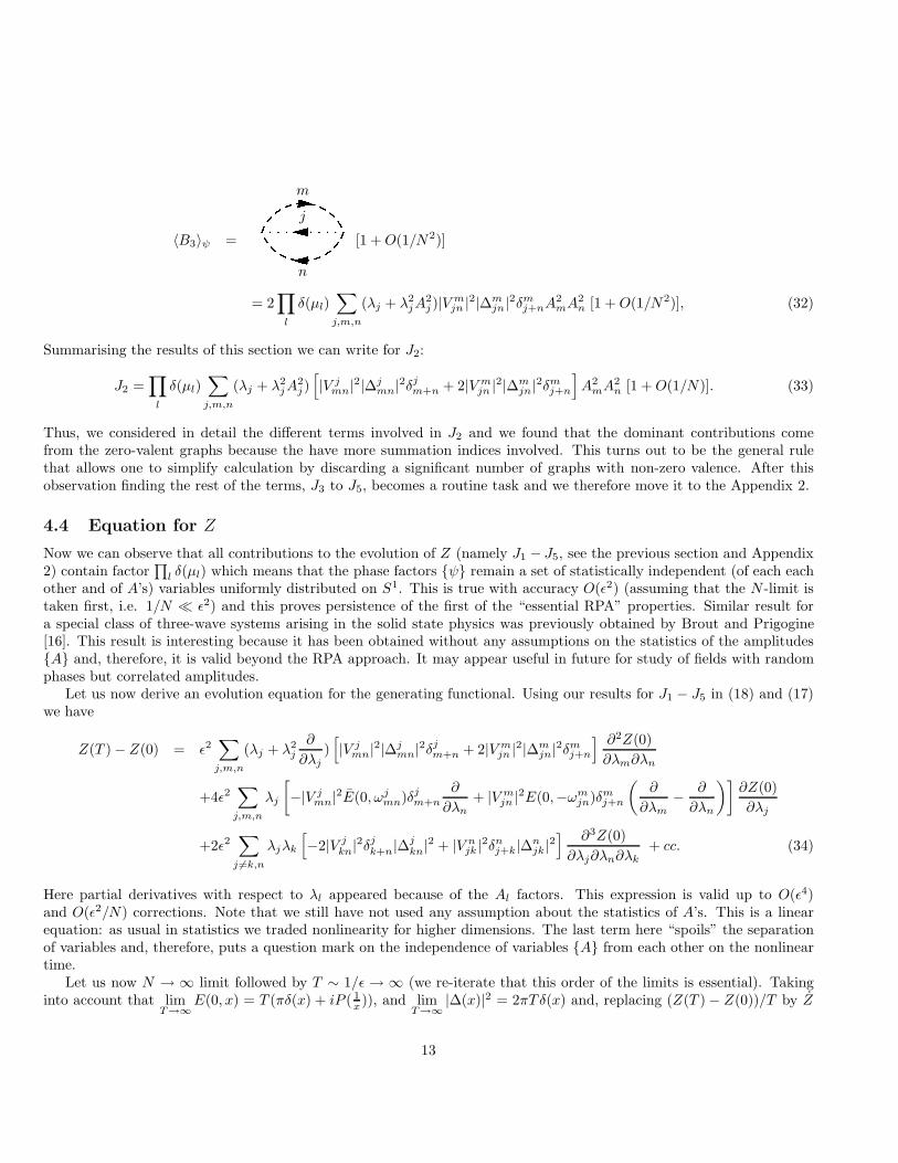
Similarly, the leading contribution to 〈B3〉ψ will be given by the zero-valent graph with the maximum possible numberof internal couplings (which is equal to 2 in this case). Because of the δ’s, there are no graphs with just one internalcoupling, but there are graphs with all the dashed lines coupled externally. Thus,

12

〈B3〉ψ =

m

j

n

[1 +O(1/N2)]

= 2∏

l

δ(µl)∑

j,m,n

(λj + λ2jA

2j )|V mjn |2|∆m

jn|2δmj+nA2mA

2n [1 +O(1/N2)], (32)

Summarising the results of this section we can write for J2:

J2 =∏

l

δ(µl)∑

j,m,n

(λj + λ2jA

2j)[

|V jmn|2|∆jmn|2δjm+n + 2|V mjn |2|∆m

jn|2δmj+n]

A2mA

2n [1 +O(1/N)]. (33)

Thus, we considered in detail the different terms involved in J2 and we found that the dominant contributions comefrom the zero-valent graphs because the have more summation indices involved. This turns out to be the general rulethat allows one to simplify calculation by discarding a significant number of graphs with non-zero valence. After thisobservation finding the rest of the terms, J3 to J5, becomes a routine task and we therefore move it to the Appendix 2.

4.4 Equation for Z

Now we can observe that all contributions to the evolution of Z (namely J1 − J5, see the previous section and Appendix2) contain factor

∏

l δ(µl) which means that the phase factors ψ remain a set of statistically independent (of each eachother and of A’s) variables uniformly distributed on S1. This is true with accuracy O(ǫ2) (assuming that the N -limit istaken first, i.e. 1/N ≪ ǫ2) and this proves persistence of the first of the “essential RPA” properties. Similar result fora special class of three-wave systems arising in the solid state physics was previously obtained by Brout and Prigogine[16]. This result is interesting because it has been obtained without any assumptions on the statistics of the amplitudesA and, therefore, it is valid beyond the RPA approach. It may appear useful in future for study of fields with randomphases but correlated amplitudes.

Let us now derive an evolution equation for the generating functional. Using our results for J1 − J5 in (18) and (17)we have

Z(T ) − Z(0) = ǫ2∑

j,m,n

(λj + λ2j

∂

∂λj)[

|V jmn|2|∆jmn|2δjm+n + 2|Vmjn |2|∆m

jn|2δmj+n] ∂2Z(0)

∂λm∂λn

+4ǫ2∑

j,m,n

λj

[

−|V jmn|2E(0, ωjmn)δjm+n

∂

∂λn+ |V mjn |2E(0,−ωmjn)δmj+n

(∂

∂λm− ∂

∂λn

)]∂Z(0)

∂λj

+2ǫ2∑

j 6=k,n

λjλk

[

−2|V jkn|2δjk+n|∆

jkn|2 + |V njk |2δnj+k|∆n

jk|2] ∂3Z(0)

∂λj∂λn∂λk+ cc. (34)

Here partial derivatives with respect to λl appeared because of the Al factors. This expression is valid up to O(ǫ4)and O(ǫ2/N) corrections. Note that we still have not used any assumption about the statistics of A’s. This is a linearequation: as usual in statistics we traded nonlinearity for higher dimensions. The last term here “spoils” the separationof variables and, therefore, puts a question mark on the independence of variables A from each other on the nonlineartime.

Let us now N → ∞ limit followed by T ∼ 1/ǫ → ∞ (we re-iterate that this order of the limits is essential). Takinginto account that lim

T→∞E(0, x) = T (πδ(x) + iP ( 1

x)), and limT→∞

|∆(x)|2 = 2πTδ(x) and, replacing (Z(T ) − Z(0))/T by Z

13

we have

Z = 4πǫ2∫(λj + λ2

j

δ

δλj)[

|V jmn|2δ(ωjmn)δjm+n + 2|Vmjn |2δ(ωmjn)δmj+n

] δ2Z

δλmδλn

+2λj

[

−|V jmn|2δ(ωjmn)δjm+n

δ

δλn+ |V mjn |2δ(ωmjn)δmj+n

(δ

δλm− δ

δλn

)]δZ

δλj

+2λjλm

[

−2|V jmn|2δjm+nδ(ωjmn) + |V njm|2δnj+mδ(ωnjm)

] δ3Z

δλjδλnδλm

dkjdkmdkn. (35)

Here variational derivatives appeared instead of partial derivatives because of the N → ∞ limit.

4.5 Equation for the PDF

Taking the inverse Laplace transform of (35) we have the following equation for the PDF,

P = −∫δFjδsj

dkj , (36)

where Fj is a flux of probability in the space of the amplitude sj,

Fj = 4πǫ2∫(|V jmn|2δ(ωjmn)δjm+n + 2|V njm|2δ(ωnjm)δnj+m)

[

snsmP − δ

δsj(sjsnsmP)

]

−2P[

|V jmn|2δ(ωjmn)δjm+nsjsm + |V njm|2δ(ωnjm)δnj+m(sjsm − sjsn)]

−2(|V njm|2δ(ωnjm)δnj+m − 2|V jmn|2δ(ωjmn)δjm+n)δ

δsm(sjsnsmP)

dkmdkn. (37)

This expression can be simplified to

− Fj4πǫ2sj

=

∫(|V jmn|2δ(ωjmn)δjm+n + 2|V njm|2δ(ωnjm)δnj+m)snsm

δPδsj

+2P(|V njm|2δ(ωnjm)δnj+m − |V jmn|2δ(ωjmn)δjm+n)sm

+2(|V njm|2δ(ωnjm)δnj+m − 2|V jmn|2δ(ωjmn)δjm+n)snsmδPδsm

dkmdkn. (38)

This equation is identical to the one originally obtained by Peierls [15] and later rediscovered by Brout and Prigogine [16]in the context of the physics of anharmonic crystals. Zaslavski and Sagdeev [17] were the first to study this equation inthe WT context. However, the analysis of [15, 16, 17] was restricted to the interaction Hamiltonians of the “potentialenergy” type, i.e. the ones that involve only the coordinates but not the momenta. This restriction leaves aside a greatmany important WT systems, e.g. the capillary, Rossby, internal and MHD waves. Our result above indicates that thePeierls equation is also valid in the most general case of 3-wave systems.

Here we should again emphasise importance of the taken order of limits, N → ∞ first and ǫ → 0 second. Physicallythis means that the frequency resonance is broad enough to cover great many modes. Some authors, e.g. [15, 16, 17], leavethe sum notation in the PDF equation even after the ǫ→ 0 limit taken giving δ(ωnjm). One has to be careful interpretingsuch formulae because formally the RHS is nill in most of the cases because there may be no exact resonances betweenthe discrete k modes (as it is the case, e.g. for the capillary waves). In real finite-size physical systems, this conditionmeans that the wave amplitudes, although small, should not be too small so that the frequency broadening is sufficient toallow the resonant interactions. Our functional integral notation is meant to indicate that the N → ∞ limit has alreadybeen taken.

14

5 Approximate independence of the amplitudes.

Variables sj do not separate in the above equation for the PDF. Indeed, substituting

P(N,a) = P(a)j1P

(a)j2

. . . P(a)jN

(39)

into the discrete version of (38) we see that it turns into zero on the thermodynamic solution with P(a)j = ωj exp(−ωjsj).

However, it is not zero for the one-mode PDF P(a)j corresponding to the cascade-type Kolmogorov-Zakharov (KZ) spec-

trum nkzj , i.e. P(a)j = (1/nkzj ) exp(−sj/nkzj ) (see next section), nor it is likely to be zero for any other PDF of form (39).

This means that, even initially independent, the amplitudes will correlate with each other at the nonlinear time. Doesthis mean that the existing WT theory, and in particular the kinetic equation, is invalid?

To answer to this question let us differentiate the discrete version of the equation (35) with respect to λ’s to getequations for the amplitude moments. We can easily see that

∂t(〈A2

j1A2j2〉 − 〈A2

j1〉〈A2j2 〉)

= O(ǫ4) (j1, j2 ∈ BN) (40)

if 〈A2j1A2j2A2j3〉 = 〈A2

j1〉〈A2

j2〉〈A2

j3〉 (with the same accuracy) at t = 0. Similarly, in terms of PDF’s

∂t

(

P(2,a)j1,j2

(sj1 , sj2) − P(a)j1

(sj1)P(a)j2

(sj2 ))

= O(ǫ4) (j1, j2 ∈ BN) (41)

if P(4,a)j1,j2,j3,j4

(sj1 , sj2 , sj3 , sj4) = P(a)j1

(sj1)P(a)j2

(sj2)P(a)j3

(sj3)P(a)j4

(sj4 ) at t = 0. Here P(4,a)j1,j2,j3,j4

(sj1 , sj2 , sj3 , sj4), P(2,a)j1,j2

(sj1 , sj2)

and P(a)j (sj) are the four-mode, two-mode and one-mode PDF’s obtained from P by integrating out all but 3,2 or 1 ar-

guments respectively. One can see that, with a ǫ2 accuracy, the Fourier modes will remain independent of each other inany pair over the nonlinear time if they were independent in every triplet at t = 0.

Similarly, one can show that the modes will remain independent over the nonlinear time in any subset of M < Nmodes with accuracy M/N (and ǫ2) if they were initially independent in every subset of size M + 1. Namely

P(M,a)j1,j2,...,jM

(sj1 , sj2 , sjM ) − P(a)j1

(sj1)P(a)j2

(sj2 ) . . . P(a)jM

(sjM ) = O(M/N) +O(ǫ2)

(j1, j2, . . . , jM ∈ BN) (42)

if P(M+1,a)j1,j2,...,jM+1

= P(a)j1P

(a)j2

. . . P(a)jM+1

at t = 0.

Mismatch O(M/N) arises from some terms in the ZS equation with coinciding indices j. For M = 2 there is onlyone such term in the N -sum and, therefore, the corresponding error is O(1/N) which is much less than O(ǫ2) (due to theorder of the limits in N and ǫ). However, the number of such terms grows as M and the error accumulates to O(M/N)which can greatly exceed O(ǫ2) for sufficiently large M .

We see that the accuracy with which the modes remain independent in a subset is worse for larger subsets and thatthe independence property is completely lost for subsets approaching in size the entire set, M ∼ N . One should notworry too much about this loss because N is the biggest parameter in the problem (size of the box) and the modes willbe independent in all M -subsets no matter how large. Thus, the statistical objects involving any finite number of modesare factorisable as products of the one-mode objects and, therefore, the WT theory reduces to considering the one-modeobjects. This results explains why we re-defined RPA in its relaxed “essential RPA” form. Indeed, in this form RPAis sufficient for the WT closure and, on the other hand, it remains valid over the nonlinear time. In particular, onlyproperty (40) is needed, as far as the amplitude statistics is concerned, for deriving the 3-wave kinetic equation, and thisfact validates this equation and all of its solutions, including the KZ spectrum which plays an important role in WT.

The situation were modes can be considered as independent when taken in relatively small sets but should be treatedas dependent in the context of much larger sets is not so unusual in physics. Consider for example a distribution ofelectrons and ions in plasma. The full N -particle distribution function in this case satisfies the Liouville equation which

15

is, in general, not a separable equation. In other words, the N -particle distribution function cannot be written as aproduct of N one-particle distribution functions. However, an M -particle distribution can indeed be represented as aproduct of M one-particle distributions if M ≪ ND where ND is the number of particles in the Debye sphere. We seean interesting transition from a an individual to collective behaviour when the number of particles approaches ND. Inthe special case of the one-particle function we have here the famous mean-field Vlasov equation which is valid up toO(1/ND) corrections (representing particle collisions).

6 One-mode statistics

We have established above that the one-point statistics is at the heart of the WT theory. All one-point statistical objectscan be derived from the one-point amplitude generating function,

Za(λj) =⟨

eλjA2j

⟩

which can be obtained from the N -point Z by taking all µ’s and all λ’s, except for λj , equal to zero. Substituting suchvalues to (35) we get the following equation for Za,

∂Za∂t

= λjηjZa + (λ2jηj − λjγj)

∂Za∂λj

, (43)

where,

ηj = 4πǫ2∫ (

|V jlm|2δjlmδ(ωjlm) + 2|V mjl |2δmjl δ(ωmjl )

)

nlnm dkldkm, (44)

γj = 8πǫ2∫ (

|V jlm|2δjlmδ(ωjlm)nm + |V mjl |2δmjl δ(ωmjl )(nl − nm)

)

dkldkm. (45)

Correspondingly, for the one mode PDF Pa(sj) we have

∂Pa∂t

+∂F

∂sj= 0, (46)

with F is a probability flux in the s-space,

F = −sj(γPa + ηjδPaδsj

). (47)

Equations (43) and (46) where previously obtained and studied in [20] in for the four-wave systems. The only differencefor the four-wave case was different expressions for η and γ. For the three-wave case, equation for the PDF was notconsidered before, but equations for its moments were derived and solved in [19]. In particular, equation for the firstmoment is nothing but the familiar kinetic equation n = −γn+ η which gives η = γn for any steady state. This, in turn

means that in the steady state with F = 0 we have P(a)j = (1/nj) exp(−sj/nj) where nj can be any steady state solution

of th kinetic equation including the KZ spectrum which plays the central role in WT [5, 1]. However, it was shown in[20] that there also exist solutions with F 6= 0 which describe WT intermittency.

7 Phase statistics.

Importantly, RPA formulation involves independent phase factors ψ = eφ and not phases φ themselves. Firstly, thephases would not be convenient because, as we will see later, the mean value of the phases is evolving and one couldnot say that they are “distributed uniformly from −π to π”. In fact, we will also see that the mean fluctuation of the

16

phase distribution is also growing and they quickly spread beyond their initial 2π-wide interval. But perhaps even moreimportant, φ’s build mutual correlations on the nonlinear time whereas ψ’s remain independent. This will be shown laterin this section, but we would like first to give a simple example illustrating how this property is possible due to the factthat correspondence between φ and ψ is not a bijection.

Let N be a random integer and let r1 and r2 be two independent (of N and of each other) random numbers withuniform distribution between −π and π. Let

φ1,2 = 2πN + r1,2.

Then〈φ1,2〉 = 2π〈N〉,

and〈φ1φ2〉 = 4π2〈N2〉.

Thus,〈φ1φ2〉 − 〈φ1〉〈φ2〉 = 4π2(〈N2〉 − 〈N〉2) > 0,

which means that variables φ1 and φ2 are correlated. On the other hand, if we introduce

ψ1,2 = eiφ1,2 ,

then〈ψ1,2〉 = 0,

and〈ψ1ψ2〉 = 0.

〈ψ1ψ2〉 − 〈ψ1〉〈ψ2〉 = 0,

which means that variables ψ1 and ψ2 are statistically independent. In this illustrative example it is clear that thedifference in statistical properties between φ and ψ arises from the fact that function ψ(φ) does not have inverse and,consequently, the information about N contained in φ is lost in ψ.

This illustration, although simple, captures the property that actually happens in reality as we will show below. Letus use the following expression for the phase

φj = ℑ ln aj .

Substituting (8) and Taylor-expanding of logarithm in ǫ one gets

φj = ℑ ln(a(0)j + ǫa

(1)j + ǫ2a

(2)j ) = φ(0) + ǫφ(1) + ǫ2φ(2) (48)

where

φ(0) = ℑ ln a(0)j , (49)

φ(1) = ℑa(1)j

a(0)j

, (50)

φ(2) = ℑ

−1

2

(

a(1)j

a(0)j

)2

+a(2)j

a(0)j

. (51)

Now let us perform averaging over the statistics of factors ψ(0). As usual, the surviving terms are those in which all ψ(0)’scancel out due to their pairwise matchings. This is possible only if the number of ψ(0)’s is equal to the number of ψ(0)’s

17

in the products defining these terms. Easy to see that the ǫ term involves three ψ(0)’s and therefore its average is zero.Therefore,

〈φj(T )〉 − 〈φ(0)j 〉 =

ǫ2

A2j

ℑ⟨

− 1

2A2j

(

a(1)j a

(0)j

)2

+ a(2)j a

(0)j

⟩

(52)

Let us consider

⟨

(a(1)j a

(0)j )2

⟩

=

⟨∑

m,n,κ,ν

(

V jmnaman∆jmnδ

jm+n + 2V mjnaman∆

mjnδ

mj+n

)(

V jκνaκaν∆jκνδ

jκ+ν + 2V κjνaκaν∆

mjnδ

mj+n

)

a2j

⟩

Here, there are two terms with equal number of ψ(0)’s and ψ(0)’s but all couplings of index j to any other index give zero

because V = 0 if one of its wavenumbers is zero. Thus,⟨

(a(1)j a

(0)j )2

⟩

= 0. The other term,⟨

a(2)j a

(0)j

⟩

ψhas already been

calculated before when evaluating J3. We have

⟨

a(2)j a

(0)j

⟩

ψ= 4

∑

m,n

[

−|V jmn|2E(0, ωjmn)δjm+nA

2n + |V mjn |2E(0,−ωmjn)δmj+n(A2

m −A2n)]

A2j

Let us take limits N → ∞ and T → ∞ and replace 〈φ(T )〉ψ − 〈φ(0)〉ψ/T by ˙〈φ〉ψ. We get

〈φj〉ψ = ωNL, (53)

where ωNL is the nonlinear frequency correction given by

ωNL = 4ǫ2∫[

|V jmn|2P(

1

ωjmn

)

δjm+n − |V mjn |2P(

1

ωmjn

)

δmj+n(A2m −A2

n)

]

A2j dkmdkn (54)

Here P(x) denotes the principal value of the integral. Averaging over the amplitudes, we have

˙〈φj〉 = 〈ωNL〉,

where 〈ωNL〉 is the amplitude-averaged nonlinear frequency correction

〈ωNL〉 = 4ǫ2∫[

|V jmn|2P(

1

ωjmn

)

δjm+n − |V mjn |2P(

1

ωmjn

)

δmj+n(nm − nn)

]

nj dkmdkn (55)

We can see that the mean value of the phase is steadily changing over the nonlinear time and, therefore, it would beincorrect to assume that the phase “remains uniformly distributed from −π to π” even though this could be true fort = 0. This is one of the reasons why we formulate RPA in terms of ψ and not φ. Indeed, ψ was shown above to stayuniformly distributed on the unit circle over the nonlinear time.

The other reason is that, strictly speaking, φ’s do not stay de-correlated where as ψ’s do (as shown before). Wealready saw in the beginning of this section that this situation is possible due to the fact that the map φ → ψ = eiφ

is not a bijection. Let us now study such a buildup in statistical dependence of the phases, let us consider correlatorFj,k ≡ 〈(φj − 〈φj〉)(φk − 〈φk〉)〉 = 〈φjφk〉 − 〈φj〉〈 φk〉. At time T we have

Fj,k(T ) = F (0)j,k + ǫF (1)

j,k + ǫ2F (2)j,k (56)

18

where

F (0)j,k = 〈φ(0)

j φ(0)k 〉 − 〈φ(0)

j 〉〈φ(0)k 〉,

F (1)j,k = 〈φ(1)

j φ(0)k 〉 + 〈φ(1)

k φ(0)j 〉,

F (2)j,k = 〈φ(1)

j φ(1)k 〉 + 〈φ(2)

j φ(0)k 〉 + 〈φ(2)

k φ(0)j 〉 − 〈φ(2)

j 〉〈φ(0)k 〉 − 〈φ(2)

k 〉〈φ(0)j 〉. (57)

Here, we have taken into account that, as we showed earlier, 〈φ(1)j 〉 = 0. Let us consider the ǫ-term F (1)

j,k , e.g.

〈φ(1)j φ

(0)k 〉 = ℑ〈(a(1)

j a(0)j )φ

(0)k 〉 = ℑ

∑

k,m,n

V jmn〈amanajφk〉∆jmnδ

jm+n + 2V mjn 〈amanajφk〉∆m

jnδmj+n (58)

In this expression, we have a factor φk which enters directly and not via the combination ψk = eiφk . Potentially, thiscould greatly complicate the situation because to objects like 〈ψkφk〉 knowledge of the statistics of ψ is not sufficient andone needs the full PDF of φk. Fortunately, however, this does not cause problems here because, no matter what index ismatched to k, matching of the two remaining indices results in V = 0. Therefore, the contribution of the ǫ-terms is nill.

Let us now consider the F (2)j,k starting with

〈φ(2)j φ

(0)k 〉ψ =

⟨

ℑ

−1

2

(

a(1)j

a(0)j

)2

+a(2)j

a(0)j

φ(0)k

⟩

= ℑ⟨[

− 1

2A4j

(a(1)j a

(0)j )2 +

1

A2j

a(2)j a

(0)j

]

φ(0)k

⟩

. (59)

We see that the square bracket on the RHS involves an even number (four or six) of ψ′s in each term. Thus, inorder for these terms to survive these ψ′s must cancel out which is possible when their indices match in a pairwiseway. But this means that index k (of φk) does not match to any of the indices of ψ′s and, therefore, the averaging ofφk can be taken separately because it is statistically independent of all other phase factors.5 Thus, we conclude that

〈φ(2)j φ

(0)k 〉ψ = 〈φ(2)

j 〉ψ〈φ(0)k 〉ψ and these terms drop out of F (2)

j,k . The remaining term in F (2)j,k is

〈φ(1)j φ

(1)k 〉ψ = −1

4

⟨(

a(1)j

a(0)j

−a(1)j

a(0)j

)(

a(1)j

a(0)j

−a(1)j

a(0)j

)⟩

= −1

4

⟨

a(1)j a

(1)k

a(0)j a

(0)k

−a(1)j a

(1)k

a(0)j a

(0)k

+ c.c

⟩

= 2|V jk(j−k)|2|∆j

k(j−k)|2A2

j−k + 2|V kj(k−j)|2|∆kj(k−j) |2A2

k−j + 2|V j+kjk |2|∆j+kjk |2A2

j+k

+δjkA2j

∑

l,m

[

|V jlm|2|∆jlm|2δjl+m + 2|V mjl |2|∆m

jl |2δml+j]

A2lA

2m (60)

We can now average over the amplitudes and take limits N → ∞ and ǫ→ 0 and write

Fj,k = 4πǫ2[

|V jk(j−k) |2δ(ωjk(j−k))nj−k + |V kj(k−j) |2δ(ωkj(k−j))nk−j + |V j+kjk |2δ(ωj+kjk )nj+k

]

+2πǫ2δjknj

∫ [

|V jlm|2δ(ωjlm)δjl+m + 2|V mjl |2δ(ωmjl )δml+j]

nlnm dkldkm. (61)

Presence of the 1-st term on the RHS indicates that the phases of the j-th and the k-th modes get correlated on thenonlinear time. This correlation is week in a sense that Fj,k has a sharp peak at j = k but the integrated contributionof all j 6= k is of the same order as the value at the contribution of the j = k peak and, therefore, could cause a problemshould one tried to build RPA based on the statistics of φ’s rather than ψ’s (which remain de-correlated).

5There is of course also a possibility that k couples simultaneously to both indices in a pair, but this contribution contains ∼ 1/N less termsand, therefore, should be ignored.

19

Let us consider a special case of (61) for j = k which is interesting because it allows one to calculate the dispersion inphases,

σk = 〈φ2k〉 − 〈φk〉2

We haveσk = ηk/nk, (62)

where ηk is defined in (44) and nk = 〈|ak|2〉. One can see that the RHS here is always positive and, therefore, the phasefluctuations experience an unlimited growth. On stationary spectra, this growth is ∼

√t which corresponds to σ ∼ t.

Recall that the mean value of the phase is also changing in time with the rate ωNL and on stationary spectra this changeis linear in time.

8 Discussion

In the present paper, we considered evolution of the full N-mode objects such as the generating functional and theprobability density function for all the wave amplitudes and their phase factors. We proved that the phase factors, beingstatistically independent and uniform on S1 initially, remain so over the nonlinear evolution time in the leading order insmall nonlinearity. If in addition the initial amplitudes are independent too, then they remain so over the nonlinear timein a weak sense. Namely, all joint PDF’s for the number of modes M ≪ N split into products of the one-mode densitieswith O(M/N) and O(ǫ2) accuracy. Thus, the full N -mode PDF does not factorise as a product of N one-mode densitiesand the Fourier modes in the set considered as a whole are not independent. However, the wave turbulence closure onlydeals with the joint objects of the finite size M of variables while taking N → ∞ limit. These objects do factorise intoproducts and, for the WT purposes, the Fourier modes can be interpreted as statistically independent. In particular, thederivation of the kinetic equation for the energy spectrum deals only with the 1-mode and the 2-mode distributions andis, therefore, justified by the results of the present paper. Generally speaking, our results reduce the leading-order WTproblem to the study of the one-mode amplitude PDF’s and they validate the generalised RPA technique introduced in[19, 20]. Such a study of the one-mode PDF and the high-order momenta of the wave amplitudes was done in [19, 20].It was shown, in particular, that anomalous probabilities of large wave amplitudes can appear in the form of a finite-fluxsolution in the amplitude space caused by a wave-breaking amplitude cutoff. The reader is referred to these papers forthe discussion of the WT intermittency.

Although our results indicate that correlations between 2 or more (but ≪ N) modes do not appear in the leading(i.e. ǫ2) order for the three-wave systems, they definitely appear as corrections in the next (i.e. ǫ4) order. Our paperis concerned with the main order statistics only in which the main evolution happens in the 1-mode objects, e.g. the1-mode amplitude distributions. For study of the multi-mode correlations developing in WT in the next order in ǫ thereader is referred to papers [21, 22].

We have also considered correlators of the phase and we showed the relation between the statistical properties of thephase φ and the phase factors ψ = eiφ. We showed that the mean of φ and its fluctuations about the mean grow in timeand, therefore, there exist no 2π-wide interval in which the phase would remain uniformly distributed. Moreover, phasesφ become correlated at different wavenumbers that lie on the resonant manifold. These properties make the phase φ aninappropriate variable for formulating the RPA method of WT description. On the other hand, our work shows that thephase factors ψ = eiφ do remain statistically independent and uniform on S1 which makes them the right choice for theRPA formulation.

The present paper deals with the three-wave systems only. The four-wave resonant interactions are slightly morecomplicated in that the nonlinear frequency shift occurs at a lower order in nonlinearity parameter than the nonlinearevolution of the wave amplitudes. To build a consistent description of the amplitude moments one has to perform arenormalisation of the perturbation series taking into account the nonlinear frequency shift. This derivation will bepublished separately, whereas here we just announce its main result, the 4-wave generalisation of the Peierls equation for

20

the PDF. It has the same continuity equation form (36) but now the probability flux is

Fj = 4πǫ4∑

123

W j123 δ(ω

ji23)δ

j123s1s2s3sj(

δ

δsj+

δ

δs1− δ

δs2− δ

δs3)P, (63)

where W j123 is the 4-wave ineraction coefficient and ωlαµν = ωlαµν + Ωl + Ωα − Ωµ − Ων with Ωl = 2ǫ

∑

µWlµlµ nµ being

the nonlinear frequency shift. As wee see this equation is even more compact than its 3-wave analog. In additionto the derivation of this equation, we will also analyse its properties and consequences for the mode correlations andintermittency in 4-wave turbulent systems.

9 Appendix 1

Let us obtain Z(T ) in terms of the series in small nonlinearity up to the second order in ǫ. As an intermediate step, wefirst consider separately the amplitude and the phase ingredients of Z and substitute the ǫ-expansion of a from (8) intotheir expressions,

eλj |aj |2

= eλj |a(0)

j+ǫa

(1)

j+ǫ2a

(2)

j|2 = e

λj |a(0)

j|2+ǫλj(a

(1)

ja(0)

j+a

(1)

ja(0)

j)+ǫ2λj

[|a

(1)

j|2+(a

(2)

ja(0)

j+a

(2)

ja(0)

j)]

= eλj |a(0)j

|2

1 + ǫλj(a(1)j a

(0)j + a

(1)j a

(0)j ) + ǫ2λj

[

|a(1)j |2 + (a

(2)j a

(0)j + a

(2)j a

(0)j )]

+ǫ2λ2

j

2(a

(1)j a

(0)j + a

(1)j a

(0)j )2

= eλjA(0)2

j (1 + ǫα1j + ǫ2α2j), (64)

and

ψµj

j =

(

a(0)j + ǫa

(1)j + ǫ2a

(2)j

a(0)j + ǫa

(1)j + ǫ2a

(2)j

)µj

2

= ψ(0)µj

j

1 + ǫa(1)j

a(0)

j

+ ǫ2a(2)j

a(0)

j

1 + ǫa(1)

j

a(0)j

+ ǫ2a(2)

j

a(0)j

µj

2

= ψ(0)µj

j

1 + ǫµj2

a(1)j

a(0)j

+ ǫ2µj2

a(2)j

a(0)j

+ǫ2

2

µj2

(µj2

− 1)(

a(1)j

a(0)j

)2

1 − ǫµj2

a(1)j

a(0)j

− ǫ2µj2

a(2)j

a(0)j

+ǫ2

2

µj2

(µj2

+ 1)(

a(1)j

a(0)j

)2

= ψ(0)µj

j

1 + ǫ

µj2

(

a(1)j

a(0)j

−a(1)j

a(0)j

)

+ ǫ2

µj2

(

a(2)j

a(0)j

−a(2)j

a(0)j

)

+µj4

(µj2

− 1)(

a(1)j

a(0)j

)2

+(µj

2+ 1)(

a(1)j

a(0)j

)2

−µ2j |a

(1)j |2

4A(0)2j

= ψ(0)µj

j (1 + ǫβ1j + ǫ2β2j), (65)

where α1j , α2j , β1j and β2j denote the linear and quadratic contributions into the amplitude and phase parts of Zrespectively,

α1j = λj(a(1)j a

(0)j + a

(1)j a

(0)j ), (66)

α2j = (λj + λ2jA

(0)2j |a(1)

j |2 + λj(a(2)j a

(0)j + a

(2)j a

(0)j ) +

λ2j

2(a

(1)j a

(0)j )2 + (a

(1)j a

(0)j )2, (67)

β1j =µj

2A(0)2j

(a(1)j a

(0)j − a

(1)j a

(0)j ), (68)

β2j =µj

2A(0)2j

(a(2)j a

(0)j − a

(2)j a

(0)j ) +

µj4

(µj2

− 1)(

a(1)j

a(0)j

)2

+(µj

2+ 1)(

a(1)j

a(0)j

)2

−µ2j |a

(1)j |2

4A(0)2j

. (69)

21

Substituting expansions (64) and (65) into the expression for Z, we have

Z(T ) =1

(2π)N

⟨∏

l

eλl|al|2

(alal

)µl2

⟩

=1

(2π)N

⟨∏

l

eλlA(0)2

l [1 + ǫα1l + ǫ2α2l]ψ(0)µl

l [1 + ǫβ1l + ǫ2β2l]

⟩

=1

(2π)N

⟨∏

l

eλlA(0)2

l ψ(0)µl

l

1 + ǫ∑

j

(α1j + β1j) + ǫ2∑

j

(α2j + β2j) + ǫ2∑

j<k

(α1jα1k + β1jβ1k) +∑

j,k

α1jβ1k

⟩

=1

(2π)N

⟨∏

l

eλlA(0)2

l ψ(0)µl

l

[1 + ǫ

∑

j

(α1j + β1j)

︸ ︷︷ ︸

I1

+ǫ2∑

j

(α2j + β2j + α1jβ1j)

︸ ︷︷ ︸

I2

+ǫ21

2

∑

j 6=k

(α1jα1k + β1jβ1k + 2α1jβ1k)

︸ ︷︷ ︸

I3

]

⟩

,

For parts I1, I2 and I3 in the above expression we have,

I1 =∑

j

(λj +µj

2A2j

)a(1)j a

(0)j + (λj −

µj2A2

j

)a(1)j a

(0)j ,

I2 =∑

j

(λj + λ2jA

2j −

µ2j

2A2j

)|a(1)j |2 + (λj +

µj2A2

j

)a(2)j a

(0)j + (λj −

µj2A2

j

)a(2)j a

(0)j

+

[

λ2j

2+

µj4A4

j

(µj2

− 1)

+λjµj2A2

j

]

(a(1)j a

(0)j )2 +

[

λ2j

2+

µj4A4

j

(µj2

+ 1)

− λjµj2A2

j

]

(a(1)j a

(0)j )2,

I3 =1

2

∑

j 6=k

[λjλk(a

(1)j a

(0)j + a

(1)j a

(0)j )(a

(1)k a

(0)k + a

(1)k a

(0)k ) +

λjµkA2k

(a(1)j a

(0)j + a

(1)j a

(0)j )(a

(1)k a

(0)k − a

(1)k a

(0)k )

+µjµk

4A2jA

2k

(a(1)j a

(0)j − a

(1)j a

(0)j )(a

(1)k a

(0)k − a

(1)k a

(0)k )],

Exploiting the property Zλ,−µ = Zλ, µ we can write

Zλ, µ = Xλ, µ + Xλ,−µ. (70)

At t = T we have for Xλ, µ

X(T ) = X(0) + (2π)2N

⟨∏

‖l‖<N

eλl|a(0)

l|2 [ǫJ1 + ǫ2(J2 + J3 + J4 + J5)]

⟩

A

, (71)

where

J1 =

⟨∏

l

ψ(0)µl

l

∑

j

(λj +µj

2|a(0)j |2

)a(1)j a

(0)j

⟩

ψ

, (72)

J2 =1

2

⟨∏

l

ψ(0)µl

l

∑

j

(λj + λ2j |a

(0)j |2 −

µ2j

2|a(0)j |2

)|a(1)j |2

⟩

ψ

, (73)

22

J3 =

⟨∏

l

ψ(0)µl

l

∑

j

(λj +µj

2|a(0)j |2

)a(2)j a

(0)j

⟩

ψ

, (74)

J4 =

⟨∏

l

ψ(0)µl

l

∑

j

[

λ2j

2+

µj

4|a(0)j |4

(µj2

− 1)

+λjµj

2|a(0)j |2

]

(a(1)j a

(0)j )2

⟩

ψ

, (75)

J5 =1

2

⟨∏

l

ψ(0)µl

l

∑

j 6=k

λjλk(a(1)j a

(0)j + a

(1)j a

(0)j )a

(1)k a

(0)k + (λj +

µj

4|a(0)j |2

)µk

|a(0)k |2

(a(1)k a

(0)k − a

(1)k a

(0)k )a

(1)j a

(0)j

⟩

ψ

, (76)

where 〈·〉A and 〈·〉ψ denote the averaging over the initial amplitudes and initial phases respectively. We remind that suchindividual averages are possible because the amplitudes and the phases are statistically independent from each other att = 0.

10 Appendix 2

10.1 Calculation of J3

J3 =

⟨∏

l

ψ(0)µl

l

∑

j

(λj +µj

2A2j

)a(2)j a

(0)j

⟩

ψ

= 〈∏

l

ψ(0)µl

l

∑

j

(λj +µj

2A2j

)

∑

j,m,n,κ,ν

[

2V jmn(−VmκνanaκaνE[ωjnκν , ω

jmn]δ

mκ+ν − 2V κmνanaκaνE[ωjνnκ, ω

jmn]δ

κm+ν

)δjm+n

+2Vmjn(−Vmκν anaκaνE[ωjnκν ,−ωmjn]δmκ+ν − 2V κmν anaκaνE[−ωκnνj ,−ωmjn]δκm+ν

)δmj+n

+2Vmjn(V nκνamaκaνδ

nκ+νE[−ωmjνκ,−ωmjn] + 2V κnνamaκaνE[ωκjνm,−ωmjn]δκn+ν

)δmj+n

]aj〉ψ . (77)

The terms to be averaged here can be drawn as

m

j

n

κ

ν

+

m

j

n

κ

ν

+

m

j

n

κ

ν

+

m

j

n

κ

ν

+

n

j

m

κ

ν

+

n

j

m

κ

ν

(78)

23

Let us now average over the random phases. Again, the leading order terms will be given by the diagrams with thelargest number of internal couplings. They will arise from the V V terms (the 2nd, 3rd and the 6th graphs) because theyallow 2 internal couplings in each of them. There are also possibilities to have one internal and two external couplings ofthe dashed lines, - such terms will give a O(1/N) correction to the leading order. Therefore,

J3 =

m

n

j

+ 2

m

n

j

+

m

n

j

[1 +O(1/N)]

= 4∏

l

δ(µl)∑

j,m,n

λj

[

−|V jmn|2E(0, ωjmn)δjm+nA

2n + |V mjn |2E(0,−ωmjn)δmj+n(A2

m −A2n)]

A2j

×[1 +O(1/N)] (79)

10.2 Calculation of J4

J4 =

⟨∏

l

ψ(0)µl

l

∑

j

[

λ2j

2+

µj4A4

j

(µj2

− 1)

+λjµj2A2

j

]

(a(1)j a

(0)j )2

⟩

ψ

= 〈∏

l

ψµl

l

∑

j,m,n,κ,ν

[

λ2j

2+

µj4A4

j

(µj2

− 1)

+λjµj2A2

j

]

(

V jmnaman∆jmnδ

jm+n + 2Vmjnaman∆

mjnδ

mj+n

)(

V jκνaκaν∆jκνδ

jκ+ν + 2V κjνaκaν∆

mjnδ

mj+n

)

a2j〉ψ. (80)

Graphically, the 4 terms to be averaged in this expression are

m

n

κ

ν

j

+

m

n

κ

ν

j

+

m

n

κ

ν

j

+

m

n

κ

ν

j

Note that there is no dotted lines in these graphs because for each summation index there is a corresponding waveamplitude present. As a consequence, the rule for the number of surviving summations is somewhat different from whatwe had so far. Namely, the number of the summation indices after the phase averaging is one less than the number of thepurely internal couplings. Easy to see that the phase averaging of the above terms always leads to an external coupling

24

of the dashed lines j which removes the j summation. Moreover, no more than one purely internal coupling of the dashedlines is possible in any of these graphs. 6 Thus, J4 contains no summation at all and is only a O(1/N2) correction to themain terms in J2 and J3.

10.3 Calculation of J5

Expression for J5 seemingly involves a great number terms. However, this number can be dramatically reduced by thefollowing speculation. Just as in J4 there is no dotted lines in the graphs involved in J5 because for each summation indexthere is a corresponding wave amplitude present. Thus, we have the same rule for the number of summations survivingthe phase averaging (i.e. one less than the number of internal couplings). In order to be of the same order as the leadingterms in J2 and J3, we must have 3 purely internal couplings and, therefore, no external couplings. This is only possiblewhen the number of dotted lines directed to the vertices is equal to the number of them pointing away which is true forthe V V terms but not true for the V V and V V terms. Thus we will only consider the V V terms. Further, the fact thatthere is no external couplings means that such terms are only non-zero when all µ’s are zero. Thus, there will be nocontribution from the second part of J5 which has a µk pre-factor.

J5 =1

2

⟨∏

l

ψ(0)µl

l

∑

j 6=k

λjλk(a(1)j a

(0)j + a

(1)j a

(0)j )a

(1)k a

(0)k

⟩

ψ

[1 +O(1/N)], (81)

where the V V terms to be averaged here are

C1 =

m

n

κ

ν

j

k

= −∏

l

ψ(0)µl

l

∑

j 6=k,m,n,µ,ν

λjλkVjmnδ

jm+namanaj V

κkνδ

κk+νaκaν ak∆

jmn∆

κkν ,

C2 =

m

n

κ

ν

j

k

= −∏

l

ψ(0)µl

l

∑

j 6=k,m,n,µ,ν

λjλkVmjnδ

mj+namanajV

kκνδ

kκ+νaκaν ak∆

mjn∆k

κν ,

C3 =

m

n

κ

ν

j

k6The only possibility of the double internal coupling would be in the last graph via joining m with ν and κ with n, but this would mean

j = 0 because of the δ-symbols and, therefore, this term is nill.

25

= 2∏

l

ψ(0)µl

l

∑

j 6=k,m,n,µ,ν

λjλkVmjnδ

mj+namanaj V

κkνδ

κk+νaκaν ak∆

mjn∆κ

kν ,

C4 =

m

n

κ

ν

j

k

=1

2

∏

l

ψ(0)µl

l

∑

j 6=k,m,n,µ,ν

λjλkVjmnδ

jm+namanajV

kκνδ

kκ+νaκaν ak∆

jmn∆

kκν .

By coupling the dashed lines we have in the leading order

〈C1〉ψ = 2

n

k

j= −2

∏

l

δ(µl)∑

j 6=k,n

λjλk|V jkn|2δjk+nA

2jA

2nA

2k|∆j

kn|2,

〈C2〉ψ = 2

k

j

n

= −2∏

l

δ(µl)∑

j 6=k,n

λjλk|V kjn|2δkj+nA2jA

2nA

2k|∆k

jn|2 = 〈C1〉ψ,

〈C3〉ψ =

j

k

m

= 2∏

l

δ(µl)∑

j 6=k,m

λjλk|V mjk |2δmj+kA2jA

2mA

2k|∆m

jk|2.

Term C4 does not survive the averaging because j 6= k and a triple internal coupling is not possible. Summarising,

J5 = 2∏

l

δ(µl)∑

j 6=k,n

λjλk

[

−2|V jkn|2δjk+n|∆

jkn|2 + |V njk|2δnj+k|∆n

jk|2]

A2jA

2nA

2k [1 +O(1/N)]. (82)

References

[1] V.E. Zakharov, V.S. L’vov and G.Falkovich, ”Kolmogorov Spectra of Turbulence”, Springer-Verlag, 1992.

[2] D.J. Benney and P.Saffman, Proc Royal. Soc, A(1966), 289, 301-320; B. J . Benney and A.C. Newell, Studies inAppl. Math. 48 (1) 29 (1969).

26

[3] A.A. Galeev and R.Z. Sagdeev, in “Reviews of Plasma Physics” Vol. 6 (Ed. M A Leontovich) (New York: ConsultantsBureau, 1973)

[4] A.C. Newell: Rev. Geophys. 6, 1 (1968)

[5] V.E.Zakharov and Filonenko, J. Appl. Mech. Tech. Phys. 4 506-515 (1967).

[6] K. Hasselmann, J. Fluid Mech 12 481 (1962). “ Freely decaying weak turbulence for sea surface gravity waves “

[7] S. Dyachenko, A.C. Newell, A. Pushkarev, V.E. Zakharov: Physica D 57, 96 (1992)

[8] H.W. Wyld, Ann. Phys. 14 (1961) 143.

[9] V.S. Lvov, Y.V. Lvov, A.C. Newell and V.E. Zakharov, “Statistical description of acoustic turbulence” Phys. Rev.E 56 (1997) 390.

[10] V.E. Zakharov, V.S. Lvov, Izv. Vuzov Radiophys. vol. XVIII (1975) 1470

[11] R.C. Davidson “Methods in Nonlinear Plasma Theory”, New York: Academic Press 1972.

[12] A.N. Pushkarev, V.E. Zakharov, “ Turbulence of capillary waves” PRL 76, 3320-3, (1996). Physica D, 135, 98,(2000).

[13] A.M.Balk and S.V. Nazarenko “On the Physical Realizability of Anisotropic Kolmogorov Spectra of Weak Turbu-lence” Sov.Phys.-JETP 70 (1990) 1031.

[14] Yu. V. Lvov and E.G. Tabak, PRL 87, 168501, (2001)

[15] R. Peierls, Annalen Physik 3 (1029) 1055.

[16] R. Brout and I. Prigogine, Physica 22 (1956) 621-636.

[17] G.M. Zaslavskii and R.Z. Sagdeev, Sov.Phys. JETP 25 (1967) 718.

[18] V.E. Zakharov, P. Guyenne, A.N. Pushkarev, F. Dias, Physica D 152-153 573-619 (2001)

[19] Yu. Lvov and Sergey Nazarenko, Spectral fluctuations, long correlations and intermittency in Wave Turbulence, toappear in PRE (2004). Also at http://arxiv.org/abs/math-ph/0305028.

[20] Y. Choi, Yu. Lvov and S.V. Nazarenko, Anomalous probability of high amplitudes in wave turbulence, submittedto PRL. Also at http://arxiv.org/abs/math-ph/0404022

[21] L. Biven, S.V. Nazarenko and A.C. Newell, ”Breakdown of wave turbulence and the onset of intermittency”, PhysLett A, 280, 28-32, (2001); A.C. Newell, S.V. Nazarenko and L. Biven, Physica D, 152-153, 520-550, (2001).

[22] P.A.E.M. Janssen, “Nonlinear four-wave interactions and freak waves”

27