Global carbon budget 2014
39
Earth Syst. Sci. Data, 7, 47–85, 2015 www.earth-syst-sci-data.net/7/47/2015/ doi:10.5194/essd-7-47-2015 © Author(s) 2015. CC Attribution 3.0 License. Global carbon budget 2014 C. Le Quéré 1 , R. Moriarty 1 , R. M. Andrew 2 , G. P. Peters 2 , P. Ciais 3 , P. Friedlingstein 4 , S. D. Jones 1 , S. Sitch 5 , P. Tans 6 , A. Arneth 7 , T. A. Boden 8 , L. Bopp 3 , Y. Bozec 9,10 , J. G. Canadell 11 , L. P. Chini 12 , F. Chevallier 3 , C. E. Cosca 13 , I. Harris 14 , M. Hoppema 15 , R. A. Houghton 16 , J. I. House 17 , A. K. Jain 18 , T. Johannessen 19,20 , E. Kato 21,22 , R. F. Keeling 23 , V. Kitidis 24 , K. Klein Goldewijk 25 , C. Koven 26 , C. S. Landa 19,20 , P. Landschützer 27 , A. Lenton 28 , I. D. Lima 29 , G. Marland 30 , J. T. Mathis 13 , N. Metzl 31 , Y. Nojiri 21 , A. Olsen 19,20 , T. Ono 32 , S. Peng 3 , W. Peters 33 , B. Pfeil 19,20 , B. Poulter 34 , M. R. Raupach 35,† , P. Regnier 36 , C. Rödenbeck 37 , S. Saito 38 , J. E. Salisbury 39 , U. Schuster 5 , J. Schwinger 19,20 , R. Séférian 40 , J. Segschneider 41 , T. Steinhoff 42 , B. D. Stocker 43,44 , A. J. Sutton 45,13 , T. Takahashi 46 , B. Tilbrook 47 , G. R. van der Werf 48 , N. Viovy 3 , Y.-P. Wang 49 , R. Wanninkhof 50 , A. Wiltshire 51 , and N. Zeng 52 1 Tyndall Centre for Climate Change Research, University of East Anglia, Norwich Research Park, Norwich NR4 7TJ, UK 2 Center for International Climate and Environmental Research – Oslo (CICERO), Oslo, Norway 3 Laboratoire des Sciences du Climat et de l’Environnement, Institut Pierre-Simon Laplace, CEA-CNRS-UVSQ, CE Orme des Merisiers, 91191 Gif sur Yvette Cedex, France 4 College of Engineering, Mathematics and Physical Sciences, University of Exeter, Exeter EX4 4QF, UK 5 College of Life and Environmental Sciences, University of Exeter, Exeter EX4 4QE, UK 6 National Oceanic & Atmospheric Administration, Earth System Research Laboratory (NOAA/ESRL), Boulder, CO 80305, USA 7 Karlsruhe Institute of Technology, Institute of Meteorology and Climate Research/Atmospheric Environmental Research, 82467 Garmisch-Partenkirchen, Germany 8 Carbon Dioxide Information Analysis Center (CDIAC), Oak Ridge National Laboratory, Oak Ridge, TN, USA 9 CNRS, UMR7144, Equipe Chimie Marine, Station Biologique de Roscoff, Place Georges Teissier, 29680 Roscoff, France 10 Sorbonne Universités (UPMC, Univ Paris 06), UMR7144, Adaptation et Diversité en Milieu Marin, Station Biologique de Roscoff, 29680 Roscoff, France 11 Global Carbon Project, CSIRO Oceans and Atmosphere Flagship, GPO Box 3023, Canberra, ACT 2601, Australia 12 Department of Geographical Sciences, University of Maryland, College Park, MD 20742, USA 13 National Oceanic & Atmospheric Administration/Pacific Marine Environmental Laboratory (NOAA/PMEL), 7600 Sand Point Way NE, Seattle, WA 98115, USA 14 Climatic Research Unit, University of East Anglia, Norwich Research Park, Norwich NR4 7TJ, UK 15 Alfred Wegener Institute Helmholtz Centre for Polar and Marine Research, Postfach 120161, 27515 Bremerhaven, Germany 16 Woods Hole Research Center (WHRC), Falmouth, MA 02540, USA 17 Cabot Institute, Department of Geography, University of Bristol, Bristol BS8 1TH, UK 18 Department of Atmospheric Sciences, University of Illinois, Urbana, IL 61821, USA 19 Geophysical Institute, University of Bergen, Allégaten 70, 5007 Bergen, Norway 20 Bjerknes Centre for Climate Research, Allégaten 55, 5007 Bergen, Norway 21 Center for Global Environmental Research, National Institute for Environmental Studies (NIES), 16-2 Onogawa, Tsukuba, Ibaraki 305-8506, Japan 22 Institute of Applied Energy (IAE), Minato-ku, Tokyo 105-0003, Japan 23 University of California, San Diego, Scripps Institution of Oceanography, La Jolla, CA 92093-0244, USA 24 Plymouth Marine Laboratory, Prospect Place, Plymouth PL1 3DH, UK Published by Copernicus Publications.
-
Upload
independent -
Category
Documents
-
view
2 -
download
0
Transcript of Global carbon budget 2014

Earth Syst. Sci. Data, 7, 47–85, 2015
www.earth-syst-sci-data.net/7/47/2015/
doi:10.5194/essd-7-47-2015
© Author(s) 2015. CC Attribution 3.0 License.
Global carbon budget 2014
C. Le Quéré1, R. Moriarty1, R. M. Andrew2, G. P. Peters2, P. Ciais3, P. Friedlingstein4, S. D. Jones1,
S. Sitch5, P. Tans6, A. Arneth7, T. A. Boden8, L. Bopp3, Y. Bozec9,10, J. G. Canadell11, L. P. Chini12,
F. Chevallier3, C. E. Cosca13, I. Harris14, M. Hoppema15, R. A. Houghton16, J. I. House17, A. K. Jain18,
T. Johannessen19,20, E. Kato21,22, R. F. Keeling23, V. Kitidis24, K. Klein Goldewijk25, C. Koven26,
C. S. Landa19,20, P. Landschützer27, A. Lenton28, I. D. Lima29, G. Marland30, J. T. Mathis13, N. Metzl31,
Y. Nojiri21, A. Olsen19,20, T. Ono32, S. Peng3, W. Peters33, B. Pfeil19,20, B. Poulter34, M. R. Raupach35,†,
P. Regnier36, C. Rödenbeck37, S. Saito38, J. E. Salisbury39, U. Schuster5, J. Schwinger19,20, R. Séférian40,
J. Segschneider41, T. Steinhoff42, B. D. Stocker43,44, A. J. Sutton45,13, T. Takahashi46, B. Tilbrook47,
G. R. van der Werf48, N. Viovy3, Y.-P. Wang49, R. Wanninkhof50, A. Wiltshire51, and N. Zeng52
1Tyndall Centre for Climate Change Research, University of East Anglia, Norwich Research Park,
Norwich NR4 7TJ, UK2Center for International Climate and Environmental Research – Oslo (CICERO), Oslo, Norway
3Laboratoire des Sciences du Climat et de l’Environnement, Institut Pierre-Simon Laplace,
CEA-CNRS-UVSQ, CE Orme des Merisiers, 91191 Gif sur Yvette Cedex, France4College of Engineering, Mathematics and Physical Sciences, University of Exeter, Exeter EX4 4QF, UK
5College of Life and Environmental Sciences, University of Exeter, Exeter EX4 4QE, UK6National Oceanic & Atmospheric Administration, Earth System Research Laboratory (NOAA/ESRL),
Boulder, CO 80305, USA7Karlsruhe Institute of Technology, Institute of Meteorology and Climate Research/Atmospheric
Environmental Research, 82467 Garmisch-Partenkirchen, Germany8Carbon Dioxide Information Analysis Center (CDIAC), Oak Ridge National Laboratory, Oak Ridge, TN, USA
9CNRS, UMR7144, Equipe Chimie Marine, Station Biologique de Roscoff, Place Georges Teissier,
29680 Roscoff, France10Sorbonne Universités (UPMC, Univ Paris 06), UMR7144, Adaptation et Diversité en Milieu Marin,
Station Biologique de Roscoff, 29680 Roscoff, France11Global Carbon Project, CSIRO Oceans and Atmosphere Flagship, GPO Box 3023, Canberra,
ACT 2601, Australia12Department of Geographical Sciences, University of Maryland, College Park, MD 20742, USA
13National Oceanic & Atmospheric Administration/Pacific Marine Environmental Laboratory (NOAA/PMEL),
7600 Sand Point Way NE, Seattle, WA 98115, USA14Climatic Research Unit, University of East Anglia, Norwich Research Park, Norwich NR4 7TJ, UK15Alfred Wegener Institute Helmholtz Centre for Polar and Marine Research, Postfach 120161,
27515 Bremerhaven, Germany16Woods Hole Research Center (WHRC), Falmouth, MA 02540, USA
17Cabot Institute, Department of Geography, University of Bristol, Bristol BS8 1TH, UK18Department of Atmospheric Sciences, University of Illinois, Urbana, IL 61821, USA
19Geophysical Institute, University of Bergen, Allégaten 70, 5007 Bergen, Norway20Bjerknes Centre for Climate Research, Allégaten 55, 5007 Bergen, Norway
21Center for Global Environmental Research, National Institute for Environmental Studies (NIES),
16-2 Onogawa, Tsukuba, Ibaraki 305-8506, Japan22Institute of Applied Energy (IAE), Minato-ku, Tokyo 105-0003, Japan
23University of California, San Diego, Scripps Institution of Oceanography, La Jolla,
CA 92093-0244, USA24Plymouth Marine Laboratory, Prospect Place, Plymouth PL1 3DH, UK
Published by Copernicus Publications.

48 C. Le Quéré et al.: Global carbon budget 2014
25PBL Netherlands Environmental Assessment Agency, The Hague/Bilthoven and Utrecht University,
Utrecht, the Netherlands26Earth Sciences Division, Lawrence Berkeley National Lab, 1 Cyclotron Road, Berkeley,
CA 94720, USA27Environmental Physics Group, Institute of Biogeochemistry and Pollutant Dynamics, ETH Zürich,
Universitätstrasse 16, 8092 Zurich, Switzerland28CSIRO Oceans and Atmosphere Flagship, P.O. Box 1538 Hobart, Tasmania, Australia
29Woods Hole Oceanographic Institution (WHOI), Woods Hole, MA 02543, USA30Research Institute for Environment, Energy, and Economics, Appalachian State University, Boone,
NC 28608, USA31Sorbonne Universités (UPMC, Univ Paris 06), CNRS, IRD, MNHN, LOCEAN/IPSL Laboratory,
4 Place Jussieu, 75252 Paris, France32National Research Institute for Fisheries Science, Fisheries Research Agency 2-12-4 Fukuura, Kanazawa-Ku,
Yokohama 236-8648, Japan33Department of Meteorology and Air Quality, Environmental Sciences Group, Wageningen University,
P.O. Box 47, 6700AA Wageningen, the Netherlands34Department of Ecology, Montana State University, Bozeman, MT 59717, USA
35ANU Climate Change Institute, Fenner School of Environment and Society, Building 141,
Australian National University, Canberra, ACT 0200, Australia36Department of Earth & Environmental Sciences, CP160/02, Université Libre de Bruxelles,
1050 Brussels, Belgium37Max Planck Institut für Biogeochemie, P.O. Box 600164, Hans-Knöll-Str. 10, 07745 Jena, Germany38Marine Division, Global Environment and Marine Department, Japan Meteorological Agency,
1-3-4 Otemachi, Chiyoda-ku, Tokyo 100-8122, Japan39Ocean Processes Analysis Laboratory, University of New Hampshire, Durham, NH 03824, USA
40Centre National de Recherche Météorologique–Groupe d’Etude de l’Atmosphère Météorologique
(CNRM-GAME), Météo-France/CNRS, 42 Avenue Gaspard Coriolis, 31100 Toulouse, France41Max Planck Institute for Meteorology, Bundesstr. 53, 20146 Hamburg, Germany
42GEOMAR Helmholtz Centre for Ocean Research Kiel, Düsternbrooker Weg 20, 24105 Kiel, Germany43Climate and Environmental Physics, and Oeschger Centre for Climate Change Research, University of Bern,
Bern, Switzerland44Imperial College London, Life Science Department, Silwood Park, Ascot, Berkshire SL5 7PY, UK
45Joint Institute for the Study of the Atmosphere and Ocean, University of Washington, Seattle, WA, USA46Lamont-Doherty Earth Observatory of Columbia University, Palisades, NY 10964, USA
47CSIRO Oceans and Atmosphere and Antarctic Climate and Ecosystems Co-operative Research Centre,
Hobart, Australia48Faculty of Earth and Life Sciences, VU University Amsterdam, Amsterdam, the Netherlands
49CSIRO Ocean and Atmosphere, PMB #1, Aspendale, Victoria 3195, Australia50National Oceanic & Atmospheric Administration/Atlantic Oceanographic & Meteorological Laboratory
(NOAA/AOML), Miami, FL 33149, USA51Met Office Hadley Centre, FitzRoy Road, Exeter EX1 3PB, UK
52Department of Atmospheric and Oceanic Science, University of Maryland, College Park, MD 20742, USA†deceased
Correspondence to: C. Le Quéré ([email protected])
Received: 5 September 2014 – Published in Earth Syst. Sci. Data Discuss.: 21 September 2014
Revised: 18 March 2015 – Accepted: 20 March 2015 – Published: 8 May 2015
Abstract. Accurate assessment of anthropogenic carbon dioxide (CO2) emissions and their redistribution
among the atmosphere, ocean, and terrestrial biosphere is important to better understand the global carbon
cycle, support the development of climate policies, and project future climate change. Here we describe data
sets and a methodology to quantify all major components of the global carbon budget, including their un-
certainties, based on the combination of a range of data, algorithms, statistics, and model estimates and their
interpretation by a broad scientific community. We discuss changes compared to previous estimates, consis-
tency within and among components, alongside methodology and data limitations. CO2 emissions from fossil
Earth Syst. Sci. Data, 7, 47–85, 2015 www.earth-syst-sci-data.net/7/47/2015/

C. Le Quéré et al.: Global carbon budget 2014 49
fuel combustion and cement production (EFF) are based on energy statistics and cement production data, re-
spectively, while emissions from land-use change (ELUC), mainly deforestation, are based on combined ev-
idence from land-cover-change data, fire activity associated with deforestation, and models. The global at-
mospheric CO2 concentration is measured directly and its rate of growth (GATM) is computed from the an-
nual changes in concentration. The mean ocean CO2 sink (SOCEAN) is based on observations from the 1990s,
while the annual anomalies and trends are estimated with ocean models. The variability in SOCEAN is eval-
uated with data products based on surveys of ocean CO2 measurements. The global residual terrestrial CO2
sink (SLAND) is estimated by the difference of the other terms of the global carbon budget and compared to
results of independent dynamic global vegetation models forced by observed climate, CO2, and land-cover-
change (some including nitrogen–carbon interactions). We compare the mean land and ocean fluxes and their
variability to estimates from three atmospheric inverse methods for three broad latitude bands. All uncertain-
ties are reported as ±1σ , reflecting the current capacity to characterise the annual estimates of each component
of the global carbon budget. For the last decade available (2004–2013), EFF was 8.9± 0.4 GtC yr−1, ELUC
0.9± 0.5 GtC yr−1, GATM 4.3± 0.1 GtC yr−1, SOCEAN 2.6± 0.5 GtC yr−1, and SLAND 2.9± 0.8 GtC yr−1. For
year 2013 alone, EFF grew to 9.9± 0.5 GtC yr−1, 2.3 % above 2012, continuing the growth trend in these emis-
sions, ELUC was 0.9± 0.5 GtC yr−1,GATM was 5.4± 0.2 GtC yr−1, SOCEAN was 2.9± 0.5 GtC yr−1, and SLAND
was 2.5± 0.9 GtC yr−1. GATM was high in 2013, reflecting a steady increase in EFF and smaller and opposite
changes between SOCEAN and SLAND compared to the past decade (2004–2013). The global atmospheric CO2
concentration reached 395.31± 0.10 ppm averaged over 2013. We estimate that EFF will increase by 2.5 % (1.3–
3.5 %) to 10.1± 0.6 GtC in 2014 (37.0± 2.2 GtCO2 yr−1), 65 % above emissions in 1990, based on projections
of world gross domestic product and recent changes in the carbon intensity of the global economy. From this pro-
jection ofEFF and assumed constantELUC for 2014, cumulative emissions of CO2 will reach about 545± 55 GtC
(2000± 200 GtCO2) for 1870–2014, about 75 % from EFF and 25 % from ELUC. This paper documents changes
in the methods and data sets used in this new carbon budget compared with previous publications of this living
data set (Le Quéré et al., 2013, 2014). All observations presented here can be downloaded from the Carbon
Dioxide Information Analysis Center (doi:10.3334/CDIAC/GCP_2014).
1 Introduction
The concentration of carbon dioxide (CO2) in the atmo-
sphere has increased from approximately 277 parts per mil-
lion (ppm) in 1750 (Joos and Spahni, 2008), the beginning of
the Industrial Era, to 395.31 ppm in 2013 (Dlugokencky and
Tans, 2014). Daily averages went above 400 ppm for the first
time at Mauna Loa station in May 2013 (Scripps, 2013). This
station holds the longest running record of direct measure-
ments of atmospheric CO2 concentration (Tans and Keel-
ing, 2014; Fig. 1). The atmospheric CO2 increase above pre-
industrial levels was initially, primarily, caused by the release
of carbon to the atmosphere from deforestation and other
land-use-change activities (Ciais et al., 2013). While emis-
sions from fossil fuel combustion started before the Industrial
Era, they only became the dominant source of anthropogenic
emissions to the atmosphere from around 1920 and their rel-
ative share has continued to increase until present. Anthro-
pogenic emissions occur on top of an active natural carbon
cycle that circulates carbon between the atmosphere, ocean,
and terrestrial biosphere reservoirs on timescales from days
to millennia, while exchanges with geologic reservoirs occur
at longer timescales (Archer et al., 2009).
The global carbon budget presented here refers to the
mean, variations, and trends in the perturbation of CO2 in the
atmosphere, referenced to the beginning of the Industrial Era.
It quantifies the input of CO2 to the atmosphere by emissions
from human activities, the growth of CO2 in the atmosphere,
and the resulting changes in the storage of carbon in the land
and ocean reservoirs in response to increasing atmospheric
CO2 levels, climate and climate variability, and other anthro-
pogenic and natural changes (Fig. 2). An understanding of
this perturbation budget over time and the underlying vari-
ability and trends of the natural carbon cycle are necessary
to understand the response of natural sinks to changes in cli-
mate, CO2 and land-use-change drivers, and the permissible
emissions for a given climate stabilisation target.
The components of the CO2 budget that are reported an-
nually in this paper include separate estimates for (1) the
CO2 emissions from fossil fuel combustion and cement pro-
duction (EFF; GtC yr−1), (2) the CO2 emissions resulting
from deliberate human activities on land leading to land-use
change (LUC; ELUC; GtC yr−1), (3) the growth rate of CO2
in the atmosphere (GATM; GtC yr−1), and the uptake of CO2
by the “CO2 sinks” in (4) the ocean (SOCEAN; GtC yr−1) and
(5) on land (SLAND; GtC yr−1). The CO2 sinks as defined
here include the response of the land and ocean to elevated
CO2 and changes in climate and other environmental condi-
tions. The global emissions and their partitioning among the
atmosphere, ocean, and land are in balance:
www.earth-syst-sci-data.net/7/47/2015/ Earth Syst. Sci. Data, 7, 47–85, 2015
50 C. Le Quéré et al.: Global carbon budget 2014
1960 1970 1980 1990 2000 2010300
310
320
330
340
350
360
370
380
390
400
410
Time (yr)
Atm
osph
eric
CO
2 con
cent
ratio
n (p
pm)
NOAA/ESRL (Dlugokencky & Tans, 2014)Scripps Institution of Oceanography (Keeling et al., 1976)
Figure 1. Surface average atmospheric CO2 concentration, de-
seasonalised (ppm). The 1980–2014 monthly data are from
NOAA/ESRL (Dlugokencky and Tans, 2014). The 1980–2014 esti-
mate is an average of direct atmospheric CO2 measurements from
multiple stations in the marine boundary layer (Masarie and Tans,
1995). The 1958–1979 monthly data are from the Scripps Institu-
tion of Oceanography, based on an average of direct atmospheric
CO2 measurements from the Mauna Loa and South Pole stations
(Keeling et al., 1976). To take into account the difference of mean
CO2 between the NOAA/ESRL and the Scripps station networks
used here, the Scripps surface average (from two stations) was har-
monised to match the NOAA/ESRL surface average (from multiple
stations) by adding the mean difference of 0.542 ppm, calculated
here from overlapping data during 1980–2012. The mean seasonal
cycle was removed from both data sets.
EFF+ELUC =GATM+ SOCEAN+ SLAND. (1)
GATM is usually reported in ppm yr−1, which we convert
to units of carbon mass, GtC yr−1, using 1 ppm= 2.120 GtC
(Prather et al., 2012; Table 1). We also include a quantifica-
tion of EFF by country, computed with both territorial and
consumption based accounting (see Methods).
Equation (1) partly omits two kinds of processes. The first
is the net input of CO2 to the atmosphere from the chemical
oxidation of reactive carbon-containing gases from sources
other than fossil fuels (e.g. fugitive anthropogenic CH4 emis-
sions, industrial processes, and changes of biogenic emis-
sions from changes in vegetation, fires, wetlands), primar-
ily methane (CH4), carbon monoxide (CO), and volatile or-
ganic compounds such as isoprene and terpene. CO emis-
sions are currently implicit in EFF, while anthropogenic CH4
emissions are not and thus their inclusion would result in a
small increase in EFF. The second is the anthropogenic per-
turbation to carbon cycling in terrestrial freshwaters, estuar-
ies, and coastal areas, which modifies lateral fluxes from land
ecosystems to the open ocean, the evasion CO2 flux from
rivers, lakes and estuaries to the atmosphere, and the net air–
sea anthropogenic CO2 flux of coastal areas (Regnier et al.,
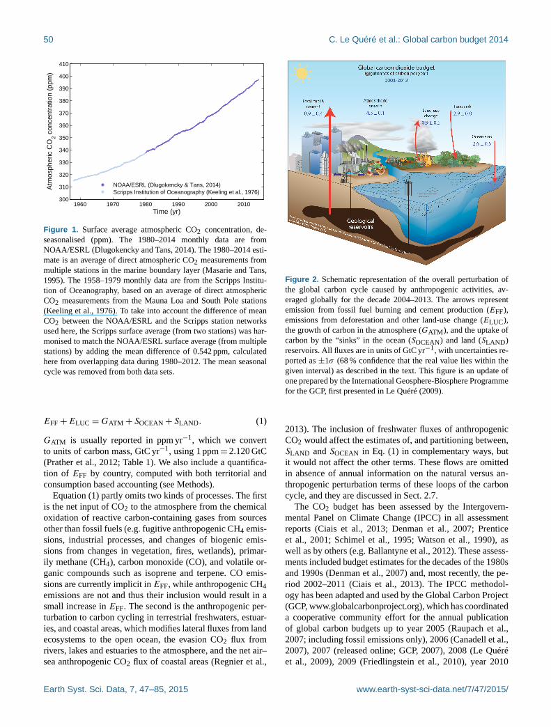
Figure 2. Schematic representation of the overall perturbation of
the global carbon cycle caused by anthropogenic activities, av-
eraged globally for the decade 2004–2013. The arrows represent
emission from fossil fuel burning and cement production (EFF),
emissions from deforestation and other land-use change (ELUC),
the growth of carbon in the atmosphere (GATM), and the uptake of
carbon by the “sinks” in the ocean (SOCEAN) and land (SLAND)
reservoirs. All fluxes are in units of GtC yr−1, with uncertainties re-
ported as ±1σ (68 % confidence that the real value lies within the
given interval) as described in the text. This figure is an update of
one prepared by the International Geosphere-Biosphere Programme
for the GCP, first presented in Le Quéré (2009).
2013). The inclusion of freshwater fluxes of anthropogenic
CO2 would affect the estimates of, and partitioning between,
SLAND and SOCEAN in Eq. (1) in complementary ways, but
it would not affect the other terms. These flows are omitted
in absence of annual information on the natural versus an-
thropogenic perturbation terms of these loops of the carbon
cycle, and they are discussed in Sect. 2.7.
The CO2 budget has been assessed by the Intergovern-
mental Panel on Climate Change (IPCC) in all assessment
reports (Ciais et al., 2013; Denman et al., 2007; Prentice
et al., 2001; Schimel et al., 1995; Watson et al., 1990), as
well as by others (e.g. Ballantyne et al., 2012). These assess-
ments included budget estimates for the decades of the 1980s
and 1990s (Denman et al., 2007) and, most recently, the pe-
riod 2002–2011 (Ciais et al., 2013). The IPCC methodol-
ogy has been adapted and used by the Global Carbon Project
(GCP, www.globalcarbonproject.org), which has coordinated
a cooperative community effort for the annual publication
of global carbon budgets up to year 2005 (Raupach et al.,
2007; including fossil emissions only), 2006 (Canadell et al.,
2007), 2007 (released online; GCP, 2007), 2008 (Le Quéré
et al., 2009), 2009 (Friedlingstein et al., 2010), year 2010
Earth Syst. Sci. Data, 7, 47–85, 2015 www.earth-syst-sci-data.net/7/47/2015/

C. Le Quéré et al.: Global carbon budget 2014 51
Table 1. Factors used to convert carbon in various units (by convention, Unit 1=Unit 2 · conversion).
Unit 1 Unit 2 Conversion Source
GtC (gigatonnes of carbon) ppm (parts per million) 2.120 Prather et al. (2012)
GtC (gigatonnes of carbon) PgC (petagrams of carbon) 1 SI unit conversion
GtCO2 (gigatonnes of carbon dioxide) GtC (gigatonnes of carbon) 3.664 44.01/12.011 in mass equivalent
GtC (gigatonnes of carbon) MtC (megatonnes of carbon) 1000 SI unit conversion
Table 2. How to cite the individual components of the global carbon budget presented here.
Component Primary reference
Territorial fossil fuel and cement emissions (EFF),
global, by fuel type, and by country
Boden et al. (2013; CDIAC:
http://cdiac.ornl.gov/trends/emis/meth_reg.html)
Consumption-based fossil fuel and cement emissions
(EFF) by country (consumption)
Peters et al. (2011b) updated as described in this paper
Land-use-change emissions (ELUC) Houghton et al. (2012) combined with Giglio et al.
(2013)
Atmospheric CO2 growth rate (GATM) Dlugokencky and Tans (2014; NOAA/ESRL:
www.esrl.noaa.gov/gmd/ccgg/trends/)
Ocean and land CO2 sinks (SOCEAN and SLAND) This paper for SOCEAN and SLAND and references in
Table 6 for individual models.
(Peters et al., 2012b), 2012 (Le Quéré et al., 2013; Peters et
al., 2013), and, most recently, 2013 (Le Quéré et al., 2014),
where the carbon budget year refers to the initial year of
publication. Each of these papers updated previous estimates
with the latest available information for the entire time series.
From 2008, these publications projected fossil fuel emissions
for one additional year using the projected world gross do-
mestic product (GDP) and estimated improvements in the
carbon intensity of the global economy.
We adopt a range of ±1 standard deviation (σ ) to report
the uncertainties in our estimates, representing a likelihood
of 68 % that the true value will be within the provided range
if the errors have a Gaussian distribution. This choice re-
flects the difficulty of characterising the uncertainty in the
CO2 fluxes between the atmosphere and the ocean and land
reservoirs individually, particularly on an annual basis, as
well as the difficulty of updating the CO2 emissions from
LUC. A likelihood of 68 % provides an indication of our
current capability to quantify each term and its uncertainty
given the available information. For comparison, the Fifth
Assessment Report of the IPCC (AR5) generally reported a
likelihood of 90 % for large data sets whose uncertainty is
well characterised, or for long time intervals less affected by
year-to-year variability. Our 68 % uncertainty value is near
the 66 % which the IPCC characterises as “likely” for values
falling into the±1σ interval. The uncertainties reported here
combine statistical analysis of the underlying data and ex-
pert judgement of the likelihood of results lying outside this
range. The limitations of current information are discussed
in the paper.
All quantities are presented in units of gigatonnes of car-
bon (GtC, 1015 gC), which is the same as petagrams of car-
bon (PgC; Table 1). Units of gigatonnes of CO2 (or billion
tonnes of CO2) used in policy are equal to 3.664 multiplied
by the value in units of GtC.
This paper provides a detailed description of the data sets
and methodology used to compute the global carbon bud-
get estimates for the period pre-industrial (1750) to 2013 and
in more detail for the period 1959 to 2013. We also pro-
vide decadal averages starting in 1960 and including the last
decade (2004–2013), results for the year 2013, and a pro-
jection of EFF for year 2014. Finally, we provide the to-
tal or cumulative emissions from fossil fuels and land-use
change since the year 1750; the pre-industrial period; and
since year 1870, the reference year for the cumulative car-
bon estimate used by the IPCC (AR5) based on the availabil-
ity of global temperature data (Stocker et al., 2013b). This
paper will be updated every year using the format of “liv-
ing data” so as to keep a record of budget versions and the
changes in new data, revision of data, and changes in method-
ology that lead to changes in estimates of the carbon budget.
Additional materials associated with the release of each new
version will be posted on the Global Carbon Project (GCP)
website (http://www.globalcarbonproject.org/carbonbudget).
Data associated with this release are also available through
the Global Carbon Atlas (http://www.globalcarbonatlas.org).
With this approach, we aim to provide the highest trans-
www.earth-syst-sci-data.net/7/47/2015/ Earth Syst. Sci. Data, 7, 47–85, 2015

52 C. Le Quéré et al.: Global carbon budget 2014
parency and traceability in the reporting of key indicators and
drivers of climate change.
2 Methods
Multiple organisations and research groups around the world
generated the original measurements and data used to com-
plete the global carbon budget. The effort presented here is
thus mainly one of synthesis, where results from individual
groups are collated, analysed, and evaluated for consistency.
We facilitate access to original data with the understand-
ing that primary data sets will be referenced in future work
(see Table 2 for how to cite the data sets). Descriptions of
the measurements, models, and methodologies follow below,
and in-depth descriptions of each component are described
elsewhere (e.g. Andres et al., 2012; Houghton et al., 2012).
This is the ninth version of the “global carbon budget” (see
Introduction for details) and the third revised version of the
“global carbon budget living data paper”. It is an update of
Le Quéré et al. (2014), including data to year 2013 (inclu-
sive) and a projection for fossil fuel emissions for year 2014.
The main changes from Le Quéré et al. (2014) are as fol-
lows: (1) we use 3 years of BP energy consumption growth
rates (coal, oil, gas) to estimate EFF compared to 2 years
in the previous version (Sect. 2.1), (2) we updated SOCEAN
estimates from observations to 2013 extending the Surface
Ocean CO2 Atlas (SOCAT) v2 database (Bakker et al., 2014;
Sect. 2.4) with additional new cruises, and (3) we introduced
results from three atmospheric inverse methods using atmo-
spheric measurements from a global network of surface sta-
tions through 2013 that provide a latitudinal breakdown of
the combined land and ocean fluxes (Sect. 2.6). The main
methodological differences between annual carbon budgets
are summarised in Table 3.
2.1 CO2 emissions from fossil fuel combustion and
cement production (EFF)
2.1.1 Fossil fuel and cement emissions and their
uncertainty
The calculation of global and national CO2 emissions from
fossil fuel combustion, including gas flaring and cement pro-
duction (EFF), relies primarily on energy consumption data,
specifically data on hydrocarbon fuels, collated and archived
by several organisations (Andres et al., 2012). These include
the Carbon Dioxide Information Analysis Center (CDIAC),
the International Energy Agency (IEA), the United Nations
(UN), the United States Department of Energy (DoE) En-
ergy Information Administration (EIA), and more recently
also the Planbureau voor de Leefomgeving (PBL) of the
Netherlands Environmental Assessment Agency. We use the
emissions estimated by the CDIAC (Boden et al., 2013).
The CDIAC emission estimates constitute the only data set
that extends back in time to 1751 with consistent and well-
documented emissions from fossil fuel combustion, cement
production, and gas flaring for all countries and their uncer-
tainty (Andres et al., 1999, 2012, 2014); this makes the data
set a unique resource for research of the carbon cycle during
the fossil fuel era.
During the period 1959–2010, the emissions from fossil
fuel consumption are based primarily on energy data pro-
vided by the UN Statistics Division (Table 4; UN, 2013a, b).
When necessary, fuel masses/volumes are converted to fuel
energy content using coefficients provided by the UN and
then to CO2 emissions using conversion factors that take into
account the relationship between carbon content and energy
(heat) content of the different fuel types (coal, oil, gas, gas
flaring) and the combustion efficiency (to account, for exam-
ple, for soot left in the combustor or fuel otherwise lost or dis-
charged without oxidation). Most data on energy consump-
tion and fuel quality (carbon content and heat content) are
available at the country level (UN, 2013a). In general, CO2
emissions for equivalent primary energy consumption are
about 30 % higher for coal compared to oil, and 70 % higher
for coal compared to natural gas (Marland et al., 2007). All
estimated fossil fuel emissions are based on the mass flows
of carbon and assume that the fossil carbon emitted as CO or
CH4 will soon be oxidised to CO2 in the atmosphere and can
be accounted for with CO2 emissions (see Sect. 2.7).
For the three most recent years (2011, 2012, and 2013)
when the UN statistics are not yet available, we generated
preliminary estimates based on the BP annual energy review
by applying the growth rates of energy consumption (coal,
oil, gas) for 2011–2013 (BP, 2014) to the CDIAC emissions
in 2010. BP’s sources for energy statistics overlap with those
of the UN data but are compiled more rapidly from about 70
countries covering about 96 % of global emissions. We use
the BP values only for the year-to-year rate of change, be-
cause the rates of change are less uncertain than the absolute
values and to avoid discontinuities in the time series when
linking the UN-based energy data (up to 2010) with the BP
energy data (2011–2013). These preliminary estimates are
replaced with the more complete CDIAC data based on UN
statistics when they become available. Past experience and
work by others (Andres et al., 2014) shows that projections
based on the BP rate of change are within the uncertainty
provided (see Sect. 3.2 and Supplement from Peters et al.,
2013).
Emissions from cement production are based on cement
production data from the U.S. Geological Survey up to year
2012 (van Oss, 2013), and up to 2013 for the top 18 countries
(representing 85 % of global production; USGS, 2014). For
countries without data in 2013 we use the 2012 values (zero
growth). Some fraction of the CaO and MgO in cement is
returned to the carbonate form during cement weathering, but
this is generally regarded to be small and is ignored here.
Emission estimates from gas flaring are calculated in a
similar manner as those from solid, liquid, and gaseous fuels,
and rely on the UN Energy Statistics to supply the amount
Earth Syst. Sci. Data, 7, 47–85, 2015 www.earth-syst-sci-data.net/7/47/2015/
C. Le Quéré et al.: Global carbon budget 2014 53
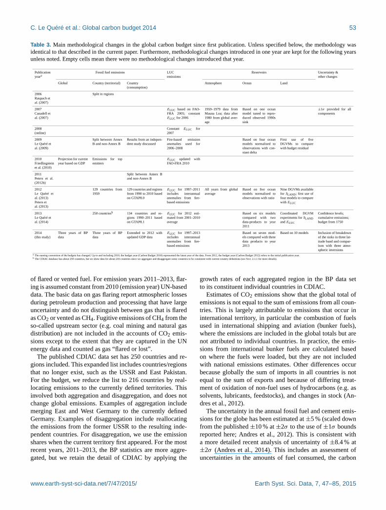
Table 3. Main methodological changes in the global carbon budget since first publication. Unless specified below, the methodology was
identical to that described in the current paper. Furthermore, methodological changes introduced in one year are kept for the following years
unless noted. Empty cells mean there were no methodological changes introduced that year.
Publication
yearaFossil fuel emissions LUC
emissions
Reservoirs Uncertainty &
other changes
Global Country (territorial) Country
(consumption)
Atmosphere Ocean Land
2006
Raupach et
al. (2007)
Split in regions
2007
Canadell et
al. (2007)
ELUC based on FAO-
FRA 2005; constant
ELUC for 2006
1959–1979 data from
Mauna Loa; data after
1980 from global aver-
age
Based on one ocean
model tuned to repro-
duced observed 1990s
sink
±1σ provided for all
components
2008
(online)
Constant ELUC for
2007
2009
Le Quéré et
al. (2009)
Split between Annex
B and non-Annex B
Results from an indepen-
dent study discussed
Fire-based emission
anomalies used for
2006–2008
Based on four ocean
models normalised to
observations with con-
stant delta
First use of five
DGVMs to compare
with budget residual
2010
Friedlingstein
et al. (2010)
Projection for current
year based on GDP
Emissions for top
emitters
ELUC updated with
FAO-FRA 2010
2011
Peters et al.
(2012b)
Split between Annex B
and non-Annex B
2012
Le Quéré et
al. (2013)
Peters et
al. (2013)
129 countries from
1959
129 countries and regions
from 1990 to 2010 based
on GTAP8.0
ELUC for 1997–2011
includes interannual
anomalies from fire-
based emissions
All years from global
average
Based on five ocean
models normalised to
observations with ratio
Nine DGVMs available
for SLAND; first use of
four models to compare
with ELUC
2013
Le Quéré et
al. (2014)
250 countriesb 134 countries and re-
gions 1990–2011 based
on GTAP8.1
ELUC for 2012 esti-
mated from 2001–2010
average
Based on six models
compared with two
data-products to year
2011
Coordinated DGVM
experiments for SLAND
and ELUC
Confidence levels;
cumulative emissions;
budget from 1750
2014
(this study)
Three years of BP
data
Three years of BP
data
Extended to 2012 with
updated GDP data
ELUC for 1997–2013
includes interannual
anomalies from fire-
based emissions
Based on seven mod-
els compared with three
data products to year
2013
Based on 10 models Inclusion of breakdown
of the sinks in three lat-
itude band and compar-
ison with three atmo-
spheric inversions
a The naming convention of the budgets has changed. Up to and including 2010, the budget year (Carbon Budget 2010) represented the latest year of the data. From 2012, the budget year (Carbon Budget 2012) refers to the initial publication year.b The CDIAC database has about 250 countries, but we show data for about 216 countries since we aggregate and disaggregate some countries to be consistent with current country definitions (see Sect. 2.1.1 for more details).
of flared or vented fuel. For emission years 2011–2013, flar-
ing is assumed constant from 2010 (emission year) UN-based
data. The basic data on gas flaring report atmospheric losses
during petroleum production and processing that have large
uncertainty and do not distinguish between gas that is flared
as CO2 or vented as CH4. Fugitive emissions of CH4 from the
so-called upstream sector (e.g. coal mining and natural gas
distribution) are not included in the accounts of CO2 emis-
sions except to the extent that they are captured in the UN
energy data and counted as gas “flared or lost”.
The published CDIAC data set has 250 countries and re-
gions included. This expanded list includes countries/regions
that no longer exist, such as the USSR and East Pakistan.
For the budget, we reduce the list to 216 countries by real-
locating emissions to the currently defined territories. This
involved both aggregation and disaggregation, and does not
change global emissions. Examples of aggregation include
merging East and West Germany to the currently defined
Germany. Examples of disaggregation include reallocating
the emissions from the former USSR to the resulting inde-
pendent countries. For disaggregation, we use the emission
shares when the current territory first appeared. For the most
recent years, 2011–2013, the BP statistics are more aggre-
gated, but we retain the detail of CDIAC by applying the
growth rates of each aggregated region in the BP data set
to its constituent individual countries in CDIAC.
Estimates of CO2 emissions show that the global total of
emissions is not equal to the sum of emissions from all coun-
tries. This is largely attributable to emissions that occur in
international territory, in particular the combustion of fuels
used in international shipping and aviation (bunker fuels),
where the emissions are included in the global totals but are
not attributed to individual countries. In practice, the emis-
sions from international bunker fuels are calculated based
on where the fuels were loaded, but they are not included
with national emissions estimates. Other differences occur
because globally the sum of imports in all countries is not
equal to the sum of exports and because of differing treat-
ment of oxidation of non-fuel uses of hydrocarbons (e.g. as
solvents, lubricants, feedstocks), and changes in stock (An-
dres et al., 2012).
The uncertainty in the annual fossil fuel and cement emis-
sions for the globe has been estimated at ±5 % (scaled down
from the published ±10 % at ±2σ to the use of ±1σ bounds
reported here; Andres et al., 2012). This is consistent with
a more detailed recent analysis of uncertainty of ±8.4 % at
±2σ (Andres et al., 2014). This includes an assessment of
uncertainties in the amounts of fuel consumed, the carbon
www.earth-syst-sci-data.net/7/47/2015/ Earth Syst. Sci. Data, 7, 47–85, 2015

54 C. Le Quéré et al.: Global carbon budget 2014
Table 4. Data sources used to compute each component of the global carbon budget.
Component Process Data source Data reference
EFF Fossil fuel combustion and gas flaring UN Statistics Division to 2010 UN (2013a, b)
BP for 2011–2013 BP (2014)
Cement production U.S. Geological Survey van Oss (2013)
U.S. Geological Survey (2012)
ELUC Land-cover change (deforestation, afforesta-
tion, and forest regrowth)
Forest Resource Assessment (FRA) of the Food
and Agriculture Organization (FAO)
FAO (2010)
Wood harvest FAO Statistics Division FAOSTAT (2010)
Shifting agriculture FAO FRA and Statistics Division FAO (2010), FAOSTAT (2010)
Interannual variability from peat fires and
climate–land management interactions (1997–
2013)
Global Fire Emissions Database (GFED4) Giglio et al. (2013)
GATM Change in atmospheric CO2 concentration 1959–1980: CO2 Program at Scripps Institution
of Oceanography and other research groups
Keeling et al. (1976)
1980–2013: US National Oceanic and Atmo-
spheric Administration Earth System Research
Laboratory
Dlugokencky and Tans (2014)
Ballantyne et al. (2012)
SOCEAN Uptake of anthropogenic CO2 1990–1999 average: indirect estimates based on
CFCs, atmospheric O2, and other tracer obser-
vations
Manning and Keeling (2006)
Keeling et al. (2011)
McNeil et al. (2003)
Mikaloff Fletcher et al. (2006) as assessed
by the IPCC
Denman et al. (2007)
Impact of increasing atmospheric CO2, climate
and variability
Ocean models Table 6
SLAND Response of land vegetation to
increasing atmospheric CO2 concentration,
climate and variability and
other environmental changes
Budget residual
and heat contents of fuels, and the combustion efficiency.
While in the budget we consider a fixed uncertainty of ±5 %
for all years, in reality the uncertainty, as a percentage of the
emissions, is growing with time because of the larger share
of global emissions from non-Annex B countries (emerging
economies and developing countries) with less precise sta-
tistical systems (Marland et al., 2009). For example, the un-
certainty in Chinese emissions has been estimated at around
±10 % (for ±1σ ; Gregg et al., 2008). Generally, emissions
from mature economies with good statistical bases have an
uncertainty of only a few percent (Marland, 2008). Further
research is needed before we can quantify the time evolu-
tion of the uncertainty, and its temporal error correlation
structure. We note that, even if they are presented as 1σ es-
timates, uncertainties of emissions are likely to be mainly
country-specific systematic errors related to underlying bi-
ases of energy statistics and to the accounting method used
by each country. We assign a medium confidence to the re-
sults presented here because they are based on indirect esti-
mates of emissions using energy data (Durant et al., 2010).
There is only limited and indirect evidence for emissions,
although there is a high agreement among the available es-
timates within the given uncertainty (Andres et al., 2012,
2014), and emission estimates are consistent with a range of
other observations (Ciais et al., 2013), even though their re-
gional and national partitioning is more uncertain (Francey
et al., 2013).
2.1.2 Emissions embodied in goods and services
National emission inventories take a territorial (production)
perspective and “include greenhouse gas emissions and re-
movals taking place within national territory and offshore
areas over which the country has jurisdiction” (Rypdal et
al., 2006). That is, emissions are allocated to the country
where and when the emissions actually occur. The territo-
rial emission inventory of an individual country does not in-
clude the emissions from the production of goods and ser-
vices produced in other countries (e.g. food and clothes)
that are used for consumption. Consumption-based emission
inventories for an individual country is another attribution
point of view that allocates global emissions to products that
are consumed within a country, and are conceptually cal-
culated as the territorial emissions minus the “embedded”
territorial emissions to produce exported products plus the
emissions in other countries to produce imported products
(consumption= territorial− exports+ imports). The differ-
ence between the territorial- and consumption-based emis-
sion inventories is the net transfer (exports minus imports) of
emissions from the production of internationally traded prod-
ucts. Consumption-based emission attribution results (e.g.
Earth Syst. Sci. Data, 7, 47–85, 2015 www.earth-syst-sci-data.net/7/47/2015/

C. Le Quéré et al.: Global carbon budget 2014 55
Davis and Caldeira, 2010) provide additional information
on territorial-based emissions that can be used to under-
stand emission drivers (Hertwich and Peters, 2009), quantify
emission (virtual) transfers by the trade of products between
countries (Peters et al., 2011b), and potentially design more
effective and efficient climate policy (Peters and Hertwich,
2008).
We estimate consumption-based emissions by enumerat-
ing the global supply chain using a global model of the eco-
nomic relationships between economic sectors within and
between every country (Andrew and Peters, 2013; Peters et
al., 2011a). Due to availability of the input data, detailed es-
timates are made for the years 1997, 2001, 2004, and 2007
(using the methodology of Peters et al., 2011b) using eco-
nomic and trade data from the Global Trade and Analysis
Project version 8.1 (GTAP; Narayanan et al., 2013). The re-
sults cover 57 sectors and 134 countries and regions. The
results are extended into an annual time series from 1990 to
the latest year of the fossil fuel emissions or GDP data (2012
in this budget), using GDP data by expenditure in current ex-
change rate of US dollars (USD; from the UN National Ac-
counts Main Aggregates database; UN, 2014) and time series
of trade data from GTAP (based on the methodology in Pe-
ters et al., 2011b).
The consumption-based emission inventories in this car-
bon budget incorporate several improvements over previous
versions (Le Quéré et al., 2013; Peters et al., 2011b, 2012b).
The detailed estimates for 2004 and 2007 and time series ap-
proximation from 1990 to 2012 are based on an updated ver-
sion of the GTAP database (Narayanan et al., 2013). We es-
timate the sector level CO2 emissions using our own calcula-
tions based on the GTAP data and methodology, include flar-
ing and cement emissions from CDIAC, and then scale the
national totals (excluding bunker fuels) to match the CDIAC
estimates from the most recent carbon budget. We do not in-
clude international transportation in our estimates of national
totals, but we do include them in the global total. The time se-
ries of trade data provided by GTAP covers the period 1995–
2009 and our methodology uses the trade shares as this data
set. For the period 1990–1994 we assume the trade shares of
1995, while for 2010 and 2011 we assume the trade shares of
2008 since 2009 was heavily affected by the global financial
crisis. We identified errors in the trade shares of Taiwan in
2008 and 2009, so its trade shares for 2008–2010 are based
on the 2007 trade shares.
We do not provide an uncertainty estimate for these emis-
sions, but based on model comparisons and sensitivity analy-
sis, they are unlikely to be larger than for the territorial emis-
sion estimates (Peters et al., 2012a). Uncertainty is expected
to increase for more detailed results and decrease with ag-
gregation (Peters et al., 2011b; e.g. the results for Annex B
countries will be more accurate than the sector results for an
individual country).
The consumption-based emissions attribution method con-
siders the CO2 emitted to the atmosphere in the production
of products, but not the trade in fossil fuels (coal, oil, gas).
It is also possible to account for the carbon trade in fossil
fuels (Davis et al., 2011), but we do not present those data
here. Peters et al. (2012a) additionally considered trade in
biomass.
The consumption data do not modify the global average
terms in Eq. (1), but they are relevant to the anthropogenic
carbon cycle as they reflect the trade-driven movement of
emissions across the Earth’s surface in response to human
activities. Furthermore, if national and international climate
policies continue to develop in an unharmonised way, then
the trends reflected in these data will need to be accommo-
dated by those developing policies.
2.1.3 Growth rate in emissions
We report the annual growth rate in emissions for adjacent
years (in percent per year) by calculating the difference be-
tween the 2 years and then comparing to the emissions in the
first year:
[E
FF(t0+1)−EFF(t0)
EFF(t0)
]×% yr−1. This is the simplest
method to characterise a 1-year growth compared to the pre-
vious year and is widely used. We apply a leap-year adjust-
ment to ensure valid interpretations of annual growth rates.
This affects the growth rate by about 0.3 % yr−1 ( 1365
) and
causes growth rates to go up approximately 0.3 % if the first
year is a leap year and down 0.3 % if the second year is a leap
year.
The relative growth rate of EFF over time periods of
greater than 1 year can be re-written using its logarithm
equivalent as follows:
1
EFF
dEFF
dt=
d(lnEFF)
dt. (2)
Here we calculate relative growth rates in emissions for
multi-year periods (e.g. a decade) by fitting a linear trend
to ln(EFF) in Eq. (2), reported in percent per year. We fit
the logarithm of EFF rather than EFF directly because this
method ensures that computed growth rates satisfy Eq. (6).
This method differs from previous papers (Canadell et al.,
2007; Le Quéré et al., 2009; Raupach et al., 2007) that com-
puted the fit to EFF and divided by average EFF directly, but
the difference is very small (< 0.05 %) in the case of EFF.
2.1.4 Emissions projections using GDP projections
Energy statistics are normally available around June for the
previous year. We use the close relationship between the
growth in world GDP and the growth in global emissions
(Raupach et al., 2007) to project emissions for the current
year. This is based on the so-called Kaya identity (also
called IPAT identity, the acronym standing for human im-
pact (I) on the environment, which is equal to the prod-
uct of population (P), affluence (A), and technology (T),
whereby EFF (GtC yr−1) is decomposed by the product of
www.earth-syst-sci-data.net/7/47/2015/ Earth Syst. Sci. Data, 7, 47–85, 2015

56 C. Le Quéré et al.: Global carbon budget 2014
GDP (USD yr−1) and the fossil fuel carbon intensity of the
economy (IFF; GtC USD−1) as follows:
EFF = GDP× IFF. (3)
Such product-rule decomposition identities imply that the
relative growth rates of the multiplied quantities are additive.
Taking a time derivative of Eq. (3) gives
dEFF
dt=
d(GDP× IFF)
dt, (4)
and, applying the rules of calculus,
dEFF
dt=
dGDP
dt× IFF+GDP×
dIFF
dt; (5)
finally, dividing Eq. (5) by Eq. (3) gives
1
EFF
dEFF
dt=
1
GDP
dGDP
dt+
1
IFF
dIFF
dt, (6)
where the left-hand term is the relative growth rate of EFF,
and the right-hand terms are the relative growth rates of GDP
and IFF, respectively, which can simply be added linearly to
give overall growth rate. The growth rates are reported in per-
cent by multiplying each term by 100. As preliminary esti-
mates of annual change in GDP are made well before the end
of a calendar year, making assumptions on the growth rate of
IFF allows us to make projections of the annual change in
CO2 emissions well before the end of a calendar year.
2.2 CO2 emissions from land use, land-use change,
and forestry (ELUC)
LUC emissions reported in the 2014 carbon budget (ELUC)
include CO2 fluxes from deforestation, afforestation, log-
ging (forest degradation and harvest activity), shifting culti-
vation (cycle of cutting forest for agriculture and then aban-
doning), and regrowth of forests following wood harvest or
abandonment of agriculture. Only some land management
activities (Table 5) are included in our LUC emissions es-
timates (e.g. emissions or sinks related to management and
management changes in established pasture and croplands
are not included). Some of these activities lead to emissions
of CO2 to the atmosphere, while others lead to CO2 sinks.
ELUC is the net sum of all anthropogenic activities consid-
ered. Our annual estimate for 1959–2010 is from a book-
keeping method (Sect. 2.2.1) primarily based on net forest
area change and biomass data from the Forest Resource As-
sessment (FRA) of the Food and Agriculture Organization
(FAO), which is only available at intervals of 5 years and
ends in 2010 (Houghton et al., 2012). Interannual variabil-
ity in emissions due to deforestation and degradation have
been coarsely estimated from satellite-based fire activity in
tropical forest areas (Sect. 2.2.2; Giglio et al., 2013; van
der Werf et al., 2010). The bookkeeping method is used to
quantify the ELUC over the time period of the available data,
and the satellite-based deforestation fire information to incor-
porate interannual variability (ELUC flux annual anomalies)
from tropical deforestation fires. The satellite-based defor-
estation and degradation fire emissions estimates are avail-
able for years 1997–2013. We calculate the global annual
anomaly in deforestation and degradation fire emissions in
tropical forest regions for each year, compared to the 1997–
2010 period, and add this annual flux anomaly to the ELUC
estimated using the bookkeeping method that is available up
to 2010 only and assumed constant at the 2010 value during
the period 2011–2013. We thus assume that all land manage-
ment activities apart from deforestation and degradation do
not vary significantly on a year-to-year basis. Other sources
of interannual variability (e.g. the impact of climate variabil-
ity on regrowth fluxes) are accounted for in SLAND. In ad-
dition, we use results from dynamic global vegetation mod-
els (see Sect. 2.2.3 and Table 6) that calculate net LUC CO2
emissions in response to land-cover-change reconstructions
prescribed to each model in order to help quantify the uncer-
tainty in ELUC and to explore the consistency of our under-
standing. The three methods are described below, and differ-
ences are discussed in Sect. 3.2.
2.2.1 Bookkeeping method
LUC CO2 emissions are calculated by a bookkeeping method
approach (Houghton, 2003) that keeps track of the carbon
stored in vegetation and soils before deforestation or other
land-use change, and the changes in forest age classes, or
cohorts, of disturbed lands after land-use change including
possible forest regrowth after deforestation. It tracks the CO2
emitted to the atmosphere immediately during deforestation,
and over time due to the follow-up decay of soil and vegeta-
tion carbon in different pools, including wood product pools
after logging and deforestation. It also tracks the regrowth of
vegetation and associated build-up of soil carbon pools after
LUC. It considers transitions between forests, pastures, and
cropland; shifting cultivation; degradation of forests where a
fraction of the trees is removed; abandonment of agricultural
land; and forest management such as wood harvest and, in
the USA, fire management. In addition to tracking logging
debris on the forest floor, the bookkeeping method tracks the
fate of carbon contained in harvested wood products that is
eventually emitted back to the atmosphere as CO2, although
a detailed treatment of the lifetime in each product pool is not
performed (Earles et al., 2012). Harvested wood products are
partitioned into three pools with different turnover times. All
fuel wood is assumed burned in the year of harvest (1.0 yr−1).
Pulp and paper products are oxidised at a rate of 0.1 yr−1,
timber is assumed to be oxidised at a rate of 0.01 yr−1, and
elemental carbon decays at 0.001 yr−1. The general assump-
tions about partitioning wood products among these pools
are based on national harvest data (Houghton, 2003).
The primary land-cover-change and biomass data for the
bookkeeping method analysis are from the Forest Resource
Earth Syst. Sci. Data, 7, 47–85, 2015 www.earth-syst-sci-data.net/7/47/2015/

C. Le Quéré et al.: Global carbon budget 2014 57
Table 5. Comparison of the processes included in the ELUC of the global carbon budget and the DGVMs. See Table 6 for model references.
All models include deforestation and forest regrowth after abandonment of agriculture (or from afforestation activities on agricultural land).
Bo
ok
kee
pin
g
CA
BL
E
CL
M4
.5B
GC
ISA
M
JUL
ES
LP
J-G
UE
SS
LP
J
LP
X
OR
CH
IDE
E
VE
GA
S
VIS
IT
Wood harvest and for-
est degradationayes yes yes yes no no no no no yes yesb
Shifting cultivation yes no yes no no no no no noc nod yes
Cropland harvest yes yes yes no no yes no yes yes yes yes
Peat fires no no yes no no no no no no no no
Fire simulation and/or
suppression
for US only no yes no no yes yes yes no yes yes
Climate and variability no yes yes yes yes yes yes yes yes yes yes
CO2 fertilisation no yes yes yes yes yes yes yes yes yes yes
Carbon–nitrogen
interactions, including
N deposition
no yes yes yes no no no yes no no no
a Refers to the routine harvest of established managed forests rather than pools of harvested products. b Wood stems are harvested according to
the land-use data. c Models only used to calculate SLAND. d Model only used to compare ELUC + SLAND to atmospheric inversions (Fig. 6).
Assessment of the FAO, which provides statistics on forest-
cover change and management at intervals of 5 years (FAO,
2010). The data are based on countries’ self-reporting, some
of which includes satellite data in more recent assessments
(Table 4). Changes in land cover other than forest are based
on annual, national changes in cropland and pasture areas
reported by the FAO Statistics Division (FAOSTAT, 2010).
LUC country data are aggregated by regions. The carbon
stocks on land (biomass and soils), and their response func-
tions subsequent to LUC, are based on FAO data averages
per land-cover type, biome, and region. Similar results were
obtained using forest biomass carbon density based on satel-
lite data (Baccini et al., 2012). The bookkeeping method does
not include land ecosystems’ transient response to changes in
climate, atmospheric CO2, and other environmental factors,
but the growth/decay curves are based on contemporary data
that will implicitly reflect the effects of CO2 and climate at
that time. Results from the bookkeeping method are available
from 1850 to 2010.
2.2.2 Fire-based method
LUC-associated CO2 emissions calculated from satellite-
based fire activity in tropical forest areas (van der Werf et
al., 2010) provide information on emissions due to tropical
deforestation and degradation that are complementary to the
bookkeeping approach. They do not provide a direct estimate
of ELUC as they do not include non-combustion processes
such as respiration, wood harvest, wood products, and forest
regrowth. Legacy emissions such as decomposition from on-
ground debris and soils are not included in this method either.
However, fire estimates provide some insight into the year-to-
year variations in the sub-component of the total ELUC flux
that result from immediate CO2 emissions during deforesta-
tion caused, for example, by the interactions between climate
and human activity (e.g. there is more burning and clearing of
forests in dry years) that are not represented by other meth-
ods. The “deforestation fire emissions” assume an important
role of fire in removing biomass in the deforestation process,
and thus can be used to infer gross instantaneous CO2 emis-
sions from deforestation using satellite-derived data on fire
activity in regions with active deforestation. The method re-
quires information on the fraction of total area burned as-
sociated with deforestation versus other types of fires, and
this information can be merged with information on biomass
stocks and the fraction of the biomass lost in a deforestation
fire to estimate CO2 emissions. The satellite-based deforesta-
tion fire emissions are limited to the tropics, where fires re-
sult mainly from human activities. Tropical deforestation is
the largest and most variable single contributor to ELUC.
Fire emissions associated with deforestation and tropi-
cal peat burning are based on the Global Fire Emissions
Database (GFED) described in van der Werf et al. (2010)
but with updated burned area (Giglio et al., 2013) as well
as burned area from relatively small fires that are detected by
satellite as thermal anomalies but not mapped by the burned-
area approach (Randerson et al., 2012). The burned-area in-
formation is used as input data in a modified version of the
satellite-driven Carnegie–Ames–Stanford Approach (CASA)
biogeochemical model to estimate carbon emissions associ-
ated with fires, keeping track of what fraction of fire emis-
sions was due to deforestation (see van der Werf et al., 2010).
The CASA model uses different assumptions to compute
www.earth-syst-sci-data.net/7/47/2015/ Earth Syst. Sci. Data, 7, 47–85, 2015

58 C. Le Quéré et al.: Global carbon budget 2014
Table 6. References for the process models and data products included in Figs. 6–8.
Model/data
name
Reference Change from Le Quéré et al. (2013)
Dynamic global vegetation models
CABLE2.0 Zhang et al. (2013) Updated model from CABLE1.4 (Wang et al., 2011) to include full carbon, nitrogen, and phos-
phorus cycle (Wang et al., 2010) and land cover and land-cover change.
CLM4.5BGCa Oleson et al. (2013) Updated model from CLM4.0CN to CLM4.5BGC. Major changes include revised photosynthe-
sis, slower turnover times for decomposition of litter and SOM, vertically resolved soil biogeo-
chemistry, revised soil denitrification and nitrification, new fire model, and revised frozen-soil
hydrology. As shown in Koven et al. (2013), these changes collectively bring model into better
agreement with 20th century C budget.
ISAM Jain et al. (2013)b Not applicable
JULESc Clark et al. (2011)d Updated model from JULESv1 (Cox et al., 2000) to JULESv3.2 as configured in the latest
generation ESM-HadGEM2-ES (Collins et al., 2011). Higher resolution (1.875× 1.25) and with
an improved snow scheme, multi-pool soil carbon model, updated representation of land-use
change.
LPJ-GUESS Smith et al. (2001) Not applicable
LPJe Sitch et al. (2003) Decreased LPJ wood harvest efficiency so that 50 % of biomass was removed off-site compared
to 85 % used in the 2012 budget. Residue management of managed grasslands increased so that
100 % of harvested grass enters litter pool.
LPX Stocker et al. (2013a) Addition of C–N cycle coupling.
ORCHIDEE Krinner et al. (2005) Revised parameters values for photosynthetic capacity for boreal forests (following assimilation
of FLUXNET data), updated parameters values for stem allocation, maintenance respiration
and biomass export for tropical forests (based on literature), and CO2 down-regulation process
added to photosynthesis.
VEGAS Zeng et al. (2005)f Improved wetland and permafrost parameterisations, high-latitude temperature dependence
VISIT Kato et al. (2013)g Wood harvest flux is added to ELUC, and the loss of additional sink capacity is also included in
the ELUC due to the methodological change of using coordinated DGVM experiments.
Data products for land-use-change emissions
Bookkeeping Houghton et al. (2012) No change
Fire-based
emissions
van der Werf et al. (2010) No change
Ocean biogeochemistry models
NEMO-
PlankTOM5
Buitenhuis et al. (2010)h No change
NEMO-
PISCES
(IPSL)i
Aumont and Bopp (2006) No change
CCSM-BEC Doney et al. (2009) No change
MICOM-
HAMOCC
Assmann et al. (2010)j No change
MPIOM-
HAMOCC
Ilyina et al. (2013) No change
NEMO-
PISCES
(CNRM)
Séférian et al. (2013)k Not applicable
CSIRO Oke et al. (2013) Not applicable
Data products for ocean CO2 sink
Landschützer Landschützer et al. (2014) Not applicable
Park Park et al. (2010)l No change
Rödenbeck Rödenbeck et al. (2014)m No change
Atmospheric inversions for total CO2 fluxes (land-use change+ land+ ocean CO2 sinks)
Peters Peters et al. (2010) Not applicable
Rödenbeck Rödenbeck et al. (2003) Not applicable
MACCn Chevallier et al. (2005) Not applicable
a Community Land Model 4.5. b See also El-Masri et al. (2013). c Joint UK Land Environment Simulator. d See also Best et al. (2011) e Lund–Potsdam–Jena. f Only used for total land
(ELUC+SLAND) flux calculation of multi-model mean. g See also Ito and Inatomi (2012). h With no nutrient restoring below the mixed layer depth. i Referred to as LSCE in previous carbon
budgets. j With updates to the physical model as described in Tjiputra et al. (2013). k Further information (e.g. physical evaluation) for CNRM model can be found in Danabasoglu et
al. (2014). l Using winds from Atlas et al. (2011). m Updated version “s81_v3.6gcp”. n The MACC v13.1 CO2 inversion system, initially described by Chevallier et al. (2005), relies on the
global tracer transport model LMDZ (Hourdin et al., 2006; see also Supplement to Peylin et al., 2013).
Earth Syst. Sci. Data, 7, 47–85, 2015 www.earth-syst-sci-data.net/7/47/2015/

C. Le Quéré et al.: Global carbon budget 2014 59
decay functions compared to the bookkeeping method, and
does not include historical emissions or regrowth from land-
use change prior to the availability of satellite data. Compar-
ing coincident CO emissions and their atmospheric fate with
satellite-derived CO concentrations allows for some valida-
tion of this approach (e.g. van der Werf et al., 2008). Re-
sults from the fire-based method to estimate LUC emissions
anomalies added to the bookkeeping meanELUC estimate are
available from 1997 to 2013. Our combination of LUC CO2
emissions where the variability of annual CO2 deforestation
emissions is diagnosed from fires assumes that year-to-year
variability is dominated by variability in deforestation.
2.2.3 Dynamic global vegetation models (DGVMs)
LUC CO2 emissions have been estimated using an ensem-
ble of seven DGVMs. New model experiments up to year
2013 have been coordinated by the project “Trends and
drivers of the regional-scale sources and sinks of carbon
dioxide” (TRENDY; http://dgvm.ceh.ac.uk/node/9). We use
only models that have estimated LUC CO2 emissions and
the terrestrial residual sink following the TRENDY protocol
(see Sect. 2.5.2), thus providing better consistency in the as-
sessment of the causes of carbon fluxes on land. Models use
their latest configurations, summarised in Tables 5 and 6.
The DGVMs were forced with historical changes in land-
cover distribution, climate, atmospheric CO2 concentration,
and N deposition. As further described below, each histor-
ical DGVM simulation was repeated with a time-invariant
pre-industrial land-cover distribution, allowing for estima-
tion of, by difference with the first simulation, the dynamic
evolution of biomass and soil carbon pools in response to
prescribed land-cover change. All DGVMs represent defor-
estation and (to some extent) regrowth, the most important
components of ELUC, but they do not represent all processes
resulting directly from human activities on land (Table 5).
DGVMs represent processes of vegetation growth and mor-
tality, as well as decomposition of dead organic matter asso-
ciated with natural cycles, and include the vegetation and soil
carbon response to increasing atmospheric CO2 levels and to
climate variability and change. In addition, four models ex-
plicitly simulate the coupling of C and N cycles and account
for atmospheric N deposition (Table 5). The DGVMs are in-
dependent of the other budget terms except for their use of
atmospheric CO2 concentration to calculate the fertilisation
effect of CO2 on primary production.
The DGVMs used a consistent land-use-change data set
(Hurtt et al., 2011), which provided annual, half-degree, frac-
tional data on cropland, pasture, and primary and secondary
vegetation, as well as all underlying transitions between land-
use states, including wood harvest and shifting cultivation.
This data set used the HYDE (Klein Goldewijk et al., 2011)
spatially gridded maps of cropland, pasture, and ice/water
fractions of each grid cell as an input. The HYDE data are
based on annual FAO statistics of change in agricultural area
(FAOSTAT, 2010). For the years 2011, 2012, and 2013, the
HYDE data set was extrapolated by country for pastures and
cropland separately based on the trend in agricultural area
over the previous 5 years. The HYDE data set is independent
of the data set used in the bookkeeping method (Houghton,
2003, and updates), which is based primarily on forest area
change statistics (FAO, 2010). Although the Hurtt land-use-
change data set indicates whether land-use changes occur
on forested or non-forested land, typically only the changes
in agricultural areas are used by the models and are im-
plemented differently within each model (e.g. an increased
cropland fraction in a grid cell can be at the expense of ei-
ther grassland or forest, the latter resulting in deforestation;
land-cover fractions of the non-agricultural land differ be-
tween models). Thus the DGVM forest area and forest area
change over time is not consistent with the Forest Resource
Assessment of the FAO forest area data used for the book-
keeping model to calculate ELUC. Similarly, model-specific
assumptions are applied to convert deforested biomass or de-
forested area, and other forest product pools, into carbon in
some models (Table 5).
The DGVM model runs were forced by either 6-hourly
CRU-NCEP or monthly temperature, precipitation, and
cloud cover fields (transformed into incoming surface radi-
ation) based on observations and provided on a 0.5◦× 0.5◦
grid and updated to 2013 (CRU TS3.22; Harris et al., 2014).
The forcing data include both gridded observations of cli-
mate and global atmospheric CO2, which change over time
(Dlugokencky and Tans, 2014), and N deposition (as used in
4 models, Table 5; Lamarque et al., 2010).ELUC is diagnosed
in each model by the difference between a model simula-
tion with prescribed historical land-cover change and a sim-
ulation with constant, pre-industrial land-cover distribution.
Both simulations were driven by changing atmospheric CO2,
climate, and, in some models, N deposition over the period
1860–2013. Using the difference between these two DGVM
simulations to diagnose ELUC is not consistent with the defi-
nition ofELUC in the bookkeeping method (Gasser and Ciais,
2013; Pongratz et al., 2014). The DGVM approach to di-
agnose land-use-change CO2 emissions would be expected
to produce systematically higher ELUC emissions than the
bookkeeping approach if all the parameters of the two ap-
proaches were the same (which is not the case). Here, given
the different input data of DGVMs and the bookkeeping ap-
proach, this systematic difference cannot be quantified.
2.2.4 Uncertainty assessment for ELUC
Differences between the bookkeeping, the addition of fire-
based interannual variability to the bookkeeping, and DGVM
methods originate from three main sources: the land-cover-
change data set, the different approaches used in models, and
the different processes represented (Table 5). We examine the
results from the seven DGVM models and of the bookkeep-
ing method to assess the uncertainty in ELUC.
www.earth-syst-sci-data.net/7/47/2015/ Earth Syst. Sci. Data, 7, 47–85, 2015

60 C. Le Quéré et al.: Global carbon budget 2014
Table 7. Comparison of results from the bookkeeping method and budget residuals with results from the DGVMs and inverse estimates for
the periods 1960–1969, 1970–1979, 1980–1989, 1990–1999, 2000–2009, last decade, and last year available. All values are in GtC yr−1.
The DGVM uncertainties represents ±1σ of results from the nine individual models; for the inverse models all three results are given where
available.
Mean (GtC yr−1)
1960–1969 1970–1979 1980–1989 1990–1999 2000–2009 2004–2013 2013
Land-use-change emissions (ELUC)
Bookkeeping method 1.5± 0.5 1.3± 0.5 1.4± 0.5 1.6± 0.5 1.0± 0.5 0.9± 0.5 0.9± 0.5
DGVMs 1.3± 0.5 1.2± 0.6 1.3± 0.6 1.8± 0.9 1.1± 0.7 1.0± 0.7 0.9± 0.6
Residual terrestrial sink (SLAND)
Budget residual 1.8± 0.7 1.8± 0.8 1.6± 0.8 2.7± 0.7 2.4± 0.8 2.9± 0.8 2.5± 0.9
DGVMs 1.1± 0.7 2.0± 0.8 1.6± 1.0 2.1± 0.9 2.4± 0.9 2.5± 1.0 2.4± 1.2
Total land fluxes (ELUC+ SLAND)
Budget (EFF−GATM− SOCEAN) 0.2± 0.5 0.4± 0.6 0.2± 0.6 1.1± 0.6 1.5± 0.6 2.0± 0.7 1.6± 0.7
DGVMs −0.3± 0.8 0.7± 0.8 0.1± 0.7 0.1± 1.0 1.2± 0.9 1.4± 1.0 1.5± 1.2
Inversions (P/R/C) –/–/– –/–/– –/0.2∗/0.7∗ –/1.1∗/1.7∗ –/1.5∗/2.4∗ 1.7∗/1.9∗/3.1∗ 1.3∗/2.2∗/2.7∗
∗ Estimates are not corrected for the influence of river fluxes, which would reduce the fluxes by 0.45 GtC yr−1 when neglecting the anthropogenic influence on land (Sect. 7.2.2).
Note: letters identify each of the three inversions (P for Peters, R for Rödenbeck, and C for Chevallier).
The uncertainties in the annual ELUC estimates are ex-
amined using the standard deviation across models, which
ranged from 0.3 to 1.1 GtC yr−1, with an average of
0.7 GtC yr−1 from 1959 to 2013 (Table 7). The mean of the
multi-model ELUC estimates is the same as the mean of the
bookkeeping estimate from the budget (Eq. 1) at 1.3 GtC
for 1959 to 2010. The multi-model mean and bookkeeping
method differ by less than 0.5 GtC yr−1 over 90 % of the
time. Based on this comparison, we assess that an uncer-
tainty of ±0.5 GtC yr−1 provides a semi-quantitative mea-
sure of uncertainty for annual emissions and reflects our best
value judgment that there is at least 68 % chance (±1σ ) that
the true LUC emission lies within the given range, for the
range of processes considered here. This is consistent with
the uncertainty analysis of Houghton et al. (2012), which
partly reflects improvements in data on forest area change
using data, and partly more complete understanding and rep-
resentation of processes in models. The uncertainties in the
decadal mean estimates from the DGVM ensemble are likely
correlated between decades, and thus we apply the annual
uncertainty as a measure of the decadal uncertainty. The cor-
relations between decades come from (1) common biases in
system boundaries (e.g. not counting forest degradation in
some models); (2) common definition for the calculation of
ELUC from the difference of simulations with and without
LUC (a source of bias vs. the unknown truth); and (3) com-
mon and uncertain land-cover-change input data which also
cause a bias (though if a different input data set is used each
decade, decadal fluxes from DGVMs may be partly decorre-
lated); and (4) model structural errors (e.g. systematic errors
in biomass stocks). In addition, errors arising from uncertain
DGVM parameter values would be random, but they are not
accounted for in this study, since no DGVM provided an en-
semble of runs with perturbed parameters.
Prior to 1959, the uncertainty in ELUC is taken as ±33 %,
which is the ratio of uncertainty to mean from the 1960s
(Table 7), the first decade available. This ratio is consistent
with the mean standard deviation of DGMVs’ LUC emis-
sions over 1870–1958 (0.41 GtC) over the multi-model mean
(0.94 GtC).
2.3 Atmospheric CO2 growth rate (GATM)
Global atmospheric CO2 growth rate estimates
The atmospheric CO2 growth rate is provided by the US Na-
tional Oceanic and Atmospheric Administration Earth Sys-
tem Research Laboratory (NOAA/ESRL; Dlugokencky and
Tans, 2014), which is updated from Ballantyne et al. (2012).
For the 1959–1980 period, the global growth rate is based on
measurements of atmospheric CO2 concentration averaged
from the Mauna Loa and South Pole stations, as observed
by the CO2 Program at Scripps Institution of Oceanogra-
phy (Keeling et al., 1976). For the 1980–2012 time period,
the global growth rate is based on the average of multi-
ple stations selected from the marine boundary layer sites
with well-mixed background air (Ballantyne et al., 2012),
after fitting each station with a smoothed curve as a func-
tion of time, and averaging by latitude band (Masarie and
Tans, 1995). The annual growth rate is estimated by Dlu-
gokencky and Tans (2014) from atmospheric CO2 concen-
tration by taking the average of the most recent December–
January months corrected for the average seasonal cycle and
subtracting this same average 1 year earlier. The growth rate
in units of ppm yr−1 is converted to units of GtC yr−1 by mul-
Earth Syst. Sci. Data, 7, 47–85, 2015 www.earth-syst-sci-data.net/7/47/2015/

C. Le Quéré et al.: Global carbon budget 2014 61
tiplying by a factor of 2.120 GtC ppm−1 (Prather et al., 2012)
for consistency with the other components.
The uncertainty around the annual growth rate based
on the multiple stations data set ranges between 0.11 and
0.72 GtC yr−1, with a mean of 0.60 GtC yr−1 for 1959–1980
and 0.19 GtC yr−1 for 1980–2013, when a larger set of sta-
tions were available (Dlugokencky and Tans, 2014). It is
based on the number of available stations, and thus takes
into account both the measurement errors and data gaps at
each station. This uncertainty is larger than the uncertainty
of ±0.1 GtC yr−1 reported for decadal mean growth rate by
the IPCC because errors in annual growth rate are strongly
anti-correlated in consecutive years, leading to smaller er-
rors for longer timescales. The decadal change is com-
puted from the difference in concentration 10 years apart
based on a measurement error of 0.35 ppm. This error is
based on offsets between NOAA/ESRL measurements and
those of the World Meteorological Organization World Data
Center for Greenhouse Gases (NOAA/ESRL, 2014) for the
start and end points (the decadal change uncertainty is the√(2(0.35 ppm)2
)(10 yr)−1 assuming that each yearly mea-
surement error is independent). This uncertainty is also used
in Table 8.
The contribution of anthropogenic CO and CH4 is ne-
glected from the global carbon budget (see Sect. 2.7.1). We
assign a high confidence to the annual estimates ofGATM be-
cause they are based on direct measurements from multiple
and consistent instruments and stations distributed around
the world (Ballantyne et al., 2012).
In order to estimate the total carbon accumulated in the at-
mosphere since 1750 or 1870, we use an atmospheric CO2
concentration of 277± 3 or 288± 3 ppm, respectively, based
on a cubic spline fit to ice core data (Joos and Spahni, 2008).
The uncertainty of ±3 ppm (converted to ±1σ ) is taken di-
rectly from the IPCC’s assessment (Ciais et al., 2013). Typi-
cal uncertainties in the atmospheric growth rate from ice core
data are ±1–1.5 GtC decade−1 as evaluated from the Law
Dome data (Etheridge et al., 1996) for individual 20-year in-
tervals over the period from 1870 to 1960 (Bruno and Joos,
1997).
2.4 Ocean CO2 sink
Estimates of the global ocean CO2 sink are based on a com-
bination of a mean CO2 sink estimate for the 1990s from
observations and a trend and variability in the ocean CO2
sink for 1959–2013 from seven global ocean biogeochem-
istry models. We use three observation-based estimated of
SOCEAN available for the recent decade(s) to provide a quali-
tative assessment of confidence in the reported results.
2.4.1 Observation-based estimates
A mean ocean CO2 sink of 2.2± 0.4 GtC yr−1 for the 1990s
was estimated by the IPCC (Denman et al., 2007) based
on indirect observations and their spread: ocean–land CO2
sink partitioning from observed atmospheric O2 /N2 con-
centration trends (Keeling et al., 2011; Manning and Keel-
ing, 2006), an oceanic inversion method constrained by
ocean biogeochemistry data (Mikaloff Fletcher et al., 2006),
and a method based on penetration time scale for CFCs
(McNeil et al., 2003). This is comparable with the sink
of 2.0± 0.5 GtC yr−1 estimated by Khatiwala et al. (2013)
for the 1990s, and with the sink of 1.9 to 2.5 estimated
from a range of methods for the period 1990–2009 (Wan-
ninkhof et al., 2013), with uncertainties ranging from ±0.3
to ±0.7 GtC yr−1. The most direct way to estimate the
observation-based ocean sink is from the product of (sea–
air pCO2 difference)× (gas transfer coefficient). Estimates
based on sea–air pCO2 are fully consistent with indirect ob-
servations (Zeng et al., 2005), but their uncertainty is larger
mainly due to difficulty in capturing complex turbulent pro-
cesses in the gas transfer coefficient (Sweeney et al., 2007).
Two of the three observation-based estimates computed
the interannual variability in the ocean CO2 sink using in-
terpolated measurements of surface ocean fugacity of CO2
(pCO2 corrected for the non-ideal behaviour of the gas;
Pfeil et al., 2013). The measurements were from the Surface
Ocean CO2 Atlas (SOCAT v2; Bakker et al., 2014), which
contains data to the end of 2011. This was extended with
2.4 million additional measurements from 2012 and 2013
from all basins (see data attribution table in Appendix A),
submitted to SOCAT but not yet fully quality-controlled fol-
lowing standard SOCAT procedures. Revisions and correc-
tions to measurements from before 2012 were also included
where they were available. All new data were subjected to
an automated quality control system to detect and remove
the most obvious errors (e.g. incorrect reporting of meta-
data such as position, wrong units, clearly unrealistic data).
The combined SOCAT v2 and preliminary 2012–2013 data
were implemented in an inversion method (Rödenbeck et al.,
2013) and a combined self-organising map and feed-forward
neural network (Landschützer et al., 2014). The observation-
based estimates were corrected to remove a background (not
part of the anthropogenic ocean flux) ocean source of CO2
to the atmosphere of 0.45 GtC yr−1 from river input to the
ocean (Jacobson et al., 2007) so as to make them compara-
ble to SOCEAN, which only represents the annual uptake of
anthropogenic CO2 by the ocean.
We also compare the results with those of Park et al. (2010)
based on regional correlations between surface temperature
and pCO2, changes in surface temperature observed by satel-
lite, and wind speed estimates also from satellite data for
1990–2009 (Atlas et al., 2011). The product of Park et
al. (2010) provides a data-based assessment of the interan-
nual variability combined with a model-based assessment
of the trend and mean in SOCEAN. Several other data-based
products are in preparation (e.g. Zeng et al., 2014) and the
comparison with data products should help constrain the
ocean CO2 sink in the future.
www.earth-syst-sci-data.net/7/47/2015/ Earth Syst. Sci. Data, 7, 47–85, 2015
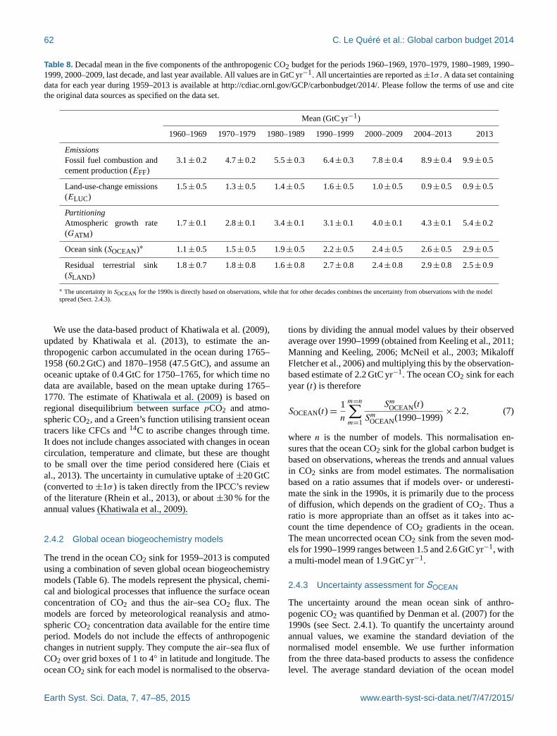
62 C. Le Quéré et al.: Global carbon budget 2014
Table 8. Decadal mean in the five components of the anthropogenic CO2 budget for the periods 1960–1969, 1970–1979, 1980–1989, 1990–
1999, 2000–2009, last decade, and last year available. All values are in GtC yr−1. All uncertainties are reported as±1σ . A data set containing
data for each year during 1959–2013 is available at http://cdiac.ornl.gov/GCP/carbonbudget/2014/. Please follow the terms of use and cite
the original data sources as specified on the data set.
Mean (GtC yr−1)
1960–1969 1970–1979 1980–1989 1990–1999 2000–2009 2004–2013 2013
Emissions
Fossil fuel combustion and
cement production (EFF)
3.1± 0.2 4.7± 0.2 5.5± 0.3 6.4± 0.3 7.8± 0.4 8.9± 0.4 9.9± 0.5
Land-use-change emissions
(ELUC)
1.5± 0.5 1.3± 0.5 1.4± 0.5 1.6± 0.5 1.0± 0.5 0.9± 0.5 0.9± 0.5
Partitioning
Atmospheric growth rate
(GATM)
1.7± 0.1 2.8± 0.1 3.4± 0.1 3.1± 0.1 4.0± 0.1 4.3± 0.1 5.4± 0.2
Ocean sink (SOCEAN)∗ 1.1± 0.5 1.5± 0.5 1.9± 0.5 2.2± 0.5 2.4± 0.5 2.6± 0.5 2.9± 0.5
Residual terrestrial sink
(SLAND)
1.8± 0.7 1.8± 0.8 1.6± 0.8 2.7± 0.8 2.4± 0.8 2.9± 0.8 2.5± 0.9
∗ The uncertainty in SOCEAN for the 1990s is directly based on observations, while that for other decades combines the uncertainty from observations with the model
spread (Sect. 2.4.3).
We use the data-based product of Khatiwala et al. (2009),
updated by Khatiwala et al. (2013), to estimate the an-
thropogenic carbon accumulated in the ocean during 1765–
1958 (60.2 GtC) and 1870–1958 (47.5 GtC), and assume an
oceanic uptake of 0.4 GtC for 1750–1765, for which time no
data are available, based on the mean uptake during 1765–
1770. The estimate of Khatiwala et al. (2009) is based on
regional disequilibrium between surface pCO2 and atmo-
spheric CO2, and a Green’s function utilising transient ocean
tracers like CFCs and 14C to ascribe changes through time.
It does not include changes associated with changes in ocean
circulation, temperature and climate, but these are thought
to be small over the time period considered here (Ciais et
al., 2013). The uncertainty in cumulative uptake of ±20 GtC
(converted to ±1σ ) is taken directly from the IPCC’s review
of the literature (Rhein et al., 2013), or about ±30 % for the
annual values (Khatiwala et al., 2009).
2.4.2 Global ocean biogeochemistry models
The trend in the ocean CO2 sink for 1959–2013 is computed
using a combination of seven global ocean biogeochemistry
models (Table 6). The models represent the physical, chemi-
cal and biological processes that influence the surface ocean
concentration of CO2 and thus the air–sea CO2 flux. The
models are forced by meteorological reanalysis and atmo-
spheric CO2 concentration data available for the entire time
period. Models do not include the effects of anthropogenic
changes in nutrient supply. They compute the air–sea flux of
CO2 over grid boxes of 1 to 4◦ in latitude and longitude. The
ocean CO2 sink for each model is normalised to the observa-
tions by dividing the annual model values by their observed
average over 1990–1999 (obtained from Keeling et al., 2011;
Manning and Keeling, 2006; McNeil et al., 2003; Mikaloff
Fletcher et al., 2006) and multiplying this by the observation-
based estimate of 2.2 GtC yr−1. The ocean CO2 sink for each
year (t) is therefore
SOCEAN(t)=1
n
m=n∑m=1
SmOCEAN(t)
SmOCEAN(1990–1999)× 2.2, (7)
where n is the number of models. This normalisation en-
sures that the ocean CO2 sink for the global carbon budget is
based on observations, whereas the trends and annual values
in CO2 sinks are from model estimates. The normalisation
based on a ratio assumes that if models over- or underesti-
mate the sink in the 1990s, it is primarily due to the process
of diffusion, which depends on the gradient of CO2. Thus a
ratio is more appropriate than an offset as it takes into ac-
count the time dependence of CO2 gradients in the ocean.
The mean uncorrected ocean CO2 sink from the seven mod-
els for 1990–1999 ranges between 1.5 and 2.6 GtC yr−1, with
a multi-model mean of 1.9 GtC yr−1.
2.4.3 Uncertainty assessment for SOCEAN
The uncertainty around the mean ocean sink of anthro-
pogenic CO2 was quantified by Denman et al. (2007) for the
1990s (see Sect. 2.4.1). To quantify the uncertainty around
annual values, we examine the standard deviation of the
normalised model ensemble. We use further information
from the three data-based products to assess the confidence
level. The average standard deviation of the ocean model
Earth Syst. Sci. Data, 7, 47–85, 2015 www.earth-syst-sci-data.net/7/47/2015/

C. Le Quéré et al.: Global carbon budget 2014 63
ensemble is 0.15 GtC yr−1 during 1980–2010 (with a maxi-
mum of 0.22), but it increases as the model ensemble goes
back in time, with a standard deviation of 0.28 GtC yr−1
across models in the 1960s. We estimate that the uncer-
tainty in the annual ocean CO2 sink is about ±0.5 GtC yr−1
from the fractional uncertainty in the data uncertainty of
±0.4 GtC yr−1 and standard deviation across models of up to
±0.28 GtC yr−1, reflecting both the uncertainty in the mean
sink from observations during the 1990s (Denman et al.,
2007; Sect. 2.4.1) and in the interannual variability as as-
sessed by models.
We examine the consistency between the variability of the
model-based and the data-based products to assess confi-
dence in SOCEAN. The interannual variability of the ocean
fluxes (quantified as the standard deviation) of the three
data-based estimates for 1990–2009 (when they overlap) is
±0.37 GtC yr−1 (Rödenbeck et al., 2014), ±0.25 GtC yr−1
(Landschützer et al., 2014), and ±0.14 GtC yr−1 (Park et al.,
2010), compared to ±0.18 GtC yr−1 for the model mean.
The standard deviation includes a component of trend and
decadal variability in addition to interannual variability, and
their relative influence differs across estimates. The phase is
generally consistent between estimates, with a higher ocean
CO2 sink during El Niño events. The annual data-based esti-
mates correlate with the ocean CO2 sink estimated here with
a correlation of r = 0.36 (0.0 to 0.49 for individual mod-
els), r = 0.73 (0.54 to 0.68), and r = 0.64 (0.12 to 0.71) for
the data-based estimates of Rödenbeck et al. (2014), Land-
schützer et al. (2014), and Park et al. (2010), respectively
(simple linear regression), but their mutual correlation ranges
between 0.24 and 0.31 only. The use of annual data for the
correlation may reduce the strength of the relationship be-
cause the dominant source of variability associated with El
Niño events is less than 1 year. We assess a medium confi-
dence level to the annual ocean CO2 sink and its uncertainty
because they are based on multiple lines of evidence, and
the results are consistent in that the interannual variability in
the model and data-based estimates are all generally small
compared to the variability in atmospheric CO2 growth rate.
Nevertheless the various results do not show agreement in
interannual variability on the global scale or for the relative
roles of the annual and decadal variability compared to the
trend.
2.5 Terrestrial CO2 sink
The difference between the fossil fuel (EFF) and LUC net
emissions (ELUC), the growth rate in atmospheric CO2 con-
centration (GATM), and the ocean CO2 sink (SOCEAN) is at-
tributable to the net sink of CO2 in terrestrial vegetation and
soils (SLAND), within the given uncertainties. Thus, this sink
can be estimated as the residual of the other terms in the mass
balance budget, as well as directly calculated using DGVMs;
alternatively, it can be estimated from inverse models that
close a spatio-temporally explicit form of the mass balance
in Eq. (1). The residual land sink (SLAND) is thought to be
in part because of the fertilising effect of rising atmospheric
CO2 on plant growth, N deposition, and effects of climate
change such as the lengthening of the growing season in
northern temperate and boreal areas. SLAND does not include
gross land sinks directly resulting from LUC (e.g. regrowth
of vegetation) as these are estimated to be part of the net land-
use flux (ELUC). System boundaries make it difficult to ex-
actly attribute CO2 fluxes on land between SLAND and ELUC
(Erb et al., 2013), and by design most of the uncertainties in
our method are allocated to SLAND for those processes that
are poorly known or represented in models.
2.5.1 Residual of the budget
For 1959–2013, the terrestrial carbon sink was estimated
from the residual of the other budget terms by rearranging
Eq. (1):
SLAND = EFF+ELUC− (GATM+ SOCEAN). (8)
The uncertainty in SLAND is estimated annually from the
root sum of squares of the uncertainty in the right-hand terms
assuming the errors are not correlated. The uncertainty av-
erages to ±0.8 GtC yr−1 over 1959–2013 (Table 7). SLAND
estimated from the residual of the budget includes, by defi-
nition, all the missing processes and potential biases in the
other components of Eq. (8).
2.5.2 DGVMs
A comparison of the residual calculation of SLAND in Eq. (8)
with estimates from DGVMs as used to estimate ELUC in
Sect. 2.2.3, but here excluding the effects of changes in land
cover (using a constant pre-industrial land-cover distribu-
tion), provides an independent estimate of the consistency of
SLAND with our understanding of the functioning of the ter-
restrial vegetation in response to CO2 and climate variability
(Table 7). As described in Sect. 2.2.3, the DGVM runs that
exclude the effects of changes in land cover include all cli-
mate variability and CO2 effects over land but do not include
reductions in CO2 sink capacity associated with human ac-
tivity directly affecting changes in vegetation cover and man-
agement, which by design is allocated to ELUC. This effect
has been estimated to have led to a reduction in the terres-
trial sink by 0.5 GtC yr−1 since 1750 (Gitz and Ciais, 2003).
The models in this configuration estimate the mean and vari-
ability of SLAND based on atmospheric CO2 and climate, and
thus both terms can be compared to the budget residual.
The multi-DGVM mean of 2.5± 1.0 GtC yr−1 for the pe-
riod 2004–2013 agrees well with the value computed from
the budget residual (Table 7). The standard deviation of
the annual CO2 sink across the nine DGVMs ranges from
±0.4 to ±1.4 GtC yr−1, with a mean standard deviation of
±0.9 GtC yr−1 for the period 1959 to 2013. The model mean,
www.earth-syst-sci-data.net/7/47/2015/ Earth Syst. Sci. Data, 7, 47–85, 2015

64 C. Le Quéré et al.: Global carbon budget 2014
over different decades, correlates with the budget resid-
ual with r = 0.71, compared to correlations of r = 0.46 to
r = 0.70 (median of 0.61) between individual models. The
standard deviation is similar to that of the five model ensem-
bles presented in Le Quéré et al. (2009), but the correlation is
improved compared to r = 0.54 obtained in the earlier study.
The DGVM results suggest that the sum of our knowledge
on annual CO2 emissions and their partitioning is plausible
(see Discussion), and provide insight into the underlying pro-
cesses and regional breakdown. However as the standard de-
viation across the DGVMs (of±0.9 GtC yr−1) is of the same
magnitude as the combined uncertainty due to the other com-
ponents (EFF, ELUC, GATM, SOCEAN; Table 7), the DGVMs
do not provide further reduction of uncertainty on the terres-
trial CO2 sink compared to the residual of the budget (Eq. 8).
Yet, DGVM results are largely independent of the residual of
the budget, and it is worth noting that the residual method and
ensemble mean DGVM results are consistent within their re-
spective uncertainties. We assess a medium confidence level
to the annual land CO2 sink and its uncertainty because the
estimates from the residual budget and averaged DGVMs
match well within their respective uncertainties, and the es-
timates based on the residual budget are primarily dependent
on EFF and GATM, both of which are well constrained.
2.6 The atmospheric perspective
The worldwide network of atmospheric measurements can
be used with atmospheric inversion methods to constrain the
location of the combined total surface CO2 fluxes from all
sources, including fossil and LUC emissions and land and
ocean CO2 fluxes. As the geographical distribution of fossil
fuel emissions is already known, it can be subtracted from the
total surface CO2 flux to provide CO2 fluxes over land and
over the ocean. Here we used preliminary atmospheric CO2
data to the end of 2013, and three atmospheric CO2 inver-
sions (Table 6) to infer the total CO2 flux over land regions,
and the distribution of the total land and ocean CO2 fluxes for
the mid- to high-latitude Northern Hemisphere (30–90◦ N),
tropics (30◦ S–30◦ N) and mid- to high-latitude region of
the Southern Hemisphere (30–90◦ S). We focus here on the
largest and most consistent sources of information, and use
these estimates to comment on the consistency across various
data streams and process-based estimates.
Atmospheric inversions
The three inversion systems used in this release (Chevallier
et al., 2005; Peters et al., 2010; Rödenbeck, 2005) are based
on the same Bayesian inversion principles that interpret the
same, for the most part, observed time series (or subsets
thereof), but they use different methodologies that represent
some of the many approaches used in the field. This mainly
concerns the time resolution of the estimates (i.e. weekly or
monthly), spatial breakdown (i.e. grid size), assumed cor-
relation structures, and mathematical approach. The details
of these approaches are documented extensively in the ref-
erences provided. Each system had used a different trans-
port model, which was demonstrated to be a driving factor
behind differences in atmospheric-based flux estimates, and
specifically their global distribution (Stephens et al., 2007).
Most inverse models use estimates for the ocean and land
biosphere, which can be very similar to those described in
Sects. 2.4.1 and 2.5.1 to assign prior fluxes. They do not
estimate EFF separately but assign EFF using similar data
sources to those used described in Sects. 2.1.1 and 2.2.2. Fi-
nally atmospheric inversions include CO2 fluxes from rivers
(which need to be taken into account to allow comparison
to other sources) and chemical oxidation of reactive carbon-
containing gases (which are neglected here). These inverse
estimates are not truly independent of the other estimates pre-
sented here as the atmospheric observations include a set of
observations used to estimate the global atmospheric growth
rate (Sect. 2.3). However they provide new information on
the regional distribution of fluxes.
In this first application of inverse methods to the car-
bon budget we focus the analysis on two known strengths
of the inverse approach: the derivation of the year-to-
year changes in total land (ELUC+ SLAND) fluxes con-
sistent with the whole network of atmospheric obser-
vations, and the spatial breakdown of land and ocean
fluxes (ELUC+ SLAND+ SOCEAN) across large regions of the
global. The total land flux correlates well with those esti-
mated from the budget residual (Eq. 1) with corrections for
the annual time series ranging from r = 0.84 to 0.93, and
with the DGVM multi-model mean with correlations for the
annual time series ranging from r = 0.71 to 0.84 (r = 0.37
to 0.82 for individual DGVMs and inversions). The spatial
breakdown is discussed in Sect. 3.1.3.
2.7 Processes not included in the global carbon budget
2.7.1 Contribution of anthropogenic CO and CH4 to the
global carbon budget
Anthropogenic emissions of CO and CH4 to the atmosphere
are eventually oxidised to CO2 and are thus part of the global
carbon budget. These contributions are omitted in Eq. (1), but
an attempt is made in this section to estimate their magnitude
and identify the sources of uncertainty. Anthropogenic CO
emissions are from incomplete fossil fuel and biofuel burning
and deforestation fires. The main anthropogenic emissions
of fossil CH4 that matter for the global carbon budget are
the fugitive emissions of coal, oil, and gas upstream sectors
(see below). These emissions of CO and CH4 contribute a net
addition of fossil carbon to the atmosphere.
In our estimate of EFF we assumed (Sect. 2.1.1) that all
the fuel burned is emitted as CO2; thus CO anthropogenic
emissions and their atmospheric oxidation into CO2 within a
few months are already counted implicitly in EFF and should
Earth Syst. Sci. Data, 7, 47–85, 2015 www.earth-syst-sci-data.net/7/47/2015/

C. Le Quéré et al.: Global carbon budget 2014 65
not be counted twice (same for ELUC and anthropogenic CO
emissions by deforestation fires). Anthropogenic emissions
of fossil CH4 are not included in EFF, because these fugi-
tive emissions are not included in the fuel inventories. Yet
they contribute to the annual CO2 growth rate after CH4
gets oxidised into CO2. Anthropogenic emissions of fossil
CH4 represent 15 % of total CH4 emissions (Kirschke et al.,
2013), which is 0.061 GtC yr−1 for the past decade. Assum-
ing steady state, these emissions are all converted to CO2 by
OH oxidation, thus explaining 0.06 GtC yr−1 of the global
CO2 growth rate in the past decade.
Other anthropogenic changes in the sources of CO and
CH4 from wildfires, biomass, wetlands, ruminants, or per-
mafrost changes are similarly assumed to have a small effect
on the CO2 growth rate.
2.7.2 Anthropogenic carbon fluxes in the
land-to-ocean continuum
The approach used to determine the global carbon budget
considers only anthropogenic CO2 emissions and their parti-
tioning among the atmosphere, ocean, and land. In this anal-
ysis, the land and ocean reservoirs that take up anthropogenic
CO2 from the atmosphere are conceived as independent car-
bon storage repositories. This approach thus omits that car-
bon is continuously displaced along the land–ocean aquatic
continuum (LOAC) comprising freshwaters, estuaries, and
coastal areas (Bauer et al., 2013; Regnier et al., 2013). A sig-
nificant fraction of this lateral carbon flux is entirely “natu-
ral” and is thus a steady-state component of the pre-industrial
carbon cycle that can be ignored in the current analysis. The
remaining fraction is anthropogenic carbon entrained into the
lateral transport loop of the LOAC, a perturbation that is rel-
evant for the global carbon budget presented here.
The results of the analysis of Regnier et al. (2013) can be
summarised in three points of relevance to the anthropogenic
CO2 budget. First, the anthropogenic carbon input from land
to hydrosphere, FLH, estimated at 1± 0.5 PgC is significant
compared to the other terms of Eq. (1) (Table 8), and im-
plies that only a portion of the anthropogenic CO2 taken up
by land ecosystems remains sequestered in soil and biomass
pools. Second, some of the exported anthropogenic carbon
is stored in the LOAC (1CLOAC, 0.55± 0.3 GtC yr−1) and
some is released back to the atmosphere as CO2 (ELOAC,
0.35± 0.2 GtC yr−1), the magnitude of these fluxes result-
ing from the combined effects of freshwaters, estuaries, and
coastal seas. Third, a small fraction of anthropogenic car-
bon displaced by the LOAC is transferred to the open ocean,
where it accumulates (FHO, 0.1±> 0.05 GtC yr−1). The an-
thropogenic perturbation of the carbon fluxes from land to
ocean does not contradict the method used in Sect. 2.5 to de-
fine the ocean sink and residual land sink. However, it does
point to the need to account for the fate of anthropogenic car-
bon once it is removed from the atmosphere by land ecosys-
tems (summarised in Fig. 2). In theory, direct estimates of
changes of the ocean inorganic carbon inventory over time
would see the land flux of anthropogenic carbon and would
thus have a bias relative to air–sea flux estimates and tracer-
based reconstructions. However, currently the value is small
enough to be not noticeable relative to the errors in the indi-
vidual techniques.
More importantly the residual land sink calculated in
a budget which accounts for the LOAC (SLAND+LOAC =
3.25± 0.9 GtC yr−1) is larger than the residual land sink
(SLAND) value of 2.9± 0.85 GtC yr−1 (2004–2013) calcu-
lated according to Eq. (8). This is because this flux is par-
tially offset by the net source of CO2 to the atmosphere of
0.35± 0.3 GtC yr−1 from rivers, estuaries, and coastal seas
(ELOAC):
SLAND+LOAC = EFF+ELUC− (GATM+ SOCEAN)
+ELOAC. (9)
In addition, because a fraction of anthropogenic CO2 taken
up by land ecosystems is exported to the LOAC (FLH),
the annual terrestrial ecosystems carbon storage change
comprising the land vegetation, litter, and soil (1CTE,
1.35 GtC yr−1) is notably smaller than what would be cal-
culated in a traditional budget that ignores the LOAC. In this
case, the carbon storage change for the period 2004–2013
(Table 8) is estimated to be 2 Gt C yr−1 from the difference
between SLAND (2.9 GtC yr−1) and ELUC (0.9 GtC yr−1).
With the LOAC included, we now have
1CTE = SLAND+LOAC−ELUC−FLH. (10)
A significant fraction of the anthropogenic carbon dis-
placed from land ecosystems to LOAC is stored in freshwater
and coastal sediments (1CLOAC) and, to a lesser extent, in
the open ocean (FHO), while the rest is re-emitted to the at-
mosphere by freshwaters (ELOAC). The annual ocean carbon
storage change with LOAC included (1COCEAN) is therefore
equal to 1COCEAN = SOCEAN+FHO.
All estimates of LOAC are given with low confidence, be-
cause they originate from a single source. The carbon bud-
get presented here implicitly incorporates the fluxes from
the LOAC with SLAND. We do not attempt to separate these
fluxes, because the uncertainties in either estimate are too
large and there is insufficient information available to esti-
mate the LOAC fluxes on an annual basis.
3 Results
3.1 Global carbon budget averaged over decades and
its variability
The global carbon budget averaged over the last decade
(2004–2013) is shown in Fig. 2. For this time period, 91 %
of the total emissions (EFF+ELUC) were caused by fossil
fuel combustion and cement production, and 9 % by land-
use change. The total emissions were partitioned among the
www.earth-syst-sci-data.net/7/47/2015/ Earth Syst. Sci. Data, 7, 47–85, 2015

66 C. Le Quéré et al.: Global carbon budget 2014
Time (yr)
CO
2 flux
(G
tC y
r−1 )
Emissions
Partitioning
Fossil fuels and cement
Land−use change
Land
Atmosphere
Ocean
1900 1950 2000
10
5
0
5
10
Figure 3. Combined components of the global carbon budget il-
lustrated in Fig. 2 as a function of time for emissions from fossil
fuel combustion and cement production (EFF; grey) and emissions
from land-use change (ELUC; brown), as well as their partitioning
among the atmosphere (GATM; light blue), land (SLAND; green),
and oceans (SOCEAN; dark blue). All time series are in GtC yr−1.
GATM and SOCEAN (and by construction also SLAND) prior to
1959 are based on different methods. The primary data sources
for fossil fuel and cement emissions are from Boden et al. (2013),
with uncertainty of about ±5 % (±1σ ); land-use-change emis-
sions are from Houghton et al. (2012) with uncertainties of about
±30 %; the atmospheric growth rate prior to 1959 is from Joos and
Spahni (2008) with uncertainties of about ±1–1.5 GtC decade−1
or ±0.1–0.15 GtC yr−1 (Bruno and Joos, 1997), and from Dlu-
gokencky and Tans (2014) from 1959 with uncertainties of about
±0.2 GtC yr−1; the ocean sink prior to 1959 is from Khatiwala et
al. (2013) with uncertainty of about ±30 %, and from this study
from 1959 with uncertainties of about±0.5 GtC yr−1; and the resid-
ual land sink is obtained by difference (Eq. 8), resulting in uncer-
tainties of about ±50 % prior to 1959 and ±0.8 GtC yr−1 after that.
See the text for more details of each component and their uncertain-
ties.
atmosphere (44 %), ocean (26 %), and land (29 %). All com-
ponents except land-use-change emissions have grown since
1959 (Figs. 3 and 4), with important interannual variability in
the atmospheric growth rate and in the land CO2 sink (Fig. 4),
as well as some decadal variability in all terms (Table 8).
3.1.1 CO2 emissions
Global CO2 emissions from fossil fuel combustion and ce-
ment production have increased every decade from an av-
erage of 3.1± 0.2 GtC yr−1 in the 1960s to an average of
8.9± 0.4 GtC yr−1 during 2004–2013 (Table 8 and Fig. 5).
1960 1970 1980 1990 2000 20100
2
4
6
8
10
12Fossil fuels and cementa
1960 1970 1980 1990 2000 2010
0
2
4
6
8
10
Time (yr)
CO
2 em
issi
ons
(GtC
yr−
1 )
b Land−use change
1960 1970 1980 1990 2000 2010
0
2
4
6
8
10 Atmospheric growthc
1960 1970 1980 1990 2000 2010
0
2
4
6
8
10 Ocean sinkd
CO
2 par
titio
ning
(G
tC y
r−1 )
1960 1970 1980 1990 2000 2010−2
0
2
4
6
8
10Land sinke
Time (yr)
Figure 4. Components of the global carbon budget and their uncer-
tainties as a function of time, presented individually for (a) emis-
sions from fossil fuel combustion and cement production (EFF),
(b) emissions from land-use change (ELUC), (c) atmospheric CO2
growth rate (GATM), (d) the ocean CO2 sink (SOCEAN; positive in-
dicates a flux from the atmosphere to the ocean), and (e) the land
CO2 sink (SLAND; positive indicates a flux from the atmosphere
to the land). All time series are in GtC yr−1, with the uncertainty
bounds representing ±1σ in shaded colour. Data sources are as in
Fig. 2. The black dots in panels (a), (b), and (e) show values for
2011, 2012, and 2013 that originate from a different data set to the
remainder of the data, as explained in the text.
The growth rate in these emissions decreased between the
1960s and the 1990s, from 4.5 % yr−1 in the 1960s (1960–
1969), to 2.9 % yr−1 in the 1970s (1970–1979), to 1.9 % yr−1
in the 1980s (1980–1989), and finally to 1.0 % yr−1 in the
1990s (1990–1999), before it began increasing again in the
2000s at an average growth rate of 3.3 % yr−1, decreasing
slightly thereafter to 2.5 % yr−1 for the last decade (2004–
2013). In contrast, CO2 emissions from LUC have remained
constant, in our analysis at around 1.5± 0.5 GtC yr−1 be-
tween 1960 and 1999 and 0.9± 0.5 GtC yr−1 during 2004–
2013. TheELUC estimates from the bookkeeping method and
the DGVM models are consistent within their respective un-
certainties (Table 7 and Fig. 6). However, whereas the de-
crease in emissions from LUC between the 1990s and 2000s
is also present in the DGVMs (Fig. 6), it was not found in the
study of tropical deforestation of Achard et al. (2014), where
the fluxes in the 1990s were similar to those of the 2000s and
outside our uncertainty range.
Earth Syst. Sci. Data, 7, 47–85, 2015 www.earth-syst-sci-data.net/7/47/2015/

C. Le Quéré et al.: Global carbon budget 2014 67
1960 1970 1980 1990 2000 20100
2
4
6
8
10
12
Global
a
1960 1970 1980 1990 2000 20100
1
2
3
4
5
Coal
Oil
Gas
Cement
b
CO
2 em
issi
ons
(GtC
yr−
1 )
1960 1970 1980 1990 2000 20100
1
2
3
4
5
6
Time (yr)
Annex B
Non−Annex B
Emissions transfers
c
1960 1970 1980 1990 2000 20100
0.5
1
1.5
2
2.5
3
China
USA
EU28
India
d
CO
2 em
issi
ons
(GtC
yr−
1 )
1960 1970 1980 1990 2000 20100
1
2
3
4
5
6
7
Time (yr)
India
USA
China
EU28
Global
e
Per
cap
ita e
mis
sion
s (t
C p
erso
n−1 y
r−1 )
Figure 5. CO2 emissions from fossil fuel combustion and cement
production for (a) the globe, including an uncertainty of ±5 %
(grey shading), the emissions extrapolated using BP energy statis-
tics (black dots) and the emissions projection for year 2014 based
on GDP projection (red dot); (b) global emissions by fuel type, in-
cluding coal (red), oil (black), gas (blue), and cement (purple) and
excluding gas flaring, which is small (0.6 % in 2013); (c) territorial
(full line) and consumption (dashed line) emissions for the coun-
tries listed in Annex B of the Kyoto Protocol (blue lines; mostly
advanced economies with emissions limitations) versus non-Annex
B countries (red lines) – also shown are the emission transfers from
non-Annex B to Annex B countries (black line); (d) territorial CO2
emissions for the top three country emitters (USA – purple; China
– red; India – green) and for the European Union (EU; blue for
the 28 member states of the EU in 2012); and (e) per capita emis-
sions for the top three country emitters and the EU (all colours as in
panel d) and the world (black). In (b) to (e), the dots show the data
that were extrapolated from BP energy statistics for 2011, 2012, and
2013. All time series are in GtC yr−1 except the per capita emis-
sions (panel e), which are in tonnes of carbon per person per year
(tC person−1 yr−1). All territorial emissions are primarily from Bo-
den et al. (2013) as detailed in the text; consumption-based emis-
sions are updated from Peters et al. (2011a).
3.1.2 Partitioning
The growth rate in atmospheric CO2 increased from
1.7± 0.1 GtC yr−1 in the 1960s to 4.3± 0.1 GtC yr−1 dur-
ing 2004–2013 with important decadal variations (Table 8).
Both ocean and land CO2 sinks increased roughly in line
with the atmospheric increase, but with significant decadal
variability on land (Table 8). The ocean CO2 sink increased
from 1.1± 0.5 GtC yr−1 in the 1960s to 2.6± 0.5 GtC yr−1
1960 1970 1980 1990 2000 2010−4
−2
0
2
4
6
CO
2 (G
tC y
r−1 )
a
Land−use change
1960 1970 1980 1990 2000 2010−4
−2
0
2
4
6
CO
2 (G
tC y
r−1 )
b
Land sink
1960 1970 1980 1990 2000 2010−4
−2
0
2
4
6
Time (yr)
CO
2 (G
tC y
r−1 )
c
Total land
Figure 6. Comparison of the atmosphere–land CO2 flux showing
budget values of ELUC (black line). (a) CO2 emissions from land-
use change showing individual DGVM model results (green) and
the multi-model mean (yellow line), and fire-based results (brown);
LUC data prior to 1997 (dashed black line) highlights the start of
satellite data from that year. (b) Land CO2 sink (SLAND) show-
ing individual DGVM model results (green) and multi-model mean
(yellow line). (c) Total land CO2 fluxes (sum of a+b) from DGVM
model results (green) and the multi-model mean (yellow line), at-
mospheric inversions (MACC, v13.1 (Chevallier et al., 2005) in red;
Rödenbeck et al. (2003) in orange; Peters et al. (2010) in purple;
see Table 6), and the carbon balance from Eq. (1) (black). In (c) the
inversions were corrected for the pre-industrial land sink of CO2
from river input by adding a sink of 0.45 GtC yr−1 (Jacobson et al.,
2007). This correction does not take into account the anthropogenic
contribution to river fluxes (see Sect. 2.7.2).
during 2004–2013, with interannual variations of the order
of a few tenths of GtC yr−1 generally showing an increased
ocean sink during El Niño events (i.e. 1982–1983, 1991–
1993, 1997–1998) (Fig. 7; Rödenbeck et al., 2014). Although
there is some coherence between the ocean models and data
www.earth-syst-sci-data.net/7/47/2015/ Earth Syst. Sci. Data, 7, 47–85, 2015

68 C. Le Quéré et al.: Global carbon budget 2014
products and among data products, their mutual correlation
is weak and highlights disagreement on the exact amplitude
of the interannual variability, as well as on the relative im-
portance of the trend versus the variability (Sect. 2.4.3 and
Fig. 7). Most estimates produce a mean CO2 sink for the
1990s that is below the mean assessed by the IPCC from in-
direct (but arguably more reliable) observations (Denman et
al., 2007; Sect. 2.4.1). This could reflect issues with the verti-
cal diffusion in ocean models, although as the data products
also support a lower mean CO2 sink, this discrepancy sug-
gests we may need to reassess estimates of the mean ocean
carbon sinks.
The land CO2 sink increased from 1.8± 0.7 GtC yr−1 in
the 1960s to 2.9± 0.8 GtC yr−1 during 2004–2013, with im-
portant interannual variations of up to 2 GtC yr−1 gener-
ally showing a decreased land sink during El Niño events,
overcompensating for the increased in ocean sink and ac-
counting for the enhanced atmospheric growth rate dur-
ing El Niño events (Poulter et al., 2014). The high-uptake
anomaly around year 1991 is thought to be caused by the
effect of the volcanic eruption of Mount Pinatubo on cli-
mate (Achard et al., 2014; Fig. 6c) and is not generally re-
produced by the DGVMs but assigned to SLAND by the two
inverse systems that include this period (Fig. 6). The larger
land CO2 sink during 2004–2013 compared to the 1960s is
reproduced by all the DGVMs in response to combined at-
mospheric CO2 increase, climate, and variability (average
change of 1.4 GtC yr−1; eight models ranging between 0.8
and 2.3 GtC yr−1 with one model at 0.1 GtC yr−1), consistent
with the budget residual and reflecting a common knowledge
of the processes (Table 7). The decadal change is also consis-
tent with the results from the atmospheric inversions, which
estimate a trend of 0.84 and 0.62 GtC yr−1 per decade for
the inversions of Chevallier et al. (2005) and Rödenbeck et
al. (2003), respectively.
The total CO2 fluxes on land (ELUC+ SLAND) constrained
by the atmospheric inversions show in general very good
agreement with the global budget estimate, as expected given
the strong constrains of GATM and the small relative uncer-
tainty typically assumed on SOCEAN and EFF by inversions.
The total sink of similar magnitude for the decadal aver-
age, with estimates for 2004–2013 from the inversions of
1.7, 2.0, and 3.1 GtC yr−1 compared to 2.0±−0.7 GtC yr−1
for the budget residual (Table 7). The inversions’ total land
sink would be 1.2, 1.5, and 2.6 GtC yr−1 when including a
mean river flux correction of 0.45 GtC yr−1, though the ex-
act correction would be smaller when taking into account
the anthropogenic contribution to river fluxes (Sect. 2.7.2).
The interannual variability of the inversions also matched
the residual-based SLAND closely (Fig. 6). The multi-model
mean from the DGVM ensemble that preformed the LUC
simulations also compares well with the estimate from the
residual budget and atmospheric inversions, with a decadal
mean of 1.4±−1.0 GtC yr−1 (Table 7; 2004–2013), al-
1960 1970 1980 1990 2000 20100
1
2
3
4
Time (yr)
CO
2 (G
tC y
r−1 )
Figure 7. Comparison of the atmosphere–ocean CO2 flux shows
the budget values of SOCEAN (black line), individual ocean mod-
els before normalisation (blue lines), and the three ocean data-
based products (Rödenbeck et al. (2014) in orange, Landschützer
et al. (2014) in red, and Park et al. (2010) in purple; see Table 6).
All data-based products were corrected for the pre-industrial ocean
source of CO2 from river input to the ocean, which is not present
in the models, by adding a sink of 0.45 GtC yr−1 (Jacobson et al.,
2007) in order to make them comparable to SOCEAN. This correc-
tion does not take into account the anthropogenic contribution to
river fluxes (see Sect. 2.7.2).
though individual models differ by several gigatonnes of car-
bon for some years (Fig. 6).
3.1.3 Distribution
The total surface CO2 fluxes on land and ocean includ-
ing LUC (ELUC+ SLAND+ SOCEAN) estimated from process
models and atmospheric inversions can provide information
on the regional distribution of those fluxes by latitude band
(Fig. 8). The global mean CO2 fluxes from process models
for 2004–2013 is 2.8 GtC yr−1, an underestimate compared
to the fluxes of 4.5 GtC yr−1 inferred from the remainder of
the carbon budget (EFF−GATM in Eq. 1; Table 8). In con-
trast, the total CO2 fluxes from the three inversions range be-
tween 4.1 and 4.7 GtC yr−1, consistent with the carbon bud-
get as expected from the constraints on the inversions.
In the south (south of 30◦ S), the atmospheric inversions
and combined models all suggest a CO2 sink for 2004–2013
of between 1.3 and 1.6 GtC yr−1 (Fig. 8), although the de-
tails of the interannual variability are not fully consistent
across methods. The interannual variability in the south is
low because of the dominance of ocean area with low vari-
ability compared to land areas. In the tropics (30◦ S–30◦ N),
both the atmospheric inversions and combined models sug-
gest the carbon balance in this region is close to neutral over
the past decade, with fluxes for 2004–2013 ranging between
−0.3 and +0.4 GtC yr−1. This region also shows the largest
variability, both on interannual and decadal timescales.
In the north (north of 30◦ N), the inversions and com-
bined models disagree on the magnitude of the CO2 sink,
Earth Syst. Sci. Data, 7, 47–85, 2015 www.earth-syst-sci-data.net/7/47/2015/
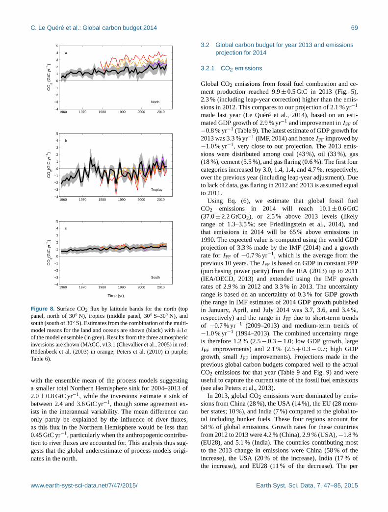
C. Le Quéré et al.: Global carbon budget 2014 69
1960 1970 1980 1990 2000 2010−4
−3
−2
−1
0
1
2
3
4
5C
O2 (
GtC
yr−
1 )a
North
1960 1970 1980 1990 2000 2010−4
−3
−2
−1
0
1
2
3
4
5
CO
2(GtC
yr−
1 )
b
Tropics
1960 1970 1980 1990 2000 2010−4
−3
−2
−1
0
1
2
3
4
5
Time (yr)
CO
2(GtC
yr−
1 )
c
South
Figure 8. Surface CO2 flux by latitude bands for the north (top
panel, north of 30◦ N), tropics (middle panel, 30◦ S–30◦ N), and
south (south of 30◦ S). Estimates from the combination of the multi-
model means for the land and oceans are shown (black) with ±1σ
of the model ensemble (in grey). Results from the three atmospheric
inversions are shown (MACC, v13.1 (Chevallier et al., 2005) in red;
Rödenbeck et al. (2003) in orange; Peters et al. (2010) in purple;
Table 6).
with the ensemble mean of the process models suggesting
a smaller total Northern Hemisphere sink for 2004–2013 of
2.0± 0.8 GtC yr−1, while the inversions estimate a sink of
between 2.4 and 3.6 GtC yr−1, though some agreement ex-
ists in the interannual variability. The mean difference can
only partly be explained by the influence of river fluxes,
as this flux in the Northern Hemisphere would be less than
0.45 GtC yr−1, particularly when the anthropogenic contribu-
tion to river fluxes are accounted for. This analysis thus sug-
gests that the global underestimate of process models origi-
nates in the north.
3.2 Global carbon budget for year 2013 and emissions
projection for 2014
3.2.1 CO2 emissions
Global CO2 emissions from fossil fuel combustion and ce-
ment production reached 9.9± 0.5 GtC in 2013 (Fig. 5),
2.3 % (including leap-year correction) higher than the emis-
sions in 2012. This compares to our projection of 2.1 % yr−1
made last year (Le Quéré et al., 2014), based on an esti-
mated GDP growth of 2.9 % yr−1 and improvement in IFF of
−0.8 % yr−1 (Table 9). The latest estimate of GDP growth for
2013 was 3.3 % yr−1 (IMF, 2014) and hence IFF improved by
−1.0 % yr−1, very close to our projection. The 2013 emis-
sions were distributed among coal (43 %), oil (33 %), gas
(18 %), cement (5.5 %), and gas flaring (0.6 %). The first four
categories increased by 3.0, 1.4, 1.4, and 4.7 %, respectively,
over the previous year (including leap-year adjustment). Due
to lack of data, gas flaring in 2012 and 2013 is assumed equal
to 2011.
Using Eq. (6), we estimate that global fossil fuel
CO2 emissions in 2014 will reach 10.1± 0.6 GtC
(37.0± 2.2 GtCO2), or 2.5 % above 2013 levels (likely
range of 1.3–3.5 %; see Friedlingstein et al., 2014), and
that emissions in 2014 will be 65 % above emissions in
1990. The expected value is computed using the world GDP
projection of 3.3 % made by the IMF (2014) and a growth
rate for IFF of −0.7 % yr−1, which is the average from the
previous 10 years. The IFF is based on GDP in constant PPP
(purchasing power parity) from the IEA (2013) up to 2011
(IEA/OECD, 2013) and extended using the IMF growth
rates of 2.9 % in 2012 and 3.3 % in 2013. The uncertainty
range is based on an uncertainty of 0.3 % for GDP growth
(the range in IMF estimates of 2014 GDP growth published
in January, April, and July 2014 was 3.7, 3.6, and 3.4 %,
respectively) and the range in IFF due to short-term trends
of −0.7 % yr−1 (2009–2013) and medium-term trends of
−1.0 % yr−1 (1994–2013). The combined uncertainty range
is therefore 1.2 % (2.5− 0.3− 1.0; low GDP growth, large
IFF improvements) and 2.1 % (2.5+ 0.3− 0.7; high GDP
growth, small IFF improvements). Projections made in the
previous global carbon budgets compared well to the actual
CO2 emissions for that year (Table 9 and Fig. 9) and were
useful to capture the current state of the fossil fuel emissions
(see also Peters et al., 2013).
In 2013, global CO2 emissions were dominated by emis-
sions from China (28 %), the USA (14 %), the EU (28 mem-
ber states; 10 %), and India (7 %) compared to the global to-
tal including bunker fuels. These four regions account for
58 % of global emissions. Growth rates for these countries
from 2012 to 2013 were 4.2 % (China), 2.9 % (USA),−1.8 %
(EU28), and 5.1 % (India). The countries contributing most
to the 2013 change in emissions were China (58 % of the
increase), the USA (20 % of the increase), India (17 % of
the increase), and EU28 (11 % of the decrease). The per
www.earth-syst-sci-data.net/7/47/2015/ Earth Syst. Sci. Data, 7, 47–85, 2015

70 C. Le Quéré et al.: Global carbon budget 2014
Table 9. Actual CO2 emissions from fossil fuel combustion and cement production (EFF) compared to projections made the previous year
based on world GDP (IMF October 2013) and the fossil fuel intensity of GDP (IFF) based on subtracting the CO2 and GDP growth rates.
The “Actual” values are the latest estimate available, and the “Projected” value for 2013 refers to those estimates presented in this paper. A
correction for leap years is applied (Sect. 2.1.3).
2009a 2010b 2011c 2012d 2013e 2014f
Pro
ject
ed
Act
ual
Pro
ject
ed
Act
ual
Pro
ject
ed
Act
ual
Pro
ject
ed
Act
ual
Pro
ject
ed
Act
ual
Pro
ject
ed
EFF −2.8 % −0.5 % > 3 % 4.9 % 3.1± 1.5 % 3.2 % 2.6 % 2.2 % 2.1 2.3 % 2.5 %
(1.9–3.5) (1.1–3.1) (1.3–3.5)
GDP −1.1 % −0.4 % 4.8 % 5.2 % 4.0 % 3.9 % 3.3 % 3.2 % 2.9 % 3.2 % 3.3 %
IFF −1.7 % −0.9 % >−1.7 % −0.3 % −0.9± 1.5 % −0.7 % −0.7 % −1.0 % −0.8 % −0.9 % −0.7 %
a Le Quéré et al. (2009). b Friedlingstein et al. (2010). c Peters et al. (2013). d Le Quéré et al. (2013). e Le Quéré et al. (2014). f Friedlingstein et al. (2014) and this study.
1960 1970 1980 1990 2000 20100
2
4
6
8
10
12Fossil fuels and cementa
200620072008
200920102011
201220132014
1960 1970 1980 1990 2000 20100
1
2
3
4b Land−use change
Time (yr)
CO
2 em
issi
ons
(GtC
yr−
1 )
1960 1970 1980 1990 2000 20100
2
4
6
8c Atmospheric growth
1960 1970 1980 1990 2000 20100
1
2
3
4d Ocean sink
CO
2 par
titio
ning
(G
tC y
r−1 )
1960 1970 1980 1990 2000 2010−2
0
2
4
6e Land sink
Time (yr)
Figure 9. Comparison of global carbon budget components re-
leased annually by GCP since 2006. CO2 emissions from both
(a) fossil fuel combustion and cement production (EFF), and
(b) land-use change (ELUC), and their partitioning among (c) the
atmosphere (GATM), (d) ocean (SOCEAN), and (e) land (SLAND).
See legend for the corresponding years, with the 2006 carbon bud-
get from Raupach et al. (2007), 2007 from Canadell et al. (2007),
2008 released online only, 2009 from Le Quéré et al. (2009), 2010
from Friedlingstein et al. (2010), 2011 from Peters et al. (2012b),
2012 from Le Quéré et al. (2013), and 2013 from Le Quéré et
al. (2014) and this year’s budget (2014). The budget year gener-
ally corresponds to the year when the budget was first released. All
values are in GtC yr−1.
capita CO2 emissions in 2013 were 1.4 tC person−1 yr−1 for
the globe, and were 4.5 (USA), 2.0 (China), 1.9 (EU28)
and 0.5 tC person−1 yr−1 (India) for the four highest emitting
countries (Fig. 5e).
Territorial emissions in Annex B countries have remained
stable from 1990 to 2012, while consumption emissions grew
at 0.5 % yr−1 (Fig. 5c). In non-Annex B countries, territo-
rial emissions have grown at 4.4 % yr−1, while consump-
tion emissions have grown at 4.1 % yr−1. In 1990, 62 % of
global territorial emissions were emitted in Annex B coun-
tries (34 % in non-Annex B, and 4 % in bunker fuels used for
international shipping and aviation), while in 2012 this had
reduced to 37 % (58 % in non-Annex B, and 6 % in bunker
fuels). In terms of consumption emissions this split was 63 %
in 1990 and 43 % in 2012 (33 to 51 % in non-Annex B).
The difference between territorial and consumption emis-
sions (the net emission transfer via international trade) from
non-Annex B to Annex B countries has increased from
0.05 GtC yr−1 in 1990 to 0.46 GtC yr−1 in 2012 (Fig. 5), with
an average annual growth rate of 11 % yr−1. The increase in
net emission transfers of 0.41 GtC yr−1 from 1990 to 2012
compares with the emission reduction of 0.27 GtC yr−1 in
Annex B countries. These results clearly show a growing net
emission transfer via international trade from non-Annex B
to Annex B countries. In 2012, the biggest emitters from a
consumption perspective were China (23 % of the global to-
tal), the USA (16 %), EU28 (13 %), and India (6 %).
Based on DGVMs only, the global CO2 emissions from
land-use-change activities are estimated to be 0.9± 0.6 GtC
in 2013, slightly below the 2004–2013 average of
1.0± 0.7 GtC yr−1. However, although the decadal mean
generally agreed, the estimated annual variability was not
consistent between the LUC emissions estimated based on
the combined bookkeeping method and fire-based estimate
and the DGVMs, except that they are small relative to the
variability from the residual land sink (Fig. 6a). This could
be partly due to the design of the DGVM experiments, which
use flux differences between simulations with and without
Earth Syst. Sci. Data, 7, 47–85, 2015 www.earth-syst-sci-data.net/7/47/2015/

C. Le Quéré et al.: Global carbon budget 2014 71
land-cover change, and thus may overestimate variability due
to, for example, fires in forest regions where the contempo-
rary forest cover is smaller than pre-industrial cover used in
the runs without land-cover change. The extrapolated land-
cover input data for 2010–2013 may also explain part of the
discrepancy, though it would not account for the larger vari-
ability in the DGVMs.
3.2.2 Partitioning
The atmospheric CO2 growth rate was 5.4± 0.2 GtC in
2013 (2.53± 0.09 ppm, Fig. 4; Dlugokencky and Tans,
2014). This is significantly above the 2004–2013 average of
4.3± 0.1 GtC yr−1, though the interannual variability in at-
mospheric growth rate is large.
The ocean CO2 sink was 2.9± 0.5 GtC yr−1 in 2013, an
increase of 0.1 GtC yr−1 over 2012 according to ocean mod-
els. Five of the seven ocean models produce an increase in the
ocean CO2 sink in 2013 compared to 2012. However the two
data products available over that period produce a decrease of
−0.1 GtC yr−1. All estimates suggest relatively small change
in the ocean CO2 sink, consistent with El Niño neutral condi-
tions observed in 2013. All estimates suggest an ocean CO2
sink for 2013 that is larger than the 2004–2013 average of
2.6± 0.5 GtC yr−1. The terrestrial CO2 sink calculated as the
residual from the carbon budget was 2.5± 0.9 GtC in 2013,
just below the 2.7± 0.9 GtC in 2012 and the 2004–2013 av-
erage of 2.9± 0.8 GtC yr−1 (Fig. 4), and also consistent with
El Niño neutral conditions. The DGVM model mean sug-
gests the same terrestrial CO2 sink in 2013 of 2.4± 1.2 GtC
(Table 7), but results cover a range among models.
Cumulative emissions for 1870–2013 were 390± 20 GtC
for EFF and 145± 50 GtC for ELUC based on the bookkeep-
ing method of Houghton et al. (2012) for 1870–1996 and a
combination with fire-based emissions for 1997–2013 as de-
scribed in Sect. 2.2 (Table 10). The cumulative emissions are
rounded to the nearest 5 GtC. The total cumulative emissions
for 1870–2013 are 535± 55 GtC. These emissions were par-
titioned among the atmosphere (225± 5 GtC based on atmo-
spheric measurements in ice cores of 288 ppm (Sect. “Global
atmospheric CO2 growth rate estimates”; Joos and Spahni,
2008) and recent direct measurements of 395.31 ppm (Dlu-
gokencky and Tans, 2014)), ocean (150± 20 GtC using
Khatiwala et al., 2013, prior to 1959 and Table 8 otherwise),
and land (155± 60 GtC by the difference).
Cumulative emissions for the early period 1750–1869
were 3 GtC for EFF and about 45 GtC for ELUC (rounded
to nearest 5), of which 10 GtC was emitted in the period
1850–1870 (Houghton et al., 2012) and 30 GtC was emit-
ted in the period 1750–1850 based on the average of four
publications (22 GtC by Pongratz et al., 2009; 15 GtC by van
Minnen et al., 2009; 64 GtC by Shevliakova et al., 2009; and
24 GtC by Zaehle et al., 2011). The growth in atmospheric
CO2 during that time was about 25 GtC, and the ocean up-
take about 20 GtC, implying a land uptake of 5 GtC. These
numbers have large relative uncertainties but balance within
the limits of our understanding.
Cumulative emissions for 1750–2013 based on the sum
of the two periods above were 395± 20 GtC for EFF,
and 185± 65 GtC for ELUC, for a total of 580± 70 GtC,
partitioned among the atmosphere (250± 5 GtC), ocean
(170± 20 GtC), and land (160 ± 70 GtC).
Cumulative emissions through to year 2014 can be es-
timated based on the 2014 projections of EFF (Sect. 3.2),
the largest contributor, and assuming a constant ELUC
of 0.9 GtC. For 1870–2014, these are 545± 55 GtC
(2000± 200 GtCO2) for total emissions, with about 75 %
contribution from EFF (400± 20 GtC) and about 25 % con-
tribution from ELUC (145± 50 GtC). Cumulative emissions
since year 1870 are higher than the emissions of 515 [445
to 585] GtC reported in the IPCC (Stocker et al., 2013b) be-
cause they include an additional 32 GtC from emissions in
2012–2014 (mostly from EFF). The uncertainty presented
here (±1σ ) is smaller than the range of 90 % used by the
IPCC, but both estimates overlap within their uncertainty
ranges.
4 Discussion
Each year when the global carbon budget is published, each
component for all previous years is updated to take into ac-
count corrections that are due to further scrutiny and verifica-
tion of the underlying data in the primary input data sets. The
updates have generally been relatively small and focused on
the most recent years, except for LUC, where they are more
significant but still generally within the provided uncertainty
range (Fig. 9). The difficulty in accessing land-cover-change
data to estimate ELUC is the key problem to providing con-
tinuous records of emissions in this sector. Current FAO es-
timates are based on statistics reported at the country level
and are not spatially explicit. Advances in satellite recov-
ery of land-cover change could help to keep track of LUC
through time (Achard et al., 2014; Harris et al., 2014). Re-
visions in ELUC for the 2008/2009 budget were the result of
the release of FAO 2010, which contained a major update to
forest-cover change for the period 2000–2005 and provided
the data for the following 5 years to 2010 (Fig. 9b). The dif-
ferences in this year could be attributable to both the different
data and the different methods. Updates to values for any give
year in each component of the global carbon budget were
highest at 0.34 GtC yr−1 for the atmospheric growth rate,
0.19 GtC yr−1 for the fossil fuel and cement emissions, and
0.1 GtC yr−1 for the ocean CO2 sink, all within the reported
uncertainty. The update for the residual land CO2 sink was
also large (Fig. 9e), with a maximum value of 0.71 GtC yr−1,
directly reflecting revisions in other terms of the budget, but
still within the reported uncertainty.
www.earth-syst-sci-data.net/7/47/2015/ Earth Syst. Sci. Data, 7, 47–85, 2015
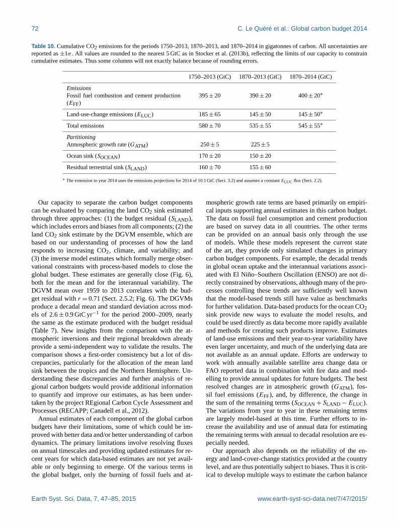
72 C. Le Quéré et al.: Global carbon budget 2014
Table 10. Cumulative CO2 emissions for the periods 1750–2013, 1870–2013, and 1870–2014 in gigatonnes of carbon. All uncertainties are
reported as ±1σ . All values are rounded to the nearest 5 GtC as in Stocker et al. (2013b), reflecting the limits of our capacity to constrain
cumulative estimates. Thus some columns will not exactly balance because of rounding errors.
1750–2013 (GtC) 1870–2013 (GtC) 1870–2014 (GtC)
Emissions
Fossil fuel combustion and cement production
(EFF)
395± 20 390± 20 400± 20∗
Land-use-change emissions (ELUC) 185± 65 145± 50 145± 50∗
Total emissions 580± 70 535± 55 545± 55∗
Partitioning
Atmospheric growth rate (GATM) 250± 5 225± 5
Ocean sink (SOCEAN) 170± 20 150± 20
Residual terrestrial sink (SLAND) 160± 70 155± 60
∗ The extension to year 2014 uses the emissions projections for 2014 of 10.1 GtC (Sect. 3.2) and assumes a constant ELUC flux (Sect. 2.2).
Our capacity to separate the carbon budget components
can be evaluated by comparing the land CO2 sink estimated
through three approaches: (1) the budget residual (SLAND),
which includes errors and biases from all components; (2) the
land CO2 sink estimate by the DGVM ensemble, which are
based on our understanding of processes of how the land
responds to increasing CO2, climate, and variability; and
(3) the inverse model estimates which formally merge obser-
vational constraints with process-based models to close the
global budget. These estimates are generally close (Fig. 6),
both for the mean and for the interannual variability. The
DGVM mean over 1959 to 2013 correlates with the bud-
get residual with r = 0.71 (Sect. 2.5.2; Fig. 6). The DGVMs
produce a decadal mean and standard deviation across mod-
els of 2.6± 0.9 GtC yr−1 for the period 2000–2009, nearly
the same as the estimate produced with the budget residual
(Table 7). New insights from the comparison with the at-
mospheric inversions and their regional breakdown already
provide a semi-independent way to validate the results. The
comparison shows a first-order consistency but a lot of dis-
crepancies, particularly for the allocation of the mean land
sink between the tropics and the Northern Hemisphere. Un-
derstanding these discrepancies and further analysis of re-
gional carbon budgets would provide additional information
to quantify and improve our estimates, as has been under-
taken by the project REgional Carbon Cycle Assessment and
Processes (RECAPP; Canadell et al., 2012).
Annual estimates of each component of the global carbon
budgets have their limitations, some of which could be im-
proved with better data and/or better understanding of carbon
dynamics. The primary limitations involve resolving fluxes
on annual timescales and providing updated estimates for re-
cent years for which data-based estimates are not yet avail-
able or only beginning to emerge. Of the various terms in
the global budget, only the burning of fossil fuels and at-
mospheric growth rate terms are based primarily on empiri-
cal inputs supporting annual estimates in this carbon budget.
The data on fossil fuel consumption and cement production
are based on survey data in all countries. The other terms
can be provided on an annual basis only through the use
of models. While these models represent the current state
of the art, they provide only simulated changes in primary
carbon budget components. For example, the decadal trends
in global ocean uptake and the interannual variations associ-
ated with El Niño–Southern Oscillation (ENSO) are not di-
rectly constrained by observations, although many of the pro-
cesses controlling these trends are sufficiently well known
that the model-based trends still have value as benchmarks
for further validation. Data-based products for the ocean CO2
sink provide new ways to evaluate the model results, and
could be used directly as data become more rapidly available
and methods for creating such products improve. Estimates
of land-use emissions and their year-to-year variability have
even larger uncertainty, and much of the underlying data are
not available as an annual update. Efforts are underway to
work with annually available satellite area change data or
FAO reported data in combination with fire data and mod-
elling to provide annual updates for future budgets. The best
resolved changes are in atmospheric growth (GATM), fos-
sil fuel emissions (EFF), and, by difference, the change in
the sum of the remaining terms (SOCEAN+ SLAND−ELUC).
The variations from year to year in these remaining terms
are largely model-based at this time. Further efforts to in-
crease the availability and use of annual data for estimating
the remaining terms with annual to decadal resolution are es-
pecially needed.
Our approach also depends on the reliability of the en-
ergy and land-cover-change statistics provided at the country
level, and are thus potentially subject to biases. Thus it is crit-
ical to develop multiple ways to estimate the carbon balance
Earth Syst. Sci. Data, 7, 47–85, 2015 www.earth-syst-sci-data.net/7/47/2015/

C. Le Quéré et al.: Global carbon budget 2014 73
at the global and regional level, including estimates from the
inversion of atmospheric CO2 concentration used here for the
first time, the use of other oceanic and atmospheric tracers,
and the compilation of emissions using alternative statistics
(e.g. sectors). It is also important to challenge the consistency
of information across observational streams, for example to
contrast the coherence of temperature trends with those of
CO2 sink trends. Multiple approaches ranging from global
to regional scale would greatly help increase confidence and
reduce uncertainty in CO2 emissions and their fate.
5 Conclusions
The estimation of global CO2 emissions and sinks is a major
effort by the carbon cycle research community that requires a
combination of measurements and compilation of statistical
estimates and results from models. The delivery of an annual
carbon budget serves two purposes. First, there is a large de-
mand for up-to-date information on the state of the anthro-
pogenic perturbation of the climate system and its underpin-
ning causes. A broad stakeholder community relies on the
data sets associated with the annual carbon budget, includ-
ing scientists, policy makers, businesses, journalists, and the
broader society increasingly engaged in adapting to and mit-
igating human-driven climate change. Second, over the last
decade we have seen unprecedented changes in the human
and biophysical environments (e.g. increase in the growth of
fossil fuel emissions, ocean temperatures, and strength of the
land sink), which call for more frequent assessments of the
state of the planet, and by implications a better understanding
of the future evolution of the carbon cycle, and the require-
ments for climate change mitigation and adaptation. Both the
ocean and the land surface presently remove a large fraction
of anthropogenic emissions. Any significant change in the
function of carbon sinks is of great importance to climate pol-
icymaking, as they affect the excess carbon dioxide remain-
ing in the atmosphere and therefore the compatible emissions
for any climate stabilisation target. Better constraints of car-
bon cycle models against contemporary data sets raises the
capacity for the models to become more accurate at future
projections.
This all requires more frequent, robust, and transparent
data sets and methods that can be scrutinised and replicated.
After nine annual releases from the GCP, the effort is grow-
ing and the traceability of the methods has become increas-
ingly complex. Here, we have documented in detail the data
sets and methods used to compile the annual updates of the
global carbon budget, explained the rationale for the choices
made and the limitations of the information, and finally high-
lighted the need for additional information where gaps exist.
This paper, via “living data”, will help to keep track of new
budget updates. The evolution over time of the carbon bud-
get is now a key indicator of the anthropogenic perturbation
of the climate system, and its annual delivery joins a set of
other climate indicators to monitor the evolution of human-
induced climate change, such as the annual updates on the
global surface temperature, sea level rise, minimum Arctic
sea ice extent, and others.
Data access
The data presented here are made available in the belief that
their wide dissemination will lead to greater understanding
and new scientific insights into how the carbon cycle works,
how humans are altering it, and how we can mitigate the re-
sulting human-driven climate change. The free availability of
these data does not constitute permission for publication of
the data. For research projects, if the data are essential to the
work, or if an important result or conclusion depends on the
data, co-authorship may need to be considered. Full contact
details and information on how to cite the data are given at
the top of each page in the accompanying database and sum-
marised in Table 2.
The accompanying database includes an Excel file or-
ganised in the following spreadsheets (accessible with
the free viewer http://www.microsoft.com/en-us/download/
details.aspx?id=10):
1. Summary;
2. The global carbon budget (1959–2013);
3. Global CO2 emissions from fossil fuel combustion and
cement production by fuel type, and the per capita emis-
sions (1959–2013);
4. Territorial (e.g. as reported to the UN Framework Con-
vention on Climate Change) country CO2 emissions
from fossil fuel combustion and cement production
(1959–2013);
5. Consumption country CO2 emissions from fossil fuel
combustion and cement production and emissions trans-
fer from the international trade of goods and services
(1990–2012);
6. Emissions transfers (consumption minus territorial
emissions; 1990–2012);
7. CO2 emissions from land-use change from the individ-
ual methods and models (1959–2013);
8. Ocean CO2 sink from the individual ocean models and
data products (1959–2013);
9. Terrestrial residual CO2 sink from the DGVMs (1959–
2013);
10. Additional information on the carbon balance prior to
1959 (1750–2013);
11. Country definitions.
www.earth-syst-sci-data.net/7/47/2015/ Earth Syst. Sci. Data, 7, 47–85, 2015

74 C. Le Quéré et al.: Global carbon budget 2014
Appendix A: Additional ocean data combined with
SOCATv2 and used by the ocean data products
Table A1. Attribution of fCO2 measurements for years 2012–2013 used in addition to SOCAT v2 (Bakker et al., 2014) to inform ocean
data products.
Start date End date Regions No. of samples Principal investigators DOI (if available)
2012-07-16 2012-07-29 Arctic 12 773 Hoppema, M., and S. van Heuven
2012-01-25 2012-03-07 Indian Ocean,
Southern Ocean
6939 Metzl, N. doi:10.3334/CDIAC/OTG.VOS_OISO_21
2013-02-10 2013-03-09 Indian Ocean,
Southern Ocean
2220 Metzl, N. doi:10.3334/CDIAC/OTG.VOS_OISO_22
2012-01-10 2012-01-20 North Atlantic 2989 Johannessen, T., A. Omar, and I. Skjelvan
2012-01-11 2012-01-11 North Atlantic 1360 Vandemark, D., J. Salisbury, R. Morrison, C. Hunt, and W. McGillis doi:10.3334/CDIAC/otg.TSM_UNH_GOM
2012-02-07 2012-02-07 North Atlantic 1912 Vandemark, D., J. Salisbury, R. Morrison, C. Hunt, and W. McGillis doi:10.3334/CDIAC/otg.TSM_UNH_GOM
2012-02-07 2012-02-17 North Atlantic 3115 Johannessen, T., A. Omar, and I. Skjelvan
2012-02-18 2012-02-25 North Atlantic 2693 Johannessen, T., A. Omar, and I. Skjelvan
2012-02-22 2012-03-01 North Atlantic 5099 Bozec, Y.
2012-02-27 2012-03-26 North Atlantic 9360 Wanninkhof, R., K. Sullivan, J. Hare, and C. Taylor doi:10.3334/CDIAC/OTG.AOML_BIGELOW_ECOAST_2011_2012
2012-02-29 2013-02-18 North Atlantic 2842 Sutton, A., J. Mathis, C. Sabine, S. Musielewicz, and S. Maenner doi:10.3334/CDIAC/OTG.TSM_Crescent_64W_32N
2012-02-29 2013-03-15 North Atlantic 2888 Sutton, A., J. Mathis, C. Sabine, S. Musielewicz, and S. Maenner doi:10.3334/CDIAC/OTG.TSM_Hog_Reef_64W_32N
2012-03-01 2012-03-12 North Atlantic 4867 Lauvset, S. and T. Johannessen
2012-03-13 2012-03-19 North Atlantic 2235 Johannessen, T., A. Omar, and I. Skjelvan
2012-03-17 2012-03-19 North Atlantic 976 Lauvset, S. and T. Johannessen
2012-03-17 2012-03-22 North Atlantic 6358 Steinhoff, T., M. Becker, and A. Körtzinger doi:10.3334/CDIAC/OTG.VOS_Atlantic_Companion_Line_2012
2012-03-22 2012-03-29 North Atlantic 2304 Johannessen, T., A. Omar, and I. Skjelvan
2012-04-02 2012-05-04 North Atlantic 12 318 Wanninkhof, R., K. Sullivan, J. Hare, and C. Taylor doi:10.3334/CDIAC/OTG.AOML_BIGELOW_ECOAST_2011_2012
2012-04-06 2012-04-06 North Atlantic 1201 Vandemark, D., J. Salisbury, R. Morrison, C. Hunt, and W. McGillis doi:10.3334/CDIAC/otg.TSM_UNH_GOM
2012-04-06 2012-04-11 North Atlantic 3367 Steinhoff, T., M. Becker, and A. Körtzinger doi:10.3334/CDIAC/OTG.VOS_Atlantic_Companion_Line_2012
2012-04-07 2012-04-12 North Atlantic 1572 Wanninkhof, R., B. Huss, R. Castle doi:10.3334/CDIAC/OTG.VOS_EXP2012
2012-04-13 2012-04-21 North Atlantic 2994 Johannessen, T., A. Omar, and I. Skjelvan
2012-04-20 2012-04-26 North Atlantic 6321 Steinhoff, T., M. Becker, and A. Körtzinger doi:10.3334/CDIAC/OTG.VOS_Atlantic_Companion_Line_2012
2012-04-22 2012-04-27 North Atlantic 1492 Johannessen, T., A. Omar, and I. Skjelvan
2012-04-25 2012-04-26 North Atlantic 419 Wanninkhof, R., B. Huss, R. Castle doi:10.3334/CDIAC/OTG.VOS_EXP2012
2012-05-02 2012-05-08 North Atlantic 484 Johannessen, T., A. Omar, and I. Skjelvan
2012-05-05 2012-05-10 North Atlantic 1422 Wanninkhof, R., B. Huss, R. Castle doi:10.3334/CDIAC/OTG.VOS_EXP2012
2012-05-11 2012-05-15 North Atlantic 4544 Steinhoff, T., M. Becker, and A. Körtzinger doi:10.3334/CDIAC/OTG.VOS_Atlantic_Companion_Line_2012
2012-05-19 2012-05-24 North Atlantic 1567 Wanninkhof, R., B. Huss, R. Castle doi:10.3334/CDIAC/OTG.VOS_EXP2012
2012-05-25 2012-05-31 North Atlantic 7969 Steinhoff, T., M. Becker, and A. Körtzinger doi:10.3334/CDIAC/OTG.VOS_Atlantic_Companion_Line_2012
2012-05-31 2012-06-14 North Atlantic 5472 Wanninkhof, R., K. Sullivan, J. Hare, and C. Taylor doi:10.3334/CDIAC/OTG.AOML_BIGELOW_ECOAST_2011_2012
2012-06-02 2012-06-07 North Atlantic 1568 Wanninkhof, R., B. Huss, R. Castle doi:10.3334/CDIAC/OTG.VOS_EXP2012
2012-06-11 2012-06-11 North Atlantic 1085 Vandemark, D., J. Salisbury, R. Morrison, C. Hunt, and W. McGillis doi:10.3334/CDIAC/otg.TSM_UNH_GOM
2012-06-16 2012-06-21 North Atlantic 1534 Wanninkhof, R., B. Huss, R. Castle doi:10.3334/CDIAC/OTG.VOS_EXP2012
2012-06-18 2012-06-28 North Atlantic 5370 Wanninkhof, R., K. Sullivan, J. Hare, and C. Taylor doi:10.3334/CDIAC/OTG.AOML_BIGELOW_ECOAST_2011_2012
2012-06-29 2012-07-03 North Atlantic 6134 Steinhoff, T., M. Becker, and A. Körtzinger doi:10.3334/CDIAC/OTG.VOS_Atlantic_Companion_Line_2012
2012-06-30 2012-07-05 North Atlantic 1590 Wanninkhof, R., B. Huss, R. Castle doi:10.3334/CDIAC/OTG.VOS_EXP2012
2012-07-03 2012-07-03 North Atlantic 1367 Vandemark, D., J. Salisbury, R. Morrison, C. Hunt, and W. McGillis doi:10.3334/CDIAC/otg.TSM_UNH_GOM
2012-07-06 2012-07-18 North Atlantic 6216 Wanninkhof, R., K. Sullivan, J. Hare, and C. Taylor doi:10.3334/CDIAC/OTG.AOML_BIGELOW_ECOAST_2011_2012
2012-07-14 2012-07-19 North Atlantic 1595 Wanninkhof, R., B. Huss, R. Castle doi:10.3334/CDIAC/OTG.VOS_EXP2012
2012-07-16 2012-07-20 North Atlantic 6960 Steinhoff, T., M. Becker, and A. Körtzinger doi:10.3334/CDIAC/OTG.VOS_Atlantic_Companion_Line_2012
2012-07-20 2012-07-27 North Atlantic 5399 Bozec, Y.
2012-07-25 2012-08-01 North Atlantic 26 Johannessen, T., A. Omar, and I. Skjelvan
2012-07-28 2012-08-02 North Atlantic 1584 Wanninkhof, R., B. Huss, R. Castle doi:10.3334/CDIAC/OTG.VOS_EXP2012
2012-08-02 2012-08-07 North Atlantic 6332 Steinhoff, T., M. Becker, and A. Körtzinger doi:10.3334/CDIAC/OTG.VOS_Atlantic_Companion_Line_2012
2012-08-07 2012-08-24 North Atlantic 9092 Wanninkhof, R., K. Sullivan, J. Hare, and C. Taylor doi:10.3334/CDIAC/OTG.AOML_BIGELOW_ECOAST_2011_2012
2012-08-19 2012-08-27 North Atlantic 4036 Wanninkhof, R., R. D. Castle, and J. Shannahoff doi:10.3334/CDIAC/OTG.VOS_RB_2012
2012-08-22 2013-07-09 North Atlantic 2574 Mathis, J., A. Sutton, C. Sabine, S. Musielewicz, and S. Maenner doi:10.3334/CDIAC/OTG.TSM_NH_70W_43N
2012-08-23 2012-08-24 North Atlantic 246 Johannessen, T., A. Omar, and I. Skjelvan
2012-08-25 2012-08-28 North Atlantic 221 Johannessen, T., A. Omar, and I. Skjelvan
2012-08-25 2012-08-30 North Atlantic 1602 Wanninkhof, R., B. Huss, R. Castle doi:10.3334/CDIAC/OTG.VOS_EXP2012
2012-08-30 2012-09-03 North Atlantic 10 930 Schuster, U. and A. J. Watson
2012-09-05 2012-09-16 North Atlantic 412 Johannessen, T., A. Omar, and I. Skjelvan
2012-09-13 2012-09-13 North Atlantic 1876 Vandemark, D., J. Salisbury, R. Morrison, C. Hunt, and W. McGillis doi:10.3334/CDIAC/otg.TSM_UNH_GOM
2012-09-14 2012-09-14 North Atlantic 1265 Vandemark, D., J. Salisbury, R. Morrison, C. Hunt, and W. McGillis doi:10.3334/CDIAC/otg.TSM_UNH_GOM
2012-09-17 2012-09-18 North Atlantic 305 Johannessen, T., A. Omar, and I. Skjelvan
2012-09-19 2013-01-22 North Atlantic 911 Mathis, J., A. Sutton, C. Sabine, S. Musielewicz, and S. Maenner doi:10.3334/CDIAC/OTG.TSM_GRAYSRF_81W_31N
2012-09-24 2012-09-30 North Atlantic 7453 Steinhoff, T., M. Becker, and A. Körtzinger doi:10.3334/CDIAC/OTG.VOS_Atlantic_Companion_Line_2012
2012-09-26 2012-10-01 North Atlantic 15 120 Schuster, U. and A. J. Watson
2012-09-26 2012-10-06 North Atlantic 650 Johannessen, T., A. Omar, and I. Skjelvan
2012-10-07 2012-10-08 North Atlantic 237 Wanninkhof, R., B. Huss, R. Castle doi:10.3334/CDIAC/OTG.VOS_EXP2012
2012-10-07 2012-10-13 North Atlantic 527 Johannessen, T., A. Omar, and I. Skjelvan
2012-10-10 2012-10-16 North Atlantic 6509 Steinhoff, T., M. Becker, and A. Körtzinger doi:10.3334/CDIAC/OTG.VOS_Atlantic_Companion_Line_2012
2012-10-14 2012-10-21 North Atlantic 1263 Wanninkhof, R., B. Huss, R. Castle doi:10.3334/CDIAC/OTG.VOS_EXP2012
2012-10-21 2012-10-28 North Atlantic 1839 Wanninkhof, R., B. Huss, R. Castle doi:10.3334/CDIAC/OTG.VOS_EXP2012
2012-10-27 2012-10-30 North Atlantic 4231 Steinhoff, T., M. Becker, and A. Körtzinger doi:10.3334/CDIAC/OTG.VOS_Atlantic_Companion_Line_2012
2012-10-28 2012-11-04 North Atlantic 520 Wanninkhof, R., B. Huss, R. Castle doi:10.3334/CDIAC/OTG.VOS_EXP2012
2012-11-06 2012-11-06 North Atlantic 1087 Vandemark, D., J. Salisbury, R. Morrison, C. Hunt, and W. McGillis doi:10.3334/CDIAC/otg.TSM_UNH_GOM
2012-11-07 2012-11-17 North Atlantic 2464 Johannessen, T., A. Omar, and I. Skjelvan
2012-11-15 2012-11-16 North Atlantic 288 Wanninkhof, R., B. Huss, R. Castle doi:10.3334/CDIAC/OTG.VOS_EXP2012
2012-11-17 2012-11-26 North Atlantic 3067 Johannessen, T., A. Omar, and I. Skjelvan
2012-11-28 2012-12-04 North Atlantic 1021 Johannessen, T., A. Omar, and I. Skjelvan
2012-11-29 2012-12-05 North Atlantic 10 018 Steinhoff, T., M. Becker, and A. Körtzinger doi:10.3334/CDIAC/OTG.VOS_Atlantic_Companion_Line_2012
2012-12-09 2012-12-17 North Atlantic 2791 Johannessen, T., A. Omar, and I. Skjelvan
2012-12-12 2012-12-13 North Atlantic 3020 Schuster, U. and A. J. Watson
2012-12-29 2013-01-05 North Atlantic 2739 Omar, A., A. Olsen, and T. Johannessen
2013-01-08 2013-01-13 North Atlantic 15 570 Schuster, U. and A. J. Watson
2013-02-01 2013-02-09 North Atlantic 2527 Omar, A., A. Olsen, and T. Johannessen
Earth Syst. Sci. Data, 7, 47–85, 2015 www.earth-syst-sci-data.net/7/47/2015/

C. Le Quéré et al.: Global carbon budget 2014 75
Table A1. Continued.
Start date End date Regions No. of samples Principal investigators DOI (if available)
2013-02-12 2013-02-16 North Atlantic 6134 Steinhoff, T. and A. Körtzinger
2013-02-12 2013-02-21 North Atlantic 2834 Omar, A., A. Olsen, and T. Johannessen
2013-02-21 2013-03-01 North Atlantic 2724 Omar, A., A. Olsen, and T. Johannessen
2013-03-05 2013-03-12 North Atlantic 2553 Omar, A., A. Olsen, and T. Johannessen
2013-03-14 2013-05-09 North Atlantic 22 913 Wanninkhof, R., K. Sullivan, J. Hare, and C. Taylor doi:10.3334/CDIAC/OTG.AOML_BIGELOW_ECOAST_2013
2013-03-21 2013-03-26 North Atlantic 6894 Steinhoff, T., and A. Körtzinger
2013-04-15 2013-04-15 North Atlantic 1186 Vandemark, D., J. Salisbury, R. Morrison, C. Hunt, and W. McGillis doi:10.3334/CDIAC/otg.TSM_UNH_GOM
2013-04-16 2013-04-26 North Atlantic 3365 Omar, A., A. Olsen, and T. Johannessen
2013-04-27 2013-05-02 North Atlantic 397 Wanninkhof, R., B. Huss, K. Sullivan, and R. Castle doi:10.3334/CDIAC/OTG.VOS_EXP2013
2013-05-06 2013-05-11 North Atlantic 6362 Steinhoff, T., and A. Körtzinger
2013-05-21 2013-05-21 North Atlantic 1216 Vandemark, D., J. Salisbury, R. Morrison, C. Hunt, and W. McGillis doi:10.3334/CDIAC/otg.TSM_UNH_GOM
2013-05-29 2013-06-06 North Atlantic 2122 Omar, A., A. Olsen, and T. Johannessen
2013-06-07 2013-06-12 North Atlantic 1312 Omar, A., A. Olsen, and T. Johannessen
2013-06-12 2013-06-24 North Atlantic 4620 Wanninkhof, R., K. Sullivan, J. Hare, and C. Taylor doi:10.3334/CDIAC/OTG.AOML_BIGELOW_ECOAST_2013
2013-06-18 2013-06-21 North Atlantic 426 Omar, A., A. Olsen, and T. Johannessen
2013-07-01 2013-08-18 North Atlantic 16 824 Wanninkhof, R., K. Sullivan, J. Hare, and C. Taylor doi:10.3334/CDIAC/OTG.AOML_BIGELOW_ECOAST_2013
2013-07-10 2013-07-19 North Atlantic 300 Omar, A., A. Olsen, and T. Johannessen
2013-07-18 2013-07-28 North Atlantic 4986 Wanninkhof, R., R. D. Castle, and J. Shannahoff doi:10.3334/CDIAC/OTG.VOS_RB_2013
2013-07-19 2013-07-23 North Atlantic 1033 Omar, A., A. Olsen, and T. Johannessen
2013-08-15 2013-08-15 North Atlantic 735 Vandemark, D., J. Salisbury, R. Morrison, C. Hunt, and W. McGillis doi:10.3334/CDIAC/otg.TSM_UNH_GOM
2013-09-03 2013-11-19 North Atlantic 23 184 Wanninkhof, R., K. Sullivan, J. Hare, and C. Taylor doi:10.3334/CDIAC/OTG.AOML_BIGELOW_ECOAST_2013
2013-09-11 2013-09-17 North Atlantic 1770 Omar, A., A. Olsen, and T. Johannessen
2013-09-18 2013-09-24 North Atlantic 6691 Steinhoff, T., and A. Körtzinger
2013-10-01 2013-10-06 North Atlantic 962 Wanninkhof, R., B. Huss, K. Sullivan, and R. Castle doi:10.3334/CDIAC/OTG.VOS_EXP2013
2013-10-04 2013-10-09 North Atlantic 5928 Steinhoff, T., and A. Körtzinger
2013-10-22 2013-10-31 North Atlantic 2814 Omar, A., A. Olsen, and T. Johannessen
2013-10-27 2013-11-03 North Atlantic 1836 Wanninkhof, R., B. Huss, K. Sullivan, and R. Castle doi:10.3334/CDIAC/OTG.VOS_EXP2013
2013-11-01 2013-11-10 North Atlantic 2232 Omar, A., A. Olsen, and T. Johannessen
2013-11-02 2013-11-06 North Atlantic 3756 Steinhoff, T., and A. Körtzinger
2013-11-18 2013-11-23 North Atlantic 5878 Steinhoff, T., and A. Körtzinger
2013-11-22 2013-11-24 North Atlantic 360 Omar, A., A. Olsen, and T. Johannessen
2013-11-24 2013-12-01 North Atlantic 2251 Omar, A., A. Olsen, and T. Johannessen
2013-12-05 2013-12-11 North Atlantic 2219 Omar, A., A. Olsen, and T. Johannessen
2013-12-22 2013-12-23 North Atlantic 309 Wanninkhof, R., B. Huss, K. Sullivan, and R. Castle doi:10.3334/CDIAC/OTG.VOS_EXP2013
2013-12-28 2013-12-31 North Atlantic 1006 Omar, A., A. Olsen, and T. Johannessen
2012-06-15 2012-07-14 North Atlantic, Arctic 28 783 Hoppema, M., and S. van Heuven
2012-07-02 2012-07-20 North Atlantic, Arctic 8265 Lauvset, S. and T. Johannessen
2012-07-23 2012-08-13 North Atlantic, Arctic 7910 Lauvset, S. and T. Johannessen
2012-08-03 2012-10-06 North Atlantic, Arctic 63 105 Hoppema, M., and S. van Heuven
2013-07-15 2013-08-16 North Atlantic, Arctic 2212 Kitidis, V. doi:10.3334/CDIAC/OTG.VOS_JCR_2013
2013-08-20 2013-08-30 North Atlantic, Arctic 3150 Omar, A., A. Olsen, and T. Johannessen
2013-09-01 2013-09-09 North Atlantic, Arctic 3120 Omar, A., A. Olsen, and T. Johannessen
2012-01-07 2012-01-15 North Atlantic, tropical Atlantic 20 416 Schuster, U. and A. J. Watson
2012-01-29 2012-02-06 North Atlantic, tropical Atlantic 2699 Wanninkhof, R., B. Huss, R. Castle doi:10.3334/CDIAC/OTG.VOS_EXP2012
2012-02-05 2012-02-10 North Atlantic, tropical Atlantic 12 650 Schuster, U. and A. J. Watson
2012-02-06 2012-02-17 North Atlantic, tropical Atlantic 4082 Wanninkhof, R., B. Huss, R. Castle doi:10.3334/CDIAC/OTG.VOS_EXP2012
2012-02-16 2012-03-05 North Atlantic, tropical Atlantic 8951 Wanninkhof, R., R. D. Castle, and J. Shannahoff doi:10.3334/CDIAC/OTG.VOS_RB_2012
2012-02-17 2012-02-27 North Atlantic, tropical Atlantic 3988 Wanninkhof, R., B. Huss, R. Castle doi:10.3334/CDIAC/OTG.VOS_EXP2012
2012-02-27 2012-03-09 North Atlantic, tropical Atlantic 4214 Wanninkhof, R., B. Huss, R. Castle doi:10.3334/CDIAC/OTG.VOS_EXP2012
2012-03-09 2012-03-19 North Atlantic, tropical Atlantic 4127 Wanninkhof, R., B. Huss, R. Castle doi:10.3334/CDIAC/OTG.VOS_EXP2012
2012-03-17 2012-03-21 North Atlantic, tropical Atlantic 13 144 Schuster, U. and A. J. Watson
2012-03-19 2012-03-30 North Atlantic, tropical Atlantic 4283 Wanninkhof, R., B. Huss, R. Castle doi:10.3334/CDIAC/OTG.VOS_EXP2012
2012-03-30 2012-04-07 North Atlantic, tropical Atlantic 2642 Wanninkhof, R., B. Huss, R. Castle doi:10.3334/CDIAC/OTG.VOS_EXP2012
2012-04-11 2012-04-19 North Atlantic, tropical Atlantic 18 433 Schuster, U. and A. J. Watson
2012-04-12 2012-04-21 North Atlantic, tropical Atlantic 3510 Wanninkhof, R., B. Huss, R. Castle doi:10.3334/CDIAC/OTG.VOS_EXP2012
2012-04-26 2012-05-05 North Atlantic, tropical Atlantic 3386 Wanninkhof, R., B. Huss, R. Castle doi:10.3334/CDIAC/OTG.VOS_EXP2012
2012-04-28 2012-05-06 North Atlantic, tropical Atlantic 18 194 Schuster, U. and A. J. Watson
2012-05-09 2012-05-16 North Atlantic, tropical Atlantic 18 800 Schuster, U. and A. J. Watson
2012-05-10 2012-05-19 North Atlantic, tropical Atlantic 3615 Wanninkhof, R., B. Huss, R. Castle doi:10.3334/CDIAC/OTG.VOS_EXP2012
2012-05-24 2012-06-02 North Atlantic, tropical Atlantic 3637 Wanninkhof, R., B. Huss, R. Castle doi:10.3334/CDIAC/OTG.VOS_EXP2012
2012-05-26 2012-06-03 North Atlantic, tropical Atlantic 22 839 Schuster, U. and A. J. Watson
2012-06-07 2012-06-16 North Atlantic, tropical Atlantic 3568 Wanninkhof, R., B. Huss, R. Castle doi:10.3334/CDIAC/OTG.VOS_EXP2012
2012-06-21 2012-06-30 North Atlantic, tropical Atlantic 3596 Wanninkhof, R., B. Huss, R. Castle doi:10.3334/CDIAC/OTG.VOS_EXP2012
2012-07-03 2012-07-15 North Atlantic, tropical Atlantic 6385 Wanninkhof, R., R. D. Castle, and J. Shannahoff doi:10.3334/CDIAC/OTG.VOS_RB_2012
2012-07-04 2012-07-12 North Atlantic, tropical Atlantic 18 898 Schuster, U. andA. J. Watson
2012-07-05 2012-07-14 North Atlantic, tropical Atlantic 3608 Wanninkhof, R., B. Huss, R. Castle doi:10.3334/CDIAC/OTG.VOS_EXP2012
2012-07-19 2012-07-28 North Atlantic, tropical Atlantic 3577 Wanninkhof, R., B. Huss, R. Castle doi:10.3334/CDIAC/OTG.VOS_EXP2012
2012-08-01 2012-08-09 North Atlantic, tropical Atlantic 18 038 Schuster, U. and A. J. Watson
2012-08-02 2012-08-08 North Atlantic, tropical Atlantic 2308 Wanninkhof, R., B. Huss, R. Castle doi:10.3334/CDIAC/OTG.VOS_EXP2012
2012-08-16 2012-08-25 North Atlantic, tropical Atlantic 3149 Wanninkhof, R., B. Huss, R. Castle doi:10.3334/CDIAC/OTG.VOS_EXP2012
2012-08-30 2012-09-04 North Atlantic, tropical Atlantic 1745 Wanninkhof, R., B. Huss, R. Castle doi:10.3334/CDIAC/OTG.VOS_EXP2012
2012-10-24 2012-11-01 North Atlantic, tropical Atlantic 24 050 Schuster, U. andA. J. Watson
2012-11-04 2012-11-15 North Atlantic, tropical Atlantic 3438 Wanninkhof, R., B. Huss, R. Castle doi:10.3334/CDIAC/OTG.VOS_EXP2012
2012-11-21 2012-11-29 North Atlantic, tropical Atlantic 25 485 Schuster, U. and A. J. Watson
2012-12-20 2012-12-26 North Atlantic, tropical Atlantic 19 097 Schuster, U. and A. J. Watson
2013-01-16 2013-01-21 North Atlantic, tropical Atlantic 14 524 Schuster, U. and A. J. Watson
2013-02-02 2013-02-08 North Atlantic, tropical Atlantic 12 706 Schuster, U. and A. J. Watson
2013-02-14 2013-02-21 North Atlantic, tropical Atlantic 21 740 Schuster, U. and A. J. Watson
2013-03-02 2013-03-10 North Atlantic, tropical Atlantic 26 110 Schuster, U. and A. J. Watson
2013-04-22 2013-04-27 North Atlantic, tropical Atlantic 1754 Wanninkhof, R., B. Huss, K. Sullivan, and R. Castle doi:10.3334/CDIAC/OTG.VOS_EXP2013
2013-05-02 2013-05-11 North Atlantic, tropical Atlantic 746 Wanninkhof, R., B. Huss, K. Sullivan, and R. Castle doi:10.3334/CDIAC/OTG.VOS_EXP2013
2013-05-04 2013-05-09 North Atlantic, tropical Atlantic 14 790 Schuster, U. and A. J. Watson
2013-05-16 2013-05-25 North Atlantic, tropical Atlantic 1095 Wanninkhof, R., B. Huss, K. Sullivan, and R. Castle doi:10.3334/CDIAC/OTG.VOS_EXP2013
2013-05-18 2013-05-26 North Atlantic, tropical Atlantic 23 850 Schuster, U. and A. J. Watson
2013-05-30 2013-06-06 North Atlantic, tropical Atlantic 20 750 Schuster, U. and A. J. Watson
2013-06-15 2013-06-23 North Atlantic, tropical Atlantic 23 000 Schuster, U. and A. J. Watson
2013-06-26 2013-07-04 North Atlantic, tropical Atlantic 22 820 Schuster, U. and A. J. Watson
2013-07-13 2013-07-21 North Atlantic, tropical Atlantic 23 240 Schuster, U. and A. J. Watson
2013-07-24 2013-08-01 North Atlantic, tropical Atlantic 22 420 Schuster, U. and A. J. Watson
2013-08-03 2013-10-02 North Atlantic, tropical Atlantic 25 325 Wanninkhof, R., R. D. Castle, and J. Shannahoff doi:10.3334/CDIAC/OTG.VOS_RB_2013
2013-08-10 2013-08-18 North Atlantic, tropical Atlantic 22 550 Schuster, U. and A. J. Watson
2013-08-21 2013-08-29 North Atlantic, tropical Atlantic 22 910 Schuster, U. and A. J. Watson
2013-09-07 2013-09-15 North Atlantic, tropical Atlantic 22 950 Schuster, U. and A. J. Watson
2013-09-18 2013-09-27 North Atlantic, tropical Atlantic 26 010 Schuster, U. and A. J. Watson
2013-10-05 2013-10-13 North Atlantic, tropical Atlantic 23 780 Schuster, U. and A. J. Watson
www.earth-syst-sci-data.net/7/47/2015/ Earth Syst. Sci. Data, 7, 47–85, 2015

76 C. Le Quéré et al.: Global carbon budget 2014
Table A1. Continued.
Start date End date Regions No. of samples Principal investigators DOI (if available)
2013-10-16 2013-10-24 North Atlantic, tropical Atlantic 22 330 Schuster, U. and A. J. Watson
2013-11-02 2013-11-10 North Atlantic, tropical Atlantic 23 040 Schuster, U. and A. J. Watson
2013-11-03 2013-11-14 North Atlantic, tropical Atlantic 3847 Wanninkhof, R., B. Huss, K. Sullivan, and R. Castle doi:10.3334/CDIAC/OTG.VOS_EXP2013
2013-11-13 2013-11-20 North Atlantic, tropical Atlantic 20 720 Schuster, U. and A. J. Watson
2013-11-14 2013-11-23 North Atlantic, tropical Atlantic 3136 Wanninkhof, R., B. Huss, K. Sullivan, and R. Castle doi:10.3334/CDIAC/OTG.VOS_EXP2013
2013-11-23 2013-12-02 North Atlantic, tropical Atlantic 2476 Wanninkhof, R., B. Huss, K. Sullivan, and R. Castle doi:10.3334/CDIAC/OTG.VOS_EXP2013
2013-11-30 2013-12-08 North Atlantic, tropical Atlantic 23 980 Schuster, U. and A. J. Watson
2013-12-02 2013-12-12 North Atlantic, tropical Atlantic 3402 Wanninkhof, R., B. Huss, K. Sullivan, and R. Castle doi:10.3334/CDIAC/OTG.VOS_EXP2013
2013-12-12 2013-12-22 North Atlantic, tropical Atlantic 4082 Wanninkhof, R., B. Huss, K. Sullivan, and R. Castle doi:10.3334/CDIAC/OTG.VOS_EXP2013
2012-06-14 2012-07-11 North Atlantic, tropical Atlantic,
North Pacific, tropical Pacific
3955 Nojiri, Y. doi:10.3334/CDIAC/otg.VOS_Pyxis_Lines
2012-04-11 2012-05-14 North Atlantic, tropical Atlantic,
Southern Ocean
31 606 Hoppema, M., and S. van Heuven
2012-01-16 2012-01-16 North Pacific 94 Nojiri, Y. doi:10.3334/CDIAC/OTG.VOS_TF5_2012
2012-01-18 2012-01-22 North Pacific 712 Nojiri, Y. doi:10.3334/CDIAC/OTG.VOS_TF5_2012
2012-02-02 2012-02-16 North Pacific 2032 Nojiri, Y. doi:10.3334/CDIAC/otg.VOS_Pyxis_Lines
2012-02-03 2012-02-04 North Pacific 162 Nojiri, Y. doi:10.3334/CDIAC/OTG.VOS_TF5_2012
2012-02-15 2012-02-15 North Pacific 85 Nojiri, Y. doi:10.3334/CDIAC/OTG.VOS_TF5_2012
2012-02-17 2012-02-17 North Pacific 89 Nojiri, Y. doi:10.3334/CDIAC/OTG.VOS_TF5_2012
2012-02-20 2012-03-01 North Pacific 3184 Cosca, C., R. Feely, S. Alin, and G. Lebon doi:10.3334/CDIAC/otg.VOS_Bell_Shimada/BS_2012
2012-03-03 2012-03-18 North Pacific 2192 Nojiri, Y. doi:10.3334/CDIAC/otg.VOS_Pyxis_Lines
2012-03-24 2013-03-18 North Pacific 2877 Mathis, J., A. Sutton, C. Sabine, S. Musielewicz, and S. Maenner doi:10.3334/CDIAC/otg.TSM_CCE2_121W_34N
2012-03-26 2012-03-27 North Pacific 86 Nojiri, Y. doi:10.3334/CDIAC/OTG.VOS_TF5_2012
2012-03-31 2012-03-31 North Pacific 91 Nojiri, Y. doi:10.3334/CDIAC/OTG.VOS_TF5_2012
2012-04-12 2012-04-21 North Pacific 1353 Saito, S., and A. Nakadate doi:10.3334/CDIAC/OTG.VOS_KeifuMaru_2001_2012
2012-04-18 2012-05-01 North Pacific 1918 Nojiri, Y. doi:10.3334/CDIAC/otg.VOS_Pyxis_Lines
2012-05-02 2012-05-13 North Pacific 1504 Nojiri, Y. doi:10.3334/CDIAC/otg.VOS_Pyxis_Lines
2012-05-07 2012-05-08 North Pacific 87 Nojiri, Y. doi:10.3334/CDIAC/OTG.VOS_TF5_2012
2012-05-11 2012-05-11 North Pacific 83 Nojiri, Y. doi:10.3334/CDIAC/OTG.VOS_TF5_2012
2012-05-16 2012-05-29 North Pacific 1914 Nojiri, Y. doi:10.3334/CDIAC/otg.VOS_Pyxis_Lines
2012-05-22 2012-06-18 North Pacific 30 171 Ono, T., and T. Ichikawa doi:10.3334/CDIAC/OTG.FRA_SY2012
2012-05-26 2013-01-18 North Pacific 1964 Mathis, J., A. Sutton, C. Sabine, S. Musielewicz, S. Maenner, and
R. Bott
doi:10.3334/CDIAC/otg.TSM_LaPush_125W_48N
2012-05-30 2012-06-10 North Pacific 1599 Nojiri, Y. doi:10.3334/CDIAC/otg.VOS_Pyxis_Lines
2012-06-02 2012-06-12 North Pacific 1185 Saito, S., and A. Nakadate doi:10.3334/CDIAC/OTG.VOS_KeifuMaru_2001_2012
2012-06-15 2012-07-07 North Pacific 9030 Takahashi, T., C. Sweeney, and S. C. Sutherland doi:10.3334/CDIAC/OTG.VOS_MG_LANGSETH_LINES
2012-06-18 2012-06-18 North Pacific 85 Nojiri, Y. doi:10.3334/CDIAC/OTG.VOS_TF5_2012
2012-06-22 2012-06-22 North Pacific 89 Nojiri, Y. doi:10.3334/CDIAC/OTG.VOS_TF5_2012
2012-06-25 2012-07-08 North Pacific 17 941 Ono, T., and T. Ichikawa doi:10.3334/CDIAC/OTG.FRA_WK2012
2012-07-12 2012-07-24 North Pacific 4805 Takahashi, T., C. Sweeney, and S. C. Sutherland doi:10.3334/CDIAC/OTG.VOS_MG_LANGSETH_LINES
2012-07-12 2012-09-29 North Pacific 520 Mathis, J., A. Sutton, C. Sabine, S. Musielewicz, and S. Maenner doi:10.3334/CDIAC/OTG.TSM_Dabob_122W_478N
2012-07-17 2012-07-26 North Pacific 4363 Cosca, C., R. Feely, S. Alin, and G. Lebon doi:10.3334/CDIAC/otg.VOS_Bell_Shimada/BS_2012
2012-07-26 2012-09-10 North Pacific 4722 Saito, S., and A. Nakadate doi:10.3334/CDIAC/OTG.VOS_Ryofu_Maru_2010_2013
2012-07-29 2012-08-06 North Pacific 1185 Nojiri, Y. doi:10.3334/CDIAC/otg.VOS_Pyxis_Lines
2012-07-30 2012-07-30 North Pacific 33 Nojiri, Y. doi:10.3334/CDIAC/OTG.VOS_TF5_2012
2012-07-30 2012-08-04 North Pacific 1968 Takahashi, T., C. Sweeney, and S. C. Sutherland doi:10.3334/CDIAC/otg.VOS_CGC_Healy_Lines
2012-08-03 2012-08-03 North Pacific 88 Nojiri, Y. doi:10.3334/CDIAC/OTG.VOS_TF5_2012
2012-08-09 2013-09-05 North Pacific 3062 Mathis, J., A. Sutton, C. Sabine, S. Musielewicz, and S. Maenner doi:10.3334/CDIAC/OTG.TSM_WA_125W_47N
2012-08-13 2012-08-25 North Pacific 1792 Nojiri, Y. doi:10.3334/CDIAC/otg.VOS_Pyxis_Lines
2012-08-17 2012-08-26 North Pacific 3710 Takahashi, T., C. Sweeney, and S. C. Sutherland doi:10.3334/CDIAC/OTG.VOS_MG_LANGSETH_LINES
2012-08-27 2012-09-08 North Pacific 1745 Nojiri, Y. doi:10.3334/CDIAC/otg.VOS_Pyxis_Lines
2012-09-05 2012-09-17 North Pacific 5637 Cosca, C., R. Feely, S. Alin, and G. Lebon doi:10.3334/CDIAC/otg.VOS_Bell_Shimada/BS_2012
2012-09-10 2012-09-10 North Pacific 87 Nojiri, Y. doi:10.3334/CDIAC/OTG.VOS_TF5_2012
2012-09-14 2012-09-14 North Pacific 79 Nojiri, Y. doi:10.3334/CDIAC/OTG.VOS_TF5_2012
2012-09-15 2012-09-28 North Pacific 1858 Nojiri, Y. doi:10.3334/CDIAC/otg.VOS_Pyxis_Lines
2012-10-06 2012-10-21 North Pacific 17 804 Ono, T., and T. Ichikawa doi:10.3334/CDIAC/OTG.FRA_WK2012
2012-10-18 2012-11-02 North Pacific 2139 Nojiri, Y. doi:10.3334/CDIAC/otg.VOS_Pyxis_Lines
2012-10-22 2012-10-23 North Pacific 92 Nojiri, Y. doi:10.3334/CDIAC/OTG.VOS_TF5_2012
2012-11-16 2012-12-06 North Pacific 1767 Saito, S., and A. Nakadate doi:10.3334/CDIAC/OTG.VOS_Ryofu_Maru_2010_2013
2012-11-21 2012-12-07 North Pacific 2320 Nojiri, Y. doi:10.3334/CDIAC/otg.VOS_Pyxis_Lines
2012-12-03 2012-12-03 North Pacific 92 Nojiri, Y. doi:10.3334/CDIAC/OTG.VOS_TF5_2012
2012-12-07 2012-12-07 North Pacific 82 Nojiri, Y. doi:10.3334/CDIAC/OTG.VOS_TF5_2012
2012-12-25 2013-01-08 North Pacific 2079 Nojiri, Y. doi:10.3334/CDIAC/otg.VOS_Pyxis_Lines
2013-01-09 2013-01-21 North Pacific 1619 Nojiri, Y. doi:10.3334/CDIAC/otg.VOS_Pyxis_Lines
2013-01-25 2013-02-08 North Pacific 2065 Nojiri, Y. doi:10.3334/CDIAC/otg.VOS_Pyxis_Lines
2013-01-28 2013-01-28 North Pacific 96 Nojiri, Y. doi:10.3334/CDIAC/OTG.VOS_TF5_2013
2013-02-09 2013-02-21 North Pacific 1748 Nojiri, Y. doi:10.3334/CDIAC/otg.VOS_Pyxis_Lines
2013-02-25 2013-03-13 North Pacific 2328 Nojiri, Y. doi:10.3334/CDIAC/otg.VOS_Pyxis_Lines
2013-03-07 2013-09-25 North Pacific 1616 Mathis, J., A. Sutton, C. Sabine, S. Musielewicz, and S. Maenner doi:10.3334/CDIAC/OTG.TSM_GAKOA_149W_60N
2013-03-11 2013-03-12 North Pacific 91 Nojiri, Y. doi:10.3334/CDIAC/OTG.VOS_TF5_2013
2013-03-29 2013-04-11 North Pacific 1917 Nojiri, Y. doi:10.3334/CDIAC/otg.VOS_Pyxis_Lines
2013-03-29 2013-08-22 North Pacific 1175 Mathis, J., A. Sutton, C. Sabine, S. Musielewicz, S. Maenner, and
R. Bott
doi:10.3334/CDIAC/OTG.TSM_Southeast_AK_56N_134W
2013-03-30 2013-10-20 North Pacific 1633 Mathis, J., A. Sutton, C. Sabine, S. Musielewicz, S. Maenner, and
R. Bott
doi:10.3334/CDIAC/OTG.TSM_KODIAK_152W_57N
2013-04-12 2013-04-25 North Pacific 1758 Nojiri, Y. doi:10.3334/CDIAC/otg.VOS_Pyxis_Lines
2013-04-22 2013-04-22 North Pacific 91 Nojiri, Y. doi:10.3334/CDIAC/OTG.VOS_TF5_2013
2013-04-24 2013-09-24 North Pacific 1811 Mathis, J., A. Sutton, C. Sabine, S. Musielewicz, S. Maenner, and
R. Bott
doi:10.3334/CDIAC/otg.TSM_LaPush_125W_48N
2013-04-26 2013-04-26 North Pacific 80 Nojiri, Y. doi:10.3334/CDIAC/OTG.VOS_TF5_2013
Earth Syst. Sci. Data, 7, 47–85, 2015 www.earth-syst-sci-data.net/7/47/2015/

C. Le Quéré et al.: Global carbon budget 2014 77
Table A1. Continued.
Start date End date Regions No. of samples Principal investigators DOI (if available)
2013-05-06 2013-09-14 North Pacific 1053 Mathis, J., A. Sutton, C. Sabine, S. Musielewicz, S. Maenner, and
R. Bott
doi:10.3334/CDIAC/OTG.TSM_M2_164W_57N
2013-05-31 2013-06-16 North Pacific 1960 Saito, S., and A. Nakadate doi:10.3334/CDIAC/OTG.VOS_KeifuMaru_2012_2013
2013-06-03 2013-06-04 North Pacific 99 Nojiri, Y. doi:10.3334/CDIAC/OTG.VOS_TF5_2013
2013-06-07 2013-06-07 North Pacific 88 Nojiri, Y. doi:10.3334/CDIAC/OTG.VOS_TF5_2013
2013-07-15 2013-07-15 North Pacific 95 Nojiri, Y. doi:10.3334/CDIAC/OTG.VOS_TF5_2013
2013-07-19 2013-07-19 North Pacific 86 Nojiri, Y. doi:10.3334/CDIAC/OTG.VOS_TF5_2013
2012-08-12 2012-09-27 North Pacific, Arctic 20 409 Takahashi, T., C. Sweeney, and S. C. Sutherland doi:10.3334/CDIAC/otg.VOS_CGC_Healy_Lines
2012-10-05 2012-10-24 North Pacific, Arctic 8690 Takahashi, T., C. Sweeney, and S. C. Sutherland doi:10.3334/CDIAC/otg.VOS_CGC_Healy_Lines
2012-01-08 2012-01-24 North Pacific, tropical Pacific 1890 Saito, S., and A. Nakadate doi:10.3334/CDIAC/OTG.VOS_KeifuMaru_2001_2012
2012-01-11 2012-02-26 North Pacific, tropical Pacific 4205 Saito, S., and A. Nakadate doi:10.3334/CDIAC/OTG.VOS_Ryofu_Maru_2010_2013
2012-01-16 2012-01-30 North Pacific, tropical Pacific 2078 Nojiri, Y. doi:10.3334/CDIAC/otg.VOS_Pyxis_Lines
2012-02-03 2012-03-22 North Pacific, tropical Pacific 5941 Saito, S., and A. Nakadate doi:10.3334/CDIAC/OTG.VOS_KeifuMaru_2001_2012
2012-02-11 2012-02-14 North Pacific, tropical Pacific 440 Nojiri, Y. doi:10.3334/CDIAC/OTG.VOS_TF5_2012
2012-02-17 2012-03-01 North Pacific, tropical Pacific 1891 Nojiri, Y. doi:10.3334/CDIAC/otg.VOS_Pyxis_Lines
2012-02-18 2012-02-27 North Pacific, tropical Pacific 1284 Nojiri, Y. doi:10.3334/CDIAC/OTG.VOS_TF5_2012
2012-03-07 2012-03-23 North Pacific, tropical Pacific 1918 Saito, S., and A. Nakadate doi:10.3334/CDIAC/OTG.VOS_Ryofu_Maru_2010_2013
2012-03-20 2012-04-03 North Pacific, tropical Pacific 2018 Nojiri, Y. doi:10.3334/CDIAC/otg.VOS_Pyxis_Lines
2012-03-27 2012-04-04 North Pacific, tropical Pacific 3791 Cosca, C., R. Feely, S. Alin, and G. Lebon doi:10.3334/CDIAC/otg.VOS_Bell_Shimada/BS_2012
2012-04-01 2012-04-11 North Pacific, tropical Pacific 1441 Nojiri, Y. doi:10.3334/CDIAC/OTG.VOS_TF5_2012
2012-04-10 2012-05-09 North Pacific, tropical Pacific 3351 Saito, S., and A. Nakadate doi:10.3334/CDIAC/OTG.VOS_Ryofu_Maru_2010_2013
2012-04-16 2012-04-26 North Pacific, tropical Pacific 9655 Ono, T., and T. Ichikawa doi:10.3334/CDIAC/OTG.FRA_SY2012
2012-04-29 2012-05-27 North Pacific, tropical Pacific 3263 Saito, S., and A. Nakadate doi:10.3334/CDIAC/OTG.VOS_KeifuMaru_2001_2012
2012-05-12 2012-05-21 North Pacific, tropical Pacific 1375 Nojiri, Y. doi:10.3334/CDIAC/OTG.VOS_TF5_2012
2012-05-13 2012-06-07 North Pacific, tropical Pacific 8620 Takahashi, T., C. Sweeney, and S. C. Sutherland doi:10.3334/CDIAC/OTG.VOS_MG_LANGSETH_LINES
2012-06-02 2012-07-12 North Pacific, tropical Pacific 3846 Saito, S., and A. Nakadate doi:10.3334/CDIAC/OTG.VOS_Ryofu_Maru_2010_2013
2012-06-21 2012-08-17 North Pacific, tropical Pacific 5485 Saito, S., and A. Nakadate doi:10.3334/CDIAC/OTG.VOS_KeifuMaru_2001_2012
2012-06-23 2012-07-02 North Pacific, tropical Pacific 1374 Nojiri, Y. doi:10.3334/CDIAC/OTG.VOS_TF5_2012
2012-08-04 2012-08-15 North Pacific, tropical Pacific 1580 Nojiri, Y. doi:10.3334/CDIAC/OTG.VOS_TF5_2012
2012-08-26 2012-09-10 North Pacific, tropical Pacific 1775 Saito, S., and A. Nakadate doi:10.3334/CDIAC/OTG.VOS_KeifuMaru_2001_2012
2012-09-15 2012-09-24 North Pacific, tropical Pacific 1384 Nojiri, Y. doi:10.3334/CDIAC/OTG.VOS_TF5_2012
2012-09-29 2012-10-13 North Pacific, tropical Pacific 1882 Nojiri, Y. doi:10.3334/CDIAC/otg.VOS_Pyxis_Lines
2012-10-24 2012-12-01 North Pacific, tropical Pacific 3554 Saito, S., and A. Nakadate doi:10.3334/CDIAC/OTG.VOS_KeifuMaru_2001_2012
2012-10-26 2012-11-06 North Pacific, tropical Pacific 1644 Nojiri, Y. doi:10.3334/CDIAC/OTG.VOS_TF5_2012
2012-10-29 2012-11-29 North Pacific, tropical Pacific 31 251 Ono, T., and T. Ichikawa doi:10.3334/CDIAC/OTG.FRA_SY2012
2012-11-03 2012-11-19 North Pacific, tropical Pacific 2335 Nojiri, Y. doi:10.3334/CDIAC/otg.VOS_Pyxis_Lines
2012-12-08 2012-12-20 North Pacific, tropical Pacific 1835 Nojiri, Y. doi:10.3334/CDIAC/otg.VOS_Pyxis_Lines
2012-12-09 2012-12-17 North Pacific, tropical Pacific 1263 Nojiri, Y. doi:10.3334/CDIAC/OTG.VOS_TF5_2012
2012-12-10 2012-12-17 North Pacific, tropical Pacific 800 Saito, S., and A. Nakadate doi:10.3334/CDIAC/OTG.VOS_KeifuMaru_2012_2013
2013-01-07 2013-01-24 North Pacific, tropical Pacific 1995 Saito, S., and A. Nakadate doi:10.3334/CDIAC/OTG.VOS_KeifuMaru_2012_2013
2013-01-09 2013-02-27 North Pacific, tropical Pacific 3990 Saito, S., and A. Nakadate doi:10.3334/CDIAC/OTG.VOS_Ryofu_Maru_2010_2013
2013-02-01 2013-02-12 North Pacific, tropical Pacific 1537 Nojiri, Y. doi:10.3334/CDIAC/OTG.VOS_TF5_2013
2013-02-03 2013-03-24 North Pacific, tropical Pacific 4530 Saito, S., and A. Nakadate doi:10.3334/CDIAC/OTG.VOS_KeifuMaru_2012_2013
2013-03-07 2013-03-24 North Pacific, tropical Pacific 2084 Saito, S., and A. Nakadate doi:10.3334/CDIAC/OTG.VOS_Ryofu_Maru_2010_2013
2013-03-14 2013-03-27 North Pacific, tropical Pacific 1892 Nojiri, Y. doi:10.3334/CDIAC/otg.VOS_Pyxis_Lines
2013-03-15 2013-03-25 North Pacific, tropical Pacific 1396 Nojiri, Y. doi:10.3334/CDIAC/OTG.VOS_TF5_2013
2013-04-11 2013-05-05 North Pacific, tropical Pacific 1980 Saito, S., and A. Nakadate doi:10.3334/CDIAC/OTG.VOS_KeifuMaru_2012_2013
2013-04-26 2013-05-08 North Pacific, tropical Pacific 1430 Saito, S., and A. Nakadate doi:10.3334/CDIAC/OTG.VOS_Ryofu_Maru_2010_2013
2013-04-27 2013-05-07 North Pacific, tropical Pacific 1512 Nojiri, Y. doi:10.3334/CDIAC/OTG.VOS_TF5_2013
2013-06-08 2013-06-17 North Pacific, tropical Pacific 1375 Nojiri, Y. doi:10.3334/CDIAC/OTG.VOS_TF5_2013
2013-06-21 2013-07-22 North Pacific, tropical Pacific 3085 Saito, S., and A. Nakadate doi:10.3334/CDIAC/OTG.VOS_Ryofu_Maru_2010_2013
2013-06-26 2013-08-27 North Pacific, tropical Pacific 5730 Saito, S., and A. Nakadate doi:10.3334/CDIAC/OTG.VOS_KeifuMaru_2012_2013
2013-07-20 2013-07-30 North Pacific, tropical Pacific 1478 Nojiri, Y. doi:10.3334/CDIAC/OTG.VOS_TF5_2013
2013-07-31 2013-09-13 North Pacific, tropical Pacific 4535 Saito, S., and A. Nakadate doi:10.3334/CDIAC/OTG.VOS_Ryofu_Maru_2010_2013
2012-01-03 2012-01-15 North Pacific, tropical Pacific,
Southern Ocean
1687 Nojiri, Y. doi:10.3334/CDIAC/OTG.VOS_TF5_2012
2012-01-24 2012-02-05 North Pacific, tropical Pacific,
Southern Ocean
4936 Cosca, C., R. Feely, S. Alin, and G. Lebon doi:10.3334/CDIAC/OTG.VOS_NATALIE_SCHULTE_LINES
2012-02-16 2012-02-29 North Pacific, tropical Pacific,
Southern Ocean
5898 Cosca, C., R. Feely, S. Alin, and G. Lebon doi:10.3334/CDIAC/OTG.VOS_NATALIE_SCHULTE_LINES
2012-03-12 2012-03-25 North Pacific, tropical Pacific,
Southern Ocean
1743 Nojiri, Y. doi:10.3334/CDIAC/OTG.VOS_TF5_2012
2012-04-16 2012-05-03 North Pacific, tropical Pacific,
Southern Ocean
6673 Cosca, C., R. Feely, S. Alin, and G. Lebon doi:10.3334/CDIAC/OTG.VOS_NATALIE_SCHULTE_LINES
2012-04-24 2012-05-06 North Pacific, tropical Pacific,
Southern Ocean
1724 Nojiri, Y. doi:10.3334/CDIAC/OTG.VOS_TF5_2012
2012-06-05 2012-06-17 North Pacific, tropical Pacific,
Southern Ocean
1806 Nojiri, Y. doi:10.3334/CDIAC/OTG.VOS_TF5_2012
2012-06-08 2012-06-21 North Pacific, tropical Pacific,
Southern Ocean
5745 Cosca, C., R. Feely, S. Alin, and G. Lebon doi:10.3334/CDIAC/OTG.VOS_NATALIE_SCHULTE_LINES
2012-07-16 2012-07-29 North Pacific, tropical Pacific,
Southern Ocean
1739 Nojiri, Y. doi:10.3334/CDIAC/OTG.VOS_TF5_2012
2012-08-28 2012-09-09 North Pacific, tropical Pacific,
Southern Ocean
1760 Nojiri, Y. doi:10.3334/CDIAC/OTG.VOS_TF5_2012
2012-10-09 2012-10-21 North Pacific, tropical Pacific,
Southern Ocean
1720 Nojiri, Y. doi:10.3334/CDIAC/OTG.VOS_TF5_2012
2012-11-21 2012-12-02 North Pacific, tropical Pacific,
Southern Ocean
1711 Nojiri, Y. doi:10.3334/CDIAC/OTG.VOS_TF5_2012
2013-01-13 2013-01-26 North Pacific, tropical Pacific,
Southern Ocean
1853 Nojiri, Y. doi:10.3334/CDIAC/OTG.VOS_TF5_2013
www.earth-syst-sci-data.net/7/47/2015/ Earth Syst. Sci. Data, 7, 47–85, 2015

78 C. Le Quéré et al.: Global carbon budget 2014
Table A1. Continued.
Start date End date Regions No. of samples Principal investigators DOI (if available)
2013-02-27 2013-03-10 North Pacific, tropical Pacific,
Southern Ocean
1716 Nojiri, Y. doi:10.3334/CDIAC/OTG.VOS_TF5_2013
2013-04-08 2013-04-20 North Pacific, tropical Pacific,
Southern Ocean
1725 Nojiri, Y. doi:10.3334/CDIAC/OTG.VOS_TF5_2013
2013-05-21 2013-06-02 North Pacific, tropical Pacific,
Southern Ocean
1734 Nojiri, Y. doi:10.3334/CDIAC/OTG.VOS_TF5_2013
2013-07-02 2013-07-14 North Pacific, tropical Pacific,
Southern Ocean
1735 Nojiri, Y. doi:10.3334/CDIAC/OTG.VOS_TF5_2013
2013-08-14 2013-08-25 North Pacific, tropical Pacific,
Southern Ocean
1697 Nojiri, Y. doi:10.3334/CDIAC/OTG.VOS_TF5_2013
2012-01-05 2012-02-11 Southern Ocean 37 047 Tilbrook, B., C. Neill, and J. Akl doi:10.3334/CDIAC/OTG.VOS_AA_2012
2012-01-07 2012-01-12 Southern Ocean 3783 Tilbrook, B., C. Neill, and J. Akl doi:10.3334/CDIAC/OTG.VOS_AL_2012
2012-01-08 2012-03-10 Southern Ocean 61 324 Hoppema, M., and S. van Heuven
2012-01-23 2012-01-30 Southern Ocean 4471 Tilbrook, B., C. Neill, and J. Akl doi:10.3334/CDIAC/OTG.VOS_AL_2012
2012-02-13 2012-03-10 Southern Ocean 5165 Takahashi, T., C. Sweeney, and S. C. Sutherland doi:10.3334/CDIAC/otg.VOS_LM_Gould_Lines
2012-02-15 2012-03-14 Southern Ocean 22 626 Tilbrook, B., C. Neill, and J. Akl doi:10.3334/CDIAC/OTG.VOS_AA_2012
2012-02-18 2012-02-25 Southern Ocean 5270 Tilbrook, B., C. Neill, and J. Akl doi:10.3334/CDIAC/OTG.VOS_AL_2012
2012-03-02 2012-03-06 Southern Ocean 3868 Tilbrook, B., C. Neill, and J. Akl doi:10.3334/CDIAC/OTG.VOS_AL_2012
2012-03-13 2012-04-17 Southern Ocean 13 582 Takahashi, T., C. Sweeney, and S. C. Sutherland doi:10.3334/CDIAC/otg.VOS_NB_Palmer_Lines
2012-03-17 2012-04-14 Southern Ocean 21 211 Tilbrook, B., C. Neill, and J. Akl doi:10.3334/CDIAC/OTG.VOS_AA_2012
2012-03-18 2012-04-02 Southern Ocean 3598 Takahashi, T., C. Sweeney, and S. C. Sutherland doi:10.3334/CDIAC/otg.VOS_LM_Gould_Lines
2012-03-18 2012-04-08 Southern Ocean 20 946 Hoppema, M., and S. van Heuven
2012-04-09 2012-04-27 Southern Ocean 3497 Takahashi, T., C. Sweeney, and S. C. Sutherland doi:10.3334/CDIAC/otg.VOS_LM_Gould_Lines
2012-04-11 2012-04-15 Southern Ocean 1772 Tilbrook, B., C. Neill, and J. Akl doi:10.3334/CDIAC/OTG.VOS_SS_2012
2012-04-16 2012-05-01 Southern Ocean 5357 Tilbrook, B., C. Neill, and J. Akl doi:10.3334/CDIAC/OTG.VOS_AA_2012
2012-05-03 2012-05-30 Southern Ocean 4216 Takahashi, T., C. Sweeney, and S. C. Sutherland doi:10.3334/CDIAC/otg.VOS_LM_Gould_Lines
2012-06-07 2012-06-22 Southern Ocean 2688 Takahashi, T., C. Sweeney, and S. C. Sutherland doi:10.3334/CDIAC/otg.VOS_LM_Gould_Lines
2012-07-11 2012-07-24 Southern Ocean 10 369 Tilbrook, B., C. Neill, and J. Akl doi:10.3334/CDIAC/OTG.VOS_SS_2012
2012-07-14 2012-09-24 Southern Ocean 577 Sutton, A., J. Mathis, C. Sabine, S. Musielewicz, and S. Maenner doi:10.3334/CDIAC/OTG.TSM_SOFS_142W_46S
2012-08-03 2012-08-15 Southern Ocean 3877 Takahashi, T., C. Sweeney, and S. C. Sutherland doi:10.3334/CDIAC/otg.VOS_NB_Palmer_Lines
2012-08-31 2012-09-05 Southern Ocean 1637 Takahashi, T., C. Sweeney, and S. C. Sutherland doi:10.3334/CDIAC/otg.VOS_NB_Palmer_Lines
2012-09-17 2012-11-15 Southern Ocean 59 272 Tilbrook, B., C. Neill, and J. Akl doi:10.3334/CDIAC/OTG.VOS_AA_2012
2012-09-19 2012-10-03 Southern Ocean 2945 Takahashi, T., C. Sweeney, and S. C. Sutherland doi:10.3334/CDIAC/otg.VOS_LM_Gould_Lines
2012-10-11 2012-10-15 Southern Ocean 1581 Takahashi, T., C. Sweeney, and S. C. Sutherland doi:10.3334/CDIAC/otg.VOS_LM_Gould_Lines
2012-10-23 2012-10-28 Southern Ocean 3119 Tilbrook, B., C. Neill, and J. Akl doi:10.3334/CDIAC/OTG.VOS_AL_2013
2012-11-05 2012-11-22 Southern Ocean 2986 Takahashi, T., C. Sweeney, and S. C. Sutherland doi:10.3334/CDIAC/otg.VOS_LM_Gould_Lines
2012-11-15 2013-01-02 Southern Ocean 367 Kitidis, V. doi:10.3334/CDIAC/OTG.VOS_JCR_2013
2012-11-18 2012-11-22 Southern Ocean 3050 Tilbrook, B., C. Neill, and J. Akl doi:10.3334/CDIAC/OTG.VOS_AL_2013
2012-11-18 2012-12-14 Southern Ocean 23 322 Tilbrook, B., C. Neill, and J. Akl doi:10.3334/CDIAC/OTG.VOS_AA_2012
2012-12-17 2013-01-07 Southern Ocean 22 758 Tilbrook, B., C. Neill, and J. Akl doi:10.3334/CDIAC/OTG.VOS_AA_2012
2012-12-31 2013-02-06 Southern Ocean 13 005 Sweeney, C., T. Takahashi, T. Newberger, and D. Munro doi:10.3334/CDIAC/OTG.VOS_LMG_NOAA_2013
2013-01-09 2013-01-11 Southern Ocean 27 Kitidis, V. doi:10.3334/CDIAC/OTG.VOS_JCR_2013
2013-01-10 2013-01-15 Southern Ocean 3819 Tilbrook, B., C. Neill, and J. Akl doi:10.3334/CDIAC/OTG.VOS_AL_2013
2013-01-13 2013-01-27 Southern Ocean 15 015 Tilbrook, B., C. Neill, and J. Akl doi:10.3334/CDIAC/OTG.VOS_AA_2013
2013-01-26 2013-01-31 Southern Ocean 3682 Tilbrook, B., C. Neill, and J. Akl doi:10.3334/CDIAC/OTG.VOS_AL_2013
2013-02-13 2013-02-24 Southern Ocean 2370 Sweeney, C., T. Takahashi, T. Newberger, and D. Munro doi:10.3334/CDIAC/OTG.VOS_LMG_NOAA_2013
2013-02-19 2013-02-25 Southern Ocean 3917 Tilbrook, B., C. Neill, and J. Akl doi:10.3334/CDIAC/OTG.VOS_AL_2013
2013-02-26 2013-03-04 Southern Ocean 4104 Tilbrook, B., C. Neill, and J. Akl doi:10.3334/CDIAC/OTG.VOS_AL_2013
2013-02-26 2013-03-13 Southern Ocean 83 Kitidis, V. doi:10.3334/CDIAC/OTG.VOS_JCR_2013
2013-02-27 2013-03-14 Southern Ocean 16 461 Tilbrook, B., C. Neill, and J. Akl doi:10.3334/CDIAC/OTG.VOS_AA_2013
2013-03-11 2013-04-07 Southern Ocean 4797 Sweeney, C., T. Takahashi, T. Newberger, and D. Munro doi:10.3334/CDIAC/OTG.VOS_LMG_NOAA_2013
2013-03-18 2013-04-27 Southern Ocean 798 Kitidis, V. doi:10.3334/CDIAC/OTG.VOS_JCR_2013
2013-04-13 2013-05-05 Southern Ocean 4808 Sweeney, C., T. Takahashi, T. Newberger, and D. Munro doi:10.3334/CDIAC/OTG.VOS_LMG_NOAA_2013
2013-05-12 2013-05-24 Southern Ocean 3670 Sweeney, C., T. Takahashi, T. Newberger, and D. Munro doi:10.3334/CDIAC/OTG.VOS_LMG_NOAA_2013
2013-06-01 2013-07-05 Southern Ocean 4438 Sweeney, C., T. Takahashi, T. Newberger, and D. Munro doi:10.3334/CDIAC/OTG.VOS_LMG_NOAA_2013
2013-09-14 2013-09-26 Southern Ocean 3974 Sweeney, C., T. Takahashi, T. Newberger, and D. Munro doi:10.3334/CDIAC/OTG.VOS_LMG_NOAA_2013
2013-10-05 2013-10-22 Southern Ocean 2669 Sweeney, C., T. Takahashi, T. Newberger, and D. Munro doi:10.3334/CDIAC/OTG.VOS_LMG_NOAA_2013
2013-10-28 2013-11-15 Southern Ocean 4428 Sweeney, C., T. Takahashi, T. Newberger, and D. Munro doi:10.3334/CDIAC/OTG.VOS_LMG_NOAA_2013
2013-11-10 2013-12-15 Southern Ocean 35682 Hoppema, M., and S. van Heuven
2013-11-23 2013-12-19 Southern Ocean 8790 Sweeney, C., T. Takahashi, T. Newberger, and D. Munro doi:10.3334/CDIAC/OTG.VOS_LMG_NOAA_2013
2013-12-21 2014-03-01 Southern Ocean 71 817 Hoppema, M. and S. van Heuven
2012-12-10 2014-02-24 Tropical Atlantic 3534 Sutton, A., J. Mathis, C. Sabine, S. Musielewicz, and S. Maenner doi:10.3334/CDIAC/OTG.CHEECA_80W_25N
2013-05-02 2013-06-16 Tropical Atlantic,
Southern Ocean
2338 Kitidis, V. doi:10.3334/CDIAC/OTG.VOS_JCR_2013
2013-12-24 2014-02-04 Tropical Atlantic,
Southern Ocean
21 025 Wanninkhof, R., R. D. Castle, and J. Shannahoff doi:10.3334/CDIAC/OTG.VOS_RB_2013
2012-04-18 2012-08-30 Tropical Pacific 1076 Sutton, A., J. Mathis, C. Sabine, S. Musielewicz, and S. Maenner doi:10.3334/CDIAC/OTG.TSM_ALAWAI_158W_21N
2012-04-20 2012-04-29 Tropical Pacific 6347 Tilbrook, B., C. Neill, and J. Akl doi:10.3334/CDIAC/OTG.VOS_SS_2012
2012-05-02 2012-05-09 Tropical Pacific 4746 Tilbrook, B., C. Neill, and J. Akl doi:10.3334/CDIAC/OTG.VOS_SS_2012
2012-05-13 2012-06-04 Tropical Pacific 13 723 Tilbrook, B., C. Neill, and J. Akl doi:10.3334/CDIAC/OTG.VOS_SS_2012
2012-08-28 2012-09-02 Tropical Pacific 1710 Takahashi, T., C. Sweeney, and S. C. Sutherland doi:10.3334/CDIAC/otg.VOS_LM_Gould_Lines
2012-02-27 2012-03-11 Tropical Pacific, Southern Ocean 1442 Nojiri, Y. doi:10.3334/CDIAC/OTG.VOS_TF5_2012
2012-04-11 2012-04-23 Tropical Pacific, Southern Ocean 1296 Nojiri, Y. doi:10.3334/CDIAC/OTG.VOS_TF5_2012
2012-05-22 2012-06-03 Tropical Pacific, Southern Ocean 1365 Nojiri, Y. doi:10.3334/CDIAC/OTG.VOS_TF5_2012
2012-06-08 2012-06-17 Tropical Pacific, Southern Ocean 6006 Tilbrook, B., C. Neill, and J. Akl doi:10.3334/CDIAC/OTG.VOS_SS_2012
2012-07-03 2012-07-15 Tropical Pacific, Southern Ocean 1359 Nojiri, Y. doi:10.3334/CDIAC/OTG.VOS_TF5_2012
2012-08-15 2012-08-27 Tropical Pacific, Southern Ocean 1352 Nojiri, Y. doi:10.3334/CDIAC/OTG.VOS_TF5_2012
2012-09-25 2012-10-07 Tropical Pacific, Southern Ocean 1340 Nojiri, Y. doi:10.3334/CDIAC/OTG.VOS_TF5_2012
2012-11-07 2012-11-19 Tropical Pacific,Southern Ocean 1295 Nojiri, Y. doi:10.3334/CDIAC/OTG.VOS_TF5_2012
2012-12-18 2013-01-11 Tropical Pacific, Southern Ocean 1389 Nojiri, Y. doi:10.3334/CDIAC/OTG.VOS_TF5_2012
2013-02-12 2013-02-25 Tropical Pacific, Southern Ocean 1414 Nojiri, Y. doi:10.3334/CDIAC/OTG.VOS_TF5_2013
2013-03-25 2013-04-07 Tropical Pacific, Southern Ocean 1446 Nojiri, Y. doi:10.3334/CDIAC/OTG.VOS_TF5_2013
2013-05-08 2013-05-20 Tropical Pacific, Southern Ocean 1359 Nojiri, Y. doi:10.3334/CDIAC/OTG.VOS_TF5_2013
2013-06-18 2013-07-01 Tropical Pacific, Southern Ocean 1436 Nojiri, Y. doi:10.3334/CDIAC/OTG.VOS_TF5_2013
2013-07-30 2013-08-12 Tropical Pacific, Southern Ocean 1370 Nojiri, Y. doi:10.3334/CDIAC/OTG.VOS_TF5_2013
Earth Syst. Sci. Data, 7, 47–85, 2015 www.earth-syst-sci-data.net/7/47/2015/

C. Le Quéré et al.: Global carbon budget 2014 79
Acknowledgements. We thank all people and institutions who
provided the data used in this carbon budget; P. Cadule, C. En-
right, J. Ghattas, and G. Hurtt for support to the model simula-
tions; D. Bakker for support to the interactions with the ocean CO2
data community; F. Joos and S. Khatiwala for providing histori-
cal data; and M. Heimann, G. McKinley, and anonymous review-
ers for their comments and suggestions. We thank E. Dlugokencky,
who provided the atmospheric and oceanographic CO2 measure-
ments used here, and all those involved in collecting and providing
oceanographic data CO2 measurements used here, in particular for
the ocean data for years 2012–2013 that are not included in SO-
CAT v2: J. Akl, S. Alin, M. Becker, R. Bott, R. D. Castle, R.. Feely,
J. Hare, C. Hunt, B. Huss, T. Ichikawa, A. Körtzinger, G. Lebon,
S. Maenner, J. Mathis, W. McGillis, R. Morrison, D. Munro,
S. Musielewicz, A. Nakadate, C. Neill, T. Newberger, A. Omar,
C. Sabine, J. Salisbury, J. Shannahoff, I. Skjelvan, K. Sullivan,
S. C. Sutherland, A. Sutton, C. Sweeney, C. Taylor, S. van Heuven,
D. Vandemark, and A. J. Watson. We thank the institutions and
funding agencies responsible for the collection and quality control
of the data included in SOCAT, and are grateful for the support from
the International Ocean Carbon Coordination Project (IOCCP), the
Surface Ocean Lower Atmosphere Study (SOLAS), and the Inte-
grated Marine Biogeochemistry and Ecosystem Research (IMBER)
programme, as well as UK Natural Environment Research Council
(NERC) projects, including National Capability, Ocean Acidifica-
tion, Greenhouse Gases, and Shelf Seas Biogeochemistry.
NERC provided funding to C. Le Quéré, R. Moriarty, and the
GCP though their International Opportunities Fund specifically
to support this publication (NE/103002X/1), and to U. Schuster
through UKOARP (NE/H017046/1). G. P. Peters and R. M. An-
drews were supported by the Norwegian Research Council
(236296). T. A. Boden was supported by US Department of
Energy, Office of Science, Biological and Environmental Research
(BER) programmes under US Department of Energy contract DE-
AC05-00OR22725. Y. Bozec was supported by Region Bretagne,
CG29, and INSU (LEFE/MERMEX) for CARBORHONE cruises.
J. G. Canadell and M. R. Raupach were supported by the Australian
Climate Change Science Programme. M. Hoppema received ICOS-
D funding through the German Federal Ministry of Education and
Research (BMBF) to the AWI (01 LK 1224I). J. I. House was
supported by a Leverhulme Early Career Fellowship. A. K. Jain
was supported by the US National Science Foundation (NSF AGS
12-43071) the US Department of Energy, Office of Science, and
BER programmes (DOE DE-SC0006706) and the NASA LCLUC
programme (NASA NNX14AD94G). E. Kato was supported by
the Environment Research and Technology Development Fund
(S-10) of the Ministry of Environment of Japan. C. Koven was
supported by the Director, Office of Science, Office of Biological
and Environmental Research, of the US Department of Energy
under contract no. DE-AC02-05CH11231 as part of their Regional
and Global Climate Modeling Program. I. D. Lima was supported
by the U.S. National Science Foundation (NSF AGS-1048827).
N. Metzl was supported by Institut National des Sciences de
l’Univers (INSU) and Institut Paul Emile Victor (IPEV) for OISO
cruises. A. Olsen was supported by the Centre for Climate Dynam-
ics at the Bjerknes Centre for Climate Research. J. E. Salisbury
was supported by grants from NOAA/NASA. T. Steinhoff was
supported by ICOS-D (BMBF FK 01LK1101C). B. D. Stocker
was supported by the Swiss National Science Foundation and
FP7 funding through project EMBRACE (282672). A. J. Sutton
was supported by NOAA. T. Takahashi was supported by grants
from NOAA and the Comer Education and Science Foundation.
B. Tilbrook was supported by the Australian Department of the
Environment and the Integrated Marine Observing System. A. Wilt-
shire was supported by the Joint UK DECC/Defra Met Office
Hadley Centre Climate Programme (GA01101). P. Ciais, W. Peters,
C. Le Quére, P. Regnier, and U. Schuster were supported by the
EU FP7 through project GEOCarbon (283080). A. Arneth, P. Ciais,
S. Sitch, and A. Wiltshire were supported by COMBINE (226520).
V. Kitidis, M. Hoppema, N. Metzl, C. Le Quéré, U. Schuster,
J. Schwiger, J. Segschneider, and T. Steinhoff were supported by
the EU FP7 through project CARBOCHANGE (264879). A. Arnet,
P. Friedlingstein, B. Poulter, and S. Sitch were supported by the
EU FP7 through projects LUC4C (GA603542). P. Friedlingstein
was also supported by EMBRACE (GA282672). F. Chevallier and
G. R. van der Werf were supported by the EU FP7 through project
MACC-II (283576). This is NOAA-PMEL contribution number
4216. Contributions from the Scripps Institution of Oceanography
were supported by DOE grant DE-SC0005090, NSF grant ATM-
1036399, and NOAA grant NA10OAR4320156.
Edited by: D. Carlson
References
Achard, F., Beuchle, R., Mayaux, P., Stibig, H. J., Bodart, C., Brink,
A., Carboni, S., Desclée, B., Donnay, F., and Eva, H.: Determina-
tion of tropical deforestation rates and related carbon losses from
1990 to 2010, Glob. Change Biol., 20, 2540–2554, 2014.
Andres, R. J., Fielding, D. J., Marland, G., Boden, T. A., Kumar,
N., and Kearney, A. T.: Carbon dioxide emissions from fossil
fuel use, 1751–1950, Tellus, 51, 759–765, 1999.
Andres, R. J., Boden, T., and Higdon, D.: A new evalua-
tion of the uncertainty associated with CDIAC estimates of
fossil fuel carbon dioxide emission, Tellus B, 66, 23616,
doi:10.3402/tellusb.v66.23616, 2014.
Andres, R. J., Boden, T. A., Bréon, F.-M., Ciais, P., Davis, S., Erick-
son, D., Gregg, J. S., Jacobson, A., Marland, G., Miller, J., Oda,
T., Olivier, J. G. J., Raupach, M. R., Rayner, P., and Treanton, K.:
A synthesis of carbon dioxide emissions from fossil-fuel com-
bustion, Biogeosciences, 9, 1845–1871, doi:10.5194/bg-9-1845-
2012, 2012.
Andrew, R. M. and Peters, G. P.: A multi-region input-output table
based on the Global Trade Analysis Project Database (GTAP-
MRIO), Economic Systems Research, 25, 99–121, 2013.
Archer, D., Eby, M., Brovkin, V., Ridgwell, A., Cao, L., Mikolajew-
icz, U., Caldeira, K. M. K., Munhoven, G., Montenegro, A., and
Tokos, K.: Atmospheric Lifetime of Fossil Fuel Carbon Dioxide,
Annu. Rev. Earth Pl. Sc., 37, 117–134, 2009.
Assmann, K. M., Bentsen, M., Segschneider, J., and Heinze, C.:
An isopycnic ocean carbon cycle model, Geosci. Model Dev., 3,
143–167, doi:10.5194/gmd-3-143-2010, 2010.
Atlas, R., Hoffman, R. N., Ardizzone, J., Leidner, S. M., Jusem,
J. C., Smith, D. K., and Gombos, D.: A cross-calibrated, multi-
platform ocean surface wind velocity product for meteorological
and oceanographic applications, B. Am. Meteorol. Soc., 92, 157–
174, 2011.
www.earth-syst-sci-data.net/7/47/2015/ Earth Syst. Sci. Data, 7, 47–85, 2015

80 C. Le Quéré et al.: Global carbon budget 2014
Aumont, O. and Bopp, L.: Globalizing results from ocean in situ
iron fertilization studies, Global Biogeochem. Cy., 20, GB2017,
doi:10.1029/2005GB002591, 2006.
Baccini, A., Goetz, S. J., Walker, W. S., Laporte, N. T., Sun, M.,
Sulla-Menashe, D., Hackler, J., Beck, P. S. A., Dubayah, R.,
Friedl, M. A., Samanta, S., and Houghton, R. A.: Estimated car-
bon dioxide emissions from tropical deforestation improved by
carbon-density maps, Nature Clim. Change, 2, 182–186, 2012.
Bakker, D. C. E., Pfeil, B., Smith, K., Hankin, S., Olsen, A., Alin,
S. R., Cosca, C., Harasawa, S., Kozyr, A., Nojiri, Y., O’Brien,
K. M., Schuster, U., Telszewski, M., Tilbrook, B., Wada, C.,
Akl, J., Barbero, L., Bates, N. R., Boutin, J., Bozec, Y., Cai,
W.-J., Castle, R. D., Chavez, F. P., Chen, L., Chierici, M., Cur-
rie, K., de Baar, H. J. W., Evans, W., Feely, R. A., Fransson,
A., Gao, Z., Hales, B., Hardman-Mountford, N. J., Hoppema,
M., Huang, W.-J., Hunt, C. W., Huss, B., Ichikawa, T., Johan-
nessen, T., Jones, E. M., Jones, S. D., Jutterström, S., Kitidis,
V., Körtzinger, A., Landschützer, P., Lauvset, S. K., Lefèvre, N.,
Manke, A. B., Mathis, J. T., Merlivat, L., Metzl, N., Murata,
A., Newberger, T., Omar, A. M., Ono, T., Park, G.-H., Pater-
son, K., Pierrot, D., Ríos, A. F., Sabine, C. L., Saito, S., Salis-
bury, J., Sarma, V. V. S. S., Schlitzer, R., Sieger, R., Skjelvan,
I., Steinhoff, T., Sullivan, K. F., Sun, H., Sutton, A. J., Suzuki,
T., Sweeney, C., Takahashi, T., Tjiputra, J., Tsurushima, N., van
Heuven, S. M. A. C., Vandemark, D., Vlahos, P., Wallace, D. W.
R., Wanninkhof, R., and Watson, A. J.: An update to the Surface
Ocean CO2 Atlas (SOCAT version 2), Earth Syst. Sci. Data, 6,
69–90, doi:10.5194/essd-6-69-2014, 2014.
Ballantyne, A. P., Alden, C. B., Miller, J. B., Tans, P. P., and White,
J. W. C.: Increase in observed net carbon dioxide uptake by land
and oceans during the last 50 years, Nature, 488, 70–72, 2012.
Bauer, J. E., Cai, W.-J., Raymond, P. A., Bianchi, T. S., Hopkinson,
C. S., and Regnier, P. A. G.: The changing carbon cycle of the
coastal ocean, Nature, 504, 61–70, 2013.
Best, M. J., Pryor, M., Clark, D. B., Rooney, G. G., Essery, R .L.
H., Ménard, C. B., Edwards, J. M., Hendry, M. A., Porson, A.,
Gedney, N., Mercado, L. M., Sitch, S., Blyth, E., Boucher, O.,
Cox, P. M., Grimmond, C. S. B., and Harding, R. J.: The Joint
UK Land Environment Simulator (JULES), model description –
Part 1: Energy and water fluxes, Geosci. Model Dev., 4, 677–699,
doi:10.5194/gmd-4-677-2011, 2011.
Boden, T. A., Marland, G., and Andres, R. J.: Global, Regional,
and National Fossil-Fuel CO2 Emissions, Oak Ridge National
Laboratory, U.S. Department of Energy, Oak Ridge, Tenn., USA,
2013.
BP: Statistical Review of World Energy 2014, avail-
able at: http://www.bp.com/en/global/corporate/about-bp/
energy-economics/statistical-review-of-world-energy.html, last
access: 8 August 2014.
Bruno, M. and Joos, F.: Terrestrial carbon storage during the past
200 years: A monte carlo analysis of CO2 data from ice core and
atmospheric measurements, Global Biogeochem. Cy., 11, 111–
124, 1997.
Buitenhuis, E. T., Rivkin, R. B., Sailley, S., and Le Quéré, C.:
Biogeochemical fluxes through microzooplankton, Global Bio-
geochem. Cy., 24, GB4015, doi:10.1029/2009gb003601, 2010.
Canadell, J., Ciais, P., Sabine, C., and Joos, F. (Eds.): REgional
Carbon Cycle Assessment and Processes (RECCAP), Special
Issue, Biogeosciences, http://www.biogeosciences.net/special_
issue107.html, 2012.
Canadell, J. G., Le Quéré, C., Raupach, M. R., Field, C. B., Buiten-
huis, E. T., Ciais, P., Conway, T. J., Gillett, N. P., Houghton, R.
A., and Marland, G.: Contributions to accelerating atmospheric
CO2 growth from economic activity, carbon intensity, and effi-
ciency of natural sinks, P. Natl. Acad. Sci. USA, 104, 18866–
18870, 2007.
Chevallier, F., Fisher, M., Peylin, P., Serrar, S., Bousquet, P., Bréon,
F.-M., Chédin, A., and Ciais, P.: Inferring CO2 sources and sinks
from satellite observations: Method and application to TOVS
data, J. Geophys. Res., D24309, doi:10.1029/2005JD006390,
2005.
Ciais, P., Sabine, C., Govindasamy, B., Bopp, L., Brovkin, V.,
Canadell, J., Chhabra, A., DeFries, R., Galloway, J., Heimann,
M., Jones, C., Le Quéré, C., Myneni, R., Piao, S., and Thorn-
ton, P.: Chapter 6: Carbon and Other Biogeochemical Cycles,
in: Climate Change 2013 The Physical Science Basis, edited by:
Stocker, T., Qin, D., and Platner, G.-K., Cambridge University
Press, Cambridge, 2013.
Clark, D. B., Mercado, L. M., Sitch, S., Jones, C. D., Gedney, N.,
Best, M. J., Pryor, M., Rooney, G. G., Essery, R. L. H., Blyth, E.,
Boucher, O., Harding, R. J., Huntingford, C., and Cox, P. M.: The
Joint UK Land Environment Simulator (JULES), model descrip-
tion – Part 2: Carbon fluxes and vegetation dynamics, Geosci.
Model Dev., 4, 701–722, doi:10.5194/gmd-4-701-2011, 2011.
Collins, W. J., Bellouin, N., Doutriaux-Boucher, M., Gedney, N.,
Halloran, P., Hinton, T., Hughes, J., Jones, C. D., Joshi, M., Lid-
dicoat, S., Martin, G., O’Connor, F., Rae, J., Senior, C., Sitch,
S., Totterdell, I., Wiltshire, A., and Woodward, S.: Develop-
ment and evaluation of an Earth-System model – HadGEM2,
Geosci. Model Dev., 4, 1051–1075, doi:10.5194/gmd-4-1051-
2011, 2011.
Cox, P. M., Betts, R. A., Jones, C. D., Spall, S. A., and Totterdell,
I. J.: Acceleration of global warming due to carbon-cycle feed-
backs in a coupled climate model, Nature, 408, 184–187, 2000.
Danabasoglu, G., Yeager, S. G., Bailey, D., Behrens, E., Bentsen,
M., Bi, D., Biastoch, A., Böning, C., Bozec, A., Canuto, V. M.,
Cassou, C., Chassignet, E., Coward, A. C., Danilov, S., Diansky,
N., Drange, H., Farneti, R., Fernandez, E., Fogli, P. G., Forget,
G., Fujii, Y., Griffies, S. M., Gusev, A., Heimbach, P., Howard,
A., Jung, T., Kelley, M., Large, W. G., Leboissetier, A., Lu, J.,
Madec, G., Marsland, S. J., Masina, S., Navarra, A., Nurser,
A. J. G., Pirani, A., Salas y Mélia, D., Samuels, B. L., Schein-
ert, M., Sidorenko, D., Treguier, A.-M., Tsujino, H., Uotila, P.,
Valcke, S., Voldoire, A., and Wangi, Q.: North Atlantic simu-
lations in Coordinated Ocean-ice Reference Experiments phase
II (CORE-II). Part I: Mean states, Ocean Model., 73, 76–107,
doi:10.1016/j.ocemod.2013.10.005, 2014.
Davis, S. J. and Caldeira, K.: Consumption-based accounting of
CO2 emissions, P. Natl. Acad. Sci. USA, 107, 5687–5692, 2010.
Davis, S. J., Peters, G. P., and Caldeira, K.: The supply chain of
CO2 emissions, P. Natl. Acad. Sci., 108, 18554–18559, 2011.
Denman, K. L., Brasseur, G., Chidthaisong, A., Ciais, P., Cox, P.
M., Dickinson, R. E., Hauglustaine, D., Heinze, C., Holland, E.,
Jacob, D., Lohmann, U., Ramachandran, S., Leite da Silva Dias,
P., Wofsy, S. C., and Zhang, X.: Couplings Between Changes
in the Climate System and Biogeochemistry, Intergovernmental
Earth Syst. Sci. Data, 7, 47–85, 2015 www.earth-syst-sci-data.net/7/47/2015/

C. Le Quéré et al.: Global carbon budget 2014 81
Panel on Climate Change, ISBN: 978-0-521-70596-7, 499–587,
2007.
Dlugokencky, E. and Tans, P.: Trends in atmospheric carbon diox-
ide, National Oceanic & Atmospheric Administration, Earth Sys-
tem Research Laboratory (NOAA/ESRL), available at: http://
www.esrl.noaa.gov/gmd/ccgg/trends, last access: 8 August 2014.
Doney, S. C., Lima, I., Feely, R. A., Glover, D. M., Lindsay, K.,
Mahowald, N., Moore, J. K., and Wanninkhof, R.: Mechanisms
governing interannual variability in upper-ocean inorganic car-
bon system and air–sea CO2 fluxes: Physical climate and atmo-
spheric dust, Deep-Sea Res. Pt. I, 56, 640–655, 2009.
Durant, A. J., Le Quéré, C., Hope, C., and Friend, A. D.: Economic
value of improved quantification in global sources and sinks of
carbon dioxide, Philos. T. Roy. Soc. A, 269, 1967–1979, 2010.
Earles, J. M., Yeh, S., and Skog, K. E.: Timing of carbon emissions
from global forest clearance, Nature Clim. Change, 2, 682–685,
2012.
El-Masri, B., Barman, R., Meiyappan, P., Song, Y., Liang, M., and
Jain, A. K.: Carbon dynamics in the Amazonian Basin: Integra-
tion of eddy covariance and ecophysiological data with a land
surface model, Agr. Forest Meteorol., 182–183, 156–167, 2013.
Erb, K.-H., Kastner, T., Luyssaert, S., Houghton, R. A., Kuemmerle,
T., Olofsson, P., and Haberl, H.: Bias in the attribution of forest
carbon sinks, Nature Clim. Change, 3, 854–856, 2013.
Etheridge, D. M., Steele, L. P., Langenfelds, R. L., and Francey, R.
J.: Natural and anthropogenic changes in atmospheric CO2 over
the last 1000 years from air in Antarctic ice and firn, J. Geophys.
Res., 101, 4115–4128, 1996.
FAO: Global Forest Resource Assessment 2010, Food and Agricul-
ture Organization of the United Nations, Rome 378 pp., 2010.
FAOSTAT: Food and Agriculture Organization Statistics Division,
available at: http://faostat.fao.org/2010 (last access: 14 Novem-
ber 2011), 2010.
Francey, R. J., Trudinger, C. M., van der Schoot, M., Law, R. M.,
Krummel, P. B., Langenfelds, R. L., Steele, L. P., Allison, C.
E., Stavert, A. R., Andres, R. J., and Rodenbeck, C.: Reply to
“Anthropogenic CO2 emissions” by Raupach et al., Nature Clim.
Change, 3, 604–604, 2013.
Friedlingstein, P., Houghton, R. A., Marland, G., Hackler, J., Boden,
T. A., Conway, T. J., Canadell, J. G., Raupach, M. R., Ciais, P.,
and Le Quéré, C.: Update on CO2 emissions, Nat. Geosci., 3,
811–812, 2010.
Friedlingstein, P., Andrew, R. M., Rogelj, J., Peters, G. P., Canadell,
J. G., Knutti, R., Luderer, G., Raupach, M. R., Schaeffer, M., van
Vuuren, D. P., and Le Quéré, C.: Persistent growth of CO2 emis-
sions and implications for reaching climate targets, Nat. Geosci.,
7, 709–715, doi:10.1038/ngeo2248, 2014.
Gasser, T. and Ciais, P.: A theoretical framework for the net land-
to-atmosphere CO2 flux and its implications in the definition of
“emissions from land-use change”, Earth Syst. Dynam., 4, 171–
186, doi:10.5194/esd-4-171-2013, 2013.
GCP: The Global Carbon Budget 2007, available at:
http://lgmacweb.env.uea.ac.uk/lequere/co2/2007/carbon_
budget_2007.htm (last access: November 2013), 2007.
Giglio, L., Randerson, J. T., and van der Werf, G. R.: Analy-
sis of daily, monthly, and annual burned area using the fourth-
generation global fire emissions database (GFED4), J. Geophys.
Res.-Biogeo., 118, 317–328, doi:10.1002/jgrg.20042, 2013.
Gitz, V. and Ciais, P.: Amplifying effects of land-use change on fu-
ture atmospheric CO2 levels, Global Biogeochem. Cy., 17, 1024,
doi:10.1029/2002GB001963, 2003.
Gregg, J. S., Andres, R. J., and Marland, G.: China: Emissions
pattern of the world leader in CO2 emissions from fossil fuel
consumption and cement production, Geophys. Res. Lett., 35,
L08806, doi:10.1029/2007GL032887, 2008.
Harris, I., Jones, P. D., Osborn, T. J., and Lister, D. H.: Updated
high-resolution grids of monthly climatic observations – the
CRU TS3.10 Dataset, Int. J. Climatol., 34, 623–642, 2014.
Hertwich, E. G. and Peters, G. P.: Carbon Footprint of Nations:
A Global, Trade-Linked Analysis, Environ. Sci. Technol., 43,
6414–6420, 2009.
Houghton, R. A.: Revised estimates of the annual net flux of carbon
to the atmosphere from changes in land use and land manage-
ment 1850–2000, Tellus B, 55, 378–390, 2003.
Houghton, R. A., House, J. I., Pongratz, J., van der Werf, G. R., De-
Fries, R. S., Hansen, M. C., Le Quéré, C., and Ramankutty, N.:
Carbon emissions from land use and land-cover change, Biogeo-
sciences, 9, 5125–5142, doi:10.5194/bg-9-5125-2012, 2012.
Hourdin, F., Musat, I., Bony, S., Braconnot, P., Codron, F.,
Dufresne, J.-L., Fairhead, L., Filiberti, M.-A., Freidlingstein, P.,
Grandpeix, J.-Y., Krinner, G., LeVan, P., Li, Z.-X., and Lott,
F.: The LMDZ4 general circulation model: climate performance
and sensitivity to parametrized physics with emphasis on tropical
convection, Clim. Dynam., 27, 787–813, 2006.
Hurtt, G. C., Chini, L. P., Frolking, S., Betts, R. A., Feddema, J., Fis-
cher, G., Fisk, J. P., Hibbard, K., Houghton, R. A., Janetos, A.,
Jones, C. D., Kindermann, G., Kinoshita, T., Klein Goldewijk,
K., Riahi, K., Shevliakova, E., Smith, S., Stehfest, E., Thomson,
A., Thornton, P., van Vuuren, D. P., and Wang, Y. P.: Harmoniza-
tion of land-use scenarios for the period 1500–2100: 600 years of
global gridded annual land-use transitions, wood harvest, and re-
sulting secondary lands, Climatic Change, 109, 117–161, 2011.
IEA/OECD: CO2 emissions from fuel combustion, International
Energy Agency, Paris, 2013.
Ilyina, T., Six, K., Segschneider, J., Maier-Reimer, E., Li, H.,
and Núñez-Riboni, I.: The global ocean biogeochemistry model
HAMOCC: Model architecture and performance as component
of the MPI-Earth System Model in different CMIP5 experimen-
tal realizations, Journal of Advances in Modeling Earth Systems,
5, 287–315, 2013.
IMF: World Economic Outlook of the International Monetary Fund,
available at: http://www.imf.org/external/ns/cs.aspx?id=29, last
access: 14 July 2014.
Ito, A. and Inatomi, M.: Use of a process-based model for assessing
the methane budgets of global terrestrial ecosystems and evalua-
tion of uncertainty, Biogeosciences, 9, 759–773, doi:10.5194/bg-
9-759-2012, 2012.
Jacobson, A. R., Mikaloff Fletcher, S. E., Gruber, N., Sarmiento,
J. L., and Gloor, M.: A joint atmosphere-ocean inver-
sion for surface fluxes of carbon dioxide: 1. Methods and
global-scale fluxes, Global Biogeochem. Cy., 21, GB1019,
doi:10.1029/2005GB002556, 2007.
Jain, A. K., Meiyappan, P., Song, Y., and House, J. I.: CO2 Emis-
sions from Land-Use Change Affected More by Nitrogen Cycle,
than by the Choice of Land Cover Data, Glob. Change Biol., 9,
2893–2906, 2013.
www.earth-syst-sci-data.net/7/47/2015/ Earth Syst. Sci. Data, 7, 47–85, 2015

82 C. Le Quéré et al.: Global carbon budget 2014
Joos, F. and Spahni, R.: Rates of change in natural and anthro-
pogenic radiative forcing over the past 20,000 years, P. Natl.
Acad. Sci. USA, 105, 1425–1430, 2008.
Kato, E., Kinoshita, T., Ito, A., Kawamiya, M., and Yamagata, Y.:
Evaluation of spatially explicit emission scenario of land-use
change and biomass burning using a process-based biogeochem-
ical model, Journal of Land Use Science, 8, 104–122, 2013.
Keeling, C. D., Bacastow, R. B., Bainbridge, A. E., Ekdhal, C. A.,
Guenther, P. R., and Waterman, L. S.: Atmospheric carbon diox-
ide variations at Mauna Loa Observatory, Hawaii, Tellus, 28,
538–551, 1976.
Keeling, R. F., Manning, A. C., and Dubey, M. K.: The atmospheric
signature of carbon capture and storage, Philos. T. Roy. Soc. A,
369, 2113–2132, 2011.
Khatiwala, S., Primeau, F., and Hall, T.: Reconstruction of the his-
tory of anthropogenic CO2 concentrations in the ocean, Nature,
462, 346–350, 2009.
Khatiwala, S., Tanhua, T., Mikaloff Fletcher, S., Gerber, M.,
Doney, S. C., Graven, H. D., Gruber, N., McKinley, G. A.,
Murata, A., Ríos, A. F., and Sabine, C. L.: Global ocean stor-
age of anthropogenic carbon, Biogeosciences, 10, 2169–2191,
doi:10.5194/bg-10-2169-2013, 2013.
Kirschke, S., Bousquet, P., Ciais, P., Saunois, M., Canadell, J. G.,
Dlugokencky, E. J., Bergamaschi, P., Bergmann, D., Blake, D.
R., Bruhwiler, L., Cameron Smith, P., Castaldi, S., Chevallier, F.,
Feng, L., Fraser, A., Heimann, M., Hodson, E. L., Houweling,
S., Josse, B., Fraser, P. J., Krummel, P. B., Lamarque, J., Lan-
genfelds, R. L., Le Quéré, C., Naik, V., O’Doherty, S., Palmer,
P. I., Pison, I., Plummer, D., Poulter, B., Prinn, R. G., Rigby, M.,
Ringeval, B., Santini, M., Schmidt, M., Shindell, D. T., Simpson,
I. J., Spahni, R., Steele, L. P., Strode, S. A., Sudo, K., Szopa, S.,
van der Werf, G. R., Voulgarakis, A., van Weele, M., Weiss, R. F.,
Williams, J. E., and Zeng, G.: Three decades of global methane
sources and sinks, Nat. Geosci., 6, 813–823, 2013.
Klein Goldewijk, K., Beusen, A., van Drecht, G., and de Vos, M.:
The HYDE 3.1 spatially explicit database of human-induced
global land-use change over the past 12,000 years, Global Ecol.
Biogeogr., 20, 73–86, 2011.
Koven, C. D., Riley, W. J., Subin, Z. M., Tang, J. Y., Torn, M. S.,
Collins, W. D., Bonan, G. B., Lawrence, D. M., and Swenson,
S. C.: The effect of vertically resolved soil biogeochemistry and
alternate soil C and N models on C dynamics of CLM4, Biogeo-
sciences, 10, 7109–7131, doi:10.5194/bg-10-7109-2013, 2013.
Krinner, G., Viovy, N., de Noblet, N., Ogée, J., Friedlingstein, P.,
Ciais, P., Sitch, S., Polcher, J., and Prentice, I. C.: A dynamic
global vegetation model for studies of the coupled atmosphere-
biosphere system, Global Biogeochem. Cy., 19, 1–33, 2005.
Lamarque, J.-F., Bond, T. C., Eyring, V., Granier, C., Heil, A.,
Klimont, Z., Lee, D., Liousse, C., Mieville, A., Owen, B.,
Schultz, M. G., Shindell, D., Smith, S. J., Stehfest, E., Van Aar-
denne, J., Cooper, O. R., Kainuma, M., Mahowald, N., Mc-
Connell, J. R., Naik, V., Riahi, K., and van Vuuren, D. P.: His-
torical (1850–2000) gridded anthropogenic and biomass burning
emissions of reactive gases and aerosols: methodology and ap-
plication, Atmos. Chem. Phys., 10, 7017–7039, doi:10.5194/acp-
10-7017-2010, 2010.
Landschützer, P., Gruber, N., Bakker, D. C. E., and Schuster, U.:
Recent variability of the global ocean carbon sink, Global Bio-
geochem. Cy., 28, 927–949, doi:10.1002/2014GB004853, 2014.
Le Quéré, C.: Closing the global budget for CO2 Global Change,
74, 28–31, 2009.
Le Quéré, C., Raupach, M. R., Canadell, J. G., Marland, G., Bopp,
L., Ciais, P., Conway, T. J., Doney, S. C., Feely, R. A., Foster,
P., Friedlingstein, P., Gurney, K., Houghton, R. A., House, J. I.,
Huntingford, C., Levy, P. E., Lomas, M. R., Majkut, J., Metzl,
N., Ometto, J. P., Peters, G. P., Prentice, I. C., Randerson, J. T.,
Running, S. W., Sarmiento, J. L., Schuster, U., Sitch, S., Taka-
hashi, T., Viovy, N., van der Werf, G. R., and Woodward, F. I.:
Trends in the sources and sinks of carbon dioxide, Nat. Geosci.,
2, 831–836, 2009.
Le Quéré, C., Andres, R. J., Boden, T., Conway, T., Houghton, R.
A., House, J. I., Marland, G., Peters, G. P., van der Werf, G. R.,
Ahlström, A., Andrew, R. M., Bopp, L., Canadell, J. G., Ciais,
P., Doney, S. C., Enright, C., Friedlingstein, P., Huntingford, C.,
Jain, A. K., Jourdain, C., Kato, E., Keeling, R. F., Klein Gold-
ewijk, K., Levis, S., Levy, P., Lomas, M., Poulter, B., Raupach,
M. R., Schwinger, J., Sitch, S., Stocker, B. D., Viovy, N., Zaehle,
S., and Zeng, N.: The global carbon budget 1959–2011, Earth
Syst. Sci. Data, 5, 165–185, doi:10.5194/essd-5-165-2013, 2013.
Le Quéré, C., Peters, G. P., Andres, R. J., Andrew, R. M., Boden,
T. A., Ciais, P., Friedlingstein, P., Houghton, R. A., Marland,
G., Moriarty, R., Sitch, S., Tans, P., Arneth, A., Arvanitis, A.,
Bakker, D. C. E., Bopp, L., Canadell, J. G., Chini, L. P., Doney,
S. C., Harper, A., Harris, I., House, J. I., Jain, A. K., Jones, S.
D., Kato, E., Keeling, R. F., Klein Goldewijk, K., Körtzinger, A.,
Koven, C., Lefèvre, N., Maignan, F., Omar, A., Ono, T., Park,
G.-H., Pfeil, B., Poulter, B., Raupach, M. R., Regnier, P., Röden-
beck, C., Saito, S., Schwinger, J., Segschneider, J., Stocker, B.
D., Takahashi, T., Tilbrook, B., van Heuven, S., Viovy, N., Wan-
ninkhof, R., Wiltshire, A., and Zaehle, S.: Global carbon budget
2013, Earth Syst. Sci. Data, 6, 235–263, doi:10.5194/essd-6-235-
2014, 2014.
Manning, A. C. and Keeling, R. F.: Global oceanic and land biotic
carbon sinks from the Scripps atmospheric oxygen flask sam-
pling network, Tellus B, 58, 95–116, 2006.
Marland, G.: Uncertainties in accounting for CO2 from fossil fuels,
J. Ind. Ecol., 12, 136–139, 2008.
Marland, G., Andres, R. J., Blasing, T. J., Boden, T. A., Broniak, C.
T., Gregg, J. S., Losey, L. M., and Treanton, K.: Energy, industry
and waste management activities: An introduction to CO2 emis-
sions from fossil fuels, in: A report by the US Climate Change
Science Program and the Subcommittee on Global Change Re-
search, in: The First State of the Carbon Cycle Report (SOCCR):
The North American Carbon Budget and Implications for the
Global Carbon Cycle, edited by: King, A. W., Dilling, L., Zim-
merman, G. P., Fairman, D. M., Houghton, R. A., Marland, G.,
Rose, A. Z., and Wilbanks, T. J., Asheville, NC, 2007.
Marland, G., Hamal, K., and Jonas, M.: How Uncertain Are Esti-
mates of CO2 Emissions?, J. Ind. Ecol., 13, 4–7, 2009.
Masarie, K. A. and Tans, P. P.: Extension and integratino of atmo-
spheric carbon dioxide data into a globally consistent measure-
ment record, J. Geophys. Res.-Atmos., 100, 11593–11610, 1995.
McNeil, B. I., Matear, R. J., Key, R. M., Bullister, J. L., and
Sarmiento, J. L.: Anthropogenic CO2 uptake by the ocean based
on the global chlorofluorocarbon data set, Science, 299, 235–
239, 2003.
Mikaloff Fletcher, S. E., Gruber, N., Jacobson, A. R., Doney, S.
C., Dutkiewicz, S., Gerber, M., Follows, M., Joos, F., Lindsay,
Earth Syst. Sci. Data, 7, 47–85, 2015 www.earth-syst-sci-data.net/7/47/2015/

C. Le Quéré et al.: Global carbon budget 2014 83
K., Menemenlis, D., Mouchet, A., Müller, S. A., and Sarmiento,
J. L.: Inverse estimates of anthropogenic CO2 uptake, transport,
and storage by the oceans, Global Biogeochem. Cy., 20, GB2002,
doi:10.1029/2005GB002530, 2006.
Narayanan, B., Aguiar, A., and McDougall, R.: Global Trade,
Assistance, and Production: The GTAP 8 Data Base, https:
//www.gtap.agecon.purdue.edu/databases/v8/default.asp, last ac-
cess: Septemper 2013.
NOAA/ESRL: NOAA/ESRL calculation of global means, http://
www.esrl.noaa.gov/gmd/ccgg/about/global_means.html, last ac-
cess: 8 August 2014.
Oke, P. R., Griffin, D. A., Schiller, A., Matear, R. J., Fiedler, R.,
Mansbridge, J., Lenton, A., Cahill, M., Chamberlain, M. A., and
Ridgway, K.: Evaluation of a near-global eddy-resolving ocean
model, Geosci. Model Dev., 6, 591–615, doi:10.5194/gmd-6-
591-2013, 2013.
Oleson, K., Lawrence, D., Bonan, G., Drewniak, B., Huang, M.,
Koven, C., Levis, S., Li, F., Riley, W., Subin, Z., Swenson, S.,
Thornton, P., Bozbiyik, A., Fisher, R., Heald, C., Kluzek, E.,
Lamarque, J., Lawrence, P., Leung, L., Lipscomb, W., Muszala,
S., Ricciuto, D., Sacks, W., Tang, J., and Yang, Z.: Technical De-
scription of version 4.5 of the Community Land Model (CLM),
NCAR, National Center for Atmospheric Research (NCAR)
Boulder, Colorado, 2013.
Park, G. H., Wanninkhof, R., Doney, S. C., Takahashi, T., Lee, K.,
Feely, R. A., Sabine, C. L., Trinanes, J., and Lima, I. D.: Variabil-
ity of global net sea-air CO2 fluxes over the last three decades
using empirical relationships, Tellus B, 62, 352–368, 2010.
Peters, G. P. and Hertwich, E. G.: Post-Kyoto Greenhouse Gas In-
ventories: Production versus Consumption, Climatic Change, 86,
51–66, 2008.
Peters, W., Krol, M. C., Van Der Werf, G. R., Houweling, S., Jones,
C. D., Hughes, J., Schaefer, K., Masarie, K. A., Jacobson, A. R.,
Miller, J. B., Cho, C. H., Ramonet, M., Schmidt, M., Ciattaglia,
L., Apadula, F., Heltai, D., Meinhardt, F., Di Sarra, A. G., Pi-
acentino, S., Sferlazzo, D., Aalto, T., Hatakka, J., Ström, J.,
Haszpra, L., Meijer, H. A. J., Van Der Laan, S., Neubert, R.
E. M., Jordan, A., Rodó, X., Morguí, J.-A., Vermeulen, A. T.,
Popa, E., Rozanski, K., Zimnoch, M., Manning, A. C., Leuen-
berger, M., Uglietti, C., Dolman, A. J., Ciais, P., Heimann, M.,
and Tans, P. P.: Seven years of recent European net terrestrial car-
bon dioxide exchange constrained by atmospheric observations,
Glob. Change Biol., 16, 1317–1337, 2010.
Peters, G. P., Andrew, R., and Lennos, J.: Constructing a multi-
regional input-output table using the GTAP database, Economic
Systems Research, 23, 131–152, 2011a.
Peters, G. P., Minx, J. C., Weber, C. L., and Edenhofer, O.: Growth
in emission transfers via international trade from 1990 to 2008,
P. Natl. Acad. Sci. USA, 108, 8903–8908, 2011b.
Peters, G. P., Davis, S. J., and Andrew, R.: A synthesis of
carbon in international trade, Biogeosciences, 9, 3247-3276,
doi:10.5194/bg-9-3247-2012, 2012a.
Peters, G. P., Marland, G., Le Quéré, C., Boden, T. A., Canadell,
J. G., and Raupach, M. R.: Correspondence: Rapid growth in
CO2 emissions after the 2008–2009 global financial crisis, Na-
ture Clim. Change, 2, 2–4, 2012b.
Peters, G. P., Andrew, R. M., Boden, T., Canadell, J. G., Ciais, P.,
Le Quéré, C., Marland, G., Raupach, M. R., and Wilson, C.:
The challenge to keep global warming below 2 ◦C, Nature Clim.
Change, 3, 4–6, 2013.
Peylin, P., Law, R. M., Gurney, K. R., Chevallier, F., Jacobson,
A. R., Maki, T., Niwa, Y., Patra, P. K., Peters, W., Rayner, P.
J., Rödenbeck, C., van der Laan-Luijkx, I. T., and Zhang, X.:
Global atmospheric carbon budget: results from an ensemble of
atmospheric CO2 inversions, Biogeosciences, 10, 6699–6720,
doi:10.5194/bg-10-6699-2013, 2013.
Pfeil, B., Olsen, A., Bakker, D. C. E., Hankin, S., Koyuk, H., Kozyr,
A., Malczyk, J., Manke, A., Metzl, N., Sabine, C. L., Akl, J.,
Alin, S. R., Bates, N., Bellerby, R. G. J., Borges, A., Boutin,
J., Brown, P. J., Cai, W.-J., Chavez, F. P., Chen, A., Cosca, C.,
Fassbender, A. J., Feely, R. A., González-Dávila, M., Goyet,
C., Hales, B., Hardman-Mountford, N., Heinze, C., Hood, M.,
Hoppema, M., Hunt, C. W., Hydes, D., Ishii, M., Johannessen,
T., Jones, S. D., Key, R. M., Körtzinger, A., Landschützer, P.,
Lauvset, S. K., Lefèvre, N., Lenton, A., Lourantou, A., Merlivat,
L., Midorikawa, T., Mintrop, L., Miyazaki, C., Murata, A., Naka-
date, A., Nakano, Y., Nakaoka, S., Nojiri, Y., Omar, A. M., Padin,
X. A., Park, G.-H., Paterson, K., Perez, F. F., Pierrot, D., Poisson,
A., Ríos, A. F., Santana-Casiano, J. M., Salisbury, J., Sarma, V. V.
S. S., Schlitzer, R., Schneider, B., Schuster, U., Sieger, R., Skjel-
van, I., Steinhoff, T., Suzuki, T., Takahashi, T., Tedesco, K., Tel-
szewski, M., Thomas, H., Tilbrook, B., Tjiputra, J., Vandemark,
D., Veness, T., Wanninkhof, R., Watson, A. J., Weiss, R., Wong,
C. S., and Yoshikawa-Inoue, H.: A uniform, quality controlled
Surface Ocean CO2 Atlas (SOCAT), Earth Syst. Sci. Data, 5,
125–143, doi:10.5194/essd-5-125-2013, 2013.
Pongratz, J., Reick, C. H., Raddatz, T., and Claussen, M.: Ef-
fects of anthropogenic land cover change on the carbon cycle
of the last millennium, Global Biogeochem. Cy., 23, GB4001,
doi:10.1029/2009gb003488, 2009.
Pongratz, J., Reick, C. H., Houghton, R. A., and House, J. I.: Ter-
minology as a key uncertainty in net land use and land cover
change carbon flux estimates, Earth Syst. Dynam., 5, 177–195,
doi:10.5194/esd-5-177-2014, 2014.
Poulter, B., Frank, D., Ciais, P., Myneni, R. B., Andela, N., Bi, J.,
Broquet, G., Canadell, J. G., Chevallier, F., Liu, Y. Y., Running,
S. W., Sitch, S., and van der Werf, G. R.: Contribution of semi-
arid ecosystems to interannual variability of the global carbon
cycle, Nature, 509, 600–603, 2014.
Prather, M. J., Holmes, C. D., and Hsu, J.: Reactive greenhouse
gas scenarios: Systematic exploration of uncertainties and the
role of atmospheric chemistry, Geophys. Res. Lett., 39, L09803,
doi:10.1029/2012GL051440, 2012.
Prentice, I. C., Farquhar, G. D., Fasham, M. J. R., Goulden, M. L.,
Heimann, M., Jaramillo, V. J., Kheshgi, H. S., Le Quéré, C., Sc-
holes, R. J., and Wallace, D. W. R.: The Carbon Cycle and Atmo-
spheric Carbon Dioxide, in: Climate Change 2001: The Scientific
Basis. Contribution of Working Group I to the Third Assessment
Report of the Intergovernmental Panel on Climate Change, edited
by: Houghton, J. T., Ding, Y., Griggs, D. J., Noguer, M., van der
Linden, P. J., Dai, X., Maskell, K., and Johnson, C. A., Cam-
bridge University Press, Cambridge, United Kingdom and New
York, NY, USA., 2001.
Randerson, J., Chen, Y., van der Werf, G. R., Rogers, B. M., and
Morton, D. C.: Global burned area and biomass burning emis-
sions from small fires, J. Geophys. Res.-Biogeo., 117, G04012,
doi:10.1029/2012JG002128, 2012.
www.earth-syst-sci-data.net/7/47/2015/ Earth Syst. Sci. Data, 7, 47–85, 2015

84 C. Le Quéré et al.: Global carbon budget 2014
Raupach, M. R., Marland, G., Ciais, P., Le Quéré, C., Canadell, J.
G., Klepper, G., and Field, C. B.: Global and regional drivers
of accelerating CO2 emissions, P. Natl. Acad. Sci. USA, 104,
10288–10293, 2007.
Regnier, P., Friedlingstein, P., Ciais, P., Mackenzie, F. T., Gruber,
N., Janssens, I. A., Laruelle, G. G., Lauerwald, R., Luyssaert,
S., Andersson, A. J., Arndt, S., Arnosti, C., Borges, A. V., Dale,
A. W., Gallego-Sala, A., Goddéris, Y., Goossens, N., Hartmann,
J., Heinze, C., Ilyina, T., Joos, F., La Rowe, D. E., Leifeld, J.,
Meysman, F. J. R., Munhoven, G., Raymond, P. A., Spahni, R.,
Suntharalingam, P., and Thullner, M.: Anthropogenic perturba-
tion of the carbon fluxes from land to ocean, Nat. Geosci., 6,
597–607, 2013.
Rhein, M., Rintoul, S. R., Aoki, S., Campos, E., Chambers, D.,
Feely, R. A., Gulev, S., Johnson, G. C., Josey, S. A., Kostianoy,
A., Mauritzen, C., Roemmich, D., Talley, L. D., and Wang, F.:
Chapter 3: Observations: Ocean. in: Climate Change 2013 The
Physical Science Basis, Cambridge University Press, 2013.
Rödenbeck, C.: Estimating CO2 sources and sinks from atmo-
spheric mixing ratio measurements using a global inversion of
atmospheric transport, Max Plank Institute, MPI-BGC, 2005.
Rödenbeck, C., Houweling, S., Gloor, M., and Heimann, M.: CO2
flux history 1982–2001 inferred from atmospheric data using a
global inversion of atmospheric transport, Atmos. Chem. Phys.,
3, 1919–1964, doi:10.5194/acp-3-1919-2003, 2003.
Rödenbeck, C., Keeling, R. F., Bakker, D. C. E., Metzl, N.,
Olsen, A., Sabine, C., and Heimann, M.: Global surface-ocean
pCO2 and sea-air CO2 flux variability from an observation-
driven ocean mixed-layer scheme, Ocean Sci., 9, 193–216,
doi:10.5194/os-9-193-2013, 2013.
Rödenbeck, C., Bakker, D. C. E., Metzl, N., Olsen, A., Sabine,
C., Cassar, N., Reum, F., Keeling, R. F., and Heimann, M.:
Interannual sea–air CO2 flux variability from an observation-
driven ocean mixed-layer scheme, Biogeosciences, 11, 4599–
4613, doi:10.5194/bg-11-4599-2014, 2014.
Rypdal, K., Paciomik, N., Eggleston, S., Goodwin, J., Irving, W.,
Penman, J., and Woodfield, M.: Chapter 1 Introduction to the
2006 Guidelines, in: 2006 IPCC Guidelines for National Green-
house Gas Inventories, edited by: Eggleston, S., Buendia, L.,
Miwa, K., Ngara, T., and Tanabe, K., Institute for Global Envi-
ronmental Strategies (IGES), Hayama, Kanagawa, Japan, 2006.
Schimel, D., Alves, D., Enting, I., Heimann, M., Joos, F., Raynaud,
D., Wigley, T., Prater, M., Derwent, R., Ehhalt, D., Fraser, P.,
Sanhueza, E., Zhou, X., Jonas, P., Charlson, R., Rodhe, H., Sada-
sivan, S., Shine, K. P., Fouquart, Y., Ramaswamy, V., Solomon,
S., Srinivasan, J., Albritton, D., Derwent, R., Isaksen, I., Lal, M.,
and Wuebbles, D.: Radiative Forcing of Climate Change, in: Cli-
mate Change 1995 The Science of Climate Change. Contribution
of Working Group I to the Second Assessment Report of the In-
tergovernmental Panel on Climate Change, edited by: Houghton,
J. T., Meira Rilho, L. G., Callander, B. A., Harris, N., Kattenberg,
A., and Maskell, K., Cambridge University Press, Cambridge,
United Kingdom and New York, NY, USA, 1995.
Scripps: The Keeling Curve, available at: http://keelingcurve.ucsd.
edu/, last access: 7 November 2013.
Séférian, R., Bopp, L., Gehlen, M., Orr, J., Ethé, C., Cadule, P.,
Aumont, O., Salas y Mélia, D., Voldoire, A., and Madec, G.: Skill
assessment of three earth system models with common marine
biogeochemistry, Clim. Dynam., 40, 2549–2573, 2013.
Shevliakova, E., Pacala, S., Malyshev, S., Hurtt, G., Milly, P.,
Caspersen, J., Sentman, L., Fisk, J., Wirth, C., and Crevoisier,
C.: Carbon cycling under 300 years of land use change: Impor-
tance of the secondary vegetation sink, Global Biogeochem. Cy.,
23, GB2022, doi:10.1029/2007GB003176, 2009.
Sitch, S., Smith, B., Prentice, I. C., Arneth, A., Bondeau, A.,
Cramer, W., Kaplan, J. O., Levis, S., Lucht, W., Sykes, M. T.,
Thonicke, K., and Venevsky, S.: Evaluation of ecosystem dynam-
ics, plant geography and terrestrial carbon cycling in the LPJ dy-
namic global vegetation model, Glob. Change Biol., 9, 161–185,
2003.
Smith, B., Prentice, I. C., and Sykes, M. T.: Representation of
vegetation dynamics in the modelling of terrestiral ecosystems:
comparing two contrasting approaches withing European climate
space, Global Ecol. Biogeogr., 10, 621–637, doi:10.1046/j.1466-
822X.2001.t01-1-00256.x, 2001.
Stephens, B. B., Gurney, K. R., Tans, P. P., Sweeney, C., Peters, W.,
Bruhwiler, L., Ciais, P., Ramonet, M., Bousquet, P., Nakazawa,
T., Aoki, S., Machida, T., Inoue, G., Vinnichenko, N., Lloyd,
J., Jordan, A., Heimann, M., Shibistova, O., Langenfelds, R. L.,
Steele, L. P., Francey, R. J., and Denning, A. S.: Weak Northern
and Strong Tropical Land Carbon Uptake from Vertical Profiles
of Atmospheric CO2, Science, 316, 1732–1735, 2007.
Stocker, B. D., Roth, R., Joos, F., Spahni, R., Steinacher, M., Zaehle,
S., Bouwman, L., and Prentice, I. C.: Multiple greenhouse-gas
feedbacks from the land biosphere under future climate change
scenarios, Nature Clim. Change, 3, 666–672, 2013a.
Stocker, T., Qin, D., and Platner, G.-K.: Climate Change 2013 The
Physical Science Basis, Cambridge University Press, 2013b.
Sweeney, C., Gloor, E., Jacobson, A. R., Key, R. M., McKin-
ley, G., Sarmiento, J. L., and Wanninkhof, R.: Constrain-
ing global air-sea gas exchange for CO2 with recent bomb14C measurements, Global Biogeochem. Cy., 21, GB2015,
doi:10.1029/2006GB002784, 2007.
Tans, P. and Keeling, R. F.: Trends in atmospheric carbon diox-
ide, National Oceanic & Atmospheric Administration, Earth Sys-
tem Research Laboratory (NOAA/ESRL) & Scripps Institution
of Oceanography, available at: http://www.esrl.noaa.gov/gmd/
ccgg/trends/ and http://scrippsco2.ucsd.edu/, last access: 8 Au-
gust 2014.
Tjiputra, J. F., Roelandt, C., Bentsen, M., Lawrence, D. M.,
Lorentzen, T., Schwinger, J., Seland, Ø., and Heinze, C.: Eval-
uation of the carbon cycle components in the Norwegian Earth
System Model (NorESM), Geosci. Model Dev., 6, 301–325,
doi:10.5194/gmd-6-301-2013, 2013.
UN: United Nations Statistics Division: Energy Statistics, United
Nations Statistics Division: Energy Statistics, available at: http:
//unstats.un.org/unsd/energy/, last access: August 2013a.
UN: United Nations Statistics Division: Industry Statistics, United
Nations Statistics Division: Industry Statistics, http://unstats.un.
org/unsd/industry/default.asp, last access: August 2013b.
UN: United Nations Statistics Division: National Accounts Main
Aggregates Database, United Nations Statistics Division: Na-
tional Accounts Main Aggregates Database, available at: http:
//unstats.un.org/unsd/snaama/Introduction.asp, last access: 8 Au-
gust 2014.
U.S. Geological Survey: Mineral Commodities Summaries, US Ge-
ological Survey, 2012.
USGS: Mineral Commodities Summaries: Cement, USGS, 2014.
Earth Syst. Sci. Data, 7, 47–85, 2015 www.earth-syst-sci-data.net/7/47/2015/

C. Le Quéré et al.: Global carbon budget 2014 85
van der Werf, G. R., Dempewolf, J., Trigg, S. N., Randerson, J. T.,
Kasibhatla, P., Giglio, L., Murdiyarso, D., Peters, W., Morton,
D. C., Collatz, G. J., Dolman, A. J., and DeFries, R. S.: Climate
regulation of fire emissions and deforestation in equatorial Asia,
P. Natl. Acad. Sci. USA, 15, 20350–20355, 2008.
van der Werf, G. R., Randerson, J. T., Giglio, L., Collatz, G. J., Mu,
M., Kasibhatla, P. S., Morton, D. C., DeFries, R. S., Jin, Y., and
van Leeuwen, T. T.: Global fire emissions and the contribution of
deforestation, savanna, forest, agricultural, and peat fires (1997–
2009), Atmos. Chem. Phys., 10, 11707–11735, doi:10.5194/acp-
10-11707-2010, 2010.
van Minnen, J. G., Goldewijk, K. K., Stehfest, E., Eickhout, B., van
Drecht, G., and Leemans, R.: The importance of three centuries
of land-use change for the global and regional terrestrial carbon
cycle, Climatic Change, 97, 123–144, 2009.
van Oss, H. G.: Cement, US Geological Survey, June, 2013.
Wang, Y. P., Law, R. M., and Pak, B.: A global model of carbon,
nitrogen and phosphorus cycles for the terrestrial biosphere, Bio-
geosciences, 7, 2261–2282, doi:10.5194/bg-7-2261-2010, 2010.
Wang, Y. P., Kowalczyk, E., Leuning, R., Abramowitz, G., Rau-
pach, M. R., Pak, B., van Gorsel, E., and Luhar, A.: Di-
agnosing errors in a land surface model (CABLE) in the
time and frequency domains, J. Geophys. Res., 116, G01034,
doi:10.1029/2010JG001385, 2011.
Wanninkhof, R., Park, G.-H., Takahashi, T., Sweeney, C., Feely, R.,
Nojiri, Y., Gruber, N., Doney, S. C., McKinley, G. A., Lenton,
A., Le Quéré, C., Heinze, C., Schwinger, J., Graven, H., and
Khatiwala, S.: Global ocean carbon uptake: magnitude, variabil-
ity and trends, Biogeosciences, 10, 1983–2000, doi:10.5194/bg-
10-1983-2013, 2013.
Watson, R. T., Rodhe, H., Oeschger, H., and Siegenthaler, U.:
Greenhouse Gases and Aerosols, in: Climate Change: The
IPCC Scientific Assessment. Intergovernmental Panel on Cli-
mate Change (IPCC), edited by: Houghton, J. T., Jenkins, G.
J., and Ephraums, J. J., Cambridge University Press, Cambridge,
1990.
Zaehle, S., Ciais, P., Friend, A. D., and Prieur, V.: Carbon benefits
of anthropogenic reactive nitrogen offset by nitrous oxide emis-
sions, Nat. Geosci., 4, 601–605, 2011.
Zeng, J., Nojiri, Y., Landschützer, P., Telszewski, M., and Nakaoka,
S.: A global surface ocean fCO2 climatology based on a feed-
forward neural network, J. Atmos. Ocean Tech., 31, 1838–1849,
2014.
Zeng, N., Mariotti, A., and Wetzel, P.: Terrestrial mechanisms of in-
terannual CO2 variability, Global Biogeochem. Cy., 19, GB1016,
doi:10.1029/2004GB002273, 2005.
Zhang, Q., Pitman, A. J., Wang, Y. P., Dai, Y. J., and Lawrence,
P. J.: The impact of nitrogen and phosphorous limitation on the
estimated terrestrial carbon balance and warming of land use
change over the last 156 yr, Earth Syst. Dynam., 4, 333–345,
doi:10.5194/esd-4-333-2013, 2013.
www.earth-syst-sci-data.net/7/47/2015/ Earth Syst. Sci. Data, 7, 47–85, 2015