Tellus (2009), 61B, 625–641 C© 2009 The AuthorsJournal compilation C© 2009 Blackwell Munksgaard

Printed in Singapore. All rights reserved

T E L L U S

Costs and global impacts of black carbon abatementstrategies

By K R ISTIN RY PDA L 1, NATH A N R IV E 1, TER JE K . B ER N TSEN 1∗, ZB IG N IEW K LIM O N T 2,TO R B EN K . M ID EK SA 1, G U N NA R M Y H R E 1 and R AG N H ILD B . SK EIE 1, 1CICERO, P.O. Box

1129 Blindern, N-0318 Oslo, Norway; 2International Institute for Applied Systems Analysis (IIASA),A-2361 Laxenburg, Austria

(Manuscript received 6 August 2008; in final form 18 May 2009)

A B S T R A C TAbatement of particulate matter has traditionally been driven by health concerns rather than its role in global warming.Here we assess future abatement strategies in terms of how much they reduce the climate impact of black carbon (BC)and organic carbon (OC) from contained combustion. We develop global scenarios which take into account regionaldifferences in climate impact, costs of abatement and ability to pay, as well as both the direct and indirect (snow-albedo)climate impact of BC and OC. To represent the climate impact, we estimate consistent region-specific values of directand indirect global warming potential (GWP) and global temperature potential (GTP). The indirect GWP has beenestimated using a physical approach and includes the effect of change in albedo from BC deposited on snow. The indirectGWP is highest in the Middle East followed by Russia, Europe and North America, while the total GWP is highest inthe Middle East, Africa and South Asia. We conclude that prioritizing emission reductions in Asia represents the mostcost-efficient global abatement strategy for BC because Asia is (1) responsible for a large share of total emissions, (2)has lower abatement costs compared to Europe and North America and (3) has large health cobenefits from reducedPM10 emissions.

1. Introduction

Emissions of black carbon (BC) particles to the air have beenshown to cause significant warming of the climate system(Haywood and Shine, 1995; Forster et al., 2007; Ramanathanand Carmichael, 2008). The absorption of solar radiation byBC particles in the atmosphere (referred to as the direct effect)gives a positive radiative forcing (RF). Following up on previ-ous work by Warren (1984) and others, Hansen and Nazarenko(2004) and Flanner et al. (2007) demonstrate that BC also re-duces the surface albedo of snow and ice, further contributingto a warming of the climate. Moreover, Hansen et al. (2005),Hansen and Nazarenko (2004) and Flanner et al. (2007) foundthat surface albedo change from aerosols deposited on snowand ice has a much greater climate efficacy1 than the emissionsof CO2 or other mechanisms influencing the climate. Over thelast few years, there have been indications that BC also has asignificant semi-direct effect, since the absorbing aerosols can,

∗Corresponding author.e-mail: t.k.berntsen@geo.uio.no.DOI: 10.1111/j.1600-0889.2009.00430.x1The global temperature response per unit forcing relative to the responseto CO2 forcing.

depending on altitude, either inhibit cloud formation or increasethe evaporation of clouds (Hansen et al., 1997; Ackerman et al.,2000; Cook and Highwood, 2004; Koren et al., 2004).

BC is emitted as a result of incomplete combustion of fos-sil fuels, industrial processes and biomass burning (Bond et al.,2004). Organic carbon (OC) aerosols are co-emitted with BC,and OC emissions are particularly large from biomass burning.In contrast to BC, emissions of OC generate a negative RF (cool-ing effect). For biomass burning, the warming effect of BC is ofa similar magnitude to the cooling effect of OC (Ramaswamyet al., 2001; Forster et al., 2007). At present, the contributionsto global RF of primary emission of BC and OC from fossil andbiofuel are estimated at +0.20 ± 0.15 and −0.05 ± 0.05 Wm−2,respectively (Forster et al., 2007). Activities that emit BC emis-sions, in addition to emitting OC, also cause co-emissions of avariety of gaseous species (e.g. NOx, CO and VOCs) that affectclimate through ozone formation and changes in the methanelifetime (Berntsen et al., 2005; Naik et al., 2007).

BC has a relatively short atmospheric lifetime (Schulz et al.,2006), resulting in regionally inhomogeneous concentrations inthe air. Furthermore, the climate effect of BC in the air will bedifferent in different regions due to differences in climate, radi-ation properties and deposition pathways (Forster et al., 2007).Consequently, the climate effect per unit of BC emitted will be

Tellus 61B (2009), 4 625

P U B L I S H E D B Y T H E I N T E R N A T I O N A L M E T E O R O L O G I C A L I N S T I T U T E I N S T O C K H O L M

SERIES BCHEMICALAND PHYSICAL METEOROLOGY

626 K. RYPDAL ET AL.

different in different parts of the world. Unlike abating CO2, thisimplies that the benefits of abating one tonne BC will be greaterin some regions than in others.

Despite its impact on climate, BC is currently outside theframework of the Kyoto Protocol under the United NationsFramework Convention on Climate Change (UNFCCC), whichis limited to CO2, CH4, N2O, HFCs, PFCs and SF6. Thus, mea-sures to abate it fall under the umbrella of abating particulatematter (PM) emissions to reduce human health problems be-cause elevated PM concentrations have been associated withadverse health effects (WHO, 2004). While it traditionally hasbeen classified as a local air pollution problem, in recent yearsmore attention has been drawn to its role in long-range trans-boundary air pollution. The revised European Union NationalEmission Ceiling (NEC) Directive proposes national emissionceilings for fine PM (PM2.5) for 2020. Furthermore, the Con-vention on Long Range Transboundary Air Pollution (LRTAP)will address fine PM in Europe in the forthcoming revision ofthe Gothenburg Protocol and from a scientific perspective inthe ongoing activities assessing transport of air pollution in thenorthern hemisphere (HTAP, 2007).

Since BC is a subcomponent of PM from combustion (Bondet al., 2004) reduced RF from BC will be a cobenefit of strate-gies targeting PM emissions. The question remains, however,whether such abatement strategy can provide optimal benefits interms of reduced RF or ensure global cost-effectiveness. To ourknowledge, no existing studies attempt a global integrated as-sessment of BC abatement with respect to costs and benefits in aclimate context, although Bond and Sun (2005) and Boucher andReddy (2008) discussed cost-effectiveness of reducing BC ver-sus CO2 from the largest anthropogenic emission sources. In thispaper, we focus on the RF reduction as the primary benefit of BCabatement, and optimize emission reductions from the currentlegislation emission (CLE) level to achieve further BC RF re-ductions of 10, 20 and 30%. We generate three scenarios for BCabatement in 2030 with the following main areas of emphasis:(1) RF reductions per tonne of BC abated; (2) cost-effectivenessin reducing RF and (3) ability to pay for reductions. The sce-narios are explained in more detail in Section 4, with the inputsdescribed in Section 2 (emission data and abatement costs) andSection 3 (weighting of climate effects).

In these scenarios, we account for the RF impact of both BCand OC to account for the net effect on the climate of any abate-ment we consider. Abatement options from different activitiesfeature differing ratios of BC to OC, and thus by accountingfor both species we compare the effectiveness of RF reductionfrom each option. Furthermore, we take into account only abate-ment of contained combustion emissions. The goal is to isolatethe abatement of BC and OC emissions from other potentialclimate-impacting species such as SO2 and CO—which mayarise from the control of open burning. The climate impact ofCO from open emissions abatement is approximately the sameas that of BC, which would skew our optimisation results. The

exclusion of open burning is further justified by the fact that thebiomass-burning emissions of OC are more important and thenet climate effect of reductions in BC emissions will be close tozero (Ramaswamy et al., 2001; Bond et al., 2004; Forster et al.,2007).

Because of the focus on global climate effects, we chosean aggregated regional level of analysis. This aggregation levelreflects differences in radiative properties of BC and regionaldifferences in economic development. The regions also representdifferent status of implementation of air quality policies and thusdifferent costs for further abatement from the CLE emissionlevel. The regions considered are EU17, Rest of Europe (RoE),Russia (RUS), North America (NAM), Latin America (LAM),East Asia (EAS), Centrally Planned Asia (CPA), South Asia(SAS), Japan (JPN), the Pacific OECD (POE), Africa (AFR)and the Middle East (MIDE).

2. Inventory data and abatement costs

This section describes how we got our input for the inventorydata and abatement costs that were used to generate the emissionscenarios analysed in this study.

2.1. BC mitigation options

While all efforts to improve combustion efficiency (e.g. im-proved cook stoves, pellet stoves and boilers) will result in areduction of BC and OC emissions, end-of-pipe options likeparticle traps for road and off-road diesel engines can also leadto significant reductions of primary carbonaceous particle emis-sions. Although large-scale industrial combustion is not a majorsource of BC and OC (even if in some regions it still is ma-jor contributor to the PM emissions), and further abatementof PM is of little relevance for these species, some industrialsources represent a potential target for abatement, particularlyin some regions. Examples would include small-scale ‘village’coke ovens (still operating in China) and traditional brick kilns(still very popular in India). Cleaner technologies exist, but theirwider introduction will take time. More detailed characteristicsof the above options, including their BC and OC efficiencies,are provided in Kupiainen and Klimont (2004, 2007) and Bondet al. (2004). Furthermore, Bond and Sun (2005) discuss theBC emissions and RF reduction potential for key BC abatementmeasures.

In the analysed scenarios of this study, emission reductionsare achieved primarily via end-of-pipe and retrofitting measures(referred to as ‘technical’), which have been the mainstay of airpollution control in recent decades. Fuel switching, for example,from coal to oil and gas, however, may in some regions be moreimportant in determining future reductions in BC emissions thanend-of-pipe options (Streets et al., 2004), specifically for resi-dential combustion. In the model we have used, fuel switching

Tellus 61B (2009), 4

COSTS AND GLOBAL IMPACTS OF BC ABATEMENT STRATEGIES 627

Table 1. Projected emissions from contained combustion in world regions 2030 in kt yr−1

BC OCPM10 abated

CLE MFTR CLE MFTR between CLE and MFTR

EU17 173 125 223 175 243Rest of Europe (RoE) 104 41 136 78 549Africa (AFR) 542 403 1535 1432 1602Centrally Planned Asia (CPA) 1474 1089 1994 1720 26 679East Asia (EAS) 490 360 809 520 2504South Asia (SAS) 685 458 1017 895 7380Middle East (MIDE) 42 9 43 23 93North America (NAM) 200 133 271 214 397Latin America (LAM) 233 87 361 247 897Russia (RUS) 175 98 102 34 1517Japan (JPN) 26 11 41 34 61Pacific OECD (POE) 54 18 56 41 114World 4197 2831 6586 5413 42 036

Source: RAINS model, Cofala et al. (2007), own calculations.

is not considered, and the maximum feasible technical reduction(MFTR) of emissions relates to a given fuel mix.

2.2. Emission inventory data

Emission data for contained sources of primary carbonaceousaerosols originate, in this study, from the global assessment ofCofala et al. (2007). The regional and sectoral data are avail-able from a dedicated website.2 These estimates were preparedwith the RAINS model (http://www.iiasa.ac.at/rains), specifi-cally using the BC and OC module documented in Kupiainen andKlimont (2004, 2007). More detailed data for Europe (excludingRussia) is available from the online version of the model.3

BC emissions from gas and oil flaring for Europe (excludingRussia) are also taken from the RAINS online model. FlaringBC emissions for the remainder of the regions were extrapolatedfrom projected global natural gas production until 2030 fromEIA (2007) and broad assumptions about the distribution ofproduction between regions.

The baseline BC emission scenario (CLE) for 2030 assumesimplementation of the current (as of the end of 2004) national andinternational air pollution legislation resulting in country specificreduction strategies (Cofala et al., 2007). For projections, it isassumed that the technical abatement measures will be installedin a timely manner to comply with the law. This might be anoptimistic assumption, especially for the developing countries,

2http://www.iiasa.ac.at/rains/Glob_emiss/global_emiss.html.3http://www.iiasa.ac.at/web-apps/tap/RainsWeb/; version and scenarioused: ‘Nov 04’ and ‘CP_CLE_Aug04’ Access to BC and OC data avail-able upon request.

bearing in mind some past failures in enforcement even in thedeveloped world. As in Cofala et al. (2007), we assume that inthe long term the full compliance will be achieved.

More than a third of global BC emissions from containedcombustion originate from CPA (where China is most impor-tant), followed by SAS (dominated by India) (Cofala et al.,2007), see Table 1. For OC, the same regions dominate, butin addition AFR is almost as important as CPA. In Africa andAsia, domestic combustion is the dominant source of emissionsfor both BC and OC. In EU17 and NAM, transport sources areequally important as domestic combustion. For anthropogenicsources of BC, considered in this work, the base year estimatesare comparable to Bond et al. (2004). The differences are mainlylinked to activity data, especially biofuel use, since RAINS re-lied on the available national statistics rather than IEA. Thereare also differences in emission factors since Cofala et al. drewon Kupiainen and Klimont (2007) who developed them to matchthe RAINS structure. At the global level the estimates used inthis study are about 10% higher than Bond et al. (2004), morediscussion is available in Cofala et al. (2007).

In the CLE scenario, BC emissions in the EU are cut in halffrom current levels by 2030 (Cofala et al., 2007), with reductionsexpected primarily in transport and domestic sector. Smaller re-ductions are projected in other regions, and emissions in RUSand AFR increase. Future global emissions of OC are projectedto decline owing to assumptions about gradual improvementsin the efficiency of stoves and reduced solid fuel (specificallybiomass) use in domestic sector. The largest reductions are es-timated for China, India and Latin America. Only emissions inRussia (and Middle East) are expected to increase. The MFTRscenario illustrates a further technical potential for reductions in

Tellus 61B (2009), 4

628 K. RYPDAL ET AL.

all regions. The potential is largest in the developing world withthe transport sector being most important for BC and domesticcombustion for OC reductions.

2.3. Mitigation costs

In the scenarios, a reduction in RF is obtained by reducing emis-sions from the CLE to the MFTR emission level along a marginalabatement cost (MAC) curve. A detailed MAC curve has beendeveloped for each of our 12 regions to describe the technicalabatement steps (and costs) of reducing BC (and its associatedOC) from each region’s CLE level. The MAC curve embod-ies the MFTR level, which is the greatest extent commerciallyavailable technologies, can be diffused into use, and thus doesnot allow BC emissions to fall to zero in each sector and region.The MAC curves for Europe are generated by the RAINS model(www.iiasa.ac.at/rains) as used in Amann et al. (2005). Lack-ing data for the other regions, we make extrapolations from theRAINS data.

2.3.1. Extrapolated cost-curves for the non-European region.The European BC MAC curves are made up of small intervalswhich indicate the cost of abating an additional tonne of BC andthe amount of abatement (in tonnes BC) that can be achieved byadding a particular (more efficient) control measure. For exam-ple, in the context of coal-burning electricity plants, the intervalscould represent the sequential installation of wet scrubbers, fab-ric filters, and electrostatic precipitators—each contributing amore effective (yet more expensive) removal of BC.

MAC identifies the cost of abating one additional unit of BCwith the addition of a control technology—typically given inunits of €/tBC abated. Detailed discussion and examples forspecific sectors and technologies can be found in Klimont et al.(2002).

For example, the MAC of abating BC via the installation oftechnology m (and the removal of technology m – 1) is calculated

Table 2. Source MAC curves used to extrapolate MAC curves

Region Power plants Road transport Other sources

RUS RAINS (RUS West) RAINS (RUS West) RAINS (RUS West)NAM EU17 EU17 EU17LAM Ukraine/RUS (West) Ukraine Ukraine

EAS Ukraine/RUS (West) Unabated, Euro 2 by 2010 Ukraine

CPA Ukraine/RUS (West) Unabated, Euro 2 by 2010 UkraineSAS Ukraine/RUS (West) Unabated, Euro 1 by 2010 UnabatedPOE and JPN EU17 Poland EU17

AFR and MIDE Ukraine/RUS (West) Unabated Unabated

Notes: Italics denote that data were extrapolated from that region/country. EU17 and RoE MACcurves were derived directly from RAINS data.

as

MACm = UCm∗REm − UCm−1∗REm−1

REm − REm−1 , (1)

where UC is the unit cost of each technology versus no con-trol and RE represents the removal efficiency fraction of eachtechnology. Made up of annualized investment costs and annualoperation and maintenance expenditures, both unit and MACsare on a yearly basis. Application of technologies is sequential,and technology m may be replaced by m + 1 and so forth.

Additional emissions removed with technology M is calcu-lated as

A(m, m − 1) = (REm − REm−1

) ∗ACT∗EFunabated, (2)

where A(m, m – 1) is the emissions reduction when switchingfrom existing to the new control technology. ACT is the activitylevel of the sector, and EFunabated is the unabated (no control)emissions factor for the relevant sector/activity. Activity units inRAINS are typically given in PJ energy use, Mt production, orkm travelled, with emissions factors in tonnes per activity unit.

For the non-European regions, detailed information requiredto create a MAC curve is not available. As a result, the informa-tion from the EU17 and RoE MAC curves were used to approx-imate curves through extrapolations. This requires a number ofsimplifying assumptions. Across countries/regions with similarcharacteristics and levels of development (i.e. EU17 and USA)it is assumed that the list of technologies, emission factors (EF),removal efficiencies (RE) and unit costs (UC) are the same at acertain level of aggregation.

Each interval of the source (i.e. EU17 or RoE) MAC curveis extrapolated individually to the destination (i.e. NAM orCPA) MAC curve. The source MAC curves for mapping be-tween regions is shown in Table 2. Our assumptions mean thatthe marginal costs of each interval (€/tonne BC) are equal inboth the source and destination countries, as all the elements ineq. (1) are unchanged. The amount of abatement at each intervalis different in each region; however, it is only the activity level

Tellus 61B (2009), 4

COSTS AND GLOBAL IMPACTS OF BC ABATEMENT STRATEGIES 629

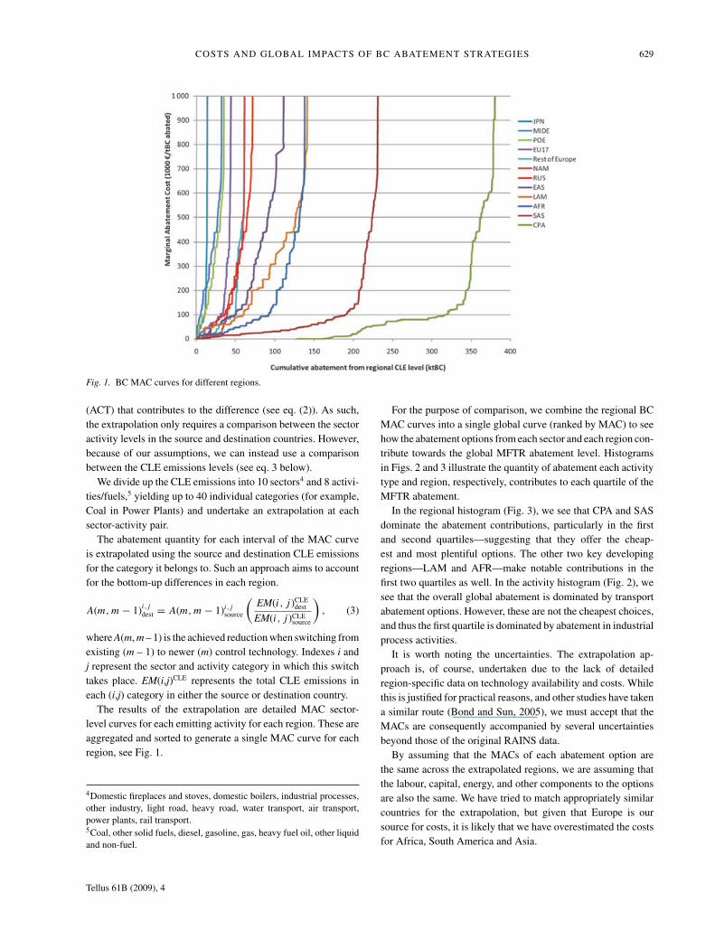
Fig. 1. BC MAC curves for different regions.

(ACT) that contributes to the difference (see eq. (2)). As such,the extrapolation only requires a comparison between the sectoractivity levels in the source and destination countries. However,because of our assumptions, we can instead use a comparisonbetween the CLE emissions levels (see eq. 3 below).

We divide up the CLE emissions into 10 sectors4 and 8 activi-ties/fuels,5 yielding up to 40 individual categories (for example,Coal in Power Plants) and undertake an extrapolation at eachsector-activity pair.

The abatement quantity for each interval of the MAC curveis extrapolated using the source and destination CLE emissionsfor the category it belongs to. Such an approach aims to accountfor the bottom-up differences in each region.

A(m, m − 1)i,jdest = A(m, m − 1)i,jsource

(EM(i, j )CLE

dest

EM(i, j )CLEsource

), (3)

where A(m, m – 1) is the achieved reduction when switching fromexisting (m – 1) to newer (m) control technology. Indexes i andj represent the sector and activity category in which this switchtakes place. EM(i,j)CLE represents the total CLE emissions ineach (i,j) category in either the source or destination country.

The results of the extrapolation are detailed MAC sector-level curves for each emitting activity for each region. These areaggregated and sorted to generate a single MAC curve for eachregion, see Fig. 1.

4Domestic fireplaces and stoves, domestic boilers, industrial processes,other industry, light road, heavy road, water transport, air transport,power plants, rail transport.5Coal, other solid fuels, diesel, gasoline, gas, heavy fuel oil, other liquidand non-fuel.

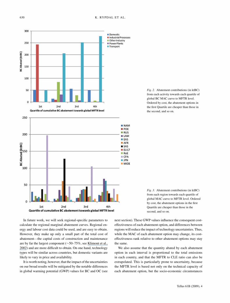
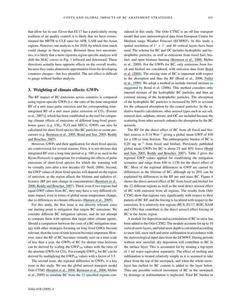
For the purpose of comparison, we combine the regional BCMAC curves into a single global curve (ranked by MAC) to seehow the abatement options from each sector and each region con-tribute towards the global MFTR abatement level. Histogramsin Figs. 2 and 3 illustrate the quantity of abatement each activitytype and region, respectively, contributes to each quartile of theMFTR abatement.

In the regional histogram (Fig. 3), we see that CPA and SASdominate the abatement contributions, particularly in the firstand second quartiles—suggesting that they offer the cheap-est and most plentiful options. The other two key developingregions—LAM and AFR—make notable contributions in thefirst two quartiles as well. In the activity histogram (Fig. 2), wesee that the overall global abatement is dominated by transportabatement options. However, these are not the cheapest choices,and thus the first quartile is dominated by abatement in industrialprocess activities.

It is worth noting the uncertainties. The extrapolation ap-proach is, of course, undertaken due to the lack of detailedregion-specific data on technology availability and costs. Whilethis is justified for practical reasons, and other studies have takena similar route (Bond and Sun, 2005), we must accept that theMACs are consequently accompanied by several uncertaintiesbeyond those of the original RAINS data.

By assuming that the MACs of each abatement option arethe same across the extrapolated regions, we are assuming thatthe labour, capital, energy, and other components to the optionsare also the same. We have tried to match appropriately similarcountries for the extrapolation, but given that Europe is oursource for costs, it is likely that we have overestimated the costsfor Africa, South America and Asia.

Tellus 61B (2009), 4

630 K. RYPDAL ET AL.

Fig. 2. Abatement contributions (in ktBC)from each activity towards each quartile ofglobal BC MAC curve to MFTR level.Ordered by cost, the abatement options inthe first Quartile are cheaper than those inthe second, and so on.

Fig. 3. Abatement contributions (in ktBC)from each region towards each quartile ofglobal MAC curve to MFTR level. Orderedby cost, the abatement options in the firstQuartile are cheaper than those in thesecond, and so on.

In future work, we will seek regional-specific parameters tocalculate the regional marginal abatement curves. Regional en-ergy and labour cost data could be used, and are easy to obtain.However, they make up only a small part of the total cost ofabatement—the capital costs of construction and maintenanceare by far the largest component (∼50–75%, see Klimont et al.,2002) and are more difficult to obtain. On one hand, technologytypes will be similar across countries, but domestic variants arelikely to vary in price and availability.

It is worth noting, however, that the impact of the uncertaintieson our broad results will be mitigated by the notable differencesin global warming potential (GWP) values for BC and OC (see

next section). These GWP values influence the consequent cost-effectiveness of each abatement option, and differences betweenregions will reduce the impact of technology uncertainties. Thus,while the MAC of each abatement option may change, its cost-effectiveness rank relative to other abatement options may staythe same.

We also assume that the quantity abated by each abatementoption in each interval is proportional to the total emissionsin each country, and that the MFTR to CLE ratio can also beextrapolated. This is particularly prone to uncertainty, becausethe MFTR level is based not only on the technical capacity ofeach abatement option, but the socio-economic circumstances

Tellus 61B (2009), 4

COSTS AND GLOBAL IMPACTS OF BC ABATEMENT STRATEGIES 631

that allow for its use. Given that EU17 has a particularly strongtradition of air quality control, it is likely that we have overes-timated the MFTR to CLE ratio for AFR, LAM and the Asianregions. However, our analysis is for 2030, by which time muchcould change in these regions. Between these two uncertain-ties, it is likely that a more rigorous region-specific analysis willshift the MAC curves in Fig. 1 leftward and downward. Thesedirections actually have opposite effects on the overall results,because they make abatement opportunities from the developingcountries cheaper—but less plentiful. The net effect is difficultto gauge without further analysis.

3. Weighting of climate effects: GWPs

The RF impact of BC emissions across countries is comparedusing region-specific GWPs [i.e. the ratio of the time-integratedRF of a unit mass pulse emission and the corresponding time-integrated RF of a unit mass pulse emission of CO2 (Forsteret al., 2007)], which has been established as the tool for compar-ing climate effects of emissions of different long-lived green-house gases (e.g. CH4, N2O and HFCs). GWPs can also becalculated for short-lived species like BC particles or ozone pre-cursors (e.g. Berntsen et al., 2005; Bond and Sun, 2005; Reddyand Boucher, 2007).

However, GWPs and their application for short-lived speciesare controversial for several reasons. First, it is not obvious thatintegrated RF over a long time period (e.g. 100 yr as used in theKyoto Protocol) is appropriate for evaluating the effects of pulseemissions of short-lived species for which the warming willbe virtually zero after a few decades (O’ Neill, 2000). Second,the GWP values of short-lived species will depend on the regionof emission, as the region affects the lifetime and radiative ef-ficiency (RF per unit change in concentration) (Berntsen et al.,2006; Reddy and Boucher, 2007). Third, even if two regions hadequal GWP values from BC, they may have a very different cli-mate impact, even in terms of global mean temperature change,due to differences in climate efficacies (Hansen et al., 2005).

For this study, the first issue is not directly relevant sinceour starting point is mitigation that targets BC emissions: Weconsider different BC mitigation options, and do not attemptto compare them with options that target other climate agents.Should a comparison between the costs of a BC mitigation strat-egy with other strategies focusing on long-lived GHGs becomerelevant, then the issue of time horizon becomes important. How-ever, since the RF of BC becomes virtually zero on a time scaleof less than a year, the GWPs of BC for shorter time horizonscan be derived by scaling the GWP100 values with the ratio ofthe absolute GWPs for CO2. For example GWP20 for BC can bederived by multiplying the GWP100 values with a factor of 3.5.

The second issue, the regional difference in GWPs, is a keyissue in this study. We use the global aerosol transport modelOslo CTM2 (Berglen et al., 2004; Berntsen et al., 2006; Myhreet al., 2009) to simulate BC from the 12 specified regions con-

sidered in this study. The Oslo CTM2 is an off-line transportmodel that uses meteorological data from European Centre forMedium range Weather Forecast (ECMWF). In this study aspatial resolution of 1◦ × 1◦ and 40 vertical layers have beenused. The scheme for BC and OC includes hydrophilic and hy-drophobic particles, as well as emissions from fossil fuel, bio-fuel, and open biomass burning (Berntsen et al., 2006; Myhreet al., 2009). For the GWPs for BC, only emissions from fos-sil and biofuel are considered, with emission data from Bondet al. (2004). The mixing state of BC is important with respectto the absorption and thus the RF (Bond et al., 2006; Fulleret al., 1999). We adopt a method to include internal mixture assuggested by Bond et al. (2006). This method considers onlyinternal mixture of the hydrophilic BC particles and thus anexternal mixing of the hydrophobic particles. The absorptionof the hydrophilic BC particles is increased by 50% to accountfor the enhanced absorption by the coated particles. In the ra-diative transfer calculations, other aerosol types such as sea salt,mineral dust, sulphate, nitrate, and OC are included because thescattering from other aerosols enhance the absorption by the BCaerosols.

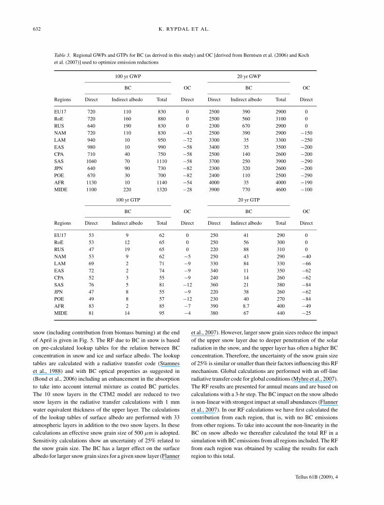
The RF for the direct effect of BC from all fossil and bio-fuel sources is 0.34 Wm−2 giving a global mean GWP of 830for a 100-yr time horizon. The anthropogenic burden of BC is0.20 mg m−2 from fossil and biofuel. Previously publishedglobal mean GWPs for BC is about 25 and 40% lower (Bondand Sun, 2005; Reddy and Boucher, 2007). Table 3 gives theregional GWP values applied for establishing the mitigationscenarios and range from 640 to 1130 for the direct effect ofBC. Most of the regional differences in GWP are caused bydifferences in the lifetime of BC, although up to 20% can beexplained by differences in the RF per unit mass BC. Figure 4shows the direct aerosol effect of BC from fossil and biofuel forthe 12 different regions as well as the total direct aerosol effectof BC with emission from all regions. The results from OsloCTM2 show that regions vary significantly with respect to theirpattern of BC RF, and the forcing is localized with respect to theemissions. It is relatively few regions (RUS, EU17, ROE, NAMand CPA) that contribute to the direct aerosol effect forcing ofBC in the Arctic region.

A module for deposition and accumulation of BC in snow hasbeen added to the Oslo CTM2. The module accounts for up to 10vertical snow layers, and total snow depth is calculated accordingto snow fall, snow melt and snow sublimation in accordance withthe meteorological input data from the ECMWF. During periodswithout new snowfall, dry deposition will contribute to BC inthe surface layer. This is accounted for by treating a top-layerof 1 ml water equivalent separately. The effect of melting andsublimation is treated relatively simple as it is assumed to takeplace from the top of the snowpack, and when the whole snow-layer has melted its BC content is added to the layer below.Thus any possible vertical movement of BC in the snowpackby drainage or sedimentation is neglected. Total BC burden in

Tellus 61B (2009), 4

632 K. RYPDAL ET AL.

Table 3. Regional GWPs and GTPs for BC (as derived in this study) and OC [derived from Berntsen et al. (2006) and Kochet al. (2007)] used to optimize emission reductions

100 yr GWP 20 yr GWP

BC OC BC OC

Regions Direct Indirect albedo Total Direct Direct Indirect albedo Total Direct

EU17 720 110 830 0 2500 390 2900 0RoE 720 160 880 0 2500 560 3100 0RUS 640 190 830 0 2300 670 2900 0NAM 720 110 830 −43 2500 390 2900 −150LAM 940 10 950 −72 3300 35 3300 −250EAS 980 10 990 −58 3400 35 3500 −200CPA 710 40 750 −58 2500 140 2600 −200SAS 1040 70 1110 −58 3700 250 3900 −290JPN 640 90 730 −82 2300 320 2600 −200POE 670 30 700 −82 2400 110 2500 −290AFR 1130 10 1140 −54 4000 35 4000 −190MIDE 1100 220 1320 −28 3900 770 4600 −100

100 yr GTP 20 yr GTP

BC OC BC OC

Regions Direct Indirect albedo Total Direct Direct Indirect albedo Total Direct

EU17 53 9 62 0 250 41 290 0RoE 53 12 65 0 250 56 300 0RUS 47 19 65 0 220 88 310 0NAM 53 9 62 −5 250 43 290 −40LAM 69 2 71 −9 330 84 330 −66EAS 72 2 74 −9 340 11 350 −62CPA 52 3 55 −9 240 14 260 −62SAS 76 5 81 −12 360 21 380 −84JPN 47 8 55 −9 220 38 260 −62POE 49 8 57 −12 230 40 270 −84AFR 83 2 85 −7 390 8.7 400 −49MIDE 81 14 95 −4 380 67 440 −25

snow (including contribution from biomass burning) at the endof April is given in Fig. 5. The RF due to BC in snow is basedon pre-calculated lookup tables for the relation between BCconcentration in snow and ice and surface albedo. The lookuptables are calculated with a radiative transfer code (Stamneset al., 1988) and with BC optical properties as suggested in(Bond et al., 2006) including an enhancement in the absorptionto take into account internal mixture as coated BC particles.The 10 snow layers in the CTM2 model are reduced to twosnow layers in the radiative transfer calculations with 1 mmwater equivalent thickness of the upper layer. The calculationsof the lookup tables of surface albedo are performed with 33atmospheric layers in addition to the two snow layers. In thesecalculations an effective snow grain size of 500 μm is adopted.Sensitivity calculations show an uncertainty of 25% related tothe snow grain size. The BC has a larger effect on the surfacealbedo for larger snow grain sizes for a given snow layer (Flanner

et al., 2007). However, larger snow grain sizes reduce the impactof the upper snow layer due to deeper penetration of the solarradiation in the snow, and the upper layer has often a higher BCconcentration. Therefore, the uncertainty of the snow grain sizeof 25% is similar or smaller than their factors influencing this RFmechanism. Global calculations are performed with an off-lineradiative transfer code for global conditions (Myhre et al., 2007).The RF results are presented for annual means and are based oncalculations with a 3-hr step. The BC impact on the snow albedois non-linear with strongest impact at small abundances (Flanneret al., 2007). In our RF calculations we have first calculated thecontribution from each region, that is, with no BC emissionsfrom other regions. To take into account the non-linearity in theBC on snow albedo we thereafter calculated the total RF in asimulation with BC emissions from all regions included. The RFfrom each region was obtained by scaling the results for eachregion to this total.

Tellus 61B (2009), 4

COSTS AND GLOBAL IMPACTS OF BC ABATEMENT STRATEGIES 633

Fig. 4. Radiative forcing of the direct aerosol effect of BC from fossil and biofuel of emissions from: (a) NAM; (b) POE; (c) RUS; (d) LAM; (e)EAS; (f) AFR; (g) SAS; (h) EU17; (i) RoE; (j) CPA; (k) JPN; (l) MIDE; (m) all regions.

The global and annual mean RF due to reduced surface albedocaused by BC in snow is calculated to be 0.03 Wm−2. Our explicitRF calculation is weaker than Reddy and Boucher (2007) andHansen and Nazarenko (2004). In Reddy and Boucher (2007)the RF of the BC impact on snow and ice albedo is specified to0.1 Wm−2 based on existing literature. Hansen and Nazarenko(2004) specified surface albedo changes of snow and ice, with

larger changes than our model results and a resulting RF thatis stronger. We have also a somewhat weaker RF (30%) thanFlanner et al. (2007) with an approach that is rather similar tothis study, but with different BC transport models and radiativetransfer schemes.

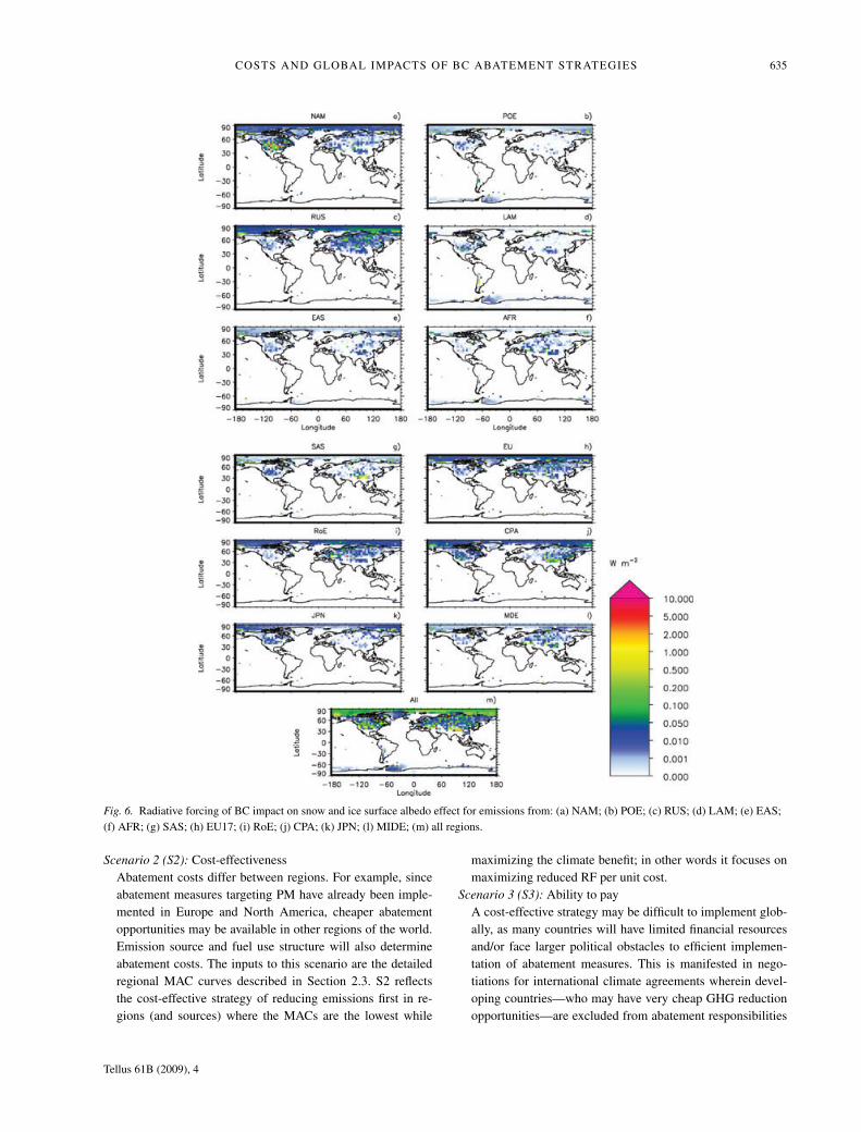
Figure 6 shows the RF due to BC impact on snow and icealbedo for emissions for selected regions. The physical-based

Tellus 61B (2009), 4

634 K. RYPDAL ET AL.

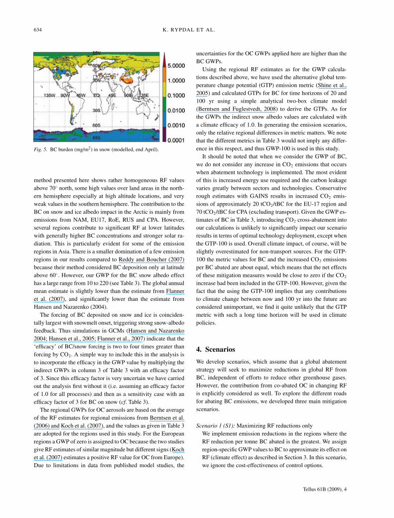
Fig. 5. BC burden (mg/m2) in snow (modelled, end April).

method presented here shows rather homogeneous RF valuesabove 70◦ north, some high values over land areas in the north-ern hemisphere especially at high altitude locations, and veryweak values in the southern hemisphere. The contribution to theBC on snow and ice albedo impact in the Arctic is mainly fromemissions from NAM, EU17, RoE, RUS and CPA. However,several regions contribute to significant RF at lower latitudeswith generally higher BC concentrations and stronger solar ra-diation. This is particularly evident for some of the emissionregions in Asia. There is a smaller domination of a few emissionregions in our results compared to Reddy and Boucher (2007)because their method considered BC deposition only at latitudeabove 60◦. However, our GWP for the BC snow albedo effecthas a large range from 10 to 220 (see Table 3). The global annualmean estimate is slightly lower than the estimate from Flanneret al. (2007), and significantly lower than the estimate fromHansen and Nazarenko (2004).

The forcing of BC deposited on snow and ice is coinciden-tally largest with snowmelt onset, triggering strong snow-albedofeedback. Thus simulations in GCMs (Hansen and Nazarenko2004; Hansen et al., 2005; Flanner et al., 2007) indicate that the‘efficacy’ of BC/snow forcing is two to four times greater thanforcing by CO2. A simple way to include this in the analysis isto incorporate the efficacy in the GWP value by multiplying theindirect GWPs in column 3 of Table 3 with an efficacy factorof 3. Since this efficacy factor is very uncertain we have carriedout the analysis first without it (i.e. assuming an efficacy factorof 1.0 for all processes) and then as a sensitivity case with anefficacy factor of 3 for BC on snow (cf. Table 3).

The regional GWPs for OC aerosols are based on the averageof the RF estimates for regional emissions from Berntsen et al.(2006) and Koch et al. (2007), and the values as given in Table 3are adopted for the regions used in this study. For the Europeanregions a GWP of zero is assigned to OC because the two studiesgive RF estimates of similar magnitude but different signs (Kochet al. (2007) estimates a positive RF value for OC from Europe).Due to limitations in data from published model studies, the

uncertainties for the OC GWPs applied here are higher than theBC GWPs.

Using the regional RF estimates as for the GWP calcula-tions described above, we have used the alternative global tem-perature change potential (GTP) emission metric (Shine et al.,2005) and calculated GTPs for BC for time horizons of 20 and100 yr using a simple analytical two-box climate model(Berntsen and Fuglestvedt, 2008) to derive the GTPs. As forthe GWPs the indirect snow albedo values are calculated witha climate efficacy of 1.0. In generating the emission scenarios,only the relative regional differences in metric matters. We notethat the different metrics in Table 3 would not imply any differ-ence in this respect, and thus GWP-100 is used in this study.

It should be noted that when we consider the GWP of BC,we do not consider any increase in CO2 emissions that occurswhen abatement technology is implemented. The most evidentof this is increased energy use required and the carbon leakagevaries greatly between sectors and technologies. Conservativerough estimates with GAINS results in increased CO2 emis-sions of approximately 20 tCO2/tBC for the EU-17 region and70 tCO2/tBC for CPA (excluding transport). Given the GWP es-timates of BC in Table 3, introducing CO2 cross-abatement intoour calculations is unlikely to significantly impact our scenarioresults in terms of optimal technology deployment, except whenthe GTP-100 is used. Overall climate impact, of course, will beslightly overestimated for non-transport sources. For the GTP-100 the metric values for BC and the increased CO2 emissionsper BC abated are about equal, which means that the net effectsof these mitigation measures would be close to zero if the CO2

increase had been included in the GTP-100. However, given thefact that the using the GTP-100 implies that any contributionsto climate change between now and 100 yr into the future areconsidered unimportant, we find it quite unlikely that the GTPmetric with such a long time horizon will be used in climatepolicies.

4. Scenarios

We develop scenarios, which assume that a global abatementstrategy will seek to maximize reductions in global RF fromBC, independent of efforts to reduce other greenhouse gases.However, the contribution from co-abated OC in changing RFis explicitly considered as well. To explore the different roadsfor abating BC emissions, we developed three main mitigationscenarios.

Scenario 1 (S1): Maximizing RF reductions onlyWe implement emission reductions in the regions where theRF reduction per tonne BC abated is the greatest. We assignregion-specific GWP values to BC to approximate its effect onRF (climate effect) as described in Section 3. In this scenario,we ignore the cost-effectiveness of control options.

Tellus 61B (2009), 4

COSTS AND GLOBAL IMPACTS OF BC ABATEMENT STRATEGIES 635

Fig. 6. Radiative forcing of BC impact on snow and ice surface albedo effect for emissions from: (a) NAM; (b) POE; (c) RUS; (d) LAM; (e) EAS;(f) AFR; (g) SAS; (h) EU17; (i) RoE; (j) CPA; (k) JPN; (l) MIDE; (m) all regions.

Scenario 2 (S2): Cost-effectivenessAbatement costs differ between regions. For example, sinceabatement measures targeting PM have already been imple-mented in Europe and North America, cheaper abatementopportunities may be available in other regions of the world.Emission source and fuel use structure will also determineabatement costs. The inputs to this scenario are the detailedregional MAC curves described in Section 2.3. S2 reflectsthe cost-effective strategy of reducing emissions first in re-gions (and sources) where the MACs are the lowest while

maximizing the climate benefit; in other words it focuses onmaximizing reduced RF per unit cost.

Scenario 3 (S3): Ability to payA cost-effective strategy may be difficult to implement glob-ally, as many countries will have limited financial resourcesand/or face larger political obstacles to efficient implemen-tation of abatement measures. This is manifested in nego-tiations for international climate agreements wherein devel-oping countries—who may have very cheap GHG reductionopportunities—are excluded from abatement responsibilities

Tellus 61B (2009), 4

636 K. RYPDAL ET AL.

on the grounds of their ability to pay: ‘common but differ-entiated responsibilities’. We use the gross domestic prod-uct (GDP) per capita as a proxy for the ability to pay [asused by e.g. Dinwiddy and Teal (1996)], scaling regionalabatement costs linearly by relative GDP per capita. In S3,we thus maximize reduced RF per unit abated weightedby relative GDP per capita. Regional GDP per capita for2030 was taken from the downscaled SRES database athttp://www.ciesin.columbia.edu/datasets/downscaled/.

Finally, we considered each scenario under three differenttargets: reducing the global BC RF by 10, 20 and 30%, respec-tively, hereafter named ‘RF-10’, ‘RF-20’ and ‘RF-30’. We runthree versions of all scenarios with respect to the climate ef-fect: one that takes into account the direct climate effect only, asecond that also takes into account the indirect effect of BC de-posited on snow and a third that considers the enhanced climateefficacy of BC deposited on snow. Thus, altogether 27 differentruns have been made. The absolute value of the forcing doesnot matter in the optimizations, but the consideration of BC de-posited on snow implies different regional weights compared toconsidering the direct effect only. The semi-direct effect is notincluded in the analysis, as even the global estimates for this arevery uncertain.

5. Results

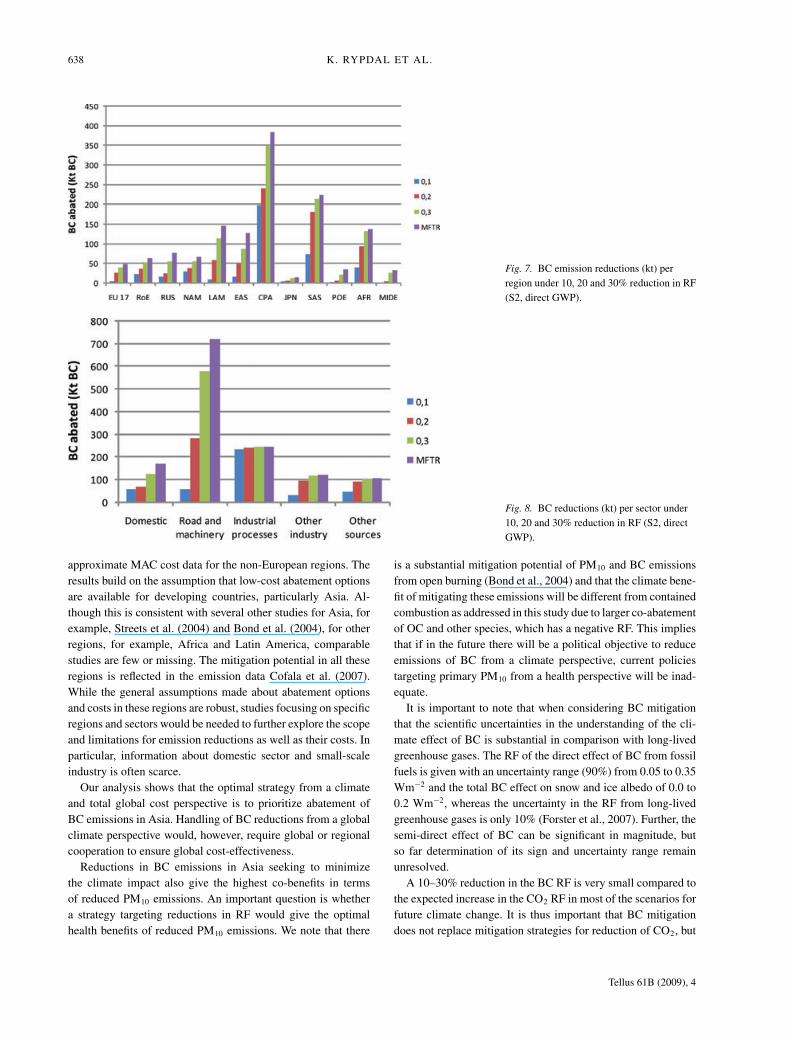
The resulting emission reductions are shown in Table 4 for totalemissions and in Table 5 and Fig. 7 for regional emissions.Applying all the emission control measures available in themodel (MTFR scenario) achieves globally 35% reduction ofBC RF.

In S1, mitigation takes place first in the regions with thehighest GWP. Taking into account the direct GWP only, the most

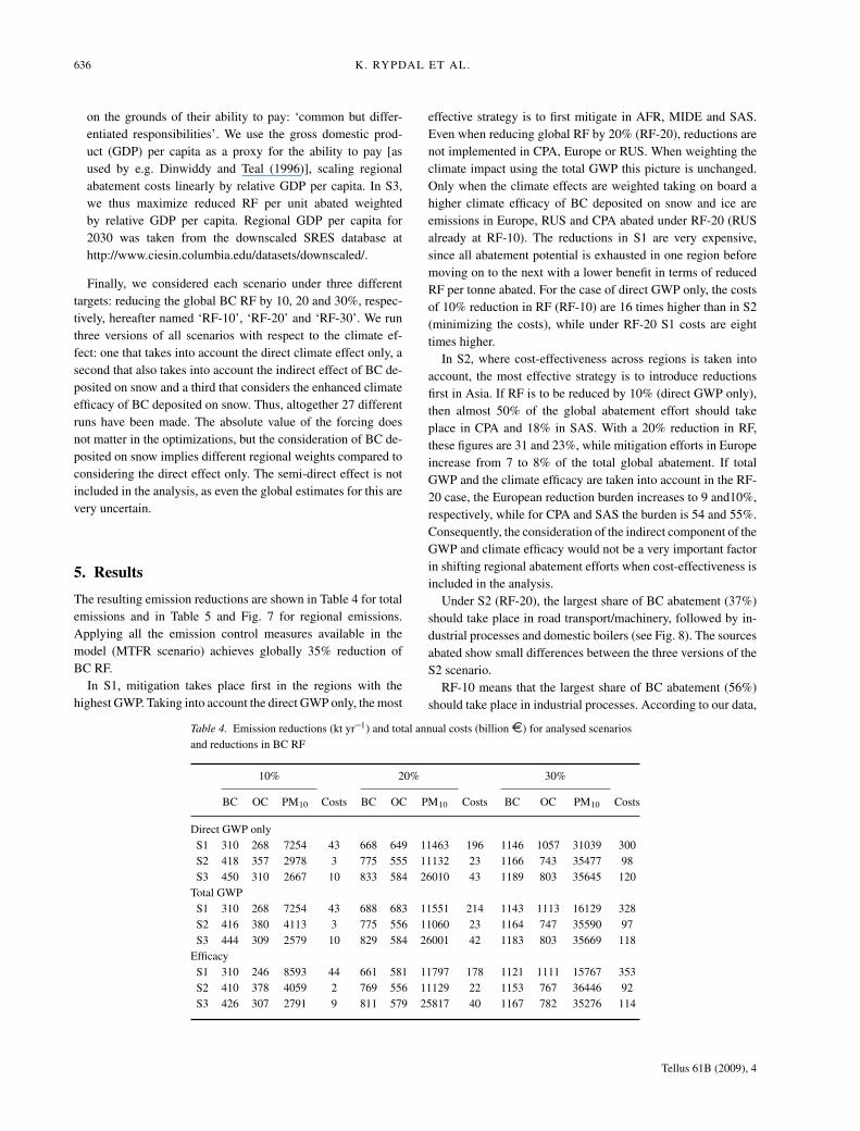
Table 4. Emission reductions (kt yr–1) and total annual costs (billion €) for analysed scenariosand reductions in BC RF

10% 20% 30%

BC OC PM10 Costs BC OC PM10 Costs BC OC PM10 Costs

Direct GWP onlyS1 310 268 7254 43 668 649 11463 196 1146 1057 31039 300S2 418 357 2978 3 775 555 11132 23 1166 743 35477 98S3 450 310 2667 10 833 584 26010 43 1189 803 35645 120

Total GWPS1 310 268 7254 43 688 683 11551 214 1143 1113 16129 328S2 416 380 4113 3 775 556 11060 23 1164 747 35590 97S3 444 309 2579 10 829 584 26001 42 1183 803 35669 118

EfficacyS1 310 246 8593 44 661 581 11797 178 1121 1111 15767 353S2 410 378 4059 2 769 556 11129 22 1153 767 36446 92S3 426 307 2791 9 811 579 25817 40 1167 782 35276 114

effective strategy is to first mitigate in AFR, MIDE and SAS.Even when reducing global RF by 20% (RF-20), reductions arenot implemented in CPA, Europe or RUS. When weighting theclimate impact using the total GWP this picture is unchanged.Only when the climate effects are weighted taking on board ahigher climate efficacy of BC deposited on snow and ice areemissions in Europe, RUS and CPA abated under RF-20 (RUSalready at RF-10). The reductions in S1 are very expensive,since all abatement potential is exhausted in one region beforemoving on to the next with a lower benefit in terms of reducedRF per tonne abated. For the case of direct GWP only, the costsof 10% reduction in RF (RF-10) are 16 times higher than in S2(minimizing the costs), while under RF-20 S1 costs are eighttimes higher.

In S2, where cost-effectiveness across regions is taken intoaccount, the most effective strategy is to introduce reductionsfirst in Asia. If RF is to be reduced by 10% (direct GWP only),then almost 50% of the global abatement effort should takeplace in CPA and 18% in SAS. With a 20% reduction in RF,these figures are 31 and 23%, while mitigation efforts in Europeincrease from 7 to 8% of the total global abatement. If totalGWP and the climate efficacy are taken into account in the RF-20 case, the European reduction burden increases to 9 and10%,respectively, while for CPA and SAS the burden is 54 and 55%.Consequently, the consideration of the indirect component of theGWP and climate efficacy would not be a very important factorin shifting regional abatement efforts when cost-effectiveness isincluded in the analysis.

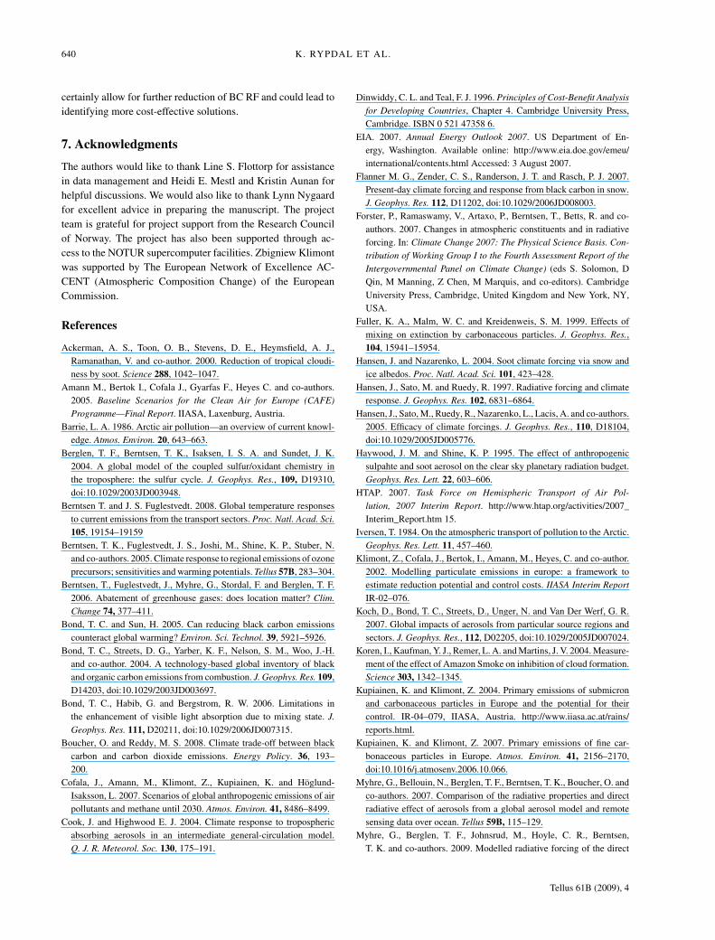
Under S2 (RF-20), the largest share of BC abatement (37%)should take place in road transport/machinery, followed by in-dustrial processes and domestic boilers (see Fig. 8). The sourcesabated show small differences between the three versions of theS2 scenario.

RF-10 means that the largest share of BC abatement (56%)should take place in industrial processes. According to our data,

Tellus 61B (2009), 4

COSTS AND GLOBAL IMPACTS OF BC ABATEMENT STRATEGIES 637

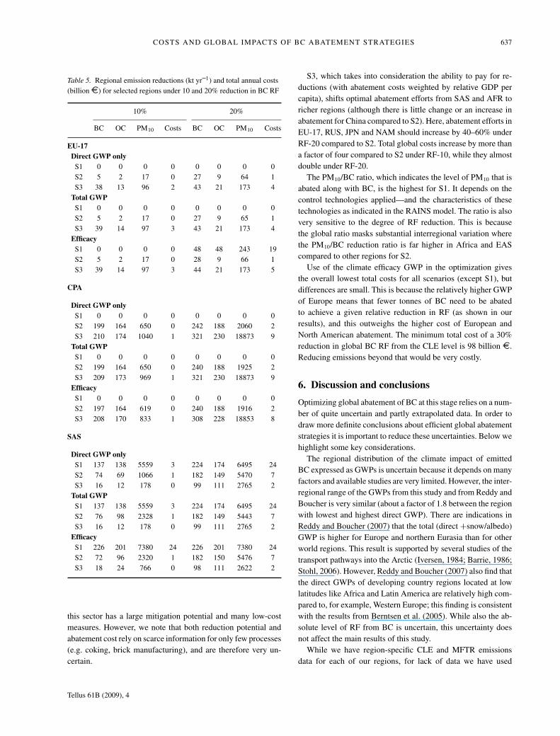
Table 5. Regional emission reductions (kt yr–1) and total annual costs(billion €) for selected regions under 10 and 20% reduction in BC RF

10% 20%

BC OC PM10 Costs BC OC PM10 Costs

EU-17Direct GWP only

S1 0 0 0 0 0 0 0 0S2 5 2 17 0 27 9 64 1S3 38 13 96 2 43 21 173 4

Total GWPS1 0 0 0 0 0 0 0 0S2 5 2 17 0 27 9 65 1S3 39 14 97 3 43 21 173 4

EfficacyS1 0 0 0 0 48 48 243 19S2 5 2 17 0 28 9 66 1S3 39 14 97 3 44 21 173 5

CPA

Direct GWP onlyS1 0 0 0 0 0 0 0 0S2 199 164 650 0 242 188 2060 2S3 210 174 1040 1 321 230 18873 9

Total GWPS1 0 0 0 0 0 0 0 0S2 199 164 650 0 240 188 1925 2S3 209 173 969 1 321 230 18873 9

EfficacyS1 0 0 0 0 0 0 0 0S2 197 164 619 0 240 188 1916 2S3 208 170 833 1 308 228 18853 8

SAS

Direct GWP onlyS1 137 138 5559 3 224 174 6495 24S2 74 69 1066 1 182 149 5470 7S3 16 12 178 0 99 111 2765 2

Total GWPS1 137 138 5559 3 224 174 6495 24S2 76 98 2328 1 182 149 5443 7S3 16 12 178 0 99 111 2765 2

EfficacyS1 226 201 7380 24 226 201 7380 24S2 72 96 2320 1 182 150 5476 7S3 18 24 766 0 98 111 2622 2

this sector has a large mitigation potential and many low-costmeasures. However, we note that both reduction potential andabatement cost rely on scarce information for only few processes(e.g. coking, brick manufacturing), and are therefore very un-certain.

S3, which takes into consideration the ability to pay for re-ductions (with abatement costs weighted by relative GDP percapita), shifts optimal abatement efforts from SAS and AFR toricher regions (although there is little change or an increase inabatement for China compared to S2). Here, abatement efforts inEU-17, RUS, JPN and NAM should increase by 40–60% underRF-20 compared to S2. Total global costs increase by more thana factor of four compared to S2 under RF-10, while they almostdouble under RF-20.

The PM10/BC ratio, which indicates the level of PM10 that isabated along with BC, is the highest for S1. It depends on thecontrol technologies applied—and the characteristics of thesetechnologies as indicated in the RAINS model. The ratio is alsovery sensitive to the degree of RF reduction. This is becausethe global ratio masks substantial interregional variation wherethe PM10/BC reduction ratio is far higher in Africa and EAScompared to other regions for S2.

Use of the climate efficacy GWP in the optimization givesthe overall lowest total costs for all scenarios (except S1), butdifferences are small. This is because the relatively higher GWPof Europe means that fewer tonnes of BC need to be abatedto achieve a given relative reduction in RF (as shown in ourresults), and this outweighs the higher cost of European andNorth American abatement. The minimum total cost of a 30%reduction in global BC RF from the CLE level is 98 billion €.Reducing emissions beyond that would be very costly.

6. Discussion and conclusions

Optimizing global abatement of BC at this stage relies on a num-ber of quite uncertain and partly extrapolated data. In order todraw more definite conclusions about efficient global abatementstrategies it is important to reduce these uncertainties. Below wehighlight some key considerations.

The regional distribution of the climate impact of emittedBC expressed as GWPs is uncertain because it depends on manyfactors and available studies are very limited. However, the inter-regional range of the GWPs from this study and from Reddy andBoucher is very similar (about a factor of 1.8 between the regionwith lowest and highest direct GWP). There are indications inReddy and Boucher (2007) that the total (direct +snow/albedo)GWP is higher for Europe and northern Eurasia than for otherworld regions. This result is supported by several studies of thetransport pathways into the Arctic (Iversen, 1984; Barrie, 1986;Stohl, 2006). However, Reddy and Boucher (2007) also find thatthe direct GWPs of developing country regions located at lowlatitudes like Africa and Latin America are relatively high com-pared to, for example, Western Europe; this finding is consistentwith the results from Berntsen et al. (2005). While also the ab-solute level of RF from BC is uncertain, this uncertainty doesnot affect the main results of this study.

While we have region-specific CLE and MFTR emissionsdata for each of our regions, for lack of data we have used

Tellus 61B (2009), 4

638 K. RYPDAL ET AL.

Fig. 7. BC emission reductions (kt) perregion under 10, 20 and 30% reduction in RF(S2, direct GWP).

Fig. 8. BC reductions (kt) per sector under10, 20 and 30% reduction in RF (S2, directGWP).

approximate MAC cost data for the non-European regions. Theresults build on the assumption that low-cost abatement optionsare available for developing countries, particularly Asia. Al-though this is consistent with several other studies for Asia, forexample, Streets et al. (2004) and Bond et al. (2004), for otherregions, for example, Africa and Latin America, comparablestudies are few or missing. The mitigation potential in all theseregions is reflected in the emission data Cofala et al. (2007).While the general assumptions made about abatement optionsand costs in these regions are robust, studies focusing on specificregions and sectors would be needed to further explore the scopeand limitations for emission reductions as well as their costs. Inparticular, information about domestic sector and small-scaleindustry is often scarce.

Our analysis shows that the optimal strategy from a climateand total global cost perspective is to prioritize abatement ofBC emissions in Asia. Handling of BC reductions from a globalclimate perspective would, however, require global or regionalcooperation to ensure global cost-effectiveness.

Reductions in BC emissions in Asia seeking to minimizethe climate impact also give the highest co-benefits in termsof reduced PM10 emissions. An important question is whethera strategy targeting reductions in RF would give the optimalhealth benefits of reduced PM10 emissions. We note that there

is a substantial mitigation potential of PM10 and BC emissionsfrom open burning (Bond et al., 2004) and that the climate bene-fit of mitigating these emissions will be different from containedcombustion as addressed in this study due to larger co-abatementof OC and other species, which has a negative RF. This impliesthat if in the future there will be a political objective to reduceemissions of BC from a climate perspective, current policiestargeting primary PM10 from a health perspective will be inad-equate.

It is important to note that when considering BC mitigationthat the scientific uncertainties in the understanding of the cli-mate effect of BC is substantial in comparison with long-livedgreenhouse gases. The RF of the direct effect of BC from fossilfuels is given with an uncertainty range (90%) from 0.05 to 0.35Wm−2 and the total BC effect on snow and ice albedo of 0.0 to0.2 Wm−2, whereas the uncertainty in the RF from long-livedgreenhouse gases is only 10% (Forster et al., 2007). Further, thesemi-direct effect of BC can be significant in magnitude, butso far determination of its sign and uncertainty range remainunresolved.

A 10–30% reduction in the BC RF is very small compared tothe expected increase in the CO2 RF in most of the scenarios forfuture climate change. It is thus important that BC mitigationdoes not replace mitigation strategies for reduction of CO2, but

Tellus 61B (2009), 4

COSTS AND GLOBAL IMPACTS OF BC ABATEMENT STRATEGIES 639

Table 6. Economically efficient global BC abatement (kt yr–1 BC) under alternativeprevailing CO2 permit prices and BC metric in scenario S2. OC co-abatement isaccounted for

Permit price in 2030 20 €/tCO2 30 €/tCO2 40 €/tCO2 60 €/tCO2

GWP-100 direct 378 459 502 586GWP-100 total 404 466 509 613GWP-100 efficacy 423 485 522 632GWP-20 direct 649 791 928 1008GWP-20 total 668 828 949 1022GWP-20 efficacy 707 898 966 1042GTP-100 total 266 266 266 288GTP-20 total 292 304 315 410

rather complement them. An important question is yet whetherthe climate impact and abatement costs of BC indicates that itis a cost-effective means of climate mitigation, as compared tothe prevailing prices of CO2 permits. This would provide jus-tification for reducing BC alongside other forcing agents suchas the six Kyoto Protocol gases. This depends on the value ofthe GWP relative to other forcing agents, which is very depen-dent on the time horizon considered and whether the indirecteffect and enhanced efficacy is taken into account. One way tolook at this is to assess how much global BC abatement is war-ranted under alternative prevailing CO2 permit prices. As high-lighted above, our BC abatement costs are in annualized format,and can thus be compared to equivalent CO2 abatement costs.Table 6 explores the economically efficient BC abatement levelsin scenario S2 for direct, total, and efficacy approaches to the100-yr GWP of BC. Given the projected global CLE BC levelsof approximately 5000 kt BC in 2030, the range of efficient BCabatement is between 8 and 12% for CO2 permit prices of 20–60€/tCO2. We see that even with a trebling of the permit price,the economical level of abatement only rises by 50%.

Of course, indirect effect and especially the efficacies of BCdeposited on snow provide a stronger justification for abatement.This is because the overall BC emission reduction is smaller toachieve 1 tonne equivalent CO2. On the other hand, the indirectcomponent at present is more uncertain than the direct, so therecan be larger obstacles to its use it in the design of BC policies.Considering a shorter time horizon than 100 years will of coursealso emphasize reductions in BC over other forcing agents. Thisis illustrated in Table 6 for 20 yr time-horizon. The 20 yr time-horizon will imply a range of efficient BC abatement between13 and 20% (65–87% higher mass of BC abated compared tousing GWP-100 as a metric).

Furthermore, since the GTPs do not include the strong short-term warming effect of BC immediately after the emissions,the GTPs are significantly lower than the GWPs, yielding lowerlevels of efficient abatement. Yet the efficient level is ratherinsensitive to the choice of metric (GWP-100 versus GTP-100).A decrease of the BC equivalent CO2 value by a factor of more

than 10 only decreases the efficient global BC abatement by 30%.Moreover, the ratio of efficient levels for across time horizons(20-/100-yr) is significantly different between the GWP andGTP metrics, and for GTP-100 there little sensitivity to the CO2

permit price in the range 20–40 €/ tCO2.These patterns and sensitivities of efficient abatement levels

can largely be explained by the shape of the MAC curve at theprevailing price of carbon. They are made up of flat sections andsteep cliffs, which respectively make the efficient levels highlysensitive or insensitive to choice of metric and time horizon(see Fig. 1). The economically efficient amount of abatementdepends on the point along the MAC curve upon which the€/t equivalent CO2-denominated carbon price lies. For a givencarbon price, this point is different depending on the choiceof metric and time-horizon. However, an initial plateau coversthe abatement to approximately 225 ktBC, which is well under€2/tCO2 equivalent for all the metrics and time-horizons wehave examined. Thus, over the, CO2 prices we have examined,the first 225 ktBC is always economically efficient.

Furthermore, the sensitivity of the efficient abatement level tochanges in the carbon price depends on the shape of the MACat the initial price point. For example, under the GWP metric,the MAC curve at €20/t equivalent CO2 is generally steep,meaning a move towards €60 yields only minor additions tothe efficient level. Under the GTP-100 metric, the MAC curverises almost vertically at €20/t equivalent CO2, so there is verylittle additional economical abatement as the carbon price risesto €60. Under GTP-20, however, the curve is comparably lesssteep at €20, allowing for a larger increase in efficient abatementwith higher prices.

Finally, we note that the overall mitigation potential estimatedfor 2030 derives from information about the performance of cur-rently commercialized technical measures to improve efficiencyand abate emissions. Surely, the future will bring new tech-nologies but a more important aspect is structural changes inthe energy system that would result in increased penetrationof clean fuels. Consequently, adding in the analysis potentialfor fuel switching and impacts of future technologies would

Tellus 61B (2009), 4

640 K. RYPDAL ET AL.

certainly allow for further reduction of BC RF and could lead toidentifying more cost-effective solutions.

7. Acknowledgments

The authors would like to thank Line S. Flottorp for assistancein data management and Heidi E. Mestl and Kristin Aunan forhelpful discussions. We would also like to thank Lynn Nygaardfor excellent advice in preparing the manuscript. The projectteam is grateful for project support from the Research Councilof Norway. The project has also been supported through ac-cess to the NOTUR supercomputer facilities. Zbigniew Klimontwas supported by The European Network of Excellence AC-CENT (Atmospheric Composition Change) of the EuropeanCommission.

References

Ackerman, A. S., Toon, O. B., Stevens, D. E., Heymsfield, A. J.,Ramanathan, V. and co-author. 2000. Reduction of tropical cloudi-ness by soot. Science 288, 1042–1047.

Amann M., Bertok I., Cofala J., Gyarfas F., Heyes C. and co-authors.2005. Baseline Scenarios for the Clean Air for Europe (CAFE)

Programme—Final Report. IIASA, Laxenburg, Austria.Barrie, L. A. 1986. Arctic air pollution—an overview of current knowl-

edge. Atmos. Environ. 20, 643–663.Berglen, T. F., Berntsen, T. K., Isaksen, I. S. A. and Sundet, J. K.

2004. A global model of the coupled sulfur/oxidant chemistry inthe troposphere: the sulfur cycle. J. Geophys. Res., 109, D19310,doi:10.1029/2003JD003948.

Berntsen T. and J. S. Fuglestvedt. 2008. Global temperature responsesto current emissions from the transport sectors. Proc. Natl. Acad. Sci.

105, 19154–19159Berntsen, T. K., Fuglestvedt, J. S., Joshi, M., Shine, K. P., Stuber, N.

and co-authors. 2005. Climate response to regional emissions of ozoneprecursors; sensitivities and warming potentials. Tellus 57B, 283–304.

Berntsen, T., Fuglestvedt, J., Myhre, G., Stordal, F. and Berglen, T. F.2006. Abatement of greenhouse gases: does location matter? Clim.

Change 74, 377–411.Bond, T. C. and Sun, H. 2005. Can reducing black carbon emissions

counteract global warming? Environ. Sci. Technol. 39, 5921–5926.Bond, T. C., Streets, D. G., Yarber, K. F., Nelson, S. M., Woo, J.-H.

and co-author. 2004. A technology-based global inventory of blackand organic carbon emissions from combustion. J. Geophys. Res. 109,D14203, doi:10.1029/2003JD003697.

Bond, T. C., Habib, G. and Bergstrom, R. W. 2006. Limitations inthe enhancement of visible light absorption due to mixing state. J.

Geophys. Res. 111, D20211, doi:10.1029/2006JD007315.Boucher, O. and Reddy, M. S. 2008. Climate trade-off between black

carbon and carbon dioxide emissions. Energy Policy. 36, 193–200.

Cofala, J., Amann, M., Klimont, Z., Kupiainen, K. and Hoglund-Isaksson, L. 2007. Scenarios of global anthropogenic emissions of airpollutants and methane until 2030. Atmos. Environ. 41, 8486–8499.

Cook, J. and Highwood E. J. 2004. Climate response to troposphericabsorbing aerosols in an intermediate general-circulation model.Q. J. R. Meteorol. Soc. 130, 175–191.

Dinwiddy, C. L. and Teal, F. J. 1996. Principles of Cost-Benefit Analysis

for Developing Countries, Chapter 4. Cambridge University Press,Cambridge. ISBN 0 521 47358 6.

EIA. 2007. Annual Energy Outlook 2007. US Department of En-ergy, Washington. Available online: http://www.eia.doe.gov/emeu/international/contents.html Accessed: 3 August 2007.

Flanner M. G., Zender, C. S., Randerson, J. T. and Rasch, P. J. 2007.Present-day climate forcing and response from black carbon in snow.J. Geophys. Res. 112, D11202, doi:10.1029/2006JD008003.

Forster, P., Ramaswamy, V., Artaxo, P., Berntsen, T., Betts, R. and co-authors. 2007. Changes in atmospheric constituents and in radiativeforcing. In: Climate Change 2007: The Physical Science Basis. Con-

tribution of Working Group I to the Fourth Assessment Report of the

Intergovernmental Panel on Climate Change) (eds S. Solomon, DQin, M Manning, Z Chen, M Marquis, and co-editors). CambridgeUniversity Press, Cambridge, United Kingdom and New York, NY,USA.

Fuller, K. A., Malm, W. C. and Kreidenweis, S. M. 1999. Effects ofmixing on extinction by carbonaceous particles. J. Geophys. Res.,104, 15941–15954.

Hansen, J. and Nazarenko, L. 2004. Soot climate forcing via snow andice albedos. Proc. Natl. Acad. Sci. 101, 423–428.

Hansen, J., Sato, M. and Ruedy, R. 1997. Radiative forcing and climateresponse. J. Geophys. Res. 102, 6831–6864.

Hansen, J., Sato, M., Ruedy, R., Nazarenko, L., Lacis, A. and co-authors.2005. Efficacy of climate forcings. J. Geophys. Res., 110, D18104,doi:10.1029/2005JD005776.

Haywood, J. M. and Shine, K. P. 1995. The effect of anthropogenicsulpahte and soot aerosol on the clear sky planetary radiation budget.Geophys. Res. Lett. 22, 603–606.

HTAP. 2007. Task Force on Hemispheric Transport of Air Pol-lution, 2007 Interim Report. http://www.htap.org/activities/2007_Interim_Report.htm 15.

Iversen, T. 1984. On the atmospheric transport of pollution to the Arctic.Geophys. Res. Lett. 11, 457–460.

Klimont, Z., Cofala, J., Bertok, I., Amann, M., Heyes, C. and co-author.2002. Modelling particulate emissions in europe: a framework toestimate reduction potential and control costs. IIASA Interim Report

IR-02–076.Koch, D., Bond, T. C., Streets, D., Unger, N. and Van Der Werf, G. R.

2007. Global impacts of aerosols from particular source regions andsectors. J. Geophys. Res., 112, D02205, doi:10.1029/2005JD007024.

Koren, I., Kaufman, Y. J., Remer, L. A. and Martins, J. V. 2004. Measure-ment of the effect of Amazon Smoke on inhibition of cloud formation.Science 303, 1342–1345.

Kupiainen, K. and Klimont, Z. 2004. Primary emissions of submicronand carbonaceous particles in Europe and the potential for theircontrol. IR-04–079, IIASA, Austria. http://www.iiasa.ac.at/rains/reports.html.

Kupiainen, K. and Klimont, Z. 2007. Primary emissions of fine car-bonaceous particles in Europe. Atmos. Environ. 41, 2156–2170,doi:10.1016/j.atmosenv.2006.10.066.

Myhre, G., Bellouin, N., Berglen, T. F., Berntsen, T. K., Boucher, O. andco-authors. 2007. Comparison of the radiative properties and directradiative effect of aerosols from a global aerosol model and remotesensing data over ocean. Tellus 59B, 115–129.

Myhre, G., Berglen, T. F., Johnsrud, M., Hoyle, C. R., Berntsen,T. K. and co-authors. 2009. Modelled radiative forcing of the direct

Tellus 61B (2009), 4

COSTS AND GLOBAL IMPACTS OF BC ABATEMENT STRATEGIES 641

aerosol effect with multi-observation evaluation. Atmos. Chem. Phys.,9, 1365–1392.

Naik, V., Mauzerall, D. L., Horrowitz, L.W, Schwarzkopf, M. D.,Ramaswamy, V. and co-author. 2007. On the sensitivity of radiativeforcing from biomass burning aerosols and ozone to emission loca-tion. Geophys. Res. Lett. 34, L03818, doi:10.1029/2006GL028149.

O‘Neill, B. C. 2000. The Jury is still out on global warming potentials.Clim. Change 44, 427–443.

Ramanathan, V. and Carmichael, G. 2008. Global and regional climatechanges due to black carbon. Nat. Geosci. 1, 221–227.

Ramaswamy, V., Boucher, O., Haigh, J., Hauglustaine, D., Haywood, J.and co-authors 2001. Radiative forcing of climate change. In: Climate

Change 2001: The Scientific Basis. Contribution of Working Group

I to the Third Assessment Report of the Intergovernmental Panel onClimate Change (eds. JT Houghton et al.). Cambridge UniversityPress, Cambridge, United Kingdom and New York, NY, USA, 349–416.

Reddy, M. S. and Boucher, O. 2007. Climate impact of black carbonemitted from energy consumption in the world’s regions. Geophys.

Res. Lett. 34, L11802, doi:10.1029/2006GL028904.Shine, K. P., Fuglestvedt, J. S., Hailemariam, K. and Stuber, N. 2005.

Alternatives to the global warming potential for comparing climate

impacts of emissions of greenhouse gases. Clim. Change 68, 281–302.

Schulz M., Textor, C., Kinne, S., Balkanski, Y., Bauer, S. and co-authors.2006. Radiative forcing by aerosols as derived from the AeroCompresent-day and pre-industrial simulations. Atmos. Chem. Phys. 6,5225–5246.

Stamnes, K., Tsay, S. C., Wiscombe, W. and Jayaweera, K. 1988. Numer-ically stable algorithm for discrete-ordinate-method radiative-transferin multiple-scattering and emitting layered media. Appl. Opt. 27,2502–2509.

Stohl, A. 2006. Characteristics of atmospheric transport intothe Arctic troposphere. J. Geophys. Res. 111, D11306,doi:10.1029/2005JD006888.

Streets, D. G., Bond, T. C., Lee. T. and Jang, C. 2004. On the futureof carbonaceous aerosol emissions. J. Geophys. Res., 109, D24212,doi:10.1029/2004JD004902.

Warren, S. G. 1984. Impurities in snow: effects on albedo and snowmelt.Ann. Glaciol. 5, 177–179.

WHO. 2004. Health Aspects of Air Pollution. Results from theWHO project “Systematic Review of Health Aspects of Air Pol-lution in Europe”. World Health Organization. http://ec.europa.eu/environment/air/cafe/activities/pdf/e83080.pdf.

Tellus 61B (2009), 4