A DEA based estimation on abatement cost savings

CEEP-BIT WORKING PAPER SERIES

Potential gains from carbon emissions trading in China: A DEA

based estimation on abatement cost savings

Ke Wang

Yi-Ming Wei

Zhimin Huang

Working Paper 84

http://ceep.bit.edu.cn/english/publications/wp/index.htm

Center for Energy and Environmental Policy Research

Beijing Institute of Technology

No.5 Zhongguancun South Street, Haidian District

Beijing 100081

January 2015

This paper can be cited as: Wang K, Wei Y-M, Huang Z. 2015. Potential gains from carbon

emissions trading in China: A DEA based estimation on abatement cost savings. CEEP-BIT

Working Paper.

The authors gratefully acknowledge the financial support from the National Natural Science

Foundation of China (grant nos. 71471018 and 71101011) and the Outstanding Young

Teachers Foundation of Beijing Institute of Technology (grant no. 2013YR2119). The views

expressed herein are those of the authors and do not necessarily reflect the views of the

Center for Energy and Environmental Policy Research.

© 2015 by Ke Wang, Yi-Ming Wei and Zhimin Huang. All rights reserved.

The Center for Energy and Environmental Policy Research, Beijing Institute of Technology

(CEEP-BIT), was established in 2009. CEEP-BIT conducts researches on energy economics,

climate policy and environmental management to provide scientific basis for public and

private decisions in strategy planning and management. CEEP-BIT serves as the platform for

the international exchange in the area of energy and environmental policy.

Currently, CEEP-BIT Ranks 47, top 3% institutions in the field of Energy Economics at

IDEAS（http://ideas.repec.org/top/top.ene.htm), and Ranks 52, top 3% institutions in the field

of Environmental Economics at IDEAS (http://ideas.repec.org/ top/top.env.html).

Yi-Ming Wei

Director of Center for Energy and Environmental Policy Research, Beijing Institute of

Technology

For more information, please contact the office:

Address:

Director of Center for Energy and Environmental Policy Research

Beijing Institute of Technology

No.5 Zhongguancun South Street

Haidian District, Beijing 100081, P.R. China

Access:

Tel: +86-10-6891-8551

Fax: +86-10-6891-8651

Email: [email protected]

Website: http://ceep.bit.edu.cn/english/index.htm

Potential gains from carbon emissions trading in China: A DEA based

estimation on abatement cost savings

Ke Wang a,b,c,1, Yi-Ming Wei a,b,c, Zhimin Huang a,b,d

a Center for Energy and Environmental Policy Research, Beijing Institute of Technology, Beijing, China

b School of Management and Economics, Beijing Institute of Technology, Beijing, China

c Collaborative Innovation Center of Electric Vehicles in Beijing, Beijing, China

d Robert B. Willumstad School of Business, Adelphi University, Garden City, NY, USA

Abstract: China has recently launched its pilot carbon emissions trading markets.

Theoretically, heterogeneity in abatement cost determines the efficiency advantage of market

based programs over command and control policies on carbon emissions. This study tries to

answer the question that what will be the abatement cost savings or GDP loss recoveries from

carbon emissions trading in China from the perspective of estimating the potential gains from

carbon emissions trading. A DEA based optimization model is employed in this study to

estimate the potential gains from implementing two carbon emissions trading schemes

compared to carbon emissions command and control scheme in China. These two schemes are

spatial tradable carbon emissions permit scheme and spatial-temporal tradable carbon

emissions permit scheme. The associated three types of potential gains, which are defined as

the potential increases on GDP outputs through eliminating technical inefficiency, eliminating

suboptimal spatial allocation of carbon emissions permit, and eliminating both suboptimal

spatial and temporal allocation of carbon emissions permit, are estimated by an ex post

analysis for China and its 30 provinces over 2006-2010. Substantial abatement cost savings

and considerable carbon emissions reduction potentials are identified in this study which

provide one argument for implementing a market based policy instrument instead of a

command and control policy instrument on carbon emissions control in China.

Keywords: Carbon emissions; DEA; Emissions trading; Potential gains; Tradable permit

1 Introduction

China is a key player in international climate negotiations since it is the world’s largest carbon

emitter. As long as climate change continues to be one of the priorities on the international

political agenda, China will continue facing enormous domestic pressures to control its

carbon emissions and international pressures to commit to a mandatory carbon emissions

target (Wei et al, 2014). In the 2009 Copenhagen climate change summit, Chinese government

announced a goal to decrease its carbon emissions per unit of GDP (carbon emissions

intensity) by 40-45% by 2020 compared with the 2005 level. To achieve this goal, Chinese

1 Corresponding author at Beijing Institute of Technology. Email: [email protected]. Tel:

86-10-68914938

government had implemented several regulations on energy conservation and carbon

emissions control since 2006. The 11th Five Year Plan (FYP) (2006-2010), which was adopted

as the general guidance for China’s economic and social development each five years, had put

forward a national target to reduce the energy consumption per unit of GDP (energy

consumption intensity) by 20% by the end of 2010 compared with 2005. This energy

consumption intensity reduction target was additionally disaggregated and assigned to each

province of China, which ranges from 16% to 22% reduction across different provinces. In

the 12th FYP (2011-2015), Chinese government further set a target of reducing carbon

emissions intensity by 17%, associated with a 16% energy consumption reduction target, by

the end of 2015 compared with 2010. These national targets had also been disaggregated and

assigned at the regional level for China’s provinces as their mandatory energy conservation

and carbon emissions reduction constraints over provincial economic development.

To realize the joint goal of economic growth and carbon emissions control, Chinese

government is attempting to adopt various policy instruments including command and control

policies and market based policies. The national carbon emissions intensity reduction goal and

its assignment to China’s each province were considered as the command and control policy

instrument for carbon emissions reduction which was mainly implemented both in the 11th

and 12th FYP periods. Another approach for pollutant emission control is known as market

based regulatory strategy that sets the stage for the use of tradable permit system to achieve a

reduction in pollutant emission at minimal cost, for example, the U.S. tradable permits

program for SO2 started with the enactment of the Clean Air Act (Sueyoshi and Goto, 2013),

and the EU Emissions Trading System (EU ETS) established as a tool for reducing

greenhouse gas emissions cost-effectively (Zhu and Wei, 2013). Nevertheless, China has just

recently (June of 2013) launched its pilot markets for carbon emissions trading in selected

seven provinces/ municipalities (Shenzhen, Beijing, Shanghai, Tianjin, Guangdong,

Chongqing and Hubei), and the carbon emissions trading scheme is still at the pilot

experiment stage. Although a nationwide carbon emissions trading system has not yet

established, with the experiences from the pilot markets, China is prompting to establish a

unified national carbon emissions trading system during 2016-2020 (NDRC, 2014).

As pointed out by Färe et al. (2013, 2014), with the implement of tradable permit programs,

concerns arise over what are the potential gains from pollutant emissions trading. The

potential gains also can be seen as carbon emissions abatement cost savings, or reductions on

economic output loss caused by carbon emissions control, when implementing market based

instrument such as carbon emissions trading scheme instead of command and control policy.

Theoretically, heterogeneity in abatement cost determines the efficiency advantage of market

based instruments such as carbon emissions permits trading over command and control

policies on carbon emissions. The carbon emissions permits market offers companies or

facilities that facing high marginal emissions abatement costs the opportunity to purchase the

right to emit CO2 from companies or facilities with lower abatement costs, and thus this

instrument is expected to yield abatement cost savings compared to the command and control

instrument to carbon control regulation (Carlson et al., 2000). In other words, carbon

emissions permits trading takes advantage of the fact that emissions abatement costs vary

across firms and utilities and encourages firms and utilities with lower carbon emissions

control costs to undertake more CO2 reductions. In addition, since each individual entity has

the flexibility to choose the course of action for achieving abatement compliance at its least

cost, investment in technology or procedure for abatement would flow to where has the

lowest abatement cost, the marginal abatement cost becomes equalized across all entities

(Chan et al., 2012; Goulder and Schein, 2013), and therefore, the CO2 abatement target is

achieved at the lowest cost. This is the reason that emissions permits trading is generally

considered a cost effective form of abatement policy instrument.

Since different Chinese provinces usually have various economic growth modes, natural

resource endowments and energy consumption patterns, industrial structures and

technological levels, the carbon emissions abatement cost of different Chinese provinces are

also likely to be different (Zhou et al., 2013; Cui et al., 2014; Wang and Wei, 2014). Therefore,

carbon emissions trading may be effective to help China to realize the potential gains or to

reduce the economic output loss from carbon emissions control. This also explains the attempt

of Chinese government to establish the pilot carbon emissions trading market in the 12th FYP

period. Since China has only recently launched its seven pilot trading markets, and the

identified potential gains from trade will be the primary argument for introducing tradable

permits and establishing a national emissions trading system in China in the coming five years,

it is very interesting to find out what will be the theoretical potential gains, or the abatement

cost savings, from trading carbon emissions in China among different provinces.

In this study, we try to answer this question through an ex post analysis based on China’s

regional data over the period of 2006-2010 and through utilizing a data envelopment analysis

(DEA) based optimization model associated with three trading schemes, i.e., no tradable

permits (or command and control) scheme, spatial tradable permits scheme, and

spatial-temporal tradable permits scheme. During the 11th FYP period, there was no carbon

emissions trading pilot market in China, and the regulations on energy consumption intensity

reduction were implemented as command and control policies at the national and provincial

levels for carbon emissions control. Thus, the observed carbon emissions and economic

output (GDP at national level or GRP at provincial level) of the 11th FYP period are taken as

the baseline for estimating the potential gains from spatial tradable permits scheme and

spatial-temporal tradable permits scheme. These estimated potential gains also imply the

abatement cost savings, or the reductions on GDP loss caused by carbon emissions control,

from carbon emissions trading at the national and provincial levels.

In specific, the command and control scheme seeks the maximum provincial GRP output

subject to the regulated carbon emissions of each province not be exceeded, which represents

a no tradable emissions permits scheme. The spatial tradable scheme maximize the regional

GRP outputs given that the carbon emissions permits can be reallocated among different

provinces, but the national total emissions permit could not be exceeded in each year. The

spatial-temporal tradable scheme search the maximum GRP outputs for all provinces given

that carbon emissions permits can be reallocated among different provinces and in different

years, but keeping the national total emissions permit over the entire study period

non-increasing. If a higher level of production of GRP than the observed GRP, i.e. GRP under

the command and control policy, can be achieved while maintaining the observed or regulated

level of carbon emissions through implementing the carbon emissions trading scheme, then

the increase of GRP demonstrates the potential gains from carbon emissions trading. In

specific, potential gains estimated by spatial tradable scheme reveal the unrealized abatement

cost savings or the potential reductions on GRP loss associated with eliminating spatial

regulatory rigidity on carbon emissions trading, and potential gains estimated by

spatial-temporal tradable scheme denote the unrealized abatement cost savings or the potential

reductions on GRP loss associated with eliminating both spatial and temporal regulatory

rigidity on carbon emissions trading. The potential gains from trading estimated in this study

provide an upper limit on the potential cost of transaction of carbon emissions trading, and the

associated carbon emissions reduction potentials from trading identified in this study provide

one argument for implementing a market based policy instrument of carbon emissions trading

scheme in China for carbon emissions control.

2 Literature review

There have been several previous researches attempt to analyze the influence of introducing

emissions trading mechanism in China. Some researches provided overviews on the status of

China’s current emissions trading pilot markets, and other researchers investigated the

economic impact and the emissions reduction effect of emissions trading scheme in China.

These researches also can be divided into studies that focus on estimating the impacts of

emissions trading in China at the national level, the regional level (especially for the pilot

markets), and the industrial sector level (electricity, building, transportation, etc.).

The first group of studies focuses on introducing China’s pilot emissions trading market.

Jotzo and Löschel (2014) and Zhang et al. (2014) provided comprehensive overviews of the

current status of China’s seven emission trading pilot cities and provinces. They pointed out

that there exist large differences on the design features in these pilots which reflecting the

diverse settings and proprieties of the emissions trading schemes. The challenges of

establishing China’s future national emissions trading scheme, e.g., risk on emissions permits

over allocation, and uncertainty on intensity based emissions reduction target setting were

discussed in their studies. As the first urban level emissions trading scheme operated in China,

the Shenzhen emissions trading scheme and the development of its regulatory framework

were overviewed in Jiang et al. (2014). In addition, Wu et al. (2014) provided an overview of

the latest progress of Shanghai’s emissions trading scheme.

The second group of studies tries to analyze the impact of emissions trading in China. For the

estimation of the impact at the national level, Hübler et al. (2014) assessed the influence of

implementing China’s 45% carbon intensity reduction target via emissions trading, and found

a 1% GDP loss in 2020 due to the reduction target. Cui et al. (2014) investigated the

cost-saving effects of carbon emissions trading in China also for the 2020 target. Through

allowing for an interprovincial emissions trading scheme, they detected a total abatement cost

reduction of 4.5% to 23.7% for different trading policy scenarios. They also pointed out that

carbon emissions trading lead different impacts among provinces and the cost-saving effects

in China’s east and west regions are more significant than those in central regions. Similarly,

Zhou et al. (2013) modeled the economic impact of interprovincial emissions reduction quota

trading scheme in China and their estimation results showed that China’s total emission

abatement cost could be reduced by 40 percent by implementing such a trading scheme. Liu

and Wei (2014) further assessed the impact of a joint Europe-China emissions trading system

and found that such a joint system increases total carbon emissions from fossil fuels, but helps

China to achieve its renewable energy target. Hübler et al. (2014) also measured the benefit of

China for linking China’s emissions trading system to the EU ETS. Particularly focusing on

China’s electricity pricing regulation regime, Li et al. (2014) assessed the environmental

impacts of emissions trading system in China which indicated a 6.8-11.2% total carbon

emissions reduction ranges in short-term with a carbon price at 100 Yuan/tonne. Cong and

Wei (2010) studied the potential impact of carbon emissions trading on China’s electricity

sector and indicated that carbon emissions trading could internalize environmental cost and

stimulate the development of environmentally friendly technologies. Also focusing on

China’s electricity sector, Teng et al. (2014) examined the challenges and opportunities of

introducing the emissions trading system. Similar studies could be found in transportation

sector (Chen et al., 2013) and construction industry (Ni and Chan, 2014).

For the estimation of the impact at the regional pilot market level, Huang et al. (2015)

investigated the carbon abatement technologies investment in coal-fired power industry of

Shenzhen under Shenzhen’s emissions trading system. Their results indicate that the

emissions trading system is a driving force for the short term technology investment of

coal-fired power industry in Shenzhen. Zhu et al. (2013) proposed a programming method

and applied it to plan carbon emissions with trading scheme for Beijing’s electricity industry.

Their optimization results provided a solution for energy supply, electricity generation, carbon

emissions permits allocation, and capacity expansion of the electricity sector in Beijing. Wang

et al. (2015) analyzed the economic impact of emissions trading scheme among four energy

intensive sectors, i.e., power, refinery, cement, and iron & steel industries in Guangdong. The

estimation results reveal that the emissions trading scheme can reduce the mitigation cost. In

specific, with the emissions trading scheme, the economic outputs of all sectors are higher and

the GDP loss is lower than the command and control scheme without emissions trading, and

thus this emissions trading scheme leads Guangdong’s GDP to recover by 2.6 billion USD

compared to the command and control scenario. Liu et al. (2013) examined the carbon

abatement effects of separated provincial emission trading markets and linked inter-provincial

market. Two pilot markets of Hubei and Guangdong were analyzed for comparison and the

simulation results imply that the linked market provides higher social welfare and leads to

lower carbon intensity both for China and for Hubei-Guangdong bloc than those in the

separated markets.

As discussed above, Zhou et al. (2013) and Cui et al. (2014) had provided good estimations

on the abatement cost saving effects of carbon emissions trading in China if an interprovincial

emissions trading system is constructed. Our current research estimates the carbon emissions

abatement cost savings or the GDP loss recoveries in China from another perspective through

estimating the potential gains from carbon emissions trading. There are three advantages of

our estimation. Firstly, the calculation of marginal abatement cost on carbon emissions over

the study period for China at the provincial level is not necessary. Since such calculation is

highly relying on the input and output data as capital, labor, intermediate resources and energy

consumption, as well as depending on the parametric or non-parametric approaches utilized

(Carlson et al., 2000; Zhou et al., 2014; Wang and Wei, 2014), the avoiding of this calculation

helps to reduce the estimation uncertainty. Secondly, the specific calculation of actual carbon

emissions reduction from the command and control scheme that Chinese government

implemented during the study period is not necessary. Since there is no accurate officially

reported data on provincial carbon emissions reduction, the emission data utilized by exist

studies are major calculated based on the government released carbon intensity reduction data

and economy data (Wang et al., 2012; Wei et al., 2012), the avoiding of this calculation helps

to simplify the data collection and estimation procedures. Thirdly, the setting of initial

allocation of carbon emissions reduction target among China’s provinces with given scenario

is not necessary. Since our estimation is an ex post analysis based on actual data, any

assumption on initial emissions permits allocation that did not real implemented during the

study period will be lack of reliability.

To our knowledge, the current study provides the first attempt to identify the potential gains

from carbon emissions trading in China under various regulatory schemes for carbon

emissions reductions.

The remainder of this study is organized as follows. Section 3 introduces the models utilized

to estimate the potential gains from carbon emissions trading. Section 4 presents the data. In

Section 5, we discuss the empirical results, and in Section 6, we summarize the findings.

3 DEA based models for identifying potential gains from trade

To estimate the potential gains from carbon emissions trading, we apply a data envelopment

analysis (DEA) (Cooper et al., 2011) based model. It should be noticed that DEA has been

widely utilized in the study of tradable emissions permits allocation which is considered as a

first step for starting the emissions permits trading process (Wang et al., 2013c). For instance,

Lozano et al. (2009) proposed an approach for emissions permits reallocation using a

centralized point of view. Three objectives of maximizing total production, minimizing total

emissions and minimizing consumption of inputs were proposed with different priorities in

their study for reallocating emissions permits through several DEA based models. This

centralized resources allocation concept was further developed in Wu et al. (2013), Sun et al.

(2014) and Feng et al. (2015). In specific, Wu et al. (2013) applied their approach in the

agricultural greenhouse gas emissions permits allocation for 15 EU members, and Feng et al.

(2015) provide an empirical application of their model to carbon emissions abatement

allocation for 21 OECD countries. The centralized DEA approaches were also applied in

China’s CO2 emissions reduction allocation. For example, by utilizing a slack based measure

DEA model, Wei et al. (2012) identified the CO2 emissions reduction burden of each Chinese

province for realizing China’s 2020 national carbon intensity reduction pledge. Furthermore,

Zhou et al. (2014) proposed a more specific optimal allocation of CO2 emissions in China

based on different spatial and temporal allocation strategies associated with several

centralized DEA models, and the optimal path for CO2 emissions control in each Chinese

province was determined in their study.

In current study, we follow the calculation process proposed in Färe et al. (2013, 2014) but

make an application extension from the coal fired power plant carbon emissions trading to

China’s interprovincial carbon emissions trading. By using the observed data of China’s 30

provinces for the 2006-2010 period, the maximal production of desirable outputs are

estimated under three sequential schemes, i.e., the no tradable permits (NT) scheme, the

spatial tradable permits (ST) scheme, and the spatial-temporal tradable permits (STT) scheme.

NT scheme seeks the maximum desirable output subject to observed level of undesirable

output of each province unchanged, i.e., there is no tradable emissions permit. Although

China did not have a clear command and control regulations on carbon emissions during the

2006-2010 period, it did have a regulation on energy conservation that the national energy

consumption intensity should be reduced by 20% by the end of 2010 compared with 2005,

and this energy intensity reduction target was disaggregated and assigned to each province of

China. Since the energy consumption intensity reduction regulation and energy conservation

effort are closely interrelated with carbon emissions control, we assume in this study that the

observed GDP and carbon emissions are results of compliance to a command and control

regulations on carbon emissions in China, which is also taken as the baseline policy scenario

for comparative analysis. These observed values on provincial GDP and carbon emissions are

further utilized as baselines for estimating the potential gains and emissions reduction

potentials from carbon emissions trading.

ST scheme maximize the desirable output given that the emission permit of undesirable

output can be reallocated among regions, but the total amount of emissions for all provinces

could not increase in each year. This scheme represents the spatial tradable regulations on

carbon emissions.

STT scheme calculates the maximal desirable outputs that all provinces may achieve when the

emissions can be reallocated among different provinces and in different years, but keeping the

total amount of emissions for all provinces over the entire study period non-increasing. This

scheme allows for intertemporal trading, i.e., trading with depositing and borrowing, of

carbon emissions permits.

If the region under calculation is possible to obtain higher level of desirable output than its

observed production of desirable output while maintaining its observed level of carbon

emissions through eliminating technical inefficiency, or if it is possible to maintain the total

observed level of carbon emissions of all regions under calculation through implementing the

carbon emissions trading schemes, then the difference between the higher level of desirable

output and the observed desirable output demonstrates the potential gains from trade.

In this study, there are one desirable output (y) of GRP, one undesirable output (b) of carbon

emissions, and three inputs (x1, x2 and x3) of energy, labor and capital stock, for each of the

j=1,…,30 provinces of China over t=1,…,5 years. For the appropriate choice of inputs and

outputs, see Cook et al. (2014). When the modeling of undesirable outputs is included, DEA

models can be classified into two groups, namely the models based on applying traditional

DEA associated with undesirable outputs transformation, and the models using original

undesirable outputs but relying on their weakly disposable assumption. In the first

classification, undesirable outputs will (i) firstly be transformed to their reciprocals (Lovell et

al., 1995) and then dealt as strongly disposable desirable outputs; (ii) indirectly be treated as

strongly disposable desirable outputs after a linear monotone transformation (Seiford and Zhu,

2002; Seiford and Zhu, 2005; Zhu 2014); or (iii) directly be treated as inputs which are freely

or strongly disposable (Hailu and Veeman, 2001). In the second classification, the

environmental production technology (Färe et al., 1989), which is a joint production principle

between desirable and undesirable outputs, and the weak disposability assumption are applied

to model undesirable outputs (Cook and Zhu, 2014). In this study, the environmental

production technology and the weak disposability assumption are utilized for modeling2. We

2 In the case of energy and emissions performance evaluation, undesirable outputs, such as CO2, SO2 and NOx emissions, are

usually resulting from the combustion of fossil fuel. Usually, reducing CO2 emissions may directly related to reducing fossil

fuel consumption, whereas SO2 and NOx emissions may be reduced through applying technical instrument such as installing

scrubbers, and there may be an indirect link between SO2 or NOx emissions and fossil fuel consumption. Therefore, it will be

more appropriate to model CO2 emissions as weakly disposable undesirable outputs while model SO2 and NOx emissions as

freely disposable undesirable outputs. In the current study, only CO2 emissions are taken into account, thus we just utilize

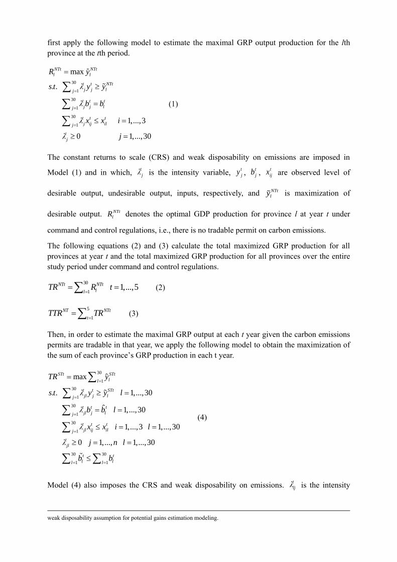
first apply the following model to estimate the maximal GRP output production for the lth

province at the tth period.

30

1

30

1

30

1

max

. .

1,...,3

0 1,...,30

NTt NTt

l l

t t NTt

j j lj

t t t

j j lj

t t t

j ij ilj

t

j

R y

s t λ y y

λ b b

λ x x i

λ j

=

=

=

=

=

=

=

(1)

The constant returns to scale (CRS) and weak disposability on emissions are imposed in

Model (1) and in which, t

jλ is the intensity variable, t

jy , t

jb , t

ijx are observed level of

desirable output, undesirable output, inputs, respectively, and NTt

ly is maximization of

desirable output. NTt

lR denotes the optimal GDP production for province l at year t under

command and control regulations, i.e., there is no tradable permit on carbon emissions.

The following equations (2) and (3) calculate the total maximized GRP production for all

provinces at year t and the total maximized GRP production for all provinces over the entire

study period under command and control regulations.

30

11,...,5NTt NTt

llTR R t

== = (2)

5

1

NT NTt

tTTR TR

== (3)

Then, in order to estimate the maximal GRP output at each t year given the carbon emissions

permits are tradable in that year, we apply the following model to obtain the maximization of

the sum of each province’s GRP production in each t year.

30

1

30

1

30

1

30

1

30 30

1 1

max

. . 1,...,30

1,...,30

1,...,3 1,...,30

0 1,..., 1,...,30

STt STt

ll

t t STt

jl j lj

t t t

jl j lj

t t t

jl ij ilj

t

jl

t t

l ll l

TR y

s t λ y y l

λ b b l

λ x x i l

λ j n l

b b

=

=

=

=

= =

=

=

= =

= =

= =

(4)

Model (4) also imposes the CRS and weak disposability on emissions. t

ljλ is the intensity

weak disposability assumption for potential gains estimation modeling.

variable, t

jy , t

jb , t

ijx are observed level of desirable output, undesirable output, inputs,

respectively. STt

ly is maximization of desirable output, t

lb is tradable undesirable output,

and both of them are variables. STtTR denotes the sum of the optimal GRP production for all

30 province at year t when spatial tradable permits are implemented. It should be noticed that

the last constraint in Model (4) indicates that the sum of the tradable undesirable output,

30

1

t

llb

= , should not exceed the aggregate allowed undesirable output emissions, 30

1

t

llb

= ,

which is the observed total amount of emissions subject to tradable permits in year t. This

observed total amount of carbon emissions also equals to the national total carbon emissions

under command and control scheme, since we take the command and control scheme as the

baseline for estimating the potential gains from trading.

The following Equations (5) and (6) calculate the maximized GRP production for each

province at year t and the total maximized GRP production for all provinces over the entire

study period with the spatial tradable permits in each year.

1,...,30 1,...,5STt STt

l lR y l t= = = (5)

5

1

ST STt

tTTR TR

== (6)

To estimate the maximal GRP output when the carbon emissions permit is tradable not just

among provinces but also over years during the entire period, the following model is applied.

5 30

1 1

30

1

30

1

30

1

5 30 30

1 1 1 1

max

. .

1,...,30 1,...,5

1,...,3 1,...,30 1,...,5

0 1,...,30 1,...,30 1,...,5

STT STTt

lt l

t t STTt

jl j lj

t t t

jl j lj

t t t

jl ij ilj

t

jl

t t

l lt l t l

TTR y

s t λ y y

λ b b l t

λ x x i l t

λ j l t

b b

= =

=

=

=

= = = =

=

= = =

= = =

= = =

5

(7)

The CRS and weak disposability on emissions settings, the variable of t

ljλ , and the parameters

of t

jy , t

jb , t

ijx in Model (7) are similar to those in the above two Models (1) and (4). In

addition, variables of STTt

ly and t

lb are maximization of desirable output and tradable

undesirable output, respectively. STTTTR denotes the sum of the optimal GRP production for

all 30 province over all year during the entire study period when spatial-temporal tradable

permits are implemented, i.e., to deposit and to borrow carbon emissions permits are allowed.

Similarly, the last constraint in Model (7) indicates that the sum of the tradable undesirable

output, 5 30

1 1

t

lt lb

= = , should less than or at least equal to the aggregate allowed undesirable

output emissions, 5 30

1 1

t

lt lb

= = , which is the observed total amount of emissions subject to

tradable permits during the entire study period that cover all 5 years. This observed total

amount carbon emissions also equals to the 5 years national total carbon emissions under

command and control scheme.

The last two Equations (8) and (9) calculate the maximized GRP production for each province

at year t and the total maximized GDP production for all provinces at year t with the

spatial-temporal tradable permits over the entire study period.

1,...,30 1,...,5STTt STTt

l lR y l t= = = (8)

30

11,...,5STTt STTt

llTR TR t

== = (9)

It should be noticed that, same as Färe et al. (2013, 2014), Models (1) and (4) are considered

contemporaneous approach in which each province is benchmarked against those provinces

that belong to the same year, and thus each year has its own production possibility set.

Moreover, Model (7) covers all provinces over the entire study period and thus it has a

combined production possibility set that each province in each year is benchmarked against a

unified efficiency frontier.

Models (1), (4) and (7) presented above are based on linear programming that the CRS

assumption is applied. In order to give greater flexibility to these models, the assumption of

variable returns to scale (VRS) is also applied and the corresponding models can be found in

the Appendix. We emphasis that since the VRS assumption is not directly linked with weak

disposability assumption (Färe and Grosskopf 2003; Kuosmanen, 2005; Zhou et al., 2008;

Murty et al., 2012) which is utilized for modeling CO2 emissions in this study, the DEA based

potential gains estimation models that satisfy these two assumptions need to be specifically

formulated by utilizing an addition abatement factor which keeps proportional reductions on

both desirable and undesirable outputs (Picazo-Tadeo and Prior, 2009). This specific

formulation leads a nonlinear programming (although could be linearized efficiently) and

complicates the estimation process. In addition, as pointed by several recent studies (e.g.

Aparicio et al., 2013; Hampf and Krüger, 2014), the utilization of weak disposability

assumption may lead to part of the frontier of the desirable and undesirable output set exhibits

a negative slope. This may lead to a situation that inefficient observations located on this part

are identified as efficient ones. To avoid this problem, we follow the concept of Aparicio et al.

(2013) in which a nested output set is utilized. However, the limitation of this approach is the

VRS model has not been derived. Therefore, in this study, the ex post estimation and analysis

is mainly based on CRS models. Note that, in recent study of carbon emissions abatement

allocation (Feng et al., 2015), the desirable GDP output is concave with respect to the

undesirable carbon emissions output, however, in the current study, this property is not in our

estimation of Model (1) since the nested output set is applied as mention above.

To summarize, NTtR (no tradable permit estimation or command and control estimation)

calculates the maximum GDP production when technical inefficiency is eliminated, and thus

we define NTtR y− as the Type I potential gains which identifies the potential desirable

output increase associated with eliminating inefficiency. STtR (spatial tradable permit

estimation) calculates the maximum GDP production when technical inefficiency is

eliminated, suboptimal spatial allocation of carbon emissions permit is eliminated, and gains

from spatial trading are allowed. Thus, STt NTtR R− can be defined as the Type II potential

gains which identifies the potential desirable output increase associated with eliminating

regulatory rigidity through allowing the trade of carbon emissions permits among different

regions within each single year. STTtR (spatial-temporal tradable permit estimation)

calculates the maximum GRP production when technical inefficiency is eliminated, both

suboptimal spatial and suboptimal temporal allocation of carbon emissions permits are

eliminated, and gains from spatial-temporal trading are allowed. Therefore, STTt STtR R− is

defined as the Type III potential gains identifying the potential desirable output increase

associated with eliminating regulatory rigidity through additionally allowing the trade of

carbon emissions permits over different period, i.e., the intertemporal depositing and

borrowing of carbon emissions permits are allowed. In this study, Type II and III potential

gains represent the estimated carbon abatement cost savings or carbon control leaded GRP

loss recoveries from implementing interprovincial and intertemporal carbon emissions trading

policy instruments instead of command and control policies on carbon emissions control.

4 Data

For calculating the potential gains from carbon emissions trading in China, we collect the

regional data from 2006-2010 which covers the 11th Five-Year-Plan (FYP) period. During this

period, the Chinese government proposed and implemented series of regulations and policies

for energy conservation and related carbon emissions control (Wang et al., 2012), and these

efforts have played a role in eliminating the inefficiency of energy utilization and carbon

emissions. In specific, during this period, a national energy intensity reduction target was

proposed and disaggregated, and each province of China has to reduce it energy intensity by

16%-22% within five years so as to realize the national target. These energy intensity

reduction targets are tightly interrelated with carbon emissions control regulations and thus

could also be seen as command and control regulations on carbon emissions. However, during

this period, market based regulatory strategy of tradable permits program for carbon

emissions was not implemented as a scheme for controlling carbon emissions in China.

Therefore, the calculation based on the data of this period will help to answer the question

that what are the potential gains or abatement cost savings from trade if the national carbon

emissions trading system is established in China during the 11th FYP period. In our estimation,

China’s 30 provinces over 5 years are the observations and, it should be noticed that, due to

interprovincial commuting and trade, not all of the provinces are absolute economically

independent, i.e., there may be neighborhood effects that the provinces are influenced with

each other. In order to reduce efficiency evaluation bias caused by neighborhood effects, DEA

based efficiency measure can at best be considered as short run evaluation instead of long run

evaluation from practical point of view, and thus we consider that 5 year length study period

in our estimation is appropriate.

As mentioned above, in this study, we use one desirable output y (GRP production), one

undesirable output b (carbon emissions), and three input x1 to x3 (energy consumption,

number of labor and capital stock) for calculation. The data on labor and the GRP are

obtained from China Statistical Yearbooks (2007-2011). The capital stock data are obtained

from Shan (2008) and our estimation (Wang et al., 2013b) through the perpetual inventory

method. The data on energy consumption3 are collected from China Energy Statistical

Yearbook. Since there are no official statistics on CO2 emissions at the regional level in China,

we estimate the CO2 emissions from fossil fuel consumptions. Firstly, the fossil fuel

consumptions4 (including the final consumptions and the consumptions in conversion) are

converted into calorific value according to the conversion factors (NBS, 2013). Then, they are

further translated into CO2 emissions according to the carbon emissions factors (IPCC, 2006)

and oxidation rate. The monetary GRP data and capital stock data have been converted into

2010 constant price and the energy consumption data has been converted into tonnes of coal

equivalent (tce), i.e., standard coal equivalent, according to the conversion factors provided in

China Energy Statistical Yearbook. The data set consists of 30 provinces over 5 years.

Summary statistics for each year during the study period are reported in Table 1.

[Insert Table 1 here]

5 Results and analysis

Model (1) and Equations (2) and (3) are first employed to estimate the maximal GRP output

for each province at each year under the command and control regulation that each province

seeks to maximize its GRP production with the observed levels of carbon emissions. If a

higher GRP output is identified than the observed GRP output, it means that there exists

technical inefficiency for the province under estimation. The difference between the maximal

GRP output and the observed GRP output ( NTtR y− ) represents the Type I potential gains

from eliminating technical inefficiency. Then, Model (4) and associated Equations (5) and (6)

are employed to estimate the Type II potential gains ( STt NTtR R− ) from eliminating spatial

regulatory rigidity, i.e., allowing carbon emissions permits to be traded spatially across

different province in a given year. The Type II potential gains represent the unrealized gains

from not allowing the reallocation of carbon emissions permits among provinces. Finally,

Model (7) and related Equations (8) and (9) are employed to calculate the Type III potential

gains ( STTt STtR R− ) from additionally eliminating temporal regulatory rigidity, that is, to allow

3 In this study, energy consumption indicates the total energy consumption but excludes the consumption in conversion of

the primary energy into the secondary energy and the loss in the process of conversion. 4 Including raw coal, cleaned coal, other washed coal, briquettes, coke, coke oven gas, other gas, crude oil, gasoline,

kerosene, diesel oil, fuel oil, liquefied petroleum gas, refinery gas, and natural gas.

carbon emissions permits to be traded not only across regions but also across period. In other

words, the permits for carbon emissions are both tradable and allowed to be deposited and

borrowed. The summation of Type II and III potentials gains from the trade of carbon

emissions constitute the upper limit on the potential cost of transaction of the permits.

Furthermore, the carbon emissions reduction potentials (t t

l lb b− , 30 30

1 1

t t

l ll lb b

= =− and

5 30 5 30

1 1 1 1

t t

l lt l t lb b

= = = =− ) from spatial and temporal trading also can be calculated based on

the optimal solutions of Models (1), (4) and (7), respectively, and the total amount of carbon

emissions reduction potential also represents the effectiveness of carbon emissions control

caused by introducing carbon emissions trading scheme in China.

Table 2 first reports the percentage of annual potential gains from trade of carbon emissions in

China. The second column is the percentage of Type I potential gains over the observed GRP

production, the third column shows the percentage of Type II potential gains over the

maximized GRP with command and control estimations, and the fourth columns shows the

percentage of Type III potential gains over the maximized GRP with spatial tradable permits.

In addition, Table 2 also reports the percentage of annual carbon emissions reduction

potentials from trade of carbon emissions in China. The fifth and sixth column respectively

represents the percentage of carbon emissions reduction associated with the realization of

Type II and III potential gains when spatial trading and spatial-temporal trading scheme is

implemented.


The percentage of annual Type I potential gains ranges from 4.37% to 7.60% during

2006-2010 which indicates a considerable amount of theoretical GDP loss associated with

technical inefficiency of China, i.e., the theoretical GDP loss due to the fact that not all the

provinces were operating on the efficiency frontier. During the same period, the annual Type

II and III potential gains represent the differences in maximal GDP production between the no

tradable permit or command and control GDP estimations and the tradable permit GDP

estimations in China. The percentage of annual Type II potential gains ranges from 8.32% to

13.50% and the percentage of annual Type III potential gains ranges from 2.74% to 8.33%,

which respectively represent the theoretical magnitude of GDP loss associated with the spatial

regulatory rigidity and the temporal regulatory rigidity of China, i.e., the theoretical GDP

losses due to the suboptimal allocation of carbon emissions permits among provinces and

over years.

For the observed inputs of energy, labor and capital unchanged, and the technology fixed

during the study period, the positive Type II to Type III potential gains support our

expectation that less flexibility on regulations (or high rigidity on regulations) would lead to

reduction on GDP production, and thus the introduction of carbon emissions trading system

would help to realize the potential GDP production in China, or in other words, to implement

carbon emissions trading scheme would help to reduce the GDP loss due to the command and

control policies on carbon emissions in which the carbon emissions permits are not able to be

optimally reallocated among provinces in China.

The results reported in Table 2 also respectively reveal an average increase potential on GDP

of 5.87%, 10.78% and 5.96% for China over the period of 2006-2010 if the technical

inefficiency, the intra-period carbon emissions allocation inefficiency, and the inter-period

carbon emissions allocation inefficiency could be eliminated. This result indicates that the

GDP loss caused by carbon emissions control in China during 2006-2010 can be recovered by

approximate 17% (summation of Type II and III potential gains) through implementing

interprovincial and additionally intertemporal carbon emissions trading schemes.

Fig. 1 illustrates three types of annual potential gains from carbon emissions permits trade of

China during 2006-2010. It can be found that, on average, the Type II and III potential gains

together account for approximate 75% of total GDP increase potentials or GDP loss

recoveries in China, in which, 46% of the potential gains (Type II) could be realized through

eliminating the rigidity of spatial trading, and 29% of the potential gains (Type III) could be

achieved by eliminating the temporal trading rigidity. The remaining 25% of total GDP

increase potential comes from reducing technical inefficiency.

[Insert Figure 1 here]

Table 2 also reports the potentials on carbon emissions reduction in China from the trade of

carbon emissions permits over 2006-2010. When the spatial tradable emissions permits are

implemented, an average carbon emissions reduction percentage of 10.97% compared with

the observed or command and control carbon emissions can be identified. And if the

additional spatial-temporal tradable emissions permits are implemented, an average carbon

emissions reduction percentage of 2.36% compared with the spatial tradable carbon emissions

can be additionally realized. Note that, for each single year under estimation, China’s carbon

emissions could be reduced from spatial and spatial-temporal permits trading. There is only

one exception that, in 2006, carbon emissions increased 1%. This indicates that if

spatial-temporal permits trading are allowed, some provinces may borrow additional permits

from themselves or other provinces in the remaining years and emit more CO2 than observed

values in 2006 so as to achieve more GRP outputs.

Fig. 2 further illustrates the difference between the observed carbon emissions and the carbon

emissions with spatial and temporal tradable permits of China from 2006 to 2010. It is notable

that, the introduction of carbon emissions permits trading scheme will not only lead to

potential GDP increase or reduce GDP loss caused by command and control policies, but also

help to reduce total carbon emissions in China, and on average, most of the reduction

potentials come from spatial trading (84%) with a small amount of potentials come from

additional spatial-temporal trading (16%).


The realization of Type II and III potential gains or GDP loss recoveries from carbon

emissions trading, and the realization of associated carbon emissions reduction potentials in

China during 2006-2010 should be explained by the reallocation of carbon emissions

reduction burdens from the provinces with high carbon emissions inefficiencies and high

abatement costs to those provinces with low inefficiencies and low costs. In this study, we

have 150 observations, i.e., 30 provinces with 5 years, under estimation, and the five years

average of potential gains and carbon emissions reduction potentials of these 30 provinces are

reported (both in percentages) in Table 3. It can be seen that Qinghai, Jilin and Ningxia

respectively present the highest percentages on Type I, II and III potential gains.


According to the percentages of Type I potential gains, which account the GRP increase

percentages from eliminating technical inefficiencies of specific provinces in China, we could

find that the efficiency difference in the production process of desirable and undesirable

outputs in China among different regions is substantial, since the economic well-developed

regions, such as Beijing, Shanghai, and Guangdong etc., always produced on the efficiency

frontier and show no Type I potential gains, but the underdeveloped regions like Qinghai,

Gansu and Yunnan etc. kept suffering from high technical inefficiencies in their production

processes and show high percentages on Type I potential gains (24-36%).

According to the combined percentages of Type II and III potential gains, which account the

GRP increase percentages from spatial and temporal trading of carbon emissions permits, Jilin

shows the highest gains (51%) followed by Ningxia (42%) and Hebei (36%). Guangdong

presents the lowest gains (0.04%) followed by Inner Mongolia (0.6%) and Shanghai (1.9%).

Although the deviation on the percentage of potential gains is relatively large, all provinces

shows positive potential gains from carbon emissions trading. Furthermore, among all 30

provinces, 26 provinces present carbon emissions reduction potentials, in which Hainan has

the highest average reduction percentage (32%), followed by Jilin (31%) and Hebei (31%),

and Inner Mongolia has the lowest average reduction percentage (0.8%). The remaining four

provinces (Guangdong, Chongqing, Shanghai and Xinjiang) which have negative reduction

percentage values may increase their carbon emissions after trading. This indicates that if the

spatial and temporal permit trading is allowed, in aggregate, Guangdong, Chongqing,

Shanghai and Xinjiang will be the buyers of carbon emissions permits over the entire study

period of 2006-2010. Although, these four provinces may increase their emissions, the total

amount is just 23.39 million tonnes which is quite lower than the total amount of carbon

emissions reduction potentials of the other 26 provinces (981.1 million tonnes). Fig. 3 further

illustrates the cluster map of China’s provinces with different percentages of combined Type

II and III potential gains from carbon emissions trading.


We further compare the observed carbon emissions intensity reduction during 2006-2010 (11th

FYP period) with the estimated carbon emissions intensity if the technical inefficiency and the

inefficiency of suboptimal allocation of emissions permits are eliminated, i.e., three types of

potential gains from trade are realized, so as to highlight the effectiveness of introducing

carbon emissions trading programs from the perspective of reducing China’s carbon

emissions intensity.


The results in column 2 of Table 4 report the observed carbon intensity reduction percentage

of China and its 30 province of 2010 compared with 2006, which revels a 19.7 percent

decrease at the national level. This reduction is due to Chinese government’s effort on

implementing energy conservation and emissions reduction policies and regulations during

the 11th FYP period (Wang et al., 2013a). If the technical inefficiency of the province, which

is not located on the production frontier, is eliminated, the estimation results in column 3 revel

that there will be another 5% carbon intensity reduction potential would be realized at the

national level, and the reduction percentages for those inefficient provinces range from 1%

(Zhejiang) to 27% (Qinghai). The last two columns of Table 4 report the estimated carbon

intensity reduction percentages from spatial trading and spatial-temporal trading, respectively.

It is obvious that, at the national level, approximate 20% of the potential reduction could be

realized through eliminating spatial rigidity and another 7% reduction potential could be

realized through eliminating temporal rigidity. Both of the carbon intensity reduction

potentials caused by emissions trading are higher than that due to improving technical

inefficiency. Among all China’s 30 provinces, there are respectively 21 provinces and 27

provinces show carbon intensity reduction potentials from spatial trading and spatial-temporal

trading, and their reduction percentages range from 1%-53% and 1%-30%, respectively.

These results imply that, the elimination of trading rigidity of carbon emissions permits will

help to release more carbon intensity reduction potentials than command and control or no

tradable permit policies on carbon emissions for all provinces in China that participated in the

trading system. These estimation results are further illustrated in Fig. 4.


As discussed above, the major attraction of provincial carbon emissions permits trading in

China is its potential to achieve stated emissions control target (e.g. 17% decrease in carbon

emissions intensity during 2010-2015), and to achieve this target at lower cost than that if

each province faces individual carbon emission reduction burden. This study indicates that, in

a spatial and temporal permits trading system, provinces that face relatively high emissions

reduction costs (e.g. Shanghai and Guangdong) could purchase additional emissions permits

from other provinces rather than incur the high costs, and correspondingly, provinces that are

capable to reduce carbon emissions at relatively low costs (e.g. Hebei and Shandong) could

have choices to purchase fewer permits or sell excess permits. Although these choices oblige

these provinces to reduce carbon emissions further, their avoided abatement costs or permits

sale revenues will compensate the costs associated with extra emissions reductions. This will

provide a constant incentive of each province to identify cost minimizing abatement

opportunities.

Moreover, the carbon emissions permits trading system provide Chinese government, the

environmental regulation authority, considerable flexibility to distribute net carbon abatement

compliance costs across covered regions (30 provinces in mainland China except for Tibet

which was not assigned energy and carbon intensity reduction targets during 11th and 12th

FYP periods). Since the emissions permits become valuable assets, the government will have

the ability to reduce or even offset the cost of emissions permits trading program through

using the value of permits to benefit those provinces that have purchased them, and the

government also can use this value to achieve development goals such as protect the jobs of

coal miners and coal-fired power industry workers in provinces with rich coal endowments

(e.g. Shanxi and Shaanxi), to provide additional protections for China’s western low-income

provinces (e.g. Yunnan and Guizhou), and to incentive high-income provinces (e.g. Jiangsu

and Zhejiang) to investment more in abatement technology and procedure. Furthermore, the

cost saving effect of carbon emissions permits trading identified in this study could

additionally strengthen the case for marketable permits trading for controlling other pollutants

(through pollutant trading) and energy consumptions (through energy saving quantity trading)

in China.

6 Conclusions

Carbon emissions permit trading is known as a market based regulatory scheme for reducing

greenhouse gas emissions cost-effectively. China has just recently launched its carbon trading

markers in seven pilot regions. In this study, we try to answer the question that what will be

the abatement cost savings or GDP loss recoveries from carbon emissions trading in China

from the perspective of estimating the potential gains from carbon emissions trading. Through

an ex post analysis based on China’s provincial data over 2006-2010 and by applying a DEA

based optimization model with several trading schemes, this study estimates three types (Type

I, II and III) of potential gains from (i) eliminating technical inefficiency under the no tradable

permit scheme or command and control regulation, (ii) implementing spatial tradable permit

scheme on carbon emissions, and (iii) implementing spatial-temporal tradable permit scheme

on carbon emissions in China. The Type I potential gains calculate the potential GDP increase

associated with eliminating technical inefficiency on GDP production and carbon emissions

under the carbon emissions command and control or no tradable permit scheme. If a spatial

tradable carbon emissions permit system exists in China, the Type II potential gains identifies

the potential GDP increase or GDP loss recovery associated with reducing spatial regulatory

rigidity by eliminating intra-period carbon emissions allocation inefficiency. In addition, the

Type III potential gains identifies, if a spatial-temporal tradable carbon emissions permits

system exists in China, the additional potential GDP increase or GDP loss recovery associated

with reducing temporal regulatory rigidity by eliminating inter-period carbon emissions

allocation inefficiency. Type II and III potential gains together identify the potential increase

in GDP production, or in other words, the recovery in GDP loss, if an efficient spatial and

temporal tradable carbon emissions permits scheme is implemented instead of the carbon

emissions command and control policies in China. Our estimation results can be concluded as

follows.

i) China’s 30 provinces have various economic growth modes, natural resource endowments,

energy consumption patterns, industrial structures, and technological levels, and this

heterogeneity gives rise to diversified carbon emissions abatement costs in different provinces.

The difference in carbon abatement cost determines the efficiency advantage of market based

instruments as carbon emissions trading over command and control policies and this

advantage is realized in the form of potential gains or potential cost savings from emissions

permits trading. This study indicates substantial potential cost savings from carbon emissions

permits trading in China.

ii) The average percentage on potential gains of Type I, II and III is 5.87%, 10.78% and

5.96%, respectively, in China over the period of 2006-2010. The considerable large magnitude

of potential gains identified in this study supports the expectation that less flexibility on

emission trading regulations leads to reduction on GDP output. Therefore, the implementation

of carbon emissions permit trading program in China will contribute to realize the potential

gains, or in other words, the carbon emissions control leaded GDP loss in China can be

recovered through implementing interprovincial and intertemporal carbon emissions trading

schemes.

iii) About 75% of the theoretical GDP loss in China during 2006-2010 is due to the regulation

rigidity of not allowing spatial and temporal trading of carbon emissions permits, and in

which, 46% and 26% of the potential gains could be realized through eliminating the spatial

trading rigidity and temporal trading rigidity, respectively. The remaining 25% GDP loss is

due to technical inefficiency of GDP production and carbon emissions of specific provinces in

China.

iv) The implementation of carbon emissions permit trading program will also help to reduce

total carbon emissions in China. The average carbon emissions reduction percentages are

10.97% and 2.36% if the interprovincial trading scheme and the additional intertemporal

trading scheme are implemented, respectively.

iv) All China’s 30 provinces under estimation could have potential gains or benefit from

reducing GDP loss through carbon emissions trading, and according to the combination of

Type II and III potential gains, Jilin shows the highest percentage on GDP loss recovery

(50%). In addition, 26 out of 30 provinces present carbon emissions reduction potentials from

trading, and in which, Hainan has the highest percentage on carbon emissions reduction

potential (34%).

v) The elimination of rigidity on carbon emissions permit trading will also release additional

carbon emissions intensity reduction potentials in China, and all China’s provinces that

participate in the trading scheme will benefit from additionally reducing their carbon

emissions intensities by 8%-56%.

vi) A marketable carbon permits trading would provide the entities covered a constant

incentive to identify cost minimizing abatement opportunities, and provide Chinese

government the flexibility in determining the distribution of abatement cost savings for

achieving further economic and social development goals.

Acknowledgement

The authors gratefully acknowledge the financial support from the National Natural Science

Foundation of China (grant nos. 71471018 and 71101011) and the Outstanding Young

Teachers Foundation of Beijing Institute of Technology (grant no. 2013YR2119).

Appendix

The variable returns to scale DEA models for identifying potential gains from trade are

presented as follows in Models (A1) to (A4), in which the abatement factor θj and θjl are

applied to keep the reductions of desirable and undesirable outputs proportionally. The

explanations of other parameters and variables in Models (A1) to (A4) are same with Models

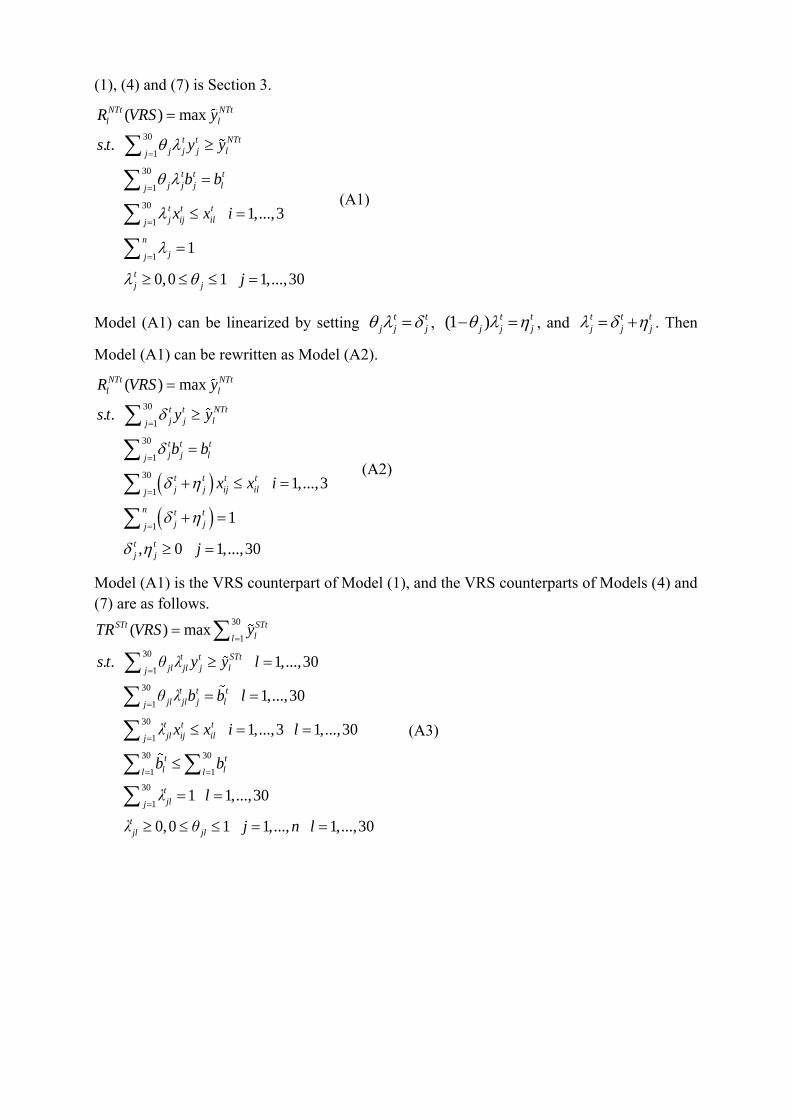
(1), (4) and (7) is Section 3.

30

1

30

1

30

1

1

( ) max

. .

1,...,3

1

0,0 1 1,...,30

NTt NTt

l l

t t NTt

j j j lj

t t t

j j j lj

t t t

j ij ilj

n

jj

t

j j

R VRS y

s t y y

b b

x x i

j

=

=

=

=

=

=

=

=

=

(A1)

Model (A1) can be linearized by setting t t

j j j= , (1 ) t t

j j j− = , and t t t

j j j= + . Then

Model (A1) can be rewritten as Model (A2).

( )

( )

30

1

30

1

30

1

1

( ) max

. .

1,...,3

1

, 0 1,...,30

NTt NTt

l l

t t NTt

j j lj

t t t

j j lj

t t t t

j j ij ilj

n t t

j jj

t t

j j

R VRS y

s t y y

b b

x x i

j

=

=

=

=

=

=

+ =

+ =

=

(A2)

Model (A1) is the VRS counterpart of Model (1), and the VRS counterparts of Models (4) and

(7) are as follows. 30

1

30

1

30

1

30

1

30 30

1 1

30

1

( ) max

. . 1,...,30

1,...,30

1,...,3 1,...,30

1 1,...,30

0,0 1 1,..., 1

STt STt

ll

t t STt

jl jl j lj

t t t

jl jl j lj

t t t

jl ij ilj

t t

l ll l

t

jlj

t

jl jl

TR VRS y

s t θ λ y y l

θ λ b b l

λ x x i l

b b

λ l

λ θ j n l

=

=

=

=

= =

=

=

=

= =

= =

= =

= =

,...,30

(A3)

5 30

1 1

30

1

30

1

30

1

5 30 5 30

1 1 1 1

30

1

( ) max

. .

1,...,30 1,...,5

1,...,3 1,...,30 1,...,5

1 1,...,30

STT STTt

lt l

t t STTt

jl jl j lj

t t t

jl jl j lj

t t t

jl ij ilj

t t

l lt l t l

t

jlj

TTR VRS y

s t θ λ y y

θ λ b b l t

λ x x i l t

b b

λ l

= =

=

=

=

= = = =

=

=

= = =

= = =

= =

0,0 1 1,...,30 1,...,30 1,...,5t

jl jlλ θ j l t = = =

(A4)

The linearization of Models (A3) and (A4) are similar with Model (A2) and are omitted here.

Reference

Aparicio, J., Pastor, J. T., Zofio, J. L. (2013). On the inconsistency of the Malmquist–

Luenberger index. European Journal of Operational Research, 229(3), 738-742.

Carlson, C., Burtraw, D., Cropper, M., & Palmer, K. L. (2000). Sulfur dioxide control by

electric utilities: What are the gains from trade? Journal of Political Economy, 108(6),

1292-1317.

Chan, G, Stavins, R. N., Stowe, R., & Sweeney, R. (2012). The SO2 allowance trading system

and the clean air act amendments of 1990: Reflections on twenty years of policy innovation.

Faculty ResearchWorking Paper Series, John F. Kennedy School of Government, Harvard

University.

Chen, L., Zhang, B., Hou, H., & Taudes, A. (2013). Impact Study of Carbon Trading Market

to Highway Freight Company in China. In LTLGB 2012 (pp. 347-353). Springer Berlin

Heidelberg.

Cong, R. G., & Wei, Y. M. (2010). Potential impact of (CET) carbon emissions trading on

China’s power sector: A perspective from different allowance allocation options. Energy,

35(9), 3921-3931.

Cook, W. D., & Zhu, J. (2014). Data Envelopment Analysis: A Handbook on the Modeling of

Internal Structures and Networks. Springer US.

Cook, W. D., Tone, K., & Zhu, J. (2014). Data envelopment analysis: prior to choosing a

model. Omega, 44, 1-4.

Cooper, W. W., Seiford, L. M., & Zhu, J. (2011). Handbook on data envelopment analysis

(Vol. 164). Springer Science & Business Media.

Cui, L. B., Fan, Y., Zhu, L., & Bi, Q. H. (2014). How will the emissions trading scheme save

cost for achieving China’s 2020 carbon intensity reduction target? Applied Energy, 136,

1043-1052.

Färe, R., & Grosskopf, S. (2003). Nonparametric productivity analysis with undesirable

outputs: comment. American Journal of Agricultural Economics, 85(4), 1070-1074.

Färe, R., Grosskopf, S., Lovell, C. K., & Pasurka, C. (1989). Multilateral productivity

comparisons when some outputs are undesirable: a nonparametric approach. The review of

economics and statistics, 90-98.

Färe, R., Grosskopf, S., & Pasurka Jr, C. A. (2013). Tradable permits and unrealized gains

from trade. Energy Economics, 40, 416-424.

Färe, R., Grosskopf, S., & Pasurka Jr, C. A. (2014). Potential gains from trading bad outputs:

The case of US electric power plants. Resource and Energy Economics, 36(1), 99-112.

Feng, C., Chu, F., Ding, J., Bi, G., & Liang, L. (2015). Carbon Emissions Abatement (CEA)

allocation and compensation schemes based on DEA. Omega, 53, 78-89.

Goulder, L. H., & Schein, A. R. (2013). Carbon tax versus cap and trade: A Critical review.

Climate Change Economics, 4(3), 1-28.

Hailu, A., & Veeman, T. S. (2001). Non-parametric productivity analysis with undesirable

outputs: an application to the Canadian pulp and paper industry. American Journal of

Agricultural Economics, 83(3), 605-616.

Hampf, B., & Krüger, J. J. (2015). Optimal Directions for Directional Distance Functions: An

Exploration of Potential Reductions of Greenhouse Gases. American Journal of Agricultural

Economics, 97(3), 920-938.

Huang, Y., Liu, L., Ma, X., & Pan, X. (2015). Abatement technology investment and

emissions trading system: a case of coal-fired power industry of Shenzhen, China. Clean

Technologies and Environmental Policy, 17(3), 811-817.

Hübler, M., Voigt, S., & Löschel, A. (2014). Designing an emissions trading scheme for

China - An up-to-date climate policy assessment. Energy Policy,75, 57-72.

IPCC. (2006). IPCC Guidelines for National Greenhouse Gas Inventories: Volume II Energy.

Institute for Global Environmental Strategies, Japan.

Jiang, J. J., Ye, B., & Ma, X. M. (2014). The construction of Shenzhen׳ s carbon emission

trading scheme. Energy Policy, 75, 17-21.

Jotzo, F., & Löschel, A. (2014). Emissions trading in China: Emerging experiences and

international lessons. Energy Policy, 75, 3-8.

Kuosmanen, T. (2005). Weak disposability in nonparametric production analysis with

undesirable outputs. American Journal of Agricultural Economics, 87(4), 1077-1082.

Li, J. F., Wang, X., Zhang, Y. X., & Kou, Q. (2014). The economic impact of carbon pricing

with regulated electricity prices in China - An application of a computable general

equilibrium approach. Energy Policy, 75, 46-56.

Liu, Y., Feng, S., Cai, S., Zhang, Y., Zhou, X., Chen, Y., & Chen, Z. (2013). Carbon emission

trading system of China: a linked market vs. separated markets. Frontiers of Earth Science,

7(4), 465-479.

Liu, Y., & Wei, T. (2014). Linking the emissions trading schemes of Europe and

China-Combining climate and energy policy instruments. Mitigation and Adaptation

Strategies for Global Change, 10.1007/s11027-014-9580-5.

Lovell, C. A. K., Pastor, J. T., & Turner, J. A. (1995). Measuring macroeconomic

performance in the OECD: a comparison of European and non-European countries. European

Journal of Operational Research, 87(3), 507-518.

Lozano, S., Villa, G., & Brännlund, R. (2009). Centralised reallocation of emission permits

using DEA. European Journal of Operational Research, 193(3), 752-760.

Murty, S., Russell, R.R., & Levkoff, S.B. (2012). On Modeling Pollution-Generating

Technologies. Journal of Environmental Economics and Management, 64(1), 117-135.

NBS. (2013). China energy statistical yearbook. National Bureau of Statistics of People's

Republic of China (NBS), Beijing.

NDRC. (2014). Provisional regulation on carbon emissions trading management. National

Development and Reform Commission (NDRC), People’s Republic of China.

http://qhs.ndrc.gov.cn/zcfg/201412/t20141212_652007.html.

Ni, F. D., & Chan, E. H. (2014). Carbon Emission Trading Scheme to Reduce Emission in the

Built Environment of China. In Proceedings of the 17th International Symposium on

Advancement of Construction Management and Real Estate (pp. 317-325). Springer Berlin

Heidelberg.

Picazo-Tadeo, A.J., Prior, D. (2009). Environmental externalities and efficiency measurement.

Journal of Environmental Management, 90(11), 3332-3339.

Shan, H. J. (2008). Re-estimating the capital stock of China: 1952-2006, The Journal of

Quantitative & Technical Economics, 10, 17-31[in Chinese].

Seiford, L. M., & Zhu, J. (2002). Modeling undesirable factors in efficiency evaluation.

European Journal of Operational Research, 142(1), 16-20.

Seiford, L. M., & Zhu, J. (2005). A response to comments on modeling undesirable factors in

efficiency evaluation. European Journal of Operational Research, 161(2), 579-581.

Sueyoshi, T., & Goto, M. (2013). Returns to scale vs. damages to scale in data envelopment

analysis: An impact of US clean air act on coal-fired power plants. Omega, 41(2), 164-175.

Sun, J., Wu, J., Liang, L., Zhong, R.Y., & Huang, G.Q. (2014). Allocation of emission

permits using DEA: Centralised and individual points of view. International Journal of

Production Research, 52(2), 419-435.

Teng, F., Wang, X., & Zhiqiang, L. V. (2014). Introducing the emissions trading system to

China’s electricity sector: Challenges and opportunities. Energy Policy, 75, 39-45.

Wang, K., & Wei, Y. M. (2014) China’s regional industrial energy efficiency and carbon

emissions abatement costs. Applied Energy, 130, 617-631.

Wang, K., Wei, Y. M., & Zhang, X. (2012). A comparative analysis of China’s regional

energy and emission performance: Which is the better way to deal with undesirable outputs?

Energy Policy, 46, 574-584.

Wang, K., Wei, Y. M., & Zhang, X. (2013a). Energy and emissions efficiency patterns of

Chinese regions: a multi-directional efficiency analysis. Applied Energy, 104, 105-116.

Wang, K., Yu, S., & Zhang, W. (2013b). China’s regional energy and environmental

efficiency: a DEA window analysis based dynamic evaluation. Mathematical and Computer

Modelling, 58(5), 1117-1127.

Wang, K., Zhang, X., Wei, Y. M., & Yu, S. (2013c). Regional allocation of CO2 emissions

allowance over provinces in China by 2020. Energy Policy, 54, 214-229.

Wang, P., Dai, H. C., Ren, S. Y., Zhao, D. Q., & Masui, T. (2015). Achieving Copenhagen

target through carbon emission trading: Economic impacts assessment in Guangdong

Province of China. Energy 79, 212-227.

Wei, C., Ni, J., & Du, L. (2012). Document Regional allocation of carbon dioxide abatement

in China. China Economic Review, 23(3), 552-565.

Wei, Y. M., Mi, Z. F., & Huang, Z. (2014). Climate policy modeling: An online SCI-E and

SSCI based literature review. Omega, doi:10.1016/j.omega.2014.10.011.

Wu, H., Du, S., Liang, L., & Zhou, Y. (2013). A DEA-based approach for fair reduction and

reallocation of emission permits. Mathematical and Computer Modelling, 58(5-6),

1095-1101.

Wu, L., Qian, H., & Li, J. (2014). Advancing the experiment to reality: Perspectives on

Shanghai pilot carbon emissions trading scheme. Energy Policy, 75, 22-30.

Zhang, D., Karplus, V. J., Cassisa, C., & Zhang, X. (2014). Emissions trading in China:

Progress and prospects. Energy Policy, 75, 9-16.

Zhou, P., & Ang, B. W. (2008). Linear programming models for measuring economy-wide

energy efficiency performance. Energy Policy, 36(8), 2911-2916.

Zhou, P., Sun, Z. R., & Zhou, D. Q. (2014). Optimal path for controlling CO2 emissions in

China: A perspective of efficiency analysis. Energy Economics, 45, 99-110.

Zhou, P., Zhang, L., Zhou, D. Q., & Xia, W. J. (2013). Modeling economic performance of

interprovincial CO2 emission reduction quota trading in China. Applied Energy, 112,

1518-1528.

Zhu, B., & Wei, Y. (2013). Carbon price forecasting with a novel hybrid ARIMA and least

squares support vector machines methodology. Omega, 41(3), 517-524.

Zhu, J. (2014). Quantitative models for performance evaluation and benchmarking: data

envelopment analysis with spreadsheets (Vol. 213). Springer.

Zhu, Y., Li, Y. P., & Huang, G. H. (2013). Planning carbon emission trading for Beijing's

electric power systems under dual uncertainties. Renewable and Sustainable Energy Reviews,

23, 113-128.

Figures and Tables

Fig. 1 Potential gains from trade of China

Fig. 2 Carbon emissions reduction potentials from trade of China

0

2000

4000

6000

8000

10000

12000

14000

2006 2007 2008 2009 2010

Bil

lio

n Y

uan

Type III potential gains

Type II potential gains

Type I potential gains

0

2000

4000

6000

8000

10000

2006 2007 2008 2009 2010

Mil

lio

n t

on

ne

Observed carbon emissionsCarbon emissions with spatial-tradable permitsCarbon emissions with spatial-temporal-tradable permits

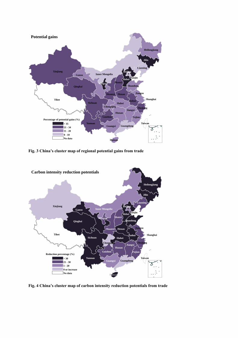
Fig. 3 China’s cluster map of regional potential gains from trade

Fig. 4 China’s cluster map of carbon intensity reduction potentials from trade

> 35

21 - 34

11 - 20

0 - 10

No data

Gansu

Qinghai

XinjiangInner Mongolia

Sichuan

Yunnan

Guizhou

Guangxi

Chongqing

Hunan

Guangdong

Jiangxi

Fujian

AnhuiHubei

HenanShaanxi

Shanxi

Shandong

Hebei

Beijing

Tianjin

Heilongjiang

Jilin

Liaoning

Tibet

Taiwan

Zhejiang

Jiangsu

Shanghai

Hainan

Ningxia

Potential gains

Percentage of potential gains (%)

Reduction percentage (%)

> 30

21 - 30

1 - 20

0 or increase

No data

Gansu

Qinghai

XinjiangInner Mongolia

Sichuan

Yunnan

Guizhou

Guangxi

Chongqing

Hunan

Guangdong

Jiangxi

Fujian

AnhuiHubei

HenanShaanxi

Shanxi

Shandong

Hebei

Beijing

Tianjin

Heilongjiang

Jilin

Liaoning

Tibet

Taiwan

Zhejiang

Jiangsu

Shanghai

Ningxia

Hainan

Carbon intensity reduction potentials

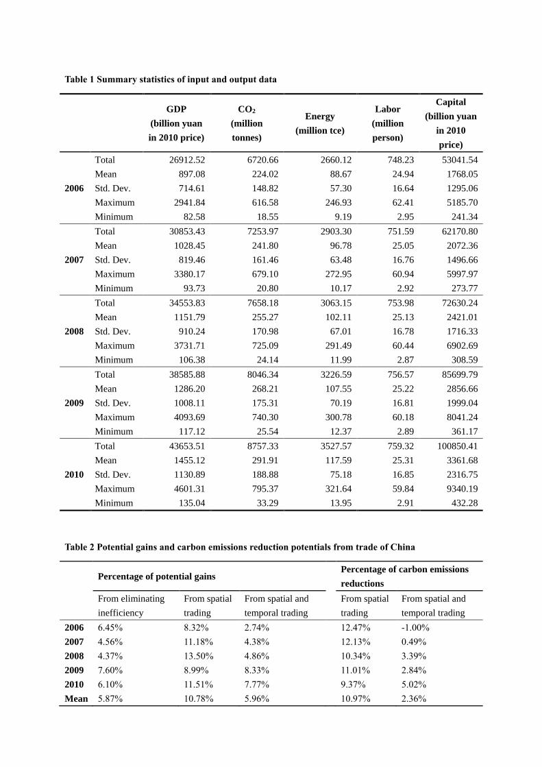
Table 1 Summary statistics of input and output data

GDP

(billion yuan

in 2010 price)

CO2

(million

tonnes)

Energy

(million tce)

Labor

(million

person)

Capital

(billion yuan

in 2010

price)

2006

Total 26912.52 6720.66 2660.12 748.23 53041.54

Mean 897.08 224.02 88.67 24.94 1768.05

Std. Dev. 714.61 148.82 57.30 16.64 1295.06

Maximum 2941.84 616.58 246.93 62.41 5185.70

Minimum 82.58 18.55 9.19 2.95 241.34

2007

Total 30853.43 7253.97 2903.30 751.59 62170.80

Mean 1028.45 241.80 96.78 25.05 2072.36

Std. Dev. 819.46 161.46 63.48 16.76 1496.66

Maximum 3380.17 679.10 272.95 60.94 5997.97

Minimum 93.73 20.80 10.17 2.92 273.77

2008

Total 34553.83 7658.18 3063.15 753.98 72630.24

Mean 1151.79 255.27 102.11 25.13 2421.01

Std. Dev. 910.24 170.98 67.01 16.78 1716.33

Maximum 3731.71 725.09 291.49 60.44 6902.69

Minimum 106.38 24.14 11.99 2.87 308.59

2009

Total 38585.88 8046.34 3226.59 756.57 85699.79

Mean 1286.20 268.21 107.55 25.22 2856.66

Std. Dev. 1008.11 175.31 70.19 16.81 1999.04

Maximum 4093.69 740.30 300.78 60.18 8041.24

Minimum 117.12 25.54 12.37 2.89 361.17

2010

Total 43653.51 8757.33 3527.57 759.32 100850.41

Mean 1455.12 291.91 117.59 25.31 3361.68

Std. Dev. 1130.89 188.88 75.18 16.85 2316.75

Maximum 4601.31 795.37 321.64 59.84 9340.19

Minimum 135.04 33.29 13.95 2.91 432.28

Table 2 Potential gains and carbon emissions reduction potentials from trade of China

Percentage of potential gains Percentage of carbon emissions

reductions

From eliminating

inefficiency

From spatial

trading

From spatial and

temporal trading

From spatial

trading

From spatial and

temporal trading

2006 6.45% 8.32% 2.74% 12.47% -1.00%

2007 4.56% 11.18% 4.38% 12.13% 0.49%

2008 4.37% 13.50% 4.86% 10.34% 3.39%

2009 7.60% 8.99% 8.33% 11.01% 2.84%

2010 6.10% 11.51% 7.77% 9.37% 5.02%

Mean 5.87% 10.78% 5.96% 10.97% 2.36%

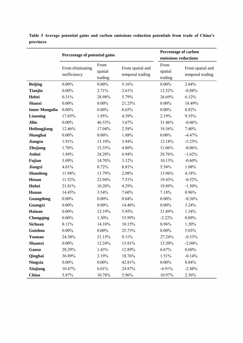
Table 3 Average potential gains and carbon emissions reduction potentials from trade of China’s

provinces

Percentage of potential gains Percentage of carbon

emissions reductions

From eliminating

inefficiency

From

spatial

trading

From spatial and

temporal trading

From

spatial

trading

From spatial and

temporal trading

Beijing 0.00% 0.00% 5.16% 0.00% 2.64%

Tianjin 0.00% 2.71% 2.61% 12.52% -0.88%

Hebei 0.31% 28.98% 5.79% 26.69% 6.12%

Shanxi 0.00% 0.00% 21.25% 0.00% 18.49%

Inner Mongolia 0.00% 0.00% 0.65% 0.00% 0.82%

Liaoning 17.65% 1.95% 4.39% 2.19% 9.35%

Jilin 0.00% 46.53% 3.67% 31.46% -0.06%

Heilongjiang 12.46% 17.04% 2.58% 19.36% 7.40%

Shanghai 0.00% 0.00% 1.88% 0.00% -4.47%

Jiangsu 1.91% 13.10% 3.94% 12.18% -5.25%

Zhejiang 1.70% 15.35% 4.80% 11.06% -0.06%

Anhui 1.84% 24.28% 6.94% 28.76% -1.62%

Fujian 5.09% 14.70% 3.12% 10.13% -0.60%

Jiangxi 4.01% 8.72% 8.81% 5.54% 1.08%

Shandong 11.94% 13.79% 2.08% 13.96% 4.18%

Henan 11.52% 22.94% 7.51% 19.43% -0.52%

Hubei 21.81% 10.20% 4.29% 19.89% -1.50%

Hunan 14.45% 3.54% 7.60% 7.18% 0.96%

Guangdong 0.00% 0.00% 0.04% 0.00% -0.36%

Guangxi 0.00% 0.00% 14.46% 0.00% 3.24%

Hainan 0.00% 12.19% 5.95% 31.89% 1.34%

Chongqing 0.00% 1.30% 15.99% -2.22% 0.09%

Sichuan 8.11% 14.10% 10.15% 8.96% 1.20%

Guizhou 0.00% 0.00% 25.73% 0.00% 5.03%

Yunnan 24.30% 21.15% 9.11% 27.24% -0.53%

Shaanxi 0.00% 12.24% 13.81% 13.20% -2.04%

Gansu 28.29% 1.43% 12.89% 6.67% 0.60%

Qinghai 36.89% 2.19% 18.76% 1.51% -0.14%

Ningxia 0.00% 0.00% 42.81% 0.00% 8.84%

Xinjiang 10.47% 6.01% 24.87% -4.91% -2.48%

China 5.87% 10.78% 5.96% 10.97% 2.36%

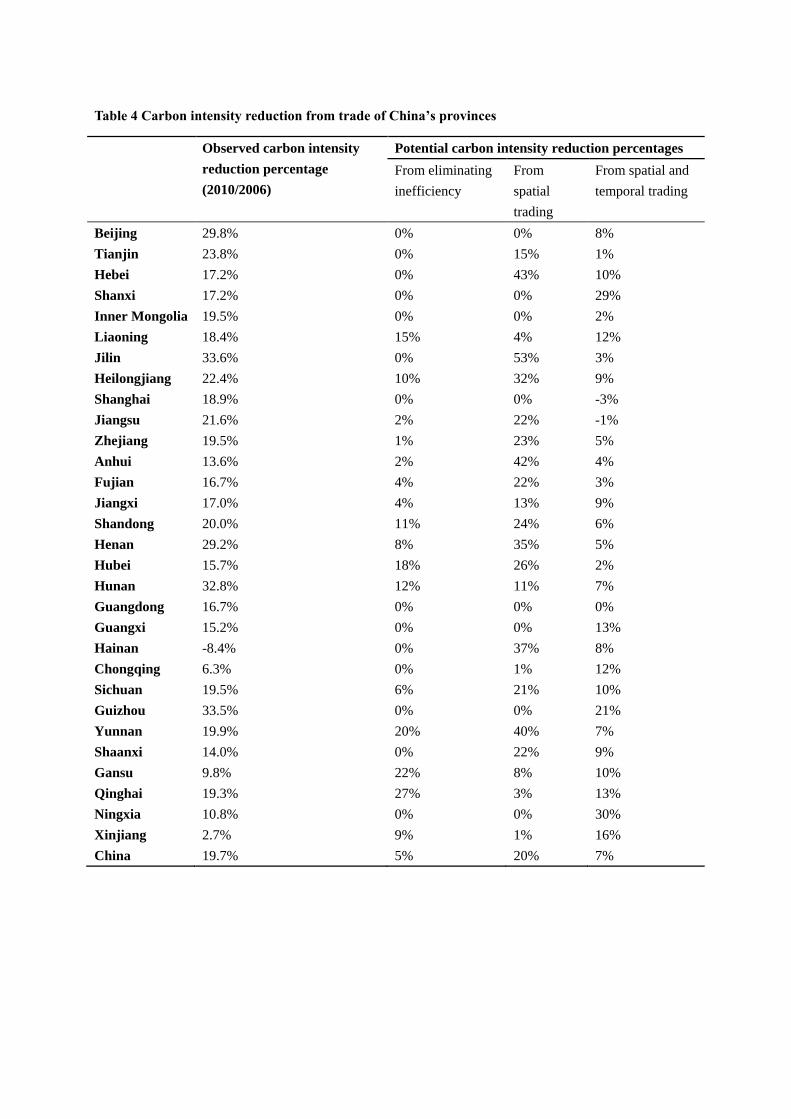
Table 4 Carbon intensity reduction from trade of China’s provinces

Observed carbon intensity

reduction percentage

(2010/2006)

Potential carbon intensity reduction percentages

From eliminating

inefficiency

From

spatial

trading

From spatial and

temporal trading

Beijing 29.8% 0% 0% 8%

Tianjin 23.8% 0% 15% 1%

Hebei 17.2% 0% 43% 10%

Shanxi 17.2% 0% 0% 29%

Inner Mongolia 19.5% 0% 0% 2%

Liaoning 18.4% 15% 4% 12%

Jilin 33.6% 0% 53% 3%

Heilongjiang 22.4% 10% 32% 9%

Shanghai 18.9% 0% 0% -3%

Jiangsu 21.6% 2% 22% -1%

Zhejiang 19.5% 1% 23% 5%

Anhui 13.6% 2% 42% 4%

Fujian 16.7% 4% 22% 3%

Jiangxi 17.0% 4% 13% 9%

Shandong 20.0% 11% 24% 6%

Henan 29.2% 8% 35% 5%

Hubei 15.7% 18% 26% 2%

Hunan 32.8% 12% 11% 7%

Guangdong 16.7% 0% 0% 0%

Guangxi 15.2% 0% 0% 13%

Hainan -8.4% 0% 37% 8%

Chongqing 6.3% 0% 1% 12%

Sichuan 19.5% 6% 21% 10%

Guizhou 33.5% 0% 0% 21%

Yunnan 19.9% 20% 40% 7%

Shaanxi 14.0% 0% 22% 9%

Gansu 9.8% 22% 8% 10%

Qinghai 19.3% 27% 3% 13%

Ningxia 10.8% 0% 0% 30%

Xinjiang 2.7% 9% 1% 16%

China 19.7% 5% 20% 7%

A DEA based estimation on abatement cost savings

Documents

Transcript of A DEA based estimation on abatement cost savings