determination of dynamic properties of nuclear receptors - DEA

THESIS FOR THE DEGREE OF DOCTOR OF PHILOSOPHY (PhD)

Péter Brázda

DETERMINATION OF DYNAMIC PROPERTIES OF NUCLEAR RECEPTORS

Supervisor: Prof. Dr. László Nagy

UNIVERSITY OF DEBRECEN DOCTORAL SCHOOL OF MOLECULAR CELL AND IMMUNE BIOLOGY

Debrecen, 2014

2

Table of Contents

ABBREVIATIONS .............................................................................................................................. 5

INTRODUCTION ............................................................................................................................... 6

TRANSCRIPTION .............................................................................................................................................................. 6 Cells are the functional units of life ........................................................................................................................................... 6 Life is chemistry ................................................................................................................................................................................ 6 Genes are units of biological information .............................................................................................................................. 7 The basic elements of transcription regulation in prokaryotes ................................................................................... 9 Transcriptional regulation in eukaryotes ............................................................................................................................ 11 The chromatin ............................................................................................................................................................................ 11 How do histones influence gene expression? ............................................................................................................... 12 Epigenetics ................................................................................................................................................................................... 13

The initiation of transcription ................................................................................................................................................... 14 What makes transcription initiation gene and signal specific? ............................................................................ 15

THE ‘CLASSICAL WAY’ OF PROMOTER ANALYSIS ............................................................................................... 17 Promoter cloning ............................................................................................................................................................................ 17 EMSA (DNA-‐protein interactions) ........................................................................................................................................... 17 GST-‐pull-‐down (protein-‐protein interactions) .................................................................................................................. 18 Two-‐hybrid system (protein-‐protein interactions) ......................................................................................................... 19

THE NUCLEAR RECEPTORS ........................................................................................................................................ 21 Classes, ligands ................................................................................................................................................................................ 21 The Peroxisome Proliferation Activated Receptors (PPARs) ...................................................................................... 22 The Retinoic Acid Receptors (RARs) ...................................................................................................................................... 23 The Retinoid X Receptors (RXRs) ............................................................................................................................................ 23 Structure ............................................................................................................................................................................................. 24 Coregulators ...................................................................................................................................................................................... 25 Nuclear receptors in action: a model ..................................................................................................................................... 28 The temporal resolution of recent models of NR action ................................................................................................ 28

FLUORESCENCE TECHNIQUES IN CELL BIOLOGY ................................................................................................ 30 Luminescence ................................................................................................................................................................................... 30 The Green Fluorescent Protein ................................................................................................................................................. 31 Fluorescence Recovery After Photobleaching (FRAP) ................................................................................................... 33 Fluorescence Correlation Spectroscopy (FCS) ................................................................................................................... 38 Diffusion models ........................................................................................................................................................................ 39

Adding spatial to temporal: selective plane illumination microscopy – FCS (SPIM-‐FCS) ............................... 41

INVESTIGATION OF TRANSCRIPTION AT THE WHOLE GENOME LEVEL ..................................................... 43 Chromatin immunoprecipitation followed by sequencing (ChIP-‐Seq) ................................................................... 43

HYPOTHESES AND RESEARCH QUESTIONS .......................................................................... 45

Hypotheses ...................................................................................................................................................................... 45

Research questions ...................................................................................................................................................... 45

AIMS ................................................................................................................................................... 46

3

MATERIALS AND METHODS ....................................................................................................... 47 Cell culture and transfection ...................................................................................................................................................... 47 Plasmid constructs ......................................................................................................................................................................... 47 Ligands ................................................................................................................................................................................................ 48 Transient transfection assay ...................................................................................................................................................... 48 Pulsed ligand treatment ............................................................................................................................................................... 48 ChIP (Chromatin immunoprecipitation) .............................................................................................................................. 48 ChIP library preparation for sequencing ........................................................................................................................ 49 ChIP-‐seq data analysis ............................................................................................................................................................ 49

Real-‐time RT-‐PCR ........................................................................................................................................................................... 50 Immunofluorescence detection of RXR in non-‐transfected and stably transfected cells ................................ 50 FCS data acquisition and processing ...................................................................................................................................... 50 Fluorescence correlation spectroscopy (FCS) instrumentation and measurements .................................. 52

Single plane illumination microscopy (SPIM)-‐FCS measurements ........................................................................... 52 SPIM-‐FCS data acquisition and processing .................................................................................................................... 53

Fluorescence recovery after photobleaching (FRAP) ..................................................................................................... 53

RESULTS ........................................................................................................................................... 55

The ‘classical’ promoter analysis of the ABCG2 promoter .............................................................................. 55 PPARγ recognizes the enhancer sequence of the ABCG2 gene ................................................................................... 55 The PPARγ : RXR heterodimer regulates ABCG2 expression by the enhancer element .................................. 56

Nuclear receptors at the single-‐cell level ............................................................................................................. 58 Establishing a GFP-‐based system ............................................................................................................................................. 58 RXR dynamics in live cells as detected by FRAP ............................................................................................................... 62

Dynamics of RXR and RAR at the sub-‐second timescale as detected by live-‐cell FCS ............................ 66 Main characteristics of nuclear RXR and RAR diffusion ................................................................................................ 66 The two-‐component normal diffusion model shows the best fit for RXR and RAR ..................................... 66 Large fraction of RXR and RAR moves around in the nucleus relatively freely ............................................. 70

The effect of ligand activation on receptor mobility ....................................................................................................... 73 Activation shifts the receptors towards a slower state ............................................................................................ 73 The ligand dependent shift in receptor mobility is transient in RXR, unlike in RAR .................................. 76 Coactivator binding is needed for the ligand-‐dependent shift in RAR and RXR mobility ......................... 77 DNA-‐binding determines the steady state of the receptors but has limited effect on the activation-‐dependent changes in mobility ........................................................................................................................................... 85

The mobility map of RXR ............................................................................................................................................ 88 RXR populations show homogenous intranuclear distribution ................................................................................. 88

A global view on the DNA binding of RXR ............................................................................................................. 89 The effect of activation on the number of RXR-‐occupied sites ................................................................................... 90 Agonist treatment increases DNA binding probability of RXR ................................................................................... 95

DISCUSSION ..................................................................................................................................... 96 RXR:PPAR heterodimer binds to a new ABCG2 enhancer element in a ligand dependent manner ........... 96 Live cell microscopy detects the dynamics of RXR activation on the scale of seconds .................................... 97 Fluorescence correlation spectroscopy reveals the effect of DNA and coregulator binding on the dynamic properties of RXR and RAR during activation at the scale of milliseconds ........................................ 97 A refined model of RXR and RAR action, the common features ................................................................................. 98 Differences in the dynamic behaviour of RXR and RAR .............................................................................................. 100 Opening up new dimensions of RXR dynamics I.: SPIM-‐FCS, the diffusion map .............................................. 101 Opening up new dimensions of RXR dynamics II.: ChIP-‐Seq, a glimpse at whole-‐genome scale .............. 101

CONCLUSIONS .............................................................................................................................. 102

4

NEW DISCOVERIES ..................................................................................................................... 103

SUMMARY ..................................................................................................................................... 104

ÖSSZEFOGLALÁS .......................................................................................................................................................... 105

LIST OF KEYWORDS ................................................................................................................... 106

KULCSSZAVAK .............................................................................................................................................................. 106

ACKNOWLEDGEMENTS ............................................................................................................ 107

REFERENCES ................................................................................................................................ 108

PUBLICATIONS ............................................................................................................................ 115 Publications related to the thesis .......................................................................................................................................... 115 Other publications ....................................................................................................................................................................... 116 Oral and poster presentations ............................................................................................................................................... 117

APPENDIX ..................................................................................................................................... 118

ABBREVIATIONS

13-HODE

15-HETE

9cRA

13-hydroxyoctadecadienoic acid

15-hydroxyeicosatetraenoic acid

9-cis retinoic acid

ABCG2 ATP binding cassette sub-family G member 2

ACF autocorrelation function

ACTR nuclear receptor coactivator 3 (Q9Y6Q9)

ATRA all-trans retinoic acid

ChIP chromatin immunoprecipitation

DBD DNA binding domain

DR direct repeat

DRIP vitamin D-interacting protein 205 (Q15648)

ER everted repeat

FCS fluorescence correlation spectroscopy

FRAP fluorescence recovery after photobleaching

FRET Förster's resonance energy transfer

GFP green fluorescent protein (EGFP in our measurements)

H12 helix-12

ID interaction domain

LBD ligand binding domain

NLS nuclear localization signal

NR nuclear receptor

PPAR peroxisome proliferator-activated receptor gamma (P37231)

RAR retinoic acid receptor (P10276)

RE response element

ROI region of interest

RXR retinoid x receptor (P19793)

SMRT nuclear receptor corepressor 2 (Q9Y618)

SPIM selective (single) plane illumination microscopy

TF transcription factor

6

“Essentially, all models are wrong, but some are useful.”

– George Edward Pelham Box

INTRODUCTION

TRANSCRIPTION

Laureate of 2001 Nobel Prize in Physiology or Medicine, Sir Paul Nurse gave a

remarkable talk at the Royal Society where he mentioned the four-plus-one greatest ideas in

the history of biology. This concept was later cited and partially completed by another Nobel

laureate, Roger D. Kornberg. Not surprisingly, the logic and the conclusions of that talk are

far more general than they were presented to be. I will follow the same general notion they

did, but will put emphasis on different points. Most of the fields discussed here have at least

one point in their history, where the technological development was the key to solving a long

unanswered question or to reignite an almost forgotten idea.

Cells are the functional units of life I would set the beginning of the history of the first great idea in biology a bit earlier

than Sir Paul Nurse did. In 1590, when organizing lenses in a tube, a Dutch spectacle-maker,

Zacharias Janssen and his son realized that nearby objects appeared greatly enlarged. Despite

several discrepancies about the real legacy of this invention, it is clear that this was the birth

of the telescope and the microscope. Robert Hooke was the first one to turn the microscope

towards biological objects. The view he saw when investigating a slice of a cork reminded

him to monastery cells that the monks live in, as he mentions in the book Micrographia. Thus

cell biology was born. Anton van Leeuwenhoek, a Dutch tradesman and scientist used his

microscope to have a look at the sample he collected by scratching his teeth. What he saw

were single cell organisms, members of the oral flora. Theodor Scwann phrased the first great

idea of biology in the 1800s stating that all living organisms are composed of cells. These are

the functional units of life.

Life is chemistry As functional units, they carry everything that makes something living. Aristotle

called it ‘vitalism’. The father of modern chemistry, Antoine Lavoisier, revealed what it really

is. Together with Pierre-Simon Laplace they built a calorimeter. By measuring the quantity

7

of carbon dioxide and heat produced by a live guinea pig confined into this apparatus, and by

comparing the amount of heat produced when sufficient carbon was burned in the ice

calorimeter to produce the same amount of carbon dioxide as that which the guinea pig

exhaled, they concluded that respiration was in fact a slow combustion process (1). A

chemical reaction and a physiological process became connected. The second great idea of

biology is seeing life as chemistry. The idea was truly expanded by Louis Pasteur. Apart from

creating the germ theory that experimentally disproves the theory of spontaneous generation,

he studied the processes of fermentation. Mainly these discoveries elevated him to become

one of the fathers of microbiology. The steps of fermentation proceeded mainly inside the

cells, like microscopic fermenters.

Life is chemistry, he said, and now we know that the true effectors of living processes

are proteins, mainly enzymes. These molecules control all the reactions taking place inside a

cell: thousands of reactions, in one single cell, at equal temperature and above all;

simultaneously. Two important features fulfil this seemingly impossible task. One is

compartmentalization. If there is a key characteristic that separates the eukaryotes from the

prokaryotes, it is likely the presence of specialized compartments within the cell. Although

the nucleus is the defining structure, almost all eukaryotic cells also contain a variety of

structures not found in prokaryotes. One or two membranes surround many of these structures.

These compartments allow a variety of environments to exist within a single cell, each with

its own pH and ionic composition, and permit the cell to carry out specific functions more

efficiently than if they were all in the same environment. The second feature is the organized

flow of information.

Genes are units of biological information

Biology can be seen as an original system of processing information. Information

flows into two directions. Horizontally: within one cell or organism and vertically; from

generation to generation. With a clever choice of model organisms, Gregor Mendel laid down

the basis of genetics, though never using the word ‘gene’. He assembled the complicated

appearance of features into the laws of heredity. After his works in the 1860s, nearly thirty

years of silence followed, until they were confirmed and re-discovered. This intermission was

due to the fact that the determined laws were mere theories without any cellular mechanisms

and effectors to bind to. The meeting of biology and microscopy initiated the discovery of

chromosomes by Theodor Boveri (2). Working with nematodes, he and others, including

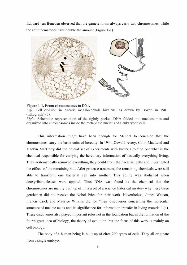
8

Edouard van Beneden observed that the gamete forms always carry two chromosomes, while

the adult nematodes have double the amount (Figure 1-1).

Figure 1-1. From chromosomes to DNA Left: Cell division in Ascaris megalocephala bivalens, as drawn by Boveri in 1901. (lithograph) (3). Right: Schematic representation of the tightly packed DNA folded into nucleosomes and organized into chromosomes inside the metaphase nucleus of a eukaryotic cell.

This information might have been enough for Mendel to conclude that the

chromosomes carry the basic units of heredity. In 1944, Oswald Avery, Colin MacLeod and

Maclyn MacCarty did the crucial set of experiments with bacteria to find out what is the

chemical responsible for carrying the hereditary information of basically everything living.

They systematically removed everything they could from the bacterial cells and investigated

the effects of the remaining bits. After protease treatment, the remaining chemicals were still

able to transform one bacterial cell into another. This ability was abolished when

deoxyribonucleases were applied. Thus DNA was found as the chemical that the

chromosomes are mainly built up of. It is a bit of a science historical mystery why these three

gentlemen did not receive the Nobel Prize for their work. Nevertheless, James Watson,

Francis Crick and Maurice Wilkins did for “their discoveries concerning the molecular

structure of nucleic acids and its significance for information transfer in living material” (4).

These discoveries also played important roles not in the foundation but in the formation of the

fourth great idea of biology, the theory of evolution, but the focus of this work is mainly on

cell biology.

The body of a human being is built up of circa 200 types of cells. They all originate

from a single embryo.

9

What happens in the process of becoming fully differentiated cells?

What is the cause of the difference between the different types of cells?

Do they have the same genetic material at all?

The basic elements of transcription regulation in prokaryotes

Until some crucial experiments, the answer for the latter question was ‘no’. Some part

of the genetic material must get lost during the differentiation, hence making the final results

so different. It was the laureate of the 2012 Nobel Prize for Medicine, Sir John B. Gurdon

who performed these experiments and came up with the concept of differentiation and cell

(re)programming. As it was revealed; our cells own the same sets of genes, having potentially

the same proteome. But they do not. The large DNA molecules in a cell contain specifications

for thousands of proteins. Individual segments of this DNA are transcribed into mRNA,

coding for different proteins. Such segments are called genes. Instead of manufacturing the

whole repertoire at full tilt all the time, the expression of individual genes is regulated

according to the cell’s needs. Pieces of regulatory DNA are interspersed among the segments

that code for protein. These noncoding sequences can bind special molecules that affect the

expression of their regulated genes (5).

The DNA acts as a digital information-storage device. The cell with all its components

is like the hardware, built up of information networks, hubs, elements for effector and quality

control processes. In cell biology the term ‘wetware’ might bring us closer to reality as the

information flows in forms of small molecules in the cyto- or nucleoplasm and it is read and

executed by proteins. Information is from one side arriving from the outer- or inner

environment of the cell. These are impacts that need to be answered. The toolbox is given but

the potential response has to be chosen and carried out. Additionally to giving out the orders

for action, the process needs feedback control. That is the only way to fine-tune the response.

In the chromosome of the bacterium E. coli, that is a single circular DNA, many genes

are arranged into clusters. They are not just positioned adjacent to each other but are under the

control of one single promoter and are transcribed as one single strand of mRNA (5). This

cluster is called the operon and was described by Jaques Monod. The genes of one operon

usually encode proteins for one metabolic pathway thus the common regulation.

Many aspects are different in the eukaryotic transcription regulation, but the main

features are the same; the regulation is carried out by repressors and activators and controlled

via feedback mechanisms. A promoter is a specific DNA sequence, a motif that is recognized

by the RNA polymerase. As it binds to the DNA and unwinds the double helix, mRNA

10

synthesis can start according to the opened up DNA-template. There is one way to interfere

into this process, when inhibition is needed. There is a regulatory motif between the promoter

sequence and gene body. A repressor protein recognizes this sequence. When there is enough

tryptophan around the E. coli, there is no need to synthetize any. The tryptophan repressor can

bind the intracellular tryptophan that keeps the protein in active conformation. In this state it

is able to bind to its recognition sequence that is located right in front of the gene coding the

enzymes of tryptophan synthesis and in the close proximity of the promoter. As the repressor

is bound to the DNA, it blocks the binding of the RNA polymerase, thus inhibiting the

expression. As the level of tryptophan drops and it is not available for the repressor, it is

converted into its inactive formation that cannot bind to DNA, liberating the genes of amino

acid synthesis from the repression.

Figure 1-2. Regulation of the lac-operon by a pair of repressor and activator. (6)

In some cases positive regulation is needed, when the expression of a gene is only

necessary under certain circumstances. Most bacterial promoters are recognized poorly by the

RNA polymerase. Some parts of the double helix are too hard for the polymerase to open. In

such cases there is no transcription going on. On the lac-operon that codes the enzymes for

carbohydrate metabolism, apart from repressors, activators are present as well (Figure 1-2).

The catabolite activator protein (CAP) can bind cAMP, the general hunger-signal, when the

glucose level drops in the medium of the bacterium. In this active form, the CAP can bind to

its binding site near the promoter of the operon. As a result of activator binding, the double

helix is loosened up via direct interaction between the CAP and the polymerase; the latter has

11

an increased affinity and thus higher probability to bind to the promoter. What follows is the

transcription of the enzymes that import and process lactose, as a plan B instead of glucose.

Transcriptional regulation in eukaryotes

The chromatin

The appearance of the eukaryotic cell brought important changes both in the size and

the organization of the genome. The genome size (C-value) of an organism bears no

relationship with its complexity (7). The C-value enigma has several possible explanations

and was resolved by the discovery that the genome of an eukaryotic cell contains not only

functional genes but also large amounts of sequences that do not code proteins (introns,

pseudogenes, spacer and repetitive sequences)(8). The human genome is thought to contain

approximately 100,000 genes (only about 25 times more than the E. coli).

The length of the haploid DNA-content of a human cell is longer than 1 metre. This

staggering amount of genetic material is packed into the absurdly small volume of a cell

nucleus sized roughly 10 micrometres in diameter. The task is not just to cram the DNA into a

depot but also to pack it so that it is still available for replication and transcription. It has to be

available to fulfill a highly dynamic and precise regulation. To some extent the tight packing

of the genome also serves protective aims preventing DNA break.

This packed form of the genome is the chromatin. It is a collection of DNA and

protein. The basic structural unit of the chromatin is the nucleosome. Roger Kornberg

proposed this model in 1974 after a set of well-focused experiments. Two sets of micrococcal

nuclease (an enzyme for not sequence specific DNA degradation) digestion experiments were

done. The sample that contained every element of the chromatin (DNA + protein) yielded

DNA fragments that were about 200 base pairs long. In contrast, the sample that lacked the

protein content (naked DNA) yielded randomly sized fragments (a distinctive smear when

investigated by electrophoresis). He concluded that the enzyme could attack DNA only at

sites separated by approximately 200 base pairs. These units of the chromatin are built up of

histone proteins. They form the core of the beads that the string of DNA is laced around. The

core histones are the H2A, H2B, H3 and H4. The DNA strand takes 1.65 turns around the

octamer formed by the core histones making a contact via 166 of its base pairs. There is a

strong ionic interaction between the basic histone proteins and the negatively charged DNA.

This makes the region of the genome that is packed into nucleosomes hard to reach for any

other protein (Figure 1-3). As seen the H1 is missing from the list, as this is a linker histone,

binding the DNA at the nucleosome entry site, holding the structure in place. AT-rich

12

sequence motifs are generally the more flexible regions of the genome. This flexibility of the

DNA strand is important for the building up of the nucleosomal structure. So the DNA

sequence can influence the localization of the nucleosomes on one hand. On the other hand

this is a statistical influence as a short, 10 base pair long motif is already giving a curved

DNA that is more prone to give a perfect site for the nucleosome. This marks large regions

along the DNA that can form nucleosomes, so the final localization of the complex is

influenced by other factors as well.

Figure 1-3. The nucleosome structure.

How do histones influence gene expression?

In 1928 the German botanist Emil Heitz visualized in moss nuclei chromosomal

regions with different states of condensation (9). He was the first to use the expression

heterochromatin for the condensed regions, whereas fractions of the chromosome that were

decondensed and spread out diffusely in the interphase nucleus he called euchromatin. He

hypothesized the euchromatin parts being ‘genetically more important’. Edgar and Ellen

Stedman found that histones could be general repressors (10) and as they are linked with the

heterochromatin, the ‘default OFF’ state appeared to be the general concept in eukaryotic

gene regulation as opposed to the prokaryotic ‘default ON’ state. It is a logical assumption

from these ideas that the removal of histones is required for gene activation in the nucleus.

13

After an interesting set of experiments, Paul and Gilmour (11) concluded: when

purified mammalian DNA is recombined with histone proteins in the presence of a non-

histone fraction from chromatin, this reconstituted nucleoprotein exhibits the same template

activity as the original chromatin. Histones can mask DNA in chromatin and prevent it from

acting as a template, but this effect is nonspecific. Other non-histone molecules are

responsible for unmasking organ-specific DNA sequences. So, the genome dictates not only

the nature of the cell’s proteins, but also when and where they are to be made. The tools for

this regulation are the transcription factors. The organization and structure of the given

genetic material and the set of available transcription factors are the key determinants of a

cell’s fate as far as its differentiation, and response to the outer and inner environment is

concerned.

Epigenetics

The terminal regions of histone proteins, the so-called histone tails, are subject to

several covalent post-translational modifications. On the N-terminal acetylation, methylation,

phosphorylation and ribosylation, on the C-terminal ubiquitination can take place (12) (Figure

1-4). By the eighties it was clear that enzymatic modification of histone tails was essential for

transcription regulation. These modifications can be added and removed by chromatin

modifying enzymes. Epigenetic regulation is based on remodelling of chromatin structure.

Histones and their modifications are key parts of the epigenetic machinery. These tags act as

cellular memory; it is the propagation of cell regulatory states from mother cell to daughter

cell. This is crucial for a multicellular organism as the distinct functional identities of the cells

of different organs need to be kept up despite their identical genomes and often similar

environment. At the same time adaptive flexibility is also desired. The enzymes carrying out

the modification are themselves part of the regulation that makes the transcription machinery

a full circle.

14

Figure 1-4. Potential post-translational modifications of histone tails

Lysine and arginine residues both contain amino groups, which confer basic and

hydrophobic characteristics. Lysine is able to be mono-, di-, or trimethylated. Generally,

methylation of an arginine residue requires a complex including protein arginine

methyltransferase (PRMT) while lysine requires a specific histone methyltransferase (HMT)

(13). Common sites of methylation associated with gene activation include H3K4 (lysine 4 of

histone 3), H3K48, and H3K79. Common sites for gene inactivation include H3K9 and

H3K27. Euchromatin is characterized by a high level of histone acetylation, which is

mediated by histone acetyl transferases (HATs). Lysine acetylation partially removes the

charges of the histone tail, making them more hydrophobic. This in turn weakens the DNA-

histone interaction. At the same time, these residues are more important in interactions

between the nucleosome and non-histone proteins. Conversely, histone deacetylases

(HDACs) have the ability to remove this epigenetic tag, which leads to transcriptional

repression.

The organization of acetylated and methylated residues gives a distinct pattern for the

given genomic region. This histone code influences the composition of the protein complexes

recruited.

The initiation of transcription

The DNA polymerase II (PolII) is responsible for the transcription of mRNA in

eukaryotes, so I will now focus on the initiation of this type of transcription. Unlike its

bacterial form, eukaryotic PolII is not responsible for sequence recognition. Also, it can only

catalyse and not initiate transcription.

15

What are the other factors that help the PolII in targeting?

The basal transcription machinery is built up of the polymerase itself and the basal

factors. TFIID is a 800 kD complex. TBP (TATA-binding protein) is its largest subunit that

recognises the TATA-box at the core promoter. This sequence is located 25 bp upstream the

transcription start site. The TA-rich region is nested by GC-rich sequences. It is interesting

that nucleosomes also favour the TA-rich regions. This competition between the nucleosomes

and the basal transcription complex is an additional feature showing how the events of

transcription initiation are linked. As TBP binds to the minor groove of the DNA at the

TATA-box, the region is pinned. A chain of events follows this step.

TAFs (TBP-associated factors) form the other subunit of TFIID. They appear in

several, mainly tissue-specific forms. TAFs can form interactions with other complexes

giving (tissue and signal) specificity to the initiation. The binding of TFIID is followed by the

TFIIA and TFIIB that clearly localizes the initiating events to the affected region. The TFIIF

complex is the next key element in the process. It brings ATP-dependent DNA-helicase

activity into the events and melts the DNA double helix. This complex is also able to form

direct interaction with the PolII.

So, it is all set: the site of initiation is free of nucleosomes, the TATA-box was

available for the TFIID, which recognized the sequence and helped the basic transcription

machinery to build up at the start site. The starting pistol is the TFIIH. It harbours ATPase and

kinase activity. Phosphorylation of PolII makes it possible to escape from the initiation site

and run into transcription.

What makes transcription initiation gene and signal specific?

The TBP recognizes a short and simple TATA motif on the DNA and the PolII has no

sequence specificity. What directs these low-specificity binding events to the right position?

The TATA-box with the promoter is only enough for a low efficiency and low specificity

transcription initiation. Sequences with specific motifs, hundreds of base pairs away from the

promoter, called enhancers and the DNA-binding proteins that recognize these regions, called

activators largely increase the specificity and efficiency of transcription initiation. Enhancers

can be localized both up- and downstream form the promoter. Even in comparison with the

promoter, these regions recruit large protein complexes. These enhancosomes are cell-type

and signal specific. In most cases every member of the complex is needed for the total activity.

The transcription factors that bind to these sequences are the activators and the highly specific

sequences these proteins recognize are the response elements (RE). The proteins in the focus

16

of this thesis belong to this group. They are nuclear receptors with a complex role that is

mirrored on the types of interactions they can take part in: DNA-protein interaction via

specific recognition sites, ligand-protein interactions by binding different molecules of

signaling mechanisms, protein-protein interactions by making contacts with further members

of the regulatory complex.

The gap between the basal transcription machinery (including PolII itself) at the

promoter and the activators at the enhancer site is bridged by coactivator proteins.

Coactivators harbour multiple docking sites for further members of the activator complex.

The function of coregulator proteins will be discussed later in relation with the molecular

switch model of transcription regulation. An other important feature of these molecules is the

histone acetyltransferase (HAT) activity. At this point the positioning of nucleosomes, the

signal-specific modification of histone tails, the cell-type specific coactivator repertoire and

the initiation of transcription meets.

Exploring the position and functions of genomic regions that can serve for specific or

unspecific docking sites for proteins of expression regulation and the composition of

regulatory complexes are understandably of key importance. The methods applied for this

task has changed a lot and usually reflect the actual trends of molecular biology.

THE ‘CLASSICAL WAY’ OF PROMOTER ANALYSIS

Promoter cloning

The journey starts when a new gene is cloned. It is fundamental to clarify the type of

regulation that influences the expression of this gene. First the promoter of the new gene has

to be found. When the cDNA has been isolated and characterized, it is possible to use this

cDNA as a probe to screen a genomic library and to isolate the corresponding gene. After

screening of different tissue cDNA libraries, a gene can be cloned. Then in vitro translation of

this clone gives a polypeptide that can be investigated for its identity with antibodies. The

deduced amino-acid sequence and the nucleotide sequences can be used for homology studies

(14). The objective of the following promoter analysis is to understand what cis-acting DNA

sequences are responsible for the regulation of the gene’s expression. Cis-acting sequences

are regulatory sequences that are part of the gene whose expression is being studied. Although

these sequences are most frequently found just upstream of the transcription start site (TSS),

they can also be found further upstream, or on the 3' of the gene, or even within the introns

and exons. To fully understand how these sequences operate it is necessary to understand the

protein complexes that interact with these elements.

Once a suspected regulatory region is found, it can be tested by the transient

transfection of a reporter system. The region is spliced up, or narrowed down if a minimum-

promoter is to be identified and cloned in front of a reporter gene in a plasmid vector. The

most common reporters are the luciferase and the chloramphenicol acetyltransferase (CAT).

During the test, the reporter is under the effect of the investigated regulatory element. The rate

of enzymatic activity of the reporter protein is in correlation with its level of expression that

in turn reflects the regulatory effect of the cloned sequence. Modifying the original sequence

and investigating the consequences is one way to follow such study. Clearly, there are

limitations on the size of the regions that can be scanned by this method.

EMSA (DNA-‐protein interactions)

The next step in solving a cistrome is to identify the proteins that bind directly or

indirectly forming the regulatory complexes. This is usually done by electrophoretic mobility

shift assay (EMSA), which is a method for the in vitro detection of DNA-protein interactions.

The oligonucleotide that is the suspected recognition sequence of the DNA-binding protein

has a label on it that is most commonly a radioactive tag. The in vitro translated protein (with

or without its binding partners) is then mixed with the radio-oligonucleotides and loaded to a

18

polyacrylamide gel. The speed at which different molecules move through the gel is

determined by their size and charge (and to a lesser extent, their shape). The control lane

(radio-oligonucleotide without protein) will contain a single band corresponding to the

unbound DNA fragment. However, assuming that the protein is capable of binding to the

fragment, the lane with protein present will contain another band that represents the larger,

less mobile complex of nucleic acid probe bound to protein, which is “shifted up” on the gel

(it was moving slower). Altering the binding sequence or the partner proteins can give a

deeper understanding about that DNA-protein interaction (Figure 1-4).

Figure 1-4. Overview of the EMSA method. After Thermo Scientific

GST-‐pull-‐down (protein-‐protein interactions) At this point the promoter region is known. But it has already been discussed that the

specificity and the efficiency of the transcription initiation is based on the regulatory

complexes, in other words; on protein-protein interactions.

GST-pull-down is among the most widely used methods in molecular biology. The

core of this method is a bait protein bound to a solid surface (via its GST-tag) and mixed with

the in vitro translated (and radiolabelled) potential partner. When interaction happens, the

formation of the complex can be detected on a gel (SDS-PAGE). The different partners and

the regulating effects (activation) can be detected by this method in a cell-free environment.

19

Two-‐hybrid system (protein-‐protein interactions)

Another method to determine protein-protein interactions is the two-hybrid system

(THS). It was originally worked out in yeasts, but the essence of the method is mainly the

same when it is being applied in mammalian cells. It is important to point out that

theoretically, it can be used to detect interactions between any types of proteins. It is also

based on the fishing-out concept; a bait-protein is fused to yeast DNA-binging domain (GAL-

bait) and the prey protein is fused to a viral transcription transactivation domain (prey-VP).

The reporter plasmid codes for a protein that is not expressed endogenously in a mammalian

cell (Luciferase), and a regulatory region upstream to it, that is recognized only by the GAL-

domain. The elements of the system are coded on plasmids. By transient transfection they can

act inside a mammalian cell, using it as an incubator and letting all the endogenous proteins

(endogenous coregulators, polymerases, etc.) act, making it a cell-based method (15).

Figure 1-5. The basis of the mammalian two-hybrid system. (16)

All the plasmids (coding for GAL-bait, prey-VP, UAS-Luciferase) are transiently

transfected into the cells. The bait and prey proteins are expressed freely. When they interact

and form dimers, they make up a ‘proper’ transcription factor; the dimer binds to the DNA

(UAS-site) via its GAL-domain and enhances the transcription of the downstream gene

(Luciferase) by its VP-domain. The rate of enzymatic activity of the reporter protein is in

correlation with its level of expression that in turn reflects the strength of the bait:prey

interaction (Figure 1-5).

By the application of these and other, related methods cellular mechanisms can be

mapped in a reductionist manner. Generally, interactions of two or some molecules are being

investigated at a time and their complex relationship is mapped according to these data. The

20

molecules of interest have to be in a form that enables them for being investigated. This might

include the lysis of the cell, recovering, extracting and perhaps cross-linking the proteins.

Recent advances of molecular biology, imaging and fluidic techniques made it possible to

investigate cellular mechanisms in a ‘minimal invasive’ fashion.

THE NUCLEAR RECEPTORS

Some transcription factors are synthesized only in specific tissues. The activities of the

factors themselves are also regulated in different cell types. Regulatory signal that activates

eukaryotic transcription factors can originate from a very distant source in the body. For

instance, hormones released into the circulatory system by an organ that is part of the

endocrine system travel through the circulation to essentially all parts of the body. The

endocrine system can thus serve as a regulator to coordinate changes in transcription in cells

of many different tissues. Some hormones are small molecules that, because of their lipid-

solubility properties, can directly pass through the plasma membrane of the cell –like steroid

hormones, such as glucocorticoid, testosterone, and estrogen. In the cell, steroid hormones

bind to and regulate specific transcription factors in the nucleus. (17) In metazoans they are

called nuclear receptors (NRs).

Classes, ligands

Nuclear receptors have long been in the focus of attention for many scientific projects

aiming to explain the mechanism of the genetic information’s flow. They are located in the

cytoplasm or in the nucleus and are activated by small lipophilic molecules that can be

originated from outside or inside the cell. One way of NR classification is based on the

characteristics and source of their ligands (Table 1-1). For steroid hormone receptors the

ligands are synthesized exclusively in endocrine organs. These receptors are mainly

cytoplasmic. In the unliganded (apo) form they are bound to heat-shock proteins and thus held

back in the cytoplasm. As the agonist ligand arrives after diffusion through the plasma

membrane, the heat-shock proteins are released and the NRs translocate to the nucleus to bind

to activator complexes and induce the transcription of their target genes (18). Receptors of

this group include the estrogen receptor (ER), the androgen receptor (AR) or the

glucocorticoid receptor (GR). Non-steroid hormone receptors recognize ligands derived from

dietary lipids (vitamin A, cholesterol) or require exogenous elements for their synthesis

(vitamin D, thyroid hormone). Members of this group, like the retinoic acid receptor (RAR),

the thyroid hormone receptor (TR) or the vitamin D receptor (VDR) localize in the nucleus

(19). As such, they are prone to bind to repressor complexes and thus act as repressors in

absence of ligand. In the ligand-bound (holo) form they show an increased affinity to the

activator complexes, as it will be described in the ‘molecular switch model’ later. The third

group includes the orphan receptors that have no characterized ligand or target gene.

According to a hypothesis, the ancestral NR was an orphan activator or repressor and gained

22

ligand binding ability during evolution. The fourth group includes the adopted orphan

receptors. The adoption process involves the recognition of a physiological ligand for the

receptor. These are usually low-affinity ligand-receptor interactions. Dietary lipids, the

ligands of these receptors, are present at low physiological concentrations. Members of this

group are the retinoid x receptor (RXR), the peroxisome proliferation activated receptor

(PPAR) or the liver x receptor (LXR) (20).

Endocrine Receptors Adopted Orphan Receptors

Orphan Receptors

Ligands with high-affinity, hormonal lipids

Ligands with low-affinity, dietary lipids

Unknown ligands

Estrogen Receptor (ER) Retinoic X Receptor (RXR) RAR-related Orphan Receptor

(ROR) Androgen Receptor (AR) Peroxisome Proliferator

Activated Receptor (PPAR) Hepatocyte Nuclear Factor

(HNF4) Glucocorticoid Receptor

(GR) Liver X Receptor (LXR)

Retinoic Acid Receptor (RAR)

Thyroid Hormone Receptor (TR)

Table 1-1. Groups of nuclear receptors based on the nature of their ligands Table is based on figure taken from (20).

The Peroxisome Proliferation Activated Receptors (PPARs) The unorthodox name of these receptors stands as a reminder of the initial cloning of

one isoform as a target of various xenobiotic compounds that were observed to induce

proliferation of peroxisomes in the liver (21). That isoform was the PPARα. Soon the

discovery of PPARδ and PPARγ came (22, 23). Many cell types express more than one PPAR

isoform, which raises the question of how isoform-specific targets are regulated. Most likely

this occurs through a combination of subtle cis-sequence differences flanking the core RE, the

presence of specific or selective coactivator proteins, and regulation of endogenous ligands

(24).

A variety of fatty acids and their derivatives have been found to bind to PPARγ with

relatively low affinity. Eicosanoids, such as 13-HODE and 15-HETE, have also been

suggested to act as PPARγ ligands (25). Several high affinity synthetic PPARγ ligands have

been generated. These include the thiazolidinedione (TZD) class of drugs, which are used

clinically as insulin sensitizers in patients with type-two diabetes.

23

They bind to DNA with the obligate heterodimer partner, the RXR. PPARs recognize

the consensus PPRE half-site of a DR1 motif.

The Retinoic Acid Receptors (RARs) The nuclear protein called RAR binds retinoic acid, the biologically active form of

vitamin A. Unlike members of the other protein superfamily, the steroid receptors, retinoid

receptors are constantly localized in the nucleus. RARs are reported to be bound to their RE

and act as repressors in the absence of agonist ligand. They show high affinity for the RXR

that is their obligate dimeric partner, just like for the PPAR. Their endogenous ligands are the

all-trans retinoic acid (ATRA) and the 9-cis retinoic acid. Interestingly, the latter one can bind

to the RXR as well. This phenomenon also shows the intimate and unique relationship

between these two receptors.

The Retinoid X Receptors (RXRs)

After the identification of the receptors for all-trans retinoic acid another receptor was

discovered that was capable of mediating retinoid-signalling pathways (26). Parallelly, a new

cofactor was reported that appeared to be necessary for the RAR to bind to its RE (27). These

reports were pointing at a new nuclear receptor, the RXR. The strong homology of the three

isoforms (α,β,γ) indicates that they regulate common targets by binding similar ligands and

recognizing similar sites. The difference is in their topological pattern of expression. RXRα

and RXRβ are expressed in a wide range of tissues like kidney, spleen, placenta and epidermis.

RXRγ is, in contrast mainly expressed in muscle and brain tissues (28).

Several molecules have been described as potential RXR ligands like 9-cis RA (29),

docosahexaenoic acid (30) or synthesized as selective ligands like LG100268 (31). Still, the

endogenous ligand for RXR has not been found yet.

RXRs are unparalleled in a sense that they can form heterodimers with at least twenty

other nuclear receptors. ATRA, the ligand for RAR does not bind to or activate RXR. At the

same time, 9-cis retinoic acid does (29). To distinguish the group of molecules that attribute

their biological activities to interaction with RXR from the ones that do with RAR, rexinoids

and retinoids are distinguished, respectively (32).

Based on their activation pattern in the mammalian two-hybrid studies RXR-

heterodimers are divided into two groups. In a non-permissive heterodimer the partner (like

RAR) actively interferes with the ability of RXR to activate transcription in response to RXR-

24

specific ligands. The dimer cannot be activated selectively from the RXR side. Activation

from both sides of the dimer has a synergistic effect on transactivation. In contrast, permissive

heterodimers allow RXR signalling and act as bi-functional transcription factors. RXR forms

permissive heterodimer with PPAR (33).

Structure

This superfamily of proteins consists of transcription factors that harbour many key

elements of transcriptional regulation in one single molecule. Due to their structure they offer

surfaces for numerous types of interactions thus multiplying the number of available levels of

regulation.

Figure 1-6. The general structure of a nuclear receptor Left: Chrystal structure of the PPARγ ligand binding domain (LBD) and the RARa DNA-binding domain (DBD) with the response element. The two parts of the protein were manually constructed next to each other. Right: Schematic representation of the parts of the nuclear receptor. AF2, AF1- activating functions, LBD – ligand binding domain, D – hinge domain, DBD – DNA binding domain

Most importantly, via the DNA-binding domain (DBD), nuclear receptors can directly

bind to DNA (Figure 1-6). High affinity binding is made possible by the two zinc finger

motifs. This domain recognizes the specific hormone response elements (RE) (34). REs are

sequence motifs that are mainly located close to the promoter, but more and more genes are

revealed that has enhancer regions with binding sites located several kilobases upstream the

TSS. A consensus RE sequence is AGGTCA (35), which acts as a half-site. The receptors

bind to two, neighbouring half-sites as dimers. The relation and the position of the two half-

sites determine the potentially binding dimers. Non-steroid nuclear receptors (RXR, RAR,

PPAR, VDR or LXR) typically recognize direct repeats (DR). The number of nucleotides

25

separating these half-sites selects between the dimers. DR1 (AGGTCAnAGGTCA) for the

PPAR:RXR, DR2 for the RAR:RXR, DR3 for the VDR:RXR, DR4 for the LXR:RXR and

DR5 for the RAR: RXR. The central role of RXR as a dimer partner can clearly be seen from

this list.

A hinge region that gives a high degree of flexibility for the overall structure follows

this well conserved N-terminal domain. This section harbours the nuclear localization signal

(NLS) as well.

Dimer formation is partially linked to the DBD, but it mainly happens through the

ligand-binding domain (LBD). The core of nuclear receptor action lies in this domain. Its 12-

helical structure appears to be conserved between different species. The C-terminal helix

(H12) is the most notable one. The sequence of this domain is highly conserved among many

NRs. Its role in NR action will be discussed later.

A ligand-binding pocket is formed in this domain with variable volume and lining of

residuals that are responsible for the specific binding of ligands (36). As ligand binding

happens, structural changes take place in the protein, changing its repertoire of available

binding surfaces and thus the affinities of the nuclear receptors for other proteins.

This leads us to the third type of interactions that NRs are able to form (apart from

protein-DNA and protein-ligand interactions). Combinational regulation by NRs is mostly the

result of various response elements that are differentially available, due to the epigenetic

landscape of the cell. The combinational level is further increased, when we bring protein-

protein interactions into the picture. The LBD is the surface for the dimer formation as well.

Some NRs can act as monomers, but most of them form homo- or heterodimers. In this

respect, as it was mentioned earlier, the retinoid-x receptor is a key molecule in this system,

as it acts as a promiscuous partner being able to form heterodimers with several other types of

NRs, including the RAR, the PPAR, the VDR, or the LXR. The above-mentioned ligand-

induced conformational change affects mainly the other kind of protein-protein interaction

taking place on the LBD. Coregulators are cooperative proteins for the NR action.

Coregulators

Acetylation of histone residues strongly correlates with transcription status. It is

mainly determined by the enzymatic activities of histone deacetylases (HDACs) and histone

acetylases (HATs). These modifications can be directed by their interactions with NRs

forming a bridge towards the other members of the transcription machinery. Coregulators act

as mediators for the NRs. The two kinds of coregulators; corepressors and coactivators are

26

found to bind to the same region of the receptor. Coactivators mediate the interactions of

transcription factors with the basal transcriptional machinery (37). Members of the p160

protein superfamily, such as ACTR/SRC-3 show 40% sequence homology. By definition they

form ligand dependent interactions with NRs, which means there is no binding between the

coregulators and the apo-receptors. They act as real docking sites for the building up of large

multiprotein complexes. Different domains of the coactivators can interact with an arginine

methyltransferase, with CREB (cAMP response element binding protein) binding protein and

via their two LxxLL motifs, called interaction domains (ID) they can bind to NRs.

Coactivator possess HAT activity that is crucial for the signal-integrating function and for

translating the activating signal to chromatin-remodeling action. DRIP205 is also a member

of a large coactivator unit (Figure 1-7).

On the other hand, unliganded TR and RAR was found to interact with certain

proteins in biochemical assays. One of those proteins was the previously identified silencing

mediator for retinoid and thyroid hormone receptors (SMRT). In a reporter system the

interaction resulted in a strong repression of the basal transcription machinery, but it was

ligand reversible. Analogous to coactivators, corepressors also harbour two LxxLL-related

motifs called the CoRNR-boxes. The striking similarity of the amphipathic conformation of

the IDs of coregulators suggests that they may bind to similar or overlapping surfaces of the

NR.

27

Figure 1-7. Protein-protein interaction in NR action Above: Coactivator and corepressor involved in nuclear receptor-mediated transcriptional regulation. Under: The ‘molecular switch’ model of NR action (38)

28

Nuclear receptors in action: a model The above-mentioned, mainly biochemical methods were the keys to a working model

of NR action, the ‘molecular switch model’. According to this concept, in the absence of

ligand corepressors and further members of the repressor complex, including HDACs are

bound to the NR. This favours for the formation of condensed nucleosomal structure. The

latter restricts transcription factors access to the chromatin, resulting in a repressed state of

transcription in that genomic region. As the agonist ligand appears and binds to the pocket of

the LBD, conformation changes take place (39). Great amount of mutational, activity and

structural studies were carried out with retinoic acid receptors, and others, revealing the

working mechanism of the switch. The agonist-dependent repositioning of helix-12 (holo-

form) causes a shift in the affinities between different coregulators and the NR. The holo-

form has decreased ability to bind to the corepressors, but an increased affinity for the

coactivators, such as ACTR (ACtivator for Thyroid hormone and Retinoid receptors) or

DRIP/TRAP. In a cellular environment these sum up in the exchange of coregulators bound to

the LBDs of the dimer. As a result of the coactivator binding, new sets of proteins are being

recruited as members of the activator complex, including HATs. By creating an acetylated

milieu in that genomic region via the histone-tail modifications, the change of coregulators

ends up in transcriptional activation.

The temporal resolution of recent models of NR action

The operon model and also the molecular switch model describe binary systems. The

pathway is either turned on or off. It is a yes-or-no situation. Adding dynamics to the

description of cellular processes is like moving from a binary code to the Morse coded

sonnets of Shakespeare.

Due to the ever increasing number of identified coregulators, and the several

complexes they can be associated with, it has become evident by now that there must be some

functional redundancy and a greater flexibility in coregulator-receptor interactions. The

potential of combinatorial regulation, the high 3D flexibility of receptors and the determining

role of local nuclear architecture are all pointing towards the formulation of a more flexible

and dynamic model. Most importantly the contribution of diffusion and mobility in the

nucleus has not been accounted for in most of the models proposed, which have been largely

based on transfection and biochemical analyses as well as protein structures (40).

29

Chromatin immunoprecipitation (ChIP) revealed a new feature of transcription factors.

The alteration of unproductive cycles marked by rapid DNA binding and ligand-dependent

productive cycles with reduced mobility and longer binding-times seems to be the essence of

estrogen receptor (ER) action. Based on the cyclic binding of ER, HDACs and PolII, the new

model has pointed towards a highly integrated transcriptional ratchet (41) that ensures

dynamic and controlled response to stimuli, but requires elements being highly mobile. Cross-

linking, fixation or lysis based and cell free biochemical methods are of great use when the

aim is to investigate isolated elements and actions of the system. One great drawback of these

systems is that they are usually cell free and thus the interactions are taking place outside their

actual environment. The other one is the lack of real time resolution. As the dynamic nature

of transcription regulation started to shine through the results of experiments taken at different

time points, a new era of cell and molecular biology started to gain importance (Figure 1-8).

Figure 1-8. Cyclical recruitment of transcription factors to the pS2 promoter. The periodic association of HATs, HDACs, HMTs and SWI/SNF (Brg/Brm), as well as other important complexes that contribute to ER dynamics and promoter clearance are shown with arrows. The association phase of each productive cycle is shown by grey bars. Specific recruitment of NuRD at the end of the second transcriptionally productive cycle corresponds to NucT remodelling, displacement of TBP and demethylation of dimethylated histone H4 R3. Ac-H3 - acetylated histone 3, Ac-H4 - acetylated histone 4, APIS - AAA ATPase proteins independent of 20S, ERE - estrogen response element, HAT -histone acetyltransferase, HDAC - histone deacetylase; HMT - histone methyltransferase, Met-H3 - dimethylated histone 3, Met-H4 - dimethylated histone 4, NucE - nucleosome including the ERE, NucT - nucleosome including the TATA box, NuRD - nucleosome remodelling and deacetylating complex, p68 - p68 RNA helicase, TBP - TATA-binding protein. Figure taken from (41).

FLUORESCENCE TECHNIQUES IN CELL BIOLOGY

Luminescence Luminescence is the emission of light from any substance. It occurs from

electronically excited states (42). Photoluminescence describes the light emission after the

absorption of photons as electromagnetic radiation. The two usually distinguished forms of

photoluminescence are phosphorescence and fluorescence. Phosphorescence is emission of

light from (triplet) excited states, in which the electron in the excited orbital has the same spin

orientation as the ground-state electron. Transitions to the ground state are forbidden and the

emission rates are slow, so that phosphorescence lifetimes are typically milliseconds to

seconds. Following exposure to light, the phosphorescence substances glow for several

minutes while the excited phosphors slowly return to the ground state (as in case of glowing

toys).

Fluorescence typically occurs from aromatic molecules. By illuminating quinine

sulphate with different wavelengths using a prism, and the sun as a light source George

Gabriel Stokes recognized that the emitted fluorescence has a longer wavelength than

the incident light. The ultraviolet light from the sun excites the quinine in tonic water. Upon

return to the ground state the quinine emits blue light with a wavelength near 450 nm.

An important feature of fluorescence is high sensitivity detection. The sensitivity of

fluorescence was used in 1877 to demonstrate that underground streams connected the rivers

Danube and Rhine. This connection was demonstrated by placing fluorescein into the Danube.

Some sixty hours later its characteristic green fluorescence appeared in a small river that led

to the Rhine (43).

The Jablonski diagram, named after Alexander Jablonski, illustrates the processes that

occur between the absorption and emission of light. The states are drawn vertically by energy

and grouped horizontally by spin multiplicity. Waved arrows indicate nonradiative transitions

and straight arrows indicate radiative transitions (Figure 1-9). The singlet ground, first, and

second electronic states are labelled S0, S1, and S2. Within these electronic energy levels the

fluorophores can exist in different vibrational energy levels: 0, 1, 2. The transitions between

states are depicted as vertical lines. Transitions occur in about 10–15 s. Absorption and

emission occur mostly from molecules with the lowest vibrational energy. Following light

absorption, a fluorophore is usually excited to some higher vibrational level of either S1 or S2.

With a few rare exceptions, molecules in condensed phases rapidly relax to the lowest

vibrational level of S1. This process is called internal conversion and generally occurs within

10–12 s. As fluorescence lifetimes are around 10–8 s, internal conversion is generally complete

31

prior to emission. Hence, fluorescence emission results from a thermally equilibrated excited

state, the lowest energy vibrational state of S1. Return to the ground state typically occurs to a

higher excited vibrational ground state level, which then quickly reaches thermal equilibrium

(10–12 s). Molecules in the S1 state can also undergo a spin conversion to the first triplet state

T1. Emission from T1 is the above-mentioned phosphorescence, and is generally shifted to

longer wavelengths (with lower energy) relative to the fluorescence. Transition from T1 to the

singlet ground state is forbidden, and as a result the rate constants for triplet emission are

several orders of magnitude smaller than those for fluorescence. The diagram reveals that the

energy of the emission is typically less than that of absorption. Fluorescence typically occurs

at lower energies or longer wavelengths. This shift in wavelength is today known as

Stokes shift. In fact, Stokes was not the first one who stated this effect. Already some

years before, the French physicist Alexandre-Edmond Becquerel reported the wavelength

shift for light emitted by calcium sulphide, which is phosphorescent.

Figure 1-9. The Jablonski diagram, illustrating the electronic states of a molecule and the transitions between them. An excited molecule can return to its ground or room temperature state via unstable triplet states. A rapid return results in fluorescence and a delayed return results in phosphorescence.

The Green Fluorescent Protein

GFP (green fluorescent protein) was discovered in the sixties during the purification

of Ca2+-dependent bioluminescent protein, the aequorin from the luminescent jellyfish

Aequorea victoria. During the process there was another protein that was not luminescent

but showed intensive green fluorescent light under UV, named the “green protein” (44).

Later it turned out that the light is caused by the GFP by its non-radiative energy transfer

(45). When aquaporin binds to Ca2+, it emits blue light through the oxidation of its

prosthetic group. These photons are absorbed by GFP, which in turns emits green light.

Cloning of the GFP gene came just in time before the overhunting of the jellyfish

32

population for the purification. Its mark as a scientific breakthrough is reflected in the

dozens of applications and literally unseen discoveries. One culmination of all these

findings is the Nobel Prize in Chemistry 2008 that was awarded jointly to Osamu

Shimomura, Martin Chalfie and Roger Y. Tsien “for the discovery and development of the

green fluorescent protein, GFP” (Figure 1-10).

The commonly used mutant form of the wtGFP, the enhanced GFP (EGFP) consists of

238 amino acids and have a molecular weight of 27 kDa. The proteins form a cylindrical

structure of approximately 3 nm in diameter and a height of 4 nm. The chromophore, which is

protected by numerous hydrogen bonds, rests in the centre of the cylinder of helixes. EGFP

has one absorption maximum at 475 nm and an emission maximum at 509 nm. It has a larger

molecular brightness and a fluorescence quantum yield (60% versus 80%) than wtGFP.

Figure 1-10. The crystal structure of the green fluorescent protein (GFP) and various kinds of organisms expressing GFP or GFP-tagged proteins. Photo credits by columns left to right: C. elegans (John Kratz, Columbia University), Drosophila (Ansgar Klebes, Freie Universitaet, Berlin), Alba the GFP bunny (Eduardo Kac), canola [Matthew Halfhill (St. Ambrose University, Davenport, IA) and Harold Richards, Reginald Millwood, and Charles Stewart, Jr. (University of Tennessee, Nashville)], mice (Ralph Brinster, University of Pennsylvania, Philadelphia), zebrafish (Brant Weinstein, National Institutes of Health, Bethesda), cultured HeLa cells (Jerry Kaplan and Michael Vaughn, University of Utah, Salt Lake City), Drosophila embryonic cells (Jennifer Lippincott-Schwartz, National Institutes of Health), Arabidopsis thaliana hypocotyl cells (David Ehrhardt, Carnegie Institution of Washington, Stanford, CA), and mouse Purkinje cell (National Center for Microscopy and Imaging Research, University of California, San Diego).

A characteristic photophysical parameter of fluorescent proteins is the blinking time.

Fluorescence blinking is the switching of a fluorophore between a fluorescent and a

33

nonfluorescent state spontaneously on a time scale of milliseconds to seconds. Ensemble

measurements do not detect these events as the on/off switch is stochastic and thus averaged

out. In single-molecule measurements, however, it has to be taken into account. A three-level

system explains its mechanism. The switch between the on (bright) and the off (dark) state

fluctuate on the time scale of seconds. During this cycle there is a small probability that from

a bright state a molecule will go into a long-lived dark state and cannot emit a photon. This

contributes to the off-period and the molecule cannot absorb new photons until it returns to

the ground state. This average off-time is around a few and a few tens of seconds for EGFP

and is implemented into our models.

By the application of molecular imaging, modern biology and medicine has arrived to

a cornerstone. The methods stemming from this field range from optical to confocal

microscopy, from fluorescence resonance energy transfer (FRET) to magnetic resonance

imaging (MRI). By developing a range of autofluorescent proteins (AFPs), it is possible to

genetically tag selected proteins and observe in vivo. Using a fluorescent marker gives a very

high temporal and spatial resolution to the investigation of the desired labelled proteins. AFPs

have many advantages over the organic-chemical dyes used previously. The biggest

advantage is that no complex purification procedures are necessary to obtain the desired

proteins for subsequent chemical labelling. The investigated proteins are directly labelled

genetically and can be expressed via an expression vector as a fusion protein from the cell.

They are so-called passive markers, as these do not directly interact with the endogenous

proteins of the cell.

Fluorescence Recovery After Photobleaching (FRAP)

The fluorescence techniques discussed here are based on the so-called fluctuation-

dissipation theorem of statistical physics, which states that the fluctuation properties

of a system and its response to an external perturbation are closely related. This

characteristic of molecular systems gave rise to several techniques used to study

equilibrium statistics by investigating relaxation to equilibrium after a small

perturbation. One popular technique relying on external perturbation is FRAP, which

can be applied to study binding kinetics and diffusion of fluorescent molecules in solution.

The technique was first introduced in the 1970s to study the diffusion of molecules in living

cells. For several years it was used mainly by a small group of biophysicists who had

developed their own photobleaching systems (46). Since the mid 1990s, FRAP has gained

popularity due to the conjunction of two factors; the spread of confocal laser-scanning

34

microscopes and the advent of GFP. The method aims at perturbing the steady-state

fluorescence distribution in a specimen by bleaching fluorescence with high laser intensity in

selected regions. Generally a low laser power is used in the scanning microscope during the

recording of the pre-bleach and the recovery images. For the short bleaching period high laser

power is used to achieve the highest rate of photobleaching possible within the region of

interest (ROI). After the perturbation, the relaxation of fluorescence distribution toward the

steady-state can be detected and analysed (Figure 1-11). As photochemical bleaching of

suitable fluorophores is irreversible, changes of fluorescence intensity are due to the exchange

of bleached and unbleached fluorescent molecules between the certain regions of the cell.

Bleaching methods can diverge in the size and shape of the bleached region, the ratio of the

bleached/unbleached region and the method of bleaching (like repeated bleaching). Intensity

is detected at high frame rate and low laser intensity. Average pixel intensities of the region of

interests are then determined and the obtained values are fitted to pre-determined models.

Figure 1-11. General representation of a FRAP experiment Above: The fluorescence intensity of the region of interest (ROI) is registered before the bleaching and during the recovery process. Left: Critical parameters of a FRAP curve. ‘I’ stands for intensity values. II: the detected fluorescent intensity of the ROI. I0: the detected fluorescent intensity at the time of photobleaching in the ROI IE: the detected fluorescent intensity of the ROI after the photobleaching (the recovery) (from EAMNET FRAP on-line teaching module, EMBL)

35

From a typical FRAP experiment the fraction of recovery and the half recovery time

(t1/2) can be determined. The first relates to the size of the mobile fraction, Fm.

𝐹! = !!!!!!!!!!

, (1)

where IE stands for the endvalue of the fluorescent intensity of the recovery curve, Io stands

for the intensity at the first post-bleach timepoint, while II is the initial, pre-bleach intensity.

From this value the immobile fraction, Fi is determined as

𝐹! = 1− 𝐹! . (2)

Laser fluctuations, acquisition photobleaching, and fluorescence loss during

photobleaching leads to intensity changes during image acquisition. In order to obtain data

with a linear relationship between the measured fluorescence intensity and the concentration

of fluorescent molecules, the raw data has to be corrected for these changes. One

straightforward possibility is to divide the background subtracted fluorescent measurement by

the total cell intensity at each time point. Further parameters of the diffusion can be

determined using predetermined diffusion models.

Taken the bleaching as irreversible, if a certain fraction of the molecules is immobile

or is attached to immobile or larger cellular structures in the time frame of minutes, that

results in characteristic recovery curves or prevents total recovery. The mobility of the

labelled molecules also determines the recovery curve. The recovery curve of fast moving

molecules is steeper than that of the slower ones and is described by the halftime of the

recovery t1/2. It is the time from the bleach to the time point where the fluorescence intensity

reaches the half (I1/2) of the end value of the fluorescent intensity (IE) of the recovery curve. If

the investigated molecule diffuses freely inside the cell or compartment, a simple exponential

formula can be used:

𝑦 𝑡 = 𝐴(1− exp (−𝑡/𝜏) (3)

where A is the end value of the recovered intensity (IE), τ is the fitted parameter and t is the

time after the bleaching pulse (47). After determination of t by fitting the above equation to

the recovery curve the corresponding halftime of the recovery can be calculated with

36

𝑡(!/!) = 𝜏 × ln (2) (4)

If the molecule binds to slow or immobile macromolecular structures or the diffusion

is (at least) partially hindered it is very likely that the recovery curve cannot fit properly by a

single exponential equation. The use of a bi-exponential equation can often overcome this

problem (48):

𝐼(!) = 𝑦! − 𝐴! 1− exp −𝑡/𝜏! − 𝐴! 1− exp −𝑡/𝜏! (5)

𝑦! = 𝐴! + 𝐴! (6)

FRAP was among the first methods allowing the study of transcription dynamics by

detecting mobility in the sub-second range (49, 50). Such studies led to the first challenge of

the ‘rigid’ model with a “hit-and-run” model that introduced variable immobile fractions and

half-recovery times of the bleached fluorescence signals of fluorophore-tagged NRs (51)

(Figure 1-12).

Figure 1-12. The “hit-and-run” model of NR action Above: In the absence of ligand, NRs recruit corepressors, and roam the nucleus where they interact transiently with chromatin, both on genuine REs and unspecific binding sites. Under: Upon ligand binding, NR mobility is reduced due to its binding to cofactors. NR/cofactor complexes may transiently bind to non-specific sites on chromatin, performing a three dimensional-scanning of the genome, until they encounter a genuine response element in a promoter, at which chromatin remodeling and transcription are initiated. Based on (51).

The rapid exchange of glucocorticoid receptor (GR) (52) and its coactivator (GRIP-1)

at the regulatory element was also detected and has been contrasted with the PolII that seemed

to be resident on the DNA for extended time periods (53). Binding of one receptor did not

reduce the binding ability of another receptor to the same site as shown by Voss et al. (54) in

a set of fluorescence microscopy based promoter-array experiments. Modelling suggested that

TFs were non-bound most of the time, interrupted by short periods of DNA binding.

37

Generally, the time resolution of the chosen method can largely influence the output of the

experiments and their interpretation, as witnessed by the 60-minute cycle times of ER (55)

and the sub-minute interaction time of GR with its response elements (56); dynamic

behaviour might be a common feature of TFs (57). Experiments like these clearly redirected

transcription regulation research toward methods with higher time resolution.

-------------------------------------------------------------------------------------------------------

Creating models for helping to achieve a clearer vision of a complex system is a key

element of scientific research. The workgroup where most experiments of this thesis were

carried out focuses on transcription regulation, but with approaches that include a molecular

biology and genomics. So, after the first couple of occasions I had the chance to present my

results in my workgroup, a colleague of mine came up to me with an idea about modelling

how FRAP (and methods alike) work (originally for his own understanding). It describes the

cell (in our case the nucleus) as a crowded subway station that is being monitored via a

CCTV system from a controlling room. Every man is then asked to wear a red hat, and from

this point we are focusing on these people only. They are just wearing a hat that does not

interfere with their everyday routine. We detect the movement of those red dots. The tracks

they follow and the dynamics they have depends on many circumstances. Some are walking

alone, some are moving along as members of a group of tourists, some are standing at the

platform waiting for the train, some are running and some are creeping. As each and every

model, this one also has its limitations, but from some perspectives it catches the meaning, so

I will add some elements of it to the explanation of different methods to investigate molecular

movements in live cell.

In our imaginary FRAP-subway station a certain group of men in a defined location is

asked to take off their hats (and continue what they are doing). As a consequence, these dots

disappear from our detection, and we suddenly see a hiatus of red hats. But, as they continue

moving along, the men without the hat would merge into the crowd and the distribution of

hats would become consistent again. The speed of levelling off depends on their dynamics.

Whether they sit down too often, whether they stop to talk to each other, whether they can

move slowly because they are moving with their family, or whether they hop on a train and

move away fast is reflected in the changing number of the hats in the area where they were

removed. Obviously, in the cellular system the red hats are the fluorescent tags and the

people are the investigated proteins that can diffuse freely, or bind to the chromatin or other

proteins or can be moved along by active transport.

-------------------------------------------------------------------------------------------------------

38

Fluorescence Correlation Spectroscopy (FCS)

The discovery of fluorescent proteins and the possibility to detect molecules with

single molecule sensitivity have revolutionized the way molecular interactions are measured.

The sensitivity is allowed by confocal microscopy, which narrows the detection volume to a

fraction of a femtoliter by applying a pinhole, and the power of fluorescence fluctuation

analysis. FCS is similar to FRAP in the sense that it is based on the above mentioned

fluctuation-dissipation theorem. However, FCS does not perturb the studied system

because it does not cause any deviation from the equilibrium state. In fact this

technique harnesses the deviations that occur spontaneously around the equilibrium. On

the molecular level, equilibrium states are highly dynamic and the smaller the observed

system, the higher are the relative fluctuations. FCS utilizes the fluctuations of

fluorescence intensity resulted by the diffusion of fluorescently tagged molecules in and out

of the confocal volume, which, in contrast to many other sources of noise, are correlated in

time. The primary data detected in an FCS measurement is the time-dependent fluorescence

intensity F(t), which is proportional to the number of particles in the observed volume at time

t. Downscaling the observation volume from milliliter sized cuvettes to the femtoliter sized

confocal volume largely increases the sensitivity of the method. This is an outstanding feature

of FCS; the smaller the detected molecule number, the larger the relative fluctuations are

compared to the average signal (Figure 1-13). This feature is highly beneficial in case of

intracellular investigations as it allows measurements at (sub)nanomolar concentrations, thus

hardly disturbing molecular equilibria in the cell. The amplitude of the fluorescence

autocorrelation function reflects the reciprocal of the mean molecule number in the detection

volume, while the time course of the decay contains information about diffusion behaviour

and other processes influencing the fluorescence intensity (44). The duration of these

fluctuations is determined by the speed at which the molecules move across the laser focus

(58). The signal is detected with sub-microsecond resolution in photon counting mode. The

fluorescence intensity measured at time t is compared with the intensity measured at a later

time t + τ, averaged over all values of t. Thus, from the recorded fluctuation of the

fluorescence signal, the autocorrelation function (ACF), G(τ) is extracted, which reflects the

photophysical and diffusion properties of the molecules. The ACF of the diffusion process is

a sigmoidal decay function. The definition of G(τ) is given by the following equation:

𝐺 𝜏 = ! ! ∙!(!!!)! ! − 1 = !"(!)⋅!"(!!!)

! ! , (7)

39

with <> indicating time averaging over all values of t. δF(t) is the deviation from mean

intensity at the t time point. G(τ) is an empirically measured, dimensionless function, which

decays to zero at long lag times (59).

Figure 1-13. The build-up of an FCS system The fluorescent tag of the investigated molecule gets excited and its movement through the confocal volume is detected as it emits photons. The detected fluorescence signal fluctuates in time. The correlator card attached after the detector calculates the autocorrelation function. Diffusion parameters are determined by fitting appropriate model functions to the experimental ACFs.

Fitting the autocorrelation curves to pre-determined diffusion models yields diffusion

times (and diffusion coefficients) of the components and the fractions of molecules in each

subpopulation characterized by distinct diffusion parameters (60, 61).

Diffusion models A model is a mathematical description of a physical, chemical or biological state or

process (62). The aim of using models is not necessarily to describe the system perfectly. A

perfect model may have too many parameters to be useful. Thus, the goal is to find as simple

a model as possible that comes close to describing the system. It has to be simple enough so it

can be fitted to the data with sufficient reliability, but complex enough to fit the data well and

give all the parameters that help to understand the system.

40

Diffusion is characterized by the time-dependence of the mean-square displacement

(MSD):

𝑟!(𝑡)

Assuming free Brownian motion, the average squared length of excursions (MSD)

grows linearly with time with a prefactor that depends on the dimensionality of the search

space and the mobility of the molecules, the diffusion coefficient (D) (63). For a particle

diffusing in three dimensions in a bulk solution this is

𝑟!(𝑡) = 6𝐷𝑡 , (8)

which is characteristic of normal (or simple, or free) diffusion (64). When the increase of

MSD with time is not linear, diffusion is called anomalous. The two types of anomalous

diffusion are sub- and the superdiffusion.

Anomalous diffusion is characterized by an MSD that grows according to <r2(t)>∝tα.

For subdiffusion, α<1, where α is the anomaly parameter, so it is slower transport at longer

time scales than normal diffusion. For superdiffusion α>1, so it represents faster transport at

longer time scales than normal diffusion.

-------------------------------------------------------------------------------------------------------

Let us get back to the subway station. It is quite a rare situation, but when a foreigner

is lost and cannot ask anyone for help and is just wandering around (in a red hat), his

trajectory might be close to that of a particle with Brownian motion.

Of course, the station is not a large, empty, open space, so the people’s mobility is

influenced by their behaviour and their surroundings. This is anomalous diffusion. In some

cases their mobility is limited. Either by obstacles (columns, benches), by traps that causes

them to stay longer in certain positions (newsstand, information desk, long seen relatives), or

simply by crowding. This is hindered (sub) diffusion. Occasionally a train arrives and some

men get on and are carried along. They are not randomly strolling around, but are moving in

a directed manner. This is superdiffusion.

Men in red hats (NRs) are moving along the station (nucleus) and certain models can

describe their mobility. One way to explain these movements is to change the situation and

investigate how the change is reflected in the mobility. Stopping the train (ATP depletion),

removing all the chairs (DNA-binding mutants), etc.

41

-------------------------------------------------------------------------------------------------------

The diffusion models used in this thesis assumed one- or two-component, normal or

anomalous diffusion. Photophysical properties of GFP (triplet correction and blinking) were

also included in the tested models (see Materials and Methods).

All the diffusion models applied to describe the dynamics of nuclear proteins are

simplifications of a complex and multicomponent system. Intracellular diffusion in the

cytoplasm and the eukaryotic nucleus is generally subdiffusive mainly due to molecular

crowding. GFP monomers and oligomers exhibit sub-diffusive behavior in the nucleus (65).

The anomaly parameter is independent of the size of the GFP oligomer. A modified form of

EGFP, EYFP was fitted to a one-component normal diffusion model in transiently transfected

COS-7 cells (66). In the same system the fluorescently tagged form of PPARγ (EYFP-

PPARγ) was also fitted with the same model. Agonist treatment shifted the distribution of

diffusion coefficients towards smaller values; the molecules slowed down upon activation.

PPARγ and other PPAR isotypes were also described with a one-component anomalous

diffusion model (67). In a publication on histone mobility (68) autocorrelation curves from

FCS measurements of GFP-tagged core histones in HeLa cells showed the best fit with a one-

component anomalous diffusion model. At the same time, the linker histones that bind at the

entry and exit sites of DNA on the nucleosome were best fitted with a two-component normal

diffusion model. This means that based on their diffusion properties, two distinct populations

of molecules could be detected. The latter was attributed to the dynamic interactions of the

linker histones with the chromatin fiber.

There is no place for any rule of thumb steps in choosing the right model. The process

starts with restricting models those ones that make sense for the biological system and the

properties of the investigated protein. The lowest chi-square values of the fit-residuals can

favour a particular model, but considering the biological system at this step is also advisable.

Generally the model having a low enough chi-square with the lowest number of parameters

still adequately accounting for the data should be chosen.

Adding spatial to temporal: selective plane illumination microscopy – FCS (SPIM-‐FCS) Despite its late second blooming, FCS has become a powerful tool for measuring the

dynamics of fluorescently labelled molecules in solution and importantly also in live cells.

With classical FCS setups it is usually possible to measure at several selected positions in a

42

cell (69). Recently FCS has been extended to an imaging method by spinning-disk

microscopy (70) and selective plane illumination microscopy (SPIM) (71, 72).

SPIM microscopy has already got its own Nobel Prize laureate. Richard Zsigmondy

was awarded in 1925 with the Nobel Prize in Chemistry for “his demonstration of the

heterogeneous nature of colloid solutions and for the methods he used, which have since

become fundamental in modern colloid chemistry”. These works were done mainly with the

use of an ultramicroscope he developed. It has major effects even on the recent developments

in nanotechnology, microscopy and modern biology.

In a SPIM microscope, in contrast to conventional wide-field and confocal

fluorescence microscopes, a light sheet illuminates only the focal plane of the detection

objective lens from the side, thus the detection of fluorescence light is at right angle to the

illumination axis (Figure 1-14). Excitation is restricted to the fluorophores in the volume near

the focal plane, so only those fluorophores that are actually observed are also illuminated.

This provides optical sectioning and reduces photobleaching, phototoxicity and out-of-focus

background noise (73). The first and still the most widespread applications of single plane

illumination microscopy are from the fields of developmental biology and embryology (71).

Figure 1-14. Illumination scheme and actual setup of a single plane illumination (SPIM) microscope Left: Formation of the slight sheet by a cylindrical lens and collection of fluorescence by the detection objective Right: Photos of an actual setup for SPIM based FCS measurements (DKFZ, Division Biophysics of Macromolecules) The advantage of single plane illumination with detection in the entire image plane is that not

only one but a whole set (up to 40x20) of FCS autocorrelation functions can be determined

simultaneously in a single experiment. By fitting these curves, a nuclear mobility map can be

created. The spatial distribution of molecules with different diffusion properties is a new

aspect of cell biology showing the potential of SPIM-FCS. Results presented in this thesis are

among the first ones achieved by this method.

INVESTIGATION OF TRANSCRIPTION AT THE WHOLE GENOME LEVEL

Chromatin immunoprecipitation followed by sequencing (ChIP-‐Seq)

Most molecular biology methods, including all the above-mentioned ones, largely rely

on the technological background. Developments in information technology, engineering and

bio-engineering have effect on certain fields of life sciences not only as sources of potential

tools, but rather as a determinant of the directions of research activity. The 1980s saw the

heyday of molecular biology, as reductionist strategies of the 1970s gave biochemists of the

impetus to understand how controlling intermolecular interactions regulate cell function.

From the 1990s, the development of fluorescent protein techniques took the focus towards a

cellular context. And recently, the emphasis is on thinking more holistically about biological

systems (74). Much is known about the transcription factors binding to certain genomic

locations, but recent sequencing technologies and the sequencing of increasingly large

genomes gave a chance to investigate an unseen face of transcription factors and the

transcription machinery (75). The composition of entire factor-DNA interactomes became

possible. In chromatin immunoprecipitation (ChIP) experiments, an antibody specific for a

DNA binding factor is used to enrich target DNA sites to which the factor was bound to in a

certain state of the living cell. The enriched DNA sites are identified, aligned to the reference

genome and quantified. A sequence read distribution is one outcome of this process that is

done by a peak locator algorithm. At this step the local concentration of sequence hits is

determined and within these clusters a peak is called (Figure 1-15). These peaks are scattered

along the whole reference genome showing the site and sequence preference of the factor in

question. The information lies within the distribution and relative heights of these peaks, their

changes and their correlations with that of peaks of other factors.

44

Figure 1-15. The main steps of a typical ChIP-Seq experiment designed to investigate p53 binding sites. (76)

It is a brand new era in promoter analysis and investigation of transcription regulation.

Unlike the classical way of promoter analysis that could be like finding a needle is a haystack,

ChIP-Seq provides a global view. The “one gene – one response element – one factor”

concept has clearly been replaced with the systematic approach. Having a global view on the

positions that a factor binds to is highly beneficial in finding a promoter or mapping the

regulatory region of a gene. In case of numerous genes it turned out that the regulatory sites

with really high potential are not the ones in the close proximity of the transcription start site.

Important steps in the clarification of looping mechanisms and the build up of cistromes are

also based on this method.

However, it is important to point out two aspects of the results of ChIP-Seq

experiments. First of all they always represent a population average of millions of cells.

Secondly, even though a creative use of this method has recently made it possible to get a hint

into the dynamics of NR action (77), the results always represent snapshots of events that can

be ordered in time, but the built-in time resolution of the method prevents the investigation of

real protein mobility. If agonist dependent activation changes the mobility of TFs and this

altered state is related to chromatin binding then this effect must be reflected at the whole-

genome level as well.

45

HYPOTHESES AND RESEARCH QUESTIONS

Hypotheses

-‐ The human ABCG2 gene is regulated by PPARγ directly via a novel enhancer.

- The intranuclear mobility of RXR and RAR changes upon ligand activation inside the

nucleus.

- Intranuclear mobilities of RXR and RAR are different due to their differential

partnering capacity.

Research questions

-‐ Does PPARγ directly regulate ABCG2 expression via an enhancer sequence?

-‐ Does dimerization with RXR influence this regulation?

-‐ What are the main diffusion characteristics of RXR and RAR in the nucleus?

-‐ Which diffusion model describes the behaviour of RAR and RXR best?

-‐ Which diffusion parameters change upon agonist treatment?

-‐ Which nuclear receptor attributes are related to change in mobility?

-‐ Are there characteristic differences in RXR and RAR mobility in the absence or

presence of ligand activation?

-‐ Can inhomogeneity be detected in RXR’s mobility in the entire nucleus by SPIM-

FCS?

-‐ Does the total amount of DNA-bound RXR change upon ligand activation in HeLa

cells?

46

AIMS Our studies concentrated on the dynamic nature of transcriptional regulation. Retinoid

X receptor, as a central molecule of nuclear receptor action and its partners, RAR and PPARγ

were in the focus of our work. The general concept was to apply methods with different

temporal (and spatial) resolution and gain insights to various sides of the involved

mechanisms. In contrast with the majority of earlier investigations in the field, the used

microscopy methods could be applied in live cells.

We started out with the use of a set of well-established methods for promoter analysis

and then moved to the ones based on live cell confocal microscopy. The latter included FRAP

and FCS. Various ligands and mutant forms of the receptors were utilized. SPIM-FCS

measurements for studying subcellular distribution of diffusion parameters and ChIP-Seq

experiments for the review of effects on a whole genome scale were also done.

We aimed to complement the models that describe nuclear receptor action with the

description of highly dynamic elements.

MATERIALS AND METHODS

Cell culture and transfection HeLa cells were maintained in phenol-red-free RPMI, supplemented with 10% fetal

calf serum, 2 mM glutamine, penicillin and streptomycin. Cells were plated 48 hours prior to

measurement into Nunc 8-well chambered coverglass plates. 24 hours later, at 70%

confluency, transfection was performed using 40 ng DNA mixed with 0.16 µl FuGene

(Roche) per well.

Stable transfectant cell lines of GFP-RAR and GFP-RXR were created by G418

selection. Hela cells were transfected with GFP-hRARa or GFP-hRXRa plasmids using

FuGene in T25 flasks. Two days later dead cells were removed and the original culture was

diluted and moved to separate 25 cm2 Petri-dishes. Following two days culturing neomycin-

selection was applied, as passed cells were cultured with 800 mg/ml G418 (Sigma) from this

point. Selective medium was refreshed every other day and cells were passed every four days.

This selection was continued for three weeks to get rid most of the GFP-negative cells. After

the selection period one week was allowed for colony formation. Supposedly, each colony

contained the descendants of one stably transfected cell. Colonies were picked from the Petri-

dishes by cloning rings, and were moved to wells of 24-well plates. Several colonies were

picked and cultured to reach at least 80% confluency inside the wells. The ratio of GFP-RAR

or GFP-RXR positive/negative populations and the distribution of intensity levels of the

colonies were characterized by flow cytometry. A population with a narrow distribution of

GFP-NR expression was sorted out and propagated for subsequent experiments.

Plasmid constructs cDNAs encoding hRXRα, hRARa, hRXRa-LBD hRARα-LBD, hRARa-DH12

cofactor interaction domains with nuclear localization signal NLS-SMRT-ID and NLS-

ACTR-ID were subcloned after PCR amplification into pEGFP-C3 (Clontech) and pmCherry-

C3 (created from pEGFP-C3 by replacing GFP with mCherry) using BglII/HindIII for RXR

constructs, XhoI/HindIII for SMRT and NheI/SacI for ACTR constructs. GFP-RAR mutants

were created using the Quick Change Site-Directed Mutagenesis Kit (Stratagene) according to

the manufacturers’ instructions. Integrity of all plasmids was confirmed by DNA sequencing.

Integrity of all plasmids was confirmed by DNA sequencing. Expression vectors for

transient transfection assays, Gal-SMRT-ID1+2, VP-hRXRα-LBD, VP-hRARα-LBD CMX-

hRARα, pMH100-TK-luc, bRARE-luc, pCMX-β-galactosidase, Gal-ACTR-ID1+2, Gal-

DRIP-ID1+2 were described previously (39) and were kindly provided by Drs. R. Evans and

48

Sz. Benkő. Constructs of monomeric, dimeric, trimeric and tetrameric eGFP were kindly

provided by Dr. J. Langowski (69)

Ligands The list of ligands applied during the experiments described in this thesis:

Full name Abbreviation Description LG100268 LG268 Synthetic, selective RXRa agonist LG1101208 LG1208 Synthetic RXRa antagonist AM580 AM580 Synthetic, selective RARa agonist

All-‐trans retinoic acid ATRA RARa agonist 9-‐cis retinoic acid 9cRA RXRa RARa pan-‐agonist Rosiglitazone BRL Synthetic PPARΥ agonist

Transient transfection assay Functional characterization of proteins was performed by cotransfecting 500 ng of the

cDNA with 120 ng of reporter retinoic acid response element (RARE) and 90 ng of the β-

galactosidase plasmid into AD293T cells in 48-well plates. Luciferase activity was

determined in the lysates using the Luciferase Assay Kit (Promega). Measurements were

made with a Wallac Victor2 multilabel counter. The detected fluorescence is proportional to

the transactivating ability of RARE-bound RXR. The signal of each sample was normalized

to β-galactosidase activity to take the transfection efficiency and cell viability into account.

Transient transfections were carried out in triplicates. (78)

Pulsed ligand treatment Transfected cells were incubated with 100 nM LG268 or AM580 ligand in serum-free

medium for 10 minutes prior to FCS measurements. FCS measurements (see next section)

were carried out for 40 minutes afterwards. After washing out the ligand with pre-warmed

(37°C) HBSS-buffer cells were kept in serum-free medium in a CO2 incubator at 37°C for 20

minutes. FCS measurements were then carried out in the absence of ligand for 40 minutes.

ChIP (Chromatin immunoprecipitation) ChIP was performed as previously described (79), with minor modifications. Briefly,

cross-linking was carried out by disuccinimidyl glutarate for 30 minutes and by formaldehyde

(Sigma) treatment for 10 minutes and was followed by RXR immunoprecipitation. After

fixation chromatin was sonicated with Diagenode Bioraptor to generate 200-1000 bp

fragments. Chromatin was immunoprecipitated with antibodies against pre-immune IgG (12-

49

370, Millipore) and RXR (sc-774, Santa Cruz Biotechnologies, Inc.). Chromatin antibody

complexes were precipitated with protein-A coated paramagnetic beads (Life technologies).

After 6 washing steps complexes were eluted and reverse crosslinked. DNA fragments were

column purified (Qiagen, MinElute). The amount of immunoprecipitated DNA was quantified

with a Qubit fluorometer (Invitrogen). DNA was submitted to QPCR analysis or library

preparation.

ChIP library preparation for sequencing ChIP-seq library was prepared with Ovation Ultralow Library Systems (Nugen) from

two biological replicates according to manufacturer instructions. Briefly, 1 ng

immunoprecipitated DNA was submitted to end repair. Adaptors were ligated to end repaired

DNA fragments. Library was amplified with specific primers to adaptors in 16 PCR cycles.

Libraries were gel-purified with E-gel systems (Life Technologies) to remove unused primers.

Libraries were quantified by Qubit fluorometer and the quality was assessed with an Agilent

1000 DNA Chip. The data are available from NCBI’s Gene Expression Omnibus (accession

number: SRX309354.

ChIP-‐seq data analysis Initial processing of the illumina reads was carried out using the ChIP-seq_analyze

script (80) and the hg19 reference genome. Bedgraph genome coverage files made by

Homer2 were used for visualization with IGV 2.1. Peaks were predicted by MACS2, artefacts

were identified and eliminated based on their presence in every sample in the same position.

Control and LG268-treated RXR samples were analysed by DiffBind: consensus peaks were

formed from at least two peaks predicted from the two replicate samples; peaks with

significantly changing binding affinity were defined using the full library size.

Meta-histograms centred at peak summits were made by Homer2. Based on peak

score, summit ±50 bases of the top 1000 peaks were used for prediction of motif enrichment

by Homer2. As RXR binds to multifarious sites, repeat elements had to be predicted one by

one based on their RGGTCANnRGGTCA consensus with optimization (-opt) function. The

AGGTCA enrichment was mapped to the genome by Homer2, and after a sequence analysis

by fuzznuc, we found mainly direct and inverted repeat elements, and only a few real half

sites.

50

Real-‐time RT-‐PCR Total RNA was isolated with TRIzol reagent. Reverse transcription was performed at 42 °C

for 1 h and 72 °C for 5 min from 200 ng of total RNA using Superscript II reverse

transcriptase. Quantitative PCR was performed as reported earlier (81).

Immunofluorescence detection of RXR in non-‐transfected and stably transfected cells Cells were fixed with 3.7% formaldehyde (4 °C, 10 min), permeabilized with 0.25% Triton /

0.1% TWEEN/TBS (room temperature, 30 min), blocked with 2% BSA / 0.1% TWEEN/TBS

(room temperature, 30 min). Cells were then incubated with rabbit polyclonal anti-RXRα

antibody (sc-774, Santa Cruz Biotechnologies, Inc.) at 1:200 dilution or with rabbit

polyclonal anti-RARα antibody (C-20, Santa Cruz Biotechnologies, Inc., Santa Cruz, CA,

USA) at 1:200 dilution (room temperature, 1 h), followed by incubation with ATTO633-

conjugated anti-rabbit IgG for 1 h at room temperature. Between consecutive steps cells were

washed 3x with PBS. Confocal images of labelled cells were taken with an Olympus FV1000

confocal microscope (ATTO633 exc.: 633 nm, em: 650-750 nm). Average pixel intensities in

uniform sized areas were determined with the ImageJ software and were corrected for

background by subtracting the average intensity of cells incubated with the secondary

antibody alone. 8 frames with ~6 cells on each frame were recorded. Relative expression

levels of the non-transfected and transfected cell lines were compared based on the corrected

average intensities.

FCS data acquisition and processing “Good” autocorrelation curves from the 10×8 s runs were detected and the ones

displaying large deviations from the average correlation curves due to rare events (large

fluorescence fluctuations caused e.g. by aggregates) were excluded from the analysis.

Nonlinear fitting of multiple runs at a selected point was carried out on the averaged

autocorrelation curves using the QuickFit3 software (by Jan Krieger and Jörg Langowski,

DKFZ, Heidelberg, http://www.dkfz.de/Macromol/quickfit/index.html). For fitting the

autocorrelation curves of EGFP-labelled RXR molecules a model with two diffusion

components, triplet correction and a term taking account of EGFP blinking was used:

𝐺 𝜏 = !!!!!!!!"!! !!"!!!!

!! !!

!!!!!!𝐺!"## (9)

where

51

(10)

(11)

The autocorrelation function can be broken down to a term accounting for triplet state

formation and dark state formation due to protonation (or light-induced transition to a non-

emitting state) also called blinking, and a term accounting for diffusion (Gdiff). N is the

average number of dye molecules in the detection volume, τ is the lag time. In the triplet term

T denotes the equilibrium molar fraction of fluorophores in the triplet state and τtr is the triplet

lifetime(82). In reference (83), two independent protonation mechanisms: an intramolecular

proton transfer and a pH dependent external protonation process have been described. Since

the characteristic time constants of the two protonation processes are separated by less than an

order of magnitude at pH 7.4, a single term, characterized by the molecular fraction and

the correlation time τc was considered.

In the diffusion terms and the diffusion of two species has been assumed:

a fast one with a mole fraction r1 and diffusion time τ1, and a slow one with a mole fraction

r2=1-r1, and diffusion time τ2. Including a third diffusion component did not improve the fit

significantly and yielded very low amplitudes for the third component, rendering the fit

unreliable. S denotes the ratio of the longitudinal vs. radial diameters of the ellipsoid-shaped

detection volume (defined by the surface of e-2 detection efficiency relative to the centre of

the illuminated spot). The exponent α accounts for the mechanism of diffusion; α=1 for free

(Brownian) diffusion, α<1 for obstructed diffusion or anomalous subdiffusion (84), and α>1

for anomalous superdiffusion due to directed motion such as flow. For free diffusion the mean

squared displacement is a linear function of the time, i.e., the diffusion coefficient is

independent of the travelled distance. Anomalous subdiffusion means that the diffusion

coefficient becomes exceedingly smaller for diffusion over longer distances.

Histograms of diffusion time distributions were created as follows. Each decade was

divided to 5 bins having equal width on a logarithmic scale. τ1 and τ2 values derived from the

nonlinear fits contributed to the appropriate bins (containing τ1 or τ2) by the weights of the

components, r1 and r2, respectively. To make histograms smoother, the bins were shifted in 5

equal steps on a log scale, and in each step the actual height was assigned to the centre of the

bin (61, 85). Finally, the sum of the frequencies of all bins was normalized to unity. Thus, the

Gdifffree τ( ) = 1N r1 1+

ττ1

!

"##

$

%&&

−1

1+ τS 2τ1

!

"##

$

%&&

−1 2

+ r2 1+ττ 2

!

"##

$

%&&

−1

1+ τS 2τ 2

!

"##

$

%&&

−1 2(

)

**

+

,

--

Gdiffanomal τ( ) = 1N r1 1+

ττ1

!

"##

$

%&&

α1!

"

##

$

%

&&

−1

1+ 1S 2

ττ1

!

"##

$

%&&

α1!

"

##

$

%

&&

−1 2

+ r2 1+ττ 2

!

"##

$

%&&

α2!

"

##

$

%

&&

−1

1+ 1S 2

ττ 2

!

"##

$

%&&

α2!

"

##

$

%

&&

−1 2(

)

***

+

,

---

cΘ

freediffG anomal

diffG

52

relative frequencies belonging to the peak of the fast or slow diffusion time add up to r1 and r2,

respectively. This procedure resulted in an optimal nonparametric estimator of the probability

density function of our data. The average weights of the slow fraction, r2, were also presented

as bar graphs.

The diffusion coefficient Di (i=1,2) of a fluorescent species can then be assessed as:

𝐷!" = 𝜔!"!/ 4𝜏 (12)

,where ωxy is the lateral radius of the detection volume. ωxy at 488 nm excitation was

estimated from the diffusion of Alexa Fluor 488 (50 nM solution dissolved in 10 mM Tris-

EDTA buffer, pH 7.4), and calculating

(13)

~191 nm, where D was taken from the literature (D=414 µm2/s at 25 °C) .

Statistical analysis to compare the averages of best-fit parameters was done with unpaired t-

tests using the GraphPad Prism software.

Fluorescence correlation spectroscopy (FCS) instrumentation and measurements FCS measurements were performed on the microscope described below. The 2-channel FCS

extension (prototype designed by Dr. Jörg Langowski, DKFZ, Heidelberg, Germany) is

attached to the 4th detection channel of the confocal scanning unit of an Olympus FV1000

confocal microscope equipped with an 60× UPLSAPO water immersion objective (NA 1.2).

FCS measurements on live HeLa cells were performed in 8-well chambered coverglass plates

described above. Fluorescence of EGFP was excited by the 488-nm line of an Ar ion laser,

and emission was detected through a 500-550 nm band-pass filter by a Perkin-Elmer

avalanche photodiode (Perkin-Elmer, Wellesley, MA, USA). Fluorescence autocorrelation

curves were calculated online by an ALV-5000E correlator card (ALV-Laser

Vertriebsgesellschaft GmbH., Langen, Germany). Measurements of 10×8 s runs were taken at

three selected points in the nucleus of each selected cell.

Single plane illumination microscopy (SPIM)-‐FCS measurements SPIM-FCS measurements were performed on a custom-built setup described in (86). The

beam of a 491-nm DPSS laser is magnified 5-fold (1x-8x zoom beam expander) and then

relayed (additional 3x magnification) onto a cylindrical lens (focal length f=100mm). An air

projection objective (Nikon Plan Fluor 10x/NA0.3) projects a light sheet into a stainless steel,

ωxy = 4Dτ D = 4×414µm2 s×22µs

53

water-filled sample chamber. Samples are mounted on a motorized XYZ-stage. Detection is

done using a Nikon CFI Apo-W NIR 60x/NA1.0 water-dipping objective. Emitted light is

filtered by a 500-500 nm band pass filter. Fluorescence light is imaged onto an iXon X3 860

EMCCD-camera (Andor, Belfast), using a Nikon tube lens (f=200mm). The camera has a

pixel-size of 24×24µm², i.e. 400×400nm² in the object plane. Adherent HeLa cells were

grown on small (~5x10 mm²) pieces of No. 3 coverslips and mounted from above in the

sample chamber. The chamber was filled with phenol-red-free RPMI medium. Measurements

were performed at room temperature (~24°C).

SPIM-‐FCS data acquisition and processing The measured image sequences are stored during the measurement and are

subsequently processed using QuickFit 3.0 with methods comparable to those in (71, 87):

First a background image (average over 2000 frames without laser illumination) is subtracted

from the raw image series to account for the different offset value of different pixels and other

readout artefacts. Bleaching correction is performed by removing a mono-exponential decay

fitted to each pixel’s time trace, as described in (88, 89). Autocorrelation functions for each

pixel are calculated with the methods implemented in QuickFit 3.0 (comparable to those

published in (71, 87). Each autocorrelation curve is fitted to a standard two-component SPIM-

FCS model (extended from (71)):

𝐺 𝜏 = 𝐺! +!

!!! !!1− 𝜌 ∙ 𝐺 𝜏,𝐷! + 𝜌 ∙ 𝐺 𝜏,𝐷! (14)

with

𝐺 𝜏,𝐷 = 2𝑎 ⋅ 𝑒𝑟𝑓 !

! !"!!!"!+

! !"!!!"!

!𝑒!!! !!"!!!!"! − 1

!

1 + !"!!!

!! ! (15)

where G∞ is a constant offset, a is the pixel size (fixed to 400 nm), σxy and σz are the -

widths of the point spread function (determined by a calibration measurement), N is the

average particle number in the focus and D1 and D2 are the diffusion coefficients of two

normally diffusing species. The fractions of the fast and slow populations are r1 and r2.

Fluorescence recovery after photobleaching (FRAP) FRAP measurements were performed on an Olympus FluoView 1000 confocal microscope

based on an inverted IX-81 stand with an UPLSAPO 60× NA 1.2 water immersion objective.

e/1

54

The 488-nm line of an Ar ion laser excited EGFP, and emission was detected through a 500-

550 nm band-pass filter. For quantitative analysis a 256×256 pixel area was selected, and

scanned with an open pinhole and 10× zoom (pixel size 82 nm). Before each measurement 10

pre-bleach images were taken with 1% laser intensity followed by a 1500-ms bleach period

with 100% laser intensity within the bleach area of 256×10 pixels that covered less than 30%

of the whole nucleus. Fluorescence pixel intensities of background (outside the cell), bleach-

ROI (the strip) and whole-nucleus (the nucleus, including the strip, but excluding the

nucleoli) were determined for each frame with NIH ImageJ ver. 1.45s. Recovery curves were

created, normalized and evaluated with the IGOR software using Phair’s Double Exponential

model in the FrapCalc-EMBL module (version V9h) (eq.5).

55

“A man who carries a cat by the tail

learns something he can learn in no other way.”

– Mark Twain

RESULTS

The ‘classical’ promoter analysis of the ABCG2 promoter

Our investigation of a PPARγ response element has started off from the finding that

the expression of the ABCG2 gene showed agonist dependent enhancement in human

myeloid dendritic cells. The product of this gene is a member of the ATP-binding cassette

transporters that act as pumps in a cell, protecting it from toxic agents. A deeper knowledge

about the regulation of a protein that has an effect on drug resistance in myeloid cells is of

great importance considering its immunotherapeutic roles.

PPARγ recognizes the enhancer sequence of the ABCG2 gene

The previously described and published promoter recognized by PPARγ includes a

1647 bp long region (-1285/ +362). Sequence analysis of this did not reveal any canonical

PPARγ response elements in that part. Next, a larger region (5000bp) including conserved

sequences between the human, dog and bovine genome was taken into consideration. A

150bp, well-conserved region (-3946/ -3796) was identified by a bioinformatics approach.

This sequence contains three potential PPARγ response elements as they all include direct

repeats of AGGTCA (DR1). This was strengthened by EMSA experiments showing that this

element can specifically bind PPARγ/RXR heterodimers. Next, a modification of the well-

established transient transfection assay, called the enhancer trap, was applied. This consists of

a specific reporter plasmid (including the potential binding site) and a transcription factor that

recognises the sequence. The newly identified ABCG2-enhancer element was cloned

upstream the minimal TK-luciferase promoter (enhancer TK-luciferase). This construct was

cotransfected into COS1 and 293T cells along with the constitutively active form of PPARγ

(VP- PPARγ) alone or with RXR. The increased luciferase activity indicates specific binding

of the NRs to the enhancer element. This could be detected when the luciferase activity levels

of the enhancer TK-luciferase (including the enhancer element) construct was compared to

that of the TK-luciferase (control) element. Just as in case of the EMSA experiments;

56

heterodimer formation has an enhanced effect as compared to the monomeric form. The

appearance of further induced the PPAR-related induction of the reporter. These experiments

revealed the binding of PPAR/RXR heterodimers to the newly identified enhancer element of

the human ABCG2 gene Figure 2-1).

Figure 2-1. The upstream sequence of the human ABCG2 gene, containing DR1s, is able to recruit the PPAR:RXR heterodimer. COS1 (up) and 293T (down) cells were transfected with TK-luc or with TK-luc including the enhancer sequence, the VP-fusion protein of PPARγ with or without RXRα, and β-galactosides as control of transfection efficiency.

The PPARγ : RXR heterodimer regulates ABCG2 expression by the enhancer element

After testing and proving PPAR-binding on this new enhancer element, we

investigated its potency for activating transcription. To do so, a different set of plasmids were

transfected into COS1 cells. We chose this cell line, as its endogenous level of retinoid

receptors is low, keeping the background activity low. In this case not the VP-fused, but the

0

10

20

30

40

50

'empty' TK-luciferaseENHANCER TK-luciferase

base VP-PPARg VP-PPARg +

RXRa

Nor

mal

ized

luci

fera

se a

ctiv

ity (f

old)

0

5

10

15

20

'empty' TK-luciferaseENHANCER TK-luciferase

base VP-PPARg VP-PPARg +

RXRa

Nor

mal

ized

luci

fera

se a

ctiv

ity (f

old)

57

wild-type full-length forms of the receptors were transfected. Their activating potency was

tested on our enhancer element and compared to a previously designed and confirmed

element that contains a series of three PPAR response elements (3xPPRE). Cells were

transiently co-transfected with PPARγ and RXRα and then treated with 100 µM BRL

(Rosiglitazone). The 3xPPRE resulted a seven-fold reporter activity in the ligand activated

PPAR:RXRα cotransfected samples. This potency was excelled more than two-times by the

treatment that included the enhancer element.

Figure 2-2. The upstream sequence of the human ABCG2 gene, containing DR1s, is able to promote transcription in a PPARγ-dependent manner. COS1 cells were transfected with the 3xPPRE TK-luc or with TK-luc including the enhancer sequence, RXRα, PPARγ with or without RXRα, and β-galactosides as control of transfection efficiency. BRL was applied at 100 µM concentration where indicated.

This is a well-established way to characterize promoters, response elements and action

of nuclear receptors. The methods applied are based on the protein-protein and protein-DNA

interactions that serve the basis of transcription regulation. But they lack a feature that has

turned out to be important in transcription regulation; the real temporal resolution. As

mentioned in the introduction, biochemical investigation of cell biology usually implements

steps of fixing or cross-binding molecules to make them and their interactions available for

detection and measurements. The results are snapshots.

0

5

10

15

20

3xPPRE TK-luciferaseENHANCER TK-luciferase

base PPARg PPARg+ RXRa

Nor

mal

ized

luci

fera

se a

ctiv

ity (f

old)

RXRa PPARg+ RXRa

(+BRL)

Nuclear receptors at the single-‐cell level

Establishing a GFP-‐based system

With the use of fluorescence confocal microscopy, single-cell measurements can be

carried out in live cells. We have created the fusion construct of EGFP- RARα, EGFP-RXRα

(referred to as GFP-RAR and GFP-RXR from this point) that made it possible to investigate

this nuclear receptor by live-cell fluorescence microscopy. Constructs were first verified by

sequencing.

Figure 2-3. Distribution of GFP-fused NRs expressed in HeLa cells. Cells were recorded by confocal microscopy. Upper row: GFP-RXR and GFP-RXR-LBD. Lower row: GFP-RAR and GFP-RAR-LBD. Bars represent 10 µm.

As the first part of the functional test, the constructs were transiently transfected and

expressed in HeLa cells and the localization of the expressed fusion proteins was detected by

confocal imaging. The transfected cells showed no change in morphology (as compared to the

not transfected cells). The fluorescent GFP tag was excitable with the 488 nm laser. GFP-

RXR and GFP-RAR both showed nuclear localization. Inside the nucleus they distributed

homogenously avoiding the nucleoli. The latter area remained restricted probably because of

the molecular size of the fusion constructs. No spots or foci were detected that would suggest

local accumulation or aggregation of RXR and RAR. The only form of mutant that showed

59

changed intracellular distribution was the one that lacks the DBD domain (including the

nuclear localization signal - NLS). GFP-RXR-LBD and GFP-RAR-LBD both showed

homogenous distribution all over the cell, including the cytoplasm. These truncated proteins

can move freely between the cyto- and the nucleoplasm. The restricted areas that emerged

from the images are the nucleoli, the nuclear membrane and the cytoplasmic vesicles (Figure

2-3).

The addition of a 27 kDa protein (GFP) to a nuclear receptor clearly raises questions

about whether the fusion protein can fulfil its tasks. Applying a luciferase assay based

mammalian two-hybrid system transiently transfected into 293T cells, we demonstrated that

the fluorophore-tagged form of these NRs can compete the untagged form in binding to

corepressor and coactivator peptides, thus it is able to bind to coregulators (Figure 2-4).

Figure 2-4. Coregulator binding ability of GFP-tagged NR was confirmed by luciferase assay. Competition assays of GFP-RXR with VP-RXR-LBD for the Gal-SMRT-ID (left) and the Gal-DRIP-ID (right) was carried out using transient transfection based mammalian two-hybrid system. The strength of the interactions is expressed as normalized luciferase activity. LG 268 was applied in 100 nM concentrations. (Data are mean of folds, *** p<0.001)

The luciferase gene fused to a consensus response element was transfected along with

wild type and GFP-tagged receptors to test their DNA-binding ability. Each form was able to

transactivate the luciferase gene in an agonist-dependent manner (Figure 2-5).

0

1

2

3

4

5

Gal-repressor-IDVP-RXR-LBD

GFP-RXR

---

+--

++-

+++

*** ***

Nor

mal

ized

luci

fera

se a

ctiv

ity (f

old)

0

20

40

60

80

100

120

Gal-activator-IDVP-RXR-LBD

GFP-RXR

---

+--

++-

+++

++-

+++

no ligandLG 268

*** ***

Nor

mal

ized

luci

fera

se a

ctiv

ity (f

old)

60

Figure 2-5. Trans-activating ability of GFP-tagged NRs was confirmed by luciferase assay. The luciferase gene fused to a consensus RAR response element (RARE) was transfected along with the wild type and the mutant forms of RXR and RAR to test their DNA-binding and trans-activating ability with or without their agonist ligands. The strength of the interactions is expressed as normalized luciferase activity. LG268 or AM580 was applied in 100 nM concentrations. (Data are mean of folds, *** p<0.001)

In order to secure uniform expression levels, we created cell lines that stably

expressed GFP-RAR or GFP-RXR. Imaging by confocal microscopy showed the nuclear

localization of the fusion proteins. Real-time quantitative PCR (RT-qPCR) measurements

proved that the transfected nuclear receptors caused no significant changes in our system; the

mRNA level of the stably transfected receptors increased, but the expression level of other

tested genes (hNCoR, hSMRT) remained unchanged (Figure 2-6).

0

5

10

15

20

(E-7 M) LG268

GFP-RXR

GFP-RXR-L

BDRXR

(E-7 M) AM580

RAR

GFP-RAR

GFP-RAR-L

BD

GFP-RAR-V

395A

GFP-RAR-W

225A

GFP-RAR-A

392R

No

rmal

ized

luci

fera

se a

ctiv

ity (f

old

)

*** *** *** *** ***

61

Figure 2-6. Characterization of the cell lines stably expressing GFP-tagged RXR or RAR. mRNA levels of nuclear receptors and cofactors measured by RT-QPCR in wt. HeLa cells and HeLa cell lines stably expressing GFP-RXR (left) or GFP-RAR (right). Results were normalized to the level of hCyclophilin. (Data are mean ± s.d.)

High overexpression of the targeted protein can be a problem in single molecule

microscopy studies, as it hinders the equilibrium of the protein and its interacting partners,

binding sites, so we determined the ratio of endogenous and exogenous RAR and RXR in our

cell lines by quantitative immunofluorescence. The ratio of 1.3 and 2.0 shows that the cell

lines did not overexpress GFP-RXR and GFP-RAR (Table 2-1).

RXR RAR

HeLa 311 ± 20 165 ± 20

GFP-NR HeLa (stably transfected) 403 ± 49 320 ± 38

ratio (GFP-NR HeLa / HeLa) 1.3 2.0

Table 2-1. Characterization of the cell lines that stably express GFP-tagged RXR or RAR by immunohistochemistry. Comparison of NR-expression in the non-transfected (HeLa) and the stable transfectant (GFP-RXR HeLa or GFP-RAR HeLa) cell lines based on confocal microscopic evaluation of fluorescence intensities from immunolabelled RXR or RAR. Confocal sections of immunolabelled endogenous RXR and transfected (GFP-) RXR in non-transfected HeLa and stably GFP-RXR-transfected cell lines and that of GFP-RAR were taken and pixel intensities were determined. For immunolabeling anti-RARα anti-RXRα + ATTO633-anti-rabbit IgG staining was used. (exc.: 633 nm, em.: 650-750 nm). (Data are mean ± s.d.)

0.00

0.05

0.10

0.15

0.20

0.25

hRXRa hSMRT

HeLastable GFP-RXR HeLa

hNCoR

norm

aliz

ed m

RN

A le

vel

0.0

0.2

0.4

0.6

0.8

1.0

hRARa hSMRT

HeLastable GFP-RAR HeLa

hNCoR

norm

aliz

ed m

RN

A le

vel

62

A central concept of nuclear receptor action is the molecular switch model describing

ligand-dependent coregulator exchange as the main event that makes activation possible.

After establishing the cell lines, we moved towards single cell methods applying FRAP and

FCS for quantitating the mobility parameters of NRs during activation.

RXR dynamics in live cells as detected by FRAP

The intracellular mobility of RXR was studied by FRAP, which allows analysis of

RXR dynamics on the scale of seconds. We wished to answer whether an immobile fraction

appears after ligand treatment and how the agonist-dependent activation affects the mobility

of RXR. The geometry of the bleached area largely determines the usable diffusion model,

thus a strip was chosen as ROI. Cells with a nuclear size significantly differing from the

average were excluded from this experiment. A set of 15 image frames was recorded at low

laser intensity as pre-bleach images. Bleaching was carried out for 1.5 s in the strip at

maximum laser power. 400 post-bleach frames were recorded. Figure 2-7 shows four frames

of a representative experiment. Recovery curves were normalized by the total fluorescence of

the cell, and fitted to Phair’s double exponential recovery model (Figure 2-8). From this

model the size of the immobile fraction and the half-recovery times could be determined and

compared.

63

GFP-RXR, control

GFP-RXR, LG268

Figure 2-7. Representative frames of FRAP experiments showing a slower recovery GFP signal in the agonist (LG268) treated cells. Representative frames include: the last pre-bleach frame, the first after-bleach frame, a frame from the middle of the recovery phase and a frame near maximal recovery. The white rectangle shows the actual bleaching strip. Above: vehicle treated GFP-RXR, below: 100 nM LG268 treated GFP-RXR (after 20 min incubation)

Figure 2-8. RXR mobility at the minute time scale depends on ligand and DNA binding as revealed by FRAP analysis. Fluorescence recovery curves and residuals of the fits of GFP-RXR and GFP-RXR-LBD in the absence (GFP-RXR (black), GFP-RXR-LBD (green)) and presence (GFP-RXR (blue), GFP-RXR-LBD (red)) of 100 nM LG268.

0 10 20 30 40 50 6030

40

50

60

70

80

90

100

110

Rel

ativ

e flu

ores

cenc

inte

nsity

(%)

Time (s)

0 10 20 30 40 50 60-0.10

-0.05

0.00

0.05

0.10

time (s)

Fit r

esid

uals

(r

elat

ive

flour

esce

nce

inte

nsity

(%))

0 10 20 30 40 50 60-0.10

-0.05

0.00

0.05

0.10

time (s)

Fit r

esid

uals

(r

elat

ive

flour

esce

nce

inte

nsity

(%))

0 10 20 30 40 50 60-0.10

-0.05

0.00

0.05

0.10

time (s)

Fit r

esid

uals

(r

elat

ive

flour

esce

nce

inte

nsity

(%))

0 10 20 30 40 50 60-0.10

-0.05

0.00

0.05

0.10

time (s)

Fit r

esid

uals

(r

elat

ive

flour

esce

nce

inte

nsity

(%))

65

Figure 2-9. Quantitative analysis of FRAP curves revealed a ligand-dependent increase in the half-recovery time of GFP-RXR. Half-recovery times of GFP-RXR and GFP-RXR-LBD in the absence (GFP-RXR (black), GFP-RXR-LBD (green)) and presence (GFP-RXR (blue), GFP-RXR-LBD (red)) of 100 nM LG268. (Data are means of 10 measurements ± s.d)

In the absence of ligand, the fluorescence signal showed a rapid recovery after

bleaching with a half-recovery time, t1/2 = 2.5 ± 0.4 s, and no immobile fraction (3 ± 3%). Ten

minutes after the addition of 100 nM LG268, the t1/2 increased to 7.3 ± 0.7 s, but the immobile

fraction was still very low (7 ± 3 %). Agonist treatment also caused an increase, though to a

smaller extent, in the t1/2 of GFP-RXR-LBD that lacks direct DNA-binding ability. In these

FRAP experiments, slowing-down of RXR was detected during activation, but unlike several

other NRs, RXR did not form an immobile fraction that would indicate a longer DNA

residence time (Figure 2-9).

0

2

4

6

8

10

Hal

f-rec

over

y tim

e (t 1

/2, s

)

GFP-RXR GFP-RXR GFP-RXR-LBD GFP-RXR-LBDLG268 - -+ +

Dynamics of RXR and RAR at the sub-‐second timescale as detected by live-‐cell FCS

Main characteristics of nuclear RXR and RAR diffusion

To achieve a characterization with higher time resolution we used FCS, which can

quantify mobility parameters of RXR in the millisecond range. Based on publications in this

field, the autocorrelation curves of FCS measurements were fitted to four types of diffusion

models: one-component normal diffusion, one-component anomalous diffusion, two-

component normal diffusion, two-component anomalous diffusion (Figure 2-10).

Figure 2-10. Autocorrelation curves of four diffusion models. The inset shows a section of the curves to point out the differences of the models in the time regime of molecular diffusion.

The two-‐component normal diffusion model shows the best fit for RXR and RAR

In the first round of choosing the appropriate model, the one-component normal diffusion

model was ruled out because of the high chi-square value and the systematic deviation in the

residual curves of the fits. The deviation could also be seen in the case of the one-component

anomalous diffusion model (Figure 2-11). A regular pattern in the residuals should disqualify

a model even if it has an equally good chi-square value as another model.

Anomalous diffusion has been linked to numerous nuclear receptors earlier. This type

of diffusion is described by the anomaly coefficient α, α=1 representing free diffusion. The

case α<1 is called anomalous sub-diffusion, which can be caused e.g. by molecular crowding

or transient binding. Next we turned to the two-component models which means that two,

distinct populations can be detected as far as their mobility parameters are concerned. The

0.000

0.005

0.010

0.015one comp., normal diff.one comp., anomalous diff.

two comp., anomalous diff.two comp., normal diff.

0.01 10 100 100010.1log τ (s)

Aut

ocor

elat

ion

G(τ

)

0.000

0.002

0.004

0.006

1 10 100 1000

log τ (s)

Aut

ocor

elat

ion

G(τ

)

67

two-component normal and anomalous models showed equally good fits and gave nearly the

same chi-square values, meaning that the addition of two more parameters to the model (i.e.

the anomaly factors of the two components) did not make the fits significantly better.

We compared the one-component free diffusion vs. two-component free diffusion,

and the one-component free diffusion vs. one-component anomalous diffusion models by an

F-test. We also compared the one-component anomalous diffusion vs. two-component free

diffusion models by using corrected Akaike's Information Criteria (since these two models are

not nested, the F-test cannot be applied). Based on these tests the most appropriate model is

the two-component free diffusion one.

Nuclear receptors participate in various complexes during their function, thus a

multicomponent model is plausible. Including a third diffusion component did not improve

the fit, or had such low amplitude that no reliable diffusion time could be determined. Chi-

square parameters of the fits are shown in Figure 2-12. The two component, normal diffusion

model was chosen based on these results.

one-component normal diffusion one-component anomalous diffusion

two-component normal diffusion two-component anomalous diffusion

Figure 2-11. Nonlinear fitting of diffusion models to GFP-RXR autocorrelation curves. Fits were carried out with the QuickFit3 software. One run of a representative experiment is shown here. The same run is fitted with four models. Under each autocorrelation curve the residuals are shown.

0.000

0.005

0.010

0.015

Aut

ocor

rela

tion

G(τ

)

-3-2-10123

log τ (s)

Res

idua

ls

0.01 0.1 1 10 100 1000

0.000

0.005

0.010

0.015

Aut

ocor

rela

tion

G(τ

)

-3-2-10123

log τ (s)

Res

idua

ls

0.01 0.1 1 10 100 1000

0.000

0.005

0.010

0.015

Aut

ocor

rela

tion

G(τ

)

-3-2-10123

log τ (s)

Res

idua

ls

0.01 0.1 1 10 100 1000

0.000

0.005

0.010

0.015

Aut

ocor

rela

tion

G(τ

)

-3-2-10123

log τ (s)

Res

idua

ls

0.01 0.1 1 10 100 1000

69

Figure 2-12. Chi-square values of the nonlinear fits. Fits of the GFP-RXR (black) and GFP-RAR (grey) showed similar results. The highest chi-square values were calculated with the one component, normal diffusion model. There was no further decrease in this value when anomaly was introduced to the two components. (Data are mean ± s.d.)

The concept of this part of the thesis is built up so as to highlight the analogies and

more importantly the differences between RAR and RXR dynamics as detected by FCS. First

the diffusion of the untreated receptors is compared. It should be mentioned that no change

was detected when the vehicle (DMSO:ethanol, 1:1) was added to the medium. The regimes

of the diffusion times were between τ1= 1.5-10 ms for the fast component and τ2= 60-240 ms

for the second, slower component (with corresponding diffusion coefficients of D1=3-12

µm2/s and D2=0.07-0.5 µm2/s) (Figure 2-13). From the diffusion times we assessed the

apparent masses of the diffusing complexes. These calculations were based on assuming a

spherical shape for the complex and free Brownian diffusion, which may not hold exactly

true, but allows estimation of the order of magnitude of the apparent mass.

0

20

40

60

80

100

120

one component two component

normal diffusion

anomalous diffusion

normal diffusion

anomalous diffusion

GFP-RXRGFP-RAR

70

Figure 2-13. Mobility parameters of GFP-RXR and GFP-RAR Diffusion coefficients of the GFP molecule derived from the one-component free diffusion model, compared to the fast and slow components of GFP-RXR and GFP-RAR, derived from the two-component free diffusion model. RXR (blue): Fast population: τ1 = 1.5-10 ms, D1 = 3-12 µm2/s Slow population: τ2 = 60-240 ms, D2 = 0.07-0.5 µm2/s RAR (red): Fast population: τ1 = 1.5-5 ms, D1 = 1.5-5 µm2/s Slow population: τ2 = 75-150 ms, D2 = 0.05-0.1 µm2/s

The apparent molecular masses of diffusing GFP-NR complexes were calculated by

comparing their diffusion times to that of GFP. The apparent masses for both populations

turned out to be larger than that of monomeric NRs, 51 kDa. The ratio of this apparent

molecular mass and the real molecular mass gives us the number of receptors (or molecules in

the complex having an equivalent mass) that are expected to have the measured diffusion

time. This ratio is 5-10 in the fast population, which might represent receptor oligomers or

receptors bound to smaller complexes. In the case of the slower population this ratio is as high

as 106.We concluded that this large value could not be explained by the diffusion of a large

receptor complex, or by the crowded milieu of the nucleus exclusively, but it rather reflects

the interactions of the receptors with the chromatin (and large protein complexes).

Large fraction of RXR and RAR moves around in the nucleus relatively freely

A histogram of the distribution of the diffusion times shows the relative sizes of the

two populations and their respective diffusion times (Figure 2-14). The distributions for the

(8-23 µm2/s) (3-12 µm

2/s)

(0.07-0.5 µm2/s)

GFP one

component

GFP-RXR fast

component

GFP-RXR slow

component

10-2

10-1

100

101

102

Diff

usio

n co

effic

ient

(µm2 /s)

(1.5-5 µm2/s)

(0.05-0.1 µm2/s)

GFP-RAR fast

component

GFP-RAR slow

component

71

two receptors are similar, but two main differences appear. The first one is the faster overall

diffusion (left-shifted peaks) of RXR peaks as compared to RAR. The second one is the

smaller size of the slow population of the RXR: r2=29% of GFP-RAR and r2=16% of GFP-

RXR molecules belong to this population.

Figure 2-14. Comparison of diffusion time distributions of GFP-RXR and GFP-RAR Diffusion times of the GFP-fused RXR and RAR were derived from the fit to a two-component free diffusion model.

The high fraction of the fast population is not an artifact due to overexpression as

evidenced by the fact that in stably transfected GFP-NR HeLa cells neither the diffusion times

(τ1 and τ2) nor the fractions of the two components depend on the number of molecules in the

detection volume (Figure 2-15).

1000 τD (ms)

1 10 100 0

0.05

0.10

0.15

0.20 R

elat

ive

freq

uenc

y

RXR RAR

GFP-RXR GFP-RAR

Figure 2-15. Mobility parameters vs. expression level GFP-NR Up: Diffusion times of the fast population, τ1, vs. the average number of molecules in the detection volume (N) Middle: diffusion times of the slow population, τ2, vs. the average number of molecules in the detection volume (N) Down: fraction of the slow population, r2 vs. the average number of molecules in the detection volume (N).

0 50 100 150 200 2500.0

0.5

1.0

1.5

2.0

2.5

3.0

Number of detected molecules in the confocal volume (N)

Diff

usio

n tim

e of

the

"fas

t pop

ulat

ion"

(ms)

0 50 100 150 200 2500

50

100

150


Diff

usio

n tim

e of

the

"slo

w p

opul

atio

n" (m

s)

0 50 100 150 200 2500

10

20

30

40


Frac

tion

of "

slow

pop

ulat

ion"

(r2,

%)

0 50 100 150 200 2500.0

0.5

1.0

1.5

2.0

2.5

3.0


Diff

usio

n tim

e of

the

"fas

t pop

ulat

ion"

(ms)

0 50 100 150 200 2500

50

100

150


Diff

usio

n tim

e of

the

"slo

w p

opul

atio

n" (m

s)

0 50 100 150 200 2500

10

20

30

40


Frac

tion

of "

slow

pop

ulat

ion"

(r2,

%)

73

To determine whether the fast population of RXR and RAR consists of freely

diffusing molecules, their diffusion times were compared to that of GFP oligomers. The

diffusion time of trimeric GFP (with an estimated molecular mass of 81 kDa) and the fast

time of GFP-RXR (with an estimated molecular mass of 78 kDa) were similar (τ3xGFP= 1.1 ±

0.3 ms and τ1,GFP-RXR= 1.4 ± 0.3 ms) (Figure 2-16).

Figure 2-16. Comparison of the fast components of GFP-RXR and GFP-RAR with that of different GFP-oligomers. The diffusion times of GFP oligomers fitted with a one component free diffusion model (columns 1.-4.) are compared to the diffusion time of the faster population (first component) of GFP-RXR and GFP-RAR fitted with the two component normal diffusion model (column 5.-6.). In case of GFP real molecular weights, for all other cases estimated molecular weights are shown on the corresponding columns (MW (molecular weight) of linkers between single GFPs of the oligoGFPs were not included in the estimated MW. MWoligoGFP= n x MW1xGFP, where n represents the number of linked GFP molecules.)

From these results we concluded that the faster population of GFP-RXR diffuses

without considerable DNA-binding, whereas the slower population interacts with chromatin.

Despite the higher τ1 values of GFP-RAR, the above statement might be true for this receptor

as well. An overall slower diffusion of RAR than RXR can be concluded from comparison of

their diffusion time histograms.

The effect of ligand activation on receptor mobility

Activation shifts the receptors towards a slower state

A central concept of nuclear receptor action is the molecular switch model describing

ligand-dependent coregulator exchange as the main event that makes activation possible. Our

Diff

usio

n tim

e (m

s)

1.0

2.0

(1X)GFP 2XGFP 3XGFP 4XGFP GFP-RXR

1 component, normal diffusion

faster component of 2 component, normal

diffusion

26 kDa

54 kDa

81 kDa

108 kDa

78 kDa

78 kDa

3.0

4.0

GFP-RAR

74

question was how ligand-dependent activation and coregulator-exchange are reflected in the

mobility of the receptors. Treatment with a saturating concentration of a selective agonist

(100 nM LG268 or AM580 for RXR and RAR, respectively) caused a small increase in the

diffusion times of RXR but no change in that parameter of RAR . As the histogram shows, it

is the transition from the fast to the slow population rather than the change of the diffusion

times that principally hallmarks receptor activation (Figure 2-17). The redistribution of the

populations appeared already five minutes after the addition of the agonist. For RXR, the

fraction of the slow population increased to ~43%, and the distribution of the fast diffusion

time shifted to larger values. The mean of the slow diffusion time increased slightly, and its

distribution broadened. In the absence of ligand, the size of the slow population of RAR was

larger than that of RXR (29%). AM580 resulted a similarly immediate increase to ~43%

(Figure 2-17).

GFP-RXR GFP-RAR

Figure 2-17. Agonist treatment changes the distribution of the fast/slow populations in RXR and RAR by a different extent. Distribution of diffusion times of GFP-RXR (blue) and GFP-RAR (red) before (solid line) and 10 minutes after (dotted lines) the addition of 100 nM LG268 or AM580, respectively.

To show that these effects are agonist-specific, we carried out similar measurements

with various ligands of related nuclear receptors. Only ligands described as agonists of the

given receptor caused a change (Figure 2-18): the increase of the slow population was

detected when LG268 or 9-cis retinoic acid was added to GFP-RXR or when AM580 or all-

trans retinoic acid (ATRA) was added to GFP-RAR at 100 nM concentration. This

concentration was based on our earlier results for testing the dose response of these receptors

in transient transfection assays. The highest activity was reached at this concentration and no

further increase in activity was detected. To test whether this concentration is appropriate in

1000 τD (ms

1 10 100

0

0.05

0.10

0.15

0.20

Rel

ativ

e fr

eque

ncy

no ligand LG 268

1000 τD (ms

1 10 100 0

0.05

0.10

0.15

0.20

Rel

ativ

e fr

eque

ncy

no ligand AM 580

75

our system as well, we titrated the agonists of RXR and RAR (Figure 2-19). These results

confirmed the earlier results. The slow fractions changed in a dose dependent manner for both

GFP-RXR and GFP-RAR. Based on these experiments we applied the agonists at 100 nM

concentration in further studies.

Figure 2-18. Only agonist ligands specific for the receptor increase the slow fractions of GFP-RXR and GFP-RAR. 100 nM of LG268, 9-cis retinoic acid and Rosiglitazone (BRL) was added to GFP-RXR (blue) and the same amount of AM580, all-trans retinoic acid (ATRA), LG268 and Rosiglitazone (BRL) was added to GFP-RAR (red). (Data are mean of folds, *** p<0.001)

Figure 2-19. Ligand induced transition of GFP-RXR and GFP-RAR to the slow state is dose dependent.

Frac

tion

of th

e sl

ow

popu

latio

n (r

2, %

)

40

20

60

no liga

nd

AM58

0

LG268

9cisRA

AM58

0

ATRA

LG268

Rosiglitazone

Rosiglitazone

******

******

Frac

tion

of th

e “s

low

po

pula

tion”

(r2,

%)

LG268 (nM)

40

20

60

AM580 (nM)

- 1 10

100

1000 - 1 1

0100

1000

- - - - -

- - - - -

******

***

***

76

Fraction of the slow population (r2) before and 10 minutes after the addition of (10-9 – 10-6 M) LG268 to GFP-RXR (blue) or AM580 to GFP-RAR (red). (Data are mean of folds, *** p<0.001)

The ligand dependent shift in receptor mobility is transient in RXR, unlike in RAR

The amount of small molecule metabolites and other potential NR ligands in the

circulating blood is not constant in time. Fluctuation of these concentrations in the blood

might appear in a circadian manner or also in the form of more instant changes as a response

of the organism to certain stimuli. After seeing the immediate response of receptor mobility to

ligand treatment, we were curious about its durability. ‘Wash-out’ experiments were carried

out. Cells in the very same well of the sample holder were measured without and with agonist,

then after short (20 minute) incubation with the ligand the agonist-containing medium was

replaced by ligand-free medium. Cells were incubated for 15 minutes and FCS measurement

was carried out again in the same well. These experiments were carried out with the GFP-

RXR (using LG268), and the GFP-RAR (using AM580) cell lines as well. A surprising

difference between the two types of receptors appeared.

GFP-RXR GFP-RAR

Figure 2-20. Ligand-dependent change in population ratios of GFP-RXR is transient, unlike that of GFP-RAR.

Frac

tion

of th

e “s

low

pop

ulat

ion”

(r2,

%)

no liga

nd

LG268

LG268

washed

out

no liga

nd

AM580

AM580

washed

out

20

40

60 *** *** *** n.s.

77

Fraction of the slow population (r2) before (no ligand) and 10 minutes after addition of 100 nM LG268 to GFP-RXR (blue) or AM580 to GFP-RAR (red), and after washing out the ligand (third and sixth columns). (Data are mean of folds, *** p<0.001)

The redistribution of the RXR-populations was reverted completely when the agonist

was removed from the medium (Figure 2-20, blue). This experiment was repeated using 9-cis

retinoic acid and gave the same result: the agonist effect was transient. Interestingly, repeated

redistribution could also be detected after the second ligand treatment (data not shown). In

contrast, the agonist-dependent redistribution of RAR was not reverted when the ligand was

removed from the medium, implying a low off-rate of ligand binding (Figure 2-20, red).

Coactivator binding is needed for the ligand-‐dependent shift in RAR and RXR mobility

The characteristic change correlated with ligand-dependent RAR activation is the

increase of the slow population r2; thus, our aim was to find the key factors that determine

this phenomenon. According to the molecular switch model of nuclear receptors, the main

feature of the mechanism is coregulator exchange, which could also affect receptor dynamics.

The process of receptor activation consists of corepressor release and subsequent coactivator

binding, accompanied by a conformational change of the receptor. Previously we have

reported on mutations of RAR, affecting co-factor binding in specific ways (ref Benkő).

Based on this knowledge, we created a series of (GFP-fused) point mutants modified at the

surface residues of the fourth and eleventh helix of the RAR ligand-binding domain (Figure

2-21).

78

Figure 2-21. Representation of mutant forms of RAR A) Ribbon representation of RAR ligand binding domain (PDB number: 3KMZ), showing the positions of W225A, V240A and A392R mutations and RAR DNA binding domain with its response element (PDB number: 1YNW), showing the positions of the four cysteines within the first zinc-finger that were substituted with alanines. B) Schematic representation of the RAR molecules used in this study (the GFP moiety is not shown).

RAR-A392R is reported as a mutant with an affinity for coactivators higher than that

of the wild type. Its “apo” (unliganded) form is unable to bind corepressor, but shows an

increased affinity to coactivators. The latter interaction gets even more robust when agonist is

present. This mutant had an increased transactivating ability as compared to the wild type.

RAR-W225A shows an increased affinity for the SMRT corepressor, thus being unable to

release it upon ligand treatment. Therefore, agonist-dependent coregulator-exchange cannot

take place, rendering this mutant to lose its activity. All the point mutants showed nuclear

localization and a distribution similar to that of the wild type. FCS measurements of nuclei

transiently transfected with mutant forms of GFP-RAR were carried out in the absence and

presence of 100 nM AM580 (Figure 2-22).

Zn-finger mutant

W225A mutant(repressor binding)

A392R mutant(activator binding)

V395A mutant(cofactor non-binding)

Helix-12 deleted mutant

LBD only

DNA binding domain Ligand binding domain

A

B

A392R

V395A

W225A

Helix-12

Zn-finger: C88,89,105,108A

79

Figure 2-22. Diffusion time distributions of the wild type and mutated forms of GFP-RAR A) The activator-binding mutant (A392R, with elevated activator-binding affinity) B) The repressor-binding mutant (W226A, with elevated repressor-binding affinity) C) The cofactor non-binding mutant (V395A, with decreased coregulator-binding ability) D) The helix-12 (AF2)-deleted mutant (with no ability for coregulator-exchange) E) The Zn-finger mutant (with a reduced DNA-binding ability) F) The ligand binding domain construct (LBD, with no direct DNA-binding capacity) Distributions of diffusion times of the mutant forms before (solid line) and 10 minutes after the addition (dotted line) of 100 nM AM580 are shown. Columns representing the wild type GFP-RAR before (grey) and after (black) the addition of 100 nM AM580 are shown for comparison. The positions of the columns mark the average diffusion times (τ1 and τ2), and the heights of the columns are equal to the heights of the peaks shown in Figure 2-17 (red) of wild type GFP-RAR.

80

In the case of the 'activator-binding' mutant (A392R) the diffusion properties of the

untreated receptor were similar to those of the wild type. On average, r2=30% of the

population showed slow diffusion before ligand treatment. Apparently, the loss of repressor

binding did not have a dramatic effect on the dynamics of the receptor. Contrarily, the

increased SMRT-binding affinity of the 'repressor-binding' mutant (W225A) caused a slight

increase in τ2 and a slight decrease of r2 (r2=25%) for the untreated sample.

The mutants showed a disparate behavior after AM580-treatment. A clearly

significant increase of r2 (~12%) could only be detected in the case of the 'activator-binding'

mutant, which behaved similarly to the wild type (Figure 2-23 and Table 2-2).

Figure 2-23. Summary of the changes in population ratios of wild type and mutant forms of GFP-RAR. See Table 2-2 for detailed results. (Data are mean ± s.d., *** p<0.001; * p<0.1)

wild type

activator binding mutant

repressor binding mutant

cofactor non-binding mutant

helix-12 deleted mutant

Zn-finger mutant

ligand binding domain0

10

20

30

40

50

60

*** *** *** *** ****

Frac

tions

of "

slow

pop

ulat

ions

" (r

2, %

)

81

Table 2-2. Mobility parameters of wild type and mutated GFP-RAR and GFP-RXR Data represent the parameters to the two-component, free diffusion model before (-) and 10 minutes after (+) the addition of 100 nM AM580 for RAR constructs and 100 nM LG268 for RXR constructs. (Data represent mean ± s.d.).

As there are no well-described point mutations of the RXR that would reportedly

modify its coregulator binding, we applied a different strategy here to test the effect of

coactivator binding on its mobility. LG1208 is a synthetic (RXRα-specific) ligand that acts as

a competitive antagonist. The receptors with different ligands bound to their ligand binding

pockets can be considered as conformational mutant forms of the apo-receptor. Binding of

LG1208 to RXR leads to a conformation that, in some regards, is similar to that of the

‘corepressor binding mutant’ of RAR. Its effect was tested in the mammalian two-hybrid

system where the affinity of RXR to coregulators was measured in the presence or absence of

ligands. LG1208 did not significantly alter the corepressor binding ability of RXR, but –

unlike an agonist ligand - failed to enhance the coactivator binding affinity of RXR. In a dual

ligand treatment LG1208 diminished the LG268-effect when it was applied in ten-fold excess

(Figure 2-24). We presume that LG1208 occupies the ligand-binding pocket of the receptor,

which induces a conformation of RXR incompatible with coactivator binding. These findings

agonist average s.d. average s.d. average s.d.

- 29 7 2.6 0.7 97 57

+ 27 9 2.9 1.0 89 45

- 27 8 2.7 0.7 108 81

+ 39 11 2.8 0.9 92 56

- 22 8 2.6 1.1 119 81

+ 26 7 2.5 0.5 127 80

- 20 8 2.7 1.3 120 112

+ 19 9 2.7 0.8 116 121

- 26 7 2.8 0.8 120 62

+ 27 7 3.2 0.8 124 58

- 29 6 2.9 0.7 105 61

+ 35 9 3.4 1.0 111 61

- 17 11 1.6 0.6 99 101

+ 27 15 2.1 1.2 114 138

- 15 6 1.4 0.3 63 34

+ 43 8 2.8 1.0 87 52

- 8 3 1.0 0.3 89 68

+ 43 8 2.6 0.7 54 22

GFP-RXR-LBD (ligand binding domain only)

GFP-RAR

GFP-RXR

fraction of component 2 (%)

diffusion time of component 1 (s)

diffusion time of component 2 (s)

GFP-RAR-A392R (activator binding mutant)

GFP-RAR-W225A (repressor binding mutant)

GFP-RAR-V395A (cofactor non-binding mutant)

GFP-RAR-dH12 (Helix-12 deleted mutant)

GFP-RAR-mZn (Zinc-finger mutant)

GFP-RAR-LBD (ligand binding domain only)

82

were corroborated with FCS measurements. The antagonist alone did not change r2, but in

combination with the agonist ligand (LG268 + LG1208) it prevented redistribution (Figure 2-

25). This suggests that, just like in the case of RAR, coactivator binding is a prerequisite for

the mobility shift of RXR.

Figure 2-24. The effect of LG1208 on the coregulator binding affinity of RXR. Interaction assays VP-RXR-LBD with Gal-SMRT-ID (corepressor-ID, left) and Gal-ACTR-ID (coactivator-ID, right) were carried out using transient transfection based mammalian two-hybrid systems. The strength of interactions is expressed as normalized luciferase activity. 100nM LG268 and 1µM LG1208 was used.

Figure 2-25. Application of RXR antagonist revealed the activator-dependence of the change of population fractions. FCS-derived fractions of slow population (r2) of GFP-RXR before (grey) and 10 minutes after the addition (black) of 100 nM LG268, 1 µM LG1208 and the co-administration of the two. (Data are mean ± s.d., *** p<0.001)

In order to gain more direct evidence for the role of cofactor binding in the

distribution among the fast and slow states of both RXR and RAR, we carried out competition

Gal-SMRT-ID VP-RXR-LBD

+ - +

+ + +

+ +

+ +

LG268 (100 nM) LG1208 (1 µM) +

+ +

+ - - - -

- -

Nor

mal

ized

luci

fera

se a

ctiv

ity (f

old)

5

10

15

Gal-ACTR-ID VP-RXR-LBD

+ - +

+ + +

+ +

+ +

LG268 (100 nM) LG1208 (1 µM) +

+ +

+ - - - -

- -

Nor

mal

ized

luci

fera

se a

ctiv

ity (f

old)

5

10

15

20

20

40

60

Frac

tion

of th

e “s

low

pop

ulat

ion”

(r

2, %

)

no ligand LG268 LG1208 LG268 + LG1208

***

***

83

experiments. To this end we cotransfected mCherry-labelled, short coregulator peptides, i.e.,

the nuclear receptor binding interaction domains (IDs) of coregulators with an additional

consensus nuclear localization signal: mCherry-NLS-ACTR-ID1+2 and mCherry-NLS-

SMRT-ID1+2. These IDs bind to both members of the RAR:RXR dimer, but lack the

domains responsible for docking further proteins of the transcription machinery. We

monitored the expression level of the peptides through the fluorescence of mCherry. Labelled

coregulator IDs showed nuclear localization. The receptor-binding ability of the peptides was

proven by the two-hybrid system based competition assay (Figure 2-26).

Figure 2-26. NR-binding ability of mCherry-fused coregulator peptides confirmed with competition assays. The strength of interactions is expressed as normalized luciferase activity. Measured activities of the receptors were normalized to the untreated samples. Previously characterized interactions between RAR and SMRT (left) and RAR and ACTR (right) were competed by mCherry-NLS-SMRT-ID1+2 and mCherry-NLS-ACTR-ID1+2 (mCherry-fused coregulator peptides) respectively. (Data are mean of folds, *** p<0.001, ** p<0.01)

In the presence of the repressor peptide, treatment with agonist caused a similar

redistribution to the slow population as that observed earlier. On the other hand, no ligand-

induced redistribution occurred when the activator peptide was cotransfected either for RXR

or for RAR. The presence of the exogenous activator IDs prevented endogenous coactivator

binding and thus the slowing down of the receptor could not take place. This phenomenon fits

well into our general concept of nuclear receptors, as the main event of activation is the

release of the corepressor complex and the binding of the activator complex. The repressor

peptide was displaced by the coactivator complex upon ligand binding; thus, the NR slowed

down. However, formation of coactivator complexes could be blocked by the activator

peptides, implying that binding of full-length coactivator is essential for the ligand dependent

slowing down of receptors. This also means that the chromatin-binding affinity of the

0

5

10

15

20

Gal-repressor-IDVP-RAR-LBD

mCherry-SMRT-ID

+--

++-

+++

*** **

Nor

mal

ized

luci

fera

se a

ctiv

ity (f

old)

0.0

0.5

1.0

1.5

2.0

Gal-repressor-IDVP-RAR-LBD

AM 580

+--

++-

+++

+++

mCherry-ACTR-ID - - - +

****

**

Nor

mal

ized

luci

fera

se a

ctiv

ity (f

old)

84

receptor in the activator complex is larger than in the absence of ligand (when the receptor is

either in a repressor complex or it diffuses freely). From this point of view, RAR and RXR

behaved similarly (Figure 2-27).

Figure 2-27. Coactivator-binding is needed for the agonist-induced slowing of RXR and RAR. FCS-derived fractions of the slow population (r2) of GFP-RXR (left, blue) and GFP-RAR (right, red) alone or with the cotransfection of repressor peptide (mCherry-NLS-SMRT-ID1+2) or activator peptide (mCherry-NLS-ACTR-ID1+2) respectively, before (light columns) and 10 minutes after (darker columns) the addition of 100 nM LG268. (Data are mean ± s.d., *** p<0.001, ** p<0.01)

A key element in the ligand-dependent coregulator exchange is the C-terminal helix of

the LBD (H12). It is repositioned during activation, serving as a docking surface for

coactivators. We wished to investigate the effect of the deletion of this helix on the ligand-

dependent mobility shift. According to earlier results, in RAR the deletion results a mute

receptor, which is unable to bind coactivator. In FCS measurements, the truncated RAR

(GFP-RARdH12) failed to show an agonist-induced r2-increase. At the same time, H12-

deletion in RXR affected the apo state. The size of the slow population increased even

without agonist treatment as compared to the wild type. Also from earlier investigations we

know that the deletion of helix-12 increases the corepressor binding affinity of RXR, which

may also be the reason for the increase of the slow fraction in the previous FCS experiment.

no ligandagonist (LG268/AM580)

RXR RAR

not transfected

+ repressor peptide

+ activator peptide

Frac

tion

of th

e “s

low

pop

ulat

ion”

(r2,

%)

40

20

60 *** *** **

not transfected

+ repressor peptide

+ activator peptide

Frac

tion

of th

e “s

low

pop

ulat

ion”

(r2,

%)

40

20

60 *** *** n.s.

85

Taken together, the balance of the slower and faster populations could be modified via the

modification of the coactivator binding affinity of the receptors (Figure 2-28).

Figure 2-28. Deletion of helix-12 causes an increase in the fraction of the slower population of GFP-RXR, unlike GFP-RAR. FCS-derived fractions of slow population (r2) of GFP-RXR (left, blue) and GFP-RAR (right, red) and their helix-12 deletion mutant forms before (light columns) and 10 minutes after (darker columns) the addition of 100 nM LG268 or AM580. (Data are mean ± s.d., *** p<0.001, * p<0.1)

DNA-‐binding determines the steady state of the receptors but has limited effect on the activation-‐dependent changes in mobility

Due to the fact that NRs are transcription factors, one of their key characteristics is

direct DNA binding. Therefore, we expected that reducing or abolishing the DNA binding

affinity of the receptors would have a major effect on their diffusion. The DNA-binding

domain of RAR has two zinc-finger motifs, each with four coordinating cysteine residues

(Figure 2-21). Mutation of all four cysteines to alanines in the first Zn-finger led to a dramatic

decrease in the activating capacity of the receptor as demonstrated by the transient

transfection analysis. The Zn-finger mutant showed nuclear localization when transfected into

HeLa cells. According to the FCS measurements, this mutant behaved similarly to the wild

type RAR: 29% of the unliganded receptors belonged to the slower population, but only a

0

20

40

60

GFP-RARGFP-RXR GFP-RXRdH12 GFP-RARdH12

no ligandagonist (LG268/AM580)

RXR RAR

Frac

tions

of t

he sl

ow p

opul

atio

ns(r

2, %

)

*** *** *** *

86

slight increase (6%) was measured after ligation. The change of distribution was smaller, but

still statistically significant (Figure 2-22 and 2-23).

As a more drastic change, truncated forms of the receptors that contain only the LBD

(thus lacking the DBD) were fused to GFP (GFP-RXR-LBD, GFP-RAR-LBD). Our FRAP

measurements already showed that the truncated form of RXR had a somewhat higher

mobility than the full-length receptor, but it responded to activation with an increased half-

recovery time. This mutant is still capable of ligand- and coregulator binding and dimer

formation, but unable to bind to DNA directly. It is important to emphasize, though, that

DNA binding of the LBD construct via the (full-length, endogenous) dimer partners cannot be

excluded. The FCS measurements in the nucleus showed slightly shorter diffusion times in

the fast population as compared to the FL forms. This can be related to the smaller molecular

weight of the truncated receptor. The apparent diffusion time of the second component did not

differ significantly from that of FL, but its fraction was lower. This result implies that there is

some DNA binding or chromatin association in the unliganded state of the full-length RXR

and RAR (Figure 2-29).

Figure 2-29. Diffusion time distribution of the truncated form of RXR and RAR reveals the role of direct DNA binding in their mobility. Distributions of diffusion times of GFP-RXR-LBD (above, blue), and GFP-RAR-LBD (below, red) molecules before (dark solid line) and 10 minutes after the addition (dark dotted line) of 100 nM LG268, or AM580 are shown and compared to the wild-type form (light solid line).

1000 τD (ms)

1 10 100 0

0.05

0.10

0.15

0.20

Rel

ativ

e frequency

GFP-RXR no ligand GFP-RXR-LBD no ligand GFP-RXR-LBD LG 268

1000 τD (ms)

1 10 100 0

0.05

0.10

0.15

0.20

Rel

ativ

e frequency

GFP-RAR no ligand GFP-RAR-LBD no ligand GFP-RAR-LBD AM 580

87

Figure 2-30. The truncated forms of RXR and RAR show agonist-dependent redistribution similar to that of the wild-type forms. FCS-derived fractions of slow population (r2) of LBD forms before (light) and 10 minutes after (dark) the addition of 100 nM LG268, or 100 nM AM580, respectively. The truncated form of GFP-RXR-LBD (left, blue) shows agonist-dependent redistribution similar to that of the wild-type form. On the other hand, GFP-RAR-LBD (right, red) hardly shows any redistribution. The dotted line shows the size of the untreated wild-type form of the receptor. (Data are mean ± s.d., *** p<0.001)

Interestingly, as the agonist was added to the transfected cells, the fraction size of the

slow population of LBDs increased. But at this point again, a difference between RXR and

RAR was detected; in the case of RXR the size of the slower fraction, which was quite low

before ligand treatment, increased to 40%, close to the level of the activated FL form. The r2

of RAR-LBD also showed an agonist-dependent increase, but to a far lesser extent than RXR;

it just reached the inactivated level of the FL form (Figure 2-30).

According to our FCS-measurements, DNA binding influences the mobility of NRs,

but - probably due to their interacting partners (receptors and coregulators) - intact coactivator

binding is the essential element for the slowing down during activation. RXR and RAR

showed similar qualitative behaviour in the main parameters derived from FCS measurements.

However, characteristic differences should be pointed out between these two receptors. The

fraction of the slow population of RXR was smaller (16%) before activation as compared to

that of RAR (29%), but reached the same level after agonist treatment. RXR response

appeared to be transient as the shifted fractions rearranged shortly after the removal of the

agonist from the medium (unlike in the case of RAR). A broad dynamic range of the slow

***

40

20

60 Fr

actio

n of

the

“slo

w p

opul

atio

n” (r

2, %

)

no ligand LG268

GFP-RXR-LBD

40

20

60

Frac

tion

of th

e “s

low

pop

ulat

ion”

(r2,

%)

no ligand AM580

GFP-RAR-LBD

***

88

fraction was also seen in case of the RXR-LBD-form. The size of the slower population

dropped close to the detection level of FCS in the absence of ligand, but increased to the level

of the treated FL-form (again, unlike RAR). These features are probably due to the fact that

RXR plays a central role among nuclear receptors as a promiscuous dimerisation partner. In

the following sections the focus will be on this ‘master regulator’.

The mobility map of RXR

RXR populations show homogenous intranuclear distribution

We next narrowed our focus on RXR as it is the central member of the NR system.

Visualization of the intracellular spatial distribution of different RXR fractions can give us an

unprecedented view of transcription factors. We applied single plane illumination microscopy

FCS (SPIM-FCS). The advantage of single plane illumination with detection in the entire

image plane is that not only one, but a whole set (up to 40x20) of FCS autocorrelation

functions can be determined simultaneously in a single experiment. By fitting these curves, a

nuclear mobility map of RXR can be constructed, which shows the nuclear distribution of r2.

As shown, the fraction of the slowly diffusing RXR increases after LG268-treatment in the

full-length as well as in the LBD-form. In most cells the localization of GFP-RXR-LBD

changed upon ligand treatment: the initially homogeneous distribution was replaced by a

more pronounced nuclear localization. As presented in the mobility map of the slower

component, the unliganded state of the truncated form has a small fraction in the slow

population. As LG268 is applied, the slow population increases. The redistribution detected

by FCS was thus confirmed and refined by SPIM-FCS. In addition, it was revealed that the

distribution of populations was rather homogenous, as no nuclear architecture related pattern

was recognized either before or after activation (Figure 2-31).

89

Figure 2-31. SPIM-FCS a revealed homogenous pattern in nuclear distribution of the two RXR populations Cellular map of the fraction of the slow population (r2) of GFP-RXR and GFP-RXR-LBD in the absence and presence of ligand. Diagrams display the full range of r2 in the presented cells.

A global view on the DNA binding of RXR

As seen, NRs recognise and interact with certain DNA elements and partner proteins.

These interactions are strongly interdependent. Many of these receptors diffuse freely in the

nucleus. As the right stimulus arrives, the picture changes; they slow down. This is probably

due to their chromatin binding; an interaction that largely depends on the coregulator and

dimer binding ability. But what happens between the transcription factor and the chromatin?

Are there more sites appearing as potential binding sites during activation? Is there an

90

increase in the extent of both unspecific and specific chromatin binding? Are these

interactions getting stronger? These questions can only be addressed if the chromatin binding

of a NR is investigated at the whole genome level.

Figure 2-32. ChIP-Seq profiles showing the distribution of DNA-bound RXR at the site of a DR1 motif. Up: RXR binding detected upstream of the EPB41L1 gene. (Full section: 10.000 basepairs) Down: A section of the same genomic region at higher resolution under the ‘changing peak’. The sequence shows the DR1 motif. (Full section: 40 basepairs) (The graphs represent the input (black), the vehicle treated HeLa cells (blue) and the HeLa cells after one hour of LG268 treatment (red). All scales are 0-150. )

The effect of activation on the number of RXR-‐occupied sites

We carried out ChIP-Seq experiments on HeLa cells to have a glimpse on the

distribution on RXR-occupied regions over the whole chromatin before and after activation.

Chromatin immunoprecipitation (ChIP) followed by deep sequencing (ChIP-seq) was

performed using the HeLa cell line, which was treated with RXR-agonist (100 nM LG268)

genomic location

input

(αRXR) no ligand

(αRXR) LG268 Identified

genes

genomic location

input

(αRXR) no ligand

(αRXR) LG268

sequence

91

for one hour. Samples were cross-linked and immunoprecipitated by a pan-RXR antibody.

After sequencing, the genomic locations that showed RXR binding were detected as genomic

binding sites. These are typically referred to as peaks, because a stack of short sequences

shows up as peaks on genome browsers. Peaks were identified by the Homer2 software.

Figure 2-32 shows an example of finding bona fide RXR binding sites under the peaks

of the ChIP-Seq profile. First the peak was identified, and then it was determined as a

‘changing peak’ in this case. The latter was defined by an at least two-fold change of the area

under the peak when comparing untreated and LG268 activated samples. In the lower graph

the selected section of this region is shown. As the ChIP-Seq profiles were annotated to the

total sequence of the human genome, the sequence under this changing–peak could be

determined. In this case it shows a DR1 with the half-sites AGGTGA and AGGGCA

separated by a C. The case is usually not this clear. In Figure 2-33, two representative

examples from the RXR ChiP-Seq profile are shown. In the upstream region of the ABCA1

gene there are many RXR-occupied binding sites already in the non-activated state. A

possible explanation for this phenomenon is that the RXR can and does bind to these regions.

It is important to emphasize that these results are based on averages of large populations. So,

these are the occupied sites when this genomic region of all the processed cells are concerned.

The other scenario is a trait of the enhancer regions. In some cases (according to some

estimates, this number is as high as 50% of all RXR peaks) the peak is not necessarily the

representation of direct RXR-binding, but the binding of a large regulatory protein complex

that it is the member of. Loop-formation is another fine example of elements of transcription

regulation that largely influence the ChIP-Seq profile. When the RXR is involved in the

formation of a loop-structure on the chromatin, each side of the loop will be detected as an

RXR-occupied site.

92

Figure 2-33. ChIP-Seq profiles showing the distribution of DNA-bound RXR. Up: RXR binding detected upstream the ABCA1 gene. (Full section: 365 kilobase) Down: RXR binding detected at the promoter region of the VEGFA gene. (Full section: 27 kilobase) (The graphs represent the input (black), the vehicle treated HeLa cells (blue) and the HeLa cells after a one-hour LG268 treatment (red). All scales are 0-150. )

We determined the number of binding sites that RXR occupies and the impact of

ligand on the cistrome in HeLa cells. 6636 genomic regions were determined as binding-

regions in the vehicle-treated samples. This number increased in the LG268 activated samples,

where 8302 binding sites were detected. 5138 (more than 50%) of all peaks were identical

before and after agonist treatment, these are sites that are permanently occupied by RXR

(Figure 2-34).

genomic location

input

(αRXR) no ligand


genes

genomic location

input

(αRXR) no ligand


genes

93

control agonist (LG268)

15.3% 52.4% 32.3%

(1498) (5138) (3164)

Figure 2-34. In around 50% of the cases RXR occupies the same genomic locations before and after ligand treatment. Sites were identified as RXR-occupied sites using ChIP-seq in the control (vehicle-treated) and in the agonist-treated (LG268) samples. The numbers of binding regions determined by Homer2 are plotted.

1498 sites disappeared and 3164 new sites appeared upon activation. Motifs under the

peaks (i.e. the genomic locations where RXR was bound to) included the consensus

AGGTCA half-site sequence of NR-binding elements (Figure 2-35). The ‘% of target’

parameters represent the frequency of a motif detected at the binding site. This value is

around 50, meaning that from all the sites where RXR was bound to, in 50% of the cases

there was a bona fide half-site found. The remaining 50% might include loop formation and

co-binding events with other factors (indirect binding) or direct RXR binding at sites with

weaker resemblance to the NR half-sites.

control agonist (LG268)

Figure 2-35. Sequence analysis of the RXR ChIP-Seq experiments I. Motif analysis of the NR binding sites found at the genomic locations shown in Figure 2-34. The top three motifs are shown according to their strength determined by Homer2. Values next to the motifs represent the fraction of sequences that contained that motif from all the peaks (= ‘% of targets’).

Motif-preference did not change significantly during agonist treatment, as far as the

top motifs are concerned. The relative position of the two half-sites is one important element

in heterodimer selection. Heterodimers prefer certain direct repeats (DR0-5). The DR, everted

C

A

C

GA

GAGT

GG

TCAC

A

GTT

GAGCTA

CAC

T

A

TGA

A

GGG

A

TT

C

GC

AC

AT

G

AA

G

AAG

GAGT

GTG

CAC

A

GTT

GAGC

G

TA

CAT

C

GTC

A

TC

AT

CA

T CA

A

GT

GTG

A

T

CG

A

53.3%

23.8%

16.2%

54.5%

27.2%

3.3%

94

repeat (ER) and inverted repeat (IR) preference of RXR is shown in Figure 2-36A (vehicle

treatment) and Figure 2-36B (LG268 treatment). These diagrams represent the relative

distribution of control-only (1498 sites from Figure 2-34) and LG268-only (3164 sites from

Figure 2-34) sites. Absolute numbers of these sites are shown in Figure 2-36C. As expected,

DRs are largely overrepresented. No significant DR-preference could be detected in our

samples (10% for each). The distribution of the various DRs did not change upon agonist

treatment.

A. control B. agonist (LG268)

C.

Figure 2-36. Sequence analysis of the RXR ChIP-Seq experiments II. Relative distributions of different NR binding elements in the motif-sets that are present only in the vehicle-treated (control) sample (A), only in the LG268-treated sample (B). C) Absolute numbers of different NR binding elements in the motif-sets that are present only in the vehicle-treated sample (white), only in the LG268-treated sample (black) or common in both samples (grey). (DR: direct repeat, ER: everted repeat, IR: inverted repeat, numbers represent the number of spacers between the half-sites of the repeats)

NRhalf/Other

9%

DR0 8%

DR1 9%

DR2 10%

DR3 9%

DR4 12%

DR5 10%

ER0 2%

ER1 6%

ER2 3%

ER3 3%

ER4 2%

ER5 2%

IR0 2% IR1

2%

IR2 3%

IR3 2%

IR4 3%

IR5 4%

NRhalf/Other

8%

DR0 9%

DR1 12%

DR2 10%

DR3 8% DR4

9%

DR5 9%

ER0 2%

ER1 5%

ER2 3%

ER3 3%

ER4 2%

ER5 3%

IR0 3%

IR1 3%

IR2 3%

IR3 3%

IR4 3%

IR5 4%

Other DR0 DR1 DR2 DR3 DR4 DR5 ER0 ER1 ER2 ER3 ER4 ER5 IR0 IR1 IR2 IR3 IR4 IR5

0

200

400

600

800

1000

1200

1400

95

Agonist treatment increases DNA binding probability of RXR

The activation of RXR by its agonist ligand does not induce RXR binding to a

significantly larger set of sites specific for the active state. At the same time, chromatin

occupancy, expressed as the mean of tag counts of the peaks, increased from 9.3 to 12 (with

28 and 39 maximum values, respectively), as shown by metagene analysis (Figure 2-37). In

this process all the shared peaks of the vehicle and the agonist treated samples were collected

and centered into one peak. The width of this cumulative peak represents the distribution of

RXR around the centre of the binding sites, showing symmetrical distribution. The height of

these cumulative peaks shows the enrichment at all the peaks, which is the likelihood of RXR

being found at the genomic region represented by the peaks. Thus, within one hour, ligand

activation increases the probability of RXR binding to DNA or chromatin. It is important to

emphasize two major issues about this method. First, only bound receptors are detected; due

to the fact that fixation immobilizes receptors on the chromatin at the time and site of fixation,

it can only record a snapshot of receptor localization. Second, the results gained here are

population averages of millions of cells. ChIP-Seq measurements do give us a view about

ligand-induced changes of RXR binding, but they reflect the average of events taking place in

many cells; moreover, they provide only a semi-quantitative insight.

Figure 2-37. Addition of agonist ligand causes an increase in the probability of chromatin binding.

Histograms representing the average genome-wide occupancy of RXR binding sites. The ±500 bps flanking the highest peak-position of the RXR-binding genomic regions are shown. The binding sites present in both the control and agonist treated samples were considered for the presented cumulative peaks. Values are normalized relative to the control data. Light blue: control, dark blue: LG268-treated

-500 -300 -100 100 300 5000.0

0.5

1.0

1.5

RX

R C

hIP

enr

ichm

ent

Distance from the center of the RXR peak (bp)

96

DISCUSSION

Understanding the mechanism of the genetically encoded information being put into

function is understandably a hot topic ever since it was first investigated. The description of

operon theory, nucleosomes, sequence-specific DNA binding factors, chromatin remodeling,

histone modifications were all ground-breaking discoveries of the field. The birth of each one

partially modified the ruling concept always adding a new detail or point of view to it. In

many cases the strongest driving force in the formation of these concepts was technical. The

availability and capacity of the tools used in research can be a major limitation factor. At the

same time, outstanding developments in the fields of technology can steer the focus of life

science research. One fine example is the effect of the boom in computation technology and

robotics on (the birth of) molecular genetics.

In some regards the Results section followed the chronology of the appearance of

some major techniques of the field. But most importantly, the end of the Results section and

the end of the Discussion section meant to draw some of the directions transcription biology

is moving towards.

RXR:PPAR heterodimer binds to a new ABCG2 enhancer element in a ligand dependent manner

By the use of well-established and widely used techniques of molecular biology of

the recent past we have identified an enhancer element in the promoter region of the human

ABCG2 gene. This element included a direct repeat (DR1), which is the genetic motif the

RXR:PPAR heterodimer can recognize and bind to. In transient transfection assays, the

binding of the heterodimer to this newly described site was characterized. The binding could

further be enhanced by ligand activation.

This is investigation included one element of the genome that presented a behavior

of RXR that might include features that are specific for that site (kinetics of ligand effect,

differentiated binding of certain RXR-heterodimers). An overall investigation of RXR (NR)

dynamics should include every available binding site and cooperating protein in a certain state.

Study of dynamics should include live cells and preferably a method with single cell

resolution.

97

Live cell microscopy detects the dynamics of RXR activation on the scale of seconds

The use of modern fluorescence microscopy techniques in transcription

regulation research has allowed the description of the mobility and interactions of molecules

inside the cell, which was not possible before. To make the NRs in our focus visible,

fluorescent tags (GFP, mCherry) were fused to RXR, RAR, their mutant forms and to some

coregulator peptides. By the combined use of FRAP, FCS and SPIM-FCS a wide range of

spatial and temporal resolution became accessible. Based on earlier FRAP analysis of various

chromatin proteins (structural, remodeling, coactivators, transcription factors) transient

binding with characteristic short and long residence times was suggested (90). In this scenario,

the concept of stably formed protein-protein or protein-DNA complexes is replaced by highly

mobile, stochastically formed ones.

FRAP was applied to gain information about RXR mobility on the scale of seconds.

According to previous FRAP-measurements, NRs can be divided into two groups based on

their responses to activation. AR (91) and ER (92) become immobile after activation, while

no immobile fraction appears in the case of GR (93), PPAR, VDR (94), RAR and RXR (66,

95). We detected no long-term RXR-binding, but measured a clear increase in recovery time

on the time scale of seconds, corresponding to the slowing down of diffusion on the

micrometer scale. The ligand-dependent change in recovery time was also seen when the

DBD of the receptor was removed, rendering it unable for direct DNA binding. This led us to

investigate whether interactions other than between DNA and the receptor might significantly

affect RXR mobility.

Fluorescence correlation spectroscopy reveals the effect of DNA and coregulator binding on the dynamic properties of RXR and RAR during activation at the scale of milliseconds

FCS-measurements increased the time resolution of our investigations to milliseconds.

FCS with other NRs and DNA binding proteins showed that models with either one-

component normal (PPAR (66)), anomalous diffusion (PPAR (67)), or two-component

normal diffusion (HP1 (96), RAR (61)) could fit the data. This ambiguity more likely reflects

the limitations of the method or the data analysis, rather than the diversity of NR action.

These models attempt to describe the dynamics of a multicomponent system. Even an inert

macromolecule such as GFP exhibits anomalous diffusion with α~0.85 inside the nucleus (69,

84, 97) or in solution packed with macromolecules (64). Macromolecules that interact with

multiple other species most probably exist in various states with different mobility, contrary

98

to what a one-component model assumes. In our system RXR showed the best fit with at least

two diffusion components, meaning that at least two distinct populations of RXR can be

distinguished based on their mobility. Although a two-component anomalous diffusion model

fits the data slightly better, the values of the fit parameters become more uncertain without

changing the most important conclusions. The major effect discussed in the Results section –

the slowing down of receptor diffusion upon ligand binding – shows up in each model.

A refined model of RXR and RAR action, the common features

We suggest here a refined model of the relation of protein/DNA binding with RAR

and RXR mobility. The slowly diffusing population of the receptors in the absence of ligand

implies direct binding to DNA or chromatin. Loss of the DBD results in a significant decrease

of this population. The remaining slow population may represent the effect of protein-protein

interactions or indirect DNA binding via its dimer partners. When direct DNA binding is

present (full length receptor), the fraction of the slow population increases due to protein-

DNA interactions – although it still remains the minor part of the total receptor pool. This

stage might represent the scanning motion of NRs when they bind to many different parts of

the genome for short periods of time. As agonist appears, the receptors change into their

active conformations that have different coregulator binding affinities than the unliganded

conformation. Response element specific DNA binding and coactivator binding becomes

stronger at this stage. DNA-NR interactions probably last longer in this state, but for the full

effect (expansion of the slow state) to take place, binding of coactivators and thus further

elements of the activator complex seem important. Surprisingly, this effect also occurs in the

absence of direct DNA binding ability, probably due to the interactions between the NRs and

the activator complex (which includes proteins with direct DNA binding capacity, first of all

the heterodimeric receptor partner). This element of our model is based on the competitive

FCS measurements (with the short coregulator ID-peptides) and the effect of the LG1208

antagonist on the formation of the active state of RXR and a series of coregulator-binding

mutants of RAR. When full-length coactivator binding is withdrawn from the system, the

fraction of the slow population drops nearly to the level of the inactive state. The difference

between this state and the inactive state might be either the result of incomplete competition

during our measurements or perhaps forced dimer formation due to the presence of the

agonist ligand (and the peptide ID binding to both RXR and RAR).

99

Figure 3-1. Simplified model of the contribution of protein-protein and DNA-protein interactions to the formation of the slow fraction of GFP-RXR. (FL – full-length receptor (GFP-RXR), LBD – only ligand binding domain (GFP-RXR-LBD))

Comparison of the values of r2 for the LBD and the full-length receptor in the absence of ligand shows the importance of DNA binding for the formation of the slow fraction, which is larger for the full-length receptor. Ligand binding greatly increases overall DNA binding, which may be direct or indirect via the DBD of the dimeric receptor partner. This increase is impaired if binding of full length coactivator is competed off by the short coactivator fragment (ACTR ID) or by antagonist ligand.

Several diffusion properties are shared between RAR and RXR (Figure 3-1):

- Based on their mobility, two distinct populations can be distinguished.

- In the unliganded state, the slow population is the smaller fraction

- Activation by the agonist ligand results in the redistribution of the two

populations; the size of the slower fraction increases

- Loss of direct DNA-binding capacity leads to a decrease of the slower population,

which re-appears after agonist activation

- Agonist dependent redistribution impends on coactivator binding

The model emerging from these studies is rather dynamic, and compatible with a “hit-

and-run” or rather “scan-and-stop” scenario in which the NR’s nuclear mobility is principally

dependent on coactivator-, receptor and chromatin binding.

100

Differences in the dynamic behaviour of RXR and RAR A comparison sheds some light on the differences between RAR, which has only one

potential dimer partner, and RXR, which is available for many partners and takes part in

many interactions. Compared to RXR, RAR had a larger fraction in the slow state in the

absence of ligand, its ligand-induced increase was less (only by 15%) and, contrary to the

case of RXR, the change persisted even after washing out the ligand (61). The latter

difference might be the result of the different ligand-receptor affinities. Unfortunately we

have no data about the koff but the EC50 values of these ligands. LG268, the selective synthetic

RXRα ligand has an EC50 value of 4 nM for RXRα (31), and AM580 the synthetic RARα

ligand has an EC50 value of 0.3 nM for RARα (98). This difference is also present when the

potencies of 9-cis retinoic acid for RXRα and RARα are compared (99). In our assumption,

lower potency can be related to lower affinity and the lower ligand binding affinity of RXR

may serve the base for being the more dynamic member of the heterodimer.

The specific ligands of neither RXR nor RAR had any significant effect on the

mobility of the other receptor. Our interpretation of these differences is that protein-protein

interactions and DNA binding are looser and more flexible in the case of the promiscuous

RXR than for RAR. In addition, the two receptors may move partially independently from

each other.

Immediate and specific response to various types of stimuli requires a dynamic system.

This is known for several nuclear proteins, but the presence of a high mobility state at

different time scales had not been demonstrated for RXR, the master regulator of NR action.

According to our results, compared to RAR, the mobility of RXR covers a wider range and its

activation-induced changes are more transient. This flexibility and large dynamic range fit

well to the role of RXR as a promiscuous partner. Its carrier-like behaviour, providing a

docking surface for coregulators and thus regulatory complexes, makes continuous

availability important. This can be achieved if the transient nature of ligand and DNA binding

is added to the hit-and-run model.

The exact cause of anomalous nuclear diffusion is still an open question. It should be

mentioned that the anomaly parameter of the slower component of RXR (in case of using the

two-component anomalous diffusion model) showed superdiffusion (α>1). This could be the

reflection of short-range directed diffusion of RXR scanning through the available DNA-

elements with non-specific bindings or a locally directed “flow” of chromatin segments

together with the bound receptor. SPIM-FCS offers the possibility of measuring distance

dependence of the diffusion coefficient via pixel-pixel cross correlation analysis, thus it might

101

offer answers to the exact nature of diffusion, the presence of directed or hindered diffusion in

the nuclei of single live cells.

Opening up new dimensions of RXR dynamics I.: SPIM-‐FCS, the diffusion map First mobility maps of fluorescent tracer proteins in live cell nuclei were obtained by

Dross et al. by single point FCS at multiple locations (69). Single plane illumination

fluorescence correlation spectroscopy (SPIM-FCS) can probe inhomogeneous three-

dimensional environments (71, 72, 100, 101) enabling the simultaneous measurement of

mobility in 2-D sections of whole nuclei. The diffusion parameters (diffusion coefficients,

fractions of the populations) determined by imaging FCS measurements showed a good

match with those of single point confocal FCS measurements. Diffusion maps also revealed

there were no distinct patterns of RXRs with different diffusion coefficients. This suggests

that liganded RXR is not enriched in so-called “transcription factories”.

Opening up new dimensions of RXR dynamics II.: ChIP-‐Seq, a glimpse at whole-‐genome scale An enigma in understanding TF dynamics is still the connection between biochemical and

genome-wide assays on one hand, and between genome-wide and single cell assays on the

other. Here we studied the effects of transcriptional activation on RXR behaviour at different

spatial and temporal resolutions. ChIP coupled with high-throughput sequencing enabled us

to identify the DNA binding regions for a certain TF along with the probability of binding at

the whole-genome scale. Metagene analysis of occupied genomic regions revealed an

increase in the probability of RXR being bound to these DNA-elements, resulting in

increased occupancy after activation. These experiments showed a population and time

average of the changes during RXR activation, as millions of cells were processed. The

overall number of RXR-occupied sites increased. More importantly, the binding probability

at these sites also increases.

The latter results added one more shade to the newly formed picture of RXR. Its

static nature has already been given to the past. The combination of methods presented here

gave an unprecedented view on nuclear receptor action. RAR, as one of the heterodimer

partners of RXR among several other NRs, shows a less dynamic behaviour. The range of

its mobility changes is smaller, but changes are less transient. In contrast RXR has a larger

range of dynamics, and these changes are more transient. It scans the regions in the genome

that are open for regulation, and as the signal comes, it is ready to play its central role as a

promiscuous nuclear receptor. This ‘stand-by’ mode seems to be an important feature of

RXR.

102

CONCLUSIONS

We characterized and compared the nuclear dynamics of RXR and RAR

during activation in single cells on the sub-second scale using live-cell imaging. By

applying FRAP and fluorescence correlation spectroscopy (FCS), techniques with

different temporal resolution, a highly dynamic behaviour could be shown, which is

best described by a two-state model of receptor mobility. In the unliganded state most

NRs belonged to the fast population. Upon agonist treatment, the ratio of the slow

population increased as a result of an immediate redistribution. Coactivator binding

appears to be indispensable for redistribution and has a major contribution to

chromatin association.

A comparison of the FCS results on RXR and RAR revealed differences

between the behaviour of these two molecules: RXR appeared to be more dynamic. It

changed its mobility at a larger scale upon ligand activation.

Investigation of activation dependent changes showed that the occupancy of

RXR’s genomic binding regions and the number of sites increased as revealed by

ChIP-Seq.

The relationship of RXR and other nuclear receptors during activation is an

interesting question of the field. How the available binding sites, the ligands and the

dimer partners determine and regulate the formation of different RXR heterodimers

might now be answered. Another interesting topic is the relationship of the chromatin,

the transcription factors and the actual active sites of transcriptions. Newer

applications partially related to these methods are already becoming available; such as

SPIM-FCCS (SPIM - Fluorescence Cross- Correlation Spectroscopy) for the nuclear

map of protein-protein interactions, or the GROseq (Global Run-On sequencing) for

the detection of active RNA-production on a global scale. When the aim is to describe

a mechanism, the key might still be the combined use of methods with different ways

of targeting.

103

NEW DISCOVERIES

-‐ PPARγ directly regulates ABCG2 expression via a novel DR1 enhancer

element binding as a heterodimer with RXR.

-‐ A large fraction of RXR and RAR show characteristics of free diffusion in the

nucleus.

-‐ The two-component normal diffusion model adequately describes the

behaviour of RAR and RXR.

-‐ In the absence of ligand there are two distinct populations of the receptors: a

slow and a fast mobility group.

-‐ The slow population represents chromatin-associated receptors.

-‐ Ligand activation increases the fraction of the slow population of nuclear

receptors.

-‐ Coactivator binding is required for this increase for both RXR and RAR.

-‐ The activation-dependent mobility shift can also take place via indirect

chromatin association of the LBDs of RXR or RAR lacking the DNA binding

domain.

-‐ The mobility of RXR changes on a wider scale and in a more transient manner

if compared to RAR.

-‐ No distinct patterns can be detected in the intranuclear distribution of the slow

RXR population.

-‐ According to ChIP-seq the total number of chromatin-bound RXR molecules

increases by 50% upon activation and also the probability of chromatin

binding of RXR is enhanced.

104

SUMMARY

We characterized and compared the nuclear dynamics of RXR and RAR

during activation in single cells on the sub-second scale using live-cell imaging

methods. By applying FRAP and fluorescence correlation spectroscopy (FCS),

techniques with different temporal resolution, a highly dynamic behaviour could be

shown, which is best described by a two-state model of receptor mobility. In the

unliganded state most NRs belonged to the fast population. Upon agonist treatment,

the ratio of the slow population increased to as a result of an immediate redistribution.

Coactivator binding appears to be indispensable for redistribution and has a major

contribution to chromatin association.

A comparison of the FCS results gained from the RXR and from the RAR

studies revealed differences on the behaviour of these two molecules: RXR appeared

to be more dynamic. It changed its mobility at a larger scale upon ligand activation.

The redistribution detected by FCS was confirmed and refined by single plane

illumination microscopy (SPIM-FCS). In addition, it was revealed that the

distribution of populations was rather homogenous, as no nuclear architecture related

pattern was recognized either before or after activation.

Investigation of activation dependent changes showed that the occupancy of

RXR’s genomic binding regions increased, but no significant change in the number of

sites was revealed by ChIP-Seq.

The relationship of the RXR and other nuclear receptors during activation is

an interesting question of the field. How the available binding sites, the ligands and

the dimer partners determine and regulate the formation of different RXR

heterodimers might now be answered. Another interesting topic is the relationship of

the chromatin, the transcription factors and the actual active sites of transcriptions.

Newer applications partially related to these methods are already available; such as

SPIM-FCCS (SPIM - Fluorescence Cross- Correlation Spectroscopy) for the nuclear

map of protein-protein interactions, or the GROseq (Global Run-On sequencing) for

the detection of active RNA-production on a global scale. When the aim is to describe

a mechanism, the key might still be the combined use of methods with different ways

of targeting.

105

ÖSSZEFOGLALÁS

Az RXR és az RAR sejtmagon belüli mobilitását vizsgáltuk aktiválás során

élő-sejtes konfokális mikroszkópiás módszerekkel. A FRAP és az FCS technikák

kombinált alkalmazásával széles időskálán tudtuk tanulmányozni a magreceptorok

rendkívül dinamikus viselkedését. A rendszert legjobban a két-komponensű szabad

diffúziós modell írja le. Ligand távollétében a legtöbb receptor a gyorsabb

populációhoz tartozik. Agonista kezelést követően, a populációk eloszlása gyorsan

megváltozik; megnő a lassú receptorok aránya. A koaktivátorkötés nélkülözhetetlen

ehhez a változáshoz.

Az RXR és az RAR receptorok FCS-mérése jelentős dinamikai különbségekre

mutatott rá: RXR dinamikusabb molekulaként viselkedett. Az aktiválás során

szélesebb spektrumon változott a mobilitása. SPIM-FCS méréseink alapján ezek a

dinamikai változások a teljes sejtmagban azonos mértékben végbemennek.

A teljes genomra vonatkozó eredményeink alapján az aktiváció során nem nő

meg jelentősen az RXR-kötött helyek száma. A ChIP-Seq mérések arra utalnak tehát,

hogy a receptorok nem foglaltak el több kötőhelyet, azonban a kötések valószínsége

nőtt.

Az RXR és más magreceptorok kapcsolata számos érdekes kérdést tartogat

még. Arra, hogy hogyan befolyásolják és szabályozzák az elérhető kötőhelyek,

ligandok és dimerizációs partnerek a különböző RXR-heterodimerek létrejöttét,

valószínűleg hamarosan választ kaphatunk. Egy másik érdekes terület a kromatin, a

transzkripciós faktorok és a transzkripciósan aktív régiók viszonya. Ezekhez

kapcsolódó kérdésekre adhat választ számos, nemrégiben elérhetővé vált módszer. A

SPIM-FCCS (SPIM fluoreszcencia keresztkorrelációs spektroszkópia) alkalmazásával

például megrajzolható a sejtmagon belüli fehérje-fehérje kölcsönhatások térképe. A

GROseq (Global Run-On szekvenálás) módszerével globális, teljes-genom szinten

lehet meghatározni az aktív RNS-szintézis helyeit. Azokban az esetekben amikor

mechanizmusok leírása és feltárása a cél, célravezető a különböző elveken alapuló és

eltérő érzékenységű módszerek kombinációját alkalmazni.

106

LIST OF KEYWORDS transcription, nuclear receptor, mobility, diffusion, RXR, RAR, FRAP, FCS, ChIP-‐Seq, confocal microscopy

KULCSSZAVAK transzkripció, sejtmagreceptor, diffúzió, RXR, RAR, FRAP, FCS, ChIP-‐Seq, konfokális mikroszkópia

107

ACKNOWLEDGEMENTS

I would like to extend thanks to the many people, who contributed to the work presented in this thesis. I would like to thank Prof. László Fésüs and Prof. József Tőzsér the former and recent heads of the Department of Biochemistry and Molecular Biology for the opportunity to work in a well-equipped academic environment with highly skilled colleagues. Special mention goes to my Ph.D. supervisor, Prof. László Nagy for his support and great sense in making and keeping everyone highly motivated around him. I am feeling privileged for getting the opportunity of being a member of his workgroup and work on this newly built project. An equally special mention goes to my un-official co-tutor, Dr. György Vámosi for his endless patience and seek for perfection and being a truly dedicated teacher and colleague. I am also thankful for Dr. Szilvia Benkő, Dr. Attila Szántó, Dr. Lajos Széles for their priceless help in initiating my lab-life. The members of the DKFZ, Physics of Macromolecules workgroup of Prof. Jörg Langowski, especially Dr. Katalin Tóth and Gabriele Müller provided not only the crucial technical background, but an atmosphere that in a paradoxical way charged me up every time I had the chance to work into the evenings in their lab. I am underlining the name of Jan Krieger because without his skills I cannot really imagine this project. Your QuickFit is amazing. I am thankful to the members of the Nuclear Receptor Research Group for their selfless technical help and stimulating discussions on basically any topic. I am very grateful to my family for ensuring the circumstances and my friends for making everything fun.

108

REFERENCES

1. Buchholz AC & Schoeller DA (2004) Is a calorie a calorie? American Journal of Clinical Nutrition 79(5):899-‐906.

2. Boveri T (2008) Concerning the origin of malignant tumours by Theodor Boveri. Translated and annotated by Henry Harris. Journal of cell science 121 Suppl 1:1-‐84.

3. Satzinger H (2008) Theodor and Marcella Boveri: chromosomes and cytoplasm in heredity and development. Nature reviews. Genetics 9(3):231-‐238.

4. Watson JD & Crick FH (1953) Molecular structure of nucleic acids; a structure for deoxyribose nucleic acid. Nature 171(4356):737-‐738.

5. Alberts B (2008) Molecular biology of the cell (Garland Science, Taylor & Francis Group, LLC, New York NY, USA).

6. Bruce Alberts DB, Karen Hopkin, Alexander D Johnson, Julian Lewis, Martin Raff, Keith Roberts, Peter Walter (2009) Essential Cell Biology (Garland Science, Taylor & Francis Group) 3 Ed.

7. Gregory TR (2001) Coincidence, coevolution, or causation? DNA content, cell size, and the C-‐value enigma. Biological reviews of the Cambridge Philosophical Society 76(1):65-‐101.

8. Cooper G (2000) The Cell: A Molecular Approach (Sinauer Associates) 2 Ed. 9. Heitz. E (1928) Das Heterochromatin der Moose. Jahrb Wiss Botanik

69:762–818. 10. Stedman E (1950) Cell specificity of histones. Nature 166(4227):780-‐781. 11. Paul J & Gilmour RS (1968) Organ-‐specific restriction of transcription in

mammalian chromatin. Journal of molecular biology 34(2):305-‐316. 12. Rohlf T, et al. (2012) Modeling the dynamic epigenome: from histone

modifications towards self-‐organizing chromatin. Epigenomics 4(2):205-‐219.

13. Zhang Y & Reinberg D (2001) Transcription regulation by histone methylation: interplay between different covalent modifications of the core histone tails. Genes & development 15(18):2343-‐2360.

14. Gentile V, et al. (1991) Isolation and characterization of cDNA clones to mouse macrophage and human endothelial cell tissue transglutaminases. The Journal of biological chemistry 266(1):478-‐483.

15. Stratchan T (2004) Human molecular genetics (Garland Publishing) 3 Ed. 16. Stynen B, Tournu H, Tavernier J, & Van Dijck P (2012) Diversity in genetic

in vivo methods for protein-‐protein interaction studies: from the yeast two-‐hybrid system to the mammalian split-‐luciferase system. Microbiology and molecular biology reviews : MMBR 76(2):331-‐382.

17. Griffiths (2000) An Introduction to Genetic Analysis 7 Ed. 18. Smith DF & Toft DO (1993) Steroid receptors and their associated

proteins. Mol Endocrinol 7(1):4-‐11. 19. Qi JS, Desai-‐Yajnik V, Greene ME, Raaka BM, & Samuels HH (1995) The

ligand-‐binding domains of the thyroid hormone/retinoid receptor gene subfamily function in vivo to mediate heterodimerization, gene silencing, and transactivation. Molecular and cellular biology 15(3):1817-‐1825.

109

20. Chawla A, Repa JJ, Evans RM, & Mangelsdorf DJ (2001) Nuclear receptors and lipid physiology: opening the X-‐files. Science 294(5548):1866-‐1870.

21. Issemann I & Green S (1990) Activation of a member of the steroid hormone receptor superfamily by peroxisome proliferators. Nature 347(6294):645-‐650.

22. Dreyer C, et al. (1992) Control of the peroxisomal beta-‐oxidation pathway by a novel family of nuclear hormone receptors. Cell 68(5):879-‐887.

23. Desvergne B & Wahli W (1999) Peroxisome proliferator-‐activated receptors: nuclear control of metabolism. Endocrine reviews 20(5):649-‐688.

24. Rosen ED & Spiegelman BM (2001) PPARgamma : a nuclear regulator of metabolism, differentiation, and cell growth. The Journal of biological chemistry 276(41):37731-‐37734.

25. Nagy L, Tontonoz P, Alvarez JG, Chen H, & Evans RM (1998) Oxidized LDL regulates macrophage gene expression through ligand activation of PPARgamma. Cell 93(2):229-‐240.

26. Mangelsdorf DJ, Ong ES, Dyck JA, & Evans RM (1990) Nuclear receptor that identifies a novel retinoic acid response pathway. Nature 345(6272):224-‐229.

27. Yu VC, et al. (1991) RXR beta: a coregulator that enhances binding of retinoic acid, thyroid hormone, and vitamin D receptors to their cognate response elements. Cell 67(6):1251-‐1266.

28. Mangelsdorf DJ, et al. (1992) Characterization of three RXR genes that mediate the action of 9-‐cis retinoic acid. Genes & development 6(3):329-‐344.

29. Heyman RA, et al. (1992) 9-‐cis retinoic acid is a high affinity ligand for the retinoid X receptor. Cell 68(2):397-‐406.

30. de Urquiza AM, et al. (2000) Docosahexaenoic acid, a ligand for the retinoid X receptor in mouse brain. Science 290(5499):2140-‐2144.

31. Boehm MF, et al. (1995) Design and synthesis of potent retinoid X receptor selective ligands that induce apoptosis in leukemia cells. Journal of medicinal chemistry 38(16):3146-‐3155.

32. Ahuja HS, Szanto A, Nagy L, & Davies PJ (2003) The retinoid X receptor and its ligands: versatile regulators of metabolic function, cell differentiation and cell death. Journal of biological regulators and homeostatic agents 17(1):29-‐45.

33. Leblanc BP & Stunnenberg HG (1995) 9-‐cis retinoic acid signaling: changing partners causes some excitement. Genes & development 9(15):1811-‐1816.

34. Mangelsdorf DJ & Evans RM (1995) The RXR heterodimers and orphan receptors. Cell 83(6):841-‐850.

35. Glass CK (1994) Differential recognition of target genes by nuclear receptor monomers, dimers, and heterodimers. Endocrine reviews 15(3):391-‐407.

36. Wurtz JM, et al. (1996) A canonical structure for the ligand-‐binding domain of nuclear receptors. Nature structural biology 3(2):206.

37. Aranda A & Pascual A (2001) Nuclear hormone receptors and gene expression. Physiological reviews 81(3):1269-‐1304.

110

38. Perissi V & Rosenfeld MG (2005) Controlling nuclear receptors: the circular logic of cofactor cycles. Nature reviews. Molecular cell biology 6(7):542-‐554.

39. Chen JD & Evans RM (1995) A transcriptional co-‐repressor that interacts with nuclear hormone receptors. Nature 377(6548):454-‐457.

40. Sprague BL, Pego RL, Stavreva DA, & McNally JG (2004) Analysis of binding reactions by fluorescence recovery after photobleaching. Biophys J 86(6):3473-‐3495.

41. Metivier R, Reid G, & Gannon F (2006) Transcription in four dimensions: nuclear receptor-‐directed initiation of gene expression. EMBO reports 7(2):161-‐167.

42. Lakowicz JR (2006) Principles of Fluorescence Spectroscopy (Springer Science+Business Media, LLC) 3 Ed.

43. Berlman (1971) Handbook of fluorescence spectra of aromatic molecules (Academic Press, New York) 2 Ed.

44. Hinterdorfer P (2009) Handbook of single-‐molecule biophysics (Springer). 45. Morise H, Shimomura O, Johnson FH, & Winant J (1974) Intermolecular

energy transfer in the bioluminescent system of Aequorea. Biochemistry 13(12):2656-‐2662.

46. Goldman (2005) Live cell imaging. 47. Phair RD & Misteli T (2001) Kinetic modelling approaches to in vivo

imaging. Nature reviews. Molecular cell biology 2(12):898-‐907. 48. Phair RD, Gorski SA, & Misteli T (2004) Measurement of dynamic protein

binding to chromatin in vivo, using photobleaching microscopy. Methods in enzymology 375:393-‐414.

49. Sprague BL & McNally JG (2005) FRAP analysis of binding: proper and fitting. Trends in cell biology 15(2):84-‐91.

50. van Royen ME, et al. (2009) Fluorescence recovery after photobleaching (FRAP) to study nuclear protein dynamics in living cells. Methods Mol Biol 464:363-‐385.

51. Gelman L, et al. (2006) Integrating nuclear receptor mobility in models of gene regulation. Nuclear receptor signaling 4:e010.

52. McNally JG, Muller WG, Walker D, Wolford R, & Hager GL (2000) The glucocorticoid receptor: rapid exchange with regulatory sites in living cells. Science 287(5456):1262-‐1265.

53. Becker M, et al. (2002) Dynamic behavior of transcription factors on a natural promoter in living cells. EMBO reports 3(12):1188-‐1194.

54. Voss TC, et al. (2011) Dynamic exchange at regulatory elements during chromatin remodeling underlies assisted loading mechanism. Cell 146(4):544-‐554.

55. Metivier R, et al. (2003) Estrogen receptor-‐alpha directs ordered, cyclical, and combinatorial recruitment of cofactors on a natural target promoter. Cell 115(6):751-‐763.

56. Hager GL, Nagaich AK, Johnson TA, Walker DA, & John S (2004) Dynamics of nuclear receptor movement and transcription. Biochimica et biophysica acta 1677(1-‐3):46-‐51.

57. George AA, Schiltz RL, & Hager GL (2009) Dynamic access of the glucocorticoid receptor to response elements in chromatin. The international journal of biochemistry & cell biology 41(1):214-‐224.

111

58. Sullivan KF (2008) Methods in Cell Biology. 59. Van Orden A, Fogarty K, & Jung J (2004) Fluorescence fluctuation

spectroscopy: a coming of age story. Applied spectroscopy 58(5):122A-‐137A.

60. Hendrix J, et al. (2011) The transcriptional co-‐activator LEDGF/p75 displays a dynamic scan-‐and-‐lock mechanism for chromatin tethering. Nucleic acids research 39(4):1310-‐1325.

61. Brazda P, et al. (2011) Live-‐cell fluorescence correlation spectroscopy dissects the role of coregulator exchange and chromatin binding in retinoic acid receptor mobility. Journal of cell science 124(Pt 21):3631-‐3642.

62. H. J. Motulsky AC (2003) Fitting models to biological data using linear and nonlinear regression (GraphPad Software, Inc., San Diego CA).

63. Guigas G & Weiss M (2008) Sampling the cell with anomalous diffusion -‐ the discovery of slowness. Biophysical journal 94(1):90-‐94.

64. Banks DS & Fradin C (2005) Anomalous diffusion of proteins due to molecular crowding. Biophysical journal 89(5):2960-‐2971.

65. Bancaud A, et al. (2009) Molecular crowding affects diffusion and binding of nuclear proteins in heterochromatin and reveals the fractal organization of chromatin. The EMBO journal 28(24):3785-‐3798.

66. Feige JN, et al. (2005) Fluorescence imaging reveals the nuclear behavior of peroxisome proliferator-‐activated receptor/retinoid X receptor heterodimers in the absence and presence of ligand. The Journal of biological chemistry 280(18):17880-‐17890.

67. Tudor C, et al. (2007) Association with coregulators is the major determinant governing peroxisome proliferator-‐activated receptor mobility in living cells. The Journal of biological chemistry 282(7):4417-‐4426.

68. Bhattacharya D, Mazumder A, Miriam SA, & Shivashankar GV (2006) EGFP-‐tagged core and linker histones diffuse via distinct mechanisms within living cells. Biophysical journal 91(6):2326-‐2336.

69. Dross N, et al. (2009) Mapping eGFP oligomer mobility in living cell nuclei. PloS one 4(4):e5041.

70. Heuvelman G, Erdel F, Wachsmuth M, & Rippe K (2009) Analysis of protein mobilities and interactions in living cells by multifocal fluorescence fluctuation microscopy. European biophysics journal : EBJ 38(6):813-‐828.

71. Wohland T, Shi X, Sankaran J, & Stelzer EH (2010) Single plane illumination fluorescence correlation spectroscopy (SPIM-‐FCS) probes inhomogeneous three-‐dimensional environments. Optics express 18(10):10627-‐10641.

72. Capoulade J, Wachsmuth M, Hufnagel L, & Knop M (2011) Quantitative fluorescence imaging of protein diffusion and interaction in living cells. Nature biotechnology 29(9):835-‐839.

73. Reynaud EG, Krzic U, Greger K, & Stelzer EH (2008) Light sheet-‐based fluorescence microscopy: more dimensions, more photons, and less photodamage. HFSP journal 2(5):266-‐275.

74. Jackson DA (2011) Advances in Nuclear Architecture (Springer Science+Business Media B.V.).

112

75. Johnson DS, Mortazavi A, Myers RM, & Wold B (2007) Genome-‐wide mapping of in vivo protein-‐DNA interactions. Science 316(5830):1497-‐1502.

76. Botcheva K, McCorkle SR, McCombie WR, Dunn JJ, & Anderson CW (2011) Distinct p53 genomic binding patterns in normal and cancer-‐derived human cells. Cell Cycle 10(24):4237-‐4249.

77. Lickwar CR, Mueller F, Hanlon SE, McNally JG, & Lieb JD (2012) Genome-‐wide protein-‐DNA binding dynamics suggest a molecular clutch for transcription factor function. Nature 484(7393):251-‐255.

78. Nagy L, et al. (1999) Mechanism of corepressor binding and release from nuclear hormone receptors. Genes & development 13(24):3209-‐3216.

79. Barish GD, et al. (2010) Bcl-‐6 and NF-‐kappaB cistromes mediate opposing regulation of the innate immune response. Genes & development 24(24):2760-‐2765.

80. Barta E (2011) Command line analysis of ChIP-‐seq results. 81. Szatmari I, et al. (2006) Peroxisome proliferator-‐activated receptor

gamma-‐regulated ABCG2 expression confers cytoprotection to human dendritic cells. The Journal of biological chemistry 281(33):23812-‐23823.

82. Widengren J & Rigler R (1998) Fluorescence correlation spectroscopy as a tool to investigate chemical reactions in solutions and on cell surfaces. Cell Mol Biol (Noisy-‐le-‐grand) 44(5):857-‐879.

83. Haupts U, Maiti S, Schwille P, & Webb WW (1998) Dynamics of fluorescence fluctuations in green fluorescent protein observed by fluorescence correlation spectroscopy. Proceedings of the National Academy of Sciences of the United States of America 95(23):13573-‐13578.

84. Wachsmuth M, Waldeck W, & Langowski J (2000) Anomalous diffusion of fluorescent probes inside living cell nuclei investigated by spatially-‐resolved fluorescence correlation spectroscopy. Journal of molecular biology 298(4):677-‐689.

85. Jankevics H, et al. (2005) Diffusion-‐time distribution analysis reveals characteristic ligand-‐dependent interaction patterns of nuclear receptors in living cells. Biochemistry 44(35):11676-‐11683.

86. Singh AP, et al. (2013) The performance of 2D array detectors for light sheet based fluorescence correlation spectroscopy. Optics express 21(7):8652-‐8668.

87. Sankaran J, Shi X, Ho LY, Stelzer EH, & Wohland T (2010) ImFCS: a software for imaging FCS data analysis and visualization. Optics express 18(25):25468-‐25481.

88. Petrasek Z & Schwille P (2008) Precise measurement of diffusion coefficients using scanning fluorescence correlation spectroscopy. Biophysical journal 94(4):1437-‐1448.

89. Jan Wolfgang Krieger APS, Christoph S. Garbe, Thorsten Wohland and Jörg Langowski (2013) Dual-‐Color Fluorescence Cross-‐Correlation Spectroscopy on a Single Plane Illumination Microscope (SPIM-‐FCCS). Opt. Express.

90. Phair RD, et al. (2004) Global nature of dynamic protein-‐chromatin interactions in vivo: three-‐dimensional genome scanning and dynamic interaction networks of chromatin proteins. Mol Cell Biol 24(14):6393-‐6402.

113

91. Farla P, et al. (2004) The androgen receptor ligand-‐binding domain stabilizes DNA binding in living cells. Journal of structural biology 147(1):50-‐61.

92. Stenoien DL, et al. (2001) FRAP reveals that mobility of oestrogen receptor-‐alpha is ligand-‐ and proteasome-‐dependent. Nature cell biology 3(1):15-‐23.

93. Schaaf MJ & Cidlowski JA (2003) Molecular determinants of glucocorticoid receptor mobility in living cells: the importance of ligand affinity. Molecular and cellular biology 23(6):1922-‐1934.

94. Prufer K & Barsony J (2002) Retinoid X receptor dominates the nuclear import and export of the unliganded vitamin D receptor. Mol Endocrinol 16(8):1738-‐1751.

95. Maruvada P, Baumann CT, Hager GL, & Yen PM (2003) Dynamic shuttling and intranuclear mobility of nuclear hormone receptors. The Journal of biological chemistry 278(14):12425-‐12432.

96. Schmiedeberg L, Weisshart K, Diekmann S, Meyer Zu Hoerste G, & Hemmerich P (2004) High-‐ and low-‐mobility populations of HP1 in heterochromatin of mammalian cells. Molecular biology of the cell 15(6):2819-‐2833.

97. Weiss M, Elsner M, Kartberg F, & Nilsson T (2004) Anomalous subdiffusion is a measure for cytoplasmic crowding in living cells. Biophysical journal 87(5):3518-‐3524.

98. Kagechika H, Kawachi E, Hashimoto Y, Himi T, & Shudo K (1988) Retinobenzoic acids. 1. Structure-‐activity relationships of aromatic amides with retinoidal activity. Journal of medicinal chemistry 31(11):2182-‐2192.

99. Allenby G, et al. (1993) Retinoic acid receptors and retinoid X receptors: interactions with endogenous retinoic acids. Proceedings of the National Academy of Sciences of the United States of America 90(1):30-‐34.

100. Buchholz J, et al. (2012) FPGA implementation of a 32x32 autocorrelator array for analysis of fast image series. Optics express 20(16):17767-‐17782.

101. Mocsar G, et al. (2012) Note: multiplexed multiple-‐tau auto-‐ and cross-‐correlators on a single field programmable gate array. The Review of scientific instruments 83(4):046101.

115

PUBLICATIONS

Publications related to the thesis

116

Other publications

117

Oral and poster presentations P., Brazda, K., Toth, L. Nagy, Gy., Vamosi (2011) “Dissecting the role of

coregulator exchange and chromatin binding in retinoic acid receptor (RAR) mobility

by live cell FCS” (presentation)

– 8th European Biophysics Congress (EBSA), Budapest

P., Brazda, B., Reho, J., Krieger, K., Toth, Gy., Vamosi (2013) “Activation enhances

DNA-binding of RXR but not the number of binding sites, as shown by FCS and

ChIP-Seq” (poster)

– 9th European Biophysics Congress (EBSA), Lisbon

Gy., Vamosi, P., Brazda, B., Reho, J., Krieger, K., Toth (2013) “Liganded RXR

displays highly dynamic behavior governed by coactivator binding as revealed by

single cell imaging” (presentation)

– 23rd Wilhelm Bernhard Workshop, Debrecen

118

APPENDIX Brazda P, et al. (2014) Ligand binding shifts highly mobile RXR to chromatin-bound state in a coactivator-dependent manner as revealed by single cell imaging. Molecular and Cellular Biology (in press) Brazda P, et al. (2011) Live-cell fluorescence correlation spectroscopy dissects the role of coregulator exchange and chromatin binding in retinoic acid receptor mobility. Journal of cell science 124(Pt 21):3631-3642. Szatmari I, et al. (2006) Peroxisome proliferator-activated receptor gamma-regulated ABCG2 expression confers cytoprotection to human dendritic cells. The Journal of biological chemistry 281(33):23812-23823. Brazda P, et al. (2007) A transzkripciós szabályozás dinamikus arca. Biokémia 4(31):74-81. (in Hungarian)

determination of dynamic properties of nuclear receptors - DEA

Documents

Transcript of determination of dynamic properties of nuclear receptors - DEA