Copyright 2009 by Carlos Ludena, Andrés Schuschny, Carlos de Miguel and Jose E. Durán Lima. All rights reserved. Readers may make verbatim copies of this document for non-commercial purposes by any means, provided that this copyright notice appears on all such copies.

Georeferenced Assessment of Trade Liberalization Effects on Agriculture in Ecuador

Carlos Ludena Research Department

Inter-American development Bank carlosl@iadb.org (contact author)

Andrés Schuschny

Sustainable Development and Human Settlements Division Economic Commission of Latin American and the Caribbean

andres.schuschny@cepal.org

Carlos de Miguel Sustainable Development and Human Settlements Division

Economic Commission of Latin American and the Caribbean carlos.demiguel@cepal.org

José E. Durán Lima

Trade and Integration Division Economic Commission of Latin American and the Caribbean

jose.duran@cepal.org

Contributed Paper prepared for presentation at the International Association of Agricultural Economists Conference, Beijing, China, August 16-22, 2009

Abstract As the use of global and national computable general equilibrium (CGE) models has

become more widespread, most policies still remain at the regional or sub-national level.

This level of disparity requires an approach that bridges the gap between national results

and sub-national policies. This study provides a methodology that combines micro-level

information and the results of a CGE model with geographical information to spatially

map the effects of trade liberalization on the agricultural sector. This methodology

enables to distribute changes in value of production for each production unit according to

the importance of a specific crop in the political administrative unit. These results show

the geographic effects of the FTA on Ecuador's agriculture, and how various types of

producers would be affected from trade liberalization. This kind of results would enable

policy makers to formulate policies in a geographic or territorial way. This would also

allow policy makers to implement differentiated policies to help different types of

farmers groups cope with potential negative impacts from free trade.

JEL CODE: C15, R12, Q17

Key words: Geographic Information Systems (GIS), general equilibrium, trade liberalization, agriculture

I. INTRODUCTION

Computable general equilibrium (CGE) models have been used to assess many economic

policy issues for more than 30 years. Ranging from applications on trade policy to

environmental strategy, the strength of CGE modeling lies in its integrated ability to

explore economic-wide policy impacts at different levels. CGE modeling is usually

applied to understand the deep relationship among economic sectors and their interaction.

It provides detailed information on policy impacts on prices and quantities and is capable

to deliver detailed information for different sectors and for the economy as a whole.

However, it is difficult to draw conclusions about the different policy impacts at the

regional (sub-national) level because CGE models are not usually disaggregated at this

scale. Most general equilibrium studies and their impacts at the sectoral level are usually

at the macroeconomic level, focused on changes of a representative household. Some of

the models that do bridge the gap between national and regional levels are usually for

large countries such as the United States or Brazil. For example, Dixon et al. (2004)

shows a model of the United States at the state level, and Ferreira-Filho and Horridge

(2005) analyze for Brazil the impacts of trade liberalization, using input-output matrices

at the regional country level.

However, these country models are data intensive, which for smaller economies, usually

is not feasible to implement due to data limitations. Those models also lack a geographic

representation of what happens at a spatial level, which is also due to the large amount of

data needed. Macro-micro simulation studies have studied more in detail the impacts of

1

policy shocks on different levels of income. However, these studies also lack the spatial

dimension of the analysis.

At the sectoral level, macro studies also lack detail at a micro level. In agriculture,

Morales et al. (2005), using partial equilibrium analysis, make a spatial localization of

farms at the second-level of political division and study how tariff reduction affects them.

Such disaggregation at the farm level is important, given that the effects of trade

liberalization or technological change are influenced by price transmission at the regional

level. Nicita (2005) shows that in Mexico, the impacts of the North American Free Trade

Agreement (NAFTA) were higher in the northern states closer to the border with the

United States, while these impacts in the southern most states of Mexico were negligible.

This spatial distribution of economic impacts on agriculture is important, because they

determine the implementation of regional compensation policies. Salcedo (2007)

mentions that the majority of subsidies in the farmers’ compensation program in Mexico

(PROCAMPO), were captured by large farmers. Targeted subsidies to farmers is

important because impacts of trade liberalization are different for each farmer, given their

own characteristic such as market integration, access to technology, access to credit, etc.

Therefore, there is need for studies that would spatially map impacts of policy shocks.

Spatial geo-referenced consequences of a national wide applied policy are usually of

great interest to policy makers, especially when they have to implement national

programs based on local patterns. If results at a sub-national level are required, a national

2

CGE model should be complemented with additional information at the regional level to

disaggregate outcomes by region.

The objectives of this paper are three. First, to map crop distribution at the spatial level

by type of producer according to a harmonized product classification. Second, to spatially

distribute the economic impacts of a trade liberalization using a general equilibrium

model, taking into consideration incomplete international price transmission into

domestic markets (rural and urban). Third, to identify at the sub-national level a subsidy

strategy tailored for each producer type and crop, that could mitigate possible negative

impacts from trade liberalization.

The ability to answer these questions and incorporate, manage and analyze spatial data, is

the distinctive characteristic of the Geographical Information Systems (GIS).

Applications of GIS are becoming an integrated part of many disciplines, as mapping and

geographic analysis using GIS has become more widely used. This study takes advantage

of GIS and merges the results of a CGE model with spatial data at the municipal level

using a methodology based on micro data. We explore a methodology to integrate the

relationship between GIS, which explores the geo-referenced characteristics of the

economic system, and CGE, which is a used powerful analytical tool.

Our aim is to join together GIS and economic modeling to develop a better decision

support system for policy makers. This tool would enable us to merge CGE models to

data that can be spatially referenced such as household surveys, agricultural census data,

3

weather, transportation and population data. In this study, we focus on the farm level data

from the agricultural census of Ecuador.

This paper is divided in the following sections. First, we review the general equilibrium

studies where there is a spatial analysis of results. Second, we present our methodology to

spatially distribute the effects of a general equilibrium model on the agricultural sector.

The third section describes the data and the model used. Fourth, we analyze the results in

terms of the spatial distribution of crops in Ecuador, the impacts of a FTA on producers,

and the distribution of subsidies by size and type of producers. Finally, we draw some

conclusions and future research.

II. Economic Models and Spatial Analysis of Model Output

Most spatial information includes data related to weather, slope and elevations, land use,

population density, urban-rural interactions, etc. Given this type of information and the

nature of spatial data, use of spatial information in economic studies has been mostly

focused on modeling the environment, climate change, land use, population, etc.

For example, some models use satellite imagery to map changes on the environment due

to climate change. Schuschny and Gallopin (2004) use information from population

census and agro-ecological information to map the correlation among poverty and

environmental systems in Latin America countries. Asadoorian (2005) simulates the

geographical distribution of population at a global level until the year 2100. Lee et al.,

(2005) developed a CGE model called GTAP-AEZ, which contains detailed data on land

4

use by agro-ecological zones based in part on satellite data at a global scale. Other

applications of spatial analysis are on the subject of poverty and trade, such as Haddad

and Perobelli (2005) who modeled the spatial effects of trade liberalization and their

impacts on poverty in Brazil.

However, the majority of these studies are at a global level, without a microeconomic

level focus. National or regional policies would benefit by a more narrow approach that

takes into account some of the micro level details needed to formulate policies. This is

why CGE models that allow a tailored regional approach to formulate these kind of

policies are needed.

The extension of national CGE models to the regional level is the first step in the design

of these more specific policies. The spatial distribution of impacts of CGE models at sub-

national level such as in Ferreira-Filho and Horridge (2005) may be used in this case.

Dixon et al. (2004) describe the USAGE-ITC model, which is a dynamic general

equilibrium model for all 50 states of the United States. However, these studies are at a

macro and sectoral level, and do not account for impacts at the microeconomic level.

To distribute the national level impacts at the regional level we need to account for

several factors. Distributing impacts at the national or sectoral level at the same rate in all

regions or all producers ignores regional differences and differences among producers.

Thus, we need to account for regional differences and producer characteristics. These

include the level of regional market integration given infrastructure such as roads,

5

whether producers sell their production, and if so, whether it is to local or regional

markets, the proximity to urban centers, etc.

Kjöllerström (2004) shows that for small producers transaction costs are a barrier for

market integration with export markets. Fixed transactions costs affect farmers’ decision

making process to integrate themselves into product markets and land markets.

Therefore, the decision to produce subsistence products is a rational decision that results

from high transaction costs that farmers have. High transportation costs are also a

significant barrier that may explain the predominance of production of subsistence

products by small farmers.

The structure of market channels also influence how prices are transmitted. Some

empirical studies show that downstream imperfect competition is a key factor in the

asymmetric transmission of changes in commodity prices. Sheldon (2006) shows that

incidence of tariff reductions is affected by such downstream imperfect competition.

McMillan et al. (2002) argue that higher prices gains of cashew nuts in Mozambique due

to export tax removal were captured mostly by export traders rather than cashew farmers.

The reason was that downstream buyers had monopsony power in the purchase of cashew

nuts from farmers.

For regional price transmission, Nicita (2004) finds that for Mexico international prices

are transmitted differentially within regions, depending on the type of product and

distance to the border. The price transmission or “pass-through” of international prices to

6

domestic prices at the border was 66 percent for manufactured products but only 25

percent for agricultural products. At the same time, that price transmission decreases as

distance to the border increases. Nicita also finds that urban areas in Mexico are more

sensible to changes in prices at the border than rural areas. For rural regions only a small

fraction of international prices are felt, especially in the case of agricultural products.

Thus, international price changes due to the Doha Round of trade negotiations would be

almost zero in rural areas of Mexico, except for areas to the north that are closer to the

border to the United States, where farmers might obtain small gains.

Nicita (2005) also explores the impacts of domestic reforms on rural farmers. These

domestic reforms would allow rural producers to better respond to changes in world

markets without incurring in additional costs, such as increases in productivity or

employment of surplus labor. These changes would allow an increase in rural household

welfare in Mexico, except in the south. In the south, there are gains from Doha only when

reforms come with an improvement of price transmission, such as better transport and

market infrastructure.

In this study we propose a methodology that accounts for these features of imperfect

price transmission. This methodology would allow to distribute price changes from trade

liberalization to farmers, according to their regional location and characteristics, such as

the degree of market integration, their access to credit, technology and other features that

make farmers more or less exposed to external price shocks. The next section outlines

this methodology more in detail.

7

III. Spatial Distribution of General Equilibrium Effects

To account for imperfect price transmission from international prices to domestic prices,

we propose a methodology that merges a CGE model results with micro economic data.

We set up a model of local price variation which accounts for variations in international

prices. This module should to take advantage of micro-data information about farmers’

characteristics, which allows accounting for their degree of market integration to local

and international markets.

This study assumes that geographic location and producer characteristics determine the

degree of price transmission, considering that some geographical areas might be more

connected to markets than others. We expect that for more integrated areas, price

transmission should be higher than more isolated areas. We base this assumption on

Nicita (2005), where he finds that as distance increases from the border, there is less

international price transmission. We also assume that the level of market integration is

determined by whether the farmer sells or not his or her production, and if it sells for final

consumption or to other destination (exporters, industries or other). Based on these

producer characteristics we propose a model that reflects the level of market integration

and price transmission to markets.

Various authors have shown that geographic location and producer characteristics

influence the returns that farmers might receive. Leon and Shady (2003), using

agricultural census data for Ecuador, find that as distance increases to the closest road,

8

the amount of gross value of production decreases. The value of production for farmers

on the road is more than two times the value for those farmers who are more than 5 Km.

from the road (US$485 vs. US$231). This may denote lower productivity or lower prices

received by these farmers. Leon and Shady also find that if farmers produce for their own

consumption, value of production is less than half compared to those producers who

produce to sell (US$434 vs. US$202).

On the other hand, Escobal (2001) shows the importance of roads on market access for

poor farmers in rural Peru. Roads in particular lower transaction costs and substantially

improve the incomes of the rural poor in Peru. He shows that transaction costs are

appreciably higher for producers who are connected to markets via non-motorized tracks.

Some key variables that explain decision of when and where to sell include: a) distance to

market, b) travel time to market, c) stability of relations with trading agents, d) market

research, e) monitoring of contracts and payments. Finally, Escobal shows that

transaction costs are much higher for small-scale farmers than for large-scale ones (67

percent versus 32 percent of the sales value).

Vakis et al. (2003) find that in Peru, as a region becomes less accessible, both buyers and

farmers may find it more favorable to buy (sell) at the farm gate as opposed to local

markets. That is, for regions with little accessibility, local markets may be serving as

markets of last (or only) resort for farmers who are otherwise constrained to sell at the

farm gate because they are inaccessible to local merchants.

9

Linking General Equilibrium Effects to Micro Data

The proposed methodology is based in two basic stylized facts. First, we assume that the

path through mechanism of trade liberalization to farmers is ruled by price transmission.

Second, Jevons’s law of one price does not apply here because international prices are

differentially transmitted within sub-national regions, depending on their market

accessibility.

To transmit price changes from a CGE model into micro-census data, we use a vector of

commodity prices weighted by a market integration coefficient. By doing this, we

account for how international prices differ in the domestic market. Using this adjusted

price vector we estimate changes in value of production for each crop and each

agricultural production unit in the census data. It is important to note that in the census

there are production units with multi crop production, which may face changes in prices

for more than one crop.

We assign agricultural census data on production on certain crops, which are directly

mapped to agricultural sectors from the CGE model. We distribute changes in value of

production according to the importance of a specific crop in the political administrative

unit. This methodology enables to match the economic results data of the CGE model to

the spatial data.

Formally, we define the change in gross production value (GPV) of a production unit u

as:

10

(1)

where ΔGPVju represents the change in value of product j in unit u and nu is the number

of products produced by unit u. We can decompose equation (1) into changes changes of

prices and quantities:

(2)

where the first term denotes changes in quantities and the second term denotes changes in

prices for product j at production unit u.

Equation (2) shows that changes in prices and quantities affect value of production.

However, it does not account for dynamic effects on production, neither distinguishes

between short run and long run impacts. In this study, we focus on short and medium run

impacts. Thus, we assume that quantities are not be affected by the tariff shock

( ). This is to reflect the fact that farmers cannot substitute products in the short

run given transactions costs such as technology, access to credit and other obstacles that

constraint them to change products. This assumption also accounts for farmers that

produce permanent crops (i.e bananas, coffee, cacao), whose ability to substitute products

is even lower.

0 ujQ

11

Thus, given a tariff (price) shock from trade liberalization, only price variations at the

production unit level explain possible changes on GPV. That is, price is the only signal

that a production unit u receives from local markets in the short run.

Price variations at the production unit level u for each product j, ΔPju, are estimated as the

product of the local product price Pjc, and the change in international prices for product j:

(3)

where is the ex-post shock price adjustment for product j from the CGE model

and Fu [0,1] is a sensitivity factor that captures imperfect price transmission for

production unit u.

Fu is the mechanism that will enable us to link the macro CGE simulations results with

the micro level information from the agricultural census, as it depends on the geographic

location of producers and producer’s characteristics. Fu is indexed at the farm unit level

u, as it captures the inherent characteristics of each producer. This would enable us to

analyze how tariff changes can affect each production unit u.

The variables used to construct Fu and identify the producer characteristics and their level

of market integration are: a) distance of the agricultural production unit to the closest

road, b) whether the producer sells their production or not, and c) for those producer that

sell all or part of their production, to whom they sell it (consumers, middle-man,

12

agribusiness companies or exporters). We define the sensitivity factor Fu based on a chain

of condition-action rules as follows:

1) If the production unit u does not sell its production, Fu = 0. That is, the unit is

not affected on its production by changes in prices from a trade policy shock.

2) If the production unit u sells its production, the value of Fu depends on to whom

they sell their products:

(2.a) If the unit sells its products to final consumers, we assume heuristically that

Fu [0, 0.5].

(2.b) If the unit sells its products to intermediaries, exporters, and agrifood

manufacturers, we assume heuristically that the value range of Fu [0.5, 1].

That is,

(4)

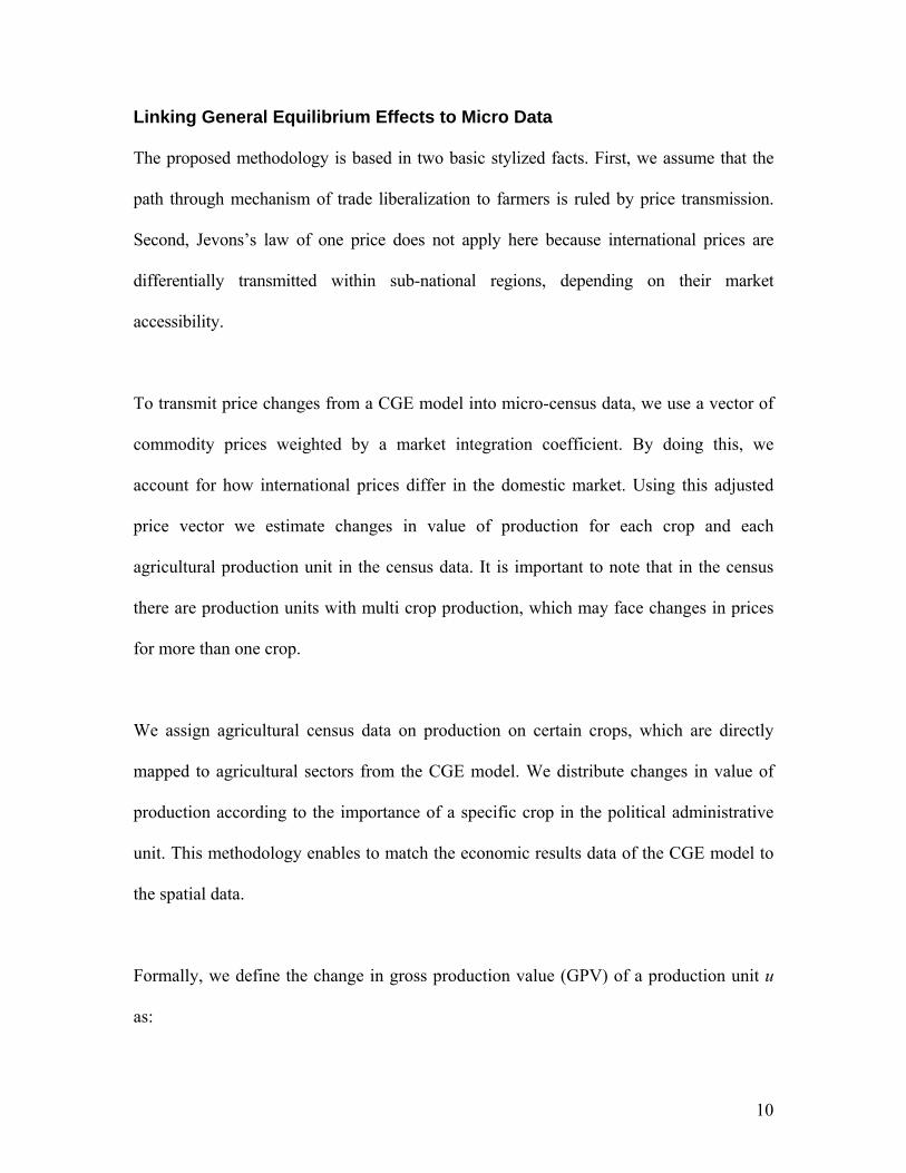
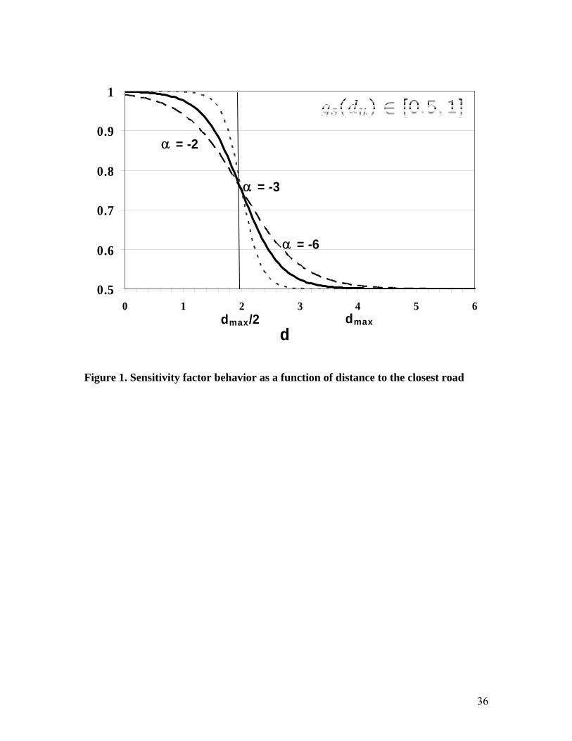
In both cases we assume a logistic curve to model Fu as a function of distance of

production unit u to the closest road that allows farmers marketplace access, du:

(5)

where Fu [a,b], dmax is the maximum distant value that makes the sensitivity factor

negligible, and α is a sensitivity rate that affects the curvature of the function (see figure

1). For practical purposes a value of α = -3 was heuristically chosen for this analysis.

13

Equation (5) allows to model that as distance to road increases, time to point of sale

increases, and if the point of sale is the production unit, price transmission decreases its

influence. As the degree of market integration increases, denoted by farmers selling their

production, the higher the level of price transmission. Thus, the impact of trade

liberalization depends on how changes in border prices are translated into changes in

prices paid to farmers. Price transmission depends on the competitive structure of the

distribution channels, and the extent products are traded. These factors would likely

affect the impacts on different types of farmers (subsistence, traditional and modern

enterprises), as later shown in the results section.

Finally, this methodology to map price changes impacts can be used with both partial

equilibrium and CGE models. However, when aggregation of the agricultural sector is

needed as a whole, it seems that CGE models are a better suited for this purpose.

IV. Economic and Spatial Data

To map the effects of trade liberalization on agriculture, we combine three different data

sources: the results of a CGE model that we link with micro-census data using GIS

software and data. This section describes these three data sources.

A. General Equilibrium Model

The framework used to analyze trade liberalization on the agricultural sector of Ecuador

is a computable general equilibrium model. We use a CGE model with special features

14

for the analysis of agricultural issues, called GTAP-AGR. The Global Trade Analysis

Project (GTAP) model of global trade (Hertel, 1997), is a standard, multi-region, multi-

sector model which includes explicitly treatment of international trade and transport

margins, global savings and investment, and price and income responsiveness across

countries. It assumes perfect competition, constant returns to scale, and an Armington

specification for bilateral trade flows that differentiates trade by origin.

However, critiques argue that the standard GTAP model does not capture some of the

important characteristics of the agricultural economy. To include these special features of

agriculture there is a modified version of the GTAP model and database called GTAP-

AGR (Keeney and Hertel, 2005). The GTAP-AGR model captures certain structural

features of world agricultural markets that are not well reflected in the standard GTAP

model. GTAP-AGR provides a more realistic representation of the farm and food system.

It explicitly identifies farm households as entities that earn income from both farm and

non farm activities, pay taxes, and consume both food and non food products. The model

tries to characterize the degree of factor market segmentation between agriculture and

other sectors of the economy, as well as to improve the representation of input

substitution possibilities in farm production.

In this study we use results from Ludena and Wong (2006) who analyze the impacts of

trade liberalization on Ecuador’s agricultural sector. Specifically, we use price change

information for different agricultural sectors (see Table 1) in the GTAP-AGR database

and link it to micro data, as we explain in the section section.

15

B. Micro Data: Agricultural Census and Prices

The microeconomic data used is the 2000 Agricultural Census data for Ecuador, which is

a representative sample of 150,000 farms. We present the results at the municipal

(canton) level, the third geographical political disaggregation level. This is the highest

political division level of dissagregation at which we can get meaningful averages based

on the sample design and size of the census. The census includes information about land

size, production, use of inputs (land, machinery, labor, seed, etc.), access to credit,

markets and technology, and other variables.

To link these price changes from the CGE model to micro-data from the agricultural

census, we first map sectors in the GTAP-AGR database (Table 2.A) to crops in the

agricultural census. However, the agricultural census does not contain information on

commodity prices. For this reason, we supplemented such information with data from the

National Institute of Statistics and Census (INEC in Spanish). INEC possesses

information on 43 agricultural products, 17 permanent crops and 26 non-perennial crops.

A list of products and their correspondence to general equilibrium sectors is in Tables 2.B

and 2.C. Finally, we estimated the gross value of production (GVP) using census

production data and the price information from INEC.

We supplement this analysis by classifying producers following the same typology used

by Morales et al. (2005). These authors defined three types of Agricultural Production

Units (APU or UPA in Spanish): (i) subsistence farming, (ii) traditional enterprises, and

16

(iii) modern enterprises. This classification is based on producer’s characteristics, as

follows:

i. Subsistence farmers are those who had the following characteristics: a) They

lived in the UPA, b) They did not hire labor, and c) They did not have

machinery (tractors).

ii. Traditional enterprises are defined according to the following attributes: a) They

hired labor, b) they had machinery and c) They did not hire specialized

technical assistance (agronomists, veterinaries, etc).

iii. Finally, modern enterprises are those that additionally to those previous

characteristics, they a) hired specialized technical assistance (agronomists,

veterinaries, etc), b) if it was an individual producer, they had finished basic

and medium education and have some degree of higher education, and c) they

have access to credit.

Tables 3A through 3E offer some insights about these type of producers and their features.

C. GIS Data and Software

The geographically referenced data (third disaggregating level of political division

shapefiles) was provided by the Latin American and Caribbean Demographic Centre

(CELADE) at the Economic Commission for Latin America and the Caribbean

(ECLAC). In our specific case, we map the agricultural census data from Ecuador into

existing polygons that represent each one of the 218 cantons in Ecuador. Geo-referenced

data were stored, managed, analyzed, and displayed by means of the ArcView

commercial software.

17

V. Spatial Representation of the Agricultural Sector in

Ecuador

This section is divided in two main subsections. First, the spatial distribution of

agricultural production in Ecuador based on census data. Second, the spatial distribution

of impacts from trade liberalization on the agricultural sector of Ecuador by region and

type of producer. Both sections are interconnected, as the second builds on the primary

data from the first section in combination with crop price information and data from a

CGE model. We focus our analysis on five crops: rice, soft and hard corn, soybeans and

plant based fibers.

A. Agricultural Production in Ecuador: Crop Maps

This section shows the geographic distribution of crops production by type of producer

based on geographic and climate suitability for crop production of some of the most

important crops in Ecuador. In this paper, the focus is on crops identified by the

government of Ecuador as sensible in a possible free trade agreement with the United

States. These crops include rice, soft corn, hard corn, soybeans (oilseeds) and plant based

fibers (cotton and abaca). Other authors (Larson and Leon, 2006; The World Bank, 2004)

also offer crop mapping for Ecuador, but focused on other crops (rice, potatoes, bananas,

coffee, and cocoa).

Prior to discussing the spatial crop distribution in Ecuador, we first describe the main

agro-ecological zones of Ecuador. This would allow a better understanding of the

18

geographic distribution of crops, as agroecological zones determine the best suitable crop

growing conditions.

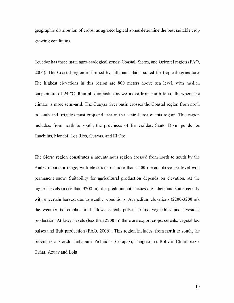
Ecuador has three main agro-ecological zones: Coastal, Sierra, and Oriental region (FAO,

2006). The Coastal region is formed by hills and plains suited for tropical agriculture.

The highest elevations in this region are 800 meters above sea level, with median

temperature of 24 ºC. Rainfall diminishes as we move from north to south, where the

climate is more semi-arid. The Guayas river basin crosses the Coastal region from north

to south and irrigates most cropland area in the central area of this region. This region

includes, from north to south, the provinces of Esmeraldas, Santo Domingo de los

Tsachilas, Manabi, Los Rios, Guayas, and El Oro.

The Sierra region constitutes a mountainous region crossed from north to south by the

Andes mountain range, with elevations of more than 5500 meters above sea level with

permanent snow. Suitability for agricultural production depends on elevation. At the

highest levels (more than 3200 m), the predominant species are tubers and some cereals,

with uncertain harvest due to weather conditions. At medium elevations (2200-3200 m),

the weather is template and allows cereal, pulses, fruits, vegetables and livestock

production. At lower levels (less than 2200 m) there are export crops, cereals, vegetables,

pulses and fruit production (FAO, 2006).. This region includes, from north to south, the

provinces of Carchi, Imbabura, Pichincha, Cotopaxi, Tungurahua, Bolivar, Chimborazo,

Cañar, Azuay and Loja

19

The Oriental region constitutes almost half of Ecuador and is a large drained plain by

rivers that later merge with the Amazon river, with elevations below 600 m. The areas

closest to the Andes have medium temperature of 28 ºC and areas to the east are less

humid and rainy, with higher temperatures. Agricultural production systems of slash and

burn are prominent, with forestry, extensive livestock production and tropical and

subsistence crops as the main agricultural activities. This region includes, from north to

south, the provinces of Sucumbios, Napo, Orellana, Pastaza, Morona Santiago and

Zamora Chinchipe.

To better illustrate the geographic distribution of ecosystems, Figure 2 shows land use by

region. The red areas denote cropland and managed forest, mainly distributed around the

Guayas river basin and in the Sierra region. Green denotes areas under tropical forest,

mainly concentrated in the Oriental region, and north of the Coastal region in the

province of Esmeraldas. Large portions of land under pastures (yellow) are concentrated

in the Sierra region, where livestock and dairy production is located.

In general terms, the crops discussed here, rice, corn, soybeans and cotton are mainly

concentrated in the Coastal region, expect for soft corn production which is located in the

Sierra region. That means that impacts and therefore subsidies, would be focused on

producers around the Guayas river basin, where most of hard corn, rice and soybeans

production is. As we see in the next section, impacts due to the FTA between Ecuador

and the United States follow the geographic distribution of crop location, and are

differentiated by type of producer

20

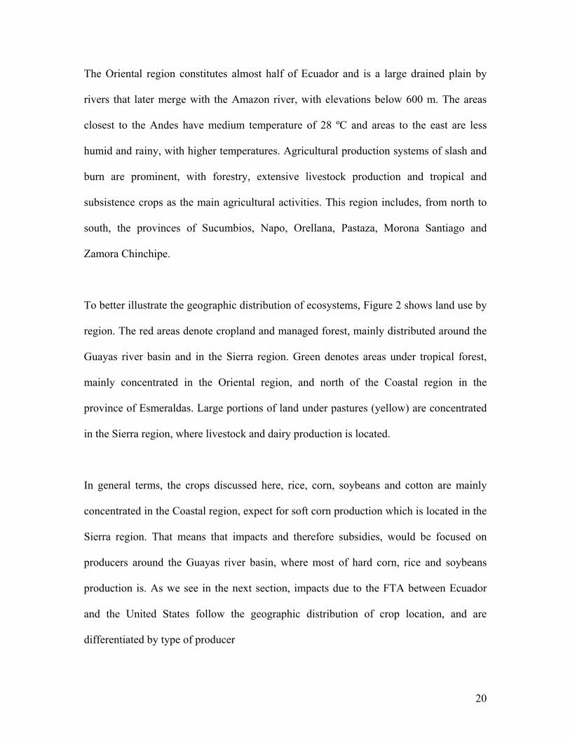
Figures 3 through 12 show the spatial distribution of selected crops in area and number of

UPAs. As discussed before, we focus on five crops: rice, soft corn, hard corn, soybeans

nad plant based fibers (cotton, abaca). We begin our discussion of the geographic

distribution of rice. Rice production in Ecuador occupies the largest area of production

than any other cereal grain crop in Ecuador, and within the Andean countries, Ecuador

has the largest area of rice under production. Rice production has risen in the last 15

years in Ecuador mainly due to the elimination of price controls and a strong export

market in the Andean region (Colombia and Peru).

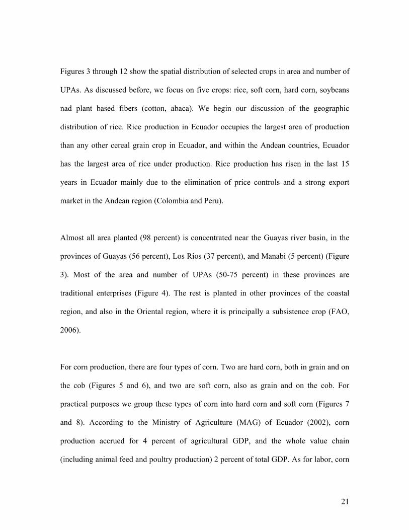
Almost all area planted (98 percent) is concentrated near the Guayas river basin, in the

provinces of Guayas (56 percent), Los Rios (37 percent), and Manabi (5 percent) (Figure

3). Most of the area and number of UPAs (50-75 percent) in these provinces are

traditional enterprises (Figure 4). The rest is planted in other provinces of the coastal

region, and also in the Oriental region, where it is principally a subsistence crop (FAO,

2006).

For corn production, there are four types of corn. Two are hard corn, both in grain and on

the cob (Figures 5 and 6), and two are soft corn, also as grain and on the cob. For

practical purposes we group these types of corn into hard corn and soft corn (Figures 7

and 8). According to the Ministry of Agriculture (MAG) of Ecuador (2002), corn

production accrued for 4 percent of agricultural GDP, and the whole value chain

(including animal feed and poultry production) 2 percent of total GDP. As for labor, corn

21

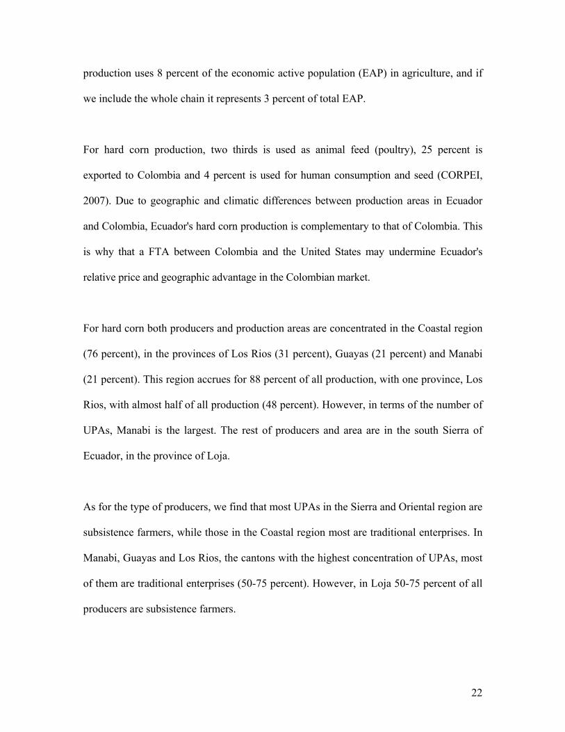
production uses 8 percent of the economic active population (EAP) in agriculture, and if

we include the whole chain it represents 3 percent of total EAP.

For hard corn production, two thirds is used as animal feed (poultry), 25 percent is

exported to Colombia and 4 percent is used for human consumption and seed (CORPEI,

2007). Due to geographic and climatic differences between production areas in Ecuador

and Colombia, Ecuador's hard corn production is complementary to that of Colombia. This

is why that a FTA between Colombia and the United States may undermine Ecuador's

relative price and geographic advantage in the Colombian market.

For hard corn both producers and production areas are concentrated in the Coastal region

(76 percent), in the provinces of Los Rios (31 percent), Guayas (21 percent) and Manabi

(21 percent). This region accrues for 88 percent of all production, with one province, Los

Rios, with almost half of all production (48 percent). However, in terms of the number of

UPAs, Manabi is the largest. The rest of producers and area are in the south Sierra of

Ecuador, in the province of Loja.

As for the type of producers, we find that most UPAs in the Sierra and Oriental region are

subsistence farmers, while those in the Coastal region most are traditional enterprises. In

Manabi, Guayas and Los Rios, the cantons with the highest concentration of UPAs, most

of them are traditional enterprises (50-75 percent). However, in Loja 50-75 percent of all

producers are subsistence farmers.

22

Soft corn production and UPAs are mainly in the Sierra region, with the largest

concentrations in the provinces of Pichincha, Cotopaxi and Chimborazo (Figure 7). For

those UPAs, the majority (50-75 percent) are subsistence farmers. In Azuay and some

cantons of Chimborazo, this percentage increases to 75-100 percent. As for the

distribution of area (Figure 8), Pichincha, Chimborazo, Cotopaxi and Bolivar are the

main production areas. Of those, the majority, especially in Central and South Sierra are

held by subsistence UPAs. This production structure of soft corn, with the majority of

producers both in terms of number of UPAs and area as subsistence farmers would likely

affect the type of policies relative to those for hard corn producers, which are mainly

traditional enterprises.

As for oilseeds (soybeans, sunflower, peanut, raps, and canola), we will focus our

discussion on soybeans, which is the main oilseed crop in Ecuador. Soybean production

is inherently linked to feed production, as soybean cake represents 15-20 percent of feed

composition. According to MAG (2003), in the early 1990's, soybean production

represented 2 percent of agricultural GDP, using 3.7 percent of the economically active

population in agriculture. After those years, there was a decline of soybean production,

mainly due to pests and weather events (El Niño and La Niña).

The areas of oilseed production are concentrated in Manabi and in areas between Loja

and El Oro (Figure 9). Of these UPAs, they are evenly distributed between subsistence

farmers and traditional enterprises (Figure 10). The geographic distribution of production

areas is somewhat different from the distribution of UPAs. Aside from Manabi, El Oro

23

and Loja, there are production areas at the north of Los Rios. Traditional enterprises

make up the majority of area in the provinces of Manabi, El Oro and Loja. In Los Rios,

there is an important share of modern enterprises, in some cantons up to 50-75 percent of

area under production.

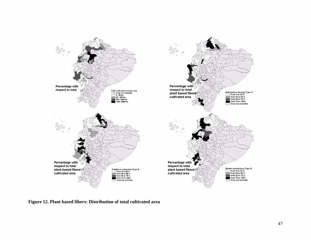
Plant based fibers is composed by cotton, abaca, paja toquilla, and cabuya. Plant based

fibers production is scattered in several provinces of the coastal region, mainly in

Manabi, Guayas, Esmeraldas and Santo Domingo de los Tsachilas. In terms of the

number of UPAs, they are scattered throughout the Coastal region, with no identifiable

pattern in the geographic distribution of producers (Figure 11). For cotton, which is the

main product within this group, production is concentrated in two provinces, Manabi (52

percent) and Guayas (47 percent). However, of the total number of UPAs, almost two

thirds are in Guayas and one third in Manabi.

B. Spatial Distribution of Trade Liberalization Impacts on Agriculture

After discussing the geographic distribution of agricultural production areas in Ecuador

for sensitivity products (rice, corn, soybeans, plant based fibers), this section shows the

spatial distribution of impacts of trade liberalization on farmers of these products. This by

no means is a complete picture of the total effects in the value of production, since we do

not account for the change in production (quantities) that may happen.

Before discussing the results, we present a map of market access to helps us better

understand some of the results of impacts, which are determined by farmers’ market

24

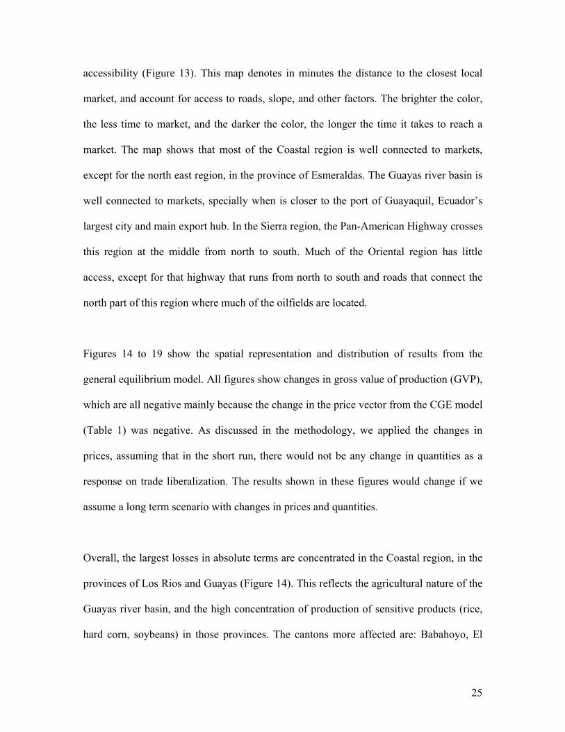
accessibility (Figure 13). This map denotes in minutes the distance to the closest local

market, and account for access to roads, slope, and other factors. The brighter the color,

the less time to market, and the darker the color, the longer the time it takes to reach a

market. The map shows that most of the Coastal region is well connected to markets,

except for the north east region, in the province of Esmeraldas. The Guayas river basin is

well connected to markets, specially when is closer to the port of Guayaquil, Ecuador’s

largest city and main export hub. In the Sierra region, the Pan-American Highway crosses

this region at the middle from north to south. Much of the Oriental region has little

access, except for that highway that runs from north to south and roads that connect the

north part of this region where much of the oilfields are located.

Figures 14 to 19 show the spatial representation and distribution of results from the

general equilibrium model. All figures show changes in gross value of production (GVP),

which are all negative mainly because the change in the price vector from the CGE model

(Table 1) was negative. As discussed in the methodology, we applied the changes in

prices, assuming that in the short run, there would not be any change in quantities as a

response on trade liberalization. The results shown in these figures would change if we

assume a long term scenario with changes in prices and quantities.

Overall, the largest losses in absolute terms are concentrated in the Coastal region, in the

provinces of Los Rios and Guayas (Figure 14). This reflects the agricultural nature of the

Guayas river basin, and the high concentration of production of sensitive products (rice,

hard corn, soybeans) in those provinces. The cantons more affected are: Babahoyo, El

25

Guabo, Naranjal, Valencia, Ventanas, Machala, Baba, La Troncal, Puebloviejo, Pasaje

and Buena Fe.

The most interesting result is that of those mostly affected in those areas and cantons, the

majority of producers are modern enterprises. This reflects the nature of the production

systems in those areas, and the market linkage that these modern enterprises have relative

to subsistence farmers and traditional enterprises. Given that modern enterprises are more

linked to exports markets (especially rice producers), any shock in international prices

will be transmitted almost entirely to these producers. That is not the case for subsistence

farmers, that although may have access to roads, selling to intermediaries reduces the

price transmission shocks from international markets. Traditional enterprises make up

most of those affected in the provinces of Manabi, Esmeraldas, Loja, central Sierra

provinces and the northern provinces of the Oriental region. Subsistence farmers make up

most of those losing in the southern Sierra (especially Azuay) and in the Oriental region.

As we look the change in GVP by crop, we observe that rice loses are mainly

concentrated in Los Rios and Guayas (Figure 15). The cantons more affected are

Babahoyo, Daule, Sanborondon, Santa Lucia, Urbina Jado, Yaguachi and Naranjal. Most

of the producers in those cantons with high losses are mainly modern enterprises and

traditional enterprises, which as discussed before, are more connected with export

markets. These results reflect the concern of the Ecuadorian government of losing the

exports markets of Colombia and Peru to imports from the United States. The most

affected producers may well be those modern enterprises.

26

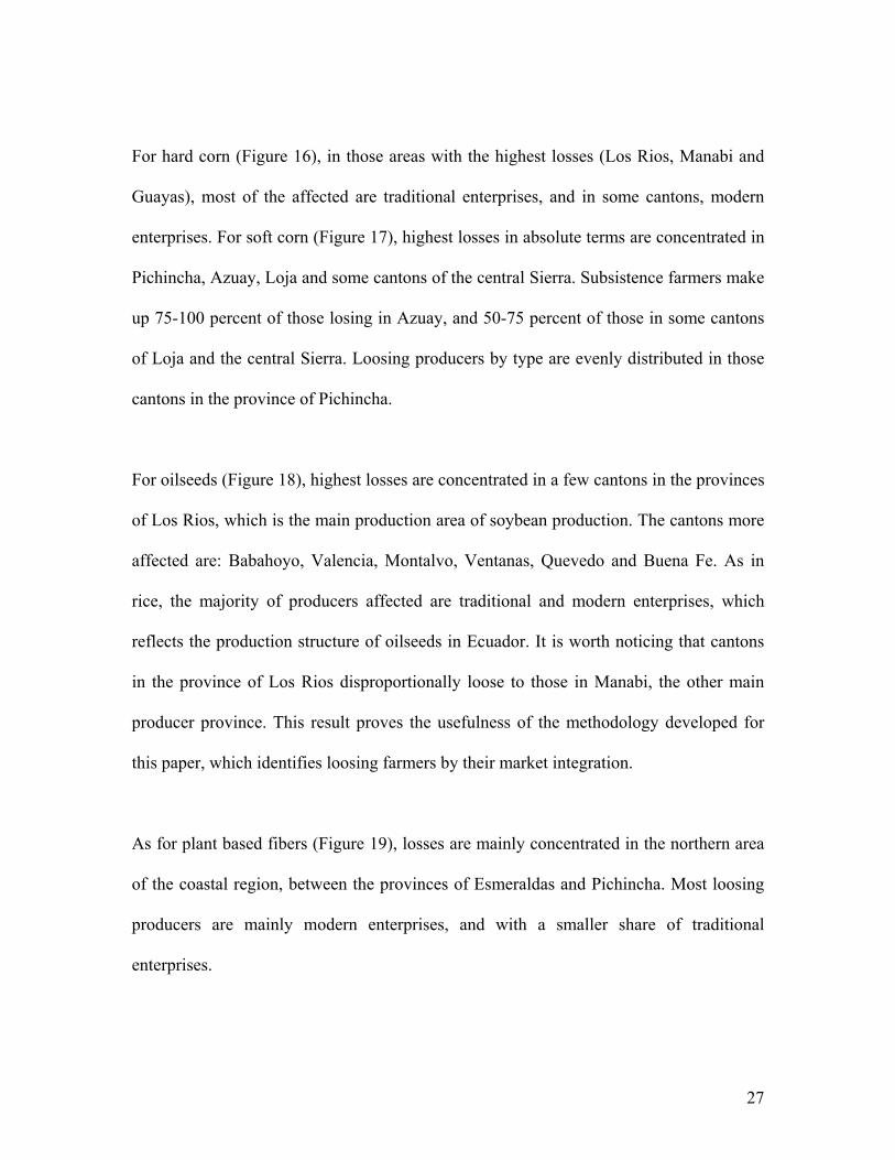
For hard corn (Figure 16), in those areas with the highest losses (Los Rios, Manabi and

Guayas), most of the affected are traditional enterprises, and in some cantons, modern

enterprises. For soft corn (Figure 17), highest losses in absolute terms are concentrated in

Pichincha, Azuay, Loja and some cantons of the central Sierra. Subsistence farmers make

up 75-100 percent of those losing in Azuay, and 50-75 percent of those in some cantons

of Loja and the central Sierra. Loosing producers by type are evenly distributed in those

cantons in the province of Pichincha.

For oilseeds (Figure 18), highest losses are concentrated in a few cantons in the provinces

of Los Rios, which is the main production area of soybean production. The cantons more

affected are: Babahoyo, Valencia, Montalvo, Ventanas, Quevedo and Buena Fe. As in

rice, the majority of producers affected are traditional and modern enterprises, which

reflects the production structure of oilseeds in Ecuador. It is worth noticing that cantons

in the province of Los Rios disproportionally loose to those in Manabi, the other main

producer province. This result proves the usefulness of the methodology developed for

this paper, which identifies loosing farmers by their market integration.

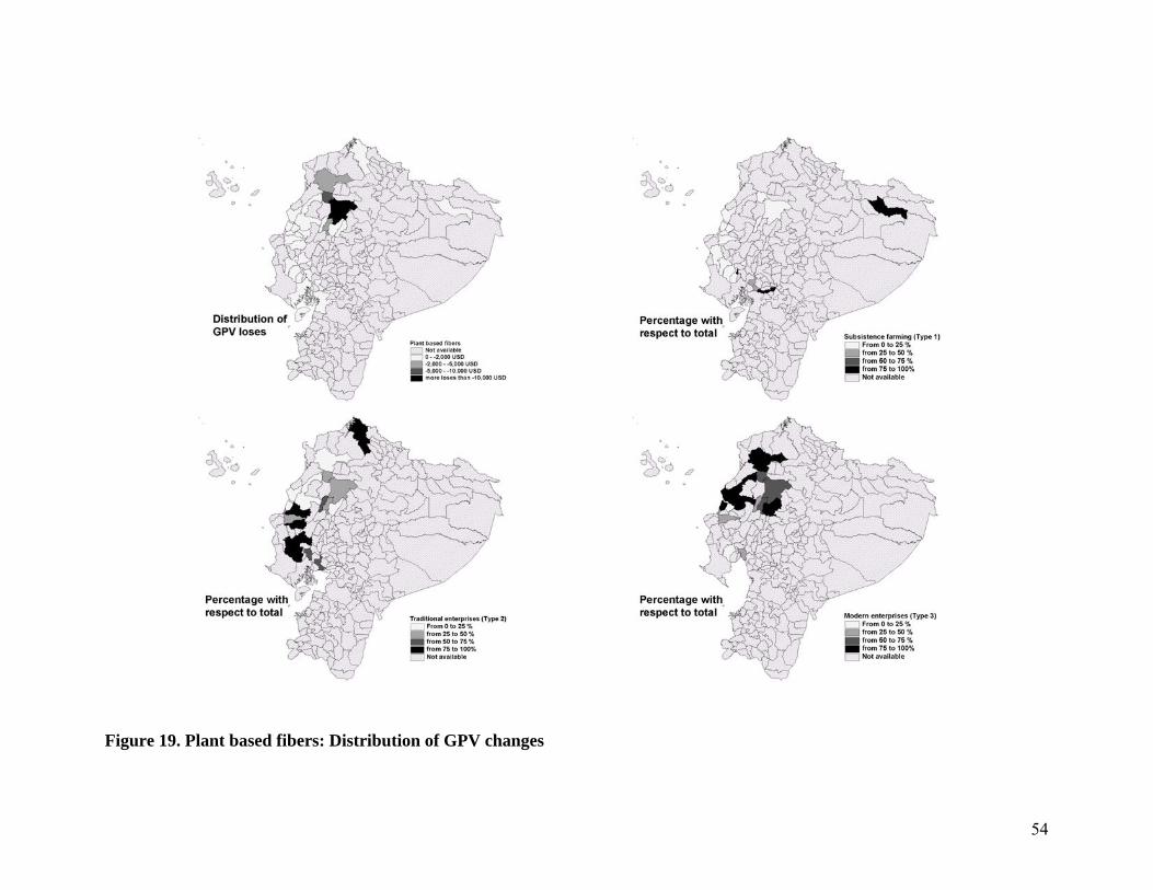
As for plant based fibers (Figure 19), losses are mainly concentrated in the northern area

of the coastal region, between the provinces of Esmeraldas and Pichincha. Most loosing

producers are mainly modern enterprises, and with a smaller share of traditional

enterprises.

27

Finally, government’s compensation policies should follow the same spatial pattern

outlined by the results presented in this section. As the results show, for the majority of

crops analyzed, some of the most affected producers are those classified as modern

enterprises. This has important implications for policy makers, since in most cases,

policies and subsidies are focused on those smaller producers that cannot stand for

themselves. Modern enterprises may be able to better change and adapt to the new

situations produced by trade liberalization, which may not be true for subsistence

farmers. However, and as shown in our results, the focus of policies may as well be

modern enterprises, at least during transitional periods.

VI. Conclusions

In this study we have shown the results of an applied general equilibrium model through

the spatial lens. To do this we have developed a methodology that enables us to merge the

CGE results with microeconomic information. We have applied this methodology to the

effects of a free trade agreement between Ecuador and the United States on Ecuador’s

agriculture. We show that most producers and area of the crops that would be the focus of

compensation policies (rice, corn and soybeans) are mainly around the basin of the

Guayas river basin in the provinces of Guayas, Los Rios and Manabi.

The spatial distribution of impacts in Ecuador of the trade agreements studied in this

paper could be used to analyze and implement possible compensation policies to mitigate

its potential negative impacts. Explicitly, these targeted policies should be mostly focused

in the Guayas river basin, where most producers of cereals and oilseeds are. Rice, hard

28

corn and soybeans production areas and producers are concentrated in Guayas, Los Rios

and Manabi. Soft corn producers are mainly concentrated in the Sierra region, especially

in the central and south areas. Moreover, the government should make a clear distinction

between subsistence farmers, traditional and modern enterprises, focusing in subsistence

and traditional enterprises because modern enterprises have more capability of adapting

to changes from trade liberalization. For subsistence farmers any compensation policy

should be complemented with a widespread social policy that enable them improve their

access to basic sanitation infrastructure, health services, basic education and capacity

building in agricultural issues.

The methodology developed in this study would enable policy makers to focus their

policies by means of geo-referenced impact outcomes. The use of this tool with other

geographically referenced data (such as income or weather data) would be of great use

for policies ranging from poverty reduction to environmental mitigation of global

warming in order to spur advances towards the achievement of the Millennium

Development Goals and the required sustainable development of the country. For that

reason, future improvements of this tool plans to combine other geographically

referenced data, such as household surveys with socio-economic information that would

enable policy makers to better target specific policies to where they are most needed.

Several areas of future research may improve the methodology developed in this paper.

The distribution of impacts should be based more on empirical and econometric work.

Market integration and spatial price transmission tests should be a first step in that

29

direction. This is important to estimate the parameters used in the logistic function which

has been chosen heuristically. In addition, we need to be able to distinguish between the

different channels of commercialization, and determine whether there are sensible

differences between the type of market channel and prices. Also, it is important to

improve price information and regional price distribution, by means of countrywide

prices surveys that cover all the cantons and products. Finally, the methodology could

also improve by including a mechanism that accounts for changes in production

quantities at the UPA level. Such mechanism could include a microsimulation procedure

such as Monte Carlo simulation methods.

Through the use of the Agricultural Census and the GIS geo-referenced process,

agricultural sectoral impacts has disaggregated and registered into individual locations, in

our case, cantons. The visualization of this disaggregated information by means of GIS

techniques would enable decision makers to display the results of the policies to be

applied and consequently improve the quality of their choices. This is especially

important in the agro-business sector where the productive units reside along the whole

country territory. Visualization helps not only in obtaining a systemic view of a subject

matter but also to improve the quality of communication among stakeholders. Also, the

integration between GIS and CGE analysis makes it possible to capture additional

information which is not included in the macro analysis.

We expect that the hybrid combination of macro analysis techniques, such as CGE

modeling with micro or geographically disaggregated data will be the next useful step

30

toward the better understanding of transmission mechanisms of economic policies so as

to assist the informed policy interventions in issues such as poverty reduction,

deforestation, efficient and environmentally friendly use of land and adaptation and

mitigation strategies of climate change.

31

References

Asadoorian, M.O. 2005. “Simulating the Spatial Distribution of Population and

Emissions to 2100.” MIT Joint Program on the Science and Policy of Global

Change. Report No. 123.

CORPEI. 2007. “Maíz.” http://www.corpei.org/FrameCenter.asp?Ln=SP&

Opcion=3_3_6. Exports and Investment Promotion Corporation of Ecuador

(CORPEI).

Durán, J., A. Schuschny and C. de Miguel. 2006. “Andean Countries and the USA: How

much can be expected from FTAs.” ECLAC, United Nations.

Dixon, P., M.T. Rimmer, and M. Tsigas. 2004. “Macro, industry, and state effects in the

U.S. of removing major tariffs and quotas.” Studies and the Impact Project.

General Working Paper No. G-146.

Escobal, L. 2001. “The benefits of roads in rural Peru: a transaction costs approach.”

Grupo de Análisis para el Desarrollo (GRADE), Lima.

FAO. 2006. “Calendario de cultivos: América Latina y el Caribe.” Estudio FAO

Producción y Protección Vegetal No. 186. Organización de las Naciones Unidas

para la Agricultura y la Alimentación, Roma.

Ferreira Filho, J.B., y M. Horridge. 2005. “The Doha Round, Poverty, and Regional

Inequality in Brazil.” In Poverty and the WTO: Impacts of the Doha Development

Agenda. Washington: T.W. Hertel and L.A. Winters, eds, pp. 183-218.

Haddad, E. and F. Perobelli. 2005. “Trade Liberalization and Regional Inequality: Do

Transportation Costs Impose a Spatial Poverty Trap?” Eighth Annual Conference

on Global Economic Analysis. Lübeck, Germany. June, 2005.

32

Hertel, T.W. 1997. Global Trade Analysis: Modeling and Applications, Cambridge

University Press.

INEC. 2006. “Encuesta de superficie y producción agropecuaria continua.” Sistema

Estadístico Agropecuario Nacional, Instituto Nacional de Estadísticas y Censos

(INEC). Quito, septiembre 2006.

Keeney, R. and T.W. Hertel. 2005. “GTAP-AGR: A framework for assessing the

implications of multilateral changes in agricultural policies.” GTAP Technical

Paper No. 24. Center of Global Trade Analysis, Purdue University.

Kjöllerström, M. 2004. “Liberalización comercial agrícola con costos de transporte y

transacción elevados: evidencia para América Latina.” Unidad de Desarrollo

Agrícola, División de Desarrollo Productivo y Empresarial, CEPAL.

Larson, D.F. and M. Leon. 2006. “How endowments, accumulations, and choice

determine the geography of agricultural productivity in Ecuador.” The World

Bank Economic Review, 20(3):449-471

Lee, H., T.W. Hertel, B. Sohngen and N. Ramankutty. 2005. “Towards an integrated land

use database for assessing the potential for greenhouse gas mitigation.” GTAP

Technical Paper No. 25. Center of Global Trade Analysis, Purdue University.

Leon, M. and N. Shady. 2003. “Metodología para la estimación monetaria de la

producción agrícola.” Mimeo.

Ludena, C.E. and S. Wong. 2006. “Domestic support policies for agriculture in Ecuador

and the U.S.-Andean countries free trade agreement: an applied general

equilibrium assessment.” Contributed paper prepared for presentation at the Ninth

33

Annual Conference on Global Economic Analysis, Addis Ababa, Ethiopia, June

2006.

Ministry of Agriculture of Ecuador (MAG). 2002. “Ecuador: panorama de la cadena de

maíz, hacia donde vamos?”

http://www.sica.gov.ec/cadenas/maiz/docs/panorama_cadena2002.html. (accessed

March 2007)

Ministry of Agriculture of Ecuador (MAG). 2003. “Panorama de la cadena de soya.”

http://www.sica.gov.ec/cadenas/soya/docs/panorama_soya2003.htm (accessed

March 2007)

McMillan, M., D. Rodrik, and K.H. Welch. 2002. “When economic reform goes wrong:

cashews in Mozambique.” NBER Working Paper 9117, NBER, Cambridge, MA.

Morales, C., S. Parada, M. Torres, M. Rodrigues, and J.E. Faundez. 2005. “Los impactos

diferenciados del Tratado de Libre Comercio Ecuador – Estados Unidos de Norte

América sobre la agricultura del Ecuador.” Unidad de Desarrollo Agrícola,

División de Desarrollo Productivo y Empresarial, CEPAL.

Nicita, A. 2004. “Who benefited from trade liberalization in Mexico? Measuring the

effects on household welfare.” World Bank Working Papers 3265.

Nicita, A. 2005. “Multilateral trade liberalization and Mexican households: the effect of

the Doha Development Agenda.” In Poverty and the WTO: Impacts of the Doha

Development Agenda. Washington: T.W. Hertel and L.A. Winters, eds, 107-128.

Salceso, S. 2007. Personal communication.

Schuschny, A. and G. Gallopin. 2004. “La distribución espacial de la pobreza en relación

a los sistemas ambientales en América Latina.” Serie Medio Ambiente y

34

Desarrollo No. 87, CEPAL, Naciones Unidas,

http://www.cepal.org/id.asp?id=15490.

Sheldon, I. 2006. “Market structure, industrial concentration, and price transmission.”

Paper prepared for presentation at workshop on “Market Integration and Vertical

and Spatial Price Transmission in Agricultural Markets”, University of Kentucky,

Lexington, KY, 21st April, 2006.

The World Bank. 2004. “Rural poverty, agricultural productivity, and the distribution of

land.” In Ecuador Poverty Assessment. Poverty Reduction and Economic

Management Sector Unit, Latin America and the Caribbean Region

Vakis, R. E. Sadoulet, and A. de Janvry. 2003. “Measuring transactions costs from

observed behavior: market choices in Peru.” The World Bank and Department of

Agricultural and Resource Economics, University of California at Berkeley.

35

0.5

0.6

0.7

0.8

0.9

1

0 1 2 3 4 5dmaxdmax/2

d

= -3

= -6

= -2

6

Figure 1. Sensitivity factor behavior as a function of distance to the closest road

36

37

Figure 2. Vegetation cover and cropland areas in Ecuador

Source: Global Land Cover (http://www-gvm.jrc.it/glc2000/defaultGLC2000.htm)

.

Figure 3. Paddy rice: Distribution of UPAs

38

Figure 4. Paddy rice: Distribution of total cultivated area

39

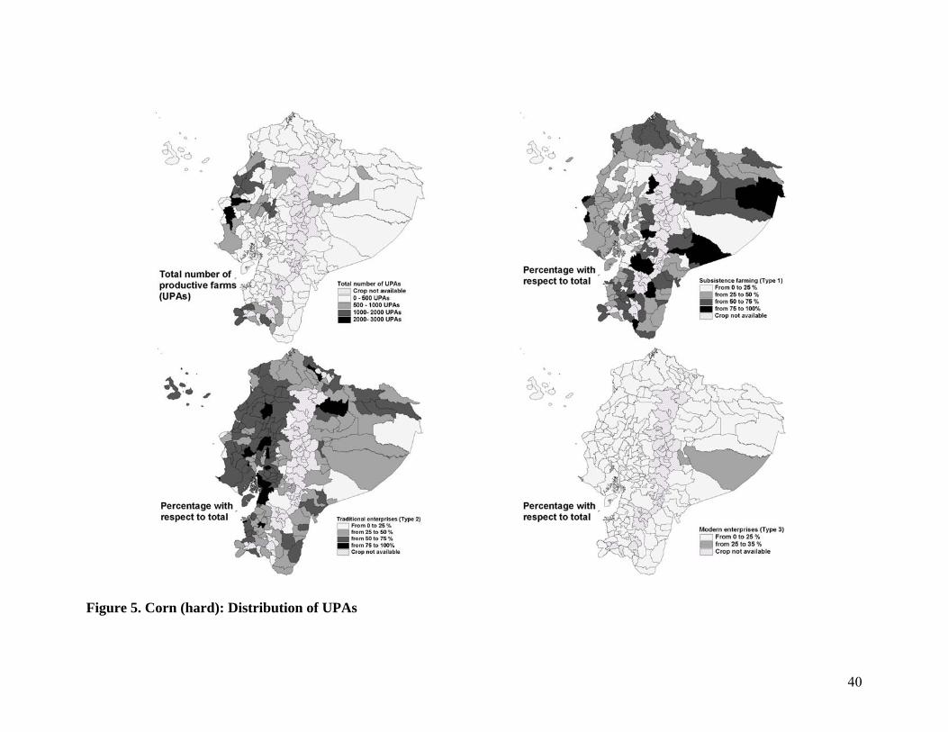
Figure 5. Corn (hard): Distribution of UPAs

40

Figure 6. Corn (hard): Distribution of total cultivated area

41

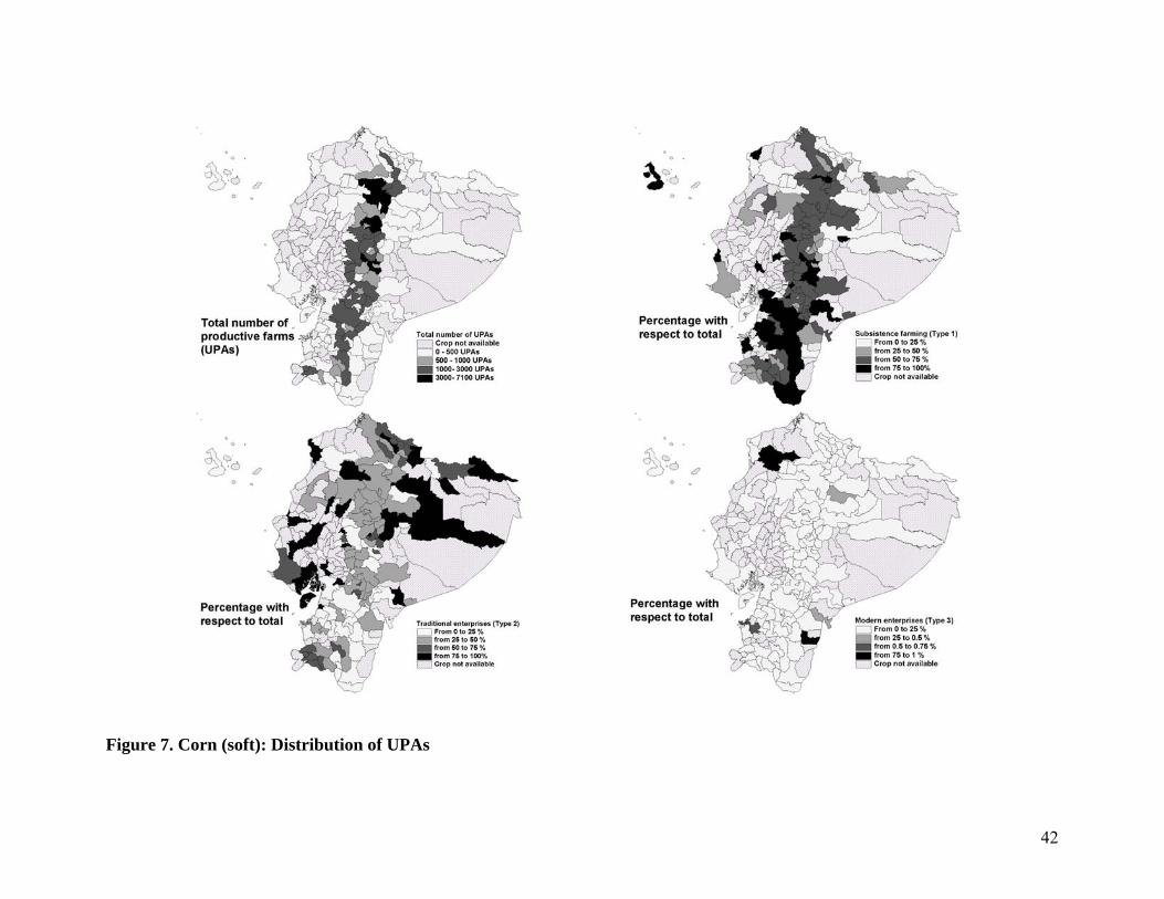
Figure 7. Corn (soft): Distribution of UPAs

42

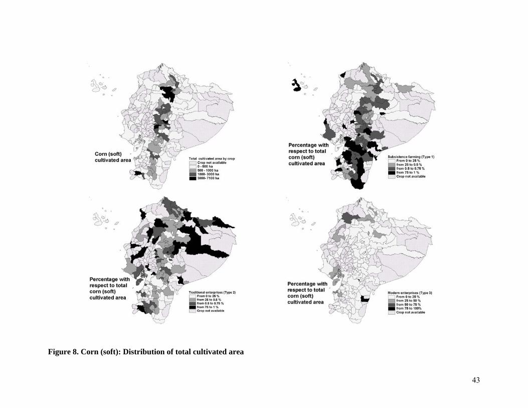
Figure 8. Corn (soft): Distribution of total cultivated area

43

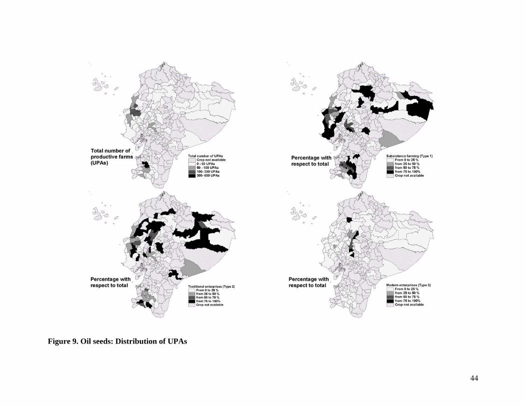
Figure 9. Oil seeds: Distribution of UPAs

44

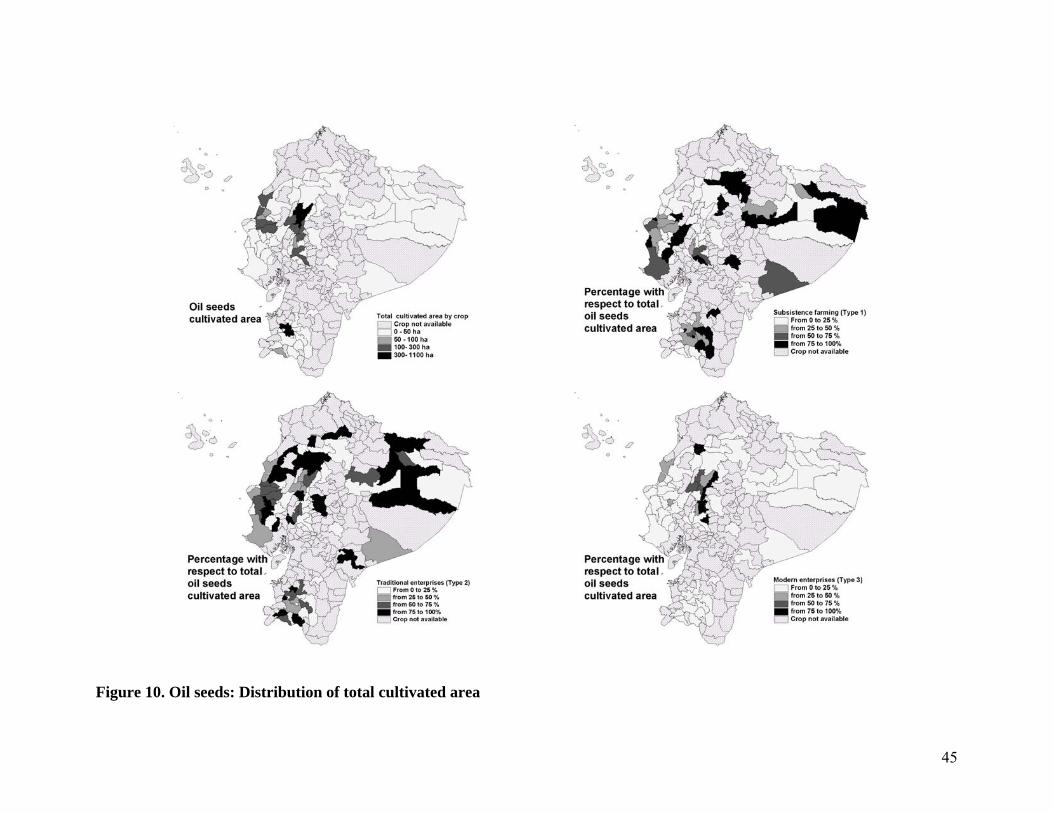
Figure 10. Oil seeds: Distribution of total cultivated area

45

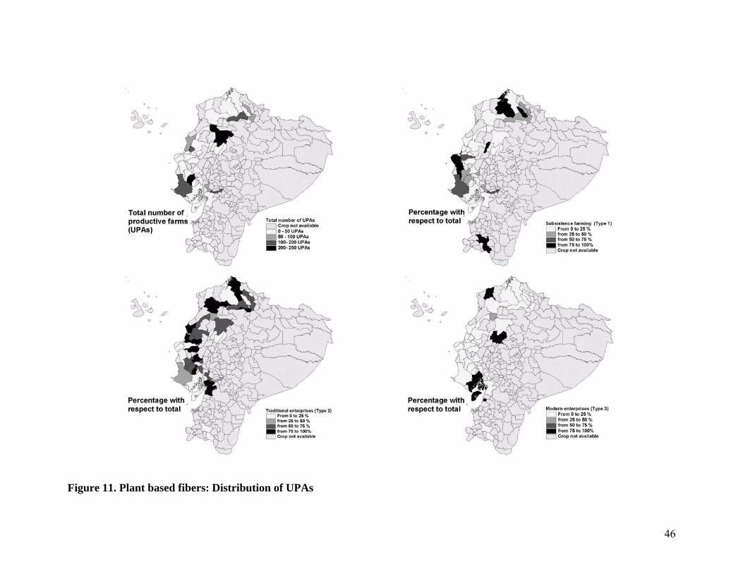
Figure 11. Plant based fibers: Distribution of UPAs

46

47

Figure 12. Plant based fibers: Distribution of total cultivated area

Figure 13. Accessibility to local markets in Ecuador Source: CIAT (2004), available from http://www.ecuamapalimentaria.info.

48

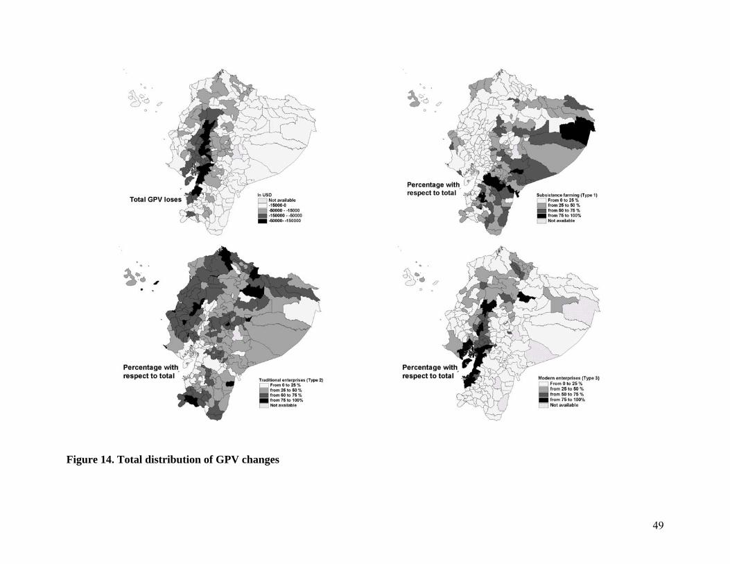
Figure 14. Total distribution of GPV changes

49

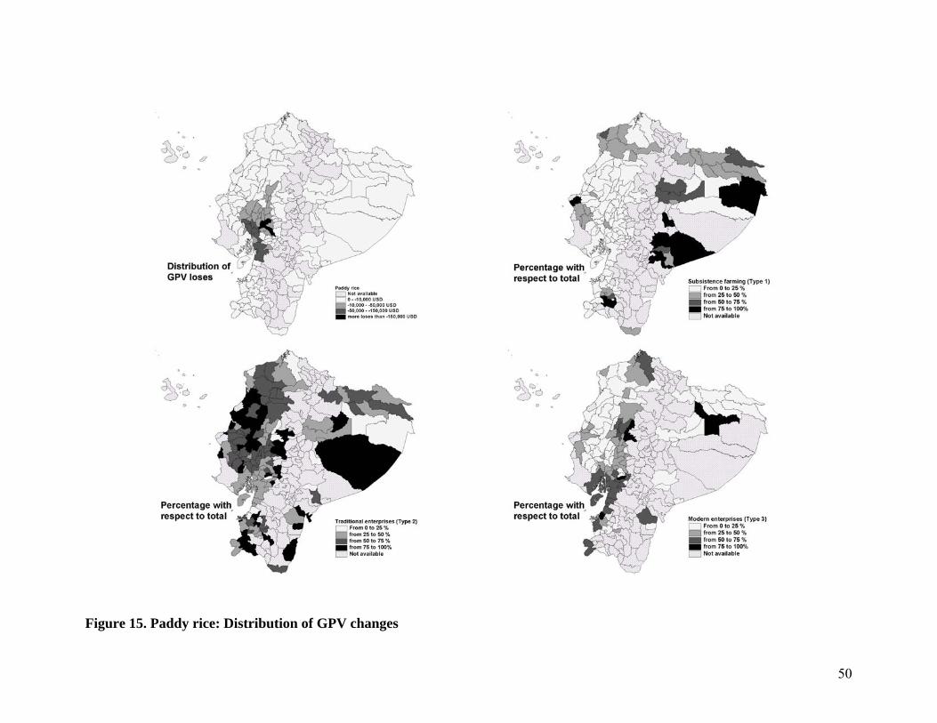
Figure 15. Paddy rice: Distribution of GPV changes

50

Figure 16. Corn (hard): Distribution of GPV changes

51

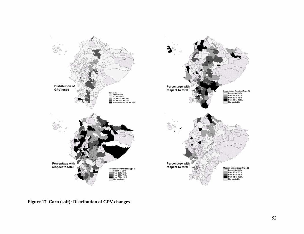
Figure 17. Corn (soft): Distribution of GPV changes

52

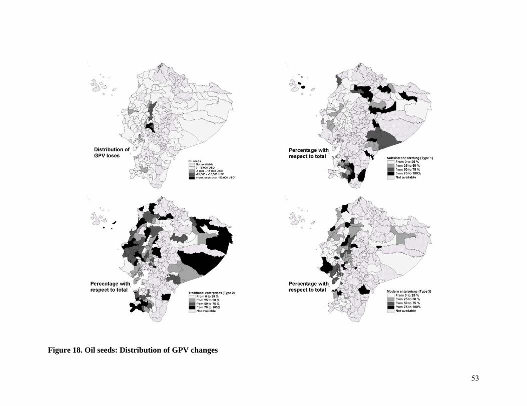
Figure 18. Oil seeds: Distribution of GPV changes

53

54

Figure 19. Plant based fibers: Distribution of GPV changes

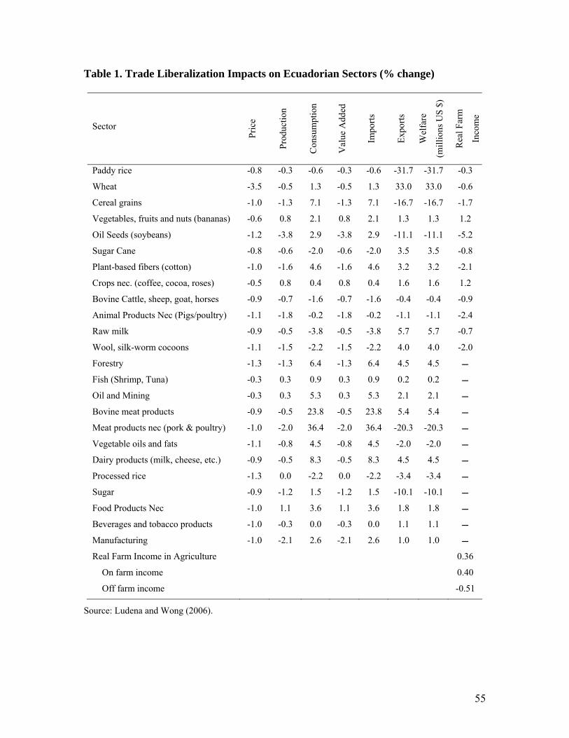
Table 1. Trade Liberalization Impacts on Ecuadorian Sectors (% change)

Sector

Pri

ce

Pro

duct

ion

Con

sum

ptio

n

Val

ue A

dded

Impo

rts

Exp

orts

Wel

fare

(mil

lion

s U

S $

)

Rea

l Far

m

Inco

me

Paddy rice -0.8 -0.3 -0.6 -0.3 -0.6 -31.7 -31.7 -0.3

Wheat -3.5 -0.5 1.3 -0.5 1.3 33.0 33.0 -0.6

Cereal grains -1.0 -1.3 7.1 -1.3 7.1 -16.7 -16.7 -1.7

Vegetables, fruits and nuts (bananas) -0.6 0.8 2.1 0.8 2.1 1.3 1.3 1.2

Oil Seeds (soybeans) -1.2 -3.8 2.9 -3.8 2.9 -11.1 -11.1 -5.2

Sugar Cane -0.8 -0.6 -2.0 -0.6 -2.0 3.5 3.5 -0.8

Plant-based fibers (cotton) -1.0 -1.6 4.6 -1.6 4.6 3.2 3.2 -2.1

Crops nec. (coffee, cocoa, roses) -0.5 0.8 0.4 0.8 0.4 1.6 1.6 1.2

Bovine Cattle, sheep, goat, horses -0.9 -0.7 -1.6 -0.7 -1.6 -0.4 -0.4 -0.9

Animal Products Nec (Pigs/poultry) -1.1 -1.8 -0.2 -1.8 -0.2 -1.1 -1.1 -2.4

Raw milk -0.9 -0.5 -3.8 -0.5 -3.8 5.7 5.7 -0.7

Wool, silk-worm cocoons -1.1 -1.5 -2.2 -1.5 -2.2 4.0 4.0 -2.0

Forestry -1.3 -1.3 6.4 -1.3 6.4 4.5 4.5

Fish (Shrimp, Tuna) -0.3 0.3 0.9 0.3 0.9 0.2 0.2

Oil and Mining -0.3 0.3 5.3 0.3 5.3 2.1 2.1

Bovine meat products -0.9 -0.5 23.8 -0.5 23.8 5.4 5.4

Meat products nec (pork & poultry) -1.0 -2.0 36.4 -2.0 36.4 -20.3 -20.3

Vegetable oils and fats -1.1 -0.8 4.5 -0.8 4.5 -2.0 -2.0

Dairy products (milk, cheese, etc.) -0.9 -0.5 8.3 -0.5 8.3 4.5 4.5

Processed rice -1.3 0.0 -2.2 0.0 -2.2 -3.4 -3.4

Sugar -0.9 -1.2 1.5 -1.2 1.5 -10.1 -10.1

Food Products Nec -1.0 1.1 3.6 1.1 3.6 1.8 1.8

Beverages and tobacco products -1.0 -0.3 0.0 -0.3 0.0 1.1 1.1

Manufacturing -1.0 -2.1 2.6 -2.1 2.6 1.0 1.0

Real Farm Income in Agriculture 0.36

On farm income 0.40

Off farm income -0.51

Source: Ludena and Wong (2006).

55

Table 2.A. Commodity Aggregation and correspondence of Ecuador’s Agricultural Sectors to GTAP Sectors No. GTAP Sector Description Ecuador Sectors Analyzed

1 pdr Paddy Rice Paddy rice

2 wht Wheat Wheat

Corn – hard

Corn – soft

3 gro Cereal Grains Nec. (corn, rye)

Other cereals

Fruits 4 v_f Vegetables, fruits and nuts (bananas)

Vegetables

5 osd Oil Seeds (soybeans) Oil seeds

6 c_b Sugar Cane Sugar crops

7 pfb Plant-based fibers (cotton) Plant based fibers

Roses

Coffee

Cacao

8 ocr Crops nec. (coffee, cacao, roses)

Other crops

9 ctl Bovine Cattle, sheeps, goats horses

10 oap Animal Products Nec (Pigs, poultry)

11 rmk Raw Milk

12 wol Wool, silk-worm cocoons

13 for Forestry

14 fsh Fishing (Shrimp, Tuna)

15 Oil and Mining Oil and Mining

16 cmt Bovine meat products

17 omt Meat products nec (pork, poultry meat)

18 vol Vegetable oils and fats

19 mil Dairy products (milk, cheese, etc.)

20 pcr Processed rice

21 sgr Sugar

22 ofd Food Products Nec

23 b_t Beverages and tobacco products

24 Manufacturing Manufacturing

25 Services Services

56

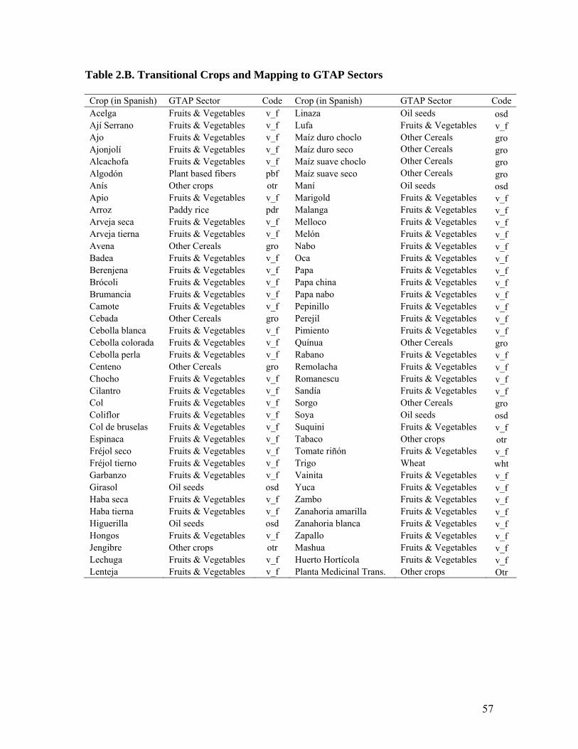
Table 2.B. Transitional Crops and Mapping to GTAP Sectors Crop (in Spanish) GTAP Sector Code Crop (in Spanish) GTAP Sector Code Acelga Fruits & Vegetables v_f Linaza Oil seeds osd Ají Serrano Fruits & Vegetables v_f Lufa Fruits & Vegetables v_f Ajo Fruits & Vegetables v_f Maíz duro choclo Other Cereals gro Ajonjolí Fruits & Vegetables v_f Maíz duro seco Other Cereals gro Alcachofa Fruits & Vegetables v_f Maíz suave choclo Other Cereals gro Algodón Plant based fibers pbf Maíz suave seco Other Cereals gro Anís Other crops otr Maní Oil seeds osd Apio Fruits & Vegetables v_f Marigold Fruits & Vegetables v_f Arroz Paddy rice pdr Malanga Fruits & Vegetables v_f Arveja seca Fruits & Vegetables v_f Melloco Fruits & Vegetables v_f Arveja tierna Fruits & Vegetables v_f Melón Fruits & Vegetables v_f Avena Other Cereals gro Nabo Fruits & Vegetables v_f Badea Fruits & Vegetables v_f Oca Fruits & Vegetables v_f Berenjena Fruits & Vegetables v_f Papa Fruits & Vegetables v_f Brócoli Fruits & Vegetables v_f Papa china Fruits & Vegetables v_f Brumancia Fruits & Vegetables v_f Papa nabo Fruits & Vegetables v_f Camote Fruits & Vegetables v_f Pepinillo Fruits & Vegetables v_f Cebada Other Cereals gro Perejil Fruits & Vegetables v_f Cebolla blanca Fruits & Vegetables v_f Pimiento Fruits & Vegetables v_f Cebolla colorada Fruits & Vegetables v_f Quínua Other Cereals gro Cebolla perla Fruits & Vegetables v_f Rabano Fruits & Vegetables v_f Centeno Other Cereals gro Remolacha Fruits & Vegetables v_f Chocho Fruits & Vegetables v_f Romanescu Fruits & Vegetables v_f Cilantro Fruits & Vegetables v_f Sandía Fruits & Vegetables v_f Col Fruits & Vegetables v_f Sorgo Other Cereals gro Coliflor Fruits & Vegetables v_f Soya Oil seeds osd Col de bruselas Fruits & Vegetables v_f Suquini Fruits & Vegetables v_f Espinaca Fruits & Vegetables v_f Tabaco Other crops otr Fréjol seco Fruits & Vegetables v_f Tomate riñón Fruits & Vegetables v_f Fréjol tierno Fruits & Vegetables v_f Trigo Wheat wht Garbanzo Fruits & Vegetables v_f Vainita Fruits & Vegetables v_f Girasol Oil seeds osd Yuca Fruits & Vegetables v_f Haba seca Fruits & Vegetables v_f Zambo Fruits & Vegetables v_f Haba tierna Fruits & Vegetables v_f Zanahoria amarilla Fruits & Vegetables v_f Higuerilla Oil seeds osd Zanahoria blanca Fruits & Vegetables v_f Hongos Fruits & Vegetables v_f Zapallo Fruits & Vegetables v_f Jengibre Other crops otr Mashua Fruits & Vegetables v_f Lechuga Fruits & Vegetables v_f Huerto Hortícola Fruits & Vegetables v_f Lenteja Fruits & Vegetables v_f Planta Medicinal Trans. Other crops Otr

57

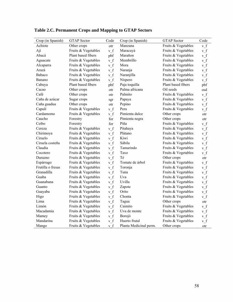
Table 2.C. Permanent Crops and Mapping to GTAP Sectors Crop (in Spanish) GTAP Sector Code Crop (in Spanish) GTAP Sector Code Achiote Other crops otr Manzana Fruits & Vegetables v_f Ají Fruits & Vegetables v_f Maracuyá Fruits & Vegetables v_f Abacá Plant based fibers pbf Marañon Fruits & Vegetables v_f Aguacate Fruits & Vegetables v_f Membrillo Fruits & Vegetables v_f Alcaparra Fruits & Vegetables v_f Mora Fruits & Vegetables v_f Arazá Fruits & Vegetables v_f Naranja Fruits & Vegetables v_f Babaco Fruits & Vegetables v_f Naranjilla Fruits & Vegetables v_f Banano Fruits & Vegetables v_f Níspero Fruits & Vegetables v_f Cabuya Plant based fibers pbf Paja toquilla Plant based fibers pbf Cacao Other crops otr Palma africana Oil seeds osd Café Other crops otr Palmito Fruits & Vegetables v_f Caña de azúcar Sugar crops sgr Papaya Fruits & Vegetables v_f Caña guadua Other crops otr Pepino Fruits & Vegetables v_f Capulí Fruits & Vegetables v_f Pera Fruits & Vegetables v_f Cardamomo Fruits & Vegetables v_f Pimienta dulce Other crops otr Caucho Forestry for Pimienta negra Other crops otr Ceibo Forestry for Piña Fruits & Vegetables v_f Cereza Fruits & Vegetables v_f Pitahaya Fruits & Vegetables v_f Chirimoya Fruits & Vegetables v_f Plátano Fruits & Vegetables v_f Ciruelo Fruits & Vegetables v_f Kiwi Fruits & Vegetables v_f Ciruela costeña Fruits & Vegetables v_f Sábila Fruits & Vegetables v_f Claudia Fruits & Vegetables v_f Tamarindo Fruits & Vegetables v_f Cocotero Fruits & Vegetables v_f Taxo Fruits & Vegetables v_f Durazno Fruits & Vegetables v_f Té Other crops otr Espárrago Fruits & Vegetables v_f Tomate de árbol Fruits & Vegetables v_f Frutilla o fresas Fruits & Vegetables v_f Toronja Fruits & Vegetables v_f Granadilla Fruits & Vegetables v_f Tuna Fruits & Vegetables v_f Guaba Fruits & Vegetables v_f Uva Fruits & Vegetables v_f Guanabana Fruits & Vegetables v_f Uvilla Fruits & Vegetables v_f Guanto Fruits & Vegetables v_f Zapote Fruits & Vegetables v_f Guayaba Fruits & Vegetables v_f Orito Fruits & Vegetables v_f Higo Fruits & Vegetables v_f Chonta Fruits & Vegetables v_f Lima Fruits & Vegetables v_f Tagua Other crops otr Limón Fruits & Vegetables v_f Caimito Fruits & Vegetables v_f Macadamia Fruits & Vegetables v_f Uva de monte Fruits & Vegetables v_f Mamey Fruits & Vegetables v_f Borojó Fruits & Vegetables v_f Mandarina Fruits & Vegetables v_f Huerto frutal Fruits & Vegetables v_f Mango Fruits & Vegetables v_f Planta Medicinal perm. Other crops otr

58

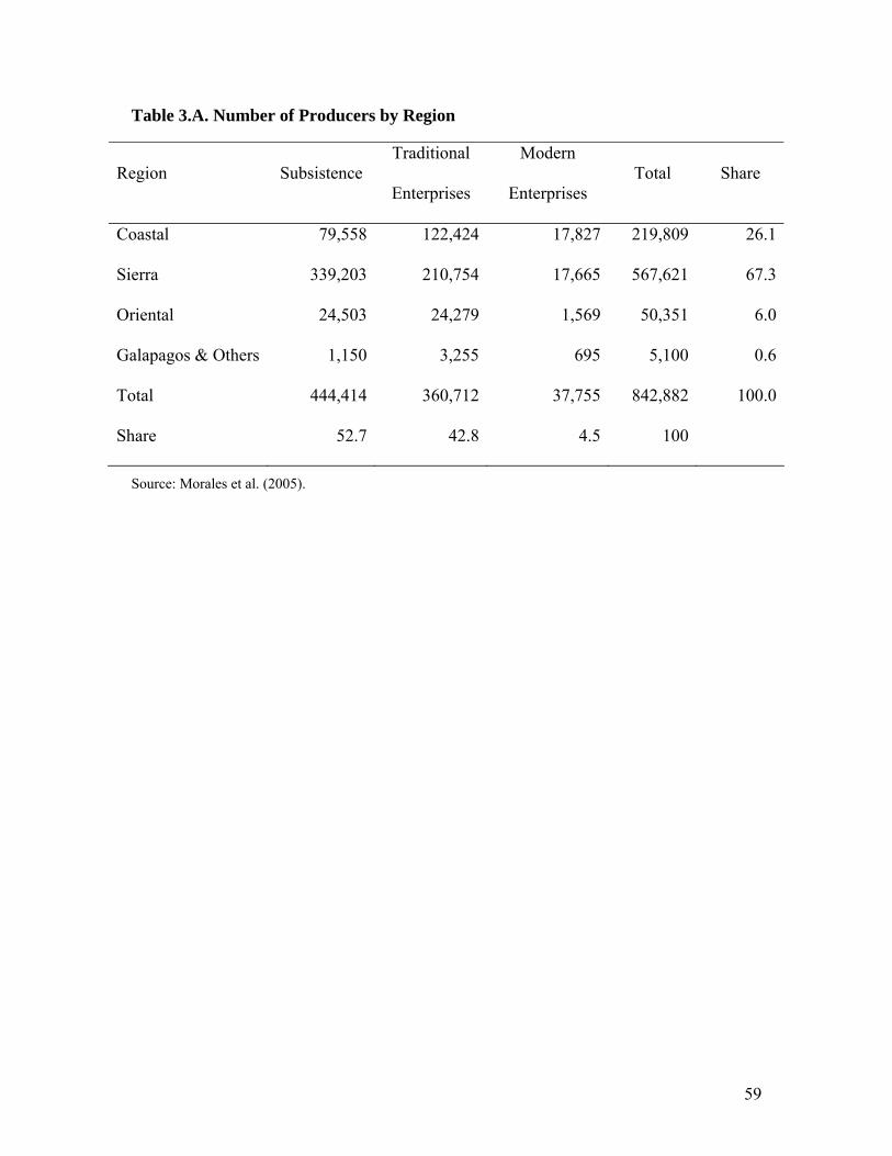
Table 3.A. Number of Producers by Region

Region Subsistence Traditional

Enterprises

Modern

Enterprises Total Share

Coastal 79,558 122,424 17,827 219,809 26.1

Sierra 339,203 210,754 17,665 567,621 67.3

Oriental 24,503 24,279 1,569 50,351 6.0

Galapagos & Others 1,150 3,255 695 5,100 0.6

Total 444,414 360,712 37,755 842,882 100.0

Share 52.7 42.8 4.5 100

Source: Morales et al. (2005).

59

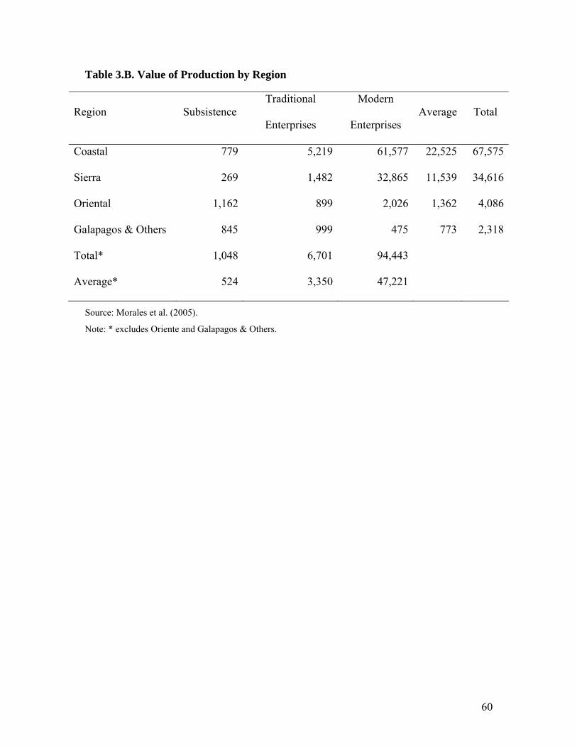
Table 3.B. Value of Production by Region

Region Subsistence Traditional

Enterprises

Modern

Enterprises Average Total

Coastal 779 5,219 61,577 22,525 67,575

Sierra 269 1,482 32,865 11,539 34,616

Oriental 1,162 899 2,026 1,362 4,086

Galapagos & Others 845 999 475 773 2,318

Total* 1,048 6,701 94,443

Average* 524 3,350 47,221

Source: Morales et al. (2005).

Note: * excludes Oriente and Galapagos & Others.

60

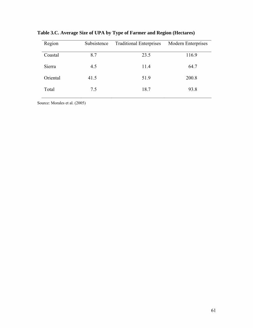
Table 3.C. Average Size of UPA by Type of Farmer and Region (Hectares)

Region Subsistence Traditional Enterprises Modern Enterprises

Coastal 8.7 23.5 116.9

Sierra 4.5 11.4 64.7

Oriental 41.5 51.9 200.8

Total 7.5 18.7 93.8

Source: Morales et al. (2005)

61

Table 3.D. Crop Share of Total Gross Value of Production by Type of Producer

Sierra

Subsistence Traditional Enterprises Modern Enterprises

Dry soft corn 32.6 Potatoes 22.6 Bananas 35.9

Soft corn 2.6 Sugar cane for sugar 21.6 Sugar cane for sugar 17.7

Dry hard corn 3.1 Dry soft corn 12.0 Oil Palm 17.1

Potatoes 18.4 Others 43.8 Potatoes 13.1

Others 43.3 Others 17.1

Total 100.0 Total 100.0 Total 100.0

Coastal

Subsistence Traditional Enterprises Modern Enterprises

Rice 54.1 Rice 36.7 Bananas 71.3

Cacao 13.6 Bananas 22.6 Sugar cane for sugar 8.5

Dry hard corn 12.1 Dry hard corn 12.7 Rice 7.5

Others 20.2 Cacao 7.6 Oil Palm 7.3

Others 20.4 Others 5.4

Total 100.0 Total 100.0 Total 100.0

Source: Morales et al. (2005).

62

63

Table 3.E. Number of UPAs by Type of Producer and Crop

Crop Subsistence Traditional Enterprises Modern Enterprises

Vegetables 303,506 156,241 9,601

Fruits 75,410 101,263 21,947

Corn hard 202,726 126,318 8,055

Corn soft 45,134 23,900 2,220

Paddy Rice 23,725 50,269 5,229

Wheat 19,938 9,946 0

Other Grains 45,683 22,830 1,063

Oil seeds 0 6,824 1,692

Sugar crops 23,236 15,458 1,404

Other crops 79,877 108,634 8,293

Source: Morales et al. (2005)