Geometrical characteristics of magnetospheric energetic ion time series: evidence for low...

Annales Geophysicae (2003) 21: 1975–1993c© European Geosciences Union 2003Annales

Geophysicae

Geometrical characteristics of magnetospheric energetic ion timeseries: evidence for low dimensional chaos

G. P. Pavlos, M. A. Athanasiu, A. G. Rigas, D. V. Sarafopoulos, and E. T. Sarris

Department of Electrical and Computer Engineering, Demokritos Univercity of Thrace, 67100 Xanthi, Greece

Received: 31 October 2002 – Revised: 8 April 2003 – Accepted: 6 May 2003

Abstract. In the first part of the paper we study the geo-metrical characteristics of the magnetospheric ions’ time se-ries in the reconstructed phase space by using the SVD ex-tended chaotic analysis, and we test the strong null hypothe-sis supposing that the ions’ time series is caused by a linearstochastic process perturbed by a static nonlinear distortion.The SVD reconstructed spectrum of the ions’ signal revealsa strong component of high dimensional, external colourednoise, as well as an internal low dimensional nonlinear de-terministic component. Also, the stochastic Lorenz systemproduced by coloured noise perturbation of the deterministicLorenz system was used as an archetype model in compari-son with the dynamics of the magnetrospheric ions.

Key words. Magnetospheric physics (energetic particles) –Radio science (nonlinear phenomena)

1 Introduction

Many theoretical and experimental studies support the hy-pothesis that the magnetosphere can be described as a lowdimensional chaotic system. Theoretically, it was intro-duced by Pavlos (1988, 1994), Baker et al. (1990), Klimaset al. (1991, 1992) and Voros (1991). Experimentally, it wasintroduced by using the chaotic analysis of magnetospherictime series as has been discussed in Vassiliadis et al. (1990,1992), Shan et al. (1991), Roberts et al. (1991), Prichard andPrice (1992), Pavlos et al. (1992a, 1992b, 1994).

Parallel to these studies a fruitful criticism has been devel-oped about the supposition of magnetospheric chaos, espe-cially in relation to its experimental evidence (Prichard andPrice, 1992, 1993; Price and Prichard, 1993; Price et al.,1994; Prichard, 1995), based on the strong null hypothesesfor stochasticity of Theiler (Theiler et al., 1992a, b). Theabove criticism includes the following assertions:

Correspondence to:G. P. Pavlos ([email protected]

(a) The correlation dimension of theAE index time seriescannot be distinguished from that of a stochastic signalwith the same power spectrum and amplitude distribu-tion as the original data.

(b) There is no evidence for the existence of low dimen-sionality according to their estimate of correlation di-mension obtained by using Takens’ method.

(c) There is some evidence for nonlinearity in theAE indextime series. It is not clear whether the nonlinearity of theAE index is the result of the intrinsic dynamics of themagnetosphere or the result of the nonlinearity in thesolar wind.

(d) Because the magnetosphere is largely controlled bythe solar wind, this alone should provide evidenceagainst the existence of a strange attractor in theAE

index, as the magnetosphere is a randomly driven, non-autonomous system.

(e) There is no evidence for low dimensionality of theAE

index and no evidence that theAE index can be de-scribed by a low dimensional strange attractor.

In a recent series of papers, an extended chaotic analysis hasbeen developed by Pavlos et al. (1999a, b, c), Athanasiu andPavlos (2001), in which convincing answers to the above crit-icism against the existence of internal low dimensional andchaotic magnetospheric dynamics have been given. Accord-ing to these papers the magnetospheric chaos hypothesis isstrongly supported by studying the geometrical and dynami-cal characteristics of the magnetospheric time series and theircorresponding nonlinear surrogate data. In these studies amore effective method for constructing surrogate data wasused which was developed by Schreiber and Schmitz (1996)and Schreiber (1998). Also in the last study by Pavlos etal. (1999c), the results of the chaotic analysis of the mag-netospheric time series are compared with corresponding re-sults obtained by analysing different types of stochastic anddeterministic input-output systems. In the same study the

1976 G. P. Pavlos et al.: Geometrical characteristics of magnetospheric energetic ion time series

Energetic Particles (Ions)

-5 -4 -3 -2 -1Log. of Frequency

2

3

4

5

6

7

8

9

10

Log.

of S

pect

ral D

ensi

ty

α

α 1.5D 4

(b)

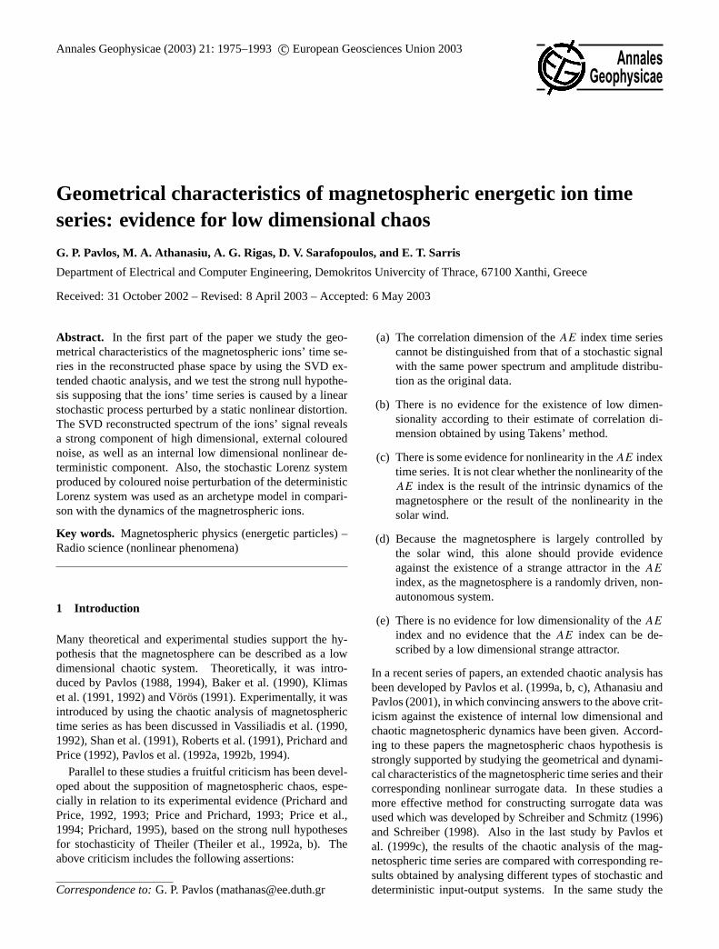
Figure 1 Fig. 1. Power spectrum of the full magnetosphere energetic ions

time series.

spectrum of the SVD reconstructed components of an ex-perimental time series was used as a tool for discriminatingbetween directly external driven and storage-release magne-tospheric processes. Athanasiu and Pavlos (2001) extendedthis concept of the SVD spectrum analysis to the magneto-sphericAE index time series and concluded the existenceof an external, strong, high dimensional, coloured compo-nent in the magnetosphericAE index, which can be discrim-inated by including a low dimensional magnetospheric com-ponent. Similar results supporting the low dimensional mag-netospheric chaos were found by Goode et al. (2001) usingAL index data. For a review of studies concerning magneto-spheric chaos and nonlinear dynamics applied to the Earth’smagnetosphere, refer to Klimas et al. (1996).

In this work the chaotic analysis algorithm is applied forthe study of a new magnetospheric time series correspondingto energetic ions. Some evidence for the low dimensionalchaotic character of this time series was given by Pavloset al. (1999c). Moreover, we extend the study of energeticions time series by examining its geometrical and dynami-cal characteristics. In Sect. 2 we present some theoreticalconcepts and results concerning the background of chaoticanalysis, including the embedding theory, and the method ofSVD analysis. In Sect. 3 we present the results of the chaoticanalysis for the energetic ions’ time series. Finally, in Sect. 4we summarise and discuss the conclusions of this paper.

2 Theoretical framework

The main purpose of time series analysis is to extract signifi-cant information for the underlying dynamics of the observedsignal, as well as to develop effective methods for modellingand prediction. Classical time series analysis confronts theseproblems by using linear or nonlinear input-output methods(Priestley, 1988). On the other hand, the modern analysisof a time series,known as chaotic analysis includes: (a) es-timation of the geometrical and dynamical characteristics of

the trajectory of the system in its phase space (Pavlos et al.,1999a, b; Abarbanel et al., 1993; Grassberger and Procac-cia, 1983; Tsonis, 1992); (b) testing techniques for the dis-crimination of low dimensional, nonlinear determinism andlinear stochastic processes (Provenzale et al., 1992; Theiler,1991; Theiler et al., 1992a, b, 1993); (c) forecasting algo-rithms (Casdagli et al., 1991; Farmer and Sidorowich, 1987;Weigend and Gershenfeld, 1994). The above methods con-stitute the kernel of the chaotic analysis algorithm. This al-gorithm has been enriched recently by new results concern-ing the application of chaotic analysis in known stochasticsystems and input-output systems (Argyris et al., 1998a, b;Pavlos et al., 1999a, b, c), as well as by using the SVD anal-ysis for calculating the spectrum of SVD reconstructed com-ponents of an experimental time series (Elsner and Tsonis,1996; Pavlos et al., 1999c; Athanasiu and Pavlos, 2001).

In the following we summarize the main points of the al-gorithm concerning the chaotic analysis of the experimentalsignals, which will be used in Sect. 3 for the analysis of theenergetic particle signal.

2.1 Classical analysis of time series

The classical theory of time series includes the analysis ei-ther in the time or in the frequency domains (Tong, 1990;Priestley 1988). Both domains are related by the Wiener-Khintchine theorem according to which if the autocorrela-tion function of the signal,C(t), sufficiently decays rapidlyin time, then the power spectrum is equal to the Fourier trans-form of the autocorrelation function and is given by

P(ω) =

∫∞

−∞

C(τ)e−iωτdτ. (1)

In many cases the power spectra of experimental time seriesapproximately follow a power law of the formP(ω) ∼ ω−α.In Fig. 1 the power spectrum of the energetic ions’ time se-ries is presented where it can be seen that the exponenta

takes values in the range (1, 3). In general, with a stochas-tic processx(t), with spectrum density proportional toω−α,it is possible to correspond to a self-affine fractal Brownianmotion (fBm), withH = (α − 1)/2 and fractal dimensionD = 1/H (Osborne and Provenzale, 1989). Because of this,as we show in Sect. 2.7, the Grassberger and Procaccia algo-rithm cannot distinguish between the deterministic chaoticdynamics and a stochastic fractal system (coloured noise),where small space scales are related to small time scales. Itfollows from Eq. (1) that when the power spectrum obeys apower law, then the autocorrelation function decays as thelag timeτ increases. These characteristics can be caused bylinear-nonlinear stochastic dynamical systems or by low di-mensional chaotic dynamical system. Also, the classical timeseries analysis cannot discriminate between these two cases,while the chaotic analysis, as discussed in the following, candiscriminate with high confidence between linear stochastic-ity and low dimensional chaos.

G. P. Pavlos et al.: Geometrical characteristics of magnetospheric energetic ion time series 1977

0 1000 2000 3000 4000 5000t

-30

-20

-10

0

10

20

30

X(t)

Lorenz parameter (e = 0.1) (a)

0 5000 10000 15000 20000 25000 30000 35000t

-15

-10

-5

0

5

10

15

20

X(t)

Lorenz- V1 parameter (e = 0.1) (b)

0 1000 2000 3000 4000 5000t

-15

-10

-5

0

5

10

15

X(t)

Lorenz- V4 parameter (e = 0.1)

(c)

0 5000 10000 15000t

-40

-20

0

20

40

X(t)

Lorenz-(V2-15) parameter (e = 0.1) (d)

-2 -1 0 1 2 3 4Ln(r)

0

1

2

3

4

5

6

7

8

9

10

Slo

pes

Lorenz parameter (e = 0.1)

τ =40m = 5,6,7,8w = 500

(e)

-2 -1 0 1 2 3 4Ln(r)

0

1

2

3

4

5

6

7

8

9

10

Slo

pes

Lorenz-V1 parameter ( e = 0.1)

τ =60m = 5,6,7,8w = 500

(f)

-3 -2 -1 0 1 2 3Ln(r)

0

1

2

3

4

5

6

7

8

9

10

Slo

pes

Lorenz-V4 parameter (e = 0.1)

τ=10m = 5,6,7,8w = 100

(g)

-2 -1 0 1 2 3Ln(r)

0

1

2

3

4

5

6

7

8

9

10

Slo

pes

Lorenz-(V2-15) parameter (e = 0.1)

τ =10m = 5,6,7,8w = 100

(h)

Figure 2 Fig. 2. (a)–(d)The stochastic Lorenz signal corresponding to the coloured noise perturbation 37%(e = 0.1) and its SVD reconstructedcomponentsV1, V4, V2−15. The last signalV2−15 corresponds to the sum

∑Vi , i = 2 − 15. (e)–(h)The slopes of the correlation integrals

estimated for the signals shown in Fig. 2a–d correspondingly, with embeddingm = 5 − 8 andw = 100.

2.2 Embedding theory and phase-space reconstruction

The Earth’s magnetosphere is a system of magnetizedplasma, which microscopically is an infinite dimensionalsystem, the dynamics of which is mirrored in the groundmeasuredAE index or in the energetic particles’ burst ob-served by spacecraft in situ in the magnetosphere or in theinterplanetary space (Pavlos et al., 1999c). Some kind of

“self-organization” may give rise to the system evolution ona low dimensional manifoldM of dimensiond. This meansthat the magnetosphere can be described macroscopically bya low dimensional dynamical system ofn macroscopic de-grees of freedom withn ≥ d. For linear systems, “self-organization” is more an externally driven process describedby the external parameters of the system. For nonlinear anddissipative systems, however, it is possible that the system


0 25 50 75 100 125 150 175 200 225 250Lag(k)

0.0

0.2

0.4

0.6

0.8

1.0

Aut

oc.

Coe

ffici

ent

Lorenz (e=0)

Lorenz-V1 (e=0)

Lorenz (e=0.1)

Lorenz-V1 (e=0.1)

Lorenz (e=0.5)

Lorenz-V1 (e=0.5)

(a)

0 25 50 75 100Lag(k)

-0.4

-0.2

0.0

0.2

0.4

0.6

0.8

1.0

Aut

oc.

Coe

ffici

ent

(b)Lorenz- (V2-15)

e = 0

e = 0.1

e = 0.5

0 25 50 75 100Lag(k)

-0.8

-0.6

-0.4

-0.2

0.0

0.2

0.4

0.6

0.8

1.0

Aut

oc.

Coe

ffici

ent

(c)Lorenz- V4

e = 0

e = 0.1

e = 0.5

Figure 3

Fig. 3. (a) The autocorrelation coefficients of the deterministicx(t) Lorenz signal, of the stochasticx(t) Lorenz signal and itsV1SVD component corresponding to the levelse = 0.1 (37%) ande = 0.5 (185%) of the external additive coloured noise perturbation.(b) The autocorrelation coefficients of theV2−15 SVD componentof the stochasticx(t) Lorenz signal corresponding to the two levelse = 0.1 (37%) ande = 0.5 (185%) of the external additive colourednoise perturbation.(c) The same with Fig. 3b but for theV4 SVDcomponent.

evolves by its internal dynamics in such a way that the cor-responding phase space flow contracts on sets of lower di-mensions which are called attractors. The embedding theorypermits one to study the dynamical characteristics of a phys-ical system by using experimental observations in the formof time series (Takens, 1981; Broomhead and King, 1986).Let x(t) = f (t)(x(0)) denote the dynamical flow underly-ing an experimental time seriesx(ti) = h(x(ti)), whereh

describes the measurement function. When there is a noisycomponentw(ti) then the observed time series must be givenby x(ti) = h(x(ti), w(ti)). On the other hand, Takens (1981)showed that for autonomous and purely deterministic sys-tems, the delay reconstruction map8, which maps the statesx into m-dimensional delay vectors

8(x) = [h(x), h(f τ (x)), h(f 2τ (x)), ..., h(f (m−1)τ (x))] (2)

is an embedding whenm ≥ 2n+1, wheren is the dimensionof the manifoldM of the phase space in which evolves thedynamics of the system. This means that interesting geomet-rical and dynamical characteristics of the underlying dynam-ics in the original phase space are preserved invariably in thereconstructed space as well.

Let Xr = 8(t)(X) be the reconstructed phase space andxr(ti) = 8(x(ti)) the reconstructed trajectory for the em-bedding8. Then the dynamics evolved in the original phasespace is topologically equivalent to its mirror dynamical flowin the reconstructed phase spaceXr according to

f tr (xr) = 8(x) ◦ f t (x) ◦ 8−1(xr). (3)

In other words, the embedding8 is a diffeomorphism whichtakes the orbitsf t (xr) of the original phase space to theorbits in the reconstructed phase in such a way as to pre-serve their orientation and other topological characteristicsas eigenvalues, Lyapunov exponents or dimensions of the at-tractors. According to the above theory, in the reconstructedphase space we can estimate geometrical characteristics asdimensions, which correspond to the degrees of freedom ofthe underlying dynamics of the experimental time series, aswell as dynamical characteristics as Lyapunov exponents,mutual information and predictors (Pavlos et al., 1999a, b).Moreover, it is shown elsewhere that the method of recon-structed phase space conserves its significance even when theobserved signal is derived by a stochastic process (Argyris etal., 1998; Pavlos et al., 1999c).

2.3 Correlation dimension

The theoretical concepts described above permit us to useexperimental time series in order to extract useful geomet-ric characteristics, which provide information about the un-derlying dynamics. Such a characteristic is the correlationdimensionD, defined as

D = limr→0

d[ln C(r)]

d[ln(r)], (4)

whereC(r) is the so-called correlation integral for a radiusr in the reconstructed phase space. When an attracting setexists, thenC(r) reveals a scaling profile

C(r) ∼ rd for r → 0. (5)

The correlation integral depends on the embedding dimen-sionm of the reconstructed phase space and is given by thefollowing relation

C(r, m) =2

N(N − 1)

N∑i=1

N∑j=i+1

2(r− ‖ x(i) − x(j) ‖), (6)


0 5 10 15 20 25 30 35 40i

0.0

0.2

0.4

0.6

0.8

1.0

1.2

Lorenz, (e = 0)

Lorenz, (e = 0.1)

Lorenz-V1, (e = 0.1)

Lorenz-(V2-15), (e = 0.1)

(a)

0 5 10 15 20 25 30 35 40i

0.0

0.2

0.4

0.6

0.8

1.0

1.2

Lorenz, (e = 0)

Lorenz, (e = 0.5)

Lorenz-V1, (e = 0.5)

Lorenz-(V2-15), (e = 0.5)

(b)

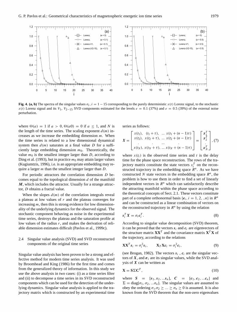
Figure 4 Fig. 4. (a, b)The spectra of the singular valuesσi , i = 1− 15 corresponding to the purely deterministicx(t) Lorenz signal, to the stochasticx(t) Lorenz signal and itsV1, V2−15 SVD components estimated for the levelse = 0.1 (37%) ande = 0.5 (39%) of the external noiseperturbation.

where2(a) = 1 if a > 0, 2(a0) = 0 if a ≤ 1, andN isthe length of the time series. The scaling exponentd(m) in-creases as we increase the embedding dimensionm. Whenthe time series is related to a low dimensional dynamicalsystem thend(m) saturates at a final valueD for a suffi-ciently large embedding dimensionm0. Theoretically, thevaluem0 is the smallest integer larger thanD, according toDing et al. (1993), but in practicem0 may attain larger values(Kugiumtzis, 1996), i.e. is an appropriate embedding may re-quire a largerm than the smallest integer larger thanD.

For periodic attractors the correlation dimensionD be-comes equal to the topological dimensiond of the manifoldM, which includes the attractor. Usually for a strange attrac-tor, D obtains a fractal value.

When the slopesd(m) of the correlation integrals reveala plateau at low values ofr and the plateau converges forincreasingm, then this is strong evidence for low dimension-ality of the underlying dynamics for the observed signal. Thestochastic component behaving as noise in the experimentaltime series, destroys the plateau and the saturation profile atlow values of the radiusr, and makes the derivation of reli-able dimension estimates difficult (Pavlos et al., 1999c).

2.4 Singular value analysis (SVD) and SVD reconstructedcomponents of the original time series

Singular value analysis has been proven to be a strong and ef-fective method for modern time series analysis. It was usedby Broomhead and King (1986) for the first time and comesfrom the generalized theory of information. In this study weuse the above analysis in two cases: (i) as a time series filterand (ii) to decompose a time series in its SVD reconstructedcomponents which can be used for the detection of the under-lying dynamics. Singular value analysis is applied to the tra-jectory matrix which is constructed by an experimental time

series as follows:

X =

x(t1), (t1 + τ), ... x(t1 + (n − 1)τ )

x(t2), x(t2 + τ), ... x(t2 + (n − 1)τ )

. . ... .

x(tN ), x(tN + τ), ... x(tN + (n − 1)τ )

=

xT

1xT

2.

xTN

, (7)

wherex(ti) is the observed time series andt is the delaytime for the phase space reconstruction. The rows of the tra-jectory matrix constitute the state vectorsxT

i on the recon-structed trajectory in the embedding spaceRn. As we haveconstructedN state vectors in the embedding spaceRn, theproblem is how to use them in order to find a set of linearlyindependent vectors inRn which can satisfactorily describethe attracting manifold within the phase space according tothe theoretical concepts of Sect. 2.1. These vectors constitutepart of a complete orthonormal basis{ei, i = 1, 2, ..n} in Rn

and can be constructed as a linear combination of vectors onthe reconstructed trajectory inRn by using the relation

sTi X = σic

Ti . (8)

According to singular value decomposition (SVD) theorem,it can be proved that the vectorssi andci are eigenvectors ofthe structure matrixXXT and the covariance matrixXT X ofthe trajectory, according to the relations

XXT si = σ 2i si, XT Xci = σ 2

i ci, (9)

(see Brogan, 1982). The vectorssi , ci are the singular vec-tors ofX, andσ i are its singular values, while the SVD anal-ysis ofX can be written as

X = S6CT , (10)

where S = [s1, s2, ...sn], C = [c1, c2, ...cn] and6 = diag[σ1, σ2, ...σn]. The singular values are assumed toobey the orderingσ≥σ2 ≥ ... ≥ σn ≥ 0 is assumed. It is alsoknown from the SVD theorem that the non-zero eigenvalues


of the structure matrix are equal the to non-zero eigenval-ues of the covariance matrix. This means that ifn′ (wheren′

≥ n) is the number of the non-zero eigenvalues, thenrankXXT

= rankXT X = n′. It is obvious that the n′-dimensional subspace ofRN spanned by{si, i = 1, 2, ...n′

}

is mirrored to the basis vectorci , which can be found as thelinear combination of the delay vectors by using the eigen-vectorssi according to Eq. (8). The complementary subspacespanned by the set{si, i = n′, 2, ...N} is mirrored to the ori-gin of the embedding spaceRn according to the same relation(8) i.e. the number of the independent eigenvectorsci thatare sufficient for the description of the underlying dynamicsis equal to the numbern′ of the non-zero singular valuesσi

of the trajectory matrix. The same numbern′ corresponds tothe dimensionality of the subspace containing the attractingmanifold. The trajectory can be described on the new basis{ci, i = 1, 2, ...n} by the trajectory matrix projected on thebasis{ci} given by the productXC of the old trajectory ma-trix X and the matrixC of the eigenvectors{ci}. The newtrajectory matrixXC is described by the relation

(XC)T (XC) = 62. (11)

This relation corresponds to the diagonalization of the newcovariance matrix so that the components of the trajectoryare uncorrelated in the basis{ci}. Also, from the same re-lation (11) we conclude that each eigenvalueσ 2

i is the meansquare projection of the trajectory on the correspondingci .Thus, the spectrum{σ 2

i } includes information about the ex-pansion of the trajectory in the directionsci as it evolves inthe reconstructed phase space. This phase space, exploredby the trajectory, corresponds – on the average – to ann-dimensional ellipsoid for which{ci} give the directions and{σ i} the lengths of its principal axes in the subspace spannedby eigenvectors{ci} corresponding to non-zero eigenvalues.However, when the system is perturbed by external noiseor deterministic external input, then the trajectory begins tobe diffused in directions corresponding to zero eigenvalueswhere the external perturbation dominates. As we show inthe following, the replacement of the old trajectory matrixX with the newXC works as a linear low pass filter for theentire trajectory. Moreover, the SVD analysis permits oneto reconstruct the original trajectory matrix by using theXCmatrix as follows

X =

n∑i=1

(Xci)cTi . (12)

The part of the trajectory matrix which contains all theinformation about the deterministic trajectory, as it can beextracted by observations, corresponds to the reduced matrix

X =

n′∑i=1

(Xci)cTi , (13)

which is obtained by summing only with respect to eigenvec-torsci with non-zero eigenvalues. From the relation (12) we

Figure 5

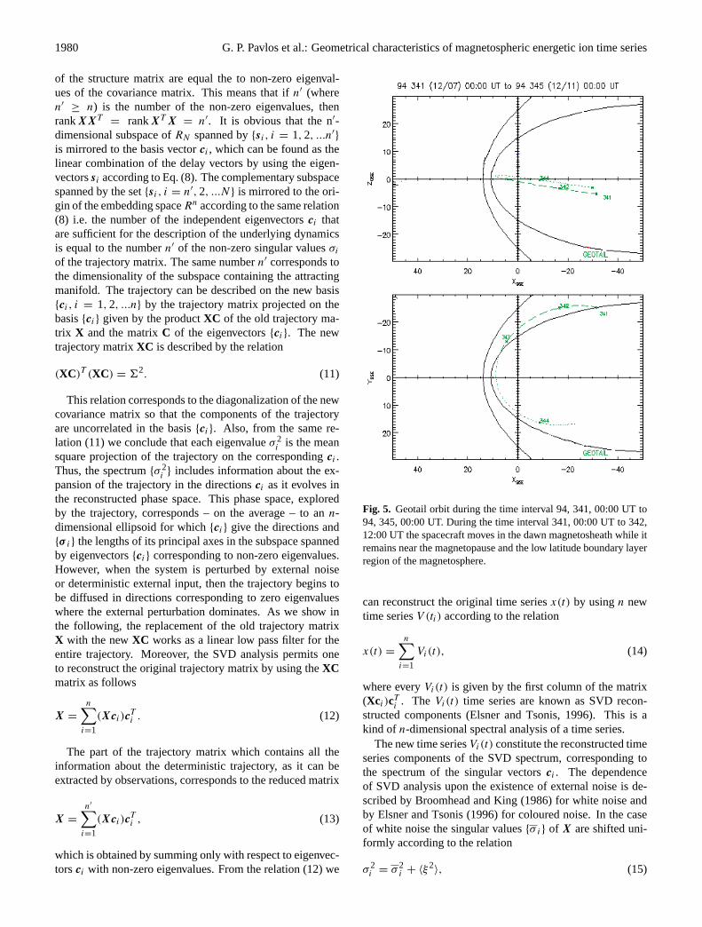
Fig. 5. Geotail orbit during the time interval 94, 341, 00:00 UT to94, 345, 00:00 UT. During the time interval 341, 00:00 UT to 342,12:00 UT the spacecraft moves in the dawn magnetosheath while itremains near the magnetopause and the low latitude boundary layerregion of the magnetosphere.

can reconstruct the original time seriesx(t) by usingn newtime seriesV (ti) according to the relation

x(t) =

n∑i=1

Vi(t), (14)

where everyVi(t) is given by the first column of the matrix(Xci)cT

i . The Vi(t) time series are known as SVD recon-structed components (Elsner and Tsonis, 1996). This is akind of n-dimensional spectral analysis of a time series.

The new time seriesVi(t) constitute the reconstructed timeseries components of the SVD spectrum, corresponding tothe spectrum of the singular vectorsci . The dependenceof SVD analysis upon the existence of external noise is de-scribed by Broomhead and King (1986) for white noise andby Elsner and Tsonis (1996) for coloured noise. In the caseof white noise the singular values{σ i} of X are shifted uni-formly according to the relation

σ 2i = σ 2

i + 〈ξ2〉, (15)


0

0.4

0.8

1.2

1.6

O+ /

H+

0

2000

4000

6000

elet

rons

flux

es

EPIC/ICS> 38 keV

0 40000 80000 120000 160000

-60-40-20

0204060

B z (n

T)

(b)

(c)

(d)

(a)

EPIC/STICS7.5 - 230 keV

AE

Day 341 Day 342

Day 341 Day 342

UT (sec)

Day 342

Day 342

Day 341

UT (hours)

Day 341

Year 1994

AO

Figure 6 Fig. 6. From top to bottom,(a) AE index measurements with one minute resolution,(b) the energetic>38 keV electrons (second panel),(c)the ratio O+/H+ (third panel) and(d) theBz component (fourth panel).

whereσ i are the singular values of the unperturbed signaland〈ξ2

〉 the perturbation of the external noise. Relation (15)indicates that, in the simple case of white noise the existenceof a non-zero constant background or noise floor in the spec-trum{σ1} can be used to distinguish the deterministic compo-nent. In this way we can obtain the deterministic componentof the observed time series

Xd =

∑σi 〉noise

((Xc)i)cTi (16)

by using only singular valuesσi greater than the noise floor.In addition, the relation (15) indicates that in the case ofwhite noise the perturbation of the singular valuesσi is in-dependent of them. In contrast, as we show in the fol-lowing, in the case of coloured noise the perturbation ofthe singular values is much stronger for the first singularvalue {σ1} than the others. This result may be expected as

the coloured noise includes finite dimensional determinismwhile the white noise includes an infinite dimensional sig-nal. The above difference between white and coloured noiseis significant because it makes the SVD analysis suitable forthe discrimination between different dynamical componentsof the original signal.

2.5 Application of the SVD analysis in the deterministicand stochastic Lorenz system

In this section we apply the SVD analysis at the Lorenz sys-tem perturbed by external additive colored noise. The exter-nal colored noise is obtained by the equation

X(ti) =

M/2∑k=1

Ck cos(ωkti + ϕk), i = 1, ..., M, (17)


0 5000 10000 15000 20000t(X6sec)

0

200

400

600

800

Ions

(a)Energetic Ions

0 200 400 600 800 1000 1200 1400Lag(k)

-0.2

0.0

0.2

0.4

0.6

0.8

1.0

Auto

c. C

oeffi

cien

t

Energetic Ions (b)

Energetic Particles (Ions)

-2 -1 0 1 2 3X

0.00

0.05

0.10

0.15

Den

sity

P(

X)

First halfSecond half

(c)

Figure 7

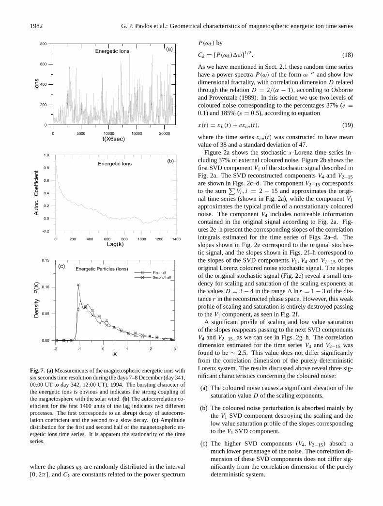
Fig. 7. (a)Measurements of the magnetospheric energetic ions withsix seconds time resolution during the days 7–8 December (day 341,00:00 UT to day 342, 12:00 UT), 1994. The bursting character ofthe energetic ions is obvious and indicates the strong coupling ofthe magnetosphere with the solar wind.(b) The autocorrelation co-efficient for the first 1400 units of the lag indicates two differentprocesses. The first corresponds to an abrupt decay of autocorre-lation coefficient and the second to a slow decay.(c) Amplitudedistribution for the first and second half of the magnetospheric en-ergetic ions time series. It is apparent the stationarity of the timeseries.

where the phasesϕk are randomly distributed in the interval[0, 2π], andCk are constants related to the power spectrum

P(ωk) by

Ck = [P(ωk)1ω]1/2. (18)

As we have mentioned in Sect. 2.1 these random time serieshave a power spectraP(ω) of the formω−α and show lowdimensional fractality, with correlation dimensionD relatedthrough the relationD = 2/(α − 1), according to Osborneand Provenzale (1989). In this section we use two levels ofcoloured noise corresponding to the percentages 37% (e =

0.1) and 185% (e = 0.5), according to equation

x(t) = xL(t) + excn(t), (19)

where the time seriesxcn(t) was constructed to have meanvalue of 38 and a standard deviation of 47.

Figure 2a shows the stochasticx-Lorenz time series in-cluding 37% of external coloured noise. Figure 2b shows thefirst SVD componentV1 of the stochastic signal described inFig. 2a. The SVD reconstructed componentsV4 andV2−15are shown in Figs. 2c–d. The componentV2−15 correspondsto the sum

∑Vi, i = 2 − 15 and approximates the origi-

nal time series (shown in Fig. 2a), while the componentV1approximates the typical profile of a nonstationary colourednoise. The componentV4 includes noticeable informationcontained in the original signal according to Fig. 2a. Fig-ures 2e–h present the corresponding slopes of the correlationintegrals estimated for the time series of Figs. 2a–d. Theslopes shown in Fig. 2e correspond to the original stochas-tic signal, and the slopes shown in Figs. 2f–h correspond tothe slopes of the SVD componentsV1, V4 andV2−15 of theoriginal Lorenz coloured noise stochastic signal. The slopesof the original stochastic signal (Fig. 2e) reveal a small ten-dency for scaling and saturation of the scaling exponents atthe valuesD = 3 − 4 in the range1 ln r = 1 − 3 of the dis-tancer in the reconstructed phase space. However, this weakprofile of scaling and saturation is entirely destroyed passingto theV1 component, as seen in Fig. 2f.

A significant profile of scaling and low value saturationof the slopes reappears passing to the next SVD componentsV4 andV2−15, as we can see in Figs. 2g–h. The correlationdimension estimated for the time seriesV4 andV2−15 wasfound to be∼ 2.5. This value does not differ significantlyfrom the correlation dimension of the purely deterministicLorenz system. The results discussed above reveal three sig-nificant characteristics concerning the coloured noise:

(a) The coloured noise causes a significant elevation of thesaturation valueD of the scaling exponents.

(b) The coloured noise perturbation is absorbed mainly bytheV1 SVD component destroying the scaling and thelow value saturation profile of the slopes correspondingto theV1 SVD component.

(c) The higher SVD components(V4, V2−15) absorb amuch lower percentage of the noise. The correlation di-mension of these SVD components does not differ sig-nificantly from the correlation dimension of the purelydeterministic system.


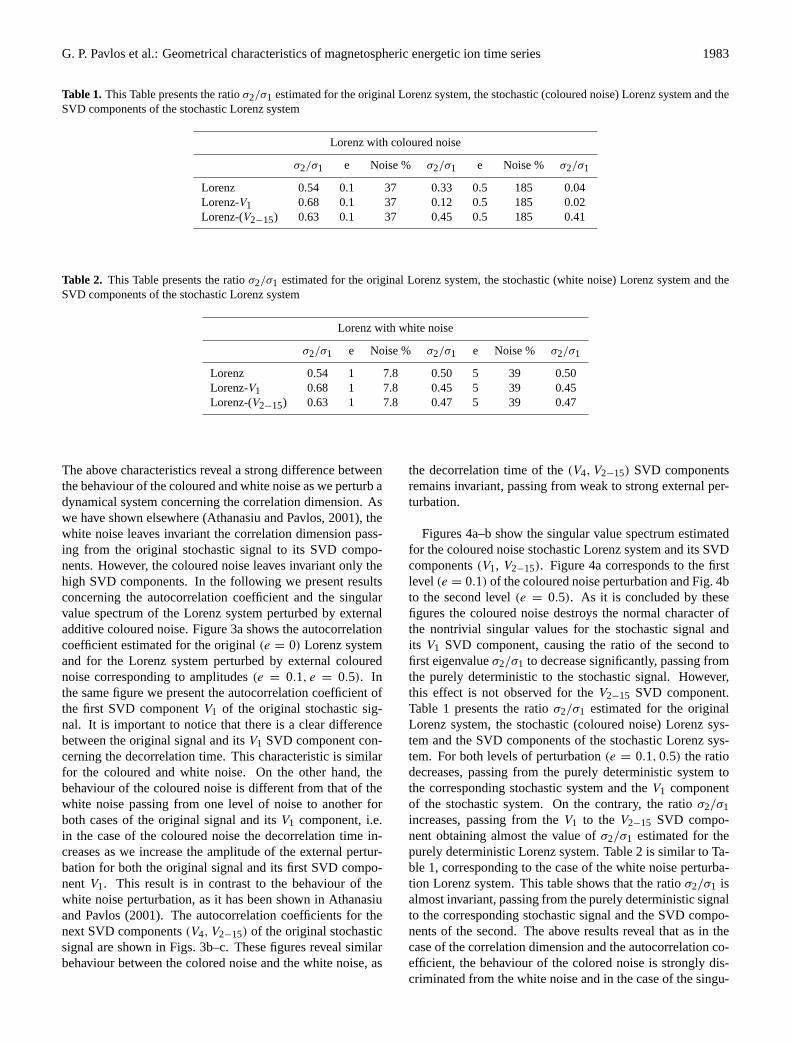
Table 1. This Table presents the ratioσ2/σ1 estimated for the original Lorenz system, the stochastic (coloured noise) Lorenz system and theSVD components of the stochastic Lorenz system

Lorenz with coloured noise

σ2/σ1 e Noise % σ2/σ1 e Noise % σ2/σ1

Lorenz 0.54 0.1 37 0.33 0.5 185 0.04Lorenz-V1 0.68 0.1 37 0.12 0.5 185 0.02Lorenz-(V2−15) 0.63 0.1 37 0.45 0.5 185 0.41

Table 2. This Table presents the ratioσ2/σ1 estimated for the original Lorenz system, the stochastic (white noise) Lorenz system and theSVD components of the stochastic Lorenz system

Lorenz with white noise

σ2/σ1 e Noise % σ2/σ1 e Noise % σ2/σ1

Lorenz 0.54 1 7.8 0.50 5 39 0.50Lorenz-V1 0.68 1 7.8 0.45 5 39 0.45Lorenz-(V2−15) 0.63 1 7.8 0.47 5 39 0.47

The above characteristics reveal a strong difference betweenthe behaviour of the coloured and white noise as we perturb adynamical system concerning the correlation dimension. Aswe have shown elsewhere (Athanasiu and Pavlos, 2001), thewhite noise leaves invariant the correlation dimension pass-ing from the original stochastic signal to its SVD compo-nents. However, the coloured noise leaves invariant only thehigh SVD components. In the following we present resultsconcerning the autocorrelation coefficient and the singularvalue spectrum of the Lorenz system perturbed by externaladditive coloured noise. Figure 3a shows the autocorrelationcoefficient estimated for the original(e = 0) Lorenz systemand for the Lorenz system perturbed by external colourednoise corresponding to amplitudes(e = 0.1, e = 0.5). Inthe same figure we present the autocorrelation coefficient ofthe first SVD componentV1 of the original stochastic sig-nal. It is important to notice that there is a clear differencebetween the original signal and itsV1 SVD component con-cerning the decorrelation time. This characteristic is similarfor the coloured and white noise. On the other hand, thebehaviour of the coloured noise is different from that of thewhite noise passing from one level of noise to another forboth cases of the original signal and itsV1 component, i.e.in the case of the coloured noise the decorrelation time in-creases as we increase the amplitude of the external pertur-bation for both the original signal and its first SVD compo-nent V1. This result is in contrast to the behaviour of thewhite noise perturbation, as it has been shown in Athanasiuand Pavlos (2001). The autocorrelation coefficients for thenext SVD components(V4, V2−15) of the original stochasticsignal are shown in Figs. 3b–c. These figures reveal similarbehaviour between the colored noise and the white noise, as

the decorrelation time of the(V4, V2−15) SVD componentsremains invariant, passing from weak to strong external per-turbation.

Figures 4a–b show the singular value spectrum estimatedfor the coloured noise stochastic Lorenz system and its SVDcomponents(V1, V2−15). Figure 4a corresponds to the firstlevel(e = 0.1) of the coloured noise perturbation and Fig. 4bto the second level(e = 0.5). As it is concluded by thesefigures the coloured noise destroys the normal character ofthe nontrivial singular values for the stochastic signal andits V1 SVD component, causing the ratio of the second tofirst eigenvalueσ2/σ1 to decrease significantly, passing fromthe purely deterministic to the stochastic signal. However,this effect is not observed for theV2−15 SVD component.Table 1 presents the ratioσ2/σ1 estimated for the originalLorenz system, the stochastic (coloured noise) Lorenz sys-tem and the SVD components of the stochastic Lorenz sys-tem. For both levels of perturbation(e = 0.1, 0.5) the ratiodecreases, passing from the purely deterministic system tothe corresponding stochastic system and theV1 componentof the stochastic system. On the contrary, the ratioσ2/σ1increases, passing from theV1 to the V2−15 SVD compo-nent obtaining almost the value ofσ2/σ1 estimated for thepurely deterministic Lorenz system. Table 2 is similar to Ta-ble 1, corresponding to the case of the white noise perturba-tion Lorenz system. This table shows that the ratioσ2/σ1 isalmost invariant, passing from the purely deterministic signalto the corresponding stochastic signal and the SVD compo-nents of the second. The above results reveal that as in thecase of the correlation dimension and the autocorrelation co-efficient, the behaviour of the colored noise is strongly dis-criminated from the white noise and in the case of the singu-


1.0 1.5 2.0 2.5 3.0 3.5 4.0 4.5 5.0 5.5Ln(r)

0

1

2

3

4

5

6

7

8

9

10S

lope

sEnergetic Ions(a)

τ = 10 w = 50

τ = 20 w = 50

τ = 30 w = 50

τ = 40 w = 50

τ = 50 w = 50

τ = 70 w = 100

τ = 100 w = 100

m = 6

0.5 1.0 1.5 2.0 2.5 3.0 3.5 4.0 4.5 5.0 5.5Ln(r)

0

1

2

3

4

5

6

7

8

Slo

pes

Energetic Ions τ=30w=50

m=4

m=5

m=6

m=7

(c)

1.0 1.5 2.0 2.5 3.0 3.5 4.0 4.5 5.0 5.5Ln(r)

0

1

2

3

4

5

6

7

8

Slo

pes

Energetic Ions(b) m = 6

τ = 30

w=50

w=100

w=500

1.5 2.0 2.5 3.0 3.5 4.0 4.5 5.0Ln(r)

0

1

2

3

4

5

6

7

8

Slo

pes

tw=40

m=5, τ=8

m=6 , τ=7

m=7 , τ=6

m=8 , τ=5

Energetic ions(d)

Figure 8 Fig. 8. (a)The slope of the correlation integral as a function of the radiusr estimated for embeddingm = 6, delay timeτ = 10− 100 unitsof the sampling time and Theiler’s parameterw = 50, 100. For delay timeτ = 20− 50 we observe the best scaling.(b) The same as (a) butwith delayτ = 30 andw = 5500, showing that there is no significant change of the slopes.(c) The same as (a) but withτ = 30,w = 500and a embedding dimensionm = 4 − 7. (d) The same as (c) estimated by using the SVD filtering of the original signal for window lengthτw, w = 50 and independent trajectory matrices for every embedding.

lar value spectrum as well.

2.6 The method of the false nearest neighbours in the esti-mation of the dynamical degrees of freedom

Besides the correlation dimension, the method of false near-est neighbours can also give an estimation of the small-est value that is appropriate for the embedding dimensionm0. When the trajectory of the system is reconstructed ina space of low dimensionality, then it is possible to haveself-crossings which give rise to false neighbours state vec-tors. This is gradually improved as the embedding dimensionis increased, and for a large enough embedding dimensionm0 false crossings and false neighbours disappear. Letx(j)

be the nearest point tox(i) for an embedding dimensionm.Then their distance is given by

r2m(i, j) =

[x(i)−x(j)]2+...+[x(i+(m−1)τ )−x(j +(m−1)τ ]2.(20)

Passing from them to m + 1 embedding dimension thisdistance takes the form

r2m+1(i, j) = r2

m(i, j) + [x(i + mτ) − x(j + mτ)]2. (21)

Then if|x(i + mτ) − x(j + mτ)|

rm> RT , (22)

the nearest neighbours at timei are declared as false (Abar-banel et al., 1993). The threshold valueRT is estimated tobe in the range 10≤ RT ≤ 50. According to this criterion,as the embedding dimensionm increases to a characteristicvaluem0, the percent of false nearest neighbours may dropto zero. If this is actually observed for a time series, thenit yields a positive indication of the existence of low dimen-sional dynamics underlying the observed signal.

2.7 The method of surrogate data

According to the relation (5), the scaling properties of thecorrelation integral asr → 0 and the saturation of the scal-ing exponentd(m) → D asm increases are necessary con-ditions for the existence of low dimensional dynamics un-derlying the experimental time series. However, it has beenshown that these conditions are not sufficient in order to con-clude low dimensional dynamics from experimental time se-ries with broad-band power spectrum, as they can also be sat-isfied by stochastic systems (Osborne and Provenzale, 1989;


1.0 1.5 2.0 2.5 3.0 3.5 4.0 4.5 5.0 5.5Ln(r)

0

1

2

3

4

5

6

7

8S

lope

s(a)

m =6t = 30w =100

Energetic Ions

Surrogates

1.5 2.0 2.5 3.0 3.5 4.0 4.5 5.0Ln(r)

0

1

2

3

4

5

6

7

8

Slo

pes

SVD filter

Energetic Ions

Surrogates

m = 6τ = 7w = 100

(c)

2 3 4 5 6ln(r)

0

2

4

6

Sig

mas

Surrogates m = 6τ = 30w = 100

(b)

2.5 3.0 3.5 4.0 4.5 5.0Ln(r)

0

1

2

3

4

5

6

7

8

9

10

Sig

mas

m = 6τ = 7w=100

SVD filterSurrogates

(d)

Figure 9 Fig. 9. (a)Slopes of the correlation integrals estimated for the original signal and its first 30 surrogate data as a function of ln(r). (b) Thesignificance of the statistics as a function of ln(r), shown in (a).(c, d) The same as (a, b) but SVD analysis was used.

Provenzale et al., 1991). Moreover, according to Theiler(1991), the concept of low correlation dimension (fractal orinteger) can be applied to time series in two distinct ways.The first one indicates the number of degrees of freedom inthe underlying dynamics, and the second quantifies the self-affinity or “crinkliness” of the trajectory through the phasespace. In the first case, the scaling and saturation profile arecaused by the recurrent character of the reconstructed trajec-tory, i.e. by uncorrelated in “time” and correlated in “space”state points. In the second case, they are caused by time cor-related state points that are uncorrelated in space. In order todiscriminate between the two cases, known as dynamic andgeometric low dimensionality, we restrict the sum in Eq. (6)to pairs(x(i), x(j)) with |i − j | > w, where the Theilerparameterw is larger than the decorrelation time of the timeseries.

When low dimensionality is persistent as a dynamiccharacteristic after the application of Theiler’s criterion, thenwe have to decide first between linearity and nonlinearityand second between chaoticity and pure stochasticity. Bythe term chaoticity we mean the case where the deterministiccomponent of the process is prevalent and reveals low di-mensional chaos. For a stochastic process, the deterministiccomponent may correspond to low dimensionality and even

nonlinear and chaotic dynamics, but its effect can hardly beobserved as the process is driven mainly by noise. There-fore, we focus here on the solution of the first problem, i.e.determining whether the magnetospheric ions’ time series islinear or nonlinear. This is done by following the method of“surrogate” data (Theiler et al., 1992a, b).

The method of “surrogate” data includes the generation ofan ensemble of data sets which are consistent to a null hy-pothesis. According to Theiler (1992a), the first type of nullhypothesis is the linearly correlated noise which mimics theoriginal time series in terms of the autocorrelation function,variance and mean. The second and more general null hy-pothesis takes into account that the observed time series maybe a nonlinear monotonic static distortion of a stochastic sig-nal.

Every Gaussian process is linear, while a non-Gaussianprocess can be linear or nonlinear. An experimental time se-ries may show nonlinearity in terms of a non-Gaussian dis-tribution, which may be due to a nonlinear transformationof the linear underlying dynamics. In this case, the generated“nonlinear” surrogate data mimic the original time seriesx(i)

in terms of the autocorrelation function and the probabilitydensity functionp(x). It is always possible for a nonperiodictime series of finite length to be a particular realisation of a


noise process or of a low-dimensional deterministic process.Therefore, it is a statistical problem to distinguish betweena nonlinear deterministic process and a linear stochastic pro-cess. For this purpose we use as discriminating statistic aquantity Q derived by a method sensitive to nonlinearity,as the correlation dimension estimation. The discriminat-ing statisticQ is calculated for the original and the surrogatedata, and the null hypothesis is verified or rejected accordingto the value of “sigmas”S

S =µobs − µsur

σsur

, (23)

whereµsur andσsur is the mean and the standard deviationof Q on the surrogate data, andµobs is the mean ofQ on theoriginal data. For a single time series,µobs is the singleQvalue (Theiler et al., 1992a).

The significance of the statistics is a dimensionless quan-tity, but we follow here the common parlance and report it interms of the units ofS “sigmas”. WhenS takes values higherthan 2–3, then the probability that the observed time seriesdoes not belong to the same family with its surrogate data ishigher than 0.95–0.99, correspondingly.

For testing the second more general null hypothesisdescribed above we follow Theiler’s algorithm (Theiler,1992a), as well as Schreiber and Schmitz’s algorithm(Schreiber and Schmitz, 1996). Both algorithms createstochastic signals which have the same autocorrelation func-tion and amplitude distribution as the original time series.

According to Theiler’s algorithm, a white Gaussian noiseis first reordered to match the rank of the original time series(this is to make the original time series Gaussian). Then thephases of this signal are randomized (to destroy any possiblenonlinear structure). Finally, the original signal is reorderedto match the rank of the above constructed coloured noise(to regain the original amplitude distribution). The derivedshuffled time series is the surrogate time series.

The algorithm of Theiler was improved by Schreiber andSchmitz by a simple iteration scheme, in order to strengthenthe ability of the surrogate data to fit more exactly the auto-correlation function and the power spectrum of the originaltime series. The procedure starts with a white noise signal, inwhich the Fourier amplitudes are replaced by the correspond-ing amplitudes of the original data. The rank order of thederived stochastic signal is used to reorder the original timeseries. By doing this the matching of amplitude distributionis succeeded, but the matching of power spectrum achievedin the first step is altered. Therefore, the process obtainedin the two steps is repeated several times until the change inthe matching of power spectrum is sufficiently small. In theanalysis of our data the improved algorithm of Schreiber andSchmitz is used.

3 Data analysis and results

It is known that protons or heavy ions as O6+ could be ac-celerated by Fermi acceleration at the Earth’s bow shock

(Ipavich et al., 1981; Freeman and Parks, 2000). However,low charge state heavy ions are thought to be coming fromthe Earth’s ionosphere and accelerated in the magnetotail(Kirsch et al., 1984; Pavlos et al., 1985; Eastman and Chris-ton, 1995; Anagnostopoulos et al., 1986, 1998; Sarafopouloset al., 1999; Christon et al., 2000). Moreover, it is knownthat bursts of energetic electrons are caused only by acceler-ation in the Earth’s magnetotail (Pavlos et al., 1985; Anag-nostopoulos et al., 1986; Sarafopoulos et al., 2000). In thiswork we study an extendend time series of energetic ions asthey were observed at the dawn magnetosheath of the Earth’smagnetopshere. As we can see in Figs. 5a–b during the days7–8 December (days 341–342), 1994, the spacecraft GEO-TAIL moves in the down magnetosheath while it remainsnear the magnetopause and the low-latitude boundary layer(LLBL) region of the magnetosphere. Figure 6a shows theAE index during the same period. The profile of theAE

index indicates strong magnetopsheric activity which couldcause the acceleration of electrons, protons and low chargestate heavy ions as O6+. Figures 6b–c present energetic elec-tron fluxes as well as O+ fluxes, which obviously were ac-celerated at the Earth’s magnetotail. Figure 6d shows theBz

magnetic field measurements during the same period. TheBz component changes continuously from negative to posi-tive values, indicating the magnetic connection of the space-craft’s position and the Earth’s magnetosphere. The magneticconnection of the spacecraft and magnetopshere can be alsoconcluded by the existence of energetic electron bursts (seeFig. 6b). Sarafopoulos et al. have also determined energeticelectrons and proton bursts during the same period, and theyconcluded their magnetopsheric origin (Sarafopoulos et al.,2000). These observations strongly support the hypothesisthat the energetic ions observed during the same period atthe dawn magnetosheath were produced at the Earth’s mag-netotail.

Figure 7a shows the measurements of the energetic ions(35–46.8 keV) as they were observed by the experimentEPIC/ICS during the days 7–8 December (day 341, 00:00 UTto day 342, 12:00 UT), 1994, at the dawn magnetosheathof the Earth’s magnetosphere. This figure reveals strongand continuously repeatable bursts of energetic ions during∼36 h. As it was explained before, it is reasonable to sup-pose that these particles were accelerated in the inner mag-netosphere during periods with a strong coupling of the mag-netospheric system and the solar wind, simultaneously withstrong bursts of electrons and O+, as well as a clear en-hancement of theAE index. Therefore, it can be supposedthat the dynamics of the energetic ions mirror the internalmagnetospheric dynamics, similar to theAE index duringperiods with a strong coupling of the magnetosphere andthe solar wind (Pavlos et al., 1999c). The energetic parti-cle differential fluxes are provided via the Energetic Parti-cle and Ion Composition (EPIC) instrument of the GEOTAILspacecraft,and essentially remained close to the ecliptic plane(Williams et al., 1994). The sampling time for the energeticions analyzed here was 6 s.

The time series shown in Fig. 7a containsNT∼= 20 000


1 2 3 4 5 6 7 8Embedding Dimension

0.0

0.2

0.4

0.6

0.8

1.0

Rat

io(fa

lse/

tota

l)τ =30RT=10

Energetic Ions

Surrogates

(a)

0 1 2 3 4 5 6 7Embedding Dimension

0

2

4

6

8

10

12

Sig

mas

τ = 30RT=10

Surrogates (b)

Figure 10 Fig. 10. (a)The ratio of the false to the total nearest neighbours for the original time series and its surrogate data as a function ofm. For thisestimation we usedτ = 30 andRT = 10. (b) The significance of the statistics for the surrogate data.

0 5 10 15 20 25i

0.00

0.20

0.40

0.60

0.80

1.00

1.20

tw = 600

m = 20, τ = 30

m = 15, τ = 40

m = 10 , τ = 60

Energetic Ions (a)

0 5 10 15 20 25i

0.00

0.02

0.04

0.06

0.08

0.10

0.12

tw = 600

m = 20, τ = 30

m = 15, τ = 40

m = 10 , τ = 60

Energetic Ions (b)

Figure 11 Fig. 11. (a)The spectra of singular valuesσi , with parameterm = 10, 15, 20, estimated for the energetic ions time series.(b) The same with(a) but discarding the first singular value.

data points. Figures 7b and c present the autocorrelationfunction and the amplitude distribution of the energetic ions’time series. The first figure reveals abrupt decorrelation ofthe signal during the first 150–200 units of lag time, whichimplies a broad-band spectrum. The second figure revealsthat the distribution of the amplitudes is non-Gaussian, whichunder certain conditions (especially when the signal is er-godic) can lead to the possibility of nonlinearity existingin the signal. The nonlinearity can be dynamical or static,something which will be clarified in the following by themethod of surrogate data. The random character of the ener-getic ions’ time series is revealed by the decaying profile ofthe autocorrelation coefficient showing an abrupt decay dur-ing the first 100 units of the lag time and a slow, long decayafterwards. The general profile of the autocorrelation coef-ficient indicates two different physical processes: one corre-sponding to short decorrelation time (100 lags) and the othercorresponding to long decorrelation time (1000 lags). Thefirst process is assumed to be related to a low dimensionalchaotic process, while the second corresponds to a colourednoise mechanism. Of course the abrupt decay (first kind of

process) cannot be explained solely as a consequence of achaotic process, as it is possible to be caused by a staticnonlinear distortion of a linear stochastic system. The sta-tionarity of the time series is tested by estimating the ampli-tude distributions for the first and second half of the data setshown in Fig. 7a. In the same figure, except for the stationar-ity of energetic ions time series, the non- Gaussian characterof the signal is also revealed. This indicates the possibil-ity for nonlinearity in the signal and the underlying physicalmechanism.

3.1 Correlation dimension

Figure 8a shows the slopes of the correlation integral esti-mated for the embedding dimensionm = 6, different delaytimes (τ ) and different values of Theiler’s parameter(w).For delays of 10–50 lags the slopes reveal a satisfactory scal-ing at low values of distance r in the reconstructed phasespace. This result indicates the delay value timeτ = 30−40as a suitable value for a reliable reconstruction of the phasespace trajectory and the trajectory matrixX.


0 5000 10000 15000 20000 25000t(X6sec)

0

200

400

600

800

Ions

(a)Energetic Ions

Energetic Ions V1

0 5000 10000 15000 20000 25000t(X6sec)

0

200

400

600

800

Ions

(b)

Energetic Ions (V2-10) (c)

0 5000 10000 15000 20000 25000t(X6sec)

-400

-200

0

200

400

600

Ions

0 20 40 60 80 100Lag(k)

0.0

0.2

0.4

0.6

0.8

1.0

Aut

oc.

Coe

ffici

ent

Energetic Ions (e)

0 20 40 60 80 100Lag(k)

0.0

0.2

0.4

0.6

0.8

1.0

Aut

oc.

Coe

ffici

ent

Energetic Ions V1 (f)

0 20 40 60 80 100Lag(k)

-0.4

-0.2

0.0

0.2

0.4

0.6

0.8

1.0

Aut

oc.

Coe

ffici

ent

Energetic Ions (V2-10) (g)

Figure 12 Fig. 12. (a)The magnetospheric energetic ions time series during the days 7–8 December 1994.(b) The time series corresponding to theV1 component of the SVD analysis of the signal shown in (a).(c) The time series corresponding to the SVD reconstructed componentV2−10 =

∑Vi , (i = 2−10), of the signal shown in (a).(e, f, g)The autocorrelation coefficient estimated for the signals shown in (a),(b),(c)

respectively.

Figure 8b is similar to Fig. 8a but for different values ofTheiler’s parameterw. This figure indicates that the slope ofthe correlation integral remain almost invariant forw > 500.Figure 8c shows the slopes, of the correlation integral fordifferent embedding dimensions(m = 4 − 7). It reveals atendency for low value saturation of the slopes(D ≈ 3− 4),at the scaling region1ln(r) = 2.5− 3.5. However, the exis-tence of external noise has destroyed substantially the scalingand the saturation profile of the slopes at smaller values of thedistance(r). The dependence of the slopes of the correla-

tion integrals upon external perturbation has been describedin the previous section, where it has been shown that the ex-ternal noise perturbation destroys the slopes at small valuesof the distance(r) and leaves them invariant at higher values.Also, it has been shown that the coloured noise can raise thesaturation value of the slopes by about 1–2 units. Contrary,the white noise leaves invariant the saturation value of theslopes. In order to exclude the perturbation of the slopescaused by external high dimensional stochasticity related towhite or coloured noise, we use the new trajectory matrixXC


obtained by the SVD method and describe the trajectory onthe basis of the singular vectors(ci), as it was presented inSect. 2.4.

Figure 8d presents the slopes estimated by using the newtrajectory matrixXC. We can now notice that there is clearimprovement of the scaling and saturation profiles. The ob-served saturation valueD ≈ 2.5 of the slopes indicates thelow dimensionality of the physical process underlying theenergetic ions’ time series. Although the low value satura-tion of the slopes indicates the existence of dynamical lowdimensionality in the underlying process, it is not helpful,however, in deciding upon stochasticity or chaoticity of thesignal and the underlying dynamics. In order to exclude thelinear stochasticity of the signal we use the method of surro-gate data (described in Sect. 2.7).

Figure 9a shows the slopes of the surrogate data estimatedfor the embedding dimensionm = 6 and it is compared withthe corresponding slopes of the original time series. For thestatistics we used forty independent surrogate signals. Thesignificance of the statistics is shown in Fig. 9b. At the scal-ing region1ln(r) = 1.0 − 3.0 of the distance(r) and thesignificance takes values higher than two sigmas. This indi-cates that the energetic ions’ time series does not belong tothe same family of the surrogate data and this happens withprobability greater than 0.95, i.e. we can reject the null hy-pothesis with a confidence greater than 95%. Figures 9c andd are similar to Figs. 9a and b and correspond to the slopesobtained by the SVD trajectory matrixXC. Now the signifi-cance (S) stays at valuesS = 3 − 5 along the entire scalingregion (Fig. 9d). This significance improves the confidenceof discrimination between the original and the surrogate datato the value greater than 99%. Thus, the results discussedabove support the concept of the dynamic nonlinearity andlow dimensional chaos of the energetic ions’ time series, ex-cluding with high confidence the case of linear stochastic-ity, which can mimic dynamical nonlinearity and low dimen-sional chaos after a static nonlinear distortion.

3.2 False nearest neighbours

The ratio of the false to total neighbours was estimated ac-cording to the theoretical concepts presented in Sect. 2.6 forthe energetic ions’ time series, as well as for the two sets ofsurrogate data. Figure 10a shows these ratios for the ions’signal and the first ten series of surrogate data as a functionof the embedding dimension. For the statistical comparisonwe have also used 40 independent signals of surrogate data.In both cases the ratio of false to total neighbours approacheszero form > 6−7, indicating that there are 6 or 7 dynamicaldegrees of freedom of the underlying process. The signifi-cance of the statistical tests is presented in Fig. 10b as a func-tion of the embedding dimension (m). The levels of signifi-cance are found to beS = 5 − 10 sigmas for the embeddingdimensionm = 2 − 5. This result indicates a strong possi-bility of discrimination between the original signal and thesurrogate data, i.e. the null hypothesis can be rejected witha confidence greater than 99%. These results also support

strongly the concepts of low dimensionality and dynamicalnonlinearity of the original signal excluding the hypothesisof the linear stochastic signal, which can mimic the charac-teristics of the observed energetic ions’ signal after a staticand nonlinear distortion.

3.3 Singular value spectrum

Figure 11a presents the normalized spectrum of the singularvalues estimated for embeddingm = 10− 20. For the esti-mation of the singular value spectrum we have followed themethods that appeared in the papers of Broomhead and King(1986), Albano et al. (1988), where they used a fixed windowlengthτw. According to Albano et al., the lower and upperlimits for τw are based on the autocorrelation function and areproposed to beτc < τw < 4τc, whereτc is the correlationtime defined as the time where the autocorrelation function is1/e. Here we use a fixed window lengthτw = 600, while thedelay time(τ ) and the embedding dimensionm are variable,according to the relationτw = mτ . As we can see in Fig. 11a,the first singular valueσ1 is much larger than the next onesσi, i ≥ 2, which are pressed to the noise floor. This charac-teristic was also observed in the case of the Lorenz stochasticsystem, related to coloured noise perturbation and describedin Sect. 2.5. As we show in the next subsections, the similar-ity of the energetic ions dynamics with the coloured noisestochasticity is a global characteristic. This indicates fur-ther that the dynamical process underlying the energetic iontime series must be perturbed by an external coloured noiseprocess. Figure 11b shows the spectrum of singular valuesσi, i ≥ 2. This figure reveals that by excluding the first sin-gular valueσ1, we can obtain a normal spectrum with 6–7nontrivial singular values above the noise floor. This result issimilar to the result obtained by the method of false nearestneighbours and indicates 6–7 dynamical degrees of freedomcorresponding to the magnetospheric process underlying theenergetic ions’ time series.

3.4 SVD spectrum of reconstructed components

In order to further understand the dynamical process under-lying the energetic ions’ time series, we study the spectrumof the SVD reconstructed components according to the the-oretical concepts and results discussed in Sects. 2.4 and 2.5.Figure 12a–c show the time series corresponding to the ob-served energetic ions time series (Fig. 7a) and itsV1, V2−10SVD components. The componentV2−10 is computed by thefollowing sum

V2−10 =

1∑i=2

0Vi (24)

of the Vi, i = 2 − 10 SVD components. TheV1 SVDcomponent shown in Fig. 12b describes the low variation ofthe original time series, while the higher componentV2−10(shown in Fig. 12c) includes the fast variation of the originalsignal. Figure 12e–g presents the corresponding autocorrela-tions coefficients of the time series shown in Fig. 12a–c. The


0.0 0.5 1.0 1.5 2.0 2.5 3.0 3.5 4.0 4.5 5.0 5.5Ln(r)

0

1

2

3

4

5

6

7

8

9

10S

lope

s

Energetic Ions_ V1τ = 70m = 4,5,6,7,8w =100

(a)

0.5 1.0 1.5 2.0 2.5 3.0 3.5 4.0 4.5 5.0 5.5Ln(r)

0

1

2

3

4

5

6

7

8

9

10

Slo

pes

τ = 70m = 6w =100

Energetic Ions_V1

Surogates

(c)

1.0 1.5 2.0 2.5 3.0 3.5 4.0 4.5 5.0Ln(r)

0

1

2

3

4

5

6

7

8

9

10

Slo

pes

Energetic Ions-( V2 - 10) τ = 7m = 4,5,6,7,8,9w =50

(b)

1.0 1.5 2.0 2.5 3.0 3.5 4.0 4.5 5.0Ln(r)

0

1

2

3

4

5

6

7

8

Slo

pes

τ = 7m = 6w =50

Energetic Ions_(V2-10)

Surrogates

(d)

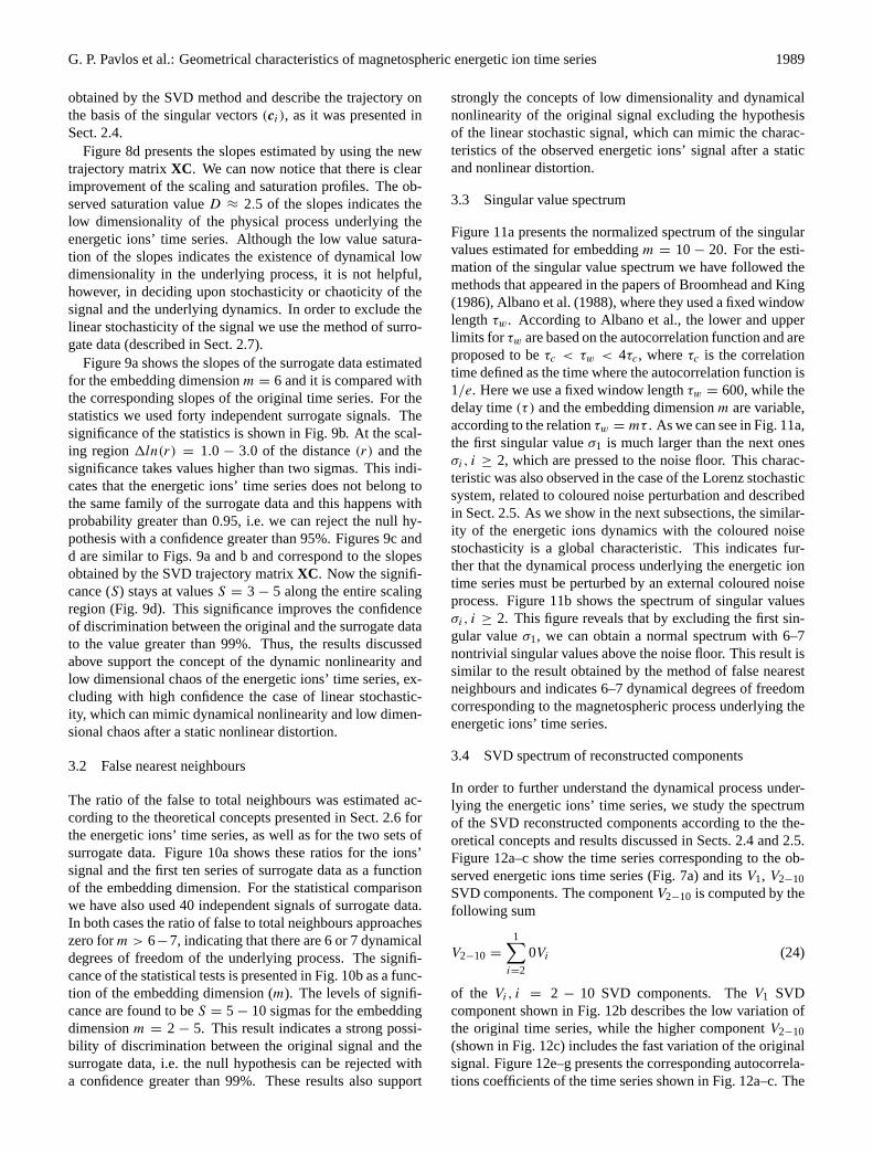
Figure 13 Fig. 13. (a)The slopes of the correlation integrals estimated for theV1 SVD reconstructed component of the energetic ions time series form = 4 − 8, τ = 70 and Theiler’s parameterw = 100. (b) The same as (a) but for the SVD reconstructed componentV2−10 =

∑Vi , (i =

2− 10) with parametersm = 4− 9, t = 7, w = 500. (c) The same as (a) but for theV1 SVD reconstructed component and its surrogate datawith parametersm = 6, t = 70, w = 100. (d) The same as (b) but for theV2−10 SVD reconstructed component and its surrogate data withparametersm = 6, τ = 70, w = 50.

0 5 10 15 20 25i

0.00

0.20

0.40

0.60

0.80

1.00

1.20

tw = 600

m = 20, τ = 30

m = 15, τ = 40

m = 10 , τ = 60

Energetic Ions_V1 (a)

0 5 10 15 20 25i

0.00

0.20

0.40

0.60

0.80

1.00

1.20

tw = 40

m = 20, τ = 2

m = 14, τ = 3

m = 10 , τ = 4

Energetic Ions_(V2-10) (b)

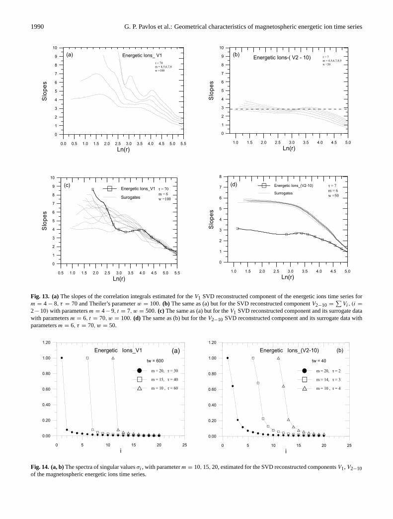
Figure 14 Fig. 14. (a, b)The spectra of singular valuesσi , with parameterm = 10, 15, 20, estimated for the SVD reconstructed componentsV1, V2−10of the magnetospheric energetic ions time series.


autocorrelation coefficient of theV1 component indicates aslow decay profile, while the autocorrelation coefficient oftheV2−10 SVD component shows a fast decay profile. Thesecharacteristics could be explained by a linear stochastic pro-cess related to theV1 component and a nonlinear chaoticprocess underlying theV2−10 SVD component in accordancewith the results discussed in Sect. 2.5.

The above hypothesis is also supported by the resultsshown in Fig. 13. Figure 13a presents the slopes of thecorrelation integrals estimated for theV1 SVD reconstructedcomponent of the energetic ions’ time series. This figure re-veals that theV1 component does not include any low dimen-sional characteristic, as there is no satisfactory scaling andlow value saturation profile of the slopes. Figure 13c presentsthe slopes of the correlation integrals estimated for the surro-gate data of theV1 component for the embedding dimensionm = 6. This figure shows that there is no significant differ-ence between the original signalV1 and the surrogate data.As the surrogate data are produced by a nonlinear distortionof a linear noise, we can conclude the linear character of theV1 signal, while the high dimensionality of theV1 compo-nent was concluded from Fig. 13a. Based on these resultswe can support the concept that theV1 SVD component ofthe ions’ time series is basically the manifestation of an ex-ternal high dimensional coloured noise. This concept is alsosupported strongly by the similarity which can be observedbetween the slopes of the ions’V1 SVD component and theV1 SVD component of the Lorenz system perturbed by anexternal additive coloured noise (see Sect. 2.5).

On the contrary, theV2−10 SVD component of the ionsclearly reveals low dimensionality and nonlinear characteris-tics. Figure 13b and d, are similar to Fig. 13a and c includingthe slopes of theV2−10 component and its surrogate data.The scaling and low dimensional profile of the slopes of theV2−10 component are clearly indicated by Fig. 13b. The non-linearly of theV2−10 signal is supported by Fig. 13d, as itssurrogate data are clearly discriminated by the original sig-nalV2−10. The behaviour of the ions’V2−10 SVD componentcorresponds to the behavior of theV2−10 component of thecoloured noise stochastic Lorenz system (see Fig. 2h). Thisfurther strengthens the supposition about the existence of anexternal high dimensional coloured noise component in themagnetospheric dynamical process underlying the energeticions’ system.

As we have shown in Sect. 2.5, the singular value spec-trum of theV2−10 component of the Lorenz coloured noisestochastic system is similar to the singular value spectrum ofthe original purely deterministic Lorenz system. In oppositecontrast, the singular value spectrum of theV1 componentof the Lorenz coloured noise stochastic system is similar tothe spectrum of the original Lorenz stochastic system, i.e. theV1 component absorbs the main part of the external colourednoise perturbation, while the SVD componentV2−10 remainsalmost unperturbed by the external coloured noise compo-nent, conserving invariant the characteristics of the original(unperturbed) purely deterministic system. The above char-acteristics of coloured noise stochasticity related to low di-

mensional chaos can be used for understanding the singularspectra of theV1, V2−10 SVD components of the energeticions signal, shown in Fig. 14a–b. Figure 14a presents thesingular value spectrum of theV1 component of the ions’time series and Fig. 14b presents the same spectrum for theV2−10 SVD component of the ions signal. The singular spec-trum of theV1 SVD component of the ions’ signal is similarto the singular spectrum of the original time series shownin Fig. 11a, i.e. there is strong asymmetry between the firstand the other singular valuesσi, i ≥ 2 which are pressed tothe noise floor. Contrary to this, the spectrum of theV2−10component is normal, revealing 4–6 nontrivial singular val-ues above the noise background. This analysis can be usedto support the central concept described previously, i.e. theV1 SVD component of the ions’ time series includes mainlythe external coloured noise component, while theV2−10 SVDcomponent includes the internal dynamics of the underlyingmagnetospheric process.

4 Summary and discussion

In this work we have estimated the correlation dimension,the false neighbours and the singular value spectrum for themagnetospheric energetic ions measured at the distant mag-netotail. In addition, the null hypothesis is tested in order toexclude the case where the original time series arises froma linear stochastic process, but the observed time series maybe a nonlinear distortion of the underlying linear time series(Theiler et al., 1992a, b). For the application of the test ofthe null hypothesis we have used surrogate data constructedaccording to Schreiber’s algorithm, to mimic the amplitudedistribution and the power spectrum of the magnetosphericsignal. The significance of the discriminating statistics wasfound to be higher than two sigmas, permitting us to rejectthe null hypothesis with a confidence greater than 95%.

The correlation dimension was found to be∼3 − 4, whilethe false neighbours and the singular value spectrum haveshown∼6 − 7 independent dynamical degrees of freedom.This result is in accordance with the value of the correlationdimension (D2), as the correlation dimension and the maxi-mum number(n) of the degrees of freedom are connected bythe relationn ≤ 2D2 + 1.

Moreover, the SVD analysis has revealed two differentphysical processes related to the magnetospheric dynamicsconcluded by the observed energetic ions’ signal. The firstprocess corresponds to a stochastic external component, aswas indicated by the first SVD component. In this case thetest of the null hypothesis has shown that there is no sig-nificant difference between the surrogate data and the firstSVD component. The second process corresponds to a lowdimensional chaotic component, as was indicated by the re-constructed time series obtained by adding the next SVDcomponents. In this case the test of the null hypothesis hasshown a strong difference in the discrimination of the sur-rogate data and the reconstructed time series. In addition,the Lorenz system perturbed by external coloured noise has


shown a strong similarity with the the ion time series accord-ing to the above chaotic analysis. In particular, the behaviourof the SVD components of the stochastic Lorenz signal andthe magnetospheric ions signal were found to be quite simi-lar for the first component and the reconstructed signal. Thecomparison of Lorenz’s results to those of the ions’ signalsupports the above concept of two independent underlyingphysical processes underlying the observed ions signal. Thefirst process may be related to the stochastic dynamics of thesolar wind system and the second one to the internal low-dimensional chaotic dynamics of the magnetospheric system.Finally, the above results are in complete agreement with theprevious results obtained by the chaotic analysis of magne-tosphericAE index.

Acknowledgements.Topical Editor T. Pulkkinen thanks two refer-ees for their help in evaluating this paper.

References

Abarbanel, H. D., Brown, R., Sidorowich, J. J., and Tsirming, L. S.:The analysis of observed chaotic data in physical systems, Rev.Mod. Phys. 65, 1331–1392, 1993.

Albano, A. M., Muench, J., Schwarzt, C., Mees, A. I., and Rapp,P. E.: Singular value decomposition and the Grassberger Pro-caccia algorithm, Physical Review A, 38(6), 3017–3026, 1988.

Anagnostopoulos, G. C., Sarris, E. T., and Krimigis, S. M.: Magne-tospheric origin of energetic (E ≥ 50 keV) ions upstream of thebow shock: The October 31, 1977 event, J. Geophys. Res. 91,3020–3028, 1986.

Anagnostopoulos, G. C., Rigas, A. G., Sarris, E. T., and Krim-igis, S. M.: Characteristics of upstream energetic (E ≥ 50 keV)ion events during intense geomagnetic activity, J. Geophys. Res.,103, 9521–9533, 1998.

Argyris, J., Andreadis, I., Pavlos, G., and Athanasiou, M.: The in-fluence of noise on the correlation dimension of chaotic attrac-tors, Chaos, Solitons, and Fractals, 9, 343–361, 1998a.

Argyris, J., Andreadis, I., Pavlos, G., and Athanasiou, M.: On theinfluence of noise on the Largest Lyapunov exponent and on thegeometric structure of attractors, Chaos, Solitons & Fractals, 9,947–958, 1998b.

Athanasiu, M. A. and Pavlos, G. P.: SVD analysis of the Mag-netosphericAE index time series and comparison with low di-mensional chaotic dynamics, Nonlin. Proc. Geophys., 8, 95–125,2001.

Baker, D. N., Klimas, A. J., McPherron, R. L., and Bucher, J.: Theevolution from weak to strong geomagnetic activity: an interpre-tation in terms of deterministic chaos, Geophys. Res. Lett., 17,41–44, 1990.

Brogan, W. L.: Modern control theory, Prentice Hall, EnglewoodCliffs, New Jersey, 1982.

Broomhead, D. S. and King, G. P.: Extracting qualitive dynamicsfrom experimental data, Physica D, 20, 217–236, 1986.

Broomhead, D. S., Huke, J. P., and Muldoon, M. R.: Linear filtersand nonlinear systems, J.R. Statist. Soc. B, 1992.

Casdagli, M., Jardin, D. D., Eubank, S., Farmer, J. D., Gibson, J.,Hunter, N., and Theiler, J.: Non linear modeling of chaotic timeseries: Theory and applications, Los Alamos National Labora-tory Preprint LA-UR91–1637, 1991.

Christon, S. P., Desai, M. I., Eastman, T. E., Gloeckler, G.,Kokubun, S., Lui, A. T. Y., McEntire, R. W., Roelof, E. C., andWilliams, D. J.: Low-chargestate heavy ions upstream of Earth’sbow shock and sunward flux of ionospheric O+1, N+1, and O+2

Ions: Geotail Observations, Geophys. Res. Lett., 27, 2433–2436,2000.

Ding, M., Grebogi, C., Ott, E., Sauer, T., and York, J. A.: Estimatingcorrelation dimension from a chaotic time series: when does aplateau onset occur?, Physica D 69, 404–424, 1993.

Eastman, T. E. and Christon, S.: Ion composition and transportnear the Earth’s magnetopause, in: Geophysical monograph 90,Physics of the Magnetopause, edited by Song, P., Sonnerup,B. U. O., and Thomsen, M. F., 131–137, 1995.

Elsner, J. B. and Tsonis, A. A.: Singular spectrum analysis, a newtool in time series analysis, Plenum Press, New York, 1996.

Farmer, D. J. and Sidorowich, J. J.: Predicting chaotic time series,Phys. Rev. Lett. 59, 845–848, 1987.

Freeman, T. J. and Parks, G. K.: Fermi acceleration of suprathermalsolar wind ions, J. Geophys. Res., 105, 15 715–15 727, 2000.

Goode, B., Cary, J. R., Doxas, I., and Horton, W.: Differentiatingbetween colored random noise and deterministic chaos, J. Geo-phys. Res., 106, 21, 277, 2001.

Grassberger, P. and Procaccia, I.: Measuring the strangeness ofstrange attractors, Physica. D, 9, 189–208, 1983.

Ipavich, F. M., Scholer, M., and Gloeckler, G.: Temporal develop-ment of composition, spectra, and anisotropies during upstreamparyticle events, J. Geophys. Res., 86, 11 153–11 160, 1981.

Kirsch, E., Pavlos, G. P., and Sarris, E. T.: Evidence for particleacceleration processes in the magnetotail, J. Geophys. Res., 89,1003–1007, 1984.

Klimas, A. J., Baker, D. N., Roberts, D. A., Fairfield, D. H., andBuchner, J. A.: A Nonlinear dynamic model of substorms, Geo-phys. Monog. Ser., vol. 64, edited by Kan, J. R., Potemra, T. A.,Kokumun, S. and Iijima, T., 449–59, AGU, Washington, D.C.,1991.

Klimas, A. J., Baker, D. N., Roberts, D. A., and Fairfield, D. H.: Anonlinear dynamical analogue model of geomagnetic activity, J.Geophys. Res., 97, 12 253–12 266, 1992.

Klimas, A. J., Vassiliadis, D., Baker, D. N., and Roberts, D. A.: Theorganized nonlinear dynamics of the magnetosphere, J. Geophys.Res., 101, 13 089–13 113, 1996.

Kugiumtzis D.: State space reconstruction parameters in the anal-ysis of chaotic time series-the role of the time window length,Physica D, Vol. 95, 13–28, 1996.

Osborne, A. R. and Provenzale, A.: Finite correlation dimensionfor stochastic systems with power-low spectra, Physica D, 35,357–381, 1989.

Pavlos, G. P., Sarris E. T., and Kallabetsos, G.: Monitoring of en-ergy spectra of particle bursts in the plasma sheet and magne-tosheath, Planet. Space Sci., 33, 1109–1118, 1985.

Pavlos, G. P.: Magnetospheric dynamics, in: Proc. Symposium onSolar and Space Physics, edited by Dialetis, D., National Obser-vatory of Athens, Athens, 1-43, 1988.

Pavlos, G. P., Rigas, A. G., Dialetis, D., Sarris, E. T., Karakatsanis,L. P., and Tsonis, A. A.: Evidence for chaotic dynamics in outersolar plasma and the earth magnetopause, in: Chaotic Dynamics:Theory and Practice, edited by Bountis, A., Plenum, New York,327–339, 1992a.

Pavlos, G. P., Kyriakou, G. A., Rigas, A. G., Liatsis, P. I., Tro-choutos, P. C., and Tsonis, A. A.: Evidence for strange attrac-tor structures in space plasmas, Ann. Geophysicae, 10, 309–322,1992b.


Pavlos, G. P., Diamadidis, D., Adamopoulos, A., Rigas, A. G.,Daglis, I. A., and Sarris, E. T.: Chaos and magnetospheric dy-namics, Nonlin. Proc. Geophys., 1, 124–135, 1994.

Pavlos, G. P., Athanasiu, M., Kugiumtzis, D., Hantzigeorgiu, N.,Rigas A. G., and Sarris, E. T.: Nonlinear analysis of Magneto-spheric data, Part I. Geometric characteristics of theAE indextime series and comparison with nonlinear surrogate data, Non-lin. Proc. Geophys., 6, 51–65, 1999a.

Pavlos, G. P., Kugiumtzis, D., Athanasiu, M., Hantzigeorgiu, N.,Diamantidis, D., and Sarris, E. T.: Nonlinear analysis of Mag-netospheric data, Part II, Dynamical characteristics of theAE

index time series and comparison with nonlinear surrogate data,Nonlin. Proc. Geophys., 6, 79–98, 1999b.

Pavlos, G. P., Athanasiu, M., Diamantidis, D., Rigas, A. G., andSarris, E.: Comments and new results about the magnetosphericchaos hypothesis, Nonlin. Proc. Geophys., 6, 99–127, 1999c.

Price, C. P. and Prichard, D.: The non-linear responce of the mag-netosphere: 30 October 1978, Geophys. Res. Lett., 20, 771–774,1993.

Price, C. P., Prichard, D., and Bischoff, J. E.: Nonlinear input/outputanalysis of the auroral electrojet index, J. Geophys. Res., 99,13 227–13 238, 1994.

Prichard, D. J. and Price, C. P.: Spurious dimensions estimatesfrom time series of geomegnetic indices, Geophys. Res. Lett.,19, 1623–1626, 1992.

Prichard, D. J. and Price, C. P.: Is theAE Index re result of nonlin-ear dynamics? Geophys. Res. Lett., 20, 2817–2820, 1993.

Prichard, D. J.: Short comment for magnmetospheric chaos, Non-linear Proc. Geophys., 20 771-20 774, 1995.

Priestley, M. B.: Nonlinear and non-stationary time series analysis,Academic Press, 1988.

Provenzale, A., Osborne, A. R., Kirwan, Jr., A. D., and Berga-masco, L.: The study of fluid parcel trajectories in large-scaleocean flows, in: Nonlinear Topics in Ocean Physics, edited byOsborne, A. R., Elsevier, Paris, 367–402, 1991.

Provenzale, A., Smith, L. A., Vio, R., and Murante, G.: Distinguish-ing low dimensional dynamics and randomness in measured timeseries, Physica D, 58, 31–49, 1992.

Roberts, D. A., Baker, D. N., Klimas A. J., and Bargatze, L. F.:Indications of low dimensionality in magnetospheric dynamics,Geophys. Res. Lett., 18, 151–154, 1991.

Sarafopoulos, D. V., Atahanasiu, M. A., Sarris, E. T., Yamamoto,T., and Kokubun, S.: Properties and origin of energetic particlesat the duskside of the Earth’s magnetosheath throughout a greatstorm, Ann. Geophysicae, 17, 1121–1133, 1999.

Sarafopoulos, D. V., Atahanasiu, M. A., Sibeck, D. G., McEntire,R. W., Sarris, E. T., and Kokubun, S.: Energetic protons andelectrons dispersion signatures in the nightside magnetosheathsupporting their leakage out of the magnetopause, J. Geophys.Res., 105, 15 729–15 739, 2000.

Schreiber, T. and Schmitz, A.: Improved surrogate data for nonlin-

earity test, Phys. Rev. Lett., 77, 635–638, 1996.Schreiber T.: Constrained randomization of time series data, Phys.

Rev. Lett., 80, 2105–2108, 1998.Shan, H., Hansen, P., Goertz, C. K., and Smith, K. A.: Chaotic

appearance of theAE Index, Geophys. Res. Lett., 18, 147–150,1991.

Takens, F.: Detecting strange attractors in turbulence, in: Vol. 898of Lectures Notes in Mathematics, edited by Rand, D. A. andYoung, L. S., 366–381, Springer, Berlin, 1981.

Takens, F.: On the numerical determination of the dimension ofan attractor, in dynamical systems and bifurcations, Groningen1984, in: vol. 1125 of Lecture Notes in Mathematics, editedby Braakama, B. L. J., Broer, H. W., and Takens, F., Berlin,Springer-Verlag, 99–106, 1985.

Theiler, J.: Some comments on the correlations dimensions of 1/f

a noise, Phys. Lett. A, 155, 480–493, 1991.Theiler, J., Galdikian, B., Longtin, A., Eubank, S., and Farmer,

J. D.: Using surrogate data to detect nonlinearity in time series,in: Nonlinear Modeling and Forecasting, vol. XII of SFI stud-ies in the Sciences of Complexity, edited by Casdagli, M. andEubank, S., Addison-Wesley, Reading, Mass., 163–188, 1992a.

Theiler, J., Eubank, S., Longtin, A., Galdikian, B., and Farmer,J. D.: Testing for nonlinearity in time series: the method of sur-rogate data, Physica D, 58, 77–94, 1992b.

Theiler, J., Lisay, P. S., and Rubin, D. M.: Detecting nonlinearity indata with long coherence times, Times series prediction: Fore-casting the future and understanding the past, in: SFI studies inthe Sciences of Complexity, Proc. Vol. XV, edited by Weigend,A. S. and Gershenfeld, N. A., Addison-Wesley, 429–455, 1993.

Tong, H.: Non-linear time series, a dynamical system approach,Oxford University Press, New York, 1990.

Tsonis, A. A.: Chaos: from theory to applications, Plenum, NewYork, 1992.

Vassiliadis, D., Sharma, A. S., Eastman, T. E., and Papadopoulos,K.: Low-Dimensional chaos in magnetospheric activity fromAE

time series, Geophys. Res. Lett., 17, 1841–1844, 1990.Vassiliadis, D., Sharma, A. S., and Papadopoulos, K.: Time series

analysis of magnetospheric activity using nonlinear dynamicalmethods, in: Chaotic Dynamics: Theory and Practice, edited byBountis, T., Plenum, New York, 1992.

Voros, Z.: Synergetic approach to substorm phenomenon, in: Mag-netospheric substorms, Geoph. Monog. Ser. Vol. 64, edited byKan, J. R., Potemra, T. A., Kokubun, S., and Iijima, T., AGU,Washington, D.C., 461–467, 1991.

Weigend, A. S. and Gershenfeld, N. A.: Time Series Prediction:Forecasting the Future and Understanding the Past, Addison-Wesley Publishing Company, Reading, 1994.

Williams, D. J., McEntire, R. W., Schemm II, C., Lui, A. T. Y.,Gloeckler, G., Christon, S. P., and Gliem, F.: GEOTAIL en-ergetic particles and ion composition instrument, J. Geomagn.Geoelectr., 46, 39–57, 1994.

Geometrical characteristics of magnetospheric energetic ion time series: evidence for low...

Documents

Transcript of Geometrical characteristics of magnetospheric energetic ion time series: evidence for low...