Cold magnetospheric plasma flows: Properties and interaction ...

Cold magnetospheric plasma flows:

Properties and interaction with spacecraft

Licentiate Thesis

by

Erik Engwall

Department of Astronomy and Space Physics

Uppsala University

SE-75120 Uppsala, Sweden

March 10, 2006

Abstract

The ionosphere constantly loses matter to the surrounding magnetosphere throughdifferent outflow processes, and it is probably the main source of plasma supply to themagnetosphere. The ionospheric plasma has low energy and when flowing out fromthe Earth along diverging magnetic field lines, the density decreases. This will makethe plasma ions difficult to detect with spacecraft, since the low density ensures a highspacecraft potential, which the low-energy ions will not be able to overcome. Therefore,only few observations of tenuous, cold plasma have been made, in spite of its abundancein the magnetosphere.

In this thesis, we present a new method for detecting and studying cold plasma withthe double-probe electric field instrument EFW on the Cluster spacecraft. In coldflowing plasmas EFW observes a negatively charged spacecraft wake, which can beused to derive the flow speed of the cold plasma. The method has been verified fora case in the magnetotail at 18 RE from the Earth, where a very special and unusualsetup of the four Cluster spacecraft allowed simultaneous measurements of the ions withparticle detectors. We have then applied the method for an initial statistical study ofthree months of Cluster data in the magnetotail lobes. The resulting flow parametersshow agreement with previous measurements of ion outflow at lower altitudes, andthe method opens up for observing cold flowing ions in regions where they previouslyhave been inaccessible to spacecraft. To better understand the observed wake fields inEFW data, we have studied properties of enhanced wakes by numerical simulations,theoretical reasoning and data analysis. As an introduction to these new results, wehave reviewed important measurements of cold magnetospheric plasmas, functioning ofdouble-probe measurements, and spacecraft-plasma interactions, such as wake effects.

Erik EngwallDepartment of Astronomyand Space Physics,Uppsala UniversityBox 515SE-751 20 [email protected]

List of Papers

This thesis is based on the following papers:

Paper I

E. Engwall, A. I. Eriksson, J. Forest, Wake formation behind positively chargedspacecraft in flowing tenuous plasmas, Phys. Plasmas, in review, 2006.

Paper II

E. Engwall, A. I. Eriksson, Double-probe measurements in cold tenuous space plasmaflows, IEEE Trans. Plasma Sci., in review, 2006.

Paper III

E. Engwall, A. I. Eriksson, M. Andre, I. Dandouras, G. Paschmann, J. Quinn, andK. Torkar, Low-energy (order 10 eV) ion flow in the magnetotail lobes inferred fromspacecraft wake observations, Geophys. Res. Lett., accepted, 2006.

Contents

1 Introduction 1

2 Space plasma 3

2.1 The space environment . . . . . . . . . . . . . . . . . . . . . . . . . . . . 3

2.2 Properties of a plasma . . . . . . . . . . . . . . . . . . . . . . . . . . . . 5

2.3 Cold plasma in the magnetosphere . . . . . . . . . . . . . . . . . . . . . 6

3 Probe measurements of plasma 15

3.1 Probe currents in Maxwellian plasmas . . . . . . . . . . . . . . . . . . . 15

3.2 Probe measurements of densities and temperatures . . . . . . . . . . . . 22

3.3 Electric field measurements with double probes . . . . . . . . . . . . . . 23

4 Spacecraft-Plasma Interactions 28

4.1 Spacecraft charging . . . . . . . . . . . . . . . . . . . . . . . . . . . . . . 28

4.2 Wake effects . . . . . . . . . . . . . . . . . . . . . . . . . . . . . . . . . . 29

5 Wake effects in Cluster electric field data 32

5.1 The Cluster satellites . . . . . . . . . . . . . . . . . . . . . . . . . . . . . 32

5.2 Electric field measurements from Cluster . . . . . . . . . . . . . . . . . . 33

5.3 Influence of wake on Cluster EFW . . . . . . . . . . . . . . . . . . . . . 34

6 Studying cold plasma flows with electric field instruments 37

6.1 A new method for measuring plasma flows . . . . . . . . . . . . . . . . . 37

6.2 Initial statistical study of cold plasma flows . . . . . . . . . . . . . . . . 38

7 Summary of publications 42

7.1 Paper I: Wake formation behind positively charged spacecraft in flowingtenuous plasmas . . . . . . . . . . . . . . . . . . . . . . . . . . . . . . . 42

7.2 Paper II: Double-probe measurements in cold tenuous space plasma flows 43

7.3 Paper III: Low-energy (order 10 eV) ion flow in the magnetotail lobesinferred from spacecraft wake observations . . . . . . . . . . . . . . . . . 43

v

Chapter 1

Introduction

The light from the aurora has challenged the imagination of people of all times. Thismainly green light emitted by excited atoms and molecules in the Earth’s atmospherecan be seen as the messenger of phenomena occurring due to the interaction betweenthe Sun and Earth. From the Sun a large amount of plasma, i.e. ionised gas, with highenergy is constantly expelled out into the solar system. This is the solar wind. TheEarth is protected from the solar wind mainly by its magnetic field, creating a shieldaround the Earth, called the magnetosphere. The solar wind and the magnetosphereare both highly dynamic regions, where a vast number of different processes occur,some of which creates the aurora.

The current knowledge of the processes in the magnetosphere, the solar wind and theareas in between, can to a large extent be attributed to the large number of scientificsatellites, launched during the past 30 years1. All new experimental results presentedin this thesis are based on measurements from the Cluster II mission, which is oneof today’s most ambitious projects, with four satellites flying in formation to exploresome of the key regions in the near-Earth space. In our work, we have mainly usedmeasurements from the two Cluster electric field instruments, and especially from theElectric Fields and Waves instrument (EFW) (Gustafsson et al., 2001), which measurespotential differences between two spherical probes.

A scientific spacecraft will always more or less affect the plasma environment it issent out to investigate, since spacecraft interact with the surrounding plasma. Oneimportant example of spacecraft-plasma interaction is that spacecraft can charge tohigh negative potentials, which disturbs the electric fields in the plasma. Moreover, thespacecraft charging can be hazardous for the spacecraft itself, since uneven chargingbetween different electrical elements of the spacecraft might lead to discharges possiblydestroying critical systems on the spacecraft. Most magnetospheric spacecraft, likeCluster, will not experience such problems, as they are constructed with conductivesurfaces and charge to positive potentials of the order of a few tens of volts because ofphotoelectron emission. However, this positive spacecraft potential makes it difficult tomeasure low-energy ions with energy less than the equivalent energy of the spacecraftpotential, since these ions will not be able to climb the potential barrier. This is the casefor cold, tenuous magnetospheric plasmas.2 The ionosphere, which is the upper part

1Ground based measurements have also been of great importance for the exploration of the near-Earth space.

2In this thesis, we define cold as temperatures on the order of a few eV and tenuous as densities on

1

2 CHAPTER 1. INTRODUCTION

of Earth’s atmosphere, is supposed to be the main source of magnetospheric plasmaand the cold plasma in the magnetosphere is certainly of ionospheric origin Chappellet al. (1987); Chappell et al. (2000). To understand the plasma transport, as well asheating mechanisms in the magnetosphere, it is therefore important to study these coldplasmas. However, due to the positive potential on sunlit magnetospheric spacecraftfew reliable observations of cold magnetospheric plasmas have been made.

Another spacecraft-plasma interaction problem is negatively charged wakes formingbehind spacecraft in motion with respect to the plasma. These wakes may under cer-tain circumstances grow big for positive spacecraft potentials and create large spuriouselectric fields, which has been observed in Cluster EFW data (Eriksson et al., 2006a).Even though, in the beginning only seen as a contamination to the real electric fieldmeasurements, the wake spurious electric field can be used to detect and derive theflow velocity cold magnetospheric plasmas. Information on the functioning of probesand double-probe instruments, as well as how the wakes form is essential to understandthese methods.

This thesis consists of two parts: a few introductory chapters accompanied by threescientific papers. Chapter 2 gives first an introduction to our space environment andsome basic properties of a plasma. The rest of the chapter contains a more extensivetreatment of observations and mechanisms for supply of cold magnetospheric plasmas.The starting point in chapter 3 is basic probe theory containing a detailed treatment ofthe currents to a probe in a plasma. Further, we examine the use of probes in differentplasma instruments, focusing mostly on the operations and possible complications ofdouble-probe instruments for measurements of electric fields. Chapter 4 treats twoimportant phenomena of spacecraft-plasma interactions: spacecraft charging and wakeeffects. In chapter 5 we move on to the wake effects experienced by the EFW instrumenton Cluster, starting with some general information on the Cluster spacecraft and theirelectric field instruments. In chapter 6, we present our new method for deriving theflow velocity of cold ions with electric field instruments, and show results for an initialstatistical study of cold ions using this method. Finally, chapter 7 summarizes thethree papers. The first paper (Engwall et al., 2006b) treats the formation of enhancedwakes behind spacecraft, including numerical simulations and theoretical reasoning.The second paper (Engwall and Eriksson, 2006) includes detailed data analysis of thewake field detected by EFW. In the third paper (Engwall et al., 2006a) we report coldions in the magnetotail detected by two methods: (1) direct measurements with an iondetector, and (2) measurement of the wake electric field by EFW.

the order of tenths of cm−3.

Chapter 2

Space plasma

2.1 The space environment

Space and phenomena in the sky have fascinated mankind for millennia. With theinvention of the telescope and its further development, discoveries revealing some ofthe mysteries of our solar system, galaxy and the whole universe have been made.Nevertheless, it was not until the satellite era, which started with the launch of theSoviet satellite Sputnik 1 in 1957, that it was possible to explore the near-Earth spaceenvironment in detail. An adequate description of this environment is necessary tounderstand such a common and relatively close phenomenon as the aurora borealis.This section is intended to give a brief introduction to the space environment aroundus. For a more detailed description, books on space physics, for example Kivelson andRussel (1995), Parks (1991) and Gombosi (1998), are recommended.

The existence of the Sun is necessary, either directly or indirectly, for all life on Earth.As everybody knows, energy is transported from the Sun in form of electromagneticradiation, which among others will give us enough heat and light and allow plants togrow. What is less known, is that as much as 1% of the energy from the Sun reachingthe Earth is in form of charged particles (Sandahl , 1998). The Sun does, in fact, notonly emit light, but also a high-speed stream of particles, at a rate of 1 million tons/s.This stream of plasma is called the solar wind. The solar wind plasma originates in theouter layers of the Sun, thus consisting mostly of protons, electrons and a small amountof helium ions. Some of these particles will eventually reach the Earth, but this is onlya tiny fraction of all the particles in the solar wind, since the Earth is shielded by itsmagnetic field. This magnetic shield protects us from the highly energetic solar windplasma, which has an average speed of 450 km/s and temperature of 100 000 K.

The solar wind is deflected around the Earth’s magnetic field, compressing it in thesunward direction and extending it in the anti-sunward direction (see figure 2.1). Sincethe solar wind is supersonic at the orbit of the Earth, a shock wave will form around theEarth reducing the speed of the solar wind plasma to subsonic values. This happensat the bow shock. Shocked solar wind particles continue into the magnetosheath, wherethey are re-accelerated to supersonic flow velocities. The magnetopause is the borderto the Earth’s magnetosphere, which is the region dominated by the Earth’s magneticfield. The solar wind experiences difficulties to enter the magnetosphere through themagnetopause. However, in the cusp regions the magnetic field lines of the solar wind

3

4 CHAPTER 2. SPACE PLASMA

are connected to the Earth’s magnetic field, which will allow solar wind plasma topenetrate the magnetosphere. The magnetotail is a cold tenuous region in the magne-tosphere, extending from the dusk side of the Earth far out into the solar wind. Also inthe plasma sheet the plasma density is low, but here the particle energies are high, mak-ing the plasma hot. The plasmasphere is the torus-shaped region closest to the Earthwith a cold dense plasma. Above the geomagnetic poles, the polar caps are found.They are bounded by the auroral regions, where the aurora1 appears, when chargedparticles (mostly electrons) from the magnetosphere enter the atmosphere of the Earthand collide with atoms and molecules, typically at an altitude of 100 km. In the colli-sions, the atmospheric atoms and molecules will be excited, and when de-excited, lightwill be emitted. This light can be seen in the sky at clear nights.

Current theories suggest that most of the plasma in the magnetosphere originates fromthe ionosphere (Chappell et al., 1987; Chappell et al., 2000). If the ionospheric plasmais sufficiently energised, it can escape into the magnetosphere by several different pro-cesses. An example of such a process is the polar wind, which is an up-flowing stream ofionospheric plasma along the open geomagnetic field lines in the polar cap. In section2.3, we examine the different mechanisms of supply of ionospheric plasma, which iscold, to the magnetosphere.

Figure 2.1: Schematic view of the magnetosphere. The numbers correspond to seven different observa-tions of cold magnetospheric plasma presented in section 2.3.2. (Dashed ellipses represent observationsin the southern hemisphere.) 1. High altitude polar wind studied by Su et al. (1998), Moore et al. (1997)and Chappell et al. (2000). 2-4. Cold plasma in the magnetotail observed by Etcheto and Saint-Marc

(1985), Seki et al. (2003) and Sauvaud et al. (2004). 5. Cold ions in the magnetotail lobes studiedby Engwall et al. (2006a). 6-7. Studies of cold plasma populations in the dayside magnetosphere byChen and Moore (2004) and Sauvaud et al. (2001). (Original figure adapted from Kivelson and Russel

(1995).)

1The aurora is often referred to as the northern lights or polar lights.

2.2. PROPERTIES OF A PLASMA 5

2.2 Properties of a plasma

Plasma is the dominating state of matter in the universe, estimated to comprise around99% of all observable matter. The lower part of the Earth’s atmosphere is one ofthe few exceptions, where plasma does not play an important role. Because of thisabundance of plasma in the universe, we will need knowledge in plasma physics tounderstand phenomena in space. Even a short comprehensive summary of the theoryof plasma physics is beyond the scope of this thesis2. However, we need to know somebasic principles for the study of cold magnetospheric plasmas and its interaction withspacecraft.

One important feature of a plasma is that it will exhibit collective behaviour, whichmeans that the plasma particles will be governed by the long-range electromagneticforces instead of collisions like in a normal gas. The phenomenon of Debye shieldingis a fundamental property of a plasma and gives an example of collective behaviour.When a charged object is immersed in a plasma, the potential around it will be shieldedout by either the ions or the electrons. A positively charged object will namely attract acloud of electrons, while a negatively charged object will be enclosed in an ion cloud. Ifthe plasma is cold, the shielding will be perfect outside the cloud. For warmer plasmas,however, the small potentials at the edge of the clouds, will not be able to preventthe electrons or ions from escaping. To get a notion of the size of the shielding cloud,we introduce the Debye length, which is a characteristic length for the shielding of thepotential around a charged object. The Debye length, λD, is defined by the expression

λD =

√

ε0KTe

nq2e

, (2.1)

where ε0 is the constant of permittivity, K the Boltzmann constant, Te the electrontemperature, n the plasma density3 at infinity and qe the electron charge. It is worth-while to note that the Debye length will increase when the temperature increases, whichcan be explained by the fact that the augmentation of the thermal motion of the plasmaparticles will make the shielding weaker. Conversely, a dense plasma will make the De-bye length shorter, as there are more particles to shield out the potential. A criterionfor a plasma is that it is quasineutral. This is fulfilled when the dimensions of thephysical system are much larger than the Debye length, since every local concentrationof charge will be shielded in a distance much smaller than the size of the system.

Considering only the individual plasma particles, we can find some useful relations fortheir motion in electromagnetic fields, here taken to be constant both in time and space.The equation of motion for a particle with mass mα, charge qα and velocity vα underthe influence of an electric field E, and a magnetic field B is given by

mαdvα

dt= qα(E + vα × B) (2.2)

If the electric field is zero (E = 0) and vα is perpendicular to B, equation 2.2 onlydescribes a circular motion with the Lorentz force as the central force (Fc = qαvα×B).

2Chen (1984) gives a good introduction to plasma physics and is used as the main reference for thissection.

3The plasma density is expressed in particles per unit volume.


The angular frequency of this motion is the cyclotron angular frequency, ωc = |qαB|mα

,

and the radius is the Larmor radius, rL =vα,⊥

ωc. If the velocity has a component along

the magnetic field, the particle will move in a spiral. The projection of the motion ontothe plane perpendicular to B will, however, still be a circle with the same centre asbefore. For non-zero electric fields the particle will drift with a velocity E × B/B 2,thus in a direction perpendicular to both the electric and magnetic fields.

An interesting property of a moving plasma is that, for slow time variations, the mag-netic field lines follow the plasma motion, and they are thus referred to as frozen-infield lines. The volume bounded by a set of field lines is called a flux tube, and thefrozen-in condition implies that particles initially linked to a certain flux tube remainsfixed to it throughout the plasma motion. The frozen-in condition is satisfied if theplasma motion can be approximated by

E + v × B ≈ 0, (2.3)

where v is the velocity of the plasma, which will be equivalent to the single particle driftfor non-zero electric fields, E ×B/B2. For many applications in space physics, such asthe description of plasma convection in the magnetosphere, the frozen-in condition isa very useful approximation.

Because of the electromagnetic properties of plasma, different types of oscillations willarise. The simplest type are the plasma oscillations. The light electrons will, because oftheir inertia, oscillate back and forth against a uniform background of massive immobileions, with a characteristic frequency, the plasma frequency. The plasma frequency, ωpe

is given by

ωpe =

√

n0e2

ε0m(2.4)

The quantity ω−1pe is often chosen as a characteristic time scale for plasmas.

2.3 Cold plasma in the magnetosphere

2.3.1 Mechanisms for supply of cold magnetospheric plasmas

The cold plasma in the magnetosphere is mainly of ionospheric origin. Ionosphericplasma has low energy, and if it is permitted to escape into the magnetosphere withoutsignificant heating, it will remain cold. The total outflow of ions from the ionosphere isestimated to approximately 1 kg/s. These outflows can be divided into two types (Yauand Andre, 1997):

1. Bulk ion outflows

2. Energisation processes where only a fraction of the ions are energised

Ion energisation processes include for example transversely accelerated ions, ion con-ics and ion beams. In these processes only a fraction of the ions participate in the

2.3. COLD PLASMA IN THE MAGNETOSPHERE 7

outflow. This is in contrast to the bulk ion outlows, where the whole particle distribu-tion is moving. These outflows can thus contribute significantly to the population ofcold magnetospheric plasma. The polar wind is an example of bulk ion outflow alongmagnetic field lines above the polar caps. However, bulk ion outflows occur at all lati-tudes; e.g. outflows of thermal O+ in the topside auroral ionosphere, and the filling ofthe plasmasphere are both due to such processes. The bulk ion outflows are stronglydependent on the solar wind properties and the interplanetary magnetic field (Cullyet al., 2003).

Beside bulk ion outflows, the plasmasphere is an important supply of cold plasma to therest of the magnetosphere. The plasmasphere is directly connected to the ionosphereand is thus filled with cold, dense plasma. At plasmasphere detachments, a part of theplasmasphere is ripped away and cold plasma is lost to the magnetosphere.

Polar wind

The polar wind, named after its similarities to the solar wind, was theoretically pre-dicted by Axford (1968) and Banks and Holzer (1968) by arguing that the light ions inthe ionosphere are too energised to be bound by gravity. The outflow is driven by thegradient in the electron pressure, which makes the electrons move upward. To maintaincharge neutrality, an ambipolar electric field is built up and the ions are dragged up-ward along with the electrons. Thus, a larger outflow of electrons automatically givesrise to a larger outflow of ions. This is evident for example in the polar wind on fieldlines connecting to the sunlit ionosphere, where the outflows are significantly largerthan on the nightside, due to escaping photoenergised atmospheric electrons (Yau andAndre, 1997; Moore et al., 1999).

Auroral Bulk outflows

The outflows from the auroral regions are driven by the same processes as the polarwind. However, in these regions the ions are more strongly accelerated, as a result ofparallel electric fields and particle-wave interactions (Moore et al., 1999). Due to theacceleration, heavy ions are also allowed to escape from the ionosphere and the outflowcontains a significant, if not dominant, fraction of O+ (Yau and Andre, 1997; Mooreet al., 1999). The upflowing ions originating in the dayside auroral regions, the cleft,will be transported tailward by antisunward convection. This motion of ions forms thecleft ion fountain (Lockwood et al., 1985).

Plasmasphere detachment

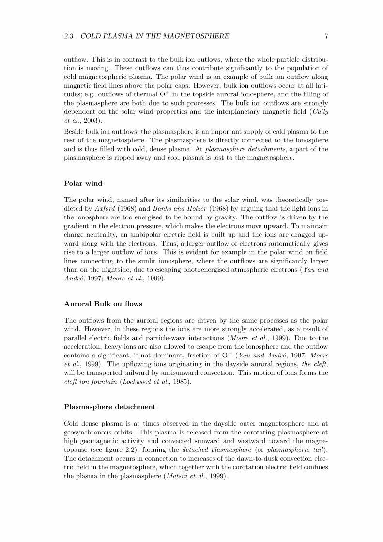
Cold dense plasma is at times observed in the dayside outer magnetosphere and atgeosynchronous orbits. This plasma is released from the corotating plasmasphere athigh geomagnetic activity and convected sunward and westward toward the magne-topause (see figure 2.2), forming the detached plasmasphere (or plasmaspheric tail).The detachment occurs in connection to increases of the dawn-to-dusk convection elec-tric field in the magnetosphere, which together with the corotation electric field confinesthe plasma in the plasmasphere (Matsui et al., 1999).


Figure 2.2: Schematic picture of a plasmaspheric detachment. (Adapted from Matsui et al. (1999).)

2.3.2 Observations of cold flowing plasmas in the magnetosphere

Observations of cold space plasmas with energies on the order of a few eV often en-counter difficulties. The problems occur especially in low-density regions, where thespacecraft potential can reach several tens of volts (see section 4.1). Low-energy ionswill be shielded out by the potential barrier and will never be able to reach any iondetector mounted on the spacecraft. This leads to the conclusion that there may exista much larger fraction of cold plasma in the magnetosphere than has been revealedby previous and current spacecraft missions. In this section, we will investigate someimportant observations, where the geophysical setting or the spacecraft setup has al-lowed detection of cold plasmas in different regions of the magnetosphere. Figure 2.1summarises where these observations have been carried out. References to other in-vestigations of cold ions can be found in the introduction of Paper III (Engwall et al.,2006a).

Polar regions

Measurements of the polar wind have indeed been problematic, due to its tenuouscold plasma. The first direct measurements of the polar wind was achieved in the late1960’s by Explorer 31, which found H+ outflows at 500 and 3000 km with velocitiesup to 15 km/s (Hoffman, 1970). ISIS 2 confirmed the outflow of H+, but also foundevidence for outflows of He+ and O+. Oxygen was shown to be the dominant ionspecies at the satellite altitude (1400 km) during magnetically quiet times (Hoffmanet al., 1974; Hoffman and Dodson, 1980). The measurements from both Explorer 31and ISIS 2 were carried out at low altitude, where the densities were high and thus thespacecraft potentials low. Contributions to the understanding of the polar wind havealso been made by DE 1 (Nagai et al., 1984). The current knowledge of the polar windcan mainly be attributed to studies by Akebono (Abe et al., 1993, 1996) and Polar (Suet al., 1998; Moore et al., 1997; Chappell et al., 2000). The Polar spacecraft was launchedin 1996 into a polar ecliptical orbit with 9 RE apogee (northern hemisphere) and 1.8RE perigee (southern hemisphere). Polar carries the ion detector TIDE (ThermalIon Dynamics Experiment), which operates with good resolution in the 0.3-450 eV


energy range. Together with the Plasma Source Instrument (PSI), which reduces thespacecraft potential to approximately +2 V by creating a plasma cloud around thespacecraft, TIDE is able to measure low-energy ions. These two instruments have shednew light on the dynamism and composition of the polar wind at different altitudes,and also confirmed the existence of the high-altitude polar wind (Moore et al., 1997).

Su et al. (1998) used Polar data to study the polar wind at two different altitudes: 8 RE

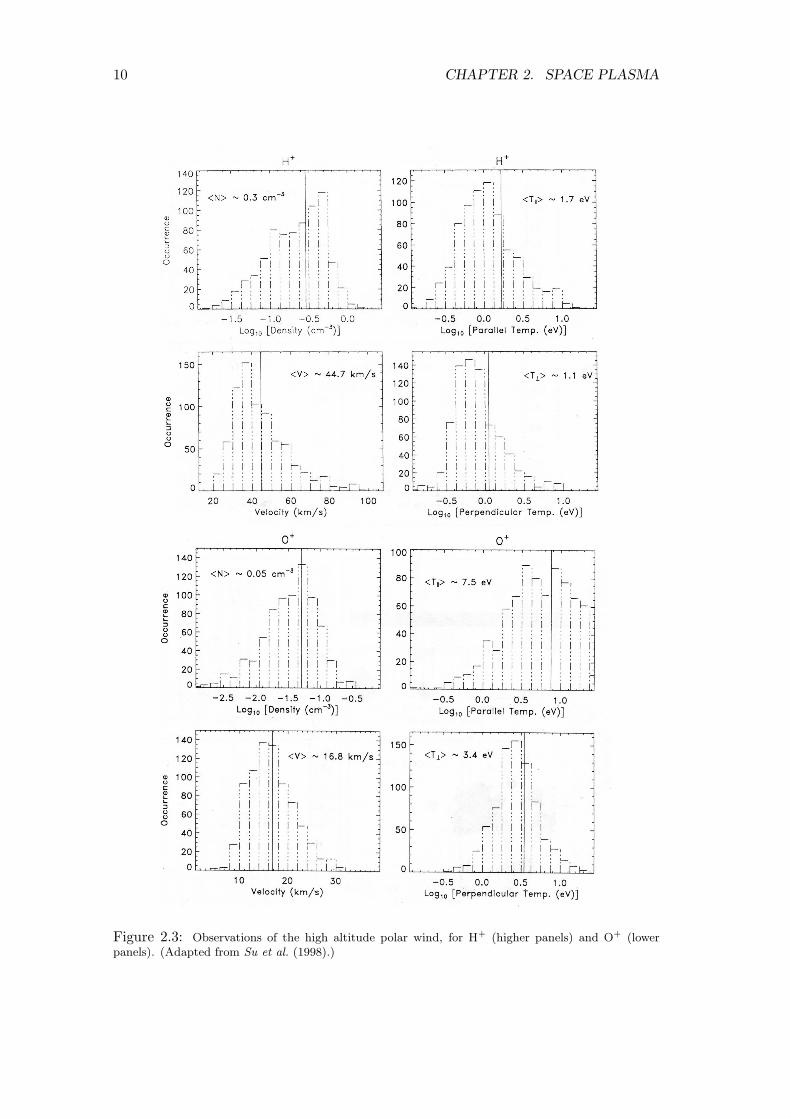
(apogee, northern hemisphere) and 5000 km (perigee, southern hemisphere). Figure2.3 illustrates the observed characteristics of the high altitude polar wind. These polarwind observations reveals a faster, hotter and more rich in O+ plasma than predictedby thermal outflow theories. The discrepancy between theory and observations wasinterpreted as a result of neglecting energy input in the topside auroral ionosphere(Moore et al., 1999). At 5000 km, the H+ are outflowing, but the mean velocity of O+

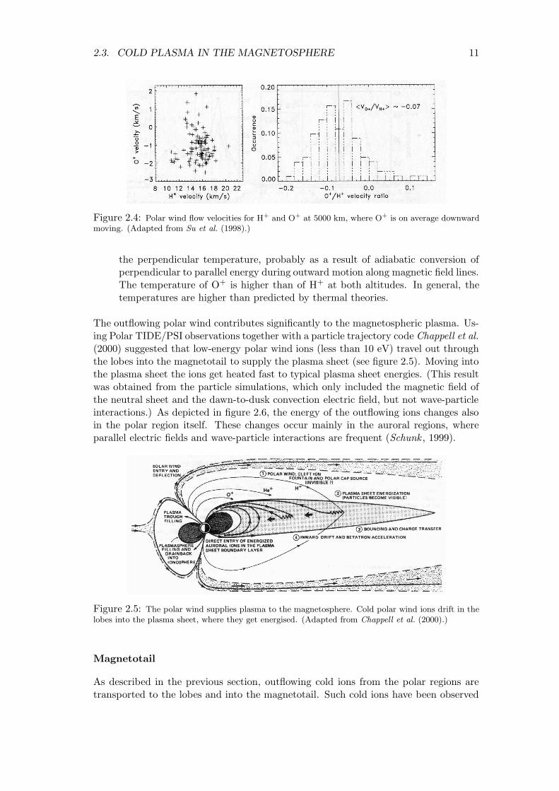
is directed downward (see figure 2.4). The high altitude O+ can thus not originate fromthe polar cap proper, but are transported into the polar cap from the dayside auroralzone by the cleft ion fountain (see section 2.3.1). Parts of the ion distribution are againtrapped in the Earth’s gravity field over the polar caps and flow downward.

The polar wind survey by Su et al. (1998) revealed the following parameters of thepolar wind:

Density At 5000 km the dominant ion species is O+ (nO+ ≈ 8 cm−3, nH+ ≈ 2 cm−3),whereas at 8 RE the plasma is totally dominated by H+ (nO+ ≈ 0.05 cm−3,nH+ ≈ 0.3 cm−3). He+ only constitutes a small fraction of the total number ofions at both altitudes.

Flow speeds The polar wind exhibits a wide variation in flow speeds with altitude:

• 5000 km: The H+ ions are supersonic and upflowing with an average speedof 15 km/s, while the O+ ions are subsonic and moving towards the earthwith an average speed of 1 km/s.

• 8 RE: Both H+ and O+ are supersonic and flowing upwards. The averagespeed for H+ is 45 km/s and for O+ 27 km/s.

Su et al. (1998) admit that the results at 8 RE are somewhat in contradictionwith polar wind models. We would like to stress that the discrepancy betweentheory and observations to some extent could be explained by the fact that thelowest detectable flow speed for cold hydrogen ions with Polar is 20 km/s. Thisspeed corresponds to a flow energy of 2 eV, which is the energy the ions need tosurmount the potential barrier of the spacecraft at 2 V. If many ions have flowspeeds below 20 km/s, which is expected from outflow theories and observationsat lower altitudes, the statistics in panel 2 (left) in figure 2.3 will be wrong andthe mean speed of hydrogen could be considerably smaller. This is not a problemfor O+ ions, since they are much more heavy. At 5000 km a large portion ofthe hydrogen ions are shielded as well, but these data has been corrected for thespacecraft potential using a bi-Maxwellian filling in procedure, explaining why itis possible to attain average velocities below 20 km/s.

Temperature At 5000 km the perpendicular temperatures are higher than the paralleltemperatures for both ion species, which may indicate perpendicular heating bywave-particle interactions. At 8 RE the parallel temperatures are higher than


Figure 2.3: Observations of the high altitude polar wind, for H+ (higher panels) and O+ (lowerpanels). (Adapted from Su et al. (1998).)


Figure 2.4: Polar wind flow velocities for H+ and O+ at 5000 km, where O+ is on average downwardmoving. (Adapted from Su et al. (1998).)

the perpendicular temperature, probably as a result of adiabatic conversion ofperpendicular to parallel energy during outward motion along magnetic field lines.The temperature of O+ is higher than of H+ at both altitudes. In general, thetemperatures are higher than predicted by thermal theories.

The outflowing polar wind contributes significantly to the magnetospheric plasma. Us-ing Polar TIDE/PSI observations together with a particle trajectory code Chappell et al.(2000) suggested that low-energy polar wind ions (less than 10 eV) travel out throughthe lobes into the magnetotail to supply the plasma sheet (see figure 2.5). Moving intothe plasma sheet the ions get heated fast to typical plasma sheet energies. (This resultwas obtained from the particle simulations, which only included the magnetic field ofthe neutral sheet and the dawn-to-dusk convection electric field, but not wave-particleinteractions.) As depicted in figure 2.6, the energy of the outflowing ions changes alsoin the polar region itself. These changes occur mainly in the auroral regions, whereparallel electric fields and wave-particle interactions are frequent (Schunk , 1999).

Figure 2.5: The polar wind supplies plasma to the magnetosphere. Cold polar wind ions drift in thelobes into the plasma sheet, where they get energised. (Adapted from Chappell et al. (2000).)

Magnetotail

As described in the previous section, outflowing cold ions from the polar regions aretransported to the lobes and into the magnetotail. Such cold ions have been observed


Figure 2.6: Schematic picture of different acceleration processes that can affect the polar wind.(Adapted from Schunk and Sojka (1997).)

in the lobes, the plasma sheet boundary layer (PSBL) and the plasma sheet (Etchetoand Saint-Marc, 1985; Seki et al., 2003; Sauvaud et al., 2004).

Seki et al. (2003) reported cold ions in the plasma sheet, which were exempted fromheating. The observations were made by the GEOTAIL spacecraft at positions from 8to 27 RE from the Earth. At the time of observation the spacecraft was in eclipse behindthe Earth, yielding a negative spacecraft potential as a result of inhibited photoelectronemission. The negative spacecraft potential allowed detection of all distributions of ions,regardless of temperature. The authors suggest that the cold ions may not have passedthrough the boundary heating region adjacent to the plasmasheet (the PSBL), buthave directly flown out from the ionosphere. However, the gradual filling of a magneticflux tube that has already passed the heating region would take several hours, whichis much longer than the transport of the flux tube predicted by ordinary magneticconvection theory. If this interpretation is correct, ionospheric outflow fluxes predictthat the conventional ideas of magnetospheric convection have to be reformulated.

In the PSBL Etcheto and Saint-Marc (1985) found ”anomalously” high plasma densities(around 5 cm−3) and low perpendicular energies (less than 30 eV) using measurementsfrom a relaxation sounder on board the two ISEE spacecraft. The origin of the coldand dense plasma was not possible to deduce in this study, but the authors give twopossible explanations:

1. Detachments from the plasmasphere: Cold plasmaspheric detachments are con-


vected into the nightside magnetotail.

2. Outflowing ions from polar regions: High density plasma in the polar ionospheresupplies the PSBL.

Sauvaud et al. (2004) have presented case studies of cold ions in the lobes, the plasmasheet and PSBL using the Cluster ion spectrometers (CIS). These ions have only beendetected for high drift velocities, when the drift energy is high enough to overcome thespacecraft potential barrier. The study confirms the idea of transport of ionosphericions into the magnetotail and show in particular that ions are massively injected fromthe nightside ionosphere into the tail during storms and substorms. One single injectioncan even account for over 80% of the plasma sheet O+ population. Furthermore, theobservations of a cold proton population inside the PSBL during quiet times precedinga substorm was reported. The cold ions are accelerated to several hundreds km/s as aresult of fast flows in the PSBL4, which allows to measure the density of this populationprecisely. The density of the cold population of around 0.1 cm−3 is almost comparableto the density of the hot plasma sheet ions, which reaches a maximum of 0.25 cm−3 inthis study. Other examples, where accelerated cold ions in the magnetotail have beenable to overcome the spacecraft potential barrier, are presented by Orsini et al. (1990)and Seki et al. (2002).

In Paper III (Engwall et al., 2006a), we report cold ions in the magnetotail lobes at18 RE measured simultaneously with two alternative methods: 1. Ion detectors incombination with artificial spacecraft potential control. 2. Deriving ion flow velocityfrom electric field instruments. As far as we know, this is the first study of flowproperties of low-energy ions below 50 eV beyond the Polar apogee of 8 RE.

Dayside magnetosphere

Plasmaspheric detachments can expel large amounts of cold dense plasma into thedayside magnetosphere. This has been observed by many spacecraft5. This plasmas-pheric plasma contributes to both microscale and macroscale physical processes. Re-cent observations with Polar (Chen and Moore, 2004) have revealed a large numberof plasmaspheric ions flowing with high velocity towards the subsolar magnetopause.These fast flows seem to occur predominantly at southward IMF, which may suggestthat they are related to the process of reconnection at the dayside magnetopause: theplasmaspheric detachment flows to fill the low density reconnection region, bringingits frozen in flux tubes towards the approaching solar wind, thus contributing to newreconnection processes.

Cold ions have also been observed by Cluster in the upper dayside magnetosphereadjacent to the magnetopause (Sauvaud et al., 2001). These ions became visible tothe ion instrument only when they were accelerated by intermittent motion of themagnetosphere. However, they were shown to exist at other times by simultaneous

4The occurrence of such fast flows in the PSBL can create Alfven perturbations in the lobe, whichhave also been observed in the present study by Sauvaud et al. (2004). The authors argues that theflows could also trigger Kelvin-Helmholtz instabilities.

5e.g. Ogo 4, 5, and 6, Ariel 3, ATS and LANL geostationary satellites (see Chen and Moore (2004),and references therein).


observations with the WHISPER6 experiment. The density of this cold ion populationwas found to be as high as 1 cm−3, which is much higher than the surrounding localdensity of ions.

6Whisper of HIgh frequency and Sounder for Probing Electron density by Relaxation (Decreau

et al., 2001).

Chapter 3

Probe measurements of plasma

Many plasma instruments, e.g. for measurements of electric fields, density and tem-perature, are based on the Langmuir probe theory (Mott-Smith and Langmuir , 1926).These instruments use probes, which collect particles from the ambient plasma. Tounderstand the functioning of the probe instruments, it is essential to quantify theparticle currents to the probe, which will be the subject of the following section. Forthe interested reader, we will give the derivations of these currents in detail. However,to be able to follow the rest of the thesis, it is only important to note that the currentsare exactly determined for spherical and cylindrical probes under certain conditionsand that the currents are dependent on plasma density and temperature as well ason probe potential. The probe theory is also the basis for understanding spacecraftcharging, which is treated in section 4.1.

3.1 Probe currents in Maxwellian plasmas

The quantification of the probe currents was first carried out theoretically by Mott-Smith and Langmuir (Mott-Smith and Langmuir , 1926) by using the orbital motionlimited theory (OML). This theory is not based on plasma physics, but regards adistribution of particles moving in the vacuum field from the probe, thus obtainingtrajectories determined only by conservation of energy and angular momentum. Thisapproach can be adopted when the radius of the probe is much smaller than the Debyelength. If the probe radius, on the contrary, is much larger than the Debye length, theprobe will be efficiently shielded and sheath limited theory (SL) must instead be used.In the following, we will only regard OML theory in unmagnetised plasmas and applyit to spherical probes, noting that it is fully developed also for cylinders.

Mott-Smith and Langmuir (1926) treat the currents to a probe in an isotropic plasma.As a starting point, they examine the random currents, which are the currents to a probeat zero potential, and then continue with the currents to a charged probe (see sections3.1.1 and 3.1.2). If the plasma is drifting with respect to the probe, the equations forthe currents have to be modified to the form given in section 3.1.3. In addition to thecurrents from the ambient plasma to the probe, the photoelectron current often getsimportant in space for sunlit probes (see section 3.1.4). In section 3.1.5, we describehow all the currents balance at a certain potential, which is called the floating potentialof the probe.

15

16 CHAPTER 3. PROBE MEASUREMENTS OF PLASMA

3.1.1 Random current

Consider a charged particle with orthonormal velocity components u, v and w at somedistance r from an uncharged spherical probe with radius a. The component u givesthe radial velocity, counted positive when directed towards the probe, while v and ware tangential velocity components. In a Maxwellian plasma the distribution functionis then given by

f(u, v, w) = n( m

2πKT

)3/2e−

m2KT

(u2+v2+w2), (3.1)

if we consider a region so far from the probe that absorption by the probe does notchange the plasma.

The number of particles per unit volume in the velocity range [u, u + du], [v, v + dv]and [w, w + dw] is

f(u, v, w) du dv dw = n( m

2πKT

)3/2e−

m2KT

(u2+v2+w2) du dv dw. (3.2)

Now, set p =√

v2 + w2. Then, v = p cos Ψ and w = p sinΨ, where Ψ = arctan ( wv )

(p ∈ [0,∞[ and Ψ ∈ [0, 2π[). This change of variables yields

f(u, v, w) du dv dw = g(u, p,Ψ)

∣

∣

∣

∣

∂(v, w)

∂(p,Ψ)

∣

∣

∣

∣

du dp dΨ = g(u, p,Ψ) p du dp dΨ, (3.3)

where

g(u, p,Ψ) = n( m

2πKT

)3/2e−

m2KT

(u2+p2). (3.4)

The current to the probe from the plasma is created by plasma particles hitting theprobe. Only particles with positive radial velocities, i.e. u ∈ [0,∞[, will reach theprobe and contribute to the current. Thus, the particle flux to the probe is

Φ =

∫ 2π

0

∫ ∞

0

∫ ∞

0u g(u, p,Ψ) p du dp dΨ = n

√

KT

2πm. (3.5)

The number of particles per second hitting a spherical surface, S, centred at the probeis then given by η = SΦ. The current to the probe is obtained by multiplying the aboveexpression by the particle charge, q, i.e. I = qη. At the surface of the probe S = 4πa2,which gives the final expression for the current:

I = 4πa2nq

√

KT

2πm= 2nqa2

√

2πKT

m≡ Ith. (3.6)

This is the random current to a probe in a Maxwellian plasma for the particle speciesof mass m and charge q.

3.1. PROBE CURRENTS IN MAXWELLIAN PLASMAS 17

3.1.2 Current to charged probe

In this section, we derive the current to a spherical probe charged to a potential Vp withrespect to the plasma. As described in section 2.2, the potential from a charged objectimmersed in a plasma will be shielded by charges of opposite sign. A negatively chargedobject will for example be shielded by a cloud of positive ions. The shielding particlestogether form a sheath, beyond which the potential from the object will not reach. Nowconsider a particle at the sheath edge, s, with charge q, radial velocity u and tangentialvelocity components v and w. As in the previous section v and w are replaced byp =

√v2 + w2 and the same transformation is performed for the distribution function:

f(u, v, w) du dv dw = g(u, p,Ψ) p du dp dΨ.

The probe current can be obtained through the particle flow to the probe, I = qSaΦa,where Sa is the surface area of the probe and Φa the particle flux to the probe at itssurface (r = a). As in the derivation of the random current, Φ(r) can be integratedfrom the distribution function. Inside the sheath, the plasma has been disturbed bythe potential from the probe, and the distribution function has to be derived fromLiouville’s theorem (Goldstein et al., 2002), which states that the distribution functionalong a particle trajectory is constant. If we can trace a particle from the sheath to theprobe surface, it is therefore possible to determine the current from the distributionfunction at s. Since the plasma is undisturbed outside the sheath, the distributionfunction at s is taken to be a common Maxwellian.

The tracing of the particles is performed by considering the principles of conservationof energy and angular momentum. If ua and pa are the radial and tangential velocitycomponents, respectively, for a particle arriving at the probe surface (r = a), we obtain

1

2m(u2 + p2) =

1

2m(u2

a + p2a) + qVp (energy) (3.7)

ps = paa (angular momentum), (3.8)

assuming zero potential at infinity.

Combining the equations yields

u2a = u2 −

(

s2

a2− 1

)

p2 − 2q

mVp (3.9)

pa =s

ap. (3.10)

To reach the probe the particle has to be approaching the probe, i.e. u > 0, since outsidethe sheath, there is no field that could attract the particle to the probe. Moreover, froma mathematical point of view, u2

a ≥ 0. Inserting the last condition into equation (3.9)leads to the following inequality for p:

p2 ≤ a2

s2 − a2

(

u2 − 2q

mVp

)

. (3.11)

Let p1 =√

a2

s2−a2

(

u2 − 2 qmVp

)

, so that the range of p is [0, p1]. Since p2 ≥ 0, inequality

(3.11) also leads to an additional condition for u: u2 ≥ 2 qmVp, which is automatically


satisfied for attractive potentials (qVp < 0). We thus have u ≥ u1, where u1 = 0 for

attractive potentials and u1 =√

2 qmVp for repulsive potentials. Now, we can calculate

the flux at r = s of particles which will eventually reach the probe and contribute tothe current:

Φ(s) =

∫ 2π

0

∫ ∞

u1

∫ p1

0u g(u, p,Ψ) p dp du dΨ =

= n

√

KT

2πme−

m2KT

u21

[

1 −(

s2 − a2

s2

)

exp

(

a2

s2 − a2

(

qVp

KT− m

2KTu2

1

))]

(3.12)

The current to the probe then is

I(s) = qSΦ(s)

= q4πs2n

√

KT

2πme−

m2KT

u21

[

1 −(

s2 − a2

s2

)

exp

(

a2

s2 − a2

(

qVp

KT− m

2KTu2

1

))]

(3.13)

Letting the sheath expand to infinity, equation (3.13) takes the form

I∞ = lims→∞

I(s) = 4πa2nq

√

KT

2πme−

m2KT

u21

(

1 − qVp

KT+

m

2KTu2

1

)

=

= Ithe−m

2KTu21

(

1 − qVp

KT+

m

2KTu2

1

)

(3.14)

In this limiting case there will be no shielding, which means that it corresponds to thecurrent to a probe in vacuum, i.e. the OML approximation. Inserting the values foru1, the current to the probe can be expressed as

I∞ =

Ith

(

1 − qVp

KT

)

(attractive potentials, qVp < 0)

Ithe−

qVp

KT (repulsive potentials, qVp > 0)

(3.15)

where Ith is the random current as shown in equation (3.6). When Vp = 0, I∞ = Ith

as expected.

3.1.3 Probe current in flowing plasma

Medicus (1961, 1962) treats the current to a probe in a flowing plasma. In this case, aparticle far away from the probe with velocity v and impact parameter d is considered(see figure 3.1). The particle is outside the sheath surrounding the probe, and thusfeels no electrical force. Furthermore, the sheath is assumed to be large compared to


the probe so that OML is applicable and all particles that enter the sheath will notreach the probe. This allows grazing incidence, which means that also particles withzero radial velocity at the probe surface contribute to the current.1

Figure 3.1: Probe in a flowing plasma. The velocity outside the sheath is v, which can be decomposedinto the radial component u and the tangential component p. The sheath is assumed to be much largerthan the probe. d is the impact parameter.

Since no fields are present outside the sheath, the velocity at the sheath edge is v (thesame as far away from the probe). Let u and p be the radial and tangential velocitycomponents respectively of v. The velocities at the probe surface (r = a) are denotedby subscript a.

As before, the constraints are set up by the principles of conservation of energy andangular momentum:

1

2m(u2 + p2) =

1

2m(u2

a + p2a) + qVp (energy) (3.16)

paa = ps = vd (angular momentum) (3.17)

In the case of grazing incidence, we have ua = 0 and the limiting impact parameter, dg,is then given by

d2g = a2

(

1 − 2qVp

mv2

)

. (3.18)

For repulsive potentials qVp is positive, which means that there is a lower limit on v,since d2

g > 0. In other words, the velocity of the particle has to be sufficiently highto enable it to overcome the potential barrier and reach the probe. This lower limit isgiven by

1This is a simplified treatment compared to Medicus, who also treats the sheath limited case, whereany particle entering the sheath will reach the probe.


v1 =

√

2qVp

m. (3.19)

For accelerating potentials d2g is positive for any v ∈ [0,∞[. All particles with a smaller

impact parameter than dg will reach the probe. The current to the probe is then givenby the flow through the circle with radius dg:

dI = πd2gqvF (v)dv,

= πa2q

(

1 − 2qVp

mv2

)

v F (v) dv

(3.20)

I = πa2q

∫ ∞

v1

(

1 − 2qVp

mv2

)

v F (v) dv, (3.21)

where n is the number density, F (v) the speed distribution2 and v1 the minimumspeed, which is 0 for accelerating potentials and given by equation (3.19) for repulsivepotentials. For a drifting plasma with zero temperature, F (v) = nδ(v − vd), where vd

is the drift velocity. The current is then

I = πa2qn

∫ ∞

v1

(

1 − 2qVp

mv2

)

vδ(v − vd) dv =

πa2qnvd

(

1 − 2qVp

mv2d

)

(vd ≥ v1)

0 (vd < v1)

(3.22)

The first result holds for all accelerating potentials and for repulsive potentials whenthe drift velocity is larger than v1. It is interesting to compare the equations to acharged probe in a non-drifting Maxwellian plasma (equation (3.15)) with equation(3.22). For the attractive potential, the functional forms are identical, with the driftenergy 1

2mv2d replacing the thermal energy KT and πa2qnvd replacing the random

current 4πa2qn√

KT2πm , which is easy to understand from a basic consideration of the

situation. In the random current, the thermal velocity√

KT2πm is replaced by the drift

velocity vd and 4πa2 is replaced by πa2, since for the flowing plasma a probe at zeropotential collects current only from one direction. For repulsive potentials, equation(3.22) is actually consistent with the limit T → 0 of (3.15).

In the case of a drifting Maxwellian plasma the three dimensional velocity distributionis given by

f(vx, vy, vz) = n( m

2πKT

)32e−

m2KT

[v2x+v2

y+(vz−vd)2] (3.23)

2It may at first seem counterintuitive that we can use a scalar argument v in the distribution functionF (v), since the drift clearly produces an anisotropy. However, there is no feedback from the particledistribution on the fields in the OML limit, and therefore the anisotropy is not important for the totalcurrent to the probe. To put it simply, the probe doesn’t care about what direction the particle arrivesfrom. If plasma effects are important, the sheath becomes anisotropic and the present analysis doesnot hold.


for a drift in the z-direction with velocity vd. Changing to spherical coordinates we get

f(v, θ, φ) = n( m

2πKT

)32e−

m2KT

[v2+v2d−2vvd cos θ] (3.24)

The speed distribution is

F (v) =

∫ π

0

∫ 2π

0f(v, θ, φ) v2 sin θ dφ dθ

= 2n

√

m

2πKT

v

vde−

m2KT

[v2+v2d] sinh

mvvd

KT

(3.25)

Inserting equation (3.25) into equation (3.21) yields

I = qna

√

2πKT

m

[

e−m

2KT(v2

1+v2d)

(

v1

vdsinh

(mvdv1

KT

)

+ cosh(mvdv1

KT

)

)

+

√

KT

2mv2d

(

mv2d

KT+ 1 − 2qVp

KT

)

E

(√

m

2KT(v1 − vd),

√

m

2KT(v1 + vd)

)

]

(3.26)

where E(a, b) =∫ ba e−y2

dy. In the limit vd → 0, equation (3.26) reduces to

I = qna

√

2πKT

me−

m2KT

v21

(

mv21

KT− 2qVp

KT+ 2

)

. (3.27)

Inserting v1 = 0 for accelerating potentials and v1 =√

2qVp

m for repulsive potentials, we

retrieve the classical Langmuir results for a non-drifting plasma (see equation (3.15)).For large drift velocities (vd → ∞) both the ion and electron current will approachqna2πvd and the total current will thus vanish.

3.1.4 Photoelectron current

For sunlit probes, in addition to plasma ion and electron currents, we have to regardthe photoelectron current3. In magnetospheric plasmas the photoelectron current isdominating, which brings the probe to a positive potential. The photoelectron currentdepends on the projected area of the probe to the sun, Ap, the surface propertiesof the probe, local plasma conditions, distance to the Sun and the solar spectrum.Because of these different dependences, there are many different expressions used forthe photoelectron current. Pedersen (1995) has used measurements to fit an analyticalexpression to satellite data. In this treatment, we adopt the theoretical expressions forspherical probes derived by Grard (1973).

For negative potentials all photoelectrons can escape from the probe and the photoelec-tron current will be saturated at the constant value I 0

ph:

3In a rigorous treatment other effects, such as secondary electron emission, should also be treated(Garrett , 1981; Eriksson et al., 1999). These currents are mentioned in section 4.1.


Iph = I0ph = Apj

0ph, Vp < 0 (3.28)

where j0ph is the photoelectron current density, which has to be estimated from satellite

data. The current density shows large variations and can be in the range j 0ph = 1.5 −

8 nA cm−2 for a probe operating in space for a long period (Laakso et al., 1995, andreferences therein).

Probes at positive potentials will recollect some of the photoelectrons, the more thehigher the potential is. The photoelectron current for a spherical probe at positivepotential can be approximated by the analytic function (Grard , 1973)

Iph = I0ph

(

1 +eV

KTph

)

exp− eV

KTphVp < 0, (3.29)

assuming that the probe is smaller than the Debye length and that the photoelectrondistribution is Maxwellian. Tph is the photoelectron temperature, which is of the orderof 1.5 eV.

3.1.5 Current balance

Combining the photoelectron current with the expressions for the electron and ioncurrents, current-voltage relations for the probes can be derived. At equilibrium, thecurrents will balance each other (

∑

n In = Ie+Ii+Iph = 0) and the probe will attain itsfloating potential. For sunlit probes operating above Earth’s ionosphere, the ion currentis negligible and the floating potential is in practice obtained by balancing the currentof escaping photoelectrons and impinging plasma electrons. In the magnetosphere, thefloating potential is normally a few volts positive (Pedersen et al., 1984). Figure 3.2shows the current balance for ambient plasma electrons (blue) and escaping photoelec-trons (red) to a probe (radius 4 cm) in a magnetospheric plasma of temperature 10 eVand density 10 cm−3. The photoelectron current density is assumed to be 6 nAcm−2.The currents balance each other at approximately 9.3 V positive.

For a probe in shadow, the situation becomes very different. In this case the probe willbe at negative potential and if the ion and electron temperatures are equal the currentbalance equation reduces to

Mex + x − 1 = 0, (3.30)

where x = eVp/KTe and M =√

mi/me, me and mi being the electron and ion massrespectively. The numerical solution of the equation is x = eVp/KTe ≈ −2.5. Thenegative potential can be explained by the fact that, when the electron and ion tem-peratures are equal, the electrons will move faster than the ions and thus hit the probemore frequently.

3.2 Probe measurements of densities and temperatures

Langmuir probes have been used for measurements of among other plasma densities,temperatures and electric fields in space since the beginning of the space era, and

3.3. ELECTRIC FIELD MEASUREMENTS WITH DOUBLE PROBES 23

2 4 6 8 10 12 14 16 18 20−120

−100

−80

−60

−40

−20

0

20

Probe potential [V]

Cur

rent

[nA

]

Floating potential:8.3 V

Ambient electron currentPhotoelectron current

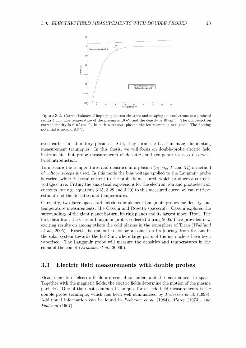
Figure 3.2: Current balance of impinging plasma electrons and escaping photoelectrons to a probe ofradius 4 cm. The temperature of the plasma is 10 eV and the density is 10 cm−3. The photoelectroncurrent density is 6 nAcm−2. In such a tenuous plasma the ion current is negligible. The floatingpotential is around 8.3 V.

even earlier in laboratory plasmas. Still, they form the basis in many dominatingmeasurement techniques. In this thesis, we will focus on double-probe electric fieldinstruments, but probe measurements of densities and temperatures also deserve abrief introduction.

To measure the temperatures and densities in a plasma (ni, ne, Ti and Te) a methodof voltage sweeps is used. In this mode the bias voltage applied to the Langmuir probeis varied, while the total current to the probe is measured, which produces a current-voltage curve. Fitting the analytical expressions for the electron, ion and photoelectroncurrents (see e.g. equations 3.15, 3.28 and 3.29) to this measured curve, we can retrieveestimates of the densities and temperatures.

Currently, two large spacecraft missions implement Langmuir probes for density andtemperature measurements: the Cassini and Rosetta spacecraft. Cassini explores thesurroundings of the giant planet Saturn, its ring planes and its largest moon Titan. Thefirst data from the Cassini Langmuir probe, collected during 2005, have provided newexciting results on among others the cold plasma in the ionosphere of Titan (Wahlundet al., 2005). Rosetta is sent out to follow a comet on its journey from far out inthe solar system towards the hot Sun, where large parts of the icy nucleus have beenvaporised. The Langmuir probe will measure the densities and temperatures in thecoma of the comet (Eriksson et al., 2006b).

3.3 Electric field measurements with double probes

Measurements of electric fields are crucial to understand the environment in space.Together with the magnetic fields, the electric fields determine the motion of the plasmaparticles. One of the most common techniques for electric field measurements is thedouble probe technique, which has been well summarised by Pedersen et al. (1998).Additional information can be found in Pedersen et al. (1984), Mozer (1973), andFahleson (1967).


3.3.1 Measurement technique

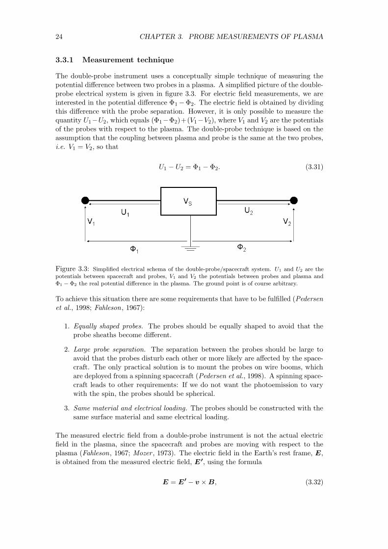
The double-probe instrument uses a conceptually simple technique of measuring thepotential difference between two probes in a plasma. A simplified picture of the double-probe electrical system is given in figure 3.3. For electric field measurements, we areinterested in the potential difference Φ1 −Φ2. The electric field is obtained by dividingthis difference with the probe separation. However, it is only possible to measure thequantity U1−U2, which equals (Φ1−Φ2)+(V1−V2), where V1 and V2 are the potentialsof the probes with respect to the plasma. The double-probe technique is based on theassumption that the coupling between plasma and probe is the same at the two probes,i.e. V1 = V2, so that

U1 − U2 = Φ1 − Φ2. (3.31)

Figure 3.3: Simplified electrical schema of the double-probe/spacecraft system. U1 and U2 are thepotentials between spacecraft and probes, V1 and V2 the potentials between probes and plasma andΦ1 − Φ2 the real potential difference in the plasma. The ground point is of course arbitrary.

To achieve this situation there are some requirements that have to be fulfilled (Pedersenet al., 1998; Fahleson, 1967):

1. Equally shaped probes. The probes should be equally shaped to avoid that theprobe sheaths become different.

2. Large probe separation. The separation between the probes should be large toavoid that the probes disturb each other or more likely are affected by the space-craft. The only practical solution is to mount the probes on wire booms, whichare deployed from a spinning spacecraft (Pedersen et al., 1998). A spinning space-craft leads to other requirements: If we do not want the photoemission to varywith the spin, the probes should be spherical.

3. Same material and electrical loading. The probes should be constructed with thesame surface material and same electrical loading.

The measured electric field from a double-probe instrument is not the actual electricfield in the plasma, since the spacecraft and probes are moving with respect to theplasma (Fahleson, 1967; Mozer , 1973). The electric field in the Earth’s rest frame, E,is obtained from the measured electric field, E

′, using the formula

E = E′ − v × B, (3.32)


where v is the velocity of the satellite in the Earth system and B is the Earth’s magneticfield. This means that for measurements of the electric field in a frame of referenceindependent of the spacecraft motion, we also need detailed measurements of v and B.For a rotating spacecraft with radially deployed probes, it is the spin plane component ofthe electric field that is measured. To obtain the full electric field vector, it is normallya good assumption to take E⊥ � E‖, at least for quasi-DC fields. If B is not too closeto the spin plane, the total field can be constructed from the spin plane componentand the relation E · B = 0. One double-probe system on a spinning spacecraft isthus normally sufficient to determine the full electric field vector. However, it will takeone spin period, which will prevent measurements of rapidly varying electric fields. Iftwo double-probes are used instead, the total electric field vector can be determinedimmediately and the only limitation is probe function and telemetry (Pedersen et al.,1998).

For measurements in a dense plasma the electron and ion currents are sufficiently highto give a good coupling between probe and plasma. In a tenuous plasma, photoemissionis essential for satisfactory probe-plasma coupling, which means that the probes haveto be sunlit to function. As can be seen in figure 3.2, the probes float at a relativelyhigh potential where the slope of the photoelectron current is small. This means thata small spurious current to one of the probes can result in a large false electric field.It is therefore desirable to bring the probe closer to the plasma potential, where thecurrent-voltage curve is steeper, which can be achieved by applying a bias current fromthe probe to the spacecraft (see figure 3.4).

Figure 3.4: The double-probe instrument in different environments: a) The ionosphere, b) Themagnetosphere, c) The magnetosphere with bias current. The bias current brings the probe potentialcloser to the plasma potential, where small spurious currents will not influence the potential of theprobe. (Adapted from Pedersen et al. (1998))

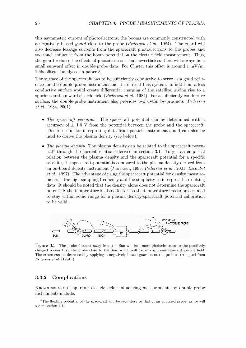
Even though the photoemission provide the necessary coupling between probe andplasma, it also introduces new errors in the measurement: If the booms are at the samepotential as the spacecraft, which is normally the case, the probe furthest away fromthe Sun will lose more photoelectrons to the booms than the probe closest to the Sun(see figure 3.5). This phenomenon creates a spurious sunward electric field. To reduce


this asymmetric current of photoelectrons, the booms are commonly constructed witha negatively biased guard close to the probe (Pedersen et al., 1984). The guard willalso decrease leakage currents from the spacecraft photoelectrons to the probes andtoo much influence from the boom potential on the electric field measurement. Thus,the guard reduces the effects of photoelectrons, but nevertheless there will always be asmall sunward offset in double-probe data. For Cluster this offset is around 1 mV/m.This offset is analysed in paper 3.

The surface of the spacecraft has to be sufficiently conductive to serve as a good refer-ence for the double-probe instrument and the current bias system. In addition, a lessconductive surface would create differential charging of the satellite, giving rise to aspurious anti-sunward electric field (Pedersen et al., 1984). For a sufficiently conductivesurface, the double-probe instrument also provides two useful by-products (Pedersenet al., 1984, 2001):

• The spacecraft potential. The spacecraft potential can be determined with aaccuracy of ± 1.0 V from the potential between the probe and the spacecraft.This is useful for interpreting data from particle instruments, and can also beused to derive the plasma density (see below).

• The plasma density. The plasma density can be related to the spacecraft poten-tial4 through the current relations derived in section 3.1. To get an empiricalrelation between the plasma density and the spacecraft potential for a specificsatellite, the spacecraft potential is compared to the plasma density derived froman on-board density instrument (Pedersen, 1995; Pedersen et al., 2001; Escoubetet al., 1997). The advantage of using the spacecraft potential for density measure-ments is the high sampling frequency and the simplicity to interpret the resultingdata. It should be noted that the density alone does not determine the spacecraftpotential: the temperature is also a factor, so the temperature has to be assumedto stay within some range for a plasma density-spacecraft potential calibrationto be valid.

Figure 3.5: The probe furthest away from the Sun will lose more photoelectrons to the positivelycharged booms than the probe close to the Sun, which will cause a spurious sunward electric field.The errors can be decreased by applying a negatively biased guard near the probes. (Adapted fromPedersen et al. (1984).)

3.3.2 Complications

Known sources of spurious electric fields influencing measurements by double-probeinstruments include:

4The floating potential of the spacecraft will be very close to that of an unbiased probe, as we willsee in section 4.1.


1. Asymmetries of the probes.

2. Coupling between probes and boom tips.

3. Wake effects.

4. Magnetisation.

5. Plasma density gradients.

How to prevent effects of the two first causes has already been treated in the previoussection. The influence of wakes is covered in section 5.3.

Magnetisation could complicate the measurements, when the electron gyroradius iscomparable to or smaller than the probe dimensions (Fahleson, 1967). In such a case,the probes will mostly collect electrons from a column parallel to the magnetic field.Gradients in the plasma density along the boom direction will cause spurious electricfields, since the basis of the assumption V1 = V2 is that the plasma is homogeneous.This error can be reduced by applying an appropriate bias current (Laakso et al., 1995).

A problem with a spinning double-probe system, not related to spurious electric fields,is that we are able to measure the parallel electric field only when the spin axis isperpendicular to B. In many cases it would also be interesting to measure parallellelectric fields (Fahleson, 1967), e.g. in the auroral acceleration regions.

Chapter 4

Spacecraft-Plasma Interactions

Spacecraft interact with the particles in the surrounding plasma, which has many con-sequences for both the spacecraft itself and the plasma environment. One of the phe-nomena of great importance is spacecraft charging. Another effect, which has alreadybeen mentioned briefly in connection with complications for double-probe electric fieldinstruments, is wakes behind spacecraft.

4.1 Spacecraft charging

The area of spacecraft charging has been subject to extensive research, especially forcommercial satellites, since the potential of a spacecraft in a dense plasma with veryenergetic (∼ 10 keV) electrons can reach high negative values on the order of kV. Ifthe spacecraft is charged unevenly, hazardous electrostatic discharges between differentparts of the spacecraft may occur, which will affect the performance of the satellite. Theproblem of uneven charging can often be solved by using a conductive surface on thespacecraft. Nevertheless, spacecraft charging and discharges remain an issue, especiallyfor certain elements, which for some reason are isolated, and for specifically vulnerableparts of the spacecraft, such as solar panels. The term spacecraft charging has mainlybeen attributed to cases with high negative potentials. In this section we will treat theprocess behind all types of charging of spacecraft, regardless of the resulting potential.

What makes the spacecraft charge at all? The process of spacecraft charging can beunderstood by probe theory: we just exchange the probe for the much larger space-craft and the qualitative picture of currents to the probe/spacecraft remains the same.However, we have no exact analytical expression for the currents in this case, sincespacecraft seldom are perfectly spherical or cylindrical. To get quantitative estimatesof the spacecraft charging level we therefore have to go to numerical simulations.

As we saw for the probes, an object immersed in a plasma will be hit by the plasmaparticles due to their thermal motion. The particles are collected by the object, andat thermal equilibrium it will become negatively charged, since the electron currentexceeds the ion current at zero potential and equal ion and electron temperatures. Thiscan be explained by the fact that ions and electrons have the same energy at thermalequilibrium, but the electrons move faster, because of their much lower mass. Thisresults in the electrons hitting the probe more frequently, leading to a net negativecharge. As was stated in section 3.1.4, photoemission is important in sunlit parts

28

4.2. WAKE EFFECTS 29

of the magnetosphere. There exist also further charging effects, which can becomeimportant in special cases. Including these additional charging effects, the currentbalance equation (see section 3.1.5) takes the form

∑

n

In = Ie + Ii + Ibse + Ise + Isi + Iph + Ib = 0. (4.1)

Ie, Ii and Iph are, as in the probe case, the electron, ion and photoelectron current,respectively. The term Ibse is the current of backscattered electrons due to Ie. The cur-rents Ise and Isi consist of secondary electrons, emitted when electrons and ions hit thespacecraft.1 In most cases for sunlit magnetospheric spacecraft, the secondary electronemission is negligible compared to the photoelectron current Iph. In sunlit magneto-spheric plasmas, the photoelectron current will be dominant over all other currentsand the spacecraft will reach a positive potential, where most of the photoelectrons arerecollected by the spacecraft, and it is only the small fraction of high energy photo-electrons escaping into the ambient plasma that will establish an equilibrium with theother currents (Torkar et al., 1998). Ib, finally, is the current from a possible active ionsource installed on the spacecraft, which is used for example for propulsion or potentialcontrol. An example is the potential control device on-board Cluster, called ASPOC2

(Torkar et al., 2001), which operates successfully to reduce the several tens of voltspositive spacecraft potential to constant values of a few volts. The potential controlmakes it possible to measure low energy ions. In addition to these currents, there couldalso be currents between adjacent surfaces, if they are charged to different potentials.One may also have to consider displacement currents for time-dependent problems.

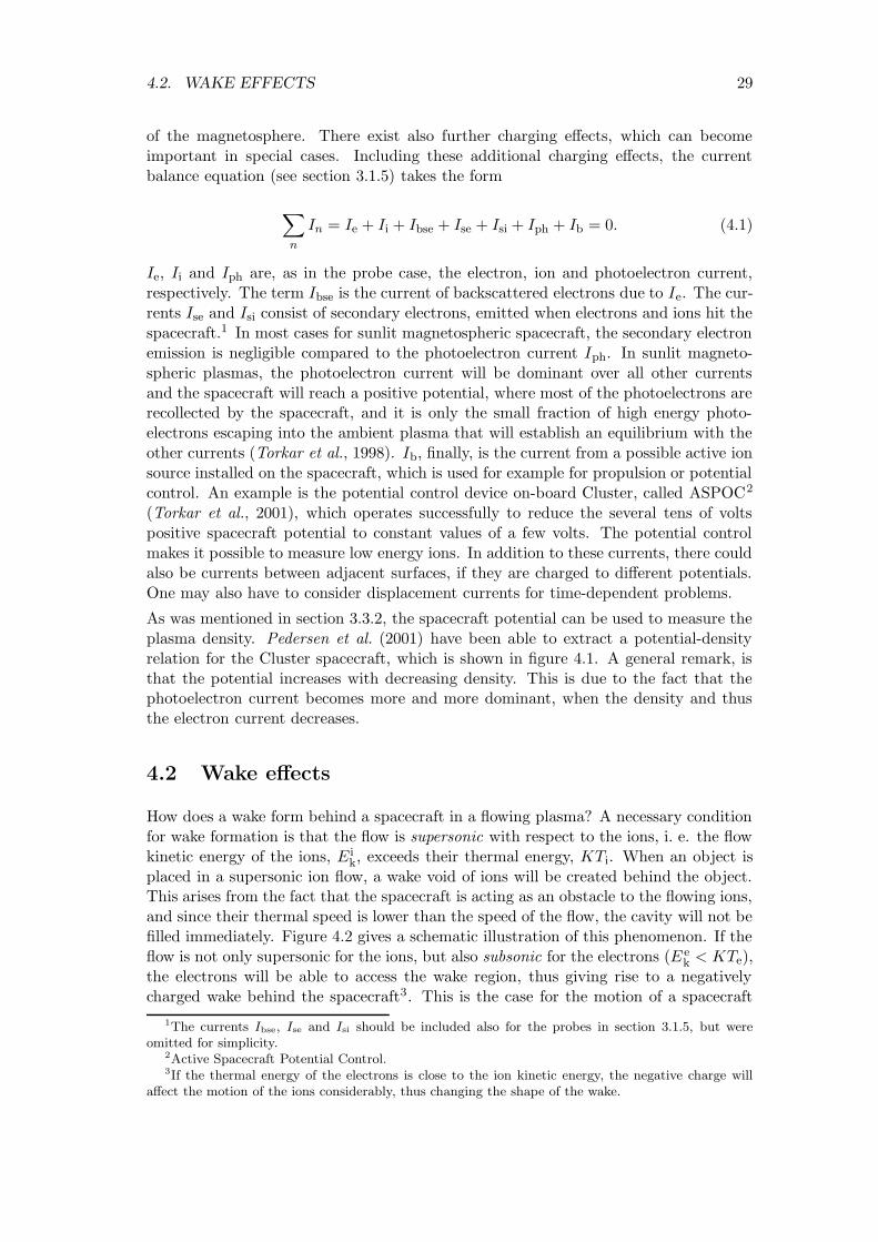
As was mentioned in section 3.3.2, the spacecraft potential can be used to measure theplasma density. Pedersen et al. (2001) have been able to extract a potential-densityrelation for the Cluster spacecraft, which is shown in figure 4.1. A general remark, isthat the potential increases with decreasing density. This is due to the fact that thephotoelectron current becomes more and more dominant, when the density and thusthe electron current decreases.

4.2 Wake effects

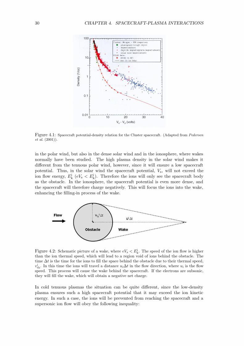
How does a wake form behind a spacecraft in a flowing plasma? A necessary conditionfor wake formation is that the flow is supersonic with respect to the ions, i. e. the flowkinetic energy of the ions, E i

k, exceeds their thermal energy, KTi. When an object isplaced in a supersonic ion flow, a wake void of ions will be created behind the object.This arises from the fact that the spacecraft is acting as an obstacle to the flowing ions,and since their thermal speed is lower than the speed of the flow, the cavity will not befilled immediately. Figure 4.2 gives a schematic illustration of this phenomenon. If theflow is not only supersonic for the ions, but also subsonic for the electrons (E e

k < KTe),the electrons will be able to access the wake region, thus giving rise to a negativelycharged wake behind the spacecraft3. This is the case for the motion of a spacecraft

1The currents Ibse, Ise and Isi should be included also for the probes in section 3.1.5, but wereomitted for simplicity.

2Active Spacecraft Potential Control.3If the thermal energy of the electrons is close to the ion kinetic energy, the negative charge will

affect the motion of the ions considerably, thus changing the shape of the wake.

30 CHAPTER 4. SPACECRAFT-PLASMA INTERACTIONS

Figure 4.1: Spacecraft potential-density relation for the Cluster spacecraft. (Adapted from Pedersen

et al. (2001)).

in the polar wind, but also in the dense solar wind and in the ionosphere, where wakesnormally have been studied. The high plasma density in the solar wind makes itdifferent from the tenuous polar wind, however, since it will ensure a low spacecraftpotential. Thus, in the solar wind the spacecraft potential, Vs, will not exceed theion flow energy, E i

k (eVs < Eik). Therefore the ions will only see the spacecraft body

as the obstacle. In the ionosphere, the spacecraft potential is even more dense, andthe spacecraft will therefore charge negatively. This will focus the ions into the wake,enhancing the filling-in process of the wake.

Figure 4.2: Schematic picture of a wake, where eVs < Eik. The speed of the ion flow is higher

than the ion thermal speed, which will lead to a region void of ions behind the obstacle. Thetime ∆t is the time for the ions to fill the space behind the obstacle due to their thermal speed,vith. In this time the ions will travel a distance ui∆t in the flow direction, where ui is the flow

speed. This process will cause the wake behind the spacecraft. If the electrons are subsonic,they will fill the wake, which will obtain a negative net charge.

In cold tenuous plasmas the situation can be quite different, since the low-densityplasma ensures such a high spacecraft potential that it may exceed the ion kineticenergy. In such a case, the ions will be prevented from reaching the spacecraft and asupersonic ion flow will obey the following inequality:

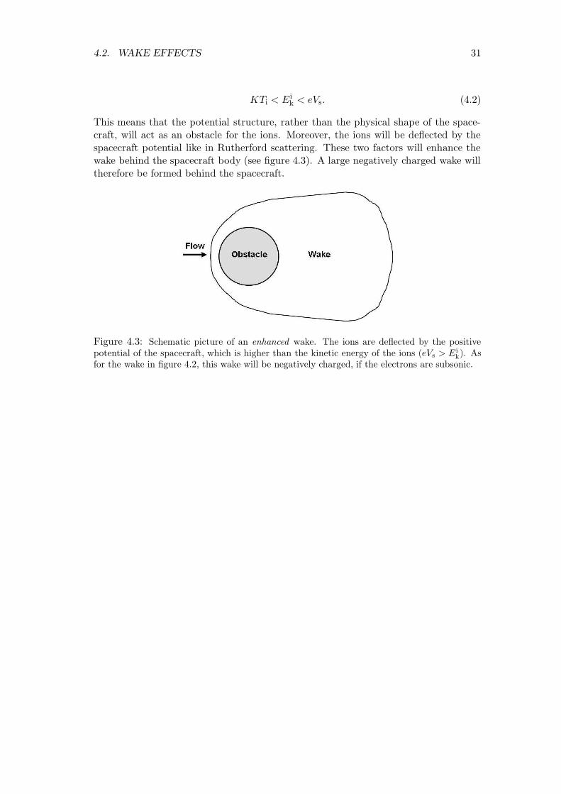
4.2. WAKE EFFECTS 31

KTi < Eik < eVs. (4.2)

This means that the potential structure, rather than the physical shape of the space-craft, will act as an obstacle for the ions. Moreover, the ions will be deflected by thespacecraft potential like in Rutherford scattering. These two factors will enhance thewake behind the spacecraft body (see figure 4.3). A large negatively charged wake willtherefore be formed behind the spacecraft.

Figure 4.3: Schematic picture of an enhanced wake. The ions are deflected by the positivepotential of the spacecraft, which is higher than the kinetic energy of the ions (eVs > Ei

k). Asfor the wake in figure 4.2, this wake will be negatively charged, if the electrons are subsonic.

Chapter 5

Wake effects in Cluster electric

field data

5.1 The Cluster satellites

The Cluster mission consists of four identical scientific spacecraft investigating space-and time-varying phenomena in the Earth’s magnetosphere (Escoubet et al., 2001). In1996 the first four Cluster satellites (Cluster I mission) were launched with the firstAriane-5 rocket. Unfortunately, this mission met a premature end, when the rocketexploded only 37 seconds after launch. The second attempt in the summer of 2000was more successful and the Cluster II mission has now been fully operational for morethan five years, and the mission has been extended four years until the end of 2009.The Cluster mission is regarded as a key mission for the European Space Agency, ESA,and has up to date provided a vast range of revealing data.

Figure 5.1: An artistic impression of the four Cluster satellites (from http://sci.esa.int).

The four satellites are orbiting the Earth in a formation, which is tetrahedral for as large

32

5.2. ELECTRIC FIELD MEASUREMENTS FROM CLUSTER 33

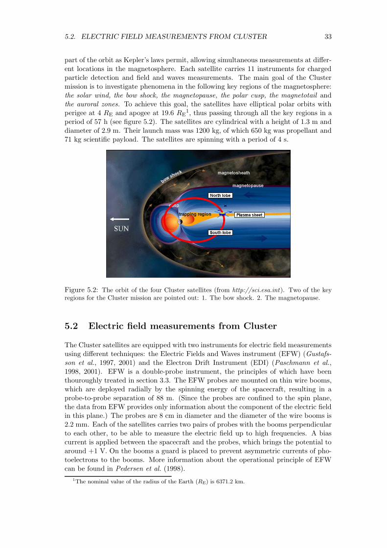
part of the orbit as Kepler’s laws permit, allowing simultaneous measurements at differ-ent locations in the magnetosphere. Each satellite carries 11 instruments for chargedparticle detection and field and waves measurements. The main goal of the Clustermission is to investigate phenomena in the following key regions of the magnetosphere:the solar wind, the bow shock, the magnetopause, the polar cusp, the magnetotail andthe auroral zones. To achieve this goal, the satellites have elliptical polar orbits withperigee at 4 RE and apogee at 19.6 RE

1, thus passing through all the key regions in aperiod of 57 h (see figure 5.2). The satellites are cylindrical with a height of 1.3 m anddiameter of 2.9 m. Their launch mass was 1200 kg, of which 650 kg was propellant and71 kg scientific payload. The satellites are spinning with a period of 4 s.

Figure 5.2: The orbit of the four Cluster satellites (from http://sci.esa.int). Two of the keyregions for the Cluster mission are pointed out: 1. The bow shock. 2. The magnetopause.

5.2 Electric field measurements from Cluster

The Cluster satellites are equipped with two instruments for electric field measurementsusing different techniques: the Electric Fields and Waves instrument (EFW) (Gustafs-son et al., 1997, 2001) and the Electron Drift Instrument (EDI) (Paschmann et al.,1998, 2001). EFW is a double-probe instrument, the principles of which have beenthouroughly treated in section 3.3. The EFW probes are mounted on thin wire booms,which are deployed radially by the spinning energy of the spacecraft, resulting in aprobe-to-probe separation of 88 m. (Since the probes are confined to the spin plane,the data from EFW provides only information about the component of the electric fieldin this plane.) The probes are 8 cm in diameter and the diameter of the wire booms is2.2 mm. Each of the satellites carries two pairs of probes with the booms perpendicularto each other, to be able to measure the electric field up to high frequencies. A biascurrent is applied between the spacecraft and the probes, which brings the potential toaround +1 V. On the booms a guard is placed to prevent asymmetric currents of pho-toelectrons to the booms. More information about the operational principle of EFWcan be found in Pedersen et al. (1998).

1The nominal value of the radius of the Earth (RE) is 6371.2 km.

34 CHAPTER 5. WAKE EFFECTS IN CLUSTER ELECTRIC FIELD DATA

Electron drift instruments are based on a technique determining the drift of high-energetic electrons in a magnetised plasma (see figure 5.3). Two beams of keV electronsare emitted from electron guns on the spacecraft. If a sufficiently strong (at least 30 nT)magnetic field is present, the electrons will experience a magnetic force strong enoughto make it possible to regain the electrons at detectors on the spacecraft. The electronswill also feel a force from the electric field in the plasma, which will lead to a drift ofthe electrons at a velocity of E ×B/B2 (see section 2.2). Detecting this drift from thetwo electron beams, the electric field can be extracted from magnetic field data.

Figure 5.3: The Electron Drift Instrument uses the drift of electrons in a magnetised plasmato measure the electric field Two high energetic electron beams are emitted from the spacecraftto measure the drift. (Adapted from Paschmann et al. (2001)).

Both of the instruments experience problems in some regions of the magnetosphere.Fortunately, the problems occur in different regions for the two instruments, makingthem complement each other well. An extensive comparison between EDI and EFWhas recently been carried out by Eriksson et al. (2006a). In short, EDI will evidentlynot function for too weak magnetic fields. It will also have problems for rapidly vary-ing magnetic and electric fields, which can be encountered for example in the auroraregions. In these regions, EDI often also have problems with naturally accelerated au-roral electrons of keV energy swamping the EDI detectors, thus making it impossibleto identify the emitted beam electrons. EFW will have no problems in these regions,due to the construction with two spinning crossing booms, which allow high frequencymeasurements. On the other hand, EFW measurements can be affected by the influenceof the positive potential of the satellite on the plasma environment. This is especiallythe case in cold, tenuous plasmas, where enhanced wakes may form.

5.3 Influence of wake on Cluster EFW

Comparisons with electron drift instruments on different spacecraft have shown thatformation of a wake behind the spacecraft and booms can severely affect the measure-ment from double probe instruments (Pedersen et al., 1984; Bauer et al., 1983; Erikssonet al., 2006a). The plasma is in most cases flowing perpendicular to the ambient electricfield (in the E × B direction and also parallel to B), which means that the spurious

5.3. INFLUENCE OF WAKE ON CLUSTER EFW 35

wake electric field will be in this direction, i.e. transverse to the real ambient electricfield (assuming the parallel electric fields are negligible).The wake will thus normallyhave more influence on the direction than of the amplitude of the measured transverseelectric field. However, the wake induced field along B may be many orders of magni-tude above any real parallel electric field. This is the case in e.g. the polar wind, wherespurious electric fields due to wakes have been observed in Cluster data (Eriksson et al.,2006a).

Wakes behind Cluster are common in the double-probe data, both in the solar wind andin outflowing cold tenuous plasma with ionospheric origin. As was described in section4.2, the wakes in the solar wind are narrow and can therefore be easily detected inEFW data as a distinct peak when one of the probes passes the wake. In cold tenuousplasmas, where the wakes are enhanced, the situation is completely different: the wakesare so wide that the wake field cannot easily be sorted out from the background fieldand the EFW data is contaminated by the wake field. However, if EDI is operatingwell, it is possible to determine the size of this spurious field, which in some regionscan reach up to 10 mV/m. In figure 5.4 electric field data from Cluster in the polarcap at a geocentric distance of 8.6 RE is shown. In the upper panel the spacecraftpotential is displayed, while the two lower panels show the electric field components Ex

and Ey for EDI (blue) and EFW (red). The component Ex is almost aligned with themagnetic field lines, in the direction of the polar wind. Ey is perpendicular to Ex andconsequently also roughly perpendicular to the polar wind. As can easily be seen, themeasurements from EFW is mainly disturbed for Ex, thus in the direction of the polarwind. The errors also grow when the spacecraft potential increases. These two factsprovide evidence for an enhanced wake behind the spacecraft, creating the spuriouselectric field in the EFW data.

0 500 1000 1500 2000 2500 3000 35000

20

40

Vs

[V]

Cluster SC1 2001−07−04 16:00:00 − 17:00:00

0 500 1000 1500 2000 2500 3000 3500−6−4−2

02

Ex

[mV

/m]

0 500 1000 1500 2000 2500 3000 3500−5

0

5

Ey

[mV

/m]

Time relative to 16:00:00 [s]

Figure 5.4: Electric field data from the polar cap at a geocentric distance of 8.6 RE. Theupper panel shows the spacecraft potential and the two lower panels show comparisons betweentwo components of the electric field measured by EFW (red) and EDI (blue). Ex is in this caseapproximately aligned with the direction of the polar wind, while Ey is roughly perpendicularto this direction. Note that EFW experiences problems mainly in the Ex-direction and thatthe errors grow whe the spacecraft potential is high.

36 CHAPTER 5. WAKE EFFECTS IN CLUSTER ELECTRIC FIELD DATA

The formation of enhanced wakes and its influence on the EFW instrument is thesubject of Paper I (Engwall et al., 2006b) attached to this thesis. In this paper, wehave made rough theoretical estimates of the size of the wake and performed numericalsimulations of the wake formation. In Paper II (Engwall and Eriksson, 2006), weinvestigate in detail the influence of the wake on the spin signatures of EFW, the resultsof which can be useful for detection of wake fields in EFW data. The wake studies havepaved the way for a new method using the spurious electric field, which was first seenmerely as a complication, as a means to study cold ions. This method is described inPaper III (Engwall et al., 2006a), as well as in chapter 6, where we also present resultsfrom a preliminary statistical study of the plasma flow in the magnetotail lobes. Allthree papers are summarized in more detail in chapter 7.

Chapter 6

Studying cold plasma flows with

electric field instruments

6.1 A new method for measuring plasma flows

As has been described in section 2.3, it is difficult to measure the properties of magne-tospheric low-energy ions, since they often do not possess enough energy to surmountthe positive satellite potential. In the geomagnetic lobes, to date only Su et al. (1998)have been able to measure cold ion outflow at high altitude (8 RE) using the Polarspacecraft.

By exploiting the wake forming behind the Cluster spacecraft, we have used electricfield measurements to detect a large amount of cold flowing ions in the lobes from a fewRE from the Earth to as far as almost 20 RE. We have also developed a new methodfor deriving the ion flow speed, based on the combination of a simple model of the wakeelectric field, Ew, and electric field data from EFW and EDI. This model requires thatthe ions are unmagnetised on the wake length scale, so that the wake field is in the flowdirection,

Ew = EEFW −EEDI = gu, (6.1)

where u is the flow velocity and the scalar g may be a function of, for example, thespacecraft potential, the ion temperature and the flow speed u, but should be inde-pendent of the flow direction. Moreover, we assume that the frozen-in condition applyand that EDI data and magnetic field data are good, so that the perpendicular driftvelocity of the ions, u⊥, is given by

u⊥ = EEDI ×B/B2. (6.2)

Decomposing the wake field (equation 6.1) in a parallel and perpendicular component,we obtain

Ew = EEFW −EEDI = gu⊥ + gu‖B

B. (6.3)

Since EFW and EDI have two common measured components (Ex and Ey), equation6.3 yields two equations for the two unknowns g and u‖:

37

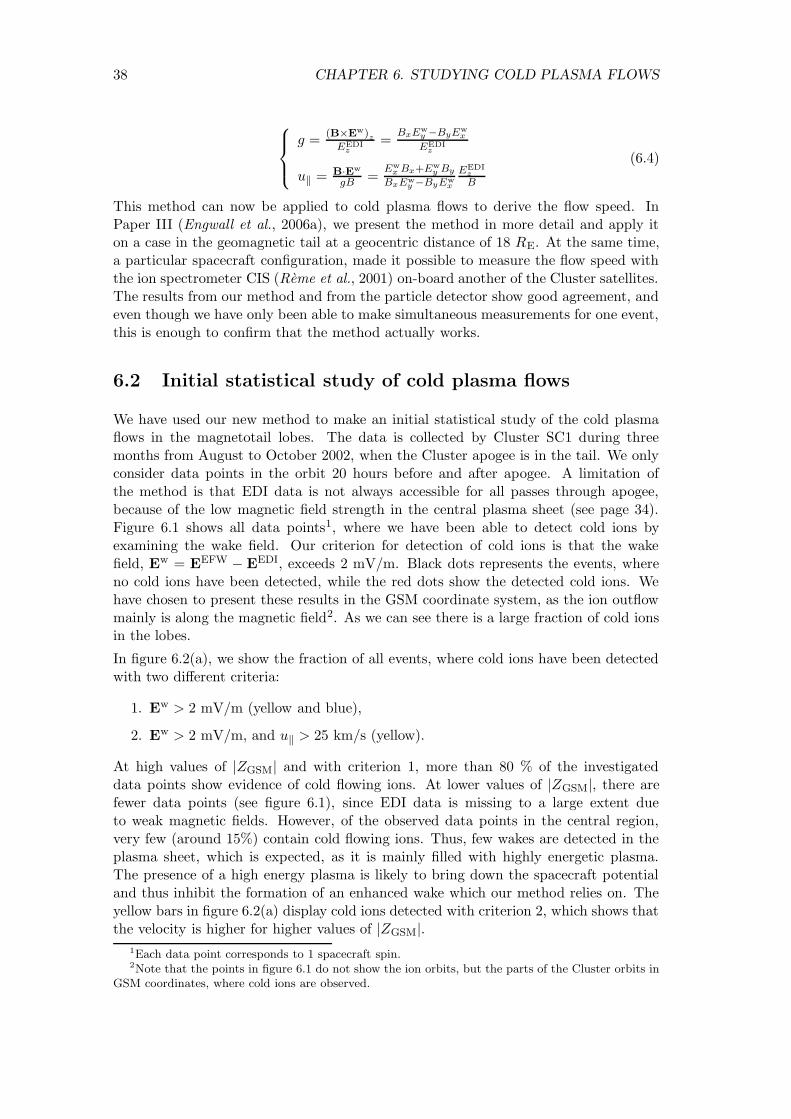
38 CHAPTER 6. STUDYING COLD PLASMA FLOWS

g =(B×E

w)z

EEDIz

=BxEw

y −ByEwx

EEDIz

u‖ = B·Ew

gB =Ew

x Bx+Ewy By

BxEwy −ByEw

x

EEDIz

B

(6.4)

This method can now be applied to cold plasma flows to derive the flow speed. InPaper III (Engwall et al., 2006a), we present the method in more detail and apply iton a case in the geomagnetic tail at a geocentric distance of 18 RE. At the same time,a particular spacecraft configuration, made it possible to measure the flow speed withthe ion spectrometer CIS (Reme et al., 2001) on-board another of the Cluster satellites.The results from our method and from the particle detector show good agreement, andeven though we have only been able to make simultaneous measurements for one event,this is enough to confirm that the method actually works.

6.2 Initial statistical study of cold plasma flows

We have used our new method to make an initial statistical study of the cold plasmaflows in the magnetotail lobes. The data is collected by Cluster SC1 during threemonths from August to October 2002, when the Cluster apogee is in the tail. We onlyconsider data points in the orbit 20 hours before and after apogee. A limitation ofthe method is that EDI data is not always accessible for all passes through apogee,because of the low magnetic field strength in the central plasma sheet (see page 34).Figure 6.1 shows all data points1, where we have been able to detect cold ions byexamining the wake field. Our criterion for detection of cold ions is that the wakefield, Ew = EEFW − EEDI, exceeds 2 mV/m. Black dots represents the events, whereno cold ions have been detected, while the red dots show the detected cold ions. Wehave chosen to present these results in the GSM coordinate system, as the ion outflowmainly is along the magnetic field2. As we can see there is a large fraction of cold ionsin the lobes.

In figure 6.2(a), we show the fraction of all events, where cold ions have been detectedwith two different criteria:

1. Ew > 2 mV/m (yellow and blue),

2. Ew > 2 mV/m, and u‖ > 25 km/s (yellow).

At high values of |ZGSM| and with criterion 1, more than 80 % of the investigateddata points show evidence of cold flowing ions. At lower values of |ZGSM|, there arefewer data points (see figure 6.1), since EDI data is missing to a large extent dueto weak magnetic fields. However, of the observed data points in the central region,very few (around 15%) contain cold flowing ions. Thus, few wakes are detected in theplasma sheet, which is expected, as it is mainly filled with highly energetic plasma.The presence of a high energy plasma is likely to bring down the spacecraft potentialand thus inhibit the formation of an enhanced wake which our method relies on. Theyellow bars in figure 6.2(a) display cold ions detected with criterion 2, which shows thatthe velocity is higher for higher values of |ZGSM|.

1Each data point corresponds to 1 spacecraft spin.2Note that the points in figure 6.1 do not show the ion orbits, but the parts of the Cluster orbits in

GSM coordinates, where cold ions are observed.

6.2. INITIAL STATISTICAL STUDY OF COLD PLASMA FLOWS 39

−20 −15 −10 −5 0−15

−10

−5

0

5

10

XGSE/GSM

[RE]

ZG

SM

[RE]

−10 −5 0 5 10−15

−10

−5

0

5

10

YGSM

[RE]

ZG

SM

[RE]

Earth

Figure 6.1: Detection of cold ions in the geomagnetic tail. Red dots show where cold ions havebeen detected with the method described in 6.1, while the black dots represent no detected ions. In amajority of the events, we detect cold ions.

In figure 6.2(b), we present the outward velocity distribution along the magnetic field.The mean speed is 29.4 km/s (red line) and the median speed is 21.8 km/s (green line).Figure 6.3(a) shows the corresponding outward flux of cold ions. The plasma densityis inferred from the spacecraft potential measured by EFW (see figure 4.1) (Pedersenet al., 2001)3. Both the outward speed and flux are close to the values from the polarwind survey with the Polar spacecraft reported by Su et al. (1998), even though ourvalues are somewhat lower. One explanation for the lower speed in our study is that Suet al. (1998) probably miss a large part of the low-energy ions, as discussed in section2.3.2.

The ionospheric mass loss of protons, M Isph

H+ , corresponding to the outward proton flux,FH+ , can be estimated as

M Isph

H+ = 2FH+Ao, (6.5)

where FH+ is the observed flux and Ao the equivalent polar cap area at the observationsite. The factor 2 accounts for the two polar caps. Ao is given from the conservationof magnetic flux, Ao = Apc

Bpc

Bo, where Apc is the area of one polar cap, Bpc and Bo are

3It should be noted that there is some uncertainty in the relation between the plasma density andthe spacecraft potential in tenuous plasmas, and the values of the outward flux should be taken asorder of magnitude estimates. In an extended study, a more accurate calibration of the plasma densityshould be included.

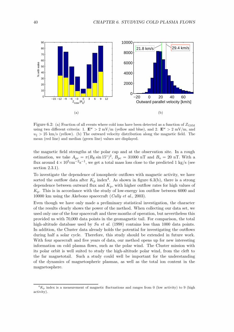
40 CHAPTER 6. STUDYING COLD PLASMA FLOWS

−15 −12 −9 −6 −3 0 3 6 9 120

10

20

30

40

50

60

70

80

90

ZGSM

[RE]

% w

ith w

ake

(a)

−20 0 20 40 600

2000

4000

6000

8000

10000

Outward parallel velocity [km/s]

29.4 km/s21.8 km/s

(b)

Figure 6.2: (a) Fraction of all events where cold ions have been detected as a function of ZGSM

using two different criteria: 1. Ew > 2 mV/m (yellow and blue), and 2. Ew > 2 mV/m, andu‖ > 25 km/s (yellow). (b) The outward velocity distribution along the magnetic field. Themean (red line) and median (green line) values are displayed.

the magnetic field strengths at the polar cap and at the observation site. In a roughestimation, we take Apc = π(RE sin 15◦)2, Bpc = 31000 nT and Bo = 20 nT. With aflux around 4× 105cm−2s−1, we get a total mass loss close to the predicted 1 kg/s (seesection 2.3.1).

To investigate the dependence of ionospheric outflows with magnetic activity, we havesorted the outflow data after Kp index4. As shown in figure 6.3(b), there is a strongdependence between outward flux and Kp, with higher outflow rates for high values ofKp. This is in accordance with the study of low-energy ion outflow between 6000 and10000 km using the Akebono spacecraft (Cully et al., 2003).

Even though we have only made a preliminary statistical investigation, the characterof the results clearly shows the power of the method. When collecting our data set, weused only one of the four spacecraft and three months of operation, but nevertheless thisprovided us with 70,000 data points in the geomagnetic tail. For comparison, the totalhigh-altitude database used by Su et al. (1998) contains less than 1000 data points.In addition, the Cluster data already holds the potential for investigating the outflowsduring half a solar cycle. Therefore, this study should be extended in future work.With four spacecraft and five years of data, our method opens up for new interestinginformation on cold plasma flows, such as the polar wind. The Cluster mission withits polar orbit is well suited to study the high-altitude polar wind, from the cleft tothe far magnetotail. Such a study could well be important for the understandingof the dynamics of magnetospheric plasmas, as well as the total ion content in themagnetosphere.

4Kp index is a measurement of magnetic fluctuations and ranges from 0 (low activity) to 9 (highactivity).

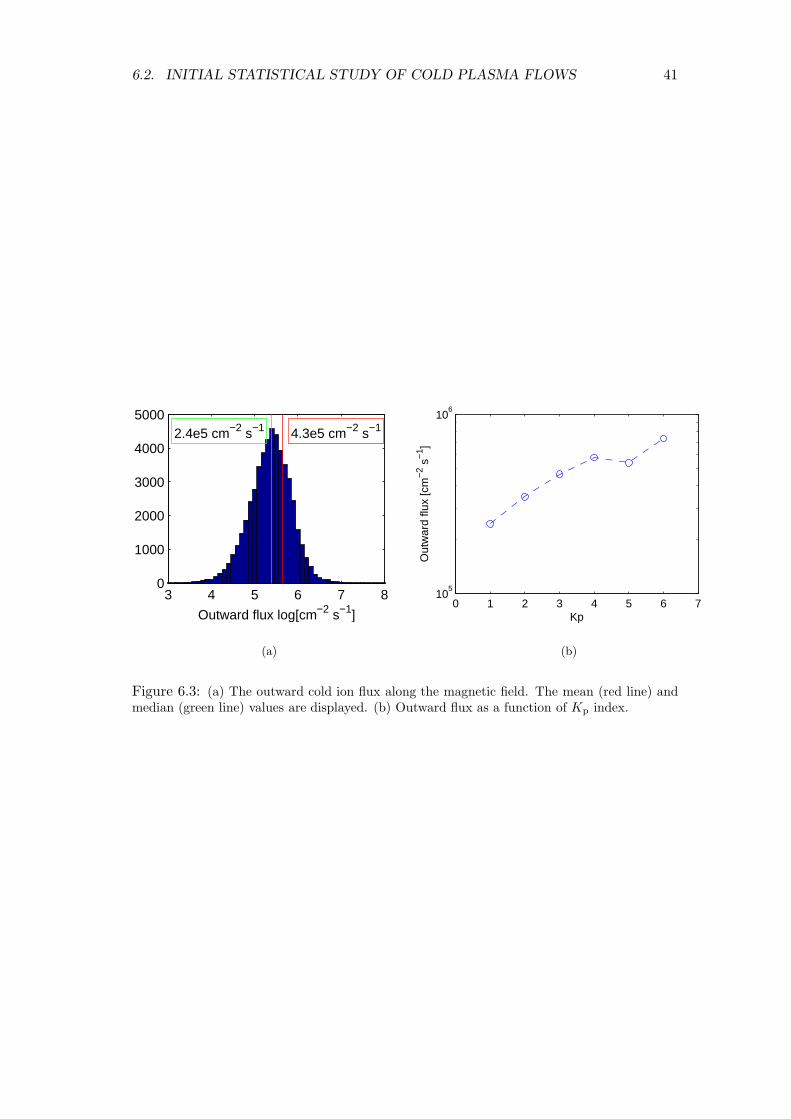
6.2. INITIAL STATISTICAL STUDY OF COLD PLASMA FLOWS 41

3 4 5 6 7 80

1000

2000

3000

4000

5000

Outward flux log[cm−2 s−1]

4.3e5 cm−2 s−12.4e5 cm−2 s−1

(a)

0 1 2 3 4 5 6 710

5

106

Kp

Out

war

d flu

x [c

m−

2 s−

1 ]

(b)

Figure 6.3: (a) The outward cold ion flux along the magnetic field. The mean (red line) andmedian (green line) values are displayed. (b) Outward flux as a function of Kp index.

Chapter 7

Summary of publications

7.1 Paper I: Wake formation behind positively charged

spacecraft in flowing tenuous plasmas

Authors: E. Engwall, A. I. Eriksson, and J. Forest

Journal: Physics of Plasmas

Status: In review

We report results from a study of enhanced wake formation behind positively chargedspacecraft in flowing tenuous plasmas using rough analytical estimates and numericalsimulations. For the numerical simulations we have used the code package PicUp3Drun on a common desktop PC.1 These simulations have provided new knowledge onthe size and shape of the wake, as well as scaling to different plasma parameters. Themost evident results are that (a) a low ion temperature causes a large ion wake, and(b) a high electron temperature leads to a more negative potential in the wake. Wehave modeled the spacecraft body and the spacecraft booms separately, which makesit possible to investigate which part creates the largest wake. Even for very thin wirebooms (thickness on the order of a few millimeters), the wake can grow very big, sincethe potential structure around the booms will increase the effective size of the obstacleto the plasma flow with three orders of magnitude. Around the spacecraft body thepotential decreases much more quickly. This was evident in the simulations, showinga much more negative wake potential behind the booms than behind the spacecraftbody.

Moreover, we have compared the simulation results to measurements from the Clusterdouble-probe instrument EFW, where we suspect influence from an enhanced wake(Eriksson et al., 2006a). We have seen that the magnitude of the suspected wake fielddetected by EFW is consistent with the simulation results. The wake spin signaturesof EFW have also been well reproduced by the simulations, further supporting the ideaof enhanced wake formation behind Cluster.

1The PIC method and the PicUp3D code are described in more detail in Engwall (2004).

42

CHAPTER 7. SUMMARY OF PUBLICATIONS 43

7.2 Paper II: Double-probe measurements in cold tenu-ous space plasma flows

Authors: E. Engwall and A. I. Eriksson

Journal: IEEE Trans. Plasma Sci.

Status: In review

In this paper we discuss the two main sources for spurious electric fields in double-probemeasurements in cold flowing tenuous space plasmas: 1. asymmetric photoemission be-tween probes and other electrical elements of the spacecraft, and 2. enhanced wakes.By performing a Fourier analysis of EFW spin data, we have found that the photoasym-metric field, Ea, can be represented by

Ea(θ) = E0a cos θ, (7.1)

where θ is the angle between the boom and the direction to the Sun. The photoasym-metric field is often referred to as apparent sunward field or sunward offset. In the caseof Cluster its amplitude is typically around 1 mV/m.

Furthermore, we assume that the wake field can be written as

Ew = aw1 cos θb + aw3 cos(3θb) + aw5 cos(5θb), (7.2)

where θb is the angle between the boom and the wake direction. Now, Fourier analysisof EFW spin data including wake effects makes it possible to determine the angle ofthe wake, as well as the Fourier coefficients aw1, aw3 and aw5. We have seen that theFourier coefficients are dependent on satellite potential: the signatures become moresinusoidal for higher satellite potentials, which is expected for an enhanced wake field.

7.3 Paper III: Low-energy (order 10 eV) ion flow in themagnetotail lobes inferred from spacecraft wake ob-

servations

Authors: E. Engwall, A. I. Eriksson, M. Andre, I. Dandouras, G. Paschmann, J. Quinn, andK. Torkar

Journal: Geophysical Research Letters

Status: Accepted

We present a case study of cold ions in the magnetotail lobes at 18 RE detected byCluster. The ions are so low in energy (order 10 eV) that they are not normallydetectable by ordinary particle instruments due to high positive spacecraft potentials(40-60 V). However, for this event, artificial spacecraft potential control reduces thespacecraft potential to around +7 V and the Cluster ion detector is in a special low-energy mode, making it possible to measure the cold ions. At the same time we are ableto detect and derive the flow velocity of the cold ions using electric field instruments.The method is based on the fact that an enhanced wake is formed behind a positivelycharged spacecraft in a flowing tenuous plasma as described in section 6.1.

44 CHAPTER 7. SUMMARY OF PUBLICATIONS

The flow measurements using both methods are in accordance with the polar windsurvey at 8 RE by Su et al. (1998), confirming the continuation of low-energy ionoutflows to at least 18 RE. The good agreement between the two methods shows that asimple model of the wake field in combination with electric field data from double-probeand electron drift instruments can be used to estimate the flow velocity of low-energy,supersonically flowing ions.

Acknowledgements

This work has been performed at the Department of Astronomy and Space Physics,Uppsala University, and at the Swedish Institute of Space Physics, Uppsala Division.First of all, I would like to thank my fantastic supervisor Anders I. Eriksson, who hasbeen a perfect teacher, collaborator and friend: skilled, enthusiastic and interested.Anders’s great devotion has been clear during the past six months: even though Ihave not been present at the institute, we have been able to discuss the papers andthis thesis during long telephone conversations in late evenings and at weekends. Myassistant supervisor Mats Andre, who has provided invaluable knowledge and broughtrealism into our plans, is also sincerely thanked.

The personnel at both the Department of Astronomy and Space Physics and at theSwedish Institute of Space Physics is acknowledged for creating a nice and friendlyworking environment. I would especially like to thank my fellow PhD students andMaster thesis students for fruitful discussions and fun social events. The members ofthe board of IRFU IF and the Swedish Institute of Space Physics are recognised formaking it possible (after some minor delay) to rent a hall and field for our weeklyfootball games, which I already miss a lot.

45

Bibliography

Abe, T., B. A. Whalen, A. W. Yau, R. E. Horita, S. Watanabe, and E. Sagawa, EXOS-D (Akebono) SMS observations of the polar wind, Journal of Geophysical Research,98, 11,191–11,203, 1993.

Abe, T., S. Watanabe, B. A. Whalen, A. W. Yau, and E. Sagawa, Observations ofpolar wind and thermal ion outflow by Akebono/SMS, Journal of Geomagnetismand Geoelectricity, 48, 319–325, 1996.

Axford, W. I., The polar wind and the terrestrial helium budget, Journal of GeophysicalResearch, 73, 6855–6859, 1968.

Banks, P. M., and T. E. Holzer, The polar wind, Journal of Geophysical Research,73 (21), 6846–6854, 1968.

Bauer, O. H., R. Grard, G. Haerendel, and A. Pedersen, Influence of wake and pho-toemission on electric field measurements with a double probe on GEOS-2, in Space-craft/Plasma Interactions and their Influence on Field and Particle Measurements,ESA SP-198, pp. 51–56, 1983.

Chappell, C. R., T. E. Moore, and J. H. Waite, The ionosphere as a fully adequatesource of plasma for the Earth’s magnetosphere, Journal of Geophysical Research,92 (11), 5896–5910, 1987.

Chappell, C. R., B. L. Giles, T. E. Moore, D. C. Delcourt, P. D. Craven, and M. O.Chandler, The adequacy of the ionospheric source in supplying magnetospheric plas-mas, Journal of Atmospheric and Solar-Terrestrial Physics, 62, 421–436, 2000.

Chen, F. F., Introduction to Plasma Physics and Controlled Fusion, 2nd ed., PlenumPress, New York, 1984.

Chen, S.-H., and T. E. Moore, Dayside flow bursts in the Earth’s outer magnetosphere,Journal of Geophysical Research, 109, doi: 10.1029/2003JA010007, 2004.

Cully, C. M., E. F. Donovan, A. W. Yau, and G. G. Arkos, Akebono/SuprathermalMass Spectrometer observations of low-energy ion outflow: Dependence on mag-netic activity and solar wind conditions, Journal of Geophysical Research, 108, doi:10.1029/2001JA009200, 2003.

Decreau, P. M. E., et al., Early results from the WHISPER instrument on Cluster: anoverview, Annales Geophysicae, 19, 1241–1258, 2001.

46

BIBLIOGRAPHY 47

Engwall, E., Numerical studies of spacecraft-plasma interaction: Simulations of wakeeffects on the Cluster electric field instruments EFW, IRF Scientific Report 284,Swedish Institute of Space Physics, http://www.irf.se/Publications/, 2004.

Engwall, E., and A. I. Eriksson, Double-probe measurements in cold flowing tenuousspace plasmas, IEEE Trans. Plasma Sci., in review, 2006.

Engwall, E., A. I. Eriksson, M. Andre, I. Dandouras, G. Paschmann, J. Quinn, andK. Torkar, Low-energy (order 10 ev) ion flow in the magnetotail inferred from space-craft wake observations, Geophysical Research Letters, accepted, 2006a.

Engwall, E., A. I. Eriksson, and J. Forest, Wake formation behind positively chargedspacecraft in flowing tenuous plasmas, Physics of Plasmas, in review, 2006b.

Eriksson, A., et al., Electric field measurements on Cluster: Comparing the double-probe and electron drift technique, Annales Geophysicae, in press, 2006a.

Eriksson, A. I., L. Wedin, J.-E. Wahlund, and B. Holback, Analysis of Freja chargingevents: Modelling of Freja observations by spacecraft charging codes, IRF ScientificReport 252, Swedish Institute of Space Physics, 1999.

Eriksson, A. I., et al., RPC-LAP: The Rosetta Langmuir probe instrument, Space Sci.Rev., in review, 2006b.

Escoubet, C. P., A. Pedersen, R. Schmidt, and P. A. Lindqvist, Density in the magne-tosphere inferred from ISEE 1 spacecraft potential, Journal of Geophysical Research,102, 17,595–17,609, 1997.

Escoubet, C. P., M. Fehringer, and M. Goldstein, The Cluster mission, Annales Geo-physicae, 19, 1197–1200, 2001.

Etcheto, J., and A. Saint-Marc, Anomalously high plasma densities in the plasma sheetboundary layer, Journal of Geophysical Research, 90, 5338–5344, 1985.

Fahleson, U., Theory of electric field measurements conducted in the magnetospherewith electric probes, Space Science Reviews, 7, 238–262, 1967.

Garrett, H. B., The charging of spacecraft surfaces, Reviews of Geophysics and SpacePhysics, 19 (4), 577–616, 1981.

Goldstein, H., C. Poole, and J. Safko, Classical Mechanics, 3rd ed., Addison Wesley,San Fransisco, 2002.

Gombosi, T. I., Physics of the Space Environment, Cambridge University Press, Cam-bridge, 1998.

Grard, R. J. L., Properties of the satellite photoelectron sheath derived from photoe-mission laboratory measurements, Journal of Geophysical Research, 78, 2885–2906,1973.

Gustafsson, G., et al., The Electric Field and Wave Experiment for the Cluster Mission,Space Science Reviews, 79, 137–156, 1997.

48 BIBLIOGRAPHY

Gustafsson, G., et al., First results of electric field and density observations by ClusterEFW based on initial months of operation, Annales Geophysicae, 19, 1219–1240,2001.

Hoffman, J. H., Studies of the composition of the ionosphere with a magnetic deflectionmass spectrometer, International journal of mass spectrometry and ion physics, 4,315–322, 1970.

Hoffman, J. H., and W. H. Dodson, Light ion concentrations and fluxes in the polarregions during magnetically quiet times, Journal of Geophysical Research, 85 (14),626–632, 1980.

Hoffman, J. H., W. H. Dodson, C. R. Lippincott, and H. D. Hammack, Initial ioncomposition results from the ISIS 2 satellite, Journal of Geophysical Research, 79 (18),4246–4251, 1974.

Kivelson, M. G., and C. T. Russel, Introduction to Space Physics, Cambridge UniversityPress, Cambridge, 1995.

Laakso, H., T. L. Aggson, and R. Pfaff Jr., Plasma gradient effects on double probemeasurements in the magnetosphere, Annales Geophysicae, 13, 130–146, 1995.

Lockwood, M., M. O. Chandler, J. L. Horwitz, J. H. Waite Jr., T. E. Moore, and C. R.Chappell, The cleft ion fountain, Journal of Geophysical Research, 90, 9736–9748,1985.

Matsui, H., T. Mukai, S. Ohtani, K. Hayashi, R. C. Elphic, M. F. Thomsen, andH. Matsumoto, Cold dense plasma in the outer magnetosphere, Journal of Geophys-ical Research, 104, 25,077–25,095, 1999.

Medicus, G., Theory of electron collection of spherical probes, Journal of AppliedPhysics, 32, 2512–2520, 1961.

Medicus, G., Spherical Langmuir probe in ”drifting” and ”accelerated” Maxwelliandistribution, Journal of Applied Physics, 33, 3094–3100, 1962.

Moore, T. E., et al., High-altitude observations of the polar wind, Science, 277, 349–351, 1997.

Moore, T. E., et al., Polar/TIDE results on polar ion outflows, in Sun-Earth PlasmaConnections, Geophysical Monograph 109, pp. 87–101, American Geophysical Union,1999.

Mott-Smith, H., and I. Langmuir, The theory of collectors in gaseous discharges, Phys-ical Review, 28, 727–763, 1926.

Mozer, F. S., Analyses of techniques for measuring DC and AC electric fields in themagnetosphere, Space Science Reviews, 14, 272–313, 1973.

Nagai, T., J. H. Waite, J. L. Green, C. R. Chappell, R. C. Olsen, and R. H. Comfort,First measurements of supersonic polar wind in the polar magnetosphere, GeophysicalResearch Letters, 11, 669–672, 1984.

BIBLIOGRAPHY 49

Orsini, S., M. Candidi, M. Stockholm, and H. Balsiger, Injection of ionospheric ionsinto the plasma sheet, Journal of Geophysical Research, 95, 7915–7928, 1990.

Parks, G. K., Physics of Space Plasmas, 2nd ed., Addison Wesley, Redwood City, 1991.

Paschmann, G., C. E. McLlwain, J. M. Quinn, R. B. Torbert, and E. C. Whipple, TheElectron Drift Technique for Measuring Electric and Magnetic Fields, in Measure-ment Techniques in Space Plasmas: Fields, Geophysical Monograph 103, pp. 29–38,American Geophysical Union, 1998.

Paschmann, G., et al., The Electron Drift Instrument on Cluster: overview of firstresults, Annales Geophysicae, 19, 1273–1288, 2001.

Pedersen, A., Solar wind and magnetosphere plasma diagnostics by spacecraft electro-static potential measurements, Annales Geophysicae, 13, 118–121, 1995.

Pedersen, A., C. A. Cattell, C.-G. Falthammar, V. Formisano, P.-A. Lindqvist,F. Mozer, and R. Torbert, Quasistatic electric field measurements with sphericaldouble probes on the GEOS and ISEE satellites, Space Science Reviews, 37, 269–312, 1984.

Pedersen, A., F. Mozer, and G. Gustafsson, Electric field measurements in a tenuousplasma with spherical double probes, in Measurement Techniques in Space Plasmas:Fields, Geophysical Monograph 103, pp. 1–12, American Geophysical Union, 1998.

Pedersen, A., P. Decreau, P. Escoubet, G. Gustafsson, H. Laakso, P.-A. Lindqvist,B. Lybekk, F. Mozer, and A. Vaivads, Four-point high time resolution informationon electron densities by the electric field experiments (EFW) on Cluster, AnnalesGeophysicae, 19, 1483–1489, 2001.

Reme, H., et al., First multispacecraft ion measurements in and near the Earth’s mag-netosphere with the identical Cluster ion spectrometry (CIS) experiment, AnnalesGeophysicae, 19, 1303–1354, 2001.

Sandahl, I., Norrsken - Budbarare fran rymden, Atlantis, Stockholm, 1998.

Sauvaud, J.-A., et al., Intermittent thermal plasma acceleration linked to sporadicmotions of the magnetopause, first Cluster results, Annales Geophysicae, 19, 1523–1532, 2001.

Sauvaud, J.-A., et al., Case studies of the dynamics of ionospheric ions in the Earth’smagnetotail, Journal of Geophysical Research, 109, doi: 10.1029/2003JA009996,2004.

Schunk, R. W., Ionospheric outflow, in Sun-Earth Plasma Connections, GeophysicalMonograph 109, pp. 195–206, American Geophysical Union, 1999.

Schunk, R. W., and J. J. Sojka, Global ionosphere-polar wind system during changingmagnetic activity, Journal of Geophysical Research, 102, 11,625–11,651, 1997.

Seki, K., R. C. Elphic, M. F. Thomsen, J. Bonnell, J. P. McFadden, E. J. Lund,M. Hirahara, T. Terasawa, and T. Mukai, A new perspective on plasma supplymechanisms to the magnetotail from a statistical comparison of dayside mirroringO+ at low altitudes with lobe/mantle beams, Journal of Geophysical Research (SpacePhysics), 107, 7–1, doi:10.1029/2001JA900122, 2002.

50 BIBLIOGRAPHY

Seki, K., et al., Cold ions in the hot plasma sheet of Earth’s magnetotail, Nature, 422,589–591, 2003.

Su, Y.-J., J. L. Horwitz, T. E. Moore, B. L. Giles, M. O. Chandler, P. D. Craven,M. Hirahara, and C. J. Pollock, Polar wind survey with the Thermal Ion DynamicsExperiment/Plasma Source Instrument suite aboard POLAR, Journal of GeophysicalResearch, 103, 29,305–29,337, 1998.

Torkar, K., et al., An experiment to study and control the Langmuir sheath aroundINTERBALL-2, Annales Geophysicae, 16, 1086–1096, 1998.

Torkar, K., et al., Active spacecraft potential control for Cluster - implementation andfirst results, Annales Geophysicae, 19, 1289–1302, 2001.

Wahlund, J.-E., et al., Cassini measurements of cold plasma in the ionosphere of Titan,Science, 308, 986–989, 2005.

Yau, A. W., and M. Andre, Sources of ion outflow in the high latitude ionosphere,Space Science Reviews, 80, 1–25, 1997.

Paper I

Wake formation behind positively charged spacecraft in flowing tenuous plasmas

E. EngwallDepartment of Astronomy and Space Physics, Uppsala University, Sweden and

Swedish Institute of Space Physics, Uppsala, Sweden

A. I. ErikssonSwedish Institute of Space Physics, Uppsala, Sweden

J. ForestSwedish Institute of Space Physics, Kiruna, Sweden and

Artenum Company, Paris, France

(Dated: March 10, 2006)

Spacecraft in tenuous plasmas become positively charged because of photoelectron emission. Ifthe plasma is supersonically drifting with respect to the spacecraft, a wake forms behind it. Whenthe kinetic energy of the positive ions in the plasma is not sufficient to overcome the electrostaticbarrier of the spacecraft potential, they scatter on the potential structure from the spacecraft ratherthan get absorbed or scattered by the spaceraft body. For tenuous plasmas with Debyelenghtsmuch exceeding the spacecraft size, the potential structure extends farfram the spacecraft, andconsequently the wake is in this case of transverse dimensions much larger than the spacecraft. Thisenhanced wake formation process is demonstrated by theoretical analysis and computer simulations.Comparison to observations from the Cluster satellites show good agreement.

I. INTRODUCTION

When a spacecraft moves through a plasma at a rela-tive speed exceeding the ion thermal speed in the plasma,a wake will form behind it. Since in the space plasmaswhere this happens usually Ti ∼ Te, so that the space-craft also moves faster than ion acoustic waves, we referto this motion as supersonic. Motion supersonic with re-spect to electrons as well as ions is rare: the typical caseis the mesosonic flow, where the spacecraft is supersonicwith respect to the ions but subsonic with respect to theelectrons. The wake thus becomes negatively charged,due to the thermal motion of the electrons.

Mesosonic spacecraft motion, and hence the occurrenceof a negatively charged wake behind the spacecraft, isvery common. The prime examples are the ionosphereand solar wind. In the ionosphere, typical spacecraftmove at speeds around 7 km/s in a plasma with ionthermal speed on the order of 4 km/s for protons and0.25 km/s for oxygen. In the solar wind, a flow speed of400 km/s and proton thermal speed of 40 km/s are typ-ical values. Less obvious regions of mesosonic spacecraftmotion are the polar cap and tail lobes of the Earth’smagnetosphere. These regions are sometimes thought ofas essentially void of plasma, but are often filled witha very tenuous (∼ 0.1 cm−3) but mesosonic cold plasmaoutflow from the ionosphere, driven by e.g. the polar windor cleft ion fountain1–3. Electric field measurements onthe Cluster satellites have shown regular occurrence ofwakes in these regions4.

The three regions mentioned presents three differentregimes for wake formation. In the ionosphere, the space-craft potential with respect to the surrounding plasma,Vsc, usually is negative and a few times the electron tem-perature Te in magnitude, due to the higher mobility of

electrons. This case has been studied for a long time,and a substantial literature has built up over the years.An old, but still very useful summary was provided byAl’pert et al.5, with a review of later work given by Hast-ings6. One of the results is that the negative potentialstructure, from the spacecraft itself as well as from thenegatively charged wake, focuses ions into the wake, en-hancing the filling-in of the wake.

The solar wind is much more tenuous than the iono-sphere (typically 5 cm−3), implying that the electronsrandomly collected by the spacecraft gives a currentmuch smaller than the photoemission current from thesunlit spacecraft. The result is positive values of Vsc,typically on the order of 5 - 10 V. This is so much lowerthan the ion flow kinetic energy of typically 1 keV (pro-tons) that the charge of the spacecraft is quite irrelevantfor the wake formation, and the elongated wake formingbehind the spacecraft has its width determined by thespacecraft dimensions [see Figure 1(a)]. Much existingwork on theory and simulation of wake formation be-hind ionospheric spacecraft is relevant for this situationas well.

The case of tenuous mesosonic plasma flows in the ter-restrial magnetosphere is quite different. In the verytenuous plasmas of the polar cap and tail lobe regions(∼ 0.1 cm−3 or less), the spacecraft potential often goesabove 20 V positive, sometimes as high as 50 V or more7.Ion flow energies often stay at much lower values, around10 eV, with temperatures of a few eV3. In this case, i.e.when

KTi <miu

2

2< eVsc, (1)

the ions will scatter on the repulsive potential distribu-tion from the spacecraft. The wake size transverse to the

2

i i i scmv /2 > KT , mv /2 > eV2 2

KT < mv /2 < eVi i sc2 2

+ − Narrow wake

−

−−

−

+−

Enhanced wake

(b)

(a)

FIG. 1: Sketch of wake formation in mesosonic flows. (a)For ion flow energies higher than the spacecraft potential,Vsc, the wake has the typical transverse size of the spacecraft(narrow wake case). (b) For ion flow energy below Vsc, ionswill scatter off the positive electrostatic potential from thespacecraft, creating an enhanced wake.

flow can thus be substantially larger than the spacecraftbody itself [see Figure 1(b)]. We call such a wake anenhanced wake.

In contrast to the large literature on wakes behind neg-atively charged spacecraft, relevant to the ionosphere,very few studies address wake formation behind posi-tive spacecraft, and only one of them concerns the casedescribed by relation 1. The very earliest theoreticalstudies on spacecraft wake formation treated the caseof a wake behind a point charge8 or line charge9 in amesosonic plasma flow in a formalism appliccable alsofor positive charges. As the obstacles in these cases areinfinitesimally small, while the calculated wake has a De-bye scale width, these studies catch an important featureof the enhanced wake discussed above. However, theassumption of small potentials, |Vsc| � miu

2/2, meansthat they cannot be directly used for quantitative studyof wakes in the situation described by relation 1. Thesame limitation applied to the laboratory study of wakesbehind thin cylinders by Hester and Sonin10, which in-cluded an experiment with positive cylinder potentials,eVsc ≈ 3 KTe ≈ 300 KTi ≈ miu

2/20. Despite the lowpotential of the obstacle, they detected an ion void sig-nificantly larger than the geometrical size of the obstacle.The elements of an enhanced wake, still in the small po-tential limit, can also be seen in the results of a simula-tion of a spherical Langmuir probe in a flowing plasma bySingh and Chagani11. The only studies of the case 1 thatwe are aware of are the simulations of spacecraft in thepolar wind flow by Zinin et al.12 and in a cometary comaby Roussel and Berthelier 13. However, in both cases theplasma has a Debye length much below the spacecraftsize, which means that the wake is not significantly en-

hanced by the electrostatic field around the spacecraft.In spacecraft applications, the possibility of enhanced

wakes was suggested by Bauer et al.14 and Pedersenet al.15 to explain particular features of electric fielddata from the ISEE (International Sun-Earth Explorer)and GEOS (GEOstationary Scientific Satellite) satellites.More recently, Eriksson et al.4 established the presenceof enhanced wakes in electric field data from the Clustersatellites. In parallel, we have done the numerical simu-lations presented in the present paper, using the Clusterdata for comparison and verification.

Following this introduction, we discuss enhanced wakeformation in Section 2, and the results from the com-puter simulations are presented in Section 3. In Section4 we compare the results from theory and simulations toCluster data in which the wake is detected.

II. ENHANCED WAKE FORMATION

The condition for enhanced wake formation (see Equa-tion 1) ensures that the size of the wake will not be de-termined directly by the spacecraft’s physical structure,but by the equipotential surface, where Φ ≈ miu

2/(2e),which few ions can overcome. If we assume vacuumconditions, the characteristic transverse dimension of aspherical spacecraft of radius r at 20 V in a plasma witha flow energy of 5 V will increase from πr2 to 16πr2,because the 5 V equipotential is at a distance of 4 rfrom the center of the spacecraft. This 16-fold increasein obstacle area may seem dramatic, but even more sois the effect on long booms, with which many spacecraftare equipped mainly for measurements of electric fields.Assuming these booms behave like infinite cylinders ofradius a in vacuum, except that the potential goes to ex-actly zero at a distance of gλD, where g > 1 is a realnumber, the potential field at a radial distance r from awire boom at potential V is:

Φ(r) = Vln(r) − ln(gλD)

ln(a) − ln(gλD). (2)

From this, we can obtain the radial distance rb at whichΦ(rb) = bV , where 0 < b < 1, as

rb = ab(gλD)(1−b). (3)

As an example, let us consider the Cluster wire boomswith 88 m tip-to-tip separation and a = 1.1 mm, a Debyelength of 15 m, and an arbitrary but reasonable choiceof g = 2. This gives r = 2.3 m for the 5 V equipotentialaround a wire boom at 20 V. The effective size of thebooms at right angles to the flow therefore increases from2.2 mm to 4.6 m, i.e. by three orders of magnitude. Thisincrease depends to some extent on the choice of g, butthe effect is certainly significant for all realistic valuesof g. It is therefore possible that long antennas, which

3

normally are negligible due to their small thickness, canbecome significant obstacles to the plasma flow in theconditions described by Equation (1).

How large can the potentials be in the cold, tenuousplasma wake behind the booms? Considering a wake ofslab-like geometry with thickness d � λD, we may as-sume perfect exclusion of ions and no effect on the elec-trons. Solving Poisson’s equation gives a maximum po-tential in such a wake of Φwake = (d/λD)2KTe/e. For awake of thickness d ∼ λD or larger, the potential satu-rates at Φwake ∼ KTe/e, as further accumulation of elec-trons is inhibited at larger potentials. The small wakearising behind the booms, for which d is on the order ofmillimeters, in for example the solar wind (λD ∼ 1 m),thus cannot give rise to appreciable potentials. How-ever, significant wake charging will arise in the case of

KTi < miu2

2< eVsc. This wake field may significantly

affect the measurements made by a double-probe instru-ment, as will be discussed in Section IV. To provide amore reliable basis for estimates regarding wake forma-tion behind booms and its size, we must turn to simula-tions. Simulations also provide information on the moregeometrically complex wake structure behind the space-craft body itself.

III. SIMULATIONS OF THE ENHANCED

WAKE FORMATION

A. Code and modeling

For modeling of the wake effect behind positivelycharged spacecraft, we used the open source simulationJAVA-based code package PicUp3D19, which implementsthe Particle-In-Cell method (PIC)20 to solve electrostaticspacecraft–plasma interaction problems. PicUp3D is de-signed for desktop PCs and was run on a dual-processorcomputer (2 × 2.40 GHz) with 2 GB RAM. A numberof simulations were carried out to examine the wake for-mation. Results are presented for simulations with twodifferent spacecraft geometries. In the first simulationswe modeled only the spacecraft body, while in the othersimulations we investigated the effects of long booms,neglecting the effects of the spacecraft body. We usedthe dimensions of the Cluster spacecraft in our simula-tions. They are cylindrical with a radius of 1.45 m anda height of 1.5 m. The distance between the boom tipsis 88 m. Both the spacecraft surface and a large part ofthe booms are conductive, so that they are at the samepotential (henceforth denoted spacecraft potential, Vsc).The last 3 m of the booms closest to the probes consistsof different electrical elements at potentials closer to theplasma potential, in order to make the electric field mea-surements more accurate21.

The input parameters for the simulations are chosento be consistent with high altitude polar wind conditionsderived from the POLAR satellite data presented by Suet al.3 as well as with Cluster observations in the polar

wind22. Table I gives the implemented simulation param-eters. With these plasma parameters the Debye length isin the range λD ≈ 12−24 m and the electron plasma fre-quency ωpe/2π ≈ 4−6 kHz. The ion flow defines the pos-itive y-direction. The integration time steps of all simu-lations were chosen in such a way that vmax∆t < 0.25∆r,where vmax is the maximal velocity of any particle, and∆r and ∆t the spatial and temporal step sizes, respec-tively. This ensures that no particle can cross a cell inless than a few time steps. The presented results are av-eraged over 30 ω−1

pe when the solution has reached steadystate in order to reduce statistical noise. To speed upthe simulations we used a mass ratio of mi/me = 100,while the ion kinetic energy remains unchanged. As willbe shown in section 3.4, this does not change the wakestructure close to spacecraft, but only the filling-in of ionsfarther downstream.

Plasma density, n0 [cm−3] 0.2, 0.4

Electron temperature, KTe [eV] 1.0, 2.0

Ion temperature, KTi [eV] 1.0, 2.0

Ion drift kinetic energy, miu2/2 [eV] 10

Spacecraft potential, Vsc [V] 20, 35

Magnetic field, B [nT] 0

TABLE I: Simulation parameters.

The magnetic field in magnetospheric regions withcold, tenuous plasmas is normally very low (typically 100nT) and was neglected in the simulations. This can bejustified by the very large Larmor radii (several km) forthe two dominant ion species in the polar wind (H+ andO+). The electron Larmor radius of a few tens of me-ters is closer to the scale of the problem. Assuming theelectrons to be unmagnetized may lead to overestimationof the electron densities in the wake. Since the flow ofelectrons is subsonic, this problem should, however, besmall.

For simplicity, in none of the cases were photoelec-trons included in the simulations. This approximationcan be justified by the high potential of the spacecraft(20 − 35 V), which means that it will recollect most ofthe emitted photoelectrons, whose typical energies are afew eV23. The photoelectrons will thus never build upany appreciable space charge around the spacecraft, andtherefore the vacuum potential is a very good approxi-mation.

PicUp3D uses a rectangular grid and Dirichlet bound-ary conditions, which have a great advantage in theireasy implementation, but special care must be taken toensure that the final results are not influenced substan-tially. The Dirichlet boundary conditions on the walls ofthe computational box (Φb = 0) can affect the deriva-tion of the potential in the rest of the box, if the wallsof the box are too close to the spacecraft. Theoretically,the walls should not be closer to the spacecraft than afew λD, in order to allow the Debye shielding to decreasethe potential to a satisfactorily low level. This assump-

4

tion was verified numerically for different sizes of com-putational boxes. On the inner boundary, i.e. at thespacecraft border, the potential is set as an input param-eter, and is not calculated self-consistently. The fixedspacecraft potential is of no concern in our case, as thespacecraft potential is related to the plasma density. ForCluster, Pedersen et al.7 extracted a density–potential re-lation from data. We can thus choose a potential whichis consistent with this relation. The rectangular grid canbe problematic, since the grid size should be sufficientlysmall in order to reflect the details of the spacecraft–plasma interactions. On the other hand, the computa-tional box has to be sufficiently large due to the impacton the potential distribution of the Dirichlet boundaryconditions. For a detailed description, a large number ofcomputational cells are therefore needed, which leads tolong computational times. Thus, the grid size is a com-promise between the requirement for a detailed descrip-tion and reasonable computational times. To be able toresolve finer structures of the booms we implemented ananalytical approximation, namely the effective potential,which is discussed in Section III C

B. Spacecraft body simulations

To obtain an idea of the wake formation behind thespacecraft body, we ran six reference simulations withdifferent polar wind parameters (see Table II). The driftenergy of the ions was 10 eV for all simulations, whichis well below the values of the spacecraft potential inTable II. To ensure small effects of the boundary condi-tions on the final results, the size of the computationalbox was chosen such that its walls were at least 3 λD

from the satellite and 1 λD from the points where thebooms would end if they were included. (The reason forconsidering the booms, althought they are not includedin these calculations, was that we wanted to see the sig-nature that would be obtained in a double-probe electricfield instrument, which uses such wire booms.) In thedownstream direction the wall was placed at least 10 λD

away from the satellite to avoid effects of the boundarieson the wake at large distances from the spacecraft.

In all simulations the grid size was 2.7×2.7×1.35 m3,resulting in different numbers of computational cells fordifferent Debye lengths. The spacecraft was modeledas a rectangular box with the same dimensions as thegrid, which approximates the cylindrical Cluster space-craft with a diameter of 2.9 m and height of 1.5 m fairlywell. In general, the average number of particles per cellis 8, which gives a reasonable accuracy. For the firstsimulation the number of particles was increased to 100particles per cell to investigate the effects of particle num-ber on numerical noise. The overall picture remainedthe same, while the detailed structure of the wake wassmoother due to better statistics. Since the computa-tional time increases with increasing number of macro-particles, while the noise is proportional to 1/

√Nmacro

24,

it is costly to reduce the noise. For our purposes, 8 par-ticles per cell gives sufficient accuracy.

Figure 2 shows results from Simulation 1 in Table II.As expected, there is a clearly visible wake in the iondensity behind the spacecraft. The dominating poten-tial structure is the decaying potential around the space-craft, giving essentially spherical equipotentials down to1 V. Behind the spacecraft a negatively charged wake isformed, reaching a minimum potential of -0.34 V.

−0.3−0.1

−0.02

0.1

13

Grid point in y−direction

Grid

poi

nt in

x−

dire

ctio

n

0 20 40 60 80 1000

10

20

30

40

50

FIG. 2: Averaged normalized density of ions and potentialbetween 20 ω−1

pe and 50 ω−1pe . The dashed circles show the

location of the Cluster EFW probes throughout a spin period.(The grid spacing is 2.7 m.) (a) Ion density in the x−y-planethrough the spacecraft. (The white square shows the locationof the spacecraft.) (b) Potential in the x−y-plane through thespacecraft (Vsc = 35 V). The minimum value of the potentialin the wake is −0.34 V. Equipotential contours are given at−0.3, −0.1, −0.01, 0.1, 1, 3, 10 and 35 V.

The results from all six simulations are shown in Ta-ble II, where characteristics of the wake, such as depth (involts), length, width, and height (in meters), are given.We defined two different criteria to determine the bordersof the wake, using the potential (Φ) and the ion density(ni). For the ion density, the surface where the ion den-sity has decreased to 75 % of its background density wasused, whereas for the potential we used the equipotentialof -0.1 V.

It can clearly be seen that the size of the wake de-creases with increasing ion temperature and decreasingelectron temperature, which is as expected. A high iontemperature allows the ions to diffuse behind the space-craft more quickly. Low electron temperatures result in asmaller potential in the wake. Moreover, at low electron

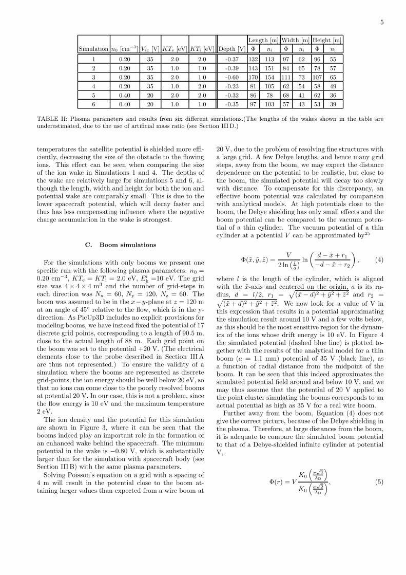
5

Length [m] Width [m] Height [m]

Simulation n0 [cm−3] Vsc [V] KTe [eV] KTi [eV] Depth [V] Φ ni Φ ni Φ ni

1 0.20 35 2.0 2.0 -0.37 132 113 97 62 96 55

2 0.20 35 1.0 1.0 -0.39 143 151 84 65 78 57

3 0.20 35 2.0 1.0 -0.60 170 154 111 73 107 65

4 0.20 35 1.0 2.0 -0.23 81 105 62 54 58 49

5 0.40 20 2.0 2.0 -0.32 86 78 68 41 62 36

6 0.40 20 1.0 1.0 -0.35 97 103 57 43 53 39

TABLE II: Plasma parameters and results from six different simulations.(The lengths of the wakes shown in the table areunderestimated, due to the use of artificial mass ratio (see Section III D.)

temperatures the satellite potential is shielded more effi-ciently, decreasing the size of the obstacle to the flowingions. This effect can be seen when comparing the sizeof the ion wake in Simulations 1 and 4. The depths ofthe wake are relatively large for simulations 5 and 6, al-though the length, width and height for both the ion andpotential wake are comparably small. This is due to thelower spacecraft potential, which will decay faster andthus has less compensating influence where the negativecharge accumulation in the wake is strongest.

C. Boom simulations

For the simulations with only booms we present onespecific run with the following plasma parameters: n0 =0.20 cm−3, KTe = KTi = 2.0 eV, Ei

k =10 eV. The gridsize was 4 × 4 × 4 m3 and the number of grid-steps ineach direction was Nx = 60, Ny = 120, Nz = 60. Theboom was assumed to be in the x−y-plane at z = 120 mat an angle of 45◦ relative to the flow, which is in the y-direction. As PicUp3D includes no explicit provisions formodeling booms, we have instead fixed the potential of 17discrete grid points, corresponding to a length of 90.5 m,close to the actual length of 88 m. Each grid point onthe boom was set to the potential +20 V. (The electricalelements close to the probe described in Section III Aare thus not represented.) To ensure the validity of asimulation where the booms are represented as discretegrid-points, the ion energy should be well below 20 eV, sothat no ions can come close to the poorly resolved boomsat potential 20 V. In our case, this is not a problem, sincethe flow energy is 10 eV and the maximum temperature2 eV.

The ion density and the potential for this simulationare shown in Figure 3, where it can be seen that thebooms indeed play an important role in the formation ofan enhanced wake behind the spacecraft. The minimumpotential in the wake is −0.80 V, which is substantiallylarger than for the simulation with spacecraft body (seeSection III B) with the same plasma parameters.

Solving Poisson’s equation on a grid with a spacing of4 m will result in the potential close to the boom at-taining larger values than expected from a wire boom at

20 V, due to the problem of resolving fine structures witha large grid. A few Debye lengths, and hence many gridsteps, away from the boom, we may expect the distancedependence on the potential to be realistic, but close tothe boom, the simulated potential will decay too slowlywith distance. To compensate for this discrepancy, aneffective boom potential was calculated by comparisonwith analytical models. At high potentials close to theboom, the Debye shielding has only small effects and theboom potential can be compared to the vacuum poten-tial of a thin cylinder. The vacuum potential of a thincylinder at a potential V can be approximated by25

Φ(x, y, z) =V

2 ln(

l

a

) ln

(

d − x + r1

−d − x + r2

)

, (4)

where l is the length of the cylinder, which is alignedwith the x-axis and centered on the origin, a is its ra-dius, d = l/2, r1 =

√

(x − d)2 + y2 + z2 and r2 =√

(x + d)2 + y2 + z2. We now look for a value of V inthis expression that results in a potential approximatingthe simulation result around 10 V and a few volts below,as this should be the most sensitive region for the dynam-ics of the ions whose drift energy is 10 eV. In Figure 4the simulated potential (dashed blue line) is plotted to-gether with the results of the analytical model for a thinboom (a = 1.1 mm) potential of 35 V (black line), asa function of radial distance from the midpoint of theboom. It can be seen that this indeed approximates thesimulated potential field around and below 10 V, and wemay thus assume that the potential of 20 V applied tothe point cluster simulating the booms corresponds to anactual potential as high as 35 V for a real wire boom.

Further away from the boom, Equation (4) does notgive the correct picture, because of the Debye shielding inthe plasma. Therefore, at large distances from the boom,it is adequate to compare the simulated boom potentialto that of a Debye-shielded infinite cylinder at potentialV,

Φ(r) = VK0

(

r

√2

λD

)

K0

(

a

√2

λD

) , (5)

6

−0.7−0.5

−0.3−0.1

−0.010.1

13


Grid

poi

nt in

x−

dire

ctio

n

0 20 40 60 80 100 1200

10

20

30

40

50

60

FIG. 3: Averaged results from the boom simulation between30 ω−1

pe and 60 ω−1pe . (The grid spacing is 4 m.) (a) Ion density

in the x − y-plane through the boom. (b) Ion density in they−z-plane through the boom. (c) Potential in the x−y-planecutting the boom. The minimum value of the potential in thewake is −0.80 V. Equipotential contours are given at −0.7,−0.5, −0.3, −0.1, −0.01, 0.1, 1, 5, and 10 V.

where K0 is a modified Bessel function of the second kind.The Debye-shielded potential is plotted in Figure 4 in redwith a = 1.1 mm and V = 35 V. As expected, the simu-lated potential and the shielded cylinder approach eachother far from the boom. Closer to the boom, the Debyeshielding expression (5) breaks down due to violation ofthe assumption eΦ � KTe inherent in the linear Debyeshielding law. The influence of the wake on the potentialcan clearly be seen in the difference in the upstream anddownstream directions in the simulation data.

To verify the validity of the effective potential we usedtwo simulations with the spacecraft body for the sameplasma parameters but different dimensions (4×4×4 m3

−80 −60 −40 −20 0 20 40 60 80

0

5

10

15

20

25

30

35

Radial distance from the midpoint of the boom [m]

Pot

entia

l (V

)

Results from simulationsHallen modelDebye shielded cylinder

FIG. 4: Comparison between the potential obtained from thesimulation (dashed blue line) and analytical models. The redline corresponds to an infinite Debye-shielded cylinder and theblack line to the model presented by Hallen25. The horizontalaxis gives the radial distance from the center of the boom inthe boom-flow plane [r in Figure 7(b)].

and 2.7 × 2.7 × 1.35 m3). In the first simulation thespacecraft is at 20 V. Using the concept of effective po-tential, we can expect this to correspond to a potential of3

√

4 × 4 × 4/(2.7× 2.7× 1.35)× 20V ≈ 37 V for a space-craft with dimensions 2.7× 2.7× 1.35 m3, assuming scal-ing of the potential as 1/r. In the second simulation thespacecraft potential was set to 35 V. The two simula-tions give essentially the same potential pattern from afew meters outside the spacecraft, which confirms thatthe use of effective potentials is acceptable.

D. Accuracy of the simulations

Before comparing the simulation results to spacecraftdata, the accuracy of the simulations should be discussed.In terms of basic modelling, two potentially importantfactors not included in the simulations are the magneti-zation of electrons (see Section III A) and the emissionand exchange of photoelectrons by different electrical ele-ments on the spacecraft. It is, for example, possible thatthe wake is filled to a large extent by photoelectrons emit-ted from the probes (as noted in Section III A photoelec-trons from the spacecraft can never contribute much tothe electron density due to the high spacecraft potential),rather than by natural plasma electrons. However, thephotoelectron temperature is on the order of a few eV,close to the temperature of the ambient plasma electrons.Therefore, the charge in a wake filled with photoelectronsshould not be very different from the resulting charge inthe simulations.

Numerical problems that might influence the final re-sults are the unphysical mass ratio, the Dirichlet bound-ary conditions and the modelling of the wire booms asdiscrete grid points.

7

1. Mass ratio

Using an artificial mass ratio between ions and elec-trons in the PIC simulations, will not significantly in-fluence the wake close to the spacecraft, since the wakepotential is small relative to the spacecraft potential dis-tribution. The orbit of a charged particle in any centralfield is determined completely by its kinetic energy percharge26, in analogy with how the Keppler motion in acentral gravitational field depends only on kinetic energyper mass, i.e. velocity squared. Deflection in such a po-tential is therefore accurately represented in a simulationwhere the kinetic energy is correctly represented, irre-spective of the mass actually used. The potential aroundthe spacecraft body can be well approximated as radiallysymmetric. For the potential around the finite booms,there is no perfect plane of symmetry, but at least forDebye lengths well below the boom length should radialsymmetry be a good approximation in the central partof the boom.

We therefore expect the artificial mass ratio to have im-pact mainly on the filling-in of the wake at large distancesfrom the spacecraft, where the space charge in the wakewill dominate the potential, and only if the potentialreaches values on the order of the ion temperature. Theeffect of the mass ratio has been examined by performingsimulations 1 to 4 for the spacecraft body with both real(mi/me = 1836) and (mi/me = 100) mass ratios. Thelength of the wake is in average 45% longer for the realmass ratio. However, as expected, the wake structureclose to the spacecraft is only marginally affected. Thisis evident when we examine the simulated signature of adouble-probe instrument (see Section IV B). The depen-dence of wake length on mass ratio implies that, for equalflow energies, a wake in an oxygen-dominated plasma willbe longer than in a hydrogen-dominated plasma. How-ever, we should also note that at the same flow velocityoxygen ions are 16 times as energetic as protons, mean-ing that relation 1 often is not satisfied and thus do notcontribute to the wake formation. In the high-altitudepolar wind, where many enhanced wakes are observed,the plasma is dominated by protons3.

2. Dirichlet conditions

The Dirichlet conditions of the PicUp3D code at theboundaries of the computational box (see Section III A)affect the potential close to the boundaries. In the pre-sented simulations, the box was chosen to be sufficientlylarge to achieve a good overall picture. The potentialdeep inside the wake is then only marginally affected. Ascan be seen in Figures 2(b) and 3(a), the ion density isnot significantly influenced by the Dirichlet conditions,due to the ion energy being high compared to the wakepotentials. In a sense the ions just scatter off the vac-uum field of the spacecraft or booms. To verify that theDirichlet conditions do not constitute a significant er-

ror source, we have performed test simulations with 50%larger computational boxes showing that only the poten-tial structures close to the boundaries are affected in thepresented simulations.

3. Wire booms

Numerical modeling of 88 m wire booms with a ra-dius of a few millimeters is a computational challenge.We have modeled the booms as a cluster of discrete gridpoints and compared the potential around the boom toresults from analytical models to be able to estimate aneffective potential for the boom. As described in the pre-vious section, the validity of this effective potential wasconfirmed for the spacecraft body. For the booms, themethod could be verified by comparison to adaptive-gridcodes.

IV. COMPARISON TO DATA FROM THE

CLUSTER SPACECRAFT

A. Cluster data

The Cluster mission is designed for four-point mea-surements in key regions of the terrestrial magneto-sphere and its adjacent environment in the solar wind,in particular boundary layers such as the bow shock andthe magnetopause27. Thanks to their polar orbits withperigee at 4 RE and apogee at 19.6 RE, the Clustersatellites sample a broad range of plasma regions, fromthe cold, dense plasmasphere to the hot, tenuous plasmasheet. The four spacecraft were designed with identicalpayloads, each carrying complete instrumentation for thestudy of particles and fields. For electric field measure-ments, Cluster includes two instruments using differenttechniques. The Electric Fields and Waves instrument(EFW) employs the well-known technique of measuringthe voltage between spherical electrostatic probes at theends of wire booms in the spacecraft spin plane21. Thetechnique allows sampling at essentially unlimited fre-quencies, and can operate under widely varying plasmaconditions, although great care is needed in the instru-ment design in order to minimize electrostatic distur-bances from the spacecraft and the probe supports. EFWhas two pairs of spherical probes (8 cm in diameter) sep-arated by 88 m wire booms (2.2 mm diameter). In addi-tion to the electric field, EFW provides a measurementof the spacecraft potential with respect to the ambientplasma, Vsc. The spin frequency of the satellites is 4 s.

The Electron Drift Instrument (EDI) uses a completelydifferent technique28, relying on observing the E × B

drift of electron beams emitted from the spacecraft andreturned by the ambient magnetic field, which thus hasto be sufficiently strong for the method to work. Usingelectrons in the keV range, this technique is quite immune

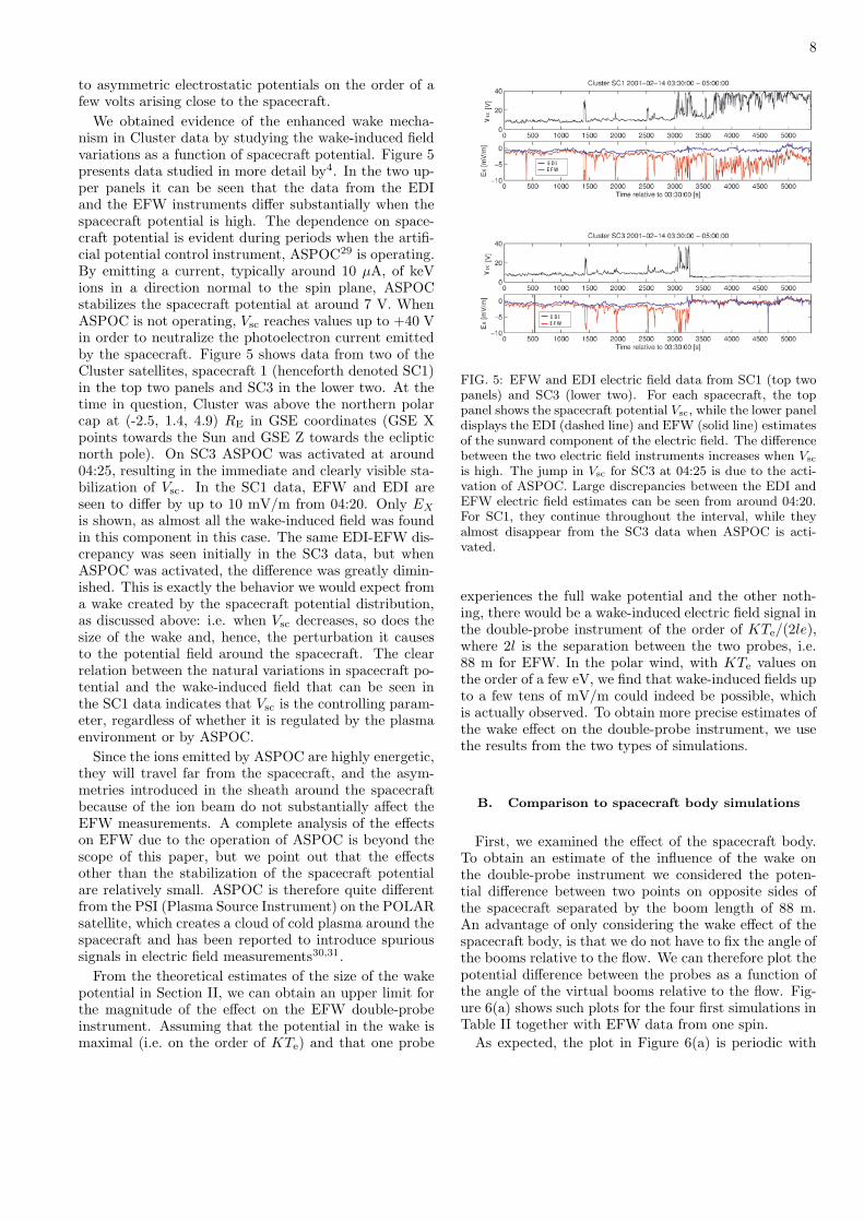
8

to asymmetric electrostatic potentials on the order of afew volts arising close to the spacecraft.

We obtained evidence of the enhanced wake mecha-nism in Cluster data by studying the wake-induced fieldvariations as a function of spacecraft potential. Figure 5presents data studied in more detail by4. In the two up-per panels it can be seen that the data from the EDIand the EFW instruments differ substantially when thespacecraft potential is high. The dependence on space-craft potential is evident during periods when the artifi-cial potential control instrument, ASPOC29 is operating.By emitting a current, typically around 10 µA, of keVions in a direction normal to the spin plane, ASPOCstabilizes the spacecraft potential at around 7 V. WhenASPOC is not operating, Vsc reaches values up to +40 Vin order to neutralize the photoelectron current emittedby the spacecraft. Figure 5 shows data from two of theCluster satellites, spacecraft 1 (henceforth denoted SC1)in the top two panels and SC3 in the lower two. At thetime in question, Cluster was above the northern polarcap at (-2.5, 1.4, 4.9) RE in GSE coordinates (GSE Xpoints towards the Sun and GSE Z towards the eclipticnorth pole). On SC3 ASPOC was activated at around04:25, resulting in the immediate and clearly visible sta-bilization of Vsc. In the SC1 data, EFW and EDI areseen to differ by up to 10 mV/m from 04:20. Only EX

is shown, as almost all the wake-induced field was foundin this component in this case. The same EDI-EFW dis-crepancy was seen initially in the SC3 data, but whenASPOC was activated, the difference was greatly dimin-ished. This is exactly the behavior we would expect froma wake created by the spacecraft potential distribution,as discussed above: i.e. when Vsc decreases, so does thesize of the wake and, hence, the perturbation it causesto the potential field around the spacecraft. The clearrelation between the natural variations in spacecraft po-tential and the wake-induced field that can be seen inthe SC1 data indicates that Vsc is the controlling param-eter, regardless of whether it is regulated by the plasmaenvironment or by ASPOC.

Since the ions emitted by ASPOC are highly energetic,they will travel far from the spacecraft, and the asym-metries introduced in the sheath around the spacecraftbecause of the ion beam do not substantially affect theEFW measurements. A complete analysis of the effectson EFW due to the operation of ASPOC is beyond thescope of this paper, but we point out that the effectsother than the stabilization of the spacecraft potentialare relatively small. ASPOC is therefore quite differentfrom the PSI (Plasma Source Instrument) on the POLARsatellite, which creates a cloud of cold plasma around thespacecraft and has been reported to introduce spurioussignals in electric field measurements30,31.

From the theoretical estimates of the size of the wakepotential in Section II, we can obtain an upper limit forthe magnitude of the effect on the EFW double-probeinstrument. Assuming that the potential in the wake ismaximal (i.e. on the order of KTe) and that one probe

Vsc

EDIEFW

EDIEFW

Vsc

FIG. 5: EFW and EDI electric field data from SC1 (top twopanels) and SC3 (lower two). For each spacecraft, the toppanel shows the spacecraft potential Vsc, while the lower paneldisplays the EDI (dashed line) and EFW (solid line) estimatesof the sunward component of the electric field. The differencebetween the two electric field instruments increases when Vsc

is high. The jump in Vsc for SC3 at 04:25 is due to the acti-vation of ASPOC. Large discrepancies between the EDI andEFW electric field estimates can be seen from around 04:20.For SC1, they continue throughout the interval, while theyalmost disappear from the SC3 data when ASPOC is acti-vated.

experiences the full wake potential and the other noth-ing, there would be a wake-induced electric field signal inthe double-probe instrument of the order of KTe/(2le),where 2l is the separation between the two probes, i.e.88 m for EFW. In the polar wind, with KTe values onthe order of a few eV, we find that wake-induced fields upto a few tens of mV/m could indeed be possible, whichis actually observed. To obtain more precise estimates ofthe wake effect on the double-probe instrument, we usethe results from the two types of simulations.

B. Comparison to spacecraft body simulations

First, we examined the effect of the spacecraft body.To obtain an estimate of the influence of the wake onthe double-probe instrument we considered the poten-tial difference between two points on opposite sides ofthe spacecraft separated by the boom length of 88 m.An advantage of only considering the wake effect of thespacecraft body, is that we do not have to fix the angle ofthe booms relative to the flow. We can therefore plot thepotential difference between the probes as a function ofthe angle of the virtual booms relative to the flow. Fig-ure 6(a) shows such plots for the four first simulations inTable II together with EFW data from one spin.

As expected, the plot in Figure 6(a) is periodic with

9

0 90 180 270 360−1000

−800

−600

−400

−200

0

200

400

600

800

1000

Angle [deg] of the boom relative to the plasma flow direction.

Pot

entia

l diff

eren

ce [m

V] b

etw

een

the

two

ends

of t

he b

oom

s.

Comparison of signatures.

1234EFW data

(a)

0 50 100 150 200 250 300 350−1000

−800

−600

−400

−200

0

200

400

600

800

1000

Angle [deg] of the boom relative to the positive x−axis.

Pot

entia

l diff

eren

ce [m

V] b

etw

een

the

two

ends

of t

he b

oom

s.


12341mass2mass3mass4mass

(b)

FIG. 6: (a) [Color] Potential difference between the probesat different angles of the boom relative to the flow for thefour first simulations (solid lines) together with electric fieldmeasurements (dotted lines) from the pair of probes 34 ofthe EFW instrument on SC3 during one spin period (4 s)at 2002-02-13 01:48:06-10. (b) [Color] Simulations 1-4 withreal (dashed lines) and unphysical (solid lines) mass ratio.The signatures are only marginally effected by the unphysicalmass ratio.

maximum differences at 0◦ and 180◦ relative to the flow,and minimum differences at 90◦ and 270◦. It can be seenthat the agreement between the EFW data and the re-sults from simulations is good in this case. Comparisonbetween the simulation and data plots provides clarifica-tion of the previously unexplained signature in the satel-lite data. From the simulation it can be seen that aninflection point arises when the probes change the rolesof being the closest or furthest away from the wake. Themagnitude of the potential difference is also consistentwith Cluster measurements in tenuous plasmas, where

spurious electric fields on the order of 5−10 mV/m can bedetected4. The shape of the signatures from the double-probe instrument is dependent on the plasma parame-ters. Thus, the wake field signatures could possibly beused to derive the properties of the plasma. Figure 6(b)shows the signature from a double-probe instrument forsimulations with both real and unphysical mass ratios. Itcan clearly be seen that the double-probe instrument sig-nature is only marginally affected by the choice of massratio, as expected (see Section III D).

C. Comparison to boom simulations

As for the spacecraft, we will now use the boom sim-ulations to quantify the effect of the boom wake fieldon the double-probe electric field instrument. In Fig-ure 7(a), the difference in potential between two probesat the same distance from the opposite ends of the wireboom is plotted as a function of the distance from theboom ends. The maximum potential difference is ap-proximately 520 mV. As expected, the difference is zerofar away from the booms, where there is an unperturbedplasma, and also at the boom tips, which are at satel-lite potential. As mentioned in Section III A, the ClusterEFW probes are 3 m outside the part of the wire boomsthat are at spacecraft potential. One grid spacing dis-tance (4 m) away from the boom on each side, whichis close to the relevant 3 m, the observed potential dif-ference is 460 mV. Dividing this by 90.5 m, we find thatEFW could be expected to show an apparent electric fieldof 5 mV/m due to the boom wake. However, since thevirtual probes in this case are so close to the boom po-tential, they will be affected by the boom potential, andthe 5 mV/m should be regarded as an order of magnitudeestimate of the apparent electric field. Another limita-tion of the boom simulation in comparison to the setupof the Cluster satellites, is that we have only modeledone of the boom pairs. The wake effect should be evengreater with two crossed booms. Comparing the result-ing potential difference from the boom simulation to thespacecraft body simulation at 45◦ with the same plasmaparameters (Simulation 1), we see that the 460 mV fromthe boom simulation is substantially larger than from thespacecraft body, which results in a potential difference of250 mV.

From comparing the potential patterns in Figures 2(b)and 3(c), we can immediately see that the dominatingsource for the potential at the probes is the booms, notthe spacecraft body. Also, the wake is much larger inthe boom simulation than in the spacecraft simulation.When the spacecraft and booms spin, the wake and itsassociated potential should change, and hence also thewake signal detected by a double-probe instrument. Socan it be reasonable to assume that the spin signature fora double probe instrument, derived from the simulationwithout booms and shown in Figure 6, should representreality?

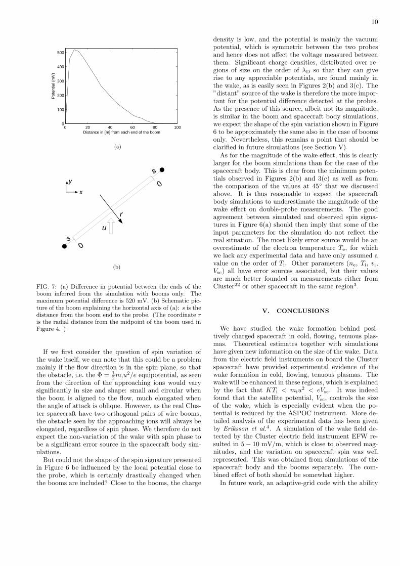
10

0 20 40 60 80 1000

100

200

300

400

500

Distance in [m] from each end of the boom

Pot

entia

l (m

V)

(a)

(b)

FIG. 7: (a) Difference in potential between the ends of theboom inferred from the simulation with booms only. Themaximum potential difference is 520 mV. (b) Schematic pic-ture of the boom explaining the horizontal axis of (a): s is thedistance from the boom end to the probe. (The coordinate r

is the radial distance from the midpoint of the boom used inFigure 4. )

If we first consider the question of spin variation ofthe wake itself, we can note that this could be a problemmainly if the flow direction is in the spin plane, so thatthe obstacle, i.e. the Φ = 1

2miu

2/e equipotential, as seenfrom the direction of the approaching ions would varysignificantly in size and shape: small and circular whenthe boom is aligned to the flow, much elongated whenthe angle of attack is oblique. However, as the real Clus-ter spacecraft have two orthogonal pairs of wire booms,the obstacle seen by the approaching ions will always beelongated, regardless of spin phase. We therefore do notexpect the non-variation of the wake with spin phase tobe a significant error source in the spacecraft body sim-ulations.

But could not the shape of the spin signature presentedin Figure 6 be influenced by the local potential close tothe probe, which is certainly drastically changed whenthe booms are included? Close to the booms, the charge

density is low, and the potential is mainly the vacuumpotential, which is symmetric between the two probesand hence does not affect the voltage measured betweenthem. Significant charge densities, distributed over re-gions of size on the order of λD so that they can giverise to any appreciable potentials, are found mainly inthe wake, as is easily seen in Figures 2(b) and 3(c). The”distant” source of the wake is therefore the more impor-tant for the potential difference detected at the probes.As the presence of this source, albeit not its magnitude,is similar in the boom and spacecraft body simulations,we expect the shape of the spin variation shown in Figure6 to be approximately the same also in the case of boomsonly. Nevertheless, this remains a point that should beclarified in future simulations (see Section V).

As for the magnitude of the wake effect, this is clearlylarger for the boom simulations than for the case of thespacecraft body. This is clear from the minimum poten-tials observed in Figures 2(b) and 3(c) as well as fromthe comparison of the values at 45◦ that we discussedabove. It is thus reasonable to expect the spacecraftbody simulations to underestimate the magnitude of thewake effect on double-probe measurements. The goodagreement between simulated and observed spin signa-tures in Figure 6(a) should then imply that some of theinput parameters for the simulation do not reflect thereal situation. The most likely error source would be anoverestimate of the electron temperature Te, for whichwe lack any experimental data and have only assumed avalue on the order of Ti. Other parameters (ne, Ti, vi,Vsc) all have error sources associated, but their valuesare much better founded on measurements either fromCluster22 or other spacecraft in the same region3.

V. CONCLUSIONS

We have studied the wake formation behind posi-tively charged spacecraft in cold, flowing, tenuous plas-mas. Theoretical estimates together with simulationshave given new information on the size of the wake. Datafrom the electric field instruments on board the Clusterspacecraft have provided experimental evidence of thewake formation in cold, flowing, tenuous plasmas. Thewake will be enhanced in these regions, which is explainedby the fact that KTi < miu

2 < eVsc. It was indeedfound that the satellite potential, Vsc, controls the sizeof the wake, which is especially evident when the po-tential is reduced by the ASPOC instrument. More de-tailed analysis of the experimental data has been givenby Eriksson et al.4. A simulation of the wake field de-tected by the Cluster electric field instrument EFW re-sulted in 5 − 10 mV/m, which is close to observed mag-nitudes, and the variation on spacecraft spin was wellrepresented. This was obtained from simulations of thespacecraft body and the booms separately. The com-bined effect of both should be somewhat higher.

In future work, an adaptive-grid code with the ability

11

to resolve finer structures, such as wire booms, should beused. Such a code would also allow to simulate any an-gle between the flow and the booms, making it possibleto obtain more reliable spin signatures. It would also berewarding to model a more realistic spacecraft geometrywith both body and booms, including important elec-tric elements close to the probes. The code should notbe implemented only with Dirichlet conditions, but withmore flexible boundary conditions. For this kind of prob-lem, Neumann conditions on all sides except the inflowingboundary are better suited. An example of such a codeis presented by Roussel et al.32. In spite of these desir-able improvements, the present study has shown that asimple and open source simulation code package can berun on a common desktop PC to give quantitative resultsfor this kind of spacecraft–plasma interaction problems.The main conclusions that can be drawn from this workare as follows.

1. The qualitative hypothesis of an electrostatic wakewith dimensions determined by the spacecraft po-tential field forming in situations with KTi <miu

2 < eVsc was quantitatively verified by simu-

lations.

2. Both the spacecraft body and the wire booms cre-ate large enhanced wakes in these situations. Theeffective size of the wire booms transverse to theflow can be increased from millimeters to meters.

3. The size of the wake scales with the plasma param-eters, of which the two most important features are:

(a) low ion temperature causes larger ion wake,and

(b) high electron temperature leads to more neg-ative potential in the wake.

4. The signatures from the electric field data agreewell with the simulations, and their shape and mag-nitude depends on plasma parameters. It is there-fore in principle possible to derive plasma param-eters from wake observations in electric field data.The first application of this has been presented byEngwall et al.22

1 A. W. Yau and M. Andre,Space Sci. Rev. 80, 1 (1997).2 T. E. Moore, C. R. Chappell, M. O. Chandler, P. D.

Craven, B. L. Giles, C. J. Pollock, J. L. Burch, D. T.Young, J. H. Waite Jr., J. E. Nordholt, M. F. Thom-sen, D. J. McComas, J. J. Berthelier, W. S. Williamson,R. Robson, and F. S. Mozer,Science 277, 349 (1997).

3 Y.-J. Su, J. L. Horwitz, T. E. Moore, B. L. Giles, M. O.Chandler, P. D. Craven, M. Hirahara, and C. J. Pollock,J. Geophys. Res. 103, 29 305 (1998).

4 A. Eriksson, M. Andre, B. Klecker, H. Laakso, P.-A. Lindqvist, F. Mozer, G. Paschmann, A. Pedersen,J. Quinn, R. Torbert, K. Torkar, and H. Vaith, Ann. Geo-phys. (in press), (2006).

5 Y. L. Al’pert, A. V. Gurevich, and L. P. Pitaevskii, SpacePhysics with Artificial Satellites (Consultants Bureau, NewYork, 1965).

6 D. E. Hastings, J. Geophys. Res. 100, 14 457 (1995).7 A. Pedersen, P. Decreau, P. Escoubet, G. Gustafsson,

H. Laakso, P.-A. Lindqvist, B. Lybekk, F. Mozer, andA. Vaivads, Ann. Geophys. 19, 1483 (2001).

8 L. Kraus and K. W. Watson, Phys. Fluids 1, 480 (1958).9 S. Rand, Phys. Fluids 3, 588 (1960).

10 S. D. Hester and A. A. Sonin, Phys. Fluids 13, 641 (1960).11 N. Singh and V. S. Chagani, J. Geophys. Res. 102, 195

(1997).12 L. Zinin, S. Grigoriev, and I. Rylina, Auroral phenom-

ena and solar-terrestrial relations: Proceedings of theconference in memory of Yuri Galperin, 2004, edited byM. L.M.Zelenyi and J.H.Allen, Eds. CAWSES Handbook-001, 2004, pp. 76–83.

13 J.-F. Roussel and J.-J. Berthelier, J. Geophys. Res. 109,A01104 (2004).

14 O. H. Bauer, R. Grard, G. Haerendel, and A. Pedersen,“Influence of wake and photoemission on electric field mea-

surements with a double probe on GEOS-2,” in Space-

craft/Plasma Interactions and their Influence on Field and

Particle Measurements, ser. ESA SP-198, 1983, pp. 51–56.15 A. Pedersen, C. A. Cattell, C.-G. Falthammar,

V. Formisano, P.-A. Lindqvist, F. Mozer, and R. Torbert,Space Sci. Rev. 37, 269 (1984).

16 E. Engwall, A. Eriksson, A. Pedersen, J. Forest,G. Paschmann, J. Quinn, R. Torbert, and K. Torkar,“Wake effects on positively charged spacecraft in flow-ing tenuous plasmas: Cluster observations and modeling,”in Proceedings of the 8th Spacecraft Charging Technology

Conference, Huntsville, Alabama, 2003.17 E. Engwall and A. I. Eriksson, “Cold magnetospheric

plasma flows and spacecraft wakes: PicUp3D simulationsand Cluster data,” in Proceedings of the 9th Spacecraft

Charging Technology Conference, Tsukuba, Japan, 2005.18 E. Engwall, “Numerical studies of spacecraft-plasma in-

teraction: Simulations of wake effects on the Clus-ter electric field instruments EFW,” Swedish Instituteof Space Physics,” IRF Scientific Report 284, 2004,http://www.irf.se/Publications/.

19 J. Forest, L. Eliasson, and A. Hilgers, “A new spacecraftplasma simulation software, PicUp3D/SPIS,” in 7th Space-

craft Charging Technology Conference, vol. SP-476. ESA,2001, pp. 515–520.

20 C. K. Birdsall and A. B. Langdon, Plasma Physics viaComputer Simulations (Adam Hilger, Bristol, 1991).

21 A. Pedersen, F. Mozer, and G. Gustafsson, “Electric fieldmeasurements in a tenuous plasma with spherical doubleprobes,” in Measurement Techniques in Space Plasmas:

Fields, ser. Geophysical Monograph 103. American Geo-physical Union, 1998, pp. 1–12.

22 E. Engwall, A. I. Eriksson, M. Andre, I. Dandouras,G. Paschmann, J. Quinn, and K. Torkar, Geophys. Res.

12

Lett. (accepted), (2006).23 A. Pedersen, Ann. Geophys. 13, 118 (1995).24 R. D. Sydora, “Low noise electromagnetic δf particle-in-

cell plasma simulation model and applications,” in Space

plasma simulation: proceedings of the Sixth International

School/Symposium, 2001.25 E. Hallen, Electromagnetic Theory, (Chapman & Hall,

London, 1962).26 L. D. Landau and E. M. Lifshitz, Course of Theoretical

Physics, vol. 1: Mechanics, 3rd ed. (Pergamon Press, NewYork, 1976).

27 C. P. Escoubet, M. Fehringer, and M. Goldstein, Ann. Geo-phys. 19, 1197 (2001).

28 G. Paschmann, C. E. McLlwain, J. M. Quinn, R. B. Tor-bert, and E. C. Whipple, “The Electron Drift Techniquefor Measuring Electric and Magnetic Fields,” in Measure-

ment Techniques in Space Plasmas: Fields, ser. Geophysi-cal Monograph 103. American Geophysical Union, 1998,

pp. 29–38.29 K. Torkar, W. Riedler, C. P. Escoubet, M. Fehringer,

R. Schmidt, R. J. L. Grard, H. Arends, F. Rudenauer,W. Steiger, B. T. Narheim, K. Svenes, R. Torbert,M. Andre, A. Fazakerley, R. Goldstein, R. C. Olsen,A. Pedersen, E. Whipple, and H. Zhao, Ann. Geophys. 19,1289 (2001).

30 R. H. Comfort, T. E. Moore, P. D. Craven, C. J. Pollock,F. S. Mozer, and W. T. Williamson, J. Spacecraft andRockets 35, 845 (1998).

31 N. Singh, W. C. Leung, T. E. Moore, and P. D. Craven,J. Geophys. Res. 106(A9), 19179 (2001).

32 J.-F. Roussel, F. Rogier, D. Volpert, J. Forest,G. Rousseau, and A. Hilgers, “Spacecraft plasma inter-action software (SPIS): Numerical solvers methods andarchitecture,” in Proceedings of the 9th Spacecraft Charg-

ing Technology Conference, Tsukuba, Japan, 2005.

Paper II

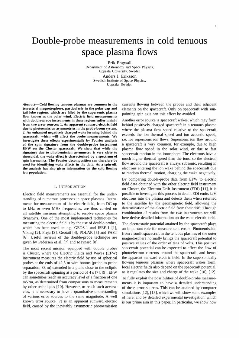
1

Double-probe measurements in cold tenuousspace plasma flows

Erik EngwallDepartment of Astronomy and Space Physics,

Uppsala University, Sweden

Anders I. ErikssonSwedish Institute of Space Physics,

Uppsala, Sweden

Abstract— Cold flowing tenuous plasmas are common in theterrestrial magnetosphere, particularly in the polar cap andtail lobe regions, which are filled by the supersonic plasmaflow known as the polar wind. Electric field measurementswith double-probe instruments in these regions suffer mainlyfrom two error sources: 1. An apparent sunward electric fielddue to photoemission asymmetries in the probe-boom system.2. An enhanced negatively charged wake forming behind thespacecraft, which will affect the probe measurements. Weinvestigate these effects experimentally by Fourier analysisof the spin signature from the double-probe instrumentEFW on the Cluster spacecraft. We show that while thesignature due to photoemission asymmetry is very close tosinusoidal, the wake effect is characterised by a spectrum ofspin harmonics. The Fourier decomposition can therefore beused for identifying wake effects in the data. As a spin-off,the analysis has also given information on the cold flowingion population.

I. INTRODUCTION

Electric field measurements are essential for the under-standing of numerous processes in space plasmas. Instru-ments for measurement of the electric field, from DC upto kHz or even MHz frequencies, are thus carried onall satellite missions attempting to resolve space plasmadynamics. One of the most implemented techniques formeasuring the electric field is by the use of double-probes,which has been used on e.g. GEOS-1 and ISEE-1 [1],Viking [2], Freja [3], Geotail [4], POLAR [5] and FAST[6]. Useful reviews of the double-probe technique aregiven by Pedersen et al. [7] and Maynard [8].

The most recent mission equipped with double probesis Cluster, where the Electric Fields and Waves (EFW)instrument measures the electric field by use of sphericalprobes at the ends of 42.5 m wire booms (probe-to-probeseparation: 88 m) extended in a plane close to the eclipticby the spacecraft spinning at a period of 4 s [7], [9]. EFWcan sometimes reach an accuracy level of a fraction of onemV/m, as determined from comparisons to measurementsby other techniques [10]. However, to reach such accura-cies, it is necessary to have a quantitative understandingof various error sources to the same magnitude. A wellknown error source [7] is an apparent sunward electricfield, caused by the inevitably asymmetric photoemission

currents flowing between the probes and their adjacentelements on the spacecraft. Only on spacecraft with sun-pointing spin axis can this effect be avoided.

Another error source is spacecraft wakes, which may formbehind positively charged spacecraft in a tenuous plasmawhere the plasma flow speed relative to the spacecraftexceeds the ion thermal speed and ion acoustic speed,i.e. for supersonic ion flows. Supersonic ion flow arounda spacecraft is very common, for example, due to highplasma flow speed in the solar wind, or due to fastspacecraft motion in the ionosphere. The electrons have amuch higher thermal speed than the ions, so the electronflow around the spacecraft is always subsonic, resulting inelectrons entering the ion wake behind the spacecraft dueto random thermal motion, charging the wake negatively.

By comparing double-probe data from EFW to electricfield data obtained with the other electric field instrumenton Cluster, the Electron Drift Instrument (EDI) [11], it ispossible to investigate this process in detail. EDI emits keVelectrons into the plasma and detects them when returnedto the satellite by the geomagnetic field, allowing thedetermination of the electric field from their drift. Throughcombination of results from the two instruments we willhere derive detailed information on the wake electric field.

The electrostatic potential attained by the spacecraft playsan important role for measurement errors. Photoemissionfrom a sunlit spacecraft in the tenuous plasmas of the outermagnetosphere normally brings the spacecraft potential topositive values of the order of tens of volts. This positivespacecraft potential can be expected to affect the flow ofphotoelectron currents around the spacecraft, and hencethe apparent sunward electric field. In the supersonicallyflowing tenuous plasmas where spacecraft wakes form,local electric fields also depend on the spacecraft potential,as it regulates the size and charge of the wake [10], [12].

To fully exploit the possibilities of double-probe measure-ments it is important to have a detailed understandingof these error sources. This can be attained by computersimulations [12], [13], which we will show some examplesof here, and by detailed experimental investigation, whichis our prime aim in this paper. In particular, we show how

2

the errors may be identified by the Fourier decompositionof the observed spin signature.

In this paper we examine the apparent sunward field dueto asymmetric photoemission and the wake field with theambition to be able to identify and remove spurious fieldsfrom EFW data. We also retrieve information about thecold plasma flow from the wake field.

II. SPACECRAFT WAKE AFFECTING DOUBLE-PROBE

INSTRUMENT

A. Evidence of wake in Cluster data

When operating in cold flowing plasmas, a direct interpre-tation of EFW data gives an electric field estimate differingfrom what is observed by EDI. An example from the polarwind is shown in Figure 1. In this Figure it can alsoclearly be seen that the problems grow when the spacecraftpotential is high.

The explanation to the difference between the instrumentsis that an enhanced wake is formed behind the spacecraft[10]. This wake will be much larger than expected fromthe geometrical size of the spacecraft, if the flow energyof the ions, Ei

k, not only exceeds the ion thermal energy,but also is lower than the spacecraft potential, i.e. if thefollowing inequality is satisfied

KTi < Eik < eVs, (1)

where KTi and Vs are the ion thermal energy and thespacecraft potential, respectively. For such conditions, theions will be deflected by the potential structures ratherthan the geometrical shape of the spacecraft. In addition,not only the spacecraft body will contribute to the wake,but also the thin wire booms, since their effective size willgrow from a few millimeters to the order of meters.

As the keV electrons emitted by EDI have a gyroradiimuch larger than the typical dimensions of any spacecraftwake size, and are only very weakly affected by therelatively small electrostatic potentials forming around thespacecraft, the electric field estimate from EDI is unaf-fected by the wake. On the other hand, the EFW probes,reaching only 44 m from the centre of the spacecraft, willoften clearly pick up the wake signature.

B. Simulations of the wake

To study the wake formation behind Cluster and theeffect on EFW, we have performed simulations with thecode package PicUp3D [14]. The simulations may alsoprovide some information on the dependence of the wakeproperties on plasma parameters such as ion temperature,which is useful since the cold ions are difficult to measurein situ with conventional ion detectors. We have run twotypes of simulations for typical polar wind conditionsmodelling the ions as protons (E i

k=10 eV, KTi=1-2 eV,

KTe=1-2 eV, n0=0.2 cm−3, Vs=35 V.): The wake effectbehind a) one pair of the wire booms only, and b) thespacecraft body only. This division is made to simplify thesimulations, but also to better understand the contributionsto the wake from different parts of the spacecraft system.The simulations with the booms have indeed shown thatthey can by themselves create a wake giving rise to a spu-rious electric field of over 5 mV/m, assuming the probesperfectly couple to the plasma [12]. This is comparable tothe spurious electric field in EFW data of 5-10 mV/m.

In Figure 2(a) the ion density from one of the simulationswith the spacecraft only is displayed, showing a cleardepletion behind the spacecraft. This ion wake will toa large extent be filled with electrons, whose thermalspeed greatly exceeds the flow speed, and a negativelycharged wake is created behind the spacecraft, whichcan be seen in Figure 2(b), where the potential contoursaround the spacecraft are shown. The effect on the double-probe instrument mounted on a spinning spacecraft fordifferent plasma parameters is shown in Figure 3, whichindeed show the same overall shape as EFW data. Fromthe simulations, it is evident that the size of the wake,as well as the signatures are dependent on the plasmaparameters. (For more details on the simulations and thedependence of wake properties on different parameters,see Engwall et al. [12].) Thus, by careful examination ofthe signatures of the spurious EFW signal in combinationwith the simulation results, there is a potential to deriveproperties of the flowing plasma. By another method,it is possible to calculate the flow velocity only fromcomparison between EFW and EDI data, provided thatcertain conditions apply [15]. In section III-B we show thatit is possible to determine the angle of the flowing plasmain the spin plane, and also the shape and depth of thewake by examination of the spin signature of the electricfield data only. From the sounding experiment WHISPERon Cluster [16], as well as from measurements of thespacecraft potential, the plasma density can be estimated.The remaining two free parameters, the electron andion temperatures, could possibly be obtained by carefulexamination of the signatures of the spurious EFW signalin comparison with the simulation results, assuming thatthe plasma flow consists of protons.

Eventhough protons consitute the dominant ion speciesin the polar wind, the O+ content can be relatively highduring magnetically active times. A flow rich in O+ willcertainly create another type of wake, since the O+ ionsare higher in energy than the protons [17]. This higherenergy will give rise to a more narrow wake, and thesignatures from the double-probe instrument should thusbe affected. In principle, the signatures could thereforealso tell something about the ratio of ion species inthe cold plasma flow. However, it might be difficult todistinguish variations due to ion content from variationsrelated to other plasma properties, such as proton andelectron temperatures.

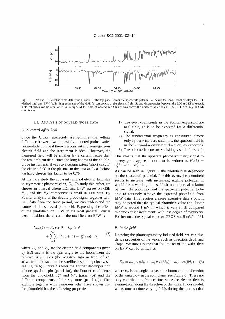
3

03:45 04:00 04:15 04:30 04:45

10

40V

ps [V

]

Cluster SC1 2001−02−14

03:45 04:00 04:15 04:30 04:45−15

−10

−5

0

Ex

[mV

/m]

Time [UT] on 2001−02−14

Fig. 1. EFW and EDI electric field data from Cluster 1. The top panel shows the spacecraft potential Vs, while the lower panel displays the EDI(dashed line) and EFW (solid line) estimates of the GSE X component of the electric field. Strong discrepancies between the EDI and EFW electricfield estimates can be seen when Vs is high. At the time of observation Cluster was above the northern polar cap at (-2.5, 1.4, 4.9) RE in GSEcoordinates.

III. ANALYSIS OF DOUBLE-PROBE DATA

A. Sunward offset field

Since the Cluster spacecraft are spinning, the voltagedifference between two oppositely mounted probes variessinusoidally in time if there is a constant and homogeneouselectric field and the instrument is ideal. However, themeasured field will be smaller by a certain factor thanthe real ambient field, since the long booms of the double-probe instruments always to a certain extent ”short circuit”the electric field in the plasma. In the data analysis below,we have chosen this factor to be 0.75.

At first, we study the apparent sunward electric field dueto asymmetric photoemission, Ea. To study this effect, wechoose an interval where EDI and EFW agrees on GSEEY , and the EX component is small in EDI data. ByFourier analysis of the double-probe signal together withEDI data from the same period, we can understand thenature of the sunward photofield. Expressing the effectof the photofield on EFW in its most general Fourierdecomposition, the effect of the total field on EFW is

Etot(θ) = Ex cos θ − Ey sin θ+

+

∞∑

n=1

(aphn

cos(nθ) + bphn

sin(nθ))(2)

where Ex and Ey are the electric field components givenby EDI and θ is the spin angle to the boom from thepositive XGSE axis (the negative sign in front of Ey

arises from the fact that the satellite is spinning clockwise,see Figure 6). Figure 4 shows the Fourier decompositionof one specific spin (panel (a)), the Fourier coefficientsfrom the photofield, aph

nand bph

n, (panel (b)) and the

different components of the signature (panel (c)). Thisexample together with numerous other have shown thatthe photofield has the following properties:

1) The even coefficients in the Fourier expansion arenegligible, as is to be expected for a differentialsignal.

2) The fundamental frequency is constituted almostonly by cos θ (b1 very small, i.e. the spurious field isin the sunward-antisunward direction, as expected).

3) The odd coefficients are vanishingly small for n > 1.

This means that the apparent photoasymmetry signal toa very good approximation can be written as Ea(θ) =aph1 cos θ = E0

a cos θ.

As can be seen in Figure 5, the photofield is dependenton the spacecraft potential. For this event, the photofieldseems to increase with increasing satellite potential. Itwould be rewarding to establish an empirical relationbetween the photofield and the spacecraft potential to beable to routinely remove the expected photofield fromEFW data. This requires a more extensive data study. Itmay be noted that the typical photofield value for ClusterEFW is around 1 mV/m, which is very small comparedto some earlier instruments with less degree of symmetry.For instance, the typical value on GEOS was 8 mV/m [18].

B. Wake field

Knowing the photoasymmetry induced field, we can alsoderive properties of the wake, such as direction, depth andshape. We now assume that the impact of the wake fieldon EFW can be written as

Ew = aw1 cos θb + aw3 cos(3θb) + aw5 cos(5θb), (3)

where θb is the angle between the boom and the directionof the wake flow in the spin plane (see Figure 6). There areonly contributions from cosine, since the electric field issymmetrical along the direction of the wake. In our model,we assume no time varying fields during the spin, so that

4

(a)

−0.3−0.1

−0.02

0.1

13


Grid

poi

nt in

x−

dire

ctio

n

0 20 40 60 80 1000

10

20

30

40

50

(b)

Fig. 2. Ion density and potential around the spacecraft. Thedashed circles show the location of the Cluster EFW probesthroughout a spin period. (The grid spacing is 2.7 m.) (a) Iondensity in the x − y-plane through the spacecraft. (The whitesquare shows the location of the spacecraft.) (b) Potential in thex−y-plane through the spacecraft, the potential of which is 35 V.The minimum value of the potential in the wake is −0.34 V.Equipotential contours are given at −0.3, −0.1, −0.01, 0.1, 1,3, 10 and 35 V.

when equating the potential difference all even Fouriercomponents vanish. We also neglect all terms higher thanfifth, which should be accurate for wide wakes (such asin Figure 2(a)). Narrow wakes occur for example in thesolar wind, but do not normally constitute a large problemsince they are easily detectable in EFW data.

Introducing θw as the angle between the positive XGSE

direction and the wake, the total electric field signaturecan be expressed as

Etot(θ) = (Ex + E0a + aw1 cos θw) cos θ+

+ (−Ey + aw1 sin θw) sin θ+

+ aw3 cos(3θw) cos(3θ) + aw3 sin(3θw) sin(3θ)+

+ aw5 cos(5θw) cos(5θ) + aw5 sin(5θw) sin(5θ).(4)

From a Fourier analysis of EFW spin data, we can nowretrieve the direction of the wake in the spin plane, θw,the wake Fourier components, aw1, aw3 and aw5, whichdescribes the depth and shape of the wake, and the ampli-

0 90 180 270 360−1000

−800

−600

−400

−200

0

200

400

600

800

1000

Angle [deg] of the boom relative to the plasma flow direction.

Pot

entia

l diff

eren

ce [m

V] b

etw

een

the

two

ends

of t

he b

oom

s.


Te=2 eV, T

i=1 eV

Te=2 eV, T

i=2 eV

Te=1 eV, T

i=1 eV

Te=1 eV, T

i=2 eV

EFW data

Fig. 3. Comparison of signatures from EFW data with four simulationswith the spacecraft. The signatures show the potential difference betweenthe probes at different angles of the boom relative to the flow. The EFWdata is taken from the difference between the opposite probes 3 and4 (probe pair 34) of the EFW instrument on Cluster 3 during one spinperiod (4 s) starting at 2002-02-13 01:48:06. In the simulations the space-craft potential and density are constant, Vs=35 V and n0=0.2 cm−3,while the temperatures are varied: 1. KTe = 2 eV, KTi = 1 eV. 2.KTe = KTi = 2 eV. 3. KTe = KTi = 1 eV. 4. KTe = 1 eV,KTi = 2 eV. The amplitude of the spurious electric field varies from4-10 mV/m.

tude of the photoelectron field, E0a . We make the Fourier

analysis of one spin at a time. As the EFW data gives sixFourier components, but only five variables, the systemof equations is overdetermined. We choose to derive θw

both from the third and fifth Fourier components, sinceit is not uniquely determined: θw3 can take 6 differentvalues (θw3 = 1

3arctan(b3/a3)+

nπ

3) and θw5 10 different

values (θw5 = 15

arctan(b5/a5) + nπ

5). The correct angle

is found by minimising the difference between θw3 andθw5. A small difference indicates that we have found theright angle and also confirms the validity of our model ofthe wake stated in equation (3). Figure 7 shows the EFWdata during one spin together with the photoelectron andwake fields.

Performing the Fourier analysis for a number of subse-quent spins, we can see how the wake direction changeswith time (see Figure 8(a)), but also investigate relationsbetween the satellite potential and the wake field (seeFigure 8(b)). As can be seen in Figure 8(a), the directionof the wake in the spin plane is almost anti-parallel withthe magnetic field component in the spin plane, which isexpected for small perpendicular electric fields implying aplasma flow mostly along the magnetic field. Figure 8(b)gives the ratios aw3/aw1 and aw5/aw1 as a function ofthe satellite potential. Both ratios tend to decrease as thesatellite potential increases, which confirms the model withan enhanced wake created by potential structures aroundthe satellite: for large potentials the wake grows biggerand the double-probe signal becomes more sinusoidal.

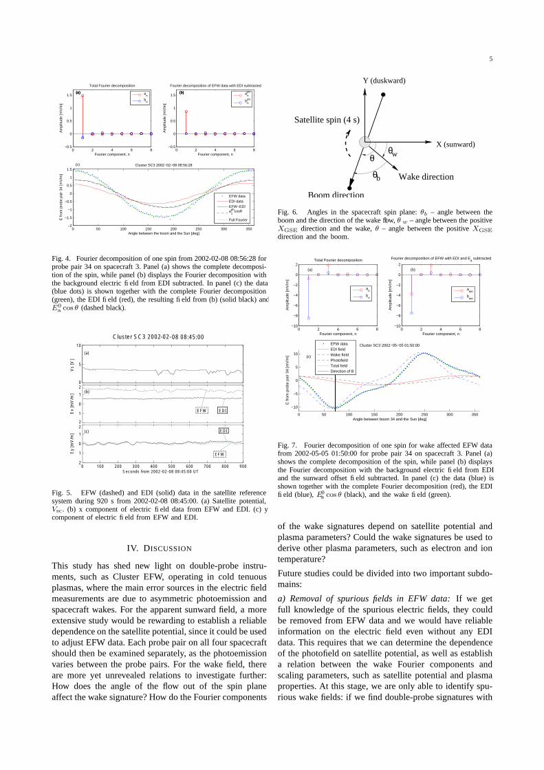
5

0 2 4 6 8−0.5

0

0.5

1

1.5

Fourier component, n

Am

plitu

de [m

V/m

]

Total Fourier decomposition

(a)(a)(a)

0 2 4 6 8−0.5

0

0.5

1

1.5


Am

plitu

de [m

V/m

]

Fourier decomposition of EFW data with EDI subtracted

(b)(b)(b)

0 50 100 150 200 250 300 350−2

−1.5

−1

−0.5

0

0.5

1

1.5Cluster SC3 2002−02−08 08:56:28

Angle between the boom and the Sun [deg]

E fr

om p

robe

pai

r 34

[mV

/m]

(c)

an

bn

anph

bnph

EFW dataEDI dataEFW−EDIa

1phcosθ

Full Fourier

Fig. 4. Fourier decomposition of one spin from 2002-02-08 08:56:28 forprobe pair 34 on spacecraft 3. Panel (a) shows the complete decomposi-tion of the spin, while panel (b) displays the Fourier decomposition withthe background electric field from EDI subtracted. In panel (c) the data(blue dots) is shown together with the complete Fourier decomposition(green), the EDI field (red), the resulting field from (b) (solid black) andE0

a cos θ (dashed black).

100 200 300 400 500 600 700 8000

5

10

Vs

[V ]

(a)

100 200 300 400 500 600 700 8002

1

0

1

2

Ex

[mV

/m] (b)

Cluster SC3 2002

-02-

08 08:45:00

0 100 200 300 400 500 600 700 800 900 2

1

0

1

2

Ey

[mV

/m] (c)

Seconds from 2002 -02 -08 08:45:00 UT

EDI

EFW

EDIEFW

Fig. 5. EFW (dashed) and EDI (solid) data in the satellite referencesystem during 920 s from 2002-02-08 08:45:00. (a) Satellite potential,Vsc. (b) x component of electric field data from EFW and EDI. (c) ycomponent of electric field from EFW and EDI.

IV. DISCUSSION

This study has shed new light on double-probe instru-ments, such as Cluster EFW, operating in cold tenuousplasmas, where the main error sources in the electric fieldmeasurements are due to asymmetric photoemission andspacecraft wakes. For the apparent sunward field, a moreextensive study would be rewarding to establish a reliabledependence on the satellite potential, since it could be usedto adjust EFW data. Each probe pair on all four spacecraftshould then be examined separately, as the photoemissionvaries between the probe pairs. For the wake field, thereare more yet unrevealed relations to investigate further:How does the angle of the flow out of the spin planeaffect the wake signature? How do the Fourier components

X (sunward)θwθ

θb Wake direction

Satellite spin (4 s)

Y (duskward)

Boom direction

Fig. 6. Angles in the spacecraft spin plane: θb – angle between theboom and the direction of the wake flow, θ w – angle between the positiveXGSE direction and the wake, θ – angle between the positive XGSE

direction and the boom.

0 2 4 6 8−10

−8

−6

−4

−2

0

2


Am

plitu

de [m

V/m

]

Total Fourier decomposition

(a)

an

bn

0 2 4 6 8−10

−8

−6

−4

−2

0

2


Am

plitu

de [m

V/m

]

Fourier decomposition of EFW with EDI and Ea subtracted

(b)

awn

bwn

0 50 100 150 200 250 300 350

−10

−5

0

5

10

Angle between boom 34 and the Sun [deg]

E fr

om p

robe

pai

r 34

[mV

/m]

Cluster SC3 2002−05−05 01:50:00

(c)

EFW dataEDI fieldWake fieldPhotofieldTotal fieldDirection of B

Fig. 7. Fourier decomposition of one spin for wake affected EFW datafrom 2002-05-05 01:50:00 for probe pair 34 on spacecraft 3. Panel (a)shows the complete decomposition of the spin, while panel (b) displaysthe Fourier decomposition with the background electric field from EDIand the sunward offset field subtracted. In panel (c) the data (blue) isshown together with the complete Fourier decomposition (red), the EDIfield (blue), E0

a cos θ (black), and the wake field (green).

of the wake signatures depend on satellite potential andplasma parameters? Could the wake signatures be used toderive other plasma parameters, such as electron and iontemperature?

Future studies could be divided into two important subdo-mains:

a) Removal of spurious fields in EFW data: If we getfull knowledge of the spurious electric fields, they couldbe removed from EFW data and we would have reliableinformation on the electric field even without any EDIdata. This requires that we can determine the dependenceof the photofield on satellite potential, as well as establisha relation between the wake Fourier components andscaling parameters, such as satellite potential and plasmaproperties. At this stage, we are only able to identify spu-rious wake fields: if we find double-probe signatures with

6

0 100 200 300 400 500 600 700 800 900

−50

0

50

100

150

200

250

300

350

Cluster SC3 2002−02−08 08:45:00

Seconds from 2002−02−08 08:45:00 UT

Dire

ctio

n re

lativ

e to

XG

SE [d

eg]

Angle of B in spin planeAngle of −B in spin planeAngle of B out of spin planeWake direction in spin plane

(a)

18 19 20 21 22 23 24 25 26−0.05

0

0.05

0.1

0.15

0.2

0.25

0.3

0.35

0.4Cluster SC3 2002−02−08 08:45:00

Satellite potential [V]

Quo

tient

s of

Fou

rier

com

pone

nts

aw3

/aw1

aw5

/aw1

(b)

Fig. 8. (a) Angles versus time: Derived angles of the wake (points),α = 360◦−∧(XGSE,B) in spin plane (dashed), α+180◦ (solid), andelevation angle of B out of the spin plane (dotted). (b) Dependence ofthe wake Fourier components on the satellite potential. Stars correspondsto aw3/aw1 , while circles represents aw5/aw1.

higher frequencies than the fundamental in the Fourierdecomposition, we can suspect that a wake has formedand thus treat the data with care.

b) Information about cold ions: As described in sectionII-B, the simulations together with data analysis fromdifferent instruments on Cluster could be used to deriveproperties of the wake. A first example can be found in[15], where the ion flow speed is calculated from the wakefield.

V. CONCLUSIONS

The main conclusions of the current study are:

1) We have shown that the sunward photoelectronfield contaminating double-probe measurements issinusoidal: Ea(θ) = E0

a cos θ.2) An enhanced wake forms downstream of a space-

craft in a flowing plasma, when the condition KTi <Ei

k < eVs is satisfied. Such a wake will affect adouble-probe electric field instrument significantly.

3) By Fourier analysis of the disturbed EFW signal, itis possible to determine the angle, width and depthof the wake.

4) The model for the wake field, Ew = aw1 cos θb +aw3 cos(3θb)+aw5 cos(5θb), is consistent with data.

5) Simulations with PicUp3D have given more infor-mation on the enhanced wake formation and haspermitted to quantify the effect on the double-probeelectric field instrument, assuming that the probesperfectly couple to the plasma. The magnitude aswell as the spin dependence of the wake field is ingood agreement with Cluster data. These simulationstogether with data analysis, can in principle be usedto derive properties of the cold ion flow.

VI. ACKNOWLEDGEMENTS

Electric field data from the EDI instrument (PI GoetzPaschmann) and magnetic field data from the FGM instru-ment (PI Elizabeth Lucek) has been used in the analysis.

REFERENCES

[1] A. Pedersen, C. A. Cattell, C.-G. Falthammar, V. Formisano, P.-A. Lindqvist, F. Mozer, and R. Torbert, “Quasistatic electric fieldmeasurements with spherical double probes on the GEOS and ISEEsatellites,” Space Science Reviews, vol. 37, pp. 269–312, 1984.

[2] L. P. Block, C.-G. Falthammar, P.-A. Lindqvist, G. Marklund, F. S.Mozer, A. Pedersen, T. A. Potemra, and L. J. Zanetti, “Electricfield measurements on Viking: first results,” Geophys. Res. Lett.,vol. 14, p. 435, 1987.

[3] G. Marklund, L. G. Blomberg, P.-A. Lindqvist, C.-G. Falthammar,G. Haerendel, F. Mozer, A. Pedersen, and P. Tanskanen, “The dou-ble probe electric field experiment on Freja: Experiment descriptionand first results,” Space Sci. Rev., vol. 70, pp. 483–508, 1994.

[4] K. Tsuruda, H. Hayakawa, M. Nakamura, T. Okada, A. Matsuoka,F. S. Mozer, and R. Schmidt, “Electric field measurements on theGEOTAIL satellite,” Journal of Geomagnetism and Geoelectricity,vol. 46, pp. 693–711, 1994.

[5] P. Harvey, F. S. Mozer, D. Pankow, J. Wygant, N. C. Maynard,H. Singer, W. Sullivan, P. B. Anderson, R. Pfaff, T. Aggson,A. Pedersen, C.-G. Falthammar, and P. Tanskanen, “The electricfield instrument on the Polar satellite,” Space Sci. Rev., vol. 71, pp.583–596, 1995.

[6] R. E. Ergun, C. W. Carlson, F. S. Mozer, G. T. Delory, M. Temerin,J. P. McFadden, D. Pankow, R. Abiad, P. Harvey, R. Wilkes,H. Primbsch, R. Elphic, R. Strangeway, R. Pfaff, and C. A. Cattell,“The FAST Satellite Fields Instrument,” Space Science Reviews,vol. 98, pp. 67–91, Aug. 2001.

[7] A. Pedersen, F. Mozer, and G. Gustafsson, “Electric field mea-surements in a tenuous plasma with spherical double probes,” inMeasurement Techniques in Space Plasmas: Fields, ser. Geophys-ical Monograph 103. American Geophysical Union, 1998, pp.1–12.

[8] N. C. Maynard, “Electric field measurements in moderate to highdensity space plasmas with passive double probes,” in MeasurementTechniques in Space Plasmas: Fields (AGU Geophysical Mono-graph 103), J. Borovsky, R. Pfaff, and D. Young, Eds. AmericanGeophysical Union, 1998, pp. 13–27.

[9] G. Gustafsson, M. Andre, T. Carozzi, A. I. Eriksson, C.-G. Faltham-mar, R. Grard, G. Holmgren, J. A. Holtet, N. Ivchenko, T. Karlsson,Y. Khotyaintsev, S. Klimov, H. Laakso, P.-A. Lindqvist, B. Lybekk,G. Marklund, F. Mozer, K. Mursula, A. Pedersen, B. Popielawska,S. Savin, K. Stasiewicz, P. Tanskanen, A. Vaivads, and J.-E.Wahlund, “First results of electric field and density observationsby Cluster EFW based on initial months of operation,” AnnalesGeophysicae, vol. 19, pp. 1219–1240, 2001.

7

[10] A. Eriksson, M. Andre, B. Klecker, H. Laakso, P.-A. Lindqvist,F. Mozer, G. Paschmann, A. Pedersen, J. Quinn, R. Torbert,K. Torkar, and H. Vaith, “Electric field measurements on Cluster:Comparing the double-probe and electron drift technique,” AnnalesGeophysicae, 2006, in press.

[11] G. Paschmann, J. M. Quinn, R. B. Torbert, H. Vaith, C. E.McIlwain, G. Haerendel, O. H. Bauer, T. Bauer, W. Baumjohann,W. Fillius, M. Forster, S. Frey, E. Georgescu, S. S. Kerr, C. A.Kletzing, H. Matsui, P. Puhl-Quinn, and E. C. Whipple, “TheElectron Drift Instrument on Cluster: overview of first results,”Annales Geophysicae, vol. 19, pp. 1273–1288, 2001.

[12] E. Engwall, A. I. Eriksson, and J. Forest, “Wake formation behindpositively charged spacecraft in flowing tenuous plasmas,” Physicsof Plasmas, 2006, in review.

[13] C. M. Cully and R. E. Ergun, “A quantitative look at double-probeelectric field measurements,” 2005, manuscript in preparation.

[14] J. Forest, L. Eliasson, and A. Hilgers, “A new spacecraft plasmasimulation software, PicUp3D/SPIS,” in 7 th Spacecraft ChargingTechnology Conference, vol. SP-476. ESA, 2001, pp. 515–520.

[15] E. Engwall, A. I. Eriksson, M. Andre, I. Dandouras, G. Paschmann,J. Quinn, and K. Torkar, “Low-energy (order 10 ev) ion flowin the magnetotail inferred from spacecraft wake observations,”Geophysical Research Letters, 2006, accepted.

[16] P. M. E. Decreau, P. Fergeau, V. Krasnoselskikh, E. Le Guirriec,M. Leveque, P. Martin, O. Randriamboarison, J. L. Rauch, F. X.Sene, H. C. Seran, J. G. Trotignon, P. Canu, N. Cornilleau,H. de Feraudy, H. Alleyne, K. Yearby, P. B. Mogensen, G. Gustafs-son, M. Andre, D. C. Gurnett, F. Darrouzet, J. Lemaire, C. C.Harvey, P. Travnicek, and Whisper experimenters, “Early resultsfrom the WHISPER instrument on Cluster: an overview,” AnnalesGeophysicae, vol. 19, pp. 1241–1258, 2001.

[17] Y.-J. Su, J. L. Horwitz, T. E. Moore, B. L. Giles, M. O. Chandler,P. D. Craven, M. Hirahara, and C. J. Pollock, “Polar wind surveywith the Thermal Ion Dynamics Experiment/Plasma Source Instru-ment suite aboard POLAR,” Journal of Geophysical Research, vol.103, pp. 29 305–29 337, 1998.

[18] A. Pedersen, R. Grard, K. Knott, D. Jones, A. Gonfalcone, andU. Fahleson, “Measurements of quasi-static electric fields between3 and 7 Earth radii on Geos-1,” Space Science Reviews, vol. 22,pp. 333–346, 1978.

Paper III

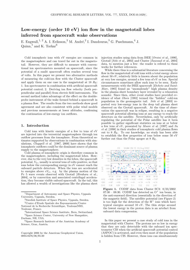
GEOPHYSICAL RESEARCH LETTERS, VOL. ???, XXXX, DOI:10.1029/,

Low-energy (order 10 eV) ion flow in the magnetotail lobes

inferred from spacecraft wake observations

E. Engwall,1, 2 A. I. Eriksson,2 M. Andre,2 I. Dandouras,3 G. Paschmann,4 J.

Quinn,5 and K. Torkar6

Cold ionospheric ions with eV energies are common inthe magnetosphere and can travel far out in the magneto-tail. However, they are difficult to measure with conven-tional ion spectrometers mounted on spacecraft, since thepotential of a sunlit spacecraft often reaches several tensof volts. In this paper we present two alternative methodsof measuring the cold-ion flow with the Cluster spacecraftand apply them on one case in the magnetotail at 18 RE:1. Ion spectrometer in combination with artificial spacecraftpotential control; 2. Deriving ion flow velocity (both per-pendicular and parallel) from electric field instruments. Thesecond method takes advantage of the effect on the double-probe instrument of the wake formed behind a spacecraft ina plasma flow. The results from the two methods show goodagreement and are also consistent with polar wind modelsand previous measurements at lower altitudes, confirmingthe continuation of low-energy ion outflows.

1. Introduction

Cold ions with kinetic energies of a few to tens of eVare injected into the terrestrial magnetosphere through ionoutflow processes from the ionosphere. From theoretical es-timates supported by observations in combination with sim-ulations, Chappell et al. [1987, 2000] have shown that theionospheric outflows could be the dominant source of plasmasupply to the magnetosphere.

Cold plasma of ionospheric origin is therefore common inthe magnetosphere, including the magnetotail lobes. How-ever, due to the very low densities in the lobes, the spacecraftpotential, Vsc, usually is several tens of volts positive, so thations below the corresponding energy in eV cannot reach theonboard particle detectors. When the ions are acceleratedto energies above eVsc, e.g. by the plasma motion of thePc 5 wave events observed with Geotail [Hirahara et al.,2004], or by convection and associated centrifugal accelera-tion, they become visible onbord spacecraft. In the tail, thishas allowed a wealth of investigations like the plasma sheet

1Department of Astronomy and Space Physics, UppsalaUniversity, Uppsala, Sweden.

2Swedish Institute of Space Physics, Uppsala, Sweden.3Centre d’Etude Spatiale des Rayonnements/Centre

National de la Recherche Scientifique, ToulouseNRS,Toulouse, France.

4International Space Science Institute, Bern, Switzerland.5Space Science Center, University of New Hampshire,

Durham, NH, USA.6Space Research Institute of the Austrian Academy of

Science, Graz, Austria.

Copyright 2006 by the American Geophysical Union.0094-8276/06/$5.00

injection studies using data from ISEE [Orsini et al., 1990],Geotail [Seki et al., 2002] and Cluster [Sauvaud et al., 2004]data, to mention just a few: the reader is refered to theseworks for further references.

While there thus is a substantial literature concerning theflow in the magnetotail of cold ions with a total energy aboveabout 50 eV, relatively little is known about the populationat very low energies, around a few tens of eV or less. Specialcircumstances sometimes allow such ions to be seen. Earlymeasurements with the ISEE spacecraft [Etcheto and Saint-Marc, 1985] found an “anomalously” high plasma densityin the plasma sheet boundary layer revealed by a relaxationsounder. Since then, other event studies have provided ev-idence of what Olsen [1982] termed the “hidden” cold-ionpopulation in the geomagnetic tail. Seki et al. [2003] re-ported very low-energy ions in the deep tail plasma sheetobserved on the Geotail spacecraft. At the time of obser-vation the spacecraft was in eclipse, resulting in a negativespacecraft potential allowing ions at any energy to reach thedetectors on the satellite. Nevertheless, only by artificiallyregulating the potential of the Polar satellite has it beenpossible to gather significant statistics on ions at or belowa few tens of eV, presented by Moore et al. [1997] and Suet al. [1998] in their studies of ionospheric cold plasma flowsout to 8 RE. To our knowledge, no study has been ableto establish the flow properties of ions below some 50 eVfurther out than the Polar apogee at 8 RE.

Figure 1. CODIF data from Cluster SC3: 8/23/200207:30 – 08:30. CODIF has detected an O+ ion beam, inthe anti-sunward direction (essentially in the direction ofthe magnetic field). The satellite potential (see Figure 2)is too high for the detection of the H+ ions which havetypical energies around 10 eV. The thin stripe aroundthe lowest energy in the proton data is an artefact fromonboard data compression.

In this paper we present a case study of cold ions in themagnetotail with Cluster. The protons are so low in energythat they are only detectable with the onboard ion spec-trometer CIS when the artificial spacecraft potential control(ASPOC) is activated, and even then most of the populationis hidden from CIS. However, these ions can simultaneously

1

X - 2 ENGWALL ET AL.: LOW-ENERGY ION FLOW IN MAGNETOTAIL

be indirectly detected with the electric field instruments,EFW and EDI, from the wake formed behind another of thefour Cluster spacecraft. We first show evidence for cold-ionflows in both ion and electric field data, and then derive theflow properties from these data.

2. Analysis of Particle Data

CIS consists of two different instruments: the mass-separating instrument CODIF, which was used in this study,and the hot-ion analyzer, HIA [Reme et al., 2001]. Figure1 shows CODIF data from spacecraft 3 (henceforth denotedSC3) collected during 1 hour, when the Cluster spacecraftare around [-17, -3, 5] RE GSM, i.e. in the northern lobe ofthe geomagnetic tail. The CODIF data show no outflowingprotons, but a distinct 100 eV (relative to the spacecraftpotential) cold oxygen flow directed mainly anti-parallel tothe magnetic field (B ≈ [37, 1, 7] nT in GSE coordinates).As can be seen in Figure 2, the satellite potential on SC3varies between 40 V and over 60 V, making it impossible forCODIF to detect any ions at lower energies. As a result, theplasma densities inferred from the HIA (Figure 2(b), solidlines) are much lower than the plasma density derived fromthe spacecraft potential by the method of Pedersen et al.[2001] (Figure 2(b), dashed line). On SC4 ASPOC [Torkaret al., 2001] is operating reducing the spacecraft potentialto 7 V and the data thus reveal a population of cold H+

ions. In addition, CODIF on SC4 is in retarding potentialanalyzer (RPA) mode, making it possible to measure lowenergies (0.7-25 eV) with high resolution [Dandouras, 2005].We assumed that the plasma properties were constant overspacecraft separation distances of typically 3400 km (on fieldlines around 3000 km).

07:30 07:40 07:50 08:00 08:10

20406080

Vs [V

]

UT

Cluster SC1 and SC3 2002−08−23 07:30:00

EFW (SC1) EFW (SC3)

07:30 07:40 07:50 08:00 08:10

0.02

0.1

1

n [c

m−

3 ]

UT

CIS (SC1) CIS (SC3) EFW (SC1)

−5

0

5

UT

Ex

[mV

/m]

07:30 07:40 07:50 08:00 08:10 08:20 08:30

−5

0

5

Ey

[mV

/m]

UT

EFW (SC3) EDI (SC3)

(a)

(b)

(c)

(d)

Figure 2. Data from Cluster SC1 and SC3: 8/23/200207:30 – 08:30. (a) Spacecraft potential derived fromEFW. (The spacecraft potential is higher on SC3 than onSC1 due to the operation of EDI on SC3.) (b) HIA den-sity measurements together with the density estimatedfrom the spacecraft potential on SC1 according to Ped-ersen et al. [2001]. (c), (d) Electric field measurements.

Figure 3 shows the distribution function from SC4 forH+ in the GSE vx − vz-plane (vy = 0). The distributionfunction has been corrected for the spacecraft potential of7 V, since CODIF measures the energy of the ions relativeto the spacecraft potential. From the figure we see that thehydrogen flow is aligned with the magnetic field, and has avelocity of 40 km/s (corresponding to 9 eV flow energy).

The oxygen flow has too high an energy to be measured

by CODIF on SC4 (in RPA mode), and was therefore de-

termined from the distribution function on SC3. After cor-

rection for the 40-60 V spacecraft potential, we obtained a

flow velocity with an anti-sunward component of around 30

to 35 km/s (vz is not reliable due to anode problems on

SC3, and we therefore disregarded this component; and vy

fluctuates around 0 km/s).

Bxz

Figure 3. The distribution function for H+ cut in thevx−vz-plane for vy = 0, averaged over 75 spins from 07:40to 07:45 on SC4. The velocities have been corrected forthe spacecraft potential of 7 V. The lowest velocities aremissing due to the instrument low-energy cutoff at 0.7 eV.Bxz is the magnetic field projected in the x − z-plane.

3. Analysis of Electric Field Data

Evidence of cold flowing ions can also be found in elec-

tric field data from SC3 for the same event. Cluster car-

ries two instruments for measurements of electric fields us-

ing different techniques: the double-probe instrument EFW

[Gustafsson et al., 1997] and the electron drift instrument

EDI [Paschmann et al., 1997]. The difference between the

EDI and EFW data, which can be seen in Figure 2(c) and

(d), is due to a potential created in a wake behind the space-

craft.

A wake will form behind a spacecraft for supersonic ion

flows, i.e. Wi > KTi, where Wi is the bulk ion flow energy

and KTi the thermal energy. If, in addition, the plasma is

sufficiently tenuous, the spacecraft potential will exceed the

ion flow energy, resulting in eVs > Wi > KTi. This creates

an enhanced wake, since in this case the ions are deflected

by the potential structures around the spacecraft [Eriksson

et al., 2006]. For Debye lengths greater than the spacecraft

dimensions the wake can be significantly enlarged, as has

been verified by particle-in-cell simulations [Engwall , 2004;

Engwall and Eriksson, 2006]. Figure 4 shows schematically

the wake formation in supersonic flows. In the case of an

enhanced wake the ion density will be largely depleted be-

hind the spacecraft. The ion wake will, to a large extent, be

filled with subsonic electrons, creating a negative potential

in the wake. The EFW probes, which are mounted on 44 m

wire booms (probe-to-probe separation 88 m), will observe

this negative potential, while the keV electron beam from

EDI is unaffected.

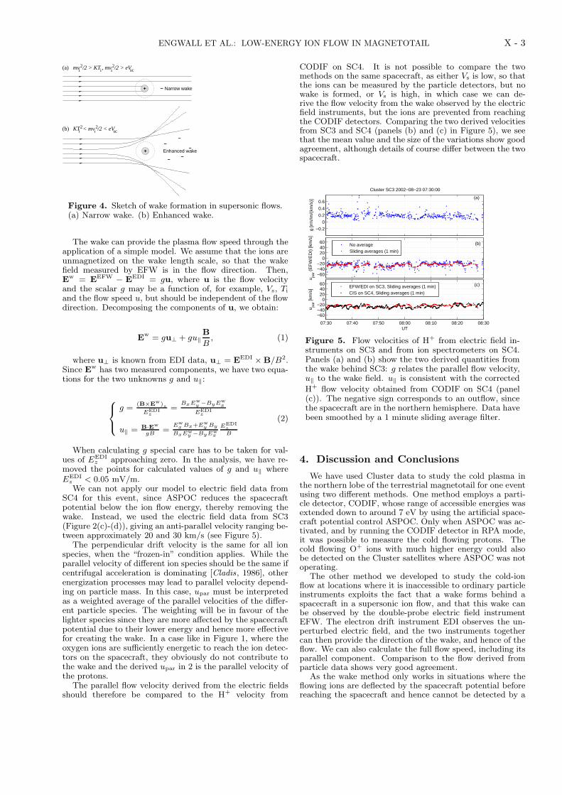
ENGWALL ET AL.: LOW-ENERGY ION FLOW IN MAGNETOTAIL X - 3

i i i scmv /2 > KT , mv /2 > eV2 2

KT < mv /2 < eVi i sc2 2

+ − Narrow wake

−

−−

−

+−

Enhanced wake

(b)

(a)

Figure 4. Sketch of wake formation in supersonic flows.(a) Narrow wake. (b) Enhanced wake.

The wake can provide the plasma flow speed through theapplication of a simple model. We assume that the ions areunmagnetized on the wake length scale, so that the wakefield measured by EFW is in the flow direction. Then,Ew = EEFW

− EEDI = gu, where u is the flow velocityand the scalar g may be a function of, for example, Vs, Ti

and the flow speed u, but should be independent of the flowdirection. Decomposing the components of u, we obtain:

Ew = gu⊥ + gu‖

B

B, (1)

where u⊥ is known from EDI data, u⊥ = EEDI× B/B2.

Since Ew has two measured components, we have two equa-tions for the two unknowns g and u‖:

g =(B×E

w)z

EEDIz

=BxEw

y−ByEw

x

EEDIz

u‖ = B·Ew

gB=

Ew

xBx+Ew

yBy

BxEwy−ByEw

x

EEDI

z

B

(2)

When calculating g special care has to be taken for val-ues of EEDI

z approaching zero. In the analysis, we have re-moved the points for calculated values of g and u‖ whereEEDI

z < 0.05 mV/m.We can not apply our model to electric field data from

SC4 for this event, since ASPOC reduces the spacecraftpotential below the ion flow energy, thereby removing thewake. Instead, we used the electric field data from SC3(Figure 2(c)-(d)), giving an anti-parallel velocity ranging be-tween approximately 20 and 30 km/s (see Figure 5).

The perpendicular drift velocity is the same for all ionspecies, when the “frozen-in” condition applies. While theparallel velocity of different ion species should be the same ifcentrifugal acceleration is dominating [Cladis, 1986], otherenergization processes may lead to parallel velocity depend-ing on particle mass. In this case, upar must be interpretedas a weighted average of the parallel velocities of the differ-ent particle species. The weighting will be in favour of thelighter species since they are more affected by the spacecraftpotential due to their lower energy and hence more effectivefor creating the wake. In a case like in Figure 1, where theoxygen ions are sufficiently energetic to reach the ion detec-tors on the spacecraft, they obviously do not contribute tothe wake and the derived upar in 2 is the parallel velocity ofthe protons.

The parallel flow velocity derived from the electric fieldsshould therefore be compared to the H+ velocity from

CODIF on SC4. It is not possible to compare the twomethods on the same spacecraft, as either Vs is low, so thatthe ions can be measured by the particle detectors, but nowake is formed, or Vs is high, in which case we can de-rive the flow velocity from the wake observed by the electricfield instruments, but the ions are prevented from reachingthe CODIF detectors. Comparing the two derived velocitiesfrom SC3 and SC4 (panels (b) and (c) in Figure 5), we seethat the mean value and the size of the variations show goodagreement, although details of course differ between the twospacecraft.

07:30 07:40 07:50 08:00 08:10

−0.2

0

0.2

0.4

0.6

g [m

V/m

/(km

/s)]

UT

Cluster SC3 2002−08−23 07:30:00

07:30 07:40 07:50 08:00 08:10

−60−40−20

0204060

UT

u par (

EF

W/E

DI)

[km

/s]

No averageSliding averages (1 min)

07:30 07:40 07:50 08:00 08:10 08:20 08:30

−60−40−20

0204060

UT

u par [k

m/s

] EFW/EDI on SC3, Sliding averages (1 min)CIS on SC4, Sliding averages (1 min)

(a)

(b)

(c)

Figure 5. Flow velocities of H+ from electric field in-struments on SC3 and from ion spectrometers on SC4.Panels (a) and (b) show the two derived quantities fromthe wake behind SC3: g relates the parallel flow velocity,u‖ to the wake field. u‖ is consistent with the corrected

H+ flow velocity obtained from CODIF on SC4 (panel(c)). The negative sign corresponds to an outflow, sincethe spacecraft are in the northern hemisphere. Data havebeen smoothed by a 1 minute sliding average filter.

4. Discussion and Conclusions

We have used Cluster data to study the cold plasma inthe northern lobe of the terrestrial magnetotail for one eventusing two different methods. One method employs a parti-cle detector, CODIF, whose range of accessible energies wasextended down to around 7 eV by using the artificial space-craft potential control ASPOC. Only when ASPOC was ac-tivated, and by running the CODIF detector in RPA mode,it was possible to measure the cold flowing protons. Thecold flowing O+ ions with much higher energy could alsobe detected on the Cluster satellites where ASPOC was notoperating.

The other method we developed to study the cold-ionflow at locations where it is inaccessible to ordinary particleinstruments exploits the fact that a wake forms behind aspacecraft in a supersonic ion flow, and that this wake canbe observed by the double-probe electric field instrumentEFW. The electron drift instrument EDI observes the un-perturbed electric field, and the two instruments togethercan then provide the direction of the wake, and hence of theflow. We can also calculate the full flow speed, including itsparallel component. Comparison to the flow derived fromparticle data shows very good agreement.

As the wake method only works in situations where theflowing ions are deflected by the spacecraft potential beforereaching the spacecraft and hence cannot be detected by a

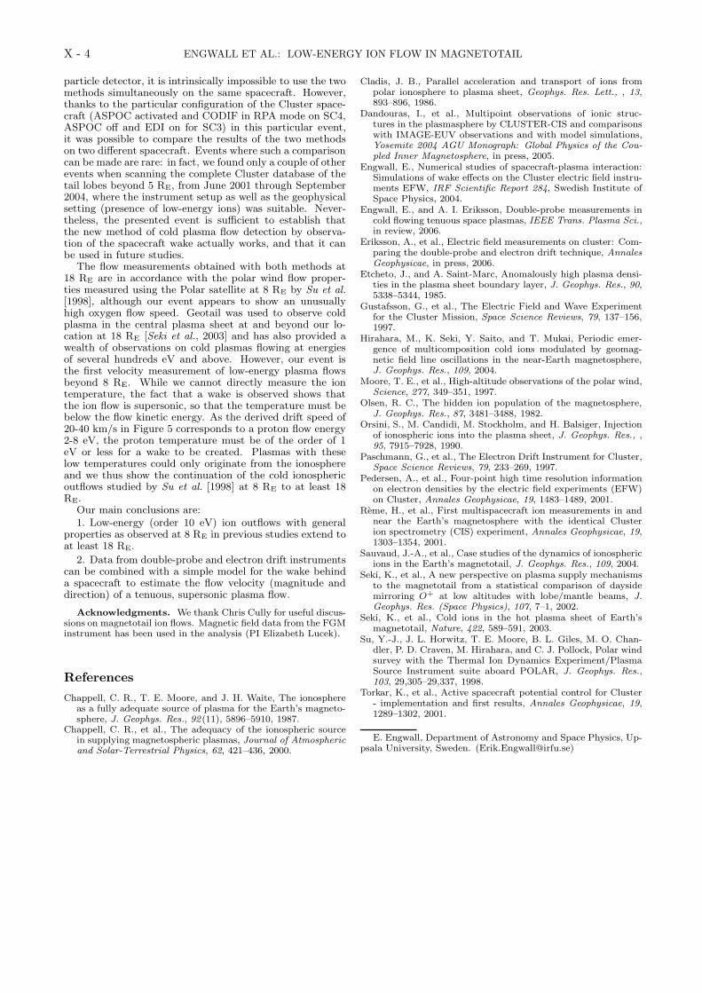
X - 4 ENGWALL ET AL.: LOW-ENERGY ION FLOW IN MAGNETOTAIL

particle detector, it is intrinsically impossible to use the twomethods simultaneously on the same spacecraft. However,thanks to the particular configuration of the Cluster space-craft (ASPOC activated and CODIF in RPA mode on SC4,ASPOC off and EDI on for SC3) in this particular event,it was possible to compare the results of the two methodson two different spacecraft. Events where such a comparisoncan be made are rare: in fact, we found only a couple of otherevents when scanning the complete Cluster database of thetail lobes beyond 5 RE, from June 2001 through September2004, where the instrument setup as well as the geophysicalsetting (presence of low-energy ions) was suitable. Never-theless, the presented event is sufficient to establish thatthe new method of cold plasma flow detection by observa-tion of the spacecraft wake actually works, and that it canbe used in future studies.

The flow measurements obtained with both methods at18 RE are in accordance with the polar wind flow proper-ties measured using the Polar satellite at 8 RE by Su et al.[1998], although our event appears to show an unusuallyhigh oxygen flow speed. Geotail was used to observe coldplasma in the central plasma sheet at and beyond our lo-cation at 18 RE [Seki et al., 2003] and has also provided awealth of observations on cold plasmas flowing at energiesof several hundreds eV and above. However, our event isthe first velocity measurement of low-energy plasma flowsbeyond 8 RE. While we cannot directly measure the iontemperature, the fact that a wake is observed shows thatthe ion flow is supersonic, so that the temperature must bebelow the flow kinetic energy. As the derived drift speed of20-40 km/s in Figure 5 corresponds to a proton flow energy2-8 eV, the proton temperature must be of the order of 1eV or less for a wake to be created. Plasmas with theselow temperatures could only originate from the ionosphereand we thus show the continuation of the cold ionosphericoutflows studied by Su et al. [1998] at 8 RE to at least 18RE.

Our main conclusions are:1. Low-energy (order 10 eV) ion outflows with general

properties as observed at 8 RE in previous studies extend toat least 18 RE.

2. Data from double-probe and electron drift instrumentscan be combined with a simple model for the wake behinda spacecraft to estimate the flow velocity (magnitude anddirection) of a tenuous, supersonic plasma flow.

Acknowledgments. We thank Chris Cully for useful discus-sions on magnetotail ion flows. Magnetic field data from the FGMinstrument has been used in the analysis (PI Elizabeth Lucek).

References

Chappell, C. R., T. E. Moore, and J. H. Waite, The ionosphereas a fully adequate source of plasma for the Earth’s magneto-sphere, J. Geophys. Res., 92 (11), 5896–5910, 1987.

Chappell, C. R., et al., The adequacy of the ionospheric sourcein supplying magnetospheric plasmas, Journal of Atmosphericand Solar-Terrestrial Physics, 62, 421–436, 2000.

Cladis, J. B., Parallel acceleration and transport of ions frompolar ionosphere to plasma sheet, Geophys. Res. Lett., , 13,893–896, 1986.

Dandouras, I., et al., Multipoint observations of ionic struc-tures in the plasmasphere by CLUSTER-CIS and comparisonswith IMAGE-EUV observations and with model simulations,Yosemite 2004 AGU Monograph: Global Physics of the Cou-pled Inner Magnetosphere, in press, 2005.

Engwall, E., Numerical studies of spacecraft-plasma interaction:Simulations of wake effects on the Cluster electric field instru-ments EFW, IRF Scientific Report 284, Swedish Institute ofSpace Physics, 2004.

Engwall, E., and A. I. Eriksson, Double-probe measurements incold flowing tenuous space plasmas, IEEE Trans. Plasma Sci.,in review, 2006.

Eriksson, A., et al., Electric field measurements on cluster: Com-paring the double-probe and electron drift technique, AnnalesGeophysicae, in press, 2006.

Etcheto, J., and A. Saint-Marc, Anomalously high plasma densi-ties in the plasma sheet boundary layer, J. Geophys. Res., 90,5338–5344, 1985.

Gustafsson, G., et al., The Electric Field and Wave Experimentfor the Cluster Mission, Space Science Reviews, 79, 137–156,1997.

Hirahara, M., K. Seki, Y. Saito, and T. Mukai, Periodic emer-gence of multicomposition cold ions modulated by geomag-netic field line oscillations in the near-Earth magnetosphere,J. Geophys. Res., 109, 2004.

Moore, T. E., et al., High-altitude observations of the polar wind,Science, 277, 349–351, 1997.

Olsen, R. C., The hidden ion population of the magnetosphere,J. Geophys. Res., 87, 3481–3488, 1982.

Orsini, S., M. Candidi, M. Stockholm, and H. Balsiger, Injectionof ionospheric ions into the plasma sheet, J. Geophys. Res., ,95, 7915–7928, 1990.

Paschmann, G., et al., The Electron Drift Instrument for Cluster,Space Science Reviews, 79, 233–269, 1997.

Pedersen, A., et al., Four-point high time resolution informationon electron densities by the electric field experiments (EFW)on Cluster, Annales Geophysicae, 19, 1483–1489, 2001.

Reme, H., et al., First multispacecraft ion measurements in andnear the Earth’s magnetosphere with the identical Clusterion spectrometry (CIS) experiment, Annales Geophysicae, 19,1303–1354, 2001.

Sauvaud, J.-A., et al., Case studies of the dynamics of ionosphericions in the Earth’s magnetotail, J. Geophys. Res., 109, 2004.

Seki, K., et al., A new perspective on plasma supply mechanismsto the magnetotail from a statistical comparison of daysidemirroring O+ at low altitudes with lobe/mantle beams, J.Geophys. Res. (Space Physics), 107, 7–1, 2002.

Seki, K., et al., Cold ions in the hot plasma sheet of Earth’smagnetotail, Nature, 422, 589–591, 2003.

Su, Y.-J., J. L. Horwitz, T. E. Moore, B. L. Giles, M. O. Chan-dler, P. D. Craven, M. Hirahara, and C. J. Pollock, Polar windsurvey with the Thermal Ion Dynamics Experiment/PlasmaSource Instrument suite aboard POLAR, J. Geophys. Res.,103, 29,305–29,337, 1998.

Torkar, K., et al., Active spacecraft potential control for Cluster- implementation and first results, Annales Geophysicae, 19,1289–1302, 2001.

E. Engwall, Department of Astronomy and Space Physics, Up-psala University, Sweden. ([email protected])

Cold magnetospheric plasma flows: Properties and interaction ...

Documents

Transcript of Cold magnetospheric plasma flows: Properties and interaction ...