1

Gas Distribution Mapping of Multiple Odour

Sources using a Mobile RobotAmy Loutfi, Silvia Coradeschi, Achim J. Lilienthal and Javier Gonzalez

Abstract

Mobile olfactory robots can be used in a number of relevant application areas where a better understanding of agas distribution is needed, such as environmental monitoring and safety and security related fields. In this paper we

present a method to integrate the classification of odours together with gas distribution mapping. The resulting odourmap is then correlated with the spatial information collected from a laser range scanner to form a combined map.

Experiments are performed using a mobile robot in large and unmodified indoor and outdoor environments. Multipleodour sources are used and are identified using only transient information from the gas sensor response. The resulting

multi level map can be used as a representation of the collected odour data.

I. INTRODUCTION

The combination of gas sensors on mobile robots is useful for a number of application areas within safety,

security and environmental inspection. Instead of using humans, a robot can be dispatched to areas of contaminous

odours for inspection, or can provide continuous monitoring of an area with quantative characterization of specific

odours. In this paper, we address the integration of gas sensors onto a mobile robot for environmental inspection.

The main contribution resides in the combination of a number of techniques in both static electronic olfaction and

mobile robotics to create an odour map. The odour map shows the spatial layout of the environment, the presence

of multiple gases and how these gases are distributed. All the sensor information is collected using a mobile robot

equipped with an electronic nose, laser range finder, and a number of additional modalities to assist in navigation

and interaction with its users. Such a system is intended to be used in applications where a user is working closely

with the robotic system in order to gain deeper insight into the distribution of gases in various environments. An

important additional contribution of this paper is the consideration of large, unstructured and even partially outdoor

environments.

A. Loutfi, S. Coradeschi and A. Lilienthal are with the Center for Applied Autonomous Sensor Systems, Orebro University, 701-82, Sweden

and can be contacted at firstname.lastname@tech.oru.se

J. Gonzalez is with Dept. of System Engineering and Automation, University of Malaga, 29071 Malaga, Spain and can be contacted at

jgonzalez@ctima.uma.es

2

Fig. 1. Sancho, the service robot. a) The original version of Sancho for delivery applications. b) Partial view of the robot focusing on the two

electronic noses mounted on Sancho for our experiments. c) Each e-nose is composed of four gas sensors, a fan that provides a constant air

flow, and a retractable plastic tube (not shown in the picture) that directs the air flow to the sensors.

A. Related Work

The field of mobile olfaction currently has a number of key research directions including trail following [23],

localization of odour plume origin [10], [5] and mapping of odour distributions [12], [24]. Both 2-dimensional

and 3-dimensional environments have been considered where the majority of experimental setups use single odour

sources. The majority of the mobile olfactory platforms use the TGS gas sensors [6] as the main gas detection

modality. Other types of sensors used include QMB and conducting polymer sensors [16]. For experiments which

consider trail following and navigation to the odour source by chemotaxis, restricted and controlled environments

have been used. However, work considering gas distribution mapping and odour classification [18] have considered

unmodified environments for experimentation. This follows a recent trend to promote mobile olfactory robots for a

number of real applications such as environmental monitoring [19] and mine detection [2]. In order for olfactory

robots to move towards this goal, it is essential to not only consider realistic environments, but also to use the full

capability of current robotic research such as self localization and mapping, and also consider the entire olfactory

problem which includes both detection and identification of odours. Additional related work relevant to the methods

applied in this paper are present in the technical sections.

B. Olfactory robot

Our experiments have been conducted using a service robot, called Sancho, which is intended to work within

human environments as, for example, a conference or fair host (see Figure 1a). It is constructed upon a pioneer

3

3DX mobile base whose structure has been devised to contain the sensorial system. The sensorial systems include a

radial laser scanner, a set of 10 infrared sensors, a colour motorized camera, and a pair of electronic noses placed at

a low position in the frontal part of the robot (see Figure 1b). All devices of Sancho are managed by a Pentium IV

laptop computer at 2.4GHz with wireless communication that connects Sancho to remote servers or to the internet,

enabling, for instance, remote users to command and to control the robot.

Located on the front of Sancho approximately 11 cm from the floor are two electronic noses based on TGS

Figaro technology. Each e-nose consists of four TGS sensors (TGS 2600 (x2), 2620, 2602). The design and choice

of the sensors is such that the redundancy of the TGS 2600 sensor is advantageous for the mapping algorithm while

the diversity of the sensor array mainly used for the classification process. The four sensors are placed in a circular

formation on a plastic backing (see Figure 1c). The sensors are then placed inside a retractable plastic tube sealed

with a CPU fan that provides a constant airflow into the tube (see Figure 1b). The two e-noses are separated at a

distance of 14 cm (measured from the center of the circular backing). Each sensor’s (s) position with respect to

the center of the robot is denoted by Pxs, Pys, Pzs.

Readings from the gas sensors are collected by an on-board data acquisition system located on the frame of

the robot and a sampling frequency of 1.25 Hz was used. Prior to experimentation, the sensor arrays for both

e-noses were heated for approximately 30 minutes reaching temperatures between 300-500 ◦C, needed for proper

operation. Metal oxide sensors exhibit some drawbacks worth noting. Namely the low selectivity, the comparatively

high power consumption (caused by the heating device) and a weak durability. Furthermore, metal oxide sensors are

subject to a long response time and an even longer decay time. However, this type of gas sensor is most often used

for mobile noses because it is inexpensive, highly sensitive and relatively unaffected by changing environmental

conditions like room temperature or humidity.

The software processing to create the odour maps consist of several components. The identification component

used to classify specific odourous types is described in Section II. The computation of the gas distribution is

described in Section III, and the method used to combine these methods together with the laser range information

is described in Section IV. Finally, experimental results showing the performance of the robot and the respective

algorithms are given in Section V.

II. CLASSIFICATION OF ODOURS USING TRANSIENT RESPONSE

Applications which deal with odour classification on static systems have primarily considered a three phase

sampling procedure, often extracting information about the steady state response of the sensors. Input to the

classification algorithm is then a comparison between a baseline and the steady state. Including recovery, a three-

phase sampling can take anywhere from 2-5 minutes for a TGS sensor.

The challenge of odour classification with a mobile robot as it moves either towards or away from an odour

source is that the concentration of an odourant is not constant. Also given the latency present in the sensor response

prior to a steady state, it is not possible to rely on the power law to deduce the concentration as was presented in

[22]. Figure 2 shows a typical response from the electronic nose on Sancho, when patrolling an environment with

4

0 200 400 600 800 1000 1200 14002

2.5

3

3.5

4

4.5

5

readings

Volta

ge (V

)

Fig. 2. Readings from the eight TGS sensors. Here the robot was moving in an inward spiral motion towards the center of a room. An ethanol

odour source consisted of a small cup filled with ethanol was located in the center.

an odour source. Here, it is reasonable to assume that while the robot is moving and current concentration values

are unknown, the sensors are in a state of transition. Identification of an odour using only the transient information

in a signal, has been addressed previously for a number of static electronic nose systems [7], [3], [20]. Of these

methods, discrete wavelet transform (DWT) applied to the transient has shown to improve the classification of a

signal that also includes steady state and recovery information and to training signals consisting only of transients.

To classify the signals collected from the robot as shown in Figure 2, we first establish a training set consisting

of transients for each odour character. The training data is collected with the electronic nose placed a fixed distance

from the odour source (approximately 20 cm) sampling the odour for a short period of time (between 20-30

seconds). The e-nose sampled each odour at 1.25 Hz, which is used throughout all experiments even with the

robot. The training data set consists of o = 1 . . .No odour fingerprints. Each fingerprint consists of s = 1 . . .Ns

sensor transients. Each sensor transients consists of n = 1 . . .Nt readings. The raw sensor response for sensor s to

odour o at time t is denoted by ro,s(tn). Using the signal shown in Figure 4, a differential and fractional baseline

manipulation is performed according to equation 1 to obtain Ro,s.

Ro,s(tn) = ro,s(tn) ! ro,s(t1). (1)

The input signals to the training algorithm are decomposed into features using a set of discrete wavelet transforms

formulated by Debauchies. The discrete wavelet transform creates a time scale representation of a digital signal

using digital filtering techniques. It does so by analysing the signals at different frequency bands with different

resolutions thereby decomposing the signal into a coarse approximation and detail information. In terms of the gas

sensors, this has been expressed as the decomposition of the transient’s response according to the different rates

of absorption caused by different odourants [4]. Each Ro,s is passed through a series of high pass filters (g[tn]) to

analyse the high frequencies, and low pass filters (h[tn]) to analyse the lower frequencies according to:

5

ylow[k] =∑

Ro,s[tn]h[2k ! tn]. (2)

yhigh[k] =∑

Ro,s[tn]g[2k ! tn]. (3)

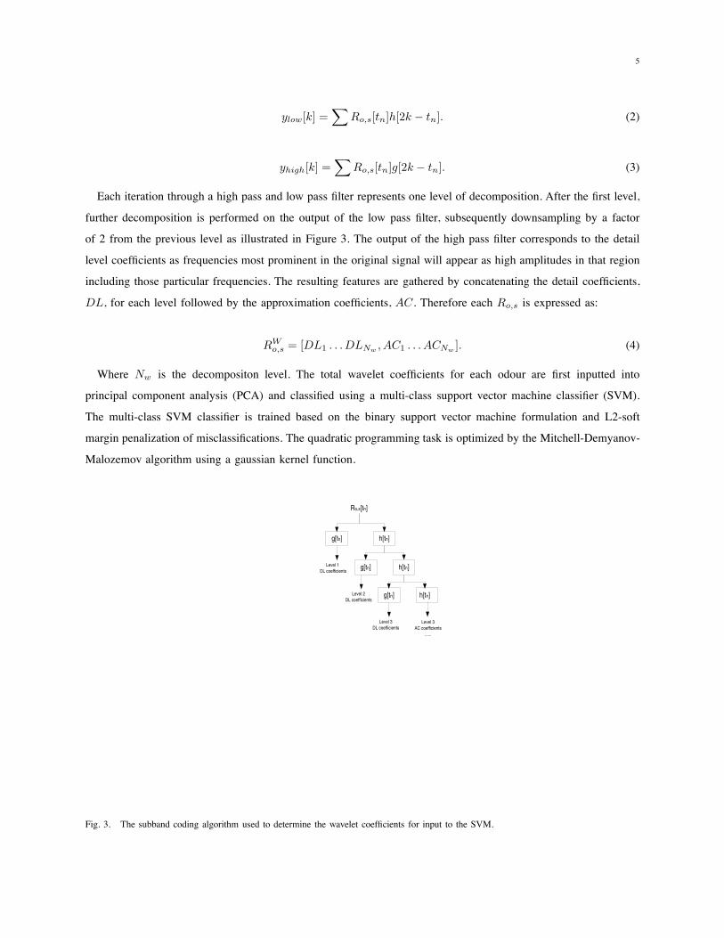
Each iteration through a high pass and low pass filter represents one level of decomposition. After the first level,

further decomposition is performed on the output of the low pass filter, subsequently downsampling by a factor

of 2 from the previous level as illustrated in Figure 3. The output of the high pass filter corresponds to the detail

level coefficients as frequencies most prominent in the original signal will appear as high amplitudes in that region

including those particular frequencies. The resulting features are gathered by concatenating the detail coefficients,

DL, for each level followed by the approximation coefficients, AC. Therefore each Ro,s is expressed as:

RWo,s = [DL1 . . .DLNw , AC1 . . . ACNw ]. (4)

Where Nw is the decompositon level. The total wavelet coefficients for each odour are first inputted into

principal component analysis (PCA) and classified using a multi-class support vector machine classifier (SVM).

The multi-class SVM classifier is trained based on the binary support vector machine formulation and L2-soft

margin penalization of misclassifications. The quadratic programming task is optimized by the Mitchell-Demyanov-

Malozemov algorithm using a gaussian kernel function.

Fig. 3. The subband coding algorithm used to determine the wavelet coefficients for input to the SVM.

6

0 5 10 15 20 25 30 35 40 45 502

2.5

3

3.5

4

4.5

5

time(s)

volta

ge(V

)

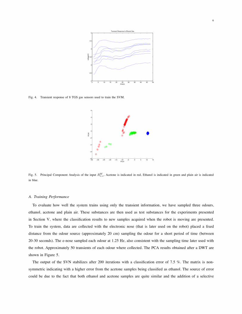
Transient Response to Ethanol Gas

Fig. 4. Transient response of 8 TGS gas sensors used to train the SVM.

−35 −30 −25 −20 −15 −10 −5 0 5 10 15−8

−6

−4

−2

0

2

4

6

111111111111111111111111111111111111111111111111111111111111

3333233332333333333333333233333333333

3333333

33

222222222222222

222222222222222222222222

2

2

2

222

PCA1

2

33

33

2

22

2

2

PCA2

Fig. 5. Principal Component Analysis of the input RWo,s, Acetone is indicated in red, Ethanol is indicated in green and plain air is indicated

in blue.

A. Training Performance

To evaluate how well the system trains using only the transient information, we have sampled three odours,

ethanol, acetone and plain air. These substances are then used as test substances for the experiments presented

in Section V, where the classification results to new samples acquired when the robot is moving are presented.

To train the system, data are collected with the electronic nose (that is later used on the robot) placed a fixed

distance from the odour source (approximately 20 cm) sampling the odour for a short period of time (between

20-30 seconds). The e-nose sampled each odour at 1.25 Hz, also consistent with the sampling time later used with

the robot. Approximately 50 transients of each odour where collected. The PCA results obtained after a DWT are

shown in Figure 5.

The output of the SVN stabilizes after 200 iterations with a classification error of 7.5 %. The matrix is non-

symmetric indicating with a higher error from the acetone samples being classified as ethanol. The source of error

could be due to the fact that both ethanol and acetone samples are quite similar and the addition of a selective

7

Fig. 6. Discretisation of the Gaussian weighting function onto the grid. Left side: For each grid cell within a cutoff radius R co (represented

by a circle) around the point of measurement !xt, the displacement !δ(i,j)t is calculated. The corresponding distances are indicated for the 13

affected cells by the vertical lines drawn in the upper part. The weights w(i,j)t are determined for all grid cells by applying a Gaussian function.

(σ = 1/3R co). Right side: An example of a completed gas distribution map representing a 3m x 4m area, the weights are indicated by shadings

of grey (dark shadings correspond to high weights). A second colour and inverse shading scheme is used for concentration values exceeding

80%. A dotted line indicates the path of the robot.

sensor could resolve the ambiguity (however, in this case a more symmetric confusion matrix would be generated).

Another and more likely possibility is that at certain concentration levels within specifc sample intervals, the transient

reactions of acetone generate a similar response to the those of ethanol. Table I.

TABLE I

CONFUSION MATRIX FOR CLASSIFICATION PERFORMANCE OF SVM.

Classifier

Substance Ethanol Acetone Air

Ethanol 35 0 0

Acetone 12 54 0

Air 0 0 60

III. GAS DISTRIBUTION MAPPING

To be able to visualize the distribution of a particular gaseous compound, the classification algorithm is integrated

with a gas concentration mapping (GDM) algorithm. Gas concentration mapping is a relatively new field in the area

of olfactory robots, with some progress made with both single and multiple robots [11], [8], [19]. The algorithm

applied here is based on the algorithm presented by [14] and further developped by the authors in [13].

Due to fundamental differences between range sensing with a laser scanner and gas sensing with metal oxide

sensors, traditional mapping techniques such as Bayesian estimation cannot be applied to the gas distribution

mapping problem in the same way as to estimate an occupancy grid map.

8

The main differences are, first, that the sensor readings do not allow to derive the instantaneous concentration

levels directly. Metal oxide gas sensors are known to recover slowly after the target gas is removed (15 to 70 seconds

[1]) and therefore perform temporal integration implicitly. Second, a snapshot of the gas distribution at a given

instant contains little information about the distribution at another time due to the chaotic nature of turbulent gas

transport. Turbulence generally dominates the dispersal of gas. As a consequence the instantaneous concentration

field of a target gas released from a small static source is a chaotic distribution of intermittent patches with peak

concentration values that are generally an order of magnitude higher compared to the time-averaged values [21].

Third, in contrast to a typical range-finder sensor, a single measurement from a gas sensor provides information

about a very small area because it represents only the reactions at the sensor’s surface. Another consequence of the

peculiarities of gas transport and gas sensing is that the gas sensor measurements do contain only little information

about the current sensor location with respect to the time-averaged gas distribution.

In order to estimate a grid map that represents the time-averaged relative concentration of a detected gas, we use

the kernel extrapolation gas distribution mapping method introduced by Lilienthal and Duckett [14]. The main idea

is to interpret the gas sensor measurements as noisy samples from a time-constant distribution. This implies that

the gas distribution in fact exhibits time-constant structures, an assumption that is often fulfilled in unventilated and

unpopulated indoor environments [24]. It is important to note that the noise is caused by the large fluctuations of

the instantaneous gas distribution while the electronic noise on individual gas sensor readings is negligible [9].

The kernel extrapolation gas distribution mapping method can cope to a certain degree with the temporal and

spatial integration of successive readings that metal-oxide gas sensors perform implicitly due to their slow response

and long recovery time [15]. In order to obtain a faithful representation of gas distribution despite the slow sensor

dynamics (“memory effect”), the robot’s path needs to fulfill the requirement that the directional component of the

distortion due to the memory effect is averaged out. This can be achieved by driving the robot through the same

coordinate from opposing directions.

The algorithm introduces the kernel width σ as a selectable parameter, corresponding to the size of the region of

extrapolation around each measurement. This parameter allows the user to decide between a faster or more accurate

map building process. Its value has to be set large enough to obtain sufficient coverage according to the path of the

robot. Conversely, this means that for a larger kernel width a faster convergence can be achieved while preserving

less detail of the gas distribution in the map. Consequently, the selected value of the kernel width σ represents a

trade-off between the need for sufficient coverage and the aim to preserve fine details of the mapped structures.

Parameter selection and the impact of sensor dynamics are discussed in more detail in [15].

Step-by-Step Explanation of Kernel Based Gas Distribution Mapping

The sensor readings are convolved using the univariate two dimensional Gaussian function

f("x) =1

2πσ2e−

!x2

2σ2 . (5)

Then, the following steps are performed:

9

Fig. 7. Overview of the method used to integrate the classification algorithm with the GDM and finally the occupancy map. The signal is passed

through a number of odour filters which identifies specific odour character using transient response. The identified signals are subsequently fed

into the GDM which generates an image representing the gas distribution. Each image is then overlayed onto the spatial information obtained

from the occupancy map.

• In the first step the normalised readings rt are determined from the raw sensor readings Rt as

rt =Rt ! Rmin

Rmax ! Rmin, (6)

using the minimum and maximum (Rmin, Rmax) value of a given sensor.

• Then, for each grid cell (i, j) within a cutoff radius Rco, around the point "xt where the measurement was

taken at time t, the displacement "δ (i,j)t from the grid cell’s centre "x (i,j) is calculated as

"δ (i,j)t = "x (i,j) ! "xt. (7)

• Now the weighting w(i,j)t for all the grid cells (i, j) is determined as

w(i,j)t =

f("δ (i,j)t ) : δ(i,j)

t " Rco

0 : δ(i,j)t > Rco

(8)

• Next, two temporary values maintained per grid cell are updated with this weighting: the total sum of the

weights

Mx : W (i,j)t =

t∑

t′

w(i,j)t′ , (9)

and the total sum of weighted readings

Mxzgas : WR(i,j)t =

t∑

t′

rt′w(i,j)t′ . (10)

10

Fig. 8. Results from an inspection of an indoor room. Left: shows the path taken from the robot overlayed on the occupancy map. Middle:

An example of the GDM obtained from an acetone source. Right: An example of the GDM obtained from an ethanol source. Source position

is indicated by a circle. Position of the maximum concentration is indicated by a cross.

TABLE II

CLASSIFICATION PERFORMANCE AND GDM PERFORMANCE IN THE INDOOR EXPERIMENTS.

Substance Trials Classification Performance Distance to Maximum (cm)

Ethanol9 92.4% ± 9.8% 5.67 ± 3.02

4 88.3% ± 12.0% 7.85 ± 2.02

Acetone13 96.2% ± 5.67% 9.55 ± 3.89

5 94% ± 4.8% 8.75 ± 2.68

• Finally, if the total sum of the weights W (i,j)t exceeds the threshold value Wmin, the value of the grid cell is

set to

c(i,j)t = WR(i,j)

t /W (i,j)t : W (i,j)

t # Wmin. (11)

An example that shows how a single reading is convolved onto a 5 $ 5 gridmap is given in Figure 6. First,

thirteen cells are found to have a distance of less than the cutoff radius from the point of measurement (Figure

6, left). These cells are indicated in the right side of Figure 6 by a surrounding strong border. The weightings for

these cells are then determined by evaluating the Gaussian function for the displacement values. In this example,

the cutoff radius was chosen to be three times the width σ. The weights are represented by shadings of grey. Darker

shadings indicate higher weights, which correspond to a stronger contribution of the measurement value rt in the

calculation of the average concentration value for a particular cell. As an example, a gas distribution map is shown

in Figure 6 (Right).

IV. COMBINATION OF THE MAPS

The GDM algorithm has been previously implemented with the assumption of homogenous gas sensing types and

the presence of a single odour source. Under these assumptions equation 6 can be used with Rt which normalizes

each of the sensor responses and correctly associates a shading based on the amplitude of the signal and the

position of the sensor with respect to the center of the robot. However, if a heterogenous sensing array is used, the

normalization of each sensor response will generate a misrepresentation of the concentration value needed for the

11

GDM. This is due to the fact that sensors of different types react differently to the same odourant. So a TGS 2600

selective to alcohols will provide a strong reaction with high signal amplitude while a sensor of type TGS 2602 will

provide little reaction at all. Therefore, in order to use the GDM algorithm as specified above, the original signal

is first classified, collecting all sensor responses associated to a specific odour (denoted as odour filtering). The

subsequent gas distribution map is then only evaluated for similar sensing types. Figure 7 summarizes the approach

used in this work to combine the sensor modalities in a singular map. The original signal is first processed through

the odour filters, for each trained odour. This is done by parsing the signal into transients, using a threshold to

determine the change in the sensor response. The transients are identified and the position (x,y) and rotation (θ)

of the robot corresponding to the signal response in the transient are stored. Signal responses between identified

transients are associated to the odour id of the previous transient.

After classification the signal is separated according to each sensor. Similar sensor types are then collected and

used in the GDM (e.g. all TGS 2600). Note that each sensor has a unique position on the robot with respect to the

robot center. The sensor position with respect to the robot, the signal response from the sensor and the corresponding

position of the robot in the environment are used as input to the GDM. The GDM then combines the information

from the sensors and this is done for each odour type.

Finally, in order to relate the gas distribution map to spatial information about the robot position and nearby

obstacles, a localization module based on adaptive Monte Carlo particle filter was used. In this work the map of the

environment is generated a priori using a Rao-Blackwellized particle filter to address the SLAM problem. The final

map is provided to the system and the localization module returns the position and rotation estimate of the robot as

it inspects the area. The position estimates are used as input to the GDM and the laser data information and map

are merged together with the output of the GDM and classification module. An alternative method to using a map

generated a priori is to consider the SLAM problem in conjunction with the GDM process. This issue has been

considered further in detail in [13], however, for the purpose of the experiments presented here and the validation

of the classification performance the map is presupposed to be given a priori.

V. EXPERIMENTAL RESULTS

A. Indoor Experiments

In the first experiments, the robot is placed in a 3m x 4m indoor room and performs a sweeping motion in the

room as shown in Figure 8 (Left). Two odour types were used as sources, ethanol and acetone. In each trial only

one of the odour types was present at a time and placed approximately in the center of the room, marked by the

square in the figure. Half of the collected experiments were performed autonomously by the robot, while the other

half were performed with a human operator guiding the robot with a joystick. The purpose of the experiments are

to evaluate to following: the performance of the classification algorithm to real data, the performance of the gas

distribution map and finally the flexibility of the system to be teleoperated with a human present in the room. Table

II summarizes the results from the experimental trials.

12

The classification performance is computed by testing the algorithm presented in Section II to new signals

collected by the robot. Only two odour filters are used, acetone and ethanol. Although a third odour filter for the

clean air could be included, it is obmitted for visualization of the GDM. This is because the coloring scheme used

in the GDM indicate regions of lower odour “concentration” by darker shading. These regions also correspond to

an absence of the specified odour (i.e. higher presence of clean air).

The performance criteria of the GDM are evaluated based on the proximity of the maximum odour concentration

and its correlation to the actual source position. It should be noted that using this measure is not always accurate as

air currents may cause the maximum concentration to drift from the odour source, as remarked by [17]. However,

in the absence of a true ground truth measure, this estimate has been adequate for the experiments. Furthermore, the

examination of whether this estimate changes with regards to a human operated sweep vs. an autonomous sweep

is indicative of the validity of the human operated investigation. In Figure 8 a typical sweep is shown for both

different gas source types, with σ = 25cm and considering only the response from the TGS 2600 sensors for the

map creation.

The classification performance is relatively stable throughout the different test runs and at varying distances from

the odour source. This can be attributed in part to the type of the environment and the type of odour sources being

used. Since the robot in all cases is moving relatively slowly to reduce the effect of the robot’s movements on the

gas distribution, an experimental sweep takes approximately 30 to 40 minutes. Furthermore, the high volatility of

the gas sources cause the gas molecules to quickly distribute in the indoor room.

B. Semi-Outdoor Experiments

Using the same sources, a second experiment was performed in a larger and less structured environment with

both sources present at the same time but seperated by a large distance to minimize the effect of mixing. In Figure

9 (Left) the laser scan of a large partially indoor environment located at Malaga University, Spain was used. This

environment is composed of four connecting corridors. The upper corridor is approximately 20 meters by 2.5 meters

and is partially outdoor corridor used as a passageway. It connects to the lower corridor which is located indoors

via two smaller corridors (right and left) in the figure. The odour source positions are indicated by a small circular

region. The ethanol is placed in the indoor lower corridor and the acetone in the upper corridor. The path of the

robot, this time guided by a human operator, is indicated in the right most figure.

The final gas distribution map is shown in Figure 10 (Left). To distinguish between the two different sources,

two different shading colors are used for concentration values exceeded 80% of the maximum signal amplitude.

The distance between the concentration maximum is 5.6 cm for the ethanol source and 48.2 cm for the acetone

source. It is expected that since the acetone source is placed in a partially outdoor environment, turbulent airflow

may have carried or displaced gaseous molecules from the source location causing not only the maximum measured

concentration to be far from the source location but also a much more dispersed plume to be present. For comparison,

in Figure 10 (Right), a gas distribution map is generated using the entire signal without consideration of the odour

classification but only averaging the signals from the same sensor type. The main difference here is that the spread

13

of the acetone gas is much more prominent especially in comparison to the ethanol source. This result is expected if

acetone signals generally produce a strong reaction for the TGS 2600 sensor. Therefore, by using the classification

algorithm as presented in the scheme Figure 7 the maximum concentration of each odour is equally represented in

the map as opposed to only capturing the maximum reaction of the entire signal. This facilitates the detection of

multiple odours despite a biased selectivity of the sensor.

Fig. 9. (Left) Occupancy Map of the long corridor experiment with source positions, acetone source is located in the upper corridor and the

ethanol source is located in the lower (indoor) corridor. (Right) Path of robot guided by the human user, a series of two passageways connect

the lower and upper corridor to each other.

Fig. 10. The gas distribution map of the corridor and the largest map made. (Left) The presence of the two sources is indicated using different

coloring schemes, green represents the ethanol and red represents the acetone source. Only concentrations exceeding 80% of the maximum for

each odour are displayed in color. (Right) No classification is performed and therefore only one color is used to represent the spread of the

odour. Without classification the Ethanol source is under represented.

Examining the classification performance is again another challenge given the presence of two odours and the

absence of knowledge about the particularities of odour mixtures and its effect on the response from the sensors. To

avoid mixing, the sources have been placed at a far distance from each other. The final classification performance is

14

TABLE III

CLASSIFICATION PERFORMANCE IN LONG CORRIDOR WITH TWO ODOUR SOURCES

Substance 5-20 cm 20-50 cm 50-100 cm 100-150 cm 150-250 cm 250-350 cm

Ethanol 100% 98.2% 98.2% 87.5% 85.5% 86.5%

Acetone 100 % 97.0 % 100 % 95.4 % 96.3% 93.2 %

presented in terms of the distance of the robot to the actual source position. Table III, summarizes the classification

performance and shows that as the distance from the source increases the classification performance degrades. If one

would test with the two sources closer together, the SVM would need to be trained on different possible mixtures

of the odours.

VI. CONCLUSION

In this work we presented a robotic system which combines techniques in static olfaction, and mobile robotics

to create a holistic representation of a gas distribution that includes classification and spatial information. The

experimental results show that the robot performs equally well when operated autonomously as when operated

by a human user. Experiments were performed with reasonable results in large and unmodified environments,

this combined with the importance of including classification information of an odour are significant contributions

towards real world applications for olfactory robots.

A number of remaining challenges are still worth noting. Firstly, classification of odour mixtures is still a

difficult problem particularly for systems which are not previously trained to detect the specific mixture. A better

understanding of the response from the gas sensors and in particular when used on a mobile robot is needed.

Another significant challenge is the problem of ground truth evaluation which although clearly present for the gas

distribution evaluation is also present for the classification problem. A possible direction for future work may be

to consider multiple robots working in the same environment, but using different techniques for measuring gas

distribution. A secondary alternative may be to combine information from different sensors, such as information

about how odours propagate around obstacles and wind information in order to verify the correlation to the gas

sensing results.

VII. ACKNOWLEDGMENTS

This work has been supported by the Swedish Research Council (Vetenskapsraadet). The authors would also like

to thank Jose Luis Blanco and Cipriano Galindo, University of Malaga for providing valuable support during the

experimental implementation.

REFERENCES

[1] K. J. Albert and N. S. Lewis, “Cross Reactive Chemical Sensor Arrays,” Chem. Rev., vol. 100, pp. 2595–2626, 2000.

[2] S. Badia, U. Bernardet, A. Guanella, P. Pyk, and P. Verschure, “A biologically based chemo-sensing uav for humanitarian demining,”

International Journal of Advanced Robotic Systems, vol. 4, no. 2, pp. 187–198, 2007.

15

[3] C. Distante, M. Leo, P. Siciliano, and K. Persaud, “On the study of feature extraction methods for an electronic nose,” Sensors and

Actuators B, vol. 87, pp. 274–288, 2002.

[4] ——, “Olfactory sensory system for odour-plume tracking and localization,” Sensors, vol. 1, pp. 418–423, 2003.

[5] T. Duckett, M. Axelsson, and A. Saffiotti, “Learning to locate an odour source with a mobile robot,” in Proceedings of the IEEE International

Conference on Robotics and Automation (ICRA’2001), Seoul, Korea, 2001.

[6] Figaro Gas Sensor: Technical Reference, 1992. http://www.figaro.com.

[7] R. Gutierrez-Osuna, A. Gutierrez-Galvez, and N. U. Powar, “Transient response analysis for temperature modulated chemoresistors,”

Sensors and Actuators B: Chemical B, vol. 93, no. 1-3, pp. 57–66, 2003.

[8] A. T. Hayes, A. Martinoli, and R. M. Goodman, “Distributed Odor Source Localization,” IEEE Sensors, vol. 2, no. 3, pp. 260–273, 2002.

[9] H. Ishida, A. Kobayashi, T. Nakamoto, and T. Moriizumi, “Three-Dimensional Odor Compass,” IEEE Transactions on Robotics and

Automation, vol. 15, no. 2, pp. 251–257, April 1999.

[10] H. Ishida, T. Nakamoto, and T. Moriizumi, “Remote sensing of gas/odor source location and concentration distribution using mobile

system,” Sensors and Actuators B, vol. 49, pp. 52–57, 1998.

[11] H. Ishida, T. Yamanaka, N. Kushida, T. Nakamoto, and T. Moriizumi, “Study of Real-Time Visualization of Gas/Odor Flow Images Using

Gas Sensor Array,” Sensors and Actuators B, vol. 65, pp. 14–16, 2000.

[12] A. Lilienthal and T. Duckett, “Creating gas concentration gridmaps with a mobile robot,” in Proceedings of the 2003 IEEE/RSJ International

Conference on Intelligent Robots and Systems (IROS 2003). IEEE Press, 2003.

[13] A. Lilienthal, A. Loutfi, J. Blanco, C. Galindo, and J. Gonzalez, “A rao-blackwellisation approach to gdm-slam - integrating slam and gas

distribution mapping,” in Proceedings of the 3rd European Conference on Mobile Robots (ECMR), 2007, p. To appear.

[14] A. J. Lilienthal and T. Duckett, “Creating Gas Concentration Gridmaps with a Mobile Robot,” in Proc. IEEE IROS, 2003, pp. 118–123.

[15] ——, “Building Gas Concentration Gridmaps with a Mobile Robot,” Robotics and Autonomous Systems, vol. 48, no. 1, pp. 3–16, August

2004.

[16] A. J. Lilienthal, A. Loutfi, and T. Duckett, “Airborne chemical sensing with mobile robots,” Sensors, vol. 6, pp. 1616–1678, October

2006. [Online]. Available: http://www.mdpi.org/sensors/papers/s6111616.pdf

[17] A. J. Lilienthal, H. Ulmer, H. Frohlich, F. Werner, and A. Zell, “Learning to detect proximity to a gas source with a mobile robot,” in

Proceedings of the IEEE/RSJ International Conference on Intelligent Robots and Systems (IROS), September 28 – October 2 2004, pp.

1444–1449.

[18] A. Loutfi, S. Coradeschi, L. Karlsson, and M. Broxvall, “Object recognition: A new application for smelling robots,” Robotics and

Autonomous Systems, vol. 52, pp. 272–289, 2005.

[19] L. Marques, A. Martins, and A. Almeida, “Environmental monitoring with mobile robots,” in Proceedings of the IEEE/RSJ International

Conference on Intelligent Robots and Systems (IROS), 2005, pp. 3624– 3629.

[20] L. Marques, U. Nunes, and A. de Almeida, “Olfaction-based mobile robot navigation,” Thin Solid Films, vol. 418, pp. 51–58, 2002.

[21] P. J. W. Roberts and D. R. Webster, “Turbulent Diffusion,” in Environmental Fluid Mechanics - Theories and Application, H. Shen,

A. Cheng, K.-H. Wang, M. Teng, and C. Liu, Eds. ASCE Press, Reston, Virginia, 2002.

[22] O. Rochel, D. Martinez, E. Hugues, and F. Sarry, “Stereo-olfaction with a sniffing neuromorphic robot using spiking neurons,” in

16th European Conference on Solid-State Transducers - EUROSENSORS, Prague, Czech Republic, Sep. 2002. [Online]. Available:

http://www.loria.fr/publications/2002/A02-R-139/A02-R-139.ps

[23] R. Russell, D. Thiel, and A. Mackay-Sim, “Sensing odour trails for mobile robot navigation,” in In IEEE Int. Conf. Robotics and Automation

(ICRA 1994), 1994, pp. 2672–2677.

[24] M. R. Wandel, A. J. Lilienthal, T. Duckett, U. Weimar, and A. Zell, “Gas Distribution in Unventilated Indoor Environments Inspected by

a Mobile Robot,” in Proc. IEEE ICAR, 2003, pp. 507–512.