Fuzziness and Uncertainty in Temporal Reasoning

Fuzziness and Uncertainty in Temporal Reasoning

Didier Dubois (Institut de Recherche en Informatique de Toulouse

Université Paul Sabatier, 118 route de Narbonne, 31062 Toulouse Cedex 4, France

[email protected])

Allel HadjAli (Institut de Recherche en Informatique de Toulouse


[email protected])

Henri Prade (Institut de Recherche en Informatique de Toulouse


prade @irit.fr)

Abstract: This paper proposes a general discussion of the handling of imprecise and uncertain information in temporal reasoning in the framework of fuzzy sets and possibility theory. The introduction of fuzzy features in temporal reasoning can be related to different issues. First, it can be motivated by the need of a gradual, linguistic-like description of temporal relations even in the face of complete information. An extension of Allen relational calculus is proposed, based on fuzzy comparators expressing linguistic tolerance. Fuzzy Allen relations are defined from a fuzzy partition made by three possible fuzzy relations between dates (approximately equal, clearly smaller, and clearly greater). Second, the handling of fuzzy or incomplete information leads to pervade classical Allen relations, and more generally fuzzy Allen relations, with uncertainty. The paper provides a detailed presentation of the calculus of fuzzy Allen relations (including the composition table of these relations). Moreover, the paper discusses the patterns for propagating uncertainty about (fuzzy) Allen relations in a possibilistic way. Keywords: Allen temporal relations, fuzzy relation, approximate reasoning, fuzzy interval, necessity measure, possibility theory Category: I.2.4

1 Introduction

Temporal information may be often perceived or expressed in a fuzzy way. However, temporal reasoning [Vila (1994)] and fuzzy set-based approximate reasoning [Bezdek et al. (1999)] have often been developed separately for about three decades. Indeed, there do not exist many studies about the handling of imprecise or uncertain information in temporal reasoning. Let us briefly mention a few exceptions. Dubois and Prade (1989) discuss approximate reasoning with fuzzy dates and fuzzy intervals

Journal of Universal Computer Science, vol. 9, no. 9 (2003), 1168-1194submitted: 10/2/03, accepted: 9/6/03, appeared: 28/9/03 © J.UCS

in the framework of possibility theory. Guesgen et al. (1994) introduce fuzzy Allen relations as fuzzy sets of ordinary Allen relations agreeing with a neighborhood structure. Fuzzy sets which play a key role in modeling flexible constraints, have been used in several constraint-based approaches to temporal reasoning. Qian and Lu (1989) propose several propagation strategies for handling networks of fuzzy temporal rules; Barro et al. (1994) propose a straightforward generalization of the notion of metric temporal constraint based on fuzzy sets and use possibility measures to check the consistency degree of a fuzzy temporal constraint network (see also [Vila and Godo (1994)] and [Wainer and Sandri (1998)]); Godo and Vila (1995) propose an approximate temporal logic based on the embedding into the logical language of fuzzy temporal constraints between pairs of time points. The inference system is based on specific rules dealing with the temporal constraints and a fuzzy modus ponens rule handling certainty qualified statements (see also the recent work of [Cárdenas et al. (2001)]). Dubois et al. (1991) have proposed a possibilistic temporal logic where each classical logic formula is associated with the fuzzy set of time points where the formula is certainly true to some extent. More recently, the fuzzy representation and processing of imprecise temporal knowledge has been applied to Petri net-based models of discrete event systems for the purpose of simulation and fault diagnosis [Cardoso and Camargo (1999)] (see also [Cardoso et al. (1999)] for Petri nets in the framework of possibility theory). Let us also mention the work done by Freksa (1992) who proposes a generalization of Allen's interval-based approach to temporal reasoning, based on semi-intervals, for processing coarse and incomplete information.

The introduction of fuzzy features in temporal reasoning can be done in different manners, depending on the representation level which is chosen, and according to the problem at hand. This may be motivated by the handling of fuzzy or incomplete information, or by the need for an approximate or gradual description of temporal relations even in the face of complete information. In the following we provide a general discussion of these representational issues in the framework of fuzzy set and possibility theory (already used in most of the above-mentioned references).

Time is usually represented in terms of dates, or in terms of intervals. Thinking in terms of dates, and assuming a linear time scale, we can compare dates in terms of the three relations >, = and <. Considering intervals, the thirteen qualitative relations first extensively discussed by [Allen (1983)], describe the possible relative positions of two intervals w.r.t. each other. These relations can be defined in terms of the three previous relations applied to the bounds of the intervals. Temporal reasoning then amounts to computing the transitive closure of this set of relations between intervals.

When dealing with fuzziness and uncertainty in approximate reasoning, two situations have to be carefully distinguished. On the one hand, one may have to evaluate fuzzy statements (by graded truth values) in the presence of complete information. On the other hand, one may have to compute the uncertainty associated with non-fuzzy statements (which are thus true or false) when the available information is imprecise, uncertain or fuzzy. Obviously, these two extreme cases can be combined if we are interested in the evaluation of fuzzy statements in presence of incomplete information.

These two extreme cases can be encountered as well with temporal information: i) The information about dates and relative positions of intervals is complete, but for some reason we are not interested in describing it in precise terms. For instance, we want to speak in terms of approximate equality, or proximity, rather than in terms of

1169Dubois D., HadjAli A., Prade H.: Fuzziness and Uncertainty ...

precise equality in order to avoid brutal discontinuities between the cases of values that are perfectly equal and of values that are very close to each other. This is more generally related to the issue of interfacing a numerical continuum with a finite number of categories, where the use of fuzzy categories allows for smooth transitions between them. The concern of assessing the closeness of two dates may be also related to the general issue of expressing fuzzy information about duration in temporal reasoning. ii) The available information is pervaded with imprecision, vagueness or uncertainty. This may cover slightly different situations: • relations between dates or intervals are known with precision and certainty, but some dates may be imprecisely located (the date belongs to some interval), fuzzily located (the more or less possible values of the date are restricted by a fuzzy set acting as an elastic constraint), or dates are pervaded with uncertainty (which means that we are not even sure that the date is in some (fuzzy) range, and there is a possibility that its value is unknown). • our knowledge about the three possible relations between some dates, or the thirteen relations between some intervals are pervaded with imprecision, uncertainty or vagueness.

This paper discusses these representational issues in a rather systematic way. It substantially develops the contents of a recent working note [Dubois and Prade, 2002]. Especially, the paper uses a set of three fuzzy relations between dates, modeling the ideas of being approximately equal, clearly before, or clearly after, which make a fuzzy partition of the temporal axis. This fuzzy partition is characterized by a unique parameter. In particular, using these three relations, the computation of the composition table of the thirteen fuzzified extensions of Allen relations is established. In Section 3, fuzzy counterparts to Allen relations are provided where each temporal relation is associated with a fuzzy parameter. Reasoning about such temporal information is discussed. Section 4 deals with Allen relations, or their fuzzified versions, when the available knowledge is pervaded with uncertainty. Deductive patterns of reasoning involving fuzzy or uncertain temporal knowledge are then established. First a background section recalls Allen’s relations as well as results about the composition of fuzzy relations modeling approximate equalities or comparing the magnitude of values.

2 Background

The purpose of this background is twofold. First the possible relations describing the relative locations of two intervals are restated. Then, fuzzy inference rules involving fuzzy approximate equalities and graded inequalities are established.

In the following, we denote dates by italic lower case letters a, b, c,..., intervals by italic capital letters A, B, C,...and fuzzy sets by ordinary capital letters.

1170 Dubois D., HadjAli A., Prade H.: Fuzziness and Uncertainty ...

2.1 Allen Temporal Relations

Allen (1983) has proposed a set of basic mutually exclusive primitive relations that may hold between temporal intervals. These relations between events are usually denoted by before ( ), after ( ), meets (m), met by (mi), overlaps (o), overlapped by (oi), during (d), contains (di), starts (s), started by (si), finishes (f), finished by (fi), and equals (≡). Their meanings are pictured in Table 1.

Relation Converse Pictorial Example Endpoints Relations

A �B B A A m B B mi A A o B B oi A A s B B si A A d B B di A A f B B fi A A ≡ B B ≡ A

b > a’

a’ = b

b > a ∧ a’ > b ∧ b’ > a’

a = b ∧ b’ > a’

a > b ∧ b’ > a’

a > b ∧ b’ = a’

a = b ∧ a’ = b’

Table 1: The thirteen qualitative relations between two intervals

It is clear that the above relations can be defined from the three binary relations <,

=, and > applied to the bounds of two intervals to be located w.r.t each other. For instance, assuming that for any interval A, the smallest endpoint is denoted by a and the greatest one by a’ then, the assertion A overlaps B corresponds to (b > a) ∧ (a’ > b) ∧ (b’ > a’) as shown in Table 1. Only a subset of relations between the endpoints of intervals we consider is sufficient for fully characterizing their qualitative relations due to two domain-inherent conditions: (i) the least points of intervals take place before the greatest endpoints and (ii) the relations <, =, > are transitive.

Allen (1983) has provided a set of axioms describing the composition of the thirteen relations, together with an inference procedure. For instance, A before B and B before C ⇒ A before C, A meets B and B during C ⇒ (A overlaps C ∨ A during C ∨ A starts C).

B

B

B

B

A

A

B A

A

B

A

A

A

B


The last example shows that Allen was forced to introduce disjunctions of primitive relations for dealing with uncertainty about the relationship, even for the composition of two primitive relations.

Let us note that a generalization of Allen’s interval-based approach, based on semi-intervals, has been proposed by Freksa (1992) for reasoning with incomplete knowledge, specifically with coarse knowledge about temporal relationships. The notion of "conceptual neighborhood" is central in this approach. The following definitions have been introduced by him:

Definition 1. Two relations between pairs of events are (conceptual) neighbors, if they can be directly transformed into one another by continuously deforming in one way (i.e. either shortening, or lengthening, or moving) one of the events (in a topological sense). Examples. The relations before ( ) and meets (m) are conceptual neighbors. By contrast, the relation before ( ��and overlaps (o) are not conceptual neighbors. Definition 2. A set of relations between pairs of events forms a (conceptual) neighborhood if its elements are path-connected through ’conceptual neighbor’ relations. Examples. The relations before ( ), meets (m) and overlaps (o) form a (conceptual) neighborhood. By contrast, the relations before ( ) and overlaps (o) do not form a conceptual neighborhood.

According to the above definition of the conceptual neighborhood, Freksa makes an arrangement of the thirteen mutually exclusive relations between events in such a way that conceptually neighboring relations become neighbors (see Figure 1.a). Depending on the types of deformation of events and their relations, we obtain different neighborhood structures. For instance, if we fix three of the four semi-intervals of two events and allow the fourth to vary, we obtain the A-neighbor relation (see Figure 1.b). For more details about the two other neighborhood structures, see [Freksa (1992)].


(a) (b) Figure 1: Allen’s thirteen primitive relations arranged according to their conceptual

neighborhood.

2.2 Fuzzy Absolute Comparators

The representation of fuzzy comparators expressed in terms of difference of values is discussed. Then the composition of fuzzy relations modeling approximate equalities, or graded inequalities, is recalled, and inference rules involving such fuzzy parameterized relations are then established. Let us first recall the concept of fuzzy set.

2.2.1 Fuzzy Set

The concept of a fuzzy set has been introduced by Zadeh (1965) to deal with the representation of classes whose boundaries are ill-defined, or flexible, by means of characteristic functions taking values in the interval [0, 1]. A fuzzy set F in referential U is thus characterized by a membership function µF: U → [0, 1], where the value µF(u) represents the "grade of membership" of u in F. In particular, µF(u) = 1 reflects full membership of u in F, while µF(u) = 0 expresses absolute non-membership in F. Usual sets can be viewed as special cases of fuzzy sets where only full membership and absolute non-membership are allowed (they are called crisp sets, or Boolean sets). When 0 < µF(u) < 1, one speaks of partial membership.

Two crisp sets are of particular interest when defining a fuzzy set F, the core (i.e. {u, µF(u) = 1}) and the support (i.e. {u, µF(u) > 0}). A trapezoidal membership function can be encoded by a 4-tuple(a, b, α, β), where the intervals [a, b] and [a−α, b+β] represent the core and the support of the fuzzy set respectively. See Figure 2.

m

d

s

o

f

=

mi

oi

fi

di

si

m

d

s

o

f

=

mi

oi

fi

di

si


Figure 2: Trapezoidal membership function Fuzzy quantity. A fuzzy quantity Q is any fuzzy set of the real line 3, assumed to be normalized (i.e. ∃ u, µQ(u) = 1). Fuzzy interval. A fuzzy interval M is a fuzzy quantity with a quasi-concave membership function, i.e., a convex fuzzy set of the real line 3 which obeys the following constraint: ∀ u, u', ∀ u" ∈ [u, u'], µM(u") ≥ min(µM(u), µM(u')). The fuzzy set pictured in Figure 2 represents a trapezoidal fuzzy interval. Fuzzy arithmetic operations. Let M = (a, b, α, β) and N = (a', b', α', β') be two fuzzy intervals. Extended sum ⊕ and extended subtraction − between fuzzy intervals can be defined in the framework of possibility theory [Dubois and Prade (1988)]. With the above trapezoidal representation, it amounts to the following computation: M ⊕ N = (a + a', b + b', α + α', β + β'), M − N = (a − b', b − a', α + β', β +α'). For more details about all these notions, the reader can consult Chapters 1 and 10 of [Dubois and Prade 2000].

2.2.2 Approximate Equalities and Graded Inequalities

An approximate equality between two values, here representing dates, modeled by a fuzzy relation E with membership function µE (E stands for "equal"), can be based on a distance such as the absolute value of the difference. Namely, µE(x,y) = µL(|x − y|), where L is a fuzzy set modeling the fuzzy amount of discrepancy between values regarded as approximately equal. For simplicity, fuzzy sets and fuzzy relations are assumed to be defined on the real line. But we could restrict ourselves to integer or to rational values if necessary. Approximate equality is represented by

µF(u)

U b a

1

b+β a−α


∀x, y ∈3,

( )⎪⎪

⎩

⎪⎪

⎨

⎧

ε−−ε+δ

ε+δ>δ≤

=⎟⎟⎠

⎞⎜⎜⎝

⎛⎟⎟⎠

⎞⎜⎜⎝

⎛ε

−−ε+δ=−=µ

otherwise yx

y-x if 0

y-x if 1

yx

,1 min,0 max)yx(µy,x LE

(1)

where δ and ε are respectively positive and strictly positive parameters which affect the approximate equality. Here L is a fuzzy set centered in 0, i.e. µL(d) = µL(−d) in order to have E symmetrical: µE(x, y) = µE(y, x). See Figure 3. Classical equality is

recovered for δ = 0 and ε → 0. Then the approximate equality of quantities a and b (in the sense of E) can be

written under the form a − b ∈ L ⇔ b − a ∈ L ⇔ a E(L) b

with the following intended meaning: the possible values of the difference a − b are restricted by the fuzzy set L. In particular a E(0) b means a = b. Note that we may also think of modeling an approximate equality in terms of the closeness of the ratio x/y to 1. This is the basis of the calculus of fuzzy relative orders of magnitude, expressed in terms of closeness and negligibility relations, which has been developed in [HadjAli et al. (2003)]. However, a difference-based view of approximate equality appears to more suitable for temporal modeling where the difference between dates make sense, but not their ratio usually.

1

−δ−ε −δ 0 δ δ+ε λ λ+ρ

L

K

λ−δ−ε λ+ρ−δ

x-y

L K⊕

Figure 3: Modeling "approximate equality" and "graded strict inequality".

Similarly, a more or less strong inequality can be modeled by a fuzzy relation G

(G stands for "greater"), of the form µG(x,y) = µK(x − y).


In the following, we take ∀x, y ∈3,

( )

otherwise. yx

yx if 0

yx if 1

yx

,1 min,0 max)yx(y,x KG

⎪⎪

⎩

⎪⎪

⎨

⎧

ρλ−−

λ+≤ρ+λ+>

=⎟⎟⎠

⎞⎜⎜⎝

⎛⎟⎟⎠

⎞⎜⎜⎝

⎛ρ

λ−−=−µ=µ

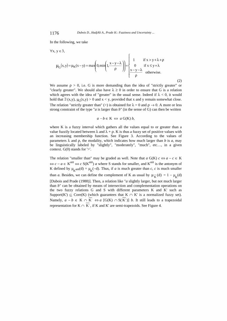
(2) We assume ρ > 0, i.e. G is more demanding than the idea of "strictly greater" or "clearly greater". We should also have λ ≥ 0 in order to ensure that G is a relation which agrees with the idea of "greater" in the usual sense. Indeed if λ < 0, it would hold that ∃ (x,y), µG(x,y) > 0 and x < y, provided that x and y remain somewhat close.

The relation "strictly greater than" (>) is obtained for λ = 0 and ρ → 0. A more or less strong constraint of the type "a is larger than b" (in the sense of G) can then be written

a − b ∈ K ⇔ a G(K) b,

where K is a fuzzy interval which gathers all the values equal to or greater than a value fuzzily located between λ and λ + ρ. K is thus a fuzzy set of positive values with an increasing membership function. See Figure 3. According to the values of parameters λ and ρ, the modality, which indicates how much larger than b is a, may be linguistically labeled by "slightly", "moderately", "much", etc…, in a given context. G(0) stands for '>'. The relation "smaller than" may be graded as well. Note that a G(K) c ⇔ a − c ∈ K

⇔ c − a ∈ Kant ⇔ c S(Kant) a where S stands for smaller, and Kant is the antonym of K defined by µ

Kant(d) = µK

(−d). Thus, if a is much greater than c, c is much smaller

than a. Besides, we can define the complement of K as usual by )d(Kµ = 1 − µK

(d)

[Dubois and Prade (1988)]. Then, a relation like "a slightly larger, but not much larger than b" can be obtained by means of intersection and complementation operations on the two fuzzy relations G and S with different parameters K and K' such as Support(K') ⊆ Core(K) (which guarantees that K ∩ K' is a normalized fuzzy set).

Namely, a − b ∈ K ∩ ’K ⇔ a [G(K) ∩ S( ’K )] b. It still leads to a trapezoidal

representation for K ∩ ’K , if K and K' are semi-trapezoids. See Figure 4.


’K

0

K

x-y

’K ant

K’

Figure 4

However note that ant’K is no longer in such a case the parameter of a fuzzy relation

G agreeing with the idea of "strictly greater than", since ant’K includes negative

values (although somewhat close to 0).

2.2.3 Composition of Fuzzy Relations and Fuzzy Intervals

The composition G(K)°E(L) of two fuzzy relations G(K) and E(L) is defined by

∀ x ∈ X, ∀ z ∈ Z, µG(K)°E(L) (x,z) = supy ∈Y min(µG(x, y), µE(y, z))

= supy ∈Y min(µK(x − y), µL(y − z)) = sups,t: x−z = s+t min(µK(s), µL(t))

= µK⊕L(x − z),

where we recognize the expression of the extended sum ⊕ of fuzzy sets K and L. In

Figure 3, L = (–δ, δ, ε, ε), Κ = (λ + ρ, +∞, ρ, +∞) and K ⊕ L = (λ + ρ – δ, +∞,

ρ + ε, +∞).

If we know for instance that "a is approximately equal to b" (i.e. a E(L) b ) and that "b is much greater than c" (i.e. b G(K) c ), we can deduce that

a − c ∈ K ⊕ L ⇔ a G(K ⊕ L) c,

using the above composition formula. This result is represented in Figure 3 where the relations E(L) and G(K) are used. We see that it is certain that a > c + λ − (δ + ε) and that the value of the difference a − c belongs to L ⊕ K to degree 1 as soon as a ≥ c + λ + ρ − δ. Then, depending on the respective values of the parameters, a is still greater than c (but may be not as much as b with respect to c) (if λ − δ − ε > 0), or there is a non-zero possibility that a is slightly smaller than c (if λ + ρ − δ > 0), although it is more possible that a be larger than c.


2.2.4 Fuzzy Parameterized Inference Rules

Taking advantage of the fact that the composition of the fuzzy relations E(L) and G(K) reduces to simple arithmetic operations on the fuzzy parameters K and L underlying the semantics of E and G, fuzzily parameterized inference rules can be obtained.

Then, the following set of inference rules describing the behaviors of the fuzzy comparators E and G have been established in [Dubois et al. (2001)]:

• Basic properties of the fuzzy comparators E and G

R1 : a ≤ c ≤ b and a E(L) b ⇒ a E(L) c Convexity R2 : a E(L) b ⇔ b E(L) a Symmetry R3 : a E(L) b ⇔ a+c E(L) b+c E-Summation invariance R4 : a G(K) b ⇔ a+c G(K) b+c G-Summation invariance

• Closure rules

R5 : a E(L) b and b E(L’) c ⇒ a E(L⊕L’) c E-Transitivity R6 : a G(K) b and b G(K’) c ⇒ a G(K⊕K’) c G-Transitivity R7 : a E(L) b and b G(K) c ⇒ a G(K⊕L) c E-G-Composition

Note that rule R7 corresponds to the above example. Rule R5 expresses a

weakening of the transitivity property for approximate equalities: a may be not close to c in as much a is to b and b to c. On the contrary, R6 expresses a strengthening: a is much greater than c to a larger extent than a w.r.t. b, or b w.r.t. c. Thus, rules R1 to R7 enable us to formally compute the fuzzy parameters underlying the relations by means of an inference process, and then to interpret them.

From the above basic rules, other noticeable ones can be established:

• Summation stability

R8 : a E(L) b and c E(L’) d ⇒ a+c E(L⊕L’) b+d R9 : a E(L) b and c G(K) d ⇒ a+c G(L⊕K) b+d R10 : a G(K) b and c G(K’) d ⇒ a+c G(K⊕K’) b+d

Indeed, let us take the example of R8. Applying R3 yields a E(L) b ⇒ a+c E(L)

b+c and c E(L’) d ⇒ b+c E(L’) b+d, then by R5 we prove R8. It can be shown that in fact R8 is equivalent to R5 since R8 entails R5 (letting b = c in R8 and applying R3). Now, since a > b is equivalent to a G(0) b where K = 0 in the case where λ = 0 and ρ → 0 in (2). Then, the following intuitive properties of the fuzzy relation G can as well be derived using rule R6 (since K ⊕ 0 = K):

R11 : a > b and b G(K) c ⇒ a G(K) c, R12 : a G(K) b and b > c ⇒ a G(K) c,

Other rules can be established such as:

R13: a+b G(K) c+d and c E(L) a ⇒ b G(K⊕L) d, (using R3 two times and R7)


R14 : a+b E(L) c and c G(K) a ⇒ b G(L⊕K) 0. (using R9 and R4) Other rules involving duration could be derived as well. For instance, if a G(K) b

and b − c ∈ D then a G(K ⊕ D) c, where D represents the fuzzy information about the time spent between b and c.

3 Fuzzy Allen Relations

This section discusses an extension of Allen relations based on approximate equality and graded strict inequality relations defined from associated fuzzy parameters. Using inference rules established in Section 2.2.4, it is shown that the composition of classical Allen relations can be easily extended in practice by augmenting the classical calculus with the arithmetic manipulation of fuzzy parameters. The section ends with a brief outline of another possible approach based on possibilistic mathematical morphology notions.

3.1 Modeling

Using the fuzzy parameterized comparators E(L) and G(K), we can define fuzzy counterparts of Allen relations. The idea is that the relations which can hold between the endpoints of the intervals we consider may not be described in precise terms. For instance, we want to speak in terms of approximate equality (in the sense of E) rather in terms of precise equality in order to not introduce a brutal discontinuity between the case of a "perfect" meet relation and the case of a before relation when the upper bound of the first interval is close to the lower bound of the second interval.

Then, in approximate terms, only two distinct relations may hold between two dates a and b. Indeed, a date a can be "approximately equal" to a date b in the sense of E(L), or a can be "clearly different from" b in the sense of not E(L). This last relation corresponds to "much larger" in the sense of G(K) or "much smaller" in the sense of S(Kant). Then, the fuzzy parameters L, K and Kant are elements of a fuzzy partition (as shown in Figure 5) in the sense that ∀ d ∈ 3, µ

K(d) + µ

Kant(d) + µL(d) = 1.

K and Kant are obtained from L by fuzzy complementation. This makes a fuzzy partition since K ∪ Kant ∪ L = 3, and Kant ∩ L = ∅, K ∩ L = ∅ and K ∩ Kant = ∅, using the following union and intersection operators µ

F∪G(d) = min (1, µ

F(d) + µ

G(d))

and µF∩G

(d) = max (0, µF(d) + µ

G(d) − 1).


1

−δ−ρ −δ 0 δ δ+ρ

L K

x-y

Kant

Figure 5: Modeling "at least approximately equal" and "clearly different and greater (or smaller)".

Each parameter can be obtained from one another as follows:

) ,0[LK ∞+∩= which is denoted cL+ ,

]0 ,(LK ant −∞∩= which is denoted cL− .

Conversely L can be recovered from K as

antKKL ∪= which is denoted Kc. For trapezoidal representations, it means

If K = (γ, +∞, ρ, +∞) then Kc = (−γ+ρ, γ−ρ, ρ, ρ),

If L = (−δ, δ, ρ, ρ) then cL+ = (δ+ρ, +∞, ρ, +∞) and cL− = (−∞,−δ−ρ, +∞, ρ).

Thus having interrelated L, K and Kant enables us to have a unique parameter underlying these relations. This is what is assumed in the definition of the forthcoming fuzzy Allen relations. Thus it appears that E(L), G(K) and S(Kant) with L and K inter-defined as explained above, are fuzzy counterparts to the classical relations =, >, and < in the crisp case. Indeed, they define a fuzzy partition. Remark: It is possible to define counterparts of the relations ’≥’ and ’≤’ as respectively

the union of E(L) and G( cL+ ), namely GE(L) = E(L) ∪ G( cL+ ), and SE(L) as the

union of E(L) and S( cL− ), namely SE(L) = E(L) ∪ S( cL− ). Then it can be checked

that E(L) = SE(L) ∩ GE(L), using the above intersection. GE(L) and SE(L) behave as genuine extensions of ≥ and ≤. Indeed, it can be shown that a GE(L1) b and b GE(L2) a ⇒ a E(L1 ∪ L2) b where union on fuzzy parameters is defined using max operation. New inference rules involving these non strict graded inequality relations can be proved, e.g., the following ones that can be proved using a counterpart of R13 for GE and the above rule: a E(L) b and b+c GE(L1) a+d and d GE(L2) c ⇒ c E((L⊕ L1) ∪ L2) d.


Let A = [a, a’] and B = [b, b’] be two time intervals (it is assumed that all the considered intervals [a, a’] are such that a < a’). The fuzzy Allen relations can be now defined as shown in Table 2.

Fuzzy Allen Relation

Definition

Label

Label of Converse

A fuzz-before(L) B

B fuzz-after(L) A

b G( cL+ ) a’

fb(L)

fa(L)

A fuzz-meets(L) B

B fuzz-met by(L) A

a’ E(L) b

fm(L)

fmi(L)

A fuzz-overlaps(L) B

B fuzz-overlapped by(L) A

b G( cL+ ) a ∧ a’ G( cL+ ) b ∧

b’ G( cL+ ) a’

fo(L)

foi(L)

A fuzz-during(L) B

B fuzz-contains(L) A

a G( cL+ ) b ∧ b’ G( cL+ ) a’

fd(L)

fdi(L)

A fuzz-starts(L) B

B fuzz-started by(L) A

a E(L) b ∧ b’ G( cL+ ) a’

fs(L)

fsi(L)

A fuzz-finishes(L) B

B fuzz-finished by(L) A

a’ E(L) b’ ∧ a G( cL+ ) b

ff(L)

ffi(L)

A fuzz-equals(L) B

B fuzz-equals(L) A

a E(L) b ∧ b’ E(L) a’

fe(L)

fe(L)

Table 2: Fuzzy Allen Relations

Example: Assume that A = [a, a’] = [0, 5.6], B = [b, b’] = [6, 9], and C = [c, c’] = [9.6,

12] are time intervals. Let L = (−0.4, 0.4, 0.1, 0.1) (resp. K = cL+ = (0.5, +∝, 0.1, +∝))

be the fuzzy parameter underlying the semantics of an approximate equality E (resp. the associated fuzzy relation "clearly greater" G). See Figure 3. Since a’ E(L) b and c G(K) b’ then, the following fuzzy Allen relations hold :

A fuzz-meets(L) B, B fuzz-before(K) C. Here we start from absolute temporal knowledge and relative knowledge is derived. It

is possible to compute to what extent the above relations (respectively µE(L)(a’, b) and µG(K)(c, b') which are 1 here) are valid.

As we can see the introduced fuzzy Allen relations are of three types: i) relations which are defined only on the basis of the fuzzy inequality G, i.e. relations fb, fo, fd and their converses ; ii) relations which are defined both on the basis of the


approximate equality E and the fuzzy inequality G, i.e. relations fs, ff and their converses ; iii) relations which are defined only on the basis of the approximate equality E, i.e. relations fm, fe and their converses.

Guesgen et al. (1994) have proposed another modeling of fuzzy Allen relations. They define a fuzzy Allen relation as a fuzzy set of ordinary Allen relations, the membership grades being assessed in agreement with a neighborhood system between the relations (this notion of neighboring relations is the one introduced in [Section 2.1]). In the modeling proposed above, a fuzzy Allen relation also covers several situations corresponding to different ordinary Allen relations; for instance, fuzz-meets(L) covers the ordinary "meet" situation as well as situations as "slightly before" or "slight overlap". However here, the fuzzy parameter L controls to what extent we can shift from the ordinary "meet" situation, and provides a basis for the semantics of what "slightly" means in the above expressions. In the same way, we can see that fuzz-equals(L) can cover the ordinary situation expressed by "slightly contains" or "slightly during".

3.2 Reasoning Based on Fuzzy Allen Relations

As usual, we can reason on the basis of the established fuzzy Allen relations by computing the transitive closure of the fuzzy temporal relations using the inference rules given in [Section 2.2.4]. Let us first introduce some notations to be used in the forthcoming composition table. Let rp and rq be two relations among the thirteen fuzzy relations presented in Table 2. We denote by <rp..rq> the conceptual A-neighborhood (in the sense introduced in [Section 2.1]) that starts with the relation rp and finishes with the relation rq. The disjunctive set <rp..rq> contains the conceptual neighbor relations which form the shortest path between rp and rq. For instance, <fb..fd> contains {fb, fm, fo, fs, fd} and <fs..fsi> contains {fs, fe, fsi}.

Let us show on some examples how the axioms describing the transitivity behavior of the fuzzy Allen relations can be established (where A = [a, a’] denotes a time interval): i) Assume that we know that A fb(L1) B and B fb(L2) C, the temporal relation between A and C can be obtained as follows:

A fb(L1) B ⇔ b G( c1 )L( + ) a’,

B fb(L2) C ⇔ c G( c2 )L( + ) b’.

Now by applying rule R11 on b G( c1 )L( + ) a’, we obtain b’ G( c

1 )L( + ) a’ since b’ > b.

The transitivity rule R6 applied on c G( c2 )L( + ) b’ and b’ G( c

1 )L( + ) a’, implies that c

G( c2 )L( + ⊕ c

1 )L( + ) a’. This means that A fb(L2

⊕ L1) C since c2 )L( + ⊕ c

1 )L( + = c

21 )LL( +⊕ .

ii) Assume now that A fb(L1) B and B fmi(L2) C. Using the definitions of fb(L1) and fmi(L2), we have:


A fb(L1) B ⇔ b G( c1 )L( + ) a’,

B fmi(L2) C ⇔ b E(L2) c’ ⇔ c’ E(L2) b (due to rule R2).

By applying rule R7 on c’ E(L2) b and b G( c1 )L( + ) a’, we deduce

c’ G(L2 ⊕ c1 )L( + ) a’ (which will be denoted by H3). Now according to the location of

the date c with respect to dates a and a’, several mutually exclusive primitive relations may hold between the time intervals A and C. Let H1 (resp. H2), H’1 (resp. H’2), H1’’ and (resp. H’’2) denote the relations c > a (resp. c > a’), c = a (resp. c = a’) and c < a (resp. c < a’) respectively. Then, the different primitive relations that could hold between A and C are as follows:

fb = H2 (which means that fb only requires hypothesis H2) fm = H’2

fo = H1 ∧ H"2 ∧ H3 (which means that fo requires simultaneously hypotheses H1, H"2 and H3)

fs = H’1 ∧ H3 fd = H"1 ∧ H3

In a condensed form, the relation between A and C writes <fb..fd> corresponding to the disjunction of the atomic relations fb, fm, fo, fs and fd. Now, the fuzzy interval that should be associated to relation <fb..fd> can be computed as follows. The relations fb and fm can also be expressed as H1 ∧ H2 ∧ H3 and H1 ∧ H’2 ∧ H3 respectively (since H1 and H3 implicitly hold in these cases). The disjunction fb ∨ fm ∨ fo reduces to H1 ∧ H3 since H2∨ H’2∨ H"2 = T (where T is a tautology). Then, (fb ∨ fm ∨ fo) ∨ fs ∨ fd reduces as well to H3 since H1∨ H’1∨ H"1 = T. This means that the fuzzy temporal relation between A and C holds in the sense of the fuzzy set underlying the relation G that holds between the dates c’ and a’. Then we conclude that A <fb..fd>(L1) C with L1 =

[L1 ⊕ c2 )L( + ]c

iii) Assume now that A fs(L1) B and B fsi(L2) C. According to the definitions of fs(L1) and fsi(L2), the following two equivalences hold:

A fs(L1) B ⇔ a E(L1) b ∧ b’ G( c1 )L( + ) a’,

B fsi(L2) C ⇔ b E(L2) c ∧ b’ G( c2 )L( + ) c’.

The transitivity rule R5 applied to a E(L1) b and b E(L2) c enables to deduce a E(L1 ⊕ L2) c (which will be denoted by H1). Then, the atomic relations which could hold between A and C are: fs = H1 ∧ H3 (H3 stands for c’ > a’)

fe = H1 ∧ H’3 (H’3 stands for c’ = a’)

fsi = H1 ∧ H"3 (H"3 stands for c’ < a’)

In the similar way as above, we can also show that the disjunction fs ∨ fe ∨ fsi reduces to H1. This means that A <fs..fsi>(L1 ⊕ L2) C. iv) Assume now that A fs(L1) B and B ff(L2) C. Now the definitions of fs(L1) and ff(L2) enable us to write:


A fs(L1) B ⇔ a E(L1) b ∧ b’ G( c1 )L( + ) a’,

B ff(L2) C ⇔ b G( c2 )L( + ) c ∧ b’ E(L2) c’.

The rules R7 and R2 enable to deduce a G( c2 )L( + ⊕ L1) c and c’ G( c

1 )L( + ⊕ L2) a’.

This means that A fd(L) C with L = [( c2 )L( + ⊕ L1) ∪ ( c

1 )L( + ⊕ L2)]c (since a G(K) b

⇒ a G(K’) b if K ⊆ K’)) where union on fuzzy parameters is defined using max operation. v) Let us now consider the pieces of information expressed by A fo(L1) B and B foi(L2) C and let us check what fuzzy temporal information could be inferred. It is easy to see that the following relations hold between the endpoints of intervals:

b G( c1 )L( + ) a ∧ a’ G( c

1 )L( + ) b ∧ b’ G( c1 )L( + ) a’,

b G( c2 )L( + ) c ∧ c’ G( c

2 )L( + ) b ∧ b’ G( c2 )L( + ) c’.

The rule R6 applied on a’ G( c1 )L( + ) b and b G( c

2 )L( + ) c (resp. c’ G( c2 )L( + ) b and b

G( c1 )L( + ) a) enables to infer a’ G( c

1 )L( + ⊕ c2 )L( + ) c (resp. c’ G( c

1 )L( + ⊕ c2 )L( + ) a).

The former relation means that the temporal relation fb never holds between the time intervals A and C; while the latter relation signifies that the temporal relation fa never holds as well between A and C. Then, we conclude that the relation that could hold between A and C corresponds to the disjunction of the relations of Table 2, except relations fb and fa. This situation of "Partial Indetermination" is denoted by "P-IND" in the composition table. ♦ The full set of transitivity axioms is given in Table 3 in the Appendix. The symbol "T-IND" used in Table 3 stands for "Total Indetermination" which means that no information can be inferred. Namely, this entry of the table corresponds to the disjunction of all the thirteen fuzzy relations given in Table 2. It can be checked that Table 3 can be obtained by the repeated application of rules R1 to R12.

Example (continued): Let A = [a, a’] = [0, 5.6], B = [b, b’] = [6, 9], and C = [c, c’] = [9.6, 12] are time intervals. We have established that the following relations hold: A fuzz-meets(L) B, B fuzz-before(K) C. Using the composition table (i.e. Table 3), it is easy to see that A fuzz-before(K) C with K = K⊕L = (0.1, +∝, 0.2, +∝).

Note that the inferences that can be drawn from the composition table (i.e., Table 3) lead to relations whose fuzzy parameters are of the following forms:


i) (L1 ⊕ L2) when the initial relations are parameterized by L1 and L2. Since c1 )L( + ⊇

c21 )LL( +⊕ and c

2 )L( + ⊇ c21 )LL( +⊕ (resp. L1 ⊆ L1 ⊕ L2 and L2 ⊆ L1 ⊕ L2) then, the

obtained fuzzy temporal relation, which is defined only on the basis of the fuzzy inequality G (resp. the approximate equality E), is reinforced (resp. weakened).

ii) ( c1 )L( + ⊕ L2 )

c when the initial relations are parameterized by L1 and L2. Since c

1 )L( + ⊆ c1 )L( + ⊕ L2 (resp. L1 ⊇ ( c

1 )L( + ⊕ L2)c ) then, the obtained fuzzy temporal

relation, which is defined only on the basis of the fuzzy inequality G (resp. the approximate equality E), is weakened (resp. reinforced).

It is worth noticing that the iteration of the transitivity axioms may lead to some degradation effects in the inferred fuzzy temporal relations. Indeed, the obtained symbolic relations might not be in full agreement with the intuitive semantics underlying the notion of the temporal relations that refer to. This is essentially due to the fact that when the fuzzy parameter L (resp. K) becomes too permissive (resp. close to 0), we move away from the intuitive semantics of approximate equality (resp. strong inequalities) expressed by E (resp. G).

3.3 Toward Tolerance-Based Allen Relations

Let us now consider a fuzzy set A representing a time interval, and an approximate equality relation E(L). A can be associated with a nested pair of fuzzy sets when using E(L) as a tolerance relation. Indeed, we can on the one hand build the fuzzy set of time instants close to A, defined by AL = A°E(L). Clearly, the following properties

hold:

A ⊆ AL = A ⊕ L.

Thus, A is dilated by L through the addition operation ⊕. On the other hand, using an extended Minkowski subtraction[1] [Dubois and Prade (1988)], we can define the fuzzy time interval AL = A )+( L as the solution to AL ⊕ L = A (since L = −L). AL

represents A eroded by L. When AL exists, we have:

AL ⊆ A, AL )+( L = A.

The first property means that AL is more precise than A.

Then, using dilatation and erosion operations by a set L would provide another basis for defining tolerance-based Allen relations. For instance, A toler-meets(L) B would correspond to AL before BL and AL

overlaps BL, and A toler-starts(L) B to AL

during BL and AL overlaps BL. We could as well define A toler-before(L) B as AL

[1] This operation denoted by )+( is such that A )+( L = [a, a’] )+( [−l, l] = [a + l, a’ − l] in ordinary case (while A ⊕ L = [a − l, a’ + l]). When A and L are fuzzy with A = (a, a’, α, α’) and L = (−δ, δ, ε, ε), we have A )+( L = (a + δ, a’ − δ, α − ε, α’ − ε) provided that α ≥ ε and α’ ≥ ε, while A ⊕ L = (a − δ, a’ + δ, α + ε, α’ + ε).


toler-meets BL. But as we can see this requires that classical Allen relations be extended to fuzzy intervals such as AL and AL . This could be done applying the

possibilistic approach to the comparison of fuzzy intervals [Dubois and Prade (1983)].

4 Uncertain Allen Relations

An uncertain Allen relation can be defined from uncertain relations >, <, or =. For instance, a >α b expressing that a > b with certainty α, can be modeled by

⎩⎨⎧

α−>

=>α otherwise, 1

yx if 1)y,x(

since the degree of certainty (also called necessity) of an event is equal to 1 minus the degree of possibility of the contrary event in possibility theory. It is worth pointing out that a probabilistic model has also been proposed for dealing with uncertain relations between temporal points [Ryabov and Puuronen (2001)]. Starting with the three basic (non fuzzy) relations that can hold between two dates a and b: ’<’ (before), ’=’ (at the same time), and ’>’ (after), Ryabov and Puuronen define an uncertain relation between a and b as any possible disjunction of these relations (i.e., ’<’ or ’=’, ’=’ or ’>’, ’<’ or ’>’, and ’<’ or ’=’ or ’>’). The uncertainty is then represented by a vector (e<, e=, e>)a,b, where

<b,ae (resp. =

b,ae , >b,ae ) is the probability of a < b (resp. a = b, a > b). Then formulas,

which preserve the probabilistic semantics, are given for propagating uncertainty when composing relations, or when fusing pieces of temporal information about the same dates. In our approach, a >α b means that the necessity N(a > b) is greater or

equal to α, which corresponds to the normalized possibility distribution: ’>’ with possibility 1 and ’<’ and ’=’ both with possibility 1 − α. However, if we have both N(a > b) ≥ α and N(a ≥ b) ≥ β ≥ α then the possibility of a < b is now 1 − β ≤ 1 − α, which is more general.

Recall that in possibility theory, uncertainty about a (fuzzy) event A is evaluated by means of two dual measures of possibility and necessity, as follows:

Π(A, π) = supx min(µA(x), π(x)), (3)

N(A, π) = 1 − Π( A , π) = infx max(µA(x), 1-π(x)), (4) where π is the possibility distribution representing the available information [Dubois and Prade (1988)]. Given some fuzzy information about dates, about lengths of time intervals, or about relations between dates, or between time intervals, other relations or uncertainty statements about relations can be deduced.

Given fuzzy pieces of information about the possible location of dates a and b, represented by πa and πb respectively, we can evaluate the certainty that a date is before/after another one, e. g., the certainty that a > b is expressed by [see Dubois and Prade (1988)]:


N(a > b) = N(>, min(πa , πb)) = 1 − sups ≤ t min(πa(s), πb(t)). (5)

More generally, the index defined by (5) can be generalized by introducing a fuzzified version of the ordering relation > in the sense of the fuzzy relation G (defined by (2)) to estimate the necessity that a is much larger than b ; namely,

N(a G(K) b) = N(G(K), min(πa, πb)) = infs, t max(µG(s, t), 1−πa(s), 1−πb(t)). (6)

We can also estimate to what extent it is certain that two dates are (at least) approximately equal in the sense of the fuzzy relation E (defined by (1)) ; namely,

N(a E(L) b) = N(E(L), min(πa, πb)) = infs, t max(µL(s, t), 1−πa(s), 1−πb(t)). (7)

Example: Let us consider two dates a~ and b~

imprecisely known and represented by the trapezoidal distributions a~π = (5, 5, 0, 0.4) and

b~π = (5.45, 5.45, 0.35, 0)

respectively (as pictured in Figure 6).

Time unit

Figure 6 Let L = (−0.4, 0.4, 0.1, 0.1) (see Figure 3) be the fuzzy parameter underlying the

semantics of an approximate equality E. The certainty that a~ and b~

are (at least)

approximately equal in the sense of E is expressed by N( a~ E(L) b~

), see (7). It is

easy to check that N( a~ E(L) b~

) = 0.5.

4.1 Certainty Degrees of Ordinary and Fuzzy Allen Relations

Possibility and necessity measures can also be used to discuss the relative positions of two time intervals A = [a, a’] and B = [b, b’] and to estimate to what extent it is possible, or certain, that some Allen relations (or their fuzzified versions) hold between time intervals, when knowledge is pervaded with uncertainty. It is assumed that all the considered intervals [a, a’] are such that N(a’ > a) = 1. For instance, the degree of necessity (or certainty) that A is before B is evaluated by

1

5.45

5.4 5

5.10

b~π

b~π


N(A before B) = N(b > a’). Similarly, the degree of necessity (or certainty) that A overlaps B is estimated by

N(A overlaps B) = min(N(b > a), N(a’ > b), N(b’ > a’)),

while the degree of necessity that A occurs during B is given by

N(A during B) = min(N(a > b), N(b’ > a’)).

We can as well estimate to what extent it is certain that the assertion A r B, where r is a disjunction of atomic Allen relations, holds between A and B. For example, N(A r B) with r = overlaps ∨ during, is estimated by min(N(a’ > b), N(b’ > a’)).

For the other Allen relations, i.e. those defined on the basis of the strict equality

between the intervals boundaries, we shall use the index N(. =E . )[2], where =E is an approximate equality in the sense of E, defined according to (7). Then, we obtain the following results

N(A equalE B) = min (N(a =E b), N(a’ =E b’)),

N(A meetsE B) = N(a’ =E b),

N(A startsE B) = min (N(a =E b), N(b’ > a’)),

N(A finishesE B) = min (N(a’ =E b’), N(a > b)).

Now using the indices N(G(K), .) and N(E(L), .) defined by (6) and (7) respectively, we can evaluate to what extent it is certain that the fuzzy Allen relations hold between two time intervals, as showed in Table 4. [2] Since our knowledge about the values of a, a’, b and b’ is fuzzy, and we cannot check the strict equality of two quantities with certainty from their values if these values are imperfectly known.


Fuzzy Allen Relation

r~ Certainty degree

N(A r~ B) A fb(L) B N(b G( cL+ ) a’)

A fm(L) B N(a’ E(L) b)

A fo(L) B min(N(b G( cL+ ) a), N(a’ G( cL+ ) b),

N(b’ G( cL+ ) a’))

A fd(L) B min(N(a G( cL+ ) b), N(b’ G( cL+ ) a’))

A fs(L) B min(N(a E(L) b), N(b’ G( cL+ ) a’))

A ff(L) B min(N(a’ E(L) b’), N(a G( cL+ ) b))

A fe(L) B min(N(a E(L) b), N(a’ E(L) b’))

Table 4: Certainty degrees of fuzzy Allen relations.

4.2 Patterns of Inference with Fuzzy Allen Relations

Let A = [a, a’], B = [b, b’] and C = [c, c’] be three time intervals. Using the transitivity

property of N(>, .) and the above definitions, several patterns of reasoning can be easily established. For instance, we have N(A before B) ≥ α N(A before B) ≥ α N(C during A) ≥ β (8) N(C finishes B) ≥ β (9) ______________________ ______________________

N(C before B) ≥ min(α, β) N(A before C) ≥ min(α, β)

Let us prove (8). It is easy to see that the following assertions hold: N(b > a’) ≥ α and min (N(c > a), N(a’ > c’)) ≥ β. Now, from N(b > a’) ≥ α and N(a’ > c’) ≥ β we

deduce N(b > c’) ≥ min(α, β) by the transitivity property of N(>, .). This means that N(C before B) ≥ min(α, β). In the similar way, we can prove (9) observing that N(b > a’) ≥ α and min (N(c > b), N(c’ = b’)) ≥ β.

The above patterns can be viewed as a particular case of the possibilistic resolution rule [Dubois and Prade (1991)]. Note that similar results hold, changing during into overlaps (resp. starts) in the pattern (8) and finishes in during (resp. overlapped by) in (9).

In order to establish patterns of inference with fuzzy Allen relations, let us first introduce the following useful pattern, which involves an ordering relation and an approximate equality relation, already discussed in [Dubois and Prade (1989)]:


N(a R b) ≥ α N(b R’) c) ≥ β (10) _____________________________

N(a R°R' c) ≥ min(α, β).

With R, R' ∈ {G(K), E(L)}. For instance, if R = G(K) and R' = E(L), we deduce G(K)

° E(L) = G(K ⊕ L) using a variant of rule R7 (i.e., rule a G(K) b and b E(L) c ⇒ a

G(K⊕L) c). Then, N(a G(K ⊕ L) c) ≥ min(α, β). Using rules R1 to R7, we could easily establish several inference patterns of the

following form (with L2 = [L1 ⊕ c2 )L( + ]c ):

N(A fm(L1) B) ≥ α N(A fb(L1) B) ≥ α N(C fd(L2) A) ≥ β (11) N(C fd(L2) A) ≥ β (12) __________________________ __________________________

N(C fb(L2) B) ≥ min(α, β) N(C fb(L1 ⊕ L2) B) ≥ min(α, β) N(A fm(L1) B) ≥ α N(B fd(L1) A) ≥ α N(C fs(L2) B) ≥ β (13) N(C fd(L2 ) B) ≥ β (14) __________________________ __________________________

N(C fm(L1 ⊕ L2) A) ≥ min(α, β) N(C fd(L1 ⊕ L2) A) ≥ min(α, β) Proof. Let us just consider the proof of (11) and (12). It easy to see that the two initial

assertions of (11) write N(b E(L1) a’) ≥ α and min (N(c G( c2 )L( + ) a), N(a’ G( c

2 )L( + )

c’)) ≥ β respectively. Now applying pattern (10) on N(b E(L1) a’) ≥ α and N(a’

G( c2 )L( + ) c’) ≥ β, we deduce N(b E(L1) ° G( c

2 )L( + ) c’) ≥ min(α, β) which implies that

N(b G( c2 )L( + ⊕ L1) c’) ≥ min(α, β), according to rule R7. This means that N(C fb(L2)

B) ≥ min(α, β). In the similar way we can prove pattern (12) observing that its initial conditions also

write N(b G( c1 )L( + ) a’) ≥ α and min (N(c G( c

2 )L( + ) a), N(a’ G( c2 )L( + ) c’)) ≥

β respectively. By (10), we obtain N(b G( c1 )L( + ) ° G( c

2 )L( + ) c’) ≥ min(α, β). Then,

we conclude that N(b G( c1 )L( + ⊕ c

2 )L( + ) c’) ≥ min(α, β), by rule R6. This means that

N(C fb(L1 ⊕ L2) B) ≥ min(α, β). ♦

Similar results hold, changing fuzz-during to fuzz-overlaps in pattern (11) and (12). It can be checked that a similar result holds, changing fuzz-starts in fuzz-equals in pattern (13). More generally, patterns (11-14) can be extended similarly to the whole composition table of the Appendix since each relation between intervals is a conjunction of conditions on dates.


5 Conclusion

In this paper, we have suggested how different types of problems raised by the fuzziness of the categories used for expressing information can be handled in temporal reasoning. Especially, we have provided a fuzzy set-based extension of Allen’s approach to interval-based representation of temporal relations. Reasoning on the basis of fuzzy temporal relations can be achieved using the inference machinery based on the fuzzy absolute comparators E(L) and G(K), in a convenient and expressive way. Moreover, we have shown that indices for expressing the uncertainty pervading Allen relations between two time intervals (or their fuzzified versions), can be estimated in terms of necessity measures, and used as a basis in deductive reasoning patterns. The present work can be developed in number of ways, especially: i) by adapting algorithms for propagating classical temporal relations to fuzzy relations; ii) by investigating the tolerance-based approach to fuzzy Allen relations. Besides, interval orderings have been introduced for a long time in operation research [Roubens and Vincke (1985)], and their extension to fuzzy intervals has been studied [Roubens and Vincke (1988)], [Dubois and Prade (1991)]. The relationship between the approach presented in this paper and the above works would worth investigating.

Lastly, another promising line for further research is the extension of the ideas presented here to fuzzy spatial reasoning, following preliminary work by [Cobb et al. (2000)], [Guesgen and Albrecht (2000)], or [Bloch (2002)].

References [Allen (1983)] Allen, J. F.: "Maintaining Knowledge about Temporal Intervals"; Comm. of the ACM, 26 (1983), 832-843. [Barro et al. (1994] Barro, S., Marin, R., Mira J., Paton, A.: "A Model and a Language for the Fuzzy Representation and Handling of Time"; Fuzzy Sets and Systems, 17 (1994), 141-164. [Bezdek et al. (1999)] Bezdek, J., Dubois, D., Prade, H. (Eds.): "Fuzzy Sets in Approximate Reasoning and Information Systems"; The Handbooks of Fuzzy Sets Series (Dubois D., Prade H., Eds.), Kluwer Academic Publishers, Dordrecht, The Netherlands (1999). [Bloch (2002)] Bloch, I.: "Logique Modale et Relations Spatiales Qualitatives à partir de Dilatations et d'Erosions Algébriques et Morphologiques"; Proc. 13ème Congrès de Reconnaissance des Formes et d'Intelligence Artificielle, Angers (2002), 1003-1012. [Cárdenas et al. (2001)] Cárdenas, M.A., Marin, R., Navarette, I.: "Fuzzy Temporal Constraint Logic: a Valid Resolution Principle"; Fuzzy sets and Systems, 117 (2001), 231-250. [Cardoso and Camargo (1999)] Cardoso, J., Camargo, H. (Eds.): "Fuzziness in Petri Nets"; Physica Verlag, (1999). [Cardoso et al. (1999)] Cardoso, J., Robert, V., Dubois, D.: "Possibilistic Petri Nets"; IEEE Transactions on Systems, Man, and Cybernetics, 29 (1999), 573-582. [Cobb et al. (2000)] Cobb, M. A., Petry, F. E., Shaw, K.B.: "Fuzzy Spatial Relationship Refinements Based on Minimum Bounding Rectangle Variations"; Fuzzy Sets and Systems, 113 (2000), 111-120.


[Dubois et al. (2001)] Dubois, D., HadjAli, A., Prade, H.: "Fuzzy Qualitative Reasoning with Words"; In: Computing with Words (Paul P. Wang, ed.), Volume III in a Series of Books on Intelligent Systems, John wiley & Son (2001), 347-366. [Dubois et al. (1991)] Dubois, D., Lang, J., Prade, H.: "Timed Possibilistic Logic"; Fundamentae Informaticae, 15 (1991), 211-234. [Dubois and Prade (1983)] Dubois, D., Prade, H.: "Ranking Fuzzy Numbers in the Setting of Possibility Theory"; Informations Sciences, 30 (1983), 183-224. [Dubois and Prade (1988)] Dubois, D., Prade, H.: "Possibility Theory"; Plenum Press (1988). [Dubois and Prade (1989)] Dubois, D., Prade, H.: "Processing Fuzzy Temporal Knowledge"; IEEE Trans. on Systems, Man and Cybernetics, 19 (1989), 729-744. [Dubois and Prade (1991)] Dubois, D., Prade, H.: "On the Ranking of Ill-known Values in Possibility Theory"; Fuzzy Sets and Systems, 43 (1991), 311-317. [Dubois and Prade (2000)] Dubois D., Prade H. (Eds.): "Fundamentals of Fuzzy Sets"; The Handbooks of Fuzzy sets Series (Dubois D., Prade H., Eds.), Kluwer Academic Publishers, Dordrecht, The Netherlands (2000). [Dubois and Prade (2002)] Dubois, D., Prade, H.: "Fuzziness and Certainty in Temporal Reasoning"; Proc. ECAI-2002 Workshop on Spatial and Temporal Reasoning, Lyon (2002), [Freksa (1992)] Freksa C.: "Temporal Reasoning Based on Semi-Intervals"; Artificial Intelligence, 54 (1992), 199-227. [Godo and Vila (1995)] Godo, L., Vila, L.: "Possibilistic Temporal Reasoning Based on Fuzzy Temporal Constraints"; Proc. of the 14th Inter. Joint Conf. on Artificial Intelligence (IJCAI495), Montréal (1995), 1916-1922. [Guesgen and Albrecht (2000)] Guesgen, H.W., Albrecht, J.: "Imprecise Reasoning in Geographic Information Systems"; Fuzzy Sets and Systems, 113 (2000), 121-13. [Guesgen et al. (1994)] Guesgen, H.W., Hertzberg, J., Philpott, A.: "Towards Implementing Fuzzy Allen Relations"; Proc. ECAI-94 Workshop on Spatial and Temporal Reasoning, Amsterdam, The Netherlands (1994), 49-55. [HadjAli et al. (2003)] HadjAli, A., Dubois, D., Prade, H. : "Qualitative Reasoning Based on Fuzzy Relative Orders of Magnitude"; IEEE Transactions on Fuzzy Systems, 11 (2003), 9-23. [Qian and Lu (1994)] Qian, D. Q., Lu Y. Z. :"A strategy of Problem Solving in a Fuzzy Reasoning Network3; Fuzzy Sets and Systems, 33(1989), 137-154. [Ryabov and Puuronen (2001)] Ryabov, V., Puuronen, S. : "Probabilistic Reasoning about Uncertain Relations between Temporal Points"; Proc. of TIME-01, IEEE Comp. Society Press (2001), 35-40. [Roubens and Vincke (1985)] Roubens, M., Vincke, P.: "Preference Modeling"; Lectures Notes in Economics and Mathematical Systems, Vol. 250, Springer-Verlag, Berlin (1985).


[Roubens and Vincke (1988)] Roubens, M., Vincke, P.: "Fuzzy possibility graphs and their application to ranking fuzzy numbers"; in: J. Kacprzyk and M. roubens, Eds., Non conventional Preference relations in Decision-Making, Lectures Notes in Economics and Mathematical Systems, Vol. 301, Springer-Verlag, Berlin (1988).

[Vila (1994)] Vila, L.: "A Survey on Temporal Reasoning in Artificial Intelligence"; AI Communications, 7, 1(1994), 4-28.

[Vila and Godo (1994)] Vila, L., Godo, L.: "On Fuzzy Temporal Constraint Networks"; Mathware & Soft Computing, 1 (1994), 315-334. [Wainer and Sandri (1998)] Wainer, J., Sandri, S.: "Fuzzy Temporal Categorical and Intensity Information in Diagnosis"; Lectures Notes in AI, Vol. 1515, Springer (1998), 181-190. [Zadeh (1965)] Zadeh, L.A.: "Fuzzy Sets"; Information Control, 8 (1965), 338-353.


Appendix

B r2 C

A r1 B

fb(L2)

fa(L2)

fm(L2)

fmi(L2)

fo(L2)

foi(L2)

fd(L2)

fdi(L2)

fs(L2)

fsi(L2)

ff(L2)

ffi(L2)

fe(L2)

fb(L1)

fb (L1⊕L2)

T-IND

fb(L1)

<fb..fd>

(L1)

fb

(L1⊕L2)

<fb..fd> (L1⊕L2)

<fb..fd> (L1⊕L2)

fb

(L1⊕L2)

fb(L1)

fb(L1)

<fb..fd> (L1⊕L2)

fb

(L1⊕L2)

fb(L1)

fa(L1)

T-IND

fa

(L1⊕L2)

<fa..fd>

(L1)

fa(L1)

<fa..fd> (L1⊕L2)

fa

(L1⊕L2)

<fa..fd> (L1⊕L2)

fa

(L1⊕L2)

<fa..fd>

(L1)

fa

(L1⊕L2)

fa(L1)

fa(L1)

fa(L1)

fm(L1)

fb(L2)

<fa..fdi>

(L2)

fb

(L1⊕L2)

<ff..ffi> (L1⊕ L2)

fb(L2)

<fo..fd>

(L2)

<fo..fd>

(L2)

fb(L2)

fm

(L1⊕L2)

fm

(L1⊕L2)

<fo..fd>

(L2)

fb(L2)

fm

(L1⊕L2)

fmi(L1)

<fb..fdi>

(L2)

fa(L2)

<fs..fsi> (L1⊕ L2)

fa

(L1⊕L2)

<foi..fd>

(L2)

fa(L2)

<foi..fd>

(L2)

fa(L2)

<foi..fd>

(L2)

fa(L2)

fmi

(L1⊕L2)

fmi

(L1⊕L2)

fmi

(L1⊕L2)

fo(L1)

fb

(L1⊕L2)

<fa..fdi> (L1⊕L2)

fb(L1)

<foi..fdi>

(L1)

<fb..fo> (L1⊕L2)

P-IND

<fo..fd> (L1⊕L2)

<fb..fdi> (L1⊕L2)

fo

(L2⊕L1)

<foi..fdi>

(L1)

<fo..fd>

(L1)

<fb..fo> (L1⊕L2)

fo(L1)

foi(L1)

<fb..fdi> (L1⊕L2)

fa

(L1⊕L2)

<fo..fdi>

(L1)

fa(L1)

P-IND

<fa..foi> (L1⊕L2)

<foi..fd> (L1⊕L2)

<fa..fdi> (L1⊕L2)

<foi..fd>

(L1)

<fa..foi>

(L1)

foi(L1)

<foi..fd>

(L1)

foi(L1)

fd(L1)

fb

(L1⊕L2)

fa

(L1⊕L2)

fb(L1)

fa(L1)

<fb..fd> (L1⊕L2)

<fa..fd> (L1⊕L2)

fd

(L1⊕L2)

T-IND

fd(L1)

<fa..fd>

(L1)

fd(L1)

<fb..fd>

(L1)

fd(L1)

fdi(L1)

<fb..fdi> (L1⊕L2)

<fa..fdi> (L1⊕L2)

<fo..fdi>

(L1)

<foi..fdi>

(L1)

<fo..fdi> (L1⊕L2)

<foi..fdi> (L1⊕L2)

P-IND

fdi

(L1⊕L2)

<fo..fdi>

(L1)

fdi(L1)

<foi..fdi>

(L1)

fdi(L1)

fdi(L1)

fs(L1)

fb

(L1⊕L2)

fa(L2)

fb(L1)

fmi

(L1⊕L2)

<fb..fo>

(L2)

<foi..fd>

(L2)

fd(L2)

<fb..fdi>

(L2)

fs

(L1⊕L2)

<fs..fsi> (L1⊕L2)

fd(L)

<fb..fo>

(L)

fs(L1)

fsi(L1)

<fb..fdi>

(L2)

fa(L2)

<fo..fdi>

(L1)

fmi

(L1⊕L2)

<fo..fdi>

(L2)

foi(L2)

<foi..fd>

(L2)

fdi(L2)

<fs..fsi> (L1⊕L2)

fsi

(L1⊕L2)

foi(L)

fdi(L)

ffi(L1)

ff(L1)

fb(L2)

fa

(L1⊕L2)

fm

(L1⊕L2)

fa(L1)

<fo..fd>

(L2)

<fa..foi>

(L2)

fd(L2)

<fa..fdi>

(L2)

fd(L)

<fa..foi>

(L)

ff

(L1⊕L2)

<ff..ffi> (L1⊕L2)

ff(L1)

ffi(L1)

fb(L2)

<fa..fdi>

(L2)

fm

(L1⊕L2)

<foi..fdi>

(L1)

fo(L2)

<foi..fdi>

(L2)

<fo..fd>

(L2)

fdi(L2)

fo(L)

fdi(L)

<ff..ffi> (L1⊕L2)

ffi

(L1⊕L2)

ffi(L1)

fe(L1)

fb(L2)

fa(L2)

fm

(L1⊕L2)

fmi

(L1⊕L2)

fo(L2)

foi(L2)

fd(L2)

fdi(L2)

fs(L2)

fsi(L2)

ff(L2)

ffi(L2)

fe

(L1⊕L2)

Table 3: Composition table for the thirteen fuzzy Allen relations.

L = [(L1 ⊕ c2 )L( + ) ∪ ( c

1 )L( + ⊕ L2)]c

L1 = [ c1 )L( + ⊕ L2]

c , L2 = [L1 ⊕ c2 )L( + ]c


Fuzziness and Uncertainty in Temporal Reasoning

Documents

Transcript of Fuzziness and Uncertainty in Temporal Reasoning