The Temporal Reasoning Systems TimeGraph I-IIAlfonso Gerevini1;2 Lenhart Schubert2 Stephanie Schae�er31 IRST - Istituto per la Ricerca Scienti�ca e Tecnologica, 38050 Povo TN, ItalyE-mail:gerevini@irst.it Phone:+39 461 814333 Fax:+39 461 3020402 Computer Science Department University of Rochester, Rochester, NY 14627, USAE-mail:fgerevini,schubertg@cs.rochester.edu3 Computing Science Department, University of Alberta Edmonton, Alberta T6G 2H1, CanadaE-mail:steph@cs.ualberta.ca{ Technical report 494 {AbstractWe describe two domain-independent temporal reasoning systems called TimeGraph I andII which can be used in AI-applications as tools for e�ciently managing large sets of relationsin the Point Algebra, in the Interval Algebra, and metric information such as absolute timesand durations. Our representation of time is based on timegraphs, graphs partitioned into a setof chains on which the search is supported by a metagraph data structure. TimeGraph I wasoriginally developed by Taugher, Schubert and Miller in the context of story comprehension.TimeGraph II provides useful extensions, including e�cient algorithms for handing inequations,and relations expressing point-interval exclusion and interval disjointness. These extensions makethe system much more expressive in the representation of qualitative information and suitablefor a large class of applications.Keywords: Temporal reasoning systems, Point algebra, Interval Algebra, Scalable systems1

1 IntroductionWe are interested in developing temporal reasoning tools for e�ciently managing large data sets oftemporal information. Our approach was originally developed by Schubert, Taugher and Schae�er(formerly Miller) in the context of natural language comprehension [28, 29, 22], and then extendedwith the aim of making it suitable for a larger class of Arti�cial Intelligence applications including,in particular, planning [10, 12].In natural language applications such as story understanding, reasoning about the temporalstructure of episodes is an important task which requires specialized temporal inference methods[22]. For example, to answer a question like \Was the wolf alive at any time after everyone (thehuman characters in the story of Little Red Riding Hood) talked or after everyone ate the goodies?"requires detection of an an inconsistency between a presumed \alive" episode and a semi-in�nite\not alive" episode that starts with the death of wolf at the hands of the woodcutter, an eventknown to precede both the \talking" and \goodie eating" episodes [22].In planning, constraint-propagation approaches like Allen and Koomen's [3, 2] and nonlinearplanners like ucpop rely on a temporal reasoning module for e�ciency [25, 35]. In fact, the �rstrequires an e�cient method for managing relations in the Interval Algebra (IA) formed from subsetsof thirteen basic relation (see 1); the second requires a specialized reasoning module to maintain theconsistency of a temporal database of point relations expressing strict ordering and point-intervalexclusion, i.e., relations of the form \p1 < p2", and \p3 < p4 or p5 < p3", where t4 < t5.1In this paper we present two domain-independent temporal reasoning systems called Time-Graph I (TG-I) and TimeGraph II (TG-II). These systems can e�ciently handle point relations inthe Point Algebra (PA), the interval relations in the subclass of IA called SIA [31], and metric in-formation such as constraints involving absolute times and durations. Moreover, a recent extension1The \<" relation is used to partially order the actions of the plan; the point-interval exclusion relation is used to\protect" action preconditions during planning, where an earlier action may serve to achieve the preconditions of alater one, and no further action should be inserted between them which would subvert those preconditions [35].2

Relation Symbol Meaningx before y B xy after x A yx meets y M xy met-by x M- yx overlaps y O xy overlapped-by x O- yx during y D xy contains x D- yx starts y S xy started-by x S- yx �nishes y F xy �nished-by x F- yx equal y E xyFigure 1: The thirteen basic relations of the Interval Algebraof TG-II [11] allows the system to e�ciently manage point-interval exclusion, as well as the intervaldisjointness relation \before or after", which is important in planning and scheduling applications.2Temporal relations are represented through graphs, called timegraphs, whose vertices representpoints whose edges represent temporal relations. The main characteristics of timegraphs are theirpartitioning into a set of chains, which are sets of linearly ordered points, and their use of ametagraphstructure to guide the search processes across the chains [12].Given a set of temporal relations S, the main temporal reasoning tasks addressed concerndetermining the consistency of S and providing the strongest relation entailed by S between (any)two time points. Furthermore, our graphical representation is also suitable for the task of �ndingconsistent scenarios (i.e. interpretations for all the temporal variables involved) that, as shown in[31], can be e�ciently accomplished by performing a topological sort on the timegraph.Space requirements are one of the major limitations of temporal reasoning systems based onconstraint propagation such as Timelogic [17] and MATS [16]. One advantage of our method withrespect to the constraint propagation approach [34, 33, 7, 20, 19] is that the space complexity canbe linear in the number of stipulated relations instead of quadratic in the number of time points.2For example, planned actions often cannot be scheduled concurrently because they contend for the same resources(agents, vehicles, tools, pathways, etc.). 3

The other advantage is the e�ciency in terms of computation time in domains such as planning [1]and story understanding in which the temporal data tend to fall naturally into chain-like aggregates[30, 22]. Building timegraphs in practice takes much less time than computing closure (the minimalnetwork in constraint propagation terminology [23]), and the amount of time spent in queryingrelations is nearly constant.Section 2 provides the basic de�nitions and terminology for representing temporal relationsthrough timegraphs from [29, 22, 10, 12]. Section 3 brie y shows how a timegraph is constructedfrom a given set of relations. Sections 4 and 5 describe algorithms for querying a timegraph andmanaging disjunctions. Section 6 presents the TG-I and TG-II systems. Section 7 reports someexperimental results from TG-II. Section 8 gives conclusions and future work.2 Representing temporal relations through TimegraphsA temporally labeled graph (TL-graph) is a graph with at least one vertex and a set of labeled edges,where each edge (v; l; w) connects a pair of distinct vertices v; w. The edges are either directed andlabeled � or <, or undirected and labeled 6=.We assume that every vertex of a TL-graph has at least one name attached to it. If a vertex hasmore than one name, then they are alternative names for the same time point. The name sets ofany two vertices are required to be disjoint. Figure 3 shows an example of TL-graph. A path on aTL-graph is called �-path if each edge on the path has label < or �. A �-path is called <-path ifat least one of the edges has label <.We say that a TL-graph G contains an implicit < relation between two vertices v1; v2 when thestrongest relation entailed by the set of relations from which G has been built, is v1 < v2 and thereis no <-path from v1 to v2 in G. Figure 2 shows the two possible TL-graphs which give rise toan implicit < relation. All TL-graphs with an implicit < relation contain one of these graphs assubgraph. 4

=

<,=

<,=<,=

<,=<,=

=v w

v

w

t u

a) b)Figure 2: The two kinds of implicit < relation. Dotted arrows indicate paths, solid lines 6= edges.In both graphs there is an implicit < relation between v and w.a

b

ce

h f

<

<,=

<,=

<,=<,=

<,=<,=

<,=

=

<<,=

g

<,=

<,=

i

dFigure 3: an example of TL-graph.A TL-graph without implicit < relations is an explicit TL-graph. In order to make explicit aTL-graph containing implicit < relations we can add new edges with label < (for example in Figure2 we add to the graph the edge (v; <; w)).An important property of an explicit TL-graph is that it entails v � w if and only if there isa �-path from v to w; it entails v < w if and only if there is a <-path from v to w, and it entailsv 6= w if and only if there is a <-path from v to w or from w to v, or there is an edge (v; 6=; w).A timegraph is an acyclic TL-graph partitioned into a set of time chains, such that each vertex ison one and only one time chain. A time chain is a �-path, plus possibly transitive edges connectingpairs of vertices on the �-path. Distinct chains of a timegraph can be connected by cross-edges.Vertices connected by cross-edges are called metavertices. Cross-edges and certain auxiliary edgesconnecting metavertices on the same chain are called metaedges. The metavertices and metaedgesof a timegraph T form the metagraph of T.Figure 4 shows the timegraph built from the TL-graph of Figure 3. All vertices except d ande are metavertices. The edges connecting vertices a to i, i to c, b to g, h with f, are metaedges.5

c db fa

g h

i

<

=1000 2000 3000 4000 5000 6000

2000

3000 4000

<e

chain 3

chain 1

chain 2Figure 4: Timegraph of the TL-graph of Figure 2, with transitive edges and auxiliary edges omitted.Dotted edges are special links called nextgreaters that are computed during the construction of thetimegraph and that indicate for each vertex v the nearest descendant v0 of v on the same chain asv such that the graph entails v < v0. Each vertex (time point) in a timegraph has a pseudotime(or rank) associated with it, which is arbitrary except that it respects the ordering relationshipbetween it and other vertices on the same chain. The main purpose of the pseudotimes is to allowthe computation of the strongest relation entailed by the timegraph between two vertices on thesame chain in constant time. In fact, given two vertices v1 and v2 on the same chain such that thepseudotime of v2 is greater than the pseudotime of v1, if the pseudotime of the nextgreater of v1 islower that the the pseudotime of v2, then the timegraph entails v1 < v2, otherwise it entails v1 � v2.Metric information such as absolute times (dates) can be represented by storing with each vertextwo six-tuples of the form (year month day hour minute second), the �rst of which corresponds tothe earliest possible occurrence time and the second corresponds to the latest possible occurrencetime. Each element of the tuple may be numeric or symbolic (e.g. (1993 03 a 12 b c) representssome time after 12 a.m. and before 1 p.m. of some day in March 1993).Temporal distances (durations) between time points can be speci�ed on each edge of the time-graph through a pair of numbers indicating the upper and lower bounds on the elapsed times (e.g.,in seconds) between the time points represented by the vertices connected by the edge.6

Task Complexityconsistency O(e)ranks O(n+ e)chains O(n+ e+ n � e)implicit < O(e 6= � e)Table 1: Time complexity of the algorithms for the construction of a timegraph. e is the number ofedges; e is the number of metaedges; n is the number of vertices; n is the number of metavertices;e6= is the number of cross-chain edges with label 6=3 Building a timegraph3.1 Qualitative informationGiven a set S of relations in the Point Algebra we �rst build a TL-graph G whose vertices correspondto the variables (time points) in S, and whose edges correspond to the relations (note that = relationsare translated by creating only one vertex for each set of explicitly equated variables, and labellingthat vertex with that set of variables).The construction of the timegraph from G consists of four main steps: consistency checking,ranking of the graph (assigning to each vertex a pseudotime), formation of the chains of the meta-graph, and making explicit the implicit < relations (see Figure 2). Table 1 reports the time com-plexity of the algorithms we have developed for achieving these tasks.3Determining the consistency of G is accomplished by an O(e) time algorithm consisting of twomain steps: identifying all the strongly connected components (SCC) of the TL-graph derived fromG ignoring the 6= relations; checking if any of the SCCs contains a pair of vertices connected by anedge with label <, or 6=. When the graph is consistent, each SCC can be collapsed into any arbitraryvertex v within that component. All the cross-component edges entering or leaving the componentare transferred to v. The edges within the component can be eliminated and a supplementary setof alternative names for v is generated.The second step, ranking the graph, is accomplished by using a slight adaptation of the DAG-3A detailed description of the algorithms is available to the interested reader in [10].7

longest-paths algorithm [5] which takes O(n + e) time. Originally we assigned pseudotimes inde-pendently on each chain. More recently, following [13] we have been using ranks as pseudotimes,ensuring that rank(v) � rank(w) indicates the absence of paths from w to v even if v; w are ondi�erent chains.The third step, the formation of the chains, consists of partitioning the TL-graph into a setof �-paths (time chains), deriving from this partition the metagraph and and doing a �rst-passcomputation of the nextgreater links. The �rst two subtasks take time linear in n + e, while thelast may require an O(e) metagraph search for each of the n metavertices.The fourth step, making explicit all the implicit < relations, can be the most expensive task inthe construction of a timegraph. This is the same as in van Beek's approach whose algorithm [31]takes O(n2 � e 6= + n3) time, with n the number of time points, and e 6= the number of 6= relations.Fortunately, the data structures provided by a timegraph allow this task to be accomplished moree�ciently. A �nal operation is the revision of nextgreater links, to take account of any implicit <relations made explicit in the fourth step.Figure 2 shows the two cases of implicit < relations. The time complexity of the algorithm wehave developed for the �rst case is O(e 6= � (e+ n)).In order to make implicit < relations of the second kind (Figure 2.b) explicit, and removingredundant 6=-edges, a number of 6= diamonds of the order of e 6= � n2 may need to be identi�ed inthe worst case. However, for timegraphs only a subset of these needs to be considered. In fact itis possible to limit the search to the smallest 6= diamonds, i.e., the set of diamonds obtained byconsidering for each edge (v; 6=; w) only the nearest common descendants of v and w (NCD(v,w))and their nearest common ancestors (NCA(v,w)). This is a consequence of the fact that, once wehave inserted a < edge from each vertex in NCA(v,w) to each vertex in NCD(v,w), we will haveexplicit <-paths for all pairs of \diamond-connected" vertices. From the previous observation wederive a criterion for pruning the search that in practice gives signi�cant time savings.Figure 5 shows an example of a timegraph with several 6= diamonds of which only one is the8

c

=

b

a

dFigure 5: an example of timegraph with several 6= diamonds of which only the one consisting of thevertices fa,b,c,dg is the smallest. A dotted arrow represents a �-path on a single chainsmallest and needs to be considered.3.2 Metric informationGlobally optimal bounds on the absolute times of time points associated with vertices and locallyoptimal bounds on durations associated with edges are computed by constraint propagation withoutintroduction of new edges. In essence, upper bounds are propagated backward and lower boundsforward. This ensures that each point has the best absolute time information possible.The constraints used are inequalities relating the bounds associated with pairs of vertices con-nected by an edge. For example, if (l1; u1), (l2; u2) are the lower and upper bounds of the vertices1 and 2 respectively, and (l; u) the lower and upper bounds on the duration of the edge from 1 to2, then the inequality l2 � u � t1 � u2 � l, where t1 indicates the absolute time associated to thevertex 1, must be satis�ed (among others) [30, 21].4 Querying a timegraphGiven an explicit TL-graph we can derive the strongest relation between two time points thatis entailed by the graph, by looking for all the paths connecting the two corresponding vertices.Furthermore, in timegraphs there are four special cases in which those paths can be obtained inconstant time. Given two points p1,p2 the �rst case is the one where p1 and p2 are alternativenames of the same point (see Section 2). The second case is the one where the vertices v1 and v29

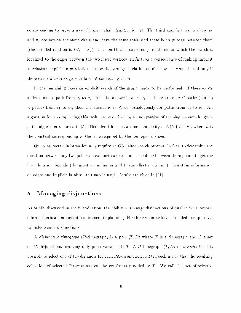
corresponding to p1; p2 are on the same chain (see Section 2). The third case is the one where v1and v2 are not on the same chain and have the same rank, and there is no 6= edge between them(the entailed relation is f<;=; >g). The fourth case concerns 6= relations for which the search islocalized to the edges between the two input vertices. In fact, as a consequence of making implicit< relations explicit, a 6= relation can be the strongest relation entailed by the graph if and only ifthere exists a cross-edge with label 6= connecting them.In the remaining cases an explicit search of the graph needs to be performed. If there existsat least one <-path from v1 to v2, then the answer is v1 < v2. If there are only �-paths (but no<-paths) from v1 to v2, then the answer is v1 � v2. Analogously for paths from v2 to v1. Analgorithm for accomplishing this task can be derived by an adaptation of the single-source-longest-paths algorithm reported in [5]. This algorithm has a time complexity of O(h + e + n), where h isthe constant corresponding to the time required by the four special cases.Querying metric information may require an O(e) time search process. In fact, to determine theduration between any two points an exhaustive search must be done between these points to get thebest duration bounds (the greatest minimum and the smallest maximum). Duration informationon edges and implicit in absolute times is used. Details are given in [21].5 Managing disjunctionsAs brie y discussed in the introduction, the ability to manage disjunctions of qualitative temporalinformation is an important requirement in planning. For this reason we have extended our approachto include such disjunctions.A disjunctive timegraph (D-timegraph) is a pair hT;Di where T is a timegraph and D a setof PA-disjunctions involving only point-variables in T . A D-timegraph hT;Di is consistent if it ispossible to select one of the disjuncts for each PA-disjunction in D in such a way that the resultingcollection of selected PA-relations can be consistently added to T . We call this set of selected10

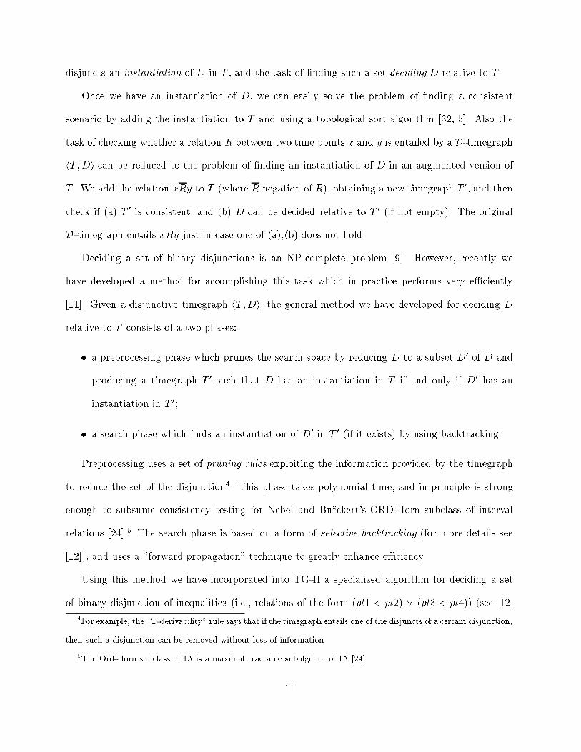
disjuncts an instantiation of D in T , and the task of �nding such a set deciding D relative to T .Once we have an instantiation of D, we can easily solve the problem of �nding a consistentscenario by adding the instantiation to T and using a topological sort algorithm [32, 5]. Also thetask of checking whether a relation R between two time points x and y is entailed by a D-timegraphhT;Di can be reduced to the problem of �nding an instantiation of D in an augmented version ofT . We add the relation xRy to T (where R negation of R), obtaining a new timegraph T 0, and thencheck if (a) T 0 is consistent, and (b) D can be decided relative to T 0 (if not empty). The originalD-timegraph entails xRy just in case one of (a),(b) does not hold.Deciding a set of binary disjunctions is an NP-complete problem [9]. However, recently wehave developed a method for accomplishing this task which in practice performs very e�ciently[11]. Given a disjunctive timegraph hT;Di, the general method we have developed for deciding Drelative to T consists of a two phases:� a preprocessing phase which prunes the search space by reducing D to a subset D0 of D andproducing a timegraph T 0 such that D has an instantiation in T if and only if D0 has aninstantiation in T 0;� a search phase which �nds an instantiation of D0 in T 0 (if it exists) by using backtracking.Preprocessing uses a set of pruning rules exploiting the information provided by the timegraphto reduce the set of the disjunction4. This phase takes polynomial time, and in principle is strongenough to subsume consistency testing for Nebel and Bu�rckert's ORD-Horn subclass of intervalrelations [24].5 The search phase is based on a form of selective backtracking (for more details see[12]), and uses a "forward propagation" technique to greatly enhance e�ciency.Using this method we have incorporated into TG-II a specialized algorithm for deciding a setof binary disjunction of inequalities (i.e., relations of the form (pt1 < pt2) _ (pt3 < pt4)) (see [12]4For example, the \T-derivability" rule says that if the timegraph entails one of the disjuncts of a certain disjunction,then such a disjunction can be removed without loss of information.5The Ord-Horn subclass of IA is a maximal tractable subalgebra of IA [24].11

for a detailed description of the algorithm). Such disjunctions extend the set of interval relationswhich are translatable in terms of point relations to include, in particular, \before or after" (intervaldisjointness), and exclusion of a point p1 form an interval with endpoints p2 and p3 (indicated belowas p1<#p2p3), where p2 < p3. In fact, we have:6I fB Ag J , (I:end < J:start) _ (J:end < I:start);p1<#p2p3 , ((p1 < p2) _ (p3 < p1)) ^ p2 < p3.Moreover, some 3-interval and 4-interval relations not belonging to IA can be also stipulated,for example: (I fBg J) or (H fBg K) , (I:end < J:start) _ (H:end < K:start).Experimental results have shown that our algorithm is very e�cient especially when the numberof disjunctions is limited with respect to the number of the PA-relations in the timegraph, and thatalthough consistency testing is NP-complete, in practice it performs polynomially (see Section 7).Future work concerns the extension of the algorithm in order include disjunctions of arbitraryPA-relations.6 TimeGraph I and IITimeGraph I (TG-I) and TimeGraph II (TG-II) are two temporal reasoning systems based on therepresentation and algorithms described in the previous Section. TG-I was originally developed inthe context of natural language comprehension and has been integrated into a series of knowledgerepresentation and reasoning systems, the two most recent being ECOLOGIC [27] and EPILOG[26, 15]. TG-II is an extension of TG-I which is still in progress and which aims at generalizing thetimegraph approach to a wider class of applications including planning and scheduling. Currentlythe most important extensions of TG-I which are incorporated into TG-II concern:6Ordering relations between starting point and end point of intervals are omitted.12

� the inclusion of algorithms for handling 6= relations which are not handled by TG-I and whichallow the representation of a larger class of interval relations;� the inclusion of algorithms for deciding a set of of binary disjunctions of inequalities relativeto the timegraph;� an optimization of the chain partitioning of the TL-graph built from an initial set S of pointrelations. In principle, many logically equivalent timegraphs may be constructed from S sincethere can be many di�erent ways to partition the TL-graph. TG-II attempts to minimize thenumber of chains and cross-edges;� new e�cient algorithms for computing the nextgreaters and for querying the timegraph, whichuse the rank to prune the search in the metagraph.The most important features of TG-I which have not been integrated into TG-II yet are the man-agement of metric information and the dynamic addition of new relations to the timegraph.Both TG-I and TG-II are written in Common Lisp. TG-II is available to the interested readervia FTP from cs.rochester.edu:/pub/knowledge-tools �les tg-ii*.76.1 The user interface of TG-I and TG-IIBoth TG-I and TG-II have a user interface which allows the assertion of relations between timepoints as well as between time intervals called episodes in TG-I.8The current TG-II's interface allows the assertion of all the relations in PA and of all the188 interval relations of SIA [18, 33] (see Figure 6) extended with relations expressing point-intervalexclusion and disjointness relations such as "before or after", which are representable through binarydisjunctions of inequalities (see Section 5).7The current version of TG-II available via FTP does not include the algorithms for managing disjunctions.8An Interval is represented as a pair of strictly ordered points corresponding to the starting and end time of theinterval. 13

fgfMgfBgfAgfEgfSgfFgfDgfOgfO-gfF-gfM-gfD-gfS-gfE SgfE S-gfS S-gfE S S-gfM BgfF- OgfF- D-gfO D-gfF- O D-gfM OgfM F- OgfM O D-gfM F- O D-gfB OgfB F- OgfB O D-gfB F- O D-gfM B OgfM B F- OgfM B O D-gfM B F- O D-gfE F-gfS OgfE S F- OgfS- D-gfE S- F- D-gfS S- O D-gfE S S- F- D- OgfS M OgfS M F- OgfS S- M O D-gfE S S- M F- O D-gfS B OgfE S B F- OgfS S- B O D-gfE S S- B F- O D-gfS M B OgfE S M B F- OgfS S- M B O D-gfE S S- M B F- O D-gfF DgfF O-gfD O-gfF D O-gfM- O-gfM- F O-gfM- D O-gfM- F D O-gfM- AgfO- AgfF O- AgfD O- AgfF D O- AgfM- O- AgfM- F O- AgfM- D O- AgfM- F D O- AgfE FgfS DgfE S F DgfS- O-gfE S- F O-g

fS S- D O-gfE S S- F D O-gfS- M- O-gfE S- M- F O-gfS S- M- D O-gfE S S- M- F D O-gfS- O- AgfE S- F O- AgfS S- D O- AgfE S S- F D O- AgfS- M- O- AgfE S- M- F O- AgfS S- M- D O- AgfE S S- M- F D O- AgfF- FgfO DgfF- O F DgfD- O-gfF- D- F O-gfO D- D O-gfF- O D- F D O-gfM O DgfM F- O F DgfM O D- D O-gfM F- O D- F D O-gfB O DgfB F- O F DgfB O D- D O-gfB F- O D- F D O-gfM B O DgfM B F- O F DgfM B O D- D O-gfM B F- O D- F D O-gfD- M- O-gfF- D- M- F O-gfO D- M- D O-gfF- O D- M- F D O-gfM O D- M- D O-gfM F- O D- M- F D O-gfB O D- M- D O-gfB F- O D- M- F D O-gfM B O D- M- D O-gfM B F- O D- M- F D O-gfD- O- AgfF- D- F O- AgfO D- D O- AgfF- O D- F D O- AgfM O D- D O- AgfM F- O D- F D O- AgfB O D- D O- AgfB F- O D- F D O- AgfM B O D- D O- AgfM B F- O D- F D O- AgfD- M- O- AgfF- D- M- F O- AgfO D- M- D O- AgfF- O D- M- F D O- AgfM O D- M- D O- AgfM F- O D- M- F D O- AgfB O D- M- D O- AgfB F- O D- M- F D O- AgfM B O D- M- D O- AgfM B F- O D- M- F D O- AgfE F- FgfS O DgfE S F- O F DgfS- D- O-gfE S- F- D- F O-gfS S- O D- D O-gfE S S- F- O D- F D O-gfS M O DgfE S M F- O F DgfS S- M O D- D O-gfE S S- M F- O D- F D O-gfS B O Dg

fE S B F- O F DgfS S- B O D- D O-gfE S S- B F- O D- F D O-gfS M B O DgfE S M B F- O F DgfS S- M B O D- D O-gfE S S- M B F- O D- F D O-gfS- D- M- O-gfE S- F- D- M- F O-gfS S- O D- M- D O-gfE S S- F- O D- M- F D O-gfS S- M O D- M- D O-gfE S S- M F- O D- M- F D O-gfS S- B O D- M- D O-gfE S S- B F- O D- M- F D O-gfS S- M B O D- M- D O-gfE S S- M B F- O D- M- F D O-gfS- D- O- AgfE S- F- D- F O- AgfS S- O D- D O- AgfE S S- F- O D- F D O- AgfS S- M O D- D O- AgfE S S- M F- O D- F D O- AgfS S- B O D- D O- AgfE S S- B F- O D- F D O- AgfS S- M B O D- D O- AgfE S S- M B F- O D- F D O- AgfS- D- M- O- AgfE S- F- D- M- F O- AgfS S- O D- M- D O- AgfE S S- F- O D- M- F D O- AgfS S- M O D- M- D O- AgfE S S- M F- O D- M- F D O- AgfS S- B O D- M- D O- AgfE S S- B F- O D- M- F D O- AgfS S- M B O D- M- D O- AgfE S S- M M- F F- O O- D D- A BgFigure 6: The interval relations of SIATG-I accepts assertions of relations in a subalgebra of PA called Convex Point Algebra (CPA)in [34] (i.e. the set of relations of PA with the exception of 6=), and of interval relations in a subclassof 83 relations of SIA (written as CSIA) which are listed in see [33]. It also accepts assertions aboutabsolute times and durations. On assertion, if an argument is an absolute time instead of a namedtime point or an interval, the appropriate absolute time of the other argument is updated. Forexample, (I before (date '1993 '04 '01 '00 '00 '00)) would update the upper bound of I 's absolutetime (the maximum). For evaluation, the appropriate bound is compared against the absolute time,or two absolute times may be compared.In addition, some predicates have been introduced to handle durations: at-most-before,at-most-after,at-least-before,at-least-after, exactly-before, and exactly-after. These take three arguments, ofwhich the �rst two may be intervals or time points (no absolute times) and the third denotesthe duration between the two in seconds. At-most- implies maximum duration, at-least- impliesminimum duration, and exactly- involves both (see Tables 2, 3 and 4).14

Argument1 Relation Argument2 Argument3Sort Sort Sortepisode equal episodepoint same-time pointepisode CSIA-relation episodepoint CPA-relation pointepisode between episode episodepoint point pointepisode at-most-before episode numberpoint at-least-before pointexactly-beforeexactly-afterat-most-afterat-least-afterepisode has-duration numberTable 2: The relations accepted by TG-I. In all patterns except the second last group (with at-most...), a point argument may be either a named time point or an absolute time speci�cation. Forthe second last group, a point argument must be a named time pointListed below are some of the main of user-interface functions9 recognized by TG-I and TG-II(the strongest entailed relation between two points pt1 and pt2 (intervals I1 and I2) is indicatedwith SER(pt1,pt2) (SER(I1,I2)); optional arguments are enclosed by h i.� (make-event arg) [TG-I]This functions creates an interval named arg and asserts arg:start < arg:end, where arg:startis the starting point of arg and arg:end is the end point. Make-event is de�ned only in TG-I,since in TG-II time points and intervals are automatically created when relations are asserted.� (asserta arg1 reln arg2) [TG-I/II]This function is present both in TG-I and TG-II. It asserts that the relation between arg1 andarg2 is reln. For a description of the relations accepted by TG-I see Table 2. In TG-II arg1 andarg2 must be intervals,10 and reln one of the interval relations of SIA (see Figure 6) extended9The actual implementation of most of them is in form of a Lisp \macro".10Point relations can be expressed using the function \assertpr".15

Relation Meaning (e1 relation e2 e3)between-0-0 e1:end = e2:start and e2:end = e3:startbetween-1-0 e1:end < e2:start and e2:end = e3:startbetween--0 e1:end � e2:start and e2:end = e3:startbetween-0-1 e1:end = e2:start and e2:end < e3:startbetween-0 e1:end = e2:start and e2:end � e3:startbetween-1-1 e1:end < e2:start and e2:end < e3:startbetween-1 e1:end < e2:start and e2:end � e3:startbetween--1 e1:end � e2:start and e2:end < e3:startbetween e1:end � e2:start and e2:end � e3:startTable 3: The between-relations of TG-I. e:start and e:end indicate respectively the starting pointand the end point of the interval (episode) e; "1" indicates strict (<); "0" indicates equal (meets),and nothing indicates non-strict (�)Relation Meaning (e1 relation fe2g d)at-most-before e1 fB Mg e2 and maximum duration between them is dat-least-before e1 fBg e2 and minimum duration between them is dexactly-before e1 fBg e2 and both maximum and minimum durations are dat-most-after e1 fA M-g e2 and maximum duration between them is dat-least-after e1 fAg e2 and minimum duration between them is dexactly-after e1 fAg e2 and both maximum and minimum durations are dhas-duration e1.start before e1.end and duration of e1 is dTable 4: The metric relations of TG-Iby interval relations which can be expressed in terms of binary disjunctions of inequalities (seeSection 5.)� (assertpr pt1 reln pt2) [TG-II]This function asserts that the relation between pt1 and pt2 is reln, where reln is one of:=; <;>;�;�; 6=.� (make-tg ) [TG-II]This function builds the timegraph from the set of the stipulated relations. Note that in TG-Ithe timegraph is always built incrementally.11.� (decide-disjunctions D) [TG-II]11In TG-I the timegraph is automatically updated after each assertion.16

This function decides of a set D of disjunctions relative to the timegraph. In the currentimplementation D can be a set of binary disjunctions of inequalities only.� (reln arg1 arg2) [TG-I]This function returns SER(arg1,arg2), where arg1 and arg2 may be episodes, time points, orabsolute times.� (elapsed pt1 pt2) [TG-I]This function returns the best duration bounds between two time points (pt1 and pt2) as aquoted expression of the form (minimum maximum).� (duration-of e1) [TG-I]This function returns the duration bounds between the start of an episode and its end as aquoted expression of the form (minimum maximum).� (prel hpt1 hpt2ii) [TG-II]When both the arguments are present this function returns the SER(pt1,pt2); when only pt1is given it returns SER(pt1,x) for all the time points x of the timegraph; when none of thearguments is present it returns SER(x,y) for all the time points x and y of the timegraph. Ifthe timegraph has not been built yet, the set of the stipulated relations is printed.� (arel hI1 hI2ii) [TG-II]When both the arguments are present this function returns the SER(I1,I2); when only I1 isgiven it returns SER(X1,x) for all the time intervals x in the timegraph; when none of thearguments is given it returns the SER(x,y) for all the time intervals x and y in the timegraph.If the timegraph has not been built yet, the set of the stipulated is printed.� (less-than pt1 pt2) [TG-II]This function returns T when SER(pt1,pt2) is <; it returns NIL when SER(pt1,pt2) is �; itreturns unknown in the other cases. 17

� (less-or-equal pt1 pt2) [TG-II]This function returns T when SER(pt1,pt2) is �; it return NIL when SER(pt1,pt2) is >; itreturns unknown in the other cases.� (greater-than pt1 pt2) [TG-II]This function returns T when SER(pt1,pt2) is >; it return NIL when SER(pt1,pt2) is �; itreturns unknown in the other cases.� (greater-or-equal pt1 pt2) [TG-II]This function returns T when SER(pt1,pt2) is �; it returns NIL when SER(pt1,pt2) is <; itreturns unknown in the other cases.� (equal-to pt1 pt2) [TG-II]This function returns T when SER(pt1,pt2) is =; it returns NIL when SER(pt1,pt2) is <,> or6=; it returns unknown in the other cases.� (not-equal-to pt1 pt2) [TG-II]This function returns T when SER(pt1,pt2) is <,> or 6=; it returns NIL when SER(pt1,pt2)is =; it returns unknown in the other cases.� (pointizable reln)This functions returns T if reln is a pointizable interval relation, i.e. it is an interval relationsof SIA.� (print-tg ) [TG-II]This function prints the following information about the timegraph and the metagraph: thelength, the starting point and the end point of each chain; the nextgreater and the prevlesslinks of each vertex; all the metavertices (cross-connected vertices) with the relative metaedges(cross-edges). 18

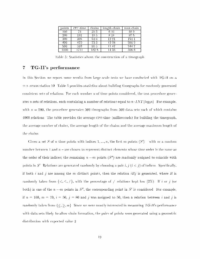
points cpu-time chains length-chain max-chain100 74 20.3 6.10 48.9200 191 40.5 8.18 97.5300 308 54.6 12.21 154.1400 470 73.3 12.28 206.2500 592 96.5 11.47 244.71000 1711 182.8 14.36 508.8Table 5: Statistics about the construction of a timegraph7 TG-II's performanceIn this Section we report some results from large scale tests we have conducted with TG-II on asun sparcstation 10. Table 5 provides statistics about building timegraphs for randomly generatedconsistent sets of relations. For each number n of time points considered, the test procedure gener-ates n sets of relations, each containing a number of relations equal to n �INT (log2n). For example,with n = 500, the procedure generates 500 timegraphs from 500 data sets each of which contains4000 relations. The table provides the average cpu-time (milliseconds) for building the timegraph,the average number of chains, the average length of the chains and the average maximum length ofthe chains.Given a set S of n time points with indices 1; :::; n, the �rst m points (S 0) { with m a randomnumber between 1 and n { are chosen to represent distinct elements whose time order is the same asthe order of their indices; the remaining n�m points (S 00) are randomly assigned to coincide withpoints in S 0. Relations are generated randomly by choosing a pair i; j (i < j) of indices. Speci�cally,if both i and j are among the m distinct points, then the relation iRj is generated, where R israndomly taken from f<;�; 6=g, with the percentage of 6= relations kept low (2%). If i or j (orboth) is one of the n �m points in S 00, the corresponding point in S 0 is considered. For example,if n = 100, m = 70, i = 50, j = 80 and j was assigned to 50, then a relation between i and j israndomly taken from f�;�;=g. Since we were mostly interested in measuring TG-II's performancewith data sets likely to allow chain formation, the pairs of points were generated using a geometricdistribution with expected value 3. 19

Other experiments show that querying a timegraph is on average a fast operation. For example,the average cpu-time over 100,000 queries on 100 randomly generated timegraphs with 500 pointswas 2.8 milliseconds.The curves in Figure 7 report the results of an experiment aimed at testing the scalabilityof TG-II for the task of deciding randomly generated consistent set of disjunctions (see [12] formore details). The two curves of the �rst graph show the average cpu-time (seconds) required fordeciding sets of disjunctions of size n (for n the number of time points) with 8n and 2nlogn simplePA-relations (with the logarithm truncated to its integer part). The numbers attached to the pointson the curve indicate the percentage of the disjunctions eliminated by preprocessing. While in thecase of 8n relations this percentage decreases when n increases, for 2nlogn relations it tends to beconstant (wavering between 88.8 and 91.3).12The curve in the second graph shows the average cpu-time required by more sparse graphs (4nPA-relations) for which forward propagation has been used during the search.13The third graph shows that for the 16,000 problems considered our algorithms tend to performpolynomially (quadratic time for the curves of the �rst graph and cubic time for the curve of thesecond) since the previous curves approximate straight lines on a log{log scale.Finally, we should mention some experiments conducted by Yampratoom and Allen [36] com-paring the performance of Timegraph I and II with several temporal reasoning systems based onconstraint propagation algorithms { TimeLogic [17], MATS [16], Tachyon [4] and TMM [6] { inwhich the timegraph approach proved by far the most e�cient for large data sets generated for theTRAINS world [1].12In order to simplify the �gure these numbers are not shown.13These experiments were conducted on a sun sparcstation 2 and hence a comparison with the results in theprevious graph is inappropriate. 20

1234550 100 150 200 250 300 350 400CPU-time no prop. (8000 problems)88.983.5 80 77.8 76.174.373.271.9sec. points and disjunctions8n rels. 33 3 3 3 3 3 3 32nlogn-rels. ++ + + + + + + + 5015025035045050 100 150 200 250 300 350 400CPU-time with prop. (8000 problems)points and disjunctionssec. 66.255.448.844.2 4139.136.735.14n rels. 22 2 2 2 2 2 2 2 0.010.1110100100050 100 200 300 400CPU-time (log. scale)points and disjunctionssec.3 3 3 3 3 333+ + + + + +++2 2 2 2 2 2 22Figure 7: Scalability of the algorithms for deciding a set of disjunctions8 Conclusions and future workWe have described two e�cient domain-independent temporal reasoning systems. Our approach isrelated to others recently proposed [8, 13] and whose main characteristic is that of providing betterperformance in practice compared to the more traditional constraint-based approaches.In particular, in our systems both space and time complexity are reduced signi�cantly for manypractical applications. In fact, the space complexity depends on the size of the set of the stipulatedrelations and on a limited number of implicit <-relations (those araising from 6= diamonds), and noton the number of time points (as in the constraint propagation approach). Instead of computingthe closure of the set of relations in PA or SIA, we build timegraph providing a collection of datastructures that allow e�cient deduction of relations at query time.TG-I can handle the qualitative relations of CPA and CSIA, and metric information such asdurations and absolute times. TG-II considerably extends the expressiveness of TG-I at the qual-itative level by including e�cient algorithms for managing 6=-relations and binary disjunctions ofinequalities, allowing the representation of all the interval relations of SIA, as well as point-intervalexclusion and interval disjointness. Experimental results have shown that TG-II is much faster thatother systems based on constraint propagation.Current and future work on TG-II concerns the design of e�cient algorithms for adding new21

relations to the timegraph dynamically, the integration of metric relations,14 and the design andimplementation of an e�cient algorithm for handling disjunctions of arbitrary PA-relations.References[1] J. Allen and L. Schubert. The trains project. Technical Report 91-1, Department of ComputerScience, University of Rochester, Rochester, NY, 1991.[2] J. F. Allen, H. Kautz, R. Pelavin, and J. Tenenberg. Reasoning about Plans. Morgan-Kaufmann,San Mateo, CA, 1991.[3] J. F. Allen and J. A. Koomen. Planning using a temporal world model. In Proceedings ofthe Eighth International Joint Conference on Arti�cial Intelligence, pages 741{747, Karlsruhe,Germany, 1983.[4] R. Arthur and J. Stillman. Temporal reasoning for planning and scheduling. user's guide: Pre-liminary realise. Technical report, Arti�cial Intelligence Laboratory, General Electric Researchand Development Center, 1992.[5] T. Cormen, C. Leiserson, and R. Rivest. Introduction to Algorithms. The MIT Press, 1990.[6] T. Dean and D. V. McDermott. Temporal data base management. Arti�cial Intelligence,32:1{55, 1987.[7] R. Dechter, I. Meiri, and J. Pearl. Temporal constraint networks. Arti�cial Intelligence, 49:61{95, 1991.[8] J. Dorn. Temporal reasoning in sequence graphs. In Proceedings of the Tenth National Confer-ence of the American Association for Arti�cial Intelligence (AAAI-92), pages 735,740, 1992.14These were handled in TG-I, but as noted 6= was not handled and also < and � relations entailed via metricrelations were not extracted in a deductively complete way.22

[9] A. Gerevini and L. Schubert. Complexity of temporal reasoning with disjunctions of in-equalities. In Workshop notes of the IJCAI-93 Workshop on spatial and temporal reasoning,Chamb�ery, Savoie, France, 1993. Also available as: Technical Report 9303-01, IRST - Istitutoper la Ricerca Scienti�ca e Tecnologica, 38050 Povo, Trento Italy.[10] A. Gerevini and L. Schubert. E�cient temporal reasoning through timegraphs. In Proceedingsof the Thirteenth International Joint Conference on Arti�cial Intelligence (IJCAI-93), pages648{654, Chamb�ery, Savoie, France, 1993.[11] A. Gerevini and L. Schubert. An e�cient method for managing disjunctions in qualitativetemporal reasoning. In Principles of Knowledge Representation and Reasoning: Proceedingsof the Fourth International Conference (KR94), San Francisco, CA, 1994. Morgan Kaufmann.Forthcoming.[12] A. Gerevini and L. Schubert. E�cient algorithms for qualitative reasoning about time. Arti�cialIntelligence, to appear. Also available as: IRST Technical Report 9307-44, Istituto per laRicerca Scienti�ca e Tecnologica, 38050 Povo, Trento Italy.[13] M. Ghallab and A. Mounir Alaoui. Managing e�ciently temporal relations through indexedspanning trees. In Proceedings of the Eleventh International Joint Conference on Arti�cialIntelligence (IJCAI-89), pages 1297{1303, 1989.[14] M. Golumbic and R. Shamir. Algorithms and complexity for reasoning about time. In Proceed-ings of the Tenth National Conference of the American Association for Arti�cial Intelligence(AAAI-92), pages 741{746, 1992.[15] C. H. Hwang and L. H. Schubert. Meeting the interlocking needs of lf-computation, deindexing,and inference: An organic approach to general nlu. In Proceedings of the Thirteenth Interna-tional Joint Conference on Arti�cial Intelligence (IJCAI-93), Chamb�ery, Savoie, France, 1993.23

[16] H. Kautz and P. Ladkin. Integrating metric and qualitative temporal reasoning. In Proceed-ings of the Nineth National Conference of the American Association for Arti�cial Intelligence,Anheim, Los Angeles, CA, 1991.[17] Johannes A. G. M. Koomen. The timelogic temporal reasoning system. Technical Report 231,University of Rochester, Computer Science Dept. Rochester New York 14627, 1988.[18] P. Ladkin and R. Maddux. On binary constraint networks. Technical Report KES.U.88.8,Kestrel Institute, Palo Alto, CA, 1988.[19] P. Ladkin and R. Maddux. On binary constraint problems. Journal of the Association forComputing Machinery (ACM), to appear.[20] P. Ladkin and A. Reinefeld. E�ective solution of qualitative interval constraint problems.Arti�cial Intelligence, 57(1):105{124, 1992.[21] S. A. Miller. Time revised. Technical Report M.Sc. thesis, Dept. of Computer Science, TheUniversity of Alberta, Edmonton, Alta, 1988.[22] S. A. Miller and L. K. Schubert. Time revisited. Computational Intelligence, 6:108{118, 1990.[23] U. Montanari. Networks of constraints: Fundamental properties and applications to pictureprocessing. Information Science, 7(3):95{132, 1974.[24] B. Nebel and H. J. B�urckert. Reasoning about temporal relations: A maximal tractable subclassof Allen's interval algebra. Research Report RR-93-11, German Research Center for Arti�cialIntelligence (DFKI), Saarbr�ucken, Germany, March 1993.[25] J.S. Penberthy and D. Weld. Ucpop: A sound, complete, partial order planner for adl. InProceedings of the Third International Conference on Principles of Knowledge Representationand Reasoning, pages 103{114, 1992.[26] S. A. Schae�er, C. H. Hwang, J. de Haan, and L. K. Schubert. The user's guide to epilog.Technical report, Dept. of Computing Science, Univ. of Alberta, Edmonton, Alberta, Canada,1991. 24

[27] L. K. Schubert and C. H. Hwang. An episodic knowledge representation for narrative texts. InProceedings of the First International Conference on Principles of Knowledge Representationand Reasoning, pages 444{458, Toronto, Ont., 1989.[28] L. K. Schubert, M. A. Papalaskaris, and J. Taugher. Determining type, part, colour, and timerelationships. Computer (special issue on Knowledge Representation), 16:53{60, 1983.[29] L. K. Schubert, M. A. Papalaskaris, and J. Taugher. Accelerating deductive inference: Specialmethods for taxonomies, colours, and times. In N. Cercone and G. McCalla, editors, TheKnowledge Frontier: Essays in the Representation of Knowledge, pages 187{220. Springer-Verlag, Berlin, Heidelberg, New York, 1987.[30] J. Taugher. An e�cient representation for time information. In M.Sc. thesis, Department ofComputer Science, University of Alberta, Edmont, Alta, 1983.[31] P. van Beek. Reasoning about qualitative temporal information. In Proceedings of the EighthNational Conference of the American Association for Arti�cial Intelligence (AAAI-90), pages728{734, Boston, MA, 1990.[32] P. van Beek. Reasoning about qualitative temporal information. Arti�cial Intelligence, 58(1-3):297{321, 1992.[33] P. van Beek and R. Cohen. Exact and approximate reasoning about temporal relations. Com-putational Intelligence, 6:132{144, 1990.[34] M. Vilain and H. Kautz. Constraint propagation algorithms for temporal reasoning. In Pro-ceedings of the Fifth National Conference of the American Association for Arti�cial Intelligence(AAAI-86), pages 377{382, Philadelphia, PA, 1986.[35] D. S. Weld. An introduction to least commitment planning. AI Magazine, Fall 1994, to appear.[36] E. Yampratoom and J. Allen. Performance of temporal reasoning systems. SIGART Bulletin,4(3), 1993. 25