Reasoning with Uncertainty in Continuous Domains

Reasoning with Uncertainty in ContinuousDomains

Elsa Carvalho, Jorge Cruz, and Pedro Barahona

Abstract Continuous constraint programming has been widely used to model safereasoning in applications where uncertainty arises. Constraint propagation propa-gates intervals of uncertainty among the variables of the problem, eliminating val-ues that do not belong to any solution. However, to play safe, these intervals maybe very wide and lead to poor propagation. We proposed a probabilistic continu-ous constraint framework that associates a probabilistic space to the variables of theproblem, allowing to distinguish between different scenarios, based on their likeli-hoods. In this paper we discuss the capabilities of the framework for decision sup-port in nonlinear continuous problems with uncertain information. Its applicabilityis illustrated in inverse and reliability problems, which are two different types ofproblems representative of the kind of reasoning required by the decision makers.

1 Introduction

A mathematical model describes a system by a set of variables and a set of con-straints that establish relations between the variables. Uncertainty and nonlinearityplay a major role in modeling real-world continuous systems. When the model ishighly nonlinear small approximation errors may be highly magnified. Any frame-work for decision support in continuous domains must provide an expressive math-ematical model to represent the system behavior and be able to perform sound rea-soning that accounts for the uncertainty and the effect of nonlinearity. Given theuncertainty, there are two classical approaches to reason with the possible scenariosconsistent with the mathematical model.

When safety is a major concern all possible scenarios must be predicted. Forthat purpose, rather than associate approximate values to variables, intervals can beused to include all their possible values. This is the approach adopted in continuous

Centro de Inteligencia Artificial, Universidade Nova de Lisboa, [email protected], {jc,pb}@di.fct.unl.pt

1

2 E. Carvalho, J. Cruz, P. Barahona

constraint programming [18, 1] which uses safe constraint propagation techniques tonarrow the intervals thus reducing uncertainty. Nevertheless this approach considersall the scenarios to be equally likely, leading to great inefficiency if some costlydecisions are taken due to very unlikely scenarios.

In contrast, stochastic approaches reason on approximations of the most likelyscenarios. They associate a probabilistic model to the problem characterizing thelikelihood of the different scenarios. Some methods use local search approximationtechniques to finding the most likely scenario, which may lead to erroneous deci-sions due to approximation errors and nonlinearity. Moreover, there may be othersatisfactory scenarios to decision making which are ignored by this single scenarioapproach. Other stochastic methods use aim extensive random sampling over thedifferent scenarios to characterize the complete probability space. However, evenafter intensive computations, no definite conclusion can be drawn with these meth-ods, because a significant subset of the probabilistic space may have been missed.

We proposed an extension to the classical continuous constraint approach to com-plement the interval bounded representation of uncertainty with a probabilistic char-acterization of the values distributions [3]. In this paper we argue that this constitutesan attractive approach to decision support in the presence of uncertainty, bridgingthe gap between pure safe reasoning and pure probabilistic reasoning.

There are a number of works that combine probabilities and constraint program-ming [21, 8, 23] or represent the uncertainty associated with the modeled problems[2] but they deal with discrete domains and, consequently, both the techniques andthe modeled problems are necessarily different.

Our approach is applied to inverse and reliability problems. Inverse problems aimto estimate parameters from observed data based on a model of the system behavior.Uncertainty arises from measurement errors on the observed data or approximationsin the model specification. Reliability problems aim to find reliable decisions ac-cording to a model of the system behavior, where both decision and uncontrollablevariables may be subject to uncertainty. Given the choices committed in a decision,its reliability quantifies the ability of the system to perform the required functions.

2 Continuous Constraint Programming

A Continuous Constraint Satisfaction Problem (CCSP) is defined by a set of realvalued variables and a set of constraints on subsets of the variables. A solution is avalue assignment to all variables satisfying all the constraints.

Constraint reasoning aims at eliminating value combinations from the initial do-mains (the initial search space) that do not satisfy the constraints. Usually, duringconstraint reasoning in continuous domains, the search space is maintained as a setof boxes (Cartesian product of intervals) which are pruned and subdivided until astopping criterion is satisfied (e.g. all boxes are small enough).

The pruning of the variable domains is based on constraint propagation. For thispurpose, narrowing functions (mappings between boxes) are associated with con-straints, often implementing efficient methods from interval analysis (e.g. the inter-

Reasoning with Uncertainty in Continuous Domains 3

val Newton [20]) to guarantee correctness (elimination of no solutions) and con-tractness (the box obtained is smaller or equal than the original one).

In classical CCSPs, the uncertainty associated with the problem is modeled byusing intervals to represent the domains of the variables. Constraint reasoning re-duces uncertainty providing a safe method for computing a set of boxes enclosingthe feasible space. To play safe, the initial interval domains may be very wide, lead-ing to poor propagation and consequently to a wide enclosure of the regions thatmight contain the most likely solutions. This paradigm cannot distinguish betweendifferent scenarios and thus all combination of values within such enclosure areconsidered equally plausible.

3 Probabilistic Continuous Constraints

Probability provides a classical model for dealing with uncertainty [12]. The ba-sic element of probability theory is the random variable with an associated domainwhere it can assume values. In particular, continuous random variables assume realvalues. A possible world, or atomic event, is an assignment of values to all the vari-ables of the model. An event is a set of possible worlds. The complete set of allpossible worlds in the model is the sample space. If all random variables are con-tinuous, the sample space is the Cartesian product of the variable domains, and thepossible worlds and events are, respectively, points and regions on such hyperspace.

Probability measures may be associated with events. A probabilistic model is anencoding of probabilistic information, allowing to compute the probability of anyevent, in accordance with the axioms of probability. In the continuous case, the usualmethod for specifying a probabilistic model assumes, either explicitly or implicitly,a full joint probability density function (p.d.f.), which assigns a probability measureto each point of the sample space. Such assignment is representative of the likeli-hood in its neighborhood. The probability of any event E, given a p.d.f. f , is itsmulti-dimensional integral on the region defined by the event:

P(E) =∫

Ef (x)dx (1)

In accordance with the axioms of probability, f must be a non-negative functionand, when the event E is the complete sample space, the above integral must be 1.

To complement the interval bounded representation of uncertainty with a proba-bilistic characterization of the value distributions, the authors proposed the Proba-bilistic CCSP (PCCSP) [3] as an extension of a CCSP.

In a PCCSP (X ,D,C, f ), X is a tuple of n real variables 〈x1, . . . ,xn〉, D is theCartesian product of their domains I1×·· ·× In, with each variable xi ranging overthe real interval Ii, C is a finite set of numerical constraints on subsets of the variablesin X , and f is a non-negative point function defined in D such that:∫

I1. . .

∫

Inf (x1, . . . ,xn)dxn . . .dx1 = 1 (2)


The framework extends a CCSP associating a probabilistic model to its initialsearch space D characterized by a full joint p.d.f. f and the probability of any eventE may be theoretically computed as in (1). In particular, the feasible space F is theevent containing all possible points that satisfy the constraints.

In general such multi-dimensional integral cannot be easily computed since theevent E may establish a nonlinear integration boundary for which there is no closed-form solution. To compute a multi-dimensional integral of a nonlinear integrationarea, this area is safely approximated through discretization into a set of boxes en-closing it E ⊆ {B1, . . . ,Bk}. Then, the integrals of all boxes P(Bi) are computed andsummed up to obtain an approximation of the original integral. A safe lower boundfor the probability value, corresponds to sum the contributions of all boxes com-pletely included in the original area whereas a safe upper bound corresponds to sumthe contributions of all boxes that are included or intersect with the original area:

∑Bi⊆E

P(Bi)≤ P(E)≤ ∑Bi∩E 6= /0

P(Bi) (3)

The PCCSP framework provides a safe method to compute the probability P(F)of the feasible space. A set of boxes enclosing F is firstly obtained through con-straint reasoning. For this purpose we use an hypergrid over the entire search space,forcing each of the final enclosing boxes either to be completely included in the fea-sible space or to be an hypergrid-box that intersects with it. Such enclosure is thenused, according to (3), to compute safe bounds for the multi-dimensional integralwhich are closer to the correct value when the hypergrid granularity gets smaller.

Moreover, for any box B the probability P(F ∩B) is similarly computed if eachbox enclosing the feasible space is previously intersected with B. Furthermore, theprobability of B given the feasible space F is calculated by the conditional proba-bility rule P(B|F) = P(B∩F)/P(F). See [3] for implementation details.

The ability of the PCCSP framework for combining feasibility, through con-straint reasoning, and probability providing a safe method to reason with a prob-abilistic model, makes it potentially appealing for decision support in nonlinearcontinuous problems with uncertain information.

4 Inverse Problems

Inverse problems aim to estimate parameters from observed data based on a modelof the system behavior. The variables are the model parameters whose values com-pletely characterize the system, and the observable parameters which are measured.Usually a forward model defines a mapping from the model parameters to the ob-servable parameters allowing to predict measurements from the model parameters.

The forward mapping is commonly represented as a vector function G from theparameter space m (model parameters) to the data space d (observable parameters):

d = G(m) (4)


Such relation may be represented explicitly by an analytical formula or implicitlyby a complex system of equations or some special purpose algorithm.

Nonlinearity and uncertainty play a major role in modeling the behavior of mostsystems. An inverse problem may have no exact solutions, since usually there are nomodel parameter values capable of predicting exactly all the observed data. There-fore uncertainty, mainly due to model approximations and measurement errors, mustbe included in the model. When the model is highly nonlinear, uncertainty may bedramatically magnified, and an arbitrarily small change in the data may induce anarbitrarily large change in the values of the model parameters.

4.1 Alternative Approaches to Inverse Problems

Nonlinear inverse problems are classically handled as curve fitting problems [19].Such approaches are based on nonlinear regression methods which search for themodel parameter values that best-fit a given criterion. For instance, the least squarescriterion minimizes a quadratic norm of the difference between the vectors of ob-served data and model predictions. The minimization criteria are justified by thehypothesis that all uncertainties may be modeled using a well behaved distribution.

In nonlinear inverse problems where no explicit formula can be provided forobtaining the best-fit values, minimization is often performed through local searchalgorithms. However, the search method may stop at a local minimum with no guar-antees on the complete search space. Moreover a single best-fit solution may notbe enough since other solutions could also be satisfactory and so, the uncertaintyaround them should be characterized. The use of analytic techniques for this pur-pose must rely on some special assumptions about the model parameter distributions(for instance, assuming a single maximum). However, if the problem is highly non-linear, such assumptions do not provide realistic approximations for the uncertainty.

Other stochastic approaches [22] associate a probabilistic model to the problem,allowing to obtain any statistical information on the parameters. These approachestypically rely on extensive random sampling (Monte Carlo) to characterize the pa-rameter space. Nevertheless, only a number of discrete points of the continuousmodel space is analyzed and the results must be extrapolated to characterize theoverall uncertainty. To provide better uncertainty characterizations the samplingneeds to be reinforced in highly nonlinear problems. Contrary to constraint reason-ing approaches, these probabilistic techniques cannot prune the search space basedon model information, and so the entire space must be considered for exploration.

In contrast, bounded-error approaches [16, 10] characterize the set of all solutionsconsistent with the uncertainty on the parameters, the forward model and the data.Bounded-error estimation assumes initial intervals to each problem variable andsolves a CCSP with the set of constraints representing the forward model. It assumesprior knowledge on the acceptable parameter ranges and on the uncertainty about thedifference between predicted and observed data. From the safe approximation of thefeasible space, a projection on the set of model parameters (or a subset of it) providesinsight on the remaining uncertainty about their possible value combinations.


The formulation of an inverse problem as a CCSP allows its application when aforward model is not defined by an explicit analytical formula but by a complex setof relations. Furthermore, it may easily accommodate additional requirements, inthe form of constraints, which are more difficult to enforce in classical approaches.However, in most inverse problems, there is also additional knowledge about theplausibility distributions of values within the bounds of some uncertain parameters,which are not representable in the CCSP model. For instance, uncertainty due tomeasuring errors may be naturally associated with an error distribution.

4.2 Probabilistic Continuous Constraints for Inverse Problems

The application of the PCCSP framework to inverse problems [4], similarly tobounded-error estimation, assumes prior knowledge on the acceptable parameterranges and on the uncertainty about the difference between predicted and observeddata. However, the use of intervals to bound initial uncertainty is complemented withan explicit joint p.d.f. to represent prior information about the values distributions.

Any nonlinear inverse problem as specified in (4) may be represented by aPCCSP (X ,D,C, f ) where X are the model and observable parameters, D is theCartesian product of their initial ranges, C is a set of constraints representing theforward model, and f is the joint p.d.f. representing the available prior probabilityinformation. When the random variables are independent (which is usually the casefor the observed parameters whose error distributions may be considered indepen-dent) the joint p.d.f. is the product of their individual densities. If prior informationis unavailable, uniform distributions may be considered.

Once established a PCCSP for representing an inverse problem, the probabilityof any combination of parameter values given the observed data can be computed asthe conditional probability of such combination given the feasible space F . There-fore, complementary to the safe approximation of the feasible space, the frameworkprovides insight on the a posteriori distribution of the resulting narrowed ranges.

Consider the example of a nonlinear inverse problem extracted from [22]. Thegoal is to estimate the epicentral coordinates of a seismic event. The seismic wavesproduced have been recorded at a network of six seismic stations at different arrivaltimes. Table 1 presents their coordinates and the observed arrival times.

Table 1 Arrival times of the seismic waves observed at six seismic stations.(xi,yi) (3 km,15 km) (3 km,16 km) (4 km,15 km) (4 km,16 km) (5 km,15 km) (5 km,16 km)

ti 3.12 s 3.26 s 2.98 s 3.12 s 2.84 s 2.98 s

It is assumed that: seismic waves travel at a constant velocity of v = 5km/s;experimental uncertainties on the arrival times are independent and can be modeledusing a Gaussian probability density with a standard deviation σ = 0.1s.

Clearly, the model parameters are the epicentral coordinates (m0,m1) of the seis-mic event, and the observable parameters are the six arrival times di which are re-


lated by a forward model with six equations (one for each seismic station i):

di = Gi(m0,m1) =1v

√(xi−m0)

2 +(yi−m1)2 (5)

To represent this inverse problem by a PCCSP we define acceptable initial rangesfor the parameters of the problem, which are unbounded for the two model param-eters and [ti−3σ , ti +3σ ] for the six observable parameters. The constraints are thesix equations of the forward model (5). The joint p.d.f. is the product of the pa-rameter densities, which are Gaussians N(ti,σ) for the observable parameters andUniform densities for the model parameters (no prior information is available).

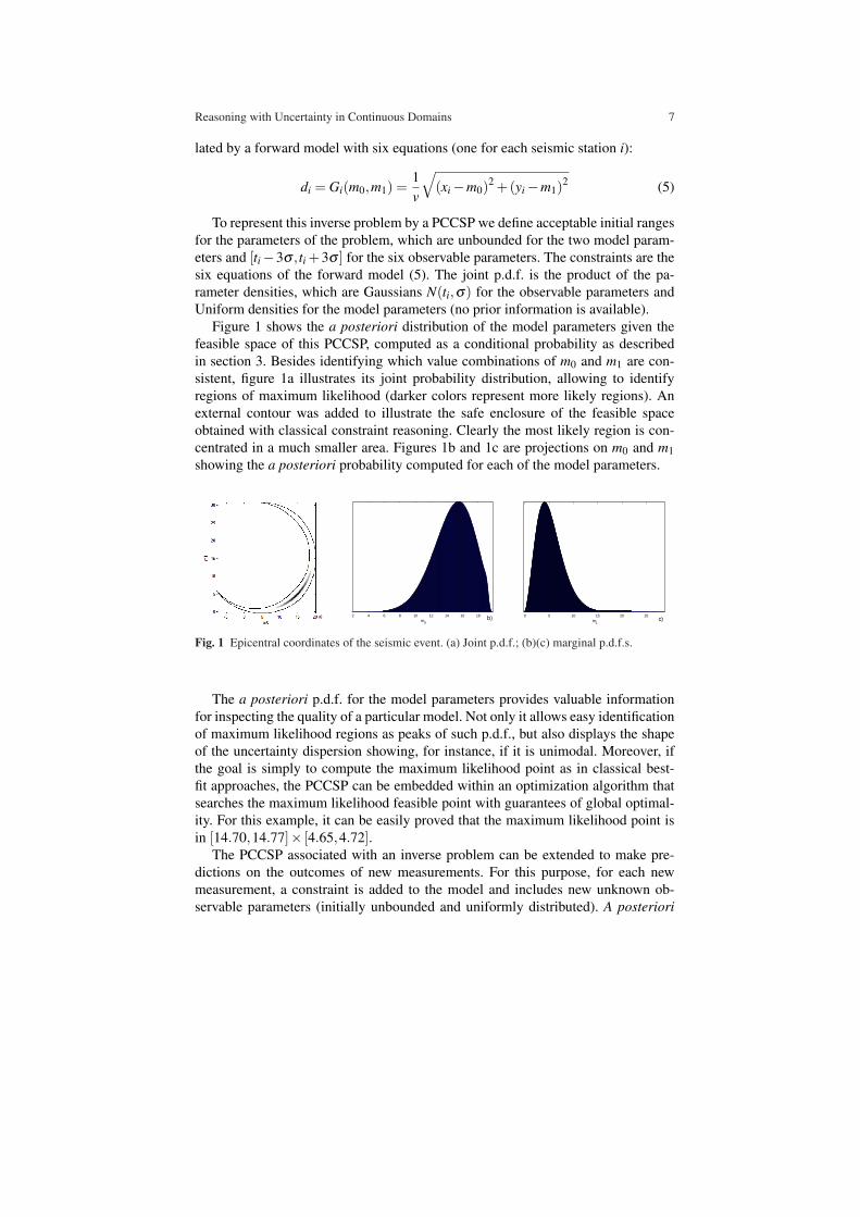
Figure 1 shows the a posteriori distribution of the model parameters given thefeasible space of this PCCSP, computed as a conditional probability as describedin section 3. Besides identifying which value combinations of m0 and m1 are con-sistent, figure 1a illustrates its joint probability distribution, allowing to identifyregions of maximum likelihood (darker colors represent more likely regions). Anexternal contour was added to illustrate the safe enclosure of the feasible spaceobtained with classical constraint reasoning. Clearly the most likely region is con-centrated in a much smaller area. Figures 1b and 1c are projections on m0 and m1showing the a posteriori probability computed for each of the model parameters.

a) 2 4 6 8 10 12 14 16 18m0

b)0 5 10 15 20 25

m1c)

Fig. 1 Epicentral coordinates of the seismic event. (a) Joint p.d.f.; (b)(c) marginal p.d.f.s.

The a posteriori p.d.f. for the model parameters provides valuable informationfor inspecting the quality of a particular model. Not only it allows easy identificationof maximum likelihood regions as peaks of such p.d.f., but also displays the shapeof the uncertainty dispersion showing, for instance, if it is unimodal. Moreover, ifthe goal is simply to compute the maximum likelihood point as in classical best-fit approaches, the PCCSP can be embedded within an optimization algorithm thatsearches the maximum likelihood feasible point with guarantees of global optimal-ity. For this example, it can be easily proved that the maximum likelihood point isin [14.70,14.77]× [4.65,4.72].

The PCCSP associated with an inverse problem can be extended to make pre-dictions on the outcomes of new measurements. For this purpose, for each newmeasurement, a constraint is added to the model and includes new unknown ob-servable parameters (initially unbounded and uniformly distributed). A posteriori


distributions for these new variables are then computed. Figures 2a and 2b illustratethe predictions for the arrival time of the seismic waves that should be observed attwo seismic stations with coordinates (10km,10km) and (5km,3km) respectively.

1.4 1.6 1.8 2 2.2 2.4 2.6 2.8 3 3.2t7

a) 0.5 1 1.5 2 2.5 3 3.5 4 4.5 5

t7

b)

Fig. 2 Expected arrival time at: (a) (10.0km,10.0km) and (b) (5km,3km).

5 Reliability Problems

Reliability studies the ability of a system to perform its required function understated conditions. For instance, civil engineering structures must operate under un-certain forces caused by environmental conditions (e.g. earthquakes and wind) andmaterials display some variety of their engineering properties due to manufacturingconditions. When modeling a design problem there is often a distinction betweencontrollable (or decision) variables, representing alternative actions available to thedecision maker, and uncontrollable variables (or states of nature) corresponding toexternal factors outside her reach. Uncertainty affects both types of variables. Therecan be variability on the actual values of the decision design variables (e.g. the exactintended values of physical dimensions or material properties may not be obtaineddue to limitations of the manufacturing process). Or there can be uncertainty dueto external factors that represent states of nature (e.g. earthquakes, wind). In bothcases it is important to quantify the reliability of a chosen design. The reliabilityof a decision is the probability of success of the modeled system given the choicescommitted in the decision variables.

Let X = {X1, . . . ,Xn} be random variables, with domains IX = IX1 × ·· · × IXn

and a joint p.d.f. fX (X). Let D = {D1, . . . ,Dm} be decision variables, with domainsID = ID1 ×·· ·× IDm . The feasible region, F , of a reliability problem is described bya set of constraints G, on the decision and random variables such that:

F = {〈x,d〉 : x ∈ IX ∧d ∈ ID∧∀1≤ j≤kG j(x,d)≥ 0} (6)

Given a decision d and region ∆ = IX × d, its reliability is the probability thata point in ∆ is feasible, computed as the multi-dimensional integral on the regionF ∩∆ :

R(d) =∫

F∩∆fX (x)dx (7)


The reliability of a decision is 0 if there are no value combinations for the randomvariables (with d) that satisfy the constraints (F ∩∆ = /0). Conversely, the reliabilityof a decision is 1 if all the value combinations satisfy the constraints (F ∩∆ = ∆ ).

In reliability problems with continuous decision variables the decision space maybe discretized into a set of hyperboxes with step sizes specified by the decisionmaker. This allows the selection of meaningful decisions δ as hyperboxes (δ ⊆ ID)in which the points are considered indifferent among each other, i.e., equally likely.

Since decision and random variables are probabilistically independent, the relia-bility of δ is computed as the multi-dimensional integral on the region F∩∆ , where∆ = IX ×δ and fD is a multivariate uniform distribution over δ :

R(δ ) =∫

F∩∆fX (x) fD(d)dxdd (8)

When an hypergrid on the decision variables is considered, it is possible to evalu-ate how reliable each decision is and characterize the entire decision space in termsof its reliability. This information is useful to decision makers as it allows to choosebetween different alternatives, based on the given reliability and on their expertise.

In practice many reliability problems include optimization criteria and are reli-ability based optimization problems [6]. Besides the information about the failureor success of a system (modeled by the constraints), they include additional infor-mation about its desired behavior, modeled by objective functions over the decisionvariables, Hi(D). The aim is to obtain reliable optimal decisions.

5.1 Alternative Approaches to Reliability Problems

Reliability estimation involves the calculation of a multi-dimensional integral (8)in a possibly highly non-linear integration boundary. Classical techniques devised avariety of approximation methods to compute this integral, including sampling tech-niques based on Monte Carlo simulation (MCS) [11]. This approach works well fora small reliability requirement, but as the desired reliability increases, the numberof samples must also increase to find at least one infeasible solution.

Hasofer and Lind introduced the reliability index technique for calculating ap-proximations of the desired integral with reduced computation costs [13]. The reli-ability index has been widely used in the first and second order reliability methods(FORM [15] and SORM [9]). However, the accuracy of the computed approxima-tion is sacrificed due to several assumptions taken to implement those methods.

The first assumption is that the joint p.d.f. can be reasonably approximated bya multivariate Gaussian. Various normal transformation techniques can be applied[14] which may lead to major errors when the original space includes several non-normal random variables.

The second assumption is that the feasible space determined by a single con-straint can be reasonably approximated based on a particular point, most probablepoint (MPP), on the constraint boundary. Instead of the original constraint, a tan-gent plane (FORM) or a quadratic surface (SORM), fitted at the MPP, is used to


approximate the feasible region. However, the non linearity of the constraint maylead to unreasonable approximation errors. Firstly, the local optimization methods[13], used to search for the MPP, are not guaranteed to converge to a global min-imum. Secondly, an approximation based only on a single MPP does not accountfor the possibly significant contributions from the other points [17]. Finally, the ap-proximations of the constraint may be unrealistic for highly non-linear constraints.

The third assumption is that the overall reliability can be reasonably approxi-mated from the individual contributions of each constraint. In its simplest form, onlythe most critical constraint is used to delimit the unfeasible region. This may obvi-ously lead to overestimations of the overall reliability. More accurate approaches[7] take into account the contribution of all the constraints but, to avoid overlappingbetween the contribution of each pair of constraints, have to rely on approximationsof corresponding joint bivariate normal distributions.

Given the simplifications, none of the above methods provides guarantees on thereliability values computed, specially with nonlinear operating conditions.

5.2 Probabilistic Continuous Constraints for Reliability Problems

The probabilistic continuous constraint paradigm provides sound techniques to finda safe enclosure of the correct reliability value [5].

Since the reliability of a decision δ is the probability that a point in ∆ = IX × δis feasible, this corresponds to the probability of the feasible space F of a PCCSP(X ,D,C, f ), where variables X are the decision and random variables of the reliabil-ity problem, the initial search space D = ∆ , the constraints C are the set of inequalityconstraints G j ≥ 0 of the reliability problem and, finally, the p.d.f. f = fX × fD.

Once established an hypergrid over the decision space of a reliability problem,it is possible to characterize the entire space in terms of its reliability associatingto each hypergrid decision an adequate PCCSP and computing safe bounds for theprobability of its feasible space (3).

Moreover, the probabilistic framework is also adequate to deal with reliability-based optimization problems. A Pareto-optimal frontier can be computed accordingto the criteria of maximizing reliability and optimizing the objective functions Hi.

The calculation of enclosures for the possible values of optimization functionsover the feasible space (Hi for maximization functions or −Hi for minimizationfunctions) can be done in a similar way to the calculation of the reliability valueenclosure for a decision, based on the feasible space.

Thus, a l + 1-tuple of enclosing intervals, Oδ , can be associated with each de-cision δ , where the first element represents the reliability and the others, the ob-jective functions. For any two decisions δ1 and δ2 with its corresponding tuplesOδ1 and Oδ2 , δ1 strictly dominates δ2, if it satisfies the Pareto criterion: ∀iOδ1 [i] ≥Oδ2 [i]∧∃iOδ1 [i] > Oδ2 [i]. The Pareto-optimal frontier is the set of decisions thatare not strictly dominated by another decision. Since the compared elements areintervals, the ≥ and > interval operators [20] must be used.


Consider a problem [6] with two decision variables, D1 and D2, and two randomvariables, X1 and X2, which represent variability around the decision values (y =D1 +X1 and z = D2 +X2). Decision variables assume values in ID = [1,10]× [1,10]and random variables assume values in IX = [−0.9,0.9]× [−0.9,0.9] with triangu-lar distributions in their domains and mode 0. The constraints are {G1,G2,G3} ={ 1

20 y2z−1≥ 0, −y2−8z+75≥ 0 , 5y2 +5z2 +6yz−64y−16z+124≥ 0}.Figure 3a presents the computed feasible space of such problem (projected over

the the decision space D) characterized by its reliability. The calculated informationallows the decision maker to have a global view of the problem. Based on his exper-tise he can choose to further explore regions of interest, with increased accuracy.

D1

D2

1 2 3 4 5 6 7 8

2

3

4

5

6

7

8

9

G1G2

G3

a)

82 84 86 88 90 92 94 96 98 1006

6.5

7

7.5

Reliability (%)

Opt

imal

Fun

ctio

n Va

lue

(min

imiz

e D

1 +

D2)

b)

Fig. 3 a) Decision space reliability; b) Trade-off line between H11 and the reliability value.

To illustrate the reliability-based optimization functionality we tested this exam-ple with two different minimization functions (separately) H11(D) = D1 + D2 andH12(D) = D1 + D2 + sin(3D2

1) + sin(3D22). With objective function H11, the non

dominated decisions were obtained near the feasible region above the intersectionof constraints G1 and G3. Figure 3b shows the relation between the reliability valuesand the corresponding H11 values for the obtained decisions. This constitutes impor-tant knowledge to the decider, as it provides information on the trade-off betweenthe system reliability value and its desired behavior. Function H12 has several localoptima (figure 4b) and our method is able to identify and characterize them in termsof their reliability values producing a Pareto-optimal frontier (figure 4a).

a)

2.83

3.23.4

2.8

3

3.2

3.4

3

4

5

6

7

8

9

D1D2

b)

Fig. 4 a) Pareto-optimal frontier for H12; b) H12 minimization function.


6 Conclusions

Decision support in nonlinear continuous problems with uncertainty requires an ex-pressive mathematical model to represent the system behavior and sound reasoningthat accounts for the uncertainty and the effect of nonlinearity. Our previous workon probabilistic constraint reasoning is able to satisfy both requirements. We arguethat it is an attractive approach for dealing with inverse and reliability problems,bridging the gap between pure safe reasoning and pure probabilistic reasoning.

References

1. F. Benhamou, D. McAllester, and P. van Hentenryck. CLP(intervals) revisited. In ISLP, pages124–138. MIT Press, 1994.

2. S. Bistarelli, U. Montanari, F. Rossi, T. Schiex, G. Verfaillie, and H. Fargier. Semiring-basedCSPs and valued CSPs: Frameworks, properties and comparison. Constr., 4:199–240, 1999.

3. E. Carvalho, J. Cruz, and P. Barahona. Probabilistic continuous constraint satisfaction prob-lems. In ICTAI (2), pages 155–162, 2008.

4. E. Carvalho, J. Cruz, and P. Barahona. Probabilistic reasoning for inverse problems. In Ad-vances in Soft Computing, volume 46, pages 115–128. Springer, 2008.

5. E. Carvalho, J. Cruz, and P. Barahona. Probabilistic constraints for reliability problems. In25th Annual ACM Symposium on Applied Computing. ACM, 2010.

6. K. Deb, D. P. S. Gupta, and A. K. Mall. Handling uncertainties through reliability-basedoptimization using evolutionary algorithms, 2006.

7. O. Ditlevsen. Narrow reliability bounds for structural system. J. St. Mech., 4:431–439, 1979.8. H. Fargier and J. Lang. Uncertainty in constraint satisfaction problems: a probabilistic ap-

proach. In Proc. of ECSQARU, pages 97–104. Springer-Verlag LNCS 747, 1993.9. B. Fiessler, H.-J. Neumann, and R. Rackwitz. Quadratic limit states in structural reliability. J.

Engrg. Mech. Div., 105:661676, 1979.10. L. Granvilliers, J. Cruz, and P. Barahona. Parameter estimation using interval computations.

SIAM J. Scientific Computing, 26(2):591–612, 2004.11. A. Halder and S. Mahadevan. Probability, Reliability and Statistical Methods in Engineering

Design. Wiley, 1999.12. J. Y. Halpern. Reasoning about Uncertainty. MIT Press, 2003.13. A. M. Hasofer and N. C. Lind. Exact and invariant second-moment code format. J. Engrg.

Mech. Div., 1974.14. M. Hohenbichler and R. Rackwitz. Non-normal dependent vectors in structural safety. J.

Engrg. Mech. Div., 107:1227–1238, 1981.15. M. Hohenbichler and R. Rackwitz. First-order concepts in system reliability. Struct. Safety,

(1):177–188, 1983.16. L. Jaulin and E. Walter. Set inversion via interval analysis for nonlinear bounded-error esti-

mation. Automatica, 29(4):1053–1064, 1993.17. A. Kiureghian and T. Dakessian. Multiple design points in first and second-order reliability.

Structural Safety, 20(1):37 – 49, 1998.18. O. Lhomme. Consistency techniques for numeric CSPs. In Proc. of the 13th IJCAI, pages

232–238, 1993.19. C. B. Moler. Numerical Computing with Matlab. SIAM, 2004.20. R. Moore. Interval Analysis. Prentice-Hall, Englewood Cliffs, 1966.21. N. Shazeer, M. Littman, and G. Keim. Constraint satisfaction with probabilistic preferences

on variable values. In Proc. of National Conf. on AI, 1999.22. A. Tarantola. Inverse Problem Theory and Methods for Model Parameter Estimation. SIAM,

Philadelphia, PA, USA, 2004.23. T. Walsh. Stochastic constraint programming. In ECAI, pages 111–115. IOS Press, 2002.

Reasoning with Uncertainty in Continuous Domains

Documents

Transcript of Reasoning with Uncertainty in Continuous Domains