remote sensing

Article

Fusion of Rain Radar Images and Wind Forecasts in a DeepLearning Model Applied to Rain Nowcasting

Vincent Bouget 1 , Dominique Béréziat 1 , Julien Brajard 2 , Anastase Charantonis 3,4,* and Arthur Filoche 1

Citation: Bouget, V.; Béréziat, D.;

Brajard, J.; Charantonis, A.; Filoche,

A. Fusion of Rain Radar Images and

Wind Forecasts in a Deep Learning

Model Applied to Rain Nowcasting.

Remote Sens. 2021, 13, 246. https://

doi.org/10.3390/rs13020246

Received: 27 November 2020

Accepted: 8 January 2021

Published: 13 January 2021

Publisher’s Note: MDPI stays neu-

tral with regard to jurisdictional clai-

ms in published maps and institutio-

nal affiliations.

Copyright: © 2021 by the authors. Li-

censee MDPI, Basel, Switzerland.

This article is an open access article

distributed under the terms and con-

ditions of the Creative Commons At-

tribution (CC BY) license (https://

creativecommons.org/licenses/by/

4.0/).

1 Sorbonne Université, CNRS, Laboratoire d’Informatique de Paris 6, 75005 Paris, France;vincent.bouget@student.ecp.fr (V.B.); dominique.bereziat@lip6.fr (D.B.); arthur.filoche@lip6.fr (A.F.)

2 Nansen Environmental and Remote Sensing Center (NERSC), 5009 Bergen, Norway; julien.brajard@nersc.no3 Laboratoire d’Océanographie et du Climat (LOCEAN), 75005 Paris, France4 École Nationale Supérieure d’Informatique pour l’Industrie et l’Entreprise (ENSIIE), 91000 Évry, France* Correspondence: anastase.charantonis@ensiie.fr

Abstract: Short- or mid-term rainfall forecasting is a major task with several environmental applica-tions such as agricultural management or flood risk monitoring. Existing data-driven approaches,especially deep learning models, have shown significant skill at this task, using only rainfall radarimages as inputs. In order to determine whether using other meteorological parameters such aswind would improve forecasts, we trained a deep learning model on a fusion of rainfall radar imagesand wind velocity produced by a weather forecast model. The network was compared to a similararchitecture trained only on radar data, to a basic persistence model and to an approach based onoptical flow. Our network outperforms by 8% the F1-score calculated for the optical flow on moderateand higher rain events for forecasts at a horizon time of 30 min. Furthermore, it outperforms by7% the same architecture trained using only rainfall radar images. Merging rain and wind data hasalso proven to stabilize the training process and enabled significant improvement especially on thedifficult-to-predict high precipitation rainfalls.

Keywords: radar data; rain nowcasting; deep learning

1. Introduction

Forecasting precipitations at the short- and mid-term horizon (also known as rainnowcasting) is important for real-life problems, for instance, the World MeteorologicalOrganization recently set out concrete applications in agricultural management, aviation,or management of severe meteorological events [1]. Rain nowcasting requires a quick andreliable forecast of a process that is highly non-stationary at a local scale. Due to the strongconstraints of computing time, operational short-term precipitation forecasting systems arevery simple in their design. To our knowledge, there are two main types of operationalapproaches all based on radar imagery: Methods based on storm cell tracking [2–5] try tomatch image structures (storm cells, obtained by thresholding) seen between two successiveacquisitions. Matching criteria are based on the similarity and proximity of these structures.Once the correspondence and their displacement have been established, the position ofthese cells is extrapolated to the desired time horizon. The second category relies on theestimation of a dense field of apparent velocities at each pixel of the image and modeled bythe optical flow [6,7]. The forecast is also obtained by extrapolation in time and advectionof the last observation with the apparent velocity field.

Over the past few years, machine learning proved to be able to address rain nowcastingand was applied in several regions [8–13]. More recently, new neural network architectureswere used: in [14], a PredNet [15] is adapted to predict rain in the region of Kyoto. In [16],a U-Net architecture [17] is used for rain nowcasting of low- to middle-intensity rainfalls inthe region of Seattle. The key idea in these works is to train a neural network on sequencesof consecutive rain radar images in order to predict the rainfall at a subsequent time.

Remote Sens. 2021, 13, 246. https://doi.org/10.3390/rs13020246 https://www.mdpi.com/journal/remotesensing

Remote Sens. 2021, 13, 246 2 of 21

Although rain nowcasting based on deep learning is widely used, it is driven by observedradar or satellite images. In this work, we propose an algorithm merging meteorologicalforecasts with observed radar data to improve these predictions.

Météo-France (the French national weather service) recently released MeteoNet [18], adatabase that provides a large number of meteorological parameters on the French territory.The data available are as diverse as rainfalls (acquired by Doppler radars of the Météo-France network), the outcomes of two meteorological models (high-scale ARPEGE andfiner-scale AROME), topographical masks, and so on. The outcomes of the weather forecastmodel AROME include hourly forecasts of wind velocity, considering that advection isa prominent factor in precipitations evolution we chose to include wind as a significantadditional predictor.

The forecasts of the neural network are based on a set of parameters weightingthe features of their inputs. A training procedure adjusts the network’s parameters toemphasize the weights on the features significant for the network’s predictions. The deeplearning model used in this work is a shallow U-Net architecture [17] known for its skill inimage processing [19]. Moreover, this architecture is flexible enough to easily add relevantinputs, which is an interesting property for data fusion. Two networks were trained on thedata of MeteoNet restricted to the region of Brest in France. Their inputs were sequences ofrain radar images and wind forecasts five minutes apart over an hour, and their targetswere rain radar images at the horizon of 30 min for the first neural network and 1 h for thesecond. An accurate regression of rainfall is an ill-posed problem, mainly due to issues of animbalanced dataset, heavily skewed towards null and small values. We chose to transformthe problem into a classification problem, similarly to the work in [16]. This approach isrelevant given the potential uses of rain nowcasting, especially in predicting flash flooding,in aviation and agriculture, where the exact measurement of rain is not as important asthe reaching of a threshold [1]. We split the rain data into several classes depending onits precipitation rate. A major issue faced during the training is rain scarcity. Given thatan overwhelming number of images corresponds to a clear sky, the training dataset isimbalanced in favor of null rainfalls which makes it quite difficult for a neural network toextract significant features during training. We present a method of data over-sampling toaddress this issue.

We compared our model to the persistence model which consists of taking the lastrain radar image of an input sequence as the prediction (though simplistic, this model isfrequently used in rain nowcasting [11,12,16]) and to an operational and optical flow-basedrain nowcasting system [20]. We also compare the neural network merging radar image andwind forecast to a similar neural network trained using only radar rain images as inputs.

2. Problem Statement

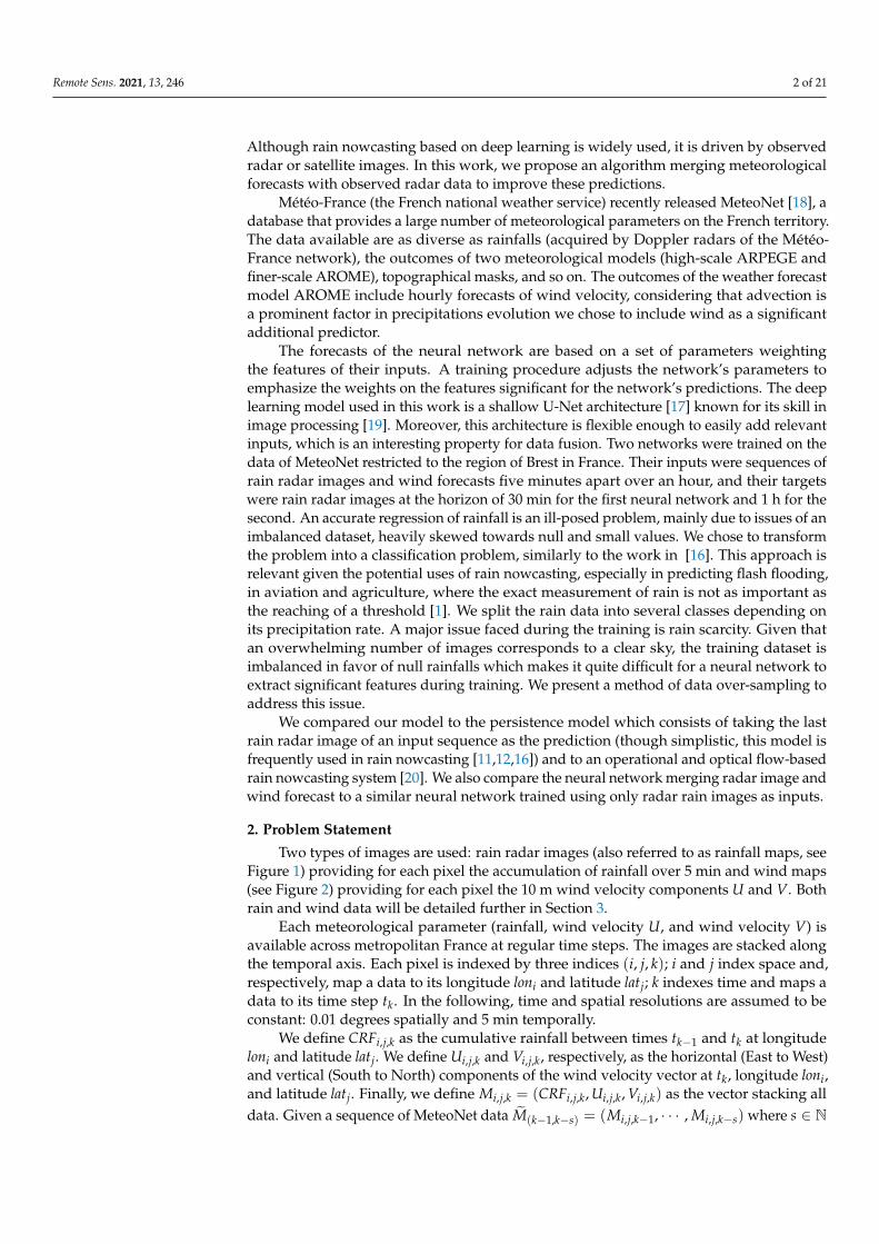
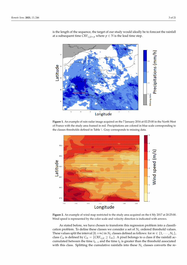
Two types of images are used: rain radar images (also referred to as rainfall maps, seeFigure 1) providing for each pixel the accumulation of rainfall over 5 min and wind maps(see Figure 2) providing for each pixel the 10 m wind velocity components U and V. Bothrain and wind data will be detailed further in Section 3.

Each meteorological parameter (rainfall, wind velocity U, and wind velocity V) isavailable across metropolitan France at regular time steps. The images are stacked alongthe temporal axis. Each pixel is indexed by three indices (i, j, k); i and j index space and,respectively, map a data to its longitude loni and latitude latj; k indexes time and maps adata to its time step tk. In the following, time and spatial resolutions are assumed to beconstant: 0.01 degrees spatially and 5 min temporally.

We define CRFi,j,k as the cumulative rainfall between times tk−1 and tk at longitudeloni and latitude latj. We define Ui,j,k and Vi,j,k, respectively, as the horizontal (East to West)and vertical (South to North) components of the wind velocity vector at tk, longitude loni,and latitude latj. Finally, we define Mi,j,k = (CRFi,j,k, Ui,j,k, Vi,j,k) as the vector stacking alldata. Given a sequence of MeteoNet data M(k−1,k−s) = (Mi,j,k−1, · · · , Mi,j,k−s) where s ∈ N

Remote Sens. 2021, 13, 246 3 of 21

is the length of the sequence, the target of our study would ideally be to forecast the rainfallat a subsequent time CRFi,j,k+p where p ∈ N is the lead time step.

Figure 1. An example of rain radar image acquired on the 7 January 2016 at 02:25:00 in the North Westof France with the study area framed in red. Precipitations are colored in blue scale corresponding tothe classes thresholds defined in Table 1. Gray corresponds to missing data.

Figure 2. An example of wind map restricted to the study area acquired on the 6 My 2017 at 20:25:00.Wind speed is represented by the color scale and velocity direction is indicated with arrows.

As stated before, we have chosen to transform this regression problem into a classifi-cation problem. To define these classes we consider a set of NL ordered threshold values.These values split the interval [0;+∞) in NL classes defined as follows: for m ∈ 1, · · · , NL,class Cm is defined by Cm = CRFi,j,k ≥ Lm. A pixel belongs to a class if the rainfall ac-cumulated between the time tk−1 and the time tk is greater than the threshold associatedwith this class. Splitting the cumulative rainfalls into these NL classes converts the re-

Remote Sens. 2021, 13, 246 4 of 21

gression task from directly predicting CRFi,j,k+p to determining to which classes CRFi,j,k+pbelongs to. The classes are embedded, i.e., if a CRFi,j,k belongs to Cm, then it also belongs toCn, ∀1 ≤ n < m. Therefore, a prediction can belong to several classes. This type of problemwith embedded classes is formalized as multi-label classification problem, and it is oftentransformed into NL binary classification problems using the binary relevance method [21].Therefore, we will train NL binary classifiers; classifier m determines the probability thatCRFi,j,k+p exceeds the threshold Lm.

Table 1. Summary of classes definition and distribution.

m Qualitative Label Class Definition Pixels by Class (%) Images ContainingClass m (%)

1 Very light rain and higher CRF ≥ 0.1 mm/h 7.4% 61%

2 Continuous light rain and higher CRF ≥ 1 mm/h 2.9% 43%

3 Moderate rain and higher CRF ≥ 2.5 mm/h 1.2% 34%

Knowing M(k−1,k−s), the classifier m will estimate the probability Pmi,j,k that the cumu-

lative rainfall CRFi,j,k+p belongs to Cm:

Pmi,j,k = Pm(CRFi,j,k+p ∈ Cm | M(k−1,k−s)) = Pm(CRFi,j,k+p ≥ Lm | M(k−1,k−s)) (1)

with Pmi,j,k ∈ [0, 1] reaching 1 if CRFi,j,k+p surely belongs to class Cm. Ultimately, all values

in the sequence of probabilities (Pmi,j,k)m∈1,··· ,NL that are above 0.5 mark that data as

belonging to Cm. When no classifier satisfies Pmi,j,k ≥ 0.5, no rain is predicted.

3. Data

MeteoNet [18] is a Météo-France project gathering meteorological data on the Frenchterritory. Every data type available spans from 2016 to 2018 on two areas of 500 km × 500 kmeach, framing the northwest and southeast parts of the French metropolis. This paperfocuses on rain radar and wind data in the northwest area.

3.1. Rain Data3.1.1. Presentation of the Meteonet Rain Radar Images and Definition of the Study Area

The rain data in the northwest part of France provided by MeteoNet is the cumulativerainfall over time steps of 5 min. The acquisition of the data is made using Météo-FranceDoppler radar network: each radar scans the sky to build a 3D reflectivity map, the differentmaps are then checked by Météo-France to remove meteorological artifacts and to obtainMeteoNet rainfall data. The spatial resolution of the data is 0.01 degrees (roughly 1 km ×1.2 km). More information can be found in [22] about the Météo-France radar network andin [23] about the measurement of rainfall.

The data presented in MeteoNet are images of size 565× 784 pixels, each pixel’s valuebeing the CRF over 5 min. These images are often referred to as rainfall maps in this paper(see Figure 1 for an example).

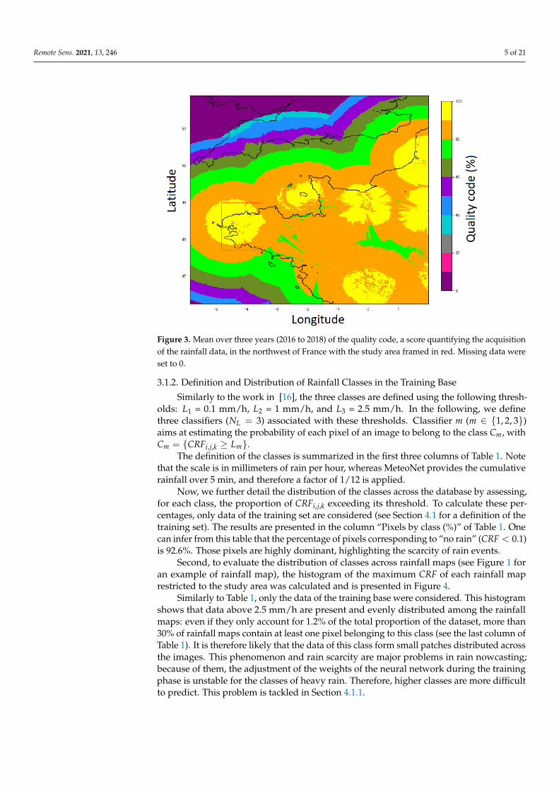
The aim is to predict the rainfall at the scale of a French department hence the studyarea has been restricted to 128× 128 pixels (roughly 100 km × 150 km). However, as thequality of the acquisition is not uniform across the territory, MeteoNet provides a rain radarquality code data (spanning from 0% to 100%) to quantify the quality of the acquisition oneach pixel (see Figure 3). The department of Finistère is mainly inland and has an overallquality code score over 80% hence the study area has been centered on the city of Brest.

Remote Sens. 2021, 13, 246 5 of 21

Figure 3. Mean over three years (2016 to 2018) of the quality code, a score quantifying the acquisitionof the rainfall data, in the northwest of France with the study area framed in red. Missing data wereset to 0.

3.1.2. Definition and Distribution of Rainfall Classes in the Training Base

Similarly to the work in [16], the three classes are defined using the following thresh-olds: L1 = 0.1 mm/h, L2 = 1 mm/h, and L3 = 2.5 mm/h. In the following, we definethree classifiers (NL = 3) associated with these thresholds. Classifier m (m ∈ 1, 2, 3)aims at estimating the probability of each pixel of an image to belong to the class Cm, withCm = CRFi,j,k ≥ Lm.

The definition of the classes is summarized in the first three columns of Table 1. Notethat the scale is in millimeters of rain per hour, whereas MeteoNet provides the cumulativerainfall over 5 min, and therefore a factor of 1/12 is applied.

Now, we further detail the distribution of the classes across the database by assessing,for each class, the proportion of CRFi,j,k exceeding its threshold. To calculate these per-centages, only data of the training set are considered (see Section 4.1 for a definition of thetraining set). The results are presented in the column “Pixels by class (%)” of Table 1. Onecan infer from this table that the percentage of pixels corresponding to “no rain” (CRF < 0.1)is 92.6%. Those pixels are highly dominant, highlighting the scarcity of rain events.

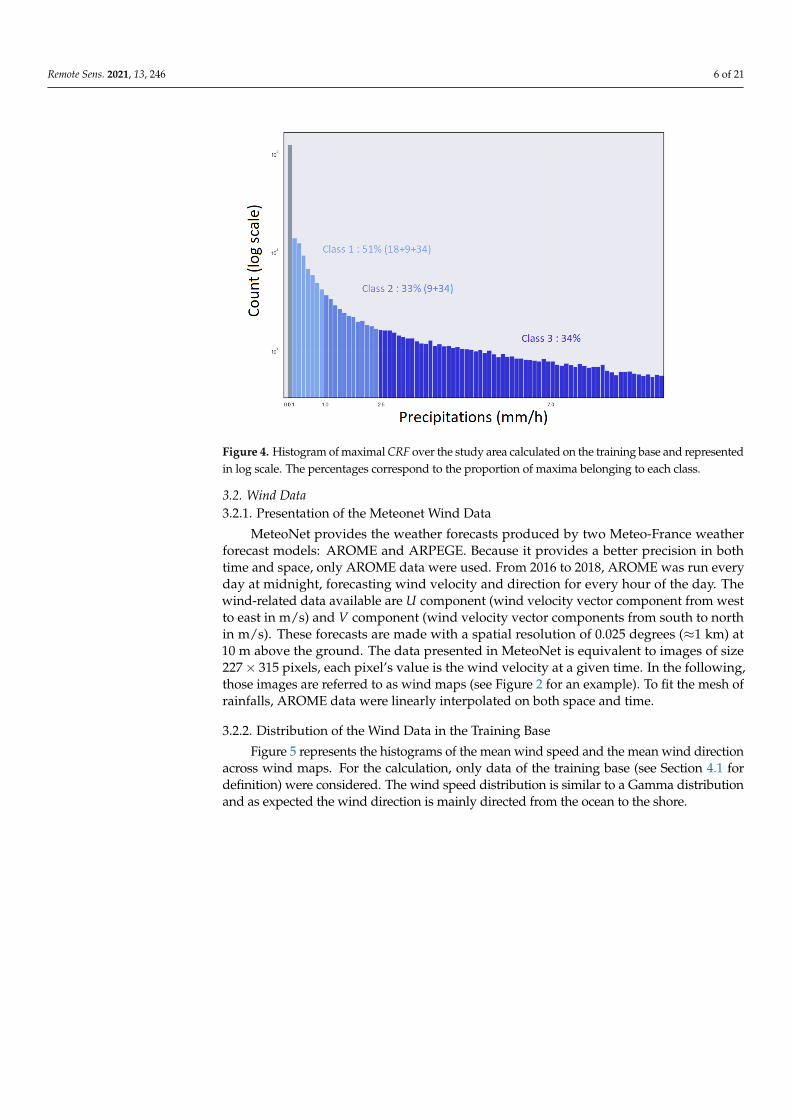
Second, to evaluate the distribution of classes across rainfall maps (see Figure 1 foran example of rainfall map), the histogram of the maximum CRF of each rainfall maprestricted to the study area was calculated and is presented in Figure 4.

Similarly to Table 1, only the data of the training base were considered. This histogramshows that data above 2.5 mm/h are present and evenly distributed among the rainfallmaps: even if they only account for 1.2% of the total proportion of the dataset, more than30% of rainfall maps contain at least one pixel belonging to this class (see the last column ofTable 1). It is therefore likely that the data of this class form small patches distributed acrossthe images. This phenomenon and rain scarcity are major problems in rain nowcasting;because of them, the adjustment of the weights of the neural network during the trainingphase is unstable for the classes of heavy rain. Therefore, higher classes are more difficultto predict. This problem is tackled in Section 4.1.1.

Remote Sens. 2021, 13, 246 6 of 21

Figure 4. Histogram of maximal CRF over the study area calculated on the training base and representedin log scale. The percentages correspond to the proportion of maxima belonging to each class.

3.2. Wind Data3.2.1. Presentation of the Meteonet Wind Data

MeteoNet provides the weather forecasts produced by two Meteo-France weatherforecast models: AROME and ARPEGE. Because it provides a better precision in bothtime and space, only AROME data were used. From 2016 to 2018, AROME was run everyday at midnight, forecasting wind velocity and direction for every hour of the day. Thewind-related data available are U component (wind velocity vector component from westto east in m/s) and V component (wind velocity vector components from south to northin m/s). These forecasts are made with a spatial resolution of 0.025 degrees (≈1 km) at10 m above the ground. The data presented in MeteoNet is equivalent to images of size227× 315 pixels, each pixel’s value is the wind velocity at a given time. In the following,those images are referred to as wind maps (see Figure 2 for an example). To fit the mesh ofrainfalls, AROME data were linearly interpolated on both space and time.

3.2.2. Distribution of the Wind Data in the Training Base

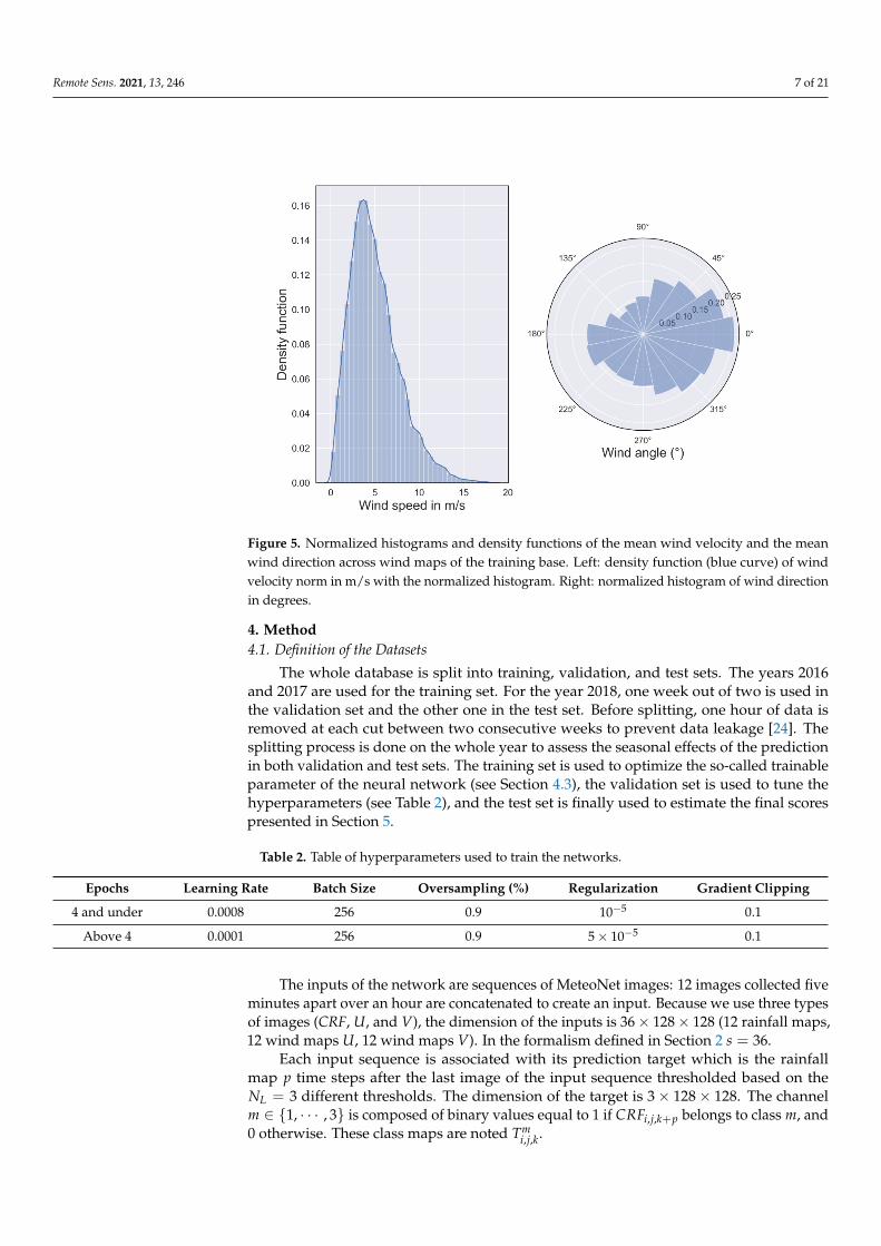
Figure 5 represents the histograms of the mean wind speed and the mean wind directionacross wind maps. For the calculation, only data of the training base (see Section 4.1 fordefinition) were considered. The wind speed distribution is similar to a Gamma distributionand as expected the wind direction is mainly directed from the ocean to the shore.

Remote Sens. 2021, 13, 246 7 of 21

Figure 5. Normalized histograms and density functions of the mean wind velocity and the meanwind direction across wind maps of the training base. Left: density function (blue curve) of windvelocity norm in m/s with the normalized histogram. Right: normalized histogram of wind directionin degrees.

4. Method4.1. Definition of the Datasets

The whole database is split into training, validation, and test sets. The years 2016and 2017 are used for the training set. For the year 2018, one week out of two is used inthe validation set and the other one in the test set. Before splitting, one hour of data isremoved at each cut between two consecutive weeks to prevent data leakage [24]. Thesplitting process is done on the whole year to assess the seasonal effects of the predictionin both validation and test sets. The training set is used to optimize the so-called trainableparameter of the neural network (see Section 4.3), the validation set is used to tune thehyperparameters (see Table 2), and the test set is finally used to estimate the final scorespresented in Section 5.

Table 2. Table of hyperparameters used to train the networks.

Epochs Learning Rate Batch Size Oversampling (%) Regularization Gradient Clipping

4 and under 0.0008 256 0.9 10−5 0.1

Above 4 0.0001 256 0.9 5× 10−5 0.1

The inputs of the network are sequences of MeteoNet images: 12 images collected fiveminutes apart over an hour are concatenated to create an input. Because we use three typesof images (CRF, U, and V), the dimension of the inputs is 36× 128× 128 (12 rainfall maps,12 wind maps U, 12 wind maps V). In the formalism defined in Section 2 s = 36.

Each input sequence is associated with its prediction target which is the rainfallmap p time steps after the last image of the input sequence thresholded based on theNL = 3 different thresholds. The dimension of the target is 3× 128× 128. The channelm ∈ 1, · · · , 3 is composed of binary values equal to 1 if CRFi,j,k+p belongs to class m, and0 otherwise. These class maps are noted Tm

i,j,k.

Remote Sens. 2021, 13, 246 8 of 21

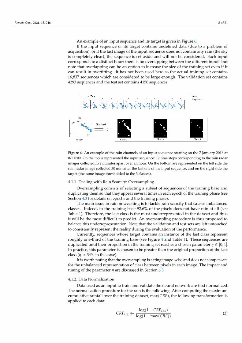
An example of an input sequence and its target is given in Figure 6.If the input sequence or its target contains undefined data (due to a problem of

acquisition), or if the last image of the input sequence does not contain any rain (the skyis completely clear), the sequence is set aside and will not be considered. Each inputcorresponds to a distinct hour: there is no overlapping between the different inputs butnote that overlapping can be an option to increase the size of the training set even if itcan result in overfitting. It has not been used here as the actual training set contains16,837 sequences which are considered to be large enough. The validation set contains4293 sequences and the test set contains 4150 sequences.

Figure 6. An example of the rain channels of an input sequence starting on the 7 January 2016 at07:00:00. On the top is represented the input sequence: 12 time steps corresponding to the rain radarimages collected five minutes apart over an hour. On the bottom are represented on the left side therain radar image collected 30 min after the last one of the input sequence, and on the right side thetarget (the same image thresholded to the 3 classes).

4.1.1. Dealing with Rain Scarcity: Oversampling

Oversampling consists of selecting a subset of sequences of the training base andduplicating them so that they appear several times in each epoch of the training phase (seeSection 4.3 for details on epochs and the training phase).

The main issue in rain nowcasting is to tackle rain scarcity that causes imbalancedclasses. Indeed, in the training base 92.6% of the pixels does not have rain at all (seeTable 1). Therefore, the last class is the most underrepresented in the dataset and thusit will be the most difficult to predict. An oversampling procedure is thus proposed tobalance this underrepresentation. Note that the validation and test sets are left untouchedto consistently represent the reality during the evaluation of the performance.

Currently, sequences whose target contains an instance of the last class representroughly one-third of the training base (see Figure 4 and Table 1). These sequences areduplicated until their proportion in the training set reaches a chosen parameter η ∈ [0, 1].In practice, this parameter is chosen to be greater than the original proportion of the lastclass (η > 34% in this case).

It is worth noting that the oversampling is acting image-wise and does not compensatefor the unbalanced representation of class between pixels in each image. The impact andtuning of the parameter η are discussed in Section 6.3.

4.1.2. Data Normalization

Data used as an input to train and validate the neural network are first normalized.The normalization procedure for the rain is the following. After computing the maximumcumulative rainfall over the training dataset, max(CRF), the following transformation isapplied to each data:

CRFi,j,k ←log(1 + CRFi,j,k)

log(1 + max(CRF))(2)

Remote Sens. 2021, 13, 246 9 of 21

This invertible normalization function brings the dataset into the [0, 1] range whilespreading out the values closest to 0.

As for wind data, considering that U and V follow a Gaussian distribution, with µand σ, respectively, the mean and the standard deviation of wind over the overall trainingset, we apply

Ui,j,k ←Ui,j,k − µU

σU(3)

Vi,j,k ←Vi,j,k − µV

σV(4)

4.2. Network Architecture

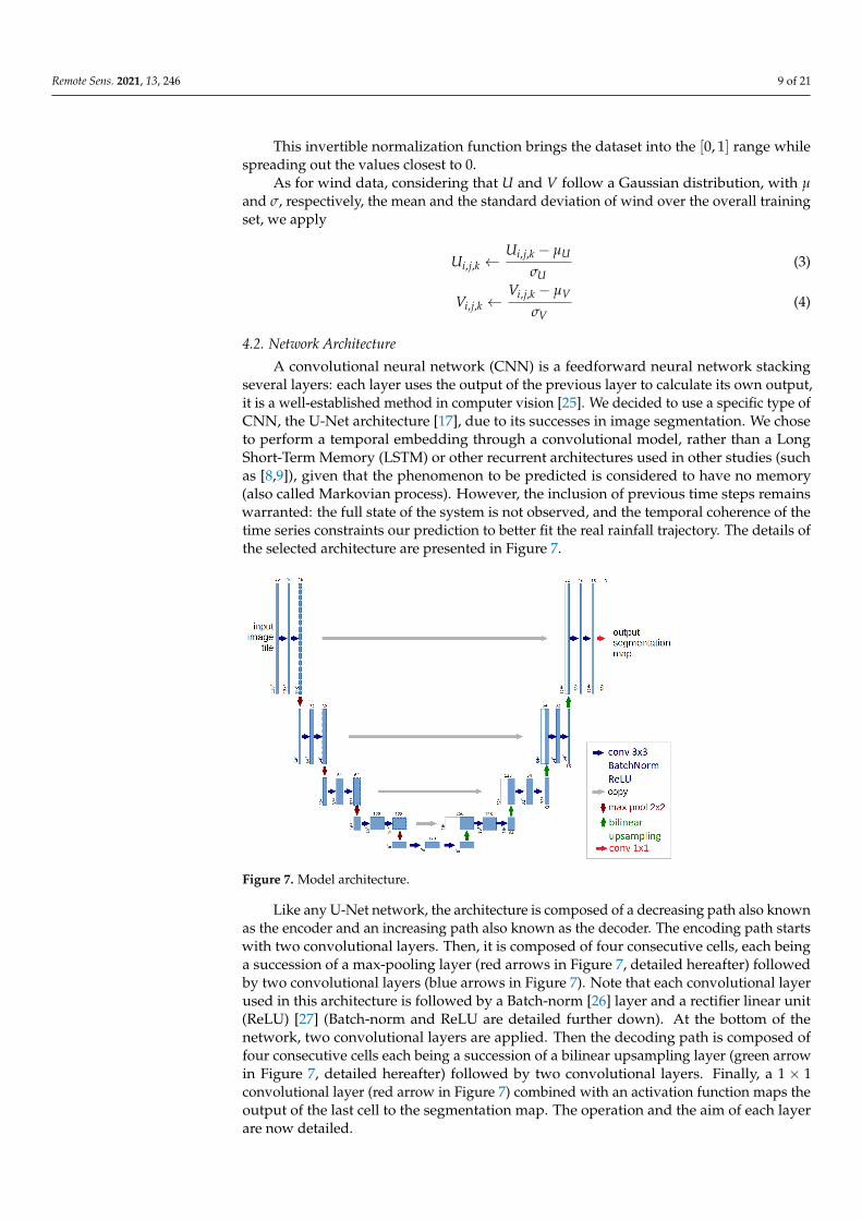
A convolutional neural network (CNN) is a feedforward neural network stackingseveral layers: each layer uses the output of the previous layer to calculate its own output,it is a well-established method in computer vision [25]. We decided to use a specific type ofCNN, the U-Net architecture [17], due to its successes in image segmentation. We choseto perform a temporal embedding through a convolutional model, rather than a LongShort-Term Memory (LSTM) or other recurrent architectures used in other studies (suchas [8,9]), given that the phenomenon to be predicted is considered to have no memory(also called Markovian process). However, the inclusion of previous time steps remainswarranted: the full state of the system is not observed, and the temporal coherence of thetime series constraints our prediction to better fit the real rainfall trajectory. The details ofthe selected architecture are presented in Figure 7.

Figure 7. Model architecture.

Like any U-Net network, the architecture is composed of a decreasing path also knownas the encoder and an increasing path also known as the decoder. The encoding path startswith two convolutional layers. Then, it is composed of four consecutive cells, each beinga succession of a max-pooling layer (red arrows in Figure 7, detailed hereafter) followedby two convolutional layers (blue arrows in Figure 7). Note that each convolutional layerused in this architecture is followed by a Batch-norm [26] layer and a rectifier linear unit(ReLU) [27] (Batch-norm and ReLU are detailed further down). At the bottom of thenetwork, two convolutional layers are applied. Then the decoding path is composed offour consecutive cells each being a succession of a bilinear upsampling layer (green arrowin Figure 7, detailed hereafter) followed by two convolutional layers. Finally, a 1 × 1convolutional layer (red arrow in Figure 7) combined with an activation function maps theoutput of the last cell to the segmentation map. The operation and the aim of each layerare now detailed.

Remote Sens. 2021, 13, 246 10 of 21

4.2.1. Convolutional Layers

Convolutional layers perform a convolution by a kernel of 3× 3, a padding of 1 is usedto preserve the input size. The parameters of the convolutions are to be learned during thetraining phase. Each convolutional layer in this architecture is followed by a Batch-normand a ReLU layer.

A Batch-norm layer re-centers and re-scales its inputs to ensure that the mean is closeto 0 and the standard deviation is close to 1. Batch-norm helps the network to train fasterand to be more stable [26]. For an input batch Batch, the output is y = E[Batch]√

V[Batch]+εγ + β,

where γ and β are trainable parameters, E[·] is the average, and V[·] is the variance of theinput batch. In our architecture, the constant ε is set to 10−5.

A ReLU layer, standing for rectifier linear unit, applies the following nonlinear func-tion f : x ∈ R 7→ max(0, x). Adding nonlinearities enables the network to model non-linearrelations between the input and output images.

4.2.2. Image Sample

To upsample or subsample the images, two types of layers are considered.The Max-pooling layer is used to reduce the image feature sizes in the encoding part. It

browses the input with a 2× 2 filter and maps each patch to its maximum. It reduces the sizeof the image by a factor between each level of the encoding path. It also contributes to preventoverfitting by reducing the number of parameters to be optimized during the training.

The bilinear upsampling layer is used to increase the image feature sizes in thedecoding part. It performs a bilinear interpolation of the input resulting in the size of theoutput being twice the one of the input.

4.2.3. Skip Connections

Skip connections (in gray in Figure 7) are the trademarks of the U-Net architecture.The output of an encoding cell is stacked to the output of a decoding cell of the samedimension and the stacking is used as input for the next decoding cell. Therefore, skipconnections spread some information from the encoding path to the decoding path andthus help to prevent the vanishing gradient problem [28] and allow to prevent some smallscale features in the encoding path.

4.2.4. Output Layer

The final layer is a convolutional layer with a 1× 1 kernel. The dimension of its outputis 3× 128× 128, there is one channel for each class. For a given point we define the scoresm as the output of channel m (m ∈ 1, 2, 3). This output sm is then transformed using thesigmoid function to obtain the probability Pm

i,j,k:

Pmi,j,k =

11 + esm

(5)

where Pmi,j,k is defined in Section 2. Note that, following the definition of the classes in

Table 1, one point can belong to several classes.Finally, the output is said to belong to the class m if Pm

i,j,k ≥12 .

4.3. Network Training

We call θ the vector of length Nθ containing the trainable parameters (also nameweights) that are to be determined through the training procedure. The training processconsists of splitting the training dataset into several batches, inputting successively thebatches into the network, calculating the distance between the predictions and the targetsvia a loss function, and finally, based on the calculated loss, updating the network weightsusing an optimization algorithm. The training procedure is repeated during several epochs(one epoch being achieved when the entire training set has gone through the network) andaims at minimizing the loss function.

Remote Sens. 2021, 13, 246 11 of 21

For a given input sequence M(k−1,k−s), we define the binary cross-entropy loss func-tion [29] Loss comparing the output Pm

i,j,k to its target Tmi,j,k:

Loss(θ) = − 1NL

NL

∑m=1

(Tm

i,j,k log(Pmi,j,k) + (1− Tm

i,j,k) log(1− Pmi,j,k)

)(6)

This loss is averaged across the batch, then a regularization term is added:

Regularization(θ) =δ

Nθ

Nθ

∑l=1

θ2l (7)

The loss function minimizes the discrepancy between the targeted value and thepredicted value, and the second term is a square regularization (also called Tikhonovor `2-regularization) aiming at preventing overfitting and distributing the weights moreevenly. The importance of this regularization in the training process is weighted by thefactor δ.

The optimization algorithm used is Adam [30] (standing for Adaptive Moment Esti-mation), which is a stochastic gradient descent algorithm. The recommended parametersare used: β1 = 0.9, β2 = 0.999 and ε = 10−8.

Moreover, to prevent an exploding gradient, the gradient clipping technique is used.it consists of re-scaling the gradient if it becomes too large to keep it small.

The training procedure for the two neural networks is the following.

• The network whose horizon time is 30 min is trained on 20 epochs. Initially, thelearning rate is set to 0.0008 and after 4 epochs it is reduced to 0.0001. After epoch 13,the validation F1-score (the F1-score is defined in Section 4.4) is not increasing. Weselected the weights optimized after epoch 13 because their F1-score are the higheston the validation set.

• The network whose horizon time is 1 h is trained on 20 epochs. Initially, the learningrate is set to 0.0008 and after 4 epochs it is reduced to 0.0001. After epoch 17, thevalidation F1-score is not increasing. We selected the weights of epoch 17 becausetheir F1-score are the highest on the validation set.

The network is particularly sensitive to hyperparameters, specifically the learningrate, the batch size, and the percentage of oversampling. The tuning of the oversamplingpercentage is detailed in Section 4.1.1). The other hyperparameters used to train our modelsare presented in Table 2.

Neural networks were implemented and trained using PyTorch 1.5.1. on a computerwith a CPU Intel(R) Xeon(R) CPU E5-2695 v4, 2.10GHz, and a GPU PNY Tesla P100 (12 GB).

For the implementation details, please refer to the code available online: some demon-stration code to train the network, the weights, and an example of usage is available on theGitLab repository ( https://github.com/VincentBouget/rain-nowcasting-with-fusion-of-rainfall-and-wind-data-article) and archived in Zenodo (https://zenodo.org/record/4284847).

4.4. Scores

Among several metrics presented in the literature [8,31], the F1-score, the Threat Score(TS), and the BIAS have been selected. The algorithm seems unable to predict the smallscales resulting in smooth borders expressing the uncertainty of the retrieval for thesefeatures. This is expected, given that, at small scales, rainfalls are usually related to otherprocesses than the advection of the rain cell (e.g., intensive convection) have been selected.As our algorithm is a multi-label classification problem, each of the NL classifiers is assessedindependently of the others. For a given input sequence M(k−1,k−s), we compare the output(Pm

i,j,k thresholded by 0.5) to its target Tmi,j,k. Because it is a binary classification, four possible

outcomes can be obtained:

Remote Sens. 2021, 13, 246 12 of 21

• True Positive TPmi,j,k when the classifier rightly predict the occurrence of an event (also

called hits).• True Negative TNm

i,j,k when the classifier rightly predict the absence of an event.• False Positive FPm

i,j,k when the classifier predicts the occurrence of an event that hasnot occurred (also called false alarm).

• False Negative FNmi,j,k when the classifier predicts the absence of an event that has

occurred (also called missed).

On the one hand, we can define the threat score and the BIAS:

TSm =

∑i,j,k

TPmi,j,k

∑i,j,k

TPmi,j,k + FPm

i,j,k + FNmi,j,k

(8)

BIASm =

∑i,j,k

TPmi,j,k + FPm

i,j,k

∑i,j,k

TPmi,j,k + FNm

i,j,k(9)

TS range from 0 to 1, where 0 is the worst possible classification and 1 is a perfectclassifier. BIAS range from 0 to +∞, 1 corresponds to a non-biased classifier. A score under1 means that the classifier underestimates the rain and a score greater than 1 means thatthe classifier overestimates the rain.

On the other hand, we can define the precision and the recall:

Precisionm =

∑i,j,k

TPmi,j,k

∑i,j,k

TPmi,j,k + FPm

i,j,k(10)

Recallm =

∑i,j,k

TPmi,j,k

∑i,j,k

TPmi,j,k + FNm

i,j,k(11)

Note that, in theory, if the classifier is predicting 0 for all the data (i.e., no rain), thePrecision is not defined because its denominator is null. Nevertheless, as the simulation is doneover all the samples of the validation or test dataset, this situation hardly occurs in practice.

Based on those definitions, the F1-score, F1m for the classifier m, can be defined as theharmonic mean between the precision and the recall as

F1m = 2Precisionm × RecallmPrecisionm + Recallm

(12)

Precision, Recall, and F1-score range from 0 to 1, where 0 is the worst possible classifi-cation and 1 is a perfect classifier.

All these scores will be computed on the test dataset to assess our models’ perfor-mance.

4.5. Baseline

We briefly present the optical flow method used in Section 5 as a baseline. If I is asequence of images (in our case, a succession of CRF maps), the optical flow assumes theadvection of I by velocity W = (U, V) at pixel (x, y) and time t:

∂I∂t(x, y, t) +∇I(x, y, t)TW(x, y, t) = 0 (13)

Remote Sens. 2021, 13, 246 13 of 21

where ∇ is the gradient operator and T the transpose operator, i.e., ∇IT =(

∂I∂x

∂I∂y

).

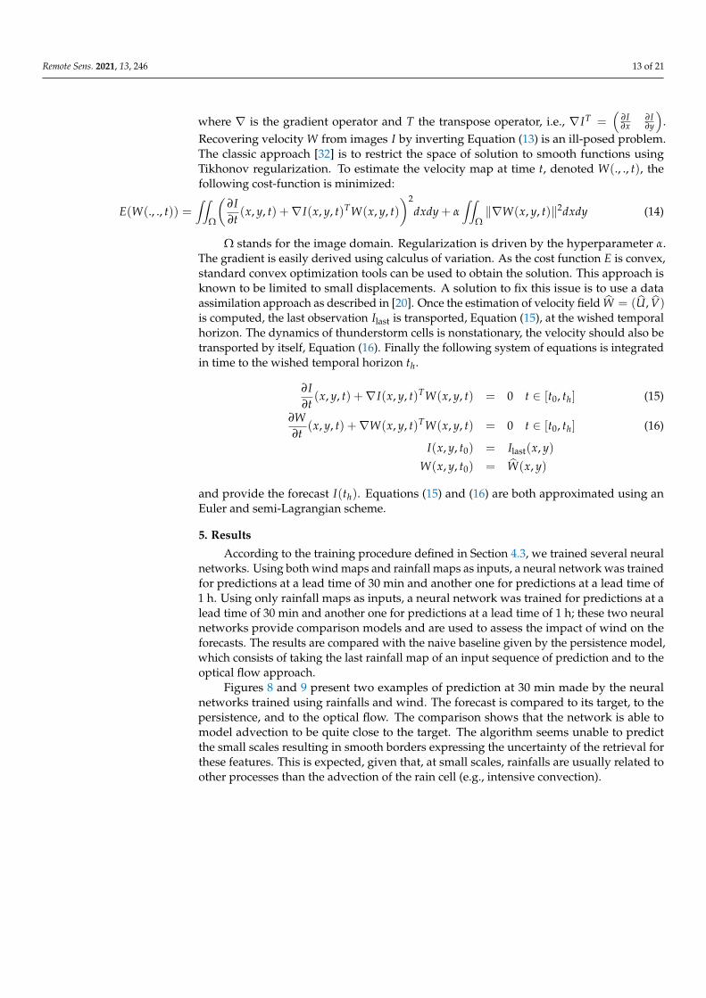
Recovering velocity W from images I by inverting Equation (13) is an ill-posed problem.The classic approach [32] is to restrict the space of solution to smooth functions usingTikhonov regularization. To estimate the velocity map at time t, denoted W(., ., t), thefollowing cost-function is minimized:

E(W(., ., t)) =∫∫

Ω

(∂I∂t(x, y, t) +∇I(x, y, t)TW(x, y, t)

)2dxdy + α

∫∫Ω‖∇W(x, y, t)‖2dxdy (14)

Ω stands for the image domain. Regularization is driven by the hyperparameter α.The gradient is easily derived using calculus of variation. As the cost function E is convex,standard convex optimization tools can be used to obtain the solution. This approach isknown to be limited to small displacements. A solution to fix this issue is to use a dataassimilation approach as described in [20]. Once the estimation of velocity field W = (U, V)is computed, the last observation Ilast is transported, Equation (15), at the wished temporalhorizon. The dynamics of thunderstorm cells is nonstationary, the velocity should also betransported by itself, Equation (16). Finally the following system of equations is integratedin time to the wished temporal horizon th.

∂I∂t(x, y, t) +∇I(x, y, t)TW(x, y, t) = 0 t ∈ [t0, th] (15)

∂W∂t

(x, y, t) +∇W(x, y, t)TW(x, y, t) = 0 t ∈ [t0, th] (16)

I(x, y, t0) = Ilast(x, y)

W(x, y, t0) = W(x, y)

and provide the forecast I(th). Equations (15) and (16) are both approximated using anEuler and semi-Lagrangian scheme.

5. Results

According to the training procedure defined in Section 4.3, we trained several neuralnetworks. Using both wind maps and rainfall maps as inputs, a neural network was trainedfor predictions at a lead time of 30 min and another one for predictions at a lead time of1 h. Using only rainfall maps as inputs, a neural network was trained for predictions at alead time of 30 min and another one for predictions at a lead time of 1 h; these two neuralnetworks provide comparison models and are used to assess the impact of wind on theforecasts. The results are compared with the naive baseline given by the persistence model,which consists of taking the last rainfall map of an input sequence of prediction and to theoptical flow approach.

Figures 8 and 9 present two examples of prediction at 30 min made by the neuralnetworks trained using rainfalls and wind. The forecast is compared to its target, to thepersistence, and to the optical flow. The comparison shows that the network is able tomodel advection to be quite close to the target. The algorithm seems unable to predictthe small scales resulting in smooth borders expressing the uncertainty of the retrieval forthese features. This is expected, given that, at small scales, rainfalls are usually related toother processes than the advection of the rain cell (e.g., intensive convection).

Remote Sens. 2021, 13, 246 14 of 21

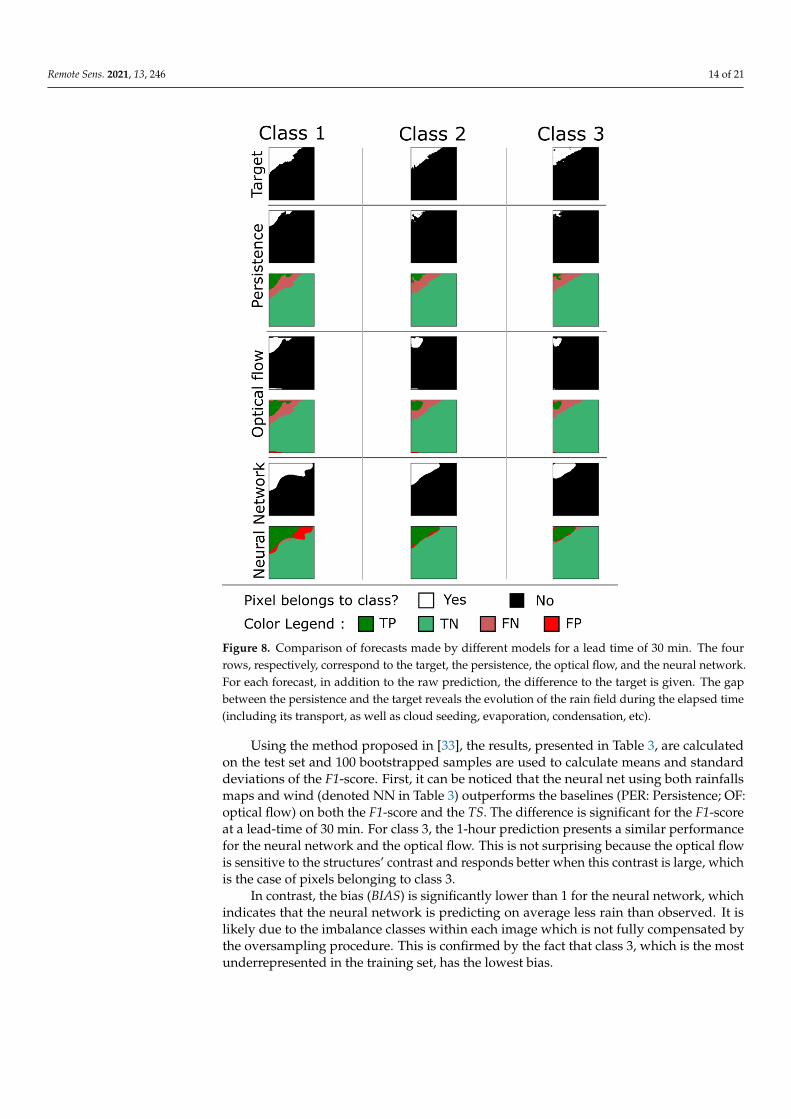
Figure 8. Comparison of forecasts made by different models for a lead time of 30 min. The fourrows, respectively, correspond to the target, the persistence, the optical flow, and the neural network.For each forecast, in addition to the raw prediction, the difference to the target is given. The gapbetween the persistence and the target reveals the evolution of the rain field during the elapsed time(including its transport, as well as cloud seeding, evaporation, condensation, etc).

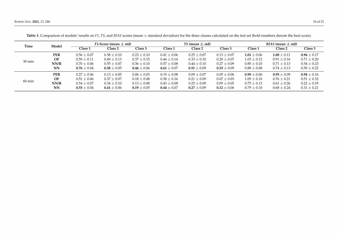
Using the method proposed in [33], the results, presented in Table 3, are calculatedon the test set and 100 bootstrapped samples are used to calculate means and standarddeviations of the F1-score. First, it can be noticed that the neural net using both rainfallsmaps and wind (denoted NN in Table 3) outperforms the baselines (PER: Persistence; OF:optical flow) on both the F1-score and the TS. The difference is significant for the F1-scoreat a lead-time of 30 min. For class 3, the 1-hour prediction presents a similar performancefor the neural network and the optical flow. This is not surprising because the optical flowis sensitive to the structures’ contrast and responds better when this contrast is large, whichis the case of pixels belonging to class 3.

In contrast, the bias (BIAS) is significantly lower than 1 for the neural network, whichindicates that the neural network is predicting on average less rain than observed. It islikely due to the imbalance classes within each image which is not fully compensated bythe oversampling procedure. This is confirmed by the fact that class 3, which is the mostunderrepresented in the training set, has the lowest bias.

Remote Sens. 2021, 13, 246 15 of 21

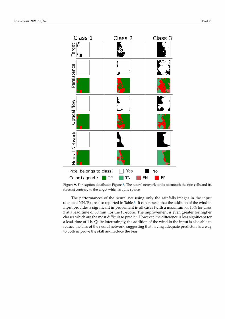
Figure 9. For caption details see Figure 8. The neural network tends to smooth the rain cells and itsforecast contrary to the target which is quite sparse.

The performances of the neural net using only the rainfalls images in the input(denoted NN/R) are also reported in Table 3. It can be seen that the addition of the wind ininput provides a significant improvement in all cases (with a maximum of 10% for class3 at a lead time of 30 min) for the F1-score. The improvement is even greater for higherclasses which are the most difficult to predict. However, the difference is less significant fora lead-time of 1 h. Quite interestingly, the addition of the wind in the input is also able toreduce the bias of the neural network, suggesting that having adequate predictors is a wayto both improve the skill and reduce the bias.

Remote Sens. 2021, 13, 246 16 of 21

Table 3. Comparison of models’ results on F1, TS, and BIAS scores (mean ± standard deviation) for the three classes calculated on the test set (bold numbers denote the best score).

Time Model F1-Score (mean ± std) TS (mean ± std) BIAS (mean ± std)Class 1 Class 2 Class 3 Class 1 Class 2 Class 3 Class 1 Class 2 Class 3

30 min

PER 0.56 ± 0.07 0.38 ± 0.10 0.23 ± 0.10 0.41 ± 0.06 0.25 ± 0.07 0.13 ± 0.07 1.01 ± 0.06 1.00 ± 0.11 0.96 ± 0.17OF 0.59 ± 0.11 0.49 ± 0.13 0.37 ± 0.15 0.44 ± 0.14 0.33 ± 0.10 0.20 ± 0.07 1.03 ± 0.12 0.91 ± 0.16 0.71 ± 0.20

NN/R 0.70 ± 0.06 0.55 ± 0.07 0.36 ± 0.10 0.57 ± 0.08 0.44 ± 0.10 0.27 ± 0.09 0.85 ± 0.10 0.71 ± 0.13 0.54 ± 0.23NN 0.76 ± 0.04 0.58 ± 0.05 0.46 ± 0.06 0.61 ± 0.07 0.51 ± 0.09 0.35 ± 0.09 0.88 ± 0.08 0.74 ± 0.13 0.59 ± 0.22

60 min

PER 0.27 ± 0.06 0.13 ± 0.05 0.06 ± 0.03 0.19 ± 0.08 0.09 ± 0.07 0.05 ± 0.06 0.99 ± 0.06 0.95 ± 0.09 0.94 ± 0.16OF 0.51 ± 0.06 0.37 ± 0.07 0.18 ± 0.08 0.38 ± 0.16 0.21 ± 0.09 0.07 ± 0.03 1.09 ± 0.10 0.76 ± 0.21 0.51 ± 0.32

NN/R 0.54 ± 0.07 0.34 ± 0.10 0.13 ± 0.08 0.43 ± 0.08 0.25 ± 0.09 0.09 ± 0.05 0.75 ± 0.13 0.61 ± 0.26 0.22 ± 0.19NN 0.55 ± 0.04 0.41 ± 0.06 0.19 ± 0.05 0.44 ± 0.07 0.27 ± 0.09 0.12 ± 0.06 0.79 ± 0.10 0.68 ± 0.24 0.31 ± 0.21

Remote Sens. 2021, 13, 246 17 of 21

6. Discussion6.1. Choice of Input Data

One objective of this work was to show that adding relevant data as input could causea significant improvement in nowcasting. We expect that the choice of input data can havean incidence of the improvement of the prediction skill. In this work, the 10 m wind wasconsidered as a proxy for all the factors that could potentially influence the rain cloudformation, motion, and deformation. In particular, we did not choose the wind as the cloudlevel given the huge uncertainty of the cloud height and thickness [34]. It has also beenchosen because it is a standard product distributed in operational products and therefore itis reasonable to assume that we can estimate this parameter in a near-real-time context thatcould be a future application of our approach. Limiting the input factors to the wind and theradar images will limit the predictability of the algorithm. In particular, we cannot predict theformation of clouds. In future work, it could worth investigating other parameters such as2 m air temperature, surface geopotential, or vertical profiles of geopotential and wind speedsthat could help to predict other mechanisms leading to precipitations.

6.2. Dependency of Classes

Following the class definition in Section 2, the classes are not independent, giventhat a point belonging to Cm would imply that it also belongs to Cn, ∀1 ≤ n < m. Thisconstraint was not explicitly imposed on the classifier, and as such it could violate thisprinciple. In practice, we have not observed this phenomenon. Alternative modeling basedon the classifier chains method [35] would take this drawback into account.

6.3. Tuning the Oversampling Parameter

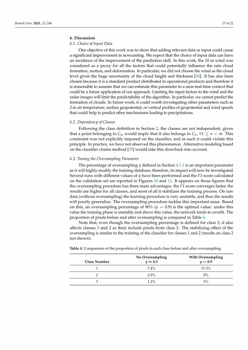
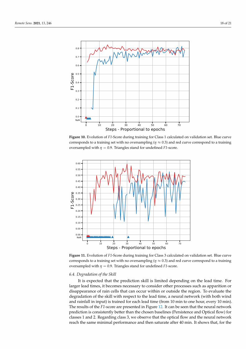
The percentage of oversampling η defined in Section 4.1.1 is an important parameteras it will highly modify the training database; therefore, its impact will now be investigated.Several runs with different values of η have been performed and the F1-score calculatedon the validation set are reported in Figures 10 and 11. It appears on those figures thatthe oversampling procedure has three main advantages: the F1-score converges faster, theresults are higher for all classes, and most of all it stabilizes the training process. On rawdata (without oversampling) the learning procedure is very unstable, and thus the resultswill poorly generalize. The oversampling procedure tackles this important issue. Basedon this, an oversampling percentage of 90% (η = 0.9) is the optimal value: under thisvalue the training phase is unstable and above this value, the network tends to overfit. Theproportion of pixels before and after oversampling is compared in Table 4.

Note that, even though the oversampling percentage is defined for class 3, it alsoaffects classes 1 and 2 as their include pixels from class 3. The stabilizing effect of theoversampling is similar to the training of the classifier for classes 1 and 2 (results on class 2not shown).

Table 4. Comparison of the proportion of pixels in each class before and after oversampling.

No Oversampling With OversamplingClass Number η ≈ 0.3 η = 0.9

1 7.4% 17.3%

2 2.9% 8%

3 1.2% 3%

Remote Sens. 2021, 13, 246 18 of 21

0 10 20 30 40 50 60 70Steps - Proportional to epochs

0.0

0.1

0.2

0.3

0.4

0.5

0.6

0.7

0.8

F1-S

core

NaN

Figure 10. Evolution of F1-Score during training for Class 1 calculated on validation set. Blue curvecorresponds to a training set with no oversampling (η ≈ 0.3) and red curve correspond to a trainingoversampled with η = 0.9. Triangles stand for undefined F1-score.

0 10 20 30 40 50 60 70

Steps - Proportional to epochs

0.00

0.05

0.10

0.15

0.20

0.25

0.30

0.35

0.40

0.45

0.50

0.55

0.60

F1-S

core

NaN

Figure 11. Evolution of F1-Score during training for Class 3 calculated on validation set. Blue curvecorresponds to a training set with no oversampling (η ≈ 0.3) and red curve correspond to a trainingoversampled with η = 0.9. Triangles stand for undefined F1-score.

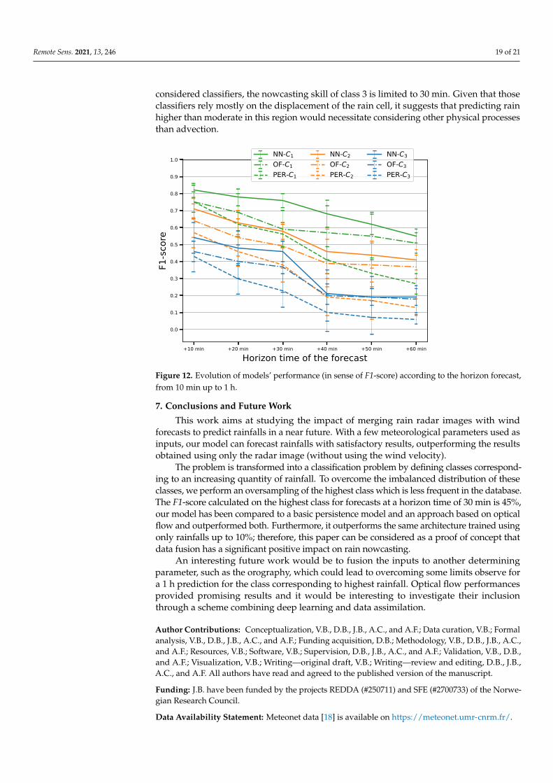
6.4. Degradation of the Skill

It is expected that the prediction skill is limited depending on the lead time. Forlarger lead times, it becomes necessary to consider other processes such as apparition ordisappearance of rain cells that can occur within or outside the region. To evaluate thedegradation of the skill with respect to the lead time, a neural network (with both windand rainfall in input) is trained for each lead time (from 10 min to one hour, every 10 min).The results of the F1-score are presented in Figure 12. It can be seen that the neural networkprediction is consistently better than the chosen baselines (Persistence and Optical flow) forclasses 1 and 2. Regarding class 3, we observe that the optical flow and the neural networkreach the same minimal performance and then saturate after 40 min. It shows that, for the

Remote Sens. 2021, 13, 246 19 of 21

considered classifiers, the nowcasting skill of class 3 is limited to 30 min. Given that thoseclassifiers rely mostly on the displacement of the rain cell, it suggests that predicting rainhigher than moderate in this region would necessitate considering other physical processesthan advection.

+10 min +20 min +30 min +40 min +50 min +60 min

Horizon time of the forecast

0.0

0.1

0.2

0.3

0.4

0.5

0.6

0.7

0.8

0.9

1.0F1

-sco

reNN-C1OF-C1PER-C1

NN-C2OF-C2PER-C2

NN-C3OF-C3PER-C3

Figure 12. Evolution of models’ performance (in sense of F1-score) according to the horizon forecast,from 10 min up to 1 h.

7. Conclusions and Future Work

This work aims at studying the impact of merging rain radar images with windforecasts to predict rainfalls in a near future. With a few meteorological parameters used asinputs, our model can forecast rainfalls with satisfactory results, outperforming the resultsobtained using only the radar image (without using the wind velocity).

The problem is transformed into a classification problem by defining classes correspond-ing to an increasing quantity of rainfall. To overcome the imbalanced distribution of theseclasses, we perform an oversampling of the highest class which is less frequent in the database.The F1-score calculated on the highest class for forecasts at a horizon time of 30 min is 45%,our model has been compared to a basic persistence model and an approach based on opticalflow and outperformed both. Furthermore, it outperforms the same architecture trained usingonly rainfalls up to 10%; therefore, this paper can be considered as a proof of concept thatdata fusion has a significant positive impact on rain nowcasting.

An interesting future work would be to fusion the inputs to another determiningparameter, such as the orography, which could lead to overcoming some limits observe fora 1 h prediction for the class corresponding to highest rainfall. Optical flow performancesprovided promising results and it would be interesting to investigate their inclusionthrough a scheme combining deep learning and data assimilation.

Author Contributions: Conceptualization, V.B., D.B., J.B., A.C., and A.F.; Data curation, V.B.; Formalanalysis, V.B., D.B., J.B., A.C., and A.F.; Funding acquisition, D.B.; Methodology, V.B., D.B., J.B., A.C.,and A.F.; Resources, V.B.; Software, V.B.; Supervision, D.B., J.B., A.C., and A.F.; Validation, V.B., D.B.,and A.F.; Visualization, V.B.; Writing—original draft, V.B.; Writing—review and editing, D.B., J.B.,A.C., and A.F. All authors have read and agreed to the published version of the manuscript.

Funding: J.B. have been funded by the projects REDDA (#250711) and SFE (#2700733) of the Norwe-gian Research Council.

Data Availability Statement: Meteonet data [18] is available on https://meteonet.umr-cnrm.fr/.

Remote Sens. 2021, 13, 246 20 of 21

Acknowledgments: This project was carried out with the support of the Sorbonne Center for Artifi-cial Intelligence (SCAI) of Sorbonne University.

Conflicts of Interest: The authors declare no conflict of interest. The funders had no role in the designof the study; in the collection, analyses, or interpretation of data; in the writing of the manuscript; orin the decision to publish the results.

Abbreviations

The following abbreviations are used in this manuscript:CRF Cumulative RainfallCNN Convolutional Neural NetworkLSTM Long Short-Term Memory

References1. Schmid, F.; Wang, Y.; Harou, A. Nowcasting Guidelines—A Summary. In WMO—No. 1198; World Meteorological Organization:

Geneva, Switzerland, 2017; Chapter 5.2. Dixon, M.; Wiener, G. TITAN: Thunderstorm Identification, Tracking, Analysis, and Nowcasting—A Radar-based Methodology.

J. Atmos. Ocean. Technol. 1993, 10, 785. [CrossRef]3. Johnson, J.T.; MacKeen, P.L.; Witt, A.; Mitchell, E.D.W.; Stumpf, G.J.; Eilts, M.D.; Thomas, K.W. The Storm Cell Identification and

Tracking Algorithm: An Enhanced WSR-88D Algorithm. Weather. Forecast. 1998, 13, 263–276. [CrossRef]4. Handwerker, J. Cell tracking with TRACE3D—A new algorithm. Elsevier Atmos. Res. 2002, 61, 15–34. [CrossRef]5. Kyznarová, H.; Novák, P. CELLTRACK—Convective cell tracking algorithm and its use for deriving life cycle characteristics.

Atmos. Res. 2009, 93, 317–327. [CrossRef]6. Germann, U.; Zawadzki, I. Scale-Dependence of the Predictability of Precipitation from Continental Radar Images. Part I:

Description of the Methodology. Mon. Weather. Rev. 2002, 130, 2859–2873. [CrossRef]7. Bowler, N.; Pierce, C.; Seed, A. Development of a rainfall nowcasting algorithm based on optical flow techniques. J. Hydrol. 2004,

288, 74–91. [CrossRef]8. Shi, X.; Chen, Z.; Wang, H.; Yeung, D.Y.; Wong, W.K.; Woo, W.C. Convolutional LSTM network: A machine learning approach

for precipitation nowcasting. In Proceedings of the 28th International Conference on Neural Information Processing Systems(NeurIPS), Montreal, QC, Canada, 7–12 December 2015; pp. 802–810.

9. Shi, X.; Gao, Z.; Lausen, L.; Wang, H.; Yeung, D.Y.; Wong, W.k.; Woo, W.C. Deep Learning for Precipitation Nowcasting: ABenchmark and A New Model. In Proceedings of the 30th International Conference on Neural Information Processing Systems(NeurIPS), Long Beach, CA, USA, 4–9 December 2017; pp. 5617–5627.

10. Qiu, M.; Zhao, P.; Zhang, K.; Huang, J.; Shi, X.; Wang, X.; Chu, W. A Short-Term Rainfall Prediction Model Using Multi-taskConvolutional Neural Networks. In Proceedings of the IEEE International Conference on Data Mining, New Orleans, LA, USA,18–21 November 2017; pp. 395–404.

11. Ayzel, G.; Heistermann, M.; Sorokin, A.; Nikitin, O.; Lukyanova, O. All convolutional neural networks for radar-based precipita-tion nowcasting. In Proceedings of the 13th International Symposium “Intelligent Systems 2018” (INTELS’18), St. Petersburg,Russia, 22–24 October 2018; pp. 186–192.

12. Hernández, E.; Sanchez-Anguix, V.; Julian, V.; Palanca, J.; Duque, N. Rainfall Prediction: A Deep Learning Approach. InProceedings of the 11th Hybrid Artificial Intelligent Systems, Seville, Spain, 18–20 April 2016; pp. 151–162.

13. Lebedev, V.; Ivashkin, V.; Rudenko, I.; Ganshin, A.; Molchanov, A.; Ovcharenko, S.; Grokhovetskiy, R.; Bushmarinov, I.;Solomentsev, D. Precipitation Nowcasting with Satellite Imagery. In Proceedings of the 25th International Conference onKnowledge Discovery & Data Mining, Anchorage, AK, USA, 4–8 August 2019; pp. 2680–2688.

14. Sato, R.; Kashima, H.; Yamamoto, T. Short-Term Precipitation Prediction with Skip-Connected PredNet. In Proceedings ofthe Internationl Conference on Artificial Neural Network and Machine Learning (ICANN), Rhodes, Greece, 4–7 October 2018;pp. 373–382.

15. Lotter, W.; Kreiman, G.; Cox, D. Deep Predictive Coding Networks for Video Prediction and Unsupervised Learning. InProceedings of the International Conference on Learning Representation, Toulon, France, 24–26 April 2017.

16. Bromberg, C.L.; Gazen, C.; Hickey, J.J.; Burge, J.; Barrington, L.; Agrawal, S. Machine Learning for Precipitation Nowcasting fromRadar Images. In Proceedings of the Machine Learning and the Physical Sciences Workshop at the 33rd Conference on NeuralInformation Processing Systems (NeurIPS), Vancouver, BC, Canada, 14 December 2019; pp. 1–4.

17. Ronneberger, O.; Fischer, P.; Brox, T. U-net: Convolutional networks for biomedical image segmentation. In Proceedings of theMedical Image Computing and Computer-Assisted Intervention (MICCAI), Munich, Germany, 5–9 October 2015; Volume 9351,pp. 234–241.

18. Larvor, G.; Berthomier, L.; Chabot, V.; Le Pape, B.; Pradel, B.; Perez, L. MeteoNet, An Open Reference Weather Dataset byMeteo-France. 2020. Available online: https://meteonet.umr-cnrm.fr/ (accessed on 12 January 2021).

19. De Bezenac, E.; Pajot, A.; Gallinari, P. Deep learning for physical processes: Incorporating prior scientific knowledge. J. Stat.Mech. Theory Exp. 2019, 2019, 124009. [CrossRef]

Remote Sens. 2021, 13, 246 21 of 21

20. Zébiri, A.; Béréziat, D.; Huot, E.; Herlin, I. Rain Nowcasting from Multiscale Radar Images. In Proceedings of the VISAPP2019—14th International Conference on Computer Vision Theory and Applications, Prague, Czech Republic, 25–27 February2019; pp. 1–9.

21. Zhang, M.; Li, Y.; Liu, X.; Geng, X. Binary relevance for multi-label learning: An overview. Front. Comput. Sci. 2018, 12, 191–202.[CrossRef]

22. Météo-France. Les Radars Météorologiques. Available online: http://www.meteofrance.fr/prevoir-le-temps/observer-le-temps/moyens/les-radars-meteorologiques (accessed on 12 January 2021).

23. Mercier, F. Assimilation Variationnelle D’observations Multi-échelles: Application à la Fusion de Données Hétérogènes Pourl’étude de la Dynamique Micro et Macrophysique des Systèmes Précipitants. Ph.D. Thesis, Université Paris-Saclay, Paris, France,2017.

24. Kaufman, S.; Rosset, S.; Perlich, C.; Stitelman, O. Leakage in data mining: Formulation, detection, and avoidance. ACM Trans.Knowl. Discov. Data (TKDD) 2012, 6, 1–21. [CrossRef]

25. Goodfellow, I.; Bengio, Y.; Courville, A. Deep Learning; MIT Press: Cambridge, MA, USA, 2016; Chapter 9.26. Ioffe, S.; Szegedy, C. Batch normalization: Accelerating deep network training by reducing internal covariate shift. In Proceedings

of the 32nd International Conference on International Conference on Machine Learning (ICML), Lille, France, 6–11 July 2015;pp. 448–456.

27. Glorot, X.; Bordes, A.; Bengio, Y. Deep sparse rectifier neural networks. In Proceedings of the Fourteenth International Conferenceon Artificial Intelligence and Statistics, Ft. Lauderdale, FL, USA, 11–13 April 2011; pp. 315–323.

28. Drozdzal, M.; Vorontsov, E.; Chartrand, G.; Kadoury, S.; Pal, C. The importance of skip connections in biomedical image segmen-tation. In Deep Learning and Data Labeling for Medical Applications; Springer: Berlin/Heidelberg, Germany, 2016; pp. 179–187.

29. Goodfellow, I.; Bengio, Y.; Courville, A. Deep Learning; MIT Press: Cambridge, MA, USA, 2016; Chapter 3.30. Kingma, D.; Lei Ba, J. Adam: A Method for Stochastic Optimization. In Proceedings of the 3rd International Conference for

Learning Representations, San Diego, CA, USA, 7–9 May 2015.31. Sorower, M.S. A Literature Survey on Algorithms for Multi-labelLearning; Technical Report; Oregon State University: Corvallis, OR,

USA, 2010.32. Horn, B.; Schunk, B. Determining Optical Flow. Artif. Intell. 1981, 17, 185–203. [CrossRef]33. Rajkomar, A.; Oren, E.; Chen, K.; Hajaj, N.; Hardt, M.; Marcus, J.; Sundberg, P.; Yee, H.; Flores, G.; Sun, M.; et al. Scalable and

accurate deep learning with electronic health records. NPJ Digit. Med. 2018, 1, 18. [CrossRef] [PubMed]34. Sun-Mack, S.; Minnis, P.; Chen, Y.; Gibson, S.; Yi, Y.; Trepte, Q.; Wielicki, B.; Kato, S.; Winker, D.; Stephens, G.; et al. Integrated

cloud-aerosol-radiation product using CERES, MODIS, CALIPSO, and CloudSat data. In Proceedings of the Remote Sensingof Clouds and the Atmosphere XII. International Society for Optics and Photonics, Florence, Italy, 17–19 September 2007;Volume 6745, p. 674513.

35. Read, J.; Pfahringer, B.; Holmes, G.; Frank, E. Classifier chains for multi-label classification. Mach. Learn. 2011, 85, 333. [CrossRef]