Functional Connectivity fMRI of the Rodent Brain:Comparison of Functional Connectivity Networks in Ratand MouseElisabeth Jonckers*, Johan Van Audekerke, Geofrey De Visscher, Annemie Van der Linden, Marleen

Verhoye

Bio-Imaging Lab, University of Antwerp, Antwerp, Belgium

Abstract

At present, resting state functional MRI (rsfMRI) is increasingly used in human neuropathological research. The present studyaims at implementing rsfMRI in mice, a species that holds the widest variety of neurological disease models. Moreover, byacquiring rsfMRI data with a comparable protocol for anesthesia, scanning and analysis, in both rats and mice we were ableto compare findings obtained in both species. The outcome of rsfMRI is different for rats and mice and depends strongly onthe applied number of components in the Independent Component Analysis (ICA). The most important difference was theappearance of unilateral cortical components for the mouse resting state data compared to bilateral rat cortical networks.Furthermore, a higher number of components was needed for the ICA analysis to separate different cortical regions in miceas compared to rats.

Citation: Jonckers E, Van Audekerke J, De Visscher G, Van der Linden A, Verhoye M (2011) Functional Connectivity fMRI of the Rodent Brain: Comparison ofFunctional Connectivity Networks in Rat and Mouse. PLoS ONE 6(4): e18876. doi:10.1371/journal.pone.0018876

Editor: Izumi Sugihara, Tokyo Medical and Dental University, Japan

Received November 9, 2010; Accepted March 20, 2011; Published April 18, 2011

Copyright: � 2011 Jonckers et al. This is an open-access article distributed under the terms of the Creative Commons Attribution License, which permitsunrestricted use, distribution, and reproduction in any medium, provided the original author and source are credited.

Funding: This work was funded in part by SBO grant (IWT-60838: BRAINSTIM) from the Flemish Institute supporting scientific-technological research in industry(IWT), by the EC - FP6-project DiMI (LSHB-CT-2005-512146) and by the Inter University Attraction Poles (IUAP-NIMI-P6/38). The funders had no role in study design,data collection and analysis, decision to publish, or preparation of the manuscript.

Competing Interests: The authors have declared that no competing interests exist.

* E-mail: elisabeth.jonckers@ua.ac.be

Introduction

The interest in resting state functional Magnetic Resonance

Imaging (rsfMRI), a method commonly used to study functional

connectivity in the brain has recently shown a marked increase

and opened an interesting and growing avenue of investigations.

In contrast to regular fMRI this technique does not require the

subject to be stimulated or to perform a task while in the scanner.

RsfMRI, measured during rest instead, aims at detecting low

frequency fluctuations (LFFs) of less than 0.1 Hz in the Blood

Oxygen level Dependent (BOLD) signal. Functional connectivity

is defined here as temporal correlation of these fluctuations

between different brain regions [1]. Functional communication

between brain regions plays a key role in complex cognitive

processes. Consequently, the examination of functional connec-

tivity in the human brain is of high importance because it could

provide new and important insights into the organization of the

human brain [2] and reorganization during disease, learning and

aging [3].

The concept of measuring the brain’s resting state became

popular in human research and different resting state networks

have been defined since. The observed networks could be

reproducibly distinguished both intra- and inter-individually [4].

These observations motivated a lot of interesting studies, assessing

possible functional disconnectivity effects in both neurologic and

psychiatric brain disorders [2], depression [5], dementia [6] and

schizophrenia [7]. Consequently, rsfMRI became a very

attractive candidate for defining (early) disease biomarkers as it

is non-invasive, undemanding for the patient and limited in

scanning time.

Notwithstanding several interesting clinical findings, a lot still

remains to be discovered about the underlying processes

responsible for the LFFs. The true neuronal basis of these low

frequency rsfMRI oscillations is not yet fully understood. In the

past years there has been an ongoing debate on the influence of

physiological processes, like respiratory and cardiac oscillations [8]

on the signal measured during rest originating from co-activation

in the underlying spontaneous neuronal activation patterns of

brain regions, measured through a hemodynamic response

function [9].

Although rsfMRI experiments on animals are still scarce,

limited only to rats and monkeys [10–24], they clearly have the

potential to give more insight and understanding of the technique.

Animal models offer the possibility to experimentally modify the

functional connectivity with drugs and/or through disease

modelling. Additionally, functional connectivity measurements

could contribute in treatment efficacy studies. In other words,

application of the technique in animal models clearly creates

multiple opportunities either in using animal models and

pharmaceutical compounds to investigate the technique, or either

in using the technique to investigate pathologies and potential

treatment regimes.

It should be mentioned that a lot of human resting state fMRI

research is concentrated on the default mode network, however

also other networks were included in these studies and changes in

their functional connectivity are reported in several pathologies.

PLoS ONE | www.plosone.org 1 April 2011 | Volume 6 | Issue 4 | e18876

For example in amyotrophic lateral sclerosis, a changed functional

connectivity of the sensori-motor network is found [25] and in

schizophrenia, the functional connections of the hippocampus are

decreased [26]. Moreover, from research established in rats it was

already known that the functional connectivity in cortical networks

also could be modulated. It was shown that the interhemispheric

functional connectivity for both motor cortex as somatosensory

cortex was changed following limb deafferentation [24] and after

stroke a changed interhemispheric functional connectivity for the

somatosensory cortex was shown [13].

One rsfMRI processing technique used to estimate functional

connectivity in human studies is a data-driven method called

Independent Component Analysis (ICA) [27]. ICA divides the

BOLD signal into different independent sources, or components.

The fluctuations of the BOLD signal of all voxels of one

component are temporally correlated. In other words, voxels of

one component represent regions that are considered functionally

connected. ICA allows data analysis without prior knowledge and

gives the opportunity to investigate functional connectivity of the

entire brain, making it more appropriate to investigate patholog-

ical influences on brain connectivity. The application of this

technique on rat rsfMRI data has recently been reported [14].

The aim of our study was to implement rsfMRI ICA in mice

and to compare these ICA derived functional connectivity maps

between rats and mice. Although rats and mice are similar

commonly used lab animals, their difference in size and

physiology, i.e. breathing and heart rate, requires an adaptation

of both anaesthesia as well as the scanning protocol. Moreover,

only few studies exist reporting task based fMRI in mice [28–30],

compared to a much higher amount of rat fMRI studies [31],

showing that regular stimulation based fMRI is difficult to perform

in mice. Proving that there are much less problems to obtain

promising data by using resting state fMRI creates opportunities

for a lot of interesting studies. Implementation of the rsfMRI

technique with ICA in mice, which to our knowledge has not yet

been reported, would clearly create the opportunity to study in a

translational manner a plethora of mice models for different

neuropathologies including the vast amount of transgenic mice

currently available.

Results

Rat rsfMRI dataThe rat data served as starting point for each comparison. The

number of components used for this analysis was based on visual

correlation of the different components to anatomically meaning-

ful networks, without splitting up converging regions over different

components or compiling non-converging regions into one

component [4,14]. For example, the different cortical regions,

were compiled in one component covering a whole band of the

cortex in the analysis with only 6 and 10 components (data not

shown).

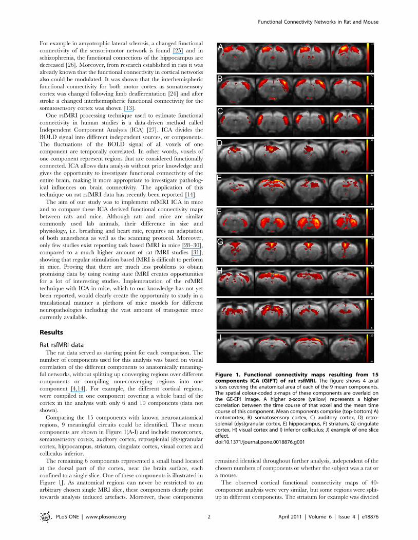
Comparing the 15 components with known neuroanatomical

regions, 9 meaningful circuits could be identified. These mean

components are shown in Figure 1(A-I) and include motorcortex,

somatosensory cortex, auditory cortex, retrosplenial (dys)granular

cortex, hippocampus, striatum, cingulate cortex, visual cortex and

colliculus inferior.

The remaining 6 components represented a small band located

at the dorsal part of the cortex, near the brain surface, each

confined to a single slice. One of these components is illustrated in

Figure 1J. As anatomical regions can never be restricted to an

arbitrary chosen single MRI slice, these components clearly point

towards analysis induced artefacts. Moreover, these components

remained identical throughout further analysis, independent of the

chosen numbers of components or whether the subject was a rat or

a mouse.

The observed cortical functional connectivity maps of 40-

component analysis were very similar, but some regions were split-

up in different components. The striatum for example was divided

Figure 1. Functional connectivity maps resulting from 15components ICA (GIFT) of rat rsfMRI. The figure shows 4 axialslices covering the anatomical area of each of the 9 mean components.The spatial colour-coded z-maps of these components are overlaid onthe GE-EPI image. A higher z-score (yellow) represents a highercorrelation between the time course of that voxel and the mean timecourse of this component. Mean components comprise (top-bottom) A)motorcortex, B) somatosensory cortex, C) auditory cortex, D) retro-splenial (dys)granular cortex, E) hippocampus, F) striatum, G) cingulatecortex, H) visual cortex and I) inferior colliculus; J) example of one sliceeffect.doi:10.1371/journal.pone.0018876.g001

Functional Connectivity Networks in Rat and Mouse

PLoS ONE | www.plosone.org 2 April 2011 | Volume 6 | Issue 4 | e18876

in two components, one representing the ventrolateral part, the

other representing the dorsomedial part of the striatum (shown in

Figure 2), indicating that within the striatum these two regions

could have slightly different LFF dynamics. Moreover, panel B in

the figure shows that there is some similarity in the dynamics of the

striatum and the somatosensory cortex. Also the colliculus inferior

and cingulated cortex were separated in the 40 as compared to the

15 component analysis and the piriform cortex came out as an

additional component.

Overall this resulted in an extension to 19 anatomically relevant

components. The 6 artefactual components, as stated before,

appeared very comparable in this analysis. Since the remaining

components were either more diffuse, or only comprising a few

voxels, it was impossible to co-localize these with the atlas.

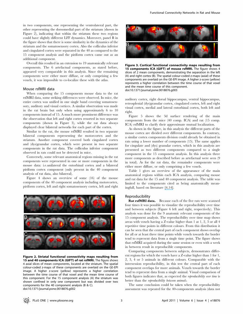
Mouse rsfMRI dataWhen comparing the 15 components mouse data to the rat

rsfMRI data, some striking differences were observed. In mice, the

entire cortex was unified in one single band covering somatosen-

sory, auditory and visual cortices. A similar observation was made

in the rat brain but only when using approximately 6 to 10

components instead of 15. A much more prominent difference was

the observation that left and right cortex resorted in two separate

components (shown in Figure 3), while the rat data always

displayed clear bilateral networks for each part of the cortex.

Similar to the rat, the mouse rsfMRI resulted in two separate

bilateral components representing the motorcortex and the

striatum. Another component covered both cingulated cortex

and (dys)granular cortex, which were present in two separate

components in the rat data. The colliculus inferior component

observed in rats could not be detected in mice.

Conversely, some relevant anatomical regions missing in the rat

components were represented in one or more components in the

mouse data: i.e.unilateral the entorhinal cortex and a bilateral

piriform cortex component (only present in the 40 component

analysis of rat data, also bilateral).

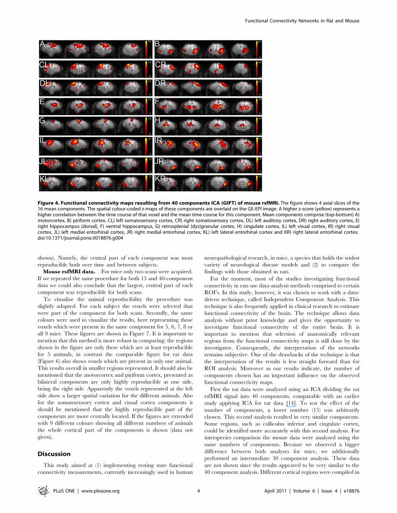
Figure 4 shows an overview of some (16) of the mouse

components of the 40 component analysis including motorcortex,

piriform cortex, left and right somatosensory cortex, left and right

auditory cortex, right dorsal hippocampus, ventral hippocampus,

retrosplenial (dys)granular cortex, cingulated cortex, left and right

visual cortex, medial and lateral entorhinal cortex, both left and

right.

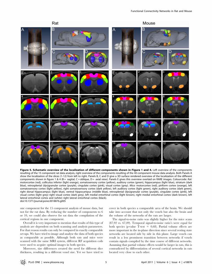
Figure 5 shows the 3d surface rendering of the main

components from the mice (40 comp. ICA) and rat (15 comp.

ICA) rsfMRI to clarify their approximate mutual localization.

As shown in the figure, in this analysis the different parts of the

mouse cortex are divided over different components. In contrary,

a similar cortex components division could already be obtained in

rats using a lower number of components (15). The same applies

for cingulate and (dys) granular cortex, which in this analysis are

presented as two different components compared to a single

component in the 15 component analysis. In this analysis three

more components as described before as artefactual were seen (9

in total). As for the rat data, the remainder components were

either more diffuse, or only comprising a few voxels.

Table 1 gives an overview of the appearance of the main

anatomical regions within each ICA analysis, comparing mouse

and rat data for the 15 and 40 component analysis. The table was

limited to the components cited as being anatomically mean-

ingfull, based on literature [4,14].

ReproducibilityRat rsfMRI data. Because each of the five rats were scanned

four times it was possible to visualize the reproducibility over time

and between subjects (Figure 6 left and right, respectively). This

analysis was done for the 9 anatomic relevant components of the

15 component analysis. The reproducibility over time map shows

areas with voxels having a Z-value higher than 1 at 1, 2, 3 or all 4

repetitive time points in different colours. From this distribution it

can be seen that the central part of each component shows overlap

for all or at least three time points while voxels towards the border

tend to represent data from a single time point. The figure shows

that rsfMRI acquired during the same session or even with a week

in between result in reproducible components.

Comparing components between subjects, demonstrates differ-

ent regions for which the voxels have a Z-value higher than 1 for 1,

2, 3, 4 or 5 animals in different colours. Comparable with the

intersession reproducibility, in this test the central part of each

component overlaps for more animals. Voxels towards the border

tend to represent data from a single animal. Visual comparison of

both figures indicates that, as expected the reproducibility over time is

better than the reproducibility between animals.

The same conclusion could be taken when the reproducibility

assessment was repeated for the 40-components analysis (data not

Figure 2. Striatal functional connectivity maps resulting from15 and 40 components ICA (GIFT) of rat rsfMRI. The figure shows4 axial slices of mean components, located at the striatum. The spatialcolour-coded z-maps of these components are overlaid on the GE-EPIimage. A higher z-score (yellow) represents a higher correlationbetween the time course of that voxel and the mean time course ofthis component. For the 15 component analysis (A) the striatum wasshown confined in only one component but was divided over twocomponents for the 40 component analysis (B & C).doi:10.1371/journal.pone.0018876.g002

Figure 3. Cortical functional connectivity maps resulting from15 components ICA (GIFT) of mouse rsfMRI. The figure shows 4slices of 2 mean components, demonstrating the separation in the left(A) and right cortex (B). The spatial colour-coded z-maps (axial) of thesecomponents are overlaid on the GE-EPI image. A higher z-score (yellow)represents a higher correlation between the time course of that voxeland the mean time course of this component.doi:10.1371/journal.pone.0018876.g003

Functional Connectivity Networks in Rat and Mouse

PLoS ONE | www.plosone.org 3 April 2011 | Volume 6 | Issue 4 | e18876

shown). Namely, the central part of each component was most

reproducible both over time and between subjects.

Mouse rsfMRI data. For mice only two scans were acquired.

If we repeated the same procedure for both 15 and 40-component

data we could also conclude that the largest, central part of each

component was reproducible for both scans.

To visualize the animal reproducibility the procedure was

slightly adapted. For each subject the voxels were selected that

were part of the component for both scans. Secondly, the same

colours were used to visualize the results, here representing those

voxels which were present in the same component for 5, 6, 7, 8 or

all 9 mice. These figures are shown in Figure 7. It is important to

mention that this method is more robust in comparing: the regions

shown in the figure are only these which are at least reproducible

for 5 animals, in contrast the comparable figure for rat data

(Figure 6) also shows voxels which are present in only one animal.

This results overall in smaller regions represented. It should also be

mentioned that the motorcortex and piriform cortex, presented as

bilateral components are only highly reproducible at one side,

being the right side. Apparently the voxels represented at the left

side show a larger spatial variation for the different animals. Also

for the somatosensory cortex and visual cortex components it

should be mentioned that the highly reproducible part of the

components are more centrally located. If the figures are extended

with 9 different colours showing all different numbers of animals

the whole cortical part of the components is shown (data not

given).

Discussion

This study aimed at (1) implementing resting state functional

connectivity measurements, currently increasingly used in human

neuropathological research, in mice, a species that holds the widest

variety of neurological disease models and (2) to compare the

findings with those obtained in rats.

For the moment, most of the studies investigating functional

connectivity in rats use data-analysis methods comprised to certain

ROI’s. In this study, however, it was chosen to work with a data-

driven technique, called Independent Component Analysis. This

technique is also frequently applied in clinical research to estimate

functional connectivity of the brain. The technique allows data

analysis without prior knowledge and gives the opportunity to

investigate functional connectivity of the entire brain. It is

important to mention that selection of anatomically relevant

regions from the functional connectivity maps is still done by the

investigator. Consequently, the interpretation of the networks

remains subjective. One of the drawbacks of the technique is that

the interpretation of the results is less straight forward than for

ROI analysis. Moreover as our results indicate, the number of

components chosen has an important influence on the observed

functional connectivity maps.

First the rat data were analyzed using an ICA dividing the rat

rsfMRI signal into 40 components, comparable with an earlier

study applying ICA for rat data [14]. To test the effect of the

number of components, a lower number (15) was arbitrarily

chosen. This second analysis resulted in very similar components.

Some regions, such as colliculus inferior and cingulate cortex,

could be identified more accurately with this second analysis. For

interspecies comparison the mouse data were analysed using the

same numbers of components. Because we observed a bigger

difference between both analyses for mice, we additionally

performed an intermediate 30 component analysis. These data

are not shown since the results appeared to be very similar to the

40 component analysis. Different cortical regions were compiled in

Figure 4. Functional connectivity maps resulting from 40 components ICA (GIFT) of mouse rsfMRI. The figure shows 4 axial slices of the16 mean components. The spatial colour-coded z-maps of these components are overlaid on the GE-EPI image. A higher z-score (yellow) represents ahigher correlation between the time course of that voxel and the mean time course for this component. Mean components comprise (top-bottom) A)motorcortex, B) piriform cortex, CL) left somatosensory cortex, CR) right somatosensory cortex, DL) left auditory cortex, DR) right auditory cortex, E)right hippocampus (dorsal), F) ventral hippocampus, G) retrosplenial (dys)granular cortex, H) cingulate cortex, IL) left visual cortex, IR) right visualcortex, JL) left medial entorhinal cortex, JR) right medial entorhinal cortex, KL) left lateral entorhinal cortex and KR) right lateral entorhinal cortex.doi:10.1371/journal.pone.0018876.g004

Functional Connectivity Networks in Rat and Mouse

PLoS ONE | www.plosone.org 4 April 2011 | Volume 6 | Issue 4 | e18876

one component for the 15 component analysis of mouse data, but

not for the rat data. By reducing the number of components to 6

or 10, we could also observe for rat data the compilation of the

cortical regions in one component.

Overall it is very important to mention that results of this type of

analysis are dependent on both scanning and analysis parameters.

For that reason results can only be compared in exactly comparable

set-ups. We have tried to image and analyse the data of both species

as comparable as possible. Although both rats and mice were

scanned with the same MRI system, different RF acquisition coils

were used to acquire optimal images in both species.

Moreover, size differences created the need for different slice

thickness, resulting in a different voxel size. Yet we have tried to

cover in both species a comparable area of the brain. We should

take into account that not only the voxels but also the brain and

the volume of the networks of the rats are larger.

The signal-to-noise ratio was slightly higher for the mice scans

(87,92 vs. 67,09). Temporal signal-to-noise ratio’s were equal for

both species (p-value T-test = 0,68). Partial volume effects are

more important in the in-plane direction since several resting state

networks are located side by side in this plane. Large voxels can

result in a less prominent transition between networks if voxels

contain signals compiled by the time course of different networks.

Assuming that partial volume effects would be larger in rats, this is

contradicted by differentiation of several cortical networks in rats

located very close to each other.

Figure 5. Schematic overview of the localization of different components shown in Figure 1 and 4. Left overview of the componentsresulting of the 15 component rat data analysis, right overview of the components resulting of the 40 component mouse data analysis. Both Panels Ashow the localization of the slices (1-12) from left to right. Panels B, C and D give a 3D surface rendered overview of the localization of the differentcomponents shown in figure 1 & 4 (B = sagital, C = oblique, D = axial view). Panels E gives this overview overlaid on RARE images. Colourcode: Rat:motorcortex (red), colliculus inferior (light orange), somatosensory cortex (yellow), auditory cortex (green), hippocampus (light blue), striatum (darkblue), retrosplenial (dys)granular cortex (purple), cingulate cortex (pink), visual cortex (grey). Mice: motorcortex (red), piriform cortex (orange), leftsomatosensory cortex (light yellow), right somatosensory cortex (dark yellow), left auditory cortex (light green), right auditory cortex (dark green),right dorsal hippocampus (light blue), ventral hippocampus (middle blue), retrosplenial (dys)granular cortex (purple), cingulate cortex (pink), leftvisual cortex (light grey) right visual cortex (dark grey), left medial entorhinal cortex (light brown), right medial entorhinal cortex (dark brown), leftlateral entorhinal cortex and (white) right lateral entorhinal cortex (black).doi:10.1371/journal.pone.0018876.g005

Functional Connectivity Networks in Rat and Mouse

PLoS ONE | www.plosone.org 5 April 2011 | Volume 6 | Issue 4 | e18876

Then in processing also a lot of parameters have to be taken into

account, that could influence the outcome of the analysis. First of

all, the smoothing kernel - which had a size of approximately 2

voxels [13,32] - was slightly adapted for the mouse data but due to

a rectangular matrix and square FOV this was not completely

comparable for both species. Repeating the analysis with

smoothing kernels exactly two-by-two voxels for both species

resulted in components comparable to those presented in the

paper. Also results with and without temporal filtering were

compared. This was done using a band pass filter (0.01–0.1 Hz).

In human research the limit of 0.1 Hz is used to exclude high

frequency physiological fluctuations. It should be mentioned that

due to the high cardiac and breathing rates in rodents the 0.1 Hz

filter is insufficient [21] although it does not compromise the

presented analysis strategy, because ICA can identify/isolate

undersampled (aliased) processes.

We have chosen to apply this filter, in convergence with the

ICA study of Hutchison et al. to compare the results. The results

without filter were very comparable although more artefactual

components were present in the non-filtered analyses, and some

regions e.g. the hippocampus component could not be discerned.

We also repeated the analyses with and without applying a spatial

brain mask to the data. The effect of this mask was minimal,

resulting in almost identical components. Furthermore ICA can be

performed using different algorithms [33] and different numbers

of components which has an important influence on the results, as

proven in this paper.

Table 1. Overview of the appearance of the main anatomical regions within each ICA analysis, comparing mouse and rat data forthe 15 and 40 component analysis.

Rat Mouse

15 40 15 40

motorcortex 1 component 1 component 1 component 1 component

Somatosensory cortex (SSC) 1 component 1 component 2 unilateral components (left + right)covering SSC, AC and VC

2 components (left + right)

auditory cortex (AC) 1 component 1 component 2 unilateral components (left + right)covering SSC, AC and VC

2 components (left + right)

Retrosplenial (dys)granularcortex (RC)

1 component 1 component 1 component covering RC and CC 1 component

hippocampus 1 component 1 component 1 component 2 components (dorsal + ventral)

striatum 1 component 2 components / /

cingulate cortex (CC) 1 component 3 components 1 component covering RC and CC 1 component

visual cortex 1 component 2 components 2 unilateral components covering SSC,AC and VC

2 components (left + right)

inferior colliculus 1 component 6 components / /

piriform cortex / 1 component 1 component 1component

entorhinal cortex / / entorhinal cortex 1 component (right) 4 component left medial andlateral + Right medial andlateral)

doi:10.1371/journal.pone.0018876.t001

Figure 6. Reproducibility between sessions and betweensubjects of 15 components ICA (GIFT) of rat rsfMRI. Left: Picturesshowing session cumulative score maps for 9 selected mean ICA ratcomponents (central slice) over the different time points overlaid on theGE-EPI image. Colour-code: voxels with z-value higher than 1 for onetime point (blue), two time points (blue-green), three time points(orange), four time points (red). Right: Pictures showing animalcumulative score maps for 9 selected ICA rat components (centralslice) of the five rats overlaid on the GE-EPI image. Colour-code: voxelswith z-value higher than 1 for one animal (blue), two animals (blue-green), three animals (orange), four animals (red), five animals (pink).doi:10.1371/journal.pone.0018876.g006

Figure 7. Reproducibility between subjects of 40 componentsICA (GIFT) of mouse rsfMRI. Pictures showing animal cumulativescore maps for 16 selected ICA mice components (central slice) of thenine mice overlaid on the GE-EPI image. Colour-code: voxels with z-value higher than 1 for five animals (blue), six animals (blue-green),seven animals (orange), eight animals (red), nine animals (pink).doi:10.1371/journal.pone.0018876.g007

Functional Connectivity Networks in Rat and Mouse

PLoS ONE | www.plosone.org 6 April 2011 | Volume 6 | Issue 4 | e18876

An important difference between human MRI and small animal

imaging is the need for anaesthesia to avoid movement. This is an

important issue since both the BOLD response as well as the

temporal correlation of LFFs between regions can be affected by

anaesthesia [34]. We selected medetomidine of which it has been

proven that it preserves functional connectivity [22] above all

other options such as a-chloralose, isoflurane or ketamine/

xylazine because of their toxicity, known deteriorating effect on

functional connectivity or absence of information on the effect on

resting state, respectively [35].

Interestingly, a clinical study reported recently that resting state

data obtained under anaesthesia can have a significant diminishing

effect on the fronto-parietal networks while functional connectivity

at the early sensory cortices was relatively preserved. Related hereto

in anaesthetised animals these sensory networks can be observed

whereas the fronto-parietal networks (default mode network and

executive control network), related to higher functions, remained

undetected. This indicates that even if such networks are present in

rodents they would hardly be assessable under anaesthesia [36].

In our study we discerned separate sensorimotor, visual and

auditory networks comparable to what has been described in

humans [4,37]. The cingulate cortex, represented in both rodent

species as a single component, is separated into a posterior and an

anterior part in humans and belongs to the default mode network

[4]. This human network also includes the medial prefrontal

cortex (see Figure 1, component G).

The other regions within the human network (bilaterally the

medial and lateral temporal lobe, the retrosplenial and lateral

temporal cortex, precuneus and hippocampal formation [38])

could however not be resolved in rodents.

While in humans primary and secondary visual cortical areas are

separated in two components [4,37] both are restricted to one

component in the rodent brain. This could be related to the

important anatomical difference in the visual system resulting from

the frontal versus lateral sight in humans versus rodents respectively.

Moreover, in our rat study the visual cortex component was smaller

as compared to the findings by Hutchison [14] and our mouse data.

This difference could be explained by the reported visual cortex

deficits [39] in albino rats like the Sprague-Dawley rats we used

compared to the non albino Long Evans strain used by Hutchison

and coworkers and the non albino (C57BL/6) mice we used.

Some regions, typically found in rodents, but not mentioned as

being part of a resting state network in human research, e.g. the

inferior colliculus, the entorhinal and the piriform cortex, were

also found each in a separate left and right component. In rats, the

entorhinal cortex comprises 4 regions (dorsolateral, dorsointer-

mediate, ventral intermediate and medial) while in mice it only

comprises a medial and lateral region which could be displayed in

different components [40]. Because of this higher fragmentation of

the rat brain structures it is possible that in rats all different parts

have a slightly different temporal profile. This could explain why

those parts of the cortex could be recognized for mice, but not for

rats. The piriform cortex, while not discriminated in human

studies, emerges in both rats and mice upon 40 component ICA

analysis and probably reflects the more important role of olfaction

in rodents as compared to humans.

Moreover, we described the existence of a component showing

striatocortical connectivity which can be interesting for example in

animal models for Parkinson’s [41] and Huntington’s disease [42]

as in this pathology the projections between the aforementioned

areas are affected and are a target for therapeutic strategies.

Most of the observed components were in agreement with

another recent study using ICA rsfMRI on the rat brain [14]

although some differences should be mentioned in the experimental

setup: the use of anaesthesia (medetomidine vs. xylazine-ketamine

and isoflurane), the slice direction (axial vs coronal) and the strain of

rats (Sprague-Dawley vs. Long Evans). Different to our findings,

most of their components showed a degree of laterality which might

be due to the difference in applied anaesthesia as medetomidine

better preserves functional connections [14].

The detection of unilateral components in mice compared to

bilateral components for the same networks in rats indicate that

the LFF of left and right cortices are different in mice while being

similar in rats. This could possibly reflect a lower interhemispheric

functional connectivity in mice. Since the same homotopic

interhemispheric cortical connections are found in both rats and

mice [37] there is probably no anatomical substance for this

difference. It is known that functionally linked resting-state

networks reflect the underlying structural connectivity, since most

of the nodes of a single resting state network are interconnected

with white matter tracts [43]. The same is true for these cortical

regions, connected through the corpus callosum in both species.

Consequently the difference is located on a functional level

rather than the underlying anatomical structure, indicating the

need to study the temporal characteristics of the low frequency

BOLD signal in the anaesthetized mouse brain and compare this

with earlier findings of rats [10].

Moreover it would be interesting to study the differences

between both species using a electrophysiological read-out. It is

known that there is a strong correlation in LFFs measured with

BOLD fMRI and fluctuations discerned in the power of the local

field potential (LFP) signal as measured at different parts of the

cortex in monkeys [16,44]. Studying these LFPs in both rats and

mice could give more insight in what was found here. Although we

should mention that it is impossible to validate the results with the

same study set-up since electrophysiological recordings can’t be

performed under medetomidine anesthesia.

Using different numbers of independent components revealed the

need for higher number of components in order to discriminate

different parts of the cortex in mice as compared to rats. This could

reflect a more subtle difference in LFF between different neuronal

networks in mice or might be linked to their smaller brain volume.

To gain more insight in what causes these differences there is a

need to perform a parallel electrophysiological study in the future.

Similarly, it could be anticipated that a differential use of the

number of components might lead to detection of abnormalities in

models linked to disease induced LFF differences between

networks that might otherwise remain uncovered.

Materials and Methods

Ethics statementAll procedures were performed in accordance with the

European guidelines for the care and use of laboratory animals

(86/609/EEC) and were approved by the Committee on Animal

Care and Use at the University of Antwerp, Belgium.

AnimalsFive male Sprague-Dawley rats (Charles River Laboratories,

Wilmington, USA) (Body weight 454660 g) of approximately 12

weeks and 9 male C57BL/6 mice (Charles River Laboratories,

Wilmington, USA) (body weight 2562 g) of approximately 13

weeks were imaged. Rats were imaged at 2 time points, with one

week in between, and at each time point two consecutive resting

state scans were acquired. Mice were imaged at one time point, at

which two consecutive resting state scans were acquired.

Taking into account the age of sexual maturity and neuronal

development of both species we can assume that the developmental

age at the time of scanning is comparable for rats and mice [45–47].

Functional Connectivity Networks in Rat and Mouse

PLoS ONE | www.plosone.org 7 April 2011 | Volume 6 | Issue 4 | e18876

rsfMRI procedureRats. A rectal thermistore was inserted to monitor the body

temperature and keep it at (37.060.5)uC by means of a feedback-

controlled warm air circuitry (MR-compatible Small Animal

Heating System, SA Instruments, Inc.).

Breathing rate, heart rate and blood oxygen saturation were

monitored using a pulse oximeter positioned at the hind limb and

a pressure sensitive sensor under the rat (MR-compatible Small

Animal Monitoring and Gating System, SA Instruments, Inc).

During handling (weighing and immobilization) rats were

anaesthetized with isoflurane (2% IsoFlo, Abott, Illinois, USA)

administered in a mixture of 30% O2 and 70% N2. During the

resting state experiment, animals were sedated using medetomi-

dine (Domitor, Pfizer, Karlsruhe, Germany). First a bolus of

0.05 mg/kg was injected subcutaneously and isoflurane was

discontinued after 5 minutes.

A continuous infusion of medetomidine (0.1 mg/kg/h) was

started 15 minutes after bolus injection [48]. After the scanning

procedure, medetomidine was antagonized by an injection of

atipamezole (0.1 mg/kg) (Antisedan, Pfizer, Karlsruhe, Germany).

Imaging was done on a 9.4T Biospec scanner (Bruker,

Ettlingen, Germany). Images were acquired with a Bruker linear

transmit volume coil and a parallel receive surface array designed

for rat head MRI. First three orthogonal Turbo RARE T2-

weighted images were acquired to uniform the slice positioning

(TR 2500 ms, effective TE 33 ms, 15 slices, 1 mm). Then the

resting state data-sets were acquired using single shot gradient

echo EPI (Echo Planar Imaging) with TR 2000 ms and TE 16 ms.

Twelve axial slices of 1 mm and a gap of 0.1 mm were recorded

with a FOV of (30630) mm2 and matrix size of 1286128 resulting

in voxel dimensions of (0.2360.2361) mm3. The used bandwidth

was 400 kHz (3125 Hz/voxel). Each of the rsfMRI data

comprised 150 repetitions, resulting in a scanning time of 5

minutes for each rsfMRI dataset.Mice. The same monitoring procedures were followed during

the mice scans and the same principle was used to sedate the mice.

A bolus of 0.3 mg/kg medetomidine was followed by continuous

infusion of 0.6 mg/kg/h [30].

Imaging was also done on a 9.4T Biospec scanner (Bruker,

Ettlingen, Germany). Images were acquired with a standard

Bruker crosscoil set-up using a quadrature volume coil and a

quadrature surface coil for mice. First three orthogonal Turbo

RARE T2-weighted images were acquired to uniform the slice

positioning (TR 2500 ms, effective TE 33 ms, 9 slices, 0.5 mm).

Then the resting state data-sets were acquired using single shot

gradient echo EPI with TR 2000 ms and TE 15 ms. Twelve axial

slices of 0.4 mm and a gap of 0.1 mm were recorded with a FOV

of (20620) mm2 and matrix size of 128664 resulting in voxel

dimensions of (0.1660.3160.4) mm3. The used bandwidth was

400 kHz (3125 Hz/voxel in read/6250 Hz/voxel in phase

encoding). Hundred fifty repetitions were taken, resulting in a 5

minute scanning time for each rsfMRI dataset.

PreprocessingPreprocessing was done in SPM8 (http://www.fil.ion.ucl.ac.uk/

spm/software/spm8/). A common protocol for preprocessing of

fMRI data was followed. First, all images within each session were

realigned to the first image. This was done using a least squares

approach and a 6 parameter (rigid body) spatial transformation.

Second, all datasets were normalized. The first step of the

normalisation is a global 12-parameter affine transformation based

on the maximalization of the product of the likelihood function

(derived from the residual squared difference) and the prior

function (which is based on the probability of obtaining a

particular set of zooms and shears) [49]. The affine registration

is followed by estimating nonlinear deformations, whereby the

deformations are defined by a linear combination of three

dimensional discrete cosine transform (DCT) basis functions

[50]. The matching involved simultaneously minimising the

membrane energies of the deformation fields and the residual

squared difference between the images and template (which is here

the rsfMRI images of the first animal). Finally, in plane smoothing

was done using a Gaussian kernel with Full width at half

maximum of (0.460.4) mm2 for the rat images and (0.360.4) mm2

for the mice images. A band pass filter (0.01 Hz–0.1 Hz) was

applied to the temporal data to rule out low frequency noise.

ProcessingTo estimate functional connectivity, ICA was performed, using

GIFT (Group ICA of fMRI toolbox: http://icatb.sourceforge.net/),

working in Matlab2008 (www.mathworks.com), and implementing

spatial ICA, indicating that the sources are estimated as being

statistically spatially independent. The GIFT toolbox is especially

designed to analyze group rsfMRI data, and works in three steps.

First, a data reduction is done, by principal component analysis.

This was done in two steps where first the functional data were

reduced, followed by concatenation of the data in groups. Second,

a group ICA is performed using the Infomax algorithm. Last, a

back reconstruction of the data to single subject independent

components and time courses was done.

To investigate the effect of the number of components, ICA of

rat rsfMRI data was repeated several times with different preset

component numbers.

The analysis was repeated, setting the number at 6, 10, 15 and

40 components. The ICA on the rsfMRI data of mice was assessed

with a preset of 15, 30 and 40 components.

Author Contributions

Conceived and designed the experiments: EJ MV AVdL. Performed the

experiments: EJ JVA. Analyzed the data: EJ GDV. Contributed reagents/

materials/analysis tools: EJ JVA. Wrote the paper: EJ. Revised the article:

JVA GDV AVdL MV.

References

1. Biswal B, Yetkin FZ, Haughton VM, Hyde JS (1995) Functional connectivity inthe motor cortex of resting human brain using echo-planar MRI. Magn Reson

Med 34: 537–541.

2. van den Heuvel MP, Hulshoff Pol HE (2010) Exploring the brain network: areview on resting-state fMRI functional connectivity. Eur Neuropsychopharma-

col 20: 519–534.

3. Damoiseaux JS, Beckmann CF, Arigita EJ, Barkhof F, Scheltens P, et al. (2008)

Reduced resting-state brain activity in the ‘‘default network’’ in normal aging.Cereb Cortex 18: 1856–1864.

4. Damoiseaux JS, Rombouts SA, Barkhof F, Scheltens P, Stam CJ, et al. (2006)

Consistent resting-state networks across healthy subjects. Proc Natl Acad

Sci U S A 103: 13848–13853.

5. Greicius MD, Flores BH, Menon V, Glover GH, Solvason HB, et al. (2007) Resting-state functional connectivity in major depression: abnormally increased contributions

from subgenual cingulate cortex and thalamus. Biol Psychiatry 62: 429–437.

6. Rombouts SA, Damoiseaux JS, Goekoop R, Barkhof F, Scheltens P, et al. (2009)Model-free group analysis shows altered BOLD FMRI networks in dementia.

Hum Brain Mapp 30: 256–266.

7. Bluhm RL, Miller J, Lanius RA, Osuch EA, Boksman K, et al. (2007)

Spontaneous low-frequency fluctuations in the BOLD signal in schizophrenicpatients: anomalies in the default network. Schizophr Bull 33: 1004–1012.

8. Wise RG, Ide K, Poulin MJ, Tracey I (2004) Resting fluctuations in arterial

carbon dioxide induce significant low frequency variations in BOLD signal.

Neuroimage 21: 1652–1664.

Functional Connectivity Networks in Rat and Mouse

PLoS ONE | www.plosone.org 8 April 2011 | Volume 6 | Issue 4 | e18876

9. Gusnard DA, Raichle ME, Raichle ME (2001) Searching for a baseline:

functional imaging and the resting human brain. Nat Rev Neurosci 2: 685–694.

10. Kannurpatti SS, Biswal BB, Kim YR, Rosen BR (2008) Spatio-temporal

characteristics of low-frequency BOLD signal fluctuations in isoflurane-

anesthetized rat brain. Neuroimage 40: 1738–1747.

11. Zhao F, Zhao T, Zhou L, Wu Q, Hu X (2008) BOLD study of stimulation-

induced neural activity and resting-state connectivity in medetomidine-sedated

rat. Neuroimage 39: 248–260.

12. Biswal BB, Kannurpatti SS (2009) Resting-state functional connectivity in

animal models: modulations by exsanguination. Methods Mol Biol 489:

255–274.

13. van Meer MP, van der Marel K, Otte WM, Berkelbach van der Sprenkel JW,

et al. (2010) Correspondence between altered functional and structural

connectivity in the contralesional sensorimotor cortex after unilateral stroke in

rats: a combined resting-state functional MRI and manganese-enhanced MRI

study. J Cereb Blood Flow Metab 30: 1707–1711.

14. Hutchison RM, Mirsattari SM, Jones CK, Gati JS, Leung LS (2010) Functional

networks in the anesthetized rat brain revealed by independent component

analysis of resting-state FMRI. J Neurophysiol 103: 3398–3406.

15. Vincent JL, Patel GH, Fox MD, Snyder AZ, Baker JT, et al. (2007) Intrinsic

functional architecture in the anaesthetized monkey brain. Nature 447: 83–86.

16. Shmuel A, Leopold DA (2008) Neuronal correlates of spontaneous fluctuations

in fMRI signals in monkey visual cortex: Implications for functional connectivity

at rest. Hum Brain Mapp 29: 751–761.

17. Moeller S, Nallasamy N, Tsao DY, Freiwald WA (2009) Functional connectivity

of the macaque brain across stimulus and arousal states. J Neurosci 29:

5897–5909.

18. Teichert T, Grinband J, Hirsch J, Ferrera VP (2010) Effects of heartbeat and

respiration on macaque fMRI: implications for functional connectivity.

Neuropsychologia 48: 1886–1894.

19. Bifone A, Gozzi A, Schwarz AJ (2010) Functional connectivity in the rat brain: a

complex network approach. Magn Reson Imaging 28: 1200–1209.

20. Magnuson M, Majeed W, Keilholz SD (2010) Functional connectivity in blood

oxygenation level-dependent and cerebral blood volume-weighted resting state

functional magnetic resonance imaging in the rat brain. J Magn Reson Imaging

32: 584–592.

21. Kalthoff D, Seehafer JU, Po C, Wiedermann D, Hoehn M (2010) Functional

connectivity in the rat at 11.7T: Impact of physiological noise in resting state

fMRI. Neuroimage Epub ahead of print.

22. Pawela CP, Biswal BB, Hudetz AG, Schulte ML, Li R, et al. (2009) A protocol

for use of medetomidine anesthesia in rats for extended studies using task-

induced BOLD contrast and resting-state functional connectivity. Neuroimage

46: 1137–1147.

23. Pawela CP, Biswal BB, Cho YR, Kao DS, Li R, et al. (2008) Resting-state

functional connectivity of the rat brain. Magn Reson Med 59: 1021–1029.

24. Pawela CP, Biswal BB, Hudetz AG, Li R, Jones SR, et al. (2010)

Interhemispheric neuroplasticity following limb deafferentation detected by

resting-state functional connectivity magnetic resonance imaging (fcMRI) and

functional magnetic resonance imaging (fMRI). Neuroimage 49: 2467–2478.

25. Mohammadi B, Kollewe K, Samii A, Krampfl K, Dengler R, et al. (2009)

Decreased brain activation to tongue movements in amyotrophic lateral sclerosis

with bulbar involvement but not Kennedy syndrome. J Neurol 256: 1263–1269.

26. Zhou Y, Shu N, Liu Y, Song M, Hao Y, et al. (2008) Altered resting-state

functional connectivity and anatomical connectivity of hippocampus in

schizophrenia. Schizophr Res 100: 120–132.

27. van de Ven V, Formisano E, Prvulovic D, Roeder CH, Linden DE (2004)

Functional connectivity as revealed by spatial independent component analysisof fMRI measurements during rest. Hum Brain Mapp 22: 165–178.

28. Ahrens ET, Dubowitz DJ (2001) Peripheral somatosensory fMRI in mouse at

11.7 T. NMR Biomed 14: 318–324.29. Nair G, Duong TQ (2004) Echo-planar BOLD fMRI of mice on a narrow-bore

9.4 T magnet. Magn Reson Med 52: 430–434.30. Adamczak JM, Farr TD, Seehafer JU, Kalthoff D, Hoehn M (2010) High field

BOLD response to forepaw stimulation in the mouse. Neuroimage 51: 704–712.

31. Van Der Linden A, van Camp N, Ramos-Cabrer P, Hoehn M (2007) Currentstatus of functional MRI on small animals: application to physiology,

pathophysiology, and cognition. NMR Biomed 20: 522–545.32. Majeed W, Magnuson M, Keilholz SD (2009) Spatiotemporal dynamics of low

frequency fluctuations in BOLD fMRI of the rat. J Magn Reson Imaging 30:384–393.

33. Hyvarinen A, Oja E (2000) Independent component analysis: algorithms and

applications. Neural Netw 13: 411–430.34. Williams KA, Magnuson M, Majeed W, Laconte SM, Peltier SJ, et al. (2010)

Comparison of alpha-chloralose, medetomidine and isoflurane anesthesia forfunctional connectivity mapping in the rat. Magn Reson Imaging 28: 995–1003.

35. Silverman J, Muir WW, III (1993) A review of laboratory animal anesthesia with

chloral hydrate and chloralose. Lab Anim Sci 43: 210–216.36. Boveroux P, Vanhaudenhuyse A, Bruno MA, Noirhomme Q, Lauwick S, et al.

(2010) Breakdown of within- and between-network Resting State FunctionalMagnetic Resonance Imaging Connectivity during Propofol-induced Loss of

Consciousness. Anesthesiology 113: 1038–1053.37. Beckmann CF, DeLuca M, Devlin JT, Smith SM (2005) Investigations into

resting-state connectivity using independent component analysis. Philos

Trans R Soc Lond B Biol Sci 360: 1001–1013.38. Raichle ME, Snyder AZ (2007) A default mode of brain function: a brief history

of an evolving idea. Neuroimage 37: 1083–1090.39. Diykov DG (2005) Visual Cortex Defects in Albinos. The Internet Journal of

Ophthalmology and Visual Science 3.

40. Paxinos G, Watson C (1982) The Rat Brain in Stereotaxic Coordinates .41. Braak H, Sastre M, Del TK (2007) Development of alpha-synuclein

immunoreactive astrocytes in the forebrain parallels stages of intraneuronalpathology in sporadic Parkinson’s disease. Acta Neuropathol 114: 231–241.

42. Walker FO (2007) Huntington’s Disease. Semin Neurol 27: 143–150.43. van den Heuvel MP, Mandl RC, Kahn RS, Hulshoff Pol HE (2009)

Functionally linked resting-state networks reflect the underlying structural

connectivity architecture of the human brain. Hum Brain Mapp 30: 3127–3141.44. Scholvinck ML, Maier A, Ye FQ, Duyn JH, Leopold DA (2010) Neural basis of

global resting-state fMRI activity. Proc Natl Acad Sci U S A 107: 10238–10243.45. Adams N, Boice R (1983) A longitudinal study of dominance in an outdoor

colony of domestic rats. J Comp Psych 97: 24–31.

46. Fox JG, Barthold SW, Davisson MT, Newcomer CE, Quimby FW, et al. (2007)The mouse in Biomedical Research. Elsevier.

47. Clancy B, Finlay BL, Darlington RB, Anand KJ (2007) Extrapolating braindevelopment from experimental species to humans. Neurotoxicology 28:

931–937.48. Weber R, Ramos-Cabrer P, Wiedermann D, van Camp N, Hoehn M (2006) A

fully noninvasive and robust experimental protocol for longitudinal fMRI studies

in the rat. Neuroimage 29: 1303–1310.49. Ashburner J, Neelin P, Collins DL, Evans A, Friston K (1997) Incorporating

prior knowledge into image registration. Neuroimage 6: 344–352.50. Buchel C, Wise RJ, Mummery CJ, Poline JB, Friston KJ (1996) Nonlinear

regression in parametric activation studies. Neuroimage 4: 60–66.

Functional Connectivity Networks in Rat and Mouse

PLoS ONE | www.plosone.org 9 April 2011 | Volume 6 | Issue 4 | e18876