DIPARTIMENTO DI MATEMATICA“Francesco Brioschi”

POLITECNICO DI MILANO

A Mathematical Proposal to Evaluate

Functional Connectivity Strongness in

Complex Brain Networks

Finotelli, P.; Dulio, P.

Collezione dei Quaderni di Dipartimento, numero QDD 187

Inserito negli Archivi Digitali di Dipartimento in data 15-10-2014

Piazza Leonardo da Vinci, 32 - 20133 Milano (Italy)

A Mathematical Proposal to Evaluate Functional

Connectivity Strongness in Complex Brain Networks

Paolo Finotellia, Paolo Dulioa

aPolitecnico di Milano, Dipartimento di Matematica “F.Brioschi”, Via Bonardi 9, 20133Milan, Italy

Abstract

The brain is a really complex organization of connectivity whose principalelements are neurons, synapses and brain regions. To date this connectiv-ity is not fully understood. Graph Theory represents a powerful tool in thestudy of brain networks.Though the complex organization of connectivity in human and animal brainhas found a great impulse by the use of Graph Theory, some points resultto be not very clear and need to be clarified, the weakness lies in the mis-matching between the mathematical and neuroscientific approach. In thispaper we focus, in particular, on two points: the concept of distance and amathematical approach in treating functional and structural connectivity bymeans of the introduction of the parameter time.It is known that neural connectivity is classify into three categories: struc-tural (or anatomical) connectivity, functional connectivity and effective con-nectivity. Structural connectivity can be visualized as the anatomical neuralnetwork in particular range of the life of human beings (and animals). Itrepresents the synaptic connections, or directed anatomical pathways derivedfrom neural tract tracing. It can be retained static only in absence of injuriesor cerebral illnesses, or far from the childhood and old age. The functionalconnectivity, i.e. the temporal correlations between remote neurophysiologi-cal events as reaction to well specific external stimuli (e.g. social paradigms,social cognitive functions or other specific tasks), interests cerebral areas notnecessarily close each other (in the sense of Euclidean distance). Aside weemphasize that the functional connectivity is very distinctive from effectiveconnectivity, i.e. the influence a neural system exerts over another one [27].The point is that these categories demand different kinds of graphs, exceptthe case of resting state. In this paper we formalize in a mathematical way

Preprint submitted to Reports of Math Department, QDD 187. December 16, 2014

the concept of distance and we introduce a function W (i, j, t) whose pecu-liarity is to give the weight of the edges composing the graph representingthe functional connectivity.This function W (i, j, t) depends on the position of nodes i, j and on thetime t at which a specific task is submitted to an health volunteer (and inin relation to the future to subjects affected by neurological diseases). In-terestingly this function, in particular cases, comes down to the probabilityof edge formation. Basically these particular cases are the resting state andwhen a particular task do not affect the cerebral region the nodes belong to.This second case is rare since when performing a task the region of interest,ROI, are well known.

Keywords: Brain networks, connectivity, distance, Graph Theory, time,edge weights

1. Introduction

The brain is a very complex structure, more precisely it has a compli-cated structural and functional connectivity between its basic constituents,i.e. neurons, synapses and brain regions.It is remarkable how substantially different systems share key characteristicsidentified by specific parameters such as: connectivity, centrality, clustering,hub, module (just to mention a few).If we restrict our attention to the brain connectivity, we should introduceother very important concepts in Neuromathematics:The connectome, defined as the network map of the anatomical connectionsin the brain (regardless it is human or animal).The parcellation which is the subdivision of the brain into areas or regions.The structural connectivity, that may be viewed as the anatomical descrip-tion of all connections between the different areas or neurons; when we talkabout projections we mean both the anatomical projections and directedanatomical pathways and synaptic connections between different neurons.The functional connectivity, which is strictly related with the activation ofdifferent cerebral areas not necessarily close to one another. It is the statis-tical dependence between the time series of two network nodes (e.g. brainregions or neurons) [68]. Importantly, there is a particular cerebral statewhere the functional and structural networks seems to coincide: the restingstate. The resting state network is the set of brain regions showing coherent

2

functional connectivity during task free spontaneous activity.As concerns the brain architecture, we cite the small world organization. Thesmall world organization is a network that has well defined characteristics:high level of clustering, or better, higher than that proper of regular networks,and an average shortest path length equal to the one observed in random net-works. Basically the small world organization shares characteristics typicalof both regular network and random network. It is important to clarify apoint regarding the small world organization: the length of a path. Abovewe have mentioned the “average shortest length path”, but concerning thelongest paths, we tacitly assume a small number of long-distance shortcutsamong locally connected nodes. A first approach states that these shortcutsare randomly placed within the network’s architecture but there are otherconjectures, in hub modeling, that suggest that these shortcuts aggregatehub nodes [67].We organize the paper as follows: section 2 has the purpose to show howconcepts proper of Graph Theory could be applied to shed more light onunaddressed questions in Neuroscience. In section 3 the definitions of Eu-clidean distance and of Discrete distance are shown, the goal is to emphasizethat these two distances cannot be employed together in the same analy-sis. In section 4 we propose a function whose scope is to assign a weightto an edge between two arbitrary nodes. Its most interesting characteristicsis the time-dependence. Finally, Section 5 is devoted to the discussion ofconclusions.

2. Graph Theory applied to Neuroscience: basics

In this section we are going to give some useful notions proper of GraphTheory and largely employed in Neuroscience: edge, node, graph, pathlength, efficiency, cost, hub, modularity, small world.

2.1. Edge, node, graph

A graph is a mathematical tool useful to describe a network. It is definedas a collection of nodes (also known as vertices) and of connection betweenedges, called edges.

2.2. Path length, mean path length, efficiency

Given two nodes i and j, the path length, li,j, is defined as the numberof edges that must be traversed in a sequence of connections starting from i

3

and arriving to j.The shortest path length is the minimum number of edges needed to linkone node to another. If we consider the whole-brain network architecture,than it is useful to define another topological concept: the mean shortestpath length, l (generally the reference scalar), is defined as the average ofthe shortest path lengths between any pair of nodes in the network. It mea-sures the distance (i.e., the number of edges) between any pair of nodes in anetwork or the extent of overall communication efficiency of a network. Themean path length can be short, for example in the case of random and/orcomplex networks, or long in the matter of regular lattices1. The mean pathlength is a measure of the global connectivity of the network and it is strictlyrelated to the global efficiency, its inverse. This means that random andcomplex networks have high global efficiency of parallel information transfer.On the contrary, for regular lattices, the global efficiency is low.Nonetheless the beauty of the intuitive definition of mean path length, thereis an important problem to face with: what about if the network has nodalpairs that have no connecting path? It is clear that the shortest path lengthfor such disconnected node pairs is infinite. It is possible to bypass this prob-lem by mean of the “harmonic mean”, that is calculating the reciprocal ofthe average of the reciprocals [42].A shorter distance means higher routing efficiency, because information isexchanged via fewer steps.

2.3. Cost

In this paper we shall not deal with the concept of cost of a graph. Forthe moment it is enough to know that the simplest estimator of the phys-ical cost of a network is the connection density, which is the proportion ofthe number of edges in the observed graph with respect to the number ofedges of the complete graph on the same number of vertices. The cost isthreshold-dependent [1], [38], the threshold plays a fundamental role in de-termining the adjacency matrix which resumes the vertex-adjacencies in thegiven graph. Thus, it is possible to represent various measures of networkorganization within each group as a function of the cost and to compare

1A regular lattice is a graph where each node has the same degree, i.e. each vertex hasthe same number of neighbors.

4

topological and anatomical properties of the graphs between groups underthe constraint that the number of edges is the same for each group over therange of the considered thresholds [15].

2.4. Hub, clustering

Clustering is the tendency of a small groups of nodes to form connectedtriangles (which are particular motifs2) or in other words the clustering coef-ficient (the measure of clustering) is an index of local structure, and has beeninterpreted as a measure of resilience to random error (if vertex i is lost, doits neighbors remain still connected?). Moreover clustering is related to thelocal efficiency, i.e. can be regarded as a measure of information transfer inthe immediate neighborhood of each node. It follows that clustering is a mea-sure of the local connectivity of a regional node. The clustering coefficient isdefined by the following ratio:

C =1

NGi(NGi

− 1)

∑j,k∈Gi

1

lj,k, (1)

Where Gi is the subgraph connected to the node i and lj,k is the (shortest)path length connecting the nodes j and k in the subgraph Gi.The clustering coefficient can be averaged across an entire network.

The basic question underpinning the concept of clustering is to determinethe likelihood of a vertex to have a degree k, i.e. the bayesian distributionP (V,E|k). Its advantage is that it is a global measure of a graph. Whilefor a random graph the corresponding degree distribution is a Gaussian one,many complex networks show non-Gaussian degree distributions. When agiven vertex shows a high-degree centrality, it is called hub [54].

2A motif is a small subset of network nodes and edges, forming a subgraph. Basicallymotifs are visually represented by building blocks (in analogy to driving elements thatare elaborated in a musical theme or composition) of different forms, and they are verycommon in contexts such as Genetics, Neuroscience, and other biological and artificialnetworks. Motifs occur in distinct classes, that can be distinguished according to the sizeof the motif, equal to the number of nodes (vertices), and the number and pattern ofinterconnections. For a more formal definition of motifs and related concepts we refer thereader to [53]

5

The hub is a node that occupies a central position inside the network. Acentral hub can be a connector hub, i.e. an hub that is mainly connected tovertices in other modules, or a provincial hub, which is a high-degree nodethat is primarily connected to node in the same module. Provincial andconnector hubs may play different functional roles within a network. It isinteresting to note that a connector hub mediate a high proportion of inter-modular, and often long-distance, connections.

There are several criteria/measures of a graph to identify centrality, butnone of them is unquestionable to select an hub. A few of them are describedbelow:

2.5. Node degree

Node degree is the number of edge attached to a single node. Highlyconnected nodes have large node degree. The node degree distribution rep-resents the probability of a given node degree over all node degrees in thenetwork.

2.6. Closeness centrality

Closeness is based on the length of the average shortest path between anode and all nodes in the graph. It can be identified as the inverse of thesum of all length paths joining two arbitrary nodes:

Cc(i) =1∑n

j=1 li,j. (2)

Someone refers to Normalized Closeness Centrality, it is the ratio betweenthe closeness centrality and the total number of nodes minus one:

C′

c(i) =Cc(i)

N − 1. (3)

2.7. Betweenness centrality

The basic intuition on which betweenness centrality (BC) rests, is that anode is central if it is between many pairs of other nodes [9].More formally, betweenness centrality counts the fraction of shortest pathsgoing through a given node with respect to the total number of shortest paths

6

from the starting node to the ending one [17]. In a mathematical way, for anarbitrary node i belonging to a graph G, the betweenness centrality of thenode i is given by:

BC(i) =∑

j 6=k 6=i∈G

σj,k(i)

σj,k, (4)

where σj,k(i) is the number of geodesic3 paths connecting node j and k withthe constraint to pass through node i and σj,k is the number of geodesic pathbetween the node j and k.

Since this paper is concerned with Neuroscience, as domain of applicationof Graph Theory, it is helpful to remark that when we mention the word“node”, experimentally speaking, it can be associated to a cerebral region,identified for example by a point of the scalp where an electrode is placedduring an EEG experiment.

We would like to remark that betweenness centrality, as well as the othercriteria mentioned above and in the following, is not an unquestionable cri-terium to select an hub. In fact, it can be shown that there may exist distinctvertices of a tree4 endowed with the same set of “paths-through”, i.e. σj,k(i),for each i, j ∈ V (G)5. This implies that the selection of a hub based only onthe evaluation of its “paths-from” can be misleading, since two vertices canhave very different numbers of paths-from but the same number of paths-through, in other words if the node i

′is adjacent to the node i then it can

happen that σj,k(i) = σj,k(i′) [23].

3For any two vertices j and k in a graph G, the geodesic is the distance between j andk defined to be the length of the shortest path between j and k, often denoted with d(j, k).

4A tree is a specialized case of a graph. A tree is a connected graph with no circuitsand no self loops. As already mentioned graph consists of three sets: vertices, edges and aset representing relations between vertices and edges. A circuit is an alternating sequenceof edges and vertices wherein edges are not repeated and starting and ending vertices arethe same; this forms a loop. A self loop is a vertex looping on to itself and in the middle,no vertex is traveled twice. As a tree does not contain any loops and is connected, it isalso called a minimally connected graph on the same number of nodes, i.e. there is justone path between any two vertices.

5V (G) is the set of the nodes of a graph G.

7

2.8. Eigenvector centrality

In this case the intuition is that a node is central, if it has many centralneighbors. Bonacich [16] suggested that the eigenvector of the largest eigen-values of an adjacency matrix could make a good network centrality measure.So the eigenvector centrality of the node i is the i-th component of the eigen-vector of the adjacency matrix A associated with the largest eigenvalue.Unlike degree, which equally weights every contact, the eigenvector weightsties with others according to their centralities. Eigenvector centrality canalso be seen as a weighted sum of not only direct connections but indirectconnections of every length. Thus it takes into account the whole pattern inthe network.

2.9. Graph Theory and the study of neuropathologies

We do emphasize the importance to detect a central hub since they playa crucial role in explaining cerebral damages or pathologies. Hubs play avery important role in brain dysfunctions.Van den Heuvel and Sporns in their lovely paper [68] listed a series of inter-esting studies on this topic, we shall cite the most relevant in the followingsections.Basically Graph Theory could help to answer questions on neuropathologiessuch as autism, schizophrenia and Alzheimer. We base on the paper of Vanden Heuvel and Sporns to give a brief overview on the relations betweenthe above neuropathologies and Graph Theory. Some studies speculate thatfunctional connectivity as well as an abnormal anatomical connectivity ofhub regions are related to behavioral and cognitive impairment in severalneurological and psychiatric brain disorders [12], [18], [20], [48]. For exam-ple, it has been shown a reduced frontal hub connectivity [5], [25], [36], [41],[66], [73] and disturbed rich club6 formation in patients [69], [72] as well astheir offspring [49], which provides empirical evidence for the long-standingdisconnectivity hypothesis of the disease [25]. Developmental studies havereported altered intra-modular and inter-modular connectivity7 of densely

6Rich club nodes are highly interconnected, high degree hub nodes.7Intra-modular connectivity is the connectivity of nodes to other nodes within the same

module. The inter-modular connectivity gives a measure about how different modules areconnected one each other. The participation coefficient, PC measures the inter-modularconnectivity of node i and, for each cortical region, may be mathematically expressed, in

8

connected limbic, temporal, and frontal regions in children with autism [50].Furthermore, childhood-onset schizophrenia, COS, has been associated witha disrupted modular architecture [3], together with disturbed connectivity ofnetwork connector hubs in multimodal association cortex [4]. In late aging,network analyses applied to neurodegenerative conditions such as Alzheimer’sdisease [22], [29], [57], [59] and frontotemporal dementia (FTD) [2] have in-dicated the involvement of, respectively, medial parietal and frontal regionsin the etiology of these disorders, regions that have high spatial overlap withnetwork hubs. Computational network studies have further suggested animportant role for the brain’s highly connected nodes in the spread of neu-rodegenerative disease effects within and between functional network [46],[48], [62], [64], [63].

2.10. Module and modularity

Many complex networks consist of a number of modules. Modules aresubgraphs or group of nodes that consist of sets of vertices that are morestrongly connected to each other than to the rest of the network. This al-lows to maintain a large number of mutual connections and a small numberof connections to nodes outside their module. Modules often correspond todifferent functional aspects of the networks. Modules may also be importantfor the way normal and abnormal activity can spread through the network.It is also possible to define sub-modules within modules. It is evident howthe identification of modules and sub-modules within complex networks isimportant.Networks with such a structure are said to have a hierarchical modularity.The concept of a module is a statistical one.There are various algorithms that estimate the modularity of a network,many of them based on hierarchical clustering. Each module contains sev-eral densely interconnected nodes, and there are relatively few connectionsbetween nodes in different modules. Hubs can therefore be described in terms

terms of their inter-modular connection density, by means of the following equation:

PC(i) = 1−NM∑s=1

(ωis

ωi

)2

, (5)

where NM is the number of modules and ωis is inter-modular connectional weight betweenthe node i and module s and ωi is the total weight of node i in the network. The PC ofnode i will be close to 0 if all weights are within its module.

9

of their roles in this community structure. Provincial hubs are connectedmainly to nodes in their own modules, differently from connector hubs, thatare connected to nodes in other modules [19].Given the modular nature of neuronal networks, the modularity M of a graphdescribes the degree to which a given network can be broken up into clustersof highly connected nodes, also called modules or communities, with onlysparse inter-cluster connections. There are different definitions of modular-ity, and the most common one is the modularity function defined by Newman[43], which expresses the ratio of the number of existing edges in a clusterrelatively to the number of all possible edges in the community. Equivalentlyup to a multiplicative constant, it is the number of edges falling within groupsminus their expected number in an equivalent random network. Inside mod-ules, hubs are called provincial, while hubs connecting different modules arecalled connector hubs. They serve to measure hierarchical structures in com-plex networks in as much as a hierarchical network exhibits many provincialand only few connector hubs [37], [47].Taking about the human cerebral cortex, modularity is a sort of synonym ofspecialization (of particular tasks). The cerebral cortex combines attributesthat promote modularity with attributes that ensure efficient communica-tion, or in other words integration.

2.11. Small world

The small-world [71] is an important model for characterizing the organi-zation principles that govern a remarkable variety of complex networks, suchas social, economic, and biological networks. In details, the small-world isa network with specific characteristics: high local clustering (high clusteringcoefficient C compared to the clustering of a comparable random graph CR),and low minimum path length between any pair of nodes (low characteristicpath length l, i.e. comparable with the one of a random network lR).

If we introduce a scalar σ, defined as σ =CCRl

lR

, then the small world is char-

acterized by having σ > 1 [31] .In short, small world is a topological organization mostly structured with afew random connections.

Basically, there are different types of small world networks. We cite threeof them and we emphasize their characteristics:

10

2.11.1. Scale free organization

We talk about scale free organization when a network has a proper degreenode distribution whose mathematical expression is a power-law function,for example k−γ where γ is a coefficient that represents the hierarchy of thenetwork; generally γ ranges from 2 to 3 [21], [44].

One important features of this network is the dependance of the clusteringcoefficient upon a voxel’s degree. It was found that in many cases C(k) scalesin the following way:

C ∼ k−γ, (6)

that is an indication of hierarchical organization [32], [47]. Bassett et al.[11] estimated a parameter β by fitting a linear regression line to the plotof logC versus log k for the network at a given cost. A large positive valueof β means that the hubs of the network have high degrees. The network istotally connected, but low clustering, so this suggests that a local connectionis favored. These two facts show that, for large positive values of β, hubs areconnected predominantly to other nodes not otherwise connected.

Notably, a scale-free network always has small-world property [6], but theconverse is not necessarily true. This observation holds for both broad- andsingle-scale organizations.

2.11.2. Broad-scale organization

This kind of network is characterized by a degree that has a power lawregime followed by a sharp cutoff, like an exponential or Gaussian decay ofthe tail [6].

2.11.3. Single-scale organization

This class of small-world network is characterized by a connectivity dis-tribution with a fast decaying tail, such as exponential or Gaussian. Someexamples are shown in [6].

2.12. Matrices of importance in Graph Theory

In order to study structural and functional brain networks, it is funda-mental to handle important matrices and follow a sequence of steps to createthem. First, it needs to define the network nodes. Second, generate an asso-ciation matrix (also known as connection matrix), i.e. a matrix to establish

11

the interrelationships between nodes to determine how all pairwise associatebetween them. Third, to fix strategies for thresholding association matrices.Generally the threshold is represented by a cost to get a graph. Four, to pro-duce an adjacency matrix, namely a matrix A representing which vertices(or nodes) of a graph are adjacent8 to which other vertices. Generally A isa binary matrix, that is its entries aij = 1 if two distinct nodes i and j areadjacent, and aij = 0 otherwise. For undirected graph adjacency matrix issymmetrical.

3. Distance

A metric on a set X is a function (called the distance function or simplydistance) d : X ×X → R (where R is the set of real numbers) such that forall x, y, z belonging to X, it is required to satisfy the following conditions:

1. d(x, y) ≥ 0 (non-negativity, or separation axiom)

2. d(x, y) = 0 if and only if x = y (identity of indiscernibles, or coincidenceaxiom)

3. d(x, y) = d(y, x) (symmetry)

4. d(x, z) ≤ d(x, y) + d(y, z) (subadditivity/ triangle inequality).

Basically, as far as the Complex Brain Networks analysis is concerned,two kinds of distance are of great interest: one is derived by the GraphTheory and it is a discrete metric, the other is a metric directly linked toa continuous space (e.g. the Euclidean metric, which is associated to theEuclidean space).

3.1. Discrete metric

The discrete metric on a set S is the metric satisfying:

d(x, y) =

{0 if x = y,1 if x 6= y.

(7)

The resulting metric space M = (S, d) is the discrete metric space on S.

8Two vertices are said to be adjacent if they are the end vertices of an edge.

12

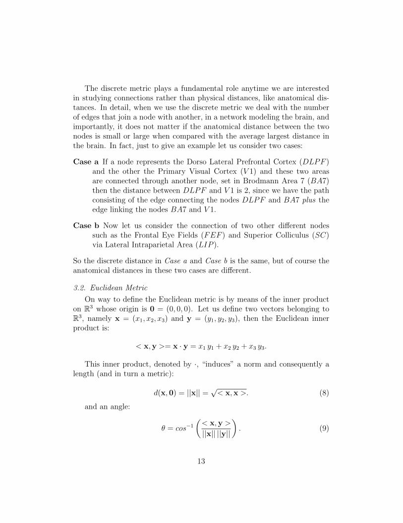
The discrete metric plays a fundamental role anytime we are interestedin studying connections rather than physical distances, like anatomical dis-tances. In detail, when we use the discrete metric we deal with the numberof edges that join a node with another, in a network modeling the brain, andimportantly, it does not matter if the anatomical distance between the twonodes is small or large when compared with the average largest distance inthe brain. In fact, just to give an example let us consider two cases:

Case a If a node represents the Dorso Lateral Prefrontal Cortex (DLPF )and the other the Primary Visual Cortex (V 1) and these two areasare connected through another node, set in Brodmann Area 7 (BA7)then the distance between DLPF and V 1 is 2, since we have the pathconsisting of the edge connecting the nodes DLPF and BA7 plus theedge linking the nodes BA7 and V 1.

Case b Now let us consider the connection of two other different nodessuch as the Frontal Eye Fields (FEF ) and Superior Colliculus (SC)via Lateral Intraparietal Area (LIP ).

So the discrete distance in Case a and Case b is the same, but of course theanatomical distances in these two cases are different.

3.2. Euclidean Metric

On way to define the Euclidean metric is by means of the inner producton R3 whose origin is 0 = (0, 0, 0). Let us define two vectors belonging toR3, namely x = (x1, x2, x3) and y = (y1, y2, y3), then the Euclidean innerproduct is:

< x,y >= x · y = x1 y1 + x2 y2 + x3 y3.

This inner product, denoted by ·, “induces” a norm and consequently alength (and in turn a metric):

d(x,0) = ||x|| =√< x,x >. (8)

and an angle:

θ = cos−1(< x,y >

||x|| ||y||

). (9)

13

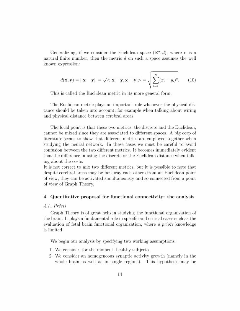
Generalizing, if we consider the Euclidean space (Rn, d), where n is anatural finite number, then the metric d on such a space assumes the wellknown expression:

d(x,y) = ||x− y|| =√< x− y,x− y > =

√√√√ n∑i=1

(xi − yi)2. (10)

This is called the Euclidean metric in its more general form.

The Euclidean metric plays an important role whenever the physical dis-tance should be taken into account, for example when talking about wiringand physical distance between cerebral areas.

The focal point is that these two metrics, the discrete and the Euclidean,cannot be mixed since they are associated to different spaces. A big corp ofliterature seems to show that different metrics are employed together whenstudying the neural network. In these cases we must be careful to avoidconfusion between the two different metrics. It becomes immediately evidentthat the difference in using the discrete or the Euclidean distance when talk-ing about the costs.It is not correct to mix two different metrics, but it is possible to note thatdespite cerebral areas may be far away each others from an Euclidean pointof view, they can be activated simultaneously and so connected from a pointof view of Graph Theory.

4. Quantitative proposal for functional connectivity: the analysis

4.1. Precis

Graph Theory is of great help in studying the functional organization ofthe brain. It plays a fundamental role in specific and critical cases such as theevaluation of fetal brain functional organization, where a priori knowledgeis limited.

We begin our analysis by specifying two working assumptions:

1. We consider, for the moment, healthy subjects.

2. We consider an homogeneous synaptic activity growth (namely in thewhole brain as well as in single regions). This hypothesis may be

14

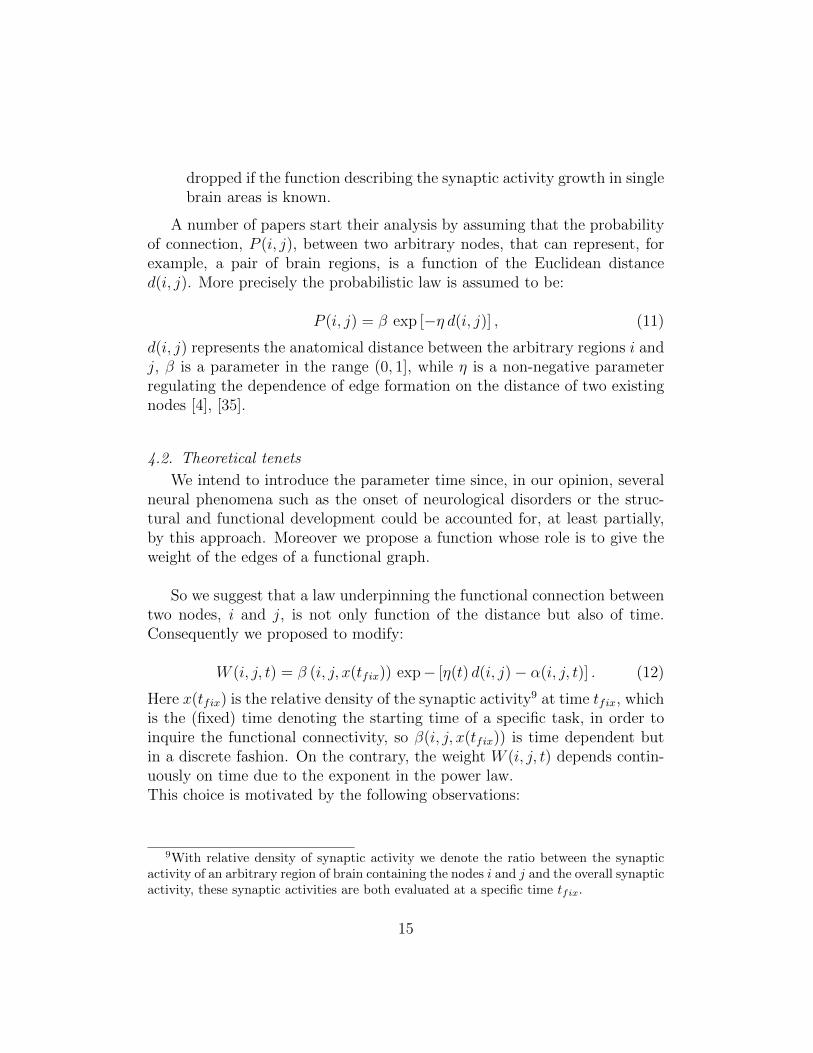
dropped if the function describing the synaptic activity growth in singlebrain areas is known.

A number of papers start their analysis by assuming that the probabilityof connection, P (i, j), between two arbitrary nodes, that can represent, forexample, a pair of brain regions, is a function of the Euclidean distanced(i, j). More precisely the probabilistic law is assumed to be:

P (i, j) = β exp [−η d(i, j)] , (11)

d(i, j) represents the anatomical distance between the arbitrary regions i andj, β is a parameter in the range (0, 1], while η is a non-negative parameterregulating the dependence of edge formation on the distance of two existingnodes [4], [35].

4.2. Theoretical tenets

We intend to introduce the parameter time since, in our opinion, severalneural phenomena such as the onset of neurological disorders or the struc-tural and functional development could be accounted for, at least partially,by this approach. Moreover we propose a function whose role is to give theweight of the edges of a functional graph.

So we suggest that a law underpinning the functional connection betweentwo nodes, i and j, is not only function of the distance but also of time.Consequently we proposed to modify:

W (i, j, t) = β (i, j, x(tfix)) exp− [η(t) d(i, j)− α(i, j, t)] . (12)

Here x(tfix) is the relative density of the synaptic activity9 at time tfix, whichis the (fixed) time denoting the starting time of a specific task, in order toinquire the functional connectivity, so β(i, j, x(tfix)) is time dependent butin a discrete fashion. On the contrary, the weight W (i, j, t) depends contin-uously on time due to the exponent in the power law.This choice is motivated by the following observations:

9With relative density of synaptic activity we denote the ratio between the synapticactivity of an arbitrary region of brain containing the nodes i and j and the overall synapticactivity, these synaptic activities are both evaluated at a specific time tfix.

15

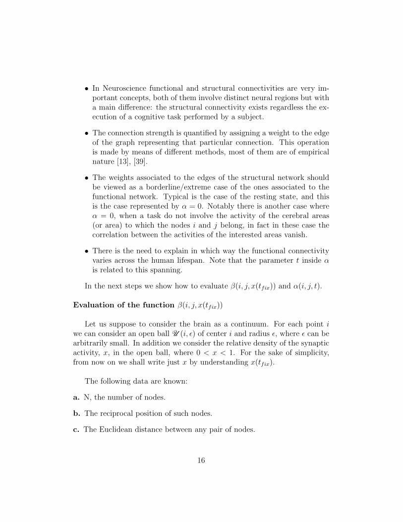
• In Neuroscience functional and structural connectivities are very im-portant concepts, both of them involve distinct neural regions but witha main difference: the structural connectivity exists regardless the ex-ecution of a cognitive task performed by a subject.

• The connection strength is quantified by assigning a weight to the edgeof the graph representing that particular connection. This operationis made by means of different methods, most of them are of empiricalnature [13], [39].

• The weights associated to the edges of the structural network shouldbe viewed as a borderline/extreme case of the ones associated to thefunctional network. Typical is the case of the resting state, and thisis the case represented by α = 0. Notably there is another case whereα = 0, when a task do not involve the activity of the cerebral areas(or area) to which the nodes i and j belong, in fact in these case thecorrelation between the activities of the interested areas vanish.

• There is the need to explain in which way the functional connectivityvaries across the human lifespan. Note that the parameter t inside αis related to this spanning.

In the next steps we show how to evaluate β(i, j, x(tfix)) and α(i, j, t).

Evaluation of the function β(i, j, x(tfix))

Let us suppose to consider the brain as a continuum. For each point iwe can consider an open ball U (i, ε) of center i and radius ε, where ε can bearbitrarily small. In addition we consider the relative density of the synapticactivity, x, in the open ball, where 0 < x < 1. For the sake of simplicity,from now on we shall write just x by understanding x(tfix).

The following data are known:

a. N, the number of nodes.

b. The reciprocal position of such nodes.

c. The Euclidean distance between any pair of nodes.

16

In order to model the brain connectivity, we suggest the introduction ofa synaptic field so defined:

Bi(x) =

∫∫Dj⊂R2

xde(i,j) dDj, (13)

where Dj is the closed subset of R2. It represents a part of the cranial sur-face containing the node j, de(i, j) stands for the Euclidean distance betweentwo nodes i and j, and dDj is the differential surface (or area) element ona surface Dj. If D is the cranial surface, the following relation holds: Dj ⊂ D .

For application purposes we should discretize the equation (13), so ob-taining:

Bi(x) =∑j∈V

xde(i,j). (14)

where V is the set of nodes on the surface D .

We need to introduce a combinatorial evaluation of all synaptic interac-tions between two arbitrary nodes i and j. To that end let us introduce thefollowing polynomial function β(i, j, x):

β (i, j, x) = Bi(x)Bj(x) =∑k∈V

xde(i,k)∑k′∈V

xde(j,k′) (15)

Now we can study the neural network as a graph G = (V ;E), which is anordered pair (V ;E) comprising a set V of vertices or nodes together with aset E of edges. It is worth remarking that once a graph has been introducedin the analysis, then the distance must no longer be regarded as Euclidean(de(i, j)) but only as discrete (d(i, j)). Consequently, in the following, wemust approximate de(i, j) with d(i, j).

de(i, j) ∼ d(i, j) = min l(i, j) = min|N(i, j)| − 1, (16)

where l(i, j) is the characteristic path length between two nodes i and j,min l(i, j) is the shortest path length and min|N(i, j)| is the total number

17

of nodes10 on the shortest path length joining two nodes i and j.

By plugging (16) into (15) we get:

β(i, j, x) =∑k∈V

xd(i,k)∑k′∈V

xd(j,k′) =

(1 + x (deg(i)) + x2N2i + o(x2)

)(1 + x (deg(j)) + x2N2j + o(x2)

),

(17)

where deg(i) is the degree of the node i (similarly for node j), N2i is the num-ber of nodes set at distance 2 from the node i, o(x2) represent the terms thatcould be neglected due to the fact that they are infinitesimal of higher order11.

If no self-loops are considered in the analysis then an additional constraintis demanded: i 6= j, i.e. a node can not interact with itself.In this case equation (17) takes the simplest form:

β(i, j, x) =(x (deg(i)) + x2N2i + o(x2)

) (x (deg(j)) + x2N2j + o(x2)

)∼ (deg(i))(deg(j))x2 + o(x2)

(18)The expression (18) is very similar to the probability of connection of

a new vertex with any other vertex in the network found by Barabasi andReka [7]. It is also quite close to the expression of the coefficient appearingin probability of connection of the economical preferential attachment model,suggested by Vertes, Alexander-Bloch, Gogtay, Giedd, Rapoport and Bull-more [70]. In [7] the exponent γ in the linear case equals to 1, while in thenon-linear case ranges from 1.2 to 4; in [70], γ, the parameter of preferentialattachment, in principle goes from 0 to 6. In particular the authors showedan interesting phase diagram of the economical clustering model, where itappears that most values of two parameters η and γ yield small-world net-works, whereas only high values of γ yield networks with heavy-tailed (skew> 1) degree distribution. The study was done on both healthy volunteers

10The number of nodes (vertices of the graph), which represents the cardinality of V , iscalled the order of the graph and denoted by | V |.

11It is often used the “little-oh” notation in this way: f(x) = g(x) + o(h(x)). This intu-itively means that the error in using g(x) to approximate f(x) is negligible in comparisonto h(x). The little-oh notation was first used by E. Landau in 1909.

18

and participants with childhood onset schizophrenia (COS).

We emphasize that during the discretization of the synaptic field, theinteraction of a node with itself was neglected. This is not a trivial remarksince a node can represent a single neuron as well as cerebral region.So theoretically speaking we could interested in considering also a specialcase: the interaction of a node with itself. In this case it is worth giving somedetails: first, we do not have to set any constraint on vertices so d(i, i) = 0.Second, if i is fixed then d(i, j) = 1 for any j adjacent to i. Third, deg(i) isthe number of nodes, adjacent to i and connected with it.Starting from equation (17) and after a bit of algebraic work, it comes outthat:

β(i, j, x) =(1 + x (deg(i)) + x2N2i + o(x2)

)(1 + x (deg(j)) + x2N2j + o(x2)

)= 1 + (deg(i) + deg(j))x+ (deg(i) deg(j) +N2i +N2j)x

2 + o(x2)(19)

It is interesting to note how the expressions (18) and (19) differ. So in-troducing or not self-looping has great impact on the analysis. It is alsoworth pointing out that generally Neuromathematics disallow self-loops, infact connectivity (and similarly adjacency) matrices are matrices with themain diagonal elements equal to zero and all other elements either positivenumbers or zero.

The evaluation of the function α(i, j, t)

The function α(i, j, t) depends on the specific test submitted to the healthyvolunteer and on age (different stages of life implies different cognitive per-formances).We propose that α(i, j, t) could be represented by the product of two func-tions f(i, j) and g(t):

α(i, j, t) = f(i, j) g(t), (20)

where f(i, j) is strictly related to the task, while g(t) is connected to stage oflife in which the healthy volunteer fall when performing the cognitive task.It is responsible for the changing of the weights associated to the functional

19

edges. We further suggest that f(i, j) is strictly dependent on the correla-tion, derived from the particular task, between the two nodes i and j.

From the available neuroscientific literature there are interesting evi-dences about the evolution of the neural architecture. The following in-formation will be of great help for our (neuro)mathematical analysis.

In the period going from the fetal stage to birth it is not possible to statethat both anatomical and functional connections in the brain can be assumedto exhibit small-world topology [10], [52]12.By studying fetuses of different gestational ages, Thomason et al. [61] bymeans of fMRI analysis revealed that human fetal brain has modular struc-ture, wherein connections are much stronger within, than between, modules,and modules overlap functional systems observed postnatally. This is inagreement with observations in adults, and suggests modularity is an earlyemergent characteristic of the developing brain.In particular, Thomason et al. showed that the brain modularity decreases,and more negative intermodular functional connectivity of the posterior cin-gulate cortex (PCC) occurs with the advancing gestational age [61]. Bymimicking functional principles observed postnatally, these results supportearly emerging capacity for information processing in the human fetal brain.It should be noted that a reduced intermodular connection strength, and highmodularity in younger fetuses, suggests that in early fetal life functional sys-tems are independent, and only with time they begin to collaborate morefully as members of a whole brain system. Prior observations in late child-hood, adolescence, and adulthood, have provided mixed evidence about age-related independence of brain modules. Early research demonstrated thatbrain modules become increasingly independent and separable with advanc-ing age [24], [58].Notably, from birth to 2 years, the human brain undergoes several extraor-dinary changes, including rapid brain volume increases reaching 80 − 90%of adult volume by age 2 [45], rapid elaboration of new synapses [30], veryrapid gray matter volume increasing [28], rapid development of a wide rangeof cognitive and motor functions [33]. In addition, modular organization and

12A small-world organization can support and justify several phenomena and processesproper of brain dynamics, e.g. the segregation and integration of information. In additionthis kind of network represents a trade off between wiring cost minimization and highdynamic complexity. In this sense small-world are “economical” networks.

20

small-world attributes are evident at birth with several important topologicalmetrics increasing monotonically during development. Most significant in-creases of regional nodes occur in the posterior cingulate cortex, which playsa pivotal role in the functional default mode network13 [30].Fransson et al. in their paper [26] provided the possibility to assess whetherthe topographical functional network structure of the infant brain possessessmall-world characteristics, a network property that has previously been de-tected in the adult human brain [65], as well as in children aged from 7 yearsand upward [24], [60].In the childhood the human brain still develops. In this period several mi-crostructural and macrostructural changes take place in order to reshape thebrain’s anatomical networks. Moreover, the relation between these cerebralanatomical networks and the functional networks still evolves, that will leadto the cognitive functions and human behaviors.In the adulthood, it is believed that the brain could develop up to 21-25years. A study, conducted by Sarah-Jayne Blakemore of University CollegeLondon, [14], with brain scans showed that the prefrontal cortex is modifieduntil the age of 30-40 years, and in fact she stated that the prefrontal cortexbegins to develop in the first childhood. Later development continues in lateadolescence and up to 30-40 years, even if the wiring growth is slower thanin childhood. Culture, job career, social relations and environment may playa causal role in the “extra” frontal lobe wiring in adult age. We recall thatthe prefrontal cortex is a part of the brain associated with higher cognitivefunctions, including decision-making, planning and social behavior.Finally it is well known that with aging cerebral performances decrease. Forexample Liu et al. [40] demonstrated age-related changes in the topologicalorganization of large-scale functional brain networks.

13The term “default mode” was first used by Dr. Marcus Raichle in 2001 to describeresting brain function. During the resting state the brain uses hardly less energy than abrain engaged in a task, for example a decision making process. The default mode networkinvolves low frequency oscillations (about one Hertz). This kind of network is most activewhen the brain is at rest, while is deactivated when the brain is focused towards a task.The default mode network includes areas associated with some aspect of internal thought,such as the medial temporal lobe, the medial prefrontal cortex, and the posterior cingulatecortex, as well as the ventral precuneus and parts of the parietal cortex. It is interestingto note that there may be more than one default mode network, so what is known asdefault mode network actually should be thought of as a collection of smaller networks,each dedicated to something which is a bit different than the other.

21

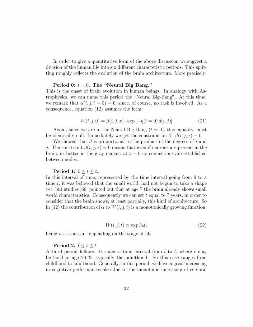
In order to give a quantitative form of the above discussion we suggest adivision of the human life into six different characteristic periods. This split-ting roughly reflects the evolution of the brain architecture. More precisely:

Period 0: t = 0. The “Neural Big Bang.”This is the onset of brain evolution in human beings. In analogy with As-trophysics, we can name this period the “Neural Big-Bang”. At this time,we remark that α(i, j, t = 0) = 0, since, of course, no task is involved. As aconsequence, equation (12) assumes the form:

W (i, j, 0) = β(i, j, x) · exp [−η(t = 0) d(i, j)] (21)

Again, since we are in the Neural Big Bang (t = 0), this equality, mustbe identically null. Immediately we get the constraint on β: β(i, j, x) = 0.

We showed that β is proportional to the product of the degrees of i andj. The constraint β(i, j, x) = 0 means that even if neurons are present in thebrain, or better in the gray matter, at t = 0 no connections are establishedbetween nodes.

Period 1: 0 ≤ t ≤ t.In this interval of time, represented by the time interval going from 0 to atime t, it was believed that the small world, had not begun to take a shapeyet, but studies [60] pointed out that at age 7 the brain already shows smallworld characteristics. Consequently we can set t equal to 7 years, in order toconsider that the brain shows, at least partially, this kind of architecture. Soin (12) the contribution of α to W (i, j, t) is a monotonically growing function:

W (i, j, t) ∝ exph0t, (22)

being h0 a constant depending on the stage of life.

Period 2. t ≤ t ≤ tA third period follows. It spans a time interval from t to t, where t maybe fixed in age 20-25, typically the adulthood. So this case ranges fromchildhood to adulthood. Generally, in this period, we have a great increasingin cognitive performances also due to the monotonic increasing of cerebral

22

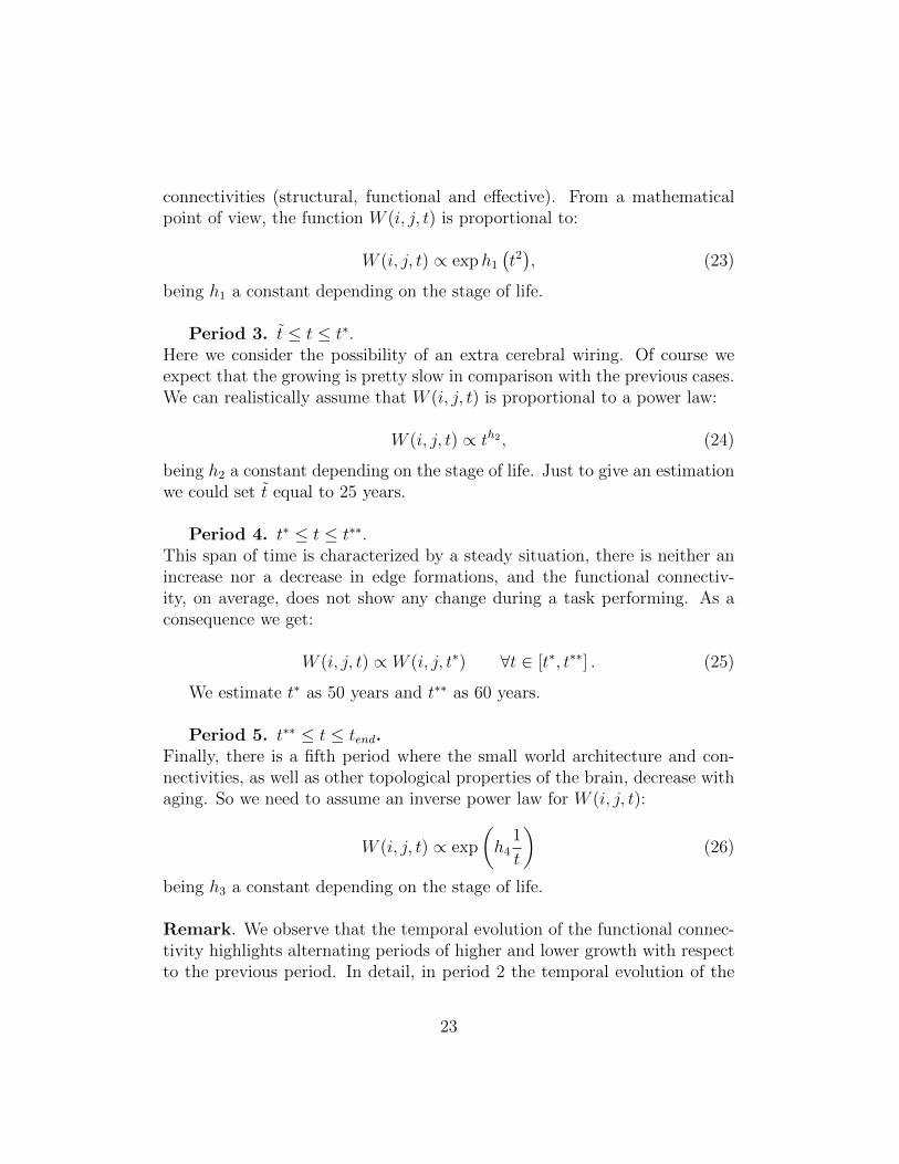
connectivities (structural, functional and effective). From a mathematicalpoint of view, the function W (i, j, t) is proportional to:

W (i, j, t) ∝ exph1(t2), (23)

being h1 a constant depending on the stage of life.

Period 3. t ≤ t ≤ t∗.Here we consider the possibility of an extra cerebral wiring. Of course weexpect that the growing is pretty slow in comparison with the previous cases.We can realistically assume that W (i, j, t) is proportional to a power law:

W (i, j, t) ∝ th2 , (24)

being h2 a constant depending on the stage of life. Just to give an estimationwe could set t equal to 25 years.

Period 4. t∗ ≤ t ≤ t∗∗.This span of time is characterized by a steady situation, there is neither anincrease nor a decrease in edge formations, and the functional connectiv-ity, on average, does not show any change during a task performing. As aconsequence we get:

W (i, j, t) ∝ W (i, j, t∗) ∀t ∈ [t∗, t∗∗] . (25)

We estimate t∗ as 50 years and t∗∗ as 60 years.

Period 5. t∗∗ ≤ t ≤ tend.Finally, there is a fifth period where the small world architecture and con-nectivities, as well as other topological properties of the brain, decrease withaging. So we need to assume an inverse power law for W (i, j, t):

W (i, j, t) ∝ exp

(h4

1

t

)(26)

being h3 a constant depending on the stage of life.

Remark. We observe that the temporal evolution of the functional connec-tivity highlights alternating periods of higher and lower growth with respectto the previous period. In detail, in period 2 the temporal evolution of the

23

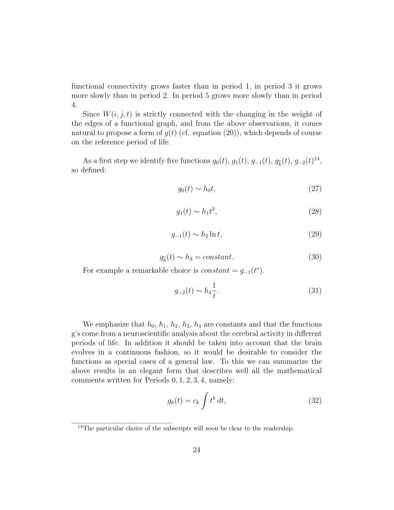
functional connectivity grows faster than in period 1, in period 3 it growsmore slowly than in period 2. In period 5 grows more slowly than in period4.

Since W (i, j, t) is strictly connected with the changing in the weight ofthe edges of a functional graph, and from the above observations, it comesnatural to propose a form of g(t) (cf. equation (20)), which depends of courseon the reference period of life.

As a first step we identify five functions g0(t), g1(t), g−1(t), gk(t), g−2(t)14,

so defined:

g0(t) ∼ h0t, (27)

g1(t) ∼ h1t2, (28)

g−1(t) ∼ h2 ln t, (29)

gk(t) ∼ h3 = constant. (30)

For example a remarkable choice is constant = g−1(t∗).

g−2(t) ∼ h41

t. (31)

We emphasize that h0, h1, h2, h3, h4 are constants and that the functionsg’s come from a neuroscientific analysis about the cerebral activity in differentperiods of life. In addition it should be taken into account that the brainevolves in a continuous fashion, so it would be desirable to consider thefunctions as special cases of a general law. To this we can summarize theabove results in an elegant form that describes well all the mathematicalcomments written for Periods 0, 1, 2, 3, 4, namely:

gk(t) = ck

∫tk dt, (32)

14The particular choice of the subscripts will soon be clear to the readership.

24

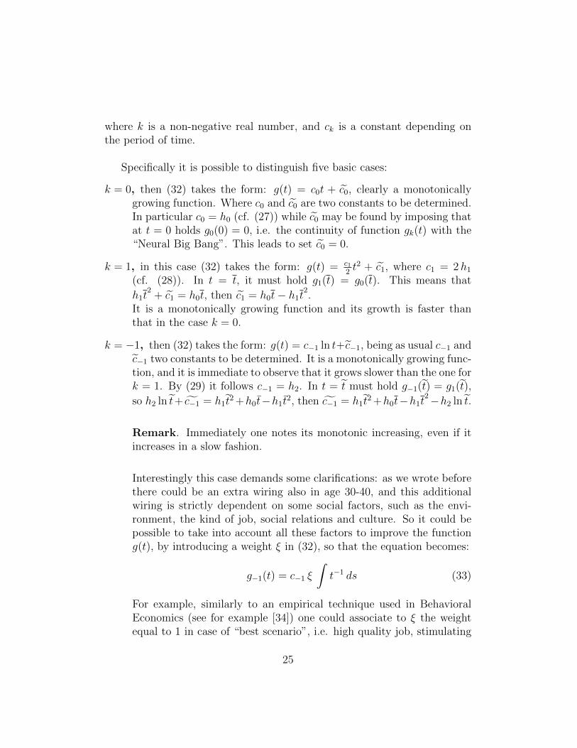
where k is a non-negative real number, and ck is a constant depending onthe period of time.

Specifically it is possible to distinguish five basic cases:

k = 0, then (32) takes the form: g(t) = c0t + c0, clearly a monotonicallygrowing function. Where c0 and c0 are two constants to be determined.In particular c0 = h0 (cf. (27)) while c0 may be found by imposing thatat t = 0 holds g0(0) = 0, i.e. the continuity of function gk(t) with the“Neural Big Bang”. This leads to set c0 = 0.

k = 1, in this case (32) takes the form: g(t) = c12t2 + c1, where c1 = 2h1

(cf. (28)). In t = t, it must hold g1(t) = g0(t). This means that

h1t2

+ c1 = h0t, then c1 = h0t− h1t2.

It is a monotonically growing function and its growth is faster thanthat in the case k = 0.

k = −1, then (32) takes the form: g(t) = c−1 ln t+c−1, being as usual c−1 andc−1 two constants to be determined. It is a monotonically growing func-tion, and it is immediate to observe that it grows slower than the one fork = 1. By (29) it follows c−1 = h2. In t = t must hold g−1(t) = g1(t),

so h2 ln t+ c−1 = h1t2 +h0t−h1t2, then c−1 = h1t

2 +h0t−h1t2−h2 ln t.

Remark. Immediately one notes its monotonic increasing, even if itincreases in a slow fashion.

Interestingly this case demands some clarifications: as we wrote beforethere could be an extra wiring also in age 30-40, and this additionalwiring is strictly dependent on some social factors, such as the envi-ronment, the kind of job, social relations and culture. So it could bepossible to take into account all these factors to improve the functiong(t), by introducing a weight ξ in (32), so that the equation becomes:

g−1(t) = c−1 ξ

∫t−1 ds (33)

For example, similarly to an empirical technique used in BehavioralEconomics (see for example [34]) one could associate to ξ the weightequal to 1 in case of “best scenario”, i.e. high quality job, stimulating

25

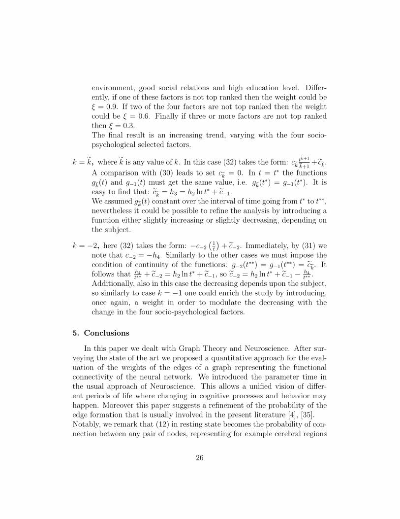
environment, good social relations and high education level. Differ-ently, if one of these factors is not top ranked then the weight could beξ = 0.9. If two of the four factors are not top ranked then the weightcould be ξ = 0.6. Finally if three or more factors are not top rankedthen ξ = 0.3.The final result is an increasing trend, varying with the four socio-psychological selected factors.

k = k, where k is any value of k. In this case (32) takes the form: cktk+1

k+1+ ck.

A comparison with (30) leads to set ck = 0. In t = t∗ the functionsgk(t) and g−1(t) must get the same value, i.e. gk(t

∗) = g−1(t∗). It is

easy to find that: ck = h3 = h2 ln t∗ + c−1.We assumed gk(t) constant over the interval of time going from t∗ to t∗∗,nevertheless it could be possible to refine the analysis by introducing afunction either slightly increasing or slightly decreasing, depending onthe subject.

k = −2, here (32) takes the form: −c−2(1t

)+ c−2. Immediately, by (31) we

note that c−2 = −h4. Similarly to the other cases we must impose thecondition of continuity of the functions: g−2(t

∗∗) = g−1(t∗∗) = ck. It

follows that h4

t∗∗+ c−2 = h2 ln t∗ + c−1, so c−2 = h2 ln t∗ + c−1 − h4

t∗∗.

Additionally, also in this case the decreasing depends upon the subject,so similarly to case k = −1 one could enrich the study by introducing,once again, a weight in order to modulate the decreasing with thechange in the four socio-psychological factors.

5. Conclusions

In this paper we dealt with Graph Theory and Neuroscience. After sur-veying the state of the art we proposed a quantitative approach for the eval-uation of the weights of the edges of a graph representing the functionalconnectivity of the neural network. We introduced the parameter time inthe usual approach of Neuroscience. This allows a unified vision of differ-ent periods of life where changing in cognitive processes and behavior mayhappen. Moreover this paper suggests a refinement of the probability of theedge formation that is usually involved in the present literature [4], [35].Notably, we remark that (12) in resting state becomes the probability of con-nection between any pair of nodes, representing for example cerebral regions

26

[35], [70], despite the fact that in general W (i, j, t) is not a distribution ofprobability. If we are not in the resting state, W (i, j, t) changes the functionalconnectivity depending on the specific task submitted to the volunteer.Interestingly, in this approach there is not any experimental constraint so itmay be applied to different brain survey techniques, e.g. fMRI, MEG, EEG,etc.The function W (i, j, t) could contribute to shed more light on understand-ing how, in different periods of life, the functional graph and its topologicalcharacteristics change.

References

[1] Achard S, Bullmore ET (2007). Efficiency and cost of economical brainfunctional networks. PLoS Comput Biol 3:e17.

[2] Agosta, F. et al. (2013) Brain network connectivity assessed using graphtheory in frontotemporal dementia. Neurology 81, 134143

[3] Alexander-Bloch, A.F. et al. (2010). Disrupted modularity and local con-nectivity of brain functional networks in childhood-onset schizophrenia.Front. Syst. Neurosci. 4, 147.

[4] Alexander-Bloch, A.F. et al. (2013). The anatomical distance of func-tional connections predicts brain network topology in health andschizophrenia. Cereb. Cortex 23, 127138.

[5] Alonso-Solis, A. et al. (2013). Altered default network resting statefunctional connectivity in patients with a first episode of psychosis.Schizophr. Res. 139, 1318. CHI 2013: 483-492.

[6] Amaral, L.A.N., Scala, A., Barthelemy, M., Stanley, H.E. (2000). Classesof small-world networks. Proc. Natl. Acad. Sci. U. S. A. 97, 11149-11152(2000).

[7] Barabasi, A.-L., Reka, A. (1999). Emergence of Scaling in Random Net-works. Science 15 October 1999: Vol. 286 no. 5439 pp. 509-512.

[8] Barabasi, Oltvai, Z.N. (2004). Network biology: understanding the cell’sfunctional organization. Nat Rev Genet 5, 101-113

27

[9] Barthelemy, M. (2004). Betweenness centrality in large complex net-works. Eur. Phys. J. B 38, 163-168.

[10] Bassett, D.S. and Bullmore, E.T. (2006). Small world brain networks.The Neuroscientist. Vol. 12, Number 6, 2006.

[11] Bassett, Bullmore, Verchinski, Mattay, Weinberger, Meyer-Lindenberg(2008). Hierarchical Organization of Human Cortical Networks in Healthand Schizophrenia.

[12] Bassett, D.S. and Bullmore, E.T. (2009). Human brain networks inhealth and disease. Curr. Opin. Neurol. 22, 340347.

[13] Betzel, R.F., Byrge, L., He, Y., Goni, J., Zuo, X., Sporns, O. (2014).Changes in structural and functional connectivity among resting-statenetworks across the human lifespan. NeuroImage 102 (2014) 345357.

[14] http://www.ted.com/talks/sarah_jayne_blakemore_the_

mysterious_workings_of_the_adolescent_brain#

[15] Bollobas B. (1985). Random graphs. London: Academic.

[16] Bonacich, P. (1972). Factoring and weighting approaches to clique iden-tification. Journal of Mathematical Sociology, 2, 113-120.

[17] Buckley, F., Harary, F. (1990). Distance in Graphs. Addison-Wesley,Boston.

[18] Buckner, R.L. et al. (2009). Cortical hubs revealed by intrinsic func-tional connectivity: mapping, assessment of stability, and relation toAlzheimer’s disease. J. Neurosci. 29, 18601873.

[19] Bullmore and Sporn (2009). Complex Brain Networks Graph TheoreticalAnalysis Of Structural and Functional Systems.

[20] Bullmore, E. and Sporns, O. (2012). The economy of brain networkorganization. Nat. Rev. Neurosci. 13, 336349.

[21] Choromanski, K., Matuszak, M., Miekisz, J. (2013). Scale-Free Graphwith Preferential Attachment and Evolving Internal Vertex Structure.J. Stat. Phys. DOI 10.1007/s10955-013-0749-1.

28

[22] de Haan, W. et al. (2013). Activity dependent degeneration explains hubvulnerability in Alzheimers disease. PLoS Comput. Biol. 8, e1002582.

[23] Dulio, P., Pannone, V. (2013). Iterated Joining of Rooted Trees. Graphsand Combinatorics (2013) 29:12871304.

[24] Fair D.A., Cohen A.L., Power J.D., Dosenbach N.U., Church J.A., et al.(2009). Functional brain networks develop from a “local to distributed”organization. PLoS Comput Biol 5: 114.

[25] Fornito, A. et al. (2012). Schizophrenia, neuroimaging and connectomics.Neuroimage 62, 22962314.

[26] Fransson, P., Aden, U., Blennow, M., and Lagercrantz, H. (2011). TheFunctional Architecture of the Infant Brain as Revealed by Resting-StatefMRI. Cerebral Cortex January 2011;21:145-154.

[27] Friston, K.J. (1994). Functional and Effective Connectivity in Neu-roimaging: A Synthesis. Human Brain Mapping 2:56-78.

[28] Gilmore JH, Lin W, Prastawa MW, Looney CB, Vetsa YS, KnickmeyerRC, Evans DD, Smith JK, Hamer RM, Lieberman JA et al. (2007). Re-gional gray matter growth, sexual dimorphism, and cerebral asymmetryin the neonatal brain. J Neurosci. 28:17891795.

[29] Greicius, M.D. et al. (2004). Default-mode network activity distinguishesAlzheimers disease from healthy aging: evidence from functional MRI.Proc. Natl. Acad. Sci. U.S.A. 101, 46374642

[30] Huang et al. (2013). Development of Human Brain StructuralNetworks Through Infancy and Childhood. Cerebral Cortexdoi:10.1093/cercor/bht335.

[31] Humphries M.D., Gurney, K., Prescott, T.J. (2006). The brainstemreticular formation is a small-world, not scale-free, network. Proc BiolSci 273:503511.

[32] Jeong H., MasonS.P., Barabaasi A.-L., and Oltvai Z.N.(2001). Lethalityand centrality in protein networks. Nature 411, 41 (2001).

[33] Kagan J, Herschkowitz N. 2005. A young mind in a growing brain. Mah-wah: Erlbaum Associates.

29

[34] Kahneman, D. (2011). Thinking, Fast and Slow. Farrar, Straus andGiroux.

[35] Kaiser, M.,Hilgetag, C.C. (2008). Spatial Growth of Real-world Net-works. Phys. Rev. E 69 (3) 2004

[36] Karbasforoushan, H. and Woodward, N.D. (2013) Resting-state net-works in schizophrenia. Curr. Top. Med. Chem. 12, 24042414

[37] Lang, Tome, Keck, Gorriz-Saez, and Puntonet. (2012). Brain Connec-tivity Analysis, A Short Survey, Structural functional and effective con-nectivity. Computational Intelligence and Neuroscience Volume 2012,Article ID 412512, 21 pages.

[38] Latora V, Marchiori M (2001). Efficient behavior of small-world net-works. Phys Rev Lett 87:198701.

[39] Liu, Y., Yu, C., Zhang, X., Liu, J., Duan, Y., Alexander-Bloch,A.F., Liu, B., Jiang, T., and Bullmore, E. (2013). Impaired Long Dis-tance Functional Connectivity and Weighted Network Architecture inAlzheimer’s Disease. Cereb. Cortex 10.1093/cercor/bhs410.

[40] Liu Z, Ke L, Liu H, Huang W, Hu Z (2014). Changes in TopologicalOrganization of Functional PET Brain Network with Normal Aging.PLoS ONE 9(2): e88690. doi:10.1371/journal.pone.0088690.

[41] Lynall, M.E. et al. (2010). Functional connectivity and brain networksin schizophrenia. J. Neurosci. 30, 94779487.

[42] Newman, M. E. J. (2003). The structure and function of complex net-works. SIAM Rev. 45, 167256.

[43] Newman, M. E. J. (2006). Modularity and community structure in net-works. PNAS, vol. 103, n 23, 2006, pp. 85778582.

[44] Onnela, J.-P., Saramaki, J., Hyvonen, J., Szabo, G., Lazer, D.,Kaski, K., Kertesz, K., and Barabasi, A.-L. (2007). Structure and tiestrengths in mobile communication networks. Proceedings of the Na-tional Academy of Sciences 104 (18): 73327336.

30

[45] Pfefferbaum A, Mathalon DH, Sullivan EV, Rawles JM, Zipursky RB,Lim KO. 1994. A quantitative magnetic-resonance-imaging study ofchanges in brain morphology from infancy to late adulthood. Arch Neu-rol. 51:874887.

[46] Raj, A. et al. (2012). A network diffusion model of disease progressionin dementia. Neuron 73, 12041215.

[47] Ravasz, E. and Barabaasi,A.-L. (2003). Hierarchical organization incomplex networks. Phys. Rev. E 67, 026112 (2003).

[48] Seeley, W.W. et al. (2009). Neurodegenerative diseases target largescalehuman brain networks. Neuron 62, 4252.

[49] Shi, F. et al. (2012). Altered structural connectivity in neonates at ge-netic risk for schizophrenia: a combined study using morphological andwhite matter networks. Neuroimage 62, 16221633.

[50] Shi, F. et al. (2013). Altered modular organization of structural corticalnetworks in children with autism. PLoS ONE 8, e63131.

[51] Sporns, O., Tononi, G., Edelman, G.M. Theoretical Neuroanatomy: Re-lating Anatomical and Functional Connectivity in Graphs and CorticalConnection Matrices (2000). Cereb. Cortex 10 (2): 127-141.

[52] Sporns, Chialvo, Kaiser, Hilgetag. (2004). Organization, developmentand function of complex brain networks.TRENDS in Cognitive SciencesVol.8 No.9 September 2004.

[53] Sporns, O., Kotter, R. Motifs in Brain Networks (2004). PLoS Biol2(11): e369. doi:10.1371/journal.pbio.0020369. Academic Editor: KarlJ.

[54] Sporns, O., Honey, C. J., and Kotter, R. Identification and classificationof hubs in brain networks (2007). PLoS ONE, vol. 2, no. 10, Article IDe1049.

[55] Sporns, O. Networks of the Brain (2010). The MIT press.

[56] Sporns (2011). The non-random brain, efficiency, economy, and complexdynamics. Frontiers in Computational Neuroscience. 2011; 5:5.

31

[57] Stam, C.J. et al. (2009). Graph theoretical analysis of magnetoen-cephalographic functional connectivity in Alzheimer’s disease. Brain132, 213224.

[58] Stevens, M.C., Pearlson, G.D., Calhoun, V.D. (2009). Changes in theinteraction of resting-state neural networks from adolescence to adult-hood. Hum Brain Mapp 30: 23562366.

[59] Supekar, K. et al. (2008). Network analysis of intrinsic functional brainconnectivity in Alzheimer’s disease. PLoS Comput. Biol. 4, e1000100.

[60] Supekar, K., Musen, M., Menon, V. (2009). Development of large-scalefunctional brain networks in children. PLoS Biol. 7:e1000157.

[61] Thomason, M.E., Brown, J.A., Dassanayake, M.T., Shastri, R.,Marusak, H.A., et al. (2014). Intrinsic Functional Brain ArchitectureDerived from Graph Theoretical Analysis in the Human Fetus. PLoSONE 9(5): e94423. doi:10.1371/journal.pone.0094423.

[62] Turner, M.R. et al. (2011). Towards a neuroimaging biomarker for amy-otrophic lateral sclerosis. Lancet Neurol. 10, 400403.

[63] Verstraete, E. et al. (2010). Motor network degeneration in amyotrophiclateral sclerosis: a structural and functional connectivity study. PLoSONE 5, e13664.

[64] Verstraete, E. et al. (2013). Structural brain network imaging showsexpanding disconnection of the motor system in amyotrophic lateralsclerosis. Hum. Brain Mapp. http://dx.doi.org/10.1002/hbm.22258.

[65] van den Heuvel, M.P., Stam, C.J., Boersma, M., Hulshoff Pol, H.E.(2008). Smallworld and scale-free organization of voxel-based resting-state functional connectivity in the human brain. Neuroimage. 43:528-539.

[66] van den Heuvel, M.P. et al. (2010). Aberrant frontal and temporal com-plex network structure in schizophrenia: a graph theoretical analysis. J.Neurosci. 30, 1591515926.

[67] van den Heuvel et al. (2012). High-cost, high-capacity backbone forglobal brain communication. 1137211377, PNAS, July 10, 2012, vol.109, no. 28.

32

[68] van den Heuvel and Olaf Sporns (2013). Network hubs in the humanbrain. 2013. Trends in Cognitive Sciences, December 2013, Vol.17, No.12.

[69] van den Heuvel, M.P. et al. (2013). Abnormal rich club organizationand functional brain dynamics in schizophrenia. JAMA Psychiatry 70,783792.

[70] Vertesa, P.E., Alexander-Bloch, A.F., Gogtay, N., Gieddb, J.N.,Rapoport, J.L. and Edward T. Bullmore (2012). Simple models of hu-man brain functional networks. PNAS, April 2012, vol.109, no. 15, 5860-5873.

[71] Watts, D. J., and Strogatz, S. H. (1998). Collective dynamics of “small-world” networks. Nature 393, 440442.

[72] Yu, Q. et al. (2013). Disrupted correlation between low frequency powerand connectivity strength of resting state brain networks in schizophre-nia. Schizophr. Res. 143, 165171.

[73] Zalesky, A. et al. (2011). Disrupted axonal fiber connectivity inschizophrenia. Biol. Psychiatry 69, 8089.

33