Sylvester rank functions, epic division rings and the strong Atiyah conjecture

for locally indicable groups

´ Diego Lopez Alvarez

A thesis submitted for the degree of Doctor in Mathematics.

Supervised by: Andrei Jaikin Zapirain

Madrid, 2021

FUNCIONES DE RANGO DE SYLVESTER, ANILLOS DE ´ ´ DIVISION EPICOS Y LA CONJETURA FUERTE DE

ATIYAH PARA GRUPOS LOCALMENTE INDICABLES

A lo largo de la tesis, consideramos cuestiones relacionadas con embed-dings de dominios no conmutativos en anillos de division.

Por un lado, tratamos el problema de existencia de tales embeddings para anillos de grupo K[G] donde K es un subcuerpo del cuerpo de numeros complejos C y G es un grupo localmente indicable (por ejemplo, un grupo libre de torsion que admite una presentacion con solo una relacion). Estos grupos forman una subfamilia de grupos ordenables a izquierda, y por tanto este problema es un caso particular del problema de embedding de Malcev.

En este sentido, la conjetura fuerte de Atiyah para estos anillos de grupo, motivacion original y principal de la tesis, propone un candidato a anillo de division que contiene a K[G], este es, la clausura de division de K[G] en el anillo clasico de cocientes U(G) del algebra´ de grupos de von Neumann N (G). En el resultado principal (trabajo conjunto con A. Jaikin-Zapirain) probamos que la conjetura fuerte de Atiyah se satisface en este caso y que, ademas, el anillo de division resultante puede ser identificado unıvocamente mediante una propiedad universal. Los resultados y metodos asociados nos permiten probar posteriormente otras conjeturas relacionadas, como por ejemplo una version de la conjetura de aproximacion de Luck para grupos virtualmente localmente indicables.

Por otro lado, consideramos la nocion de universalidad de un anillo de division. Para un anillo R, un anillo de division universal de fracciones es un anillo de division que contiene a y esta generado por R como anillo de division, y en el que podemos invertir “la mayor cantidad de matrices” posi-ble sobre R. A este respecto, los dominios de Sylvester y pseudo-Sylvester son anillos que admiten un anillo de division universal de fracciones sobre el que toda matriz se vuelve invertible a menos que haya una obstruccion “obvia” que lo impida.

En un trabajo conjunto con F. Henneke probamos que los productos cruzados de la forma E ∗ G, donde E es un anillo de division y G es libre-por-{cıclico infinito}, son siempre dominios pseudo-Sylvester, y exploramos la situacion mas general de productos cruzados F ∗ Z de un anillo de ideales libres (fir) F y el anillo de enteros Z.

Durante toda la tesis, la teorıa de funciones de rango de Sylvester pro-porciona al mismo tiempo un lenguaje homogeneo y una herramienta para abordar los problemas considerados. Por ello, analizamos en mayor profun-didad el espacio de las funciones de rango de Sylvester que pueden definirse sobre ciertas familias de anillos, tales como los dominios de Dedekind o una subfamilia de anillos de polinomios de Laurent asimetricos con coeficientes en un anillo de division (trabajo conjunto con A. Jaikin-Zapirain).

A mi familia y a Rocıo

Agradecimientos

Ningun camino se recorre solo, y son muchas las personas que fortuita y afortunadamente me han permitido compartir consigo parte del largo trecho que me ha llevado a escribir estas paginas, que cuentan mejor lo que he sido y lo que soy que el resto de la tesis. Y aunque quiza no es lo suyo comenzar unos agradecimientos con una disculpa, siento mucho la incapacidad para reflejar con estas pocas palabras lo que ha significado tenerlos a mi lado.

La primera persona a la que debo agradecer que esto sea posible es, sin duda alguna, Andrei. Gracias por brindarme la oportunidad de aprender contigo, y gracias por toda la ayuda a lo largo de estos poco mas de 4 anos, que en varias ocasiones ha trascendido a lo puramente academico. Sabes que no escribirıa esto si no lo pensara, pero a tu lado he entendido lo que hace a un investigador. Muchas gracias, de corazon.

Aprovechando la oportunidad, agradezco a los profesores que me han alentado a seguir este camino. Muchısimas gracias, Vicente y Arturo, por inculcarme la fascinacion por las Matematicas en el colegio y el instituto. Muchısimas gracias, Margarita, porque si no te hubiera tenido como tutora (no oficial) no habrıa sabido seguir adelante tras la entrada en la universidad. Muchısimas gracias, Mercedes, por ensenarme a disfrutar

´ el Algebra, porque seas o no consciente de ello inspiraste a muchos con tu pasion por tu trabajo. Y muchısimas gracias tambien a Luis Felipe y Fernando, que durante el Master y la Escuela JAE, respectivamente, me guiaron durante los primeros pasos por la investigacion. Junto con ellos, agradezco muchısimo a Yago y a Javier A. su acogida dentro del grupo; desconocen lo que un simple gesto puede significar para alguien.

Me gustarıa agradecer tambien a Javier Sanchez, cuya tesis ha sido ejemplo e in-spiracion de la que aquı se presenta, tanto por el contenido como por el mimo que se palpa al leerla. Tambien quiero agradecerle su labor como lector. In this regard, I would like to thank Hanfeng Li, whose thorough reading and comments on the thesis have helped me a lot in improving the outcome. I would also like to thank him and Lukasz Grabowski for writing the international reports to the thesis.

Ahora, comenzando por el principio, gracias a mis amigos de toda la vida, a Raquel, a Carlos, a mis companeros de clase en el colegio e instituto, a la gente de la plaza de Realejo Alto y a mis companeros del OsusonaTM . Aunque en algunos casos nuestros caminos se hayan alejado un poco con el paso del tiempo, me resulta imposible escribir unos agradecimientos que no los incluyan. Gracias por los mejores anos de mi vida, cuando nuestra mayor preocupacion era saber quien traerıa la pelota el sabado.

I

II

Gracias tambien a todas aquellas personas con las que compartı gran parte de la etapa universitaria. En especial a Luis M., Misael, Yeray, Aythami y Juan Jesus, por compartir sus locuras conmigo y permitirme compartir las mıas. El camino se hace mas ligero cuando vas bien acompanado, y no lo habrıa disfrutado ni la mitad si no me hubiera topado con ustedes.

Muchısimas gracias a todos los que, entre la UAM y el ICMAT, han aliviado las cargas de este viaje, que como todo viaje largo ha tenido sus momentos crıticos.

No puedo empezar de otra manera que no sea dando las gracias a los companeros del despacho 513. Marta, durante muchos anos has sido la voz de mi conciencia, ası que gracias por tu insistencia, tu ´ Sinceramente, he conocido animo y tu apoyo con todo. a muy pocas personas como tu en este tiempo, y haber coincidido contigo tantos anos y en tantos sitios solo me hace pensar en la suerte que me ha acompanado siempre. Carlos, ya en aquel momento se podıan ver tus aptitudes de padre y docente. Gracias por haberme prestado atencion cuando mas aislado me sentıa en la investigacion, y por haberme echado un cable cuando creıa no entender nada. Ale, Fran, aunque finalmente pudimos compartir poco tiempo como companeros de despacho por causas inesperadas, agradecı muchısimo tenerlos allı; devolvieron al 513 la vida que perdıa a medida que se iba quedando vacıo.

Agradezco tambien a Adri, doctorando Prime y cafetero premium. Gracias por todas esas charlas de cafe a primera hora de la manana que, durante mucho tiempo, se con-virtieron en lo personal en la mayor motivacion del dıa. A Julio, al que de alguna manera siento mi hermano de tesis y con el que he compartido muchos momentos de frustracion, de charlas, de congresos y de marrones varios (gracias a los cuales sabemos preparar y servir cantidades industriales de cafe, te y pastas). Espero que algun dıa te des cuenta de lo que vales en realidad. A Luis A., al que me gusta afirmar que no soporto cuando en realidad pienso que hace falta mas gente como el por el mundo. Eres de las personas que hacen grupo, que acogen y hacen sentir comoda a la gente cuando aun esta desubicada, pero negare rotundamente que he escrito esto si me preguntan.

Y por supuesto, le doy las gracias a todas las personas que han formado parte de este camino a lo largo de los anos: a Jaime, Bea B., Bea P., Raquel, Florian, Diego M., Hang Lu, Manuel, Nikita, Dani, Marcos, Irina, Iason, Glenier, Sauli, Leyter, Martı, Jose, a mi hermano mayor de tesis Javier, y al menor Jan, y a las incorporaciones mas recientes Celia, Dani, Mikel e Ismael.

I would also like to thank all the people who tried hard to make me feel like home during my stay at the MPIM in Bonn. Wolfgang, thank you for giving me the opportunity to be there, and Benny, Johanna, Elia, Claudio, I am sincerely grateful for letting me spend this adventure with you. Fabian, I am not grateful but indebted to you. You, more than anyone, experienced by my side the tough part of the stay, and there is absolutely nothing I can write here to express how much I owe you for that. You have not only been a fantastic host and office mate during those three months and a great collaborator after them, but a friend to me. I wish you the best luck someone can wish for, because you do deserve it. Thank you.

Tampoco me puedo dejar atras a Diego A. y Tania, que me han acogido siempre en

III

su casa, primero en Madrid y luego en Bonn. Hemos sido companeros de clase, de piso, de despacho,. . . y en todas las ocasiones me han tendido su mano. Muchısimas gracias. Y gracias tambien a Vıctor, con quien he convivido en Madrid la gran mayorıa de estos anos, confinamiento incluido, y que es excepcional como companero y persona.

Y he dejado para el final a las personas a las que mas debo, por aguantarme desde que no tenıa idea alguna hasta que se me ocurrio la “brillante” idea de aventurarme con la tesis: mi familia. Le doy las gracias a mi tıo Javi, que siempre me infundi´ ´´ o animos para seguir este camino, a Marian y a mis abuelos Domingo y Mercedes. A mi hermano Enri, que como hermano mayor ha tenido que abrir camino y, por que no decirlo, sacarme las castanas del fuego en mas de una ocasion antes y despues de la etapa universitaria, y a su pareja Laura, a quien le ha tocado la ardua tarea de meterlo en vereda. Y por supuesto, a mis padres, Enrique y Candelaria, que son quienes me han traıdo hasta aquı y han puesto todos los medios y todo el apoyo para guiarme hasta lo que soy. En especial querrıa agradecerle a mi madre, que siempre se ha partido el lomo para darnos el empujon necesario para sacarnos adelante, y que aun cree que lo que hace por el resto de la familia no es suficiente.

A Lana y a Mimi, mis dos pequenas y el amor mas puro, incondicional e inocente que uno puede recibir. Lana, me habrıa gustado que pudieras seguirme hasta este momento, pero aunque no haya sido posible siempre te llevo conmigo. Mimi, gracias por devolverme la sonrisa, por ser mi companera de juegos y por sacarme de paseo siempre que me ves. Aunque ninguna de las dos sabrıa leer estas paginas, me gusta pensar que entienden por que forman parte de ellas.

Y finalmente quiero dar las gracias a Rocıo. Son tantas las decisiones difıciles que hemos debido tomar a lo largo de estos ´ nos, incluso en la distancia, que ya niultimos a˜ imagino ni entiendo una vida sin ti como companera de viaje. Gracias por estar ahı, porque en ocasiones saber que cuento contigo es lo que me mantiene en pie. Ojala la conclusion de este capıtulo en mi vida sea el inicio de nuestra vida juntos.

En definitiva, gracias a todos por todo. Cuanto mas escribo y recuerdo mas consciente soy de que sin su companıa este trayecto no habrıa cobrado sentido. Cruzo los dedos por no haberme olvidado de nadie, y si es ası, disculpame, tambien va por ti. GRACIAS.

Contents

Introduccion y conclusiones iii Resumen y conclusiones por capıtulo . . . . . . . . . . . . . . . . . . . . . . . . ix

Introduction and conclusions xvii Summary and conclusions by chapter . . . . . . . . . . . . . . . . . . . . . . . . xxiii

1 Rank functions 1 1.1 Inner and stable rank over a stably finite ring . . . . . . . . . . . . . . . . 3

1.2 Sylvester rank functions . . . . . . . . . . . . . . . . . . . . . . . . . . . . 9

1.3 Rank functions and von Neumann regular rings . . . . . . . . . . . . . . . 18

1.4 Extending rank functions . . . . . . . . . . . . . . . . . . . . . . . . . . . 24

1.5 The natural transcendental extension of exact ranks . . . . . . . . . . . . 39

2 The space of Sylvester rank functions 49 2.1 The space P(R) and first examples . . . . . . . . . . . . . . . . . . . . . . 50

2.2 Left artinian primary rings . . . . . . . . . . . . . . . . . . . . . . . . . . 60

2.3 Sylvester rank functions on a Dedekind domain . . . . . . . . . . . . . . . 64

2.4 Krull dimension and simple left noetherian rings . . . . . . . . . . . . . . 69

2.5 Skew Laurent polynomials over division rings . . . . . . . . . . . . . . . . 71

3 Epic division rings and pseudo-Sylvester domains 81 3.1 Universal localization and epic division rings. Universal division rings of

fractions . . . . . . . . . . . . . . . . . . . . . . . . . . . . . . . . . . . . . 82

3.2 Sylvester and pseudo-Sylvester domains . . . . . . . . . . . . . . . . . . . 90

3.3 Division and rational closures . . . . . . . . . . . . . . . . . . . . . . . . . 97

3.4 Crossed products, locally indicable groups and Hughes-free division rings of fractions . . . . . . . . . . . . . . . . . . . . . . . . . . . . . . . . . . . 103

3.5 The crossed product F ∗Z of a fir F and Z . . . . . . . . . . . . . . . . . . 125

4 The strong Atiyah conjecture 137 4.1 ∗-regular and epic ∗-regular rings . . . . . . . . . . . . . . . . . . . . . . . 138

4.2 U(G) and the strong Atiyah conjecture . . . . . . . . . . . . . . . . . . . . 157

4.3 Rational semirings and the notion of complexity . . . . . . . . . . . . . . 169

4.4 The strong Atiyah conjecture for locally indicable groups . . . . . . . . . 193

i

ii Contents

5 Related conjectures and results 201 5.1 Other directly related conjectures . . . . . . . . . . . . . . . . . . . . . . . 201 5.2 Luck’s approximation in the space of marked groups . . . . . . . . . . . . 210 5.3 On the universality of the Hughes-free division ring . . . . . . . . . . . . . 236

Bibliography 243

Introduccion y conclusiones

Aunque quiza, si hablamos del desarrollo cronologico de la tesis, esto no sea del todo pre-ciso, las principales motivaciones de este trabajo pueden explicarse desde la perspectiva de un primer curso en algebra lineal y teorıa de anillos.

A este respecto, una de las primeras estructuras algebraicas con la que nos topamos al iniciarnos en ambos campos es la de cuerpo (conmutativo), siendo Q, R o C los ejemplos mas habituales. El hecho de que todo elemento no nulo en un cuerpo K admite un inverso multiplicativo y de que todo K-modulo (es decir, espacio vectorial) finitamente generado es libre con un numero finito fijo de elementos en cualquier base, hace de los cuerpos un contexto ideal en el que trabajar.

Como consecuencia, dado un anillo conmutativo R, es natural preguntarse si R puede ser identificado como subanillo de algun cuerpo, de manera que aun podamos utilizar la maquinaria desarrollada en algebra lineal y heredemos de paso algunas de sus propiedades basicas. Por ejemplo, el anillo de los numero enteros, Z, es de manera natural un subanillo de Q, R y C. Ası pues, podrıamos plantearnos, quiza de manera aun imprecisa, las siguientes cuestiones:

1. Dado un anillo conmutativo R, ¿existe un cuerpo K del que R sea subanillo?

2. Si para un anillo R concreto la respuesta a la primera pregunta es afirmativa, ¿es el cuerpo K “unico”?

3. Si, tras precisar el significado de unicidad, la respuesta a la segunda pregunta es negativa, ¿existe alguna manera de caracterizar (alguno de) los cuerpos de los que R es subanillo? ¿Existe alguno que sea “universal” en algun sentido?

Tratemos de puntualizar y responder apropiadamente estas preguntas en el caso con-mutativo. Un obstaculo insalvable para la existencia de un cuerpo K como en 1. es la presencia de divisores de cero no triviales en R, es decir, de elementos no nulos a y b tales que ab = 0 en R. No obstante, si no estamos en esta situacion, o equivalentemente, cuan-do R es un dominio, sabemos que podemos construir el denominado cuerpo de fracciones de R, un cuerpo cuya descripcion recuerda a la de Q con respecto a Z, en el sentido de que sus elementos son fracciones de elementos de R con denominador no nulo junto con las operaciones usuales. Por tanto, la respuesta a la primera pregunta es afirmativa si y solo si R es un dominio.

iii

!/

iv

Con respecto a la segunda pregunta, ya hemos mencionado un ejemplo en el que con-tamos con multiples opciones entre las que elegir (de hecho, una cantidad no numerable de ellas si consideramos extensiones de cuerpos de Q), pero algunas de ellas son o bien muy “grandes” o bien muy “complicadas” en comparacion con el anillo original Z. En este sentido, la construccion de Q a partir de Z lo hace quiza el cuerpo mas “sencillo” de

1 entre todos ellos: simplemente anadimos un inverso para todo entero no nulo b y losb elementos estrictamente necesarios (fracciones b

a) para dotar de una estructura de anillo al nuevo conjunto obtenido. Decimos en este caso que Q esta generado por Z como cuer-po, puesto que todo numero racional puede obtenerse a partir de numeros enteros por medio de sumas, restas, multiplicaciones e inversiones. En vista de esta discusion, y dado que a partir de un cuerpo K podrıamos obtener otros tantos por medio de extensiones, parece razonable restringir la pregunta 2. al caso de cuerpos que estan generados por R (en el sentido previo), y considerar unicidad salvo isomorfismos que hagan conmutativo el siguiente diagrama

R

~~ !∼= K / K 0 .

Observemos ademas que, como en el caso de Z y Q, el cuerpo de fracciones Q(R) de R contiene el menor numero de elementos necesario para construir un cuerpo a partir de R, y por tanto esta contenido en cualquier otro cuerpo que contenga a R. De manera mas precisa, todo homomorfismo inyectivo de R en un cuerpo K se extiende a un homomor-fismo inyectivo de Q(R) en K. Por tanto, Q(R) es, salvo un isomorfismo como el arriba indicado, el ´ a generado por R.unico cuerpo que contiene y est´

Resumiendo, las respuestas a las preguntas anteriores son las siguientes.

1. Existe un cuerpo que contiene a R si y solo si R es un dominio.

2. Si R es un dominio, su cuerpo de fracciones es el unico cuerpo (salvo un isomorfismo como el mencionado anteriormente) que contiene y esta generado por R como cuerpo.

3. La respuesta a la pregunta 2. es afirmativa.

De esta manera, y tras especificar que estamos interesados en cuerpos generados por el anillo original, todas las preguntas tienen una respuesta satisfactoria en el caso conmutativo.

En el caso no conmutativo, el concepto analogo de cuerpo es el de anillo de division (o cuerpo no conmutativo) D. Como en el caso de un cuerpo conmutativo, todo elemento no nulo en un anillo de division tiene inverso multiplicativo y todo D-modulo a izquierda (y derecha) finitamente generado es libre con un numero finito fijo de elementos en cualquiera de sus bases. Ademas, salvo por aquellas que dependen de la conmutatividad del producto, gran parte de las propiedades de cuerpos son ciertas tambien sobre anillos de division. Por ello, y una vez analizadas las respuestas en el caso anterior, es natural adaptar y extender las preguntas previas a este nuevo contexto.

�/

v Introduccion y conclusiones

1’. Dado un dominio no conmutativo R, ¿existe un anillo de division D del que R sea subanillo?

2’. Supongamos que la respuesta a la primera pregunta es afirmativa para R, y que D esta generado por R como anillo de divisi´ ´ es otroon. ¿Es D unico? Es decir, si D0

anillo de division que contiene y esta generado por R, ¿existe un isomorfismo que haga el diagrama

R

� ∼= D / D0 . conmutativo?

3’. Si la respuesta a la segunda pregunta es negativa, ¿existe una manera de caracte-rizar (alguno de) los anillos de division que contienen a R? ¿Existe alguno que sea “universal” en algun sentido?

Desafortunadamente, en este caso las respuestas a estas preguntas no son tan satisfac-torias. En cuanto a la primera, A. I. Malcev demostro en [Mal37] que existen dominios que no admiten homomorfismos inyectivos a ningun anillo de division (vease tambien [Coh06, Exercises 2.11, 9]), mientras que en cuanto a la segunda existen dominios R que admiten varios anillos de division no isomorfos que los contienen y estan generados por estos (vease, por ejemplo, [Fis71], o [San08, Corollary 7.13]).

No obstante, a pesar de las dificultades para abordar estas preguntas en el caso gene-ral, la teorıa de anillos de division epicos desarrollada por P. M. Cohn en los anos setenta (vease [Coh06, Chapter 7]) responde de manera abstracta a las preguntas 1’. y 2’. Esta teorıa trata el problema mas general de encontrar homomorfismos (no necesariamente inyectivos) de un anillo R (no necesariamente dominio) a anillos de division D de manera que D este generado por la imagen de R (esta ultima propiedad es precisamente lo que´ significa el adjetivo “´ o a estos ultimos,epico” en este contexto). P. M. Cohn caracteriz´ ´ salvo un isomorfismo como el descrito en 2’, en funcion de las matrices sobre R cuya imagen en D es invertible. En este sentido, definio el anillo de division epico universal U para R como aquel con la propiedad de que, si una matriz A sobre R se vuelve invertible en algun anillo de division, entonces es tambien invertible en U . Por supuesto, a priori no hay razon para que tal anillo de division exista en general.

Esta caracterizacion de anillos de division epicos en terminos de matrices es tambien analoga a la del caso general conmutativo. Para un anillo conmutativo R, un homomor-fismo φ : R → K a un cuerpo epico K esta completamente determinado por su kernel ker φ, que es siempre un ideal primo de R. De manera mas precisa, dado un par (K, φ) como el anterior, el cuerpo K es isomorfo al cuerpo residual del anillo local Rker φ, la localizacion de R en el ideal primo ker φ, y dos ideales primos diferentes dan lugar me-diante este procedimiento a dos cuerpos epicos no isomorfos, dado que los elementos de R que se vuelven invertibles en cada uno de ellos (es decir, los que yacen fuera del ideal) son diferentes. Esto nos da una correspondencia biyectiva entre el conjunto de cuerpos epicos salvo isomorfismo y el conjunto de ideales primos del anillo.

vi

En la misma direccion, P. M. Cohn definio la nocion de ideal matricial primo y demostro que existe una correspondencia biyectiva entre R-anillos de division epicos (D, φ) (salvo el isomorfismo definido en 2’) y los ideales matriciales primos de R. En analogıa con el caso anterior, dado un R-anillo de division epico (D, φ), la coleccion de matrices cuadradas que van a parar a traves de φ a matrices singulares sobre D, denominado el nucleo singular de φ, constituye un ideal matricial primo P, y D es (isomorfo a) el anillo de division residual del anillo local no trivial RP , la localizacion de R en P (que puede definirse a partir de una presentacion de R anadiendo formalmente inversos para las matrices cuadradas que no estan en P).

Observemos que este procedimiento no genera nuevos objetos en el caso conmutativo, dado que una matriz cuadrada A sobre un anillo conmutativo R se vuelve invertible al aplicar el homomorfismo φ : R → K si y solo si el determinante de φ(A), que es un elemento de φ(R), es no nulo. Por tanto, ker φ contiene toda la informacion sobre el nucleo singular.

P. Malcolmson reformulo en [Mal80] esta caracterizacion de anillos de division epicos de varias maneras. Una de ellas fue a traves de funciones de rango algebraicas (conocidas hoy en dıa como funciones de rango de Sylvester sobre matrices), que se postularan como herramienta y lenguaje central en esta memoria. Entrando un poco mas en detalles, tal y como ocurre en un cuerpo conmutativo, en un anillo de division puede definirse el rango rkD(A) de una matriz A de tamano n × m, por ejemplo, como el menor entero no negativo k tal que A admite una descomposicion A = BC con B de tamano n × k y C de tamano k × m. Ademas, una matriz cuadrada A es invertible sobre D si y solo si tiene rango maximo. De esta forma, un homomorfismo φ : R → D induce una “funcion de rango con valores enteros” sobre R, definida sobre una matriz sobre R como el rkD-rango de su imagen por φ. Ası, las matrices cuadradas sobre R que se vuelven invertibles son precisamente las de rango maximo, y el complemento (en el conjunto de matrices cuadradas sobre R) de este conjunto es el nucleo singular del homomorfismo.

El rango sobre un anillo de division puede ser caracterizado a partir de algunas de sus propiedades, lo que nos permite axiomatizar y formalizar la nocion de funcion de rango de Sylvester sobre matrices en un anillo R (vease el Capıtulo 1). El resultado de P. M. Cohn puede reformularse en este lenguaje como sigue:

Teorema (Cohn,Malcolmson). Existe una correspondencia biyectiva entre la coleccion de R-anillos de division epicos salvo isomorfismo y la coleccion de funciones de rango de Sylvester sobre matrices en R que toman valores enteros.

A lo largo de este documento, consideraremos casos particulares de las preguntas 1’ y 3’, y problemas que tienen por objetivo entender mejor el espacio de funciones de rango de Sylvester asociado a un anillo R.

Con respecto a la pregunta 1’, un problema abierto que recibe habitualmente el nombre de “problema de embedding de Malcev” ([KM18, Problema 1.6]), plantea si la respuesta a 1’ es afirmativa para anillos de grupo K[G] donde K es un cuerpo conmu-tativo y G es un grupo ordenable a izquierda. A. I. Malcev ([Mal48]) y B. H. Neumann ([Neu49]) probaron de manera independiente que, efectivamente, este es el caso si G es

vii Introduccion y conclusiones

(bi-)ordenable (vease tambien [Coh06, Corollary 1.5.10]). El problema general sigue aun abierto y puede extenderse al contexto mas general de productos cruzados E ∗ G de un anillo de division E y un grupo ordenable a izquierda G, puesto que se sabe que son dominios (cf. [San08, Proposition 4.8]).

La conjetura fuerte de Atiyah para grupos libres de torsion sobre un subcuerpo K de C esta ıntimamente relacionada con este problema, y propone un candidato potencial a anillo de division. Mas concretamente, si G es un grupo (numerable) libre de torsion y K es un subcuerpo de C, podemos identificar K[G] como subanillo del algebra´ de grupos de von Neumann N (G) y del algebra U(G) de operadores no acotados sobre `2(G) asociados (affiliated) a N (G). Este ultimo anillo U(G) es un anillo von Neumann regular, y la conjetura fuerte de Atiyah plantea que la clausura de division de K[G] en U(G) es un anillo de division. Observemos que esta conjectura es mas fuerte que la conjetura de los divisores de cero de Kaplansky, puesto que ya implica que K[G] es un dominio.

La conjetura fuerte de Atiyah (para un grupo arbitrario) surgio a partir de una pregunta de M.F. Atiyah en [Ati76] sobre la racionalidad de los L2-numeros de Betti de una variedad con una G-accion propia cocompacta y libre, y al menos en la forma en que la presentaremos aquı, se suele atribuir a W. Luck y T. Schick (see [Luc02, Chapter 10]). Existe gran cantidad de trabajos recientes que, de manera directa o indirecta, tratan este problema y sus variaciones, vease por ejemplo la siguiente lista (no exhaustiva) de artıculos en torno a ella: [Lin93], [Sch00], [DLM+03], [LLS03], [FL06], [DL07], [LS07], [Lin08], [KLL09], [LOS12], [LS12], [Aus13], [Gra14], [Schr14], [AG17], [KLS17], [LL18], [Jai19]. La situacion actual de esta conjetura, al menos en el momento de redaccion de esta memoria, puede encontrarse en [Kam19].

Justo entre la familia de grupos (bi)-ordenables y la familia de grupos ordenables a izquierda se encuentra la familia de grupos localmente indicables ([Bro84], vease tambien [Nav10, Propositions 3.11 & 3.16] o [RR02, Theorem 4.1]). Recordemos que un grupo G es localmente indicable si todo subgrupo finitamente generado no trivial de G admite un homomorfismo sobreyectivo a Z.

El problema principal y motivacion original para esta tesis fue el estudio de la con-jetura fuerte de Atiyah para esta familia de grupos, lo que a la postre permite zanjar el problema de embedding de Malcev para anillos de grupo K[G] donde G es localmente indicable y K es un cuerpo de caracterıstica cero.

Con respecto a la pregunta 3’, una particularidad interesante de esta familia de grupos es que, para todo producto cruzado E∗G de un anillo de division E y un grupo localmente indicable G, I. Hughes definio en [Hug70] un anillo de division, llamado hoy anillo de division de fracciones Hughes-free para E ∗ G, y demostr´ unicoo que en caso de existir es ´ salvo un isomorfismo como en 2’ (vease tambien [DHS04] o [San08, Hughes’ theorem I]). Mas aun, debido a las propiedades de U(G), el anillo propuesto por la conjetura fuerte de Atiyah como candidato a anillo de division es tambien el candidato principal para ser el anillo de division de fracciones Hughes-free para K[G], donde K es subcuerpo de C.

En general, el problema de existencia del anillo de division de fracciones Hughes-free para un producto cruzado de la forma anterior sigue aun abierto, y en el caso de existir,

viii

se desconoce si es siempre universal en el sentido de P. M. Cohn. No obstante, existen resultados recientes que apuntan en esta ultima´ direccion (vease [Jai20B]).

Un ejemplo particular sobre el que este problema esta resuelto es el de los grupos li-bres: todo producto cruzado E∗F de un anillo de division E y un grupo libre F admite un anillo de division de fracciones universal porque es un fir, resultado usualmente atribuido a P. M. Cohn (vease [Lew69, Theorem I] o [San08, Theorem 4.22 (i)], y [Coh06, Coro-llary 7.5.14])), que puede demostrarse que ademas es Hughes-free ([Lew74, Proposition 6], vease tambien [San08, Example 6.19 & Proposition 6.23]). Mas aun, en este anillo de di-vision universal, toda matriz sobre E ∗ F para la que no exista un motivo “obvio” por el cual no pueda invertirse, es invertible.

Elaboremos con un poco mas de detalle esta ultima frase. Dada la definici´´ on antes mencionada de rango en un anillo de division, si queremos que una matriz cuadrada A de tamano n × n sobre R sea invertible en algun anillo de division, entonces A no puede admitir una descomposicion de la forma A = BC donde B, C sean matrices de tamanos n × k y k × n, respectivamente, con k < n. El menor k para el que existe tal descomposicion se denomina el rango interno ρ(A) de A, y una matriz cuadrada de rango interno maximo se denomina plena. Podrıamos preguntarnos entonces si existe un anillo de division en el que toda matriz plena (en particular, todo elemento) sobre R sea invertible, y en caso afirmativo es claro que tal anillo de division es el anillo de division universal de fracciones para R. La familia precisa de anillos para la que esto es posible fue estudiada por W. Dicks y E. D. Sontag en [DS78], y sus miembros recibieron el nombre de dominios de Sylvester porque son los anillos que satisfacen la ley de nulidad de Sylvester con respecto al rango interno: dadas matrices A y B de tamanos n × m y m × l, respectivamente,

ρ(A) + ρ(B) ≤ m + ρ(AB).

La familia de los firs (o anillos de ideales libres) introducida por P. M. Cohn en los anos sesenta, anillos en que todo ideal a izquierda y todo ideal a derecha es libre con rango ´ asunico, conforma una subfamilia de dominios de Sylvester. El contenido es adem´ estricto, y el anillo de polinomios K[x, y] en dos indeterminadas que conmutan entre sı con coeficientes en un cuerpo conmutativo K es un ejemplo de dominio de Sylvester ([DS78, Corollary 14], dado que K[x, y] = ´(K[x])[y] es un algebra libre en el conjunto {y} sobre el dominio conmutativo de ideales principales K[x]) que no es un fir, puesto que el ideal (x, y) no es libre.

Continuando el razonamiento previo, si una matriz cuadrada A se vuelve invertible sobre un anillo de division, entonces ocurrira lo propio con A ⊕ Im, la matriz diagonal por bloques con bloques A y la matriz identidad m × m, Im, para todo m ≥ 0. Por tanto, no solo A sino todas las matrices anteriores deben ser plenas sobre R, en cuyo caso se dice que A es establemente plena. En un dominio de Sylvester toda matriz plena es establemente plena, pero esta relacion no es cierta en general y podrıamos preguntarnos de nuevo si existe un anillo de division en el que toda matriz establemente plena sobre R se pueda invertir. Dada la necesidad de esta condicion, si tal anillo de division existe debe ser universal. La familia de anillos que admiten un homomorfismo inyectivo a un anillo de division con estas caracterısticas es la familia de dominios pseudo-Sylvester

ix Introduccion y conclusiones

estudiada por P. M. Cohn y A. H. Schofield en [CS82]. Como ejemplo, D[x, y], el anillo de polinomios en dos indeterminadas que conmutan entre sı con coeficientes en un anillo de division no conmutativo D, es un dominio pseudo-Sylvester ([CS82, Proposition 6.5]) que no es dominio de Sylvester porque admite un ideal proyectivo finitamente generado que no es libre (cf. [OS71, Proposition 1]), y los dominios de Sylvester son projective-free.

Tanto los dominios de Sylvester como los pseudo-Sylvester tienen dimension debil a lo sumo 2, y dentro de la familia de grupos localmente indicables se sabe que toda extension G de un grupo libre por Z (veanse grupos free-by-{infinite cyclic} o grupos de superficie) da lugar a productos cruzados E ∗G de dimension global a derecha e izquierda a lo sumo 2. Este hecho, junto con un criterio homologico desarrollado recientemente por A. Jaikin-Zapirain en [Jai20C] para identificar dominios de Sylvester, nos ha llevado a la busqueda de dominios pseudo-Sylvester y de Sylvester entre estos productos cruzados, y de manera mas general, entre productos cruzados de la forma F ∗Z donde F es un fir.

Como ya comentamos, ademas de las preguntas 1’ y 3’, continuamos con el desarro-llo de la teorıa de funciones de rango de Sylvester sobre matrices, estudiando familias de anillos para las que se puede obtener una descripcion del espacio de funciones de rango asociado, y analizando ejemplos particulares y construcciones relacionadas. Como comprobaremos a lo largo de los capıtulos, las funciones de rango de Sylvester (en to-das sus formas) no solo dotan de una herramienta de clasificacion (cf. [Mal80], [CS82], [Sch85, Capıtulo 7], [Ele17]) sino de un lenguaje comun con el que reformular y encarar diferentes problemas (cf. [AOP02], [Jai19], [Jai19S], [Jai20A], [Jai20B], [Jai20C], [JL20]), lo que las hace interesantes tambien como una entidad independiente (cf. [Goo91, Capıtu-los 16 y siguientes], [AC20], [Li20], [JiLi21]).

Ademas, en relacion con la conjetura fuerte de Atiyah y los metodos empleados para abordarla, exploramos tambien otras conjeturas para la familia de grupos localmente in-dicables, a saber, las conjeturas de la independencia y del centro, y la conjetura fuerte del autovalor algebraico, todas ellas propuestas por A. Jaikin-Zapirain en [Jai19] y respon-didas afirmativamente en el mismo artıculo para grupos soficos. Finalmente, abordamos tambien la conjetura de aproximacion de Luck en el espacio de grupos marcados cuando el grupo que esta siendo aproximado es virtualmente localmente indicable.

Resumen y conclusiones por capıtulo

Demos una breve descripcion de los temas considerados en cada capıtulo y los principales resultados obtenidos.

En el Capıtulo 1, primero introducimos y relacionamos algunas de las diferentes nociones de rango que se pueden encontrar en la literatura. Durante la introduccion previa hablamos del rango interno de una matriz, y definimos los dominios de Sylvester como aquellos anillos para los que el rango interno satisface la ley de nulidad de Sylvester. De forma similar, un dominio pseudo-Sylvester es un anillo stably finite en el que se satisface la ley de nulidad con respecto al rango estable ρ∗ , que se define para una matriz A como

ρ ∗ (A) = lım [ρ(A ⊕ Im) − m] . m→∞

x

Las principales propiedades de estas dos nociones de rango en dominios de Sylvester y pseudo-Sylvester, respectivamente, sirven como punto de partida para introducir las funciones de rango de Sylvester sobre matrices (o sobre modulos) y sus propiedades basicas.

Para el caso particular de anillos von Neumann regulares, en los que todo elemento x tiene un “pseudo-inverso” (no necesariamente ´ =unico) y tal que xyx x, existe otra nocion de rango, las llamadas funciones de pseudo-rango (vease [Goo91]), y mostramos que esta nocion es equivalente a la nocion de rango de Sylvester sobre matrices para esta familia de anillos.

Tras establecer las conexiones entre estos conceptos, pasamos a estudiar diversos es-cenarios en los que una funcion de rango de Sylvester definida en un anillo R puede “ser extendida”, donde por “extension” podemos hacer referencia a dos situaciones distintas. Por un lado, las funciones de rango de Sylvester sobre modulos se definen a priori sobre modulos finitamente presentados, y por tanto podrıamos preguntar si es posible exten-derlas a cualquier modulo. H. Li respondio afirmativamente a esta pregunta en [Li20] a traves de la nocion de rango de Sylvester bivariante sobre modulos. Por otro lado, si R fuese subanillo de un anillo S, podrıamos preguntarnos bajo que condiciones un rango en R puede extenderse a un rango en S. Sera de particular interes el caso S = R[t±1; τ ], el anillo de polinomios de Laurent asimetricos con coeficientes en R, donde τ es un au-tomorfismo de R. Para este caso definiremos la extension natural transcendente de un rango, variante de una de las nociones de extension natural presentadas en [Jai19] y cuyo tratamiento ha sido generalizado y unificado en [JiLi21].

En el Capıtulo 2, que esta basado en [JL20B], estudiamos las propiedades basicas del espacio P(R) de funciones de rango de Sylvester definidas en un anillo R. Tras su introduccion y un breve vistazo a los primeros ejemplos, analizamos en profundidad el espacio P(R) para familias de anillos particulares, esencialmente anillos de polinomios (de Laurent asimetricos) sobre anillos de division, y anillos que aparecen de forma natural como cocientes de estos. La principal motivacion para el estudio de estas familias fue la siguiente pregunta (cf. [Jai19S, Question 8.7]), que surgio durante un primer intento de A. Jaikin-Zapirain de demostrar el paso inductivo transcendente de su prueba de la conjetura de aproximacion de Luck para grupos soficos en [Jai19]. Dado un anillo R, usaremos Z(R) para denotar su centro.

Pregunta 1. Sea R un anillo simple von Neumann regular con una funcion de rango de Sylvester rk respecto de la cual es rk-completo. ¿Es cierto que toda funcion de rango de Sylvester sobre Z(R)[t] se extiende de manera ´ on de rango de Sylvesterunica a una funci´ sobre R[t]?

Aquı, rk-completo significa que rk es fiel y que R es completo con respecto a la metrica δrk definida como δrk(x, y) = rk(x − y). Bajo las hipotesis anteriores, se puede probar que P(R) = {rk} ([Goo91, Proposition 19.13 & Theorem 19.14]).

Los resultados principales de este capıtulo pueden resumirse en las siguientes propo-siciones y teoremas.

xi Introduccion y conclusiones

Proposicion (Corollary 2.2.4). Sea R un anillo primario artiniano a izquierda, y supon-gamos que existe un elemento c ∈ Z(R) con orden de nilpotencia n tal que J(R) = (c). Entonces toda funcion de rango sobre R esta determinada por sus valores en ci para 1 ≤ i ≤ n − 1, y los puntos extremos en P(R) son las funciones de rango de Sylvester sobre matrices rk1, . . . , rkn definidas por (

k−i si i ≤ kkrkk(c i) = 0 en otro caso

Cualquier otra funcion de rango se expresa de manera unica como combinaci´ ´ on convexa de rk1, . . . , rkn.

Supongamos ahora que R denota o bien a un dominio de Dedekind que no es un cuerpo, o a un anillo de polinomios de Laurent asimetrico D[t±1; τ ] donde D es un anillo de division y τ es un automorfismo de D con orden interno finito (de manera que el anillo no es simple). Para cada ideal bilateral maximal m de R y para todo entero positivo k, existe una funcion de rango de Sylvester sobre modulos dimm,k en R caracterizada por

dimm,k(R/n i) =

⎧⎪⎨ ⎪⎩ i k si n = m e i ≤ k 1 si n = m e i > k 0 si n 6= m

para todo ideal bilateral maximal n y entero positivo i. Sea dim0 la funcion de rango de Sylvester sobre modulos inducida por su anillo de division de Ore Q(R).

Teorema (Theorem 2.3.5, Theorem 2.5.8). Sea R o bien un dominio de Dedekind que no es un cuerpo, o un anillo de polinomios de Laurent asimetrico D[t±1; τ ] donde D es un anillo de division y τ es un automorfismo de D con orden interno finito. Los puntos extremos de P(R) son precisamente las funciones de rango dimm,k y dim0 antes definidas, y cualquier otra funcion de rango puede expresarse de manera unica como una combinacion convexa (posiblemente infinita) de estas. Ademas, en el caso de polinomios de Laurent asimetricos, la inclusion Z(R) ,→ R induce una biyeccion P(R) → P(Z(R)).

Como consecuencia de los resultados empleados en la demostracion del teorema an-terior, podemos dar respuesta afirmativa a la Pregunta 1 para el caso particular en que R es un anillo simple artiniano.

Proposicion (Proposition 2.5.9). Sea R un anillo simple artiniano. El homomorfismo inclusion Z(R)[t] ,→ R[t] induce una biyeccion P(R[t]) → P(Z(R)[t]). En particular, toda funcion de rango de Sylvester sobre Z(R)[t] se extiende de manera unica a una funci´´ on de rango de Sylvester sobre R[t].

Cuando el automorfismo de D tiene orden interno infinito, D[t±1; τ ] es un anillo simple y noetheriano a izquierda (y a derecha). Para esta familia de anillos, tenemos lo siguiente.

xii

Proposicion (Proposition 2.4.2). En un anillo simple noetheriano a izquierda R existe una unica´ funcion de rango de Sylvester sobre modulos, a saber, la inducida por su anillo clasico de cocientes a izquierda (simple y artiniano) Ql(R).

En el Capıtulo 3 introducimos en primer lugar la localizacion de Ore y la localizacion universal con el objetivo de describir brevemente los resultados principales de la teorıa de Cohn sobre anillos de division epicos. Ademas, tras establecer los conceptos basicos asociados, recordamos la definicion de los dos objetos universales con los que trataremos en las siguientes secciones y capıtulos: el anillo de division universal de fracciones, y el anillo de division de fracciones Hughes-free para un producto cruzado E ∗ G de un anillo de division E y un grupo localmente indicable G. Asimismo, recordamos las caracteriza-ciones de dominios de Sylvester y pseudo-Sylvester en terminos de su anillo de division universal de fracciones, desarrollamos un nuevo criterio homologico para identificar do-minios pseudo-Sylvester (basado en la caracterizacion de dominios de Sylvester dada por A. Jaikin-Zapirain en [Jai20C]) y exploramos condiciones bajo las cuales un producto cruzado F ∗Z, donde F es un fir, es un dominio de Sylvester o pseudo-Sylvester.

Los resultados principales de este capıtulo se obtuvieron como parte de un trabajo conjunto con F. Henneke en [HL20], y pueden resumirse de la siguiente manera.

Teorema (Theorem 3.5.9). Sea F un fir con F-anillo de division universal de fracciones DF, y consideremos un producto cruzado S = F ∗Z. Entonces, las siguientes afirmaciones son ciertas:

a) S es un dominio pseudo-Sylvester si y solo si todo S-modulo proyectivo finitamente generado es stably free.

b) S es un dominio de Sylvester si y solo si es projective-free.

En cualquiera de las situaciones previas, el producto cruzado F ∗Z se extiende a un pro-ducto cruzado DF ∗ Z, y DS = Q(DF ∗ Z), su anillo de division de Ore, es el S-anillo de division universal de fracciones. En particular, es isomorfo a la localizacion universal de S con respecto al conjunto de todas las matrices establemente plenas (resp. plenas).

Como aplicacion particular del teorema previo, obtuvimos el siguiente resultado a traves de los recientes avances en la conjetura de Farrell–Jones realizados por Bestvina– Fujiwara–Wigglesworth en [BFW19] y Bruck–Kielak–Wu en [BKW19].

Teorema (Theorem 3.5.13). Sea E un anillo de division y G un grupo obtenido como extension

1 → F → G → Z → 1,

donde F es un grupo libre. Entonces todo producto cruzado E ∗ G es un dominio pseudo-Sylvester. En particular, DE∗G = Q(DE∗F ∗ Z) es su E ∗ G-anillo de division universal de fracciones, y es isomorfo a la localizacion universal de E ∗ G con respecto al conjunto de todas las matrices establemente plenas. Ademas, E ∗ G es un dominio de Sylvester si y solo si posee la propiedad de cancelacion stably free.

xiii Introduccion y conclusiones

Ya era un hecho conocido que todo producto cruzado E ∗G de un anillo de division E y un grupo G de la forma descrita en el teorema anterior admite un anillo de division de fracciones Hughes-free, y se ha probado ademas recientemente ([Jai20B, Theorem 3.7]) que en este caso este anillo de division es universal. De esta manera, el teorema previo supone una demostracion independiente de la existencia del E ∗ G-anillo de division universal de fracciones, y ademas identifica el conjunto concreto de matrices que se vuelven invertibles en este anillo de division.

Basandonos en el hecho de que el anillo de division Hughes-free es tambien universal para esta familia de grupos, en el resultado principal de [Gra20] y en la veracidad de la conjetura fuerte de Atiyah en este caso (vease [Lin93]), podemos dar descripciones explıcitas de DE∗G. Antes de enunciar el resultado notemos que, dado que todos los grupos G de la familia anterior son localmente indicables, podemos definir un orden de Conrad a izquierda ≤ en G. Denotemos por E((G, ≤)) al espacio de series de Malcev-Neumann, es decir, al E-espacio vectorial de series de potencias formales indexadas por G con coeficientes en E y soporte bien ordenado con respecto a ≤.

Teorema (Proposition 3.4.26, Corollary 3.5.14, Corollary 4.4.5). En el contexto del teo-rema anterior, el E ∗ G-anillo de division universal de fracciones es isomorfo al anillo de division de Dubrovin, es decir, a la clausura de division de E ∗ G en End(E((G, ≤))), donde ≤ es un orden de Conrad a izquierda en G. Si E = K es un subcuerpo de C, el K[G]-anillo de division universal de fracciones es tambien isomorfo al anillo de division de Linnell, es decir, a la clausura de division de K[G] en U(G).

Los ´ ´ an basados en [JL20]. En el Capıtulo 4 introducimos ultimos dos capıtulos est´ los ingredientes necesarios para enunciar y demostrar la conjetura fuerte de Atiyah para grupos localmente indicables, a saber, la teorıa de anillos ∗-regulares epicos presentada en [Jai19], las propiedades basicas del algebra´ U(G) de operadores no acotados sobre `2(G) asociados (affiliated) al algebra de grupos de von Neumann N (G), y la teorıa de semianillos racionales desarrollada en [DHS04] y [San08]. El metodo inductivo basado en la nocion de complejidad construida en estas ultimas referencias, junto con el hecho ´ de que U(G) admite una funcion de rango de Sylvester fiel rkG que satisface el analogo a la condicion Hughes-free para anillos de division, nos permite probar que la clausura de division de C[G] en U(G) es el C[G]-anillo de division de fracciones Hughes-free, demostrando en particular la conjetura fuerte de Atiyah para esta familia de grupos. Los resultados principales del capıtulo son los siguientes.

Teorema (Theorem 4.4.2, Corollary 4.4.3). Sean G un grupo numerable localmente indi-cable y K un subcuerpo de C. Entonces la conjetura fuerte de Atiyah sobre K es cierta y la clausura de division DK[G] de K[G] en U(G) es el K[G]-anillo de division de fracciones Hughes-free.

Gracias a las sugerencias de F. Henneke y D. Kielak, probamos tambien un resultado de estabilidad para la conjetura fuerte de Atiyah en este contexto.

Proposicion (Proposition 4.4.6). Sean K un subcuerpo de C y G2 un grupo numerable construido como extension

1 → G1 → G2 → G3 → 1,

xiv

donde G1 es un subgrupo normal libre de torsion de G2 y G3 es un grupo localmente indicable. Si G1 satisface la conjetura fuerte de Atiyah sobre K, entonces G2 tambien.

Finalmente, el Capıtulo 5 esta dedicado a explorar las consecuencias de los resul-tados previos sobre la conjetura fuerte de Atiyah y otras conjeturas relacionadas que pueden abordarse por medio de las mismas tecnicas. En [Jai19], A. Jaikin-Zapirain for-mulo tres conjeturas en relacion al ya mencionado rango rkG en U(G) y al objeto central de su artıculo, es decir, la clausura ∗-regular RK[G] de K[G] en U(G) (para un subcuerpo K de C cerrado bajo conjugacion compleja). Estas tres conjeturas fueron confirmadas en el mismo artıculo para grupos soficos, y aquı las probamos para grupos localmente indicables.

La conjetura de la independencia plantea si, para un cuerpo K que admite mas de un homomorfismo inyectivo a C y para una matriz A sobre K[G], el rkG-rango de la imagen de A es independiente del homomorfismo. Y en efecto, la conjetura se satisface si G es localmente indicable.

Proposicion (Proposition 5.1.1). Sean G un grupo numerable localmente indicable, K un cuerpo de caracterıstica cero y ϕ1, ϕ2 : K → C dos homomorfismos inyectivos de K en C. Entonces, para toda matriz A ∈ Matn×m(K[G]),

rkG(ϕ1(A)) = rkG(ϕ2(A))

En realidad la hipotesis de numerabilidad puede obviarse, dado que rkG se puede definir para grupos arbitrarios y la demostracion, con leves modificaciones, sigue siendo valida. Con esta proposicion y el resultado principal del Capıtulo 4 demostramos la existencia de anillos de division de fracciones Hughes-free para anillos de grupo sobre cuerpos de caracterıstica cero.

Corolario (Corollary 5.1.2). Sean G un grupo localmente indicable y K un cuerpo de caracterıstica cero. El anillo de grupo K[G] admite un anillo de division de fracciones Hughes-free.

La conjetura fuerte del autovalor algebraico plantea, por su parte, la algebraicidad de los posibles autovalores complejos de una matriz A sobre RK[G] o, de manera mas general, sobre la clausura de division DK[G].

Proposicion (Proposition 5.1.5). Sean G un grupo numerable localmente indicable y K un subcuerpo de C. Entonces, para todo λ ∈ C que no es algebraico sobre K y para toda A ∈ Matn(DK[G]), la matriz A − λI es invertible en U(G).

Se sabe que el algebra de grupos de von Neumann N (G) de un grupo numerable ICC es un factor, en el sentido de que Z(N (G)) = C, y que ademas esta propiedad se extiende a U(G), es decir, Z(U(G)) = C. La conjetura del centro plantea que esta propiedad es tambien cierta si sustituimos N (G) por la completacion de RK[G] con respecto a la rkG-metrica descrita en el resumen del Capıtulo 2. Para un grupo localmente indicable, RK[G] ya es rkG-completo, puesto que la conjetura fuerte de Atiyah implica que RK[G] es un anillo de division y que rkG toma valores enteros sobre RK[G]. En esta memoria

xv Introduccion y conclusiones

demostramos el siguiente resultado, ligeramente mas general, sustituyendo RK[G] por la clausura de division DK[G].

Proposicion (Proposition 5.1.6, Corollary 5.1.7). Sean G un grupo numerable local-mente indicable, K un subcuerpo de C y DK[G] la clausura de division de K[G] en U(G). Entonces

DK[G] ∩ C = K. En particular, si G es ICC, Z(DK[G]) = K.

Tras analizar estas tres conjeturas, pasamos a considerar la conjetura de aproximacion de Luck en el espacio de grupos marcados. Una de las formas originales de esta conjetura de aproximacion plantea que, para todo CW-complejo conexo y compacto X con grupoT fundamental G y para toda cadena anidada de subgrupos normales {Gi} de G con Gi = {1}, se pueden aproximar los L2-numeros de Betti del recubrimiento universal X a partir de los L2-numeros de Betti de los recubrimientos X

i de X asociados a la cadena (cf. [Kam19, Conjecture 1.7]), o sea, que para todo k ≥ 0,

(2) (2)lım b (X

i) = b (X).k ki→∞

La conjetura fue resuelta por W. Luck en [Luc94] para el caso en que G es residualmente finito, y desde entonces se han estudiado varias reformulaciones y generalizaciones de la misma.

En particular, la conjetura se puede formular en terminos de la funcion de rango rkG inducida por U(G) en el anillo de grupo K[G] y las funciones de rango asociadas a alguna “aproximacion” de G. Por ejemplo, en [Jai19] se demuestra la veracidad de la conjetura cuando la aproximacion de G considerada es sofica. Aquı probamos su veracidad cuando se consideran aproximaciones en el espacio de grupos marcados y el grupo G aproximado es virtualmente localmente indicable. De forma mas precisa, probamos lo siguiente:

Teorema (Theorem 5.2.13). Sean F un grupo libre finitamente generado y {Mi}i∈N una sucesion que converge a M en el espacio de grupos marcados MG(F ). Denotemos Gi = F/Mi, G = F/M , y sean πG : C[F ] → C[G] y πGi : C[F ] → C[Gi] los homomorfismos inducidos. Si G es virtualmente localmente indicable, entonces para toda matriz A sobre C[F ],

lım rkGi (πGi (A)) = rkG(πG(A)). i→∞

Concluimos el capıtulo aplicando las tecnicas del Capıtulo 4 a la cuestion de uni-versalidad del anillo de division de fracciones Hughes-free. No pudimos probar que este ultimo (siempre que exista) sea universal en el sentido de P. M. Cohn, pero pudimos probar la siguiente proposicion.

Proposicion (Corollary 5.3.3). Sea E ∗ G un producto cruzado de un anillo de division E y un grupo localmente indicable G. Si existen tanto el E ∗ G-anillo de division de fracciones Hughes-free como el universal, entonces son E ∗ G-isomorfos.

En particular, si G es numerable, E = K es un subcuerpo de C y existe el K[G]-anillo de division universal de fracciones, entonces es isomorfo a la clausura de division de K[G] en U(G).

Introduction and conclusions

Although this may not be chronologically accurate in the development of the thesis, the main motivations to this work can be explained from the perspective of a first course in linear algebra and ring theory.

Namely, one of the first algebraic structures that we encounter when being introduced to these topics is that of a (commutative) field, usually having Q, R or C as particular instances. The facts that every non-zero element in a field K has a multiplicative inverse and that every finitely generated K-module, i.e., vector space, is free with a fixed finite number of elements in any basis makes them a desirable framework to start with.

As a consequence, given a commutative ring R, it is natural to ask about the possi-bility of finding or constructing an overring which is a field, so that we can still make use of the linear algebra machinery and inherit some of its basic properties. For instance, the ring of integers Z is naturally a subring of Q, R and C. Hence, there are three vague questions that can come up to our minds at this point:

1. Given a commutative ring R, can we embed R into a field K?

2. If, for a particular ring R, the answer to the first question is positive, is the field K “unique”?

3. If, after making precise what uniqueness means, the answer to the second question is negative, is there a way to characterize (some of) the fields in which R embeds? Is there a “universal” one?

Let us in the following update and answer these questions in the commutative case. An unavoidable obstacle to achieve goal 1. is the existence of non-trivial zero-divisors in the ring, i.e., of non-zero elements a and b with ab = 0 in R; however, when we are not in this situation, i.e., when we deal with a domain, we are taught to construct the field of fractions associated to R, a field whose description resembles that of Q with respect to Z, namely, its elements are fractions with numerator and non-zero denominator in R together with the usual operations. Therefore, the answer to question 1. is positive if and only if R is a domain.

We have already introduced an example in which there are multiple choices of fields (in fact, an uncountable number of choices if we consider field extensions of Q), but some of them can either be too “large” or too “complicated” in comparison with the original ring Z. In this sense, the construction of Q from Z makes it more recognizable

xvii

!/

xviii

and treatable: we just add an inverse 1

necessary elements (fractions b for any non-zero integer b and then the strictly

ba) in order to define a ring structure on the new resulting

set. We say that Q is generated by Z, since each rational number can be obtained from integers by performing sums, substractions, products and inversions. In view of this discussion, and since we may enlarge a field to obtain bigger and bigger fields containing the original one, it seems reasonable to restrict question 2. to the case of fields that are generated in the previous sense by R, and the uniqueness should be considered up to an isomorphism making the following commute

R

! = /K

~~ ∼ K 0 .

Moreover, observe that as in the case of Z and Q, the field of fractions Q(R) of R contains the least elements needed to form a field starting from R, and hence it is contained in any other field containing R. More precisely, any embedding of R into a field K can be extended to an embedding of Q(R) into K. Thus, Q(R) is, up to an isomorphism as before, the unique field with the properties that contains and it is generated by R.

Summing up, the answers to the previous questions are the following.

1. R can be embedded into a field if and only if R is a domain.

2. If R is a domain, its field of fractions Q(R) is the unique field (up to an isomorphism as before) in which R embeds and that is generated by R as field.

3. Question 2. is already positive.

Therefore, every question has, in the commutative setting, a satisfactory answer once we specify the kind of fields we want to deal with, namely, fields generated by the original ring.

In the non-commutative setting, the analog of the notion of field is the notion of division ring (or skew field) D. As in the case of a field, every non-zero element in a division ring has a multiplicative inverse and every finitely generated left (and right) D-module is free with a fixed finite number of elements in any basis. Moreover, except for those that rely on the commutativity of the product, most of the properties of fields carry over to division rings, and hence, in analogy with the commutative case, it is natural to ask whether given a non-commutative ring there exists a division ring in which it embeds. Taking into account the answers for commutative rings, one could come up with the following questions:

1’. Given a non-commutative domain R, can we embed R into a division ring D?

2’. Assume that the answer to the first question is positive for R, and that D is generated by R as a division ring. Is D unique? i.e., if there exists another division

�/

xix Introduction and conclusions

ring D0 in which R embeds and which is generated by R, does there exist an isomorphism making the diagram

R

� ∼= D / D0 .

commute?

3’. If the answer to the second question is negative, is there a way to characterize (some of) the division rings in which R embeds? Is there a “universal” one?

Unfortunately, in this case the answers to all of these questions are not as satisfac-tory. Regarding the first one, A. I. Malcev proved in [Mal37] that there exist domains which cannot be embedded into division rings (see also [Coh06, Exercises 2.11, 9]), while regarding the second question there exist domains R that can be embedded in many non-isomorphic division rings generated by R (see, for instance, [Fis71], or [San08, Corol-lary 7.13]).

However, despite the wildness of the questions for non-commutative rings, the theory of epic division rings developed by P. M. Cohn in the 70’s (see [Coh06, Chapter 7]) answers abstractly questions 1’ and 2’. This theory deals with the more general situation of finding homomorphisms (not necessarily injective) from a ring R (not necessarily a domain) to division rings D such that D is generated by the image of R (this is precisely what the adjective “epic” means in this context). He characterized the latter, up to an isomorphism as in 2’, in terms of the matrices over R whose image in D is invertible. In this sense, he defined the universal epic division ring for R to be the epic division ring U with the property that, if a matrix A over R can be inverted in some division ring, then it is also invertible in U . Of course, there is no reason for such a division ring to exist in general.

P. M. Cohn’s characterization of epic division rings in terms of matrices is also an analog of the general commutative situation. For a commutative ring R, a homomor-phism φ : R → K to an epic field K is completely characterized by its kernel ker φ, which is always a prime ideal of R. More precisely, if we are given a pair (K, φ) as before, then K is isomorphic to the residue field of the local ring Rker φ, the localization of R at the prime ideal ker φ, and two different prime ideals give rise by this procedure to non-isomorphic epic fields, since the elements of R becoming invertible in each of them (i.e., the ones outside the prime ideal) are different. This gives a bijective correspondence between the set of epic fields up to isomorphism and the set of prime ideals of the ring.

In the same spirit, P. M. Cohn defined the notion of prime matrix ideal and showed that there is a bijective correspondence between epic division R-rings (D, φ) (up to the isomorphism defined in 2’) and prime matrix ideals of R. In analogy to the previous case, given an epic division R-ring (D, φ), the collection of square matrices mapping to singular matrices over D, the so-called singular kernel of φ, forms a prime matrix ideal P of R, and one can recover D from this information by localizing R at P (what can be

xx

done from a presentation of R by formally adding inverses to the square matrices outside P) to obtain a non-zero local ring RP whose residue division ring is (isomorphic to) D.

Note that no new object is constructed in this way for a commutative ring, since a square matrix A over a commutative ring R becomes invertible under φ : R → K if and only if the determinant of φ(A), which is an element in φ(R), is non-zero, and hence the information about the singular kernel is already enclosed in ker φ.

P. Malcolmson reformulated in [Mal80] this characterization of epic division R-rings in many different ways. One of them, namely algebraic rank functions (nowadays known as Sylvester matrix rank functions) will arise as the central tool and language during this report. More concretely, as in the case of commutative fields, in a division ring D one can define the rank rkD(A) of an n × m matrix A, for instance, as the minimum non-negative integer k such that A admits a decomposition A = BC with B of size n × k and C of size k × m. Moreover, a square matrix A is invertible over D if and only if it has maximum rank. Thus, a homomorphism φ : R → D induces an “integer-valued rank function” on R by defining the rank of a matrix over R as the rkD-rank of its image under φ. In this manner, the square matrices becoming invertible are precisely the ones with maximum rank, and the complement (in the set of square matrices over R) of this set is the singular kernel of the homomorphism.

The rank over a division ring can be uniquely characterized in terms of some of its properties, thus allowing us to axiomatize and formalize the notion of Sylvester matrix rank function on a ring R (see Chapter 1). P. M. Cohn’s result may be restated in this language as follows.

Theorem (Cohn, Malcolmson). There exists a bijective correspondence between the col-lection of epic division R-rings up to isomorphism and the collection of integer-valued Sylvester matrix rank functions on R.

Throughout this document, we consider particular instances of questions 1’ and 3’, and problems focused on a better understanding of the space of Sylvester rank functions associated to a ring R.

With respect to question 1’, one open problem usually referred to as Malcev’s em-bedding problem ([KM18, Problem 1.6]), asks whether the answer is positive for group rings K[G], where K is a commutative field and G is a left orderable group. A.I. Malcev ([Mal48]) and B. H. Neumann ([Neu49]) proved independently that this is the case if the group G is (bi-)ordered (see also [Coh06, Corollary 1.5.10]). The general question is still open and can be extended to the more general context of crossed products E ∗ G of a division ring E and a left orderable group G, since these are known to be domains (cf. [San08, Proposition 4.8]).

Deeply related to this problem is the strong Atiyah conjecture for a torsion-free group over a subfield K of C, which goes a step further and proposes a potential candidate for the division ring. More precisely, if G is a torsion-free (countable) group and K is a subfield of C, one can embed K[G] into the group von Neumann algebra N (G) and the algebra U(G) of unbounded operators on `2(G) affiliated to N (G). The latter ring U(G) is von Neumann regular, and the strong Atiyah conjecture states that the division

xxi Introduction and conclusions

closure of K[G] inside U(G) is a division ring. Observe that this conjecture is stronger than Kaplansky’s zero-divisor conjecture, since it already implies that K[G] is a domain.

The strong Atiyah conjecture (for arbitrary groups) arose from a question of M.F. Atiyah in [Ati76] about the rationality of the L2-Betti numbers of a manifold with a co-compact free proper G-action, and at least in the form that we present here, the strong Atiyah conjecture is usually attributed to W. Luck and T. Schick (see [Luc02, Chap-ter 10]). There is a great recent body of work about and around the strong Atiyah conjecture and its variants, see for instance the following non-comprehensive list of ar-ticles: [Lin93], [Sch00], [DLM+03], [LLS03], [FL06], [DL07], [LS07], [Lin08], [KLL09], [LOS12], [LS12], [Aus13], [Gra14], [Schr14], [AG17], [KLS17], [LL18], [Jai19]. The state of the art up to the time of writing can be found in [Kam19].

Right in the middle between the family of (bi-)orderable groups and the family of left orderable groups is the family of locally indicable groups ([Bro84], see also [Nav10, Propo-sitions 3.11 & 3.16] or [RR02, Theorem 4.1]). Recall that a group G is locally indicable if every finitely generated non-trivial subgroup of G admits a surjective homomorphism onto Z.

The main problem and original motivation to the thesis was the verification of the strong Atiyah conjecture for this family of groups, what a posteriori settles Malcev’s embedding problem for group rings of locally indicable groups with coefficients in a characteristic zero field.

With regard to question 3’, one particularly interesting feature of this family of groups is that, for any crossed product E ∗ G of a division ring E and a locally indicable group G, I. Hughes defined in [Hug70] a division ring, now called Hughes-free division ring of fractions for E ∗ G, and showed that provided it exists it is unique up to an isomorphism as in 2’ (see also [DHS04] or [San08, Hughes’ theorem I]). Moreover, because of the properties of U(G), the ring proposed by the strong Atiyah conjecture to be a division ring in which K[G] embeds is also the candidate to be the Hughes-free division ring of fractions for K[G].

In general, it is still an open question whether a crossed product E ∗ G admits a Hughes-free division ring of fractions, and in the case it admits one, it is unclear whether it is always universal in the sense of P. M. Cohn. However, there are examples of groups within this family in which the Hughes-free division ring of fractions is known to exist and to be universal (see [Jai20B]).

This is the case of free groups, i.e., every crossed product E ∗ F , where E is a division ring and F is a free group, admits a universal division ring of fractions since they are firs, a result which is commonly attributed to P. M. Cohn (see [Lew69, Theorem I] or [San08, Theorem 4.22 (i)], and [Coh06, Corollary 7.5.14]), and this can be shown to be Hughes-free ([Lew74, Proposition 6], see also [San08, Example 6.19 & Proposition 6.23]). Moreover, in this universal division ring of fractions, every matrix over E ∗ F without an “obvious” obstruction to become invertible, actually becomes invertible.

Let us elaborate a little around the last sentence. Given the definition of rank on a division ring that we mentioned earlier, if an n × n square matrix A over a ring R is to become invertible in some division ring, it cannot admit a decomposition A = BC

xxii

for matrices B, C of sizes n × k and k × n with k < n. The least k for which such a decomposition exists is called the inner rank ρ(A) of A, and a square matrix with maximum inner rank is said to be full. One can then wonder whether there exists a division ring in which every full matrix (in particular every element) over R becomes invertible, and in the affirmative case this division ring is clearly the universal division ring of fractions for R. The precise family of rings for which this is possible was first studied by W. Dicks and E. D. Sontag in [DS78], and received the name of Sylvester domains because they are the rings satisfying Sylvester’s law of nullity for the inner rank: given matrices A and B of sizes n × m and m × l, respectively,

ρ(A) + ρ(B) ≤ m + ρ(AB).

The family of firs (or free ideal rings) introduced by P. M. Cohn in the 60’s, rings in which every left and every right ideal is free of unique rank, forms a subfamily of Sylvester domains. The containment is strict and the polynomial ring K[x, y] in two commuting indeterminates with coefficients in a (commutative) field K is an example of Sylvester domain ([DS78, Corollary 14], since K[x, y] = (K[x])[y] is a free algebra on {y} over the commutative principal ideal domain K[x]) which is not a fir, since the ideal (x, y) is not free.

Continuing the previous reasoning, if a square matrix A becomes invertible over a division ring, then A ⊕ Im, the block diagonal matrix with blocks A and the m × m identity matrix Im, is also invertible for every m ≥ 0. Thus, not only A but all these matrices should be full in R, and in this case A is said to be stably full. In a Sylvester domain every full matrix is already stably full, but this relation does not hold in general and we may again wonder whether there exists a division ring in which every stably full matrix over R can be inverted. Given the necessity of this condition, if such a division ring exists it must be universal. The family of rings that can be embedded in a division ring with this description is the family of pseudo-Sylvester domains studied by P. M. Cohn and A. H. Schofield in [CS82]. For instance, the polynomial ring D[x, y] in two commuting indeterminates with coefficients in a non-commutative division ring D is a pseudo-Sylvester domain ([CS82, Proposition 6.5]) which cannot be a Sylvester domain because it admits a finitely generated non-free projective ideal (cf. [OS71, Proposition 1]) and the latter are projective-free.

Both Sylvester and pseudo-Sylvester domains are known to have weak dimension at most 2, and within the family of locally indicable groups, every free-by-{infinite cyclic}group or surface group G is known to even satisfy that every crossed product E ∗ G with a division ring E has right and left global dimension at most 2. This fact, together with a recent homological criterion developed by A. Jaikin-Zapirain in [Jai20C] to identify Sylvester domains, led us to the search of pseudo-Sylvester and Sylvester domains among these crossed products, and more generally, among crossed products of the form F ∗Z where F is a fir.

As we already mentioned, besides questions 1’ and 3’, we also develop further the the-ory of Sylvester matrix rank functions, studying examples of rings for which a description of the space of Sylvester matrix rank functions can be achieved, and analyzing particular

xxiii Introduction and conclusions

instances and associated constructions. As we shall find out throughout the chapters, Sylvester rank functions (in their various forms) provide not only a classifying tool (cf. [Mal80], [CS82], [Sch85, Chapter 7], [Ele17]) but a common language to rephrase and address different problems (cf. [AOP02], [Jai19], [Jai19S], [Jai20A], [Jai20B], [Jai20C], [JL20]), and this makes them interesting also as an independent entity (cf. [Goo91, Chap-ters 16 and following], [AC20], [Li20], [JiLi21]).

Furthermore, in relation with the strong Atiyah conjecture and the methods used to tackle it, we also explore other conjectures for the family of locally indicable groups, namely, the independence, the center and the strong algebraic eigenvalue conjectures posed by A. Jaikin-Zapirain in [Jai19] and solved in the positive in the same paper for sofic groups, and Luck’s approximation conjecture in the space of marked groups.

Summary and conclusions by chapter

Let us give a brief description of the topics considered in each chapter and the main results obtained.

In Chapter 1, we first introduce and relate some of the different notions of rank that appear in the literature. We already talked during the previous introduction about the inner rank of a matrix, and defined Sylvester domains as the family of rings for which the inner rank satisfies Sylvester’s law of nullity. Similarly, pseudo-Sylvester domains are defined as stably (or weakly) finite rings in which the law of nullity is satisfied with respect to the stable rank ρ∗ , given for a matrix A by

ρ ∗ (A) = lim [ρ(A ⊕ Im) − m] . m→∞

The main properties of these two notions of rank on Sylvester and pseudo-Sylvester domains, respectively, serve as a starting point for the introduction of Sylvester matrix (and module) rank functions, whose basic properties are studied thereafter.

For the particular case of von Neumann regular rings, on which every element x has a (non-necessarily unique) “pseudo-inverse” y satisfying xyx = x, there exists another notion of rank, namely, pseudo-rank functions (see [Goo91]). This notion is shown to be equivalent to the notion of Sylvester matrix rank function for this family of rings.

After establishing the connections between these notions, we study several scenarios in which a given Sylvester rank function on a ring R can be “extended”, where “extending” may have two different interpretations. On the one hand, Sylvester module rank functions are defined a priori on finitely presented modules over the ring, and hence one can ask whether they can be further extended to any module. H. Li completely settled the question by proving in [Li20], through the notion of bivariant Sylvester module rank functions, that this can always be achieved. On the other hand, one may also look for conditions under which the rank on R extends to some overring S. It shall be of particular interest the definition and characterizations of the natural transcendental extension of a rank rk on R to a skew Laurent polynomial ring R[t±1; τ ], where τ is an automorphism of R. The notions of natural extensions were introduced in [Jai19], while a more general and unifying treatment on the topic is given in [JiLi21].

xxiv

In Chapter 2, which is based on [JL20B], we study the basic properties of the space P(R) of Sylvester rank functions defined on a ring R. After its introduction and the first examples, we analyze further the space P(R) for particular families of rings, which are essentially (skew Laurent) polynomial rings over division rings and rings that appear naturally as their quotients. The main motivation for this was the following question (cf. [Jai19S, Question 8.7]), that arose during a first attempt of A. Jaikin-Zapirain to prove the transcendental inductive step in his proof of the sofic Luck’s approximation conjecture in [Jai19]. For a ring R, we use Z(R) to denote its center.

Question 1. Let R be a simple von Neumann regular ring with a Sylvester rank function rk such that R is rk-complete. Is it true that every Sylvester rank function on Z(R)[t] extends uniquely to a Sylvester rank function on R[t]?

Here, rk-complete means that rk is faithful and that R is complete with respect to the metric δrk defined by δrk(x, y) = rk(x − y). Under the above hypothesis, it can be shown that P(R) = {rk} ([Goo91, Proposition 19.13 and Theorem 19.14]).

The main results of this chapter can be summarized in the following propositions and theorems.

Proposition (Corollary 2.2.4). Let R be a left artinian primary ring, and assume that there exists an element c ∈ Z(R) with order of nilpotency n such that J(R) = (c). Then

iany rank function on R is determined by its values on c for 1 ≤ i ≤ n − 1, and the

( extreme points in P(R) are the Sylvester matrix rank functions rk1, . . . , rkn defined by k−i if i ≤ kkrkk(c i) = 0 otherwise

Any other rank function can be uniquely expressed as a convex combination of them.

Now, let R denote either a Dedekind domain which is not a field, or a skew Laurent polynomial ring D[t±1; τ ] where D is a division ring and τ is an automorphism of finite inner order (so that the ring is not simple). For each maximal two-sided ideal m of R and every positive integer k, there exists a Sylvester module rank function dimm,k on R characterized by

dimm,k(R/n i) =

⎧⎪⎨ ⎪⎩ i k if n = m and i ≤ k 1 if n = m and i > k 0 if n 6= m

for every maximal two-sided ideal n and positive integer i. Let dim0 denote the Sylvester module rank function induced by the Ore division ring Q(R).

Theorem (Theorem 2.3.5, Theorem 2.5.8). Let R denote either a Dedekind domain which is not a field, or a skew Laurent polynomial ring D[t±1; τ ] where D is a division ring and τ is an automorphism of finite inner order. The extreme points on P(R) are precisely the rank functions dimm,k and dim0 defined above, and any other rank function can be uniquely expressed as a (possibly infinite) convex combination of them. Moreover, in the skew Laurent polynomial case, the inclusion map Z(R) ,→ R defines a bijection P(R) → P(Z(R)).

xxv Introduction and conclusions

As a consequence of the results used for the proof of the previous theorem, we give a positive answer to Question 1 for the particular case of simple artinian rings.

Proposition (Proposition 2.5.9). Let R be a simple artinian ring. The inclusion map Z(R)[t] ,→ R[t] defines a bijection P(R[t]) → P(Z(R)[t]). In particular, every Sylvester rank function on Z(R)[t] can be uniquely extended to a Sylvester rank function on R[t].

In the case in which the automorphism of D has infinite inner order, D[t±1; τ ] is a left (and right) noetherian simple ring. For this family of rings, we have the following.

Proposition (Proposition 2.4.2). On a left noetherian simple ring R, there exists only one Sylvester module rank function, namely, the one induced by its (simple artinian) classical left quotient ring Ql(R).

In Chapter 3 we begin by introducing Ore and universal localizations in order to give a brief description of the main results in Cohn’s theory of epic division rings. Moreover, after setting the necessary background, we recall the definition of the two universal objects that we shall be dealing with in the subsequent sections and chapters: the universal division ring of fractions, and the Hughes-free division ring of fractions for a crossed product E ∗ G of a division ring and a locally indicable group. We recall the characterizations of Sylvester and pseudo-Sylvester domains in terms of their universal division ring of fractions, develop a new homological criterion for a ring to be a pseudo-Sylvester domain (based on the characterization of Sylvester domains given by A. Jaikin-Zapirain in [Jai20C]) and we explore conditions under which a crossed product F ∗Z, where F is a fir, is a Sylvester or pseudo-Sylvester domain.

The main results of this chapter were obtained as a joint work with F. Henneke in [HL20], and can be summarized as follows.

Theorem (Theorem 3.5.9). Let F be a fir with universal division F-ring of fractions DF, and consider a crossed product ring S = F ∗Z. Then, the following hold:

a) S is a pseudo-Sylvester domain if and only if every finitely generated projective S-module is stably free.

b) S is a Sylvester domain if and only if it is projective-free.

In any of the previous situations, the crossed product F ∗Z can be extended to a crossed product DF ∗ Z and DS = Q(DF ∗ Z), the Ore division ring of fractions of DF ∗ Z, is the universal division S-ring of fractions. Furthermore, it is isomorphic to the universal localization of S with respect to the set of all stably full (resp. full) matrices.

As a particular application of the previous theorem, we obtained the next result through the recent advances on the Farrell–Jones conjecture by Bestvina–Fujiwara– Wigglesworth in [BFW19] and Bruck–Kielak–Wu in [BKW19].

Theorem (Theorem 3.5.13). Let E be a division ring and G a group arising as an extension

1 → F → G → Z → 1

xxvi

where F is a free group. Then any crossed product E ∗ G is a pseudo-Sylvester domain. In particular, DE∗G = Q(DE∗F ∗ Z) is the universal division E ∗ G-ring of fractions and it is isomorphic to the universal localization of E ∗ G with respect to the set of all stably full matrices. Moreover, E ∗ G is a Sylvester domain if and only if it has stably free cancellation.

Every crossed product E ∗ G of a division ring E and a group G as in the previous theorem was known to admit a Hughes-free division ring of fractions, and it has been recently shown ([Jai20B, Theorem 3.7]) that in this particular case the Hughes-free di-vision ring is also universal. Thus, the previous theorem provides an independent proof of the existence of the universal division E ∗ G-ring of fractions and identify the precise set of matrices becoming invertible over this division ring.

Based on the fact that the Hughes-free division ring of fractions is also universal for this family of groups, the main result in [Gra20] and the veracity of the strong Atiyah conjecture in this case (see [Lin93]), we can give explicit realizations of DE∗G. Before stating the result, note that since every group in the previous family is locally indicable, we can define a Conradian left order ≤ on G. We denote by E((G, ≤)) the space of Malcev-Neumann series, i.e., the E-vector space consisting of formal power series on G with coefficients in E and well-ordered support with respect to ≤.

Theorem (Proposition 3.4.26, Corollary 3.5.14, Corollary 4.4.5). In the situation of the previous theorem, the universal division E ∗ G-ring of fractions can be realized as the Dubrovin division ring, i.e., the division closure of E ∗ G inside End(E((G, ≤))), where ≤ is a Conradian left order in G. If E = K is a subfield of C, the universal division K[G]-ring of fractions can also be realized as the Linnell division ring, namely, the division closure of K[G] inside U(G).

The last two chapters are based on [JL20]. In Chapter 4 we introduce the necessary ingredients to state and prove the strong Atiyah conjecture for locally indicable groups, namely, the theory of epic ∗-regular rings presented in [Jai19], the basic properties of the algebra U(G) of unbounded operators on `2(G) affiliated to the group von Neumann algebra N (G), and the theory of rational semirings developed in [DHS04] and [San08]. The inductive method based on the notion of complexity built in the latter references, together with the fact that U(G) admits a faithful Sylvester matrix rank function rkG satisfying the analog of the Hughes-free condition for a division ring, allow us to prove the strong Atiyah conjecture for this family of groups and to identify the division closure of the group ring inside U(G) as the Hughes-free division ring of fractions. The main results of this chapter are then the following.

Theorem (Theorem 4.4.2, Corollary 4.4.3). Let G be a countable locally indicable group and K a subfield of C. Then G satisfies the strong Atiyah conjecture over K and the division closure DK[G] of K[G] in U(G) is the Hughes-free division K[G]-ring of fractions.

Thanks to the suggestion of F. Henneke and D. Kielak, we also prove a stability result for the strong Atiyah conjecture in this context.

xxvii Introduction and conclusions

Proposition (Proposition 4.4.6). Let K be a subfield of C, G2 a countable group arising as an extension

1 → G1 → G2 → G3 → 1

where G1 is a torsion-free normal subgroup of G2 and G3 is locally indicable. If G1 sat-isfies the strong Atiyah conjecture over K, then G2 satisfies the strong Atiyah conjecture over K.

Finally, Chapter 5 is devoted to explore the consequences of the previous results on the strong Atiyah conjecture and other related conjectures that can be tackled by means of the same techniques. In [Jai19], A. Jaikin-Zapirain posed three conjectures in relation to the aforementioned rank function rkG on U(G) and the object which is at the core of the paper, namely, the ∗-regular closure RK[G] of K[G] in U(G) (for a subfield K of C closed under complex conjugation). All of the three conjectures were shown to hold in the same paper for sofic groups, and here we prove the corresponding statements for locally indicable groups.

The independence conjecture asks whether for a field K that can be embedded into C in different ways, and a matrix A over K[G], the rkG-rank of the image of A is independent of the embedding. This is the case for locally indicable groups.

Proposition (Proposition 5.1.1). Let G be a countable locally indicable group, K a field of characteristic zero and ϕ1, ϕ2 : K → C two different embeddings of K into C. Then, for every matrix A ∈ Matn×m(K[G]),

rkG(ϕ1(A)) = rkG(ϕ2(A)).

The countability assumption can actually be dropped, since rkG can still be defined for arbitrary groups and the proof goes analogously. With this and the main result of Chapter 4 we settle the existence of Hughes-free division rings of fractions for group rings over fields of characteristic zero.

Corollary (Corollary 5.1.2). Let G be a locally indicable group and K a field of charac-teristic zero. Then there exists a Hughes-free division K[G]-ring of fractions.

The strong algebraic eigenvalue conjecture asks about the algebraicity of the possible complex eigenvalues of a matrix A over RK[G], or more generally, over the division closure DK[G].

Proposition (Proposition 5.1.5). Let G be a countable locally indicable group and K a subfield of C. Then, for any λ ∈ C which is not algebraic over K and for any A ∈ Matn(DK[G]), the matrix A − λI is invertible in U(G).

The group von Neumann algebra N (G) of a countable ICC group is known to be a factor, meaning that Z(N (G)) = C, and this can be further extended to U(G), i.e. Z(U(G)) = C. The center conjecture asks whether the corresponding result holds when N (G) is substituted by the completion of RK[G] with respect to the rkG-metric described in the summary of Chapter 2. For a locally indicable group, RK[G] is already rkG-complete, since the strong Atiyah conjecture implies that RK[G] is a division ring and

xxviii

rkG takes integer values on RK[G]. Moreover, we can prove the following slightly more general result replacing RK[G] by the division closure DK[G].

Proposition (Proposition 5.1.6, Corollary 5.1.7). Let G be a countable locally indicable group, K a subfield of C and let DK[G] denote the division closure of K[G] in U(G). Then

DK[G] ∩ C = K.

In particular, if G is ICC, Z(DK[G]) = K.

After discussing these three related conjectures, we turn our attention to Luck’s approximation conjecture in the space of marked groups. One of the original forms of this approximation conjecture asked whether, for every connected compact CW-complex X with fundamental group G and for every nested chain of normal subgroups {Gi} of GT with Gi = {1}, one can approximate the L2-Betti numbers of the universal covering X by means of the L2-Betti numbers of the coverings X

i of X associated to the chain (cf. [Kam19, Conjecture 1.7]), i.e., for every k ≥ 0,

(2) (2)lim b (X

i) = b (X).k ki→∞

It was solved by W. Luck in [Luc94] for the case in which G is residually finite, and since then various restatements and generalizations of the conjecture have been studied.

In particular, it can be phrased in terms of the rank function rkG induced from U(G) on the group ring K[G], and the rank functions associated to some “approximation” of G. For instance, in [Jai19] it was proved to hold when we consider sofic approximations of G. Here, we give a proof when we consider approximations in the space of marked groups and the group G being approximated is virtually locally indicable. More precisely, we prove the following.

Theorem (Theorem 5.2.13). Let F be a finitely generated free group, let {Mi}i∈N con-verge to M in the space of marked groups MG(F ), set Gi = F/Mi, G = F/M , and let πG : C[F ] → C[G], πGi : C[F ] → C[Gi] denote the induced homomorphisms. If G is virtually locally indicable then, for every matrix A over C[F ],

lim rkGi (πGi (A)) = rkG(πG(A)). i→∞

We finish the chapter by trying to apply the techniques from Chapter 4 to the question of universality of the Hughes-free division ring of fractions. We could not prove that, whenever it exists, the Hughes-free division E ∗ G-ring of fractions is universal in the sense of P.M. Cohn, but we could prove the next proposition.

Proposition (Corollary 5.3.3). Let E ∗G be a crossed product of a division ring E and a locally indicable group G. If there exist a Hughes-free and a universal division E ∗ G-ring of fractions, then they are isomorphic as E ∗ G-rings.

In particular, if G is countable, E = K is a subfield of C and there exists a universal K[G]-ring of fractions, then it is isomorphic to the division closure of K[G] in U(G).

Chapter 1

Rank functions

The notion of rank of a matrix is one of the most important concepts in linear algebra, and its relation to the study of solutions of a linear equation makes it probably the first and more natural approach to abstract algebra. Given a commutative field K and an n × m matrix A over K, there are several equivalent ways to define or characterize this concept:

a) As the number of linearly independent rows of A.

b) As the dimension of the image of the linear map rA : Kn → Km given by right multiplication by A.

c) As the number of linearly independent columns of A.

d) As the dimension of the image of the linear map lA : Km → Kn given by left multiplication by A.

e) As the size of the biggest invertible submatrix of A.

f) As the size of the biggest square submatrix of A with non-zero determinant.

g) Inductively, from a list of properties and methods to reduce the size of the matrix of interest.

From the equivalence of the previous definitions and the exactness of the associated dimension function dimK , one can deduce among many other properties, for instance, the following:

1. The rank of the n × n identity matrix In is n.

2. The rank of A equals the rank of its transpose AT .

3. The rank of A is k if and only if there exists a k × k submatrix of A of maximum rank k.

4. The rank of A is k if and only if there exist an n × k matrix B and a k × m matrix C such that A = BC and k is minimum with this property.

1

2 Chapter 1. Rank functions

5. From the short exact sequence 0 → ker rA → Kn → im rA → 0, we have that

rk(A) = n − dimK (ker rA).

6. From the short exact sequence 0 → im rA → Km → coker rA → 0, we have that

rk(A) = m − dimK (Km/KnA)

If one wants to develop a similar theory or to extend this notion over an arbitrary ring R, we observe here a range of possibilities and obstacles. Suppose that R is not commutative, so linear independence is not left-right symmetric. In view of a) and b), we may like to define the rank of A as the dimension of the left R-module spanned by the n rows of A, or we may want to use c) and d) instead to define it as the dimension of the right R-module generated by the m columns of A. These two quantities, usually referred to as the row rank and column rank of A, do not necessarily coincide, and hence lead to different extensions of the notion of rank.

Moreover, to define them we have relied on the existence of such a globally-defined notion of dimension. But unlike for commutative fields, not every R-module is free (i.e., has a basis), and even in this latter situation the number of elements in a basis is not necessarily unique. This is the case of rings without invariant basis number (or non-IBN rings), for which there exists an isomorphism of R-modules Rm ∼= Rn for some n =6 m.

In addition, non-commutativity makes evident the difficulties to define a determinant or to carry over properties like 2. to the more general setting.

On the one hand, if we want to define a symmetric (non-depending on a choice of sides) concept that makes sense on an arbitrary ring, then property 4. could fit our purpose. The number k appearing there is called the inner rank of A, and it can be extended to any ring. Nevertheless, sometimes we want the rank function to behave as desired on certain situations, like for example respecting property 1., and for this to hold we may need to restrict out attention to a certain subfamily of rings, like IBN rings or, as it will happen in most cases, the family of stably finite rings.

On the other hand, if we want to define a notion of rank function that naturally comes together with an associated notion of dimension for R-modules, we need to take into account at least the following two things. In the first place, the scope of definition of the associated dimension. In this sense, property 6. points initially to the family of finitely presented left R-modules M , i.e., those who admit an exact sequence of the form

RnrA−→ Rm → M → 0,

so that M ∼= Rm/RnA. Secondly, from here we also see that the properties of definition of this rank function must keep the number in 6. independent of the presentation matrix of M and that, if the defining properties are symmetric, then we also have an associated dimension for finitely presented right R-modules. The resulting rank function is called Sylvester matrix rank function and the associated dimension is called Sylvester module

3 1.1. Inner and stable rank over a stably finite ring

rank function, and were introduced by P.Malcolmson in [Mal80] within the context of Cohn’s classification theory of epic division rings.

We start this chapter by defining and recalling in Section 1.1 the basic properties of the inner rank, with particular focus in the case of a division ring to see the resemblance with the commutative case, and we introduce the stable rank together with the family of stably finite rings. We then continue with the notions of Sylvester matrix and module rank function in Section 1.2, and then to a related notion on von Neumann regular rings in Section 1.3. During these sections we also study how all of these notions are related. In Section 1.4 we deal with situations in which it is possible to extend a rank function, either from finitely presented modules to arbitrary modules, or from a subring to the ring, and finally we explore in more depth one of these extensions, namely, the natural transcendental extension, in Section 1.5.

1.1 Inner and stable rank over a stably finite ring

In this section we introduce the inner rank and the stable rank of a matrix. Let R be an arbitrary ring and let A be an n × m matrix over R.

Definition 1.1.1. The inner rank ρ(A) is defined as the least k such that A admits a decomposition A = Bn×kCk×m. We say that a square matrix A of size n × n is full if ρ(A) = n.

Observe from the definition that the inner rank of a matrix satisfies

(Inn1) For any non-zero a ∈ R, ρ(a) = 1, and ρ(0) = 0.

(Inn2) ρ(AB) ≤ min{ρ(A), ρ(B)}, for any matrices A and B which can be multiplied. � � A 0

(Inn3) ρ ≤ ρ(A) + ρ(B) for any matrices A and B. 0 B � � A � �

(Inn4) ρ ≥ max{ρ(A), ρ(B)} and ρ A C ≥ max{ρ(A), ρ(C)} for any matrices B

A, B, C of appropriate sizes.

However, there are a few desirable or expected properties that are not achieved unless we restrict our attention to a certain family of rings. For instance, if R is a ring without

∼IBN, then there are positive integers n > m such that Rn = Rm . In terms of matrices, this means that we can decompose the identity matrix In of order n as a product AB where A has size n × m and B has size m × n, and thus ρ(In) < n. To avoid this behaviour, we are going to stick to the family of stably finite rings.

Definition 1.1.2. A ring R is said to be stably finite (or weakly finite) if for any two n × n-matrices A and B over R such that AB = In, we also have BA = In.

4 Chapter 1. Rank functions

Remark 1.1.3. This notion can be reformulated in terms of modules by saying that if Rn ∼ Rn ∼⊕ K = , then K = 0. Indeed, the projection onto the first summand Rn = Rn ⊕ K → Rn is given by right multiplication by some n × n matrix B. Since Rn is free, this splits and there exists a homomorphism Rn → Rn , similarly defined by some matrix A, such that AB = In. By stably finiteness, BA = In, so the projection is an isomorphism and hence K = 0.

Conversely, if AB = In then, in particular, the homomorphism rB given by right rBmultiplication by B is surjective. Thus, the sequence 0 → ker(rB ) → Rn −→ Rn → 0 is

exact, and splits because Rn is free. Therefore, we have that Rn ∼= Rn ⊕ ker(rB), and by hypothesis, ker(rB) = 0. This means that B is invertible and that BA = BABB−1 =

B−1BIn = In.

From this perspective, observe that over a stably finite ring we have ρ(In) = n for every n, since the decomposition In = An×mBm×n with n > m leads to an isomorphism Rm ∼= Rm ⊕ (Rn−m ⊕ ker(rB )) from where n − m = 0.

For example, every division ring D is stably finite, since every left (right) D-module is free of unique rank. Also, if K is a (commutative) field of characteristic 0 and G is any group, or if K has positive characteristic and G is sofic, the group ring K[G] is stably finite (cf. [Jai19S, Corollary 13.7]). Furthermore, any subring of a stably finite ring is again stably finite.

Due to this latter property, and taking into account that throughout this document we are mainly interested in studying embeddings of rings into division rings, it seems rather natural to consider only stably finite rings. This family can also be characterized in terms of the so called stable rank, a strengthened form of the inner rank which will play an important role once we introduce pseudo-Sylvester domains and universal division rings of fractions.

Definition 1.1.4. The stable rank ρ∗(A) of an n × m matrix A is given by

ρ ∗ (A) = lim [ρ(A ⊕ Is) − s] , s→∞

whenever the limit exists, where A ⊕ Is denotes the block diagonal matrix with blocks A and Is. We say that a square matrix is stably full if it has maximum stable rank.

Observe that from the definition of the inner rank it follows that the sequence in the limit is always non-increasing and bounded above by ρ(A). In particular, for an n × n matrix A we obtain that ρ∗(A) ≤ ρ(A) ≤ n and that ρ∗(A) = n if and only if the sequence is constantly n. Thus, A is stably full if and only if ρ(A ⊕ Is) = n + s for every s ≥ 0.

With respect to this notion, we have the following characterization of stably finite rings ([Coh06, Proposition 0.1.3]).

Proposition 1.1.5. A non-zero ring R is stably finite if and only if for every non-zero matrix A, the stable rank exists and ρ∗(A) > 0.

The next lemma summarize useful properties of the stable rank over stably finite rings.

5 1.1. Inner and stable rank over a stably finite ring

Lemma 1.1.6. Let R be a stably finite ring and let A be a matrix over R.

(1) For every k ≥ 0, ρ∗(A ⊕ Ik) = ρ∗(A) + k.

(2) There exists N ≥ 0 such that for every l ≥ N , ρ∗(A ⊕ Il) = ρ(A ⊕ Il).

(3) 0 ≤ ρ∗(A) ≤ ρ(A).

Proof. Since R is stably finite, we know that ρ∗(A) = r ≥ 0. This means that there exists N ≥ 0 such that for any l ≥ N we have ρ(A ⊕ Il) − l = r. Thus, for k ≥ 0,

ρ ∗ (A ⊕ Ik) = lim [ρ(A ⊕ Ik ⊕ Is) − (s + k) + k] = r + k = ρ ∗ (A) + k. s→∞

From here, we also deduce that for l ≥ N one has

ρ(A ⊕ Il) = l + r = l + ρ ∗ (A) = ρ ∗ (A ⊕ Il).

The last statement has already been observed above.

There are two important families of rings that are defined in terms of the inner and the stable rank, namely, the Sylvester and pseudo-Sylvester domains, respectively. Sylvester domains were introduced by W. Dicks and E. Sontag in [DS78], generalizing the family of free ideal rings (or firs) that we define below, while pseudo-Sylvester domains were introduced analogously by P.M. Cohn and A.H. Schofield in [CS82].

Definition 1.1.7. A non-zero ring F is a free ideal ring (or fir) if every left and every right ideal is a free F-module of unique rank.

As a consequence, in a fir every submodule of a free module is again free (cf. [Coh06, Corollary 2.1.2] and note that every submodule of a free R-module of rank κ is max(|R|, κ)-generated).

For instance, every division ring is a fir. Also, P.M. Cohn proved that group rings K[F ] where K is a field and F is a free group are firs (cf. [Lew69, Theorem 1]). More generally, crossed products E ∗ F for any division ring E and free group F are firs (cf. [San08, Theorem 4.22 (i)]).

The definition of Sylvester and pseudo-Sylvester domains come from the following property of firs regarding the inner rank ([Coh06, Proposition 5.5.1]).

Proposition 1.1.8. Let F be a fir and let A, B be matrices over F of sizes n × m and m × k, respectively. If AB = 0, then

ρ(A) + ρ(B) ≤ m.

This property is usually referred to as Sylvester’s law of nullity, from where the names of the previous two families were coined. More precisely,

Definition 1.1.9. A non-zero ring R is a (pseudo-)Sylvester domain if R is stably finite and satisfies Sylvester’s law of nullity with respect to the inner (resp. stable) rank, i.e., for every A ∈ Matn×m(R) and B ∈ Matm×k(R) such that AB = 0, we have

ρ(∗)(A) + ρ(∗)(B) ≤ m.

6 Chapter 1. Rank functions

Observe that Sylvester and pseudo-Sylvester domains are actually domains. Indeed, if a and b are elements in a (pseudo)-Sylvester domain such that ab = 0, then the law of nullity tells us that ρ(∗)(a) + ρ(∗)(b) ≤ 1. Since the inner (resp. stable) rank is a non-negative integer, this implies that either ρ(∗)(a) = 0 or ρ(∗)(b) = 0, in which case a = 0 or b = 0, respectively (see Proposition 1.1.5 for the stable case).

Sometimes, Sylvester’s law of nullity with respect to the inner (resp. stable) rank is defined in the following apparently stronger way: for every A ∈ Matn×m(R) and B ∈ Matm×k(R),

ρ(∗)(AB) ≥ ρ(∗)(A) + ρ(∗)(B) − m.

Nevertheless, this “stronger” form is actually equivalent to the previous one.

Lemma 1.1.10. Let R be a (pseudo)-Sylvester domain. Then, for every A ∈ Matn×m(R) and B ∈ Matm×k(R), we have that

ρ(∗)(AB) ≥ ρ(∗)(A) + ρ(∗)(B) − m.

Proof. The result for the inner rank in a Sylvester domain is proved in [DS78] and in [Coh06, Corollary 5.5.2]. For the stable rank over a pseudo-Sylvester domain it is proved in [CS82, Section 6], and we add a proof for the sake of completeness.

Observe first that from the definition of the stable rank and from (Inn4), ⎡ ⎛ ⎞ ⎤� � A 0 � � � � A A0 0

ρ ∗ = lim ⎣ρ ∗ ⎝A0 0 ⎠− s⎦ ≥ lim ρ ∗ − s = ρ ∗ (A0),A0 s→∞ s→∞ 0 Is0 Is � �

for any matrices A, A0 of appropriate sizes. Similarly, ρ∗ A A0 ≥ ρ∗(A0). Let A ∈ Matn×m(R) and B ∈ Matm×k(R) be such that ρ∗(AB) = l. Invoking

Lemma 1.1.6(1) and (2), there exists s ≥ 0 such that ρ(AB ⊕ Is) = l + s. In particular, there exist an (n + s) × (l + s) matrix P and an (l + s) × (k + s) matrix Q such that AB ⊕ Is = PQ. Thus, � �� � −Q

P A ⊕ Is = −PQ + AB ⊕ Is = 0 B ⊕ Is � �� � −Q

and hence ρ∗ P A ⊕ Is + ρ∗ ≤ l + m + 2s. By the previous observation and B ⊕ Is

using Lemma 1.1.6(1), we finally deduce that � �� � −Qρ∗(AB) + m + 2s ≥ ρ∗ P A ⊕ Is + ρ∗

B ⊕ Is� � � � ≥ ρ∗ A ⊕ Is + ρ∗ B ⊕ Is = ρ∗(A) + ρ∗(B) + 2s,

from where the result follows.

Over a Sylvester domain, in particular over a division ring, the inner rank satisfies the following properties:

7 1.1. Inner and stable rank over a stably finite ring

Lemma 1.1.11. Let R be a Sylvester domain. Then the following hold for the inner rank:

1. ρ(1) = 1 and ρ(A) = 0 for any zero matrix A.

2. ρ(AB) ≤ min{ρ(A), ρ(B)}, for any matrices A and B which can be multiplied. � � A 0

3. ρ = ρ(A) + ρ(B) for any matrices A and B. 0 B � �

4. ρ A 0

C B ≥ ρ(A) + ρ(B) for any matrices A, B, C of appropriate sizes.

Proof. Properties 1. and 2. follow from the definition and were observed in (Inn1) and (Inn2). Now consider a matrix as in 4. where A, B, C have sizes n × m, r × s and n × s, respectively, and assume that it has inner rank k. Then, there exist matrices P, P 0, Q, Q0

such that � � � � A C Pn×k � �

= Qk×m Q0 P 0 k×s0 B r×k

Thus, P 0Q = 0, from where the Sylvester’s law of nullity tells us that ρ(P 0) + ρ(Q) ≤ k. Therefore, � �

(Inn2) ρ

A C ≥ ρ(P 0) + ρ(Q) ≥ ρ(P 0Q0) + ρ(PQ)0 B � �

(Inn3) A 0 = ρ(A) + ρ(B) ≥ ρ

0 B .

In particular, we have 4. and we deduce 3. by setting C = 0.

Remark 1.1.12. This lemma shows that the stably finiteness condition for Sylvester do-mains is in fact redundant. Indeed, let A and B be n × n matrices over a Sylvester domain such that AB = In. From Lemma 1.1.11(1),(2) and (3) we obtain that n = ρ(In) = ρ(AB) ≤ ρ(A), and hence ρ(A) = n. Since A(BA − In) = 0, we deduce from the law of nullity that

ρ(A) + ρ(BA − In) ≤ n,

and therefore ρ(BA − In) = 0 . Thus, BA = In as we wanted to show.

Sometimes, however, keeping stably finiteness as a condition allows us to state at once results for Sylvester and pseudo-Sylvester domains in a homogeneous form.

In the upcoming section, we define the notion of Sylvester matrix rank function over an arbitrary ring as a map that assigns to any matrix a non-negative real number and that satisfies the previous properties. It is important to note from Lemma 1.1.6(1) and (2), and from Lemma 1.1.11(1) and (3), that over a Sylvester domain the inner and the stable rank coincide.

Corollary 1.1.13. Let R be a Sylvester domain and let A be a matrix over R. Then ρ(A) = ρ∗(A). In particular, a square matrix is full if and only if it is stably full.

8 Chapter 1. Rank functions

We revisit Sylvester and pseudo-Sylvester domains in Chapter 3, where we recall some of their homological properties and introduce a recognition principle to identify pseudo-Sylvester domains. This is part of a joint work with Fabian Henneke developed in [HL20].

We finish this section showing that the inner rank on a division ring D is just the usual D-rank (compare with the situation over a commutative field). The proof written here is a slight variation of the one in [Lam03, Exercises 13.13 & 13.14].

Proposition 1.1.14. Let D be a division ring and let A be an n × m matrix over D. The following quantities are equal:

1. The dimension of the left D-module generated by the n rows of A, i.e., the row rank ρr(A) of A.

2. The dimension of the right D-module generated by the m columns of A, i.e., the column rank ρc(A) of A.

3. The inner rank ρ(A) of A.

4. The size of the biggest invertible (square) submatrix of A.

The common value will be denoted rkD(A).

Proof. Assume first that ρr(A) = k, and let C be the k×m matrix consisting of the k left D-linearly independent rows of A. Since the other rows are left D-linear combinations of the rows of C, there exists an n×k matrix B such that A = BC, and thus ρ(A) ≤ ρr(A). Conversely, if A = BC for some n × k and k × m matrices B and C, then any left linear dependence between the rows of B gives rise to a left linear dependence between the rows of A, so ρr(A) ≤ ρr(B). But the n rows of B generate a subspace of Dk , from where necessarily ρr(B) ≤ k, i.e., ρr(A) ≤ ρ(A). Therefore, ρ(A) = ρr(A).

A symmetric argument using columns shows that ρ(A) = ρc(A) and we have the equivalence between the first three statements of the proposition.

To see the equivalence with the last statement, consider first the case in which A is n × n of rank n. Then, the rows of A generate Dn , so we can write the elements of the canonical basis of Dn as left D-linear combinations of these rows, i.e., there exists an n × n matrix B such that BA = In. Since a division ring is stably finite, this means that A is invertible. Conversely, if A is invertible with inverse B, then n = ρr(In) = ρr(AB) ≤ ρr(A) ≤ n.

For the general case, note that if A has rank k then the submatrix C consisting of the k left D-linearly independent rows of A has rank k. Since row and column rank coincide, there are k right D-linearly independent columns in C, which form a k × k submatrix of A of rank k, and hence it is invertible. On the other hand, observe from the equality between row and column rank (or from Lemma 1.1.11 1., 2. and 3.), that the rank is invariant under multiplication by invertible matrices. Hence, if A has a k × k invertible submatrix A1, we can assume without loss of generality that A1 consists of the first k

9 1.2. Sylvester rank functions

rows and columns and thus � � �� �� �� A−1A1 A2 A1 A2 1 0

ρ(A) = ρ = ρ A3 A4 A3 A4 0 Im−k � �

(Inn4)Ik A2 = ρ ≥ ρ(Ik) = k. A0

3 A4

Putting everything together, we have proved that the rank coincides with the maximum size of an invertible submatrix of A, what finishes the proof.

The equivalence between 1. and 3. can be proved in the more general setting of left Bezout domains (cf. [Coh06, Proposition 5.4.4]), while an analog of the equivalence between 3. and 4. holds under some closure assumptions on the set of full matrices (cf. [Coh06, Proposition 5.4.9]).

To set the difference with respect to the usual rank on a commutative field, we state the following without proof (cf. [Lam03, Exercises 13.15]).

Proposition 1.1.15. Let D be a division ring. If, for every matrix A over D, we have rkD(A) = rkD(AT ), then D is commutative.

1.2 Sylvester rank functions

We have seen in Proposition 1.1.14 and Lemma 1.1.11 some of the basic properties of the usual rank on a division ring D. The notion of Sylvester matrix rank function, conceived by Malcolmson in [Mal80] under the name algebraic rank function, describes a map that satisfies the properties showed in Lemma 1.1.11.

Definition 1.2.1. A Sylvester matrix rank function rk on a ring R is a function that assigns a non-negative real number to each matrix over R and that satisfies the following conditions.

(SMat1) rk(A) = 0 if A is any zero matrix and rk(1) = 1;

(SMat2) rk(AB) ≤ min{rk(A), rk(B)} for any matrices A and B which can be multiplied; � � A 0

(SMat3) rk = rk(A) + rk(B) for any matrices A and B;0 B � �

(SMat4) rk A 0

C B ≥ rk(A) + rk(B) for any matrices A, B and C of appropriate sizes.

The motivation to introduce them is related to Cohn’s classification theory of epic division rings. In this sense, it is not only true that the usual rank of a division ring is an integer-valued Sylvester matrix rank function, but that any integer-valued Sylvester matrix rank function rk on a ring R comes from a division ring, meaning that there exists a division ring D and a ring homomorphism ϕ : R → D such that rk = rkD ◦ϕ. We develop this further after introducing epic division rings in Chapter 3.

10 Chapter 1. Rank functions

We list and prove some of the basic properties of Sylvester matrix rank functions. Most of them come from [Jai19, Proposition 5.1] and [Jai19S, Proposition 5.1], and we often omit referencing this list when using them.

Properties 1.2.2. Let R be a ring and let rk be a Sylvester matrix rank function on R. For all matrices of appropriate sizes:

(1.) If A has size n × m, then rk(A) ≤ min{n, m}.

(2.) If A is invertible of size n × n, then rk(A) = n.

(3.) rk(A + B) ≤ rk(A) + rk(B). � �� � A (4.) rk A 0 = rk = rk(A) for any zero matrix.

0

(5.) If A ∈ Matn×m(R) and B ∈ Matm×k(R), then

rk(AB) ≥ rk(A) + rk(B) − m

.

(6.) Multiplying by square matrices of maximum rank does not change the rank.

Proof. (1.) From (SMat1) and (SMat3), we have that rk(In) = n for every n. Thus,

(SMat2) rk(A) = rk(AIm) ≤ rk(Im) = m

and analogously, rk(A) ≤ n.

(2.) If A is invertible of size n × n,

(SMat2) (1.) n = rk(In) = rk(AA−1) ≤ rk(A) ≤ n

(3.) Assume that A and B have both size n × m. Then � � �� ��� � A 0n×m Imrk(A + B) = rk In In 0n×m B Im � � (SMat2) A 0n×m (SMat3)≤ rk = rk(A) + rk(B)

0n×m B

(4.) For instance, if A is an n × m matrix, � � ��� � (SMat2) � �Imrk(A) = rk A 0 ≤ rk A 0 0 � � (SMat2)

= rk(A Im 0 ) ≤ rk(A)

and the other equality is proved similarly.

11 1.2. Sylvester rank functions

(5.) Indeed, we have �� (SMat3) AB 0n×mrk(AB) + m = rk

0m×k Im �� �� �� �� (SMat2) 0m×n −Im AB 0n×m Ik 0k×m≥ rk

In A 0m×k Im −B Im �� (SMat4)B −Im = rk ≥ rk(A) + rk(B),

0n×k A

from where rk(AB) ≥ rk(A) + rk(B) − m.

(6.) If A ∈ Matn×m(R), and B ∈ Matm×m(R) satisfies rk(B) = m, then from (5.) we obtain rk(AB) ≥ rk(A). Thus, equality follows from (SMat2).

Note from the previous properties that a ring R with a Sylvester matrix rank function rk must have IBN. Indeed if A and B are matrices of sizes n × m and m × n, respectively, satisfying In = AB and BA = Im, then

n = rk(In) = rk(AB) ≤ rk(A) ≤ m,

and similarly m ≤ n, so m = n and thus finitely generated free R-modules have unique rank.

Observe also that, given a homomorphism of free finitely generated left R-modules }, respectively, we can find an n×m ⎤ ⎥⎦

⎡ ⎢⎣ ⎤ ⎥⎦

} and {w1, . . . , wm

φ(v1) ⎡ ⎢⎣

φ : F1 → F2 with bases {v1, . . . , vn matrix A over R such that

w1 . = A . . . ,. .

φ(vn) wm

so that the coordinates of φ(x) in terms of the basis {w1, . . . , wm} of F2 are obtained from the coordinates of x in terms of the basis {v1, . . . , vn} by right multiplication by A. When we work with Rn and Rm , consisting of tuples of elements of R written as rows, we commonly fix the canonical bases so that φ = rA is given by right multiplication by A. Any other choice of R-basis is obtained from the previous one through multiplication by invertible matrices, what leaves invariant each of the notions of rank introduced so far, and hence we can write rk(φ) to mean the rank of any of its associated matrices.

Observe now the relation between Sylvester matrix rank functions, inner rank and Sylvester domains.

Corollary 1.2.3. Let R be a non-zero ring. Then R is a Sylvester domain if and only if the inner rank is a Sylvester matrix rank function.

Proof. On the one hand, we saw in Lemma 1.1.11 that the inner rank over a Sylvester domain is a Sylvester matrix rank function. On the other hand, if ρ is a Sylvester matrix rank function, then it satisfies Sylvester’s law of nullity because of (SMat1) and Properties 1.2.2(5.), and we discussed in Remark 1.1.12 that this already implies that R is stably finite.

12 Chapter 1. Rank functions

We also need to state the following rather technical two properties, that will prove useful in the next chapter when we start studying and describing the space of Sylvester matrix rank functions for certain families of rings.

Lemma 1.2.4. Let rk be a Sylvester matrix rank function on a ring R. Take an element i+1).a ∈ R and set bi = rk(ai) − rk(a Then, for every i ≥ 0, bi ≥ bi+1. In particular, if

n+2 n+1).a is nilpotent and a = 0, then rk(an) ≥ 2 rk(a

Proof. From (SMat3), (SMat4) and Properties 1.2.2(2.) and (6.), we obtain: � � n+2

rk(an+2) + rk(an) = rk a 0

n0 a �� �� �� �� n+2−1 a a 0 0 1

= rk n0 1 0 a 1 a � � n+1a 0 n+1).= rk ≥ 2 rk(an n+1a a

The second lemma studies additivity of the rank under certain conditions. In particu-lar, when A and B are orthogonal and idempotent, and when A and B are matrices over a cartesian product R1 ×R2 such that A ∈ Matn×m(R1 ×{0}) and B ∈ Matn×m({0}×R2).

Lemma 1.2.5. Let rk be a Sylvester matrix rank function on a ring R. Let A, B ∈ Matn×m(R), and assume that there exist matrices C ∈ Matn×n(R), D ∈ Matm×m(R) such that CA = A, BD = B and AD = CB = 0. Then rk(A + B) = rk(A) + rk(B).

Proof. Since the rank is invariant under multiplication by invertible matrices, we have the following. � �

rk(A) + rk(B) = rk A 0

0 B �� �� �� ��

= rk In In

0 In

A 0

0 B

Im Im

0 Im �� �� �� �� ��

= rk 0 In

In 0

In 0

−C In

A A + B

0 B

Im 0

−D Im � �

= rk A + B

0 0 0

= rk(A + B).

In the case of a division ring D, the usual rank function rkD can be defined in terms of the associated dimension function dimD, that associates to each left D-module its rank as a free module. Similarly, to any Sylvester matrix rank function we can associate a notion of dimension, called Sylvester module rank function (originally, just dimension function).

13 1.2. Sylvester rank functions

In general, the Sylvester module rank function that we can associate to a matrix rank function is not going to be defined over all modules, but on finitely presented modules, to which we can associate a presentation matrix.

Definition 1.2.6. A Sylvester module rank function dim on R is a map that assigns a non-negative real number to each finitely presented left R-module and that satisfies the following properties.

(SMod1) dim(0) = 0, dim R = 1;

(SMod2) dim(M1 ⊕ M2) = dim M1 + dim M2;

(SMod3) if M1 → M2 → M3 → 0 is exact then

dim M1 + dim M3 ≥ dim M2 ≥ dim M3.

Note that the last inequality of (SMod3) is actually redundant, since we can obtain the result from the exact sequence M2 → M3 → 0 → 0 and (SMod1), but keeping it as a defining property may help to understand them better. The same happens with non-negativity, since it already follows from the exact sequence M → 0 → 0 → 0, (SMod1)

∼and (SMod3). Notice also that if M1 = M2, then we deduce from (SMod1) and (SMod3) that dim(M1) = dim(M2), so dim is invariant under R-isomorphisms.

For every finitely presented left module M there exists a short exact sequence

RnrA−→ Rm → M → 0,

where rA is given by right multiplication by the n×m matrix A, i.e., M ∼= Rm/RnA. Con-versely, any such matrix gives rise to the finitely presented left module M = Rm/RnA. Thus, a naive way to associate a Sylvester module rank function dim to a Sylvester ma-trix rank function rk is, mirroring what happens in the case of a field or a division ring, to define

dim(M) = m − rk(A).

This relation actually defines a bijection between Sylvester module and matrix rank functions. This fact was proved by P.Malcolmson in [Mal80, Theorem 4 and subsequent discussion] for the case of integer-valued rank functions. We rewrite here the proof for the sake of completeness and fill in the necessary gaps when considering real-valued rank functions. The key result to prove the well definition of the relation is the following strengthened form of Schanuel’s lemma ([Mal80, Lemma 2]).

π1 π2Lemma 1.2.7. If 0 → K1 → P1 −→ M → 0 and 0 → K2 → P2 → M −→ 0 are exact sequences of left R-modules with P1 and P2 projective and Ki ⊆ Pi, then there is an automorphism ϕ of P1 ⊕ P2 such that ϕ(K1 ⊕ P2) = P1 ⊕ K2.

Proof. Since Pi is projective, the functor HomR(Pi, �) is exact. In particular, the induced π∗ 2map Hom(P1, P2) −→ Hom(P1,M) is surjective, and hence there exists f : P1 → P2 such

// /

�� ��/ / /

14 Chapter 1. Rank functions

that π1 = π2 ∗(f) = π2f . Similarly, there exists g : P2 → P1 such that π2 = π1g, and

hence the following diagram commutes

f g f / / /P1 P2 P1 P2

π1 π2 π1 π2 � � � �idMidM / / idM /M M M M.

From the equality π1gf = π1 we have π1(idP1 −gf) = 0, and therefore im(idP1 −gf) ⊆ ker π1 = K1. Analogously, im(idP2 −fg) ⊆ ker π2 = K2. Moreover, for every x ∈ K1 = ker π1, we have π2f(x) = π1(x) = 0, and hence f(K1) ⊆ ker π2 = K2. Symmetrically, g(K2) ⊆ K1. With this information, one can check that the R-homomorphisms

ϕ : P1 ⊕ P2 → P1 ⊕ P2 and ϕ0 : P1 ⊕ P2 → P1 ⊕ P2

defined, for every (x, y) ∈ P1 ⊕ P2, as ϕ(x, y) = (x + g(y), −f(x) + y − fg(y)) and ϕ0(x, y) = (x − gf(x) − g(y), f(x) + y), are mutual inverses.

Furthermore, if x ∈ K1, then ϕ(x, y) = (x + g(y), −f(x) + (idP2 −fg)(y)) ∈ P1 ⊕ K2, so ϕ(K1 ⊕ P2) ⊆ P1 ⊕ K2, and similarly, ϕ0(P1 ⊕ K2) ⊆ K1 ⊕ P2. Since ϕ0 is the inverse of ϕ, we deduce that ϕ(K1 ⊕ P2) = P1 ⊕ K2.

We are ready to define the bijective correspondence between Sylvester matrix and module rank functions (cf. [Mal80, Theorem 4]).

Proposition 1.2.8. Let R be a ring. There exists a bijective correspondence between Sylvester matrix rank functions and Sylvester module rank functions, given by:

(i) If rk is a Sylvester matrix rank function on R, then we can define a Sylvester module rank function by assigning to any finitely presented left R-module with presentation M = Rm/RnA for some A ∈ Matn×m(R), the value

dim(M) := m − rk(A).

This value does not depend on the given presentation.

(ii) If dim is a Sylvester module rank function on R, then we can define a Sylvester matrix rank function by assigning to each A ∈ Matn×m(R), the value

rk(A) := m − dim(Rm/RnA).

We say in this case that rk and dim are associated.

Proof. (i) Let us first prove that the given value does not depend on the presentation matrix. As always, for any n × m matrix A, let rA denote the homomorphism of free left R-modules rA : R

n → Rm given by right multiplication by A. Now, assume that we have two presentations of M ,

rA rBRn −→ Rm → M → 0 Rk −→ Rl → M → 0

// /

� � �/ / /

15 1.2. Sylvester rank functions

Rm ⊕ Rk g1

ss rIm⊕B ��

Rn ⊕ Rl g2

33

rA⊕Il // RnA ⊕ Rl ϕ

// Rm ⊕ RkB

By Lemma 1.2.7, there exists an automorphism ϕ of Rm ⊕ Rl such that ϕ(RnA ⊕ Rl) = Rm ⊕ RkB. In particular, rk(ϕ) = m + l. If A1 ⊕ A2 denotes the block diagonal matrix with blocks A1 and A2, the following is exact with surjective maps

Therefore, the lifting property for free modules allows us to define the dotted maps g1 and g2 making the diagram commutative. Since rk(ϕ) = m + l, using (SMat2) and (SMat3) we obtain from the existence of g1 making the diagram commutative that m + rk(B) ≤ rk(A) + l, and from the existence of g2 the reverse inequality. Thus,

m − rk(A) = l − rk(B)

and dim(M) is independent of the presentation.

Now, let us prove that dim is a Sylvester module rank function.

(SMod1) follows from (SMat1).

(SMod2): Note that if M and M 0 are finitely presented with presentation matrices A and B, then A ⊕ B is a presentation matrix for M ⊕ M 0 , and hence we obtain the property (SMod2) from (SMat3).

(SMod3): We check this property in two steps.

1. Assume first that we have a surjective homomorphism g : M 0 → M , and consider any presentation M 0 ∼= Rm/RnA of M 0 . Since M is finitely presented, this induces a presentation of M of the form M ∼= Rm/RkB with RnA ⊆ RkB. Using the lifting property of free modules, there exists a matrix C such that the following commutes

rARn / Rm / M 0 / 0

grC idRm � � � rBRk / Rm / M / 0.

Thus, A = CB and as a consequence of (SMat2) we get dim(M 0) ≥ dim(M). f g

2. Suppose now that we have an exact sequence M1 − −→ M2 → M3 → 0 and presen-tations

rA p1 rB p3Rn −→ Rm −→ M1 → 0, Rk −→ Rl −→ M3 → 0

of M1 and M3, respectively. Then M2 can be (m + l)-generated by the image of the generators of M1 defined through p1 and some preimages of the generators of M3 defined through p3. We can construct a surjective homomorphism ϕ : Rm ⊕ Rl → M2 and a homomorphism ψ : Rn ⊕ Rk → Rm ⊕ Rl such that the following commutes with exact

// //

� ��// //

� ��/ / /

16 Chapter 1. Rank functions

rows ι0 π0

0 / Rn 1 / Rn ⊕ Rk 2 / Rk / 0

rA rBψ � �� ι1 π2

0 / Rm / Rm ⊕ Rl / Rl / 0

ϕp1 p3

� � �f M1 / M2

g / M3 / 0

and im ψ ⊆ ker ϕ, where ι1, ι0 1, π2, π2

0 denote the natural embeddings and projections. In particular, im ψ is finitely generated and the R-module M2

0 := (Rm ⊕ Rl)/ im ψ, which is then finitely presented, admits a surjection M 0 → (Rm ⊕ Rl)/ ker ϕ ∼= M2. The first2 step of the proof tells us that dim(M2

0 ) ≥ dim(M2).

We can realize ψ as right multiplication by some (n + k) × (m + l) matrix D, and if we write � �

A11 A12D = A21 A22

with A11 of size n × m and A22 of size k × l, then from the commutativity of the previous diagram we deduce that, for every x ∈ Rn , y ∈ Rl ,

yA22 = π2ψ(0, y) = rBπ2 0 (0, y) = yB,

(xA11, xA12) = ψ(x, 0) = ψι0 1(x) = ι1rA(x) = (xA, 0). � � 0 Ik1Therefore, A11 = A, A22 = B and A12 = 0. Since the matrix is invertible for Ik2 0

every choice of ki, we deduce from (SMat4) that � � �� �� �� �� A 0 0 Ik A 0 0 Imrk(D) = rk = rk A21 B In 0 A21 B Il 0 � � B A21 = rk ≥ rk(A) + rk(B)0 A

As a consequence, M 0 =∼ (Rm ⊕ Rl)/(Rn ⊕ Rk)D satisfies2

dim(M2 0 ) = m + l − rk(D) ≤ m + l − rk(A) − rk(B) = dim(M1) + dim(M3).

Adding everything up, we have (SMod3), what finishes the proof of (i).

(ii) Here, we just need to prove that rk is a Sylvester matrix rank function.

(SMat1) follows from (SMod1) and (SMod2).

(SMat2): Take A ∈ Matn×m(R) and B ∈ Matm×k(R). On the one hand, since RnAB ⊆ RmB ⊆ Rk we have a short exact sequence of finitely presented left R-modules

Rk/RnAB → Rk/RmB → 0 → 0,

17 1.2. Sylvester rank functions

from where we obtain dim(Rk/RmB) ≤ dim(Rk/RnAB) using (SMod1) and (SMod3). Consequently,

rk(AB) = k − dim(Rk/RnAB) ≤ k − dim(Rk/RmB) = rk(B).

On the other hand, one can check that the sequence of finitely presented modules

Rm −→ f Rk ⊕ Rm/RnA →−g

Rk/RnAB → 0

given by f(x) = (rB (x), x + RnA) and g(y, z + RnA) = −y + rB (z) + RnAB is exact, and hence from (SMod1),(SMod2) and (SMod3) we deduce that

k + dim(Rm/RnA) ≤ m + dim(Rk/RnAB).

Thus, rk(AB) = k − dim(Rk/RnAB) ≤ m − dim(Rm/RnA) = rk(A).

(SMat3): Take A ∈ Matn×m(R) and B ∈ Matk×l(R). The homomorphism

ϕ : Rm+l → Rm/RnA ⊕ Rl/RkB

given by ϕ(x, y) = (x + RnA, y + RkB), where x is an m-tuple and y is an l-tuple is surjective with kernel Rn+k(A ⊕ B). Since dim is invariant under isomorphisms, we deduce from (SMod2) that � �

rk A 0

= m + l − dim(Rm+l/Rn+k(A ⊕ B))0 B

= m + l − dim(Rm/RnA) − dim(Rl/RkB) = rk(A) + rk(B).

(SMat4): Take A ∈ Matn×m(R), B ∈ Matk×l(R), and C ∈ Matn×l(R). In the first place, we have an R-isomorphism � � � �

A C B 0 Rm+l/Rn+k → Rl+m/Rk+n

0 B C A

given by commuting the first m coordinates with the last l coordinates. Accordingly, the� � B 0

matrices involved have the same rk-rank. Secondly, if we set D = , the sequence C A

of finitely presented left R-modules

Rl/RkB − f −g→ Rl+m/Rk+nD → Rm/RnA → 0

where f(x + RkB) = (x, 0) + Rk+nD and g((x, y) + Rk+nD) = y + RnA, is exact. As a consequence of (SMod3), we have then � �

rk A C

= rk(D) = l + m − dim(Rl+m/Rk+nD)0 B

≥ l + m − dim(Rl/RkB) − dim(Rm/RnA) = rk(A) + rk(B).

This finishes the proof of (ii). Finally, that the correspondence is bijective is clear from the definitions in (i) and (ii).

18 Chapter 1. Rank functions

Sometimes it is useful to switch between these two languages since, for example, there are results that can be stated in terms of modules but do not have an evident analog for matrices. Besides matrix and module rank functions, there are other variants of Sylvester rank functions, equivalent to the previous ones in the sense of Proposition 1.2.8, that shall not be discussed here. For instance, Sylvester map rank functions, introduced by A. Schofield (cf. [Sch85, Chapter 7]) and defined on maps between finitely generated projective modules, bivariant Sylvester module rank functions, recently introduced by H. Li, which are defined on the class of pairs of R-modules (M, M 0) such that M ⊆ M 0 ([Li20, Definition 3.1 & Theorem 3.3]), and extended Sylvester map rank functions, introduced in the same paper and defined on all maps between R-modules ([Li20, Definition 6.1 & Theorem 6.2]).

1.3 Rank functions and von Neumann regular rings

In this section we work with von Neumann regular rings, a generalization of the notion of division ring, and we show that Sylvester matrix rank functions on such rings are determined by the values they take on elements. If we consider the usual rank rkD over a division ring D the previous claim is clear, since performing (left) row and (right) column operations (i.e., multiplying by invertible matrices) we can reduce every matrix A over D to a matrix with non-zero entries only in the main diagonal, and hence using the properties of rkD we see that rkD(A) is the number of non-zero entries in that diagonal. Moreover, although we will state this properly in the next chapter, this actually proves that rkD is the unique Sylvester matrix rank function on D.

For this broader family of rings, we also relate the notions of Sylvester rank functions and pseudo-rank functions introduced by K. Goodearl (cf. [Goo91, Chapter 16]) as a generalization of the notion of rank function invented by J. von Neumann (cf. [vN98, Part II, Definition 18.1]). Most of the theoretical results of this section can be found precisely in [Goo91], which is an excellent almost self-contained reference to the study of von Neumann regular rings.

Definition 1.3.1. A ring U is von Neumann regular (or simply regular) if, for every x ∈ U , there exists y ∈ U such that xyx = x.

As in the definition, we often reserve the letter U for von Neumann regular rings, since one of the main examples of regular rings considered in this document is the algebra of unbounded affiliated operators U(G) associated to a countable group G, which we introduce in Chapter 4. Also, unless otherwise specified we always use regular to mean von Neumann regular, so this should not be confused with the terminology of regular rings considered in commutative algebra.

Example 1.3.2. We list here some examples of von Neumann regular rings:

a) Division rings.

b) Direct products, direct limits and homomorphic images of regular rings. This follows from the definitions.

19 1.3. Rank functions and von Neumann regular rings

c) Matrix rings Matn(U) over regular rings U (cf. [Goo91, Theorem 1.7]).

d) Given a countable group G, the algebra of unbounded affiliated operators U(G) is regular (cf. [Luc02, Theorem 8.22(3)]). As we already anticipated, this ring will appear later in Chapter 4.

There are several characterizations of von Neumann regular rings. The ones presented in the next proposition can be found in [Goo91, Theorem 1.1 & Corollary 1.13].

Proposition 1.3.3. For a ring U , the following statements are equivalent:

(i) U is regular.

(ii) Every finitely generated left (right) ideal of U is generated by an idempotent.

(iii) Every left (right) U-module is flat.

Recall here that, in general, a module P is finitely generated projective if and only if it is finitely presented flat (cf. [Rot09, Theorem 3.63]). Thus, we deduce the following from Proposition 1.3.3(iii).

Corollary 1.3.4. If U is regular, then a left (right) U-module is finitely presented if and only if it is finitely generated projective.

Moreover, regular rings have a very particular structure of finitely generated projec-tive modules. The properties in the next proposition come, respectively, from [Goo91, Theorem 1.11 & Proposition 2.6].

Proposition 1.3.5. Let U be a regular ring and let P be a projective left U-module. Then the following hold:

(1.) Every finitely generated submodule of P is a direct summand of P , and hence projective. In particular, every finitely generated left ideal of U is projective.

(2.) If P is finitely generated, then P is a finite direct sum of cyclic submodules, each of which is isomorphic to a principal left ideal of U .

The reason why we emphasize these properties is that, if we are given a Sylvester matrix rank function rk on a regular ring U with associated module rank function dim, then as a consequence of the previous properties we can deduce that dim is additive on short exact sequences and rk is uniquely determined by the values it takes on elements. Indeed, assume that we are given a short exact sequence of finitely presented left modules

0 → M1 → M2 → M3 → 0.

∼Since M3 is projective by Corollary 1.3.4, there exists an isomorphism M2 = M1 ⊕ M3, and hence (SMod2) tells us that

dim(M1) + dim(M3) = dim(M2).

20 Chapter 1. Rank functions

Moreover, if M is finitely presented, we deduce from Proposition 1.3.5 that there exists x1, . . . , xn ∈ U such that M ∼= Ux1 ⊕ · · · ⊕ Uxn, and that each Uxi is projective. From the previous reasoning and the short exact sequences

0 → Uxi → U → U/Uxi → 0,

we deduce that

rk(xi) = 1 − dim(U/Uxi) = 1 − (dim(U) − dim(Uxi)) = dim(Uxi)

and therefore n nX X

dim(M) = dim(Uxi) = rk(xi). i=1 i=1

Thus, two Sylvester matrix rank functions on a regular ring U that coincide on the elements of U are necessarily equal.

In [Goo91, Chapter 16], K. Goodearl introduces another notion of rank function on regular rings, a priori unrelated to Sylvester matrix rank functions and only defined on elements, and uses the above reasoning to associate a notion of dimension for finitely generated projectives. We will see later that this new notion extends uniquely to a Sylvester matrix rank function.

Definition 1.3.6. A pseudo-rank function on a regular ring U is a map N : U → [0, 1] such that

(PR1) N(1) = 1;

(PR2) N(xy) ≤ min{N(x), N(y)} for all x, y ∈ U ;

(PR3) N(e + f) = N(e) + N(f) for all orthogonal idempotents e, f ∈ U .

As usual, we deduce from (PR3) that N(0) = 0. The corresponding dimension func-tion for finitely generated projectives is the following:

Definition 1.3.7. A (normalized) dimension function on a regular ring U is a map d that assigns a real number to every finitely generated projective left U -module and such that:

(D1) d(R) = 1;

(D2) If d(P1 ⊕ P2) = d(P1) + d(P2);

(D3) If 0 → P1 → P2 is exact of finitely generated projectives, then

d(P1) ≤ d(P2).

From (D2) we deduce that d(0) = 0 and thus from (D3) that d(P ) ≥ 0 for every P . Also from (D3), we see that d is invariant under isomorphism.

The association between pseudo-rank functions and dimension functions is described in the next proposition, corresponding to [Goo91, Proposition 16.8]).

21 1.3. Rank functions and von Neumann regular rings

Proposition 1.3.8. Let U be a regular ring. There exists a bijective correspondence between pseudo-rank functions and dimension functions on U , given by:

(i) If d is a dimension function on U , then we can define a pseudo-rank function N by assigning to each x ∈ U the value

N(x) := d(Ux)

(ii) If N is a pseudo-rank function on U , then we can define a dimension function d on U by assigning to each finitely generated projective left U-module P the value

nX d(P ) = N(xi)

i=1

whenever P ∼= Ux1 ⊕ · · · ⊕ Uxn for some x1, . . . , xn ∈ U .

With the previous association, we can show now the relation between Sylvester matrix and module rank functions and pseudo-rank and dimension functions.

Proposition 1.3.9. Let U be a regular ring. Then every Sylvester module rank function is a dimension function, and viceversa. In particular, any pseudo-rank function extends uniquely to a Sylvester matrix rank function and any Sylvester matrix rank function arises in this way.

Proof. We already discussed in Corollary 1.3.4 that Sylvester module rank functions and normalized dimension functions are defined on the same family of U -modules. Let d be a dimension rank function. Then:

(SMod1): d(R) = 1 by (D1) and we already discussed after the definition of dimension function that d(0) = 0.

(SMod2): This is precisely (D2).

(SMod3): Assume that we are given an exact sequence of finitely generated projectives f g

P1 − −→ P2 → P3 → 0. Hence, we have short exact sequences

0 → ker g → P2 → P3 → 0 and 0 → ker f → P1 → im f → 0.

∼From the first one, we deduce that P2 = ker g ⊕ P3, and hence ker g is finitely generated and projective. From the second one, since im f = ker g is finitely generated projective,

∼we similarly deduce that P1 = ker f ⊕ im f and that ker f is finitely generated projective. Therefore, since d is invariant under isomorphisms and non-negative, we deduce from (D3) that

d(P3) ≤ d(P2) = d(ker g) + d(P3) = d(im f) + d(P3) ≤ d(P1) + d(P3).

Therefore, d is a Sylvester module rank function.

Now, let dim be a Sylvester module rank function. Then:

22 Chapter 1. Rank functions

(D1): This is part of (SMod1). (D2): This is precisely the content of (SMod2).

f (D3): Assume that we are given an exact sequence 0 → P1 −→ P2 of finitely generated projectives. Since im f is a finitely generated submodule of P2, Proposition 1.3.5(1.) tells us that there exists a submodule P3 of P2 such that im f ⊕ P3 = P2 and, in particular, P3 is finitely generated projective. Since dim is invariant under isomorphisms, (SMod2) tells us that

dim(P1) = dim(im f) = dim(P2) − dim(P3) ≤ dim(P2).

Therefore, dim is a dimension function. To prove the last assertion of the proposition, let N be a pseudo-rank function on U .

By Proposition 1.3.8, it defines a unique dimension function d, which is then a Sylvester module rank function. By Proposition 1.2.8, d is associated to a unique Sylvester matrix rank function rk. We discussed after Proposition 1.3.5 that the rank is additive on short exact sequences, and therefore, for every element x ∈ U ,

rk(x) = 1 − d(U/Ux) = d(Ux) = N(x).

Hence, rk is an extension of N. Conversely, if rk is a Sylvester matrix rank function, then we know that the rank of an element is non-negative and does not exceed 1, and that rk satisfies (PR1) and (PR2) by (SMat1) and (SMat2). Finally, if e, f ∈ U are orthogonal idempotents, then Lemma 1.2.5 for A = C = e and B = D = f , tells us that rk(e + f) = rk(e) + rk(f), so rk satisfies (PR3) and its restriction to elements of U is a pseudo-rank function.

In general, it is not easy to identify Sylvester matrix rank functions on a given ring, nor to prove that a given map satisfies (SMat1)-(SMat4). In this sense, the previous result allows us at least to restrict our attention to what happens at the level of elements when we work with regular rings.

Before passing to the next section, let us remark another property that is shared by certain Sylvester matrix rank functions on regular rings and the usual rank function on a division ring. For this, we need the following general definition.

Definition 1.3.10. Let R be a ring and let rk be a Sylvester matrix rank function on R. We define the kernel of rk, and we denote it by ker rk, as the set of elements in R whose rank equals zero, i.e.,

ker rk = {r ∈ R : rk(r) = 0}

We say that rk is faithful if ker rk = {0}.

For instance, the usual rank rkD on a division ring is faithful, since every non-zero element has rank 1. We collect here some of the basic properties of ker rk.

Lemma 1.3.11. Let R be a ring and let rk be a Sylvester matrix rank function on R. The following hold:

23 1.3. Rank functions and von Neumann regular rings

a) ker rk is a two-sided ideal of R.

b) rk induces a faithful Sylvester matrix rank function on R/ ker rk.

c) rk is faithful if and only if rk(A) > 0 for every non-zero matrix A.

Proof. a) The kernel is not empty because 0 ∈ ker rk. Take s1, s2 ∈ ker rk and r ∈ R. By Properties 1.2.2(3.), rk(s1 + s2) ≤ rk(s1) + rk(s2) = 0, and hence s1 + s2 ∈ ker rk. By (SMat2), rk(rs1) ≤ rk(s1) = 0 and rk(s1r) ≤ rk(s1) = 0, and hence rs1, s1r ∈ ker rk. Thus, ker rk is a two-sided ideal.

b) Since ker rk is a two-sided ideal of R, R/ ker rk is a ring. Consider the natural map π : R → R/ ker rk and, for every matrix B over R/ ker rk, pick a matrix A over R such that π(A) = B and set rk0(B) = rk(A).

To see that rk0(B) is well-defined, assume that A1 and A2 are matrices over R such that π(A1) = π(A2) = B. If we denote C = A1 − A2, and C = (cij )ij , then π(C) is a zero matrix over R/ ker rk, i.e., cij ∈ ker rk for all i, j. Using repeatedly Properties 1.2.2(3.)P and (4.) (together with (2.) and (6.)), we deduce that rk(C) ≤ rk(cij ) = 0. Thus, using again Properties 1.2.2(3.),

rk(A1) = rk(C + A2) ≤ rk(C) + rk(A2) = rk(A2)

Similarly, rk(A2) ≤ rk(A1), and hence we have equality. As a consequence, rk0 defines a Sylvester matrix rank function on R/ ker rk, which is faithful since rk0(a + ker rk) = 0 if and only if rk(a) = 0 if and only if a ∈ ker rk.

c) If A = (aij )ij and Eij denotes the matrix with 1 in position ij and zero everywhere else, then by (SMat1), (SMat2) and (SMat3),

rk(A) ≥ rk(E1iAEj1) = rk(aij )

for all i, j. Hence, if rk is faithful and A is non-zero, then rk(A) > 0. The other direction is clear.

The aforementioned property that regular rings share with division rings is that faithful Sylvester matrix rank functions identify invertible matrices.

Lemma 1.3.12. Let rk be a faithful Sylvester matrix rank function on a regular ring U . Then a square matrix A ∈ Matn(U) is invertible if and only if rk(A) = n.

Proof. We already proved that if A is invertible, then rk(A) = n. Conversely, take A ∈ Matn(U) and assume that rk(A) = n. By Example 1.3.2c), Matn(U) is regular and hence we can find B ∈ Matn(U) such that ABA = A. Therefore, using (SMat1) and Properties 1.2.2(6.),

0 = rk(ABA − A) = rk(A(BA − In)) = rk(BA − In).

Since rk is faithful, we deduce from Lemma 1.3.11c) that necessarily BA = In. Similarly AB = In and thus A is invertible.

24 Chapter 1. Rank functions

1.4 Extending rank functions

In this section we deal with the problem of extending Sylvester rank functions in two different senses. On the one hand, the usual notion of dimension over a division ring D is defined for all D-modules since every left or right D-module is free of unique rank (of course, in this case the dimension is allowed to be +∞), while for the moment Sylvester module rank functions are just defined on the family of finitely presented modules. Thus, it is natural to ask for conditions under which it is possible to extend Sylvester module rank functions to the family of all modules. On the other hand, assume that we are given a subring R of a ring S and a rank function on R. We are going to study some conditions under which it is possible to extend the rank from R to S. It will be of particular interest in this document the case in which S = R[t; τ ], the skew polynomial ring with coefficients in R and with commutation rule tx = τ(x)t, where τ is an automorphism of R.

Let R be a ring. Regarding the former sense of extension, we are going to study first the case in which it is not only possible to define a dimension for general R-modules but to guarantee a certain desirable behavior in resemblance to the case of division rings. Namely, the usual dimension on a division ring is additive on short exact sequences. If we want a similar behavior for a potential extension of a Sylvester module rank function, the following property looks rather natural.

Definition 1.4.1. A Sylvester module rank function dim on a ring R is exact if, for every surjection φ : M � N of finitely presented left R-modules, we have

dim(M) − dim(N) = inf{dim(L) : L finitely presented and L � ker φ}.

Observe that in the previous setting ker φ is just finitely generated. Notice for instance that, if we work in a regular ring, then M and N are projective, and hence we have an isomorphism M ∼= N ⊕ ker φ, from where ker φ is finitely generated projective. In this case, we directly have by (SMod2),

dim(M) − dim(N) = dim(ker φ).

Since any surjection L � ker φ implies dim(ker φ) ≤ dim(L) by (SMod3), we deduce the following.

Corollary 1.4.2. Every Sylvester module rank function on a regular ring U is exact.

The concept we are going to relate exact Sylvester module rank functions to is the con-cept of normalized length functions. Length functions were introduced by D.G. Northcott and M. Reufel in [NR65].

Definition 1.4.3. A normalized length function on a ring R is a map L defined on left R-modules and taking values in R≥0 ∪ {+∞} such that:

(L1) L(0) = 0, L(R) = 1;

(L2) For every left R-module,

L(M) = sup{L(N) : N finitely generated and N ≤ M};

25 1.4. Extending rank functions

(L3) For every exact sequence of left R-modules 0 → M1 → M2 → M3 → 0,

L(M2) = L(M1) + L(M3).

It turns out that exact Sylvester module rank functions can be uniquely extended to normalized length functions, a result first proved by S.Virili in [Vir19B, Main Theorem] and later rediscovered through the notion of bivariant Sylvester module rank function by H. Li in [Li20, Corollary 4.3]. The procedure to extend the rank function is described in the following proposition.

Proposition 1.4.4. Let dim be a Sylvester module rank function on a ring R. Then dim extends to a normalized length function if and only if it is exact. In this case, the extension is unique and is defined as follows. For every finitely generated left R-module N ,

dim(N) = inf{dim(L) : L finitely presented and L � N},

and for every left R-module M ,

dim(M) = sup{dim(N) : N finitely generated and N ≤ M}.

Moreover, this yields a bijection between normalized length functions and exact Sylvester module rank functions.

In particular, every Sylvester module rank function on a regular ring can be extended to a normalized length function on R.

In general, if we drop the additivity requirement on short exact sequences, it is possible to extend any Sylvester module rank function to all left R-modules by means of the aforementioned bivariant Sylvester module rank functions. In this sense, the definition on finitely generated left R-modules would still be

dim(N) = inf{dim(L) : L finitely presented and L � N},

while the expression for a general R-module M is

dim(M) = sup inf {dim(M2) − dim(M2/M1)} , M2M1

where M1 ≤ M2 are finitely generated submodules of M . When dim is exact, the extension is additive and hence the infimum equals dim(M1), from where we recover the expression in Proposition 1.4.4.

Let us now turn our attention to the second sense of extension. Let R be a subring of a ring S, and observe that the restriction to R of any Sylvester matrix rank function on S is a Sylvester matrix rank function on R. More generally, for any ring homomorphism ϕ : R → S and any Sylvester matrix rank function rkS on S, the map ϕ](rkS ) := rkS ◦ϕ defines a Sylvester matrix rank function on R (where, for a matrix A over R, ϕ(A) is taken entrywise). We may now wonder whether, given a Sylvester matrix rank function rkR on R, we can find a Sylvester matrix rank function rkS on S such that rkR = ϕ](rkS ). When this is possible and S is regular, we say that rkR is a regular rank.

26 Chapter 1. Rank functions

Definition 1.4.5. A Sylvester matrix rank function rk on a ring R is regular if there exists a regular ring U , a ring homomorphism ϕ : R → U and a Sylvester matrix rank function rk0 on U such that rk = ϕ](rk0) := rk0 ◦ϕ. If, additionally, the rank rk0 is faithful, then we say that (U , ϕ, rk0) is a regular envelope of rk.

Remark 1.4.6. Every regular Sylvester matrix rank function has a regular envelope. Indeed, let rk be a regular Sylvester matrix rank function on R and take any regular ring U , homomorphism ϕ : R → U and Sylvester matrix rank function rk0 on U such that rk = ϕ](rk0). We proved in Lemma 1.3.11 that rk0 induces a faithful Sylvester matrix rank function rk00 on U/ ker rk, which is also a regular ring. Moreover, if π : U → U/ ker rk is the natural homomorphism, then from the proof of the lemma it follows that rk0(B) = rk00(π(B)) for every matrix B over U . Therefore, for every matrix A over R,

rk(A) = rk0(ϕ(A)) = rk00(π(ϕ(A))) = (rk00 ◦π ◦ ϕ)(A),

i.e., (U/ ker rk0, π ◦ ϕ, rk00) is a regular envelope of rk.

We treat throughout the rest of this section three particular examples for which it is possible to extend the rank rkR, while other examples will be given in the next chapter and after introducing universal localizations. We dedicate a subsection to each of them.

1.4.1 Extension to the Ore localization

The first example we deal with is the case in which S is the left (resp. right) Ore localization of R with respect to a multiplicative set T (i.e. a multiplicatively closed set containing 1R) of non-zero-divisors in R satisfying the left (resp. right) Ore condition. The main definitions and its construction are briefly described in Section 3.1, and we denote S in this case by T −1R.

The next proposition is a rewriting with full details of the proof presented in [Jai19S] for the final part of Proposition 5.2.

Proposition 1.4.7. Let R be a ring, T a multiplicative set of non-zero-divisors of R satisfying the left Ore condition, and let rk be a Sylvester matrix rank function on R. Then rk extends to a Sylvester matrix rank function on T −1R if and only if

rk(t) = 1, for every t ∈ T.

In this case, the extension is unique. Moreover, any Sylvester matrix rank function on T −1R is obtained in this way, and hence it is determined by its values on matrices over R.

Proof. The necessity of this condition relies on the fact that the elements in T become invertible in T −1R, and therefore any rank on T −1R must assign them value 1. More-over, if A is an n × m matrix over T −1R, then reducing the entries of A to a common denominator we can write A = t−1A1, where t ∈ T , A1 is a matrix over R (and t−1A1 stands for (Int

−1)A1). Since Int−1 is an invertible matrix, then rk0(A) = rk0(A1) for

27 1.4. Extending rank functions

every rank function rk0 on T −1R. Thus, rk0 is determined by its values on matrices over R.

The previous discussion also indicates that there is a unique way to define rk for a matrix A over T −1R: if A = t−1A1 for some matrix A1 over R and t ∈ T , then we must set

rk(A) = rk(A1)

Let us first check that this is well-defined. Let A be a matrix over T −1R and assume that −1 −1 we have two expressions A = t A1 = t A2, with t1, t2 ∈ T . The left Ore condition 1 2

allows us to find t ∈ T and r ∈ R such that tt1 = rt2. In particular, since T is multiplicative, tt1 ∈ T . Observe that from the equality

−1 −1(tt1)−1tA1 = t = t = (rt2)

−1rA2 = (tt1)−1rA21 A1 2 A2

we obtain that tA1 = rA2 as matrices over R. Furthermore, by hypothesis rk(t) = rk(tt1) = rk(t2) = 1 and thus, using Properties 1.2.2(6.), we deduce that rk(r) = 1. From this, (SMat3) and again Properties 1.2.2(6.),

rk(A1) = rk(tA1) = rk(rA2) = rk(A2). −1Therefore, the extension is well-defined. Note also that if we have an equality t1 A1 =

−1 with A1, A2 matrices over R and t1, t2 ∈ T , then we have the equality t1A2 = A2t1A2t2 over R and as a consequence, rk(A1) = rk(A2). It remains to show that rk defines a Sylvester matrix rank function on T −1R:

(SMat1): This is directly inherited from rk. −1(SMat2): Let A,B be matrices over T −1R that can be multiplied, and write A = t1 A1,

B = s −1 for some t1, s1 ∈ T , A1, B1 matrices over R. Since T is left Ore, we can1 B1 −1 −1find t2 ∈ T such that A1s = t for some matrix A2 over R, by first transforming 1 2 A2

right fractions into left fractions and then taking common denominator. As we already discussed, rk(A1) = rk(A2), and hence

rk(AB) = rk((t2t1)−1A2B1) = rk(A2B1) ≤ min{rk(A2), rk(B1)}

= min{rk(A1), rk(B1)} = min{rk(A), rk(B)}

(SMat3): Let A, B be matrices over T −1R, and write A = t−1A1, B = t−1B1 for a common denominator t ∈ T and matrices A1, B1 over R. Then � � � � �� � �

A 0 A1 0 A1 0 t−1rk = rk = rk

0 B 0 B1 0 B1

= rk(A1) + rk(B1) = rk(A) + rk(B)

(SMat4): Similarly, let A,B,C be matrices over T −1R of appropriate sizes, and write A = t−1A1, B = t−1B1 , C = t−1C1 for a common denominator t ∈ T and matrices A1, B1, C1 over R. Then � � � � �� � �

rk A C

= rk t−1 A1 C1 = rk A1 C1

0 B 0 B1 0 B1

≥ rk(A1) + rk(B1) = rk(A) + rk(B)

28 Chapter 1. Rank functions

This finishes the proof.

1.4.2 The ultralimit construction

We already noticed before Definition 1.4.5 that, given a ring homomorphism ϕ : R → S and a Sylvester matrix rank function rkS on S, we can define a Sylvester matrix rank function ϕ](rkS ) on R by setting, for every matrix A over R, ϕ](rkS )(A) = rkS (ϕ(A)). In particular, for any set X and for any family {Ri}i∈X of rings, we can define a Sylvester Qmatrix rank function on R = from a Sylvester matrix rank function on any i∈X Ri factor Ri through the canonical projection R → Ri. In this subsection we show anotherQ way of constructing a Sylvester matrix rank function on i∈X Ri when X is infinite (usually X = N), this time starting with a rank function rki in each factor Ri. For this, we need to introduce ultrafilters and ultralimits of real numbers.

Definition 1.4.8. Let X be a set. A filter on X is a non-empty set ω of subsets of X satisfying:

1. ∅ ∈/ ω.

2. If A ⊆ B ⊆ X and A ∈ ω, then B ∈ ω.

3. If A, B ∈ ω, then A ∩ B ∈ ω.

An ultrafilter on X is a filter ω on X with the following additional property.

4. If A ⊆ X, then either A ∈ ω or X\A ∈ ω.

An ultrafilter ω on X is called principal if there exists x ∈ X such that ω = {A ⊆ X : x ∈ A}, in which case we denote ω = ωx, and it is called non-principal otherwise.

Notice from the first and the third properties that the intersection of any two elements of a filter is non-empty. Thus, an ultrafilter contains one and only one among A and X\A for every A ⊆ X. Observe also the following properties of non-principal ultrafilters.

Lemma 1.4.9. Let X be a set. The following hold:

a) A non-principal ultrafilter on X cannot contain finite subsets of X.

b) There exists a non-principal ultrafilter on X if and only if X is infinite.

Proof. a) Let ω be a non-principal ultrafilter on X. Then ω cannot contain singletons. Indeed, assume that {x} ∈ ω for some x ∈ X. Since ω is closed under supersets, every subset of X containing x is in ω, and conversely, since the intersection of two elements in ω is a non-empty set in ω, we deduce that x ∈ A for every A ∈ ω, from where ω = ωx.

Now, assume that n ≥ 2 and that we have already showed that ω cannot contain subsets of X of cardinal ≤ n−1. Let A ⊆ X be a subset with n elements, and pick any a ∈ A. Since ω is an ultrafilter and both {a} and A0 = A\{a} are not in ω by the hypothesis of induction, then necessarily X\{a}, X\A0 ∈ ω. Thus, X\A = X\{a} ∩ X\A0 ∈ ω, and hence A ∈/ ω.

29 1.4. Extending rank functions

b) We deduce from a) that if there exists a non-principal ultrafilter on X, then X must be infinite. Now assume that X is infinite. The set

F = {A ⊆ X : X\A is finite}

is a filter on X, commonly known as the Frechet filter. Consider the set

P = {ω : ω filter on X and F ⊆ ω}

partially ordered by inclusion. One can check that for every chain in P , the union of the elements in the chain is an upper bound in P , and thus, by Zorn’s lemma there exists a maximal element ω0 ∈ P .

We claim that ω0 is an ultrafilter. Otherwise, there exists A0 ⊆ X such that A0 ∈/ ω0 and X\A0 ∈/ ω0. Note that, for every A ∈ ω0, A ∩ A0 =6 ∅, since otherwise we would have A ⊆ X\A0, and therefore X\A0 ∈ ω0, what contradicts our assumption. Now, the set ω0 constructed from ω0 ∪ {A0} by first adding all the intersections A ∩ A0 for A ∈ ω0 and then closing under supersets, is a filter on X properly containing ω0 (in particular F ⊆ ω0), a contradiction.

Finally, ω0 contains F , and hence X\{x} ∈ ω0 for all x ∈ X. Since ω0 is an ultrafilter, then {x} ∈/ ω0 and consequently it cannot be principal.

The notion of ultrafilter on a set X allows us to define the notion of ultralimit of a family of real numbers {ax}x∈X in the following way.

Definition 1.4.10. Let X be a set, ω an ultrafilter on X and {ax}x∈X a family of elements of R. We say that a ∈ R is an ultralimit of {ax}x∈X with respect to ω if for every � > 0, the set

{x ∈ X : |a − ax| < �}

is an element of ω.

Although we shall not use them in this generality, ultralimits may be defined analo-gously on any topological space, and the properties needed for the existence and unique-ness of the ultralimit are compactness and Hausdorff. For further reading on the topic, one can consult, for instance, [DK18]. Here, we only prove the result for R to make this subsection self-contained (compare the proof with the one of [DK18, Lemma 10.25]).

Lemma 1.4.11. Let X be a set, ω an ultrafilter on X and {ax}x∈X a family of elements of R. If {ax}x∈X is bounded, then there exists a unique ultralimit a ∈ R with respect to ω, and we write a = lim ai.

ω

Proof. Let us start by proving the existence of an ultralimit. Since the family is bounded, we can choose a non-negative constant C ∈ R such ax ∈ [−C, C] for every x ∈ X. Assume, by contradiction, that {ax}x∈X has no ultralimit. This means that, for every a ∈ R, there exists �a > 0 such that

A�a = {x ∈ X : |a − ax| < �a} ∈/ ω

30 Chapter 1. Rank functions

If B�a (a) denotes the open ball with center a and radius �a, then we have the open cover S a∈[−C,C] B�a (a) of the compact set [−C, C], and hence there exist a1, . . . , an ∈ [−C, C]S nsuch that [−C, C] ⊆ B�ai

(ai).i=1 Observe then that for every x ∈ X there exists i such that ax ∈ B�ai

(ai), andS T n ntherefore X = i=1 A�ai and ∅ = i=1 X\A�ai

. Since A�ai ∈/ ω, the latter set is a finite

intersection of elements in ω, and hence we deduce that ∅ ∈ ω, a contradiction. Thus, an ultralimit must exist for {ax}x∈X .

To prove uniqueness, assume that a and a0 are two ultralimits of {ax}x∈X with respect to ω, so that for every � > 0 we have that

A� = {x ∈ X : |a − ax| < �} ∈ ω and A0 = {x ∈ X : |a 0 − ax| < �} ∈ ω. �

0If a =6 a and we take � = |a − a0|/3, we would have ∅ = A� ∩ A0 � ∈ ω. Thus, we must

0have a = a .

Ultralimits share many properties with usual limits of sequences in R. In the next lemma, we record three of them that we need later, and we also show why the most interesting ultrafilters are the non-principal ones.

Lemma 1.4.12. Let X be a set, ω an ultrafilter on X and {ax}x∈X , {bx}x∈X bounded families of real numbers with ultralimits a and b, respectively. Then

a) lim ax + bx = a + b. ω

b) If ax ≤ bx for every x ∈ X, then a ≤ b.

c) If ax = c for every x ∈ X, then a = c.

d) If ω is principal, say ω = ωx0 , then a = ax0 .

Proof. For every � > 0, define the sets

A� = {x ∈ X : |a − ax| < �} and B� = {x ∈ X : |b − bx| < �},

which are elements of ω, and set C� = A� ∩ B� ∈ ω.

a) For every � > 0 and for every x ∈ C�/2, we have

|a + b − ax − bx| ≤ |a − ax| + |b − bx| < �/2 + �/2 = �.

Therefore, the set {x ∈ X : |(a + b) − (ax + bx)| < �} is a superset of C�/2 and hence an element of ω. This finishes the proof of a).

b) Assume by contradiction that a > b and take � = (a − b)/2. Then, for every x ∈ C�, we have that bx < b + � = a − � < ax, and hence by the hypothesis we deduce that ∅ = C� ∈ ω. Thus, necessarily a ≤ b.

c) In this case, {x ∈ X : |c − ax| < �} = X for every � > 0. Observe that we always have X ∈ ω since ω is an ultrafilter and ∅ ∈/ ω. Thus, c is an ultralimit of {ax}x∈X , and by uniqueness, a = c.

d) For every � > 0, the set {x ∈ X : |ax0 − ax| < �} contains x0, and hence by definition it is in ωx0 . Therefore, ax0 is an ultralimit of {ax}x∈X , and by uniqueness, a = ax0 .

31 1.4. Extending rank functions

As we proved in Lemma 1.4.9, a non-principal ultrafilter cannot contain finite sets. Thus, somehow, a choice of ultrafilter is a choice of subsets of X that are going to be considered “large”. When X = N, this settles the relation between ultralimits and actual limits of sequences in R.

Proposition 1.4.13. Let {ai}i∈N be a bounded sequence of real numbers. Then the limit lim ai exists and equals a if and only if for every non-principal ultrafilter ω on N,

i→∞ a = lim ai.

ω

Proof. Assume first that the limit exists and equals a. Then, for every �, the set {i ∈ N : |a − ai| ≥ �} is finite, and thus it cannot be contained in any non-principal ultrafilter. Therefore, for every non-principal ultrafilter ω on N, its complement {i ∈ N : |a−ai| < �}is an element of ω. Since this holds for every �, we have that lim ai = a.

ω Now, assume that a is not the limit of the sequence. Then, there exists �0 > 0 such

that the set B = {i ∈ N : |a − ai| ≥ �0} is infinite. Consider the Frechet filter F and the filter F 0 = {A0 ⊆ N : B ⊆ A0}. If A ∈ F and A0 ∈ F 0 , then, since A contains all but finitely many points of N and A0 is infinite because it contains B, we deduce that A ∩ A0 =6 ∅. Thus, we can construct a filter ω from F ∪F 0 by first adding all the intersections A ∩ A0 for A ∈ F and A0 ∈ F 0 and then closing under supersets, and hence we can reason as in Lemma 1.4.9b) to see that there is a non-principal ultrafilter ω0 containing ω. In particular, B ⊆ ω0 and hence its complement {i ∈ N : |a − ai| < �0} is not in ω0, from where a is not the ultralimit of {ai} with respect to the non-principal ultrafilter ω0. This finishes the proof.

The previous result is better understood when we relate ultralimits of {ai} with limits of convergent subsequences. More precisely, it can be proved that if a is the ultralimit of {an} with respect to some non-principal ultrafilter ω on N, then there exists a subsequence of {an} converging to a, and conversely, if a subsequence of {an} converges to a, then there exists a non-principal ultrafilter on N such that a = limω ai. In this sense, the previous proposition is just a reformulation of the fact that a sequence converges to a if and only if every convergent subsequence also converges to a.

We are now ready to define the ultralimit of a family of Sylvester matrix rank func-tions, with which we finish the subsection.

Proposition 1.4.14. Let ω be an ultrafilter on a set X, and for every x ∈ X, let Rx be aQring together with a Sylvester matrix rank function rkx. Consider the ring R = x∈X Rx and let πx : R → Rx be the natural projection. The expression

rkω(A) = lim rkx(πx(A))ω

for every matrix A over R defines a Sylvester matrix rank function rkω on R. We call rkωQthe ultralimit of {rkx}x∈X on Rx with respect to ω, and we write rkω = lim rkx. x∈X ω

Proof. Observe first that if A is an n × m matrix over R, then πx(A) is an n × m matrix over Rx, and therefore {rkx(πx(A))}x∈X is a family of real numbers in [0, min{n, m}].

32 Chapter 1. Rank functions

Hence, the ultralimit exists by Lemma 1.4.11 and it is non-negative by Lemma 1.4.12b) and c). Let us check that rkω is a Sylvester matrix rank function on R.

(SMat1): Since πx is a ring homomorphism, rkx(πx(1R)) = rkx(1Rx ) = 1 for every x ∈ X. Thus, by Lemma 1.4.12c), rkω(1) = 1. Similarly rkω(0) = 0 for every zero matrix.

(SMat2): Again, since πx is a ring homomorphism, given matrices A and B that can be multiplied, we have for every x ∈ X that rkx(πx(AB)) = rkx(πx(A)πx(B)) ≤ rkx(πx(A)), and therefore by Lemma 1.4.12b) we deduce that rkω(AB) ≤ rkω(A). Simi-larly rkω(AB) ≤ rkω(B).

(SMat3): If A and B are two matrices over R, then for every x ∈ X, rkx(πx(A ⊕ B)) = rkx(πx(A) ⊕ πx(B)) = rkx(πx(A)) + rkx(πx(B)). From Lemma 1.4.12a), we deduce that rkω(A ⊕ B) = rkω(A) + rkω(B).

(SMat4:) Finally, let A, B, C be matrices of appropriate sizes. As above, we can check that for every x ∈ X, � � ��

rkx πx A 0

C B ≥ rkx(πx(A) ⊕ πx(B)),

� � A C

and hence by Lemma 1.4.12b), rkω ≥ rkω(A) + rkω(B).0 B

This finishes the proof.

We can also use the same strategy to define a new Sylvester rank function on a ring R from a family of Sylvester matrix rank functions on R. The resulting Sylvester matrix rank function is also called the ultralimit of the family. This should not cause any confusion since, as we see in the following proof, this can be seen as a particular case of the previous construction when each factor equals R.

Corollary 1.4.15. Let R be a ring, let ω be an ultrafilter on a set X, and for every x ∈ X, let rkx be a Sylvester matrix rank function on R. The expression

rkω(A) = lim rkx(A)ω

for every matrix A over R defines a Sylvester matrix rank function rkω on R. We call rkω the ultralimit of {rkx}x∈X on R and we write rkω = lim rkx.

ω

Proof. The proof of Proposition 1.4.14 applies here. In fact, set Rx = R for every x ∈ XQand consider S = x∈X Rx. Then we have a ring homomorphism ι : R → S sending r → (rx)x∈X with rx = r for all x, and therefore we can pull back the ultralimit rkω of {rkx}x∈X on S to a Sylvester matrix rank function rk on R. This Sylvester matrix rank function is defined, for every matrix A over R, by

rk(A) = rkω(ι(A)) = lim rkx(πx(ι(A))) = lim rkx(A)ω ω

Thus rk is precisely what we have called the ultralimit of {rkx}x∈X on R.

33 1.4. Extending rank functions

1.4.3 The natural transcendental extension

At the core of A. Jaikin-Zapirain’s paper [Jai19] regarding the change of base field in both the strong Atiyah and Luck’s approximation conjectures, there were two notions of natural extension of a rank function, namely, the natural algebraic extension and the natural transcendental extension, that appear when we consider an algebra over a field K and the corresponding extension of scalars associated to a field extension of K. A unifying treatment and a common generalization of both kinds of natural extension have been recently given in [JiLi21].

For our purposes, we introduce and further develop the notion of natural transcen-dental extension for the particular case of skew polynomial rings. More precisely, given an automorphism τ of R, we can try to extend a Sylvester matrix rank function rk on R to a Sylvester matrix rank function on R[t; τ ] or R[t±1; τ ]. Here, R[t; τ ] denotes the skew polynomial ring with coefficients in R, which as an abelian group coincides with R[t] but whose product is extended linearly from the commutation rule tr = τ (r)t. On the other hand, R[t±1; τ ] is the skew Laurent polynomial ring with coefficients in R, which is defined analogously but allowing negative powers of t, and as we will recall in Example 3.1.7, coincides with the Ore localization of R[t; τ ] with respect to the set of powers of t (cf. [Goo91, Exercise 10D]).

Observe that since τ is an automorphism, R[t; τ ] is free both as a left and a right R-module with R-basis {ti}. Given an element p ∈ R[t; τ ], we can associate p with some map between free finitely generated R-modules. We have several ways to do this: again, since τ is an automorphism, the left ideal R[t; τ ]tn is actually two-sided and

R[t; τ ]tn = tnR[t; τ ] for every positive integer n. Thus, the quotient R[t; τ ]�R[t; τ ]tn is a

ring which is free of rank n as a left R-module. We define then

φp n :

R[t; τ ]�R[t; τ ]tn → R[t; τ ]�R[t; τ ]tn

by φpn(q + R[t; τ ]tn) = qp + R[t; τ ]tn , which is an R-homomorphism of free left modules. We sometimes just say that φpn is given by right multiplication by p because it coincides

precisely with multiplication on the right by p + R[t; τ ]tn in the ring R[t; τ ]�R[t; τ ]tn.

Observe that we have constructed a map � � R[t; τ ] → EndR

R[t; τ ]�R[t; τ ]tn

φpp 7→ n.

If we let endomorphisms act on the right (or equivalently, if we work with the opposite endomorphism ring), the previous map is actually a ring homomorphism, and if we fix

a basis of R[t; τ ]�R[t; τ ]tn the endomorphism ring is isomorphic to Matn(R). Therefore,

we have (after fixing a basis), a ring homomorphism

ψn : R[t; τ ] → Matn(R) (1.1)

in which ψn(p) maps to the matrix associated to φpn (with respect to this basis). In this latter ring, 1 rk defines a Sylvester matrix rank function, and hence we have a Sylvester n

34 Chapter 1. Rank functions

matrix rank function rke n = ψn] ( 1 rk) on R[t; τ ]. In particular,n

rk(ψn(p)) rk(φpn)rkn

n n

It is useful to observe that tkp just twists the coefficients of p by τk and shifts them k po-sitions to the right. Thus, if we build ψn from the canonical basis {1+R[t; τ ]tn , . . . , tn−1 +

R[t; τ ]tn} on R[t; τ ]�R[t; τ ]tn, then for every p = a0 + a1t + · · · + asts we have that

e (p) = = .

ψn(p) =

⎛ ⎜⎜⎜⎜⎜⎝

⎞ ⎟⎟⎟⎟⎟⎠ (1.2)

a0 a1 a2 . . . 0 τ(a0) τ(a1) . . . 0 0 τ 2(a0) . . . . . .

. . . . . .

0 0 . . . τn−1(a0)

By definition, for a k×l matrix A over R[t; τ ], we define ψn(A) entrywise, i.e., if A = (aij ) then ψn(A) is a k × l matrix over Matn(R) whose ij-entry is the matrix associated to φnaij with respect to the fixed bases. Again, if we consider the canonical basis {1 + R[t; τ ]tn , . . . , tn−1 +R[t; τ ]tn}, we can see that ψn(A) coincides with the matrix associated to the map given by right multiplication by A, � �k �

→ R[t; τ ]�R[t; τ ]tn �l

: R[t; τ ]�R[t; τ ]tnφA n

with respect to the same basis in each factor. Therefore,

rk(ψn(A)) rk(φA)nerkn n n

A couple of remarks are now in order:

1. Given the way we obtained the rank, we see that if R = U is regular, then rke n is a regular rank coming from Matn(U).

(A) = = .

erkn matrix associated to φr with respect to the canonical basis isn

2. In general, does not extend rk. If we consider an element r ∈ R, then the

⎛ ⎜⎜⎜⎝ r 0 . . . 0 0 τ(r) 0 . . .

. . . . . .

0 0 . . . τn−1(r)

⎞ ⎟⎟⎟⎠ P1erkn

the matrix associated to φA is equivalent to the block diagonal matrix with blocks n A, τ(A), . . . , τn−1(A). Therefore, we shall need some compatibility between rk and τ .

rk(τ i(r)). Similarly, if we take a matrix A over R, then and hence (r) = n i

35 1.4. Extending rank functions

e3. The rank rkn cannot be further extended to R[t±1; τ ]. In the skew Laurent poly-nomial ring, the indeterminate t is invertible, and hence any rank function on R[t±1; τ ] should give t value 1. However, the matrix associated to φt with respect n to the canonical basis is the matrix with ones over the main diagonal, and hence e n−1rkn(t) = . n

To fix 2. we introduce the following definition.

Definition 1.4.16. Let R be a ring, τ an automorphism of R and rk a Sylvester matrix rank function on R. We say that rk is τ -compatible if for every matrix A over R, we have rk(A) = rk(τ (A)).

We can rewrite this property in terms of the associated module rank function dim. Let M be a finitely presented left R-module, and denote by tkM , k ∈ Z, the finitely presented left R-module whose elements are of the form tkm for m ∈ M , with natural sum (i.e., it is isomorphic to M as an abelian group) but with R-product given by r(tkm) := tk(τ−k(r)m).

Note here that if the presentation matrix of M is the n×m matrix A, then Rm/Rnτk(A) ∼= tkM via v + Rnτ k(A) 7→ tk(τ−k(v) + RnA). Observe also that the notation is consistent with R[t±1; τ ], in the sense that if M is an R-submodule of the R[t±1; τ ]-module M 0 , then tkM is an R-submodule of M 0 whose operations are precisely the ones defined above.

Lemma 1.4.17. Let rk be a Sylvester matrix rank function on a ring R and dim its associated Sylvester module rank function. Let τ be an automorphism of R. Then rk is τ -compatible if and only if for every finitely presented R-module M , dim(M) = dim(tM).

Proof. As we mentioned earlier, for every matrix A ∈ Matn×m(R), the finitely presented left R-modules Rm/Rnτ(A) and t(Rm/RnA) are isomorphic. Thus, if rk is τ -compatible, then

dim(Rm/RnA) = m − rk(A) = m − rk(τ (A)) = dim(Rm/Rnτ(A)) = dim(t(Rm/RnA)).

Conversely, if dim(M) = dim(tM) for every finitely presented R-module and we take a matrix A ∈ Matn×m(R), then we can apply the same reasoning to the finitely presented module Rm/RnA to obtain that rk(τ(A)) = rk(A).

Observe that if rk is τ -compatible associated to dim, then we have also rk(τk(A)) = rk(A) and dim(M) = dim(tkM) for every A, M and k ∈ Z.

Definition 1.4.18. If τ is an automorphism of R and rk is a τ -compatible Sylvester matrix rank function on R, then the rank rke k defined above by

e rk(ψk(A)) rk(φkA)

rkk(A) = = k k

is called the kth extension of rk to R[t; τ ].

36 Chapter 1. Rank functions

To fix 3., i.e., to be able to extend rk to R[t±1; τ ], instead of considering the kth

extensions we are going to consider their limit:

Remark 1.4.19. Let τ be an automorphism of R, rk a τ -compatible Sylvester matrix rank function on R and assume for the moment that the limit

rk(e A) := lim rke k(A) k→∞

exists for every A over R[t; τ ]. Then erk defines a Sylvester matrix rank function on R[t; τ ] that extends rk because each kth extension enjoys these properties. Moreover,

k − 1e erk(t) = lim rkk(φkt ) = lim = 1.

k→∞ k→∞ k

Similarly, or directly using Properties 1.2.2(6.), e Thus, by Propo-rk(tn) = 1 for every n. e esition 1.4.7, rk can be uniquely extended to a rank function, denoted again by rk, on R[t±1; τ ].

The notation should not induce confusion: the same proposition describes how any Sylvester matrix rank function on R[t±1; τ ] is completely determined by the values on matrices over R[t; τ ]. Thus, if rk0 is a Sylvester matrix rank function on R[t±1; τ ] whose restriction to R[t; τ ] coincides with e = e ; τ ].rk, then rk0 rk as a rank function on R[t±1

At the time of writing [JL20], it was not known whether the extension rke of a τ -compatible rank function rk on R always exists. This can now be shown as an application of the main results in [JiLi21]. As we shall recall later, S = R[t±1; τ ] is a particularL instance of crossed product S = R ∗ Z = i∈Z Rt

i . Consider the set of finitely generated free left R-modules ( )X

F(S) = Rti : F ⊆ Z finite i∈F

and define, for an n × m matrix A over S and an element W ∈ F(S)\{0},

rkW (A) = rk(rA,W : Wn → W m)

˜ ˜where W ∈ F(S)\{0} is such that Waij ⊆ W for every i, j and the map is given by right multiplication by A. The authors shown that rkW (A) does not depend on the choice of W ([JiLi21, Lemma 4.1]) and that in the previous setting (see [JiLi21, Examples 3.3, 5.3 & 7.3, Remark 5.6, Theorems 6.7 & 8.3], and observe that τ -compatibility is equivalent to their property of preservation of rk) one can define a Sylvester matrix rank function rkF on S extending rk by

rkW (A) rkV (A)rkF (A) := lim = inf .

W dim(W) V∈F(S)\{0} dim(V)

Here, dim(V) and dim(W) denote the corresponding ranks as free modules, and limW means convergence when W becomes more and more right invariant ([JiLi21, Defini-P n−1tion 6.2]). If we take Wn = i=0 Rt

i , which is free of rank n, one can show that for

37 1.4. Extending rank functions

every V in F(S) and every � > 0, there exists n0 ∈ N such that for every n ≥ n0, Wn is (V, �)-invariant, what implies from the definition of the previous limit that for every matrix A over R[t; τ ]

rkWn (A) rkW (A)∃ lim = lim = rkF (A) n→∞ dim(Wn) W dim(W)

As in their proof of [JiLi21, Lemma 9.3 & Proposition 9.4] (in the case {fi}i = {ti}i) about the relation between their construction and the natural transcendental extension introduced by A. Jaikin-Zapirain in [Jai19], one can show that then

rk(φA) rkWn (A)n∃ lim = lim , n→∞ n n→∞ dim(Wn)

from where the limit exists and equals rkF (A). Thus rke = rkF as a rank function on R[t; τ ], and therefore on S by the previous remark.

Summing up, the following Sylvester rank function is always defined.

Definition 1.4.20. Let τ be an automorphism of a ring R and rk a τ -compatible Sylvester matrix rank function on R. The natural transcendental extension of rk to R[t; τ ] is the Sylvester matrix rank function rke on R[t; τ ] defined, for every matrix A over R[t; τ ], as the limit

rk(e A) := lim rke k(A). k→∞

Its extension to R[t±1; τ ] is called natural transcendental extension of rk to R[t±1; τ ].

We shall not give here a proof of its existence in the general setting, but with the purpose of making this document more or less self-contained we show in the next section how rke (and its associated module rank function) is constructed for exact Sylvester rank functions, giving several characterizations and properties of rke in this particular case. Later in the document, we shall also mention the case in which they come (in the sense of Definition 1.4.5) from epic division rings or ∗-regular rings after introducing these topics in Section 3.1 and Section 4.1, respectively.

The following is also an important enough remark to be kept as a lemma. Let rk be a τ -compatible Sylvester matrix rank function on R with natural transcendental extension e Then τ extends to an automorphism of Matn rk defines a τ -compatiblerk. (R), and 1

n Sylvester matrix rank function on Matn(R). Thus, the natural transcendental extension of rk is defined on Matn(R)[t; τ ] (or even on Matn(R)[t±1; τ ]). We show in the next n

1 elemma that the natural transcendental extension of rk is related to rk via the ringn isomorphism

ϕn : Matn(R)[t; τ ] → Matn(R[t; τ ]) P (l)that sends the polynomial p = l Alt

l with Al = (aij ) to the matrix A = (pij ) with P (l)pij = l aij t

l . The universal property of Ore localization (cf. [GW04, Proposition 6.3])

1

/

� �/

38 Chapter 1. Rank functions

allows us to extend this to a ring homomorphism ϕn making the following diagram commutative

Matn(R)[t; τ ]� ϕn / Matn(R[t; τ ])� _ _

(1.3) �

Matn(R)[t±1; τ ] ϕn

� / Matn(R[t±1; τ ]).

This extension is again an isomorphism and sends pt−k , for p ∈ Matn(R)[t; τ ] and a

�

positive integer k, to ϕn(p)ϕn(t)−k = ϕn(p)(Int−k).

Lemma 1.4.21. Let τ denote both an automorphism of a ring R and its extension to an automorphim of S = Matn(R). Assume that rk is a τ -compatible Sylvester matrix rank function with natural transcendental extension rke . If we set rk0 = 1 rk, then n � �

1f = ϕ] erk0 rk .n n

�

This expression is valid both in S[t; τ ] and in S[t±1; τ ].

Proof. Let A be a k × l matrix over S[t; τ ]. On the one hand, since rk0 is τ -compatible,

we can define its ith extension rkf0 i to S[t; τ ], which is given by

rk0(φA )f S,irk0 i(A) =

i where � �k � �lS[t; τ ] S[t; τ ]

S[t; τ ]t S[t; τ ]tφA S,i : −→i i

��

1is given by right multiplication by A. Since rk0 = rk, computing rk0(φA ) amounts to n S,i compute the matrix associated to φA

S,i, which is a ki × li matrix over S, watch it as an

nki × nli matrix A1 over R, and calculate 1 rk(A1).n

On the other hand, ϕn(A) is a k × l matrix over Matn(R[t; τ ]). If rke i denotes the ith 1 eextension of rk to R[t; τ ], in this latter ring we have a rank rki. To computen 1 rke i(ϕn(A)), we watch ϕn(A) as an nk × nl matrix over R[t; τ ], consider n � �nk � �nlϕn(A) R[t; τ ] R[t; τ ]φ −→: i iR[t; τ ]t R[t; τ ]t

ϕn(A)given by right multiplication by ϕn(A), take the matrix associated to φR,i , which is 1 an nki × nli matrix A2 over R, and compute ni rk(A2).

One can carefully check that, over R, these two nki × nli matrices A1 and A2 are equivalent to each other, and therefore

rk0(φA ) 1 1f S,irk0 i(A) = = rk(A1) = rk(A2)

i ni ni� � e e= 1

rki(ϕn(A)) = ϕ] 1

rki (A).n n n

R,i

39 1.5. The natural transcendental extension of exact ranks

� �f ] 1 eSince the equality holds for every A, rk0 i = ϕn rki . Thus, n � � � � e1 1 ∗ rk(ϕn(A))

ϕ] e erk (A) = rk (ϕn(A)) = n n n n

lim rke i(ϕn(A)) e i→∞ ∗∗ rki(ϕn(A))

= = lim n i→∞ n � � � �

∗ 1 1 = lim rke i (ϕn(A)) = lim ϕ] rke i (A)n

i→∞ n i→∞ n f= lim rki 0 (A)

i→∞

Here, after the first (∗) we see the k × l matrix ϕn(A) on Matn(R[t; τ ]) as an nk × nl matrix on R[t; τ ], and after the second (∗) we consider it again on Matn(R[t; τ ]). The limit preceding (∗∗) exists because rke exists, and the latter equality follows from our� � previous discussion. This means precisely that ϕn

] 1 rke is the natural transcendental n extension of rk0 to S[t; τ ]. � �

Furthermore, we can consider rke on R[t±1; τ ] and hence ϕn] 1 rke as a rank on n

S[t±1; τ ]. By commutativity of diagram (1.3), we have just proved that its restriction to

S[t; τ ] coincides with rkf0 . Thus, by Remark 1.4.19, it is the natural extension of rk0 to S[t±1; τ ].

Given a τ -compatible rank function rk, Lemma 1.4.21 sometimes allows us to reduce claims about e rk(a) for just elements rk(A) for any matrix A over R[t; τ ] to claims about e a ∈ R[t; τ ]. Indeed, since a rank does not change when adding or deleting rows and columns of zeros, as Properties 1.2.2(4.) shows, we can always restrict our attention to square matrices. Assume now that we prove a result for any natural extension and for any element in the corresponding ring, and let rk be a concrete Sylvester matrix rank function on R with natural extension erk. Lemma 1.4.21 tells us then that the property � � is also satisfied by ϕn

] 1 rke on elements of Matn(R), and this can be used to derive n

similar properties for rke on n × n matrices.

As we already mentioned, the upcoming section is devoted to the study of the natural transcendental extension of a τ -compatible rank whose associated dimension function is exact. In addition, we develop there further properties and characterizations for erk when the ring R under consideration is regular.

1.5 The natural transcendental extension of exact ranks

In this section, we show how the exactness condition on dim ensures the existence of the natural transcendental extension of its associated rank rk. Throughout this section, we fix a ring R, an automorphism τ of R and a τ -compatible exact Sylvester module rank

40 Chapter 1. Rank functions

function dim on R with associated Sylvester matrix rank function rk. In particular, dim actually defines a normalized length function by means of Proposition 1.4.4.

Observe first that the τ -compatibility is preserved when we extend dim to all R-modules. Indeed, observe that every surjection ϕ1 : L � N gives rise to a surjection ψ1 : tL � tN defined by ψ1(tl) = tϕ1(l) and, conversely, every surjection ϕ2 : L

0 � tM gives rise to a surjection ψ2 : t−1L0 � M sending t−1l → m if ϕ2(l) = tm. Since L is finitely presented if and only if tkL is finitely presented for every k, we can deduce from the τ -compatibility on finitely presented modules and according to Proposition 1.4.4, that for a finitely generated left R-module N , we have dim(tN) = dim(N).

Now, if M is a left R-module and N ≤ M is a finitely generated R-submodule, then tN ≤ tM is finitely generated, and conversely, if N 0 ≤ tM is finitely generated, then N 0 = tN for some finitely generated N ≤ M . Thus, the τ -compatibility on finitely generated modules and the definition on Proposition 1.4.4 imply that dim(tM) = dim(M).

Under these assumptions on dim, the natural transcendental extension is related to the notion of algebraic entropy introduced in [Vir19A], more generally defined in the context of crossed products (R[t±1; τ ] is an instance of crossed product R ∗ Z, as we will recall in Section 3.4).

In this sense, our notion of τ -compatibility for the extension of dim is the same defined on [Vir19A, Definition 3.6]. Moreover, since the length function dim is normalized, the dimension of an n-generated module is at most n, and hence the domain of definition of the entropy as in [Vir19A, Theorem B] is the family of all left R[t±1; τ ]-modules. Thus, from [Vir19A, Definition 4.3] applied to R[t±1; τ ] = R ∗ Z and the Følner sequence Fn = {1, t, . . . , tn−1} of Z, and from [Vir19A, Theorem B], we deduce the next result.

Proposition 1.5.1. Define, for every R[t±1; τ ]-module M ,

gdim(M) = sup{EM,N : N is an R-submodule of M and dim(N) < ∞},

where dim(N + tN + · · · + ti−1N)

EM,N = lim . i→∞ i

Then g ; τ ].dim is a well-defined normalized length function on R[t±1

gWe are going to show that the Sylvester matrix rank function associated to dim is actually the natural transcendental extension of rk, which is not only defined on R[t; τ ] but on R[t±1; τ ]. For this, we need the following results, corresponding to [Jai19, Lemma 7.2, Lemma 7.3 & Proposition 7.4] but adapted to the skew case. For this purpose, let Qn be the set of polynomials in R[t; τ ] of degree at most n.

Lemma 1.5.2. Let M be a finitely generated R[t±1; τ ]-module with generator set {m1, . . . ,mk}, and let V be the R-submodule of M generated by this set. Then

dim(V + tV + · · · + ti−1V )gdim M = EM,V = lim i→∞ i

41 1.5. The natural transcendental extension of exact ranks

Proof. Let N be any R-submodule of M with dim(N) < ∞. Since τ is an automorphismPkand any element x of M has the form x = i=1 pimi for some p1, . . . , pk ∈ R[t±1; τ ], we can always find n such that x ∈ t−nQ2nV , which is a finitely generated (hence with finite dimension) R-submodule of M . Now, dim is a normalized length function, so dim(N) is the supremum of the dimensions of its finitely generated R-submodules, each of which is contained in t−nQ2nV ∩ N for an appropriate choice of n. Therefore,

dim(N) = sup{dim(t−nQ2nV ∩ N)}n

and reasoning similarly,

dim(N + · · · + ti−1N) = sup{dim(t−nQ2nV ∩ N + · · · + ti−1(t−nQ2nV ∩ N))}. n

Therefore, since the limit EM,N exists and by the τ -compatibility of dim and the surjec-L P tivity of the canonical R-homomorphism tiN � tiN it is bounded by dim(N) < ∞, we can interchange limit and supremum to conclude that

EM,N = sup EM,t−nQ2nV ∩N ≤ sup EM,t−nQ2nV . n n

Hence, using τ -compatibility again, gdim(M) = sup EM,t−nQ2nV = sup EM,Q2nV . n n P2nFinally, since τ is an automorphism, we have Rt = tR and we can write Q2n = j=0 t

j R,P2nfrom where Q2nV = j=0 tj V and

2n+i−1 i−1 2n+i−1X X X Q2nV + · · · + ti−1Q2nV = tj V = tj V + tj V.

j=0 j=0 j=i

Therefore, for every fixed n and taking limits on i in the previous expression we can see that EM,Q2nV = EM,V , from where gdim(M) = EM,V , as claimed.

Lemma 1.5.3. Let rk0 be the Sylvester matrix rank function on R[t±1; τ ] associated to gdim. Then, for any n × m matrix A over R[t; τ ], we have

dim((Qi−1)nA)

rk0(A) = lim . i→∞ i

Proof. Since gdim is additive on exact sequences, observe that � � ±1R[t ; τ ]m g ±1rk0(A) = m − g � = dim(R[t ; τ ]nA).dim ±1R[t ; τ ]nA

R[t±1; τ ]nA is the R[t±1; τ ]-module generated by the n rows of A, and the R-submodule Pi−1generated by them is RnA. From the equality j=0 tj (RnA) = (Qi−1)

nA and Lemma 1.5.2, we deduce that

dim((Qi−1)nA)g ±1rk0(A) = dim(R[t ; τ ]nA) = EM,RnA = lim .

i→∞ i

42 Chapter 1. Rank functions

With these two lemmas, we can now prove that rk0 is actually the natural transcen-dental extension of rk.

Proposition 1.5.4. Let rk0 be the Sylvester matrix rank function on R[t±1; τ ] associated to g Then, for every matrix A over R[t; τ ],dim. erk0(A) = lim rki(A)

i→∞ ewhere rki is the ith extension of rk to R[t; τ ], i.e., rk0 is the natural transcendental extension of rk to R[t±1; τ ].

Proof. Let us first illustrate the result for an element p = a0 + · · · + asts . Recall that

1rke i(p) = rk(φp), and let B be the matrix associated to φp with respect to the canonicali i i basis {1 + R[t; τ ]ti , . . . , ti−1 + R[t; τ ]ti}. By definition, for any q = r0 + · · · + rkt

k , the first i coefficients of qp are given precisely by (r0, . . . , ri−1)B (setting rj = 0 if j > k). Define the R-homomorphisms

ηk : Qkp → RiB

sending qp to its first i coefficients. For every i ≥ s + 1, ηi−1 is surjective, since each Pi−1(r0, . . . , ri−1)B has a preimage ( j=0 rj tj )p, and ηi−s−1 is injective, since Qi−s−1p ⊆

Qi−1. Additivity of dim tells us then that

dim(Qi−s−1p) ≤ dim(RiB) ≤ dim(Qi−1p).

Since from the additivity on short exact sequences we also see that

dim(RiB) i − dim(Ri/RiB) rk(B) = = = rke i(p)

i i i we have proved that for i ≥ s + 1,

dim(Qi−s−1p) dim(Qi−1p)≤ rke i(p) ≤ . i i

Taking limits on i and using Lemma 1.5.3, we conclude that erk0(p) = lim rki(p). i→∞

The result for matrices is obtained similarly. If A is an n × m matrix over R[t; τ ] and C is the matrix associated to φAi with respect to the canonical basis in each factor, thenP for any (q1, . . . , qn) ∈ R[t; τ ]n , with ql = ru

(l)tu , the first i coefficients of the jth entry u

of (q1, . . . , qn)A are the i coefficients from position (j − 1)i + 1 to ji of

(1) (1) (n) (n)(r , . . . , ri−1, . . . , r , . . . , r )C, 0 0 i−1

Therefore, we can analogously define R-maps QnA → RinC and find an appropriate sk such that for every i ≥ s + 1

dim((Qi−s−1)nA) dim((Qi−1)

nA)≤ rke i(A) ≤ . i i

Hence, the result follows from Lemma 1.5.3 as above.

43 1.5. The natural transcendental extension of exact ranks

For the rest of the section, assume that R = U is regular, and recall that every Sylvester module rank function on U is exact, so the previous results hold for the natural transcendental extension of every τ -compatible rank rk. Under the regularity assump-tion, we can give another explicit formula for g ; τ ], anddim(I) for every left ideal of R[t±1

a characterization of the natural transcendental extension. These results correspond to [Jai19, Proposition 7.6& Proposition 7.7] for skew Laurent polynomials.

Proposition 1.5.5. For every left ideal I of U [t±1; τ ], ( )nX g i ∈ Idim(I) = sup rk(a0) : a0 ∈ U and ∃n ≥ 0, ∃a1, . . . , an ∈ U s.t. ait i=0

Proof. Define Pi = Qi ∩ I, i.e., the set of polynomials in U [t; τ ] of degree at most i contained in I, and set M = U [t±1 By additivity of g; τ ]/I. dim in short exact sequences,

gdim(I) = 1 − gdim(M).

Now M is generated by 1 + I, and the U -submodule of M generated by this element is V = (U + I)/I. Thus, one can check that tkV = (tkU + I)/I and

i−1VV + tV + · · · + t = (U + tU + · · · + ti−1U + I)/I = (Qi−1 + I)/I.

Since by the second isomorphism theorem, (Qi−1 +I)/I ∼= Qi−1/(Qi−1 ∩I) = Qi−1/Pi−1, we deduce from Lemma 1.5.2 and by additivity of dim that

dim(Qi−1/Pi−1) dim(Qi−1) − dim(Pi−1)gdim(M) = EM,V = lim = lim . i→∞ i i→∞ i

As a left R-module, Qi−1 = U ⊕ · · · ⊕ ti−1U , and hence by τ -compatibility we deduce that dim(Qi−1) = i. Adding everything up,

i − dim(Pi−1) dim(Pi−1)gdim(I) = 1 − lim = lim . i→∞ i i→∞ i

Now, observe that for every left U -module N and for every integer k, we can define a left U -module Ntk whose elements are of the form xtk for x ∈ N and with natural sum and U -product. N is naturally isomorphic to Ntk , so dim(N) = dim(Ntk). In particular, if we consider the left R-module ⎧ ⎫ ⎨ i i ⎬X X

τ −1(Pi) := τ−1(aj )tj : aj t

j ∈ Pi⎭ ,⎩ j=0 j=0

we see that τ−1(Pi) ∼= t−1(Pit) as U -modules and hence by τ -compatibility we obtain that dim(τ−1(Pi)) = dim(Pi). Moreover, if p = a0 + · · · + ai−1t

i−1 ∈ Pi−1, then tp = τ(a0)t + · · · + τ(ai−1)t

i ∈ Pi because I is a left ideal, and hence by definition a0t + · · · +

44 Chapter 1. Rank functions

ai−1ti = pt ∈ τ−1(Pi). In other words, right multiplication by t sends Pi−1 into τ−1(Pi)

and induces injective U -homomorphisms

Pi−1 −→ τ−1(Pi)��Pi−2 τ−1(Pi−1)

for every i ≥ 2. If we set P−1 = 0, the injectivity also holds for i = 1. From the additivity of dim, the injectivity of the previous U -homomorphisms and τ -compatibility, we deduce for every i ≥ 1 that

dim(Pi−1) − dim(Pi−2) = dim(Pi−1/Pi−2) ≤ dim(τ−1(Pi)/τ−1(Pi−1))

= dim(τ −1(Pi)) − dim(τ −1(Pi−1))

= dim(Pi) − dim(Pi−1),

and, as a consequence, Pi dim(Pi) dim(Pj) − dim(Pj−1)j=0gdim(I) = lim = lim

i→∞ i + 1 i→∞ i + 1 ∗ ∗∗ = lim dim(Pi) − dim(Pi−1) = lim dim(Pi) − dim(tPi−1)

i→∞ i→∞

= lim dim(Pi/tPi−1), i→∞

where (∗∗) holds by τ -compatibility and (∗) holds because the sequence {aj }j≥1 given 1 Pi+1by aj = dim(Pj−1) − dim(Pj−2) is monotonically increasing, the limit limi i+1 j=1 aj

exists by hypothesis, and therefore it must coincide with limi ai+1.

Furthermore, since I is a left ideal, the sets ( )kX

Tk := a0 ∈ U : ∃a1, . . . , ak ∈ U s.t. aiti ∈ I

i=0

are left ideals of U , and the map Pk/tPk−1 → Tk sending p + tPk−1 to the constant term of p defines a U -isomorphism. Thus, gdim(I) = lim dim(Tk).

k→∞

It is now when we are going to use the regularity of U : every finitely generated U -submodule N of Tk is a finitely generated left ideal of U , and hence principal by Propo-sition 1.3.3(ii), i.e., N = Ua0 for some a0 ∈ Tk. Furthermore, by additivity of dim, dim(N) = rk(a0), and since dim is a normalized length function,

dim(Tk) = sup{dim(N) : N finitely generated and N ≤ Tk}

= sup{rk(a0) : a0 ∈ Tk}( )kX

= sup rk(a0) : a0 ∈ U and ∃a1, . . . , ak ∈ U s.t. aiti ∈ I ,

i=0

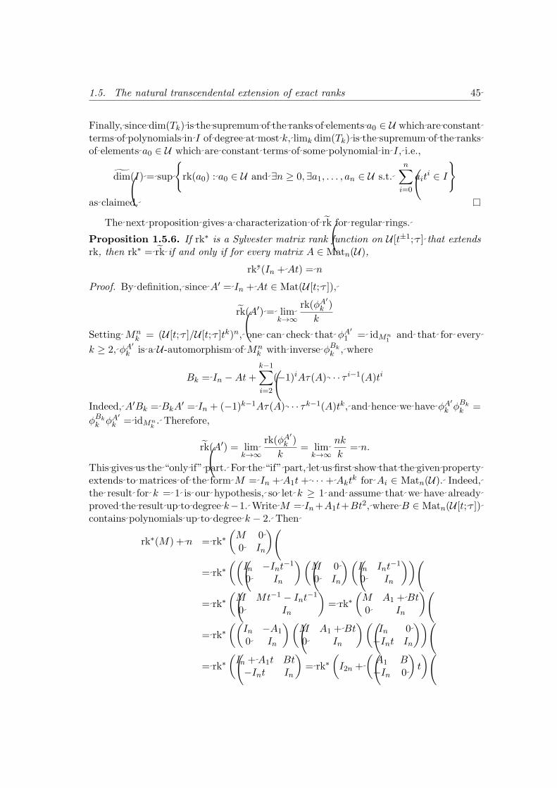
45 1.5. The natural transcendental extension of exact ranks

Finally, since dim(Tk) is the supremum of the ranks of elements a0 ∈ U which are constant terms of polynomials in I of degree at most k, limk dim(Tk) is the supremum of the ranks of elements a0 ∈ U which are constant terms of some polynomial in I, i.e.,( )

nX g i ∈ Idim(I) = sup rk(a0) : a0 ∈ U and ∃n ≥ 0, ∃a1, . . . , an ∈ U s.t. ait i=0

as claimed.

The next proposition gives a characterization of rke for regular rings.

Proposition 1.5.6. If rk∗ is a Sylvester matrix rank function on U [t±1; τ ] that extends erk, then rk∗ = rk if and only if for every matrix A ∈ Matn(U),

rk ∗ (In + At) = n

Proof. By definition, since A0 = In + At ∈ Mat(U [t; τ ]),

rk(φA0 )e krk(A0) = lim

k→∞ k Setting Mn = (U [t; τ ]/U [t; τ ]tk)n , one can check that φA

0 = idMn and that for every k 1 1

Bkk ≥ 2, φA0

is a U -automorphism of Mkn with inverse φ , wherek k k−1X

iBk = In − At + (−1)iAτ(A) · · · τ i−1(A)t i=2

Indeed, A0Bk = BkA0 + (−1)k−1Aτ(A) · · · τk−1(A)tk , and hence we have φA

0 φBk == In k k

Bk φA0

φ = idMn . Therefore,k k k

rk(φA0 )e krk(A0) = lim = lim

nk = n.

k→∞ k k→∞ k This gives us the “only if” part. For the “if” part, let us first show that the given property extends to matrices of the form M = In + A1t + · · · + Akt

k for Ai ∈ Matn(U). Indeed, the result for k = 1 is our hypothesis, so let k ≥ 1 and assume that we have already proved the result up to degree k −1. Write M = In +A1t+Bt2 , where B ∈ Matn(U [t; τ ]) contains polynomials up to degree k − 2. Then � �

rk∗(M) + n = rk∗ M 0 0 In �� �� �� �� In −Int−1 M 0 In Int

−1 = rk∗

0 In 0 In 0 In � � � � M Mt−1 − Int−1 M A1 + Bt

= rk∗ = rk∗ 0 In 0 In �� �� �� �� In −A1 M A1 + Bt In 0

= rk∗ 0 In 0 In −Int In � � � � � �

In + A1t Bt A1 B = rk∗ = rk∗ I2n + t −Int In −In 0

46 Chapter 1. Rank functions

The latter matrix has size 2n × 2n and contains polynomials of degree ≤ k − 1. Hence the inductive hypothesis tells us that its rank is 2n, and we deduce that

rk ∗ (In + A1t + · · · + Aktk) = n

We want to show that rk∗(A) = rk(A) for every matrix A ∈ U [t±1e ; τ ]. Let us show the result for elements p ∈ U [t±1; τ ], and for that purpose consider the left annihilator of p in U [t±1; τ ]

±1Annl(p) = {q ∈ U [t ; τ ] : qp = 0}, which is a left ideal of U [t±1; τ ] satisfying U [t±1; τ ]/ Annl(p) ∼= U [t±1; τ ]p. From the

additivity of gdim we deduce that e grk(p) = 1 − g ; τ ]/U [t±1; τ ]p) = dim(U [t±1dim(U [t±1 ; τ ]p) g= dim(U [t±1 dim(Annl(p)); τ ]/ Annl(p)) = 1 − g Moreover, Proposition 1.5.5 tells us that, for every � > 0, we can find polynomials q1 = b0 + b1t + · · · + bkt

k ∈ U [t±1; τ ]p, q2 = c0 + c1t + · · · + cltl ∈ Annl(p) such that g gdim(U [t±1; τ ]p) ≤ rk(b0) + � and dim(Annl(p)) ≤ rk(c0) + �,

and thus from the previous equalities 1 − rk(c0) − � ≤ e Now, since Urk(p) ≤ rk(b0) + �. is regular, we can find x, y ∈ U such that b0xb0 = b0 and c0yc0 = c0. Hence, on the one

0hand, since q1 = q p for some q0 ∈ U [t±1; τ ],

rk∗(p) ≥ rk∗(q1) ≥ rk∗(b0xq1) = rk∗(b0 + b0xb1t + · · · + b0xbktk)

∗ ∗∗ = rk∗(b0(1 + xb1t + · · · + xbkt

k)) = rk∗(b0) rk(p) − �,= rk(b0) ≥ e where (∗) follows because rk∗(1 + xb1t + · · · + xbkt

k) = 1 as we saw before and using Properties 1.2.2(6.), and (∗∗) holds because rk∗ extends rk. Similarly, on the other hand, since q2p = 0, we see from Properties 1.2.2(5.) that rk∗(p) ≤ 1−rk∗(q2) and consequently

rk∗(p) ≤ 1 − rk∗(q2) ≤ 1 − rk∗(c0yq2) = 1 − rk∗(c0 + c0yc1t + · · · + c0ycltl)

∗ ∗∗ = 1 − rk∗(c0(1 + yc1t + · · · + yclt

l)) = 1 − rk∗(c0) = 1 − rk(c0)

≤ erk(p) + �,

where (∗) and (∗∗) are deduced as in the previous case. Since this is valid for every �, ewe conclude that rk∗(p) = rk(p) for every element p ∈ U [t±1; τ ].

Notice that to prove the result in general it suffices to show that equality holds for m × m matrices, since we can add rows and columns of zeros without changing the rank (Properties 1.2.2(4.)). Moreover, we can restrict our attention to matrices over U [t; τ ], since we can always multiply by the invertible matrix Imt

−k for a suitable k, operation that again leaves the rank unchanged (Properties 1.2.2(2.) & (6.)). Let ϕm be the isomorphism defined in diagram (1.3), and observe that S = Matm(U) is regular� � (Example 1.3.2(c)) and rkm = ϕm

] 1 rk∗ is a rank function on S[t±1; τ ] satisfying, for m every matrix A0 over S, the following:

47 1.5. The natural transcendental extension of exact ranks

1. Since ϕm(A0) = A0 considered as a matrix over S[t±1; τ ], we have � � � � 1 1 rk∗(A0)

rkm(A0) = ϕ] rk ∗ (A0) = rk ∗ (A0) = m m m m � � ∗ rk(A0) 1 = = rk (A0)

n m

1where (∗) holds because rk∗ extends rk. Hence, rkm extends rk. m

2. If A0 is square of size n × n and IS,n denotes the n × n identity matrix over S, � � � � rkm(IS,n + A0t) = ϕ]

1 rk ∗ (IS,n + A0t) =

1rk ∗ (IS,n + A0t)m m m

rk∗(IS,n + A0t) ∗ mn = = = n.

m m

Here, (∗) follows because in the preceding fraction we see IS,n + A0t as a matrix over U [t±1; τ ], and hence IS,n becomes the identity matrix Imn over U . Thus, by hypothesis, rk∗(IS,n + A0t) = nm.

In other words, S, rkm and 1 rk satisfy the hypothesis of the theorem. Thus, as we have m already proved, rkm must coincide with the natural transcendental extension of 1 rk on m

1elements of S[t±1; τ ]. But Lemma 1.4.21 tells us that the natural extension of rk is� � m ] 1 eϕm rk and consequently, for every element A ∈ S[t; τ ], we have m � � � �

1 ] 1rk∗ (ϕm(A)) = ϕm rk∗ (A) = rkm(A)m m � � � � ] 1 e 1 e= ϕm rk (A) = rk (ϕm(A)). m m � �� �

1 1The bijectivity of ϕm gives then the equality rk∗ (B) = rke (B) for every element m m eB ∈ Matm(U [t; τ ]) and hence we have rk∗(B) = rk(B) for every square matrix on U [t; τ ]. This finishes the proof.

Once we introduce and describe in the next chapter the basic properties of the space of Sylvester matrix rank functions on a ring R, we will point out that, when U is regular, the natural transcendental extension of the rank rk is a regular rank function on U [t±1; τ ].

Chapter 2

The space of Sylvester matrix rank functions

In the previous chapter we introduced different notions of rank functions and show how they are related to each other. As discussed during the introduction, the notion of Sylvester matrix (or module) rank function serves both as a classifying tool and as a common language to transcribe and tackle many different problems. This chapter explores the space P(R) of all Sylvester matrix rank functions that can be defined on a given ring R, introduce some of its basic properties and completely describes it for certain families of rings.

The latter part of classification and description comes from [JL20B], and relies heav-ily in the well-known structure of finitely generated modules – or equivalently finitely presented modules, since all the concrete examples we work with are left noetherian (cf. [Rot09, Corollary 3.19]) – for the families considered. This allows us, once we identify potential candidates for extreme points of the space, to actually check that they are extreme and, moreover, that every other rank function in the space is a unique (possibly countably infinite) convex combination of them.

The organization of the chapter is as follows. We introduce in Section 2.1 the space of Sylvester matrix rank functions and the first examples for which we can either describe it completely or relate the spaces associated to different rings. The rest of the sections are each dedicated to describe the space of rank functions on a particular family of rings. We start by studying the space of rank functions on a certain subfamily of left artinian primary rings in Section 2.2. This subfamily appears when dealing with quotients of Dedekind domains and skew Laurent polynomial rings D[t±1; τ ], where D is a division ring and τ an automorphism of D, and therefore allows us to get a partial picture of the space of rank functions for those two families, which are later studied in Section 2.3 and Section 2.5, respectively. In Section 2.4 we discuss the case of simple noetherian rings, which also appears naturally when dealing with Laurent polynomial rings.

49

50 Chapter 2. The space of Sylvester rank functions

2.1 The space P(R) and first examples

Let R be a ring. In this section we introduce and study the basic properties of P(R), the space of Sylvester rank functions on R, and present some basic examples of rings for which we can totally or partially describe P(R). Here, by “describing P(R)” we mean either identifying the extreme points in P(R), so that any other rank function is a convex combination of those, or finding rings S and maps (of sets) P(S) → P(R) that we can show to be injective, surjective or bijective. However, although we shall not be especially concerned about further topological properties of the space, we need some definitions to introduce it properly.

Definition 2.1.1.

- A directed set (I, ≤) consists of a set I together with a reflexive and transitive binary relation ≤ satisfying that, for each i, j ∈ I, there exists k ∈ I such that k ≥ i and k ≥ j.

- If X is a topological space, then a net in X is a map I → X where (I, ≤) is a directed set. If the map sends i 7→ xi, we denote this net as usual by {xi}i∈I .

- We say that a net {xi}i ∈ I in a topological space X converges to x ∈ X if, for every neighborhood U ⊂ X of x, there exists i0 ∈ I such that for every i ≥ i0, xi ∈ U . We say that x is a limit of {xi}i∈I and write xi → x.

Some authors also require the directed set to be antisymmetric, but we do not need this property for our purposes in this chapter.

The point about nets is that they allow us to reformulate some of the most im-portant topological properties that we shall discuss here. The following properties can be found, for the particular case of Hausdorff spaces, in [Con14, Proposition 2.7.7 & Proposition 2.7.8].

Proposition 2.1.2. Let X and Y be topological spaces. Then

1. The space X is Hausdorff if and only if every convergent net in X has a unique limit.

2. A subset C of X is closed if and only if the limits in X of every convergent net {xi}i∈I of points of C lie in C.

3. A map f : X → Y is continuous if and only if for every net {xi}i∈I in X converging to x ∈ X, the net {f(xi)}i∈I in Y converges to f(x).

Moreover, we are going to work essentially with the following two examples of topo-logical spaces, for which the definition of convergence of nets admits a handy character-ization.

51 2.1. The space P(R) and first examples

Example 2.1.3.

1. In R together with the standard topology, a net {xi}i∈I converges to x ∈ R if and only for every � > 0, there exists i0 ∈ I such that for every i ≥ i0, we have |xi − x| < �.

The usual properties of sequences in R extend to nets. For example:

a) If xi → x and yi → y, then xi + yi → x + y and xi − yi → x − y. xi x

b) If xi → x and yi → y with y, yi =6 0 for every i ∈ I, then → . yi y

c) If xi → x, yi → y and xi ≤ yi for every i ∈ I, then x ≤ y.

2. Let X be a set, Y a topological space and M a set of maps f : X → Y . Then M can be seen as a subset of Y X , the cartesian product of |X| copies of Y with the product topology. The induced topology in M under this identification is the so-called pointwise convergence topology.

The name comes from the fact that a net {fi}i∈I in M converges to f ∈ M if and only if for every x ∈ X, the net {fi(x)}i∈I converges to f(x) in Y .

Let for the moment PMat(R) denote the set of Sylvester matrix rank functions on the ring R. As in Example 2.1.3(2.), PMat(R) can be identified with a subset of RMat(R) and hence endowed with the pointwise convergence topology. In particular, given any net {rki}i∈I in PMat(R) and any point in RMat(R), seen as a map f : Mat(R) → R, we have that rki → f in RMat(R) if and only if for every matrix A ∈ Mat(R), rki(A) → f(A) in R.

Therefore, every claim we do about PMat(R) reduces to checking the convergence of the appropriate nets in R. And note also that, as a product of Hausdorff spaces, RMat(R) is again Hausdorff, and hence the limit of a convergent net is unique (Proposition 2.1.2(1.)).

Proposition 2.1.4. PMat(R) is a compact convex subset of RMat(R).

Proof. One can show that if rk1 and rk2 are Sylvester matrix rank functions on R then, for every 0 ≤ λ ≤ 1, the map λ rk1 +(1 − λ) rk2 is again a Sylvester matrix rank function on R, so PMat(R) is a convex set.

Observe now that if rk ∈ PMat(R) and n(A) denotes the number of rows of a given matrix A over R, then 0 ≤ rk(A) ≤ n(A). Thus, we can think of PMat(R) as a subset ofQ

[0, n(A)], which is compact in RMat(R) by Tychonoff’s theorem . Since closed subsets A of compact sets are also compact, we just need to check that PMat(R) is closed, and by Proposition 2.1.2(2.) this is equivalent to show that given a net {rki}i∈I in PMat(R) that converges in RMat(R) to a map f : Mat(R) → R, we have f ∈ PMat(R). Indeed,

(SMat1): Since rki(1) = 1 for every i and rki(1) → f(1) in R, then necessarily f(1) = 1. Similarly f(0) = 0 for every 0 matrix.

52 Chapter 2. The space of Sylvester rank functions

(SMat2): Given matrices A and B that can be multiplied, we have in R that rki(AB) → f(AB) and rki(A) → f(A). Since rki(AB) ≤ rki(A) for every i ∈ I, we have by Example 2.1.3(1.c) that f(AB) ≤ f(A). Similarly f(AB) ≤ f(B).

(SMat3): Let A, B be two matrices over R. We have that rki(A) → f(A), rki(B) → f(B) and rki(A ⊕ B) → f(A ⊕ B) in R. From the first two and Example 2.1.3(1.a) we obtain that the net {rki(A) + rki(B)}i∈I converges to f(A) + f(B). Since rki(A ⊕ B) = rki(A) + rki(B) for every i ∈ I, we have by uniqueness of the limit that f(A ⊕ B) = f(A) + f(B).

(SMat4:) Let A, B, C be matrices of appropriate sizes. As before, we have that rki(A ⊕� � � � � � B) → f(A)+f(B), and rki

A 0

C B → f A

0 C B in R. Since rki

A 0

C B ≥ rki(A⊕B)

for every i ∈ I, again by Example 2.1.3(1.c) we deduce that � � f A

0 C B ≥ f(A) + f(B)

Recall that (SMat2) and (SMat1) are enough to ensure the non-negativity of f , so f is actually a Sylvester matrix rank function and PMat(R) is closed. This finishes the proof.

To describe the space PMat(R), we also need the following terminology.

Definition 2.1.5.

• A Sylvester matrix rank function rk ∈ PMat(R) is called extreme or an extreme point of PMat(R) if it admits no non-trivial expression as a convex combination of two different elements in PMat(R).

• If X and Y are convex sets in the R-vector spaces E1 and E2, respectively, then a map f : X → Y is convex-linear if it preserves finite convex combinations.

Although we will not discuss this in detail, RMat(R) is not only Hausdorff, but a lo-cally convex topological vector space. As a consequence, Krein-Milman theorem states that any compact convex subset K of RMat(R) equals the closure of the convex hull of its extreme points. Moreover, we can allow in such subsets (countably) infinite convex com-binations of points (cf. [Goo91, Proposition A.7]), i.e., if we have an infinite family of points {xi}i∈N in K and non-negative real numbers {λi}i∈N adding up to 1, then the par-P P ntial sums λixi converge to a unique point x in K and we set x = λixi. In the proof i=1 P of [Goo91, Proposition A.7] it is shown that if µi =

Pi λj , then { 1 n λj xj }i∈N isj=1 µi j=1 a sequence in K that converges to x. As a consequence, convex-linear homeomorphisms preserve these infinite convex combinations.

This justifies our attempt to identify the extreme points in PMat(R). Furthermore, in the families of rings we are going to deal with, we show that any Sylvester rank function is uniquely a (possibly infinite) convex combination of those extreme points.

Notice that we can analogously define PMod(R) as the set of all Sylvester module rank functions on R and identify it with a compact convex subset of RFP-Mod , where

53 2.1. The space P(R) and first examples

FP-Mod denotes the set of all finitely presented left R-modules up to R-isomorphism. We show in the next proposition that the bijection in Proposition 1.2.8 defines actually a convex-linear homeomorphism between PMat(R) and PMod(R).

Proposition 2.1.6. The bijection presented in Proposition 1.2.8 defines a convex-linear homeomorphism between PMat(R) and PMod(R). In particular, it preserves the extreme points.

Proof. Recall that we associate to a Sylvester matrix rank function rk the Sylvester module rank function dim defined, on a finitely presented left R-module M ∼= Rm/RnA, by

dim(M) = m − rk(A). To see that the defined map is continuous, we need to check (Proposition 2.1.2(3.)) that for every net {rki}i∈I in PMat(R) converging to a rank rk ∈ PMat(R), the net of associated Sylvester module rank functions {dimi}i∈I in PMod(R) converges to the Sylvester module rank function dim associated to rk. Indeed, by definition we have that for every n × m matrix A over R, {rki(A)}i∈I converges to rk(A) in R, i.e., the net {m − dimi(R

m/RnA)}i∈I converges to m − dim(Rm/RnA). Therefore, by Example 2.1.3(1.a), {dimi(R

m/RnA)}i∈I converges to {dim(Rm/RnA)}. Since this holds for every finitely presented module, this means precisely that {dimi}i∈I converges to dim in PMod(R).

To see that the map is convex-linear, note that given a convex combination rk =P n λi rki of elements in PMat(R), and if dim, dimi denote the associated Sylvester i=1 module rank functions, then for any finitely presented module M ∼= Rm/RnA,

nX dim(M) = m − rk(A) = m − λi rki(A) =

i=1 n nX X

= λi(m − rki(A)) = λi dimi(M), i=1 i=1 P ni.e., dim = i=1 λi dimi.

Analogously, the inverse is also convex-linear and continuous, and thus this yields a convex-linear homeomorphism between the spaces.

For this reason, we do not make in the following any structural distinction between PMat(R) and PMod(R). From now on, we reserve the notation P(R) to refer to PMat(R), and in view of Proposition 2.1.6 we sometimes prove claims about P(R) by showing the corresponding result in PMod(R).

Now that we have properly defined P(R), the next step is to produce Sylvester rank functions. Defining one from scratch is not easy in general, but we have already noticed in Chapter 1 before Definition 1.4.5 that if we have a ring homomorphism ϕ : R → S and a rank function rkS on S, then we can pull back rkS to a rank function rkR = ϕ](rkS ) := rkS ◦ϕ. Therefore, we have the following.

Proposition 2.1.7. Every ring homomorphism ϕ : R → S induces a convex-linear continuous map ϕ] : P(S) → P(R). Moreover, if ϕ is surjective, then ϕ] is injective, and if ϕ is bijective, then ϕ] is a homeomorphism.

54 Chapter 2. The space of Sylvester rank functions

Proof. Let {rk0 i}i∈I be a net in P(S) converging to rk0 ∈ P(S), and let A be any matrix

over R. From the convergence of {rk0 i}i∈I we obtain in particular that

rk0 i(ϕ(A)) −→ rk0(ϕ(A))

But this means precisely that {ϕ](rk0 i)} converges to ϕ](rk0) in P(R), and thus ϕ] isP ncontinuous. Moreover, if we have a convex combination rkS = i=1 λi rki, then by

definition, for every matrix A over R we have

n nX X ϕ](rkS )(A) = rkS(ϕ(A)) = λi rki(ϕ(A)) = λiϕ

](rki)(A), i=1 i=1 P ni.e., ϕ](rkS) = λiϕ

](rki), what proves convex-linearity. i=1 Now, if ϕ is surjective and ϕ](rk0

1) = ϕ](rk0 2), then since any matrix A over S can be

written as ϕ(B) for some matrix B over R, we deduce rk0 1(A) = rk2

0 (A), and therefore rk0 = rk2

0 . And finally, if ϕ is bijective, then ϕ] is a homeomorphism with inverse 1 (ϕ−1)].

Hanfeng Li generalized the result for surjective maps to a broader family of ring homomorphisms, called epic homomorphisms. We give now the definition and we develop further the topic in Chapter 3 and Chapter 4 after introducing epic division and ∗-regular rings.

Definition 2.1.8. A ring homomorphism ϕ : R → S is epic if it is right cancellable, i.e., for any two ring homomorphisms ψ1, ψ2 : S → Q such that ψ1 ◦ ϕ = ψ2 ◦ ϕ, we have ψ1 = ψ2.

For instance, surjective homomorphisms are epic, and for a non-surjective example, the inclusion map R → T −1R, where T −1R stands for the left Ore localization of R with respect to a multiplicative left Ore set T of non-zero-divisors (see Section 3.1), is also epic. This is clear because if two homomorphisms ψ1, ψ2 from T −1R coincide on R, then necessarily one has for every element t−1r ∈ T −1R,

−1 −1ψ1(t r) = ψ1(t)−1ψ1(r) = ψ2(t)

−1ψ2(r) = ψ2(t r).

As a particular example, the embedding Z → Q is epic.

Combining Hanfeng Li’s result [Li20, Theorem 8.1] with Proposition 1.4.7 we obtain the next result.

Proposition 2.1.9. If ϕ : R → S is an epic ring homomorphism, then the induced map ϕ] : P(S) → P(R) is injective. In particular, if S = T −1R is the left Ore localization of R with respect to a multiplicative left Ore set T of non-zero-divisors, then

im ϕ] = {rk ∈ P(R) : rk(t) = 1 for every t ∈ T }.

For us, among the family of rank functions that can be obtained through homomor-phisms, are of particular interest the regular ranks defined in Definition 1.4.5, because we will show later that we can apply to them most of the machinery developed in Section 1.5.

/

� �

55 2.1. The space P(R) and first examples

Definition 2.1.10. For a ring R, we denote by Preg(R) the set of all regular rank functions on R.

As it happens with P(R), Preg(R) enjoys some desirable closure properties. The proof presented here is the one in [Jai19, Proposition 5.9] with minor changes.

Proposition 2.1.11. Preg(R) is a compact convex subset of P(R). In particular it is closed.

Proof. Consider the set of elements of Preg(R) indexed by some index set I. For every i ∈ I there exists a regular ring Ui with a rank function rk0 and a ring homomorphismi

] Qϕi : R → Ui such that rki = ϕ (rk0

i). Construct U = Ui and let πi denote thei i∈I canonical projection πi : U → Ui. For every i ∈ I, we have a commutative diagram

ϕ /R U πi

ϕi � � Ui

where ϕ(r) = (ϕi(r))i∈I . Thus, rk ∗ = π](rki 0 ) defines a rank function on U such thati i

ϕ](rk ∗ i ) = rki. Therefore, every regular rank function on R comes from U . Note that U

is regular because it is a product of regular rings, and hence the convex-linear continuous map ϕ] : P(U) → P(R) satisfies that im ϕ] = Preg(R). Since ϕ] is convex-linear, its image is a convex set, and since ϕ] is continuous and P(U) is compact, then its image is also compact. As a compact set of a Hausdorff space, it is closed.

As a consequence of this proposition, we can prove the result we anticipated at the end of Section 1.5, i.e., the regularity of the transcendental extension when the base ring is regular.

Corollary 2.1.12. Let U be a regular ring, τ an automorphism of U and rk a τ -compatible Sylvester matrix rank function on U with natural transcendental extension e erk. Then rk is regular both as a rank on U [t; τ ] and on U [t±1; τ ].

Proof. As we already observed in Chapter 1, the kth extension rke k of rk on U [t; τ ] is reg-ular since it comes from the regular ring Matn(U) (Example 1.3.2c)). Since Preg(U [t; τ ])

is closed by the previous proposition, rke is also regular as a rank on U [t; τ ]. Now, let (U 0, ϕ, rk0) be a regular envelope of rk (see Remark 1.4.6), so that rk0 is

faithful and rke = ϕ](rk0). Since erk(t) = 1, we deduce that e1 = rk(t) = rk0(ϕ(t)).

Therefore, Lemma 1.3.12 tells us that ϕ(t) (and hence ϕ(tn) for every non-negative integer n) is invertible in U 0 . The universal property of Ore localization (see Proposition 3.1.4 and Example 3.1.7) tells us that ϕ extends uniquely to a ring homomorphism

±1ϕ : U [t ; τ ] → U 0 .

Since ϕ](rk0) is a rank function on U [t±1; τ ] that coincides with rke in U [t; τ ], we deduce ˜ ; τ ], and hence ethat rke = ϕ](rk0) as a rank function on U [t±1 rk is regular on U [t±1; τ ].

56 Chapter 2. The space of Sylvester rank functions

Just as a remark, not every Sylvester matrix rank function is regular, so there are rings R for which the containment Preg(R) ⊆ P(R) is strict.

Example 2.1.13. Not every Sylvester matrix rank function is regular.

Consider the ring R = Z/4Z. Since R is an artinian ring, every finitely generated R-module M has finite length l(M) (in the sense of composition series). In particular, R has finite length 2 and thus, since the length is additive in short exact sequences (cf.

[GW04, Proposition 4.12]), the function dim given by dim(M) = l(M 2) defines a Sylvester

module rank function on R. Observe in particular that if rk is the Sylvester matrix rank 1function associated to dim, then rk(2 + 4Z) = 2 .

We claim that rk is not regular. To see this, first observe that the characteristic of a regular ring cannot be a square. Indeed, let U be a regular ring and assume that

2char(U) = n . Then the element n1 is a non-zero element in the center of U , but by regularity we can find y ∈ U such that n1 = (n1)y(n1) = (n21)y = 0, a contradiction. Therefore, if ϕ : R → U is a ring homomorphism from R to a (non-zero) regular ring, then since char(U) must divide char(R) = 4, we must have char(U) = 2. But then ϕ(2+4Z) = 0 and any rank function coming from U gives 2+4Z value 0. This completes the proof of the claim.

This way of producing rank functions through length of modules also appears in Section 2.2 and Section 2.3.

Besides isomorphic rings, there is another instance of rings for which the spaces of rank functions are homeomorphic: Morita equivalent rings. This is proved in [Goo91, Theorem 17.14] for regular rings, and in full generality in [Li20, Remark 7.1]. Here, we give another proof of this fact for the sake of completeness and in order to state the analog of [Goo91, Proposition 16.20].

Proposition 2.1.14. Let R, S be Morita equivalent rings. Then there exists a homeo-morphism between P(R) and P(S) preserving the extreme points. Moreover, if ι : R → Matn(R) is the diagonal embedding, this homeomorphism is convex-linear and sends

1rk ∈ P(Matn(R)) to the rank function ι](rk) and rk0 ∈ P(R) to the rank function rk0 . n

Proof. Let R-Mod (resp. S-Mod) denote the category of left R-modules (resp. S-modules), and let F : R -Mod → S -Mod, G : S -Mod → R -Mod be the associated equivalence between these categories with FG and GF naturally equivalent to the cor-responding identity functors. Recall that an equivalence of categories preserves direct sums, short exact sequences and finitely presented modules ([Lam99, Section 18A]).

Let dim be a module rank function on S. Since F (R) is a progenerator in S -Mod ([Lam99, Remark 18.10(A)]), S is a direct summand of F (R)n for some positive integer n. Therefore, from (SMod1) and (SMod2) we obtain that dim(F (R)) > 0.

dim(F (N))By the previous remarks, the expression dim0(N) = for an R-module Ndim(F (R)) now defines a Sylvester module rank function on R, so we have a map P(S) → P(R). Similarly, we can define a map P(R) → P(S). Finally, by the natural equivalence, we have FG(M) ∼= M for every S-module M and GF (N) ∼= N for every R-module N . As a consequence, one can check that both maps are mutual inverses.

57 2.1. The space P(R) and first examples

To check the continuity of the given map, let {dimi}i∈I be a net of rank func-tions on P(S) converging to dim ∈ P(S). As we explained before, dim(F (R)) > 0 and dimi(F (R)) > 0 for every i ∈ I. Since by convergence we have that for every finitely presented S-module M , dimi(M) → dim(M) in R, then in particular using Ex-ample 2.1.3(1.b), we obtain that for every finitely presented R-module N ,

dimi(F (N)) dim(F (N))−→ in R,dimi(F (R)) dim(F (R))

what means precisely that the net {dim0 i}i∈I converges to {dim0} in P(R). Thus, the

map P(S) → P(R) is continuous, and similarly P(R) → P(S) is also continuous. Thus, they are homeomorphisms.

Finally, they preserve extreme points. For instance, if we have a convex combina-tion dim = λ dim1 +(1 − λ) dim2 in P(S), where 1 > λ > 0, then we obtain a linear combination

λ dim1(F (R)) (1 − λ) dim2(F (R))dim0 = dim0 dim0

1 + 2dim(F (R)) dim(F (R))

which is convex, since the coefficients are positive and add up to one. For the particular case of S = Matn(R), the equivalences of categories are defined on

objects (cf. [Lam99, Theorem 17.20]) by

F : R -Mod → S -Mod G : S -Mod → R -Mod P n×1P 7→ , Q 7→ E11Q

where E11 is the n×n matrix having 1 in the upper left corner and zeros everywhere else. Observe that E11Q ∼= R1×n ⊗S Q as R-modules and P n×1 ∼= Rn×1 ⊗R P as S-modules. Here, we use the notation R1×n and Rn×1 to make explicit that we are considering rows and columns, respectively, for the module operations to be defined naturally.

Let rk be a Sylvester matrix rank function on S with associated module rank function ∼ 1dim. Since F (R)n = S, we have dim(F (R)) = . Moreover, for any A ∈ Matk×l(R), if n

M = Rl/RkA, there exists an isomorphism of S-modules

n nM M Mn×1 ∼F (M) = = Sl/SkB

i=1 i=1

where B = ι(A). Thus, if rk0 is the Sylvester matrix rank function associated to dim0 as defined before, then

dim(Mn×1)rk0(A) = l − dim0(M) = l − = l − n dim(Mn×1) =

dim(F (R))

= l − dim(Sl/SkB) = rk(B) = ι](rk)(A),

so we conclude that rk0 = ι](rk). Conversely, if rk0 is a Sylvester matrix rank function on R with associated module

rank function dim0 , and we denote by rk and dim the corresponding rank functions on S given by the Morita equivalence, then, from the R-module isomorphisms

G(S) ∼= Rn and R1×n ⊗S Sl/SkB =∼ Rnl/RnkB

58 Chapter 2. The space of Sylvester rank functions

where B ∈ Matk×l(S) is considered on the right as an nk × nl matrix over R, we obtain that

dim0(R1×n ⊗S Sl/SkB)

rk(B) = l − dim(Sl/SkB) = l − = dim0(G(S))

1 1 1 = l − dim0(Rnl/RnkB) = l − (nl − rk0(B)) = rk0(B),

n n n 1from where rk = rk0 . Since this correspondence preserves convex combinations, this n

finishes the proof.

Observe from the previous construction that, in general, the homeomorphism con-structed between the spaces of rank functions of Morita equivalent rings is not convex-linear. A counterexample for convex-linearity is given in [Goo91, Example 17.15].

We finish the section by studying some examples of rings for which we can describe completely the space of Sylvester rank functions. The first one was already mentioned at the beginning of Section 1.3.

Example 2.1.15.

1. On a division ring D, there exists only one rank function, namely, the usual rank rkD. Indeed, since D is regular, every rank function on D is determined by its values on elements, but every non-zero element in D must have rank 1 because it is invertible. Therefore, P(D) = {rkD}.

2. By the previous example and Proposition 2.1.14, for a matrix ring R = Matn(D) over a division ring D, we have P(R) = { 1 rkD}. n

In the following, we relate the space of rank functions on a finite cartesian product of rings with the space on every factor. Together with the previous examples, this gives a complete description of the space of rank functions on a semisimple artinian ring. The example of finite cartesian products of regular rings (and in particular semisimple artinian rings) was already studied in [Goo91, Theorem 16.5 & Corollary 16.6]. The next observation is in order to make precise the statement of the proposition.

Remark 2.1.16. Let R = R1 ×· · ·×Rn and let πi : R → Ri denote the natural projections. We say that the rank rk ∈ P(R) can be uniquely expressed as a convex combination of ranks on Ri if there exist uniquely determined non-negative coefficients λ1, . . . , λnP with λi = 1 and, for every λi > 0, a uniquely determined rki ∈ P(Ri), such thatP ]rk = λiπi (rki).

The assumption that rki exists and it is uniquely determined only for λi > 0 is needed (cf. [Goo91, Theorem 16.5]) to address properly the cases in which some Ri does not admit Sylvester rank functions or that λi = 0 and Ri admits more than one Sylvester rank function (in which case the expression would not be unique).

Proposition 2.1.17. Let R1, R2 be rings. Any Sylvester rank function on R = R1 × R2 is a uniquely determined convex combination of Sylvester rank functions on R1 and R2.

59 2.1. The space P(R) and first examples

In particular, the set of extreme points on P(R) is the disjoint union of the sets of extreme points of P(R1) and P(R2).

Proof. Let πi : R → Ri be the natural projections. Since πi is a surjective ring homo-morphism, the map π] : P(Ri) → P(R) is injective. Consider also the natural additive i maps ιi : Ri → R.

Observe that if A ∈ Matn×m(R), then A = A1 + A2 where A1 = ι1π1(A), A2 = ι2π2(A). Moreover, if In,1 ∈ Matn(R), Im,2 ∈ Matm(R) denote the diagonal matrices whose entries are all equal to (1, 0) and (0, 1), respectively, we have

In,1A1 = A1, In,1A2 = 0, A1Im,2 = 0, A2Im,2 = A2.

Thus, Lemma 1.2.5 tells us that for any rank function rk ∈ P(R), we have

rk(A) = rk(A1) + rk(A2).

In particular, we obtain that 1 = rk((1, 0)) + rk((0, 1)). Now, if rk((1, 0)) = 0, then rk(A1) = rk(In,1A1) ≤ rk(In,1) = n rk((1, 0)) = 0, and if rk((1, 0)) > 0, then the ex-

1pression rk1 = rk ◦ι1 defines a Sylvester matrix rank function on R1. Similarly, rk((1,0)) if rk((0, 1)) = 0 then rk(A2) = 0, and we can define a rank function rk2 on R2 if rk((0, 1)) > 0. One can check that

] ]rk = rk((1, 0))π1(rk1) + rk((0, 1))π2(rk2),

where we understand that rki is considered only when the coefficient is non-zero. More-over, if we had another expression rk = λπ1

] (rk0 1) + (1 − λ)π] (rk2

0 ) for some rk0 i ∈ P(Ri)2

and 0 ≤ λ ≤ 1, then rk((1, 0)) = λ and rk((0, 1)) = 1 − λ. Hence, if λ > 0, then for every matrix B over R1,

rk(ι1(B)) = λ rk1(B) = λ rk0 1(B),

from where rk1 = rk1 0 , and similarly, if 1 − λ > 0, then rk2 = rk2

0 . Thus, the combination is unique.

From the previous expression, one can also deduce that if rk is an extreme point in P(R), then either rk((1, 0)) = 1 and rk1 is an extreme point in P(R1) or rk((0, 1)) = 1 and rk2 is an extreme point in P(R2).

Conversely, if, for instance, rk1 is an extreme point in P(R1), then π] (rk1) is a rank1 ]function on R which takes value 1 on (1, 0). Therefore, if we had π (rk1) = λ rk +(1 −1

λ) rk0 with 1 > λ > 0 and rk 6= rk0 on P(R), then necessarily rk((1, 0)) = rk0((1, 0)) = 1 (and consequently rk((0, 1)) = rk0((0, 1)) = 0). Thus, reasoning as before, we can see

that rk ◦ι1 and rk0 ◦ι1 define rank functions on R1 such that rk = π] (rk ◦ι1) and rk0 = 1 π] (rk0 ◦ι1) (in particular, they are different) and1

rk1 = λ rk ◦ι1 + (1 − λ) rk0 ◦ι1,

which contradicts the fact that rk1 is extreme. This finishes the proof.

Before moving on to the next section, we recall again that all the rings we are going to consider from now on are left noetherian, and hence the words finitely presented and finitely generated are interchangeable for left R-modules. (cf. [Rot09, Corollary 3.19]).

60 Chapter 2. The space of Sylvester rank functions

2.2 Left artinian primary rings

In this section we study the space of Sylvester matrix rank functions on a family of rings which is deeply related to the families in Section 2.3 and Section 2.5, namely, left artinian primary rings. More precisely, we give a description of this space for those left artinian primary rings whose Jacobson radical is generated by a central element. Throughout the section, J(R) denotes the Jacobson radical of the ring R.

Following [Pie82], a ring (Z-algebra) R is local if R/J(R) is a division ring, or equiv-alently, if the set of all non-units in R form a (two-sided) ideal, which is necessarily J(R) (cf. the proof of [Pie82, Proposition 5.2]). A ring R is primary if R/J(R) is simple.

When R is left (or right) artinian, we can reduce the study of the space of rank func-tions on the latter family of rings to the study of local rings through Proposition 2.1.14 and the following result ([Pie82, Proposition 6.5a]).

Proposition 2.2.1. If R is a left artinian primary ring, then there exist a unique s and a unique (up to isomorphism) left artinian local ring S, such that R ∼= Mats(S).

The following example of local artinian ring serves as a motivation for the general treatment.

2.2.1 The case of K[t]/(tn)

If K is a commutative field and n is a positive integer, then the ring R = K[t]/(tn) is an example of local artinian ring. As a consequence of the structure of modules on K[t], every finitely generated R-module can be expressed as a direct sum of the indecomposable R-modules K[t]/(ti) ∼= R/(ti + (tn)), 1 ≤ i ≤ n. Thus, from (SMod2), any Sylvester module rank function on R is determined by its values on these modules, or equivalently, any Sylvester matrix rank function is determined by its values on the elements ti + (tn).

We can define n Sylvester matrix rank functions rk1, . . . , rkn on R through the canon-ical homomorphisms R → EndK (K[t]/(tk)) ∼= Matk(K) with p + (tn) 7→ φp 7→ Ap, wherek φp is the endomorphism given by right multiplication by p + (tk) and Ap is its associated k matrix with respect to the canonical basis in K[t]/(tk) (here, we consider endomorphisms acting on the right, so both are ring homomorphisms). If rkK denotes the usual rank function on K, then the unique rank function on Matk(K) is 1 rkK , and when we pullk it back to R we obtain a regular rank function rkk satisfying (

k−i if i ≤ kkrkk(ti + (tn)) =

0 otherwise

Moreover, any other rank function on R is a convex combination of the above ranks.

Proposition 2.2.2. Let K be a field, n a positive integer and set R = K[t]/(tn). There exist exactly n extreme points in P(R), which are the Sylvester matrix rank functions rk1, . . . , rkn, and any other rank function can be uniquely expressed as a convex combi-nation of the previous ones. As a consequence, P(R) = Preg(R).

61 2.2. Left artinian primary rings

Proof. Let rk be any rank function on R, and consider the system

n nX X rk = ck rkk, ck ≥ 0, ck = 1.

k=1 k=1

As observed previously, any rank function on R is determined by its values on ti + (tn), 1 ≤ i ≤ n − 1. Therefore, for this system to have a solution it is enough to find non-negative ck satysfying

n nX X k − i rk(ti + (tn)) = ck rkk(t

i + (tn)) = ck k

k=1 k=i

for any 0 ≤ i ≤ n − 1, since the equality for i = 0 already encodes that the coefficients add up to 1. Setting bk = rk(tk + (tn)) − rk(tk+1 + (tn)) for 0 ≤ k ≤ n − 1, we obtainP n 1that bk = cj , and so the only possible solution is given by j=k+1 j

ck = k(bk−1 − bk), k = 1, . . . , n − 1, cn = nbn−1 P P n n−1Finally, every ck ≥ 0 by Lemma 1.2.4 and = bk = rk(1 + (tn)) = 1.k=1 ck k=0 Since the solution is unique for every rank, rk1, . . . , rkn are the only rank functions that cannot be expressed as a convex combination of two different ranks and hence they are the extreme points in P(R).

The last assertion follows from the regularity of rkk and the convexity of Preg(R).

While the point of view of matrices is usually easier to understand at first, working with Sylvester module rank functions allows us to use properties that do not have an analog for matrices. In this sense, observe that the associated extreme Sylvester module rank functions dim1, . . . , dimn are determined by (

i if i ≤ kkdimk(R/(ti + (tn))) =

1 otherwise

2.2.2 The general case

Let us now consider any left artinian local ring R. This implies in particular that J(R) is nilpotent (cf. [Pie82, Proposition 4.4] or [GW04, Theorem 4.15]). We show that if we further assume that J(R) is generated by a central element, then essentially the same classification presented above still holds.

Thus, assume that c ∈ Z(R) is such that J(R) = (c), and let n be the smallest npositive integer such that c = 0. Mirroring the previous example we are going to show

that every rank function on R is determined by its values on c, . . . , cn−1 and that the expressions (

i if i ≤ kkdimk(R/(c i)) = 1 otherwise

�

62 Chapter 2. The space of Sylvester rank functions

can be uniquely extended to Sylvester module rank functions dim1, . . . , dimn on R that turn out to be the extreme points in P(R).

Let us first study the structure of modules over this local ring. Since R is local, an element x is either a unit or belongs to J(R). Let x be a non-zero element of J(R) and m the positive integer such that x ∈ J(R)m\J(R)m+1 . Since c ∈ Z(R), then J(R)m = (cm)

mand therefore x = c u for some unit u ∈ R. Now, take A ∈ Matk×l(R) and express every element of A as aij = cmij uij where uij

is a unit (here, mij = 0 if aij is already a unit, and mij = n if aij = 0). Multiplying by invertible matrices we can assume that m11 = min{mij } and a11 = cm11 . Thus, if rij = mij − m11, ⎛ ⎜⎜⎜⎝

1 0 . . . 0 −cr21 u21 1 0

. .. . . . . . .

⎞ ⎟⎟⎟⎠A

⎛ ⎜⎜⎜⎝ 1 −cr12 u12 . . . −cr1l u1l 0 1 0 . .. . . . . . .

⎞ ⎟⎟⎟⎠ =

�� m11c 0 0 B

−crk1 uk1 0 . . . 1 0 0 . . . 1

�for some (k − 1) × (l − 1) matrix B.� D

Using induction we see that A is equivalent to a � matrix of the form D 0 or where D is a diagonal matrix whose entries are either

0

powers ci for some 0 ≤ i ≤ n − 1 or zero. This expression for a matrix implies that every finitely presented left R-module M

can be written in the form Mr M ∼= Rm ⊕ R/(c mi ).

i=1

Moreover, since c ∈ Z(R) and R is local, for each 0 ≤ i ≤ n we have that R/(ci) is an R-bimodule (with the usual operations) of length i. Indeed, under the previous hypothesis one can show that J(R)k−1/J(R)k ∼= R/J(R) for every 1 ≤ k ≤ n, from where it is a simple left R-module, and hence the chain

0 < J(R)i−1/J(R)i < · · · < J(R)/J(R)i < R/J(R)i

is a composition series for R/J(R)i = R/(ci) of length i (in particular, l(RR) = n). In addition, we have R-bimodule isomorphisms (cf. [Rot09, Proposition 2.68])

min{i,j}).R/(c i) ⊗R R/(cj ) =∼ R/(c

Using this fact, one can show that the previous expression for the R-module M is unique (up to reorganization of factors) by tensoring with R/(ci) for every i = 1, . . . , n and comparing lengths.

Proposition 2.2.3. Let R be a left artinian local ring, and assume that there exists an element c ∈ Z(R) with order of nilpotency n such that J(R) = (c). Then any rank

ifunction on R is determined by its values on c for 1 ≤ i ≤ n − 1, and the expressions dim1, . . . , dimn extend uniquely to Sylvester module rank functions on R that are precisely the extreme points in P(R). Any other rank function can be uniquely expressed as a convex combination of the previous ones.

63 2.2. Left artinian primary rings

Proof. The previous expression for a finitely presented left R-module, together with (SMod2), shows that there exists only one way to extend dimk for an arbitrary finitely presented module. More precisely, if we split the decomposition of M as M M

M = Rm ⊕ R/(c mi ) ⊕ R/(c nj ) mi>k nj ≤k

i=1,...,r1 j=1,...,r2 P then dimk(M) = m + r1 +

nj . Thus, observe thatj k

l(R/(ck) ⊗R M)dimk(M) =

k

where l(N) stands for the length of N . Since the tensor commutes with direct sums and it is right exact, and the length of a module is additive on short exact sequences, we deduce that dimk satisfies (SMod1)-(SMod3).

Since any finitely presented module can be written in the above form, we deduce that any Sylvester matrix rank function is determined by its values on c, . . . , cn−1 . Thus, noting that the associated matrix rank functions are the analogues to the extreme ranks on K[t]/(tn), the same argument of Proposition 2.2.2 shows that these are the extreme points in P(R).

Corollary 2.2.4. Let R be a left artinian primary ring, and assume that there exists an element c ∈ Z(R) with order of nilpotency n such that J(R) = (c). Then any rank function on R is determined by its values on ci for 1 ≤ i ≤ n − 1, and the extreme points in P(R) are the Sylvester matrix rank functions rk1, . . . , rkn defined by (

k−i if i ≤ kkrkk(c i) = 0 otherwise

Any other rank function can be uniquely expressed as a convex combination of them.

Proof. By Proposition 2.2.1, there exist a left artinian local ring S, a positive integer s and a ring isomorphism ϕ : R → Mats(S). Notice that, since ϕ is an isomorphism, we have that ϕ(J(R)) = J(Mats(S)) = Mats(J(S)) and it is generated by ϕ(c).

Now, c is a central element, and hence ϕ(c) ∈ Z(Mats(S)), from where necessarily ϕ(c) = Diag (d, . . . , d) for some d ∈ J(S) ∩ Z(S) of order n. In addition, observe thats J(S) = (d).

Thus, in terms of Sylvester matrix rank functions, Proposition 2.2.3 tells us that the extreme points on P(S) are the ranks rk0

1, . . . , rk0 given by n (k−i if i ≤ kkrk0

k(di) =

0 otherwise

1and, by Proposition 2.1.14, 1 rk0 1, . . . , rk0 are the extreme points in P(Mats(S)). There-ns s

fore, since ring isomorphisms preserve the extreme rank functions, we obtain that rk1 =

64 Chapter 2. The space of Sylvester rank functions

ϕ](1 rk0 1), . . . , rkn = ϕ](1 rk0 ) are the extreme points in P(R), and taking into account ns s

that i) =

1 (dirkk(c rkk

0 (Diag , . . . , di)) = rkk 0 (di),s s

rkk(ci) is defined as in the statement.

To finish, we need to check that rank functions on R are determined by their values n−1on c, . . . , c . Given the bijectivity of the maps P(R) → P(Mats(S)) → P(S), if two

rank functions on R coincide on powers of c, their images are rank functions on S that coincide on powers of d, and hence they are equal by Proposition 2.2.3. This finishes the proof.

2.3 Sylvester rank functions on a Dedekind domain

This section is devoted to describing the space of rank functions P(O) defined on a Dedekind domain O which is not a field, since the latter case has already been treated through Section 2.1. We follow [BK00] to recall the basic properties of Dedekind domains, although we also highly recommend [Nar04].

Recall that over a Dedekind domain every non-zero prime ideal is maximal and every non-zero proper ideal can be represented uniquely as a finite product of powers of distinct prime ideals (cf. [BK00, Lemma 5.1.18 & Theorem 5.1.19]). Moreover, every finitely generated O-module M can be expressed as follows ⎛ ⎞

mM M ∼= On ⊕ I ⊕ ⎝ O/m αj ⎠ ,j

j=1

where I is an ideal of O and the mj are (non-necessarily distinct) maximal ideals (cf. [BK00, Theorem 6.3.23], where the uniqueness of such decomposition is also discussed).

The following lemma collects some other basic properties of ideals over Dedekind domains that we shall need for our purposes.

Lemma 2.3.1. Let I be any non-zero ideal over the Dedekind domain O. Then, the following hold.

1. The quotient O/I is an artinian principal ideal ring.

2. I is projective and strongly two-generated, i.e., for every non-zero x ∈ I, there exists y ∈ I such that I = Ox + Oy.

3. For every non-zero ideal J , there exists an O-isomorphism I ⊕ J ∼= O ⊕ IJ .

Proof. The statements correspond, respectively, to [BK00, Proposition 5.1.22], [BK00, Corollary 5.1.23 & Lemma 6.1.1] and [BK00, Lemma 6.1.4].

Observe from Lemma 2.3.1(1) that for every maximal ideal m and positive integer n, nthe quotient ring O/m is a local artinian ring whose unique maximal ideal J(O/mn) =

65 2.3. Sylvester rank functions on a Dedekind domain

nm/mn is (nilpotent and) principal. Let c ∈ m be such that c+m generates m/mn and note that, since different powers of a proper ideal in O are all distinct (for instance, because of the uniqueness of a primary decomposition; see also [BK00, Proposition 5.1.24]), n is precisely the order of nilpotency of this element. Then, Proposition 2.2.3 tells us that there are exactly n extreme Sylvester matrix rank functions rkO/mn ,1, . . . , rkO/mn in,n P(O/mn), which are determined by (

k−i if i ≤ ki krkO/mn,k(c + m n) = 0 otherwise

Hence, we can define Sylvester matrix rank functions on O through the ring homomor-nphisms πm,n : O → O/m . In particular, for any maximal ideal m and positive integer k

we have a rank function rkm,k = π] (rkO/mk,k). We are going to show that the associated m,k Sylvester module rank functions dimm,k satisfy, for every maximal ideal n and positive integer i, ⎧

i if n = m and i ≤ k⎪⎨k dimm,k(O/n i) = 1 if n = m and i > k⎪⎩

0 if n =6 m

Assume first that n 6= m, take any non-zero x ∈ ni\m and let y be as in Lemma 2.3.1(2),� � xi iso that n = Ox + Oy . Then is a presentation matrix for O/n , and therefore y � �

kx + m dimm,k(O/n i) = 1 − rkO/mk ,k k = 0,

y + m

kwhere the last equality follows because, since x ∈/ m, x + mk is invertible in O/m .

Now, for every i < k, let x be a non-zero element of mk , take y such that mi = i+1 kOx + Oy and observe that necessarily y ∈ mi\m . Thus, if c ∈ m is such that c + m

k kgenerates m/m , there exists an element r ∈ O\m, hence a unit in O/m , such that k iy + m = (r + mk)(c + mk), and as before, � � � �

kx + m 0 i dimm,k(O/m i) = 1 − rkO/mk,k k = 1 − rkO/mk,k i k = .

y + m c + m k

i kFinally, if i ≥ k, the generators of m are zero in O/m , and dimm,k(O/mi) = 1.

As a remark here, observe that the local artinian ring (R = O/mn, J = m/mn) is complete (i.e. the natural map R → limi R/J

i is an isomorphism) and separatedT with respect to the J-adic topology (i.e., J i = 0), since J is nilpotent. Thus, if we i further assume that O contains a field k, then k ,→ O → R is injective, and hence Cohen’s theorem on local rings (cf. [Mat80, Theorem 60 & the proof of the subsequent Corollary 1]) tells us that there exists a subfield K of R, with K ∼= R/J ∼= O/m, and a surjective ring homomorphism K[[t]] → R where t maps to the generator of J . In particular, tn is the first power of t in the kernel of the map, and since K[[t]] is a discrete

66 Chapter 2. The space of Sylvester rank functions

valuation ring, this shows that the kernel must be precisely (tn). Hence, we have an isomorphism K[t]/(tn) ∼= R, meaning in particular that in this case all rank functions on

nO/m are regular by Proposition 2.2.2. We can also define the regular rank function rk0 induced by the field of fractions

Q(O). The same arguments show that the associated module rank function dim0 satisfies dim0(O/ni) = 0 for every maximal ideal n and positive integer i.

The structure of finitely generated modules over O and the next proposition show that, in general, any Sylvester module rank function dim on O is determined by its values on the modules considered above.

Proposition 2.3.2. If dim is a Sylvester module rank function on O, then dim(I) = 1 for every non-zero ideal I of O.

Proof. Let I be a non-zero ideal of O. By using Lemma 2.3.1(3) repeatedly, we can seeLkthat for every positive integer k we have I ∼= Ok−1 ⊕ Ik , from wherei=1

k − 1 dim(Ik) k − 1 dim(I) = + ≥ .

k k k Thus, necessarily dim(I) ≥ 1. On the other hand, I is projective and two-generated by Lemma 2.3.1(2), and hence a direct summand of O2 . Since an ideal of O cannot be free of rank 2, its complement C must be non-zero, and the structure of finitely generated modules over O together with the previous argument shows that dim(C) ≥ 1. Since dim(I) + dim(C) = dim(O2) = 2, necessarily dim(I) = 1.

We are going to show that the previous ranks dimm,k and dim0 are the extreme points in P(O) by proving that any rank function dim on O can be uniquely written as X X X

dim = c0 dim0 + cm,k dimm,k, c0, cm,k ≥ 0, c0 + cm,k = 1, m k∈Z+

where m runs through all maximal ideals of O and k through the positive integers. As there can be an uncountable number of maximal ideals in O, for the right hand side sum to make sense we need to show first that there are only countably many non-zero coefficients. For this purpose, note that if such an expression is to hold, then from the definition of dimm,k we obtain that X cm,k

dim(O/m) = . k

k≥1

In particular, if dim(O/m) = 0, then cm,k = 0 for every k. Thus, for our goal it suffices to see that dim(O/m) = 0 for all but countably many maximal ideals.

Notice that the previous equality implies that if dim(O/m) = 0, then dim(O/mk) = 0 for every k, a statement that will follow from Lemma 2.3.4 in our case but may not be true in general for a commutative ring R (From (SMod3) and the surjective

nhomomorphism R/m → R/m we only deduce dim(R/mn) ≥ dim(R/m)). However, we show in the following lemma that the number of pairs (m, k) such that dim(R/mk) > 0 is still countable in this more general setting.

67 2.3. Sylvester rank functions on a Dedekind domain

Lemma 2.3.3. Let dim be a Sylvester module rank function on a commutative ring R. Then, there exist only countably many maximal ideals m such that dim(R/mk) > 0 for some k ≥ 1.

(k)Proof. Fix k ≥ 1 and, for every n ≥ 1, let Sn be the collection of all maximal ideals

of R with dim(R/mk) > 1/n. Suppose that there exists n such that Sn (k)

is infinite, and (k)

take m > n different maximal ideals {mi}mi=1 in Sn . Then, using the Chinese Remainder Theorem and (SMod2),

mX mk k kdim(R/m · · m ) = dim(R/mi ) > > 1.1 · m n i=1

This is a contradiction, since for every ideal I in R, we have dim(R/I) ≤ dim(R) = 1 (k)

by (SMod1) and (SMod3), so Sn must be finite for every n. Therefore, the set S0 = S S (k) k∈Z+ n∈Z+ Sn is countable.

Since the computation of coefficients is going to be very similar to that of Proposition 2.2.2, we need also the following generalization of Lemma 1.2.4.

Lemma 2.3.4. Let dim be a Sylvester module rank function on O and let m be a maximal ideal. If we set bm,0 = dim(O/m) and bm,k = dim(O/mk+1) − dim(O/mk) for k ≥ 1, then bm,k ≥ bm,k+1 for every k ≥ 0.

2 2Proof. For any non-zero x ∈ m , we can find a non-zero element y ∈ m\m such that k+1 k k−1 2m = Ox+Oy by Lemma 2.3.1(2). Observe that we can write then m = mx +m y

0for every k ≥ 1 (with m = O). One can check that the sequences

ϕ0 ψ02O/m −→ O/m −→ O/m → 0,

where ϕ0(r + m) = yr + m2 and ψ0(s + m2) = s + m, and

k+1 ϕk k ψk k+1 → 0,O/m −→ O/m k+2 ⊕O/m −→ O/m

k+2 k+2 k+1where ϕk(r + mk+1) = (yr + m , r + mk) and ψk(s + m , t + mk) = s − yt + m , are all exact. In fact, every ϕk for k ≥ 0 can be shown to be injective, but this is not needed for the proof since the result already follows from (SMod2) and (SMod3).

We are now ready to prove the main result of this section about P(O).

Theorem 2.3.5. The Sylvester module rank functions dim0 and dimm,k, for every max-imal ideal m and k ≥ 1, are the extreme points of P(O), and any other rank function can be uniquely expressed as a (possibly infinite) convex combination of them. In particular, if O contains a field, P(O) = Preg(O).

68 Chapter 2. The space of Sylvester rank functions

Proof. Let dim be any Sylvester module rank function on O. By Lemma 2.3.3, the set S0 of all maximal ideals m such that dim(O/mk) > 0 for some k ≥ 1 is countable, and as we already discussed, only coefficients cm,k corresponding to m ∈ S0 can be non-zero. Thus, we are going to show that there are unique non-negative numbers c0, cm,k summing up to 1 such that X X

dim = c0 dim0 + cm,k dimm,k . m∈S0 k∈Z+

As we deduced from the structure of finitely generated modules over O and Proposi-ition 2.3.2, it suffices to have equality for every module O/n , where n is a maximal ideal

and i ≥ 1. From the definition of dimm,k, its only contribution for these modules is given when m = n. In particular, if n ∈/ S0, the two expressions coincide on O/ni for every i, and if n ∈ S0, the coefficients cn,k should be determined by

i−1 ∞X X dim(O/n i) = cn,k + cn,k

i k

k=1 k=i

Borrowing the notation of Lemma 2.3.4, we obtain that for every i ≥ 0,

∞X 1 bn,i = cn,k.

k k=i+1

Thus the only possible solution is given by the non-negative coefficients (Lemma 2.3.4)

cn,k = k(bn,k−1 − bn,k), k ≥ 1. P P∞We still need to show that k=1 cm,k converges to a number l less than or equalm∈S0 P nto 1, and take c0 = 1 − l. Notice first that bm,k = dim(O/mn+1), and hence thek=0P n sequence of partial sums { bm,k}n is monotonically increasing and bounded above k=0P∞by 1, so the series bm,k is convergent for every m. Moreover, since by (SMod3) andk=0 Lemma 2.3.4 we have bm,k ≥ bm,k+1 ≥ 0 for every k ≥ 0, Abel-Pringsheim theorem (cf. [Har08, §179]) tells us that limk→∞ kbm,k = 0. Therefore, from the inequalities " #

n n n−1 n−1X X X X 0 ≤ cm,k = k(bm,k−1 − bm,k) = bm,k − nbm,n ≤ bm,k ≤ 1,

k=1 k=1 k=0 k=0 P n we obtain, on the one hand, that the sequence of partial sums { k=1 cm,k}n is alsoP∞monotonically increasing and bounded above by 1, and hence that the series k=1 cm,k is also convergent. On the other hand, we also deduce from the previous discussion thatP∞ P∞ P P∞

k=1 cm,k = bm,k. We claim that bm,k converges to a number smallerk=0 m∈S0 k=0 than 1, from where the result is established. Indeed,

∞ ∞X X XX bm,k = sup bm,k,

B⊂S0m∈S0 k=0 m∈B k=0B finite

69 2.4. Krull dimension and simple left noetherian rings

P P and hence, it suffices to prove that for every finite B ⊂ S0, bm,k converges to a m∈B k number below 1. But this follows from the Chinese Remainder Theorem, (SMod2) and (SMod3), since

nXX X n+1) ≤ 1bm,k = dim(O/m n+1) = dim(O/ ∩ m

m∈B m∈B k=0 m∈B

and therefore " # " # ∞ n nXX X X XX bm,k = lim bm,k = lim bm,k ≤ 1,

n→∞ n→∞ m∈B k=0 m∈B k=0 m∈B k=0

where the second equality follows because we are adding a finite number of finite limits. The last assertion of the proposition is a consequence of the previous discussion regarding

nO/m and K[t]/(tn), and that Preg(O) is closed and convex.

2.4 Krull dimension and simple left noetherian rings

In this section we turn to the study of simple left noetherian rings. These rings appear naturally when dealing with skew Laurent polynomial rings since, for instance, for every automorphism of infinite inner order τ (see Section 2.5) of a division ring D, the ring D[t±1; τ ] is simple and noetherian ([GW04, Corollary 1.15 & Theorem 1.17]). Another widely studied subfamily here are the Weyl algebras An(K) over a field of characteristic zero ([GW04, Exercise 2G & Corollary 2.2]).

We show that on a simple left noetherian ring there exists a unique Sylvester rank function, namely, the one induced from its classical left quotient ring (i.e. the left ring of fractions with respect to the set of all non-zero-divisors). This is proved by means of induction on Krull dimension of modules, and we follow the exposition in [GW04, Chapters 15 & 16] to recall the necessary definitions and results.

Let R be a ring and let M be a left R-module. We say that the Krull dimension of M is −1, and we write K. dim(M) = −1, if and only if M is the zero module. Now, given an ordinal α ≥ 0, we write K. dim(M) ≤ α if, for every descending chain M1 ≥ M2 ≥ M3 . . . of submodules of M , we have K. dim(Mi/Mi+1) < α for all but finitely many i. The Krull dimension of a non-zero module M is then α, denoted K. dim(M) = α, if K. dim(M) ≤ α and α is the least such ordinal, and we write l. K. dim(R) to denote the Krull dimension of R as a left R-module.

In addition, if the module M has K. dim(M) = α ≥ 0 and all its proper factor modules have Krull dimension < α, i.e., K. dim(M/N) < α for every non-zero submodule N of M , then M is called α-critical.

Observe, for example, that a non-zero module M has Krull dimension 0 if and only if it is artinian. Notice also that for every division ring D and every automorphism τ of D, the skew Laurent polynomial ring R = D[t±1; τ ] is not left artinian, since we have the infinite descending chain of left ideals

R ⊇ R(1 + t) ⊇ R(1 + t)2 ⊇ . . . ,

70 Chapter 2. The space of Sylvester rank functions

and its Krull dimension is at most 1 (cf. [GW04, Theorem 15.19 & Exercise 15S]. Thus, l. K. dim(D[t±1; τ ]) = 1 (cf. [MR01, Proposition 6.5.4 (iii)] for a more general result).

In general, an ordinal α as in the definition may not exist, so there are modules for which the Krull dimension is not defined. However, this is not the case of noetherian modules over a ring and, in particular, of finitely generated left modules over a left noetherian ring ([GW04, Lemma 15.3]).

The key point to prove the main result is the following lemma due to Stafford (cf. [Sta76, Lemma 1.4]; see also [Len00, Lemma in page 138]). He originally considered modules M with finite Krull dimension, since it turns out to give an upper bound for the minimal number of generators of M , but the same result holds without this assumption. We add a proof here for the sake of completeness, just following the lines of [GW04, Theorem 16.7]. For this purpose, recall that an R-module M is faithful if annR(M) = 0, fully faithful if all its non-zero submodules are faithful, and completely faithful if all its non-zero factor modules are fully faithful.

Lemma 2.4.1. Let R be a left noetherian ring and M a non-zero finitely generated completely faithful left R-module. If K. dim(M) < l. K. dim(R), then there exists a cyclic submodule N of M such that K. dim(M/N) < K. dim(M).

Proof. Assume K. dim(M) = α ≥ 0, and let Jα(M) denote the intersection of the kernels of all homomorphisms from M to α-critical modules (i.e., the Krull radical of M). Then, Jα(M) is a proper submodule of M , the factor module M/Jα(M) has Krull dimension α ([GW04, Proposition 15.11]) and hence it is fully faithful by hypothesis. Thus, [GW04, Lemma 16.4] tells us that there exists m ∈ M such that (Rm + Jα(M))/Jα(M) is an essential submodule of M/Jα(M), and this is the case if and only if K. dim(M/Rm) < α by [GW04, Corollary 15.12].

With this, we can now state the main result.

Proposition 2.4.2. If R is a left noetherian simple ring, then P(R) = {dimQl(R)}, where Ql(R) is the classical left quotient ring of R.

Proof. Observe that since R is left noetherian and simple, the classical left quotient ring of R exists and it is simple artinian (cf. [GW04, Corollary 6.19]). Therefore, Ql(R) is (isomorphic to) a matrix ring over a division ring and hence it has only one rank function, that we denote by dimQl(R).

Notice also that the simplicity of R implies that every non-zero left R-module is faithful. In particular, every non-zero finitely generated left R-module is completely faithful. We are going to use Lemma 2.4.1 and transfinite induction to show that for every Sylvester module rank function dim on R and for every finitely generated M with K. dim(M) < l. K. dim(R) (equivalently, for every finitely generated torsion module, see [GW04, Proposition 15.7]), we have dim(M) = 0.

The case K. dim(M) = −1 follows from (SMod1) and, at every inductive step, if M is finitely generated with K. dim(M) < l. K. dim(R), then so is Mk , the direct sum of k copies of M , for every positive integer k (cf. [GW04, Corollary 15.2]). Therefore, Lemma 2.4.1 tells us that Mk contains a cyclic submodule N such that K. dim(Mk/N) <

��

71 2.5. Skew Laurent polynomials over division rings

K. dim(Mk). By induction hypothesis, dim(Mk/N) = 0 and, since N is cyclic, (SMod3) tells us that dim(N) ≤ 1. Thus, from the short exact sequence 0 → N → Mk → Mk/N → 0, we obtain that dim(M) ≤ 1 for every k in view of (SMod2) and (SMod3). k Therefore, the previous claim follows.

Taking into account that, for every non-zero-divisor x ∈ R, right multiplication by x defines an injective endomorphism of left R-modules R → R, we obtain K. dim(R/Rx) < l. K. dim(R) by [GW04, Lemma 15.6]. Thus, if rk denotes the Sylvester matrix rank function associated to dim, we deduce

rk(x) = 1 − dim(R/Rx) = 1

Therefore, by Proposition 2.1.9, rk can be extended to Ql(R), and by uniqueness of the rank in Ql(R), dim must be the rank induced by dimQl(R).

We finish the section with another consequence of Lemma 2.4.1 that will prove useful later (see also [Len00, Eisenbud-Robson result, page 131] for the latter part in the simple noetherian case, which can actually be adapted to this situation). We say that a ring R is almost simple (as introduced in [Jai99]) if every non-zero two-sided ideal of R contains a non-zero element from its center Z(R). We shall say that a left R-module M is Z(R)-torsionfree if for all non-zero c ∈ Z(R) and for all non-zero m ∈ M , we have cm 6= 0 (Note that in the language of [GW04, page 81] this would be called a Z(R)\{0}-torsionfree module).

Proposition 2.4.3. Let R be a left noetherian almost simple ring with center Z(R), and let dim be a Sylvester module rank function on R. If l. K. dim(R) ≥ 1 and M is a Z(R)-torsionfree left R-module of finite length, then dim(M) = 0.

Proof. Notice first that every non-zero Z(R)-torsionfree module M with finite length is completely faithful. Indeed, assume that there exists N M such that M/N is not fully faithful, and let L be a submodule of M with N L and L/N not faithful. Then annR(L/N) is a non-zero two-sided ideal of R, and hence it contains a non-zero element c ∈ Z(R). Thus, cL ⊆ N ( L. However, since L ≤ M , we have that L is Z(R)-torsionfree of finite length and therefore the map ϕc : L → L defined by left multiplication by c, which is an R-homomorphism because c ∈ Z(R), is injective. By additivity of length (cf. [GW04, Proposition 4.12]), it must also be surjective, from where L = im ϕc = cL, a contradiction.

Observe now that for every k ≥ 1, Mk is also Z(R)-torsionfree and has finite length. In particular, K. dim(Mk) = 0 and we can apply Lemma 2.4.1 to deduce that Mk is cyclic.

1By (SMod3), dim(Mk) ≤ 1 for every k, and hence (SMod2) implies that dim(M) ≤ k for every k, from where dim(M) = 0.

2.5 Skew Laurent polynomials over division rings

This section focuses on describing the space of rank functions associated to a skew Lau-rent polynomial ring D[t±1; τ ], where D is a division ring and τ is an automorphism of D.

72 Chapter 2. The space of Sylvester rank functions

Unless otherwise specified, throughout this section R denotes a skew Laurent polynomial ring of this form.

The main result of the section describes the extreme rank functions on R and shows that every rank function on R is the unique extension of a rank function on its center Z(R) (cf. Question 1). We also notice at the end of the section that the same theory developed for this ring can be applied to the usual polynomial ring D[t] and, more generally, to the polynomial rings with coefficients on a simple artinian ring.

In order to prove this, we need to recall the structure of two-sided ideals and the center of R, and we start with the description of the latter in the following lemma (cf. [BK00, Lemma 3.2.14]). Recall that the inner order of an automorphism τ is the smallest positive integer m such that τm is an inner automorphism, and we say that τ has infinite inner order if no positive power of τ is inner. Over a division ring D, infinite inner order of the automorphim τ of D is equivalent to the simplicity of D[t±1; τ ] (cf. [GW04, Theorem 1.17]).

Lemma 2.5.1. Denote K = Z(D), and let Kτ denote the subfield of K formed by the elements of K fixed by the automorphism τ of D. Then,

(i) If τ has infinite inner order, then Z(R) = Kτ .

(ii) If τ has inner order m, say τm(d) = a−1da for some a ∈ D, and k is the smallest positive integer for which there exists a non-zero b ∈ K such that τ (bak) = bak ,

tkm)±1].then Z(R) = Kτ [(bak P Proof. Take an element p ∈ Z(R), p = ait

i . Since it must commute with every element d ∈ D, we obtain that dai = aiτ

i(d) for every i, and since p commutes with t, we have ai = τ(ai). Thus, if τ has infinite inner order, we obtain from the first condition that ai = 0 for every i =6 0 and a0 ∈ K, and from the second that actually a0 ∈ Kτ . Thus, p ∈ Kτ . Since clearly Kτ lies in the center, we obtain (i).

If, on the contrary, τ has inner order m, then we obtain from the first condition that ai = 0 for every i not dividing m, and that τmj is given by conjugation by amj whenever it is non-zero. But τmj is also given by conjugation by aj , so for every d,

−1 a −j daj = amj damj .

We deduce that amj a−j ∈ K, i.e., there exists a non-zero cj ∈ K such that amj = cj a

j . From the second condition we obtain now that a0 = c0 ∈ Kτ , and for every j =6 0,

jτ(cj aj ) = cj a , from where the choice of k implies that k ≤ |j|. We claim that k divides

|j| and cj b−j/k ∈ Kτ . Indeed, let sgn(j) denote the sign of j (i.e., sgn(j) = 1 if j is

sgn(j) |j| j )sgn(j)positive and −1 if it is negative), so that c a = (cj a , and notice that ifj sgn(j)|j| = kn + l for some n ≥ 1 and 0 ≤ l < k, then c b−n ∈ K andj

sgn(j) sgn(j) sgn(j) sgn(j) lb−nτ(c b−n a l) = τ(c a|j|(bak)−n) = c a|j|(bak)−n = c a .j j j j

sgn(j)The minimality of k implies l = 0 and thus cj b−n ∈ Kτ , so cj b

−j/k ∈ Kτ .

73 2.5. Skew Laurent polynomials over division rings

P krtmkr As a consequence, there exists zr ∈ Kτ such that p = zrb

ra . Since r tmk)r br rktrmk tmk)r(bak = a and, for every d ∈ D, d(bak = (baktmk)rd, p can be seen

as a Laurent polynomial in the commuting variable baktmk with coefficients in Kτ . Con-versely, every such polynomial p belongs to the center. Thus, Z(R) is the ordinary Laurent polynomial ring Kτ [(baktmk)±1] and we have proved (ii).

Note that there always exists an element b as in the hypothesis. Indeed, when τ has finite inner order m we have that R is not simple and, as we would have also deduced from Lemma 2.5.3(1.), Z(R)∩D[t; τ ] * D (For a concrete example, see [GW04, Exercise 1U]). Now, for every p ∈ (Z(R)∩D[t; τ ])\D, we saw in the proof that every non-zero coefficient corresponding to positive degree mj is of the form cj a

j , cj ∈ K and τ (cj aj ) = cj aj , as

desired. More than its precise description, it is important to observe that if R is non-simple,

the center of R is an ordinary Laurent polynomial ring over a field, and hence every result in this section also applies to the center. When R is simple, the center is a field and we obtain the following from Proposition 2.4.2.

Corollary 2.5.2. If τ has infinite inner order, the only Sylvester rank function on R is the one coming from its Ore division ring, and extends the unique Sylvester rank function on Z(R).

The last assertion of the corollary follows since in Z(R), a field, there exists a unique rank function, which is then necessarily the restriction of the unique rank function in R.

For the rest of the section, assume that τ has finite inner order and let us denote S = Z(R) ∩ D[t; τ ], which is an ordinary polynomial ring over a field by Lemma 2.5.1. In the following lemma we relate two-sided ideals of R and elements of S. Recall that a non-constant p ∈ S is irreducible if it cannot be expressed as a product p = rq for some non-constant r, q ∈ S. Recall also that p, q ∈ S are said to be associates if there exist

0r, r0 ∈ S such that p = rq, q = r p. A comparison of degrees shows that this is the case if and only if p = dq for some unit d ∈ Z(R) ∩ D.

Lemma 2.5.3. The following hold:

(1.) Let I be a non-zero proper two-sided ideal of R. Then, there exists a non-constant polynomial p ∈ S with non-zero constant term such that p generates I and which is irreducible in S if and only if I is maximal.

(2.) There exists a bijective correspondence between maximal two-sided ideals in R and irreducibles in S with non-zero constant term up to association. This defines a bijective correspondence between maximal two-sided ideals of R and maximal ideals of Z(R) sending m to mZ = m ∩ Z(R).

(3.) If m1, . . . , mn are different maximal two-sided ideals in R, then for all positive T ki k1 knintegers k1, . . . , kn, we have i m = m . . . m .i 1 n T (4.) Every non-zero proper two-sided ideal I in R is of the form i m ki for some maximali

two-sided ideals m1, . . . , mn and positive integers k1, . . . , kn.

74 Chapter 2. The space of Sylvester rank functions

Proof. (1.) Let p be a non-zero element of I ∩D[t; τ ] of smallest degree, and note that p is non-constant because I is proper. In addition, p has non-zero constant term because otherwise pt−1 ∈ I ∩D[t; τ ] would be a polynomial of lower degree. Since D is a division ring, we can take 1 as the constant term. Now, p commutes with t because p and tpt−1

have constant term 1 and (p − tpt−1)t−1 ∈ I ∩ D[t; τ ] has lower degree than p, and thus it must be zero. Similarly, p commutes with every element of D, and we deduce that p ∈ Z(R), i.e., p ∈ S.

Since D is a division ring and τ is an automorphism, we can divide polynomials in D[t; τ ] (cf. [BK00, 3.2.6]) and hence, given any other p0 ∈ I and an integer k such that tk 0p0 ∈ I ∩D[t; τ ] we have tkp = qp + r for some q, r ∈ D[t; τ ] with deg(r) < deg(p). Since

0r ∈ I ∩ D[t; τ ], r must be zero, and thus p = (t−kq)p. Therefore, I = Rp as claimed. Assume now that I is not maximal and let J be a proper two-sided ideal properly

containing I. Then J = Rq for some q ∈ S as above, and hence p = rq for some r ∈ R. Since p, q have non-zero constant term, a comparison of degrees shows that r ∈ D[t; τ ] and 0 < deg(r), deg(q) < deg(p). In addition, for every q0 ∈ R, we have

0 0 0 0 0 q rq = q p = pq = rqq = rq q

from where q0r = rq0 since R is a domain. Thus, r ∈ S and p = rq is a product of non-constant polynomials in S of lower degree and therefore p is not irreducible in S.

Conversely, assume that p is not irreducible in S, and let r, q ∈ S be non-constant with p = rq. Note in particular that 0 < deg(r), deg(q) < deg(p), and that q must have non-zero constant term. Therefore J = Rq is a proper two-sided ideal of R with I ( J (since deg(q) < deg(p) and both have non-zero constant term) and hence I is not maximal.

(2.) By (1.), every maximal ideal m is generated by an irreducible element p ∈ S with non-zero constant term. Conversely, if q ∈ S is irreducible with non-zero constant term we can check as in the final step of (1.) that Rq is a maximal two-sided ideal of R.

Let m1, m2 be maximal two-sided ideals in R, and assume mi = Rpi for irreducible p1, p2 ∈ S with non-zero constant term. If m1 = m2, then p2 = r1p1 and p1 = r2p2 for some r1, r2 ∈ R. Reasoning as above we can show that ri ∈ S, and since R is a domain, we obtain from p2 = r1r2p2 that they are units of D. Thus p1 and p2 are associates in S. Conversely, distinct maximals have non-associate generators, and the correspondence is bijective.

tkm Now, let Z(R) = Kτ [s±1] with s = bak as in Lemma 2.5.1. Then S = Kτ [s] and, since Z(R) is again a Laurent polynomial ring over a field, the same argument above shows that the correspondence between maximal ideals of Z(R) and irreducibles in S with non-zero constant term (up to association) is bijective. Therefore, we have a bijection that sends the maximal two-sided ideal m = Rp to the maximal ideal mZ = Z(R)p. Moreover, mZ = m ∩ Z(R), because if x = rp ∈ m ∩ Z(R) for some r ∈ R, then the same argument in (1.) shows that r ∈ Z(R), and hence x ∈ mZ . The other containment is clear.

(3.) Assume that mi = Rpi for pi ∈ S irreducible with non-zero constant term. On k1 kn kn kithe one hand, note that m . . . m = Rpk1 . . . p . On the other hand, let1 n 1 n ⊆ ∩imi

75

1

2.5. Skew Laurent polynomials over division rings

ki k1q ∈ S with non-zero constant term be such that ∩im = Rq. = i In particular, q = r1p · · · = rnp

kn for some r1, . . . , rn ∈ R and as above we can deduce that ri ∈ S. But Sn is an ordinary polynomial ring over a field, hence a unique factorization domain, and

k1 knp1, . . . , pn are non-associate irreducibles in S. Thus, necessarily p1 . . . pn divides q in ki k1 knS, and therefore we also have ∩imi ⊆ m1 . . . m .n

k1 kn(4.) If I = Rp for some p ∈ S with non-zero constant term and p = up . . . p in S1 n with pi ∈ S non-associate irreducibles and u a unit, then pi has non-zero constant term and we deduce from the proof of (3.) that I = ∩im ki where mi = Rpi.i

Before getting to the description of P(R), we obtain a partial picture by analysing nquotient rings R/m for maximal two-sided ideals m. Observe that if I is a non-zero

proper two-sided ideal generated by a central element q ∈ S with non-zero constant term, then R/I is a left D-module with dimD(R/I) = deg(q) and with a natural D-basis {1 + I, . . . , tdeg(q)−1 + I}.

Proposition 2.5.4. For any maximal two-sided ideal m of R and positive integer n, there are exactly n extreme points on P(R/mn). Moreover, P(R/mn) = Preg(R/mn) and the natural embedding ϕn : Z(R)/(mn ∩Z(R)) → R/mn gives a bijection ϕn] : P(R/mn) → P(Z(R)/(mn ∩ Z(R))).

Proof. By Lemma 2.5.3(1.), there exists p ∈ S with non-zero constant term and irre-ducible over S such that m = Rp. In particular, this implies that mZ = m∩Z(R) = Z(R)p is also a maximal ideal of Z(R) by Lemma 2.5.3(2.).

For n = 1, R/m is simple because m is maximal. It is also left (and hence right; see [GW04, Corollary 4.18]) artinian because every descending chain of left ideals of R/m is also a descending chain of left D-modules, and since R/m is finite D-dimensional, it must stabilize. Thus, R/m is isomorphic to a matrix ring over a division ring, and hence it has only one rank function rk. In this case Z(R)/mZ is a field and hence its unique

]rank function must then coincide with ϕ1(rk). nFor n ≥ 2, R/m is a left artinian ring by the previous argument with a unique

n nmaximal two-sided ideal m/m = (p + mn). Since p + m is central nilpotent (with order of nilpotency n), we have p +mn ⊆ J(R/mn) and hence by maximality J(R/mn) = (p+mn). Therefore, J(R/mn) is generated by a central element and (R/mn)/J(R/mn) = (R/mn)/(m/mn) =∼ R/m is simple.

Summing up, R/mn is a left artinian primary ring whose Jacobson radical is generated by a central element of order of nilpotency n. By Corollary 2.2.4, every rank function

n i non R/m is determined by its values on p + m for 1 ≤ i ≤ n − 1, and there are exactly n extreme rank functions rkR/mn,j on P(R/mn), defined by (

j−i if i ≤ jirkR/mn,j (p + m n) = j 0 otherwise.

n nNow, fix 1 ≤ j ≤ n. Any element q + m ∈ R/m gives rise to an endomorphism of the left D-module R/mj given by right multiplication by q. If deg(p) = l, then R/mj has

76 Chapter 2. The space of Sylvester rank functions

jD-dimension jl as noticed before and hence, fixing any basis of R/m , we have a ring nhomomorphism ψ : R/m → EndD(R/mj ) =∼ Matjl(D) (recall that the endomorphisms

nact on the right). Therefore, we can define rank functions rk0 = ψ]( 1 rkD) on R/mR/mn,j jl and, although the latter isomorphism depends on the choice of the basis, the rank does not, since it is invariant under multiplication by invertible matrices. In particular, the image of pi + mn with respect to the basis

j l−1 j j l−1 j j−1 j l−1 j−1{1 + m , . . . , t + m , p + m , . . . , t p + m , . . . , p + m , . . . , t p + mj }

is the jl × jl matrix of normalized rank j− ji

� � 0 I(j−i)l 0 0

when i ≤ j, and the zero matrix otherwise. Therefore, necessarily rkR/mn,j = rk0 R/mn,j

and the extreme ranks are regular. Since Preg(R/mn) is convex, every rank is regular. nFinally, since Z(R) is also a Laurent polynomial ring and mZ = mn ∩ Z(R), we have

nthe same description of P(Z(R)/m ), i.e., every rank function is determined by its values Z i non p +m and there are n extreme points rkZ(R)/mn ,j defined as above on these elements. Z Z

i n i n ]Since ϕn sends p + m to p + m , the ranks ϕn(rkR/mn,j ) and rkZ(R)/mn ,j give them theZ Z same value, and hence they are equal. Since the extreme points go to the extreme points

]and ϕn preserves convex combinations, this finishes the proof.

As a consequence of the previous classification, we deduce the following result.

Corollary 2.5.5. Let I be a non-zero proper two-sided ideal of R. If I = Rp with p ∈ S k1 knwith non-zero constant term and p = up1 . . . pn is a factorization of p into non-associate

jirreducibles of S, then every rank function on R/I is determined by its values on pi + I for i = 1, . . . , n, j = 1, . . . , ki.

Proof. We noticed during the proof of Proposition 2.5.4 that the statement holds when I is a power of a maximal ideal. For the general case, as in the proof of Lemma 2.5.3(4.), I = ∩im ki , where mi = Rpi are different maximal ideals of R. Since powers of differ-i ent maximal two-sided ideals are comaximal, we have a ring isomorphism ϕ : R/I →Q ki i R/m by the Chinese Remainder Theorem. Take a rank function rk ∈ P(R/I), andi Q kiassume that rk = ϕ](rk0) for rk0 ∈ P( R/m ).i iQ ki kiIn view of Proposition 2.1.17, if πi : R/m → R/m denotes the i-th projection, i i i

rk0 can be uniquely written as a convex combination

rk0 = λ1π] (rk1) + · · · + λnπ

] (rkn)1 n

ki ks ksfor some rki ∈ P(R/m ). Now, by comaximality, pi + m is a unit in R/m for every i s s js 6= i, and therefore rks(pi + mks ) = 1 for every s 6= i and every j ≥ 1. Thus, s

j j ks j kirk(pi + I) = rk0((pi + m )s) = λi rki(pi + m ) + (1 − λi).s i

77

i

2.5. Skew Laurent polynomials over division rings

As a consequence, if we know the values of rk on the previous elements, then on the one hand we can compute the coefficients λi via

ki ki kirk(p + I) = λi rki(p + m ) + (1 − λi) = 1 − λii i i

j kiand, on the other hand, for every λi > 0, we can compute the values of rki on pi + m for j = 1, . . . , ki − 1. As in the proof of Proposition 2.5.4, this information determines rki uniquely, so we have completely determined rk.

We have now enough information to determine P(R) when τ has finite inner order. nLet m be any maximal two-sided ideal of R. The ring homomorphisms πm,n : R → R/m

for n ≥ 1 allow us to define rank functions on R. In particular, if m = Rp for some irreducible p ∈ S with non-zero constant term, then for any positive integer k we have a rank function rkm,k, which in the notation of Proposition 2.5.4 can be written as

π] (rkR/mk,k), satisfying m,k (k−i if i ≤ kkrkm,k(p i) = 0 otherwise.

Moreover, if q ∈ S is irreducible with non-zero constant term and not associated to p, then n = Rq defines a different maximal two-sided ideal by Lemma 2.5.3(2.), and hence

nn+m = R for every n ≥ 1. Thus, q becomes a unit in every quotient R/mn and therefore rkm,k(q

i) = 1. In terms of the associated Sylvester module rank functions dimm,k we have then for a two-sided maximal ideal n,

dimm,k(R/n i) =

⎧⎪⎨ ⎪⎩ i k if n = m and i ≤ k 1 if n = m and i > k 0 if n 6= m

We can also define the rank function rk0 coming from its Ore quotient ring, whose associated module rank function dim0 satisfies dim0(R/n

i) = 0 for every maximal two-sided ideal n and i ≥ 1. We are going to prove that, in analogy to the case of Dedekind domains, these are the extreme rank functions on R. For this, we note first the following analog of Lemma 2.3.3, which is proved similarly invoking Lemma 2.5.3(3.).

Lemma 2.5.6. Let dim be a Sylvester module rank function on R = D[t±1; τ ]. There exist only countably many maximal two-sided ideals m of R such that dim(R/mk) > 0 for some k ≥ 1.

Secondly, from Lemma 2.5.3(1.) we know that R is almost simple, and we observed in Section 2.4 that l. K. dim(R) = 1. Hence, we can use Proposition 2.4.3 to deduce in the next proposition that the rank of a finite D-dimensional R-module M is determined by its Z(R)-torsion submodule

tZ(R)(M) = {m ∈ M : cm = 0 for some non-zero c ∈ Z(R)}.

78 Chapter 2. The space of Sylvester rank functions

Note that in the language of [GW04, page 83] this would be called Z(R)\{0}-torsion submodule, and it is actually a submodule because R is a domain and Z(R) is commu-tative.

Proposition 2.5.7. If M is a finitely generated R-module with dimD(M) < ∞, then, for any Sylvester module rank function dim ∈ P(R), we have dim(M) = dim(tZ(R)(M)).

Proof. Denote N = tZ(R)(M) and let dim be a Sylvester module rank function on R. If N = 0, then M is Z(R)-torsionfree of finite length (since it is finite D-dimensional) and hence dim(M) = 0 = dim(N) by Proposition 2.4.3. Assume now that N is non-zero. Since R is noetherian, N is also finitely generated, say, by {m1, . . . ,mn}. For every k, we can take a non-zero pmk ∈ Z(R) ∩ D[t; τ ] with non-zero constant term that annihilatesQ mk and observe that, if p = , then N = {m ∈ M : pm = 0}. Since p ∈ Z(R), pMk pmk

is a submodule of M , and we claim that M = N ⊕ pM . 2Indeed, their intersection N ∩ pM is trivial, because if pm ∈ N , then p m = 0, from

where m ∈ N (by definition, since 0 6= p2 ∈ Z(R)), and therefore pm = 0. Now, from the exact sequence (of D-modules) 0 → N → M → pM → 0, where the homomorphism M → pM is given by left multiplication by p,, we obtain that dimD(M) = dimD(N) + dimD(pM), and hence, since from the second isomorphism theorem and additivity of dimD,

dimD(N + pM) + dimD(N ∩ pM) = dimD(N) + dimD(pM) = dimD(M),

we deduce that M = N ⊕ pM . Since pM is Z(R)-torsionfree of finite length, Proposi-tion 2.4.3 gives that dim(pM) = 0, and therefore dim(M) = dim(N) by (SMod2).

Theorem 2.5.8. The extreme points on P(R) are precisely the rank functions dimm,k and dim0 defined above, and any other rank function can be uniquely expressed as a (possibly infinite) convex combination of them. Thus, P(R) = Preg(R). Moreover, the inclusion map ι : Z(R) → R gives a bijection ι] : P(R) → P(Z(R)).

Proof. Consider a Sylvester module rank function dim on R. Let S0 be the set of two-sided maximal ideals m for which there exists k with dim(R/mk) > 0, which is countable by Lemma 2.5.6. We are going to show that there exist non-negative real numbers c0, cm,k satisfying X X X X

dim = c0 dim0 + cm,k dimm,k and c0 + cm,k = 1. m∈S0 k∈Z+ m∈S0 k∈Z+

Set bm,0 = dim(R/m) and bm,k = dim(R/mk+1) − dim(R/mk) for every k ≥ 1. Since km = Rp for some irreducible p ∈ S = Z(R) ∩D[t; τ ] and m = Rpk , Lemma 1.2.4 implies

that bm,k ≥ bm,k+1 for every k ≥ 0. Thus, if we impose equality of both expressions on the modules R/ni for maximal two-sided ideals n and i ≥ 1, we can reason as in Theorem 2.3.5 to show that the only possible solution is given by the non-negative coefficients

cm,k = k(bm,k−1 − bm,k), k ≥ 1

79 2.5. Skew Laurent polynomials over division rings

P P and that c0 = 1 − k∈Z+ cm,k is well-defined. Nevertheless, we do not know in m∈S0 principle that a rank function on R is already determined by its values on those modules, so we still need to check that this is sufficient to claim equality. Define

X X dim0 := c0 dim0 + cm,k dimm,k

m∈S0 k∈Z+

We have just seen that dim0 is a Sylvester module rank function on R that coincides with dim on the modules R/nk for every maximal two-sided ideal n and k ≥ 1.

Take now any non-zero proper two-sided ideal I such that dI = dim(R/I) > 0, and notice that dim0(R/I) = dI (by using Lemma 2.5.3(4.), the Chinese Remainder Theorem and that dim and dim0 coincide on quotients by powers of maximal ideals). Now, 1 1dim and dim0 define Sylvester module rank functions on R/I. Indeed, any finitelydI dI

presented R/I-module is a finitely generated R-module with the natural operation, and hence finitely presented because R is noetherian. Thus, they satisfy (SMod1)-(SMod3) because dim and dim0 do. But if I = Rq for q ∈ S with non-zero constant term and

k1 knq = uq . . . q for some non-associate irreducibles qi ∈ S and a unit u ∈ S, then rank1 n jfunctions on R/I are determined by their value on qi + I for i = 1, . . . , n, j = 1, . . . , ki

by Corollary 2.5.5. Equivalently, if ni = Rqi, they are determined by their value on j j jthe modules (R/I)/(R/I(q + I)) = (R/I)/(n /I) =∼ R/n for 1 ≤ i ≤ n, 1 ≤ j ≤ ki.i i i 1 1Therefore, by construction, dim = dim0 as rank functions on R/I.dI dI

Let M be a finitely generated left R-module with dimD(M) < ∞. By Propo-sition 2.5.7, if N = tZ(R)(M), then dim(M) = dim(N) and dim0(M) = dim0(N). Thus, if N = 0 then dim(M) = 0 = dim0(M). If N is non-zero, then as in the proof of Proposition 2.5.7 there exists q ∈ S with non-zero constant term such that N = {m ∈ M : qm = 0} and M = N ⊕ qM . Define I = Rq, and note that N is a finitely presented R/I-module. If dI = 0 and N is a k-generated R-module, we ob-tain from the surjective R-homomorphism (R/I)k → N , (SMod2) and (SMod3) that dim(N) = dim0(N) = 0. Otherwise, the preceding paragraph shows that dim(N) = dI (

1 dim(N)) = dI ( 1 dim0(N)) = dim0(N). Therefore, dim(M) = dim0(M).dI dI

Finally, take any matrix A over R. Since adding rows and columns of zeros do not change the rank, we can assume that A is n × n. Take k such that A(Int

k) is a matrix over D[t; τ ]. Thus, there exist n × n invertible matrices P , Q over D[t; τ ] respectively, and a diagonal matrix D, such that A = P DQ(Int

−k). (cf. [BK00, Proposition 3.2.8 & 3.3.2]). Thus, any Sylvester matrix rank function on R is determined by its values on elements, or equivalently any Sylvester module rank function is determined by its values on the quotients R/Rp for p ∈ R, which are either free if p = 0 or have finite dimension over D. Since we have seen that dim and dim0 coincide on these modules, dim = dim0 .

Since Z(R) is a Laurent polynomial ring over a field, we have the same classification of rank functions on Z(R). In view of Lemma 2.5.3(2.), for every maximal two-sided ideal m and every positive integer k, we have an extreme point rkmZ ,k in P(Z(R)) where

kmZ = m ∩ Z(R). Moreover, if we denote by πmZ ,k : Z(R) → Z(R)/m the canoni-Z cal homomorphism, then from the definition of the extreme rank functions and using

80 Chapter 2. The space of Sylvester rank functions

Proposition 2.5.4, we have

] ] ] ]rkmZ ,k = π mZ ,k(rkZ(R)/mk ,k) = π mZ ,k

ϕk(rkR/mk,k) = ι]π m,k(rkR/mk,k) = ι](rkm,k)Z

The other extreme point in P(Z(R)) is rkZ,0, the one induced by the unique rank function on its field of fractions Q(Z(R)). By uniqueness, the rank function on Q(Z(R)) is the restriction of the unique rank function on Ql(R), and hence rkZ,0 = ι](rk0). Thus, the map ι] sends the extreme points to the extreme points, and since it preserves (infinite) convex combinations it is bijective. This finishes the proof.

Notice that the same analysis done for D[t±1; τ ] works for ordinary polynomials D[t] over a division ring D, since D[t] enjoys the same properties that we have used for skew Laurent polynomials. Namely, D[t] is a noetherian domain with l. K. dim(D[t]) = 1 in which every two-sided ideal is generated by an element in Z(D[t]) = Z(D)[t] (cf. [GW04, Theorem 1.9, Theorem 15.17 & Proposition 17.1(c)]). From the latter property we can reason as in Lemma 2.5.3 to directly see that, if K = Z(D), there is a bijection between maximal two-sided ideals in D[t] and maximal ideals in K[t], sending m = Rp for some non-zero p ∈ K[t] to mZ = m ∩ K[t] = K[t]p, and we can also deduce that every non-zero proper two-sided ideal can be written as intersection (equivalently, product) of powers of maximal ideals. With this, the proofs of Proposition 2.5.4, Corollary 2.5.5, Lemma 2.5.6 Proposition 2.5.7 and Theorem 2.5.8 apply with the corresponding changes to this case. Thus, we have the following partial answer to Question 1 for simple artinian rings.

Proposition 2.5.9. Let R be a simple artinian ring. The inclusion ι : Z(R)[t] → R[t] defines a bijection ι] : P(R[t]) → P(Z(R)[t]). In particular, every Sylvester rank function on Z(R)[t] can be uniquely extended to a Sylvester rank function on R[t].

Proof. Since R is simple artinian, there exists a division ring D and a positive integer n such that R ∼= Matn(D). The inclusion map ι factors through

Z(R)[t] → Z(D)[t] ,→ D[t] → Matn(D[t]) → R[t],

where the first map is the extension of the isomorphism Z(R) ∼= Z(D), the third one is the diagonal embedding and the last one is induced by Matn(D[t]) =∼ Matn(D)[t]. Consequently, ι] factors as

P(R[t]) → P(Matn(D[t])) → P(D[t]) → P(Z(D)[t]) → P(Z(R)[t]).

The first and the last map are induced by ring isomorphisms and hence bijective. The second one is bijective by Proposition 2.1.14, and the third one is bijective by the analog of Theorem 2.5.8.

As a final remark, note that we cannot expect the same result to hold for skew polynomial rings D[t; τ ]. For example, if τ has infinite inner order, then Z(D[t; τ ]) = Kτ

for K = Z(D), and thus P(Z(D[t; τ ])) = {dimKτ }, while the natural maps D[t; τ ] → Q(D[t; τ ]) and D[t; τ ] → D define two different Sylvester rank functions on the skew polynomial ring.

Chapter 3

Epic division rings and pseudo-Sylvester domains

In this chapter, which is based on [HL20], we first introduce universal localizations and epic division rings in Section 3.1, together with the main results in P.M. Cohn’s classifi-cation of homomorphisms from a given ring R to division rings.

There are two instances of epic division rings that are of particular interest in this and the upcoming chapters, namely, the universal division ring and the Hughes-free division ring of fractions. Given a ring R, we say that an epic division R-ring D is universal, another concept introduced by P.M. Cohn, if every matrix over R that becomes invertible under a homomorphism to a division ring is also invertible in D. The Hughes-free division ring of fractions was introduced by I. Hughes in [Hug70] and it is defined in the context of crossed products R = E ∗ G of a division ring E and a locally indicable group G. The existence of a universal or a Hughes-free division ring of fractions is not guaranteed in general, but if they exist, they are unique up to R-isomorphism.

With respect to universal division rings of fractions, we recover and study here again Sylvester and pseudo-Sylvester domains in Section 3.2. Although their definition in Definition 1.1.9 may seem to be unrelated to division rings, they are the families of rings that admit a universal division ring of fractions in which every matrix that one can naively expect to become invertible actually becomes invertible. We make this statement precise during this chapter and develop a homological criterion to recognize pseudo-Sylvester domains based on that of A. Jaikin-Zapirain for Sylvester domains ([Jai20C]). We then study the case of a crossed product F ∗Z of a fir F and the ring of integers Z in Section 3.5. This part was a joint work with Fabian Henneke in [HL20].

With respect to Hughes-free division rings of fractions, we introduce them in Sec-tion 3.4 and show that the Hughes-free property can be restated in terms of Sylvester matrix rank functions. We also sketch the relation between the Hughes-free and the universal division ring of fractions, and use it later to give a particular realization of the universal division E ∗ G-ring of fractions, where E is a division ring and G is a group with a normal free subgroup F such that G/F is infinite cyclic. This notion will show up again in Chapter 4 in the context of the strong Atiyah conjecture, and there we settle the

81

82 Chapter 3. Epic division rings

existence of the Hughes-free division ring of fractions for the case of group rings K[G] of a locally indicable group G over a field of characteristic zero. We also explore further in Chapter 5 the relation of Hughes-free and universal division rings of fractions.

3.1 Universal localization and epic division rings. Univer-sal division rings of fractions

We start this section by recalling the construction of the localization of a ring with respect to a left Ore set. We follow the exposition in [GW04].

Recall that whenever we have a commutative ring R and a prime ideal p of R, one can consider the localization of R at p, usually denoted Rp, a local ring in which every element outside p becomes invertible. Moreover, every element of Rp can be expressed as a fraction of the form t−1r for some r ∈ R and t ∈ R\p. When R is a domain and p is the zero ideal, this leads to the construction of its field of fractions.

When R is non-commutative, one can ask whether there exists a ring with such a description in which the denominators are taken from a certain subset T ⊆ R of non-zero-divisors. We can always assume that T is multiplicatively closed and contains the unity, since products of elements of T would also become invertible in the new ring. In this case, we say that T is a multiplicative set.

Definition 3.1.1. Let R be a ring and let T ⊆ R be a multiplicative set of non-zero-divisors. A left ring of fractions for R with respect to T is a ring S in which R embeds and that satisfies the following:

1. Every element of T becomes invertible in S.

2. Every element of S can be written as t−1r for some t ∈ T and r ∈ R.

Right rings of fractions are defined symmetrically.

Observe that a left ring of fractions may not exist in general, since we have no way in principle to ensure that sums and products of elements of the form t−1r admit a similar expression. The condition that guarantee the feasibility of this procedure is the so-called Ore condition.

Definition 3.1.2. Let R be a ring and let T ⊂ R be a multiplicative set. We say that T satisfies the left Ore condition or that T is a left Ore set if, for every t ∈ T and r ∈ R, Tr ∩ Rt 6= ∅. Similarly, we define right Ore sets, and we say that T is an Ore set if it satisfies both the left and the right Ore conditions.

If we want to construct a ring whose elements are as above, the Ore condition allows us to express a wrong-side fraction rt−1 in the appropriate way: if t0 ∈ T and r0 ∈ R are

0 0such that t0r = r t in R, then in this hypothetical ring we would have rt−1 = (t0)−1r . But in fact, if the set T contains only non-zero-divisors, this condition is also sufficient. We record here the result and the construction of the left ring of fractions (see the discussion in [GW04] after Lemma 6.1, and Theorem 6.2).

83 3.1. Universal localization and epic division rings

Theorem 3.1.3. Let R be a ring and let T ⊂ R be a multiplicative set of non-zero-divisors. Then there exists a left ring of fractions with respect to T if and only if T is a left Ore set. In this case, a left ring of fractions, which we denote by T −1R, can be constructed as follows:

1. Define the equivalence relation in T × R given by (t, r) ∼ (t0, r0) if and only if there 0 0 0exist s, s0 ∈ R such that sr = s r and st = s t0 ∈ T . Denote the equivalence class

of (t, r) by t−1r and let T −1R be the set of these equivalence classes. −1 −12. Since T is a multiplicative left Ore set, given two classes t1 r1 and t2 r2 there exist

s1, s2 ∈ R such that s1t1 = s2t2 ∈ T . Set −1 −1t r1 + t r2 = (s1t1)

−1(s1r1 + s2r2).1 2

−1 −13. Since T is a left Ore set, given two classes t r1 and t r2, there exist t ∈ T , r ∈ R1 2 such that tr1 = rt2. Set

−1 −1t r1 · t r2 = (tt1)−1 rr2.1 2

These operations are well defined and T −1R becomes a ring in which R embeds through the ring homomorphism R → T −1R given by r 7→ 1−1r.

As in the commutative case, a left ring of fractions satisfies a universal property. From this property it is deduced in particular that a left ring of fractions is unique up to isomorphism and that if T is also right Ore, then T −1R = RT −1 (cf. [GW04, Proposition 6.3 & Proposition 6.5]).

Proposition 3.1.4. Let R be a ring, T ⊆ R a left Ore set of non-zero-divisors, and S a left ring of fractions of R with respect to T . If ϕ : R → R0 is a ring homomorphism and ϕ(t) is invertible for every t ∈ T , then ϕ extends uniquely to a ring homomorphism ϕ : S → R0 . In particular, there exists an isomorphism S ∼= T −1R, and if T is also a right Ore set, then T −1R = RT −1 .

Observe that if R is a domain and the set of all non-zero elements of R is a left Ore set, then the left ring of fractions of R with respect to that set is a division ring in which R embeds. Let us introduce some extra definitions and notation in regard to this and the previous proposition.

Definition 3.1.5. Let R be a ring.

a) If T ⊆ R is a (multiplicative) left Ore set of non-zero-divisors, then we call T −1R the left Ore localization of R with respect to T . If T is also right Ore, we call T −1R the Ore localization of R with respect to T .

b) If the set T of all non-zero-divisors in R is left Ore, then T −1R is called the classical left quotient ring of R and it is denoted by Ql(R). If T is also right Ore, then we call T −1R the classical quotient ring of R and we denote it by Q(R).

84 Chapter 3. Epic division rings

c) If R is a domain and the set of all non-zero elements in R is left Ore, then we say that R is a left Ore domain. In this case, Ql(R) is a division ring and it is usually called the left Ore quotient ring or left Ore division ring. Right Ore domains are defined similarly, and if R is both a left and a right Ore domain we say that R is an Ore domain and call Q(R) its Ore division ring.

Remark 3.1.6. Recall from Chapter 1 that the embedding R → T −1R to some left Ore localization of R is epic. Indeed, if we have a ring homomorphism φ : T −1R → Q to some ring Q, then necessarily φ(t−1r) = φ(t)−1φ(r), i.e., φ is completely determined by its values on R.

The following example was already mentioned during Chapter 1.

Example 3.1.7. Let R be a ring, and let τ be an automorphism of R. Then,

• The set of powers of t in the skew polynomial ring R[t; τ ] is a multiplicative OreP set. Indeed, for every p = ait

i ∈ R[t; τ ] and every non-negative integer k, thereP 0 P exist the polynomials q = τ k(ai)ti and q = τ −k(ai)ti such that tkp = qtk and

0ptk = tkq .

• The Ore localization of R[t; τ ] with respect to the powers of t is the skew Laurent polynomial ring R[t±1; τ ]. Indeed, R[t±1; τ ] is an overring of R[t; τ ] in which the powers of t are invertible and every element can be written as t−kp for some non-negative integer k and p ∈ R[t; τ ].

• If R is a left (resp. right) noetherian domain, then both R[t; τ ] and R[t±1; τ ] are left (resp. right) Ore domains (cf. [GW04, Theorem 1.14, Corollary 1.15 & Corollary 6.7]). In particular, if R = D is a division ring, then D[t; τ ] is an Ore domain and its Ore division ring is sometimes denoted D(t; τ).

We finish the introduction to left Ore localizations T −1R by stating its most impor-tant homological property: it is a flat right R-module (cf. [GW04, Corollary 10.13]), so the functor T −1R ⊗R � is an exact functor.

Proposition 3.1.8. Let R be a ring and let T ⊆ R be a (multiplicative) left Ore set of non-zero-divisors. Then T −1R is flat as a right R-module.

We have seen so far that for a non-commutative ring R to be embedded in a division ring whose description resembles that of the field of fractions in the commutative setting, R must be a left or right Ore domain. For the rest of the section, we are going to consider the more general question of whether a given non-commutative domain R can be embedded at all into a division ring.

In this full generality, it can be treated by means of P. M. Cohn’s theory of epic divi-sion R-rings (cf. [Coh06, Chapter 7]), which relies on the existence of prime matrix ideals (for the definition of this notion, we refer the reader to [Coh06, Chapter 7, Section 3]), and universal localizations. This latter notion generalizes Ore localization in the sense that we do not choose a multiplicative set of elements to be inverted but a set of square matrices, as follows.

/

85 3.1. Universal localization and epic division rings

Definition 3.1.9. Given a set Σ of (square) matrices over R, and a homomorphism of rings ϕ : R → S, we say that the map ϕ is Σ-inverting if every element of Σ becomes invertible over S. We say that ϕ is universal Σ-inverting if any other Σ-inverting homo-morphism factors uniquely through ϕ. In this latter case, we denote S = RΣ and we call RΣ the universal localization of R with respect to Σ.

If we allow RΣ to be the zero ring, the existence of the universal localization can al-ways be proved by taking a presentation of R as a ring and formally adding the necessary generators and relations (see the discussion in [Coh06] before Theorem 7.2.4, or consult [San08, Theorem 3.23]). Moreover, in principle we can allow Σ to contain non-square matrices, but recall that over IBN rings only square matrices can be invertible and hence, since we are interested in homomorphisms to division rings, we shall restrict, after this point, to square matrices. We have the following (cf. [Coh06, Theorem 7.2.4]).

Proposition 3.1.10. Let R be a ring and let Σ be a set of matrices over R. Then the universal localization RΣ exists, it is unique up to isomorphism, and if ϕ : R → RΣ is the universal Σ-inverting homomorphism, then ϕ is injective if and only if there exists a Σ-inverting embedding of R into some ring.

Remark 3.1.11. As mentioned above, the universal localization can be abstractly con-structed from a presentation of R by adjoining, for every n × m matrix A = (aij ) ∈ Σ, nm generators bij with defining relations BA = Im and AB = In, where B = (bij ). The universal Σ-inverting map ϕ : R → RΣ just send the generators of R to their copy in RΣ.

From here, observe that ϕ is epic. Indeed, assume that we have homomorphisms f, g : RΣ → S with f ◦ ϕ = g ◦ ϕ. In particular, if A ∈ Σ, then f(ϕ(A)) = g(ϕ(A)), and therefore, if B denotes the inverse of ϕ(A) in RΣ,

f(B) = f(ϕ(A))−1 = g(ϕ(A))−1 = g(B).

This means that f and g also coincide on the other generators (bij ) added to define RΣ, and therefore, f = g.

To explain P.M. Cohn’s main result on the topic, let us introduce R-rings and epic division R-rings.

Definition 3.1.12. Let R be a ring.

i) An R-ring is a pair (S, ϕ) where S is a ring and ϕ : R → S is a ring homomor-phism. We say that two R-rings (S1, ϕ1) and (S2, ϕ2) are R-isomorphic (or simply isomorphic) if there exists a ring isomorphism ψ : S1 → S2 such that the following diagram commutes.

/S1 S2

ii) An epic division R-ring (or epic R-field) is an R-ring (D, ϕ) where D is a division ring generated, as a division ring, by the image of R. It is further called division

R ϕ1

~~

ϕ2

ψ

86 Chapter 3. Epic division rings

R-ring of fractions if ϕ is injective, and in this case we shall sometimes omit the map and just say that R ,→ D is a division R-ring of fractions.

Although the definition given here is more practical, the epic terminology is not just a coincidence ([Coh06, Corollary 7.2.2]).

Proposition 3.1.13. Let R be a ring and ϕ : R → D a homomorphism from R to a division ring D. Then ϕ is epic if and only if D is generated, as a division ring, by ϕ(R).

P.M. Cohn proved that epic division R-rings are completely characterized (up to R-isomorphism) by the set Σ of matrices over R that become invertible in the division ring, and that they always arise as residue-class division rings of the universal localizations RΣ. More precisely, if we combine (cf. [Coh06, Theorem 7.2.5(ii) & Theorem 7.2.7], we obtain the following.

Theorem 3.1.14. Let R be a ring, (D, ϕ), (D0, ϕ0) two epic division R-rings and let Σ, Σ0 be the sets of square matrices over R that become invertible over D and D0 , respectively. The following hold:

a) The universal localization RΣ is a local ring whose residue-class division ring is isomorphic to D.

b) (D, ϕ) and (D0, ϕ0) are R-isomorphic if and only if Σ = Σ0 .

Observe that we can write Theorem 3.1.14 b) in terms of Sylvester matrix rank functions as follows.

Corollary 3.1.15. Let R be a ring, (D, ϕ), (D0, ϕ0) two epic division R-rings, and let rkD, rkD0 be the usual ranks in D and D0 , respectively. Then (D, ϕ) and (D0, ϕ0) are R-isomorphic if and only if ϕ](rkD) = (ϕ0)](rkD0 ), i.e., if for every matrix A over R, we have

rkD(ϕ(A)) = rkD0 (ϕ0(A)).

Proof. Assume first that (D, ϕ) and (D0, ϕ0) are R-isomorphic and let ψ : D → D0 denote an R-isomorphism, so that ψ ◦ ϕ = ϕ0 . By uniqueness of the rank function on D, we must have ψ](rkD0 ) = rkD, and therefore

ϕ](rkD) = ϕ](ψ](rkD0 )) = (ϕ0)](rkD0 ).

Conversely, assume that ϕ](rkD) = (ϕ0)](rkD0 ) and let Σ and Σ0 denote the sets of square matrices over R that become invertible over D and D0 , respectively. If A ∈ Σ is an n × n matrix, then ϕ(A) is invertible and therefore rkD(ϕ(A)) = n. Thus, rkD0 (ϕ0(A)) = n and ϕ0(A) is invertible. Thus, A ∈ Σ0 and we have proved that Σ ⊆ Σ0 . Similarly, we get the other containment and hence the equality Σ = Σ0 . From Theorem 3.1.14 b), the epic division rings are R-isomorphic.

87 3.1. Universal localization and epic division rings

P.M. Cohn actually proved more than this. Clearly not every set Σ of square matrices over R is susceptible to appear as the set of matrices that become invertible under a ring homomorphism R → D. He identified such sets precisely as the complements, in the set of square matrices over R, of prime matrix ideals P ([Coh06, Theorem 7.4.3 & Theorem 7.2.5(i)]). We shall not introduce prime matrix ideals, but we rather remark that Malcolmson proved in [Mal80] that there exists a bijective correspondence between prime matrix ideals on R and integer-valued Sylvester matrix rank functions rk on R. The actual statement (just in term of maps of sets) of [Mal80, Theorem 2] is the following.

Theorem 3.1.16. Let R be a ring. The correspondence that associates to each epic division R-ring (D, ϕ) the Sylvester matrix rank function ϕ](rkD) on R gives a bijection between the set of epic division R-rings (up to R-isomorphism) and the set of integer-valued Sylvester matrix rank functions on R.

The next corollary is just a rewriting of the “surjective” part from the previous theorem, which motivates the subsequent definitions.

Corollary 3.1.17. Let R be a ring. If rk is an integer-valued Sylvester matrix rank function on R, then there exists a unique (up to R-isomorphism) epic division R-ring (D, ϕ) such that rk = ϕ](rkD).

Definition 3.1.18. Let R be a ring. We denote by Pdiv(R) the set of all integer-valued Sylvester matrix rank functions on R. For each rk ∈ Pdiv(R), we say that the unique epic division R-ring (D, ϕ) in Corollary 3.1.17 is the epic division envelope of rk.

Remark 3.1.19. Note in particular that we have an embedding of R into a division ring if and only if there exists an integer-valued Sylvester matrix rank function rk on R with rk(r) = 1 for every non-zero r ∈ R. Indeed, if (D, ϕ) is the epic division envelope of rk, then rk(r) = rkD(ϕ(r)) = 1 if and only if ϕ(r) is invertible if and only if ϕ(r) is non-zero. Thus, ϕ is injective if and only if rk(r) = 1 for every non-zero r ∈ R.

Observe also that the use of the term “envelope” here is consistent with the corre-sponding use in Definition 1.4.5 since rkD is faithful. Therefore, (D, ϕ, rkD) is actually a regular envelope of rk, and since rkD is the unique Sylvester matrix rank function on D by Example 2.1.15(1.), including rkD in the triple is redundant.

The next proposition shows the behavior of the natural transcendental extension of an integer-valued Sylvester matrix rank function.

Proposition 3.1.20. Let R be a ring, τ an automorphism of R and rk an integer-valued τ -compatible Sylvester matrix rank function on R with epic division envelope (D, ϕ). Then,

1.) There exists an automorphism τ of D such that τ◦ϕ = ϕ◦τ and rkD is τ -compatible. In particular, this induces an epic ring homomorphism ϕ : R[t±1; τ ] → D[t±1; τ ] that extends ϕ. e e2.) If rkD is the natural extension of rkD to D[t±1; τ ] then rk = ϕ](rke D) is the natural extension of rk to R[t±1; τ ].

/

/

� �/

/

� �/

88 Chapter 3. Epic division rings

3.) rke is integer-valued and its epic division envelope is isomorphic to the Ore division ring D(t; τ) of D[t±1; τ ].

Proof. Observe that, since rk = ϕ](rkD) is τ -compatible, we have for every matrix A over R that

rkD(ϕ(A)) = rk(A) = rk(τ (A)) = rkD(ϕ(τ (A))).

Since τ is an automorphism, ϕ◦τ is a ring homomorphism R → D whose image ϕ◦τ(R) = ϕ(R) generates D, i.e., (D, ϕ ◦ τ) is an epic division R-ring, and we have just proved that (ϕ ◦ τ)](rkD) = ϕ](rkD). By Corollary 3.1.15, there exists an automorphism τ : D → D such that the following commutes

R ϕ

��

ϕ◦τ

��τ /D D

Since in a division ring there exists only one Sylvester matrix rank function (see Exam-ple 2.1.15(1.)), necessarily τ ](rkD) = rkD, i.e., rkD is τ -compatible. From the commu-tativity of the previous diagram, the map ϕ : R[t; τ ] → D[t; τ ] sending r 7→ ϕ(r) and t 7→ t defines a ring homomorphism that extends ϕ, and that can be further extended to ϕ : R[t±1; τ ] → D[t±1; τ ]. In addition, the map ϕ is epic. Indeed, assume that we have two ring homomorphisms f, g : D[t±1; τ ] → Q to some ring Q such that f ◦ ϕ = g ◦ ϕ. In particular, f(t) = f ◦ ϕ(t) = g ◦ ϕ(t) = g(t), and since the diagram

ϕ R

� / D

� _ _ ι1 ι2

� R[t±1; τ ]

ϕ � / D[t±1; τ ]

is commutative, we also deduce from f ◦ ϕ = g ◦ ϕ that

f ◦ ι2 ◦ ϕ = f ◦ ϕ ◦ ι1 = g ◦ ϕ ◦ ι1 = g ◦ ι2 ◦ ϕ,

and therefore, since ϕ is epic, f ◦ ι2 = g ◦ ι2. Since f and g coincide on the indeterminate and on the elements of D, f = g.

Now, since rkD is τ -compatible and D is regular, we know that the Sylvester mod-ule rank function g associated to the natural transcendental extension e satisfiesdimD rkD Proposition 1.5.5. Let us consider the maps ψn : R[t; τ ] → Matn(R) and ψ

n : D[t; τ ] → Matn(D) defining the nth extension rke n of rk to R[t; τ ] and rke D,n of rkD to D[t; τ ], as in Eq. (1.1). If we build them from the corresponding canonical bases, we can see from the expression Eq. (1.2) and the relation τ ◦ ϕ = ϕ ◦ τ that we have a commutative diagram

ψn /R[t; τ ] Matn(R)

ϕϕ � �ψn /D[t; τ ] Matn(D)

89 3.1. Universal localization and epic division rings

In particular, for every matrix A over R,

rk(ψn(A)) rkD(ϕ(ψn(A))) rkD(ψ n(ϕ(A)))

rke n(A) = = = = rke D,n(ϕ(A)), n n n

and hence rke D(ϕ(A)) = lim rke D,i(ϕ(A)) = lim rke n(A),

i→∞ i→∞

i.e., the limit (exists and) equals rke D(ϕ(A)) for every A, what means precisely that rke = ϕ](rke D) as Sylvester matrix rank functions on R[t; τ ]. Given the way they are extended to skew Laurent polynomials, rke = ϕ](rke D) as Sylvester matrix rank functions on R[t±1; τ ].

Finally, for the last statement take any non-zero p ∈ D[t±1; τ ] and express it as

t−k gp = q where q ∈ D[t; τ ] has non-zero constant term a0. Then, since dimD is a normalized length function (in particular, additive on short exact sequences), we obtain from Proposition 1.5.5 that

e g ±1rke D(p) = rkD(q) = dimD(D[t ; τ ]q) ≥ rkD(a0) = 1.

Since D[t±1; τ ] is an Ore domain (see Example 3.1.7), and every non-zero element has rank 1, we have by Proposition 2.1.9 that rke D comes from its Ore division ring D(t; τ). If ι : D[t±1; τ ] → D(t; τ) denotes the natural embedding, then since the only Sylvester ematrix rank on D(t; τ ) is rkD(t;τ ), we have that rkD = ι](rkD(t;τ)) is integer-valued.

Since ϕ and ι are epic (see Remark 3.1.6), so is their composition, and since rke = (ϕ)]ι](rkD(t;τ)) = (ι ◦ ˜ ϕ) is the epic division envelope of eϕ)](rkD(t;τ )), (D(t; τ), ι ◦ ˜ rk.

Assume that we have somehow managed to prove that the ring R admits a homomor-phism to a division ring, and observe that we can further assume that the homomorphism is epic by restricting to the division ring generated by the image of R (i.e. its division closure, as we introduce later in Section 3.3). We can ask whether, among all the pos-sible epic division R-rings, there exists one in which we can invert “the most matrices possible”. If the answer is positive, we call it the universal epic division R-ring, and if moreover it is a division R-ring of fractions, then we call it the universal division R-ring of fractions. Here we are only going to be interested in the latter object.

Definition 3.1.21. Let R be a ring. The division R-ring of fractions (D, ϕ) is called the universal division R-ring of fractions if for any other epic division R-ring (D0, ϕ0), the set Σ0 of matrices that become invertible over D0 is contained in the set Σ of matrices that become invertible over D.

Observe from Theorem 3.1.14 b) that the universal division R-ring of fractions, if it exists, is unique up to R-isomorphism. In fact, the notion of universal epic division R-ring (or universal R-field) was introduced by P.M. Cohn (cf. [Coh06, Page 421]) as an initial object U in the category of epic division R-rings and specializations that we do not treat here, adding the postscript “of fractions” if R embeds in U . From here, the equivalence with the previous definition can be obtained through [Coh06, Theorem 7.2.7].

90 Chapter 3. Epic division rings

The definition of the universal division R-ring of fractions can be restated in terms of Sylvester matrix rank functions, in a way similar to Corollary 3.1.15. Let us first define universal rank functions.

Definition 3.1.22.

i) Given two Sylvester matrix rank functions rk1 and rk2 on a ring R, we write rk1 ≤ rk2 if, for every matrix A over R, we have rk1(A) ≤ rk2(A).

ii) Given a family F ⊆ P(R) of Sylvester matrix rank functions, we say that rk ∈ F is maximal in F if there exists no rk0 ∈ F \{rk} with rk ≤ rk0 , and we say that it is universal in F if rk0 ≤ rk for any other rk0 ∈ F .

With these definitions, the universal division R-ring of fractions is characterized as follows.

Proposition 3.1.23. Let R be a ring. The division R-ring of fractions (D, ϕ) is uni-versal if and only if ϕ](rkD) is universal in Pdiv(R), i.e., if for any other epic division R-ring (D0, ϕ0), we have (ϕ0)](rkD0 ) ≤ ϕ](rkD).

Proof. Note that the restatement of universality in Pdiv(R) follows from the bijection described in Theorem 3.1.16. Now, we proved in Proposition 1.1.14 4. that the rank of a matrix over a division ring equals the size of its biggest invertible square submatrix.

Assume first that (D, ϕ) is universal, let (D0, ϕ0) be another epic division R-ring and take a matrix A over R. If rkD0 (ϕ0(A)) = k, then there exists a k × k invertible submatrix of ϕ0(A), which is then of the form ϕ0(A0) for some k × k submatrix A0 of A. Since (D, ϕ) is universal, ϕ(A0) is a k × k invertible submatrix of ϕ(A), and therefore rkD0 (ϕ0(A)) = k ≤ rkD(ϕ(A)). Thus, (ϕ0)](rkD0 ) ≤ ϕ](rkD).

Conversely, if ϕ](rkD) ≥ (ϕ0)](rkD0 ) for every epic division R-ring (D0, ϕ0) and A is an n × n matrix over R such that ϕ0(A) is invertible over D0 , then rkD(ϕ(A)) ≥ rkD0 (ϕ0(A)) = n, and hence ϕ(A) is invertible over D. Therefore, (D, ϕ) is universal.

In Section 3.2 we recall that Sylvester and pseudo-Sylvester domains admit a universal division ring of fractions for which the set Σ of matrices becoming invertible under the embedding can be characterized in a natural way in terms of the inner and the stable rank, respectively.

In the recent preprint [KS20], the authors develop the analog of Cohn’s theory of epic division rings in the context of group graded rings and group graded division rings.

3.2 Sylvester and pseudo-Sylvester domains

Recall that we introduced Sylvester and pseudo-Sylvester domains in Section 1.1 as the families of stably finite rings satisfying Sylvester’s law of nullity with respect to the inner and stable rank, respectively. These two families of rings can also be characterized in terms of the universal division rings of fractions. Since we deal with homomorphisms of

91 3.2. Sylvester and pseudo-Sylvester domains

rings, in the following we use ρR (resp. ρ∗ ) to denote the inner (resp. stable) rank over R the ring R.

Let R be a ring and let (D, ϕ) be an epic division R-ring. Observe that, given an n × n matrix A over R, a clear obstruction for the invertibility of ϕ(A) in D is that A is not stably full. Indeed, if A is not stably full, then there exists s ≥ 0 such that ρR(A ⊕ Is) < n + s, so we can express A ⊕ Is = PQ where P (resp. Q) is a matrix over R with less than n + s columns (resp. rows). This leads to the corresponding decomposition of ϕ(A ⊕ Is) in D, what implies that rkD(ϕ(A ⊕ Is)) < n + s. Therefore, ϕ(A ⊕ Is) = ϕ(A) ⊕ Is, and consequently ϕ(A), is not invertible in D.

Thus, we can naively wonder whether this is the only obstruction for the invertibility of a square matrix, i.e., whether there exists an epic division R-ring (D, ϕ) in which every stably full matrix over R can be inverted, which would then clearly be the universal division R-ring. Moreover, this universal division R-ring would be the universal division R-ring of fractions if and only if R is stably finite. Indeed, if R is stably finite, then in particular every non-zero element of R is stably full (see Proposition 1.1.5 ), and hence become invertible in D, so in particular ϕ must be injective. Conversely, if ϕ is injective, then R, as a subring of a division ring, would be stably finite.

The family of rings that admit such a universal division R-ring of fractions is pre-cisely the family of pseudo-Sylvester domains introduced in [CS82], as we will state in a moment. In this sense, since in a Sylvester domain every full matrix is actually stably full (see Corollary 1.1.13), Sylvester domains form the family of rings admitting a universal division R-ring of fractions in which all full matrices become invertible.

The characterization of Sylvester and pseudo-Sylvester domains given here corre-sponds to [Coh06, Theorem 7.5.13 & Theorem 7.5.18] but in a compressed form. We do not present a new proof of this fact, but since the absence of the “rank preserving” property may make the result look weaker, we add a few lines using the previously cited theorems to clarify the equivalence. The bracketed statements correspond to the result for pseudo-Sylvester domains.

Theorem 3.2.1. For a non-zero ring R, the following are equivalent:

i) R is a (pseudo)-Sylvester domain.

ii) There exists a division R-ring of fractions R ,→ D in which every (stably) full matrix over R becomes invertible.

Moreover, if R satisfies one, and hence each of the previous properties, D is the universal division R-ring of fractions, and it is isomorphic to the universal localization of R with respect to the set of all (stably) full matrices over R.

Proof. Since for a Sylvester domain every full matrix is stably full as discussed earlier, it suffices to work with the latter. Let Σ be the set of stably full matrices over R.

Assume (1). Then [Coh06, Theorem 7.5.13 (e)] (resp. [Coh06, Theorem 7.5.18 (c)] and its conclusion) tells us that RΣ is a division R-ring of fractions in which, by definition, every stably full matrix becomes invertible (thus, it is the universal one).

92 Chapter 3. Epic division rings

Assume (2). Then R, as a subring of a division ring, is stably finite. Moreover, since a matrix over R which is not stably full cannot be inverted over any division ring, Σ is precisely the set of matrices becoming invertible over D and it follows from [Coh06, The-orem 7.4.3(ii)] that its complement in the set of square matrices is a prime matrix ideal, which implies (1) by [Coh06, Theorem 7.5.13(d)] (resp. [Coh06, Theorem 7.5.18(b)]).

Sylvester and pseudo-Sylvester domains also enjoy particular homological properties. For instance, Sylvester domains are projective-free, while on pseudo-Sylvester domains every finitely generated projective module is stably free. Recall the following.

Definition 3.2.2. Let R be a ring. A left or right R-module P is said to be stably free if there exists n ≥ 0 such that P ⊕ Rn is a free R-module.

In particular, observe that stably free modules are projective. By a result of Gabel, a proof of which is given in [Lam78, Proposition 4.2], any stably free module that is not finitely generated is already free, and hence we can restrict our attention to finitely generated stably free modules.

Now, if P is finitely generated stably free and P ⊕ Rn is free, then this free module is necessarily finitely generated and hence isomorphic to some Rm . In general, the difference m − n need neither be positive nor uniquely determined by P . Nevertheless, it is unique and positive for a non-zero module if R is stably finite by Remark 1.1.3. Indeed, if P is non-trivial and we have n ≥ m, then from the isomorphism (P ⊕ Rn−m) ⊕ Rm ∼= Rm

we deduce that P ⊕ Rn−m = 0, a contradiction. Therefore, we always have m > n. Similarly, if we have two expressions P ⊕ Rn ∼= Rm and P ⊕ Rk =∼ Rl with k ≥ n, then

= Rm+k−nRl ∼= P ⊕ Rn ⊕ Rk−n ∼= Rm ⊕ Rk−n ∼ ,

and therefore m + k − n = l, i.e., m − n = l − k. In this case, this positive constant will be denoted rksf (P ) and will be called the rank of the stably free module P .

Definition 3.2.3. Let R be a ring.

a) We say that R is projective-free if every finitely generated projective R-module is free of unique rank.

b) If R is stably finite, then we say that R has stably free cancellation (SFC) if every finitely generated stably free R-module P is free of rank rksf (P ).

In [Coh06], rings with invariant basis number (IBN) and stably free cancellation are called Hermite rings. Here, we keep the terminology “stably free cancellation” because Hermite rings have also been given other meanings in the literature.

Note that in the definitions we have not made explicit a choice of sides (left or right) for modules. This is due to the following result.

Lemma 3.2.4. Let R be a ring. The following statements hold for left modules if and only if they hold for right modules.

a) Every finitely generated projective R-module is free.

93 3.2. Sylvester and pseudo-Sylvester domains

b) Every finitely generated projective R-module is stably free.

c) Every finitely generated stably free R-module is free.

If R is stably finite, the rank of the free R-module in (a) and (c), and of the stably free module in (b), is unique.

Proof. To every left R-module M we can associate the dual module M∗ = HomR(M, RR), which is a right R-module with fr defined as (fr)(x) = f(x)r for every r ∈ R and x ∈ M . Analogously, the dual of a right R-module N is the left R-module N∗ = HomR(N, RR) with rg defined by (rg)(y) = rg(y) for every r ∈ R and y ∈ N (cf. [Rot09, Proposition 2.54 (iii) and (iv)]).

Since HomR(RR, RR) ∼= RR, HomR(RR, RR) ∼= RR and the contravariant Hom func-tors commute with finite direct sums (cf. [Rot09, Corollary 2.32]), we have that whenever M or N are finitely generated free of rank n (resp. projective and a direct summand of Rn), so are their duals. Furthermore, in these two cases we have an isomorphim of left

= M∗∗ N∗∗R-modules M ∼ and of right R-modules N ∼= (cf. [Lam99, Corollary 2.10 & Remark 2.11]).

Assume then that statement a) holds for every finitely generated projective left R-module, and let P be a finitely generated projective right R-module. By the previous discussion, P ∗ is a finitely generated projective left R-module, and hence free, say P ∗ =∼

∼ P ∗∗ ∼ Rn RR

n . Thus, P = = (RRn)∗ = is free of the same rank. Similarly if b) holdsR

we would have P ∗ ⊕ RRn ∼= RRm and consequently Rm ∼= (RR

m)∗ = (P ∗ ⊕ RRn)∗ ∼= R P ∗∗ ⊕ Rn ∼ ∼= P ⊕ RRn , so P is stably free. Finally, if c) holds and P ⊕ Rn = RR

m , thenR R ∼ RR

m ∼ RR

kfrom the isomorphism P ∗ ⊕ RRn = we have that P ∗ is free, say P ∗ = , and

= P ∗∗ ∼therefore P ∼ = Rk is free of the same rank.R

Therefore, to check that a ring R is projective-free or has stably free-cancellation, it suffices to check it for left R-modules. As we anticipated before, one has the following for Sylvester (cf. [DS78, Theorem 6 & the subsequent discussion], or [Coh06, Corol-lary 5.5.7]) and pseudo-Sylvester domains (cf.[Coh06, Proposition 5.6.2]).

Proposition 3.2.5. Every Sylvester domain is projective-free, and on a pseudo-Sylvester domain, every finitely generated projective module is stably free.

Moreover, it can be shown that a pseudo-Sylvester domain is a Sylvester domain if and only if it admits stably free cancellation ([CS82, Proposition 6.1], or [Coh06, Proposition 5.6.1]).

Recall that if K is a field, then the polynomial ring K[t1, . . . , tn] in n indeterminates is projective-free, a result known as the Quillen-Suslin Theorem. If n = 2, then the polynomial ring is in fact a Sylvester domain, but this is no longer true for n ≥ 3 (cf. [Coh06, Corollary 5.5.5 and the subsequent discussion]), so these are examples of domains that are projective-free but not Sylvester domains.

Another homological feature of Sylvester domains has to do with flat resolutions of modules. We use the opportunity to introduce also projective resolutions and their relations with the functors Tor and Ext, since we need this later in Section 3.5.

94 Chapter 3. Epic division rings

Definition 3.2.6. An R-module M has projective dimension at most n (abbreviated pd(M) ≤ n) if M admits a resolution

0 → Pn → . . . → P0 → M → 0

of projective R-modules. The supremum among the projective dimensions of all left (resp. right) R-modules is called the left (resp. right) global dimension of R.

Remark. The left and right global dimensions of a ring do not necessarily coincide in general (cf. [Jat69]).

Observe in particular from the definition that M is projective if and only if pd(M) = 0. The following lemma, which corresponds to [Rot09, Proposition 8.6], shows that this concept is deeply related to Ext functors. Although we state the result for left R-modules, the same holds for right R-modules.

Lemma 3.2.7. The following are equivalent for a left R-module N :

1. The projective dimension of N is at most n.

2. ExtiR(N, N 0) = 0 for all left R-modules N 0 and i > n.

3. Extn+1(N, N 0) = 0 for all left R-modules N 0 .R

4. If 0 → I → Pn−1 → . . . P0 → N → 0 is an exact sequence where every Pi is projective, then I is projective.

Analogously, we can define the flat dimension of a module in terms of flat resolutions.

Definition 3.2.8. An R-module M has flat dimension at most n (abbreviated fd(M) ≤ n), if it admits a resolution of flat R-modules

0 → Qn → . . . → Q0 → M → 0.

We define the left (resp. right) weak dimension of R as the supremum of the flat di-mensions of all left (resp. right) R-modules. It turns out that this notion is always left-right symmetric (cf. [Rot09, Theorem 8.19]) and hence we can just talk about the weak dimension of R.

Again, an R-module M is flat if and only if fd(M) = 0 and, as it happens with the projective dimension and the Ext functor, the flat dimension of a left R-module N (resp. of a right R-module M) can be characterized in terms of TorR

∗ (�, N) (resp. TorR

∗ (M, �)). Observe though that, unlike the previous case, here we need to change the argument while considering left or right modules. This lemma corresponds to the left version of [Rot09, Proposition 8.17].

Lemma 3.2.9. The following are equivalent for a left R-module N :

1. The flat dimension of N is at most n.

95 3.2. Sylvester and pseudo-Sylvester domains

2. TorRi (M, N) = 0 for all right R-modules M and i > n.

3. TorRn+1(M, N) = 0 for all right R-modules M .

4. If 0 → J → Qn−1 → . . . Q0 → N → 0 is an exact sequence where every Qi is flat, then J is flat.

As we already mentioned above, we have the following (cf. [DS78, Theorem 6] or [Coh06, Corollary 5.5.7], and [CS82, Theorem 3.4 & Section 6]).

Proposition 3.2.10. A (pseudo-)Sylvester domain has weak dimension at most 2.

We are now ready to state the homological recognition principles for Sylvester and pseudo-Sylvester domains. In [Jai20C, Proposition 2.2 & Theorem 2.4], A. Jaikin-Zapirain provided the following homological characterization of Sylvester domains. Given a matrix A over R, we consistently denote by rkD(A) the rank of A considered as a ma-trix over D, and similarly, if M is a left (resp. right) R-module, we take dimD(M) to denote dimD(D ⊗R M) (resp. dimD(M ⊗R D)).

Theorem 3.2.11. A ring R is a Sylvester domain if and only if there exists a division R-ring of fractions R ,→ D such that:

(1) TorR 1 (D, D) = 0.

(2) For any finitely generated left or right R-submodule M of D and any exact sequence 0 → J → Rn → M → 0, J is a direct union of submodules isomorphic to Rk , where k = dimD(J).

In this event, D is the universal division R-ring of fractions, which coincides with the universal localization of R at the set Σ of all full matrices.

As a particular corollary we obtain the following sufficient condition for a ring to be a Sylvester domain.

Corollary 3.2.12. Let R be a ring and assume that there exists a division R-ring of fractions R ,→ D such that

(1) TorR 1 (D, D) = 0 and

(2) For any finitely generated left or right R-submodule M of D and any exact sequence 0 → J → Rn → M → 0, the R-module J is free of finite rank.

Then R is a Sylvester domain and D is the universal division R-ring of fractions, hence (isomorphic to) the universal localization of R at the set Σ of all full matrices.

We build on our homological recognition principle for pseudo-Sylvester domains based on the previous corollary, and we obtain then the following.

Theorem 3.2.13. Let R ,→ D be an epic division R-ring. Assume that

/ // /

� �/ / / /

96 Chapter 3. Epic division rings

1. TorR 1 (D, D) = 0 and

2. for any finitely generated left or right R-submodule M of D and any exact sequence 0 → J → Rn → M → 0, the R-module J is finitely generated stably free.

Then R is a pseudo-Sylvester domain and D is the universal division R-ring of frac-tions, hence (isomorphic to) the universal localization of R with respect to all stably full matrices.

Proof. Notice that by Theorem 3.2.1 it suffices to show that every stably full matrix over R becomes invertible over D. Thus, let A be an n × n matrix over R with ρ∗(A) = n, and assume that A is not invertible over D, i.e., rkD(A) < n. Since R is a subring of a division ring, it is necessarily stably finite.

Let N be the left R-module N = Rn/RnA. Then A is also the presentation matrix of D ⊗R N , and therefore dimD(N) = n − rkD(A), which is finite and positive. This implies that D ⊗R N =∼ Dk as D-modules for some k ≥ 1 and, thus, composing the R-homomorphism N → D ⊗R N given by x → 1 ⊗ x with an appropriate projection, we obtain a non-trivial R-homomorphism N → D. Therefore, if M is the image of this map, the surjection N → M gives us a commutative diagram with exact rows:

/ RnA / Rn / /0 N 0

� � / / Rn / /0 J M 0.

Here, J is the kernel of the map Rn → M and the dotted arrow is such that the left square commutes (cf. [Rot09, Proposition 2.71]) and therefore injective. Moreover, notice that D⊗R M is non-trivial since the multiplication map to D is non-trivial. We conclude that dimD(M) > 0.

Now we have by (2) that J is stably free, i.e., there exists s ≥ 0 such that J ⊕ Rs

is free. Moreover, since J is finitely generated and R, as a subring of a division ring, is ∼ Rrksf (J)+sstably finite, we conclude that J ⊕ Rs = . In fact, we obtain that rksf (J) =

dimD(J) by applying D⊗R �. Notice also that the previous diagram remains exact and commutative if we add 0 → Rs → Rs → 0 → 0 to both rows. Thus, setting t := dimD(J), the situation can be summarized in the following commutative diagram:

Rn+s

rA⊕Is

Rt+s ∼

Here, rA⊕Is denotes the homomorphism given by right multiplication by A ⊕ Is, so that all maps except the isomorphism behave identically on the Rs summand. In terms of matrices, this factorization of rA⊕Is allows us to express A ⊕ Is as a product of two

����

rA⊕Is

&& RnA ⊕ Rs

� _

��

� � // Rn+s

= J ⊕ Rs � � // Rn+s .

97 3.3. Division and rational closures

matrices of dimensions (n + s) × (t + s) and (t + s) × (n + s), respectively. Thus, ρ(A ⊕ Is) ≤ t + s right by definition. Since A is stably full, we have ρ(A ⊕ Is) = n + s for every s, so we conclude that n ≤ t.

We are going to show on the other hand that t < n, a contradiction. Observe first that the condition (2) tells us in particular that the flat (in fact, projective) dimension of any finitely generated right R-submodule of D is at most 1. Hence, using Lemma 3.2.9 and the fact that Tor commutes with directed colimits (cf. [Rot09, Proposition 7.8]), we obtain that for any left R-module Q, � �

TorR 2 (D, Q) = TorR lim Li, Q =∼ lim TorR

2 (Li, Q) = 0,2 −→ −→

where Li runs through all finitely generated R-submodules of the right R-module D. Again by Lemma 3.2.9, this means that D itself has flat dimension at most 1 as a right R-module.

Now, since M is an R-submodule of D, we have an exact sequence of left R-modules 0 → M → D → Q → 0 for some left R-module Q, and hence, applying D ⊗R � we can construct a long exact sequence containing the following exact part:

· · · → TorR 2 (D, Q) → Tor1

R(D,M) → TorR 1 (D, D) → · · · .

The first term is trivial by the previous argument, while the third term is trivial because of (1). Thus, we deduce that TorR

1 (D,M) = 0. From here, it follows that applying D ⊗R � to the exact sequence 0 → J → Rn → M → 0 returns an exact sequence of left D-modules

0 → D ⊗R J → Dn → D ⊗R M → 0,

from which we obtain

t = dimD(J) = n − dimD(M) < n.

This is the desired contradiction, which shows that necessarily rkD(A) = n.

We use Corollary 3.2.12 and Theorem 3.2.13 in Section 3.5 to explore conditions under which a crossed product of the form F ∗Z, where F is a fir, is a (pseudo)-Sylvester domain, and we further give examples of rings of the previous form that are Sylvester domains, and examples that are pseudo-Sylvester domains but not Sylvester domains.

3.3 Division and rational closures

Up to now, given a ring R, we have always worked with epic division R-rings, so that every element in the latter can be constructed from the image of R by means of addition, substraction, multiplication and taking inverses. In general, given any homomorphism ϕ : R → D to a division ring D, the subring Dϕ(R),D of D constructed from ϕ(R) using the previous operations is a division subring of D, and hence the restriction ϕ : R → Dϕ(R),D is epic. This ring, Dϕ(R),D, which is usually called the division closure of ϕ(R) in D (or simply the division closure of R in D if the map is understood from the context), is

98 Chapter 3. Epic division rings

the smallest subring of D that contains ϕ(R) and is closed under taking inverses. More generally, given any homomorphism R → S, a subring of S with this description can always be constructed, as follows.

Definition 3.3.1. Let R be a subring of a ring S. The division closure of R in S is the smallest subring DR,S of S that contains R and is closed under taking inverses, i.e., if x ∈ DR,S and x is invertible over S, then x−1 ∈ DR,S . We say that R is division closed in S if R = DR,S .

Observe that, unlike the case where S = D is a division ring, the division closure is not necessarily a division subring of S, for if a non-zero x ∈ R is not invertible in S, then it cannot be invertible in DR,S .

Proposition 3.3.2. Let R be a subring of a ring S. The division closure DR,S of R in S is the intersection of all subrings of S containing R and that are closed under taking inverses. Moreover, it can be constructed inductively as follows:

1. Set Q0 := R.

2. Suppose n ≥ 0 and that we have constructed a subring Qn of S. Define Qn+1 to be the subring of S generated by the elements of Qn and their inverses (whenever they exist). S∞Then DR,S = Qn. n=0

Proof. Let {Si} be the family of all subrings of S that contain R and that are closedT T under taking inverses. Then i Si contains R and, if x ∈ i Si is invertible over S, thenT T−1 ∈by the assumption on each Si, x i Clearly Si is the smallest subring withT Si. i such properties, so that DR,S = i Si.

On the other hand, since Qn ⊆ Qn+1 for every n ≥ 0, the inductive constructionS∞S0 = Qn is a subring of S containing R and such that, if x ∈ S0, say x ∈ Qnx , and n=0 x is invertible over S, then by construction x−1 ∈ Qnx+1 ⊆ S0. Moreover, if S0 is another subring of S with the previous properties, then we can inductively see that Qn ⊆ S0 for every n ≥ 0, and therefore S0 ⊆ S0 . Thus, S0 = DR,S .

The following are basic properties of division closures.

Lemma 3.3.3. Let T ⊆ R ⊆ S be rings. The following hold.

(1) DT,S = DT,DR,S ⊆ DR,S .

(2) If R = U is regular, then DT,S = DT,U . In particular, if T = U , then U = DU ,S , i.e., U is division closed in every overring.

(3) If ϕ : R → R0 is a ring isomorphism, then DT,R =∼ Dϕ(T ),R0 as T -rings.

99 3.3. Division and rational closures

Proof. (1) DR,S is a subring of S containing R ⊇ T and that is closed under taking inverses, and hence DT,S ⊆ DR,S . Therefore, DT,S is a subring of DR,S containing T and satisfying that if x ∈ DT,S is invertible over DR,S ⊆ S, then x−1 ∈ DT,S . Thus, DT,DR,S ⊆ DT,S ⊆ DR,S .

Conversely, DT,DR,S is a subring of DR,S ⊆ S containing T and satisfying that, if −1x ∈ DT,DR,S ⊆ DR,S is invertible over S, then by definition x ∈ DR,S , and again by

definition x−1 ∈ DT,DR,S . Therefore, DT,S ⊆ DT,DR,S and we have proved that

DT,S = DT,DR,S ⊆ DR,S

(2) Let us first prove that U = DU ,S . Indeed, if x ∈ U is invertible over S, then it cannot be a zero-divisor in U . Therefore, if y ∈ U is such that xyx = x, we deduce that necessarily yx = 1 and xy = 1, so x−1 = y ∈ U . Using this together with the equality in (1), we obtain that DT,S = DT,DU,S = DT,U . S∞ S∞(3) Assume that we have decompositions DT,R = n=0 Qn and Dϕ(T ),R0 = n=0 Q

0 n as in

Proposition 3.3.2. We show by induction that, for every i ≥ 0, ϕ(Qi) = Q0 i, from where

it follows that ϕ(DT,R) = Dϕ(T ),R0 . From their construction, Q0 = T and Q0 = ϕ(T ), so that ϕ(Q0) = Q0

0. Assume0 that we have proved that ϕ(Qi) = Q0 for some i ≥ 0. If x ∈ Qi is invertible in R, theni −1 −1)x ∈ Qi+1 and ϕ(x = ϕ(x)−1 ∈ Q0 by the induction hypothesis. Therefore, the i+1

image of every generator of Qi+1 is in Q0 i+1. Since the latter is a ring and ϕ is a ring

homomorphism, we deduce that ϕ(Qi+1) ⊆ Q0 Conversely, if y ∈ Q0 is invertible i+1. i in R0 , then by the induction hypothesis y = ϕ(x) for some x ∈ Qi and x is invertible

−1because ϕ is an isomorphism. Thus, y = ϕ(x)−1 = ϕ(x−1) ∈ ϕ(Qi+1). Hence, ϕ(Qi+1) is a subring of R0 containing every generator of Q0

i+1, and hence Q0 ⊆ ϕ(Qi+1). Thisi+1 gives us the desired equality.

Consequently, the restriction of ϕ to DT,R is an isomorphism from DT,R to Dϕ(T ),R0 , which is of T -rings by definition.

The next lemma will also be of interest in the next section, since it allows us to extend an automorphism of a ring R given by conjugation by an invertible element in the overring S to an automorphism of the division closure.

Lemma 3.3.4. Let R be a subring of a ring S, and assume that there exists an invertible −1element s ∈ S such that sRs−1 = R. Then sDR,S s = DR,S.

Proof. Recall from Proposition 3.3.2 that we can construct DR,S by setting Q0 = R, defining inductively Qi for i ≥ 1 as the subring of S generated by Qi−1 and the inverses inS∞ −1S of the elements of Qi−1, and taking i=0 Qi. We have by hypothesis that sQ0s = Q0. Assume by induction that we have proved that sQi−1s

−1 = Qi−1 for some i ≥ 1. If x ∈ Qi is such that x = y−1 for some y ∈ Qi−1, then

−1 −1 −1 −1)−1 sxs = sy s = (sys ,

−1and since sys−1 ∈ Qi−1 by the inductive hypothesis and it is invertible, its inverse sxs 0belongs to Qi. Therefore, we have seen that sx s−1 ∈ Qi for every generator of Qi. Taking

100 Chapter 3. Epic division rings

−1 −1 ±into account that if r1, r2 ∈ Qi satisfy sr1s−1, sr2s−1 ∈ Qi, then s(r1 ±r2)s = sr1s

−1 −1 −1sr2s ∈ Qi and sr1r2s = (sr1s−1)(sr2s

−1) ∈ Qi, we deduce that sQis ⊆ Qi. −1Reasoning similarly, we can deduce that s−1Qis ⊆ Qi, and hence sQis = Qi. Since

−1this holds for every i, we finally obtain that sDR,S s = DR,S .

There is another notion of closure which is deeply related to Σ-inverting homomor-phisms.

Definition 3.3.5. Let ϕ : R → S be a ring homomorphism and let Σϕ be the set of all matrices over R whose image is invertible over S. The rational closure of R in S, denoted Rϕ(S), is the subset of S consisting of all entries of the matrices ϕ(A)−1 for A ∈ Σϕ, i.e.,

0 0Rϕ(S) = {aij : ∃A ∈ Σϕ such that ϕ(A)−1 = (aij )}.

Note that, by definition, the homomorphism ϕ : R → S is Σϕ-inverting. Observe also that Rϕ(S) contains ϕ(R) since for every r ∈ R, ϕ(r) is an entry of the inverse of � � � �

1 −ϕ(r) 1 −r = ϕ ∈ ϕ(Σϕ).

0 1 0 1

In the terminology of [Coh06, Section 7.1], the set Σϕ is lower and upper multiplicative, i.e., it satisfies:

(i) 1 ∈ Σϕ. � � A C

(ii) For every A, B ∈ Σϕ and every C of appropriate size, ∈ Σϕ. A set of 0 B

matrices satisfying (i) and (ii) is called upper multiplicative. � � A 0

(iii) For every A, B ∈ Σϕ and every C of appropriate size, ∈ Σϕ. A set of C B

matrices satisfying (i) and (iii) is called lower multiplicative.

Therefore, [Coh06, Theorem 7.1.2 & Proposition 7.1.3] apply here to tell us that Rϕ(S) is actually a subring of S over which every matrix can be obtained as a solution of a matrix equation over ϕ(R).

Theorem 3.3.6. Let ϕ : R → S be a ring homomorphism and let Σϕ be the set of all matrices over R whose image is invertible over S. Then Rϕ(S) is a subring of S containing ϕ(R) and, for every n × m matrix M over Rϕ(S), there exists

1. an integer r ≥ 0, � � 2. a matrix B over R of the form B = B1 B2 B3 with r + n rows and blocks Bi� �

with m, r and n columns, respectively, with B2 B3 ∈ Σϕ, ⎛ ⎞ Im ⎝ ⎠3. and a matrix u over S of the form u = U , where U has size r × m, M

101 3.3. Division and rational closures

� � such that if A = ϕ(B) = A1 A2 A3 , with Ai = ϕ(Bi), we have Au = 0.

Remark 3.3.7. In fact, the matrix u in Theorem 3.3.6 can be directly taken over Rϕ(S). On the one hand, once we know that Rϕ(S) is a subring of S containing ϕ(R), we can consider ϕ as a homomorphism ϕ : R → Rϕ(S). On the other hand, the set Σ0 ofϕ matrices over R whose images under ϕ become invertible over Rϕ(S) coincides with Σϕ. Indeed, we always have Σ0 ⊆ Σϕ, and conversely, given A ∈ Σϕ, Rϕ(S) contains by ϕ definition all the entries of ϕ(A)−1 , so that ϕ(A)−1 is a matrix over Rϕ(S). This shows that Σϕ ⊆ Σ0

ϕ. Therefore, Rϕ(S) = Rϕ(Rϕ(S)), and applying [Coh06, Proposition 7.1.3] directly to ϕ : R → Rϕ(S), we obtain the desired result.

Using this, we shall see in the next proposition that for an element x in Rϕ(S), there exist r ≥ 0, invertible matrices P, Q over Rϕ(S) (in particular over S) and a matrix X over ϕ(R) such that Ir ⊕ x = PXQ. Hence, if x is invertible over S, then X is invertible over S and hence over Rϕ(S) because all the entries in X−1 belong to Rϕ(S)

−1by definition. Thus, x is an entry of the matrix (PXQ)−1 over Rϕ(S), and hence −1x ∈ Rϕ(S). In other words, the rational closure is division closed in S and since it

contains ϕ(R), we deduce that Dϕ(R),S ⊆ Rϕ(S).

As a consequence of this theorem we obtain the following important result, which is a weak form of Cramer’s rule (cf. [Coh06, Proposition 7.1.5]).

Proposition 3.3.8. Let ϕ : R → S be a ring homomorphism. For every matrix M over Rϕ(S), there exist an integer r ≥ 0, a matrix M 0 over ϕ(R), and invertible matrices P and Q over Rϕ(S) such that � �

Ir 0 = PM 0Q

0 M

Proof. Let M be an n×m matrix over Rϕ(S), and let Σϕ, A and u be as in Theorem 3.3.6, with u a matrix over Rϕ(S) as explained in Remark 3.3.7. We can express the equality Au = 0 in the form � �� � U

A1 + A2 A3 = 0,M

and hence we have � �� �� � � � Ir 0 Ir U A2 −A1 = A2 A3 0 M 0 Im � �� � Ir U

Now, M 0 = A2 −A1 is a matrix over ϕ(R), is an invertible matrix over 0 Im� �

Rϕ(S) with inverse Q and, since A2 A3 is the image of an element of Σϕ, it is invertible over S and its inverse P is a matrix over Rϕ(S). Thus, � �

Ir 0 = PM 0Q

0 M

102 Chapter 3. Epic division rings

In particular, the previous result applies to universal localizations because of the next remark that we keep as a lemma.

Lemma 3.3.9. Let R be a ring, Σ a set of matrices over R and RΣ the universal localization of R at Σ, with natural map ϕ : R → RΣ. Then Rϕ(RΣ) = RΣ.

Proof. On the one hand, Rϕ(RΣ) is a subring of RΣ containing ϕ(R). On the other hand, if A ∈ Σ, then by definition ϕ(A) is invertible over RΣ and hence, again by definition, the entries of ϕ(A)−1 lie in Rϕ(RΣ). But these entries, together with the elements of ϕ(R), are the generators of RΣ (see Remark 3.1.11), from where Rϕ(RΣ) = RΣ.

Recall that, since the universal Σ-inverting map ϕ : R → RΣ is epic, H. Li’s result [Li20, Theorem 8.1], which we stated in Proposition 2.1.9, tells us that the induced map ϕ] : P(RΣ) → P(R) is injective.

We already discussed after Properties 1.2.2 that a ring with a Sylvester matrix rank function must have IBN, so in particular, if RΣ is non-zero and P(RΣ) is non-empty, it must be the case that the set Σ consists only of square matrices. Moreover, since every n×n matrix A ∈ Σ is to become invertible over RΣ, every Sylvester matrix rank function rk on R that is in the image of ϕ] must verify rk(A) = n.

One can wonder whether this necessary condition is also sufficient, and in this sense Proposition 3.3.8 gives us the only way the rank could be extended. If we had rk = ϕ](rk0) for some rk0 ∈ P(RΣ) and a matrix M over RΣ, then from the relation � �

Ir 0 = PM 0Q,

0 M

where P and Q are invertible and M 0 = ϕ(M 00), we should have � � Ir 0

rk0(M) = rk0 − r = rk0(PM 0Q) − r = rk0(ϕ(M 00)) − r = rk(M 00) − r. 0 M

Of course, if we have rk ∈ P(R) and we construct rk0 by setting rk0(M) = rk(M 00)−r, one has to check that rk0 is well-defined, since for instance the expression in Proposition 3.3.8 may not be unique, and then prove that it defines a Sylvester matrix rank function on RΣ.

It turns out that this can be done through Malcolmson’s criterion (cf. [Sch85, The-orem 4.2]), that characterizes when two matrices in RΣ are equal. Thus we have the following result due to Schofield (cf. [Sch85, Theorem 7.4] or [Li20, Theorem 8.4] for a more recent approach). Since they are written in the language of Sylvester map rank functions, observe that if A ∈ Σ is n × n and we consider the maps rA : R

n → Rn and idRn = rIn , the relation between these versions of rank functions ([Sch85, Lemma 7.2]) gives us that rk(A) = rk(rA), rk(idRn ) = rk(In) = n.

Proposition 3.3.10. Let R be a ring, Σ a set of square matrices over R and let rk be a Sylvester matrix rank function on R such that rk(A) = n for every n × n matrix A ∈ Σ. Then RΣ is non-zero and rk extends to a Sylvester matrix rank function on RΣ. If ϕ : R → RΣ is the natural map, then

im ϕ] = {rk ∈ P(R) : rk(A) = n for every n × n A ∈ Σ}.

103 3.4. Crossed products and locally indicable group constructions

We finish the section with a last comment regarding closures. At some point we shall be working with subrings R not of division rings but of regular rings U . We would like to define some sort of regular closure, defined as the smallest regular subring of U containing R, and whose construction is related to R in a way similar to that of Proposition 3.3.2. Nevertheless, the main obstacle is that the intersection of regular subrings of U may not be regular (see [Goo91, Example 1.10]).

What allows us to guarantee the validity of this procedure for division rings is the uniqueness of the inverse of any element x, which must therefore lie in every division subring containing x and hence in their intersection. We show in Chapter 4 that, under the assumption that U is ∗-regular, for every x ∈ U there exists a particular “pseudo-inverse” y (i.e. such that xyx = x) that must lie inside every ∗-regular subring, hence providing the notion of ∗-regular closure of a ∗-subring of U ([AG17, Proposition 6.2]).

3.4 Crossed products, locally indicable groups and Hughes-free division rings of fractions

In Section 3.1 we introduced one particular instance of division ring of fractions, namely, the universal one. In this section we introduce another specific example of division ring of fractions which is associated to crossed products E ∗ G of a division ring E with a locally indicable group G. This division ring of fractions is called Hughes-free after I.Hughes, who introduced them in [Hug70] and proved that, if one exists for the crossed product E ∗ G, then it is unique up to E ∗ G-isomorphism. Prior to introducing here its defining property, we dedicate a subsection to crossed products and introduce locally indicable groups.

3.4.1 Crossed products

In this subsection we introduce in details the basic properties and behavior of crossed products (sometimes referred to as crossed product group rings). The natural example of a ring that may be constructed from a ring R and a group G is the group ring R[G], a ring that is free as a (left) R-module with basis G, i.e., in which every element can be uniquely written in the form X

rgg g∈G

with only a finite number of non-zero rg ∈ R, and in which addition is natural and multiplication is extended linearly from the multiplication in R and G. Thus, gr = rg for all g ∈ G and r ∈ R, and ⎛⎝X ⎛⎝ ⎞⎠ X ⎞⎠ !XX

rg1 g1 rg2 g2 = rg1 rg2 g. g1∈G g2∈G g∈G g1g2=g

If e denotes the neutral element in G, then 1R[G] = 1e, and we can embed R into R[G] through the map R → R[G] sending r 7→ re. Moreover, the map G → R[G] sending

104 Chapter 3. Epic division rings

g 7→ g is an injective group homomorphism, so that G can be seen as a subgroup of the group of units of R[G], denoted R[G]× .

The crossed products R ∗ G generalize this construction by allowing modifications in the way in which the representatives of the elements of the group G are multiplied with each other and with the elements of R, and still retain most of the previous properties for group rings.

Nevertheless, this notion may be misleading when reading about it for the first time: different references may introduce crossed products from different perspectives, causing the elements that are considered part of the structure or their defining properties to differ slightly. For instance, they can be introduced as rings with a particular module structure relative to R and G, or as free R-modules in a fixed basis (which is a copy of G) that happens to become a ring under certain multiplication rules. From the former point of view we can change the basis and multiplication rules without changing the ring, while in the latter the basis is part of the structure, turning “equality” into “isomorphism” when changing it. Sometimes, some extra conditions are assumed on the rules defining multiplication in order to have a natural embedding of R. Because of this, we try to give a detailed treatment starting from the first perspective, which corresponds to [Pas89].

Definition 3.4.1. Let R be a ring and let G be a group. A crossed product R ∗ G of R and G is a ring that contains R, which is free as a left R-module with R-basis a copy {ug : g ∈ G} of G, and in which addition is the natural one and the ring multiplication is determined by the following two rules:

• There is a map of sets α : G × G → R× , where R× denotes the group of units of R, called the twisting, such that ug · uh = α(g, h) · ugh for every g, h ∈ G.

• There is a map of sets σ : G → Aut(R), called the action, such that ug · r = σ(g)(r) · ug for every r ∈ R and g ∈ G. We usually denote σ(g) by σg to ease the notation. P

In particular, every element x ∈ R∗G is uniquely written as g∈G rgug with only finitely many non-zero rg. The finite set supp(x) = {g ∈ G : rg =6 0} is called the support of x.

In the first place, notice that R ∗ G is a ring that happens to have a relation with R and G, and in which multiplication can be defined through the twisting and the action. When we are given a crossed product this is enough information to start working, but if we want to construct a crossed product, we have to take into account that having such maps is not sufficient: the ring structure imposes several conditions on them (cf. [Pas89, Lemma 1.1] or [San08, Lemma 4.2]).

Lemma 3.4.2. The associativity of R ∗ G is equivalent to the following two conditions on the action and twisting for all g, h, k ∈ G:

(i) α(g, h)α(gh, k) = σg(α(h, k))α(g, hk).

(ii) µg,hσgh = σgσh, where µg,h(r) = α(g, h)rα(g, h)−1 for every r ∈ R, an automor-phism of R.

105 3.4. Crossed products and locally indicable group constructions

Proof. Since the multiplication is extended linearly from the multiplication of “mono-mials” rug, the associativity of R ∗ G is equivalent to the following equality for every g, h, k ∈ G, r, s, t ∈ R,

[(rug)(suh)](tuk) = (rug)[(suh)(tuk)].

Developing the left-hand side expression,

[(rug)(suh)](tuk) = (rσg(s)α(g, h)ugh)(tuk)

= rσg(s)α(g, h)σgh(t)α(gh, k)ughk =

= rσg(s)α(g, h)σgh(t)α(g, h)−1α(g, h)α(gh, k)ughk

= rσg(s)µg,h(σgh(t))α(g, h)α(gh, k)ughk,

and developing the right-hand side expression,

(rug)[(suh)(tuk)] = (rug)(sσh(t)α(h, k)uhk)

= rσg(s)σg(σh(t))σg(α(h, k))α(g, hk)ughk.

If (i) and (ii) hold, then we can see that these expressions coincide and give the associa-tivity. Conversely, if these expressions are equal, and since σg is an automorphism, we have for r = s = t = 1 that

α(g, h)α(gh, k) = σg(α(h, k))α(g, hk),

and then for r = s = 1 that for every t ∈ R,

µg,h(σgh(t))α(g, h)α(gh, k) = σg(σh(t))σg(α(h, k))α(g, hk),

from where equality (and invertibility) in the previous expression implies µg,h(σgh(t)) = σg(σh(t)), what gives (ii).

From here, it is possible to extract relations that allow us to identify 1R∗G and to show that each element ug in the basis is invertible in R ∗ G. In the following, let e denote the neutral element of G.

Properties 3.4.3. Let R ∗ G be a crossed product with twisting α and action σ. The following hold.

(1) For every g, k ∈ G, α(g, e) = σg(α(e, k)).

(2) For every g ∈ G, α(e, g) = α(e, e).

(3) σe = µe,e. In particular σe(α(e, e)) = α(e, e).

−1(4) For every g ∈ G, σg(α(g , g)) = α(g, g−1)α(e, g)α(g, e)−1 .

(5) For every g ∈ G, (µg−1,g)−1σg−1 = µe,eσg

−1 .

106 Chapter 3. Epic division rings

Proof. Taking h = e in the Lemma 3.4.2(i) we obtain that

α(g, e)α(g, k) = σg(α(e, k))α(g, k),

and since α(g, k) is a unit, we obtain (1). Furthermore, we obtain from (1) that σg(α(e, k)) = σg(α(e, e)) for every k ∈ G, what gives us (2) because σg is an auto-morphism. Similary, substituting h = g−1 and k = g, we get

−1α(g, g −1)α(e, g) = σg(α(g , g))α(g, e),

from where (4) follows. Now, substituting g = h = e in Lemma 3.4.2(ii), we obtain that µe,eσe = σeσe, and

since σe is an automorphism, σe = µe,e, what gives (3). Using this and taking g = h−1

in the same expression, we get

σh−1 σh = µh−1,hσe = µh−1,hµe,e,

from where (5) is deduced.

The previous properties are just needed to give a quick overview to the structure of R ∗ G. Compare the properties with the ones on group rings.

Corollary 3.4.4. Let R ∗ G be a crossed product in the basis {ug : g ∈ G}, with twisting α and action σ. The following hold.

(i) 1R∗G = α(e, e)−1ue. For r ∈ R, we denote the element rα(e, e)−1ue by r1R∗G, and we have that r1R∗G · ug = rug = ug · σ−1(r)1R∗G for every g ∈ G.g

(ii) The embedding of R into R ∗ G is given by r → r1R∗G.

(iii) For every g ∈ G and for every unit r ∈ R× , the element rug is invertible in R ∗ G, and (rug)−1 ∈ R×u −1 .g

(iv) The set R×G = {rug : r ∈ R, g ∈ G} is a subgroup of the group of units of R ∗ G. Moreover, R× = R×ue is a normal subgroup of R×G and R×G/R× =∼ G as groups.

Proof. (i) Observe that it suffices to check the property over monomials rug. Using Proper-ties 3.4.3(1) with k = e, and for every s ∈ R,

(rug)(sα(e, e)−1ue) = rσg(s)σg(α(e, e)−1)α(g, e)ug

(1) = rσg(s)σg(α(e, e)−1)σg(α(e, e))ug = rσg(s)ug

while using Properties 3.4.3(2) and (3),

(sα(e, e)−1ue)(rug) = sα(e, e)−1σe(r)α(e, g)ug

(2),(3) = sα(e, e)−1α(e, e)rα(e, e)−1α(e, e)ug = srug.

107 3.4. Crossed products and locally indicable group constructions

Taking s = 1, we see that 1R∗G = α(e, e)−1ue. Now, for any t ∈ R, the first equality with r = 1 and s = σ−1(t) shows that ug · σ−1(t)1R∗G = tug, while the second one forg g r = 1 and s = t shows that (t1R∗G) · ug = tug.

(ii) The map is well-defined and injective, since {ug} is a basis and hence r1R∗G = 0 if and only if rα(e, e)−1 = 0, if and only if r = 0. It is additive because of the way the addition is defined in R ∗ G, and it is a ring homomorphism because, using Properties 3.4.3(2) and (3),

(r1R∗G)(s1R∗G) = rα(e, e)−1σe(s)σe(α(e, e))−1α(e, e)ue

(2),(3) = rsα(e, e)−1ue = rs1R∗G.

(iii) For r ∈ R× and g ∈ G, consider x = σ−1(r−1)α(e, e)−1α(g−1, g)−1u −1 . On the oneg g hand, we have from Properties 3.4.3(5) that

−1 −1x(rug) = σ−1(r−1)α(e, e)−1α(g , g)−1σ −1 (r)α(g , g)ueg g

= σ−1(r−1)α(e, e)−1(µ −1 )−1[(σ −1 (r)]ueg g ,g g

(5) σ−1 (σ−1= g (r−1)α(e, e)−1µe,e (r))ueg

= σg −1(r−1)σg

−1(r)1R∗G = 1R∗G.

while on the other hand, using Properties 3.4.3(1),(2) and (4),

−1(rug)x = rσg(σ−1(r−1))σg(α(e, e))−1σg(α(g , g))−1α(g, g−1)ueg

(1),(4) = α(g, e)−1α(g, e)α(e, g)−1α(g, g−1)−1α(g, g−1)ue

(2) = α(e, g)−1ue = 1R∗G.

Thus, x = (rug)−1 , and this finishes the proof of (iii).

(iv) From (i) and (iii), 1R∗G ∈ R×G and every element in R×G is invertible with inverse in R×G. Since the product of elements of the form rug with r a unit is again of this form, R×G is a subgroup of the group of units of R ∗ G. Now, observe that R× := {r1R∗G : r ∈ R×} = {rue : r ∈ R×} = R×ue. Since in (iii) we noticed that (rug)

−1 ∈ R×u −1 , we have for every r, s ∈ R× ,g

(rue)(sue)−1 ∈ R× ue and (rug)(sue)(rug)

−1 ∈ R× ue.

Therefore, R× is a normal subgroup of R×G. Consider the natural map

φ : R×G/R× → G

given by R×rug 7→ g. The map φ is well-defined, because if R×rug = R×suh, then (rug)(suh)−1 ∈ R×ue ∩ R×ugh−1 , and since {ug : g ∈ G} is a basis of R ∗ G, it must be the case that gh−1 = e, i.e., g = h. Moreover, we can see from the definition that it is bijective, and it is a group homomorphism because for every g, h ∈ G, r, s units in R, (rug)(suh) ∈ R×ugh.

/

� �/

/

� �/

108 Chapter 3. Epic division rings

Therefore, we can see from this corollary the resemblance in structure between group rings and crossed products. In fact, a group ring is a particular case of crossed product, in which the twisting α and the action σ are trivial (i.e. α(g, h) = 1R and σg = idR for every g, h ∈ G). One of the properties that does not hold for general crossed products is that the group G can be embedded as a subgroup of units of R ∗ G. Nevertheless, the representatives {ug : g ∈ G} of elements of G are still invertible, and we can recover G as the quotient R×G/R× .

As we mentioned earlier, constructing a crossed product from scratch is not as easy as just giving two maps telling us how to multiply elements of the basis with each other and with the elements of R. We need those maps to satisfy Lemma 3.4.2, and this may not be automatic to verify. However, there are two situations in which we can construct a crossed product from another crossed product, one involving subgroups of G and one involving particular R-rings (S, ϕ).

Definition 3.4.5. Given a crossed product R ∗ G in the basis {ug : g ∈ G} and a subgroup H ≤ G, we define

R ∗ H = {a ∈ R ∗ G : supp(a) ⊆ H},

which is a crossed product in the basis {uh : h ∈ H}, in which the action and twisting are just the restrictions of the ones in R ∗ G.

Observe that 1R∗G ∈ R∗H and R∗H is closed under substraction and multiplication, so it is indeed a subring of R ∗ G. In this case, the restrictions of α and σ automatically satisfy Lemma 3.4.2 because α and σ do (or equivalently because R ∗ G is associative).

The second instance of crossed product that can be constructed from R ∗ G is given in the following proposition.

Proposition 3.4.6. Let ϕ : R → S be a ring homomorphism and assume that for every automorphism τ of R, there exists a unique automorphism τ of S such that the following diagram commutes

R ϕ / S

τ τ � ϕ �

/R S.

Then, every crossed product structure R ∗ G defines a crossed product structure S ∗ G and a ring homomorphism ϕ : R ∗ G → S ∗ G such that ϕ(r1R∗G) = ϕ(r)1S∗G, i.e., such that the following commutes

R �

ϕ / S � _ _

� �ϕ /R ∗ G S ∗ G.

Proof. Assume that we are given a crossed product R ∗ G of R and G in the basis {ug : g ∈ G} with twisting α and action σ. Define α : G ×G → S× to be the composition

/

� �/

109 3.4. Crossed products and locally indicable group constructions

α = ϕ◦α, and σ : G → Aut(S) given by g → σg, where σg is the unique automorphism of S with σg ◦ ϕ = ϕ ◦ σg. Let us check that τ and σ satisfy the conditions on Lemma 3.4.2 (i): From the definitions of α and σ, and since ϕ is a ring homomorphism, we have that for every g, h, k ∈ G,

α(g, h)α(gh, k) = ϕ[α(g, h)α(gh, k)] = ϕ[σg(α(h, k))α(g, hk)]

= σg[ϕ(α(h, k))]ϕ[α(g, hk)] = σg(α(h, k))α(g, hk).

(ii): For every g, h ∈ G, let µg,h be the automorphism of S given by conjugation by α(g, h). On the one hand, we have that

σgσhϕ = σgϕσh = ϕσgσh.

On the other hand, for every r ∈ R,

µg,hσghϕ(r) = µg,h(ϕσgh(r)) = α(g, h)ϕσgh(r)α(g, h)−1

= ϕ[α(g, h)σgh(r)α(g, h)−1] = ϕ[µg,hσgh(r)]

= ϕσgσh(r),

from where µg,hσghϕ = ϕσgσh. This implies that σgσh and µg,hσgh are two automor-phisms of S for which the following diagram commutes

ϕ /R S σg σh σg σh µg,hσgh

� �ϕ /R S.

Since σgσh is an automorphism of R, the uniqueness in the hypothesis implies that σgσh = µg,hσgh.

If we construct the free left S-module with basis {ug : g ∈ G} and we define a mul-tiplication by setting uguh = α(g, h)ugh and ugs = σg(s)ug, and extending this linearly, we obtain from the previous properties an associative ring S0 with 1S0 = α(e, e)−1ue in which S embeds through s 7→ s1S0 (as in the proof of Corollary 3.4.4). Thus, S0 = S ∗ G.P P

Finally, define the map ϕ : R ∗ G → S ∗ G with ϕ ( rgug) = ϕ(rg)ug, which is additive because ϕ is a ring homomorphism, and sends

ϕ(1R∗G) = ϕ(α(e, e)−1)ue = α(e, e)−1 ue = 1S∗G.

Moreover, it is a ring homomorphism, since

0ϕ((rug)(r uh)) = ϕ(rσg(r0)α(g, h)ugh) = ϕ(r)ϕ(σg(r

0))ϕ(α(g, h))ugh

= ϕ(r)σg(ϕ(r0))α(g, h)ugh = (ϕ(r)ug)(ϕ(r0)uh)

0= ϕ(rug)ϕ(r uh)

Finally, ϕ(r1R∗G) = ϕ(r)ϕ(α(e, e))−1ue = ϕ(r)1S∗G.

110 Chapter 3. Epic division rings

In a situation like the one in Proposition 3.4.6, it will also be interesting for Section 3.5 to understand the R ∗ G-module structure of S ∗ G. For this purpose, assume that R is a subring of S and that the crossed product R ∗ G can be extended to a crossed product S ∗ G. By this we mean that the twisting α on R ∗ G and S ∗ G coincide, the action σ on S ∗ G is such that for every g ∈ G, σg|R = σg, and hence the map R ∗ G → S ∗ G sending rug 7→ sug is an injective ring homomorphism.

Lemma 3.4.7. Let R be a subring of a ring S and fix any crossed product R∗G. If R∗G extends to a crossed product S ∗G, then the left R∗G-modules S ∗G and (R ∗G)⊗R S are isomorphic. Similarly, the right R ∗ G-modules S ∗ G and S ⊗R (R ∗ G) are isomorphic.

Proof. Let us prove the statement for the left R ∗ G-modules. Define the map

ϕ : (R ∗ G) × S → S ∗ G��P P g∈G rgug, s 7→ g∈G rgσg(s)ug

This map is R-biadditive, since it is bilinear and, using Corollary 3.4.4(i) and (ii), we can see that, for every r ∈ R, ⎛⎡ ⎤ ⎞ ⎛ ⎞ X X X

ϕ ⎝⎣ rgug ⎦ · r1R∗G, s⎠ = ϕ ⎝ rgσg(r)ug, s⎠ = rgσg(r)σg(s)ug g∈G g∈G g∈G⎛ ⎞ X X

= rgσg(rs)ug = ϕ ⎝ rgug, rs⎠ . g∈G g∈G

Therefore, ϕ induces a well-defined homomorphism of abelian groups, say,

ψ : (R ∗ G) ⊗R S → S ∗ G, �P � P that sends g∈G rgug ⊗ s 7→ g∈G rgσg(s)ug. If we now take two elements x = P 0 P

huh and y = k∈G rkuk in R ∗ G, one can check thath∈G r hP iP ψ(x · (y ⊗ s)) = r0 σh(rk)α(h, k)σg(s) ugg∈G hk=g hhP iP 0x · ψ(y ⊗ s) = r σh(rk)σh(σk(s))α(h, k) ugg∈G hk=g h

These two elements are equal, since σh|R = σh and, from Lemma 3.4.2(ii),

α(h, k)σg(s) = (α(h, k)σg(s)α(h, k)−1)α(h, k) ( = ii) σh(σk(s))α(h, k)

and hence, since ψ is additive, this suffices to claim that ψ is a homomorphism of leftP R ∗ G-modules. In addition, it is surjective, since the element g∈G sgug ∈ S ∗ G hasP

σ−1[ug ⊗ ˜ (sg)] as a preimage. Finally, to prove injectivity, it is useful to observe g∈G g that a generic element x ∈ (R ∗ G) ⊗R S can be written as ⎡⎛ ⎞ ⎤ " #

n nX X X X (i) (i)x = ⎣⎝ r ug ⎠⊗ si⎦ = ug ⊗ σ−1(r )si .g g g

i=1 g∈G g∈G i=1

111 3.4. Crossed products and locally indicable group constructions

P n (i)σ−1Observe then that ψ(x) = 0 if and only if σg( (rg )si) = 0 for every g ∈ G.i=1 g

Since σg is an automorphism, we deduce again from the previous expression that x must be zero. This finishes the proof.

For the right R ∗ G-modules statement, one can proceed similarly to show that theP P map ψ0 : S ⊗R (R ∗ G) → S ∗ G sending s ⊗ g∈G rgug 7→ g∈G srgug is the desired isomorphism.

Up to now we have developed the basic theory of crossed products without further assumptions. However, the form of 1R∗G as α(e, e)−1ue and hence of the embedding R ,→ R∗G does not seem that natural. There are references that add an extra condition to the maps α and σ, namely, they assume that α(e, g) = α(g, e) = 1R for every g ∈ G, what implies in view of Properties 3.4.3(3) that σ(e) = idR (cf. [Haz16, Subsection 1.1.4]). With these assumptions, 1R∗G coincides with the representative ue of the neutral element e ∈ G, and the embedding of R is then just given by r → rue. From our point of view, this can always be done via what Passman calls in [Pas89] a diagonal change of basis. By doing these, we also change the defining maps but not the ring, which is the base structure (see also [San08, Remarks 4.3]).

Lemma 3.4.8. Let R ∗ G be a crossed product in the basis {ug : g ∈ G}, with twisting α and action σ. If, for every g ∈ G, we choose a unit rg, then the set {rgug : g ∈ G} is another R-basis of R ∗ G that still exhibits the basic crossed product structure.

Proof. Since rg is a unit, for every g ∈ G, it is clear that {rgug : g ∈ G} is another copy −1of G and an R-basis of R ∗ G. Define α : G × G → R× by α(g, h) = rgσg(rh)α(g, h)rgh

−1and σ : G → Aut(R) by σg(r) = rgσg(r)r , and observe that, if we denote ug = rgug,g we have that

uguh = rgσg(rh)α(g, h)ugh = α(g, h)ugh.

ugr = rgσg(r)ug = σg(r)ug.

Thus, after this relabeling we are seeing the same ring R ∗ G in the basis {ug : g ∈ G}with twisting α and action σ.

Remark 3.4.9. Take, in the previous lemma, re = α(e, e)−1 . Then, for any choice of units rg, g 6= e, we have by Properties 3.4.3(1), (2) and (3),

(1)−1 −1α(g, e) = rgσg(α(e, e))−1α(g, e)rg = rgrg = 1R

(2),(3)−1 −1α(e, g) = α(e, e)−1σe(rg)α(e, g)r = rgr = 1R,g g

and hence σe(r) = α(e, e)−1σe(r)α(e, e) = r for every r ∈ R, i.e., σe = idR. With this change, ue = α(e, e)−1ue = 1R∗G. Therefore, we can, and we will always assume that the identity element of R ∗ G is the representative of the neutral element e ∈ G.

For us, since the change of basis does not modify the ring (it can be just seen as a relabeling of its elements) nor the relations with R and G (it is the same free left R-module in another basis which is a copy of G), the outcome of a diagonal change of

112 Chapter 3. Epic division rings

basis is the same object. This is why one can assume α(e, g) = α(g, e) = 1R without loss of generality. However, some authors consider the basis as part of the structure, what would make the outcome of this procedure a new crossed product isomorphic to the previous one.

We shall be mostly interested in crossed products in which the group G is the (mul-tiplicative) group Z. In this case we show that, up to a diagonal change of basis, any crossed product R ∗ Z is a skew Laurent polynomial ring (see also [San08, Remark 4.6]).

Proposition 3.4.10. Let R be any ring. Up to a diagonal change of basis, the crossed product R ∗ Z can be seen as a skew Laurent polynomial ring R[t±1; τ ] for some automor-phism τ of R.

kProof. Let Z be given in multiplicative notation as Z = {s : k ∈ Z}. Observe first that if τ is an automorphism of R, then R[t±1; τ ] is a ring containing R which is free as an R-module in the basis {u i := ti : i ∈ Z}, a copy of Z. Define α : G × G → R×

s to be the trivial map α(sk, sl) = 1R for every k, l ∈ Z, and σ : G → Aut(R) given by σtk = τk . Then R[t±1; τ ] has natural sum and multiplication determined by tktl = tk+l =

kα(s , sl)tk+l and tkr = τk(r)tk = σ k (r)tk , i.e, R[t±1; τ ] = R ∗ Z.s Conversely, let R ∗ Z be a crossed product in the basis {u i : i ∈ Z} with twisting s

α and action σ. Assume without loss of generality (see Remark 3.4.9) that α(1, sk) = kα(s , 1) = 1R for every k ∈ Z, σ1 = idR and 1R∗Z = u1. Now, for every non-zero k ∈ Z,

kthere exists a unit rk ∈ R such that u = rku k , because we showed in Corollary 3.4.4 s s 0that R×G is a group, any product (rusk )(r usl ) lies in R×usk+l and the inverse of us lies

kin R×us−1 . Therefore, setting u1 = u1 = 1R∗Z and usk = us for any non-zero k, we can perform a diagonal change of basis from {u i : i ∈ Z} to {u k : k ∈ Z}. For every k, l ∈ Zs s we have

k l k+lu k u l = u u = u = u k ls s s s s s s k k = σkusk r = u r = σk(r)u (r)usk ,s s s s

0where we understand us = 1R∗Z = u1 and σs 0 = idR = σ1. Hence, with respect to the

k σknew basis, the twisting is trivial α(s , sl) = 1R, and the action σ is given by σ i = .s s Thus, we have an R-ring isomorphism R ∗ Z ∼= R[t±1; σs] where us 7→ t.

Given a group G and a normal subgroup N of G, it is also important to understand better the relation between a crossed product R ∗ G and the subcrossed product R ∗ N defined on Definition 3.4.5. We shall frequently meet this situation when dealing with locally indicable groups. The following proposition corresponds to [Pas89, Lemma 1.3] (see also [San08, Lemma 4.7]).

Proposition 3.4.11. Let R ∗ G be a crossed product of the ring R and the group G, and let N be a normal subgroup of G. Then

R ∗ G = (R ∗ N) ∗ G/N

Proof. Let R∗G be a crossed product in the basis {ug : g ∈ G} with twisting α and action σ, and assume, without loss of generality, that ue = 1R∗G (see Remark 3.4.9). Recall from Definition 3.4.5 that R ∗ N is the subcrossed product in the basis {un : n ∈ N}.

113 3.4. Crossed products and locally indicable group constructions

Let T be a transversal of N in G with e ∈ T , i.e., T contains exactly one representative in G for each conjugacy class in G/N , and we choose e as the representative of the trivial class. The set {ut : t ∈ T } is a copy of G/N , and we claim that M

R ∗ G = (R ∗ N)ut. t∈T

On the one hand, if g ∈ G and tg ∈ T is the unique element in T such that Ng = Ntg, then there exists a unique n ∈ N with g = ntg, and therefore ug = (α(n, tg)−1un)utg ∈P (R∗N)ut, from where R∗G = t∈T (R∗N)ut. On the other hand, since T is a transversal,

0the equality nt = n t0 for some n, n0 ∈ N and t, t0 ∈ T only holds if t = t0 and consequently 0 P �P � P P

n = n . Therefore, the expression ut = t∈T n∈N rn,tα(n, t)unt,t∈T n∈N rn,tun which covers each g ∈ G only once, is zero if and only if rn,tα(n, t) = 0 for every n ∈ N, t ∈ T , or equivalently, if rn,t = 0 for every n ∈ N, t ∈ T . Thus, the sum is direct and {ut : t ∈ T } is an R ∗ N -basis of R ∗ G.

Notice that for every t ∈ T , n ∈ N , and r ∈ R we have

−1 −1 ut(run)u ⊆ R ∗ N and u (run ⊆ R ∗ Nt ∈ Rutnt−1 t )ut ∈ Rut−1nt

and therefore conjugation by ut defines an automorphism µut of R ∗ N . In addition, if t1, t2 ∈ T and t1,2 ∈ T , n1,2 ∈ N are the unique elements such that t1t2 = n1,2t1,2, then ut1 ut2 = α(t1, t2)α(n1,2, t1,2)

−1un1,2 ut1,2 . Therefore, if we set uNg := utg where Ng = Ntg, and we define

σ : G/N → Aut(R ∗ N) and α : G/N × G/N → (R ∗ N)×

by σNg = µutg and α(Ng, Nh) = α(tg, th)α(ng,h, tg,h)−1ung,h , respectively, where ng,h ∈ N , tg,h ∈ T are the unique elements with tgth = ng,htg,h, then we can see from the previous expressions that R ∗ G = (R ∗ N) ∗ G/N in the basis {uNg : g ∈ G}, with twisting α and action σ. Moreover, the embedding of R ∗ N is the natural one x → xuN = xue = x1R∗G.

We finish the introduction to crossed products by describing its relation to the notion of G-graded ring, following again the exposition in [Pas89]. L Definition 3.4.12. Let G be a group. A ring S is G-graded if S = where Sgg∈G Sg is an additive subgroup for every g ∈ G, and SgSh ⊆ Sgh for all g, h ∈ G. In this case, R = Se is a subring of S, called the base ring of S, and each Sg is an R-bimodule under left and right multiplication. A strongly G-graded ring is a G-graded ring S such that SgSh = Sgh for all g, h ∈ G.

Remark. In analogy to the case of a crossed product, if S is a G-graded ring, then 1S ∈ Se and if u ∈ Sg is invertible in S, then u−1 ∈ Sg−1 . P

Indeed, by definition, 1S admits a unique expression 1S = g∈G sg with sg ∈ Sg and only finitely many non-zero sg. For every g0 ∈ G and every rg0 ∈ Sg0 , the equality rg0 = rg0 1S = 1S rg0 , together with the property that SgSh ⊆ Sgh, implies in particular

114 Chapter 3. Epic division rings

that serg0 = rg0 se = rg0 . Since this is true for every g0 ∈ G, we deduce that for every x ∈ S, xse = sex = x, and by uniqueness of 1S , we must have 1S = se ∈ Se.

−1 P Similarly, if u ∈ Sg is invertible in S and u = g∈G sg, then from the equality

−1 −1uu = u u = 1S ∈ Se and the property SgSh ⊆ Sgh, we obtain in particular that us −1 = s −1 u = 1S , and by uniqueness of the inverse, we must have u−1 = s −1 ∈g g g Sg−1 .

Proposition 3.4.13. Let R, S be rings and G a group. Then S = R ∗ G if and only if S is a G-graded ring with base ring Se = R such that, for every g ∈ G, Sg contains a unit ug of S. Moreover, in any of these equivalent cases, S is actually strongly G-graded.

Proof. If S = R ∗ G in the basis {ug : g ∈ G} and we set Sg = Rug, which is an additive L subgroup, then by definition S = Sg, ug is a unit in Sg and we can see that g∈G SgSh = Sgh.

Conversely, let S be a G-graded ring and let ug be an element of Sg invertible in −1S. From the previous remark, ug ∈ Sg−1 and hence every r ∈ Sg can be expressed

−1as (rug )ug ∈ Seug = Rug. Therefore Sg = Rug. Similarly, SgSh = Sgh, and as aL consequence S = Rug is a free left R-module with basis {ug : g ∈ G}, a copy of g∈G

−1 −1G. Moreover, for every g, h ∈ G and every r ∈ R, both ugrug and uguhugh belong to R, so we can define

σ : G → Aut(R) and α : G × G → R×

−1 −1by σg = µug and α(g, h) = uguhugh , respectively, where µug (r) = ugru . From theg definition, uguh = α(g, h)ugh and ugr = σg(r)ug for every g, h ∈ G and r ∈ R. Therefore, S = R ∗ G.

3.4.2 Locally indicable groups and Hughes-free division rings of frac-tions

In this subsection we introduce the Hughes-free division ring of fractions of a crossed product E ∗ G of a division ring E and a locally indicable group G. Let us first recall some of the basic properties and examples of locally indicable groups.

Definition 3.4.14. A group G is indicable if G is trivial or there exists a surjective group homomorphism G → Z. A group G is locally indicable if every finitely generated subgroup of G is indicable.

Remark. Equivalently, a group G is locally indicable if for every non-trivial finitely gen-erated subgroup H of G, there exists a normal subgroup N /H such that H/N is infinite cyclic.

Observe that, in particular, locally indicable groups are torsion-free, because for every e 6= g ∈ G we can find a surjective homomorphism from the group generated by g to Z, and hence g cannot have finite order. Let us list some of the examples of locally indicable groups that we shall meet later and some non-examples.

115 3.4. Crossed products and locally indicable group constructions

Example 3.4.15.

(1) Free groups are locally indicable, since every non-trivial finitely generated subgroup of a free group is again free by Nielsen-Schreier theorem, and hence admits a surjective homomorphism to Z.

(2) Torsion-free abelian groups are locally indicable, since all its non-trivial finitely generated subgroups are again torsion-free abelian and hence, by the classification theorem of finitely generated abelian groups, isomorphic to Zn for some n ≥ 1.

(3) The family of locally indicable groups is closed under isomorphisms and under taking subgroups. However, it is not closed under homomorphic images: we have a natural surjective group homomorphism Z → Z2, but Z2 is not locally indicable.

(4) Indicable groups need not be locally indicable, and every indicable group with torsion gives such an example. Conversely, locally indicable groups need not be indicable. For instance, every non-trivial finitely generated subgroup of Q is infinite cyclic, but there is no non-trivial group homomorphism Q → Z.

(5) Every group G that fits into an exact sequence of groups of the form 1 → N −i −p→ G → Q → 1 with N and Q locally indicable, is again locally indicable. Indeed, if H is a non-trivial finitely generated subgroup of G, then either H ≤ i(N) ∼= N , in which case H admits a surjective homomorphism onto Z, or p(H) is a non-trivial finitely generated subgroup of Q, in which case H admits a surjective homomorphism onto

p|HZ that factors through H −−→ p(H).

In particular, free-by-{infinite cyclic} groups, i.e., groups G that fit into an exact sequence 1 → F → G → Z → 1 with F a finitely generated free group, are locally indicable groups by (1) and (2).

(6) Except for the fundamental group of the projective plane, which is not locally indicable because it has torsion, the fundamental groups of connected closed surfaces with genus g ≥ 1 are locally indicable. Here, we distinguish the fundamental groups Sg of orientable closed surfaces of genus g ≥ 1, which admit the presentations

Sg = ha1, b1, . . . , ag, bg | [a1, b1] · . . . · [ag, bg]i,

and the fundamental groups of non-orientable closed surfaces of genus g ≥ 2, which admit the presentations

2 2Sg = ha1, . . . , ag | a · . . . · a i.1 g

Every group G in this family contains a normal free subgroup F such that G/F is infinite cyclic, as a consequence of the fact that their infinite index subgroups are free (cf. [HKS72]) and that their abelianizations contain an infinite cyclic summand. Hence, G fits into an exact sequence 1 → F → G → Z → 1 with F a (non-necessarily finitely generated) free group, and (5) applies.

116 Chapter 3. Epic division rings

(7) More generally, torsion-free one-relator groups, i.e., torsion-free groups that admit a presentation with only one relation, are locally indicable, a result proved by S.D. Brodskii in [Bro84].

(8) In addition to the operations described in (2) and (5), the family of locally indica-ble groups has good closure properties. For instance, it is closed under cartesian products, direct sums, restricted standard wreath products, subdirect products, free products or directed unions (see, for instance, [San08, Proposition 2.6, Corol-lary 2.7, Corollary 2.9 & Proposition 2.11], where these and other closure properties are discussed).

Another family of groups that is deeply related to locally indicable groups is that of left (right) orderable groups.

Definition 3.4.16. Let G be a group. G is a left orderable group if there exists a total order ≤ on G such that, for all g, h with g ≤ h and for all k ∈ G, we have kg ≤ kh. In this case we say that ≤ is a left order on G or that (G, ≤) is a left-ordered group.

Similarly, we define right orderable groups, and we say that G is orderable if it admits a total order which is invariant under both left and right multiplication.

If we have a left-ordered group (G, ≤), then the relation ≤0 defined by g ≤0 h if and only if h−1 ≤ g−1 defines a right order on G, so that every left orderable group is right orderable and viceversa. We are interested in a particular kind of ordering.

Definition 3.4.17. Let G be a group. A left order ≤ is Conradian (or of Conrad type) if for all g, h ∈ G with g, h > e, we have that hg2 > g. Similarly, a right order ≤ is Conradian if for all g, h ∈ G with g, h > e, we have that g2h > g.

Conradian orders can actually be defined in several equivalent ways, for instance involving the convex subgroups of G. The reader may consult [Nav10, Section 3.3], [RR02, Section 2] or [San08, Section 2.4] to see these different characterizations. We also recommend [DNR16] for a deeper look to left (right) orderable groups.

The following result, which gives the relation between locally indicable groups and left (right) orderable groups is usually attributed to S.D.Brodskii ([Bro84]), and differ-ent proofs of this fact can be found for instance in [Nav10, Proposition 3.11 & Proposi-tion 3.16] and [RR02, Theorem 4.1].

Theorem 3.4.18. The following are equivalent for a group G.

(i) G is locally indicable.

(ii) G admits a Conradian left order.

(iii) G admits a Conradian right order.

117 3.4. Crossed products and locally indicable group constructions

In particular, this implies that we have the following sequence of strict containments between families of groups.

Orderable Locally indicable Left (right) orderable( (groups groups groups

On the one hand, if (G, ≤) is ordered and g, h > e, then by left invariance hg > h > e and using right invariance hg2 > g, what means that ≤ is Conradian and hence G is a locally indicable group. The containment is strict, because for instance the fundamental group of the Klein bottle, S2, is locally indicable (see Example 3.4.15(6)) but cannot be ordered. This can be seen using its alternative presentation hc, d : cdc−1di (which is obtained from the original via c = ab−1a−1, d = ab, and from which the original is recovered via a = cd, b = d−1c−1d). If we had a bi-invariant order ≤ on hc, d : cdc−1di with d > e, then

−1from the right and left invariance we would obtain d−1 = cdc−1 > cc = e, and hence e > d, a contradiction (and analogously if we had d < e).

On the other hand, the right containment is a consequence of the previous theorem, and an example of a right orderable not locally indicable group is given by G.M. Bergman in [Berg91].

As we mentioned at the beginning of the subsection, we want to introduce a division ring of fractions related to crossed products E ∗ G where E is a division ring and G is a locally indicable group, and hence it is particularly important to know whether such rings are domains or not. In [Hig40], G.Higman gave a positive answer to this question and also studied the units in E ∗ G. It turns out that the same results hold true for left orderable groups, so that we have the following (cf. [San08, Proposition 4.8]).

Proposition 3.4.19. Let E ∗ G be a crossed product of a division ring E and a left orderable group G. Then E ∗ G is a domain and (E ∗ G)× = E×G.

Actually, in the same reference it is proved that we can even substitute E by any domain. I. Kaplansky conjectured that the same should hold for group rings K[G], where K is a (commutative) field and G is any torsion-free group. These conjectures are respec-tively known as Kaplansky’s zero-divisor conjecture and Kaplansky’s unit conjecture.

The next property is also the motivation for introducing the Hughes-free division ring of fractions. For a crossed product E ∗ G, we write πG to denote the composition πG : E

×G → E×G/E× ∼= G.

Lemma 3.4.20. Let E ∗ G be a crossed product of a division ring E and a locally indicable group G. For every non-trivial finitely generated subgroup H ≤ G, for every normal subgroup N / H such that H/N is infinite cyclic and for every x ∈ E×H such that H/N = hNπH (x)i, the powers of x are left (and right) E ∗ N -linearly independent.

Proof. Let H be a non-trivial finitely generated subgroup of G, N /H with H/N infinite cyclic and x ∈ E×H such that H/N = hNπH (x)i. This latter property implies that T = {πH (x)n : n ∈ Z} is a transversal of N in H, so as in the proof of Proposition 3.4.11L

nwe can see that E ∗ H = n∈Z(E ∗ N)x . With this Z-grading, E ∗ H is a crossed

118 Chapter 3. Epic division rings

n n m −(n+m)product (E ∗ N) ∗ Z with trivial twisting α(s , sm) = x x x = 1E∗H and action n −nσ given by σsn (y) = x yx = τ n(y), where τ = σs is the automorphism of E ∗ N given

by left conjugation by x. Hence, as in the proof of Proposition 3.4.10, there exists an E ∗ N -isomorphism E ∗ H ∼= (E ∗ N)[t±1; τ ] sending x 7→ t. From here we also see that the powers of x are right E ∗ N -linearly independent.

The Hughes-free division ring of fractions extends this property of linear indepen-dence. To avoid an overload of notation, for a division E ∗ G-ring of fractions D and a subgroup H ≤ G, we use DH to denote the division closure of E ∗ H in D. Usually, both the crossed product and the division ring of fractions are fixed, so that this should not cause misunderstandings.

Definition 3.4.21. Let E ∗ G be a crossed product of a division ring E and a locally indicable group G, and let D be a division E ∗ G-ring of fractions. We say that D is a Hughes-free division E ∗ G-ring of fractions (or simply Hughes-free) if for every non-trivial finitely generated subgroup H ≤ G, for every N /H with H/N infinite cyclic and for every x ∈ E×H such that H/N = hNπH (x)i, the powers of x are left DN -linearly independent.

An important remark is that it is not necessary to check linear independence for every x ∈ E×H in the conditions of the definition. It suffices to check it for just one element, and in this sense, we can always fix a basis {ug : g ∈ G} with the usual properties α(e, g) = α(g, e) = 1E and ue = 1E∗G (Remark 3.4.9), and prove the result for a representative uh such that H/N = hNhi.

Lemma 3.4.22. Let E∗G be a crossed product of a division ring E and a locally indicable group G, and let D be a division E ∗ G-ring of fractions. Then D is Hughes-free if and only if for every non-trivial finitely generated subgroup H ≤ G and for every N /H with H/N infinite cyclic, there exists an element x ∈ E×H such that H/N = hNπH (x)i and whose powers are left DN -linearly independent.

Proof. Assume that the crossed product is given in the basis {ug : g ∈ G}, let x = ruh be such that H/N = hNhi, and consider another y = suk ∈ E×H such that H/N = hNki. Since there are only two generators of Z we either have Nk = Nh or Nk = Nh−1 . In the first case, there exists n ∈ N such that k = nh, and hence

y = suk = sunh = sα(n, h)−1 unuh = sα(n, h)−1σn(r −1)unx = ux

mfor some unit u ∈ E×N . Similarly, there exists a unit u(m) ∈ E×N such that y =P(m) m mu x . Hence, if we had an expression dmy = 0 for some dm ∈ DN , we would have P dmu

(m)xm = 0. Since dmu(m) ∈ DN , the left DN -linear independence of the powers of

x implies dmu(m) = 0 for every m, and since u(m) is a unit, dm = 0. Hence, the powers

of y are independent. −1In the second case, there exists n ∈ N such that k = nh−1 . Since x ∈ E×uh−1 ,

there exists a unit v ∈ E such that uh−1 = vx−1 , and hence

−1 −1 y = sunh−1 = sα(n, h−1)−1 unuh−1 = sα(n, h−1)−1σn(v)unx = wx

119 3.4. Crossed products and locally indicable group constructions

(m)for some unit w ∈ E×N , and proceeding as before there exists w ∈ E×N with (m) (m) −my = w x so we can reason as above to see that the powers of y must be left

DN -linearly independent.

I. Hughes proved in [Hug70] that, as it happens with the universal division ring of fractions, the Hughes-free division ring of fractions for E ∗ G, if it exists, is unique up to E ∗ G-isomorphism. Since the original proof is very condensed, we recommend [DHS04] (or [San08, Hughes’ Theorem I]) for a different and more detailed proof of this fact. We also give an alternative proof in Chapter 4, Theorem 4.3.14, using in a different way the methods developed in [DHS04].

Theorem 3.4.23. Let E ∗ G be a crossed product of a division ring E and a locally indicable group G. If D1 and D2 are two Hughes-free division E ∗ G-rings of fractions, then there exists a unique E ∗ G-isomorphism ϕ : D1 → D2.

It is still an open question whether every crossed product E ∗ G as before admits a Hughes-free division ring of fractions. In Chapter 4 we answer the question in the positive for group rings K[G] over a (commutative) field K of characteristic zero, and we explore the relation between the Hughes-free division ring of fractions and the universal one in Chapter 5 (this was done in [JL20]). Nevertheless, for the groups that will appear in the next section, this problem was solved in full generality. In order to state the result properly, we first introduce a few definitions and results.

Definition 3.4.24. We say that a locally indicable group G is Hughes-free embeddable if for every division ring E and for every crossed product E ∗ G, there exists a Hughes-free division E ∗ G-ring of fractions.

Free groups, orderable groups or right orderable amenable groups are examples of Hughes-free embeddable groups (cf. [San08, Examples 5.6]. For free groups, one can also consult [Lew74, Proposition 6]). Moreover, I.Hughes proved in [Hug72] that Hughes-free embeddability is closed under extensions (cf. [San08, Hughes’ Theorem II] for another proof of this fact).

Theorem 3.4.25. Let G be a locally indicable group with a normal subgroup N such that G/N is locally indicable. If N and G/N are Hughes-free embeddable, then so is G.

This, together with [San08, Example 6.19 & Proposition 6.23], gives us the next result. In Section 5.3 we show that it is always the case that if a Hughes-free and a universal division ring of fractions for E ∗ G exist, they must be E ∗ G-isomorphic, hence giving another argument for the final statement of the proposition.

Proposition 3.4.26. Let G be a group obtained as an extension

1 → F → G → Z → 1

where F is a free group. Then, for every division ring E and any crossed product E ∗ G, there exists a Hughes-free division E ∗ G-ring of fractions D. Moreover, if there exists a universal division E ∗ G-ring, then it isomorphic to D.

120 Chapter 3. Epic division rings

Proof. As a consequence of the previous examples and results, G is Hughes-free embed-dable. For the final statement, apply [San08, Example 6.19 & Proposition 6.23] to the subnormal series 1 E F E G.

In fact, the existence of a universal division ring of fractions for the crossed products appearing in the previous proposition was already shown in [Jai20B]. In Section 3.5 we give an independent proof of this result by showing that they are actually pseudo-Sylvester domains, what gives in addition the precise set of matrices becoming invertible over it.

Another important remark here is that for every crossed product E ∗ G of a division ring and a locally indicable group, there is a canonical candidate to be the Hughes-free division E ∗ G-ring of fractions (cf. [Gra20]), and that has to do with the space of Malcev-Neumann series for left orderable groups.

Let E be a division ring, G a left orderable group, and let ≤ be a left order on G. Consider the set E((G, ≤)) of formal power series X

x = ugrg, with rg ∈ E, g∈G

whose support supp(x) = {g ∈ G : rg 6= 0} is well-ordered with respect to ≤.

Malcev ([Mal48]) and Neumann ([Neu49]) proved independently that, if (G, ≤) is ordered, the natural sum and product of series are well-defined, and K((G, ≤)) for a (commutative) field K is a division ring in which K[G] embeds. If G is just left orderable, E((G, ≤)) is not a ring, but it is still a right E-vector space. Assume now that we have a crossed product E ∗ G. If x ∈ E((G, ≤)) and ruh ∈ E×G, we can define ruh · x by just extending the product defined in E ∗ G. In this way, the support of the element obtained is {hg : g ∈ supp(x)}, which by left compatibility of ≤ is well-ordered with least element hg0, where g0 is the least element of supp(x). Thus, left multiplication by ruh defines an element of End(E((G, ≤))), and this can be linearly extended to any element in E ∗ G since subsets and finite unions of well-ordered sets are again well-ordered. By construction, this identification is compatible with the product in E ∗ G, and therefore we can see E ∗ G as a subring of End(E((G, ≤))). We recommend the reader to consult [Gra20, Section 7] for a detailed explanation and further properties of this embedding.

The following is a combination of [Gra20, Theorem 8.1 & Corollary 8.3].

Theorem 3.4.27. Let E be a division ring and G a locally indicable group. If there exists a Hughes-free division E ∗ G-ring of fractions, then it is isomorphic to the division closure of E ∗ G inside End(E((G, ≤))), where ≤ is any Conradian left order on G.

We finish the section introducing a characterization of Hughes-free division rings of fractions in terms of the Sylvester matrix rank function that they induce on E ∗G. As we did for the Hughes-free definition, in order to ease the notation, for every rk ∈ P(E ∗ G) and every H ≤ G, we use rkH ∈ P(E ∗ H) to denote the restriction of rk to E ∗ H.

Let H be a group and N / H a normal subgroup such that H/N is infinite cyclic, and consider a crossed product E ∗ H with a rank function rk ∈ P(E ∗ H). We have

121 3.4. Crossed products and locally indicable group constructions

seen in Lemma 3.4.20 that, for every x ∈ E×H such that hNπH (x)i = H/N , there exists an E ∗ N -isomorphism ϕx : E ∗ H → E ∗ N [t±1; τx], where x 7→ t and τx is the automorphism of E ∗ N given by left conjugation by x. Since x is a unit in E ∗ H and rkN is the restriction of rk to E ∗ N we have that, for every n × m matrix A over E ∗ N ,

rkN (τx(A)) = rk((xIn)A(x −1Im)) = rk(A) = rkN (A).

Hence, rkN is τx-compatible. Therefore, it makes sense to talk about the natural tran-scendental extension of rkN to E∗N [t±1; τx]. In this case, ϕ]x(rkeN ) defines a rank function on E ∗ H. Moreover, we show in the next lemma that the resulting rank function on E ∗ H does not depend on the choice of x (and hence of the isomorpshim).

Lemma 3.4.28. Let H be a group, consider a crossed product E∗H and let rk ∈ P(E∗H). Assume that N /H is a normal subgroup with H/N infinite cyclic and that x1, x2 ∈ E×H satisfy H/N = hNπH (x1)i = hNπH (x2)i. Consider the induced E ∗ N -isomorphisms

±1ϕxi : E ∗ H → E ∗ N [t ; τxi ] with ϕxi (xi) = ti and where τxi is the automorphism ofi E∗N given by conjugation by xi. If rkeN denotes both the natural transcendental extension

±1 ±1 ] ]of rkN to E ∗ N [t ; τx1 ] and to E ∗ N [t ; τx2 ], respectively, then ϕ (rkeN ) = ϕ (rkeN ).x1 x21 2

Proof. Consider the E ∗ N -isomorphism

±1 ±1ϕx1 ◦ ϕ−1 : E ∗ N [t ; τx2 ] → E ∗ N [t ; τx1 ]x2 2 1

±1and observe that, if rkeN is the natural extension of rkN to E ∗ N [t ; τx1 ], the formula 1 ±1rk0 ◦ ϕ−1)](rkeN ) defines a Sylvester matrix rank function on E ∗ N [t ].= (ϕx1 x2 2 ; τx2

Note also that we have seen in the proof of Lemma 3.4.22 that for such x1, x2, there ±1exists a unit u in E×N such that x2 = ux . Therefore, we must care essentially about 1

the following two situations.

Case 1: x2 = ux1. k kLet u(k) ∈ E×N be such that x = u(k)x1. Note then that, since ϕx1 is a homo-2

kmorphism, we have (ut1)k = ϕx1 ((ux1)

k) = ϕx1 (u(k)x1) = u(k)t1 k , and that for every

a ∈ E ∗ N and k ∈ Z, τk and τk are related by x1 x2

k −k k −k −1 −1τ k (a) = x2ax 1ax u = u(k)τk (a)u .x2 2 = u(k)x 1 (k) x1 (k) P

Let p(t2) = aiti 2 be a polynomial in E ∗ N [t2; τx2 ], and observe that �P � �P �

i iϕx1 ◦ ϕ−1(p(t2)) = ϕx1 aix = ϕx1 aiu(i)xx2 2 1 P P = aiu(i)t

i = ai(ut1)i =: p0(t1)1

p0(t1) e rkN (φk )Hence, rk0(p(t2)) = rkN (p

0(t1)) = lim . Since k→∞ k P P n+itn · p(t2) = i t2

naiti = τn (ai)t ,2 2 i x2 2 P P −1(ut1)

n · p0(t1) = 1 ai(ut1)i = (ai)u u(n)t1

n(ut1)i

i u(n)tn

i u(n)τxn 1 (n)P

= τ n (ai)(ut1)n+i .i x2

122 Chapter 3. Epic division rings

p(t2) jwe observe that the matrix associated to φ with respect to the canonical bases {t2+E∗ k

2 }k−1N [t2; τx2 ]t

kj=0 in both the domain and codomain coincides with the matrix associated

p0(t1) jto φ with respect to the corresponding bases {u(j)t1 + E ∗ N [t1; τx1 ]tk 1}k−1 in thek j=0

p(t2) p0(t1)domain and codomain, and hence rkN (φk ) = rkN (φk ) for every k. Thus,

p0(t1) p(t2)rkN (φk ) rkN (φk )rk0(p(t2)) = lim = lim

k→∞ k k→∞ k In particular, the latter limit exists. The same reasoning for matrices over E ∗ N [t2; τx2 ] shows that the natural extension of rkN to E ∗ N [t2; τx2 ] coincides with the restriction of

±1rk0 . By Remark 1.4.19 this implies that the natural extension of rkN to E ∗ N [t ]2 ; τx2

equals rk0 . Hence, as rank functions on E ∗ H, we have that ϕ] (rkeN ) = ϕ] (rkeN ), wherex2 x1 ±1 ±1the left and right hand rkeN are, respectively, ranks on E ∗ N [t ; τx2 ] and E ∗ N [t ; τx1 ].2 1

Case 2: x2 = x −1 1 .

= τ −1 x1

P n 2 ini=0 aitiObserve that in this case τx2 and that, for a polynomial p(t2) =

E ∗ N [t2; τx2 ], we have P P P ) = n

i=0 aitn −i −i

1◦ ϕ−1 x2

n i 2) = ϕx1ϕx1 (p(t2)) = ϕx1 ( (i=0 aix i=0 aix1 P n −i

i=0 ait P

and hence rk0(p(t2)) = eerk ( rk (N N obtained by multiplying the unit tn

1 . p0(t1)P

n 1), where the latter equality isi=0 an−iti) = 1

Set p0(t1) = n i=0 an−it

i 1. Let us illustrate the form of the matrix associated to φk

with respect to the canonical bases in the domain and codomain for low degree n = 2. In this case, p0(t1) = a2 + a1t1 + a0t

21, and hence the aforementioned matrix for k = 5 is

the 5 × 5 matrix ⎡ ⎢⎢⎢⎢⎣ a2 a1 0 τx1 (a2) 0 0 0 0 0 0

a0 0 0 τx1 (a1) τx1 (a0) 0 τ2 τ2 τ2(a2) (a1) (a0)x1 x1 x1

0 τ3 (a2) τ3 (a1)x1 x1 0 0 τ4 (a2)x1

⎤ ⎥⎥⎥⎥⎦ ⎤ ⎥⎥⎥⎥⎦

⎡ ⎢⎢⎢⎢⎣

By interchanging rows and columns, the previous matrix is equivalent to

0 0 0 0 0 0 0 τx1 (a2) a2 a1

τ4 (a2) 0 0x1 τ3 (a1) τ3 (a2) 0x1 x1 τ2 τ2 τ2(a0) (a1) (a2)x1 x1 x1

0 τx1 (a0) τx1 (a1) 0 0 a0

-compatible and τx2 = τ −1 , the rkN -rank of the previous matrix isx1 and since rkN is τx1

(by applying τ−4 = τ4 ) the rkN -rank ofx1 x2 ⎡ ⎢⎢⎢⎢⎣ 0 0 a2 0 0 0 0 τx2 (a1) τx2 (a2) 0

τ 2 τ2 τ 20 0 (a0) (a1) (a2)x2 x2 x2 0 τ3 (a2)x2

τ 4 τ4(a2) (a1)x2 x2

0 τ3 (a0) τ 3 (a1)x2 x2 0 0 τ 4 (a0)x2

⎤ ⎥⎥⎥⎥⎦ .

123 3.4. Crossed products and locally indicable group constructions

p(t2)On the other hand, since p(t2) = a0 + a1t2 + a2t22, the matrix associated to φ withk

respect to the canonical bases is given by ⎡ ⎢⎢⎢⎢⎣ a2 0 0a0 a1

0 τx2 (a0) τx2 (a1) τx2 (a2) 0 τ2 τ 2 τ20 0 (a0) (a1) (a2)x2 x2 x2

0 0 0 τ 3 (a0) τ3 (a1)x2 x2 0 0 0 0 τ4 (a0)x2

⎤ ⎥⎥⎥⎥⎦ . The previous two matrices coincide in the last 3 = k − n columns. In the general case, what happens is that after rearranging rows and columns and applying τ−k , computingx1

p0(t1)rkN (φ ) amounts to computing the rank of a matrix whose last k−n columns coincide k p(t2)with the last k−n columns of the matrix associated to φ with respect to the canonical k

bases. In other words, there exist a matrix A of size k × (k − n) and matrices A1, A2 of sizes k × n over E ∗ N such that

p0(t1) p(t2)rkN (φk ) = rkN (A1 A) and rkN (φk ) = rkN (A2 A)

e

Since, using the properties of Sylvester matrix rank functions, one has

rkN (A) ≤ rkN (Ai A) ≤ rkN (A) + n, p0(t1) p(t2)we deduce that | rkN (φ ) − rkN (φ )| ≤ n. Consequently, k k

p0(t1) p(t2)| rkN (φ ) − rkN (φ )|k klim = 0. k→∞ k

This implies that p0(t1) p(t2)rkN (φ ) − rkN (φ )k klim = 0

k→∞ k p 0(t1)

rkN (p rkN (φ )and, since limk→∞ k 0(t1)) also exists, we conclude that= k

p0(t1) p(t2)rkN (φk ) rkN (φk )erkN (p

Reasoning similarly for matrices over E ∗ N [t2; τx2 ], this shows as in the previous case ±1that the natural extension of rkN to E ∗ N [t ] equals rk0 . Hence, as rank functions2 ; τx2

on E ∗ H, we have again that ϕ] (rkeN ) = ϕ] (rkeN ).x2 x1

Definition 3.4.29. We say that the (unique) Sylvester matrix rank function on E ∗ H constructed in Lemma 3.4.28 is the natural transcendental extension of rkN to E ∗ H.

Observe that we used that rkN is induced from a rank on E ∗H to ensure its compat-ibility with the automorphism τx1 . However, it may not be true that the rank function

ϕ] (rkeN ) in the conclusion of Lemma 3.4.28 coincides with the original rk ∈ P(E ∗ H).x1

We are interested precisely in the case when rk = ϕ] (rkeN ), what justifies our definitionx1

of Hughes-free rank.

rk0(p(t2)) = 0(t1)) = lim = lim k→∞ k k→∞ k

/ /

�/ /

/ /O

� �/ /

124 Chapter 3. Epic division rings

Definition 3.4.30. Let E ∗ G be a crossed product of a division ring E and a locally indicable group G. A Sylvester matrix rank function rk ∈ P(E ∗ G) is Hughes-free if, for every non-trivial finitely generated subgroup H ≤ G and for every N / H with H/N infinite cyclic, rkH is the natural transcendental extension of rkN .

The next result states the relation between Hughes-free rank functions coming from a division ring of fractions and Hughes-free division ring of fractions.

Proposition 3.4.31. Let E ∗ G be a crossed product of a division ring E and a locally indicable group G, and let D be a division E ∗ G-ring of fractions. Then D is Hughes-free if and only if rkD, as a Sylvester matrix rank function on E ∗ G, is Hughes free.

Proof. Let H be a non-trivial finitely generated subgroup of G, and let N /H be such that H/N is infinite cyclic. Let us also denote by rkN and rkH , respectively, the restrictions of rkD to E ∗ N and E ∗ H.

Now, fix x ∈ E×H such that H/N = hNπH (x)i, so that if τx is the automorphism of E ∗ N given by τx(y) = xyx−1 for y ∈ E ∗ N , we have the isomorphism ϕx : E ∗ H → (E ∗ N)[t±1; τx] that acts as the identity on E ∗ N and sends x 7→ t. Let S be the subring of DH generated by DN , x and x−1 .

By Lemma 3.3.4, τx extends to an automorphism, also denoted τx, of DN , so we can form the skew Laurent polynomial ring DN [t

±1; τx], together with an embedding ι1 : E ∗ N [t±1; τx] ,→ DN [t

±1; τx] acting as the identity on E ∗ N . Since DN is a division ring and τx is an automorphism, we can consider its Ore division ring DN (t; τ) (see Example 3.1.7) together with an embedding ι2 : DN [t

±1; τ ] ,→ DN (t; τ). Therefore, we have,

� �� j1 � j2/ /E ∗ H S DH� _ ∼ϕx = �

� �� ι1 � ι2E ∗ N [t±1; τx] / DN [t

±1; τx] / DN (t; τx)

Moreover, note that since rkN has DN as epic division envelope, Proposition 3.1.20 (3.) tells us that (DN (t; τx), ι2 ◦ ι1) is the epic division envelope of rkeN as a rank function on E ∗ N [t±1; τx], i.e., rkeN = (ι2 ◦ ι1)](rkDN (t;τx)).

Assume first that D is Hughes-free. Then the powers of x are left DN -linearly in-∼=

dependent and thus the isomorphism ϕx extends to an isomorphism S −→ DN [t±1; τx].

This gives us an embedding of DN [t±1; τx] into the division ring DH , from where the

universal property of Ore localization (Proposition 3.1.4) gives us a ring homomorphism ϕ : DN (t; τ) → DH so that the previous diagram is completed with commutative squares

E ∗ H �

�� j1 / S �

�� j2 / DHO _ _ ϕx ∼= ∼= ϕ

� � ��E ∗ N [t±1; τx]ι1 ��/ DN [t

±1; τx]ι2 / DN (t; τx).

/

��/

125 3.5. The crossed product F ∗Z of a fir F and Z

Since DN (t; τx) is a division ring, ϕ must be injective, and since E ∗ H generates DH as a division ring and E ∗ H ⊆ im ϕ, which is a division ring, ϕ must be surjective. Thus, ϕ is an E ∗ H-isomorphism.

Since in a division ring there exists only one Sylvester matrix rank function we must have ϕ](rkD) = rkDN (t;τx), and hence,

] ] ]ϕx(rkeN ) = [ϕx ◦ (ι2 ◦ ι1)]](rkD(t;τx)) = [ϕx ◦ (ι2 ◦ ι1)] ◦ ϕ]](rkD)

= (ϕ ◦ ι2 ◦ ι1 ◦ ϕx)](rkD) = (j2 ◦ j1)](rkD) = rkH .

Thus, rkH is the natural extension of rkN , and since this is valid for every H, N and x, rkD, as a rank function on E ∗ G, is Hughes-free.

Assume conversely that rkD, as a Sylvester matrix rank function on E∗G, is a Hughes-free rank function, so that rkH = ϕ]x(rkeN ). This implies that both (DN (t; τx), ι2 ◦ι1 ◦ϕx), and (DH , j2 ◦ j1) are epic division envelopes of rkH . Hence, Corollary 3.1.17 tells us that there is an E ∗ H-isomorphism ψ : DH → DN (t; τ), so that the following commutes

� j2◦j1� /E ∗ H DH� _ ∼ϕx ψ= � � � ι2◦ι1�E ∗ N [t±1; τx] / DN (t; τx).

Since ι2 ◦ ι1 ◦ ϕx acts as the identity on E ∗ N and sends x 7→ t, by commutativity we must have that ψ acts as the identity on E ∗ N and ψ(x) = t. We claim that ψ acts as the identity on DN . Indeed, recall first from Lemma 3.3.3 that DN = DE∗N,DH , i.e., the division closure of E ∗ N inside D coincides with the division closure of E ∗ N inS∞DH . Now, if we recover the construction DN = Qi of Proposition 3.3.2, then wei=0 have that ψ acts as the identity on Q0 = E ∗ N . Assume inductively that ψ acts as the

b−1identity on Qi−1 for some i ≥ 1. If a ∈ Qi is such that a = for some b ∈ Qi−1, then since ψ is a ring homomorphism, ψ(a) = ψ(b)−1 = b−1 = a. Therefore, ψ acts as the identity on the generators of Qi, and hence, again because it is a homomorphism, it must act as the identity on Qi. Since this holds for every i, ψ acts as the identity on DN .P

i �P i � Therefore, if we have an expression dix = 0 with di ∈ DN , then 0 = ψ dix =P �P � P

diti = ι2 dit

i , and therefore diti = 0 on DN [t

±1; τ ], what can only happen if di = 0 for every i. Thus, the powers of x are left DN -linearly independent. Since this is valid for every H, N and x, D is Hughes-free.

3.5 The crossed product F ∗Z of a fir F and Z

This section explores when a crossed product of the form F ∗Z, where F is a fir, is a (pseudo)-Sylvester domain, and contains the main results in [HL20]. Recall that firs are examples of Sylvester domains, so that the universal division F-ring of fractions DF exists and coincides with the localization of F with respect to the set of all full matrices. Troughout the section, S denotes a crossed product S = F ∗Z and DF denotes the universal division ring of fractions of F.

/

��/

/

� �/

126 Chapter 3. Epic division rings

To accomplish our goal, we study up to which extent these crossed products satisfy the conditions of Corollary 3.2.12 and Theorem 3.2.13, and in order to do that we first need a candidate for the universal division F ∗Z-ring of fractions.

The following lemma tells us in particular that the crossed product structure S = F ∗Z can always be extended to a crossed product structure DF ∗ Z, and that this ring is an Ore domain.

Lemma 3.5.1. Let R be a (pseudo-)Sylvester domain with universal division R-ring of fractions DR. Then any crossed product structure R ∗ Z extends to a crossed product DR ∗ Z. Moreover, DR ∗ Z is an Ore domain and Q(DR ∗ Z) is a division R ∗ Z-ring of fractions.

Proof. First, we are going to see that every automorphism ϕ of R extends uniquely to an automorphism of DR. Let Σ denote the set of (stably) full matrices over R and notice that ϕ preserves Σ (i.e., ϕ(Σ) = Σ). Indeed, we already remarked after the definition of the stable rank that a matrix A is stably full if and only if A⊕Is is full for every s ≥ 0, and since any decomposition of a matrix as B = CD gives the corresponding decomposition of ϕ(B) and ϕ is an automorphism, we see that a matrix and its image have the same

ϕ inner rank. Thus, the composition R −→ R ,→ DR is a Σ-inverting embedding, and hence the universal property of universal localization gives us a unique ring homomorphism ϕ : RΣ = DR → DR such that the diagram

�� /R DR

∼ϕ ϕ= � ��� /R DR.

commutes. Since DR is a division ring, ϕ is injective, while since DR is generated by R as a division ring, ϕ is also surjective, and hence an automorphism of DR.

Since the extension is unique, by Proposition 3.4.6 the crossed product R ∗ Z and the embedding ι1 : R ,→ DR extend to a crossed product DR ∗ Z and a ring homomorphism ι2 : R ∗ Z → DR ∗ Z such that the following commutes

�� ι1 /R DR� � _ _ j1 j2

� � R ∗ Z ι2 / DR ∗ Z. P

Recall that DR ∗ Z is constructed in the same basis that R ∗ Z and that ι2 sends ru isP to ru i . Hence, ι2 is an embedding. Furthermore, either using that DR ∗ Z can be seens as a skew Laurent polynomial ring (see Proposition 3.4.10) or the more general result of Tamari (see, for instance, [Kie20, Theorem 2.14]) taking into account that Z is amenable, DR ∗ Z is an Ore domain and we can consider its Ore division ring Q(DR ∗ Z).

Let S be any ring and f, g : DR ∗ Z → S ring homomorphisms with f ◦ ι2 = g ◦ ι2. This implies, on the one hand, that f and g coincide on the elements of the basis. On

127 3.5. The crossed product F ∗Z of a fir F and Z

the other hand, this also implies that

f ◦ j2 ◦ ι1 = f ◦ ι2 ◦ j1 = g ◦ ι2 ◦ j1 = g ◦ j2 ◦ ι1,

and since ι1 is epic, we deduce that f ◦ j2 = g ◦ j2, i.e., f(d1DR ∗Z) = g(d1DR ∗Z) for every P d ∈ DR. Therefore, since f and g are ring homomorphisms, for every x = du i ∈ DR ∗Zs (see also Corollary 3.4.4(1)), X X

f(x) = f(d1DR ∗Z)f(usi ) = g(d1DR ∗Z)g(usi ) = g(x),

so that f = g. Therefore ι2 is an epic embedding, and since the embedding DR ∗ Z ,→ Q(DR ∗ Z) is also epic, the composition R ∗ Z ,→ Q(DR ∗ Z) is epic.

We denote DS = Q(DF ∗ Z), which will be the candidate to be the universal division S-ring of fractions, and hence we are interested in studying its homological properties. Recall, for instance, that in Lemma 3.4.7 we explored the S-module structure of the crossed product DF ∗ Z.

The next lemma, applied to the case R := DF ∗ Z and S := S, will allow us later to restrict our attention to S-submodules of DF ∗ Z:

Lemma 3.5.2. Let R be a right Ore domain with right Ore division ring Qr(R) and S a subring of R. Then every finitely generated S-submodule M of the left S-module Qr(R) is isomorphic to a finitely generated S-submodule of R.

Proof. Let M be generated as a left S-module by x1, . . . , xm ∈ Qr(R). We find pi, qi ∈ R −1such that xi = piqi for i = 1, . . . ,m. If m ≥ 2 we can use the Ore condition to find non-

zero a, b ∈ R such that q1a = q2b, and hence x1 = (p1a)(q1a)−1 and x2 = (p2b)(q2b)−1

can be expressed as fractions with common denominators. By repeatedly applying this 0 0procedure we produce pi, q ∈ R, q 6= 0 such that xi = piq

−1 for all i.

We now consider the left S-submodule M 0 of R generated by x1q, . . . , xmq. The map f : M → M 0 given by y 7→ yq is S-linear since Qr(R) is associative and surjective since its image contains the generators. Finally, it is injective, since Qr(R) is a division ring and hence zq =6 0 for every z =6 0. We conclude that f is an S-linear isomorphism.

We shall also need some results on the behavior of the Tor functor with respect to flat modules and universal localizations. With respect to the first issue, we have the following result sometimes referred to as Shapiro’s Lemma, that will allow us to relate TorS with TorF

∗ . This result can be found for instance in [Rot09, Corollary 10.61], but ∗ we give here an elementary proof.

Lemma 3.5.3. Let R be a subring of S such that S is flat as a left R-module. Then, for any right R-module M , for any left S-module N and for any n ≥ 0, we have

TorR(M, RN) ∼= TorS (M ⊗R S, N)n n

where RN denotes N considered as a left R-module.

128 Chapter 3. Epic division rings

Proof. Assume that we have a projective resolution for M

. . . → Pk → . . . → P0 → M → 0.

Since S is a flat left R-module, the following sequence is also exact of projective right S-modules, i.e., a projective resolution for M ⊗R S

. . . → Pk ⊗R S → . . . → P0 ⊗R S → M ⊗R S → 0.

Now, just observe that computing TorR ∗ (M, RN) amounts to computing the homology of

the chain . . . → Pk ⊗R N → . . . → P0 ⊗R N → 0

and that computing TorS ∗ (M ⊗R S, N) amounts to computing the homology of

. . . → Pk ⊗R S ⊗S N → . . . → P0 ⊗R S ⊗S N → 0

Since S ⊗S N ∼= N , the result follows.

The second result mentioned above regarding Tor and universal localizations, com-bines Theorem 4.7 and 4.8 of [Sch85], and will be very useful in verifying condition (1) of Theorem 3.2.13 and Corollary 3.2.12.

Theorem 3.5.4. Let R → S be an epic ring homomorphism. Then the following are equivalent:

1. TorR 1 (S, S) = 0.

2. TorR 1 (M, N) = Tor1

S (M, N) for every right S-module M and every left S-module N .

3. Ext1 R(M, M 0) = Ext1

S (M, M 0) for all right S-modules M and M 0 .

4. Ext1 R(N, N 0) = Ext1

S (N, N 0) for all left S-modules N and N 0 .

If S = RΣ is a universal localization of R, then all of these properties are satisfied.

The importance of this theorem is given by the fact that, since DF is precisely the universal localization of F with respect to the set of all full matrices, each of the state-ments in Theorem 3.5.4 holds for the epic embedding F ,→ DF, what will serve as the starting point for the proof of the main result.

We will now study the homological properties of the S-module DS and its submodules. In particular, we will derive vanishing results for Tor and Ext, what will allow us to verify condition (1) and a weak version of condition (2) of Theorem 3.2.13 and Corollary 3.2.12. For this reason, the following is crucial in our setting.

Lemma 3.5.5. Let R be a ring of right (resp. left) global dimension at most 1. Then any crossed product R ∗ Z has right (resp. left) global dimension at most 2. In particular, if F is a fir, then F ∗Z has right and left global dimension at most 2.

129 3.5. The crossed product F ∗Z of a fir F and Z

Proof. By Proposition 3.4.10, R ∗ Z can be seen as a skew Laurent polynomial R[t±1; τ ] for some automorphism τ of R. Now [MR01, Theorem 7.5.3] applies (notice thoughP some notational changes, since their polynomials are defined to be of the form k t

kak) to show that the right global dimension of R ∗Z is at most 2. The left version is obtained via an entirely symmetrical argument. The last statement follows because every fir F has right and left global dimension at most 1. Indeed, if we take any left or right F-module M and any surjective homomorphism π : F → M where F is free, we have an exact

π sequence 0 → ker π → F −→ M → 0. Since F is a fir and ker π is a submodule of the free module F , it must be free (see after Definition 1.1.7), and therefore pd(M) ≤ 1.

We are now ready to study the homological properties of DS and its submodules.

Lemma 3.5.6.

(1) Ext3 S (M, M 0) = 0 for all left (resp. right) S-modules M and M 0 .

(2) DF ∗ Z has projective dimension at most 1 as a left and right S-module.

(3) Every left or right S-submodule of DF ∗ Z has projective dimension at most 1.

(4) Every finitely generated left or right S-submodule of DS has projective dimension at most 1.

Proof. (1) Since S has global dimension at most 2 by Lemma 3.5.5, this is a consequence of Lemma 3.2.7.

(2) Since F has global dimension at most 1, the left F-module DF admits a resolution 0 → P1 → P0 → DF → 0 with P1 and P0 projective left F-modules. We now apply the functor S ⊗F � to this short exact sequence, where we view S as an S-F-bimodule. Since S is a free right F-module, the resulting sequence is a projective resolution of the left S-module S ⊗F DF, and thus the projective dimension of this module is at most 1. This finishes the proof, since the left S-modules S ⊗F DF and DF ∗ Z are isomorphic by Lemma 3.4.7. The corresponding statement for the right S-module DF ∗ Z follows analogously.

(3) For every left (resp. right) S-module M 0 , the Ext long exact sequence obtained by applying the functor HomS (�,M 0) to the short exact sequence 0 → M → DF ∗Z → Q → 0 for an appropriate S-module Q contains the following exact part:

. . . → Ext2 S (DF ∗ Z,M 0) → Ext2

S (M, M 0) → ExtS 3 (Q, M 0) → . . .

Here, the first term vanishes by (2) and Lemma 3.2.7, and the third term vanishes by property (1). By exactness, we conclude that the term in the middle also vanishes. Thus, the claim follows from Lemma 3.2.7.

(4) This follows directly from (3) and Lemma 3.5.2.

Lemma 3.5.7.

(1) TorF(DF, DF) = 0.1

130 Chapter 3. Epic division rings

(2) TorS 2 (DF ∗ Z, N) = 0 for every left S-module N .

(3) TorS 1 (DF ∗ Z, N) = 0 for every left DF ∗ Z-module N .

(4) TorS 1 (DF ∗ Z, N) = 0 for every left S-submodule N ≤ DS .

(5) TorS 1 (DS , N) = 0 for every left S-submodule N ≤ DS .

(6) TorS 1 (N, DS ) = 0 for every right S-submodule N ≤ DS .

(7) TorS 1 (DS , DS ) = 0.

Proof. (1) Since F is a fir, we know that DF is the universal localization of F with respect to the set of all full matrices, so this follows from Theorem 3.5.4.

(2) The flat dimension of a module is at most its projective dimension, so this follows from Lemma 3.5.6 (2) and Lemma 3.2.9.

(3) Observe that DF ∗ Z is isomorphic to DF ⊗F S as a right S-module by Lemma 3.4.7 and that S is a free left F-module (in particular flat). Thus, Lemma 3.5.3, together with (1) and Theorem 3.5.4 (2), tells us that

DFTorS 1 (DF ∗ Z, N) =∼ TorF(DF, N) =∼ Tor (DF, N) = 0.1 1

(4) We have a short exact sequence 0 → N → DS → Q → 0 for some left S-module Q. Applying DF ∗ Z ⊗S � to this sequence, we obtain a long exact sequence that contains the following subsequence:

. . . → TorS 2 (DF ∗ Z, Q) → TorS

1 (DF ∗ Z, N) → Tor1 S (DF ∗ Z, DS ) → . . .

Since the first and third term vanish by (2) and (3), respectively, we obtain the result.

(5) Let . . . → Pk → . . . → P0 → N → 0

be a projective resolution of N . We can compute TorS 1 (DS , N) as the first homology

group of the S-chain complex

. . . → DS ⊗S Pk → . . . → DS ⊗S P0 → 0.

Since DS ⊗S � ∼= DS ⊗DF ∗Z DF ∗ Z ⊗S �, this complex is S-isomorphic to:

C∗ : . . . → DS ⊗DF ∗Z DF ∗ Z ⊗S Pk → . . . → DS ⊗DF ∗Z DF ∗ Z ⊗S P0 → 0.

Using that DS is the Ore localization of DF ∗Z, which implies that the functor DS ⊗DF ∗Z � is exact, we obtain that H∗(C∗) ∼= DS ⊗DF ∗Z H∗(D∗), where

D∗ : . . . → DF ∗ Z ⊗S Pk → . . . → DF ∗ Z ⊗S P0 → 0.

But the homology of this complex computes TorS k (DF ∗ Z, N), and thus

(4)TorS

1 (DS , N) =∼ H1(C∗) ∼= DS ⊗DF ∗Z H1(D∗) =∼ DS ⊗DF ∗Z TorS 1 (DF ∗ Z, N) = 0.

131 3.5. The crossed product F ∗Z of a fir F and Z

(6) Every step in the proof of (5) can be adapted for right modules since S is also a free right F-module, and we can apply Lemma 3.5.6, Lemma 3.4.7 and the corresponding version of Lemma 3.5.3 for right modules.

(7) This is a special case of (5).

We obtain from the previous results a weaker version of conditions (2) of Corol-lary 3.2.12 and Theorem 3.2.13:

Proposition 3.5.8. For every finitely generated left or right S-submodule M of DS and every exact sequence 0 → J → Sn → M → 0, the S-module J is finitely generated projective.

Proof. Since M has projective dimension at most 1 by Lemma 3.5.6 (4) and Sn is pro-jective, we conclude from Lemma 3.2.7 that J is projective (in fact, this can be directly seen from Schanuel’s lemma).

If M is a left S-module and we apply the functor DS ⊗S � to the short exact sequence defining J , the sequence remains exact by Lemma 3.5.7 (5). In particular, DS ⊗S J is isomorphic to a DS -submodule of the finitely generated DS -module (DS )

n . But DS is a division ring, thus DS ⊗S J is itself finitely generated. Since J is projective, [LLS03, Lemma 4] applies and we obtain that J is finitely generated.

We finally have all the necessary ingredients for the proof of our main theorem for F ∗Z.

Theorem 3.5.9. Let F be a fir with universal division F-ring of fractions DF, and consider a crossed product S = F ∗Z. Then, the following hold:

a) S is a pseudo-Sylvester domain if and only if every finitely generated projective S-module is stably free.

b) S is a Sylvester domain if and only if it is projective-free.

In any of the previous situations, DS = Q(DF ∗ Z) is the universal division S-ring of fractions. Furthermore, it is isomorphic to the universal localization of S with respect to the set of all stably full (resp. full) matrices.

Proof. By Lemma 3.5.7 (7), the conditions (1) of Theorem 3.2.13 and Corollary 3.2.12 are satisfied for S ,→ DS , while we obtain from Proposition 3.5.8 that the module J appearing in the conditions (2) is finitely generated and projective. Therefore, if every finitely generated projective S-module is stably free (resp. free), we deduce that S is a pseudo-Sylvester domain (resp. Sylvester domain). Conversely, over a pseudo-Sylvester domain every finitely generated projective module is stably free while Sylvester domains are projective-free (see Proposition 3.2.5).

In any of the previous cases, we conclude from the criteria that DS = Q(DF ∗ Z) is the universal division F ∗Z-ring of fractions, and hence isomorphic to the localization of F ∗Z with respect to the set of all stably full (resp. full) matrices.

132 Chapter 3. Epic division rings

As a particular application of Theorem 3.5.9 and the recent advances on the Farrell– Jones conjecture by Bestvina–Fujiwara–Wigglesworth and Bruck–Kielak–Wu, we can obtain a stronger result for crossed products E ∗ G where E is a division ring and G arises as an extension 1 → F → G → Z → 1 with F a free group. By Proposition 3.4.11, E ∗ G can be expressed as an iterated crossed product (E ∗ F ) ∗ Z. Since E ∗ F is a fir (as we mentioned after the Definition 1.1.7), we are in the situation of Theorem 3.5.9 with F = E ∗ F and S = E ∗ G.

Note that A. Jaikin-Zapirain already showed in [Jai20B, Theorem 3.7] that in this case E ∗ G has a universal division ring of fractions. With Theorem 3.5.13 we provide an independent proof of this fact as well as a description of the matrices that become invertible over it. Furthermore, in [LL18, Theorem 2.17], it has already been shown that K[G], where K is a subfield of C, admits a universal localization that is a division ring.

The necessary tools for this theorem and some concrete examples are treated and developed separately in the next subsection.

3.5.1 The Farrell–Jones conjecture and stably freeness

As mentioned before, in this subsection we use recent results on the Farrell–Jones con-jecture to improve Theorem 3.5.9 for the crossed products E ∗ G stated above. The following piece of the algebraic K-theory of a ring is needed to phrase the results:

Definition 3.5.10. Let R be a ring. Then we denote by K0(R) the abelian group generated by the isomorphism classes [P ] of finitely generated projective R-modules together with the relations

[P ⊕ Q] − [P ] − [Q] = 0

for all finitely generated projective R-modules P and Q.

Every element of K0(R) is of the form [P ] − [P 0] for finitely generated projective R-modules P and P 0 . The identity [P ] = [P 0] ∈ K0(R) holds for two finitely generated projective R-modules P and P 0 if and only if there is a finitely generated projective R-module Q such that P ⊕ Q ∼= P 0 ⊕ Q, where Q can even be taken to be free.

If ϕ : R → S is a ring homomorphism and P is a finitely generated projective left R-module, then S ⊗R P is a finitely generated projective left S-module. In this way, K0(�) becomes a functor from rings to abelian groups. Observe that, due to the relation between finitely generated projective left R-modules and finitely generated projective right R-modules described in the proof of Lemma 3.2.4, K0(R) does not depend on whether we use left or right projectives in its definition.

The Farrell–Jones conjecture makes far-reaching claims about the K-theory and L-theory of group rings or, more generally, additive categories with group actions, in par-ticular for torsion-free groups. It is known for many classes of groups and satisfies a number of useful inheritance properties. For a full statement of the Farrell–Jones con-jecture and an overview of the groups for which it is known, we refer the reader to the surveys [BLR08] and [RV18], and also to [Luc10,Luc19].

133 3.5. The crossed product F ∗Z of a fir F and Z

The following consequence of the Farrell–Jones conjecture, which is apparently well-known, has not been made explicit in the literature. The proof presented here is due to Fabian Henneke.

Proposition 3.5.11. Let E be a division ring, Γ a torsion-free group and E ∗Γ a crossed product. If the K-theoretic Farrell–Jones conjecture with coefficients in an additive cat-egory holds for Γ, then the embedding E ,→ E ∗ Γ induces an isomorphism

∼= K0(E) −→ K0(E ∗ Γ).

In particular, since K0(E) = {n[E] | n ∈ Z}, every finitely generated projective E ∗ Γ-module is stably free.

Proof. For a given crossed product E ∗ Γ, we will denote the additive category defined in [BR07, Corollary 6.17] by AE∗Γ. We will freely use the terminology and notation of that paper. Furthermore, we will denote the family of virtually cyclic subgroups of a given group by VCyc and the family consisting just of the trivial subgroup by Tr. The K-theoretic Farrell–Jones conjecture for the group Γ with coefficients in the additive category AE∗Γ arises as an instance of the more general meta-isomorphism conjecture [Luc19, Conjecture 13.2] for the Γ-homology theory H∗

Γ(�; KAE∗Γ ) introduced in [BR07] and the family F = VCyc. It states that the assembly map

H∗ Γ(EVCyc(Γ); KAE∗Γ ) → H∗

Γ(pt; KAE∗Γ )

is an isomorphism, where the right-hand side is isomorphic to K∗(E ∗ Γ) by [BR07, Corollary 6.17].

In order to arrive at the desired conclusion, we need to reduce the family from VCyc to Tr. Since Γ is assumed to be torsion-free and hence all its virtually cyclic sub-groups are infinite cyclic, we can arrange for this via the transitivity principle of [Luc19, Theorem 13.13 (i)] if the meta-isomorphism conjecture with the Z-homology theory H∗

Z(�; KAE∗Z ) and the family F = Tr holds. A model for the classifying space ETr(Z) is given by S1 and we may again assume that the crossed product E ∗ Z is a skew Laurent polynomial ring E[t±1; τ ]. In this situation, since E is regular (in the sense of [BL20, Definition 5.1]), the assembly map coincides with the map provided by the ana-logue of the Fundamental Theorem of algebraic K-theory for skew Laurent polynomial rings, which is an isomorphism (cf. [BL20, Theorems 6.8 & 9.1] or [Gra88] for a more classical treatment).

Since the K-theoretic Farrell–Jones conjecture with coefficients in an additive cate-gory is assumed to hold for G, we now obtain from the transitivity principle that the assembly map

H∗ Γ(ETr(Γ); KAE∗Γ ) → H∗

Γ(pt; KAE∗Γ ) ∼= K∗(E ∗ Γ)

is an isomorphism. The space ETr is a free Γ-space and the value at the coset Γ/{1} of the Or(Γ)-spectrum KAE∗Γ is K-∞(AE∗Γ ∗ Γ/{1}). We can thus simplify the left-hand side of the assembly map as follows:

H∗ Γ(ETr(Γ); KAE∗Γ ) =∼ H∗

Γ(E(Γ); KAE∗Γ ) ∼= H∗(BΓ; K-∞(AE∗Γ ∗ Γ/{1})).

134 Chapter 3. Epic division rings

Here, BΓ denotes the standard classifying space of the group Γ and homology is taken with local coefficients. Using [BR07, Corollary 6.17] once more, we note that K-∞(AE∗Γ ∗ Γ/{1}) is weakly equivalent to K-∞(E), which is connective by [Luc19, Theorem 3.6] since E is a regular ring. In particular, the Atiyah–Hirzebruch spectral sequence provides the following natural isomorphism:

H0(BΓ; K-∞(AE∗Γ ∗ Γ/{1})) ∼= H0(BΓ; π0(K-∞(AE∗Γ ∗ Γ/{1}))),

where homology is again taken with local coefficients. Since π0(K-∞(AE∗Γ ∗ Γ/{1})) ∼= K0(AE∗Γ ∗ Γ/{1}) and the Γ-action on AE∗Γ ∗ Γ/{1}, which is induced from that on the Γ-space Γ/{1}, preserves isomorphism types, the local coefficients are in fact constant. We conclude that

H0(BΓ; K-∞(AE∗Γ ∗ Γ/{1})) ∼= H0(BΓ; K0(E)),

and thus the assembly map in degree 0 simplifies to

∼= K0(E) ∼= H0(BΓ; K0(E)) −→ K0(E ∗ Γ).

This proves the first statement. The second statement is now a consequence since every finitely generated projective

E ∗ Γ-module P represents an element n[E ∗ Γ] in K0(E ∗ Γ) for n ≥ 0, and thus there exists a finitely generated free E ∗ Γ-module Q such that P ⊕ Q ∼= (E ∗ Γ)n ⊕ Q, which is free.

The following is the K-theoretic part of [BFW19, Theorem 1.1] in the case of a finitely generated free group F and [BKW19, Theorem A] in the general case.

Theorem 3.5.12. The K-theoretic Farrell–Jones conjecture with coefficients in an ad-ditive category holds for every group that arises as an extension

1 → F → G → Z → 1

with F a (not necessarily finitely generated) free group.

We can finally state our main result for these crossed products. Here, we use DE∗F to denote the universal division E ∗ F -ring of fractions.

Theorem 3.5.13. Let E be a division ring and G a group arising as an extension

1 → F → G → Z → 1

where F is a free group. Then any crossed product E ∗ G is a pseudo-Sylvester domain, DE∗G = Q(DE∗F ∗Z) is the universal division E ∗G-ring of fractions and it is isomorphic to the universal localization of E ∗ G with respect to the set of all stably full matrices. Moreover, E ∗ G is a Sylvester domain if and only if it has stably free cancellation.

Proof. Since G satisfies the K-theoretic Farrell–Jones conjecture with coefficients in ad-ditive categories by Theorem 3.5.12, we obtain from Proposition 3.5.11 that every finitely generated projective E ∗ G-module is stably free. Therefore, the statement follows from Theorem 3.5.9.

135 3.5. The crossed product F ∗Z of a fir F and Z

As a consequence of Proposition 3.4.26 and Theorem 3.4.27, we have the following realization of the universal division E ∗ G ring of fractions.

Corollary 3.5.14. Under the hypothesis of Theorem 3.5.13, and if ≤ is any Conra-dian left order in G, then DE∗G can be realized as the division closure of E ∗ G inside End(E((G, ≤))).

In the next chapter we give another realization of the universal division ring of frac-tions for such a G and a group ring K[G] over a commutative field K, namely, the division closure of K[G] inside U(G).

The main examples of groups of the form 1 → F → G → Z → 1 are the free-by-{infinite cyclic} groups and the fundamental groups of connected closed surfaces with genus g ≥ 1 other than the projective plane (see Example 3.4.15(5) and (6)). Within these families, there are some cases of group rings for which it is known whether they admit stably free cancellation. In the following examples, K is any field of characteristic 0.

Example 3.5.15.

• Examples of group rings with stably free cancellation are K[Z2] = K[S1] and K[F2 × Z] (cf. [Bas64, Theorem 1] using that K[Z] is a PID; one can also consult [Swa78]) for the first example).

• Examples of group rings which do admit non-free stably free modules are given 3by K[Z o Z] = K[S2] (cf. [Sta85, Theorem 2.12]) and Q[hx, y | x = y2i] =

Q[F2 o Z] (cf. [Lew82] and note that the non-free projective ideal in the main theorem is actually stably free). Here, the latter example is the rational group ring of the fundamental group of the complement of the trefoil knot, which fibers over the circle and hence admits a free-by-{infinite cyclic} fundamental group (cf. [BZH13, Corollary 4.12]). Both group rings serve as examples of pseudo-Sylvester domains that are not Sylvester domains.

At the time of writing [HL20], it was an open question (to the best of the authors’ knowledge) whether C[Sg] for g ≥ 2 and C[Sg] for g ≥ 3 have stably free cancellation.

Chapter 4

The strong Atiyah conjecture for locally indicable groups

This chapter is based on [JL20, Sections 2 to 6], and it is devoted to present the strong Atiyah conjecture, which in the form presented here is usually attributed to W. Luck and T. Schick, and the main ingredients needed in order to show that it holds for the family of locally indicable groups.

Let G be a group and let K be a subfield of C. Our motivation to the study of the strong Atiyah conjecture for locally indicable groups comes from the fact that, when the group G is torsion-free, the conjecture is deeply related to the question of embeddability of K[G] into a division ring. More precisely, there exists a regular ring U(G), together with a faithful Sylvester matrix rank function rkG, in which K[G] embeds, and rkG takes integer values on matrices over K[G] if and only if the division closure DK[G] of K[G] inside U(G) is a division ring. In addition, when G is locally indicable, DK[G] is the natural candidate to be the Hughes-free division ring of fractions for K[G].

The aforementioned ring U(G) is not only regular but comes equipped with a proper involution ∗, i.e., it is a ∗-regular ring. Although at first sight it may look like the conditions of being regular and having a proper involution do not interact, it turns out that ∗-regular rings enjoy stronger properties than regular rings. In particular, in a ∗-regular ring U , every finitely generated left or right ideal is generated by a unique projection, what a posteriori implies the existence of the smallest ∗-regular subring of U containing a given ∗-subring ([AG17, Proposition 6.2]). We use this, together with the theory of epic ∗-regular rings developed by A. Jaikin-Zapirain in [Jai19], which is parallel to the theory of epic division rings, to tackle the strong Atiyah conjecture.

The last tool for the proof of the main results is the notion of complexity developed in [DHS04]. Given a subring R of a ring S, we can assign a complexity to each element x of the division closure DR,S , which somehow measures how “deep” in the inductive construction of DR,S we need to go in order to find x. This, together with the defin-ing property of locally indicable groups, allows us to make proofs by induction on the complexity of elements.

The chapter is organized as follows. We recall the basic theory of ∗-regular and epic

137

138 Chapter 4. The strong Atiyah conjecture

∗-regular rings in Section 4.1, while Section 4.2 is devoted to introduce and describe U(G), rkG, and the strong Atiyah conjecture for K[G]. In Section 4.3 we define the notion of complexity used to prove finally in Section 4.4 the strong Atiyah conjecture for locally indicable groups and its direct consequences.

4.1 ∗-regular and epic ∗-regular rings

In this section we recall some of the basic properties of ∗-regular rings and introduce the theory of epic ∗-regular rings, which is parallel to Cohn’s theory of epic division rings presented in Section 3.1.

Definition 4.1.1. Let R be a ring. An involution is a map ∗ : R → R that satisfies the following properties for all x, y ∈ R.

∗ ∗(1) (x + y)∗ = x + y .

∗ ∗(2) (xy)∗ = y x .

(3) (x ∗)∗ = x.

(4) (1R)∗ = 1R.

A ring with involution is called a ∗-ring. We say that the involution ∗ is proper if it additionally satisfies

∗(5) x x = 0 implies x = 0.

A ∗-regular ring is a (von Neumann) regular ring with a proper involution.

One of the most important features of a ∗-regular ring U is that every finitely gen-∗erated ideal is generated by a unique projection, i.e., by a self-adjoint (e = e) and

2idempotent (e = e) element e ∈ U . As we show in the next proposition, which has been extracted from [Jai19, Proposition 3.2], this allows us to distinguish, for every x ∈ U , a particular element y ∈ U with the property that xyx = x.

Proposition 4.1.2. Let U be a ∗-regular ring and let x be an element of U . The following hold.

∗(i) Ux = Ux x and xU = xx ∗U .

(ii) There exist unique projections e and f such that Ux = Ue and xU = fU . We write f = LP(x) and e = RP(x).

∗(iii) RP(x) = RP(x x) = LP(x ∗) and LP(x) = LP(xx ∗) = RP(x ∗).

(iv) There exist a unique element y ∈ eUf such that yx = e. Moreover, xy = f , xyx = x and yxy = y. We write y = x[−1] and we call it the relative inverse of x.

[−1]Furthermore, y = x.

139 4.1. ∗-regular and epic ∗-regular rings

∗ ∗(v) (x[−1])∗ = (x ∗)[−1], (x x)[−1] = x[−1](x ∗)[−1] and x[−1] = (x x)[−1]x ∗ . [−1](vi) If x is self-adjoint, then x and x commute.

Proof. ∗ ∗ ∗ ∗ ∗(i) Let z ∈ U be such that x xzx x = x x, and write t = zx x − 1. Then x xt = 0,

∗ ∗from where 0 = t ∗ x xt = (xt)∗ xt. Since ∗ is proper, we have xt = 0, i.e., xzx x = x, ∗and therefore Ux ⊆ Ux x. Since we always have the other containment, this implies

∗ ∗Ux = Ux x. Applying ∗ we see that x ∗U = x xU , and since this is true for every x, we also have xU = xx ∗U .

∗ ∗(ii) Set f = xzx . Then fU ⊆ xU , and from the relation xzx x = x, we deduce that fx = x, so that xU = fU . Moreover,

∗ ∗ ∗ f = xzx = xz(xzx x) ∗ = (xzx ∗ )(xz x ∗ ) = ff ∗ ,

so f = f∗ and consequently f = f2 , i.e., f is a projection. If f 0 is another projection such that fU = f 0U , then f = f 0f = (ff 0)∗ = (f 0)∗ = f 0 . We can proceed analogously to prove the existence and uniqueness of e.

(iii) The first equality comes from (i), while applying ∗ to the equality U RP(x) = Ux we obtain that x ∗U = RP(x)U . By the uniqueness in (ii), it must necessarily be the case that RP(x) = LP(x ∗). The second part is proved similarly.

(iv) Since Ux = Ue, there exists an element y ∈ U such that yx = e, and therefore eyx = e. Moreover, from xU = fU , we have that fx = x, and hence e = eyx = (eyf)x. Thus, substituting y by eyf we can assume that y ∈ eUf and yx = e. If y0 ∈ eUf

0is another element satisfying y x = e, then (y − y0)x = 0, and since f ∈ xU , we have 0)f 0f 0 0(y − y = 0. But yf = y and y = y , so y = y .

Furthermore, xyx = xe = x, yxy = ey = y, and proceeding as before, from (xy − f)x = xyx − fx = xe − fx = 0 we obtain that 0 = (xy − f)f = xyf − f2 = xy − f , so xy = f . Finally, the latter equality together with the fact that y = yf implies that Uy = Uf , i.e., f = RP(y), and similarly e = LP(y). Therefore, since xy = f , the

[−1]uniqueness of the relative inverse implies that y = x.

(v) From (iii), RP(x ∗) = LP(x) = f and LP(x ∗) = RP(x) = e, and by (iv) we have [−1] [−1])∗ [−1])∗ ∗ xx = f . Thus, (x ∈ fUe and (x x = f , from where the uniqueness of the

[−1])∗ ∗)[−1]relative inverse implies (x = (x . ∗ ∗Similarly RP(x x) = RP(x) = e and since x x is self-adjoint, we also deduce that

∗ [−1](xLP(x x) = e. By the previous reasoning, x ∗)[−1] ∈ eUe and

[−1](x ∗ )[−1] ∗ [−1]x x x = x[−1]fx = x x = e,

∗ x)[−1] [−1](x ∗)[−1] ∗what means that (x = x . Multiplying this expression by x we finally obtain that

∗ x)[−1] ∗ [−1](x ∗ )[−1] ∗ [−1]f [−1](x x = x x = x = x . [−1] [−1])∗ ∗ [−1])∗ ∗)[−1](vi) Since xx = (x x = f and, from (v), (x = (x , we obtain if x is

[−1] [−1]self-adjoint that xx = x x.

140 Chapter 4. The strong Atiyah conjecture

The following remark can be sometimes useful to identify the relative inverse or the projections associated to an element.

Remark 4.1.3. If U is a ∗-regular ring, the relative inverse of an element x ∈ U can also be defined as the unique element y ∈ U such that both xy and yx are projections and xyx = x, yxy = y. Indeed, from Proposition 4.1.2(iv) we see that the relative inverse satisfies these properties. Conversely, from xyx = x we can see that Uyx = Ux and xyU = xU , and hence we deduce by the uniqueness in Proposition 4.1.2(ii) that yx = RP(x) = e, xy = LP(x) = f . Finally, from yxy = y we have

y = yxy = (yx)y(xy) = eyf ∈ eUf,

[−1]and consequently y = x . On the other hand, if e ∈ U is a projection, then e = RP(x) if and only if annr(x) =

(1 − e)U , where annr(x) denotes the right annihilator of x in U . Indeed, from Ux = U RP(x) one obtains annr(x) = annr(RP(x)) = (1 − RP(x))U . This proves the direct implication and also that, if e is such that annr(x) = (1 − e)U , then (1 − RP(x))U = (1 − e)U , from where the uniqueness of the projection implies RP(x) = e.

A direct consequence of the results in Proposition 4.1.2 is that a quotient of a ∗-regular ring is again ∗-regular (cf. [Jai19, Proposition 3.3]).

Corollary 4.1.4. Let U be a ∗-regular ring and let I be a two-sided ideal of U . Then I is ∗-closed and ∗ induces a proper involution in U/I, i.e., U/I is a ∗-regular ring.

∗ ∗Proof. Take x ∈ I. Then, by Proposition 4.1.2(i), x ∈ Uxx ⊆ I and hence I is ∗-closed. ∗ ∗In particular, if x + I = y + I, then x ∗ − y = (x − y)∗ ∈ I, and hence (x + I)∗ := x + I

∗defines an involution in U/I. Moreover, again by Proposition 4.1.2(i), if x x ∈ I then ∗ x ∈ Ux x ⊆ I, and therefore the involution in U/I is proper. Since U/I is regular, this

finishes the proof.

In a regular ring, the set of all principal left (right) ideals partially ordered by inclusion forms a (complemented modular) lattice with the sum and intersection of ideals as lattice operations (see [Goo91, Theorem 2.3]). In a ∗-regular ring U , the set of projections can also be given a lattice structure in such a way that it is order-isomorphic to the previous one. Let us record this in the following proposition, which corresponds to [Goo91, Theorem 2.3]and [Ber72, Chapter 1, §3, Proposition 7].

Proposition 4.1.5. Let U be a ∗-regular ring. Let I be the set of principal left ideals of U , partially ordered by inclusion, and let P be the set of all projections in U , partially ordered by setting e ≤ f if and only if ef = e. Then I and P form lattices with the operations given by

(I). If I, J ∈ I, then I ∧ J = I ∩ J and I ∨ J = I + J .

(P). If e, f ∈ P, then e ∧ f = e − LP(e(1 − f)) and e ∨ f = f + RP(e(1 − f)).

Moreover, the map P → I given by e → Ue is an order-isomorphism.

141 4.1. ∗-regular and epic ∗-regular rings

Proof. As we mentioned above, that I forms a lattice with the defined operations is true in general for regular rings, as can be seen in [Goo91, Theorem 2.3] for the case A = U U (Recall that in a regular ring every finitely generated ideal is principal). Let us see the result for P.

On the one hand, set p = LP(e(1 − f)), i.e., p is the unique projection such that e(1 − f)U = pU , and hence ep = p. Since e and p are projections, applying ∗ we also deduce pe = p, and hence we see that e − p is self-adjoint and satisfies

2(e − p)2 = e 2 − ep − pe + p = e − p − p + p = e − p,

i.e., e−p ∈ P. Moreover, from e(1−f)U = pU we also have e(1−f) = pe(1−f) = p(1−f), and therefore (e − p)(1 − f) = 0. Thus,

e − p = (e − p)f + (e − p)(1 − f) = (e − p)f

and

(e − p)e = e 2 − pe = e − p,

i.e. e − p ≤ f and e − p ≤ e. Finally, if p0 is another projection with p0 ≤ f and p0 ≤ e, then p0 = p0e = p0f . From here, p0e(1 − f) = p0(1 − f) = p0 − p0f = 0, what implies that 0p p = 0 by definition of p. Therefore, p0(e − p) = p0 and hence p0 ≤ e − p. This finishes

the proof of e ∧ f = e − LP(e(1 − f)).

On the other hand, set q = RP(e(1 − f)), i.e., q is the unique projection such that Ue(1−f) = Uq, and hence qf = 0. As before, this also implies that fq = 0 and therefore the self-adjoint element f + q is also idempotent, i.e., f + q ∈ P . In addition, from Ue(1 − f) = Uq we also obtain e(1 − f) = e(1 − f)q = eq, and hence e = e(f + q). Since we also have f(f + q) = f , this implies that e ≤ f + q and f ≤ f + q. If q0 is another

0 0projection with e ≤ q0 and f ≤ q , then eq = e and fq0 = f . Thus,

0 e(1 − f)q = e(q 0 − f) = e − ef = e(1 − f),

from where the definition of q implies that qq0 = q. As a consequence, (f + q)q0 = f + q and f + q ≤ q0 , what means that e ∨ f = f + RP(e(1 − f)).

We have seen so far that P forms a lattice with the given operations, and now it follows from the existence and uniqueness in Proposition 4.1.2(ii) that the map P → I given by e → Ue is bijective. To finish, note that the map is an order-isomorphism, because e ≤ f if and only if ef = e if and only if Ue ⊆ Uf .

As a corollary of the previous result, if we know the projections that generate the finitely generated left ideals I and J of the ∗-regular ring U , then we can identify the generator of I ∩ J and I + J .

Corollary 4.1.6. Let U be a ∗-regular ring and let e, f ∈ U be projections. Then

Ue ∩ Uf = U(e ∧ f) and Ue + Uf = U(e ∨ f)

142 Chapter 4. The strong Atiyah conjecture

Proof. Since by Proposition 4.1.5, the map P → I sending the projection e to the left ideal Ue is an order-isomorphism and both P and I are lattices, the element e ∧ f must be sent to Ue∧Uf = Ue∩Uf , i.e., Ue∩Uf = U(e∧f). Similarly Ue+Uf = U(e∨f).

Remark 4.1.7. Observe that the same result holds for right ideals. Indeed, let e and f be projections in U . From the defining properties (1) and (2) of an involution, we see that (Ue + Uf)∗ = (Ue)∗ + (Uf)∗ = eU + fU . Similarly, from the defining properties (3) and (2) of an involution, we can see that (Ue ∩ Uf)∗ = (Ue)∗ ∩ (Uf)∗ = eU ∩ fU . Therefore, since e ∧ f and e ∨ f are projections, we deduce applying ∗ to the expressions in the corollary that

eU ∩ fU = (e ∧ f)U and eU + fU = (e ∨ f)U

Now, let us develope the theory of epic ∗-regular rings. Recall from Chapter 3 that, given a ring R, an epic division R-ring is a division ring D together with a ring homomorphism ϕ : R → D such that D is generated as a division ring by ϕ(R), or in other words, such that D = Dϕ(R),D. If R is a ∗-subring of a ∗-regular ring U , P. Ara and K. R. Goodearl realized that, in a way similar to that of the division closure, one can construct the smallest ∗-regular subring of U containing R. The content of the following proposition corresponds to [AG17, Proposition 6.2].

Proposition 4.1.8. Let R be a ∗-subring of a ∗-regular ring U . Then there exists a smallest ∗-regular subring R(R, U) of U containing R. Moreover, it can be constructed as follows.

1. Set R0(R, U) := R, a ∗-subring of U .

2. Suppose n ≥ 0 and that we have constructed a ∗-subring Rn(R, U) of U . Let Rn+1(R, U) be the subring of U generated by the elements of Rn(R, U) and their relative inverses in U , which is a ∗-subring. S∞Then R(R, U) = n=0 Rn(R, U).

Proof. Let {Ui}i∈I be the family of all ∗-regular subrings of U that contain R, and setT R(R, U) = i∈I Ui. Observe that R(R, U) is a ∗-subring of U . In order to show that R(R, U) is regular, take x ∈ R(R, U) and note by Remark 4.1.3 that the relative inverse

[−1] ∈ Uiof x in Ui must coincide with the relative inverse x[−1] of x in U . Therefore, x for all i and hence x[−1] ∈ R(R, U). Thus, R(R, U) is regular, and since ∗ is proper, it is a ∗-regular subring of U containing R, clearly the smallest one.

Now, assume that S is a ∗-subring of U , and consider the subring S0 of U generated ∗by the elements of S and their relative inverses in U . If x ∈ S, then x ∈ S ⊆ S0 by

[−1]hypothesis, and if y = x for some x ∈ S, then Proposition 4.1.2(v) tells us that ∗ [−1])∗ ∗)[−1] ∗ ∗ y = (x = (x , from where since x ∈ S we deduce that y ∈ S0 by definition.

This implies that the adjoints of the generators of S0 live in S0 , and hence by the properties of an involution, this is enough to show that S0 is a ∗-subring.

143 4.1. ∗-regular and epic ∗-regular rings

In particular, each Rn(R, U) is a ∗-subring of U , and since Rn(R, U) ⊆ Rn+1(R, U),S∞ we have that S = Rn(R, U) is a ∗-subring of U containing R. Moreover, it is n=0 regular by construction since the relative inverse of an element x ∈ Rn(R, U) lies in Rn+1(R, U) ⊆ S. One can inductively show that for every i ∈ I and every n, Rn(R, U) ⊆ Ui, and therefore S = R(R, U).

Definition 4.1.9. Let R be a ∗-subring of a ∗-regular ring U . Then R(R, U) is called the ∗-regular closure of R in U .

The next lemma is some sort of analog of Lemma 3.3.3(2) for the ∗-regular closure.

Lemma 4.1.10. Let R ⊆ U ⊆ U 0 be a chain of proper ∗-(sub)rings such that U and U 0

are ∗-regular. Then R(R, U) is division closed and R(R, U) = R(R, U 0).

Proof. The first claim follows because if x ∈ R(R, U) is invertible in U , then by unique-−1 [−1]ness of the relative inverse we have x = x ∈ R(R, U). For the second claim,

since R(R, U) is a ∗-regular subring of U ⊆ U 0 containing R, we have by definition that R(R, U 0) ⊆ R(R, U) ⊆ U , but this implies that R(R, U 0) is actually a ∗-regular subring of U containing R, from where we obtain the other containment, and hence the equality.

The ∗-regular closure will play the role of the division closure in the theory of epic ∗-regular rings, namely, given a ∗-ring R we are going to work with ∗-regular rings U and ∗-homomorphisms R → U such that U = R(R, U). As it happens with epic division rings (see Proposition 3.1.13), the adjective “epic” is not a coincidence. To show that, we need the following characterization of epicity, which can be found for instance in [Coh06, Proposition 7.2.1].

Proposition 4.1.11. Let ϕ : R → S be a ring homomorphism. The following are equivalent.

1. ϕ is epic.

2. In the S-bimodule S ⊗R S, we have s ⊗ 1S = 1S ⊗ s for all s ∈ S. 03. The multiplication map m : S ⊗R S → S given by s ⊗ s0 7→ ss is an isomorphism

of S-bimodules.

As a first application of this proposition, let us show the following result regarding epic homomorphisms and centers of rings.

Corollary 4.1.12. If R is a subring of S and the embedding R ,→ S is epic, then Z(R) ⊆ Z(S).

Proof. For every a ∈ Z(R), the map S × S → S ⊗R S given by (s, s0) 7→ s ⊗ as is R-biadditive, and hence we have a well-defined map φ : S ⊗R S → S ⊗R S with

0φ(s ⊗ s0) = s ⊗ as . Since the embedding of R in S is epic, the previous proposition tells us that for every s ∈ S, the equality s ⊗ 1S = 1S ⊗ s holds in S ⊗R S, and hence s ⊗ a = φ(s ⊗ 1S ) = φ(1S ⊗ s) = 1S ⊗ as. Applying the multiplication map m, we have sa = as in S.

0

/

� �/

144 Chapter 4. The strong Atiyah conjecture

In the same way that, when “measuring” the surjectivity of a ring homomorphism we consider its image, i.e., the set of elements in the codomain with a preimage, when “measuring” epicity we can consider its dominion, i.e., the set of elements of the codomain that satisfy the epicity property. More precisely,

Definition 4.1.13. Let ϕ : R → S be a ring homomorphism. The dominion of ϕ is the subset dmn(ϕ) of S consisting of the elements s ∈ S such that, for every pair of ring homomorphisms ψ1, ψ2 : S → Q satisfying ψ1 ◦ ϕ = ψ2 ◦ ϕ we have ψ1(s) = ψ2(s).

Note that dmn(ϕ) is actually a subring of S and that ϕ is epic if and only if dmn(ϕ) = S. Assume that we have ring homomorphisms ϕ1 : R1 → R2 and ϕ2 : R2 → R3. We know that if ϕ1 is surjective, then im(ϕ2 ◦ ϕ1) = im ϕ2. Analogously, if ϕ1 is epic, then

dmn(ϕ2 ◦ ϕ1) = dmn(ϕ2).

Indeed, note that since ϕ1 is epic, given two ring homomorphisms ψ1, ψ2 : R3 → Q, we have ψ1 ◦ ϕ2 = ψ2 ◦ ϕ2 if and only if ψ1 ◦ ϕ2 ◦ ϕ1 = ψ2 ◦ ϕ2 ◦ ϕ1, and hence an element s is in dmn(ϕ2 ◦ ϕ1) if and only if it belongs to dmn(ϕ2).

A feature of regular rings is that, for a ring homomorphism whose domain is regular, the dominion and the image coincide, and hence in particular any epic homomorphism from a regular ring is surjective. Let us record this in the following proposition (see [Ste75, Chapter XI, Proposition 1.4]).

Proposition 4.1.14. Let U be a regular ring and let ϕ : U → S be a ring homomorphism. Then dmn(ϕ) = im(ϕ). In particular, ϕ is epic if and only if it is surjective.

ϕ i Proof. Factor ϕ through U − ,− The previous discussion tells us that dmn(i ◦→ ϕ(U) → S. ϕ) = dmn(i), while since ϕ(U) is regular, [Ste75, Chapter XI, Proposition 1.4] tells us that dmn(i) = ϕ(U). Therefore dmn(ϕ) = im(ϕ).

The next corollary (cf. [Jai19, Corollary 4.3]) will later help us to prove the analog of Corollary 3.1.15 for epic ∗-regular rings.

Corollary 4.1.15. Assume that we have a commutative diagram of rings and ring ho-momorphisms

f1 /R U1

γ1f2 � �

/U2 Sγ2

where U1 and U2 are regular and f1 and f2 are epic. Then γ1(U1) = γ2(U2).

Proof. By the previous proposition, and since f1 and f2 are epic (see the discussion above),

γ1(U1) = dmn(γ1) = dmn(γ1 ◦ f1) = dmn(γ2 ◦ f2) = dmn(γ2) = γ2(U2).

145 4.1. ∗-regular and epic ∗-regular rings

Moreover, with the previous proposition we can finally prove that, in analogy to Proposition 3.1.13 for a ∗-homomorphism ϕ : R → U (i.e., a ring homomorphism that preserves the involution) with U ∗-regular, the property that ϕ is epic is equivalent to the condition U = R(ϕ(R), U). The proof has been extracted from [Jai19, Proposition 6.1]).

Proposition 4.1.16. Let U be a ∗-regular ring and let ϕ : R → U be a ∗-homomorphism. Then ϕ is epic if and only if U = R(ϕ(R), U).

Proof. Assume that U = R(ϕ(R), U), and consider the set

S = {s ∈ U : s ⊗ 1U = 1U ⊗ s in U ⊗R U}.

S clearly contains ϕ(R) and moreover, if s, s0 ∈ S, then on the one hand,

0(s − s 0) ⊗ 1U = s ⊗ 1U − s 0 ⊗ 1U = 1U ⊗ s − 1U ⊗ s = 1U ⊗ (s − s 0),

and, on the other hand, using the U -bimodule structure,

0ss0 ⊗ 1U = s(s0 ⊗ 1U ) = s(1U ⊗ s0) = s ⊗ s 0 0 0= (s ⊗ 1U )s = (1U ⊗ s)s = 1U ⊗ ss .

0Therefore s − s , ss0 ∈ S and S is a subring of U . Now, assume that s ∈ S is self-adjoint and set x = s[−1] ∈ U . In particular, Proposi-

tion 4.1.2(iv) and (vi) tell us that xs = sx, xsx = x and sxs = s. Thus, we have

x ⊗ 1U = xsx ⊗ 1U = xx(s ⊗ 1U ) = xx(1U ⊗ s) = xx(1U ⊗ sxsxs)

= xx((1U ⊗ sss)xx) = xx((sss ⊗ 1U )xx) = sxsxs ⊗ xx

= s ⊗ xx = (s ⊗ 1U )xx = (1U ⊗ s)xx = 1U ⊗ xsx = 1U ⊗ x,

and therefore, x ∈ S. As a consequence, if T is a ∗-subring of U contained in S and t ∈ T , note that t ∗ ∈ T ⊆ S and t ∗ t ∈ T ⊆ S is self-adjoint, so (t ∗ t)[−1] ∈ S. Therefore,

t)[−1]by Proposition 4.1.2(iv), t[−1] = (t ∗ t ∗ ∈ S. In particular, since ϕ(R) is contained in S, we see from the inductive construction of

R(ϕ(R), U) that for each n, Rn(ϕ(R), U) ⊆ S, and therefore U ⊆ S, i.e., U = S. Thus, Proposition 4.1.11(2) tells us that ϕ is epic.

Assume conversely that ϕ is epic. Since ϕ factors through

R → R(ϕ(R), U) ,→ U ,

we deduce that the embedding R(ϕ(R), U) ,→ U is epic, and hence surjective by Propo-sition 4.1.14, i.e., U = R(ϕ(R), U).

By Corollary 3.1.15, an epic division R-ring D is uniquely determined by the Sylvester rank function it induces on R, i.e., by the values the rank rkD gives to matrices over (the image of) R. The next proposition, which is a particular case of [Jai19, Corollary 6.2] shows that a similar result holds in our situation.

?

146 Chapter 4. The strong Atiyah conjecture

Proposition 4.1.17. Let R be a ∗-subring of a ∗-regular ring U such that U = R(R, U) (equivalently, the embedding R ,→ U is epic). For every matrix A over U , there exist matrices B1, B2 over R such that for every Sylvester matrix rank function rk ∈ P(U), � �

B1rk(A) = rk − rk(B1)B2

We can now introduce epic ∗-regular rings and isomorphisms between them, and use Corollary 4.1.15 and Proposition 4.1.17 to show how can they be characterized (Compare with the definition of an epic division ring and Cohn’s result in terms of integer-valued rank functions).

Definition 4.1.18. Let R be a ∗-ring. An epic ∗-regular R-ring is a triple (U , rk, ϕ) such that

(1.) U is a ∗-regular ring.

(2.) rk is a faithful Sylvester matrix rank function on U .

(3.) ϕ : R → U is a ∗-homomorphism.

(4.) U = R(ϕ(R), U) (equivalently, by Proposition 4.1.16, ϕ is epic).

Two epic ∗-regular R-rings (U1, rk1, ϕ1) and (U2, rk2, ϕ2) are said to be isomorphic if there exists a ∗-isomorphism φ : U1 → U2 respecting the R-structure and the rank, i.e., such that the following diagram commutes

U1? rk1

!! φ

��

R

ϕ1

ϕ2 ��

R≥0

rk2

==

U2

Remark. Recall that, since U1 and U2 are regular, rk1 and rk2 are determined by its values on elements (see Proposition 1.3.9) and therefore the equality rk2(φ(x)) = rk1(x) for every element x ∈ U1 is equivalent to rk1 = φ](rk2).

Thus, in the same way that epic division R-rings are division rings – which are always equipped with their unique rank function – together with an epic homomorphism, epic ∗-regular R-rings (for a ∗-ring R) are ∗-regular rings on which we have a prescribed faithful rank function together with an epic ∗-homomorphism. The next result, due to A. Jaikin-Zapirain ([Jai19, Theorem 6.3]), is the analog of Cohn’s result, and tells us that the values of the faithful rank function rk on matrices over the image of R uniquely determines the epic ∗-regular R-ring.

/

� �/

147 4.1. ∗-regular and epic ∗-regular rings

Theorem 4.1.19. Let R be a ∗-ring. Two epic ∗-regular R-rings (U , rk, ϕ), (U 0 , rk0, ϕ0) are isomorphic if and only if, for every matrix A over R, we have

rk(ϕ(A)) = rk0(ϕ0(A)).

Proof. If the epic ∗-regular R-rings are isomorphic then there exists a ∗-isomorphism of R-rings φ : U → U 0 such that rk = φ](rk0), and hence for every matrix A over R,

rk(ϕ(A)) = rk0(φ(ϕ(A))) = rk0(ϕ0(A)).

0)∗ ∗ 0)∗)Conversely, note that U × U 0 is a ∗-regular ring with the involution (u, u = (u , (u and that ϕ0 = (ϕ, ϕ0) : R → U × U 0 is a ∗-homomorphism. Hence, we can consider U0 = R(ϕ0(R), U × U 0). Since ϕ and ϕ0 : R → U0 are epic by Proposition 4.1.16, we have a commutative diagram

ϕ0 /R U0

ϕ πU � �

/U U idU

where πU denotes the projection on U , and therefore Corollary 4.1.15 tells us that πU (U0) = idU (U) = U . Similarly, πU 0 (U0) = U 0 .

Let us show that πU and πU 0 are also injective. By our hypothesis, the rank functions (πU )

](rk) and (πU 0 )](rk0) on U0 satisfy, for every matrix A over R,

[(πU )](rk)](ϕ0(A)) = rk(πU ϕ0(A)) = rk(ϕ(A)) = rk0(ϕ0(A))

= rk0(πU 0 ϕ0(A)) = [(πU 0 )](rk0)](ϕ0(A)),

and hence from Proposition 4.1.17, (πU )](rk) = (πU 0 )](rk0) as rank functions on U0.

Therefore, if we take any (u, u0) ∈ U0,

rk(u) = rk(πU (u, u 0)) = rk0(πU 0 (u, u 0)) = rk0(u 0).

0Since rk0 is faithful, if πU (u, u0) = u = 0, then 0 = rk(u) = rk0(u0) and hence u = 0. Therefore πU is injective (and similarly for πU 0 using faithfulness of rk) and thus a ring isomorphism.

In fact, by definition of the involution in U0, they are ∗-isomorphisms, and conse-quently the composition πU 0 ◦ π−1 : U → U 0 is a ∗-isomorphism withU

◦ π−1 = ϕ0πU 0 U ◦ ϕ = πU 0 ◦ ϕ0

and rk = rk0 ◦πU 0 ◦π−1 because (πU )](rk) = (πU 0 )](rk0). The epic ∗-regular rings (U , rk, ϕ)U

and (U 0 , rk0, ϕ0) are then isomorphic.

The previous theorem motivates the following definition and gives us the subsequent corollary.

/

� �

148 Chapter 4. The strong Atiyah conjecture

Definition 4.1.20. Let R be a ∗-ring and let rk be a Sylvester matrix rank function on R. We say that rk is ∗-regular if there exist a ∗-regular ring U , a ∗-homomorphism ϕ : R → U and a Sylvester matrix rank function rk0 on U such that rk = ϕ](rk0). We denote by P∗reg(R) the set of all ∗-regular Sylvester matrix rank functions on R.

Corollary 4.1.21. Let R be a ∗-ring and let rk be a ∗-regular Sylvester matrix rank function on R. Then, there exists an epic ∗-regular R-ring (U , rk0, ϕ), unique up to isomorphism of epic ∗-regular R-rings, such that rk = ϕ](rk0).

Proof. Consider a ∗-regular ring U0, a ∗-homomorphism ϕ0 : R → U0 and a Sylvester ma-trix rank function rk0 on U0 such that rk = (ϕ0)

](rk0). As we have seen in Lemma 1.3.11, ker rk0 is a two-sided ideal of U0, and if π : U0 → U0/ ker rk0 is the quotient map, then rk0 induces a faithful Sylvester matrix rank function rk1 on U1 := U0/ ker rk0 such that rk0 = π](rk1). Moreover, by Corollary 4.1.4, U1 is also ∗-regular with involu-

∗tion (x + I)∗ = x + I, and hence π is a ∗-homomorphism. Thus, the composition ]ϕ1 = π ◦ ϕ0 : R → U1 is a ∗-homomorphism, and rk = ϕ (rk1) with rk1 faithful. Fi-1

nally, setting U = R(ϕ1(R), U1) and considering the restriction of rk1 to U (see also ]Lemma 4.1.10), we have that (U , rk1, ϕ1) is an epic ∗-regular R-ring with rk = ϕ (rk1).1

If (U 0 , rk2, ϕ2) is another epic ∗-regular R-ring with rk = ϕ] (rk2), then ϕ] (rk1) = 2 1 ]ϕ2(rk2) and the result follows from Theorem 4.1.19.

Definition 4.1.22. Let R be a ∗-ring and rk a ∗-regular rank function on R. We say that the unique epic ∗-regular R-ring (U , rk0, ϕ) in Corollary 4.1.21 is the ∗-regular envelope of rk.

The same proof of the fact that Preg(R) is a compact convex subset of P(R) applies to P∗reg. We include it to address the main differences.

Proposition 4.1.23. P∗reg(R) is a compact convex subset of P(R). In particular it is closed.

Proof. Consider the set of elements of P∗reg(R) indexed by some index set I. For everyQi ∈ I, let (Ui, rki 0 , ϕi) be the epic ∗-regular envelope of rki. The ring U = Uii∈I is ∗-regular with the component-wise involution, what makes the canonical projections πi : U → Ui and the ring homomorphism ϕ : R → U given by ϕ(r) = (ϕi(r))i∈I be ∗-homomorphisms. Since for every i ∈ I, we have a commutative diagram

ϕ /R U πi

ϕi � � Ui

we see that every ∗-regular rank function on R comes from U . Hence the convex-linear continuous map ϕ] : P(U) → P(R) satisfies that im ϕ] = P∗reg(R). Since ϕ] is convex-linear, its image is a convex set, and since ϕ] is continuous and P(U) is compact, then its image is also compact. As a compact set of a Hausdorff space, it is closed.

149 4.1. ∗-regular and epic ∗-regular rings

The notion of ∗-regular rank and its corresponding ∗-regular envelope, together with the notion of Hughes-free rank function introduced in Chapter 3 will play an important role in the proof of the strong Atiyah conjecture. As a consequence, we are interested in studying conditions under which the natural extension of a ∗-regular rank remains ∗-regular. For this purpose, we need to impose an additional property to the involution, namely, it needs not only be proper but positive definite.

Definition 4.1.24. We say that a ∗-ring R is positive definite (or that the involution isP n ∗positive definite) if for every n ∈ N and for every x1, . . . , xn ∈ R, the equality = i=1 xi xi 0 implies xi = 0 for i = 1, . . . , n.

Note that, in general, if R is a ∗-ring, then we can define an involution on Matn(R) ∗by setting, for a matrix A = (aij ) ∈ Matn(R), A∗ = (aji). The previous condition on the

involution of R is equivalent to the condition that the involution of Matn(R) is proper for every n.

Lemma 4.1.25. Let R be a ∗-ring. Then R is positive definite if and only if the induced involution on Matn(R) is proper for every n. In particular, U is a positive definite ∗-regular ring if and only if Matn(R) is ∗-regular for every n.

Proof. Assume first that R is positive definite and take a matrix A = (aij ) in Matn(R).P n ∗The ii-entry in A∗A is j=1 ajiaji, and hence if A∗A = 0, then we deduce that aij = 0 for every i and j, i.e., A = 0. Conversely, assume that the involution in Matn(R) isP n ∗ proper for every n. If a1, . . . , an ∈ R are such that i ai = 0, then the matrix Ai=1 a whose first column is given by (a1, . . . , an)T and is zero everywhere else satisfies A∗A = 0, and hence A = 0, i.e., ai = 0 for every i. The last statement follows from the fact that matrix rings over regular rings are regular (see Example 1.3.2).

The next proposition gives us a first situation in which the natural extension is ∗-regular. Observe that here we do not only prove ∗-regularity (what could also be done using Proposition 4.1.23) but provide a ∗-regular ring PU

ω,τ from where the natural extension comes and that will be frequently used in the following. To start with, observe that if R is a ∗-ring and τ is a ∗-automorphism, then we can define an involution in

t−1 t−1 ∗R[t±1; τ ] by setting t ∗ = , hence (at)∗ = a , and extending this by linearity. Indeed, since τ is a ∗-automorphism this is well-defined (i.e., compatible with the twist), because

∗ −1(ta) ∗ = a t = t−1τ (a ∗ ) = t−1τ(a) ∗ = (τ(a)t) ∗ ,

it is linear by definition, has order 2 (i.e. (p ∗)∗ = p) and satisfies

∗[(ati)(btj )]∗ = [aτ i(b)ti+j ]∗ = t−(i+j)[aτ i(b)]∗ = t−(i+j)τ i(b)∗ a

= t−(i+j)τ i(b∗)a ∗ = (t−j b∗)(t−ia ∗) = (btj )∗(ati)∗ .

With this involution, we have the following.

Proposition 4.1.26. Let U be a positive definite ∗-regular ring, τ a ∗-automorphism of U and rk a τ -compatible Sylvester matrix rank function on U . Consider the previous

150 Chapter 4. The strong Atiyah conjecture

involution in U [t±1; τ ]. Then the natural transcendental extension rke of rk to U [t±1; τ ] is ∗-regular.

Proof. Since the involution in U is positive definite, the previous lemma tells us that Sn = Matn(U), with the ∗-transpose involution, is ∗-regular for every n ≥ 1. Therefore,Q∞the ring S = n=1 Sn is also ∗-regular with the component-wise involution. Fix a non-principal ultrafilter ω on N and let πn : S → Sn be the canonical homomorphism onto the n-th factor. In Sn we have the rank 1 rk, and hence by Proposition 1.4.14 we can n define a rank function rkω = limω

1 rk on S given by n

rk(πn(B))rkω(B) = lim

ω n for every matrix B over S.

Consider the ring homomorphism ψn : U [t; τ ] → Matn(U) given in Eq. (1.1), that sends the polynomial p to the matrix associated to φpn with respect to the canonical basis in EndU (U [t; τ ]/U [t; τ ]tn). Since rk is τ -compatible, it makes sense to talk about the natural extension rke of rk to U [t; τ ], which is given by

e e rk(ψn(A))rk(A) = lim rkn(A) = lim

n→∞ n→∞ n for every matrix A over U [t; τ ]. Therefore, if we define the ring homomorphism ψ = (ψn) : U [t; τ ] → S with ψ(p) = (ψn(p)), we can see that rke = ψ](rkω). Indeed, for a matrix A over U [t; τ ],

rk(πn(ψ(A))) rk(ψn(A))ψ](rkω)(A) = rkω(ψ(A)) = lim = lim

ω n ω n rk(ψn(A)) e= lim = rk(A).

n→∞ n Although we shall not need it, note in particular that the result is independent of the chosen ultralimit (see Proposition 1.4.13). Using Lemma 1.3.11 and Corollary 4.1.4, we obtain that ker rkω is a two-sided ideal of S, PU

ω,τ := S/ ker rkω is a ∗-regular ring and rkω induces a faithful rank function rk0

ω on PU Moreover, if π0 : S → PU is the natural ω,τ . ω,τ map to the quotient and we put fω = π0 ◦ ψ : U [t; τ ] → PU

ω,τ , then we have that

efω] (rkω

0 ) = ψ]π0](rk0 ω) = ψ](rkω) = rk eIn particular, rk0

ω(fω(t)) = rk(t) = 1, what implies that fω(t) is invertible in PU by ω,τ Lemma 1.3.12. Consequently we can extend fω to a ring homomorphism

±1fω : U [t ; τ ] → PU ω,τ .

We finish the proof by showing that fω is a ∗-homomorphism. To do so, observe from the ∗-compatibility of τ and the expression in Eq. (1.2), that for every x ∈ U , ψn(x ∗) = ψn(x)∗ . Therefore,

(fω(x)) ∗ = (ψn(x)) ∗ + ker rkω = (ψn(x ∗ ))n + ker rkω = fω(x ∗ ).n

151 4.1. ∗-regular and epic ∗-regular rings

� � 0 In−1In addition, ψn(t) = , and hence 0 0 � �� � � �

ψn(t)ψn(t) ∗ = 0 0

In−1 0

0 In−1

0 0

= In−1

0 0 0

.

1 1This implies that rk(In − ψn(t)ψn(t)∗) = , and as a consequence we have (In)n − n n ψ(t)ψ(t)∗ ∈ ker rkω, i.e, fω(t)fω(t)∗ = 1PU . Similarly, fω(t)∗fω(t) = 1PU , and finally

ω,τ ω,τ

fω(t) ∗ = fω(t)−1 = fω(t−1) = fω(t ∗ ).

This implies that fω is a ∗-homomorphism, as we wanted to see.

Remark 4.1.27. If in the previous proposition the original Sylvester matrix rank function rk on U is faithful, the map fω : U [t±1; τ ] → PU

ω,τ is injective.

Let p ∈ U [t; τ ] be non-zero with first non-zero coefficient ai. Then the matrix Bn associated to φn

p for every n > i (see Eq. (1.2)), is non-zero (hence ψn(p) 6= 0) and 1 (n−i) rk(ai)satisfies rk(Bn) ≥ . Therefore, n n

rk(Bn)rk0 ω(fω(p)) = rk0

ω((Bn)n + ker rk0 ω) = lim

ω n (n − i) rk(ai)≥ lim = rk(ai) > 0,

ω n

where the last equality follows from the existence of the actual limit in n (see Proposi-tion 1.4.13), and the last inequality follows because rk is faithful. Thus, fω(p) cannot be zero, and fω : U [t; τ ] → PU is injective. Consequently, its extension fω : U [t±1; τ ] →ω,τ PU ω,τ is also injective.

Let us fix a non-principal ultrafilter ω on N and construct, for a ∗-regular ring U , a ∗-automorphism τ of U and a τ -compatible Sylvester matrix rank function rk on U , the ∗-homomorphism

±1fω : U [t ; τ ] → PU (4.1)ω,τ .

To simplify notation, denote also by rkω (instead of rk0 ω), the faithful rank function

on PU We have just proved that the natural extension of rk to U [t±1; τ ] is preciselyω,τ .

rke = fω] (rkω), and hence the (unique) ∗-regular envelope of rke is (isomorphic to)

±1(R(fω(U [t ; τ ]), PU ω,τ ), rkω, fω).

We can state and prove the analog of Proposition 3.1.20 for ∗-regular rings (compare with [Jai19, Proposition 7.5] for Laurent polynomial rings).

Proposition 4.1.28. Let R be a ∗-ring, τ a ∗-automorphism of R and rk a τ -compatible ∗-regular Sylvester matrix rank function on R. Let (U , rk0, ϕ) be the ∗-regular envelope of rk.

152 Chapter 4. The strong Atiyah conjecture

1.) There exists a ∗-automorphism τ of U such that τ ◦ϕ = ϕ◦τ and rk0 is τ -compatible. In particular, this induces an epic ring homomorphism ϕ : R[t±1; τ ] → U [t±1; τ ] that extends ϕ.

0 0e e2.) If rk is the natural extension of rk to U [t±1; τ ], then rk = ϕ](rke ) is the natural extension of rk to R[t±1; τ ].

3.) If U is positive definite ∗-regular and we endow R[t±1; τ ] and U [t±1; τ ] with the pre-evious involution, then rk is a ∗-regular Sylvester matrix rank function on R[t±1; τ ] with ∗-regular envelope

±1(R(fω ◦ ϕ(R[t ; τ ]), PU τ ), rk0

ω, fω ◦ ϕ).ω,˜

Proof. Since τ is a ∗-automorphism of R and rk is τ -compatible, we have that (U , rk0, ϕ ◦ τ) is also a ∗-regular envelope of rk. Hence, by Corollary 4.1.21, there exists a ∗-automorphism τ of U such that the following diagram commutes

U rk0

!! ∃τ

��

R

ϕ ??

ϕ◦τ ��

R≥0

rk0

==

U

In particular, we obtain from its commutativity that rk0 is τ -compatible and hence we 0ecan consider the natural extension rk of rk0 to U [t±1; τ ]. Now, the same reasoning in

the proof of Proposition 3.1.20 tells us that the map ϕ : R[t±1; τ ] → U [t±1; τ ] sending 0

t 7→ ϕ(r) and t 7→ t is an epic ring homomorphism that extends ϕ and that rke = ϕ](rke ). To prove the third statement, observe that since ϕ is a ∗-homomorphism, the induced

map ϕ is also a ∗-homomorphism. Therefore, we have a ∗-homomorphism

±1fω ◦ ϕ : R[t ; τ ] → PU ω,τ

0 such that rke = ϕ](rke ) = ϕ]fω

] (rk0 ω) = (fω ◦ ϕ)](rkω

0 ) by the previous proposition. Since rk0 is faithful, the result follows.ω

As a consequence of Proposition 4.1.28 and Proposition 1.5.6 we have the following corollary.

Corollary 4.1.29. Let R be a ∗-ring, τ a ∗-automorphism of R and {rk(i)} a family eof τ -compatible ∗-regular rank functions on R. For every i ∈ N, let rk(i) be the natural eextension of rk(i) to R[t±1; τ ]. Then, for every non-principal ultrafilter ω on N, lim rk(i), ω

as a rank function on R[t±1; τ ] is the natural extension of rkω = lim rk(i) as a rank ω

function on R.

/

�

153 4.1. ∗-regular and epic ∗-regular rings

Q∞Proof. Let (Ui, rk0 , ϕi) be the ∗-regular envelope of rk(i). Then U = Ui is ∗-regular,(i) i=1 ϕ = (ϕi) : R → U is a ∗-homomorphism and if πi : U → Ui is the natural projection onto Ui, we have πi ◦ ϕ = ϕi. In particular, the Sylvester matrix rank function rk0 on U (seeω Proposition 1.4.14) given by

rk0 ω(B) = lim rk0

(i)(πi(B))ω

for every matrix B over U , satisfies that, if A is a matrix over R, then

ϕ](rk0 ω)(A) = rkω

0 (ϕ(A)) = lim rk0 (i)(πi(ϕ(A)))

ω = lim rk0 (ϕi(A)) = lim rk(i)(A),(i)ω ω

i.e., ϕ](rk0 ω) = rkω. Thus, we have shown that rkω is ∗-regular, and it is also τ -compatible

because each rk(i) has this property. Also by Proposition 4.1.28(1) and (2), there exists a ∗-automorphism τi of Ui such

that τi ◦ ϕi = ϕi ◦ τ , rk( 0 i) is τi-compatible and the homomorphism ϕi : R[t±1; τ ] →

0]U [t±1; τi] induced by ϕi satisfies rke (i) = ϕ (rke (i)). Therefore, τ = (τi) : U → U given byi τ((xi)i) = (τi(xi))i, defines a ∗-automorphism of U with τ ◦ ϕ = ϕ ◦ τ , τi ◦ πi = πi ◦ τ and rk0 is τ -compatible becauseω

rk0 ω(τ (B)) = lim rk0 (πi(τ(B))) = lim rk0 (τi(πi(B)))(i) (i)ω ω

= lim rk0 (i)(πi(B)) = rkω

0 (B). ω

Summing up, this implies that we can form a commutative diagram

ϕ R[t±1; τ ] / U [t±1; τ ]

&& πi

ϕi � Ui[t±1; τi]

where ϕ and πi are the homomorphisms induced by ϕ and πi, respectively. Since rk0 isω 0 τ -compatible, there exists its natural extension rke to U [t±1; τ ] and moreover, as in theω

0 proof of Proposition 3.1.20, since rkω = ϕ](rk0

ω) one can deduce that rke ω = ϕ](rke ω). 0 0]( e eNow, set rk0 := limω π rk(i)). We claim that rk0 = rkω. Indeed, rk0 is a Sylvesteri

matrix rank function on U [t±1; τ ] such that, for every matrix B over U ,

0erk0(B) = lim rk(i)(πi(B)) = lim rk0 (πi(B)) = rkω 0 (B),(i)ω ω

where the second equality follows because πi(B) is actually a matrix over Ui and rke (i) extends rk0

(i), and

0 0 rk0(In + Bt) = lim rke (i)(πi(In + Bt)) = lim rke (i)(In + πi(B)t)) = lim n = n,

ω ω ω

0

154 Chapter 4. The strong Atiyah conjecture

where we have applied Proposition 1.5.6 to compute the latter rank. Another application of the same proposition gives us the claim, and thus, as we wanted to see, for every matrix A over R[t±1; τ ],

0 0 rke ω(A) = rke ω(ϕ(A)) = rk0(ϕ(A)) = lim rke (i)(πiϕ(A))

ω 0

= lim rke (i)(ϕi(A)) = lim rke (i)(A), ω ω

ei.e., rke ω = limω rk(i).

Remark. While working on [JL20] we needed this result for the proof of the Luck’s approximation conjecture (see Proposition 5.2.10), and for this we followed the way in which its non-skew version [Jai19, Corollary 7.8] was proved, i.e., we extended the results in Section 1.5 from Laurent polynomial rings (as developed in [Jai19]) to skew Laurent polynomial rings. After the existence of the natural transcendental extension being settled in general in [JiLi21], this corollary became a particular case of the more general continuity results [JiLi21, Theorem 1.2 & Example 7.3], and holds without any assumption on the ∗-structure of R and τ or the ∗-regularity of the rank functions.

Let us finish showing how Hughes-freeness of a rank function and positive definite ∗-regular rings are going to be used in the proof of the Atiyah conjecture.

4.1.1 Using the Hughes-free rank condition

Let G be a locally indicable group, H a non-trivial finitely generated subgroup of G and N / H a normal subgroup with H/N infinite cyclic. If K is a subfield of C closed under complex conjugation, then the group ring K[G] is a ∗-ring with involution given by extending linearly (ag)∗ = ag Assume that we have a rank¯ −1 for a ∈ K, g ∈ G. function rk on K[G] satisfying:

1. rk is ∗-regular and its ∗-regular envelope (U , rk0, φ) is positive definite.

2. rk is a Hughes-free Sylvester matrix rank function on K[G].

Note that K[N ] and K[H] are ∗-rings with the induced involution and hence it makes sense to consider UN = R(φ(K[N ]), U) and UH = R(φ(K[H]), U). It follows then that rkN and rkH , the respective restrictions of rk to K[N ] and K[H], are ∗-regular rank functions with ∗-regular envelopes (UN , rk0

N , φ) and (UH , rk0 H , φ), where rk0 and rk0

HN also denote the corresponding restrictions of rk0 .

Take x ∈ H such that H/N = hNxi and let τ be the automorphism of K[N ] given by conjugation by x, so that τ(z) = xzx−1 for every z ∈ K[N ]. Then τ is in fact a ∗-

−1)∗ −1)−1automorphism, because for every n ∈ N we have the equality (xnx = (xnx = −1xn x−1 in K[N ], and hence

−1) ∗ ∗ −1τ(z) ∗ = (xzx = xz x = τ(z ∗ ).

155 4.1. ∗-regular and epic ∗-regular rings

Moreover, since x is an invertible element in K[H] and rkN is just the restriction of rk, we must have for every n × m matrix A over K[N ] that

rkN (τ(A)) = rk((xIn)A(x −1Im)) = rk(A) = rkN (A).

Therefore, we are in the conditions of Proposition 4.1.28 for rkN . Fixing a non-principal ultrafilter ω on N, and since UN is also positive definite, it tells us that there exists a ∗-automorphism τ of UN , an epic ∗-homomorphism φ : K[N ][t±1; τ ] → UN [t

±1; τ ], a ∗-regular ring PUN with a faithful rank function rk0 and an injective ∗-homomorphismω,τ ω (see Eq. (4.1) and Remark 4.1.27)

fω : UN [t±1; τ ] → PUN

ω,τ

such that the ∗-regular envelope of rkeN is

±1(R(fω ◦ φ(K[N ][t ; τ ]), PUN τ ), rkω

0 , fω ◦ φ).ω,˜

Now, we observe the following.

• On the one hand, we have a ∗-isomorphism ι : K[H] → K[N ][t±1; τ ] that acts as the identity on K[N ] and sends x 7→ t, and since rk is Hughes-free, rkH = ι](rke N ). Therefore,

(R(fω ◦ φ ◦ ι(K[H]), PUN ), rk0 ω, fω ◦ φ ◦ ι).ω,τ

is another ∗-regular envelope of rkH . Thus by Corollary 4.1.21, the previous epic ∗-regular ring is isomorphic to (UH , rk0

H , φ) as an epic ∗-regular K[H]-ring. If we set S = R(fω ◦ φ ◦ ι(K[H]), PUN ), this means that there exists a ∗-isomorphismω,τ ϕ : UH → S such that the following commutes

K[H]

φ◦ι (4.2)

S

and ϕ](rk0 ω) = rk0

H . In particular, UH can be identified with a ∗-regular subring of PUN

τ , and via this identification we can think that rk0 is the restriction of rkω 0 .ω,˜ H

We have constructed so far an embedding

UH ,→ Pω, UN τ .

• On the other hand, let UN [[t; τ ]] denote the skew power series ring. The natural product (as for skew polynomials) is well-defined because for every degree there are only finitely many monomials to multiply. Note that the map ψ : UN [t; τ ] →Q∞ Matn(UN ) constructed in Proposition 4.1.28 actually extends to an injective n=1 ring homomorphism

∞Y UN [[t; τ ]] ,→ Matn(UN )

n=1

φ

||

fω ◦

!! UH ϕ

//

/

: d

� �/

///

///9 a9 a

� � ��//

156 Chapter 4. The strong Atiyah conjecture

sending the formal power series p to the tuple of matrices associated to φpn, the endomorphism in EndU (U [t; τ ]/U [t; τ ]tn) induced by right multiplication by p, with respect to the canonical basis. Similarly, this induces a ring homomorphism

fω : UN [[t; τ ]] → PUN τ .ω,˜

and the same proof in Remark 4.1.27 shows that this fω is injective.

Observe that the powers of t in UN [[t; τ ]] satisfy the left and right Ore condition because τ is an automorphism, and that the Ore localization of UN [[t; τ ]] with respect to the powers of t is isomorphic to the skew Laurent series ring UN ((t; τ)),P the ring whose elements are formal power series n∈Z ant

n in which only finitely

many coefficients an for n < 0 are non-zero. Thus, since fω(t) is invertible in PUN τ ,ω,˜

fω extends to an embedding

fω : UN ((t; τ)) ,→ PUN ω,τ

By definition of each fω, we have a commutative diagram of injective ring homo-morphisms.

/UN [t; τ ] UN [[t; τ ]]

fω fω

$$ zz PUN (4.3)ω,τ: d

fω fω

� � UN [t

±1; τ ] / UN ((t; τ))

Let us glue things together. Consider the diagram

φ K[N ]

uu uu

/ UN j00

/ PUN j0j UN ((t; τ))9 ω,τ 9 fω a˜ aφ◦ι

ϕ� � � � /K[H] / UH φ

where j, j0, j00 are just the inclusion maps. The subdiagram in red commutes by definition, the subdiagram in orange commutes because φ ◦ ι is the homomorphim that acts as φ on elements of K[N ] and sends x 7→ t, and the subdiagram in blue commutes as a consequence of the commutativity in Eq. (4.2) and Eq. (4.3). We claim that the black subdiagram also commutes. Indeed,

ϕ ◦ j0 ◦ φ = ϕ ◦ φ ◦ j = fω ◦ φ ◦ ι ◦ j = fω ◦ j00 ◦ φ,

//

���/ /

/

��/

157 4.2. U(G) and the strong Atiyah conjecture

where the color indicates the subdiagram we use. Thus, since the upper φ : K[N ] → UN = fω ◦ j00is epic, we obtain that ϕ ◦ j0 , as we wanted.

This diagram can then be broken into two commutative pieces. We first have the union of the orange and blue subdiagrams

� φ� / /K[N ] K[H] UH

˜φ ϕ (4.4)φ◦ι �� � ��UN / UN ((t; τ)) / PUN ω,τfω

This kind of diagrams will be needed to apply induction once the complexity is introduced in Section 4.3.3. Secondly, we have just proved that the following commutes.

�� /UN UH � � _ _

ϕ �� ��UN ((t; τ)) / PUN ω,τfω

with ϕ](rk0 ω) = rk0

H . Thus, identifying UH and UN ((t; τ)) with their images, we can consider the intersection UH ∩ UN ((t; τ)) inside PUN

τ , and we shall use this to expressω,˜ elements of UH as a formal power series whose coefficients, which are in UN , are “less complex” than the original element, allowing us to use induction.

4.2 U(G) and the strong Atiyah conjecture

The Atiyah conjecture was originally introduced as a question of rationality of certain L2-Betti numbers associated to a group G, and it was later reformulated and generalized (what is usually attributed to W. Luck and T. Schick) in terms of the possible values that a prescribed Sylvester rank function on the group ring K[G], for a subfield K of C, may take (cf. [Luc02, Chapter 10]). The goal of this section is to introduce the main objects taking part in the formulation of the (strong) Atiyah conjecture and its relation to the existence of a division K[G]-ring of fractions for a torsion-free group G. Nevertheless, although we sketch and/or comment some proofs of the results, this section is not intended to be a self-contained introduction to the topic, but rather to collect and unify some of the most basic properties that can be found in [Rei98], [Luc02], [Jai19S], [Kam19], and several papers of P. Linnell and T. Schick on the topic (for instance, [Lin91,Lin93,Lin98,Lin06,Lin08,LS12,Sch00,Sch00*]).

Let G be a countable group, and let C[G] denote the group algebra with coefficients in G. The set

`2(G) :=

⎧⎨ ⎩ XX agg : ag ∈ C and |ag|2 < ∞

g∈G g∈G

⎫⎬ ⎭

158 Chapter 4. The strong Atiyah conjecture

of formal square summable series indexed by G with complex coefficients forms a Hilbert space with orthonormal basis G and inner product given by X X X

¯h agg, bggi = agbg, g∈G g∈G g∈G

where bg denotes the complex conjugate of bg. Left and right multiplication by elements of�P � P G give rise to a left and a right action of G on 2(G) given by h· g∈G agg = g∈G aghg�P � P and g∈G agg · h = g∈G aggh, respectively, and these actions commute. We can

linearly extend for instance the right action to C[G], so that we can see an element in C[G] acting as a bounded linear operator on the right of `2(G) that commutes with the left action of G. In other words, we can see C[G] as a subalgebra of the algebra B(`2(G)) of bounded linear operators on `2(G).

All of these objects so far come equipped with a ∗-operation. In B(`2(G)) the ∗-operation consists on taking adjoints, i.e., if T : `2(G) → `2(G) is a bounded linear operator, T ∗ denotes the unique bounded linear operator T ∗ : `2(G) → `2(G) with the property that, for all x, y ∈ `2(G),

h(y)T, zi = hy, (z)T ∗ i. P In `2(G) and C[G] the ∗-operation takes the element x = g∈G agg to the element ∗ P −1x = g∈G a gg . This operation defines an involution (of C-vector spaces) on `2(G)

and makes C[G] a ∗-ring as introduced in the previous section. Moreover, if we have P P P x = g∈G agg ∈ C[G] and y = g∈G bgg, z = g∈G cgg ∈ `2(G), then ⎛ ⎞ ⎛ ⎞ X X X X

h(y)x, zi = h ⎝ bhak⎠ g, zi = ⎝ bhak⎠ c g g∈G hk=g g∈G hk=g⎛ ⎞ X X X X

= bh cga k = hy, ⎝ cga k⎠hi = hy, (z)x ∗ i. h∈G gk−1=h h∈G gk−1=h

∗Therefore, x is precisely the adjoint of x when considered as an element of B(`2(G)), what makes C[G] a (unital) ∗-subalgebra of B(`2(G)). Whenever we have a unital ∗-closed subalgebra A of an algebra of bounded operators B(H) on a Hilbert space H, von Neumann bicommutant theorem tells us that the closure of A in the weak operator topology, the closure of A in the strong operator topology and the double commutant A00

of A in B(H) coincide. In our case, the object arising from C[G] in any of the previous equivalent ways is the so-called group von Neumann algebra N (G), and hence N (G) is in particular a ∗-ring containing C[G] as a ∗-subring.

Another useful description of N (G) is that it is the algebra of bounded linear left G-equivariant (i.e., that commute with the left action of G on `2(G)) operators on `2(G) (see, for instance, [Lin91, Lemma 5] or [Lin98, Section 8]), i.e., �

N (G) = f ∈ B(`2(G)) : (g · x)f = g · (x)f, for all g ∈ G, x ∈ `2(G) .

159 4.2. U(G) and the strong Atiyah conjecture

The group von Neumann algebra possesses a faithful normal trace

Tr : N (G) → C

given by Tr(f) = h(e)f, ei, where e denotes the neutral element of G, and hence it is an example of a finite von Neumann algebra. For instance, C-linearity of Tr can be shown from the definition, and the trace property Tr(f1f2) = Tr(f2f1) can be shown first for elements f1, f2 in C[G] and then extended to N (G) observing that Tr is weakly continuous. Faithfulness here means that for every element f ∈ N (G), Tr(ff∗) and only if f = 0. To show this, if (e)f = agg, observe that

P = 0 if

X h(e)ff ∗ , ei = h(e)f, (e)fi = |ag|2

g∈G

equals zero if and only if every ag is zero, i.e., if and only if (e)f = 0. Since f is left G-equivariant, we obtain that (x)f = x · (e)f = 0 for x ∈ C[G], and since C[G] is dense in N (G), this implies that f = 0. Observe from the previous expression that Tr is also positive, i.e., for any operator of the form f 0 = ff∗ , we have that Tr(f 0) is a non-negative real number. Finally, normality means that Tr is continuous with respect to the ultraweak topology.

Note that while discussing faithfulness of Tr we have shown that an element f ∈ N (G) is zero if and only if (e)f ∈ `2(G) is zero. Therefore, the linear map N (G) → `2(G)

P P P sending f 7→ (e)f is injective and hence allows us to see N (G) as a subspace of `2(G). In addition, observe that if x = agg ∈ `2(G), we can compute ag as hx, gi. If f ∈ N (G) is

agg ∈ `2(G), and the adjoint operator f∗ is such that (e)f∗such that (e)f = bgg,= then X

bg = h(e)f∗ , gi = he, (g)fi = he, g · (e)fi = he, ahghi = a g−1 . h∈G PP

Therefore, (e)f∗ = −1 = [(e)f ]∗ . In other words, the previous embed-a = a gg−1 gg ding preserves the ∗-operation and we have a chain of ∗-embeddings

C[G] ⊆ N (G) ⊆ `2(G)

We can now go a step further and introduce a ring U(G) which is usually quite larger than N (G) but also quite richer from the perspective of ring theory. This object U(G) is the algebra of unbounded (or maybe more precisely, not necessarily bounded) operators on `2(G) affiliated to N (G). This means that an element f of U(G) is a linear operator f : dom(f) ⊆ `2(G) → `2(G) where dom(f) is dense in `2(G), f is closed (i.e., its graph is closed in (`2(G))2) and affiliated to N (G), what in our context means that f commutes with the left action of G on `2(G) (see [Rei98, Lemma 11.8 and the subsequent discussion]). In other words,

U(G) =

⎧⎨ ⎩ f linear and closed

f : dom(f) ⊆ `2(G) → `2(G) : dom(f) dense in `2(G)

⎫⎬ ⎭ g · (x)f = (g · x)f, ∀g ∈ G

160 Chapter 4. The strong Atiyah conjecture

Observe that one has to be very careful when defining the operations and the involution in U(G). For example, the “naive” sum of two unbounded operators f1 and f2 is not necessarily closed and it is only defined in a set containing dom(f1) ∩ dom(f2), which must be shown to be dense. A good source to learn the basic facts about U(G) is H. Reich’s thesis [Rei98], and a survey on the basic properties of unbounded operators and U(G) can be found in [Luc02, Subsection 1.4.1 and Section 8.1]. In the next proposition we just list the properties of U(G) that we shall use in the following, most of which are consequences of the availability of functional calculus (cf. [Rei98, Proposition 11.4]) and polar decomposition for closed densely defined operators (cf. [Rei98, Proposition 11.5]).

Here, the reader should be warned that the order in which the properties are listed do not obey the logical order in which they are proved but rather responds to the most condensed way of presenting them.

Proposition 4.2.1.

1. U(G) is a positive definite ∗-regular ring containing N (G) as a ∗-subring. More-over, every projection in U(G) lies in N (G).

2. The set of non-zero-divisors in N (G) satisfies the left and right Ore conditions and U(G) is isomorphic to the classical quotient ring of N (G).

∗3. If f ∈ U(G), then there exists a partial isometry u ∈ N (G) (i.e. uu is a projection) ∗ ∗such that RP(f) = u u and RP(f∗) = LP(f) = uu .

Proof. For the fact that U(G) is a ∗-ring, one can consult for instance [Rei98, Theorem 2.2 and Appendix I]. Briefly, for elements f1, f2 ∈ U(G), one defines f1 + f2 and f1f2 as the closures of the natural (naive) operations, and f∗ is defined as usual, i.e., as an operator 1 f∗ : dom(f1

∗) ⊆ `2(G) → `2(G) satisfying 1

h(x)f1, yi = hx, (y)f1 ∗ i

for every x ∈ dom(f1). Here, dom(f1 ∗) consists of those elements y ∈ `2(G) for which

h(�)f1, yi is a continuous linear functional on dom(f1).

A proof of ∗-regularity of U(G) can be found in [Rei98, Proposition 2.10 & Note 2.11], and positive definiteness follows for instance from [LS12, Lemma 2.5], where it is proved P n more generally that, for elements f1, . . . , fn ∈ U(G), one has U(G)fi ⊆ U(G) ( f∗fi).i=1 i The last statement in 1. follows from the fact that projections in U(G) are bounded.

In [Rei98, Proposition 2.8] it is shown that N (G) satisfies both Ore conditions with respect to the set of non-zero-divisors and that U(G) is isomorphic to its classical quotient ring.

For the last statement, note that N (G) fulfills the equivalent conditions in [Ber82, Theorem 5] by [Ber72, §4 Proposition 9 & §13 Corollary to Proposition 2] and [Ber82, Section 4], and hence this follows from the remark after [Ber82, Theorem 5].

//

� ��/ /

/

� �/

161 4.2. U(G) and the strong Atiyah conjecture

The existence of a ring with the previous properties can actually be proved for any finite AW∗ algebra A, i.e., one can construct a positive definite ∗-regular ring C contain-ing A as a ∗-subring for which property 3. holds and that coincides with the classical quotient ring of A (see [Ber72, Chapter 8] and [Ber82, Theorems 1 & 3, and the proof of Theorem 10]).

Following [Lin98, Section 8], we complete the chain of ∗-embeddings by noting that, for every x ∈ `2(G) the map C[G] → `2(G) given by right multiplication by x is a densely defined (because C[G] is dense in `2(G)) operator which commutes with the left action of G on `2(G). Moreover, it can be shown to extend to a closed left G-equivariant operator (see the proof of [Lin98, Lemma 11.3]), and hence defines a unique element x in U(G) (cf. [Rei98, Proposition 11.19]). Therefore, we have defined a map `2(G) → U(G), which is actually injective. This embedding extends the embedding N (G) ⊆ U(G), because the map induced by right multiplication by (e)f coincides with f in C[G], and hence f is its unique closed extension in U(G). Similarly, it is ∗-preserving because one can show

∗ ∗ ∗ ∗that (y)x = yx for every y ∈ C[G] and hence x is the unique closed extension of x in ∗ ∗ = fU(G), i.e., x x . Summing up, we have the chain of ∗-embeddings

C[G] ⊆ N (G) ⊆ `2(G) ⊆ U(G).

The next step is to show that for a subgroup H of G we have a commutative diagram of ∗-ring embeddings

/ /C[H] N (H) U(H)

� � � / /C[G] N (G) U(G).

Note first that C[H] is naturally a ∗-subring of C[G] and `2(H) is a ∗-closed subspace of `2(G). Now, let T be a left transversal of H in G (i.e., T contains a unique representativeP nt ∈ G for each left coset gH, g ∈ G) containing the neutral element e. Since i=1 tixi ∈ `2(G) for all ti ∈ T and xi ∈ `2(H) and T is a left transversal, we have that S =L

t`2(H) is a C-linear left G-invariant subspace of `2(G), which is also dense becauset∈T it contains C[G]. If we take an element f ∈ N (H), then we can define a linear leftP P n nG-equivariant map f : S → `2(G) by setting ( = This can bei=1 tixi) f

i=1 ti(xi)f .

shown to extend to an element f ∈ N (G) such that the map N (H) → N (G) given by f 7→ f is an injective ring homomorphism that does not depend on the choice of T (cf. [Luc02, Section 1.1.5]).

The extension to N (G) of an element x ∈ C[H] is precisely the map given by right ¯ multiplication by x, and hence the left square commutes. Moreover, since f coincides

with f when restricted to `2(H), one has (e)f = (e)f , and hence the square

N (H) / `2(H)

� � N (G) / `2(G)

//

� ��/ /

162 Chapter 4. The strong Atiyah conjecture

also commutes. Because of this, we can show on the one hand that N (H) → N (G) is ∗-preserving, since it is injective and the other maps in the square are injective and ∗-preserving (cf. [Luc02, Exercise 1.5]), and on the other hand that the trace of an element in N (H) does not depend on whether we see it in N (H) or in N (G) (cf. [Luc02, Lemma 1.24(1)]), i.e.,

TrN (H)(f) = TrN (G)(f).

The same idea can be used to define the embedding U(H) → U(G). More precisely,L if f ∈ U(H) has domain dom(f), then the left G-equivariant map f : t∈T t dom(f) →P P n n`2(G) given by setting ( = can be extended to an elementi=1 tixi) f

i=1 ti(xi)f

¯ ¯f ∈ U(G), and again the induced map U(H) → U(G), f 7→ f is an injective ring homomorphism that does not depend on the choice of T (cf. [Luc02, Page 323, eq. (8.12)]). By construction, this makes the right square commutative and one can show that U(H) → U(G) is ∗-preserving by making use of the facts that N (H) → N (G) → U(G) is ∗-preserving and that every element in U(H) can be written in the form ab−1 for a, b ∈ N (H) by Proposition 4.2.1(2).

Let ι denote the embedding U(H) → U(G). If K is a subfield of C closed under complex conjugation (so that K[H] is ∗-closed) and RK[H] denotes the ∗-regular closure of K[H] in U(H), then since ι is a ∗-isomorphism onto its image ι(U(H)), we deduce that

ι(RK[H]) = R(ι(K[H]), ι(U(H))) = R(ι(K[H]), U(G)) ⊆ RK[G],

where the last equality follows from Lemma 4.1.10. This is important, since we will later write U(H) ⊆ U(G) without further comments, and this implies that the notation RK[H] is not ambiguous, since it does not depend on whether we are considering K[H] inside U(H) or U(G). We have shown that the following diagram also commutes

/ /K[H] RK[H] U(H)

� � � / /K[G] RK[G] U(G).

A similar argument invoking Lemma 3.3.3(2) instead of Lemma 4.1.10 gives the same diagram replacing ∗-regular closures by division closures of K[H] and K[G], for any subfield K of C. As a final remark, which is implicit in the above argument, if x ∈ U(H) and p = RP(x), then U(H)x = U(H)p. Hence, xp = x and there exists u ∈ U(H) with ux = p. Since the map ι is a ∗-homomorphism, ι(p) is a projection satisfying U(G)ι(x) = U(G)ι(p), i.e., RP(ι(x)) = ι(p) = ι(RP(x)). Analogously, LP(ι(x)) = ι(LP(x)), and

[−1]) = ι(x)[−1]hence it also preserves relative inverses, i.e., ι(x .

After this construction, one important feature of U(G) is that it admits a faithful Sylvester matrix rank function rkG. We give here a proof based on the existence of Tr and the properties of ∗-regular rings, following the lines of exposition in [Lin08, Property 3], and the reader may also consult [JiLi21, Proposition 2.4]. We later relate it to the dimension function dimU(G) defined in [Luc02, Chapter 8] and [Rei98, Section 3.2].

163 4.2. U(G) and the strong Atiyah conjecture

Proposition 4.2.2. Let x ∈ U(G) and let p be the unique projection such that U(G)x = U(G)p (i.e., p = RP(x)). Then rkG(x) = Tr(p) defines a faithful pseudo-rank function on U(G) satisfying rkG(x) = rkG(x ∗). Additionally, if H is a subgroup of G and we identify U(H) ⊆ U(G), then rkH (x) = rkG(x) for every x ∈ U(H).

Proof. Observe that the definition makes sense since every projection in U(G) already lies in N (G), as noted in Proposition 4.2.1(1.). Moreover, p is a positive operator, andP P if (e)p = g∈G agg with |ag|2 = C < ∞, then g∈G

∗ Tr(p) = h(e)p, ei = h(e)pp , ei = h(e)p, (e)pi = C. P Since h(e)p, ei = ae, we have that ae = C is positive and real with ae = |ag|2 ≥ a2 ,g∈G e and hence Tr(p) ∈ [0, 1]. Moreover, Tr(1U(G)) = Tr(id`2(G)) = he, ei = 1, and since Tr is faithful, we have 0 = Tr(p) = Tr(pp ∗) if and only if p = 0. This implies that rkG(x) ∈ [0, 1] for every x ∈ U(G), rkG(1U(G)) = 1 and rkG(x) = 0 if and only if x = 0. In particular, rkG satisfies (PR1) of a pseudo-rank function and it is faithful.

Now, by Proposition 4.2.1(3.), for every x ∈ U(G) there exists a partial isometry ∗ ∗ u ∈ N (G) such that RP(x) = u u and RP(x ∗) = uu . Therefore, by the trace property

one has ∗ rkG(x) = Tr(uu ∗ ) = Tr(u u) = rkG(x ∗ ).

To show (PR2) note that if x, y ∈ U(G), then

U(G)p = U(G)xy ⊆ U(G)y = U(G)q,

where p = RP(xy) and q = RP(y). Thus pq = p and, since both are projections, ∗ ∗ ∗ p = p = q p = qp. As a consequence,

∗ (q − p)(q − p) ∗ = qq ∗ − qp ∗ − pq + pp = q − p − p + p = q − p,

i.e., q − p is a projection, and hence by linearity of the trace,

rkG(y) − rkG(xy) = Tr(q) − Tr(p) = Tr(q − p) ≥ 0.

Since we have shown that Tr(RP(x)) = Tr(RP(x ∗)) = Tr(LP(x)), we can argue similarly with the right ideals xyU(G) ⊆ xU(G) to prove that rkG(x) ≥ rkG(xy), and hence rkG(xy) ≤ min{rkG(x), rkG(y)}.

Finally, let e, f ∈ U(G) be orthogonal idempotents in U(G). Set p = RP(e) and q = RP(f). Then using the properties in Proposition 4.1.5 and Corollary 4.1.6 of the projection lattice in a ∗-regular ring, we have by orthogonality of the idempotents

U(G)(e + f) = U(G)e + U(G)f = U(G)p + U(G)q = U(G)(q + RP(p(1 − q))).

We claim that p = LP(p(1 − q)). Indeed, note that qf = q and pe = p. Therefore p(1 − q)e = p(1 − qf)e = pe = p and consequently pU(G) ⊆ p(1 − q)U(G). Since the other containment is clear, the claim is proved and

rkG(e + f) = Tr(RP(p(1 − q))) + Tr(q) = Tr(LP(p(1 − q))) + Tr(q)

= Tr(p) + Tr(q) = rkG(e) + rkG(f).

164 Chapter 4. The strong Atiyah conjecture

Therefore, rkG is a faithful pseudo-rank function on U(G). If H ≤ G, we saw that the embeddings N (H) → N (G) and U(H) → U(G) are compatible with traces and right projections RP, respectively. Consequently, for x ∈ U(H) ⊆ U(G), we have by definition that

rkH (x) = TrN (H)(RP(x)) = TrN (G)(RP(x)) = rkG(x).

Recall that pseudo-rank functions can be extended uniquely to Sylvester matrix rank functions (see Proposition 1.3.9), and hence rkG defines a faithful Sylvester matrix rank function on U(G) (cf. [JiLi21, Proposition 2.4]). Although we give here a slightly different proof, the following result is due to P. Linnell and T. Schick (see [Lin98, Lemma 12.3] and [Sch00**, Lemma 3.4], or [Luc02, Lemma 10.39]).

Proposition 4.2.3. Let G be a torsion-free group, K a subfield of C. Then rkG takes integer values on matrices over K[G] if and only if the division closure of K[G] in U(G) is a division ring.

Proof. Let D and R denote, respectively, the division closure and the rational closure of K[G] in U(G), and recall that D ⊆ R (see Remark 3.3.7).

If D is a division ring, then the restriction of rkG to D coincides with its unique Sylvester matrix rank function, and hence takes integer values on matrices over D, in particular over K[G]. Conversely, if a is a non-zero element of R, then by Proposi-tion 3.3.8 there exists r ≥ 0, P, Q invertible matrices over R and M a matrix over K[G] such that � �

Ir 0 = PMQ

0 a

and hence, since rkG is a rank on U(G), we must have

r + rkG(a) = rkG(Ir ⊕ a) = rkG(PMQ) = rkG(M),

from where rkG(a) ∈ Z. Since the rank of an element is at most one and rkG is faithful, this implies that rkG(a) = 1, and hence by Lemma 1.3.12 a is invertible over U(G). Thus, a−1 ∈ R (because R is division closed), what means that R is a division ring. This implies that D is also a division ring (in fact, R = D), and the proof is finished.

A torsion-free group satisfying any (and hence each) of the equivalent statements in Proposition 4.2.3 is said to satisfy the strong Atiyah conjecture over K. The general statement, for a non-necessarily torsion-free group G (with a bound on the orders of finite subgroups), is usually given by means of a dimension function dimU(G) defined for left U(G)-modules. Let us introduce it here and explain its relation with rkG.

In the first place ([Luc02, Page 238]), if P is a finitely generated projective left N (G)-module, we can choose an idempotent n × n matrix A = (aij) over N (G) such

165 4.2. U(G) and the strong Atiyah conjecture

N (G)that the image of the map rA : N (G)n → N (G)n given by right multiplication by A is isomorphic to P , and the real number

nX dimN (G)(P ) = Tr(A) := Tr(aii)

i=1

is independent of the choice of A. Now ([Luc02, Page 329, eq. 8.25]), if Q is a finitely generated projective U(G)-module, there exists a finitely generated projective N (G)-module P , unique up to isomorphism (see [Luc02, Theorem 8.22(7) and (8)]) such that U(G) ⊗N (G) P ∼= Q, and one sets

dimU(G)(Q) = dimN (G)(P ).

This defines a (normalized) dimension function on U(G) (check particularly [Luc02, Lemma 8.27] and note that dimU(G)(U(G)) = dimN (G)(N (G)) = Tr(id`2(G)) = 1), and a comprehensive list with the properties of dimU(G) can be found in [Rei98, Sections 3.2 & 3.3] or [Luc02, Section 8.3]). In particular ([Luc02, Theorems 6.7 & 8.29]), dimU(G) and dimN (G) can be extended to arbitrary modules, these extensions are additive on short exact sequences and satisfy, for every left N (G)-module M,

dimN (G)(M) = dimU(G)(U(G) ⊗N (G) M).

The dimension function dimU(G) is in fact the dimension function associated to rkG as defined above.

Lemma 4.2.4. rkG is the pseudo-rank function associated to dimU(G).

Proof. Recall from Proposition 1.3.8 that the pseudo-rank function associated to dimU(G) is the unique one satisfying rk(x) = dimU(G)(U(G)x) for every x ∈ U(G). Set p = RP(x) so that U(G)x = U(G)p. Then p ∈ N (G) and, since U(G) is a flat right N (G)-module by Proposition 4.2.1(2) and Proposition 3.1.8 one has that (cf. [Rot09, Corollary 3.59])

U(G) ⊗N (G) N (G)p =∼ U(G)p.

Moreover, since p is a projection, N (G) = N (G)p ⊕N (G)(1 − p), so in particular N (G)p N (G)

is a finitely generated projective left N (G)-module. Moreover, N (G)p = im rp , where N (G)rp : N (G) → N (G) denotes the homomorphism given by right multiplication by p, so by definition we have

dimU(G)(U(G)x) = dimU(G)(U(G)p) = dimN (G)(N (G)p) = Tr(p) = rkG(x).

The strong Atiyah conjecture for a group G over a subfield K of C predicts the possible values that dimU(G) can take on the U(G)-modules induced by finitely presented K[G]-modules, or equivalently in view of the previous lemma, the possible values that rkG can

166 Chapter 4. The strong Atiyah conjecture

take on matrices over K[G]. The following is detailed essentially in [Luc02, Lemma 10.7], and will allow us to give equivalent reformulations of the strong Atiyah conjecture.

Let A be any n × m matrix over K[G], and denote by rA,K (resp. rA,N and rA,U ) the map K[G]n → K[G]m , (resp. with N (G) and U(G)) given by right multiplication by A. By right exactness of the functor N (G) ⊗K[G] � one has coker rA,N =∼ N (G) ⊗K[G] coker rA,K as N (G)-modules and similarly coker rA,U =∼ U(G) ⊗K[G] coker rA,K as U(G)-modules. From additivity of dimN (G) and exactness of the short exact sequences

rA,N 0 → ker rA,N → N (G)n −−−→ im rA,N → 0

and

0 → im rA,N → N (G)m → coker rA,N → 0

we deduce the following list of equalities

dimN (G)(ker rA,N ) = n − m + dimN (G)(coker rA,N )

= n − m + dimN (G)(N (G) ⊗K[G] coker rA,K )

4 = n − m + dimU(G)(U(G) ⊗N [G] N (G) ⊗K[G] coker rA,K )

= n − m + dimU(G)(U(G) ⊗K[G] coker rA,K )

= n − m + dimU(G)(coker rA,U )

N = n − m + (m − rkG(A)) = n − rkG(A),

where 4 comes from the relation between dimN (G) and dimU(G) and N holds because rkG and dimU(G) are associated.

There is also a well-defined related notion of dimension for closed left G-invariant subspaces of `2(G)n , the so-called von Neumann dimension (cf. [Luc02, Definitions 1.8 and 1.10]). If V is such a subspace, we can consider the projection pV : `2(G)n → `2(G)n

onto V and define nX

dimN (G)(V ) = h(ei)pV , eii`2(G)n

i=1

where ei ∈ `2(G)n is the element with e ∈ G in the i-th position and zeros everywhere else. If in the previous setting we denote by rA,`2 : `2(G)n → `2(G)m the map induced by right multiplication by A, then it can be shown ([Luc02, Lemma 10.7 & Theorem 6.24]) that

dimN (G)(ker rA,`2 ) = dimN (G)(ker rA,N )

where on the left we are using the dimension for subspaces and on the right we are using the dimension for N (G)-modules. Therefore, with the previous discussion and Proposition 4.2.3 we have shown the following.

167 4.2. U(G) and the strong Atiyah conjecture

Proposition 4.2.5. Let K be a subfield of C, let G be a group and assume that lcm(G), the least common multiple of the orders of its finite subgroups, is finite. Then, the following are equivalent:

1. For every matrix A over K[G],

1 dimN (G)(ker rA,`2 ) ∈ Z,

lcm(G)

2. For every finitely presented left K[G]-module M ,

1 dimN (G)(N (G) ⊗K[G] M) ∈ Z.

lcm(G)

3. For every finitely presented left K[G]-module M ,

dimU(G)(U(G) ⊗K[G] M) ∈ 1

Z. lcm(G)

4. For every matrix A over K[G],

1 rkG(A) ∈ Z.

lcm(G)

If G is torsion-free, then lcm(G) = 1 and these are equivalent to

5. The division closure of K[G] in U(G) is a division ring.

Definition 4.2.6. Let G be a group with an upper bound on the orders of finite sub-groups. If G satisfies any (and hence) each of the equivalent statements in Proposi-tion 4.2.5 over the subfield K of C, then we say that G satisfies the strong Atiyah conjecture over K.

If G is not assumed to have an upper bound for the order of its finite subgroups, then the numbers appearing in Proposition 4.2.5 may even fail to be rational (see, for instance, [Aus13]).

To finish the section, let H be a torsion-free group and let N / H be a normal subgroup of H. Since every h ∈ H normalizes N (in the sense that hNh−1 = N in H), it can be shown that h also normalizes C[N ], N (N) and U(N) (more generally, every automorphism of N extends to automorphisms of C[N ], N (N) and U(N)). In particular, we have that hU(N)h−1 = U(N) in U(H). Moreover, elements in different cosets of N in H can be shown to be right (and hence left since hU(N)h−1 = U(N) for every h) U(N)-linearly independent (cf. the discussion after Problem 4.5 in [Lin06]). Accordingly, the crossed product structure C[H] = C[N ] ∗ H/N extends to a crossed product structure U(N) ∗ H/N that can be realized inside U(H). In other words, one has (cf. [Luc02, 10.57(i)])

C[H] = C[N ] ∗ H/N ⊆ U(N) ∗ H/N ⊆ U(H).

168 Chapter 4. The strong Atiyah conjecture

Let T be a transversal of N in H containing e ∈ H. As we said, the elements in T are right and left U(N)-linearly independent. Moreover, if DC[N ] is the division closure of C[N ] in U(H), then the subring DC[N ]H of DC[H] generated by DC[N ] and H can also be given a crossed product structure. More precisely, one can show that tDC[N ]t

−1 = DC[N ] for every P P t ∈ T and hence DC[N ]H = DC[N ]t, being the sum direct because t∈T U(N)t ist∈T direct (cf. [Lin98, Lemmas 9.2 & 9.3]).

The same holds for the ∗-regular closure RC[N ]. For this, take any t ∈ T , set R0 = C[N ] and observe that since N is normal in H, tR0t

−1 = R0. Now assume that we have seen that tRnt

−1 = Rn for some n ≥ 0, where Rn is the n-th step in the inductive construction of RC[N ]. We need to show that tRn+1t

−1 = Rn+1. Indeed, let y ∈ Rn+1 [−1]be such that y = x , x ∈ Rn.

We claim that tyt−1 = (txt−1)[−1], and hence by construction of Rn+1 and the induction hypothesis, tyt−1 ∈ Rn+1. According to Remark 4.1.3 we just need to show that, if a = tyt−1 and b = txt−1 , then both ab and ba are projections such that aba = a, bab = b. Since the involution ∗ acts on an element h ∈ H as h∗ = h−1 , we see that

−1 −1ab(ab) ∗ = tyx(yx) ∗ t = tyxt = ab,

where we have used that yx is a projection. Therefore, ab, and similarly ba, are projec-tions. The claim follows because aba = tyxyt−1 = tyt−1 = a and analogously bab = b, and hence we have seen that for every generator a of Rn+1, tat

−1 ∈ Rn+1. Since any other element in Rn+1 is obtained from these generators by addition, substraction and prod-ucts, we conclude that tRn+1t

−1 ⊆ Rn+1. Proceeding analogously, t−1Rn+1t ⊆ Rn+1 and hence we have equality. P

Consequently, tRC[N ]t−1 = RC[N ], and hence, RC[N ]H = RC[N ]t. The samet∈TL

reason given before shows that actually RC[N ]H = RC[N ]t = RC[N ] ∗ H/N inheritst∈T the crossed product structure coming from U(N) ∗ H/N .

If H/N is infinite cyclic and t ∈ H is such that H/N = hNti, we can take T to be the set consisting of the powers of t, and the previous discussion shows that these powers are left and right linearly independent over RC[N ] (resp. DC[N ], U(N)). Hence, we can

±1realize the given crossed product as RC[N ] ∗ H/N ∼= RC[N ][x ; τ ], where t 7→ x and τ is given by left conjugation by t, and the same holds true for C[N ], DC[N ] and U(N). In particular, if G is a locally indicable group, all of this implies that DC[G] is the natural candidate to be the Hughes-free division C[G]-ring of fractions.

In fact, under these hypothesis, A. Jaikin-Zapirain proved in [Jai19S, Corollary 12.2] that the rank rkH , as a Sylvester matrix rank function on RC[N ] ∗ H/N , is the “natural extension” of the rank rkN on RC[N ]. Fixing the transversal T , i.e., fixing the crossed

product basis uNh = tk , where tk ∈ T is the unique one with Nh = Ntk , and fixing the Følner basis of H/N given by Fn = {N, Nt, . . . , Ntn−1}, we can see that his definition [Jai19S, Theorem 8.2] of natural extension of an exact Sylvester module rank function coincides with ours as shown through Proposition 1.5.1 and Proposition 1.5.4.

As mentioned at the end of Section 4.1, the automorphisms of C[N ] and RC[N ] induced by left conjugation by t, which we denote identically by τ , are actually ∗-automorphisms, and rkN is τ -compatible both as a rank on C[N ] and RC[N ] since it is the restriction of

/ /

� � � �//

169 4.3. Rational semirings and the notion of complexity

rkH . Note that (RC[N ], rkN ) is the ∗-regular envelope of rkN as a rank on C[N ] and that the diagrams

C[N ] / RC[N ] C[N ] ∗ H/N / RC[N ] ∗ H/N

τ τ ∼= ∼= � � � �

/ ±1 / ±1C[N ] RC[N ] C[N ][x ; τ ] RC[N ][x ; τ ]

commute. Thus, Proposition 4.1.28 tells us that the natural extension of the rank func-tion rkN ∈ P(C[N ]) to C[H] = C[N ] ∗ H/N ∼= C[N ][x±1; τ ] coincides precisely with rkH ∈ P(C[H]), because this is by [Jai19S, Corollary 12.2] the restriction to C[H] of the natural extension of rkN ∈ P(RC[N ]). Gluing these arguments, and in the language of Section 3.4, we have the following result.

Proposition 4.2.7. Let H be a group, N / H a normal subgroup such that H/N is infinite cyclic. Then rkH , as a rank function on C[H], is the natural extension of rkN as a rank function on C[N ]. Therefore, if G is a locally indicable group, then rkG, as a rank function on C[G], is Hughes-free.

4.3 Rational semirings and the notion of complexity

In this section we introduce rational U -semirings and the notion of complexity that shall be used for the inductive proof of the strong Atiyah conjecture for locally indicable groups in Section 4.4. Most of the theory presented here was developed in [DHS04] in order to give an alternative proof of the theorem of Hughes about the uniqueness of the Hughes-free division ring of fractions (see Theorem 3.4.23) and it is completely detailed in [San08], which we stick to as our main reference.

Let us start with the definition of rational U -semiring and morphisms between them ([San08, Definitions 1.35 & Definitions 1.42]).

Definition 4.3.1. Let U be a multiplicative group.

• A semiring is a set R together with an addition +, which makes it an additive (commutative) semigroup, and a product ·, which makes it a multiplicative monoid (in particular it has an identity element 1R), and which is left and right distributive over the addition. A morphism of semirings is a map Φ : R1 → R2 satisfying, for all r, r0 ∈ R:

Φ(r + r0) = Φ(r) + Φ(r0),

Φ(rr0) = Φ(r)Φ(r0),

Φ(1R1 ) = 1R2 .

• A left U -set is a set X with a map U × X → X, (u, x) 7→ ux such that 1U x = x and u(vx) = (uv)x for all u, v ∈ U, x ∈ X. Right U -sets are defined analogously, and a U -biset is a set which is both a left and right U -set and such that, for all

170 Chapter 4. The strong Atiyah conjecture

u, v ∈ U , x ∈ X, (ux)v = u(xv). A morphism of U -bisets is a map Φ : X1 → X2 satisfying, for all u, v ∈ U, x ∈ X,

Φ(uxv) = uΦ(x)v.

• A U -semiring is a semiring R together with a morphism of monoids φ : U → R, i.e., a map satisfying, for every u, v ∈ U ,

φ(uv) = φ(u)φ(v), φ(1U ) = 1R.

In particular, R has a U -biset structure given by the products in R ur := φ(u)r and ru := rφ(u). A morphism of U -semirings is a map Φ : R1 → R2 which is both a morphism of semirings and of U -bisets.

• A rational semiring is a semiring R endowed with a map � : R → R, r 7→ r� , and a rational U -semiring is a U -semiring R with a �-map satisfying, for all u, v ∈ U , r ∈ R,

−1 � −1(urv)� = v r u .

A morphism of rational U -semirings is a morphism of U -semirings Φ : R1 → R2 with the additional property that, for all r ∈ R1

Φ(r �) = Φ(r)� .

Note that if V is a subgroup of U , then every rational U -semiring is naturally a rational V -semiring ([San08, Remark 1.44]). Each of the following subsections is devoted to introduce a particular example of rational U -semiring.

4.3.1 Finite rooted trees

This example corresponds to [San08, Section 5.2]. Let T be the set of all isomorphisms classes of finite (oriented) rooted trees. We will just recall here that T has a well-order satisfying some desirable properties and that can be trivially seen to be a U -semiring for any multiplicative group U . This order will define a measure of complexity of elements in the other examples of rational U -semirings that we introduce later.

Before defining the operations in T , let us introduce some related notions and notation ([San08, Definitions 5.7]). Let 0T be the one-vertex tree and 1T be the one-edge rooted tree.

Definition 4.3.2. Let X ∈ T .

• We denote by fam(X) the finite family of finite rooted trees (with multiplicity) obtained from X by deleting the root and all incident edges. The root of every element in fam(X) is the one incident to the deleted edge. If X = 0T , then fam(X) is the empty set.

• The width of X is the number of elements in fam(X).

171

6

4.3. Rational semirings and the notion of complexity

• The height of X is defined recursively. We set height(0T ) = 0 and then, for X = 0T , we set height(X) as the maximum height of the elements in fam(X) plus one.

• We denote by exp(X) the tree obtained from X by adding a new vertex, which is declared to be the root of exp(X), and a new edge joining it to the root of X. In this case height(exp(X)) = height(X) + 1 and fam(exp(X)) = {X}. Note that 1T = exp(0T ).

Now we can define the operations in T that makes it a rational semiring, so take X, Y ∈ T .

Sum The sum X + Y consists of identifying the roots of X and Y , and declaring it to be the root of the resulting tree. With this operation T is an additive monoid with neutral element 0T . Note that X + Y = 0T if and only if X = Y = 0T .

Product The product X · Y consists of adding pairwise the elements of fam(X) with the elements of fam(Y ), and then connecting all the resulting finite rooted trees by adding a new vertex (the root of X · Y ) with incident edges to their roots. In other words, X

X · Y = exp(X 0 + Y 0). X0∈ fam(X) Y 0∈ fam(Y )

With this operation, T is a commutative multiplicative monoid with identity ele-ment 1T . The product can be shown to be distributive over the sum and hence T is a semiring in which 0T ·X = X ·0T = 0T for every X ∈ T (cf. [San08, Lemma 5.8]). Note that X · Y = 1T if and only if X = Y = 1T .

�-map The rational operation is given by X� = exp2(X).

With these operations, T is now a rational semiring. Moreover, if U is any multi-plicative group, then T is a rational U -semiring by means of the trivial map φ : U → T with φ(u) = 1T for every u ∈ U .

As mentioned above, one important property is that T is well-ordered. Here, we choose to follow [San08] for the sake of homogeneity, because we refer to it for most of the properties and claims. We have the following ([San08, Definition 5.11 & Lemma 5.15]).

Lemma 4.3.3. Set Tn,m, n, m ∈ N, to be the subset of T consisting of all elements with height(X) ≤ n − 1 (and any width), or (height(X) = n and width(X) ≤ m). Then T1,0 = {0T } and we let 0T be the least element of T . Suppose that we have ordered Tn,0 for some n ≥ 1, and assume that we have ordered Tn,m−1 for some m ≥ 1. Now take any nonzero X, Y ∈ Tn,m.

- Since the elements in fam(X) belong to Tn,0, we can define log(X) to be the largest element in fam(X).

172 Chapter 4. The strong Atiyah conjecture

- Then exp(log(X)) is a summand of X, and hence it has a unique complement X − exp(log(X)), i.e., such that

X = exp(log(X)) + (X − exp(log(X))).

- Now log(X) belongs to Tn,0 (we reduced the height), X − exp(log(X)) belongs to Tn,m−1 (we reduced the width), and we have the corresponding result for Y , so we can compare them.

- We declare X > Y if either log(X) > log(Y ) or (log(X) = log(Y ) and X − exp(log(X)) > Y − exp(log(Y ))). We have ordered Tn,m.

By induction on m, we have ordered Tn,m for every m, and hence Tn+1,0. By induction on n, we have ordered T , and this is a well order.

In particular, if height(X) > height(Y ), then X > Y (see [San08, Remark 5.14]). This order satisfies, among many other properties, the following (cf. [San08, Remark 5.18]).

Lemma 4.3.4. Let X, Y, X 0, Y 0 ∈ T .

(i) If X 0 ≤ X and Y 0 ≤ Y , then X 0 + Y 0 ≤ X + Y , and equality holds if and only if X 0 = X and Y 0 = Y . In particular, if Y =6 0T , then X < X + Y .

(ii) If X 0 ≤ X and Y 0 ≤ Y , then X 0 · Y 0 ≤ X · Y . If X 0, Y 0 =6 0T , then equality holds if and only if X 0 = X and Y 0 = Y . In particular, if X, Y 6= 0T , then X ≤ X · Y and they are equal if and only if Y = 1T .

4.3.2 The universal rational U-semiring

Given a multiplicative group U , the universal rational U -semiring Rat(U) is constructed inductively as a formal analog of the construction of a division or a ∗-regular closure, starting with the elements of U , constructing at each inductive step a bigger rational U -semiring by means of sums, products and rational operations � of the object in the previous step, and then taking unions. As in the previous example, before defining Rat(U), we present some definitions and notation.

• If X is a set, then the free additive monoid (or free commutative monoid) on X isP N[X], the set of formal sums x∈X nxx (nx ∈ N) with finite support and endowed with the natural addition. The neutral element 0 is the formal sum with empty support, and the element 1x is written x. In this way we identify X ⊆ N[X].

If X is a multiplicative monoid, then N[X] is a semiring with multiplicative monoid structure given by linearly extending the product in X, i.e.,

X ! X ! X X ! nxx mxx = nymz x.

x∈X x∈X x∈X yz=x

173 4.3. Rational semirings and the notion of complexity

The identity element is then 1X , and in this case X is a multiplicative submonoid of N[X]. If additionally there is a morphism U → X of monoids, then N[X] is a U -semiring with the morphism of monoids given by the composition U → X ,→ N[X].

The free additive semigroup on X is N[X]\{0}. If X is a multiplicative monoid, the sum and product of non-zero elements in N[X] is non-zero, and hence N[X]\{0} is again a semiring (resp. U -semiring) with the previous operations.

In this way we shall construct formal sums of elements in the universal object that we are about to construct.

0 0• If X is a U -biset, then we define an equivalence relation on X×X by (x1, x2) ∼ (x1, x2) 0 −1 0if and only if there exists u ∈ U such that x1u = x and u x2 = x2. Let X ×U X1

be the set of equivalence classes, where x1x2 denotes the equivalence class of (x1, x2). 0Hence, in X ×U X we have the equality (xu)x = x(ux0), and a U -biset structure given

by u(x1x2) = (ux1)x2 and (x1x2)u = x1(x2u).

The map (X ×U X) ×U X → X ×U (X ×U X) given by (x1x2)x3 7→ x1(x2x3) is an iso-morphism of U -bisets ([San08, Lemma 5.25]), and the same holds for any finite number of copies of X and any placement of the parenthesis ([San08, Definition 5.26](a)). We

0×define inductively X U U= U , X×1

X×

= X and, for n ≥ 2,

nU = X×n−1

U ×U X,

and we write x1 . . . xn to mean (x1 . . . xn−1)xn. As above, X×nU is a U -biset with

u(x1x2 . . . xn) = (ux1)x2 . . . xn and (x1x2 . . . xn)u = x1x2 . . . (xnu).

We define now the U -biset U\X as the disjoint union

∞[ X×U\X =

n=0

One can show that the natural operation

nU

(x1 · · · xn) · (y1 · · · yn) = x1 · · · xny1 · · · yn

makes U\X a multiplicative monoid with identity element 1U and that contains U as a submonoid ([San08, Definition 5.26]). We call U\X the free multiplicative U -monoid on X over U . Somehow, we can think of it as the set of words in X of any length together with concatenation and modulo the relations coming from the multiplication in U and the U -biset structure of X.

In this way we shall construct formal products of elements of X. In addition, observe by the previous definitions that N[U\X] and N[U\X]\{0} are both U -semirings.

• If X is a U -biset, then X� denotes a disjoint copy of X together with a bijective � � −1map X → X� , x 7→ x , and a U -biset structure given by ux v := (v xu−1)� for all

u, v ∈ U , x ∈ X. This will allow us to define a formal rational operation in X.

174 Chapter 4. The strong Atiyah conjecture

We can now define the next example of rational U -semiring ([San08, Definition 5.32]).

Definition 4.3.5. Let U be a multiplicative group. The universal rational U -semiring Rat(U) is defined as follows.

1. Consider the U -semiring N[U ]\{0}, and set X0 = ∅, X1 = (N[U ]\{0})� . Then X0 is a U -sub-biset of X1.

2. Suppose that n ≥ 1, Xn is a U -biset and Xn−1 a U -sub-biset of Xn. Consider the U -semiring N[U\Xn]. Since N[U\Xn−1] is a U -sub-biset of N[U\Xn], then we have that N[U\Xn]\N[U\Xn−1] is a U -sub-biset, and we define

Xn+1 = (N[U\Xn]\N[U\Xn−1])� ∪ Xn. S

3. Then, X = Xn is a U -biset and

Rat(U) := N[U\X]\{0}.

The �-map can be shown to carry N[U ]\{0} to X1, N[U\Xn]\N[U\Xn−1] to Xn+1\Xn for n ≥ 1. Moreover, one can prove inductively that it carries bijectively N[U\Xn]\{0} to Xn+1 for n ≥ 0, and Rat(U) to X [San08, Remark 5.33]. The U -semiring Rat(U) ∪ {0}(where we add an absorbing zero) is (isomorphic to) the U -semiring N[U\X].

Observe that, starting from U , we construct Rat(U) by allowing at each step formal sums and products of the elements in the previous step, and then defining a formal rational operation on the new elements obtained this way. The universality of Rat(U) comes from the following property ([San08, Lemma 5.34]). We reproduce the proof to show how the inductive construction of Rat(U) is used.

Lemma 4.3.6. If U is a multiplicative group and R a rational U -semiring, there exists a unique morphism of rational U -semirings Φ : Rat(U) → R.

If R has a zero element 0R, then Φ extends to a morphism of additive (commutative) monoids Φ0 : Rat(U) ∪ {0} → R, and if the zero is absorbing (i.e., 0Rr = r0R = 0R for all r ∈ R), Φ0 is a morphism of U -semirings.

Proof. Let φ : U → R be the morphism of monoids defining the U -semiring structure of R, and set φ0 : X0 → R to be the inclusion map (X0 = ∅), which is a morphism of U -bisets.

Assume that we have defined a morphism of U -bisets φn : Xn → R for some n ≥ 0. This defines a unique morphism of U -semirings

φn : N[U\Xn]\{0} → R.

For an element u ∈ U , it is defined by φn(u) = φ(u), for an element x = x1 . . . xnP of U\Xn\U , it is defined by φn(x) = φn(x1) . . . φn(xn), and for an element nxx ∈P P N[U\Xn]\{0} it is given by φn( nxx) = nxφn(x) (see [San08, Definition 5.24(c) &

/7O

175 4.3. Rational semirings and the notion of complexity

Lemma 5.27]). Now, since the �-map carries bijectively N[U\Xn]\{0} to Xn+1, every element y ∈ Xn+1 is of the form y = z� for some z ∈ N[U\Xn]\{0}, and hence the map

φn+1 : Xn+1 → R

given by φn+1(z�) = (φn(z))� defines a morphism of U -bisets.

We have inductively defined φn for every n, and we need to show that φn+1 coincides with φn over Xn. For the base of induction, it is clear that φ1 coincides with φ0 on X0. Assume that we have shown that φn agrees with φn−1 on Xn−1, and take an element

�y ∈ Xn. As before, y = z for some z ∈ N[U\Xn−1]\{0}, and hence, by definition of φn+1, the induction hypothesis and the way φn is extended to N[U\Xn]\{0},

φn+1(y) = φn+1(z �) = (φn(z))� = (φn−1(z))� = φn(z �) = φn(y).

Therefore, the map Φ : X → R that coincides with φn on Xn defines a morphism of U -bisets that induces as before a morphism of U -semirings Φ : Rat(U) → R that preserves the � operation. This map is uniquely determined by the map φ : U → R with which we start, by the inductive construction of Rat(U).

For the last statement, one just need to define Φ0(0) = 0R.

As shown through [San08, Example 5.35], if V is a subgroup of U then the universal morphism given by the previous lemma

ΨV,U : Rat(V ) → Rat(U)

is naturally injective at every inductive step. More precisely, let Xn and Yn denote, respectively, the U -bisets needed to construct Rat(V ) and Rat(U), and let φn : Xn → Rat(U) be the map constructed in Lemma 4.3.6 to define ΨV,U (i.e., φn is the restriction of ΨV,U to Xn). Then φn is injective and φn(Xn) ⊆ Yn is an admissible V -sub-biset of Yn, meaning that φn(Xn) is closed under left and right multiplication by elements of V , and that for every u ∈ U\V , we have φn(Xn)∩φn(Xn)u = φn(Xn)∩uφn(Xn) = ∅. Hence ΨV,U itself is injective and Rat(V ) can be identified with an admissible V -sub-biset of Rat(U), in particular a rational subsemiring of Rat(U).

An important consequence of Lemma 4.3.6 is that for every U , we obtain a morphism of U -semirings:

Tree : Rat(U) ∪ {0} → T .

which is a morphism of rational U -semirings when restricted to Rat(U). The image Tree(α) of α ∈ Rat(U) is called its complexity. Because of the universal property of Rat, if V is a subgroup of U , we obtain a diagram of morphisms of rational V -semirings

TreeU /Rat(U) 7 T O

ΨV,U TreeV

Rat(V )

176 Chapter 4. The strong Atiyah conjecture

Since the composition TreeU ◦ΨV,U is a morphism of rational V -semirings, then the uniqueness of TreeV implies that the diagram is commutative, and since ΨV,U is injective, we can think of TreeV as the restriction of TreeU (cf. [San08, Example 5.36]). Under the identification Rat(V ) ⊆ Rat(U), this means that for α ∈ Rat(V ), Tree(α) does not depend on whether we consider α as an element of Rat(V ) or Rat(U).

The following lemma collects some of the properties of the complexity. In order to state it properly, add to T a new least element {−∞} and turn T ∪{−∞} into a semiring by setting T + {−∞} = T · {−∞} = {−∞} · T = {−∞}. Now define log(0T ) = −∞ and log(−∞) = −∞.

Lemma 4.3.7. If α, β ∈ Rat(U) ∪ {0}, then the following hold.

(i) Tree(α) = 0T if and only if α = 0.

(ii) Tree(α) = 1T if and only if α ∈ U .

(iii) Tree(α + β) = Tree(α) + Tree(β).

(iv) Tree(α) ≤ Tree(α + β) and they are equal if and only if β = 0.

(v) Tree(αβ) = Tree(α) Tree(β).

(vi) If α, β 6= 0, then Tree(α) ≤ Tree(αβ) and they are equal if and only if β ∈ U .

(vii) log Tree(α + β) = max{log Tree(α), log Tree(β)}.

(viii) log Tree(αβ) = log Tree(α) + log Tree(β).

(ix) log2 Tree(α + β) = max{log2 Tree(α), log2 Tree(β)}.

(x) log2 Tree(αβ) ≤ max{log2 Tree(α), log2 Tree(β)} and they are equal if α, β 6= 0.

(xi) If α 6= 0, Tree(α�) = exp2 Tree(α).

(xii) If α 6= 0, Tree(α�) > log2 Tree(α�) = Tree(α).

(xiii) If α ∈ U\X, then width(Tree(α)) = 1.

Proof. Property (xi) holds because, when restricted to Rat(U), Tree is a morphism of rational U -semirings. Properties (i)-(x) and (xii) are proved in [San08, Lemma 5.40], except for the inequality Tree(α�) > Tree(α), which follows from property (xi) since height(Tree(α�)) > height(Tree(α)) and the ordering in T refines the ordering by height. Property (xiii) is observed in [San08, page 112]: if α ∈ U , then Tree(α) = 1T and consequently width(Tree(α)) = 1; if α ∈ X, then since � carries bijectively Rat(U) to X, we have α = β� for some β ∈ Rat(U), and therefore by the property (xi), we have width(Tree(α)) = width(exp2(Tree(β))) = 1; finally, if α ∈ U\X\(U ∪ X), then α = x1 . . . xn with xi ∈ X for some n ≥ 2, and since Tree is a morphism of semirings and the width of a product is the product of the widths (there are width(X) width(Y ) elements Qin fam(X · Y )), we obtain as claimed width(Tree(α)) = i width(Tree(xi)) = 1.

177 4.3. Rational semirings and the notion of complexity

A crucial step for the inductive method used in [DHS04] is that they can construct recursively, for every element α in Rat(U), a finitely generated subgroup source(α) of U which is the (unique) smallest with the property that α ∈ Rat(source(α))U . The construction and main properties of this object can be found in [San08, Section 5.5], and here we list some of them (see [San08, Lemmas 5.42, 5.44 and 5.47, Definition 5.45 & Remark 5.46]).

Theorem 4.3.8. Let U be a multiplicative group. The following hold.

(i) There is a subset P of Rat(U), whose elements are called primitive, which is closed under U -conjugation and satisfies PU = UP = Rat(U).

(ii) For p ∈ P , there exists a finitely generated subgroup sourceU (p) of U such that p ∈ Rat(sourceU (p)). Morever, if U is a subgroup of W , then p is primitive over Rat(W ) and sourceU (p) = sourceW (p). For this reason, we can just write source(p).

(iii) For α ∈ Rat(U), α = pu for some p ∈ P , u ∈ U , we can set source(α) = source(p) and this does not depend on the choice of p, u. In particular, source(α) is a finitely generated subgroup of U and α ∈ Rat(source(α)) · U .

(iv) If α ∈ Rat(U) and V is a subgroup of U such that α ∈ Rat(V ) ·U , then source(α) ≤ V .

4.3.3 Division E ∗ G-closures

The following example is a modification of [San08, Example 1.43(d)]. Let us fix through-out this section a division ring E, a group G, and a crossed product E ∗ G, where we assume that 1E∗G = ue.

Let (A, φ) be an E ∗ G-ring, i.e., φ : E ∗ G → A is a ring homomorphism. For each subgroup H of G, denote the division closure of φ(E ∗ H) in A by DH,A. Since E×H is a

φ subgroup of the group of units of E ∗ H (see Corollary 3.4.4(iv)), and E×H ,→ E ∗ H −→ DH,A is a group homomorphism, DH,A is an E×H-semiring. Now set, for a ∈ DH,A, � −1a if a is invertible in A� a =

0 otherwise

The �-map is well-defined because DH,A is division closed. Now, for every u, v ∈ E×H we have, if a ∈ DH,A is invertible,

φ(v −1)a �φ(u −1) = φ(v)−1 a −1φ(u)−1 = (φ(u)aφ(v))−1 = (φ(u)aφ(v))� ,

and if a is not invertible, then neither is φ(u)aφ(v), and hence

φ(v −1)a �φ(u −1) = 0 = (φ(u)aφ(v))� .

Therefore, we have defined an E×H-rational structure on DH,A, and by Lemma 4.3.6 applied to DH,A we obtain a unique morphism of rational E×H-semirings

ΦH,A : Rat(E×H) → DH,A

/

� �/

178 Chapter 4. The strong Atiyah conjecture

that can be further extended to a morphism of E×H-semirings

Φ0 H,A : Rat(E×H) ∪ {0} → DH,A.

The following proposition is a rewriting of [San08, Examples 5.37 and 5.38].

Proposition 4.3.9. For every subgroup H ≤ G, the morphism of rational U -semirings

ΦH,A : Rat(E×H) → DH,A

is surjective, and the following diagram is commutative.

Rat(E×H) ΦH,A / DH,A

� � _ _

� � Rat(E×G) / DG,A

ΦG,A

Proof. Set U = E×H, 1E∗H = 1 and let Qn denote the n-th step in the construction of DH,A as in Proposition 3.3.2 , with Q0 = φ(E ∗ H). For the first part, set Φ = ΦH,A to ease the notation. We claim that Φ(N[U ]\{0}) = Q0 and that Φ(N[U\Xn]\{0}) = Qn for every n ≥ 1. P

For n = 0, observe from the construction of Φ in Lemma 4.3.6 that Φ( nuu) =P nuφ(u) for every element in N[U ]\{0}. This implies that Φ(N[U ]\{0}) ⊆ Q0. Con-

versely, since every non-zero element in E ∗ H is a finite sum of elements in E×H then Q0\{0} ⊆ Φ(N[U ]\{0}). Finally, since, −1 ∈ U , then 1 + (−1) ∈ N[U ]\{0} and Φ(1 + (−1)) = φ(1) + φ(−1) = 0, since φ comes from a ring homomorphism. Therefore, Q0 = Φ(N[U ]\{0}).

Set n = 1. Since Φ preserves the rational structure and every element in X1 is of the form x = y� for some y ∈ N[U ]\{0}, then Φ(x) = Φ(y)� with Φ(y) ∈ Φ(N[U ]\{0}) = Q0. Since Φ(y)� is either zero or the inverse of an element of Q0, we have by definition Φ(X1) ⊆ Q1. Now the elements in U\X1, resp. N[U\X1]\{0}, are obtained from the previous ones by means of products and sums, and therefore Φ(N[U\X1]\{0}) ⊆ Q1.

b−1Conversely, let a ∈ Q1 be such that a = for some b ∈ Q0 = Φ(N[U ]\{0}). In particular, b is non-zero and b = Φ(y) for some y ∈ N[U ]\{0}. As a consequence,

a = b−1 = b� = Φ(y)� = Φ(y �)

and y� ∈ X1. In this way, every generator of Q1 lies in the image of X1 ∪ N[U ]\{0} ⊆ N[U\X1]\{0}. Since −1 ∈ U , N[U\X1]\{0} is a U -semiring, Φ is a morphism of rational U -semirings and any other non-zero element in Q1 is constructed by means of sums, substractions and products of the generators, we see that Q1\{0} ⊆ Φ(N[U\X1]\{0}). Since we already have a preimage for 0, we obtain equality.

Assume n ≥ 2 and that we have proved Φ(N[U\Xn]\{0}) = Qn. As before, every element in Xn+1 has the form x = y� for some y ∈ N[U\Xn]\{0}, by the induction hy-pothesis we get Φ(Xn+1) ⊆ Qn+1, and consequently Φ(N[U\Xn+1]) ⊆ Qn+1. Conversely,

179 4.3. Rational semirings and the notion of complexity

the generators of Qn+1 lie now in the image of Xn+1∪N[U\Xn]\{0} ⊆ Φ(N[U\Xn+1]\{0}), and hence using the same argument we can construct a preimage in N[U\Xn+1]\{0} for every element in Qn+1, from where equality follows. S

Therefore, we see that for every element in DH,A = Qn, there exists a preimagen in Rat(U), and hence Φ is surjective.

For the second part of the statement, the left inclusion of the diagram is actually given by the injective morphism of rational E×H-semirings ΨE×H,E×G. Now DG,A is a rational E×H-semiring and the right inclusion is a morphism of E×H-semirings. Moreover, from the definition of the �-map we can see that if a ∈ DH,A, then a� is the same whether we consider it over DH,A or over DG,A (because DH,A is division closed). Hence, both paths of the diagram from Rat(E×H) → DG,A define morphisms of rational E×H-semirings, and hence the uniqueness in Lemma 4.3.6 implies that they are equal.

We can now define the notion of H-complexity for elements in DH,A.

Definition 4.3.10. Let H be a subgroup of G and take a ∈ DH,A. We set

TreeH (a) = min{Tree(α) : α ∈ Rat(E×H) ∪ {0}, Φ0 H,A(α) = a}.

and analogously,

TreeG(a) = min{Tree(α) : α ∈ Rat(E×G) ∪ {0}, Φ0 G,A(α) = a}.

We say that α ∈ Rat(E×H)∪{0} realizes the H-complexity of a if it satisfies ΦH,A(α) = a and Tree(α) = TreeH (a). Similarly for the G-complexity.

This notion is well defined because T is well-ordered by Lemma 4.3.3. Notice from the definition that, if a, b ∈ DH,A and u ∈ E×H, then we always have

TreeH (ab) ≤ TreeH (a) TreeH (b)

TreeH (a + b) ≤ TreeH (a) + TreeH (b)

TreeH (a) = TreeH (aφ(u)) = TreeH (φ(u)a)

TreeH (a) = TreeH (−a)

Indeed, if α and β realize the H-complexity of a and b, respectively, then Φ0 (αβ) = abH,A and Φ0 (α + β) = a + b, because Φ0 is a morphism of semirings. By definition, andH,A H,A using Lemma 4.3.7(iii) and (v), we deduce

TreeH (ab) ≤ Tree(αβ) ≤ Tree(α) Tree(β) = TreeH (a) TreeH (b)

and

TreeH (a + b) ≤ Tree(α + β) ≤ Tree(α) + Tree(β) = TreeH (a) + TreeH (b).

Similarly, if α1 is such that Φ0 (α1) = a, then α1u has the same complexity by H,A Lemma 4.3.7(v) and (ii), and Φ0 (α1u) = aφ(u) because Φ0 is a morphism ofH,A H,A

/

f

� �/

/

180 Chapter 4. The strong Atiyah conjecture

−1E×H-semirings. Conversely, if α2 satisfies Φ0 (α2) = aφ(u), then α2u has theH,A same complexity and Φ0 (α2u

−1) = aφ(u)φ(u−1) = a. We deduce from here thatH,A TreeH (a) = TreeH (aφ(u)), and a similar argument shows the other identity. The last equality is a particular case of the previous one taking into account that −1 ∈ E×H and φ(−1) = −1 because φ is the restriction of the original ring homomorphism φ : E∗G → A.

In addition, writing things carefully, we have shown through the previous subsection and Proposition 4.3.9 that we have a commutative diagram of morphisms of rational E×H-semirings

Rat(E×H) ΦH,A / DH,A

�

T f ΨE×H,E×G

�

_

�

TreeE×H

xx

TreeE×G

/Rat(E×G) DG,AΦG,A

In particular, if a ∈ DH,A and α ∈ Rat(E×H) is such that ΦH,A(α) = a, then α0 = ΨE×H,E×G(α) is an element in Rat(E×G) satisfying

ΦG,A(α0) = ΦG,A(ΨE×H,E×G(α)) = ΦH,A(α) = a

and

TreeE×G(α0) = TreeE×G(ΨE×H,E×G(α)) = TreeE×H (α).

In other words, we always have TreeG(a) ≤ TreeH (a). In view of the commutativity of the diagram, we shall sometimes identify Rat(E×H) ⊆ Rat(E×G), write TreeE×H and TreeE×G simply as Tree, and ΦH,A and ΦG,A simply as Φ. In this sense, talking about the H or G-complexity of an element should be sufficient to identify which morphisms we are using.

The following is an important remark.

Lemma 4.3.11. Let (A1, φ1) and (A2, φ2) be E ∗ G-rings, and assume that DG,A1 and DG,A2 are E ∗ G-isomorphic, i.e., there exists an isomorphism ϕ : DG,A1 → DG,A2 such that the following commutes

E ∗ G φ2

$$

φ1

zz /DG,A1 DG,A2ϕ

Then we have TreeG(a) = TreeG(ϕ(a)) for every a ∈ DG,A1 and the elements realizing their complexity in Rat(E×G) ∪ {0} are the same.

/

181 4.3. Rational semirings and the notion of complexity

Proof. Since ϕ is a homomorphism of E ∗ G-semirings, we have, for every u, v ∈ E×G, that

ϕ(φ1(u)aφ1(v)) = ϕ(φ1(u))ϕ(a)ϕ(φ1(v)) = φ2(u)ϕ(a)φ2(v),

i.e., it is a morphism of E×G-semirings. Moreover, since it is an isomorphism, we have that a ∈ DG,A1 is invertible if and only if ϕ(a) is invertible. As a consequence, ϕ(a�) = ϕ(a)� and hence ϕ is a morphism of rational E×G-semirings. Consider the diagram

Rat(E×G) ΦG,A2

&&

ΦG,A1

xx /DG,A1 DG,A2 ,ϕ

where ΦG,A1 and ΦG,A2 are the universal morphisms from Lemma 4.3.6. Since ϕ ◦ ΦG,A1

is a morphism of rational E×G-semirings, we must have by uniqueness that ϕ ◦ ΦG,A1 = ΦG,A2 .

Consider any a ∈ DG,A1 . Since ϕ is an isomorphism, a = 0 if and only if ϕ(a) = 0, and in such case TreeG(a) = TreeG(ϕ(a)) = 0T . If a 6= 0 and α 6= 0 is such that ΦG,A1 (α) = a, then from the commutativity of the diagram, ΦG,A2 (α) = ϕ(ΦG,A1 (α)) = ϕ(a), and hence TreeG(ϕ(a)) ≤ TreeG(a). Similarly, if β 6= 0 is such that ΦG,A2 (β) = ϕ(a), then we have that ΦG,A1 (β) = ϕ−1(ΦG,A2 (β)) = a, and this gives us the other inequality. Thus, for every a, TreeG(a) = TreeG(ϕ(a)). The commutativity of the diagram then also shows the last assertion in the theorem, since ΦG,A1 (α) = a if and only if ΦG,A2 (α) = ϕ(a).

Let us now explain more precisely the situation we are interested in and how the notion of complexity will be used for the proof of the Atiyah conjecture for locally indicable groups. For this, assume that in the given crossed product E ∗ G, G is locally indicable, and let H, N be, respectively, a finitely generated subgroup of G and a normal subgroup N /H such that H/N is infinite cyclic. Consider πH : E

×H → E×H/E× ∼= H and let x ∈ E×H be such that H/N = hNπH (x)i.

On the one hand, we have already seen (see, for instance, Lemma 3.4.20) that left conjugation by x induces a ring automorphism τ of E ∗ N because x normalizes E ∗ N ,

−1i.e., x(E ∗ N)x = E ∗ N , and moreover we have E ∗ H ∼= E ∗ N [t±1; τ ]. On the other −1hand, consider the identification Rat(E×N) ⊆ Rat(E×H). Since x(E×N)x = E×N ,

left conjugation by x can also be extended to a semiring automorphism of Rat(E×N) (cf. [San08, Page 108]). Indeed, Rat(E×N) is an E×N -semiring, and hence for every α ∈ Rat(E×N), u, v ∈ E×N , � ��−1) −1)−1(xux −1)α(xvx = (xvx −1)−1α�(xux .

τThus, the composition E×N −→ E×N → Rat(E×N) defines a new structure of ratio-nal E×N -semiring on Rat(E×N). Using its universal property, there exists a unique morphism of rational E×N -semirings

τ : Rat(E×N) → Rat(E×N)

/

� �/

182 Chapter 4. The strong Atiyah conjecture

that acts as τ on elements of E×N . We can similarly extend υ = τ−1 (i.e., left conjugation by x−1), and since ττ −1 = τ−1τ = idE×N , the uniqueness in the universal property of Rat(E×N) tells us that τ υ = υτ = idRat(E×N). Although the domain and codomain of τ differ in the E×N -biset structure, the underlying rational semiring is the same, and hence forgetting about these structures τ is a semiring automorphism of Rat(E×N) respecting the �-map. From its construction in Lemma 4.3.6 we see that, in Rat(E×H), τ(r)x = xr for every r ∈ Rat(E×N).

Let us denote by Rat(E×N)hxi the subset of Rat(E×H) consisting of the elements αxn for some α ∈ Rat(E×N) and n ∈ Z. This is actually a multiplicative submonoid of Rat(E×H), since 1Rat(E×H) = 1Rat(E×N) and for every α, β ∈ Rat(E×N), n, m ∈ Z, we have

(αxn) · (βxm) = ατn(β)x n+m ∈ Rat(E×N)hxi.

Note in particular that the following hold.

- If α ∈ Rat(E×N), then xnα = τn(α)xn ∈ Rat(E×N)hxi.

- If α, β ∈ Rat(E×N)hxi, then αβ ∈ Rat(E×N)hxi. n n- If α, β ∈ Rat(E×N)x , then α + β ∈ Rat(E×N)x .

A key auxiliary result

After this, we are going to prove the key result regarding the induction on the complexity of elements. The starting point is the one described above, i.e, N is a normal subgroup of a group H such that H/N is infinite cyclic, E ∗H is a crossed product with corresponding subcrossed product E ∗ N , and τ denotes the automorphism of E ∗ N induced by left conjugation by an element x ∈ E×H whose image under the composition E×H → E×H/E× ∼= H → H/N generates H/N . The general context we need in order to apply the result is the following.

(i) A (von Neumann) regular E ∗ N -ring (A, φ).

(ii) An automorphism τ of A such that the following diagram commutes.

E ∗ N τ / E ∗ N φ φ � �

/A A τ

f (iii) A ring P with an embedding A((t; τ)) −→ P.

/

� �/ /

183 4.3. Rational semirings and the notion of complexity

Under these hypothesis:

Remark 4.3.12.

˜1. We can extend φ to a map φ : E ∗ H → A((t; τ )) by sending x 7→ t. Indeed,L isince E ∗ H = i∈Z(E ∗ N)x , every element in E ∗ H is uniquely written asP P

p = aixi for ai ∈ E ∗ N , from where φ is well-defined and sends p 7→ φ(ai)t

i . ˜From the definition φ is linear and note that condition (ii) ensures that it is a

ring homomorphism, because for all a, b ∈ E ∗ N , (axi)(bxj ) = aτ i(b)xi+j and consequently

φ((axi)(bxj )) = φ(a)φ(τ i(b))ti+j = φ(a)τ i(φ(b))ti+j

= [φ(a)ti][φ(b)tj ] = φ(axi)φ(bxj ).

2. Because of the previous step, we have

�� /E ∗ N E ∗ H

φ φ � ��A

� / A((t; τ ))

f / P,

and hence we can consider DN,P and DH,P , the division closures of fφ(E ∗ N) and fφ(E ∗H) inside P. Let DN,A denote the division closure of φ(E ∗N) in A. Since A is regular by condition (i) and f is injective by condition (iii), we have that f(A) is regular and by Lemma 3.3.3(2) and (3). we deduce that f defines an isomorphism DN,A =∼ DN,f(A) = DN,P as E ∗ N -rings.

3. The restriction of τ to DN,A is an automorphism of DN,A. Indeed, since τ is an automorphism of A, the same Lemma 3.3.3(3) tells us that τ defines an isomorphism between DN,A and the division closure of τφ(E∗N) in A. But from (ii), τφ(E∗N) = φτ(E ∗N) = φ(E ∗N) because τ is an automorphism of E ∗N , and hence the latter division closure equals DN,A, what proves the claim.

This means that we can talk about DN,A((t; τ)), a subring of A((t; τ )).

4. As we did before, given the identification Rat(E×N) ⊆ Rat(E×H), τ extends to a semiring automorphism τ of Rat(E×N) and we can consider the multiplicative submonoid Rat(E×N)hxi of Rat(E×H).

We denote by Φ (instead of ΦH,P ) the unique morphism

Φ : Rat(E×H) → DH,P

of rational E×H-semirings given by Lemma 4.3.6, and by Φ0 its extension to Rat(E×H) ∪ {0}. Note that given the E×H-structure of DH,P , for u ∈ E×H

˜we have Φ(u) = φ(u).

184 Chapter 4. The strong Atiyah conjecture

We are in position to state and prove the key result, which mimics the strategy of [San08, Theorem 5.49].

Proposition 4.3.13. Assume conditions (i),(ii) and (iii) are satisfied and adopt the previous notation. Take a ∈ DH,P and assume that every non-zero c ∈ DH,P such that TreeH (c) < TreeH (a) is invertible in DH,P . Then for every b ∈ DH,P such that TreeH (b) ≤ TreeH (a) the following hold.

¯1. b = f(b) for some b ∈ DN,A((t; τ)) and P 2. if b is non-zero and b = bk with bk ∈ DN,At

k , then

TreeH (f(bk)) ≤ TreeH (b)

for all k, and equality holds for some n if and only if b = bn ∈ DN,Atn and � �

nβ ∈ Rat(E×H) : Φ(β) = b and Tree(β) = TreeH (b) ⊆ Rat(E×N)x .

Proof. For b = 0 there is nothing to prove, so let b 6= 0. If TreeH (b) = 1T and β realizes the H-complexity of b, then β ∈ E×H by Lemma 4.3.7(ii), and hence we can write

n nβ = ax for some a ∈ E×N and n ∈ Z. Thus, β ∈ Rat(E×N)x and b = Φ(β) = fφ(axn) = f(φ(a)tn) = f(b) where b = bn = φ(a)tn ∈ DN,At

n , so the result holds. Suppose now that TreeH (b) > 1T and that the result holds for every element c ∈ DH,P

with TreeH (c) < TreeH (b). Fix an arbitrary element β ∈ Rat(E×H) realizing the H-complexity of b (β is non-zero because b is non-zero). We are going to divide Rat(E×H) in four disjoint subsets

U = E×H X U\X\(X ∪ U) N[U\X]\(U\X ∪ {0}).

As far as we are assuming TreeH (b) > 1T , we know that β ∈/ U again by Lemma 4.3.7(ii), so we have three possibilities left:

Case 1. If β ∈ N[U\X]\(U\X ∪ {0}), then there exist γ, δ ∈ N[U\X]\{0} such that β = γ + δ. By Lemma 4.3.7(iv),

Tree(γ), Tree(δ) < Tree(β).

Setting c = Φ(γ), d = Φ(δ), we obtain a decomposition b = c + d. We claim that γ realizes the H-complexity of c, i.e., TreeH (c) = Tree(γ). Otherwise, there would exist γ0 ∈ Rat(E×H) ∪ {0} with Φ0(γ0) = c satisfying Tree(γ0) < Tree(γ), from where using Lemma 4.3.7(iii) and Lemma 4.3.4(i)

Tree(γ0 + δ) = Tree(γ0) + Tree(δ) < Tree(γ) + Tree(δ)

= Tree(γ + δ) = Tree(β).

Since Φ0(γ0 + δ) = b, this contradicts the minimality of β. Similarly, δ realizes the H-complexity of d, and therefore we have found a decomposition b = c + d with TreeH (b) >

185 4.3. Rational semirings and the notion of complexity

TreeH (c), TreeH (d). In particular, since the elements realizing the H-complexities of c and d (i.e., γ and δ) are non-zero, c and d must be non-zero (otherwise, 0 would be the unique element realizing their H-complexity by Lemma 4.3.7(i)). P

Now, by the induction hypothesis, we can write c = f(c), d = f(d) where c = cn,Pd = dn with cn, dn ∈ DN,At

n , TreeH (f(cn)) ≤ TreeH (c) and TreeH (f(dn)) ≤ TreeH (d).P¯Hence, we have an expression b = c + d = bn with bn = cn + dn for every n, and f(b) = f(c) + f(d) = c + d = b. Let βn, γn, δn be elements in Rat(E×H) ∪ {0}realizing the H-complexities of f(bn), f(cn), f(dn), respectively, for all n. From the previous expression of bn (and hence of f(bn)) and the behavior of TreeH with respect to sums we obtain

Tree(βn) = TreeH (f(bn)) ≤ TreeH (f(cn)) + TreeH (f(dn))

= Tree(γn) + Tree(δn)

≤ TreeH (c) + TreeH (d)

= Tree(γ) + Tree(δ)

= Tree(β) = TreeH (b),

where the last inequality follows from Lemma 4.3.4(i). If there exists n such that the equality holds, then again Lemma 4.3.4(i) tells us that

Tree(γn) = Tree(γ) Tree(δn) = Tree(δ).

0Therefore, by the induction hypothesis there exist c , d0 ∈ DN,A, γ0, δ0 ∈ Rat(E×N)n n 0 tn ¯ = γ0 n nsuch that c = cn = c , d = dn = d0 tn , γ x , δ = δ0x . Hence, n n

0b = c+ d = (c + d0 )tn ∈ DN,Atn

n n nβ = γ + δ = (γ0 + δ0)xn ∈ Rat(E×N)x .

Case 2. If β ∈ U\X\(X ∪ U), then there exist γ, δ ∈ U\X\U such that β = γδ. By Lemma 4.3.7(vi),

Tree(γ), Tree(δ) < Tree(β).

Setting c = Φ(γ), d = Φ(δ), we obtain a decomposition b = cd. In particular, since b is non-zero, c and d must be non-zero. We claim that γ realizes the H-complexity of c, i.e., TreeH (c) = Tree(γ). Otherwise, there would exist (a non-zero) γ0 with Φ(γ0) = c satisfying Tree(γ0) < Tree(γ). Since γ0, δ are non-zero, Lemma 4.3.7(i) tells us that Tree(γ0), Tree(δ) 6= 0T , and hence using Lemma 4.3.7(v) and Lemma 4.3.4(ii)

Tree(γ0δ) = Tree(γ0) Tree(δ) < Tree(γ) Tree(δ)

= Tree(γδ) = Tree(β).

Since Φ(γ0δ) = b, this contradicts the minimality of β. Similarly, δ realizes the H-complexity of d, and therefore we have found a decomposition b = cd with TreeH (b) > TreeH (c), TreeH (d). Now, by the induction hypothesis, we can write c = f(c), d =

186 Chapter 4. The strong Atiyah conjecture

P P¯f(d) where c = cn, d = dn with cn, dn ∈ DN,Atn , TreeH (f(cn)) ≤ TreeH (c) andP¯TreeH (f(dn)) ≤ TreeH (d). Hence, we have an expression b = cd = bn with bn =P

cmdn−m for every n, and f(b) = f(c)f(d) = cd = b. Since for n < 0 there are only finitely many non-zero coefficients cn, dn, the sum in the expression of bn is finite. Let βn, γn, δn be elements in Rat(E×H)∪{0} realizing the H-complexities of f(bn), f(cn), f(dn), respectively, for all n. From the previous expression of bn (and hence of f(bn)) and the behavior of TreeH with respect to sums and products we obtain X

Tree(βn) ≤ Tree(γm) Tree(δn−m).

Therefore, using Lemma 4.3.7,

log TreeH (f(bn)) = log Tree(βn) P ≤ log ( Tree(γm) Tree(δn−m))

(v) P = log ( Tree(γmδn−m))

(iii) P = log (Tree( γmδn−m))

(vii) = max {log(Tree(γmδn−m))}

(viii) = max {log Tree(γm) + log Tree(δn−m)}

(∗) ≤ log Tree(γ) + log Tree(δ)

(viii) = log Tree(γδ)

= log Tree(β) = log TreeH (b).

To see (∗), note that since Tree(γm) ≤ Tree(γ), the definition of the order in T gives us log Tree(γm) ≤ log Tree(γ), and the corresponding inequality holds for δ. Thus, if γm, δn−m are non-zero, the result follows from Lemma 4.3.4(i), and otherwise we would have log Tree(γm) + log Tree(δn−m) = −∞, which is strictly less than any element in T .

Now, if log TreeH (f(bn)) < log TreeH (b) for all n, then TreeH (f(bn)) < TreeH (b) for all n. Otherwise, if there exists n such that the equality holds, then by the previous expression there exists some integer m such that

log Tree(γm) + log Tree(δn−m) = log Tree(γ) + log Tree(δ).

Taking into account that γ and δ are non-zero, both summands in the right-hand side are at least 0T , and hence the same applies to the left-hand side. Therefore, by Lemma 4.3.4(i) it must be the case that

log Tree(γm) = log Tree(γ) log Tree(δn−m) = log Tree(δ).

Since γ, δ ∈ U\X, we have width(γ) = width(δ) = 1 by Lemma 4.3.7(xiii), and conse-quently Tree(γm) ≥ Tree(γ) and Tree(δn−m) ≥ Tree(δ). Therefore, we have equality,

187 4.3. Rational semirings and the notion of complexity

and the induction hypothesis says that there exist c0 , d0 ∈ DN,A, γ0, δ0 ∈ Rat(E×N)m n−m 0 tm ¯ m n−msuch that c = cm = c , d = d0 tn−m , γ = γ0x , δ = δ0x , and som n−m

0b = cd = c τm(d0 )tn ∈ DN,Atn

m n−m nβ = γδ = γ0τm(δ0)xn ∈ Rat(E×N)x .

Case 3. If β ∈ X, then there exists γ ∈ N[U\X]\{0} such that β = γ� . Since γ is non-zero, Lemma 4.3.7(xii) tells us that Tree(γ) < Tree(β), and setting c = Φ(γ) ∈ DH,P we obtain that

�b = Φ(γ�) = c . �Moreover, since b is non-zero, the definition of the �-map in DH,P implies that c = c−1 (in

particular c is non-zero). We claim that γ realizes the H-complexity of c, i.e., TreeH (c) = Tree(γ). Otherwise, there would exist (a non-zero) γ0 with Φ(γ0) = c satisfying Tree(γ0) < Tree(γ), from where using Lemma 4.3.7(xi) we would get

Tree((γ0)�) = exp2 Tree(γ0)

< exp2 Tree(γ)

= Tree(γ�) = Tree(β).

The inequality follows from the way the order is defined in T , since comparing those −1trees amounts to compare Tree(γ0) and Tree(γ). Since Φ((γ0)�) = Φ(γ0)� = c = b, this

contradicts the minimality of β. Hence, we have b = c−1 with TreeH (c) < TreeH (b). Now, P by the induction hypothesis, we can write c = f(c) where c = cn with cn ∈ DN,At

n

and TreeH (f(cn)) ≤ TreeH (c) for every n. It is important to notice also that

TreeH (f(cn)) ≤ TreeH (c) < TreeH (b) ≤ TreeH (a).

0 0Moreover, assume that cn = c tn for some c ∈ DN,A. By Remark 4.3.12(2.), f(DN,A) = n n 0 f ˜ n) ∈ f ˜DN,P , so that f(cn) ∈ DN,P ⊆ DH,P , and we also have f(tn) = φ(x φ(E ∗

H) ⊆ DH,P . Thus, f(cn) ∈ DH,P has strictly less H-complexity than a, and hence the hypothesis of the proposition tells us that all non-zero f(cn) are invertible in DH,P . Since

0t is invertible, then we deduce that f(c ) = f(cn)f(t−n) is invertible in DH,P and hencen in DN,P , and again since f restricts to an isomorphism from DN,A to DN,P , this implies

0that c is invertible in DN,A.n In particular, for k = min{n : cn 6= 0} (the least element in the support of c),

0c is invertible, what implies that c is invertible in DN,A((t, τ)) (cf. [San08, Exam-k P ples 1.6(c),(d), and Examples 1.43(e)]). Therefore, if b = bn denotes the inverse ofP c = cn in DN,A((t; τ )), then

−1f(b) = f(c −1) = f(c)−1 = c = b.

Taking a deeper look to the construction of c−1 , we can see that bn is constructed −1using sums and products of the elements ck and −cm, for m ∈ Cn = {k +1, . . . , 2k +n}.

Let βn, γn ∈ Rat(E×H) ∪{0} realizing the H-complexities of f(bn) and −f(cn) for every n.

188 Chapter 4. The strong Atiyah conjecture

Note first that −f(ck), and therefore γk, is non-zero. Thus δk = (−1)γk is non-zero and Φ(δk) = fφ(−1)Φ(γk) = f(ck) because Φ is a morphism of E×H-semirings and φ the restriction of a ring homomorphism (what implies that φ(−1) = −1). Since Tree(δk) = Tree(γk) by Lemma 4.3.7(v) and (ii), and Φ(δ�) = Φ(δk)

� = f(ck)� = f(ck)

−1 k

because Φ preserves �, we obtain from the rationality of Tree on non-zero elements that

TreeH (f(ck)−1) ≤ Tree(δk

�) = Tree(δk)� = Tree(γk)

� = Tree(γk �). (4.5)

Secondly, as TreeH (f(ck)) = TreeH (−f(ck)), we have by Lemma 4.3.7(xii),

(xii)log2 Tree(γ�) = Tree(γk) = TreeH (−f(ck))k

= TreeH (f(ck)) (4.6)

≤ TreeH (c) = Tree(γ)

(xii) = log2 Tree(γ�) = log2 Tree(β).

Similarly, for every m > k, we have

log2 Tree(γm) < Tree(γm) = TreeH (−f(cm))

= TreeH (f(cm)) (4.7)≤ TreeH (c) = Tree(γ)

(xii) = log2 Tree(γ�) = log2 Tree(β),

where the strict inequality follows because the first expression is either −∞, and hence strictly less than any element in T , or its height is strictly lower than the height of Tree(γm) (and the ordering in T refines the order by height).

In the third place, the expression of bn in terms of c −1 and −cm (using sums andk products) gives us the corresponding expression of f(bn) in terms of f(ck)

−1 and −f(cm). Taking into account the behavior of TreeH with respect to sums and products, we deduce that TreeH (f(bn)) is less or equal than the same expression in terms of TreeH (f(ck)

−1) and TreeH (−f(cm)), and hence by Eq. (4.5) and Lemma 4.3.4, less or equal than the same expression in terms of Tree(γ�) and Tree(γm). Thus, log2 TreeH (f(bn)) is less ork equal than log2 of the latter expression (in general, if X ≤ Y in T , then log2 X ≤ log2 Y , because otherwise the condition log2 X > log2 Y allows us to determine that log X > log Y and hence that X > Y ). Therefore, using repeatedly Lemma 4.3.7(ix) and (x), and Eqs. (4.6) and (4.7),

log2 Tree(βn) = log2 TreeH (f(bn))� �� ≤ max log2 Tree(γ�), max log2 Tree(γmk m∈Cn

)

≤ log2 Tree(β).

If for every n, log2 Tree(βn) < log2 Tree(β), then we conclude that for every n, Tree(βn) < Tree(β) (see the reasoning in the precedent paragraph). If equality holds for some n,

189 4.3. Rational semirings and the notion of complexity

then since the inequality in (4.7) is strict, we obtain from (4.6) that TreeH (f(ck)) = 0TreeH (c) = Tree(γ). The induction hypothesis then tells us that there exist c ∈ DN,A,k

0 tkγ0 ∈ Rat(E×N) such that c = ck = c , γ = γ0xk and sok

¯ −1 0 )−1 0 )−1b = c = t−k(c = τ−k(c t−k ∈ DN,At−k

k k −kβ = γ�=x−k(γ0)� = τ−k((γ0)�)x−k ∈ Rat(E×N)x . P

In each of the different cases we have seen that b = f(b) for some element b = bn ∈ DN,A((t; τ)) with TreeH (f(bn)) ≤ TreeH (b) for every n, and moreover that if equality

¯holds for some n then b = bn ∈ DN,Atn and the fixed arbitrary β realizing the H-

ncomplexity of b lies in Rat(E×N)x . We want to show that in the latter case any other β0 realizing the H-complexity of b

nalso lies in Rat(E×N)x . Indeed, the same reasoning gives us an expression β0 = γ0 + δ0 , = γ0�β0 = γ0δ0 or β0 , and hence the corresponding expressions b = c0 + d0, b = c0d0 or

−1b = c , where γ0 (resp. δ0) realizes the H-complexity of c0 (resp. d0) and it is strictly less 0 P complex than β0 . Thus, by induction we have c0 = f(c), d0 = f(d) such that c = ck,P d = d

k with TreeH (f(ck)) ≤ TreeH (c0) and TreeH (f(d k)) ≤ TreeH (d0). From here,

we obtain an element b ∈ DN,A((t, τ)) such that f(b) = b. The injectivity of f shows that ¯necessarily b = b = bn ∈ DN,At

n . In particular, we have that TreeH (b) = TreeH (f(bn)), and following the reasoning in each case we deduce that c and d are monomials such that b ∈ DN,At

n . Thus, γ0 , δ0 lie in Rat(E×H)hxi and the corresponding operation shows nthat β0 ∈ Rat(E×H)x for the same n.

Since the converse always holds, i.e., if b = f(bn), then TreeH (b) = TreeH (f(bn)), the proof is finished.

As a first application of the previous proposition we give an alternative proof of Hughes’ theorem Theorem 3.4.23.

Theorem 4.3.14. Let E ∗ G be a crossed product of a division ring E and a locally indicable group G. If D1 and D2 are two Hughes-free division E ∗ G-rings of fractions, then there exists a unique E ∗ G-isomorphism ϕ : D1 → D2.

Proof. Let us denote by φi : E ∗ G ,→ Di the (Hughes-free) embedding of E ∗ G in Di. Set S = D1 × D2, φ = (φ1, φ2) : E ∗ G → S and D = DG,S the division closure of φ(E ∗ G) in S. For every subgroup H of G, let DH,S (resp. DH,D, DH,1, DH,2) denote the division closure of the corresponding image of E ∗ H in S (resp. in D, D1, D2). Denote by πi : D → Di (i = 1, 2) the restriction to D of the canonical projections, and let Φ : Rat(E×G) → D be the unique morphism of rational E×G-rings. By induction on the G-complexity TreeG we will show that any non-zero element a ∈ D is invertible.

If TreeG(a) = 1T and α realizes the G-complexity of a, then by Lemma 4.3.7(ii) α ∈ E×G, and therefore Φ(a) = φ(a) ∈ φ(E×G) is invertible.

Now assume that TreeG(a) > 1T and that for every 0 =6 b ∈ D such that TreeG(b) < TreeG(a), b is invertible. Let α ∈ Rat(E×G) realize the G-complexity of a. Using Theorem 4.3.8, there exists a finitely generated subgroup source(α) of E×G such that α ∈ Rat(source(α))E×G. Observe that if α = pu for some primitive p and u ∈ E×G,

0

190 Chapter 4. The strong Atiyah conjecture

then Tree(α) = Tree(p) by Lemma 4.3.7(v) and (ii), and a = Φ(p)φ(u). Therefore, a = aφ(u−1) is an element of D which is invertible if and only if a is invertible, and p realizes its G-complexity because Φ(p) = a0 and TreeG(a0) = TreeG(a) = Tree(p). For this reason we can assume without loss of generality that α is already primitive, what implies that α ∈ Rat(source(α)).

Consider the canonical map πG : E×G → E×G/E× =∼ G and let H be the image of source(α), i.e., H = πG(source(α)), which is a finitely generated subgroup of G. By construction we have source(α) ≤ E×H, and hence by Proposition 4.3.9 we deduce that a = Φ(α) ∈ DH,S . Another consequence is that α ∈ Rat(E×H), and hence

TreeH (a) = TreeG(a) = Tree(α).

If H = {e} is trivial, then φ(E ∗ H) = φ(E) is a division subring of S and hence a ∈ DH,S = φ(E) is invertible. Otherwise, there exists a normal subgroup N / H such that H/N is infinite cyclic. Let x ∈ E×H be such that H/N = hNπH (x)i, let τ denote the automorphism of E ∗N induced by left conjugation by x and τi denote the automorphism of DN,i given by left conjugation by φi(x). Then τi ◦ φi = φi ◦ τ and, as in the the proof of the “only if” part in Proposition 3.4.31 we obtain from the Hughes-freeness of Di that

∼there exists an E ∗ H-isomorphism DH,i = DN,i(t; τi) that acts as the identity on DN,i and sends φi(x) 7→ t. This gives us an embedding ψi : DH,i → DN,i((t, τi)) for i = 1, 2.

We want to apply Proposition 4.3.13, and for that we need to show that conditions (i), (ii) and (iii) in its statement are satisfied.

(i) Set A = DN,1 × DN,2 and observe that A is regular because DN,i is a division ring (hence regular) for i = 1, 2, and a product of regular rings is again regular. Moreover, φ(E ∗ N) ⊆ φ1(E ∗ N)×φ2(E ∗ N) ⊆ A, so that (A, φ) satisfies condition (i).

(ii) Since τi is an automorphism of DN,i for every i, then τ = (τ1, τ2) : A → A is an automorphism of A, and for every y ∈ E ∗ N ,

τ ◦ φ(y) = τ(φ1(y), φ2(y)) = (τ1φ1(y), τ2φ2(y))

= (φ1τ (y), φ2τ(y)) = φ ◦ τ(y),

from where τ ◦ φ = φ ◦ τ and condition (ii) is satisfied.

(iii) Here, we directly take P = A((t; τ )), so that (iii) is satisfied and DN,P = DN,A.

Set B = DH,1 × DH,2, which as before is a regular ring containing φ(E ∗ H), and put ψ = (ψ1, ψ2) : B → DN,1((t; τ1)) × DN,2((t; τ2)), which is injective since ψ1 and ψ2 are injective. Let ψ0 : DN,1((t; τ1)) × DN,2((t; τ2)) → P denote the isomorphism given P P P by ( k ykt

k , k zktk) 7→ (yk, zk)t

k . An important observation here is that the mapk φ : E ∗ H → P contructed for the proof of Proposition 4.3.13 factorizes through

φ ψ ψ0 E ∗ H −→ B −→ DN,1((t; τ1)) ×DN,2((t; τ2)) −→ P

/

� �/

191 4.3. Rational semirings and the notion of complexity

Indeed, since ψi acts as the identity on DN,i, we have that for every y ∈ E ∗ N ,

ψ0 ◦ ψ ◦ φ(y) = ψ0(φ1(y), φ2(y)) = (φ1(y), φ2(y)) = φ(y) ∈ A

and ψ0 ◦ ψ ◦ φ(x) = ψ0ψ(φ1(x), φ2(x)) = ψ0(ψ1φ1(x), ψ1φ2(x))

= ψ0(t, t) = t.

Since this completely determines the image of any other element of E ∗ H, we deduce that φ = ψ0 ◦ ψ ◦ φ.

The reason why this is important is the following. Since ψ = ψ0 ◦ ψ is injective and ψ(B) is regular containing the image of E ∗ H, we have by Lemma 3.3.3(ii) and (iii) that

ψ DH,S = DH,B ∼= DH,ψ(B) = DH,P

where the isomorphism is of E ∗ H-rings. Therefore, Lemma 4.3.11 tells us that for every y ∈ DH,S , TreeH (y) = TreeH (ψ(y)). Moreover, if a0 = ψ(a) the cited lemma shows that α also realizes the H-complexity of a0 .

Observe now that for every 0 =6 b0 ∈ DH,P , there exists b ∈ DH,S with ψ(b) = b0 and TreeH (b) = TreeH (b

0). Thus, if TreeH (b0) < TreeH (a

0), then

TreeG(b) ≤ TreeH (b) = TreeH (b0) < TreeH (a 0) = TreeH (a) = TreeG(a).

Consequently, the induction hypothesis implies that b is invertible in D and hence in DH,B, and thus b0 = ψ(b) is invertible in DH,P . In other words, every element in DH,P with less H-complexity than a0 is invertible. Hence, Proposition 4.3.13 applies and tells us that

0 P a0 ∈ DN,P ((t; τ )) and a = k ak with TreeH (ak) ≤ TreeH (a

0). Moreover, we claim that there are at least two non-zero summands. Otherwise, if a0 = an, the same proposition

ntells us that α ∈ Rat(E×N)x ⊆ Rat(E×N)E×H, and then Theorem 4.3.8(iv) states that source(α) ≤ E×N , what implies that H ≤ N , a contradiction.

Hence, TreeH (ak) < TreeH (a0) for all k. In particular, if n is the smallest k such that

ak is non-zero, we deduce as before that the element an ∈ DN,P tn is invertible in DH,P .

0This implies that a is invertible in DN,P ((t; τ)) ⊆ P , and hence in DH,P . Therefore a = ψ−1(a0) is a non-zero element of D which is invertible in DH,S ⊆ S, and hence in D, as we wanted to show.

We have proved that D is a division ring, what implies that πi : D → Di is injective for i = 1, 2. Moreover, we have a commutative diagram

φ /E ∗ G D πi

� idDi �

/

φi

Di Di,

where D, Di are division rings (hence regular) and φ, φi are epic (Proposition 3.1.13) Thus, by Corollary 4.1.15, πi(D) = idDi (Di) = Di, and hence πi is an isomorphism.

/

192 Chapter 4. The strong Atiyah conjecture

Since the following also commutes,

E ∗ G φ1

{{

φ2

## φ ��

D1 π−1

// D π2 // D2

1

we have that ϕ = π2 ◦ π−1 is an E ∗ G-isomorphism between D1 and D2. The uniqueness1 comes from epicity, because if ϕ0 is another E ∗ G-isomorphism from D1 to D2, then

E ∗ G

/D1 D2 D1ϕ ϕ0

commutes and hence ϕ0 ◦ φ1 = φ2 = ϕ ◦ φ1. Since φ1 is epic, ϕ0 = ϕ.

Unlike the proof presented in [JL20, Theorem 5.2], we did not want to skip here any detail because it represents the general strategy of proof using Proposition 4.3.13. This makes notation harder and make some “identifications” turn into isomorphisms, but we hope it helps the reader to understand better how the argument works. In future applications of Proposition 4.3.13 we may just direct the reader to the proof of this theorem to unravel the details.

4.3.4 Epic ∗-regular K[G]-rings

The next and last example of rational semiring was central in a previous version of [JL20]. Here, G is a group, K is a subfield of C closed under complex conjugation and K[G] is the group ring with the proper involution ∗ defined in Section 4.2, i.e., the one takingP P −1

g∈G agg to the element a gg . Since K is closed under complex conjugation, the g∈G group ring is ∗-closed.

Lemma 4.3.15. In the previous setting, if K[G] is a ∗-subring of a ∗-regular ring U and K[G] ,→ U is epic, then U is a rational K×G-semiring with �-operation given by taking relative inverses.

Proof. The given ring structure of U together with the usual multiplication by elements of K×G make U a K×G-semiring. We need to prove that the operation �[−1] is compatible with this structure, i.e., that for every u, v ∈ K×G, x ∈ U we have

−1 [−1] −1(uxv)[−1] = v x u .

Set e = RP(x), f = LP(x), y = uxv, z = v−1x[−1]u−1 . By Remark 4.1.3 we just need to check that yz and zy are projections and that yzy = y, zyz = z.

−1 −1 −1Observe that if u = ag for some non-zero a ∈ K, then u = a g . Since the embedding is epic and K ⊆ Z(K[G]), a commutes with every element in U by Corol-lary 4.1.12 and, therefore, yz = ufu−1 = gfg−1 is a projection. Similarly, zy is a

φ1

{{

φ1

## φ2

�� oo

//

� ��/ /

193 4.4. The strong Atiyah conjecture for locally indicable groups

[−1]projection. Finally, yzy = uxx xv = uxv = y, and analogously zyz = z, what shows the desired result.

Recall from Proposition 4.1.16 that the conditions required in the lemma are equiv-alent to saying that U is the ∗-regular closure of K[G] in U . In particular, the above operation endows RK[G], the ∗-regular closure of K[G] in U(G) with a structure of K×G-semiring.

Similar considerations to those of Section 4.3.3, such as Proposition 4.3.9, the notion of complexity or a specialized version of Proposition 4.3.13 can also be developed here.

4.4 The strong Atiyah conjecture for locally indicable groups

In this section we finally show that locally indicable groups satisfy the Atiyah conjecture over C, and hence over any other subfield of C in view of Proposition 4.2.5(5.).

The general situation is the one described in Section 4.1.1, i.e., G is a locally indicable group, K a subfield of C closed under complex conjugation, K[G] is endowed with the usual involution ∗ and there exists a rank function rk on K[G] such that

1. rk is ∗-regular and its ∗-regular envelope (U , rk0, φ) is positive definite.

2. rk is a Hughes-free Sylvester matrix rank function on K[G].

Let H be a non-trivial finitely generated subgroup of G, N /H such that H/N is infinite cyclic, x ∈ H such that H/N = hNxi and τ the automorphism of K[N ] induced by left conjugation by x. Under the previous conditions we constructed a ∗-automorphism τ of UN such that τ ◦ φ = φ ◦ τ , a ∗-regular ring P = PUN (ω a non-principal ultrafilter onω,τ N) and a commutative diagram Eq. (4.4)

� � φ / /K[N ] K[H] UH

˜ ϕφ φ � � ��� / /UN UN ((t; τ)) P

fω

where UN and UH denote, respectively, the ∗-regular closures of φ(K[N ]) and φ(K[H]) in U , fω and ϕ are injective, and φ (previously φ ◦ ι) is the map acting as φ on K[N ] and sending x 7→ t. From its commutativity we can observe:

a.) (A = UN , φ), τ and (P, fω) satisfy the conditions (i), (ii) and (iii) needed in order to apply Proposition 4.3.13, and φ is the actual φ constructed in Remark 4.3.12(1.).

b.) Let DH,U and DH,P denote, respectively, the division closure of φ(K[H]) and ˜fωφ(K[H]) in U and P. Since UH is regular and ϕ is an embedding, ϕ(UH ) is

regular and by Lemma 3.3.3(2) and (3) we have that ϕ restricts to an isomorphism of K[H]-rings from DH,UH to DH,ϕ(UH ) and that

DH,U = DH,UH =∼ DH,ϕ(UH ) = DH,P .

194 Chapter 4. The strong Atiyah conjecture

This shall be used for the inductive step in the main result.

Theorem 4.4.1. Let G be a locally indicable group, K a subfield of C closed under complex conjugation. Let rk be a ∗-regular Hughes-free Sylvester matrix rank function on K[G] with positive definite ∗-regular envelope (U , rk0, φ). Then U is a division ring.

Proof. Let D = DG,U be the division closure of φ(K[G]) in U , and for any subgroup H ≤ G, denote by DH,U and UH the division and the ∗-regular closures of φ(K[H]), respectively, in U . Consider the universal morphism of rational K×G-semirings Φ : Rat(K×G) → D. By induction on the G-complexity TreeG we will show that any non-zero element a ∈ D is invertible.

If TreeG(a) = 1T and α realizes the G-complexity of a, then by Lemma 4.3.7(ii) α ∈ K×G, and therefore Φ(a) = φ(a) ∈ φ(K×G) is invertible.

Now assume that TreeG(a) > 1T and that for every 0 =6 b ∈ D such that TreeG(b) < TreeG(a), b is invertible. Let α ∈ Rat(K×G) realize the G-complexity of a. As in the proof of Theorem 4.3.14, we can assume without loss of generality that α is primitive, so that α ∈ Rat(source(α)). Consider the map πG : K×G → K×G/K× ∼= G and set H = πG(source(α)), which is a finitely generated subgroup of G. By construction we have source(α) ≤ K×H, and hence by Proposition 4.3.9 we deduce that a = Φ(α) ∈ DH,U = DH,UH . Another consequence is that α ∈ Rat(K×H), and hence

TreeH (a) = TreeG(a) = Tree(α).

If H = {e} is trivial, then φ(K[H]) = φ(K) is a division subring of U and hence a ∈ DH,U = φ(K) is invertible. Otherwise, there exists a normal subgroup N / H such that H/N is infinite cyclic. Let x ∈ H be such that H/N = hNxi and let τ denote the automorphism of K[N ] induced by left conjugation by x. Construct the previous diagram and set A and P as in a.). As observed in b.), one has

ϕ DH,U = DH,UH =∼ DH,ϕ(UH ) = DH,P

where the isomorphism is of K[H]-rings. Therefore, Lemma 4.3.11 tells us that for every 0y ∈ DH,U , TreeH (y) = TreeH (ϕ(y)). Moreover, if a = ϕ(a) the cited lemma shows that

α also realizes the H-complexity of a0 . Observe now that for every 0 6= b0 ∈ DH,P , there exists b ∈ DH,U with ϕ(b) = b0 and

TreeH (b) = TreeH (b0). Thus, if TreeH (b

0) < TreeH (a0), then

TreeG(b) ≤ TreeH (b) = TreeH (b0) < TreeH (a 0) = TreeH (a) = TreeG(a).

Consequently, the induction hypothesis implies that b is invertible in D and hence in DH,U , and thus b0 = ϕ(b) is invertible in DH,P . In other words, every element in DH,P with less H-complexity than a0 is invertible. P0Hence, Proposition 4.3.13 applies and tells us that a = fω(a) for some a = k ak ∈ DN,UN ((t; τ )), where ak ∈ DN,UN t

k and TreeH (fω(ak)) ≤ TreeH (a0). Moreover, we claim

that there are at least two non-zero summands. Otherwise, if a = an, then a0 = fω(a) = fω(an) and in particular TreeH (a

0) = TreeH (fω(an)). Thus, the same proposition tells

195 4.4. The strong Atiyah conjecture for locally indicable groups

nus that α ∈ Rat(K×N)x ⊆ Rat(K×N)K×H, and then Theorem 4.3.8(iv) states that source(α) ≤ K×N , what implies that H ≤ N , a contradiction.

Hence, TreeH (fω(ak)) < TreeH (a0) for all k. In particular this is true for n, the

smallest k such that ak is non-zero. Assume that an = ytn for some y ∈ DN,UN . Re-mark 4.3.12(2.) tells us that fω defines an isomorphism between DN,UN and DN,P , and therefore fω(y) ∈ DN,P ⊆ DH,P . Since tn = φ(xn), we also have fω(tn) = fωφ(xn) ∈ fωφ(K[H]) ⊆ DH,P . As a consequence fω(an) is an element in DH,P with strictly less

0H-complexity than a , so as before we have that fω(an) is invertible in DH,P . Since t is invertible, this implies that fω(y) is invertible in DH,P , and hence in DN,P . Again, since fω is an isomorphism from DN,UN to DN,P , we conclude that y is invertible in DN,UN . This implies that a is invertible in DN,UN ((t; τ)), and therefore fω(a) = a0 is invertible in P, and hence in DH,P since it is division closed. Finally, since ϕ is an isomorphism from DH,U to DH,P and a = ϕ−1(a0), we conclude that a is invertible in DH,U , and hence in D, as we wanted to show.

Thus, we have just proved that D is a division ring. Since φ : K[G] → U is epic and factors as φ : K[G] → D ,→ U , we see that D ,→ U is epic. Since D is a division ring this implies that U = D (see Proposition 4.1.14).

The most important consequence of this is the aforementioned strong Atiyah conjec-ture for locally indicable groups.

Theorem 4.4.2. Let G be a locally indicable group. Then G satisfies the strong Atiyah conjecture over C and RC[G] = DC[G] is the Hughes-free division C[G]-ring of fractions.

Proof. By Proposition 4.2.1(1.), U(G) is a positive definite ∗-regular ring containing C[G] as a ∗-subring. Furthermore, U(G) comes equipped with a faithful Sylvester matrix rank function rkG (Proposition 4.2.2), and hence by definition its restriction to C[G] is a ∗-regular rank function on C[G], which is in addition Hughes-free by Proposition 4.2.7. Its ∗-regular envelope is precisely (RC[G], rkG, ι), where ι denotes the inclusion map, and RC[G] is positive definite because U(G) is positive definite. Thus, we can apply Theorem 4.4.1 to conclude that RC[G] is a division ring and coincides with DC[G], the division closure of C[G] in U(G). Therefore G satisfies the strong Atiyah conjecture over C by Proposition 4.2.5(5.). The last assertion follows then from Proposition 3.4.31.

Corollary 4.4.3. Let G be a locally indicable group and K a subfield of C. Then there exists a Hughes-free division K[G]-ring of fractions. In particular, if G is countable, then G satisfies the strong Atiyah conjecture over K and the division closure DK[G] of K[G] in U(G) is the Hughes-free division K[G]-ring of fractions.

Proof. Let first G be countable. By Theorem 4.4.2, DC := DC[G] = RC[G] is the Hughes-free division C[G]-ring of fractions. Since DK := DK[G] ⊆ DC is division closed in U(G), it is also a division ring, and G satisfies the strong Atiyah conjecture over K by Proposition 4.2.5(5).

Let H be a finitely generated subgroup of G, N / H with H/N infinite cyclic, and x ∈ H such that H/N = hNxi. Consider the division closures DK[N ],DK DK[N ],DC , DC[N ],DC . Since DK ⊆ DC are division rings and K[N ] ⊆ C[N ], we have DK[N ],DK =

/ /

196 Chapter 4. The strong Atiyah conjecture

DK[N ],DC ⊆ DC[N ],DC . Now, the Hughes-freeness of DG implies that the powers of x are DC[N ],DC -linearly independent and therefore DK[N ],DK -linearly independent. In view of Lemma 3.4.22 this implies that DK is the Hughes-free division K[G]-ring of fractions.

Now, let G be arbitrary. The previous reasoning shows that every finitely generated subgroup G0 of G admits a Hughes-free division K[G0]-ring of fractions, and hence the same holds for G (see [San08, Corollary 6.6(i)]). The Hughes-free division K[G]-ring of fractions can be built as the direct limit lim DK[G0]. −→

G0≤f.g.G

Remark. Although we decided to use a general argument in the proof, we showed in Section 4.2 that the diagram

K[N ]

��

K[H]

��

K[G]

�� U(N) U(H) U(G).// //

/ /

is commutative, and we mentioned that when N /H, the powers of x (with H/N = hNxi infinite cyclic) are already left U(N)-linearly independent (cf. [Lin98, Lemmas 9.2 & 9.3]). Since one can show by regularity of U(N) that

DK[N ],DK = DK[N ],U(G) = DK[N ],U(N) ⊆ U(N),

this implies that the powers of x are left DK[N ],DK -linearly independent.

We need to point out that it was already known that every non-zero element of C[G] was invertible in U(G), even for left orderable groups ([Lin92, Theorem 2], or [DL07, Theorem 3.3]). In the latter paper it is also proved that in every left orderable group G with homological dimension (with respect to Z) at most 1, every two-generator subgroup is free. In [KLL09, Theorem 2] it is stated that a group of homological dimension at most 1 satisfying the Atiyah conjecture is locally free, i.e., every finitely generated subgroup is free. Thus, as a consequence of Theorem 4.4.2, we have the following.

Corollary 4.4.4. Any locally indicable group of homological dimension at most one is locally free.

By mixing Corollary 4.4.3, with Theorem 3.5.13 and Proposition 3.4.26 we also obtain the following result.

Corollary 4.4.5. Let K be a subfield of C, G a countable group arising as an extension

1 → F → G → Z → 1

where F is a free group. Then K[G] is a pseudo-Sylvester domain and DK[G], the division closure of K[G] in U(G), is the universal K[G]-ring of fractions.

197 4.4. The strong Atiyah conjecture for locally indicable groups

The fact that G satisfies the strong Atiyah conjecture and DK[G] is Hughes-free for the family of groups considered in the corollary was already known, and the first proof goes back to Linnell ([Lin93], see also [Luc02, Chapter 10]), since they all lie in Linnell’s class C.

In Linnell’s proof, Hughes-freeness was already used to identify DC[F ] with the uni-versal field of fractions of C[F ] as C[F ]-rings, and the same arguments apply for any subfield K of C. Using this, one can directly exhibit DK[G] as the Ore division ring of DK[F ] ∗ Z. Indeed, we have seen in Section 4.2 that this crossed product can be built as a subring of U(G) (cf. [Luc02, Lemma 10.57(1)]), and hence, inasmuch as DK[G] is a division ring containing DK[F ] ∗ Z, the universal property of the Ore localization tells us that it also contains the ring Q(DK[F ] ∗ Z). Since the latter is a division subring containing K[G], necessarily DK[G] = Q(DK[F ] ∗ Z).

We finish the section with another result regarding the stability of the strong Atiyah conjecture under extensions by locally indicable groups. This result was pointed out to us by Fabian Henneke and Dawid Kielak.

Proposition 4.4.6. Let K be a subfield of C, G2 a countable group arising as an exten-sion

1 → G1 → G2 → G3 → 1

where G1 is a torsion-free normal subgroup of G2 and G3 is locally indicable. If G1 sat-isfies the strong Atiyah conjecture over K, then G2 satisfies the strong Atiyah conjecture over K.

Proof. First of all, note that in the previous conditions G2 is torsion-free, since an element g ∈ G2 either lies in G1, which is torsion-free, or maps to a non-zero element in G3, which is also torsion-free, from where g must have infinite order. Thus, we are going to show that G satisfies Proposition 4.2.5(5). Let DK[G2] be the division closure of K[G2] in U(G2), and consider the universal morphism of rational K×G2-semirings Φ : Rat(K×G2) → DK[G2]. By induction on the G2-complexity TreeG2 we will show that any non-zero element a ∈ D is invertible.

If TreeG2 (a) = 1T and α realizes the G2-complexity of a, then α ∈ K×G2 by Lemma 4.3.7(ii), and therefore a = Φ(α) = α ∈ K×G2 is invertible.

Now assume that TreeG(a) > 1T and that for every 0 6= b ∈ DK[G2] such that TreeG2 (b) < TreeG2 (a), b is invertible. Let α ∈ Rat(K×G2) realize the G2-complexity of a. As in the proof of Theorem 4.3.14, we can assume without loss of generality that α is primitive, so that α ∈ Rat(source(α)). Consider the map πG2 : K×G2 → K×G2/K

× ∼= G2 and set H = πG2 (source(α)), which is a finitely generated subgroup of G2. By construction we have source(α) ≤ K×H, and hence by Proposition 4.3.9 we deduce that a = Φ(α) ∈ DH,U(G2), the division closure of K[H] in U(G2). Another consequence is that α ∈ Rat(K×H), and hence

TreeH (a) = TreeG(a) = Tree(α).

If H ≤ G1, then K[H] ⊆ K[G1] ⊆ U(G1), and hence by regularity of U(G1) and com-

/

//

�/

�/�

//

�/

�/�

198 Chapter 4. The strong Atiyah conjecture

mutativity of /K[G1]

��

K[G2]

�� U(G1) U(G2)//

we deduce that (see Lemma 3.3.3)

a ∈ DH,U(G2) = DH,U(G1) ⊆ DG1,U(G1) = DK[G1].

By hypothesis, G1 is torsion-free and satisfies the Atiyah conjecture over K, and hence DK[G1] is a division ring. Therefore, a is invertible in U(G1), hence in DH,U(G1) = DH,U(G2), and consequently in DG2,U(G2) = DK[G2].

Otherwise, the image p(H) of H under G2 −p

is a non-trivial finitely generated→ G3 subgroup of G3, and hence p(H) is indicable. Thus, H is also indicable, and hence there exists a normal subgroup N / H such that H/N is infinite cyclic. Moreover, by Proposition 4.2.7, we obtain that rkH , as a Sylvester matrix rank function on C[H], is the natural extension of rkN as a Sylvester matrix rank function on C[N ]. Since (RC[G2], rkG2 , ι), where ι denotes inclusion, is the positive definite ∗-regular envelope of the ∗-regular rank rkG2 on C[G2], we can still proceed as in Section 4.1.1 for this particular choice of N and H to get the diagram Eq. (4.4) over C

� �� �/ /C[N ] C[H] UH� _ j ϕ

� UN

�� / �

UN ((t; τ)) fω

/ �

P,

where UN and UH denote, respectively, the ∗-regular closures of C[N ] and C[H] in RC[G2],

fω and ϕ are injective, and j is the map acting as the identity on C[N ] and sending x 7→ t. If we restrict the first two maps to K[N ] and K[H], we still have a commutative diagram

� �� �/ /K[N ] K[H] UH� _ j ϕ

� UN

�� / �

UN ((t; τ)) fω

/ �

P.

Thus, the analog of observations a.) and b.) at the beginning of the section apply here, i.e.,

a’.) First, A = UN together with the inclusion map is a regular K[N ]-ring. Second, recall that, if x ∈ H is such that H/N = hNxi is infinite cyclic and τ denotes the automorphism of C[N ] given by left conjugation by x, then τ is an automorphism of A satisfying τ ◦ j = j ◦ τ (where j denotes just the inclusion map C[N ] ,→ UN ).

/

� �/

199 4.4. The strong Atiyah conjecture for locally indicable groups

Since τ restricts to the corresponding automorphism of K[N ], it is still true that this commutes

K[N ] τ / K[N ]

j j � �

/A A. τ

Thus, A, τ and (P , fω) satisfy the conditions (i), (ii) and (iii) needed in order to apply Proposition 4.3.13, and j is the actual φ constructed in Remark 4.3.12(1.).

b’.) Let DH,RC[G2] and DH,P denote, respectively, the division closure of K[H] and

fω j(K[H]) in RC[G2] and P. Note that since RC[G2] is regular, DH,RC[G2] =

DH,U(G2). Moreover, since UH is regular and ϕ is an embedding, ϕ(UH ) is reg-ular and by Lemma 3.3.3(2) and (3) we have that ϕ restricts to an isomorphism of K[H]-rings from DH,UH to DH,ϕ(UH ) and that

ϕ DH,U(G2) = DH,RC[G2]

= DH,UH =∼ DH,ϕ(UH ) = DH,P .

Thus, the same proof of Theorem 4.4.1 from this point on shows that a must be invertible over DH,U(G2), and hence in DK[G2]. Therefore, DK[G2] is a division ring and G2 satisfies the strong Atiyah conjecture over K.

Chapter 5

Related conjectures and results

This chapter, which is based on [JL20, Sections 6 to 8], is devoted to the study of results and conjectures that are related to the strong Atiyah conjecture, either in the sense that they are obtained as a consequence of the fact that locally indicable groups G satisfy the conjecture (and have a Hughes-free K[G]-ring of fractions), or in the sense that the same methods developed for its proof apply in different contexts.

The chapter is divided in three sections. In Section 5.1, we use the existence of the Hughes-free division ring of fractions to prove other related conjectures posed by A. Jaikin in [Jai19], together with some other corollaries that follow from them. In Section 5.2 we introduce Luck’s approximation conjecture in the space of marked groups. We start by proving some results regarding the comparison between different rank functions and we use them to prove that the conjecture holds whenever the group being approximated is virtually locally indicable. Finally, in Section 5.3 we study further the question of whether the Hughes-free division ring of fractions is also universal.

5.1 Other directly related conjectures

In this subsection, we make use of the existence and uniqueness of the Hughes-free division ring of fractions to prove some other results regarding the group ring K[G] where G is locally indicable. The propositions in this subsection, which have been given a name, correspond to questions that were solved for sofic groups in [Jai19, Corollaries 1.5, 1.6 & 1.7]. The statements here, in terms of division closures, are equivalent to the original ones when the fields considered are subfields of C closed under complex conjugation, because we already know that these objects are division rings.

Proposition 5.1.1 (The independence conjecture). Let G be a countable locally indicable group, K a field of characteristic zero and ϕ1, ϕ2 : K → C two different embeddings of K into C. Then, for every matrix A ∈ Matn×m(K[G]),

rkG(ϕ1(A)) = rkG(ϕ2(A)).

Proof. Let us denote ϕ1(K) = K1 and ϕ2(K) = K2. These homomorphisms extend to isomorphisms ϕi : K[G] → Ki[G] by setting ϕi(ag) = ϕi(a)g. Now, Corollary 4.4.3 tells

201

/

202 Chapter 5. Related conjectures and results

us that the division closure DKi[G] of Ki[G] in U(G) is the Hughes-free division Ki[G]-ring of fractions, i = 1, 2. Therefore, DKi[G] is a Hughes-free division K[G]-ring of fractions for i = 1, 2, and hence by uniqueness of the Hughes-free division ring (Theorem 3.4.23) there exists an isomorphism ψ : DK1[G] → DK2[G] such that the following commutes

K[G] ϕ1

zz

ϕ2

$$ /DK1[G] DK2[G]ψ

Since in a division ring there exists only one Sylvester matrix rank function, it must be the case that ψ](rkG) = rkG. Thus, if A ∈ Mat(K[G]), we have

rkG(ϕ1(A)) = rkG(ψ(ϕ1(A))) = rkG(ϕ2(A)).

An important consequence of the independence conjecture is the following.

Corollary 5.1.2. Let G be a locally indicable group and K a field of characteristic zero. Then there exists a Hughes-free division K[G]-ring of fractions.

Proof. In view of [San08, Corollary 6.6](i), the result holds for an arbitrary locally in-dicable G if it holds for every finitely generated subgroup of G. Hence, we can assume that G is finitely generated.

Let A be a matrix over K[G]. We can find a finitely generated (over the prime field Q) subfield K1 of K such that A ∈ Mat(K1[G]), and hence an embedding ϕ1 : K1 → C, which extends to ϕ1 : K1[G] → C[G]. Set

rkK1 (A) = rkG(ϕ1(A)).

By Proposition 5.1.1, the value rkK1 (A) does not depend on the choice of ϕ1. In addition, observe that rkK1 is a Sylvester matrix rank function on K1[G].

Moreover, if K2 is another finitely generated subfield of K such that A ∈ Mat(K2[G]), then rkK1 (A) = rkK2 (A). Indeed, in this case we can consider the subfield K0 generated by K1 and K2, so that A ∈ Mat(K0[G]). If ϕ0 : K0 → C is an embedding, then it restricts to embeddings of K1 and K2 into C, and hence since the values rkKi (A) do not depend on the embedding,

rkK2 (A) = rkG(ϕ0(A)) = rkK1 (A).

Therefore, the value rk(A) = rkL(A) if L is a finitely generated subfield of K and A ∈ Mat(L[G]) is well-defined. Moreover, rk defines a Sylvester matrix rank function on K[G] because for any matrices A, B, C over K[G], we can find a finitely generated subfield L of K such that A, B, C ∈ Mat(L[G]) and rkL is a Sylvester matrix rank function on L[G].

/

203 5.1. Other directly related conjectures

Thus, we have constructed a Sylvester matrix rank function rk on K[G] which takes only integer values (because rkG does on matrices over C[G]). Therefore, by Corol-lary 3.1.17 it has an epic division envelope (D, φ), i.e., a division ring D together with a ring homomorphism φ : K[G] → D such that rk = φ](rkD). The map φ is furthermore injective because rkG is faithful and the maps ϕi are injective.

It is left to show that D is the Hughes-free division K[G]-ring of fractions. Let H be a finitely generated subgroup of G, N / H such that H/N is infinite cyclic and x ∈ H such that H/N = hNxi. If DK[N ],D denotes the division closure of φ(K[N ]) in D, we need to show that the powers of φ(x) are left DK[N ],D-linearly independent, so consider any expression of the form

a0 + a1φ(x) + · · · + anφ(x)n = 0

with ai ∈ DK[N ],D.

Observe that for every two finitely generated subfields K1 and K2 of K, there exists a finitely generated subfield K3 containing both, and hence for every subgroup G0 of G we have that DK1[G0],D and DK2[G0],D are contained in DK3[G0],D. This shows that[ S = DL[G0],D is a ring and one can show using the inductive construction of

L⊆f.g.K DK[G0],D that DK[G0],D = S. Therefore, we can find a finitely generated subfield K0 of K such that ai ∈ DK0[N ],D for i = 0, . . . , n. Let ϕ : K0 → C be an embedding with image ϕ(K0) = K0

0 and observe that we have the following

K0[G]

yy $$

φ ϕ

/DK0[G],D DK0 [G]ψ 0

where, as usual, DK0 [G] denotes the division closure of K0 0 [G] in U(G). By definition

0

we had rkK0 = ϕ](rkG), and by definition of D we also have rkK0 = φ](rkD). By uniqueness of the epic division envelope (Corollary 3.1.17) there exists an isomorphism ψ as indicated in the diagram. But, as in the proof of Proposition 5.1.1, DK0 [G] is the

0 Hughes-free division K0[G]-ring of fractions. Since φ(K0[N ]) ⊆ DK0[G],D, which is a division ring, DK0[N ],D equals the division closure of φ(K0[N ]) in DK0[G],D, and hence Lemma 3.3.3(3) tells us that ψ restricts to an isomorphism of K0[N ]-rings DK0[N ],D → DK0 [N ]. In particular, the previous expression goes through ψ to an expression in the

0 powers of ϕ(x) with coefficients in DK0 [N ], and hence by Hughes-freeneess and injectivity

0 of ψ, we get a0 = · · · = an = 0, as we wanted to show.

For a field K of non-zero characteristic and a locally indicable group G it is still unknown (at the time of writing) whether there exists a Hughes-free division K[G]-ring of fractions D. However, if such D exists and we are given a field extension L/K we can construct, under some extra assumptions, the Hughes-free division L[G]-ring of fractions from D.

/

� �/

/

� �/

204 Chapter 5. Related conjectures and results

Since we shall be dealing with tensor products of the form D ⊗K L where D is the Hughes-free division K[G]-ring of fractions, let us record some generalities.

Remark 5.1.3.

1. Recall from Corollary 4.1.12 that since K[G] ,→ D is epic, we have K ⊆ Z(D), what makes D, and hence D⊗K L, a K-algebra (cf. [Rot09, Proposition 2.60]). InP P addition, the map L[G] → K[G] ⊗K L given by g∈G agg 7→ (g ⊗ ag) is a g∈G K-algebra isomorphism, and hence, since � ⊗K L is exact (because K is a field), L[G] embeds in D⊗K L via L[G] ∼= K[G]⊗K L ,→ D⊗K L. Similarly, since D⊗K L is non-zero, the map D → D ⊗K L given by d 7→ d ⊗ 1 is an embedding, and the following commutes

/K[G] L[G]

(5.1) � �

/D D ⊗K L

2. Since K ⊆ Z(D), we also have K[t] ⊆ Z(D[t]). This implies that the group homo-morphism D ⊗K K[t] → D[t] induced by the K-biadditive map D × K[t] → D[t] with (d, p) 7→ dp is actually a ring homomorphism and, in fact, a ring isomorphism D ⊗K K[t] ∼= D[t] acting on generators as d ⊗ p 7→ dp. Similarly, since D[t] is a domain, T = K[t]\{0} is a multiplicative subset of non-zero-divisors in K[t] and D[t] satisfying both Ore conditions (since T lies in the center) and we have an iso-

−1morphism D⊗K K(t) = D⊗K K[t]T −1 ∼= D[t]T −1 given by d ⊗ p 7→ (dp)q . Since q D[t] is an Ore domain by Example 3.1.7 the universal property of Ore localization Proposition 3.1.4 gives us a commutative diagram

D ⊗K K[t]

��

∼= // D[t]

�� $$ D ⊗K K(t)

∼= // D[t]T −1 // D(t)

Note that D[t]T −1 is also an Ore domain (cf. [GW04, Exercise 6C & Corollary 6.7]) with Ore division ring Q(D[t]T −1) = D(t). Thus, the same holds for D ⊗K K(t) and we obtain a commutative diagram

D ⊗K K(t) ∼= / D[t]T −1

(5.2) � ∼=

� Q(D ⊗K K(t)) / D(t)

For every d ∈ D observe that d ⊗ 1 7→ d.

3. More generally, if L is an extension of K such that D ⊗K L is a domain, then it is an Ore domain. Indeed, first note that for any subfield L0 of L which is a finitely generated extension of K, the tensor product D ⊗K L

0 is noetherian by a version

205 5.1. Other directly related conjectures

of the Hilbert basis theorem. More precisely, since L0/K is finitely generated, D ⊗K L

0 is a localization of a quotient of a polynomial ring (in a finite number of indeterminates) with coefficients in D, and each of these operations preserves the noetherianity of D (see [GW04, Proposition 1.2, Theorem 1.9 & Corollary 10.16]). Since D ⊗K L

0 is a subring of D ⊗K L (D ⊗K � is exact because K is a field) it is also a domain and hence an Ore domain by [GW04, Corollary 6.7]. Consequently, since every pair of elements of D ⊗K L live in an appropriate D ⊗K L

0 , D ⊗K L is also an Ore domain.

4. If Z(D) = K, then D ⊗K L is a simple ring (see [Pie82, §12.4 Lemma b (ii)]).

Lemma 5.1.4. Let G be a locally indicable group, K a field and L/K a field extension. If there exists a Hughes-free division K[G]-ring of fractions D and D⊗K L is a domain, then the Ore division ring Q(D ⊗K L) is a Hughes-free division L[G]-ring of fractions.

Proof. In view of Remark 5.1.3(3.), it makes sense to consider the Ore division ring Q(D⊗K L) of D⊗K L. For any subgroup N ≤ G, let DN,D denote the division closure of K[N ] in D. Identifying L[G] ∼= K[G]⊗K L, we have that the division closure S of L[N ] in Q(D⊗K L) is Q(DN,D ⊗K L). Indeed, as before, it makes sense to consider Q(DN,D ⊗K L), a division subring of Q(D ⊗K L), and since L[N ] ∼= K[N ] ⊗K L ⊆ Q(DN,D ⊗K L), we conclude that S ⊆ Q(DN,D ⊗K L). Conversely, since DN,D is generated by K[N ] as a division ring, one can inductively see that every generator (and hence every element) of DN,D ⊗K L lives in the division ring S. By the universal property of Ore localization we obtain that Q(DN,D ⊗K L) ⊆ S, so that S = Q(DN,D ⊗K L).

Therefore, proving that Q(D ⊗K L) is Hughes-free amounts to see that for every finitely generated subgroup H ≤ G, every N / H and x ∈ H such that H/N = hNxi is infinite cyclic, the powers of x ⊗ 1 are (left) Q(DN,D ⊗K L)-linearly independent. Clearing denominators, it suffices to prove DN,D ⊗K L-linear independence. To see this, let R denote the subring of D generated by DN,D and x, and S denote the subring of D ⊗K L generated by DN,D ⊗K L and x ⊗ 1. We claim that

2. 3.1. ∼ ∼S = R ⊗K L = DN,D[t; τ ] ⊗K L = (DN,D ⊗K L)[t; τ ⊗ idL]

where τ denotes the automorphism of DN,D induced by left conjugation by x. Indeed, this is because of the following,

1. On the one hand, R ⊗K L contains DN,D ⊗K L and x ⊗ 1, so S ⊆ R ⊗K L. On the other hand, every generator of R ⊗K L can be expressed using sums, substractions and products of elements in DN,D ⊗K L and powers of x ⊗ 1, so that we have the other containment, and hence equality.

2. This follows from the Hughes-freeness of D (the powers of x are DN,D-linearly independent). This isomorphism sends x ⊗ 1 to t ⊗ 1.

4

206 Chapter 5. Related conjectures and results

3. Since K ⊆ Z(D) (Corollary 4.1.12), τ leaves the elements of K fixed, and hence it is an automorphism of DN,D as a K-algebra. Using that � ⊗K L is exact we see that τ ⊗ idL is an automorphism of DN,D ⊗K L. Since K is in the center of DN,D,P one can show that the map that sends the generator ( ait

i) ⊗ l to the polynomialP (ai ⊗ l)xi is well-defined and defines a ring isomorphism from DN,D[t; τ ] ⊗K L to

(DN,D ⊗K L)[t; τ ⊗ idL]. This isomorphism sends t ⊗ 1 to t.

The composition leaves fixed the elements of DN,D ⊗K L, and hence sends the expression a0 + a1(x ⊗ 1) + . . . an(x ⊗ 1)n in S, where ai ∈ DN,D ⊗K L, to the expression a0 + a1t + . . . ant

n in (DN,D ⊗K L)[t; τ ⊗ idL]. Therefore, the former expression equals zero if and only if a0 = · · · = an = 0. This finishes the proof.

We shall show at the end of the section that fields of characteristic zero always satisfy the conditions of Lemma 5.1.4. Before stating and proving the results needed to prove it, let us state a consequence of the previous lemma.

Proposition 5.1.5 (The strong algebraic eigenvalue conjecture). Let G be a countable locally indicable group and K a subfield of C. Then, for any λ ∈ C which is not algebraic over K and for any A ∈ Matn(DK[G]), the matrix A − λI is invertible in U(G).

Proof. Set L = K(λ−1), a subfield of C, and let DK[G] and DL[G] denote the division closures of K[G] and L[G], respectively, in U(G), which are the Hughes-free division rings of fractions for K[G] and L[G] by Corollary 4.4.3.

λ−1Since λ is not algebraic over K the same applies to s = and hence K[s] and L are isomorphic, respectively, to the polynomial ring K[t] and its field of fractions K(t). Thus, we can form the commutative diagram Eq. (5.2) for DK[G] and L. In particular, DK[G] ⊗K L is an Ore domain and Q(DK[G] ⊗K L) ∼= DK[G](t). Recall from Remark 5.1.3(2.) that this isomorphism sends d ⊗ 1 7→ d for every d ∈ DK[G].

Lemma 5.1.4 tells us that Q(DK[G] ⊗K L) is a Hughes-free division L[G]-ring of fractions, and hence by uniqueness (Theorem 3.4.23), it is L[G]-isomorphic to DL[G]. We have the following picture.

4 DL[G] ∼=

((DK[G]

**

K[G]oo // L[G]

OO

��

Q(DK[G] ⊗K L) ∼= // DK[G](t) 66

DK[G] ⊗K L

The upper left square commutes by definition, the lower left square is Eq. (5.1), and the right square is given by Hughes’ theorem. Since, starting from K[G], it is the same going through DK[G] up to Q(DK[G] ⊗K L) via DL[G] or via DK[G] ⊗K L, the epicity of K[G] → DK[G] gives us the commutativity of the outer diagram. Thus, the isomorphism DL[G] =∼ DK[G](t) acts as the identity on DK[G]. Also, the commutativity of the right

o

� �o

207 5.1. Other directly related conjectures

square and Eq. (5.2) show that s 7→ t, i.e., λ 7→ t−1 . Adding things up, there exists an embedding

ψ : DL[G] ,→ DK[G]((t)).

acting as the identity on DK[G] and sending λ 7→ t−1 . Note that (A − λIn) ∈ Matn(DL[G]) and that ψ(A − λIn) = A − t−1In. Under

the isomorphism Matn(DK[G]((t))) ∼= Matn(DK[G])((t)) this matrix goes to A − t−1 ,P∞ Antk+1which is invertible with inverse − k=0 . The injectivity of ψ implies then that A − λIn must be a non-zero-divisor in the regular ring Matn(DL[G]), and hence it must be invertible over Matn(DL[G]), in particular as a matrix over U(G).

As a remark before stating the following result, recall from Section 4.2 that if H is a subgroup of G and T is a left transversal of H in G containing the neutral element e, we identify N (H) as a subring of N (G) by letting an element f ∈ N (H) act component-wiseL on elements of the dense subspace t`2(H) of `2(G), and then extending this to ant∈T element in N (G). On the contrary, an element g ∈ G which is not in H does not fix (asL an operator in N (G)) the components of t`2(H) (for instance, the image (e)g = gt∈T of e ∈ `2(H) does not lie in `2(H)). Therefore, we conclude that N (H) ∩ G = H. Since the elements of G define bounded operators, we also have that U(H) ∩ G = H, and consequently, for every subfield K of C, we conclude that DK[H] ∩G = H, where as usual DK[H] denotes the division closure of K[H] in U(H) (or equivalently in U(G) since U(H) is regular).

The previous equality also implies that DC[H] ∩ K×G = K×H, for if a = λg ∈ DC[H] for some non-zero λ ∈ K then g = λ−1a ∈ DC[H] ∩ G = H.

Proposition 5.1.6 (The center conjecture). Let G be a countable locally indicable group, K a subfield of C and let DK[G] denote the division closure of K[G] in U(G). Then

DK[G] ∩ C = K.

Proof. Recall from Corollary 4.4.3 that DK[G] is the Hughes-free division K[G]-rings of fractions and that, by Lemma 3.3.3(ii), for every H ≤ G, the division closure of K[H] in DK[G] coincides with its division closure in U(G) (since DK[G] is a division ring) and hence with DK[H], its division closure in U(H). Thus, for every finitely generated sub-group H ≤ G, N / H and x ∈ H with H/N = hNxi infinite cyclic, the subring of DK[H] generated by DK[N ] and x is isomorphic to the skew polynomial ring DK[N ][t; τ ], where τ is the automorphism of DK[N ] induced by left conjugation by x, and this gives rise to an isomorphism of K[H]-rings between DK[H] and DK[N ](t; τ) (see the proof of Propo-sition 3.4.31). Now note that the same holds for C[H] and that the following commutes because both isomorphisms send the element p(t)q(t)−1 to the element p(x)q(x)−1 .

∼= oDK[H] DK[N ](t; τ) � � _ _

� �∼= oDC[H] DC[N ](t; τ)

/

� �/ /

208 Chapter 5. Related conjectures and results

Since DK[N ](t; τ) embeds in DK[N ]((t; τ)) (similarly for C[N ]), we can form a commuta-tive diagram

DK[H]�

ψK / DK[N ]((t; τ )) � _ _

� � �C � / DC[H]

ψC / DC[N ]((t; τ ))

where ψK and ψC are injective, leave fixed the elements of DK[N ] and DC[N ], respectively, and send x 7→ t. The elements of C map through ψC to Laurent series in DC[N ]((t; τ)) with just one possible non-zero summand corresponding to the (complex) constant term.

Consider the morphism of rational K×G-semirings Φ : Rat(K×G) → DK[G] and let a be a non-zero element of DK[G] ∩ C. If, as an element of DK[G], TreeG(a) = 1T and α realizes the G-complexity of a, then α ∈ K×G by Lemma 4.3.7(ii), and therefore a = Φ(α) = α ∈ K×G. Thus, a ∈ K×G ∩ C = K× .

Assume that TreeG(a) > 1T and let α ∈ Rat(K×G) realize the G-complexity of a. By Theorem 4.3.8, we can express α = pu for some primitive element p ∈ Rat(K×G) and some u ∈ K×G, and there exists a finitely generated subgroup source(α) = source(p)

0of K×G such that α ∈ Rat(source(α))K×G. Set a = Φ(p) and H = πG(source(p)), where πG denotes the composition K×G → K×G/K× = G. Since p is primitive, this

0implies that p ∈ Rat(K×H), and hence Proposition 4.3.9 implies that a ∈ DK[H]. 0)−1Now a ∈ C and (a ∈ DK[H], so their product is an element in DC[H] and we have

u = (a0)−1a ∈ DC[H] ∩ K×G = K×H in view of the discussion above. This means that actually α ∈ Rat(E×H), a ∈ DK[H] and α also realizes the H-complexity of a.

If H is trivial, then a ∈ DK = K. Otherwise, if N / H is such that H/N is infinite cyclic and we form the previous diagram, then A = DK[N ], τ and P = DK[N ]((t; τ)) satisfy the necessary conditions (i),(ii) and (iii) for applying Proposition 4.3.13. More-over, we embed K[H] in DK[N ]((t; τ )) via ψK , which coincides with the map φ defined in Remark 4.3.12(i). By definition of ψK , we also have that DK[H] is K[H]-isomorphic to the division closure DH,P = DK[N ](t; τ ) of K[H] in P, and then ψK (a) ∈ DH,P satisfies TreeH (a) = TreeH (ψK (a)) and α also realizes the H-complexity of ψK (a) by Lemma 4.3.11. Finally, DH,P is a division ring, so every non-zero element is invertible, and hence we are in position to apply Proposition 4.3.13.P

According to it, ψK (a) = ai with ai ∈ DK[N ]ti and TreeH (ai) ≤ TreeH (ψK (a)).

Since a ∈ DK[H] ∩ C, the commutativity of the previous diagram implies that there is only one summand in the expression as a Laurent series, namely, ψK (a) = a0. But then TreeH (a0) = TreeH (ψK (a)) and the same proposition states that α ∈ Rat(K×N) ⊆ Rat(K×N)K×G. By Theorem 4.3.8(iv), source(α) ≤ K×N , and hence H ≤ N , a contradiction. This finishes the proof.

The reason why this proposition is called “the center conjecture” is the following. Observe that, in general, the center of U(G) coincides with the centralizer of G in U(G), i.e., Z(U(G)) = CU(G)(G). Indeed, since U(G) is the classical quotient ring of N (G) (Proposition 4.2.1(ii)), every u ∈ CU(G)(G) can be written as u = ab−1 = c−1d for some a, b, c, d ∈ N (G). Now, gu = ug for every g ∈ G, what implies that the equality cga = dgb

209 5.1. Other directly related conjectures

holds in N (G). By linearity, cza = dzb for every z ∈ C[G] and by continuity, cfa = dfb for every f ∈ N (G). Therefore, fu = uf for every f ∈ N (G). Finally, from here u also commutes with the inverse in U(G) (whenever it exists) of an element in N (G), and hence lies in the center Z(U(G)). This gives the equality.

Now, recall that a group G is called ICC if all its non-trivial conjugacy classes are infinite. For countable ICC groups, the group von Neumann algebra N (G) is known to be a factor, i.e., Z(N (G)) = C, and in this case the same description of the center extends to U(G) by [Liu12, Proposition 30], i.e., Z(U(G)) = C. The relation of the center conjecture with this fact is given in the next corollary.

Corollary 5.1.7. Let G be a locally indicable ICC group, K a field of characteristic zero and D a Hughes-free division K[G]-ring of fractions. Then Z(D) = K.

Proof. Assume that there exists a ∈ Z(D) \ K. Then there are a finitely generated subgroup H0 ≤ G and a finitely generated subfield K0 of K such that a ∈ DK0[H0] (here DK0[H0] denotes the division closure of K0[H0] in D). We can embed H0 in a countable ICC subgroup H of G. Indeed, starting with H0 we can define for every i > 0 a countable subgroup Hi of G such that all Hi-conjugacy classes of non-trivial elements of Hi−1 are infinite. This can be done by adding, for every h ∈ Hi−1 with finite conjugacy class in Hi−1, a countably infinite number of elements of G defining different elements in the conjugacy class of h in G, and then taking the subgroup Hi generated by Hi−1 and all these elements. Since Hi−1 is countable, the number of elements chosen is also countable S and hence so is Hi. Thus, H = Hi is a countable ICC group containing H0.

By construction, a ∈ Z(DK0[H])\ K0 and DK0[H] is a Hughes-free division K0[H]-ring of fractions. For the latter claim, let H 0 be a non-trivial finitely generated subgroup of H, N /H 0 be such that H 0/N is infinite cyclic and take x ∈ H 0 satisfying H 0/N = hNxi. Then H 0 is also a finitely generated subgroup of G and the Hughes-freeness of D implies that the powers of x are linearly independent over DK[N ], the division closure of K[N ] in D. Since DK0[H] is a division subring of D and K0 is a subfield of K, the division closure D0 of K0[N ] in DK0[H] is contained in DK[N ], and hence the powers of x are in particular linearly independent over D0.

Let now ϕ : K0 → C be an embedding of K0 into C with image ϕ(K0) = K1 and let ϕ : K0[H] → K1[H] denote also the induced isomorphism. Since H is locally indicable (Example 3.4.15(3)), Corollary 4.4.3 and the proof of Proposition 5.1.1 tell us that the division closure DK1[H] of K1[H] in U(H) is another Hughes-free division K0[H]-ring of fractions, and hence its uniqueness (Theorem 3.4.23) implies that there exists a K0[H]-isomorphism ψ : DK0[H] → DK1[H]. In particular, we obtain that ψ(a) ∈ Z(DK1[H]) \ K1.

But since H is also ICC,

Z(DK1[H]) ⊆ CDK1[H] (H) ⊆ CU(H)(H) = Z(U(H)) = C,

and hence ψ(a) is a non-zero element in DK1[H] ∩ C which is not in K1, a contradiction by Proposition 5.1.6. Thus, such an a cannot exist.

Since K ⊆ Z(D) by Corollary 4.1.12 we deduce that Z(D) = K.

210 Chapter 5. Related conjectures and results

We can finally use this result to prove that fields of characteristic zero satisfy the hypothesis of Lemma 5.1.4.

Corollary 5.1.8. Let L/K be an extension of fields of characteristic zero, G a locally indicable group and D a Hughes-free division K[G]-ring of fractions. Then D ⊗K L is a domain. In particular, the Hughes-free division L[G]-ring of fractions is isomorphic to the Ore division ring Q(D ⊗K L).

Proof. First let us assume that G is ICC. In this case Z(D) = K by Corollary 5.1.7, and therefore D ⊗K L is a simple ring by Remark 5.1.3(4.). By Corollary 5.1.2, there exists a Hughes-free division L[G]-ring of fractions D, and we can identify D with the division closure of K[G] in D. The K-biadditive map D × L → D given by (d, l) → dl gives rise to a ring homomorphism D⊗K L → D, and this map must be injective because D⊗K L is simple. Therefore, D ⊗K L is isomorphic to a subring of D (the subring generated by D and L), and hence a domain.

For an arbitrary G, the restricted standard wreath product G o Z is again locally indicable (Example 3.4.15(8.)) and ICC ([Pre13, Corollary 4.2]), and so D ⊗K L can be embedded in the domain DGoZ ⊗K L, where DGoZ denotes the Hughes-free division K[G o Z]-ring of fractions. This concludes the proof, and the last assertion follows from Lemma 5.1.4.

If K and L are subfields of C, this corollary states that the division closure DL[G] of L[G] inside U(G) is isomorphic to the classical quotient ring of DK[G] ⊗K L. It is proved throughout [Jai19] that the same statement holds for sofic groups satisfying the strong Atiyah conjecture. We expect this property to hold in general.

Conjecture. Let L/K be an extension of subfields of C and G any (countable) group satisfying the strong Atiyah conjecture. Let DK[G] and DL[G] denote, respectively, the division closures of K[G] and L[G] in U(G). Then DL[G] is isomorphic to the classical quotient ring of DK[G] ⊗K L.

5.2 Luck’s approximation conjecture in the space of marked groups

In this section we exploit the methods developed in Section 4.3.3 and Section 4.4 to prove Luck’s approximation conjecture in the space of marked groups when the group being approximated is virtually locally indicable. This result relies heavily on the capability to compare between different Sylvester matrix rank functions. For this purpose, we start with a subsection that gathers some general results on the subject.

Before starting the first subsection, let us make a general observation that shall be frequently used in the following. Assume that we have an isomorphism of groups H ∼= H 0 . This gives rise to a ∗-isomorphism φ : C[H] → C[H 0], and if H is countable, this extends to ∗-isomorphisms φ : N (H) → N (H 0) and φ : U(H) → U(H 0) (in the same way we did in Section 4.2). Now φ preserves the trace of elements of N (H) ([Luc02, Lemma 1.24(i)]) and sends projections to projections, so that we can see from the definition of rkH on

5.2. Luck’s approximation in the space of marked groups 211

U(H) that, for every a ∈ U(H), rkH (a) = rkH0 (φ(a)). Thus, φ](rkH0 ) = rkH as rank functions on U(H).

In particular, if H 0 ≤ G and we denote by ι : U(H 0) → U(G) the natural embedding, then by Proposition 4.2.2, rkH = φ](ι](rkG)) as rank functions on U(H), and hence on C[H].

5.2.1 Comparing Sylvester matrix rank functions

Recall that, given two Sylvester matrix rank functions rk1 and rk2 on a ring R, we write rk1 ≤ rk2 if, for every matrix A over R, rk1(A) ≤ rk2(A).

In the spirit of the definition of regular (resp. ∗-regular, epic division) envelope of a regular (resp. ∗-regular, integer-valued) Sylvester matrix rank function, given a Sylvester matrix rank function rk on a ring R, we will call envelope of rk to a triple (S, ϕ, rk0) such that ϕ : R → S is a ring homomorphism, rk0 is a faithful rank function on S and ϕ](rk0) = rk. Observe that by Lemma 1.3.11(b) rk induces a faithful rank function on R/ ker rk, and hence an envelope of rk always exists.

Proposition 5.2.1. Let R be a ring and let {rki}ni=1 be a family of Sylvester matrix rank functions on R such that rki ≤ rki+1 for every i. Assume that (Si, ϕi, rk0

i) is an envelope Qof rki, and set S = Si, ϕ = (ϕi) : R → S. If D is the division closure of ϕ(R) in S and πi : D → Si is the restriction of the standard projection, then

π](rk0 i) ≤ π] (rk0

i i+1 i+1)

as rank functions on D. In particular, πn is injective.

Proof. Let A be a matrix over D. Recall from Remark 3.3.7 that D is contained in the rational closure Rϕ(S), and hence by Cramer’s rule Proposition 3.3.8, there exist k ≥ 1, a matrix A0 over ϕ(R) and invertible matrices P , Q over Rϕ(S) (in particular over S) such that

Ik ⊕ A = PA0Q.

Since πi](rki

0 ), as a rank function on D, is the restriction of the corresponding rank function on S, we obtain that, for every i,

π](rki 0 )(A) + k = π](rki

0 )(A0).i i

If A0 = ϕ(B) for some B ∈ Mat(R), taking into account that πi ◦ ϕ = ϕi and that, by

definition, rki = ϕ](rk0 i), the right hand side becomes rki

0 (πi(A0)) = rk0

i(ϕi(B)) = rki(B).i Therefore, for every i = 1, . . . , n − 1,

π](rki 0 )(A) = rki(B) − k ≤ rki+1(B) − k = π] (rki

0 +1)(A),i i+1

what gives the first assertion of the proposition. Finally, if d = (d1, . . . , dn) is an element of D such that dn = πn(d) = 0, then for every i ≤ n,

rk0 i(πi(d)) ≤ rk0 (πn(d)) = 0,n

from where the faithfulness of rk0 i implies that di = πi(d) = 0, i.e., d = 0.

/

�

212 Chapter 5. Related conjectures and results

ϕi1...ik ##

Let us add now a bit of notation: If we have a ring R and a family of R-rings (Si, ϕi) for i = 1, . . . , n, then we shall use subscripts to refer to the cartesian product of the elements in the family corresponding to these subscripts, and every construction regarding them. For instance, by S13 we mean S1 × S3 and by ϕ13 the map ϕ13 : (ϕ1, ϕ3) : R → S13. In a similar way, DR,13 shall denote the division closure of ϕ13(R) in S13. We shall denote exceptionally S := S1...n, ϕ := ϕ1...n, DR,S = DR,1...n, and again we will use subscripts to denote the projections onto the chosen cartesian products, so that π13 denotes the standard projection π13 : S → S13. The following commutes for every choice of i1 ≤ · · · ≤ ik,

ϕ /R S πi1...ik �

Si1...ik ,

Notice that, in general, if ψ : S → S0 is a ring homomorphism and R is a subring of S, then ψ(DR,S ) ⊆ Dψ(R),S0 , what can be proved as in Lemma 3.3.3(3). Thus, the restriction of πi1...ik to DR,S is actually a map πi1...ik : DR,S → DR,i1,...,ik .

Assume now that Si := Ui is regular for every i (hence S := U is regular) and {rki}n i=1

is a family of regular Sylvester matrix rank functions on R satisfying rk1 ≤ · · · ≤ rkn and with regular envelopes (Ui, ϕi, rk0

i).

In this event, let d = (d1, . . . , dn) be an element of DR,U , and observe that d is invert-ible in U (and hence in DR,U since it is division closed) if and only if every component is invertible in Ui. In fact, if d1 is invertible in U1 then, for every i ≥ 1, Proposition 5.2.1 tells us that rk0

i(di) ≥ rk1 0 (d1) = 1, i.e., rk0

i(di) = 1. Regularity of Ui and faithfulness of rk0 i imply that di is invertible for every i ≥ 1 (Lemma 1.3.12 ). In other words, we have

seen that d is invertible if and only if d1 is invertible in U1.

A similar argument shows that, in general, an element in D1i2...ik is invertible if and only if its first component is invertible in U1, and therefore an element d ∈ DR,U is invertible if and only if π1i2...ik (d) is invertible in D1i2...ik . This has two consequences:

- The map π1i2...ik : DR,U → D1i2...ik is surjective. Indeed, take any element d = (d1, . . . , dn) ∈ DR,U such that π1i2...ik (d) = (d1, di2 , . . . , dik ) is invertible in D1i2,...ik . We have shown that d is then invertible in D and π1i2...ik (d

−1) = π1i2...ik (d)−1 , what shows that π1i2...ik (DR,U ) is a division closed subring of D1i2...ik containing ϕ1i2,...,ik (R). Thus π1i2...ik (DR,U ) = D1i2...ik , as claimed.

- If in the previous setting R = E ∗ G for some group G and some division ring E, then π1i2...ik is a morphism of rational E×G-semirings, since we have just shown that it preserves the �-operation.

We use these observations and notation in the following two rather technical conse-quences of the previous result, which are essential for the proof of the Luck approximation conjecture in the next subsection.

O

o /

5.2. Luck’s approximation in the space of marked groups 213

Corollary 5.2.2. Let G be a group, E a division ring and rk1, rk2 be regular Sylvester matrix rank functions on R = E ∗ G with regular envelopes (Ui, rki 0 , ϕi), i = 1, 2. If rk1 ≤ rk2, the following diagram commutes

Rat(E×G) ΦU //

Φ1 %%

DR,U

π1

�� DR,1,

where ΦU and Φ1 are the unique morphisms of rational E×G-semirings.

Proof. The previous observations show that π1, and hence π1 ◦ ΦU , are morphisms of E×G-semirings, from where the uniqueness of Φ1 implies that Φ1 = π1 ◦ ΦU .

Corollary 5.2.3. Let H be a group, E a division ring and rk1, rk2, rk3 regular Sylvester matrix rank functions on R = E ∗ H with regular envelopes (Ui, rk0

i, ϕi), i = 1, 2, 3. Assume that rk1 ≤ rk2 ≤ rk3 and consider the universal morphisms

Φ12 : Rat(E×H) → DR,12 Φ13 : Rat(E×H) → DR,13.

Consider any α ∈ Rat(E×H). If Φ12(α) is non-zero then Φ13(α) is non-zero. Moreover, Φ12(α) is invertible if and only if Φ13(α) is invertible.

Proof. Let ΦU : Rat(E×H) → DR,U be the unique morphism of E×G-semirings. The previous observations imply that π12 and π23 are morphisms of rational E×G-semirings, so as in Corollary 5.2.2, the following commutes.

DR,U O π12 π13

ΦU

Φ13DR,12 yyo Φ12

Rat(E×H%%

) / DR,13

Take any α ∈ Rat(E×H) and set ΦU (α) = (d1, d2, d3). Hence, we have that

Φ12(α) = (d1, d2), Φ13(α) = (d1, d3).

As in the previous observations, Φ12(α) is invertible if and only if d1 is invertible if and only if Φ13(α) is invertible. Finally, since Proposition 5.2.1 gives rk0

1(d1) ≤ rk0 2(d2) ≤

rk0 3(d3), the faithfulness of each rk0

i implies that if Φ12(α) is non-zero, then rk3 0 (d3) > 0,

and hence Φ13(α) is non-zero.

The motivation and necessity of this result lie in the fact that, at a certain point, we will need to prove that an element, expressible as Φ12(α), is invertible. Corollary 5.2.3 will then allow us to pass from the ambient U1 ×U2 to an appropriate ambient P = U1 ×U3 on which the conditions of Proposition 4.3.13 are satisfied, and therefore, to tackle instead the invertibility of the non-zero element Φ13(α) by means of induction on the complexity.

We are now going to give another proof of [JL20, Lemma 7.7] by using a slightly more general but slightly less powerful argument than that of [JL20, Lemma 7.6] but which does not require regularity of the ring.

214 Chapter 5. Related conjectures and results

Lemma 5.2.4. Let R be a ring with a Sylvester matrix rank function rk with natural transcendental extension rke to R[t]. If e : R[t] → R is the evaluation at 1R, then e](rk) ≤ rk. e Proof. Note that e is actually a surjective ring homomorphism since we evaluate at a central element. We want to prove that for every matrix A over R[t], rk(e(A)) ≤ erk(A) and note that if A = (pij (t)), the element in the ij-position in e(A) is just the sum of the

coefficients in pij . On the other hand erk(A) can be computed as

rk(ψk(A))rk(A) =

where ψk : R[t] → Matk(R) maps p to the matrix associated to φpk, the endomorphism of R[t]/R[t]tk given by right multiplication by p, with respect to the canonical bases. Let us illustrate the proof for an (n = 1) × (m = 2) matrix A = (a(t), b(t)), with a(t) = a0 + a1t + a2t

2 , b(t) = b1t + b3t3 while describing the procedure for a general

e

matrix.

The larger the k is taken (larger than the maximum of the degrees of the pij (t)) the larger the number of rows in ψk(A) in which we can see every coefficient of pij (t). For instance, if k = 7, and since there is no twisting involved, we obtain (see Eq. (1.2))

lim , k→∞ k

ψ7(A) =

⎡ ⎢⎢⎢⎢⎢⎢⎢⎢⎣

a0 a1 a2 0 0 0 0 0 b1 0 b3 0 0 0 0 a0 a1 a2 0 0 0 0 0 b1 0 b3 0 0 0 0 a0 a1 a2 0 0 0 0 0 b1 0 b3 0 0 0 0 a0 a1 a2 0 0 0 0 0 b1 0 b3

⎤ ⎥⎥⎥⎥⎥⎥⎥⎥⎦ 0 0 0 0 a0 a1 a2 0 0 0 0 0 b1 0 0 0 0 0 0 a0 a1 0 0 0 0 0 0 b1 0 0 0 0 0 0 a0 0 0 0 0 0 0 0

e

Let us denote by d the maximum degree among the polynomials in A (in our case, d = 3). We are going to delete the last d rows of each of the n horizontal blocks of A (in our case, A has just n = 1 horizontal blocks, and we are going to delete the last d = 3 rows, the ones below the red line). After doing this, we pass from the nk × mk matrix ψk(A) to an n(k − d) × mk matrix Bk (in our case Bk has size 1(7 − 3) × 2 · 7 = 4 × 14). Observe that in general, since d is fixed from the beginning, we have by the properties of rank functions that

rk(Bk) ≤ rk(ψk(A)) ≤ rk(Bk) + nd

rk(A)rk(ψk(A)) − rk(Bk) rk(Bk)

and hence lim 0, from where lim In= = our. k kk→∞ k→∞

example, ⎡ ⎢⎢⎣ ⎤ ⎥⎥⎦

a0 a1 a2 0 0 0 0 0 b1 0 b3 0 0 0 0 a0 a1 a2 0 0 0 0 0 b1 0 b3 0 0 0 0 a0 a1 a2 0 0 0 0 0 b1 0 b3 0 0 0 0 a0 a1 a2 0 0 0 0 0 b1 0 b3

Bk =

5.2. Luck’s approximation in the space of marked groups 215

We are going to sum and interchange rows and columns, what leaves the rank unchanged. In the first place, we add to the first column of every vertical block the rest of the columns of that block. Doing this, we obtain in that column the sum of coefficients of the polynomial. In our case, ⎡ ⎢⎢⎣

a0 + a1 + a2 a1 a2 0 0 0 0 b1 + b3 b1 0 b3 0 0 0 a0 + a1 + a2 a0 a1 a2 0 0 0 b1 + b3 0 b1 0 b3 0 0 a0 + a1 + a2 0 a0 a1 a2 0 0 b1 + b3 0 0 b1 0 b3 0 a0 + a1 + a2 0 0 a0 a1 a2 0 b1 + b3 0 0 0 b1 0 b3

⎤ ⎥⎥⎦ Now, in each horizontal block we do the same, namely, starting from the bottom row in the block, we substract row i − 1 to row i in the block from i = (k − d), . . . , 2. In the example, we take the fourth row and substract the third, then we substract the second to the third and finally the first to the second. We get to

⎡ ⎢⎢⎣ a0 + a1 + a2 a1 a2 0 0 0 0 b1 + b3 b1 0 b3 0 0 0

0 a0 − a1 a1 − a2 a2 0 0 0 0 −b1 b1 −b3 b3 0 0 0 −a0 a0 − a1 a1 − a2 a2 0 0 0 0 −b1 b1 −b3 b3 0 0 0 −a0 a0 − a1 a1 − a2 a2 0 0 0 0 −b1 b1 −b3 b3

⎤ ⎥⎥⎦ The next step goes as follows: for each vertical block, we add to each column, starting from the second in the block, the rest of the columns in the same block. For instance, in our case, we add columns three to seven to the second column, then column four to seven to the third and so on. And then we do the same in the blocks of b’s. We then arrive to the matrix ⎡ ⎢⎢⎣

a0 + a1 + a2 a1 + a2 a2 0 0 0 0 b1 + b3 b1 + b3 b3 b3 0 0 0 0 a0 a1 a2 0 0 0 0 0 b1 0 b3 0 0 0 0 a0 a1 a2 0 0 0 0 0 b1 0 b3 0 0 0 0 a0 a1 a2 0 0 0 0 0 b1 0 b3

⎤ ⎥⎥⎦ By performing several column interchanges respecting the order of the rest of the columns, we can put together the first columns of every block. In our case, ⎡ ⎢⎢⎣

a0 + a1 + a2 b1 + b3 0 0 a0 a1 a2 0 0 0 0 b1 0 b3 0 0 0 0 0 a0 a1 a2 0 0 0 0 b1 0 b3 0 0 0 0 0 a0 a1 a2 0 0 0 0 b1 0 b3

a1 + a2 a2 0 0 0 0 b1 + b3 b3 b3 0 0 ⎤ ⎥⎥⎦

The next step would be to do the same with the first row of every block. In the end, we arrive to a matrix in which the first n × m submatrix is formed by the sum of the coefficients of the polynomials in A, below this block everything is zero, and in the lower right corner we have Bk−1. Using then property (SMat4) of Sylvester matrix rank functions,

rk(Bk) ≥ rk(e(A)) + rk(Bk−1)

0

/

� �/

216 Chapter 5. Related conjectures and results

Inductively we can see that for every k > d, rk(Bk) ≥ (k − d) rk(e(A)) (in our case, rk(B7) ≥ 4 rk(e(A))). Therefore, in the limit,

e rk(Bk) (k − d) rk(e(A))rk(A) = lim ≥ lim = rk(e(A)).

k→∞ k k→∞ k

The procedure is valid for every matrix, and hence we obtain the desired result.

Note that since 1R is a central unit, the evaluation at 1R defines also a homomorphism e : R[t±1] → R, and the result holds for R[t±1] because, for every matrix A over R[t±1], there exists k ≥ 0 such that A(tkI) is a matrix over R[t]. Since tkI is invertible and e(A(tkI)) = e(A), we obtain that

erk(e(A)) = rk(e(A(tkI))) ≤ e kI)) =rk(A(t rk(A).

Corollary 5.2.5. Let H be a countable group and consider G = H × Z. If π : C[G] → C[H] is the homomorphism induced by the projection G → H, then π](rkH ) ≤ rkG.

Proof. Let us write things carefully this time. Using multiplicative notation for Z, the isomorphism φ : H ∼= H × {1} ≤ G gives rise to an isomorphism φ : C[H] → C[φ(H)],

˜and rkH = φ](rkφ(H)). Now G/φ(H) ∼= Z, there exists an isomorphism ψ : C[G] ∼= C[φ(H)][t±1] and Proposition 4.2.7 tells us that rkG is the natural extension of rkφ(H),

meaning that rkG = ψ](rke φ(H)).

If e : C[φ(H)][t±1] → C[φ(H)] is the evaluation at 1, what defines a homomorphism since 1 is a central unit, then the following commutes

π /C[G] C[H]

∼ ∼ ˜ψ = = φ � �

eC[φ(H)][t±1] / C[φ(H)].

Lemma 5.2.4 (and the subsequent discussion) tells us that, as ranks on C[φ(H)][t±1], we have e](rkφ(H)) ≤ rke φ(H). Therefore,

π](rkH ) = π]φ](rkφ(H)) = ψ]e](rkφ(H)) ≤ ψ](rke φ(H)) = rkG,

as we wanted to show.

When rk takes integer values, a much stronger result than Lemma 5.2.4 holds even for skew Laurent polynomials.

Lemma 5.2.6. Let R be a ring and τ an automorphism of R. Set S = R[t±1; τ ] and let rk be a τ -compatible integer-valued Sylvester matrix rank function on R. Then the natural extension rke of rk is universal among the Sylvester matrix rank functions on S that extend rk.

//

� ��/ /

5.2. Luck’s approximation in the space of marked groups 217

Proof. Let (D, φ) be the division envelope of rk. By Proposition 3.1.20, τ and φ extend, respectively, to an automorphism τ of D such that τ ◦ φ = φ ◦ τ and to a homomorphism φ : S → D[t±1; τ ] that acts as φ on R and sends t 7→ t. Moreover, the division envelope of erk is the division ring D(t; τ) together with the composition S → D[t±1; τ ] → D(t; τ). If ι denotes the latter embedding, then observe that ι](rkD(t;τ)) is universal in P(D[t±1; τ ]).

Indeed, since any matrix A over D[t±1; τ ] can be written as a product A = P DQ, where P and Q are invertible over D[t±1; τ ] and D is diagonal, and since ι](rkD(t;τ )) gives rank 1 to every non-zero element, the rank of A will be the number of non-zero entries in D, which is the maximum value it can take. We will show that if rk0 is a rank function on S extending rk, then there exists a rank rk0 on D[t±1; τ ] with rk0 = φ](rk0). In this eevent, rk0 ≤ φ](ι](rkD(t;τ ))) = rk and the proof is finished.

Let rk0 be such a function on S, let Σ denote the set of square matrices over R with maximum rk-rank, and consider the localizations RΣ and SΣ of R and S at Σ, respectively. Since rk is τ -compatible, τ(Σ) = Σ, and hence we have the following commutative diagram

τ i/ /R R S µλ λ

� � � / /RΣ RΣ SΣτ f

Here, λ and µ denote the universal Σ-inverting maps, i is the inclusion, the existence of τ and f is a consequence of the fact that λ ◦ τ and µ ◦ i are Σ-inverting, and τ is an automorphism of RΣ since τ is an automorphism of R.

The commutativity of the left square allows us to extend λ to a homomorphism λ : S → RΣ[t±1; τ ] that acts as λ on R and sends t 7→ t, and we are going to show that RΣ[t±1; τ ] =∼ SΣ.

• On the hand, observe that λ is Σ-inverting, and hence there exists a homomorphism f : SΣ → RΣ[t±1; τ ] such that f ◦ µ = λ.

• On the other hand, we are going to show that f gives rise to a map f 0 : RΣ[t±1; τ ] → SΣ by using the universal property of skew Laurent polynomials (cf. [GW04, Exercise 1N]). For this, we are going to show that the unit µ(t) ∈ SΣ satisfies µ(t)f(a) = f τ(a)µ(t) for every a ∈ RΣ. Let cµ(t) denote the automorphism of SΣ given by left conjugation by µ(t), and note that for every r in R, the commutativity of the previous diagram gives

(cµ(t) ◦ f ◦ λ)(r) = cµ(t)(µ ◦ i(r)) = µ(t)µ(i(r))µ(t)−1 = µ(ti(r)t−1)

= µ(iτ(r)) = (f ◦ τ ◦ λ)(r).

The epicity of λ implies then that cµ(t) ◦ f = f ◦ τ , i.e., that for every a in RΣ,

µ(t)f(a)µ(t)−1 = f τ(a), as we wanted to show. The induced map f 0 then acts as f on RΣ and sends t 7→ µ(t). If j : RΣ → RΣ[t±1; τ ] is the inclusion, we are saying that f 0 ◦ j = f .

218 Chapter 5. Related conjectures and results

• f and f 0 are mutual inverses. Let us show first that f ◦ f 0 = idRΣ[t±1;τ ]. Note that

f ◦ f 0 ◦ j ◦ λ = f ◦ f ◦ λ = f ◦ µ ◦ i = λ ◦ i = j ◦ λ,

what by the epicity of λ implies f ◦ f 0 ◦ j = j, i.e., f ◦ f 0 acts as the identity on elements of RΣ. Together with the fact that f ◦ f 0(t) = f(µ(t)) = λ(t) = t, this means f ◦ f 0 = idRΣ[t±1;τ ].

To show that f 0 ◦ f = idSΣ it suffices to show by epicity that they are equal when precomposing with µ. Observe that

f 0 ◦ f ◦ µ ◦ i = f 0 ◦ λ ◦ i = f 0 ◦ j ◦ λ = f ◦ λ = µ ◦ i,

what means that f 0 ◦ f ◦ µ coincides with µ on elements of R. Finally, since (f 0 ◦ f ◦µ)(t) = f 0(λ(t)) = f 0(t) = µ(t), we obtain the desired equality f 0 ◦ f ◦µ = µ.

Now, Proposition 3.3.10 tells us that rk ∈ im λ] and rk0 ∈ im µ] (rk0 coincides with rk on matrices over R and hence gives maximum rank to the elements in Σ), i.e., there exist Sylvester matrix rank functions rkΣ and rk0

Σ on RΣ and SΣ, respectively, such that rk = λ](rkΣ) and rk0 = µ](rk0

Σ). Moreover, by Cramer’s rule rkΣ is integer-valued. If we set I = ker rkΣ, then the proof of [Sch85, Theorem 7.5] tells us that I is

the maximal ideal of RΣ and that RΣ/I is a division ring. Furthermore, rkΣ defines a rank function rkΣ on RΣ/I such that, if π : RΣ → RΣ/I is the natural map, then rk = λ](rkΣ) = λ]π](rkΣ). Therefore, (RΣ/I, π ◦ λ) is another division envelope of rk, and hence isomorphic to D as R-ring, i.e., there exists an isomorphism ψ : RΣ/I → D such that the following commutes

R φ

��

π◦λ

||RΣ/I

ψ // D

We deduce from this that

τ ◦ ψ ◦ π ◦ λ = τ ◦ φ = φ ◦ τ = ψ ◦ π ◦ λ ◦ τ = ψ ◦ π ◦ τ ◦ λ,

what again by epicity of λ implies τ ◦ (ψ ◦ π) = (ψ ◦ π) ◦ τ . Thus, the surjective map ϕ = ψ ◦ π : RΣ → D extends to a surjective homomorphism

±1ϕ : RΣ[t ; τ ] → D[t±; τ ]

such that ϕ ◦ λ = φ. We can check that since ψ is an isomorphism, the kernel of ϕP is ker ϕ = { ait

i : ai ∈ I for every i}. In addition, we can see using Cramer’s rule that rkΣ is τ -compatible because rk is τ -compatible, and this means that if a ∈ I, then τk(a) ∈ I for every integer k. Hence, ker ϕ is precisely the two-sided ideal generated by j(I) in RΣ[t±1; τ ]. Since f 0 ◦ j = f and f 0 is an isomorphism with inverse f , we have f ◦ f = j, and hence the kernel of the composition

f ϕ±1SΣ −→ RΣ[t ; τ ] −→ D[t±1; τ ]

5.2. Luck’s approximation in the space of marked groups 219

is f−1(ker ϕ), i.e., the two-sided ideal J generated by f(I) in SΣ. Therefore, SΣ/J ∼= D[t±1; τ ] and this isomorphism is as S-rings because if π0 : SΣ → SΣ/J is the natural map, the following commutes

S φ= ϕ◦λ

$$

π0◦µ

}}SΣ/J

ψ0

∼// D[t±1; τ ].

=

Indeed, for every s ∈ S,

(ψ0 ◦ π0 ◦ µ)(s) = ψ0(µ(s) + J) = ϕf(µ(s)) = ϕλ(s) = φ(s).

Recall that rk0 comes from the rank rk0 Σ on SΣ via µ, and hence from the induced faithful

rank on SΣ/ ker rk0 Σ. If we manage to show that J ⊆ ker rk0

Σ, then the commutativity of

SΣ

%%

π0

||SΣ/J // SΣ/ ker rk0

Σ .

would imply that rk0 comes from a rank rk00 on SΣ/J via π0 ◦ µ. But then rk0 = ((ψ0)−1)](rk00) defines a rank on D[t±1; τ ] and rk0 = (π0 ◦ µ)](rk00) = ((ψ0)−1 ◦ φ)](rk00) = φ](rk0), what finishes the proof as explained at the beginning.

Thus, it is left to show that J ⊆ ker rk0 Σ. Since the latter is a two-sided ideal, it

suffices to show that f(I) ⊆ ker rk0 Σ. Take any a ∈ I and use Cramer’s rule to write

Ik ⊕ a = Pλ(A)Q for some non-negative integer k, a matrix A over R and P, Q invertible over RΣ. As f ◦ λ = µ ◦ i, the previous relation gives Ik ⊕ f(a) = P 0(µ ◦ i)(A)Q0 , with P 0 and Q0 invertible. Consequently, since rk0 coincides with rk on R,

rk0 Σ(f(a)) = rkΣ

0 (µ ◦ i(A)) − k = rk0(i(A)) − k = rk(A) − k = rkΣ(a) = 0,

as needed.

5.2.2 Luck’s approximation in the space of marked groups

In this subsection we introduce Luck’s approximation conjecture in the space of marked groups and we prove it for virtually locally indicable groups.

A k-marked group is a group G together with a finite set S = {g1, . . . , gk} of generators 0 0of G, and we say that two k-marked groups (G, S) and (G0, S0), with S0 = {g1, . . . , g },k

0are equivalent if the correspondence gi 7→ g extends to a group isomorphism G → G0 .i The set of k-marked groups up to this equivalence is usually denoted Gk and can be given the metric

−nd((G, S), (G0, S0)) = e ,

where n is the largest integer such that Bn(Cay(G, S)) and Bn(Cay(G0, S0)), which are respectively the balls of radius n centered at the neutral element in the Cayley graphs

/

220 Chapter 5. Related conjectures and results

πS

��

πS0

∼

of G (with respect to S) and G0 (with respect to S0), are isomorphic via an isomorphism respecting the labels.

Let F be a finitely k-generated free group with basis X = {x1, . . . , xk}. The set N of normal subgroups of F can also be given a metric

d(N1, N2) = e −n ,

where n is the largest integer such that

N1 ∩ Bn(Cay(F, X)) = N2 ∩ Bn(Cay(F, X)).

Observe that every k-marked group (G, S) induces a group homomorphism πS : F → G by sending xi 7→ gi, and that two k-marked groups (G, S) and (G0, S0) are equivalent if and only if there exists an isomorphism G ∼= G0 such that the following commutes

F

= G / G0 ,

i.e., if and only if they define the same normal subgroup N = ker πS = ker πS0 of F . Conversely, every normal subgroup N of F gives rise to a unique (up to equivalence)

¯ ¯k-marked group (F/N, X), where X is the image of X in the quotient. Thus, we have a bijection N → Gk that can be moreover seen to be a homeomorphism. In particular, Ni converges to N in N if and only if F/Ni converges to F/N in Gk. In the sequel, we identify N and Gk without further comments, and following [Jai19], we use MG(F ) to denote indistinctly any of these spaces.

If πG : F → G is a surjective group homomorphism, we denote also by πG the induced map πG : C[F ] → C[G]. With this notation, Luck’s approximation conjecture (over C) in the space of marked groups can be stated as follows (cf. [Jai19, Conjecture 3]).

Conjecture (Luck’s approximation conjecture over C in MG(F )). Let F be a finitely generated free group, let {Ni}i∈N converge to N in MG(F ), and set Gi = F/Ni, G = F/N . Then, for every matrix A over C[F ],

lim rkGi (πGi (A)) = rkG(πG(A)). i→∞

In [Jai19, Corollary 1.4] it is proved that the conjecture holds if Gi is sofic for every i. We want to show that the conjecture also holds if the group G being approximated is virtually locally indicable.

Take a non-principal ultrafilter ω on N. Since πG]

i (rkGi ) defines a rank function on

C[F ] for every i, we can define rk(ω,Gi) = limω π] (rkGi ), the rank function on C[F ] givenGi

by

rk(ω,Gi)(A) = lim rkGi (πGi (A))ω

5.2. Luck’s approximation in the space of marked groups 221

for every A over C[F ] (see Corollary 1.4.15). If we manage to show that rk(ω,Gi) =

π] (rkG) as rank functions on C[F ] for every non-principal ultrafilter ω on N, then we G would have that, for every matrix A over C[F ] and every such ω,

lim rkGi (πGi (A)) = rkG(πG(A)), ω

what means by Proposition 1.4.13 that the actual limit exists and equals rkG(πG(A)), as we want to show. Thus, what we are actually going to show is the following equivalent form of the conjecture for a virtually locally indicable group G.

Conjecture (Luck’s approximation conjecture over C in MG(F )). Let F be a finitely generated free group, let {Ni}i∈N converge to N in MG(F ), and set Gi = F/Ni, G = F/N . Then, for every non-principal ultrafilter ω on N,

lim πG]

i (rkGi ) = πG

] (rkG). ω

From Kazhdan’s inequality (see [Jai19S, Proposition 10.7]), and taking into account on the one hand the relation between dimN (G) ker rA,`2 and rkG(A) given in Section 4.2, and on the other hand the relation between ultralimits and limits of convergent subse-quences, we can already deduce one inequality.

Proposition 5.2.7. Let F be a finitely generated free group, let {Ni}i∈N converge to N in MG(F ), and set Gi = F/Ni, G = F/N . For every non-principal ultrafilter ω on N,

] ]we have πG(rkG) ≤ limω πGi (rkGi ).

From now on, we fix a non-principal ultrafilter ω on N. If F is a finitely generated free group and G = F/N for some normal subgroup N /F , then the associated homomorphism πG : C[F ] → C[G] is actually a ∗-homomorphism, and one can show that its kernel is the two-sided ideal I of C[F ] generated by the set {x − 1 : x ∈ N}. Moreover, since in C[F ] we have (x − 1)∗ = x−1 − 1, the previous set, and hence I, is ∗-closed. Thus, the

∗quotient C[F ]/I is a ∗-ring with the involution (a + I)∗ = a + I, and hence we have a ∗-isomorphism C[F ]/I → C[G] defined by a + I 7→ πG(a). This will be used in the

]following lemma, where we record some facts about limω πGi (rkGi ).

Lemma 5.2.8. Let F be a finitely generated free group, let {Ni}i∈N converge to N in MG(F ), and set Gi = F/Ni, G = F/N . Then

1. The Sylvester matrix rank function limω π] (rkGi ) on C[F ] is ∗-regular with positive Gi

definite ∗-regular envelope.

2. There exists a faithful ∗-regular Sylvester matrix rank function rk on C[G] with positive definite ∗-regular envelope such that

lim πG]

i (rkGi ) = πG

] (rk). ω

222 Chapter 5. Related conjectures and results

Proof. 1. For each j, the induced map πGj : C[F ] → C[Gj ] and the inclusion map ιj : C[Gj ] → RC[Gj ] are ∗-homomorphisms, and hence (RC[Gj ], rkGj , ιj ◦ πGj ) is the ∗-regular (positive

definite) envelope of π] (rkGj ).Q Gj

Set R = RC[Gj ], which is ∗-regular (with the component-wise involution) andj positive definite, and let pGj : R → RC[Gj ] denote the canonical map. For the fixed non-

]principal ultrafilter ω on N, we can construct the rank function rkω = limω pGj (rkGj ) onQ

R, and note that if we consider the map π = (πGj ) : C[F ] → C[Gj ] and the inclusionQ j ι : j C[Gj ] → R, which are both ∗-homomorphisms, then

]lim πGj (rkGj ) = (ι ◦ π)](rkω)

ω

Indeed, ](ι ◦ π)](rkω) = limω(ι ◦ π)]pGj

(rkGj ) = limω(pGj ◦ ι ◦ π)](rkGj )

= limω(ιj ◦ πGj )](rkGj ) = limω(πGj )

](rkGj ),

where the last equality follows because ιj] (rkGj ) is precisely rkGj as a rank on C[Gj ].

Now, by Lemma 1.3.11 ker rkω is a two-sided ideal of R and rkω induces a faithful rank function rk0

ω on Rω := R/ ker rkω so that, if we consider the canonical map pω : R → Rω,

then rkω = p]ω(rkω 0 ). Furthermore, Corollary 4.1.4 tells us that Rω is ∗-regular with the

involution (a + ker rkω)∗ = a ∗ + ker rkω, what makes pω a ∗-homomorphism.

Moreover, we claim that Rω is positive definite. Indeed, Matn(R) and Matn(Rω) are ∗-rings with the ∗-transpose involution, and the former is ∗-regular because R is

(n)positive definite (see Lemma 4.1.25). The induced map pω : Matn(R) → Matn(Rω) is a surjective ∗-homomorphism, and hence, again by Corollary 4.1.4 and the first isomor-

(n)phism theorem, Matn(Rω) is ∗-isomorphic to the ∗-regular ring Matn(R)/ ker pω , and hence ∗-regular. Since this is valid for every n, Lemma 4.1.25 tells us that Rω is positive definite.

Adding everything up, the composition πω := pω ◦ ι ◦ π defines a ∗-homomorphism ] ]πω : C[F ] → Rω such that πω(rkω

0 ) = limω πGj (rkGj ). Therefore, if we set U =

R(πω(C[F ]), Rω), the ∗-regular closure of the image of C[F ] in Rω, then (U , rk0 ω, πω)

is the ∗-regular positive definite envelope of limω π] (rkGj ), what finishes the proof of 1.Gj

2. To prove 2. we are going to study the kernel of the map πω : C[F ] → Rω. More precisely, we claim that ker πω = ker πG =: I, the two-sided ideal generated by the set {x − 1 : x ∈ N}.

On the one hand, if x ∈ N , then since Nj converges to N , there exists n such that for every j ≥ n, πGj (x − 1) = 0 in C[Gj ]. Thus, rkGj (πGj (x − 1)) = 0 for every j ≥ n, and consequently

rkω((ι ◦ π)(x − 1)) = lim rkGj (πGj (x − 1)) = lim rkGj (πGj (x − 1)) = 0. ω j→∞

/

� �/

5.2. Luck’s approximation in the space of marked groups 223

Hence, ι ◦ π(x − 1) ∈ ker rkω = ker pω, i.e., x − 1 ∈ ker πω. Since the latter is a two-sided ideal, we deduce that I ⊆ ker πω.

On the other hand, Proposition 5.2.7 gives the inequality π] (rkG) ≤ limω π] (rkGj ) = G Gj

πω] (rk0

ω). Therefore, if a ∈ ker πω,

rkG(πG(a)) ≤ rk0 ω(πω(a)) = rk0

ω(0) = 0,

what implies by faithfulness of rkG that πG(a) = 0, i.e., a ∈ ker πG = I. This gives the other containment ker πω ⊆ I, and hence ker πω = I.

We already discussed that I is ∗-closed, and hence since πω is a ∗-homomomorphism, we obtain a composition of ∗-isomorphisms

C[G] ∼= C[F ]/I = C[F ]/ ker πω =∼ πω(C[F ])

By definition, if a ∈ C[G] is of the form πG(b) for some b ∈ C[F ], then via this composition a 7→ b + I 7→ πω(b). Therefore, we have a well-defined commutative diagram

C[F ] πG

{{

πω

"" C[G]

φ // Rω,

where φ is given by the previous composition, i.e., φ(a) = πω(b) if a = πG(b). Observing that φ is injective, rk = φ](rk0

ω) is a faithful rank function on C[G] such that

] ] ]πG(rk) = πGφ](rkω

0 ) = πω] (rkω

0 ) = lim πGj (rkGj ), ω

as we wanted to show. Finally, φ is a ∗-homomorphism with image πω(C[F ]), what means that R(φ(C[G]), Rω) = R(πω(C[F ]), Rω) = U (constructed in 1.), and therefore (U , rk0

ω, φ) is the ∗-regular positive definite envelope of rk. This finishes the proof of the lemma.

We shall also need for our purposes to understand the relation between natural ex-tensions of a rank function on C[G] and on C[F ]. This has been extracted from the proof of [JL20, Propositions 7.8 & 7.9].

Lemma 5.2.9. Let F be a finitely generated free group, let M / F be a normal subgroup of F and set G = F/M . If N / G is a normal subgroup of G with G/N ∼= Z, then:

π−1 ∼(i) N 0 = (N) is a normal subgroup of F containing M satisfying F/N 0 = Z.G Moreover, πG : C[F ] → C[G] restricts to a surjective map πN : C[N 0] → C[N ], and if x ∈ F satisfies F = hN 0, xi, then G = hN, xi, with x = πG(x).

(ii) We have a commutative diagram

C[F ] ψ0

/ C[N 0][t±1; τx]∼=

πG eπN �

C[G] ∼= ψ

� / C[N ][t±1; τx]

−

224 Chapter 5. Related conjectures and results

Here, ψ and ψ0 are the usual isomorphisms, with τx and τx given by left conjugation by x and x, respectively, and πeN acts as πN on C[N 0] and sends t 7→ t.

(iii) Let rk1 and rk2 be ∗-regular Sylvester matrix rank functions on C[G], and consider rk0 = π] (rk1), rk0 = π] (rk2). If we have1 G 2 G � �

^ rk1 0 = (ψ0)] rk2

0|C[N 0] ,

then � � ^rk1 = ψ] rk2|C[N ] .

In other words, if rk0 1 is the natural extension of the restriction of rk0 to C[N 0],2

then rk1 is the natural extension of the restriction of rk2 to C[N ].

Proof. (i) Observe that N 0 = π−1(N) is the kernel of the composition of group homomorphismsG

πGF −→ G → G/N . Hence, it contains M and it is a normal subgroup of F with F/N 0 =∼ G/N ∼= Z. Since πG is surjective, πG(N 0) = N and therefore we have, on the one hand, that πG restricts to a surjective homomorphism πN : C[N 0] → C[N ] and, on the other hand, that if F = hN 0, xi, then G = πG(F ) = hN, xi.

(ii) Now, since F/N 0 = hN 0xi and G/N = hNxi, we know that we can define theL iisomorphisms ψ and ψ0 . For this, recall that we can write C[F ] = i C[N 0]x (resp.L

iC[G] = C[N ]x ) and ψ0 is the isomorphism acting as the identity on C[N 0] andi sending x 7→ t (resp. ψ is the isomorphism acting as the identity on C[N ] and sending x 7→ t).

In addition, since πN is the restriction of πG, for every a ∈ C[N 0],

(πN ◦ τx)(a) = πN (xax −1) = πG(x)πN (a)πG(x)−1 = (τx ◦ πN )(a).

This implies that πN ◦τx = τx◦πN , and therefore the map πeN given in (ii) is a well-defined homomorphism making the diagram commute.

(iii) Set rk0 = rk0 2|C[N 0] and rk = rk2|C[N ]. Since x ∈ F and x ∈ G, the automorphisms

τx and τx are actually ∗-isomorphisms. In addition, as rk0 and rk are restrictions of rank functions on C[F ] and C[G], respectively, and x, x are units, we obtain that rk0 and rk are

compatible with the corresponding ∗-automorphisms. Observe also that rk0 = π] (rk).N Moreover, rk is ∗-regular because rk2 is ∗-regular. Let (U , rk0, φ) be the ∗-regular

envelope of rk. Then, by Proposition 4.1.28, there exists a ∗-automorphism τ of U such that τ ◦ φ = φ ◦ τx and rk0 is τ -compatible, and we can extend φ to a homomorphism φ : C[N ][t±1; τx] → U [t±1; τ ] sending t 7→ t in such a way that

rke = φ](rke 0).

Taking into account that πN is a surjective ∗-homomorphism and that rk0 = π] (rk),N we have that (U , rk0, φ ◦ πN ) is the ∗-regular envelope of rk0 . In addition, τ ◦ (φ ◦

5.2. Luck’s approximation in the space of marked groups 225

πN ) = φ ◦ τx ◦ πN = (φ ◦ πN ) ◦ τx, we can extend ϕ = φ ◦ πN to a homomorphism ϕ : C[N 0][t±1; τx] → U [t±1; τ ] sending t 7→ t, and following the same proposition we

0 obtain that rke = ϕ](rke 0). Noticing that ϕ = φ ◦ πeN , we deduce in particular that

0e = ϕ]( e π] ˜ rk0) = e] rk).rk ˜ rk0) = e φ]( e π ( e N N

Consequently, if we have 0

rk0 = (ψ0)](rke )1

then by the commutativity of the diagram in (ii),

0] = (ψ0)]( e ) = (ψ0)]e] ( e πN ◦ ψ0)]( eπG(rk1) = rk0 rk π rk) = (e rk)1 N

= (ψ ◦ πG)]( e ] ψ]( erk) = πG rk).

ψ]( e wanted to show. The surjectivity of πG finally implies that rk1 = rk), which is precisely what we

At some point during the main proposition used to prove Luck’s approximation con-jecture for a virtually locally indicable group G, we shall change the approximation in MG(F ) and we shall need then to compare between different ultralimits of ranks.

More precisely, assume that Mi converges to M in MG(F ), set G = F/M and assume that there exists a normal subgroup N / G with G/N ∼= Z. By Lemma 5.2.9(i), N 0 = π−1(N) is normal in F , M ≤ N 0 and F/N 0 ∼= Z. Then Ki = Mi ∩ N 0 also converges toG M in MG(F ), and therefore, setting Gi = F/Mi and Hi = F/Ki, we can consider the following three Sylvester matrix rank functions on C[F ]:

] ] ]rk1 0 = πG(rkG) rk2

0 = lim πGi (rkGi ) rk3

0 = lim πHi (rkHi ). ω ω

In addition, Lemma 5.2.8 2. tells us that there exist faithful rank functions rk2 and rk3 on C[G] such that rk0 = π] (rk2) and rk0 = π] (rk3). These Sylvester matrix rank2 G 3 G functions are related as follows.

Proposition 5.2.10. In the above setting,

(1) rk0 is the natural extension of the restriction of rk0 to C[N 0]. Hence, rk3 is the3 2 natural extension of the restriction of rk2 to C[N ].

(2) rk0 ≤ rk0 ≤ rk0 as rank functions on C[F ]. Hence, rkG ≤ rk2 ≤ rk3 as rank 1 2 3 functions on C[G].

Proof. (1) Since Ki ≤ N 0 , we have that Ni = N 0/Ki is a normal subgroup of Hi satisfying by the third isomorphism theorem that Hi/Ni ∼= F/N 0 ∼= Z. Moreover, by definition,

π−1 we have N 0 = (Ni), and hence Lemma 5.2.9(i) tells us that πHi : C[F ] → C[Hi]Hi restricts to a surjective homomorphism πNi : C[N 0] → C[Ni] and that, if x ∈ F satisfies F = hN 0, xi, then we have Hi = hNi, xii with xi = πHi (x).

/

� �/

/

� �/

226 Chapter 5. Related conjectures and results

Now, Lemma 5.2.9(ii) gives the commutativity of the following diagram for every i.

C[F ] ψ0

/ C[N 0][t±1; τx]∼=

πeNi πHi

� �∼=C[Hi] / C[Ni][t±1; τ¯ ]xiψi

Since rkNi is the restriction of rkHi to C[Ni] by Proposition 4.2.2, one can prove as

in the proof of Lemma 5.2.9(iii) that πe] (rkeNi ) is the natural extension of π] (rkNi ).Ni Ni

Moreover, each of the rank functions π] (rkNi ) is ∗-regular as a rank on C[N 0] becauseNi rkNi is ∗-regular and πNi a ∗-homomorphism, and they are all compatible with the ∗-automorphism τx because rkNi is τxi -compatible and xi = πHi (x). Thus, we can apply Corollary 4.1.29, that tells us that, as a rank function on C[N 0][t±1 ; τx],

lim πe] (rkeNi ) is the natural extension of lim π] (rkNi ) (5.3)Ni Niω ω

Observe also that, since Hi/Ni =∼ Z, Proposition 4.2.7 says that rkHi , as a rank function on C[Hi], is the natural extension of rkNi , meaning that

]( erkHi = ψ rkNi ) (5.4)i

Finally, since Ki ≤ Mi, we have a surjective homomorphism Hi → Gi. The composition ϕ : Ni → Hi → Gi is then injective, since ϕ sends Kia 7→ Mia for every a ∈ N 0 , and hence ϕ(Kia) = 1Gi if and only if a ∈ Mi. In this event, a ∈ N 0 ∩ Mi = Ki and therefore Kia = 1Ni . The discussion at the beginning of the section shows that rkNi = ϕ](rkGi ), and the commutativity of

ιC[N 0] / C[F ] πNi πGi

� � /C[Ni] C[Gi],ϕ

where ι denotes the inclusion map, shows that

π] (rkNi ) = π] ϕ](rkGi ) = (ϕ ◦ πNi )](rkGi )Ni Ni

= (πGi ◦ ι)](rkGi ) = ι](π] (rkGi ))Gi

and hence � � ] ] ]lim π (rkNi ) = lim ι](π (rkGi )) = ι] lim π (rkGi )Ni Gi Giω ω ω (5.5)

= ι](rk0 2) = rk0

2|C[N 0]

Adding equations (5.3), (5.4) and (5.5), we obtain that

(5.4)] ] ]rk0 3 = lim πHi

(rkHi ) = lim πHi ψi (rk

eNi ) = lim(ψi ◦ πHi )

](rkeNi )ω ω ω

= lim(ψi ◦ πHi )](rkeNi ) = lim(πeNi ◦ ψ0)](rkeNi ) = lim(ψ0)]πe] (rkeNi )Niω ω ω � � � �

] (5.3),(5.5) ^ = (ψ0)] lim πe (rkeNi ) = (ψ0)] rk0 2|C[N 0] ,Niω

/

� �/

5.2. Luck’s approximation in the space of marked groups 227

which is exactly what we wanted to prove. By choice of N and N 0 , Lemma 5.2.9(ii) also gives a commutative diagram

C[F ] ψ0

/ C[N 0][t±1; τx]∼=

πG eπN �

C[G] ∼= ψ

� / C[N ][t±1; τx]

with x = πG(x), and since rk2 and rk3 are ∗-regular on C[G] satisfying rk0 = π] (rk2)2 G and rk0 = π] (rk3) by Lemma 5.2.8(2), then Lemma 5.2.9(iii) states precisely that rk3 = 3 G� � ψ] ^rk2|C[N ] , what finishes the proof of (1).

(2) The inequalities rk0 1 ≤ rk2

0 and rk0 1 ≤ rk3

0 are consequences of Proposition 5.2.7, since we are working with two approximations of the same normal subgroup of F . It is left to see that rk0

2 ≤ rk0 3.

For each i, set G0 = Gi ×F/N 0 , and consider the natural homomorphisms π1 : F → G0 i i

and π2 : G0 with π1(f) = (Mif, N 0f) and π2(Mif, N 0f) 7→ Mif , for every f ∈ F .i → Gi

Let π1 and π2 also denote the induced homomorphisms of group rings and observe that π2 ◦ π1 = πGi .

Now, observe that f ∈ F belongs to ker π1 if and only if f ∈ Mi ∩ N 0 = Ki, so that Hi = F/ ker π1 ∼= π1(F ) ≤ G0

i. Thus, we have an embedding φ : Hi → G0 i, what implies

by the discussion at the beginning of the section that φ](rkG0 ) = rkHi . Noticing that i

φ ◦ πHi = π1 we obtain that

] ] ]π (rkHi ) = π φ](rkG0 ) = (φ ◦ πHi )](rkG0 ) = π (rkG0 ).1Hi Hi i i i

Moreover, as F/N 0 ∼= Z, we have by Corollary 5.2.5 that π] (rkGi ) ≤ rkG0 , and hence2 i

] ] ] ] ]π (rkGi ) = π π (rkGi ) ≤ π (rkG0 ) = π (rkHi ).Gi 1 2 1 Hii

Since this is valid for every i, we have by Lemma 1.4.12 that rk0 ≤ rk0 3, as we wanted2

to show. The last assertion of the proposition follows because we have proved that ] ] ]π (rkG) ≤ π (rk2) ≤ π (rk3) and πG is surjective.G G G

Let us make a final observation in the form of a lemma before passing to the main results. Let F be a finitely generated free group, let Mi converge to M in MG(F ) and set G = F/M , Gi = F/Mi. If H is a non-trivial finitely generated subgroup of G, then there exists a non-trivial finitely generated subgroup F 0 of F whose image under F 0 ,→ F → G is H, i.e., H = F 0M/M .

Consider Hi = F 0Mi/Mi, and write M 0 = F 0 ∩ Mi, M0 = F 0 ∩ M . Then H =∼

i F 0/M 0 =: H 0 and Hi ∼= F 0/Mi

0 =: Hi 0 by the second isomorphism theorem, and note that

Mi 0 converges to M 0 in MG(F 0). Let πH , πH0 , πHi and πH0 denote the homomorphisms

i from F 0 (resp. C[F 0]) to the corresponding group (resp. group ring). Then we have the following.

/

� �/

228 Chapter 5. Related conjectures and results

Lemma 5.2.11. In the previous setting,

(i) As Sylvester matrix rank functions on C[F 0], � � ] ]lim π (rkGi ) = lim π (rkHi ).Gi Hiω |C[F 0] ω

(ii) If rk and rk0 are the rank functions on C[G] and C[H 0] satisfying ] ] ] ]π (rk) = lim π (rkGi ) πH0 (rk

0) = lim π (rkH0 ),G Gi H0 iω ω i

and if ϕ denotes the isomorphism H → H 0 , then rk|C[H] = ϕ](rk0), and in particular

] ]π (rk|C[H]) = lim π (rkHi ).H Hiω

Proof. Let ϕi denote the isomorphism Hi → Hi 0 , so that by the remark at the beginning

]of the section we have ϕ (rkH0 ) = rkHi . Noting that ϕi ◦ πHi = πH0 we deduce that asi Sylvester matrix rank functions

i on C[F 0],

i

] ] ] ]lim π (rkHi ) = lim π ϕ (rkH0 ) = lim π (rkH0 ).i H0Hi Hi i iω ω ω i

The existence of rk and rk0 as in (ii) is guaranteed by Lemma 5.2.8, since Mi converges to M in MG(F ) and M 0 converges to M 0 in MG(F 0). The previous relation, togetheri with the fact that ϕ ◦ πH = πH0 , also shows that the rank ϕ](rk0) on C[H] satisfies

] ] ] ]π (ϕ](rk0)) = π (rk0) = lim π (rkH0 ) = lim π (rkHi ).H H0 H0 ii ω ωi Hi

Now, the commutativity of the diagram of group rings

πHiC[F 0] / C[Hi]

ι ji � �

/C[F ] C[Gi]πGi

] ] ] ]where ι and ji are inclusion maps, shows that π (rkHi ) = π j (rkGi ) = ι](π (rkGi ))Hi Hi i Gi and hence that, as rank functions on C[F 0], � �

] ] ]lim π (rkHi ) = lim ι](π (rkGi )) = ι] lim π (rkGi )Hi Gi Giω ω ω

which is precisely the statement of (i). From the corresponding diagram for j : C[H] ,→ C[G] we can finally read � �

] ] ] ]π (rk|C[H]) = π j](rk) = ι](π (rk)) = ι] lim π (rkGi )H H G Giω

= lim π] (rkHi ) = π] (ϕ](rk0))Hi Hω

and the surjectivity of πH implies that rk|C[H] = ϕ](rk0), finishing the proof.

5.2. Luck’s approximation in the space of marked groups 229

Since ϕ is an isomorphism of groups, the associated ring homomorphism ϕ : C[H] → C[H 0] is a ∗-isomorphism, and hence, if the ∗-regular and faithful rank function rk0

appearing in (ii) has ∗-regular positive definite envelope (U , rk0, φ) (see Lemma 5.2.8 2.), then ϕ](rk0) is also faithful and ∗-regular on C[H] with ∗-regular positive definite envelope (U , rk0, φ ◦ ϕ). In view of this and the previous lemma, in the following result we make an abuse of language and say that the convergence Mi

0 to M 0 in MG(F 0) is associated to an approximation of H (instead of H 0).

Observe also that if F is a finitely generated free group, every convergent sequence Mi → M in MG(F ) has a unique group G = F/M and a unique ∗-regular rank function

]limω πF/Mi (rkF/Mi ) on C[F ] associated to it, and hence defines an epic ∗-regular (positive

definite) C[F ]-ring, namely the ∗-regular envelope of the previous rank, which is also unique (up to isomorphism of epic ∗-regular C[F ]-rings) by Corollary 4.1.21.

Proposition 5.2.12. Let F be a finitely generated free group, let Mi converge to M in MG(F ), set Gi = F/Mi, G = F/M , and assume that G is locally indicable. Let rk be the faithful ∗-regular Sylvester matrix rank function on C[G] satisfying

] ]πG(rk) = lim πGi (rkGi ), ω

and let (U , rk0 ω, φ) denote its positive definite ∗-regular envelope. If ϕ = (ι, φ) denotes the

map C[G] → RC[G] × U , then the division closure of ϕ(C[G]) in RC[G] × U is a division ring.

Proof. Set S = RC[G] × U , which by the preceding discussion is uniquely determined by the approximation, and let DG,S denote the division closure of ϕ(C[G]) in S. In addition, for every subgroup H ≤ G set SH = RC[H] ×UH , where UH denotes the ∗-regular closure of φ(C[H]) in U , and let DH,S denote the division closure of ϕ(C[H]) in S. Note that ϕ(C[H]) ⊆ SH and that the latter is regular, so that DH,S = DH,SH by Lemma 3.3.3.

We are going to simultaneously prove the result for every finitely generated locally indicable group G of the form G = F/M , where F is a finitely generated free group, and for all approximations Mi of M in MG(F ), by using induction on the complexity. More precisely, we are going to show that if G is any finitely generated locally indicable group, Mi is any approximation of M in MG(F ) with F/M = G and α ∈ Rat(C×G) realizes the G-complexity of a non-zero element a ∈ DG,S , then a is invertible in DG,S . Since the morphism of rational C×G-semirings ΦG,S : Rat(C×G) → DG,S is surjective for every choice of G and S (i.e., of approximation) by Proposition 4.3.9, this gives the result.

First, observe that for every finitely generated locally indicable group G and for every approximation Mi of M in MG(F ) such that F/M = G, if α ∈ Rat(C×G) satisfies Tree(α) = 1T and realizes the G-complexity of a non-zero element a ∈ DG,S , then α ∈ C×G by Lemma 4.3.7(ii) and hence a = ΦG,S (α) = ϕ(α) ∈ ϕ(C×G) is invertible.

Now assume that we have a finitely generated locally indicable group G, an ap-proximation Mi of M in MG(F ) with F/M = G and an element α ∈ Rat(C×G) with Tree(α) > 1T realizing the G-complexity of a non-zero element a ∈ DG,S , and that we have already proved that for every finitely generated locally indicable group G0 , for every approximation Mi

0 of M 0 in MG(F 0) with F 0/M 0 = G0 and for every β ∈ Rat(C×G0)

230 Chapter 5. Related conjectures and results

0with Tree(β) < Tree(α) realizing the G0-complexity of non-zero element a0 ∈ DG0 ,S0 , a is invertible in DG0 ,S0 .

As usual, we can assume that α is primitive (see the proof of Theorem 4.3.14), and hence if H is the image of source(α) via C×G → C×G/C× =∼ G, then H is finitely generated, α ∈ Rat(C×H) and a ∈ DH,S = DH,SH (see Proposition 4.3.9). In particular, α realizes the H-complexity of a and H, as a subgroup of G, is locally indicable.

If H is trivial, then C[H] = C and hence ϕ(C[H]) ∼= C is division closed and a ∈ DH,SH = ϕ(C[H]) ∼= C is invertible. Otherwise, let F 0 be a finitely generated subgroup of F such that H is the image of F 0 under the composition F 0 ,→ F → G, i.e., H = F 0M/M ∼= F 0/F 0 ∩ M = H 0 . Denote by δ the isomorphism H ∼= H 0 and as usual let πH , πH0 be the corresponding homomorphisms F 0 → H and F 0 → H 0 and their associated maps of group rings. Since H is non-trivial, there exists a normal subgroup N / H such that H/N ∼= Z, and hence since δ is an isomorphism, δ(N) is normal in H 0 with H 0/δ(N) ∼= Z. By Lemma 5.2.9, N 0 = πH

−1 0 (δ(N)) = π−1(N) is a normal subgroup of F 0 H

containing F 0 ∩ M and such that F 0/N 0 ∼= Z. This implies that we have two different approximations of M 0 = F 0 ∩ M in MG(F 0).

On the one hand, if we set M 0 = F 0 ∩ Mi, then as discussed before Lemma 5.2.11, M 0 i i

converges to M 0 . On the other hand, setting Ki = M 0 ∩ N 0 = F 0 ∩ Mi ∩ N 0 , we alsoi have that Ki converges to M 0 in MG(F 0) (because F 0 ∩ M ⊆ N 0). Set Hi = F 0Mi/Mi, H 0 ∼= F 0/M 0 = Hi and H 00 = F 0/Ki, and consider the following three Sylvester matrixi i i rank functions on C[F ]

] ] ]rk0 1 = πH0 (rkH0 ), rk0

2 = lim πH0 (rkHi

0 ), rk0 3 = lim π

H00 (rkHi 00 ).

ω i ω i

Now, Lemma 5.2.8 2. tells us that there exist faithful ∗-regular rank functions rk00 and2 rk00 on C[H 0] such that πH

] 0 (rk2

00) = rk0 2 and πH

] 0 (rk3

00) = rk0 3, and Proposition 5.2.10 then3

shows that

1. rk00 is the natural extension of the restriction of rk00 to C[δ(N)].3 2

2. rkH0 ≤ rk00 2 ≤ rk00 as rank function on C[H 0].3

Since δ, as a map C[H] → C[H 0], is a ∗-isomorphism, we have that δ](rkH0 ) = rkH , and if we set rk2 = δ](rk00

2) and rk3 = δ](rk3 00), we have that rk2 and rk3 are faithful and

∗-regular and the previous relations reveal that

1. rk3 is the natural extension of the restriction of rk2 to C[N ].

2. rkH ≤ rk2 ≤ rk3 as rank function on C[H].

Let us identify their ∗-regular envelopes. In the first place, the ∗-regular envelope of rkH is RC[H], and observe that by Lemma 5.2.11(ii) we have rk2 = δ](rk00

2 ) = rk|C[H]. Therefore, the ∗-regular envelope of rk2 is precisely (UH , rk0

ω, φ). Finally, to identify the ∗-regular envelope of rk3 we use the fact that it is the natural extension of rk2|C[N ] = rk|C[N ].

If x ∈ H is such that H/N = hNxi and we consider the ∗-isomorphism ψ : C[H] → C[N ][t±1; τx] acting as the identity on C[N ] and taking x 7→ t, where τx is the ∗-automorphism of C[N ] induced by left conjugation by x, then the last assertion means

5.2. Luck’s approximation in the space of marked groups 231

that � � = ψ] ^rk3 rk|C[N ] .

Since rk|C[N ] is a ∗-regular and τx-compatible (because it is the restriction of a rank on C[G] and x is invertible) rank function with positive definite (because U is posi-tive definite) ∗-regular envelope (UN , rk0

ω, φ), we can apply Proposition 4.1.28 (see also Proposition 4.1.26, Remark 4.1.27). This proposition tells us that there exist a ∗-automorphism τ2 of UN such that τ2 ◦ φ = φ ◦ τx (here, we see φ : C[N ] → UN ), a ∗-map φ : C[N ][t±1; τx] → UN [t

±1; τ2] that extends φ and maps t 7→ t, a ∗-regular ring PUN (for the fixed non-principal ultrafilter ω on N) with a faithful rank function rk0 andω,τ2

an injective ∗-homomorphism fω : UN [t±1; τ2] → PUN such thatω,τ2

rk|C[N ] = (fω ◦ φ)](rk0).

Therefore, � � ^rk3 = ψ] rk|C[N ] = ψ](fω ◦ φ)](rk0) = (fω ◦ φ ◦ ψ)](rk0),

i.e., if we set U 0 = R(fω ◦ φ ◦ ψ(C[H]), PUN ), then (U 0 , rk0, fω ◦ φ ◦ ψ) is the ∗-regularω,τ2 envelope of rk3, and it can be shown to be positive definite. Indeed, rk3 admits a ∗-regular positive definite envelope by Lemma 5.2.8 2., and hence by uniqueness of the ∗-regular envelope we have in particular a ∗-isomorphism between this one and U 0 , proving the claim.

If we denote B = RC[H] ×U 0 and K = RC[H] ×UH ×U 0 , then since rkH ≤ rk2 ≤ rk3 as rank functions on C[H] and we have identified their ∗-regular envelopes, Corollary 5.2.3 (and its proof) tells us that the following diagram commutes

Rat(C×H) ΦH,SH

xx ΦK

��

ΦH,B

&& DH,SH DH,K

π12 oo π13 // DH,B,

that a0 = ΦH,B(α) is non-zero (since a = ΦH,SH (α) is non-zero) and that a is invertible if and only if a0 is invertible. Here, if ϕ0 = (ι, fω ◦ φ ◦ ψ), then DH,B denotes the division closure of ϕ0(C[H]) in B.

Observe that, by definition, TreeH (a0) ≤ Tree(α), and recall that H ∼= H 0 = F 0/M 0

is a finitely generated locally indicable group and that Ki converges to M 0 in MG(F 0). Moreover, recall that H 00 = F 0/Ki and that rk3 is a faithful ∗-regular rank function oni C[H] such that

] ] ] ]π (rk3) = π δ](rk3 00) = πH0 (rk3

00) = rk0 = lim πH00 (rkH00 )H H 3 iω i

and with positive definite ∗-regular envelope (U 0 , rk0, fω ◦ φ ◦ ψ). Thus, by the induction hypothesis we have that every non-zero b ∈ DH,B with TreeH (b) < Tree(α) is invertible.

0In particular, if TreeH (a0) < Tree(α), we obtain that a , and hence a by the previous

reasoning, is invertible.

/ /

� � �/ /

232 Chapter 5. Related conjectures and results

It is left to study the case in which TreeH (a0) = Tree(α), i.e., in which α realizes the

H-complexity of a0 . For this case, we want to apply as usual Proposition 4.3.13, and for that we need conditions (i), (ii) and (iii) of that proposition to be satisfied.

(i) Consider A = SN = RC[N ] ×UN , which is a regular ring, together with the restric-tion ϕ : C[N ] → A.

(ii) Since RC[N ] is the ∗-regular envelope of rkN , Proposition 4.1.28 tells us that there exists a ∗-automorphism τ1 of RC[N ] such that τ1 ◦ ι = ι ◦ τx, where ι denotes here the embedding C[N ] ,→ RC[N ], and that ι extends to a homomorphism ι : C[N ][t±1; τx] → RC[N ][t

±1; τ1] sending t 7→ t. Thus, τ = (τ1, τ2) is an automorphism of A such that τ ◦ ϕ = ϕ ◦ τx.

(iii) As in Eq. (4.3), fω can actually be extended to an embedding fω : UN ((t; τ2)) → PUN , and hence, if we let Δ denote the isomorphism A((t; τ )) ∼= RC[N ]((t; τ1)) ×ω,τ2 UN ((t; τ2)), then we will take

P = RC[N ]((t; τ1)) × PUN ω,τ2

together with the embedding (id, fω) ◦ Δ : A((t; τ)) → P .

Recall from Theorem 4.4.2 that RC[G] is the Hughes-free division C[G]-ring of fractions, and hence we have an isomorphism of C[H]-rings RC[H] =∼ RC[N ](t; τ1) (see the proof of Proposition 3.4.31), what gives a natural embedding j : RC[H] → RC[N ]((t; τ1)). In

addition, if j0 : U 0 → PUN is the inclusion map one can carefully show that the followingω,τ2 diagram commutes

C[N ] / C[H] ϕ0

/ B

ϕ ϕ (j,j0) � � �

/ /A A((t; τ )) P,f

where ϕ is the map acting as ϕ on C[N ] and sending x 7→ t. As B is regular and (j, j0) is injective, Lemma 3.3.3 gives DH,B =∼ DH,(j,j0)(B) = DH,P

as C[H]-rings, where DH,P denotes the division closure of fϕ(C[H]) in P. Consequently, Lemma 4.3.11 tells us that

Rat(C×H) ΦH,P

&&

ΦH,B

yyDH,B ∼=

// DH,P ,

commutes and that the H-complexity of an element in DH,B coincides with the H-complexity of its image in DH,P because it is realized by the same element of Rat(C×H).

00 0In particular, if a is the image of a in DH,P , then α realizes its H-complexity, and since every non-zero b ∈ DH,B with TreeH (b) < Tree(α) = TreeH (a

0) was invertible by

/ /

� � � �//

5.2. Luck’s approximation in the space of marked groups 233

the induction hypothesis, the same holds for any non-zero element in DH,P strictly less H-complex than a00 .

00 P Thus, Proposition 4.3.13 applies and tells us that a = f(c) for some c = k ck ∈

DN,A((t; τ)) with ck ∈ DN,Atk and TreeH (f(ck)) ≤ TreeH (a

00). Moreover, we claim that there are at least two non-zero summands. Otherwise, if c = cn, then a00 =

00)f(cn) and TreeH (a = TreeH (f(cn)), from where the same proposition tells us that nα ∈ Rat(C×N)x ⊆ Rat(C×N)C×G. This would imply by Theorem 4.3.8(iv) that

source(α) ≤ C×N , and hence that H ≤ N , a contradiction. Hence, TreeH (f(ck)) < TreeH (a

00) for all k. In particular this is true for n, the smallest k such that ck is non-zero. Assume that cn = ytn for some y ∈ DN,A. Re-

∼mark 4.3.12(2.) tells us that f restricts to an isomorphism DN,A = DN,P , and therefore f(y) ∈ DN,P ⊆ DH,P . Since tn = ϕ(xn), we also have f(tn) = fϕ(xn) ∈ fϕ(C[H]) ⊆ DH,P . As a consequence f(cn) is an element in DH,P with strictly less H-complexity

00than a , so as before we have that f(cn) is invertible in DH,P . Since t is invertible, this implies that f(y) is invertible in DH,P , and hence in DN,P . Again, since f is an isomorphism from DN,A to DN,P , we conclude that y is invertible in DN,A. This implies that c is invertible in DN,A((t; τ )), and therefore f(c) = a00 is invertible in P, and hence

0in DH,P since it is division closed. Therefore, a is invertible in DH,B, and this implies that a is invertible in DH,SH ⊆ DG,S , as we wanted to show.

We can now prove Luck’s approximation conjecture for virtually locally indicable groups.

Theorem 5.2.13. Let F be a finitely generated free group, let {Mi}i∈N converge to M in MG(F ), and set Gi = F/Mi, G = F/M . If G is virtually locally indicable, then for every non-principal ultrafilter ω on N,

lim πG]

i (rkGi ) = πG

] (rkG). ω

Proof. We consider three different cases throughout the proof.

Case 1: G is locally indicable.

Let us fix a non-principal ultrafilter ω on N, let rk be the faithful ∗-regular Sylvester matrix rank function on C[G] such that π] (rk) = limω π

] (rkGi ) and let (U , rk0 ω, φ)G Gi

denote its ∗-regular positive definite envelope (as in Lemma 5.2.8 2.). If we set S = RC[G] × U , ϕ = (ι, φ) : C[G] → S, then Proposition 5.2.12 tells us that the division closure DG,S of ϕ(C[G]) in S is a division ring. If π1 : DG,S → RC[G] and π2 : DG,S → U denote the restrictions of the canonical projections from S to each factor, then since DG,S is a division ring, we have that they are both injective. Moreover, as the following diagrams commute

C[G] ϕ / DG,S C[G]

ϕ / DG,S

ι π1 φ π2

� � � � / U / URC[G] RC[G] idid

/

234 Chapter 5. Related conjectures and results

ι

{{

φ

δ

with ϕ, ι and φ epic, and DG,S , RC[G] and U regular rings, Corollary 4.1.15 tells us that π1(DG,S ) = RC[G] and π2(DG,S ) = U . Therefore, π1 and π2 are also surjective, and hence isomorphisms.

From here, δ = π2 ◦π−1 defines an isomorphism from RC[G] to U making the following1 commute

C[G]

/RC[G] U

In particular, since RC[G] is a division ring and rkG its unique rank function, we have

that rkG = δ](rk0 ω), and consequently as rank functions on C[G],

rk = φ](rk0 ω) = ι](δ](rk0

ω)) = ι](rkG) = rkG .

] ] ]Thus, πG(rkG) = πG(rk) = limω πGi (rkGi ), and since this is valid for every non-principal

ultrafilter ω on N, this finishes the proof.

Case 2: G is virtually locally indicable and ICC.

Let us fix a non-principal ultrafilter ω on N. In this case, there exists a finite index locally indicable subgroup G0 of G. Let us show first that G0 can be assumed to be normal and of the form F 0/M for some finitely generated normal subgroup F 0 of F .

π−1(G0)Indeed, if G0 is a finite index locally indicable subgroup of G, then F 0 = G is a subgroup of F containing M and with |F : F 0| = |G : G0| < ∞. Since F 0 has finite index, it has a finite number of conjugate subgroups, and the intersection F 00 of all of them is on the one hand normal in F , and on the other hand finite index as the intersection of a finite number of finite index subgroups. Additionally, it contains M since M is normal and hence a subgroup of each conjugate subgroup of F 0 , and it is finitely generated and free by Nielsen-Schreier’s formula. Since πG is surjective, G00 πG(F 00)= = F 00/M is a finitely generated normal subgroup of G, with finite index |G : G00| = |F/M : F 00/M | = |F : F 00| < ∞ and locally indicable since it is a subgroup of G0 . This proves the claim.

Let rk be the faithful ∗-regular Sylvester matrix rank function on C[G] such that

π] (rk) = limω π] (rkGi ) and let (U , rk0

ω, φ) denote its ∗-regular positive definite envelopeG Gi (as in Lemma 5.2.8 2.). Now, Mi converges to M in MG(F ), and if we set M 0 = F 0 ∩ M and M 0 = F 0 ∩ Mi, we have that M 0 converges to M 0 in MG(F 0). Setting G0 = F 0/Mi

0 ,i i i Lemma 5.2.11 tells us that if πG0 and πG0 are the induced maps from C[F 0] to C[G0]

i and C[G0

i], respectively, then the faithful ∗-regular rank function rk0 on C[G0] satisfying ] ]πG0 (rk

0) = limω π (rkG0 ) is precisely rk0 = rk|C[G0], and the previous case asserts inG0

ii addition that rk0 = rkG0 .

Thus, if U 0 = R(φ(C[G0]), U) is the ∗-regular closure of φ(C[G0]) in U , we have that both (U 0 , rkω

0 , φ) and RC[G0] are ∗-regular envelopes of rk0 . By uniqueness of the ∗-regular envelope (Corollary 4.1.21), there exists in particular a ∗-isomorphism δ0 such that the

/

5.2. Luck’s approximation in the space of marked groups 235

following commute

C[G0]

ι

{{

φ

!! RC[G0]

δ0 // U 0

and rkG0 = δ0](rk0 ω). We are going to show that δ0 extends to a ∗-isomorphism between

RC[G] and U .

Given the facts that G0 / G, G/G0 is finite and RC[G0] = DC[G0] is a division ring, [Lin98, Lemmas 9.2, 9.3 & 9.4] state that DC[G], the division closure of C[G] in U(G), is semisimple artinian and ∗-closed, hence ∗-regular, and therefore DC[G] = RC[G]. Fur-thermore, they tell us that if {x1, . . . , xn} is a transversal of G0 in G, then xi normalizesL RC[G0] for every i and we can write RC[G] = RC[G0]G = xiRC[G0], where RC[G0]G denotes the subring generated by RC[G0] and G.

Now, since G0 satisfies the strong Atiyah conjecture over C and has finite index, we have by [Lin98, Lemma 8.6] (see also [Sch00**, Proposition 2.1]) that for every matrix

1A over C[G], rkG(A) ∈ Z. From Proposition 4.1.17 and the faithfulness of rkG we|G:G0| 1obtain in particular that if a =6 b are elements in RC[G], then rkG(a − b) ≥ |G:G0| , and

as a consequence, RC[G] coincides with its rkG-completion. Therefore, since G is ICC, [Jai19, Propositions 5.8 & 5.7] gives that RC[G] is actually simple with a unique Sylvester matrix rank function rkG.

We define the map δ : RC[G] → U by δ(xia) = φ(xi)δ0(a) for a ∈ RC[G0]. The previous

expression of RC[G] as a direct sum shows that this defines a well-defined linear map. One can check that, in order to prove that it defines a ring homomorphism, it is enough

−1to show the equality φ(xi)−1δ0(a)φ(xi) = δ0(x axi) over U for every i and a ∈ RC[G0].i

This is equivalent to proving that δ0 ◦ τ(xi)−1 = τφ(xi)−1 ◦ δ0 as maps RC[G0] → U , where τ(xi)−1 and τφ(xi)−1 denote the automorphisms of RC[G0] and U , respectively, given by left conjugation by (xi)

−1 and φ(xi)−1 . Using the commutativity of the latter diagram, one

can show that δ0 ◦ τ(xi)−1 ◦ ι = τφ(xi)−1 ◦ δ0 ◦ ι, and the epicity of ι the gives the desired result.

Thus, we have a ring homomorphism δ that, by definition, make the following diagram commute

C[G]

/RC[G] U .

As RC[G] is simple, δ must be injective, and the epicity of ι and φ together with the com-mutativity of the diagram shows that δ is epic, and hence surjective by Proposition 4.1.14. In other words, δ is an isomorphism of C[G]-rings.

Being rkG the unique rank function on RC[G], we must have rkG = δ](rk0 ω), and hence

as rank functions on C[G],

ι

{{

φ

!!δ

rk = φ](rk0 ω) = ι](δ](rk0

ω)) = ι](rkG) = rkG .

/

� �/

236 Chapter 5. Related conjectures and results

] ] ]Thus, πG(rkG) = πG(rk) = limω πGi (rkGi ), and since this is valid for every non-principal

ultrafilter ω on N, this finishes the proof.

Case 3: G is virtually locally indicable.

Let us fix a non-principal ultrafilter ω on N. As in the previous case, there exists a (finitely generated) finite index normal subgroup N of G which is locally indicable.

Let F 0 = F ∗ Z denote the free product of F and Z, which is a free group with one more generator, and let M 0 (resp. Mi

0) be the smallest normal subgroup of F 0 containing M (resp. Mi). Then G0 := F 0/M 0 ∼= G ∗ Z, G0 := F 0/M 0 ∼= Gi ∗ Z (cf.i i [Mun00, Theorem 68.7]), and M 0 converges to M 0 in MG(F 0). We claim that G0 isi virtually locally indicable and ICC (whenever G is non-trivial).

For the ICC property of G0 one can consult for instance [Pre13, Example 5.15]. For the virtual local indicability, if N 0 is the smallest normal subgroup of G ∗ Z containing N and Z, then (G ∗ Z)/N 0 ∼= G/N (cf. [Mun00, Theorem 68.7]) and hence N 0 has finite index. Moreover, N 0 can be shown to be isomorphic to the free product of N and |G : N |copies of Z, and hence locally indicable as a free product of locally indicable groups. Since G0 ∼= G ∗ Z, this gives the result for G0 .

The previous case states that πG]

0 (rkG0 ) = limω π] (rkG0 ), and since we have anG0

ii

embedding ι : G → G0 , the remark at the beginning of the section gives ι](rkG0 ) = rkG. Finally, using the commutativity of

C[F ] πG / C[G]

j ι � �

C[F 0] / C[G0],πG0

where j is the inclusion map, and reasoning as in Lemma 5.2.11, one can show that � � ] ] ] ] ]π (rkG) = π ι](rkG0 ) = j]πG0 (rkG0 ) = lim π (rkG0 ) = lim π (rkGi ).G G G0

i Giω i ω|C[F ]

Since this is valid for every non-principal ultrafilter ω on N, this finishes the proof of the case and establishes the result.

5.3 On the universality of the Hughes-free division ring

Up to now we have seen that for a countable locally indicable group G and for a subfield K of C, the division closure DK[G] of K[G] inside U(G) is the Hughes-free division K[G]-ring of fractions (Corollary 4.4.3). In addition, we have already mentioned a particular case in which the Hughes-free division ring of fractions is universal provided that the latter one exists (Proposition 3.4.26, and [San08, Proposition 6.23]), and further situations for which the universal division ring of fractions exists and it is Hughes-free have been studied in [Jai20B].

Regarding the first fact, one can wonder whether DK[G] is the universal division K[G]-ring of fractions (or equivalently, rkG is universal in Pdiv(K[G])) when G is countable

237 5.3. On the universality of the Hughes-free division ring

locally indicable, and in view of the second fact one can at least hope that this is the case if, for some other reason, we already know about the existence of the universal division K[G]-ring of fractions.

With the help of Lemma 5.2.6 we shall prove that for every crossed product E ∗ G (where E is a division ring and G is a locally indicable group) for which there exists a Hughes-free division E ∗ G-ring of fractions D, the Sylvester matrix rank function on E ∗ G induced by rkD is maximal in Pdiv(E ∗ G), thus proving the final assertion of the last paragraph. This result will be proved as a consequence of the following analog of Proposition 5.2.12.

Proposition 5.3.1. Let E ∗ G be a crossed product of a division ring E and a locally indicable group G. Assume that

(i) There exists a Hughes-free division E ∗ G-ring of fractions D.

(ii) There exists rk ∈ Pdiv(E ∗ G) such that rk ≥ rkD as rank functions on E ∗ G.

Then, if (E , φ) is the epic division envelope of rk and ϕ = (ι, φ) denotes the map E ∗G → D × E (where ι is the inclusion map), then the division closure of ϕ(E ∗ G) in D × E is a division ring.

Proof. Since the epic division envelope of an integer-valued rank function and the Hughes-free division E ∗G-ring of fractions are unique up to isomorphisms of division E ∗G-rings (Corollary 3.1.17 and Theorem 3.4.23), D and E are uniquely determined by the crossed product and the rank rk. Hence, S := D×E and DG,S , the division closure of ϕ(E ∗G) in S, are uniquely determined by the crossed product and rk. For every subgroup H ≤ G, set SH = DH × EH , where DH and EH denote, respectively, the division closures of ι(E ∗ H) and φ(E ∗ H) in D and E . Since, as a product of division rings, SH is regular, we have DH,S = DH,SH by Lemma 3.3.3.

Considering E fixed, we are going to simultaneously prove the result for every locally indicable group G and for every crossed product E ∗ G for which conditions (i) and (ii) of the statement are satisfied, using induction on the complexity. More precisely, we are going to show that if E ∗ G is any crossed product of E with a locally indicable group G satisfying (i) and (ii), and if α ∈ Rat(E×G) realizes the G-complexity of a non-zero element a ∈ DG,S , then a is invertible in DG,S . Since the morphism of rational E×G-semirings ΦG,S : Rat(E×G) → DG,S is surjective for every choice of G, crossed product E ∗ G and S (i.e., of rk) by Proposition 4.3.9, this gives the result.

First observe that for every locally indicable group G and for every crossed product E ∗ G for which conditions (i) and (ii) are satisfied, if α ∈ Rat(E×G) satisfies Tree(α) = 1T and realizes the G-complexity of a non-zero element a ∈ DG,S , then α ∈ E×G by Lemma 4.3.7(ii) and hence a = ΦG,S (α) = ϕ(α) ∈ ϕ(E×G) is invertible.

Now assume that we have a locally indicable group G, a crossed product E ∗ G for which conditions (i) and (ii) are satisfied and an element α ∈ Rat(E×G) with Tree(α) > 1T realizing the G-complexity of a non-zero element a ∈ DG,S , and that we have already proved that for every locally indicable group G0 , for every crossed product E∗G0 for which

238 Chapter 5. Related conjectures and results

conditions (i) and (ii) are satisfied, and for every β ∈ Rat(E×G0) with Tree(β) < Tree(α) realizing the G0-complexity of a non-zero element a0 ∈ DG0 ,S0 , a0 is invertible in DG0 ,S0 .

As usual, we can assume that α is primitive (see the proof of Theorem 4.3.14), and hence if H is the image of source(α) by E×G → E×G/E× =∼ G, then H is finitely generated, α ∈ Rat(E×H) and a ∈ DH,S = DH,SH (see Proposition 4.3.9). In particular, α realizes the H-complexity of a and H, as a subgroup of G, is locally indicable.

If H is trivial, then E ∗ H = E and hence ϕ(E ∗ H) ∼= E is division closed and a ∈ DH,SH = ϕ(E ∗ H) ∼= E is invertible. Otherwise, there exists a normal subgroup N /H such that H/N is infinite cyclic. Let x ∈ E×H be an element whose image under E×H → E×H/E× =∼ H → H/N generates H/N , and let τx denote the automorphism of E ∗ N induced by left conjugation by x.

By Proposition 3.1.20 (see also Lemma 3.3.4) τx extends to isomorphisms τD (given by left conjugation by ι(x)) and τE (given by left conjugation by φ(x)) of DN and EN , re-spectively, such that τD ◦ι = ι◦τx and τE ◦φ = φ◦τx. Moreover, the same proposition says that φ : E ∗N → EN extends to a homomorphism φ : E ∗N [t±1; τx] → EN [t

±1; τE ] sending ^ t 7→ t, and that if j : EN [t

±1; τE ] → EN (t; τE ) is the inclusion map, then rk|E∗N , as a rank

function on E ∗ N [t±1; τx], is integer-valued with epic division envelope (EN (t; τE ), j ◦ φ). If we let ψ denote the E ∗ N -isomorphism ψ : E ∗ H → E ∗ N [t±1; τx] acting as the

identity on E ∗ N and sending x 7→ t, then (ψ−1)](rk|E∗H ) is a Sylvester matrix rank function on E ∗ N [t±1; τx] that extends rk|E∗N , and therefore Lemma 5.2.6 tells us that

rk|E∗N ≥ (ψ−1)](rk|E∗H ). Thus, since ψ is an isomorphism, the Sylvester matrix rank� � function rk0 = ψ] ^ on E ∗ H satisfies rk0 ≥ rk|E∗H .rk|E∗N In addition, since the unique

Sylvester matrix rank function on DH is the restriction of rkD, and rk ≥ rkD as rank functions on E ∗ G by condition (ii), we also have rk|E∗H ≥ rkDH as rank function on E ∗ H. Adding everything up, we have the following on E ∗ H:

• The rank function rk0 , with epic division envelope (EN (t; τE ), j ◦ φ ◦ ψ). Let us denote E 0 = EN (t; τE ) and φ0 = j ◦ φ ◦ ψ.

• The rank function rk|E∗H with epic division envelope (EH , φ), where we see here φ as a map E ∗ H → EH .

• The rank function rkDH , with epic division envelope (DH , ι), where ι is the inclu-sion. Moreover, since D is Hughes-free for E ∗ G, DH is the Hughes-free division E ∗ H-ring of fractions.

• The relation rk0 ≥ rk|E∗H ≥ rkDH as rank functions on E ∗ H.

If we denote B = DH × E 0 and K = DH × EH × E 0 , then Corollary 5.2.3 (and its proof) tells us that the following diagram commutes

Rat(E×H) ΦH,SH

xx ΦK

��

ΦH,B

&& DH,SH DH,K

π12 oo π13 // DH,B,

/ /

� � �/ /

239 5.3. On the universality of the Hughes-free division ring

that a0 = ΦH,B(α) is non-zero (since a = ΦH,SH (α) is non-zero) and that a is invertible if and only if a0 is invertible. Here, if ϕ0 = (ι, φ0), then DH,B denotes the division closure of ϕ0(E ∗ H) in B.

Observe that, by definition, TreeH (a0) ≤ Tree(α). Moreover, note that E ∗ H is

a crossed product of E with the locally indicable group H and that by the previous observations E ∗ H satisfies conditions (i) and (ii) with respect to DH and rk0 . Thus, by the induction hypothesis we have that every non-zero b ∈ DH,B with TreeH (b) < Tree(α)

0is invertible. In particular, if TreeH (a0) < Tree(α), we obtain that a , and hence a by the

previous reasoning, is invertible. It is left to study the case in which TreeH (a

0) = Tree(α), i.e., in which α realizes the H-complexity of a0 . For this case, we want to apply as usual Proposition 4.3.13, and for that we need conditions (i), (ii) and (iii) of that proposition to be satisfied.

(i) Consider A = SN = DN ×EN , which is a regular ring, together with the restriction ϕ : E ∗ N → A.

(ii) By definition of τD and τE , τ = (τD, τE ) is an automorphism of A such that τ ◦ ϕ = ϕ ◦ τx.

(iii) Take P = A((t; τ)).

Since D is Hughes-free, we have an isomorphism of E ∗ H-rings DH → DN (t; τD) (see the proof of Proposition 3.4.31), and this gives a natural embedding j0 : DH → DN ((t; τD)). If we denote by j00 the embedding E 0 → EN ((t; τE )), and by Δ the isomorphism DN ((t; τD))× EN ((t; τE )) ∼= A((t; τ)), one can carefully show that the following diagram commutes

E ∗ N / E ∗ H ϕ0

/ B ϕ ϕ Δ◦(j0,j00) � � �

/ /A A((t; τ)) P,id

where ϕ is the map acting as ϕ on E ∗ N and sending x 7→ t. As B is regular and Δ ◦ (j0, j00) is injective, we have by Lemma 3.3.3 that DH,B ∼=

DH,Δ◦(j0,j00)(B) = DH,P as E∗H-rings, where DH,P denotes the division closure of ϕ(E∗H) in P. Consequently, Lemma 4.3.11 tells us that

Rat(E×H) ΦH,P

%%

ΦH,B

yyDH,B ∼=

// DH,P

commutes and that the H-complexity of an element in DH,B coincides with the H-complexity of its image in DH,P because it is realized by the same element of Rat(E×H).

00 0In particular, if a is the image of a in DH,P , then α realizes its H-complexity, and since every non-zero b ∈ DH,B with TreeH (b) < Tree(α) = TreeH (a

0) was invertible by

240 Chapter 5. Related conjectures and results

the induction hypothesis, the same holds for any non-zero element in DH,P strictly less H-complex than a00 .

00 P Thus, Proposition 4.3.13 applies and says that a = k ak ∈ DN,A((t; τ)) with

ak ∈ DN,Atk and TreeH (ak) ≤ TreeH (a

00). Moreover, we claim that there are at least 00 00)two non-zero summands. Otherwise, if a = an, then TreeH (a = TreeH (an), from

nwhere the same proposition tells us that α ∈ Rat(E×N)x ⊆ Rat(E×N)E×G. This would imply by Theorem 4.3.8(iv) that source(α) ≤ E×N , and hence that H ≤ N , a contradiction.

Hence, TreeH (ak) < TreeH (a00) for all k and therefore each non-zero ak is invertible

in DH,P by the discussion above. In particular this is true for n, the smallest k such that 00ak is non-zero. Therefore ant

−n is invertible in DN,A and consequently a is invertible 0in P, and hence in DH,P since it is division closed. Therefore, a is invertible in DH,B,

and this implies that a is invertible in DH,SH ⊆ DG,S , as we wanted to show.

With this proposition, the proof of the maximality of rkD goes as follows.

Theorem 5.3.2. Let E ∗ G be a crossed product of a division ring E and a locally indicable group G, and assume that there exists a Hughes-free division E ∗ G-ring of fractions D. Then the Sylvester matrix rank function rkD is maximal in Pdiv(E ∗ G).

Proof. Assume that rk ∈ Pdiv(E ∗G) is a rank function such that rk ≥ rkD, and let (E , φ) denote its epic division envelope. If we set S = D × E and ϕ = (ι, φ) : E ∗ G → S, then Proposition 5.3.1 tells us that the division closure DG,S of ϕ(E ∗ G) in S is a division ring. If π1 : DG,S → D and π2 : DG,S → E denote the restrictions of the canonical projections from S to each factor, then since DG,S is a division ring, we have that they are both injective. Moreover, as the following diagrams commute

E ∗ G ϕ //

ι ��

DG,S

π1 ��

D id

// D

E ∗ G ϕ //

φ ��

DG,S

π2 ��

E id

// E

with ϕ, ι and φ epic, and DG,S , D and E division rings (in particular, regular), Corol-lary 4.1.15 tells us that π1(DG,S ) = D and π2(DG,S ) = E . Therefore, π1 and π2 are also surjective, and hence isomorphisms.

From here, δ = π2 ◦ π−1 defines an isomorphism from D to E making the following1 commute

E ∗ G

Since in a division ring there exists only one rank function, we have that rkD = δ](rkE ), and consequently as rank functions on E ∗ G,

rk = φ](rkE ) = ι](δ](rkE )) = ι](rkD) = rkD,

ι

{{

φ

"" D δ // E

what finishes the proof.

241 5.3. On the universality of the Hughes-free division ring

Corollary 5.3.3. Let E ∗ G be a crossed product of a division ring E and a locally indicable group G. If there exist a Hughes-free division E ∗ G-ring of fractions and a universal E ∗ G-ring of fractions, then they are isomorphic as E ∗ G-rings. In particular, if G is countable, K is a subfield of C and there exists a universal K[G]-ring of fractions, then it is isomorphic to DK[G] as a K[G]-ring.

Bibliography

[AC20] P. Ara and J. Claramunt, Sylvester matrix rank functions on crossed products, Ergodic Theory Dynam. Systems 40 (2020), no. 11, 2913–2946. doi:10.1017/etds.2019.37. ↑ix, xxiii

[AG17] P. Ara and K. R. Goodearl, The realization problem for some wild monoids and the Atiyah problem, Trans. Amer. Math. Soc. 369 (2017), no. 8, 5665–5710. doi:10.1090/tran/6889. ↑vii, xxi, 103, 137, 142

[AOP02] P. Ara, K. C. O’Meara, and F. Perera, Stable finiteness of group rings in arbitrary character-istic, Adv. Math. 170 (2002), no. 2, 224–238. doi:10.1006/aima.2002.2075. ↑ix, xxiii

[Ati76] M. F. Atiyah, Elliptic operators, discrete groups and von Neumann algebras, Colloque “Anal-yse et Topologie” en l’Honneur de Henri Cartan (Orsay, 1974), 1976. ↑vii, xxi

[Aus13] T. Austin, Rational group ring elements with kernels having irrational dimension, Proc. Lond. Math. Soc. (3) 107 (2013), no. 6, 1424–1448. doi:10.1112/plms/pdt029. ↑vii, xxi, 167

[BLR08] A. Bartels, W. Luck, and H. Reich, On the Farrell-Jones conjecture and its applications, J. Topol. 1 (2008), no. 1, 57–86. doi:10.1112/jtopol/jtm008. ↑132

[BL20] A. Bartels and W. Luck, Vanishing of Nil-terms and negative K-theory for additive categories (2020). arXiv:2002.03412. ↑133

[BR07] A. Bartels and H. Reich, Coefficients for the Farrell-Jones conjecture, Adv. Math. 209 (2007), no. 1, 337–362. doi:10.1016/j.aim.2006.05.005. ↑133, 134

[Bas64] H. Bass, Projective modules over free groups are free, J. Algebra 1 (1964), 367–373. doi:10.1016/0021-8693(64)90016-X. ↑135

[Ber72] S. K. Berberian, Baer *-rings, Die Grundlehren der mathematischen Wissenschaften, Band 195, Springer-Verlag, New York-Berlin, 1972. doi:10.1007/978-3-642-15071-5. ↑140, 160, 161

[Ber82] , The maximal ring of quotients of a finite von Neumann algebra, Rocky Mountain J. Math. 12 (1982), no. 1, 149–164. doi:10.1216/RMJ-1982-12-1-149. ↑160, 161

[Berg91] G. M. Bergman, Right orderable groups that are not locally indicable, Pacific J. Math. 147 (1991), no. 2, 243–248. doi:10.2140/pjm.1991.147.243. ↑117

[BK00] A. J. Berrick and M. E. Keating, An introduction to rings and modules with K-theory in view, Cambridge Studies in Advanced Mathematics, vol. 65, Cambridge University Press, Cambridge, 2000. ↑64, 65, 72, 74, 79

[BFW19] M. Bestvina, K. Fujiwara, and D. Wigglesworth, Farrell–Jones Conjecture for free-by-cyclic groups (2019). arXiv:1906.00069v1. ↑xii, xxv, 134

[BKW19] B. Bruck, D. Kielak, and X. Wu, The Farrell–Jones Conjecture for normally poly-free groups (2019). arXiv:1906.01360v2, (to appear in Proc. Amer. Math. Soc.) ↑xii, xxv, 134

[Bro84] S. D. Brodskii, Equations over groups, and groups with one defining relation, Sib. Math. J. 25 (1984), no. 2, 235–251. doi:10.1007/BF00971461. ↑vii, xxi, 116

[BZH13] G. Burde, H. Zieschang, and M. Heusener, Knots, Third edition, De Gruyter Studies in Mathematics, vol. 5, De Gruyter, Berlin, 2013. doi:10.1515/9783110270785. ↑135

243

244 Bibliography

[Coh06] P. M. Cohn, Free ideal rings and localization in general rings, New Mathematical Monographs, vol. 3, Cambridge University Press, Cambridge, 2006. doi:10.1017/CBO9780511542794. ↑v, vii, viii, xix, xx, xxi, 4, 5, 6, 9, 84, 85, 86, 87, 89, 91, 92, 93, 95, 100, 101, 143

[CS82] P. M. Cohn and A. H. Schofield, On the law of nullity, Math. Proc. Cambridge Philos. Soc. 91 (1982), no. 3, 357–374. doi:10.1017/S0305004100059430. ↑ix, xxii, xxiii, 5, 6, 91, 93, 95

[Con14] J. B. Conway, A course in point set topology, Undergraduate Texts in Mathematics, Springer, Cham, 2014. doi:10.1007/978-3-319-02368-7. ↑50

[DNR16] B. Deroin, A. Navas, and C. Rivas, Groups, Orders, and Dynamics (2016). arXiv:1408.5805v2. ↑116

[DHS04] W. Dicks, D. Herbera, and J. Sanchez, On a theorem of Ian Hughes about division rings of fractions, Comm. Algebra 32 (2004), 1127–1149. doi:10.1081/AGB-120027970. ↑vii, xiii, xxi, xxvi, 119, 137, 169, 177

[DS78] W. Dicks and E. D. Sontag, Sylvester domains, J. Pure Appl. Algebra 13 (1978), no. 3, 243–275. doi:10.1016/0022-4049(78)90011-7. ↑viii, xxii, 5, 6, 93, 95

[DL07] W. Dicks and P. Linnell, L2-Betti numbers of one-relator groups, Math. Ann. 337 (2007), no. 4, 855–874. doi:10.1007/s00208-006-0058-y. ↑vii, xxi, 196

[DLM+03] J. Dodziuk, P. Linnell, V. Mathai, T. Schick, and S. Yates, Approximating L2-invariants and the Atiyah conjecture, Comm. Pure Appl. Math. 56 (2003), no. 7, 839–873. doi:10.1002/cpa.10076. ↑vii, xxi

[DK18] C. Drutu and M. Kapovich, Geometric group theory, American Mathematical Society Collo-quium Publications, vol. 63, American Mathematical Society, Providence, RI, 2018. With an appendix by Bogdan Nica. ↑29

[Ele17] G. Elek, Infinite dimensional representations of finite dimensional algebras and amenability, Math. Ann. 369 (2017), no. 1-2, 397–439. doi:10.1007/s00208-017-1552-0. ↑ix, xxiii

[FL06] D. Farkas and P. Linnell, Congruence subgroups and the Atiyah conjecture, Groups, rings and algebras, Contemp. Math., vol. 420, Amer. Math. Soc., Providence, RI, 2006, pp. 89–102. doi:10.1090/conm/420/07970. ↑vii, xxi

[Fis71] J. L. Fisher, Embedding free algebras in skew fields, Proc. Amer. Math. Soc. 30 (1971), 453– 458. doi:10.2307/2037715. ↑v, xix

[Goo91] K. R. Goodearl, von Neumann regular rings, 2nd ed., Robert E. Krieger Publishing Co., Inc., Malabar, FL, 1991. ↑ix, x, xxiii, xxiv, 18, 19, 20, 33, 52, 56, 58, 103, 140, 141

[GW04] K. R. Goodearl and R. B. Warfield Jr., An introduction to noncommutative Noetherian rings, 2nd ed., London Mathematical Society Student Texts, vol. 61, Cambridge University Press, Cambridge, 2004. doi:10.1017/CBO9780511841699. ↑37, 56, 61, 69, 70, 71, 72, 73, 75, 78, 80, 82, 83, 84, 204, 205, 217

[Gra14] L. Grabowski, On Turing dynamical systems and the Atiyah problem, Invent. Math. 198 (2014), no. 1, 27–69. doi:10.1007/s00222-013-0497-5. ↑vii, xxi

[Gra20] J. Grater, Free division rings of fractions of crossed products of groups with Conradian left-orders, Forum Math. 32 (2020), no. 3, 739–772. doi:10.1515/forum-2019-0264. ↑xiii, xxvi, 120

[Gra88] D. R. Grayson, The K-theory of semilinear endomorphisms, J. Algebra 113 (1988), no. 2, 358–372. doi:10.1016/0021-8693(88)90165-2. ↑133

[Har08] G. H. Hardy, A course of pure mathematics, Centenary edition, Cambridge University Press, Cambridge, 2008. Reprint of the tenth (1952) edition with a foreword by T. W. Korner. doi:10.1017/CBO9780511989469. ↑68

[Haz16] R. Hazrat, Graded Rings and Graded Grothendieck Groups, London Mathemati-cal Society Lecture Note Series, Cambridge University Press, Cambridge, 2016. doi:10.1017/CBO9781316717134. ↑111

Bibliography 245

´ [HL20] F. Henneke and D. Lopez-Alvarez, Pseudo-Sylvester domains and skew Laurent polynomials over firs. arXiv:2006.08454. ↑xii, xxv, 8, 81, 125, 135

[Hig40] G. Higman, The units of group-rings, Proc. London Math. Soc. (2) 46 (1940), 231–248. doi:10.1112/plms/s2-46.1.231. ↑117

[HKS72] A. H. M. Hoare, A. Karrass, and D. Solitar, Subgroups of infinite index in Fuchsian groups, Mathematische Zeitschrift 125 (1972), 59–69. doi:10.1007/BF01111114. ↑115

[Hug70] I. Hughes, Division rings of fractions for group rings, Comm. Pure Appl. Math. 23 (1970), 181–188. doi:10.1002/cpa.3160230205. ↑vii, xxi, 81, 103, 119

[Hug72] , Division rings of fractions for group rings. II, Comm. Pure Appl. Math. 25 (1972), 127–131. doi:10.1002/cpa.3160250202. ↑119

[Jai99] A. Jaikin-Zapirain, Modules over crossed products, J. Algebra 215 (1999), no. 1, 114–134. doi:10.1006/jabr.1998.7733. ↑71

[Jai19] , The base change in the Atiyah and the Luck approximation conjectures, Geom. Funct. Anal. 29 (2019), no. 2, 464–538. doi:10.1007/s00039-019-00487-3. ↑vii, ix, x, xiii, xiv, xv, xxi, xxiii, xxiv, xxvi, xxvii, xxviii, 10, 33, 37, 40, 43, 55, 137, 138, 140, 144, 145, 146, 151, 154, 201, 210, 220, 235

[Jai19S] , L2-Betti numbers and their analogues in positive characteristic, Groups St Andrews 2017 in Birmingham, London Math. Soc. Lecture Note Ser., vol. 455, Cambridge Univ. Press, 2019, pp. 346–406. doi:10.1017/9781108692397.015. ↑ix, x, xxiii, xxiv, 4, 10, 26, 157, 168, 169, 221

[Jai20A] , Recognition of being fibered for compact 3–manifolds, Geom. Topol. 24 (2020), no. 1, 409–420. doi:10.2140/gt.2020.24.409. ↑ix, xxiii

[Jai20B] , The universality of Hughes-free division rings (2020). Preprint available at http: //matematicas.uam.es/~andrei.jaikin/preprints/universal.pdf. ↑viii, ix, xiii, xxi, xxiii, xxvi, 120, 132, 236

[Jai20C] , An explicit construction of the universal division ring of fractions of Ehhx1, . . . , xdii, J. Comb. Algebra 4 (2020), no. 4, 369–395. doi:10.4171/jca/47. ↑ix, xii, xxii, xxiii, xxv, 81, 95

´ [JL20] A. Jaikin-Zapirain and D. Lopez-Alvarez, The strong Atiyah and Luck approximation conjec-tures for one-relator groups, Math. Ann. 376 (2020), no. 3-4, 1741–1793. doi:10.1007/s00208-019-01926-0. ↑ix, xiii, xxiii, xxvi, 36, 119, 137, 154, 192, 201, 213, 223

[JL20B] , On the space of Sylvester matrix rank functions (2020). arXiv:2012.15844. ↑x, xxiv, 49

[Jat69] A. V. Jategaonkar, A counter-example in ring theory and homological algebra, J. Algebra 12 (1969), 418–440. doi:10.1016/0021-8693(69)90040-4. ↑94

[JiLi21] B. Jiang and H. Li, Sylvester rank functions for amenable normal extensions, Journal of Functional Analysis 280 (2021), no. 6, 47pp. doi:10.1016/j.jfa.2020.108913. ↑ix, x, xxiii, 33, 36, 37, 154, 162, 164

[Kam19] H. Kammeyer, Introduction to `2-invariants, Lecture Notes in Mathematics, vol. 2247, Springer, Cham, 2019. doi:10.1007/978-3-030-28297-4. ↑vii, xv, xxi, xxviii, 157

[KS20] D. E. N. Kawai and J. Sanchez, On graded division rings (2020). arXiv:2010.09146. ↑90

[KM18] E. I. Khukhro and V. D. Mazurov (eds.), The Kourovka notebook, Sobolev Institute of Mathe-matics. Russian Academy of Sciences. Siberian Branch, Novosibirsk, 2018. Unsolved problems in group theory. Nineteenth edition, June 2020 update. ↑vi, xx

[Kie20] D. Kielak, The Bieri–Neumann–Strebel invariants via Newton polytopes, Invent. Math. 219 (2020), no. 3, 1009–1068. doi:10.1007/s00222-019-00919-9. ↑126

[KLS17] A. Knebusch, P. Linnell, and T. Schick, On the center-valued Atiyah conjecture for L2-Betti numbers, Doc. Math. 22 (2017), 659–677. ↑vii, xxi

246 Bibliography

[KLL09] P. Kropholler, P. Linnell, and W. Luck, Groups of small homological dimension and the Atiyah conjecture, Geometric and cohomological methods in group theory, London Math. Soc. Lecture Note Ser., vol. 358, Cambridge Univ. Press, Cambridge, 2009, pp. 272–277. doi:10.1017/CBO9781139107099. ↑vii, xxi, 196

[Lam78] T. Y. Lam, Serre’s conjecture, Lecture Notes in Mathematics, Vol. 635, Springer-Verlag, Berlin–New York, 1978. doi:10.1007/BFb0068340. ↑92

[Lam99] , Lectures on modules and rings, Graduate Texts in Mathematics, vol. 189, Springer-Verlag, New York, 1999. doi:10.1007/978-1-4612-0525-8. ↑56, 57, 93

[Lam03] , Exercises in classical ring theory, Second, Problem Books in Mathematics, Springer-Verlag, New York, 2003. doi:10.1007/b97448. ↑8, 9

[Len00] T. H. Lenagan, Dimension theory of Noetherian rings, Infinite length modules (Bielefeld, 1998), Trends Math., Birkhauser, Basel, 2000, pp. 129–147. doi:10.1007/978-3-0348-8426-6 6. ↑70, 71

[Lew69] J. Lewin, Free modules over free algebras and free group algebras: The Schreier technique, Trans. Amer. Math. Soc. 145 (1969), 455–465. doi:10.2307/1995080. ↑viii, xxi, 5

[Lew74] , Fields of fractions for group algebras of free groups, Trans. Amer. Math. Soc. 192 (1974), 339–346. doi:10.2307/1996839. ↑viii, xxi, 119

[Lew82] , Projective modules over group-algebras of torsion-free groups, Michigan Math. J. 29 (1982), no. 1, 59–64. doi:10.1307/mmj/1029002614. ↑135

[Li20] H. Li, Bivariant and extended Sylvester rank functions, Journal of the London Mathematical Society (2020), 28 pp. doi:10.1112/jlms.12372. ↑ix, x, xxiii, 18, 25, 54, 56, 102

[Lin91] P. A. Linnell, Zero divisors and group von Neumann algebras, Pacific J. Math. 149 (1991), no. 2, 349–363. http://projecteuclid.org/euclid.pjm/1102644468. ↑157, 158

[Lin92] , Zero divisors and L2(G), C. R. Acad. Sci. Paris Ser. I Math. 315 (1992), no. 1, 49–53. ↑196

[Lin93] , Division rings and group von Neumann algebras, Forum Math. 5 (1993), no. 6, 561– 576. doi:10.1515/form.1993.5.561. ↑vii, xiii, xxi, xxvi, 157, 197

[Lin98] , Analytic versions of the zero divisor conjecture, Geometry and cohomology in group theory (Durham, 1994), London Math. Soc. Lecture Note Ser., vol. 252, Cambridge Univ. Press, Cambridge, 1998, pp. 209–248. doi:10.1017/CBO9780511666131.015. ↑157, 158, 161, 164, 168, 196, 235

[Lin06] , Noncommutative localization in group rings, Noncommutative Localization in Alge-bra and Topology, London Math. Soc. Lecture Note Ser., Cambridge University Press, 2006, pp. 40–59. doi:10.1017/CBO9780511526381.010. ↑157, 167

[Lin08] , Embedding group algebras into finite von Neumann regular rings, Modules and co-modules, Trends Math., Birkhauser Verlag, Basel, 2008, pp. 295–300. doi:10.1007/978-3-7643-8742-6 19. ↑vii, xxi, 157, 162

[LL18] P. Linnell and W. Luck, Localization, Whitehead groups and the Atiyah conjecture, Ann. K-Theory 3 (2018), no. 1, 33–53. doi:10.2140/akt.2018.3.33. ↑vii, xxi, 132

[LLS03] P. Linnell, W. Luck, and T. Schick, The Ore condition, affiliated operators, and the lamplighter group, High-dimensional manifold topology, World Sci. Publ., River Edge, NJ, 2003, pp. 315– 321. doi:10.1142/9789812704443 0013. ↑vii, xxi, 131

[LOS12] P. Linnell, B. Okun, and T. Schick, The strong Atiyah conjecture for right-angled Artin and Coxeter groups, Geom. Dedicata 158 (2012), 261–266. doi:10.1007/s10711-011-9631-y. ↑vii, xxi

[LS07] P. Linnell and T. Schick, Finite group extensions and the Atiyah conjecture, J. Amer. Math. Soc. 20 (2007), no. 4, 1003–1051. doi:10.1090/S0894-0347-07-00561-9. ↑vii, xxi

Bibliography 247

[LS12] , The Atiyah conjecture and Artinian rings, Pure Appl. Math. Q. 8 (2012), no. 2, 313–327. doi:10.4310/PAMQ.2012.v8.n2.a1. ↑vii, xxi, 157, 160

[Liu12] Z. Liu, A double commutant theorem for Murray-von-Neumann algebras, PNAS 109 (2012), no. 20, 7676-7681. doi:10.1073/pnas.1203754109. ↑209

[Luc94] W. Luck, Approximating L2-invariants by their finite-dimensional analogues, Geom. Funct. Anal. 4 (1994), no. 4, 455–481. doi:10.1007/BF01896404. ↑xv, xxviii

[Luc02] , L2-invariants: theory and applications to geometry and K-theory, Ergebnisse der Mathematik und ihrer Grenzgebiete. 3. Folge, vol. 44, Springer-Verlag, Berlin, 2002. doi:10.1007/978-3-662-04687-6. ↑vii, xxi, 19, 157, 160, 161, 162, 164, 165, 166, 167, 197, 210

[Luc10] , On the Farrell-Jones and related conjectures, Cohomology of groups and algebraic K-theory, Adv. Lect. Math., vol. 12, Int. Press, Somerville, MA, 2010, pp. 269–341. ↑132

[Luc19] , Isomorphism conjectures in K- and L-theory. draft available at https://www.him. uni-bonn.de/lueck/data/ic.pdf (version: January 1, 2021). ↑132, 133, 134

[Mal37] A. I. Malcev, On the immersion of an algebraic ring into a field, Math. Ann. 113 (1937), no. 1, 686–691. doi:10.1007/BF01571659. ↑v, xix

[Mal48] , On the embedding of group algebras in division algebras, Doklady Akad. Nauk SSSR (N.S.) 60 (1948), 1499–1501. ↑vi, xx, 120

[Mal80] P. Malcolmson, Determining homomorphisms to skew fields, J. Algebra 64 (1980), no. 2, 399–413. doi:10.1016/0021-8693(80)90153-2. ↑vi, ix, xx, xxiii, 3, 9, 13, 14, 87

[Mat80] H. Matsumura, Commutative algebra, 2nd ed., Mathematics Lecture Note Series, vol. 56, Benjamin/Cummings Publishing Co., Inc., Reading, Mass., 1980. ↑65

[MR01] J. C. McConnell and J. C. Robson, Noncommutative Noetherian rings, Graduate Stud-ies in Mathematics, vol. 30, American Mathematical Society, Providence, RI, 2001. doi:10.1090/gsm/030. ↑70, 129

[Mun00] J. R. Munkres, Topology. Second Edition, Prentice Hall, Inc., Upper Saddle River, NJ, 2000. ↑236

[Nar04] W. Narkiewicz, Elementary and Analytic Theory of Algebraic Numbers, 3rd ed., Springer Monographs in Mathematics, Springer-Verlag Berlin Heidelberg, 2004. doi:10.1007/978-3-662-07001-7. ↑64

[Nav10] A. Navas, On the dynamics of (left) orderable groups, Ann. Inst. Fourier (Grenoble) 60 (2010), no. 5, 1685–1740. doi:10.5802/aif.2570. ↑vii, xxi, 116

[Neu49] B. H. Neumann, On ordered division rings, Trans. Amer. Math. Soc. 66 (1949), 202–252. doi:10.2307/1990552. ↑vi, xx, 120

[vN98] J. von Neumann, Continuous geometry, Princeton Landmarks in Mathematics. With a fore-word by Israel Halperin, Reprint of the 1960 original, Princeton Paperbacks, Princeton Uni-versity Press, Princeton, NJ, 1998. doi:10.1515/9781400883950. ↑18

[NR65] D. G. Northcott and M. Reufel, A generalization of the concept of length, Quart. J. Math. Oxford Ser. (2) 16 (1965). doi:10.1093/qmath/16.4.297. ↑24

[OS71] M. Ojanguren and R. Sridharan, Cancellation of Azumaya algebras, J. Algebra 18 (1971), 501–505. doi:10.1016/0021-8693(71)90133-5. ↑ix, xxii

[Pas89] D. S. Passman, Infinite crossed products, Academic Press, New York, 1989. ↑104, 111, 112, 113

[Pie82] R. S. Pierce, Associative algebras, Graduate Texts in Mathematics., vol. 88, Studies in the History of Modern Science, 9. Springer-Verlag, New York-Berlin, 1982. ↑60, 61, 205

[Pre13] J-P. Preaux, Group extensions with infinite conjugacy classes, Confluentes Math. 5 (2013), no. 1, 73–92. doi:10.5802/cml.3. ↑210, 236

248 Bibliography

[Rei98] H. Reich, Group von Neumann algebras and related algebras, Gottingen, 1998. Ph.D. the-sis, available at http://www.mi.fu-berlin.de/math/groups/top/members/publ/diss.pdf. ↑157, 159, 160, 161, 162, 165

[RV18] H. Reich and M. Varisco, Algebraic K-theory, assembly maps, controlled algebra, and trace methods: A primer and a survey of the Farrell–Jones Conjecture, Space – Time – Matter: Analytic and Geometric Structures, Berlin, Boston: De Gruyter, 2018, pp. 1–50. doi:10.1515/9783110452150-001. ↑132

[RR02] A. Rhemtulla and D. Rolfsen, Local indicability in ordered groups: braids and elementary amenable groups, Proc. Amer. Math. Soc. 130 (2002), no. 9, 2569–2577. doi:10.1090/S0002-9939-02-06413-4. ↑vii, xxi, 116

[Rot09] J. J. Rotman, An introduction to homological algebra, Second edition, Universitext, Springer, New York, 2009. doi:10.1007/b98977. ↑19, 49, 59, 62, 93, 94, 96, 97, 127, 165, 204

[San08] J. Sanchez, On division rings and tilting modules, Universitat Autonoma de Barcelona, 2008. Ph.D. thesis, available at www.tdx.cat/bitstream/handle/10803/3107/jss1de1.pdf. ↑v, vii, viii, xiii, xix, xx, xxi, xxvi, 5, 85, 104, 111, 112, 116, 117, 119, 120, 169, 170, 171, 172, 173, 174, 175, 176, 177, 178, 181, 184, 187, 196, 202, 236

[Sch00] T. Schick, Integrality of L2-Betti numbers, Math. Ann. 317 (2000), no. 4, 727–750. doi:10.1007/PL00004421. ↑vii, xxi, 157

[Sch00*] , Erratum: “Integrality of L2-Betti numbers”, Math. Ann. 322 (2002), no. 2, 421–422. doi:10.1007/s002080100282. ↑157

[Sch00**] , Integrality of L2-Betti numbers. Corrected version. arXiv:0001101v4. ↑164, 235

[Sch85] A. H. Schofield, Representations of rings over skew fields, London Mathematical So-ciety Lecture Note Series, vol. 92, Cambridge University Press, Cambridge, 1985. doi:10.1017/CBO9780511661914. ↑ix, xxiii, 18, 102, 128, 218

[Schr14] K. Schreve, The strong Atiyah conjecture for virtually cocompact special groups, Math. Ann. 359 (2014), no. 3-4, 629–636. doi:10.1007/s00208-014-1007-9. ↑vii, xxi

[Sta76] J. T. Stafford, Completely faithful modules and ideals of simple Noetherian rings, Bull. London Math. Soc. 8 (1976), no. 2, 168–173. doi:10.1112/blms/8.2.168. ↑70

[Sta85] , Stably free, projective right ideals, Compositio Math. 54 (1985), no. 1, 63–78. ↑135

[Ste75] B. Stenstrom, Rings of quotients, Die Grundlehren der Mathematischen Wissenschaften, Band 217, An introduction to methods of ring theory, Springer-Verlag, New York-Heidelberg, 1975. doi:10.1007/978-3-642-66066-5. ↑144

[Swa78] R. G. Swan, Projective Modules over Laurent Polynomial Rings, Transactions of the American Mathematical Society 237 (1978), 111–120. doi:10.2307/1997613. ↑135

[Vir19A] S. Virili, Algebraic entropy of amenable group actions, Math. Z. 291 (2019), no. 3-4, 1389– 1417. doi:10.1007/s00209-018-2192-0. ↑40

[Vir19B] , On the relation between length functions and exact Sylvester rank functions, Topol. Algebra Appl. 7 (2019), no. 1, 69–74. doi:10.1515/taa-2019-0006. ↑25