http://www.uta.edu/math/preprint/

Technical Report 2008-02

On ADI Method for Sylvester Equations

Ninoslav TruharRen-Cang Li

On ADI Method for Sylvester Equations

Ninoslav Truhar ∗ Ren-Cang Li †

February 8, 2007

Abstract

This paper is concerned with numerical solutions of large scale Sylvester equationsAX − XB = C, Lyapunov equations as a special case in particular included, with Chaving very small rank. For stable Lyapunov equations, Penzl (2000) and Li and White(2002) demonstrated that the so called Cholesky factored ADI method with decentshift parameters can be very effective. In this paper we present a generalization ofCholesky factored ADI for Sylvester equations. We also demonstrate that often muchmore accurate solutions than ADI solutions can be gotten by performing Galerkinprojection via the column space and row space of the computed approximate solutions.

1 Introduction

An m × n Sylvester equation takes the form

AX − XB = C, (1.1)

where A, B, and C are m×m, n× n, and m× n, respectively, and unknown matrix X ism×n. A Lyapunov equation is a special case with m = n, B = −A∗, and C = C∗, wherethe star superscript takes complex conjugate and transpose. Equation (1.1) has a uniquesolution if A and B have no common eigenvalues, which will be assumed throughout thispaper.

Sylvester equations appear frequently in many areas of applied mathematics, boththeoretically and practically. We refer the reader to the elegant survey by Bhatia andRosenthal [6] and references therein for a history of the equation and many interestingand important theoretical results. Sylvester equations play vital roles in a number ofapplications such as matrix eigen-decompositions [13], control theory and model reduction[2, 32], numerical solutions to matrix differential Riccati equations [9, 10], and imageprocessing [7].

∗Department of Mathematics, J.J. Strossmayer University of Osijek, Trg Ljudevita Gaja 6, 31000 Osijek,Croatia. Email: ntruhar@mathos.hr. Supported in part by the National Science Foundation under GrantNo. 235-2352818-1042. Part of this work was done while this author was a visiting professor at theDepartment of Mathematics, University of Texas at Arlington, Arlington, TX, USA.

†Department of Mathematics, University of Texas at Arlington, P.O. Box 19408, Arlington, TX 76019-0408, USA. Email: rcli@uta.edu. Supported in part by the National Science Foundation under GrantNo. DMS-0510664 and DMS-0702335.

1

This paper is concerned with numerical solutions of Sylvester equations, Lyapunovequations as a special case included. There are several numerical algorithms for thatpurpose. The standard ones are due to Bartels and Stewart [4], and Golub, Nash, andvan Loan [12]. Both are efficient for dense matrices A and B. However, recent interestsare directed more towards large and sparse matrices A and B, and C = GF ∗ with verylow rank, where G and F have only a few columns. In these cases, the standard methodsare often too expensive to be practical, and some iterative solutions become more viablechoices. Common ones are Krylov subspace based Galerkin algorithms [16, 17, 18, 19, 25,28] and Alternating-Directional-Implicit (ADI) iterations [15, 20, 22, 24, 30]. Advantagesof Krylov subspace based Galerkin algorithms over ADI iterations are that no knowledgeabout the spectral information on A and B is needed and no linear systems of equationswith shifted A and B have to be solved. But ADI iterations often enable faster convergenceif (sub)optimal shifts to A and B can be effectively estimated. So for a problem for whichlinear systems with shifted A and B can be solved at modest cost, ADI iterations mayturn out to be better alternatives. This is often true for stable Lyapunov equations (all ofA’s eigenvalues have negative real parts) from control theory [15, 20, 22].

In this paper, we shall first extend the Cholesky factored ADI for Lyapunov equationsto solve Sylvester equations. Then, we argue that often much more accurate solutionsthan the ADI solutions can be gotten by performing Galerkin projection via the row andcolumn subspaces of the computed solutions. The improvement is often more dramaticwith not-so-good shifts. Indeed, except for stable Lyapunov equations with HermitianA [11, 31, 21] and for Sylvester equations with Hermitian A and B [26], currently thereis no provably ways to select good shifts, and existing practices are more heuristic thanrigorously justifiable.

The rest of this paper is organized as follows. Section 2 reviews ADI and derivesfactored ADI iterations for Sylvester equations. An extension of Penzl’s shift strategyto Sylvester equations is explained in Section 3. Projection ADI subspace methods viaGalerkin projection or the minimal residual condition are presented in Section 4. Section 5explains connection between the new algorithm and CF-ADI for Lyapunov equations. Wereport several numerical tests in Section 6 and finally present our conclusions in Section 7.

Notation. Throughout this paper, Cn×m is the set of all n × m complex matrices,

Cn = C

n×1, and C = C1. Similarly define R

n×m, Rn, and R except replacing the word

complex by real. In (or simply I if its dimension is clear from the context) is the n × nidentity matrix, and ej is its jth column. The superscript “·∗” takes conjugate transposewhile “·T” takes transpose only. For scalars, α is the complex conjugate of α, and ℜ(α)takes the real part of α. We shall also adopt MATLAB-like convention to access the entriesof vectors and matrices. i : j is the set of integers from i to j inclusive and i : i = {i}. Fora vector u and a matrix X, u(j) is u’s jth entry, X(i,j) is X’s (i, j)th entry; X’s submatricesX(k:ℓ,i:j), X(k:ℓ,:), and X(:,i:j) consist of intersections of row k to row ℓ and column i tocolumn j, row k to row ℓ, and column i to column j, respectively.

2

2 ADI for Sylvester Equation

Given two sets of parameters {αi} and {βi}, Alternating-Directional-Implicit (ADI) iter-ation for iteratively solving (1.1) goes as follows [30]1: For i = 0, 1, . . .,

1. solve (A − βiI)Xi+1/2 = Xi(B − βiI) + C for Xi+1/2;

2. solve Xi+1(B − αiI) = (A − αiI)Xi+1/2 − C for Xi+1,

where initially X0 is given and in this paper it is the zero matrix. A rather straightforwardimplementation for ADI can be given based on this.

Expressing Xi+1 in terms of Xi, we have2

Xi+1 = (βi − αi)(A − βiI)−1C(B − αiI)−1

+(A − αiI)(A − βiI)−1Xi(B − βiI)(B − αiI)−1, (2.1)

and the error equation

Xi+1 − X = (A − αiI)(A − βiI)−1(Xi − X)(B − βiI)(B − αiI)−1 (2.2)

=

i∏

j=0

(A − αjI)(A − βjI)−1

(X0 − X)

i∏

j=0

(B − βjI)(B − αjI)−1

,

(2.3)

where X denotes the exact solution. Equation (2.1) leads naturally to another implemen-tation for ADI.

Equation (2.3) implies that if {αj}ij=0 contains all of A’s eigenvalues (multiple eigen-

values counted as many times as their algebraic multiplicities) or if {βj}ij=0 contains all

of B’s eigenvalues, then Xi+1 − X ≡ 0. This is because, by the Cayley-Hamilton theo-

rem, p(A) ≡ 0 for A’s characteristic polynomial p(λ)def= det(λI − A) and q(B) ≡ 0 for

q(λ)def= det(λI − B).

Error equation (2.3) in a way also sheds light on parameter choosing, namely theparameters αj and βj should be chosen to achieve

minαj , βj

∥∥∥∥∥∥

i∏

j=0

(A − αjI)(A − βjI)−1

∥∥∥∥∥∥·

∥∥∥∥∥∥

i∏

j=0

(B − βjI)(B − αjI)−1

∥∥∥∥∥∥, (2.4)

where ‖ · ‖ is usually taken to be the spectral norm, but any other matrix norm wouldserve the purpose just fine. This in general is very hard to do and has not been solved and

1Wachspress referred (1.1) a Lyapunov equation, while traditionally it is called a Sylvester equationand a Lyapunov equation refers to the one with B = −A∗ and C being Hermitian. We shall adopt thetraditional nomenclature.

2It can be also gotten from the identity

(A − βI)X(B − αI) − (A − αI)X(B − βI) = (β − α)C.

3

unlikely will be solved any time soon. But for stable Lyapunov equations: A is Hermitianand its eigenvalues have negative real parts and B = −A∗, as well as for Sylvester equationswhen A and B are Hermitian and their eigenvalues are located in two separate intervals,Problem (2.4) is solved in [31] (see also [20] for the Lyapunov equation case) with the helpof the solution by Zolotarev in 1877 for a best rational approximation problems of his own[1, 31]. It has been just heuristic when it comes to the shift selection for the general cases.

Suppose now that C = GF ∗ is in the factored form, where G is m × r and F is n× r,respectively. If r ≪ min{m,n} and if convergence occurs much earlier in the sense that ittakes much fewer than min{m,n}/r steps, then ADI in the factored form as below wouldbe a more economic way to do. Let Xi = ZiDiY

∗i . We have

Xi+1 =((A − βiI)−1G (A − αiI)(A − βiI)−1Zi

)×

((βi − αi)I

Di

)×

(F ∗(B − αiI)−1

Y ∗i (B − βiI)(B − αiI)−1

)

≡ Zi+1Di+1Y∗i+1, (2.5)

where

Zi+1 =((A − βiI)−1G Zi + (βi − αi)(A − βiI)−1Zi

), (2.6)

Di+1 =

((βi − αi)I

Di

), (2.7)

Y ∗i+1 =

(F ∗(B − αiI)−1

Y ∗i + (αi − βi)Y

∗i (B − αiI)−1

). (2.8)

Equations (2.5) – (2.8) yield the third implementation for ADI but in the factored form. Inthis implementation, every column of Zi and every column of Yi evolve with the iteration.We collectively call those ADI that compute the solution of a Sylvester equation (Lya-punov equation included) in the factored form Factored Alternating-Directional-Implicititerations or fADI for short.

Suppose that Z0 = Y0 = 0. Then both Xi and Yi have ir columns and thus therank of Xi is no more than ir. Therefore, a necessary condition for ADI iteration in thisfactored form to be numerically more efficient than the previous two versions is that theexact solution X must be numerically of low-rank, i.e., it has much fewer than min{m,n}dominant singular values and the rest singular values are tiny relative to these dominantones. This is provably true by Penzl [23] for stable Lyapunov equations with HermitianA. But Penzl’s argument can be combined with Zolotarev’s solution to Problem (2.4) toyield an optimal X’s eigenvalue decay bound among all A with given spectral conditionnumber. This is done in [26]. Also in [26], one finds X’s singular value decay boundfor Sylvester equations with Hermitian A and B whose eigenvalues are located in twoseparate intervals. The case for diagonalizable A was investigated by Antoulas, Sorensen,and Zhou [3], Truhar and Veselic [29] (in addition [29] contains the bound for X’s lowrankness for A with a special Jordan structure), and in general by Grasedyck [14].

4

ADI’s convergence is crucially dependent on the selected parameters {αi} and {βi}. Itis not a trivial matter to select “good” parameters to steer Xi towards the exact solution.This is especially true for the general case. Existing practices are all heuristically. Laterin Section 3, we’ll present an extension of Penzl’s shift strategy.

Iterate (2.6) one more time to get the column blocks of Zi+1 as

(A − βiI)−1G,

(A − αiI)(A − βiI)−1(A − βi−1I)−1G,

(A − αiI)(A − βiI)−1(A − αi−1I)(A − βi−1I)−1Zi−1.

Keep on iterating to get the column blocks of Zi+1, after reorder the factors due tocommutativity, as

(A − βiI)−1G,(A − αiI)(A − βi−1I)−1(A − βiI)−1G,

(A − αi−1I)(A − βi−2I)−1(A − αiI)(A − βi−1I)−1(A − βiI)−1G,· · ·

(2.9)

Similarly we have the row blocks of Y ∗i+1 as

F ∗(B − αiI)−1,F ∗(B − αiI)−1(B − αi−1I)−1(B − βiI),F ∗(B − αiI)−1(B − αi−1I)−1(B − βiI)(B − αi−2I)−1(B − βi−1I),

· · ·(2.10)

At the same time, the diagonal blocks of Di+1 are

(βi − αi)I, (βi−1 − αi−1)I, . . . .

To proceed, we re-name the parameters {αi} and {βi} so that the lists in (2.9) and(2.10) read as

(A − β1I)−1G,(A − α1I)(A − β2I)−1(A − β1I)−1G,

(A − α2I)(A − β3I)−1(A − α1I)(A − β2I)−1(A − β1I)−1G,· · ·

(2.11)

andF ∗(B − α1I)−1,F ∗(B − α1I)−1(B − α2I)−1(B − β1I),F ∗(B − α1I)−1(B − α2I)−1(B − β1I)(B − α3I)−1(B − β2I),

· · ·(2.12)

respectively. Finally we can write

Zk =(Z(1) Z(2) · · · Z(k)

),

with

Z(1) = (A − β1I)−1G,

Z(i+1) = (A − αiI)(A − βi+1I)−1Z(i)

= Z(i) + (βi+1 − αi)(A − βi+1I)−1Z(i),

(2.13)

5

andYk =

(Y (1) Y (2) · · · Y (k)

),

with

Y (1)∗ = F ∗(B − α1I)−1,

Y (i+1)∗ = Y (i)∗(B − αi+1I)−1(B − βiI)

= Y (i)∗ + (αi+1 − βi)Y(i)∗(B − αi+1I)−1,

(2.14)

andXk = ZkDkY

∗k , Dk = diag ((β1 − α1)Ir, . . . , (βk − αk)Ir) . (2.15)

Formulas (2.13) – (2.15) yields a new fADI which is a natural extension of CF-ADI [20]and LR-ADI [22, 24] for stable Lyapunov equations.

It is obvious that formulas (2.13) – (2.15) offers two significant advantages over theone by (2.5) – (2.8) for computing Xk:

1. Since Zi has many times more columns than Z(i) and the same is true for Yi andY (i), each step by (2.5) – (2.8) solves many times more linear systems than by (2.13)– (2.15). Specifically, k step fADI by (2.5) – (2.8) solves

2[r + 2r + · · · + kr] = k(k + 1)r

linear systems, while k step fADI by (2.13) – (2.15) solve 2kr linear systems. Assumethat it costs τ unit to solve a shifted linear system (A − βI)x = b or (B − αI)y = cthe first time and subsequently it costs 1 unit for a linear system with the sameA − βI or B − αI. It is reasonable to expect that the linear system solving partdominates the rest as far as computational expense is concerned. So k step fADIbased on (2.5) – (2.8) costs

2k∑

i=1

(τ + ir − 1) = 2k(τ − 1) + k(k + 1)r,

while ADI based on (2.13) – (2.15) costs

2k(τ + r − 1) = 2k(τ − 1) + 2kr.

Conceivably τ ≥ 1; but for A and B with structures such as banded, Toeplitz,Hankel, or very sparse as often the case in practice, τ ≈ 1. When that happens,fADI based on (2.13) – (2.15) can be up to (k + 1)/2 times faster.

2. Each step by (2.13) – (2.15) computes a column block of Zi and a row block of Yi

for all i ≥ k, while by (2.5) – (2.8), all column blocks of Zi and all row blocks ofYi change as i does. This is especially important as far as numerical efficiency isconcerned for any of our ADI subspace methods to be proposed because orthonormalbases can be expanded as soon as a column or row block is computed if formulas(2.13) – (2.15) are used.

6

Algorithm 2.1 below summarizes the fADI by (2.13) – (2.15). Naturally it applies toLyapunov equations, too, yielding ADIs for Lyapunov equation AX + XA∗ + GG∗ = 0which gives the CF-ADI [20] and LR-ADI [22, 24] in a slightly different form. Detail forsuch a specialization will be discussed separately in Section 5 because of the particularlyimportant role of Lyapunov equations in practice.

Alorithm 2.1 fADI for Sylvester equation AX − XB = GF ∗:

Input: (a) A(m×m), B(n×n), G(m×r), and F (n×r);(b) ADI shifts {β1, β2, . . .}, {α1, α2, . . .};(c) k, the number of ADI steps;

Output:Z(m×kr), D(kr×kr), and Y (n×kr) such that ZDY ∗ approximatelysolves Sylvester equation AX − XB = GF ∗;1. Z(:,1:r) = (A − β1I)−1G; (Y ∗)(1:r,:) = F ∗(B − α1I)−1;

2. for i = 1, 2, . . . , k do

3. Z(:,ir+1:(i+1)r) = Z(:,(i−1)r+1:ir) + (βi+1 − αi)(A − βi+1I)−1Z(:,(i−1)r+1:ir);

4. (Y ∗)(ir+1:(i+1)r,:) = (Y ∗)((i−1)r+1:ir),:)

+(αi+1 − βi) (Y ∗)((i−1)r+1:ir),:) (B − αi+1I)−1;

5. end for;

6. D = diag ((β1 − α1)Ir, . . . , (βk − αk)Ir).

3 A shift strategy

ADI shifts determine the speed of the convergence of the method. There are a numberof strategies out there, and most of them are based on heuristic arguments, except inthe Hermitian cases. In his thesis, Sabino [26] presented a quite complete review of theexisting strategies. Since this paper, however, is not about looking for yet another shiftstrategy, for testing purpose we shall simply discuss an easily implementable extension ofPenzl’s [22, 24] who did it for Lyapunov equations.

When A and B are Hermitian (this is in fact true for normal A and B), (2.4) isequivalent to the following ADI minimax problem for k ADI steps with E = eig(A) andF = eig(B).

Find αj and βj , j = 1, . . . , k, such that

minαi∈C

βj∈C

maxx∈E

y∈F

k∏

j=1

∣∣∣∣(x − αj)(y − βj)

(x − βj)(y − αj)

∣∣∣∣ . (3.1)

In practice since eig(A) and eig(B) are not known a priori, E and F are often replaced byintervals that contain the eigenvalues of A and B, respectively. In the case for Lyapunovequations, B = −A∗, βj = −αj (the complex conjugate of αj), and F = −E, Problem

7

(3.1) reduces to

Find αj , j = 1, . . . , k, such that

minαi∈C

maxx∈E

k∏

j=1

∣∣∣∣x − αj

x + αj

∣∣∣∣ .(3.2)

Regardless of whether A is Hermitian or not, for stable Lyapunov equations Penzl [24]proposed a heuristic shift-selection strategy by solving a much simplified (3.2): Find αj ,j = 1, . . . , k, such that

minαi∈E

maxx∈E

k∏

j=1

∣∣∣∣x − αj

x + αj

∣∣∣∣ (3.3)

with E set to be a collection of certain estimates of the extreme eigenvalues of A. Thestrategy usually works very well. In obtaining E, Penzl proposed to run a pair of Arnoldiprocesses. The first process delivers k+ Ritz values that tend to approximate well “outer”eigenvalues, which are generally not close to the origin. The second process is used toget k− Ritz values to approximate those eigenvalues near the origin. His algorithm thenchooses a set of shift parameters out of E by solving (3.3). The shifts delivered by theheuristic are ordered in such a way that shifts, which should reduce the ADI error most,are applied first.

Penzl’s strategy can be naturally extended to the case for Sylvester equations. Now weneed to compute two sets {α1, . . . , αk} and {β1, . . . , βk} of presumed good shift parameters.We start by generating two discrete sets E and F which “well” approximates parts of thespectra of A and B, respectively, and then solve a much simplified (3.1): Find αj and βj ,j = 1, . . . , k, such that

minαi∈E

βj∈F

maxx∈E

y∈F

k∏

j=1

∣∣∣∣(x − αj)(y − βj)

(x − βj)(y − αj)

∣∣∣∣ . (3.4)

Again the selected shifts are ordered in such a way that shifts, which should reduce theADI error most, are applied first. This is summarized in Algorithm 3.1.

Alorithm 3.1 ADI parameters by Ritz values (ADIpR).

Input: A, F , B, G, k;Output: ADI parameters {α1, . . . , αk} and {β1, . . . , βk};

1. Run Arnoldi process with A on G to give the set E+A of Ritz values;

2. Run Arnoldi process with A−1 on G to give the set E−A of Ritz values;

3. E = E+A ∪ (1/E

−A);

4. Run Arnoldi process with B∗ on F to give the set F+B of Ritz values;

5. Run Arnoldi process with B−∗ on F to give the set F−B of Ritz values;

6. F = conj(F+B) ∪ conj(1/F

−B);

8

7. Set {α1, β1} = arg minα∈E

β∈F

maxx∈E

y∈F

∣∣∣ (x−α)(y−β)(x−β)(y−α)

∣∣∣;

8. For i = 2, . . . , k do

9. Set {αi, βi} = arg minα∈E

′

β∈F′

maxx∈E

y∈F

∣∣∣ (x−α)(y−β)(x−β)(y−α)

∣∣∣∏i−1

j=1

∣∣∣ (x−αj)(y−βj)(x−βj)(y−αj )

∣∣∣,

where E′ is E with α1, . . . , αi−1 deleted, and similarly for F

′;10. EndDo.

We now offer a few suggestions as to how this algorithm can be efficiently implemented.

1. We suggest to run the Arnoldi processes in Steps 1, 2, 4, and 5 a few more stepsthan the the number of Ritz values sought in each run and pick up those Ritz valueswith the smallest residual errors. A reasonable choice would be to run each Arnoldiprocess min{2k, k + 10} steps and pick out k best Ritz values. Doing so makes bothE and F with 2k values. More values in E and F increase computational work inSteps 7 – 10. Conceivably one could pick any number between k/2 and k of bestRitz values in each run to reduce the work.

2. Step 7 can be realized as follows. Suppose that E and F have ka and kb values,respectively, and of course ka, kb > k. Let W be the ka-by-kb matrix whose (p, q)thentry is

maxx∈E

y∈F

∣∣∣∣(x − α)(y − β)

(x − β)(y − α)

∣∣∣∣ = maxx∈E

∣∣∣∣x − α

x − β

∣∣∣∣ · maxy∈F

∣∣∣∣y − β

y − α

∣∣∣∣ (3.5)

for the pth value α ∈ E and the qth value β ∈ F. Then we find the smallest entryof W , and if the smallest entry is W ’s (p0, q0)th entry, then α1 is the p0th value inE and β1 is the q0th value in F. If p0 6= ka, i.e., α1 is not the last value in E, swapthe p0th and kath value of E. Likewise if q0 6= kb, swap the q0th and kbth value ofF. Define column vectors ra and rb whose pth entry and qth entry are

∣∣∣∣x − α1

x − β1

∣∣∣∣ ,

∣∣∣∣y − β1

y − α1

∣∣∣∣

respectively, where x is the pth value of E and y is the qth value of F. The cost inthis step is O(kakb(ka +kb)) since each entry (3.5) of W costs O(ka +kb) to compute.

3. Suppose αj and βj for j ≤ i− 1 are already selected. We need to pick out αi and βi.Note at this point we have column vectors ra and rb whose pth entry and qth entryare

i−1∏

j=1

∣∣∣∣x − αj

x − βj

∣∣∣∣ ,i−1∏

j=1

∣∣∣∣y − βj

y − αj

∣∣∣∣

9

respectively, where x is the pth value of E and y is the qth value of F. Let W be the(ka − i + 1)-by-(kb − i + 1) matrix whose (p, q)th entry is

maxx∈E

y∈F

∣∣∣∣(x − α)(y − β)

(x − β)(y − α)

∣∣∣∣i−1∏

j=1

∣∣∣∣(x − αj)(y − βj)

(x − βj)(y − αj)

∣∣∣∣

= maxx∈E

∣∣∣∣x − α

x − β

∣∣∣∣i−1∏

j=1

∣∣∣∣x − αj

x − βj

∣∣∣∣ · maxy∈F

∣∣∣∣y − β

y − α

∣∣∣∣i−1∏

j=1

∣∣∣∣y − βj

y − αj

∣∣∣∣ (3.6)

for the pth value α ∈ E′ and the qth value β ∈ F

′. Now we find the smallest entryof W , and if the smallest entry is W ’s (p0, q0)th entry, then αi is the p0th value inE and βi is the q0th value in F. If p0 6= ka − i + 1, swap the p0th and (ka − i + 1)stvalue of E and the p0th and (ka − i + 1)st entry of ra. Likewise if q0 6= kb − i + 1,swap the q0th and (kb − i + 1)st value of F and the q0th and (kb − i + 1)st entry ofrb. Update the pth entry and qth entry of ra and rb by

(ra)(p)

∣∣∣∣x − αi

x − βi

∣∣∣∣ , (rb)(q)

∣∣∣∣y − βi

y − αi

∣∣∣∣

respectively, where x is the pth value of E and y is the qth value in F. The cost inthis step is O((ka − i + 1)(kb − i + 1)(ka + kb)) since each entry (3.6) of W costsO(ka + kb) to compute, given ra and rb.

This completes implementing the loop by Steps 7 – 9 for each i.

The overall cost is thus in the order of

k∑

i=1

(ka − i + 1)(kb − i + 1)(ka + kb) = O(kakbk(ka + kb)).

4 Projection ADI Subspace Methods for Sylvester Equation

Given parameters {αi} and {βi}, we define the kth ADI column subspace to be the columnspace of the kth ADI solution Xk = ZkDkY

∗k and the kth ADI row subspace to be the row

space of X∗k . Equivalently the kth ADI column subspace is the column space of Zk, and

the kth ADI row subspace is the row space of Y ∗k .

Our numerical experiments strongly suggest often these ADI subspaces are quite goodin the sense that the ADI column subspaces come very close to the column space of X,the exact solution, and ADI row subspaces come very close to the row space of X. Thisis true even for not so good parameters {αi} and {βi}. Our numerical experiments alsosuggest that one single poor shift can effectively offset all previous good shifts and thusdegrade ADI approximations enormously for the next many iterations.

Given that it is so hard to select optimal, sometime even decent, parameters in generalfor ADI solutions to be any good, perhaps we should seek instead solutions having form

Xk = UkWkV∗k (4.1)

10

under the Galerkin condition or the minimal residual condition, where Uk has the samecolumns space as Xk and V ∗

k has the same row space as Y ∗k . We call a method as such an

projection ADI subspace method.Besides being presented primarily for our purpose of describing projection ADI sub-

space methods, the idea of using Galerkin projection or minimizing the residual is notnew. Previously it was used when columns of Uk and Vk span a Krylov subspace of A onG and a Krylov subspace of B∗ on F ∗, respectively [16, 17, 19, 27] and more recently forLyapunov equations for which Uk = Vk spans a direct sum of Krylov subspaces of A on Gand A−1 on G [28].

4.1 Galerkin projection

Suppose Uk and Vk have orthonormal columns. Let residual Rk = AXk − XkB −C for anapproximation solution Xk. The Galerkin condition enforces U∗

kRkVk = 0. Thus

(U∗k AUk)Wk − Wk(V

∗k BVk) = U∗

k CVk (4.2)

which is a Sylvester equation but of a much smaller size and can be solved by, e.g., Bartel-Stewart algorithm [4], or Golub-Nash-Van Loan algorithm [12].

Note that Uk and Vk do not necessarily have to have the same number of columns.When they don’t, Wk will not be a square matrix. Also this projection idea is not limitedto Uk and Vk whose columns span the ADI subspaces.

4.2 A minimal residual method

The minimal residual condition requires to solve

minWk

‖Rk‖F ≡ minWk

‖A(UkWkV∗k ) − (UkWkV

∗k )B − C‖F . (4.3)

It turns out going from the simple Galerkin projection to this minimal residual conditionis utterly nontrivial computationally. The novel idea due to Hu and Reichel [16, p.293]can be modified to work, thanks to Theorem 4.1 below. But the amount of increasedwork makes it less attractive. Nevertheless, we still present Theorem 4.1 which may be ofindependent interest nn its own right. Adopt the notation of Section 2 in its entirety. By(2.13) and (2.14), the kth ADI column and row spaces are

Ckdef= colspan{Z(1), Z(2), . . . , Z(k)}, Rk

def= rowspan{Y (1)∗, Y (2)∗, . . . , Y (k)∗},

respectively.

Theorem 4.1 We have for i ≥ 1

AZ(i) = G +

i−1∏

j=1

(βj − αj)Z(j) + βiZ

(i), (4.4)

Y (i)∗ B = F ∗ +

i−1∏

j=1

(αj − βj)Y(j)∗ + αiY

(i)∗, (4.5)

11

where∏0

j=1(· · ·) is taken to be 0. Therefore

ACk ⊆ colspan{G,Z(1), Z(2), . . . , Z(k)} = colspan{G} + Ck, (4.6)

RkB ⊆ rowspan{F ∗, Y (1)∗, Y (2)∗, . . . , Y (k)∗} = rowspan{F ∗} + Rk. (4.7)

Proof By (2.13), we have

AZ(1) = A(A − β1I)−1G

= G + β1(A − β1I)−1G

= G + β1Z(1),

AZ(i+1) = AZ(i) + (βi+1 − αi)A(A − βi+1I)−1Z(i)

= AZ(i) + (βi+1 − αi)Z(i) + (βi+1 − αi)βi+1(A − βi+1I)−1Z(i)

= AZ(i) + (βi+1 − αi)Z(i) + βi+1(Z

(i+1) − Z(i))

= AZ(i) − αiZ(i) + βi+1Z

(i+1)

= AZ(i−1) − αi−1Z(i−1) + βiZ

(i) − αiZ(i) + βi+1Z

(i+1)

= · · ·

= AZ(1) − α1Z(1) +

i∏

j=2

(βj − αj)Z(j) + βi+1Z

(i+1)

= G +i∏

j=1

(βj − αj)Z(j) + βi+1Z

(i+1)

which proves (4.4). Similarly

Y (1)∗B = F ∗(B − α1I)−1B

= F ∗ + α1F∗(B − α1I)−1

= F ∗ + α1Y(1)∗,

Y (i+1)∗B = Y (i)∗B + (αi+1 − βi)Y(i)∗(B − αi+1I)−1B

= Y (i)∗B + (αi+1 − βi)Y(i)∗ + (αi+1 − βi)αi+1Y

(i)∗(B − αi+1I)−1

= Y (i)∗B + (αi+1 − βi)Y(i)∗ + αi+1(Y

(i+1)∗ − Y (i)∗)

= Y (i)∗B − βiY(i)∗ + αi+1Y

(i+1)∗

= F ∗ +

i∏

j=1

(αj − βj)Y(j)∗ + αi+1Y

(i+1)∗

which proves (4.5).

5 Application to Lyapunov equation

fADI in Section 2 is a natural extension of the LR-CF ADI [20, 22, 24] for the LyapunovEquation

AX + XA∗ = C, (5.1)

12

where A, C, and unknown X are all n×n, and C is Hermitian. Since, Lyapunov Equation(5.1) is a special case of Sylvester equation (1.1) with B = −A∗, previous developmentsapply upon substituting B = −A∗ and βi = −αi, and most expressions can be muchsimplified, too.

Equations (2.1) – (2.3) become

Xi+1 = 2ℜ(αi)(A + αiI)−1C(A∗ + αiI)−1

+(A − αiI)(A + αiI)−1Xi(A∗ − αiI)(A∗ + αiI)−1, (5.2)

where ℜ(·) takes the real part of a complex number, and the error equation

Xi+1 − X = (A − αiI)(A + αiI)−1(Xi − X)(A∗ − αiI)(A∗ + αiI)−1 (5.3)

=

i∏

j=0

(A − αjI)(A + αjI)−1

(X0 − X)

i∏

j=0

(A∗ − αjI)(A∗ + αjI)−1

.

(5.4)

Now suppose also C = −GG∗, i.e., take F = −G∗ in (2.5) – (2.8) to get Yi+1 = Z∗i+1 and

Xi+1 = Zi+1Di+1Z∗i+1 with

Zi+1 =((A + αiI)−1G (A − αiI)(A + αiI)−1Zi

), (5.5)

Di+1 =

(−2ℜ(αi)I

Di

). (5.6)

Upon re-naming the parameters {αi} as we did to get (2.11) – (2.14), we get thecolumn blocks of Zi+1 as

(A + α1I)−1G,(A − α1I)(A + α2I)−1(A + α1I)−1G,

(A − α2I)(A + α3I)−1(A − α1I)(A + α2I)−1(A + α1I)−1G,· · ·

(5.7)

Finally we can write

Zk =(Z(1) Z(2) · · · Z(k)

),

with

Z(1) = (A + α1I)−1G,

Z(i+1) = (A − αiI)(A + αi+1I)−1Z(i)

= Z(i) − (αi+1 + αi)(A + αi+1I)−1Z(i),

(5.8)

andXk = ZkDkZ

∗k , Dk = −2 diag (ℜ(α1)Ir, . . . ,ℜ(αk)Ir) . (5.9)

Based on (5.8) and (5.9), an fADI for Lyapunov equation AX+XA∗+GG∗ = 0 is obtainedas in Algorithm 5.1.

Alorithm 5.1 fADI for Lyapunov equation AX + XA∗ + GG∗ = 0:

13

0 5 10 15 20 25 3010

−12

10−10

10−8

10−6

10−4

10−2

100

k=25

i

ADIADI+Galerkin

0 5 10 15 20 25 3010

−12

10−10

10−8

10−6

10−4

10−2

100

k=25

i

ADIADI+Galerkin

Figure 6.1: Relative residual errors for ADI solutions and solutions by Galerkin projection viaADI subspaces for two different runs for Example 6.1 with (6.1).

Input: (a) A(m×m), and G(m×r);(b) ADI shifts {α1, α2, . . .};(c) k, the number of ADI steps;

Output:Z(m×kr) and D(kr×kr) such that ZDZ∗ approximatelysolves Lyapunov equation AX + XA∗ + GG∗ = 0;1. Z(:,1:r) = (A + α1I)−1G;

2. for i = 1, 2, . . . , k do

3. Z(:,ir+1:(i+1)r) = Z(:,(i−1)r+1:ir) − (αi+1 + αi)(A + αi+1)−1Z(:,(i−1)r+1:ir);

5. end for;

6. D = −2 diag (ℜ(α1)Ir, . . . ,ℜ(αk)Ir).

For a stable Lyapunov equation, this essentially gives the so-called Cholesky FactoredADI (CF-ADI) of Li and White [20] and Low Rank ADI of Penzl [22], except that inCF-ADI/LR-ADI matrices Di are embedded into Zi.

6 Numerical Experiments

In this section, we shall report several numerical examples to demonstrate that Galerkinprojection via ADI subspaces can lead to more accurate solutions than ADI alone.

Example 6.1 This is essentially [5, Example 1], except for C which will be set to somerandom rank-1 matrix. Depending on parameters a, b, s and the dimension n, matrices A,B, and C are generated as follows. First, set

A = diag(−1,−a,−a2, . . . ,−an−1),

B = diag(1, b, b2, . . . , bn−1),

C = GF ∗,

14

0 5 10 15 20 25 3010

−9

10−8

10−7

10−6

10−5

10−4

10−3

10−2

10−1

100

k=25

i

ADIADI+Galerkin

0 5 10 15 20 25 3010

−9

10−8

10−7

10−6

10−5

10−4

10−3

10−2

10−1

100

k=25

i

ADIADI+Galerkin

Figure 6.2: Relative residual errors for ADI solutions and solutions by Galerkin projection viaADI subspaces for two different runs for Example 6.1 with (6.2).

where G and F are n × 1 and generated randomly as by randn(n, 1) in MATLAB. Pa-rameters a and b regulate the distribution of the spectra of A and B, respectively, andtherefore their separation. The entries of the solution matrix to AX − XB = C are thengiven by

X(i,j) =C(i,j)

A(i,i) − B(j,j)

.

Next we employ a transformation matrix to define

A = T−T ATT, B = TBT−1, G = T−T G, F = F T−1,

where T = H2SH1 ∈ Cn×n is defined through

H1 = In − 2

nh1h

T1 , h1 = (1, 1, . . . , 1)T,

H2 = In − 2

nh2h

T2 , h2 = (1,−1, . . . , (−1)n−1)T,

S = diag(1, s, . . . , sn−1).

The scalar s is used here to regulate the conditioning of T . Because of the way they areconstructed, each linear system with shifted A or B costs O(n) flops to solve. In all ourtests reported here, k = 25 and n = 500. We tested Algorithms 2.1 and 3.1 on two sets ofparameter values:

a = 1.03, b = 1.008, s = 1.001; (6.1)

a = 1.03eιθ , b = 1.008eιθ , s = 1.001, (6.2)

where ι =√−1 and θ = π/(2n). The values given in (6.1) were the ones used in [5].

In applying Algorithm 3.1, each Arnoldi run takes 35 steps and 17 best Ritz values are

15

0 10 20 30 40 50 60 7010

−14

10−12

10−10

10−8

10−6

10−4

10−2

100

102

i

k=66

ADI

ADI+Galerkin

0 5 10 15 20 2510

−7

10−6

10−5

10−4

10−3

10−2

10−1

100

k=20

i

ADIADI+Galerkin

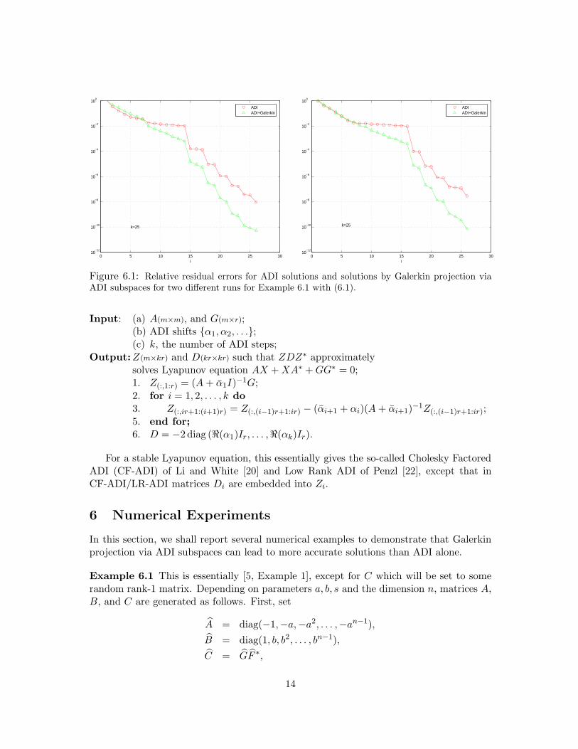
Figure 6.3: Relative residual errors for ADI solutions and solutions by Galerkin projection viaADI subspaces. Left: FOM in [8]; Right: HEAT in [8].

taken, and thus both E and F have 34 values among which 25 are selected in the end. OurfADI produces an approximation Xk = ZkDkY

∗k , along with intermediate approximations

Xi = ZiDiY∗i for i ≤ k. For two runs with different random F and G, Figures 6.1 and 6.2

plot the relative residual errors

‖AXi − XiB − GF ∗‖F

‖GF ∗‖F

(marked as “ADI”), as well as the relative residual errors for the approximations UiWiV∗i

by Galerkin projection (4.2) (marked as “ADI+Galerkin”). We have run tests on eachparameter set many times with different random F and G, and the residual behaviors areall similar to those plotted in Figures 6.1 and 6.2. In both figures, Galerkin projection viaADI subspaces produces better approximations after i ≥ 7 and the improvements are upto more than 2 decimal digits. ♦

Example 6.2 Chahlaoui and Van Dooren [8] compiled a collection of benchmark exam-ples for model reduction. Except those for descriptor systems, these examples give riseto Lyapunov equations AX + XA∗ + GG∗ = 0. Simplified versions of Algorithms 2.1and 3.1 upon substituting B = −A∗ and F = −G∗ can be applied. We have tested ADIand Galerkin projection via ADI subspaces on these equations, and found out both per-forms badly when A is highly non-normal in the sense that ‖A‖2

F and ‖A‖2F −

∑j |λj |2

are of the same magnitude and∑

j |λj |2 ≪ ‖A‖2F, where {λj} consists of all A’s eigen-

values. In the collection, there are two other examples whose A are in fact normal, i.e.,‖A‖2

F =∑

j |λj|2. We now report our numerical results on them. The first example isFOM: A = diag(A1, A2, A3, A4) with

A1 =

(−1 100−100 −1

), A2 =

(−1 200−200 −1

), A3 =

(−1 400

−400 −1

),

16

A4 = diag(−1,−2, . . . ,−1000), and G = (10, . . . , 10︸ ︷︷ ︸6

, 1, . . . , 1︸ ︷︷ ︸1000

)T. So n = 1006 and each

linear system with shifted A or A∗ takes O(n) flops to solve. Apply Algorithms 2.1 and3.1 with k = 66, where for Algorithm 3.1, each Arnoldi run takes 76 steps and 38 bestRitz values are taken, and thus E has 76 values among which 66 are selected in the end.The left of Figure 6.3 plots the relative residual errors for ADI solutions and solutions byGalerkin projection via ADI subspaces, as explained in Example 6.1. For this example,ADI barely does anything while projection ADI subspace method does extremely well.

The other example is from discretizing the 1-D heat equation. A is real symmetrictridiagonal. Thus each linear system with shifted A or A∗ takes O(n) flops to solve. Thesize of A can be made as large as one wishes. As in [8], we take n = 200, and A hasdiagonal entries −808 and off-diagonal entries 404, and all of G’s entries are zero, exceptG(67) = 1. With k = 20 for Algorithm 3.1, each Arnoldi run takes 30 steps and 15 bestRitz values are taken, and thus E has 30 values among which 20 are selected in the end.The right of Figure 6.3 plots the relative residual errors for ADI solutions and for solutionsby Galerkin projection via projection ADI subspaces method. ♦

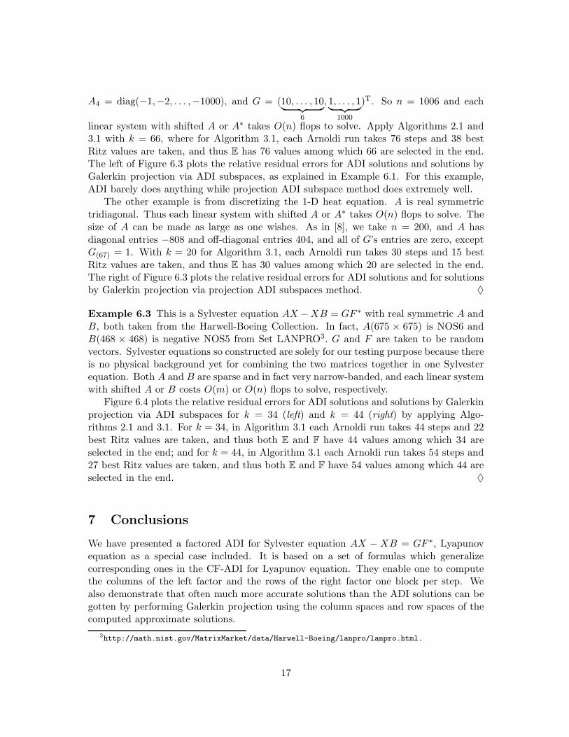
Example 6.3 This is a Sylvester equation AX −XB = GF ∗ with real symmetric A andB, both taken from the Harwell-Boeing Collection. In fact, A(675 × 675) is NOS6 andB(468 × 468) is negative NOS5 from Set LANPRO3. G and F are taken to be randomvectors. Sylvester equations so constructed are solely for our testing purpose because thereis no physical background yet for combining the two matrices together in one Sylvesterequation. Both A and B are sparse and in fact very narrow-banded, and each linear systemwith shifted A or B costs O(m) or O(n) flops to solve, respectively.

Figure 6.4 plots the relative residual errors for ADI solutions and solutions by Galerkinprojection via ADI subspaces for k = 34 (left) and k = 44 (right) by applying Algo-rithms 2.1 and 3.1. For k = 34, in Algorithm 3.1 each Arnoldi run takes 44 steps and 22best Ritz values are taken, and thus both E and F have 44 values among which 34 areselected in the end; and for k = 44, in Algorithm 3.1 each Arnoldi run takes 54 steps and27 best Ritz values are taken, and thus both E and F have 54 values among which 44 areselected in the end. ♦

7 Conclusions

We have presented a factored ADI for Sylvester equation AX − XB = GF ∗, Lyapunovequation as a special case included. It is based on a set of formulas which generalizecorresponding ones in the CF-ADI for Lyapunov equation. They enable one to computethe columns of the left factor and the rows of the right factor one block per step. Wealso demonstrate that often much more accurate solutions than the ADI solutions can begotten by performing Galerkin projection using the column spaces and row spaces of thecomputed approximate solutions.

3http://math.nist.gov/MatrixMarket/data/Harwell-Boeing/lanpro/lanpro.html.

17

0 5 10 15 20 25 30 3510

−7

10−6

10−5

10−4

10−3

10−2

10−1

100

k=34

i

ADIADI+Galerkin

0 5 10 15 20 25 30 35 40 4510

−9

10−8

10−7

10−6

10−5

10−4

10−3

10−2

10−1

100

k=44

i

ADIADI+Galerkin

Figure 6.4: Relative residual errors for ADI solutions and solutions by Galerkin projection viaADI subspaces for Example 6.3. Left: k = 34; Right: k = 44.

References

[1] N. I. Akhiezer, Elements of the Theory of Elliptic Functions, vol. 79 of Translationsof Mathematical Monographs, American Mathematical Soceity, Providence, RhodeIsland, 1990. translated from Russian by H. H. McFaden.

[2] A. C. Antoulas, Approximation of Large-Scale Dynamical Systems, Advances inDesign and Control, SIAM, Philadelphia, PA, 2005.

[3] A. C. Antoulas, D. C. Sorensen, and Y. Zhou, On the decay rate of hankelsingular values and related issues, Systems Control Lett., 46 (2002), pp. 323–342.

[4] R. H. Bartels and G. W. Stewart, Algorithm 432: The solution of the matrixequation AX − BX = C, Commun. ACM, 8 (1972), pp. 820–826.

[5] P. Benner, E. Quintana-Ortı, and G. Quintana-Ortı, Solving stable Sylvesterequations via rational iterative schemes, J. Sci. Comput., 28 (2006), pp. 51–83.

[6] R. Bhatia and P. Rosenthal, How and why to solve the operator equation AX −XB = Y , Bull. London Math. Soc., 29 (1997), pp. 1–21.

[7] D. Calvetti and L. Reichel, Application of ADI iterative methods to the restora-tion of noisy images, SIAM J. Matrix Anal. Appl., 17 (1996), pp. 165–186.

[8] Y. Chahlaoui and P. Van Dooren, A collection of benchmark examples for modelreduction of linear time invariant dynamical systems, SLICOT Working Notes 2002-2,February 2002. Available at www.win.tue.nl/niconet/NIC2/benchmodred.html.

[9] C. H. Choi and A. J. Laub, Efficient matrix-valued algorithm for solving stiffRiccati differential equations, IEEE Trans. Automat. Control, 35 (1990), pp. 770–776.

18

[10] L. Dieci, Numerical integration of the differential Riccati equation and some relatedissues, SIAM J. Numer. Anal., 29 (1992), pp. 781–815.

[11] N. S. Ellner and E. L. Wachspress, Alternating direction implicit iteration forsystems with complex spectra, SIAM J. Num. Anal., 3 (1991), pp. 859–870.

[12] G. H. Golub, S. Nash, and C. F. Van Loan, Hessenberg-Schur method for theproblem AX +XB = C, IEEE Trans. Automat. Control, AC-24 (1979), pp. 909–913.

[13] G. H. Golub and C. F. Van Loan, Matrix Computations, Johns Hopkins Univer-sity Press, Baltimore, Maryland, 3rd ed., 1996.

[14] L. Grasedyck, Existence of a low rank or H -matrix approximant to the solution ofa Sylvester equation, Numer. Linear Algebra Appl., 11 (2004), pp. 371–389.

[15] S. Gugercin, D. Sorensen, and A. Antoulas, A modified low-rank Smith methodfor large-scale, Numerical Algorithms, 32 (2003), pp. 27–55.

[16] D. Y. Hu and L. Reichel, Krylov-subspace methods for the Sylvester equation,Linear Algebra Appl., 172 (1992), pp. 283–313.

[17] I. M. Jaimoukha and E. M. Kasenally, Krylov subspace methods for solving largeLyapunov equations, SIAM J. Numer. Anal., 31 (1994), pp. 227–251.

[18] I. M. Jaimoukha and E. M. Kasenally, Oblique projectiob methods for large scalemodel reduction, SIAM J. Matrix Anal. Appl., 16 (1995), pp. 602–627.

[19] K. Jbilou, Low rank approximate solutions to large Sylvester matrix equations, Appl.Math. Comput., 177 (2006), pp. 365–376.

[20] J.-R. Li and J. White, Low-rank solution of Lyapunov equations, SIAM J. MatrixAnal. Appl., 24 (2002), pp. 260–280.

[21] , Low-rank solution of Lyapunov equations, SIAM Rev., 46 (2004), pp. 693–713.

[22] T. Penzl, A cyclic low-rank smith method for large sparse Lyapunov equations, SIAMJ. Sci. Comput., 21 (2000), pp. 1401–1418.

[23] , Eigenvalue decay bounds for solutions of Lyapunov equations: the symmetriccase, Systems Control Lett., 40 (2000), pp. 139–144.

[24] , LYAPACK: A MATLAB toolbox for large Lyapunov and Riccati equations,model reduction problems, and linear-quadratic optimal control problems, users’ guide(ver. 1.0). Available at www.tu-chemnitz.de/sfb393/lyapack/, 2000.

[25] Y. Saad, Numerical solution of large Lyapunov equations, in Signal Processing, Scat-tering, Operator Theory and Numerical Methods, M. A. Kaashoek, J. H. V. Shuppen,and A. Ran, eds., Birkhauser, Boston, MA, 1990, pp. 503–511.

19

[26] J. Sabino, Solution of Large-Scale Lyapunov Equations via the Block Modified SmithMethod, PhD thesis, Rice University, Houston, Texas, 2006.

[27] V. Simoncini, On the numerical solution of AX−XB = C, BIT, 36 (1996), pp. 814–830.

[28] , A new iterative method for solving large-scale Lyapunov matrix equations, SIAMJ. Sci. Comput., 29 (2007), pp. 1268–1288.

[29] N. Truhar and K. Veselic, Bounds on the trace of solution to the Lyapunovequation with a general stable matrix, Systems Control Lett., 56 (2007), pp. 493–503.

[30] E. L. Wachspress, Iterative solution of the Lyapunov matrix equation, Appl. Math.Lett., 1 (1988), pp. 87–90.

[31] E. L. Wachspress, The ADI Model Problem, Windsor, CA, 1995. Self-published(www.netlib.org/na-digest-html/96/v96n36.html).

[32] K. Zhou, J. C. Doyle, and K. Glover, Robust and Optimal Control, PrenticeHall, Upper Saddle River, New Jersey, 1995.

20