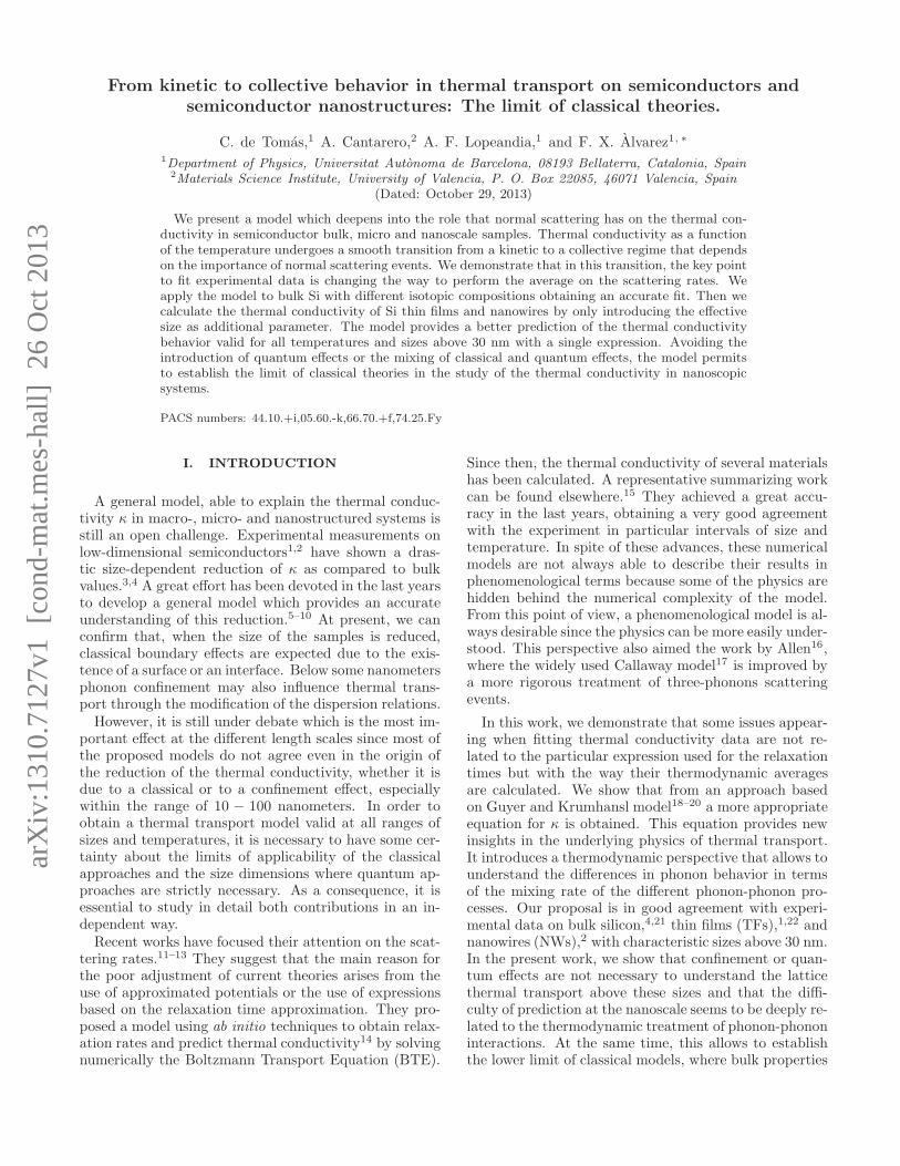
arX

iv:1

310.

7127

v1 [

cond

-mat

.mes

-hal

l] 2

6 O

ct 2

013

From kinetic to collective behavior in thermal transport on semiconductors and

semiconductor nanostructures: The limit of classical theories.

C. de Tomas,1 A. Cantarero,2 A. F. Lopeandia,1 and F. X. Alvarez1, ∗

1Department of Physics, Universitat Autonoma de Barcelona, 08193 Bellaterra, Catalonia, Spain2Materials Science Institute, University of Valencia, P. O. Box 22085, 46071 Valencia, Spain

(Dated: October 29, 2013)

We present a model which deepens into the role that normal scattering has on the thermal con-ductivity in semiconductor bulk, micro and nanoscale samples. Thermal conductivity as a functionof the temperature undergoes a smooth transition from a kinetic to a collective regime that dependson the importance of normal scattering events. We demonstrate that in this transition, the key pointto fit experimental data is changing the way to perform the average on the scattering rates. Weapply the model to bulk Si with different isotopic compositions obtaining an accurate fit. Then wecalculate the thermal conductivity of Si thin films and nanowires by only introducing the effectivesize as additional parameter. The model provides a better prediction of the thermal conductivitybehavior valid for all temperatures and sizes above 30 nm with a single expression. Avoiding theintroduction of quantum effects or the mixing of classical and quantum effects, the model permitsto establish the limit of classical theories in the study of the thermal conductivity in nanoscopicsystems.

PACS numbers: 44.10.+i,05.60.-k,66.70.+f,74.25.Fy

I. INTRODUCTION

A general model, able to explain the thermal conduc-tivity κ in macro-, micro- and nanostructured systems isstill an open challenge. Experimental measurements onlow-dimensional semiconductors1,2 have shown a dras-tic size-dependent reduction of κ as compared to bulkvalues.3,4 A great effort has been devoted in the last yearsto develop a general model which provides an accurateunderstanding of this reduction.5–10 At present, we canconfirm that, when the size of the samples is reduced,classical boundary effects are expected due to the exis-tence of a surface or an interface. Below some nanometersphonon confinement may also influence thermal trans-port through the modification of the dispersion relations.However, it is still under debate which is the most im-

portant effect at the different length scales since most ofthe proposed models do not agree even in the origin ofthe reduction of the thermal conductivity, whether it isdue to a classical or to a confinement effect, especiallywithin the range of 10 − 100 nanometers. In order toobtain a thermal transport model valid at all ranges ofsizes and temperatures, it is necessary to have some cer-tainty about the limits of applicability of the classicalapproaches and the size dimensions where quantum ap-proaches are strictly necessary. As a consequence, it isessential to study in detail both contributions in an in-dependent way.Recent works have focused their attention on the scat-

tering rates.11–13 They suggest that the main reason forthe poor adjustment of current theories arises from theuse of approximated potentials or the use of expressionsbased on the relaxation time approximation. They pro-posed a model using ab initio techniques to obtain relax-ation rates and predict thermal conductivity14 by solvingnumerically the Boltzmann Transport Equation (BTE).

Since then, the thermal conductivity of several materialshas been calculated. A representative summarizing workcan be found elsewhere.15 They achieved a great accu-racy in the last years, obtaining a very good agreementwith the experiment in particular intervals of size andtemperature. In spite of these advances, these numericalmodels are not always able to describe their results inphenomenological terms because some of the physics arehidden behind the numerical complexity of the model.From this point of view, a phenomenological model is al-ways desirable since the physics can be more easily under-stood. This perspective also aimed the work by Allen16,where the widely used Callaway model17 is improved bya more rigorous treatment of three-phonons scatteringevents.

In this work, we demonstrate that some issues appear-ing when fitting thermal conductivity data are not re-lated to the particular expression used for the relaxationtimes but with the way their thermodynamic averagesare calculated. We show that from an approach basedon Guyer and Krumhansl model18–20 a more appropriateequation for κ is obtained. This equation provides newinsights in the underlying physics of thermal transport.It introduces a thermodynamic perspective that allows tounderstand the differences in phonon behavior in termsof the mixing rate of the different phonon-phonon pro-cesses. Our proposal is in good agreement with experi-mental data on bulk silicon,4,21 thin films (TFs),1,22 andnanowires (NWs),2 with characteristic sizes above 30 nm.In the present work, we show that confinement or quan-tum effects are not necessary to understand the latticethermal transport above these sizes and that the diffi-culty of prediction at the nanoscale seems to be deeply re-lated to the thermodynamic treatment of phonon-phononinteractions. At the same time, this allows to establishthe lower limit of classical models, where bulk properties

2

are enough to understand the phenomenology. Only be-low this limit, of the order of a few tens of nanometers,quantum transport may play an important role.23

II. APPROACHES TO SOLVE THEBOLTZMANN TRANSPORT EQUATION

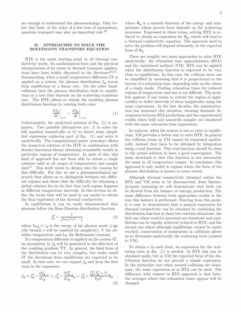
BTE is the usual starting point in all thermal con-ductivity works. Its mathematical form and the physicalinterpretation of its terms in thermal transport applica-tions have been widely discussed in the literature24,25.Summarizing, when a small temperature difference δT isapplied on a system, the phonon distribution fq movesfrom equilibrium at a linear rate. On the other hand,collisions turn the phonon distribution back to equilib-rium at a rate that depends on the scattering transitionrate. The BTE allows to obtain the resulting phonondistribution function by relating both rates

∂fq∂t

∣

∣

∣

∣

drift

=∂fq∂t

∣

∣

∣

∣

scatt

. (1)

Unfortunately, the analytical solution of Eq. (1) is un-known. Two possible alternatives are: i) to solve thefull equation numerically or ii) to derive some simpli-fied expression replacing part of Eq. (1) and solve itanalytically. The computational power nowadays allowsthe numerical solution of the BTE in combination withdensity functional theory obtaining remarkable results inparticular regions of temperature. In spite of this, thiskind of approach has not been able to obtain a singlesolution valid at all ranges of temperatures and samplesizes11. This work wants to deepen into the reasons forthis difficulty. For this we use a phenomenological ap-proach that allows us to distinguish between two differ-ent regimes and shows that the difficulty for obtaining aglobal solution lies in the fact that each regime happensat different temperature intervals. In this section we de-fine the terms that will be used in our model to obtainthe final expression of the thermal conductivity.In equilibrium it can be easily demonstrated that

phonons follow the Bose-Einstein distribution function

f0q=

1

e~ωq/kBT − 1, (2)

where ~ωq ≡ εq is the energy of the phonon mode (ν,q)(the branch ν will be omitted for simplicity), T the ab-solute temperature and kB the Boltzmann constant.If a temperature difference is applied on the system δT ,

an asymmetry in fq will be generated in the direction ofthe resulting gradient ∇T . In general, the final form ofthe distribution can be very complex, but under smallδT the deviations from equilibrium are expected to besmall. In that case, we can expand fq and keep the firstterm in the expansion:

fq ≃ f0q+

∂fq∂εq

δε ≃ f0q+

∂f0q

∂εqΦq = f0

q+

f0q(f0

q+ 1)

kBTΦq ,

(3)

where Φq is a smooth function of the energy and tem-perature whose precise form depends on the scatteringprocesses. Expressed in these terms, solving BTE is re-duced to obtain an expression for Φq, which will lead toa thermal conductivity equation. The approach used tosolve the problem will depend ultimately on the expectedform of Φq.

There are roughly two main approaches to solve BTEanalytically: the relaxation time approximation (RTA)and the variational method (VM). RTA can be appliedwhen the distribution function is expected to be veryclose to equilibrium. In this case, the collision term canbe simplified by assuming that it is proportional to theinverse of a relaxation time, depending only on the valuesof a single mode. Finding relaxation times for reducedregions of temperature and size is not difficult. The prob-lem appears if one wants to extend the region of appli-cability to wider intervals of these magnitudes using thesame expressions. In the last decades, the miniaturiza-tion has worsened this situation, showing dramatic di-vergences between RTA predictions and the experimentalresults when bulk and nanoscale samples are simulatedwith the same relaxation time expressions.

In contrast, when the system is not so close to equilib-rium, VM provides a better way to solve BTE. In generalthe collision terms in VM cannot be expressed analyti-cally, instead they have to be obtained by integrationusing a trial function. This trial function should be closeto the actual solution to have a good convergence. Themain drawback is that this function is not necessarilythe same in all temperature ranges. In conclusion, thisapproach is only useful in regions where the form of thephonon distribution is known to some extent.

Although thermal conductivity obtained within theRTA and VM seem to be disconnected, from thermo-dynamic reasoning we will demonstrate that both canbe derived from the balance of entropy production. Themain difference between both approaches resides in theway this balance is performed. Starting from this point,it is easy to demonstrate that a general expression forthermal conductivity can be obtained by combining thedistribution function in these two extreme situations: thefirst one where resistive processes are dominant and equi-librium can be rapidly achieved (related to RTA) and thesecond one where although equilibrium cannot be easilyreached, conservation of momentum in collisions allowsus to determine analytically the scattering term (relatedto VM).

To obtain κ in each limit, an expression for the scat-tering term in Eq. (1) is needed. In RTA this can beobtained easily, but in VM the expected form of the dis-tribution function do not provide a simple expression.In the particular case when normal collisions are domi-nant, the same expression as in RTA can be used. Thedifference with respect to RTA approach is that later,the averages where this relaxation times appear will bechanged.

3

A. Resistive vs Normal scattering (equilibrium vsnon-equilibrium)

As indicated before, the expected form of Φq will thedetermine the choice between a RTA or a VM approach.The calculation of the scattering rates depends on it and,at the same time this depends on which scattering mech-anism is dominating the system. Determining the domi-nating mechanism is thus the first important question tosolve.Phonons can relax by different mechanisms, colliding

with boundaries, impurities, electrons and between them.All these mechanisms are resistive except some part ofthe phonon-phonon collisions. Two phonons with wavenumber and energy (q, ωq) and (q′, ωq′) can scatter andproduce, as a result, a new phonon (q′′, ωq′′) (or vice-versa). In all events, energy must be conserved, but thewave number or quasi-momentum can be lost due to theinteraction with the whole lattice. The equation

q + q′ = q′′ +G, (4)

where G is a reciprocal lattice vector, expresses the factthat the total lattice can acquire an amount of momen-tum G because the resultant phonon is reflected outsideof the first Brillouin zone (BZ).25 If the quasi-momentumis conserved (G = 0) the scattering processes are callednormal or N-processes, while in the general case (G 6= 0)they are called Umklapp or U-processes. Regarding thedominance of the N-processes two limiting behaviors canbe considered:i) When resistive collisions are dominant and N-

processes are negligible, momentum will be completelydissipated and its average value is zero. The only wayto move the phonon distribution from equilibrium is bychanging its temperature. In that case, the distributionfunction takes the form

fq =1

e~ωq/kB(T+δT ) − 1≈

1

e~ωq/kBT e1−δT/T − 1. (5)

Comparing with Eq. (3) an expression for Φq can beobtained

Φq = ~ωq

δT

T. (6)

In this situation, RTA is the most useful approach to use.ii) When N-processes are dominant, the system will

not be able to relax the momentum to zero (the quasi-momentum is conserved) and a displacement u of thedistribution function in the direction of the thermal gra-dient is expected. The distribution function takes theform18

fq =1

e(~ωq−u·q)/kBT − 1(7)

which is in a non-equilibrium situation. Then, Φq takesthe form

Φq = u · q (8)

In this case the VM approach must be used.Summing up, Eqs. (6) and (8) are the two forms of Φq

used for the distribution function in each approach, RTAand VM respectively, corresponding to two extreme sit-uations described above. Next, we will use both expres-sions of Φq to show that in some situations, they yieldequivalent expressions for the relaxation times.

B. Defining Scattering rates

Once we have determined both expressions for Φq inthe two limiting cases, we can use them to determinethe collision term in Eq. (1) in each case. This dependson the transition probabilities and the form of the dis-tribution functions. In general, the collision term in theBoltzmann equation can be written, for elastic scatter-ing, as

∂fq∂t

∣

∣

∣

∣

scat

=

∫

Φq − Φq′

kBTP q

′

qdq′. (9)

where P q′

qare the scattering transition rates from mode

q to q′ when the distribution functions correspond toequilibrium.The integral (9) is expressing the fact that relaxation

process in an out of equilibrium is modified by termsΦq − Φq′ , i. e. depending on the displacement with re-spect to equilibrium of the different colliding particles.Expression (9) can be generalized for an arbitrary num-ber of colliding particles:

∂fq∂t

∣

∣

∣

∣

scat

=1

kBT

∫

Φq +

n∑

i=1

Φqi−

m∑

j=1

Φqj

Pq′

1..q′

mqq1...qn

m

n∏

i=1

j=1

dqidq′

j

(10)where q collides with {qi} giving as a result the modes{

q′

j

}

.In RTA we assume that the system is close enough

to equilibrium to express (10) only in terms of Φq. Forthis we can make the assumption that the only modeout of equilibrium is that with wave number q and theremaining modes rest in equilibrium. Thus

Φqi= Φq

′

j= 0 (11)

for all qi 6= q and q′

j 6= q. In this case,

∂fq∂t

∣

∣

∣

∣

scat

=Φq

kBT

∫

Pq′

1..q′

mqq1...qn

m

n∏

i=1

j=1

dqidq′

j (12)

If we substitute Eq. (3) in (12) we have

∂fq∂t

∣

∣

∣

∣

scat

=fq − f0

q

f0q(f0

q+ 1)

∫

Pq′

1..q′

mqq1...qn

m

n∏

i=1

j=1

dqidq′

j . (13)

4

Thus, we can define the relaxation time τq of mode q

as

1

τq=

1

f0q(f0

q+ 1)

∫

Pq′

1..q′

mqq1...qn

m

n∏

i=1

j=1

dqidq′

j (14)

and so, we obtain the BTE solution in the well knownRTA approach

∂fq∂t

∣

∣

∣

∣

scat

=fq − f0

q

τq. (15)

In VM condition (11) cannot be fulfilled and the col-lision integral (10) will be affected by the distribution ofthe rest of the participating modes Φqi

and Φq′

j. How-

ever, if normal scattering is the only relaxation process,assumption of (8) allows to simplify the final expression.In that case, since the integrand is an odd function of qiand we integrate in the whole momentum space,

∫

ΦqiP

q′

1..q′

mqq1...qndqi =

∫

Φq′

jP

q′

1..q′

mqq1...qndqi = 0 ∀i, j

(16)This condition leads to the same result as that obtainednear equilibrium (13)-(14), since condition (16) is equiva-lent to condition (11). Thus, we can use the same expres-sion for the scattering rates in both limiting situations,near equilibrium and in non-equilibrium, despite of thevery different nature of the two situations.In the following section we apply this result to obtain

an expression for the thermal conductivity under eachsituation. This will allow us to calculate two well differ-entiate regimes of behavior in the thermal transport: thekinetic and the collective regime.

III. THERMAL CONDUCTIVITY REGIMES

It is widely known that thermal conductivity in VMcan be derived from the balance of entropy25. In this sec-tion we use the same method to obtain the thermal con-ductivity for RTA in order to combine both approaches.Entropy variation can be calculated either from the

collision or from the drift term. The collision term isexpressed under a microscopic formalism, and the driftterm can be expressed in thermodynamic variables. Thekey point is that as normal scattering is the responsiblefor the mixing between modes, the balance between bothterms is affected by the strength of this scattering mech-anism. This is crucial to understand the discrepanciesbetween experiments and theoretical predictions.If mode mixing is low (N-processes are not important),

entropy balance should be fulfilled individually for everymode, that is, locally in momentum space. This leads tothe thermal conductivity in the kinetic regime. On theother hand, when mode mixing is high (N-processes dom-inate) the entropy balance should be achieved globally, in

that case we obtain the thermal conductivity in the col-

lective regime. Depending on the intensity of the normalcollisions we should select the local or the global versionfor the entropy production balance. Next, we detail bothregimes of behavior and obtain the corresponding ther-mal conductivity contribution.

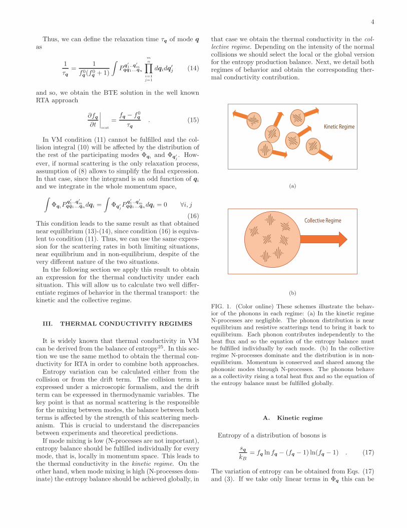
(a)

(b)

FIG. 1. (Color online) These schemes illustrate the behav-ior of the phonons in each regime: (a) In the kinetic regimeN-processes are negligible. The phonon distribution is nearequilibrium and resistive scatterings tend to bring it back toequilibrium. Each phonon contributes independently to theheat flux and so the equation of the entropy balance mustbe fulfilled individually by each mode. (b) In the collectiveregime N-processes dominate and the distribution is in non-equilibrium. Momentum is conserved and shared among thephononic modes through N-processes. The phonons behaveas a collectivity rising a total heat flux and so the equation ofthe entropy balance must be fulfilled globally.

A. Kinetic regime

Entropy of a distribution of bosons is

sqkB

= fq ln fq − (fq − 1) ln(fq − 1) . (17)

The variation of entropy can be obtained from Eqs. (17)and (3). If we take only linear terms in Φq this can be

5

written as25

sq|scat

=∂sq∂t

∣

∣

∣

∣

scat

=Φq

T

∂fq∂t

∣

∣

∣

∣

scat

, (18)

Thermodynamically, the entropy variation can be alsowritten in terms of the heat flux

sq|drift

=∂sq∂t

∣

∣

∣

∣

drift

= jq · ∇

(

1

T

)

=j2q

κqT 2(19)

where the heat flux of mode q is

jq = ~ωqvg(fq − f0q) = ~ωqvgf

0q(f0

q+ 1)

Φq

kBT(20)

and we have used the fact that jq = −κq∇T , where κq isthe thermal conductivity of mode q, and vg is the groupvelocity.Equating (19) and (18) leads to an expression giving

the thermal conductivity of each mode

κq =j2q

TΦq

∂fq∂t

∣

∣

∣

scat

. (21)

Integrating (21) over all modes yields total thermal con-ductivity in this kinetic regime

κkin =

∫

κqdq =

∫

j2q

TΦq

∂fq∂t

∣

∣

∣

scat

dq (22)

and if we substitute Eq. (20) we finally obtain

κkin =

∫

[

~ωqvgf0q(f0

q+ 1)

Φq

kBT

]2

TΦq

∂fq∂t

∣

∣

∣

scat

dq (23)

B. Collective regime

In the second limiting case, phonons behave as a col-lectivity. Now N-scattering dominates, and each modedo not contribute to thermal resistance individually butcollectively, so the balance of entropy should be achievedglobally. Thus, the total entropy production is on oneside

stot|scat =

∫

sq|scat

dq =

∫

Φq

T

∂fq∂t

∣

∣

∣

∣

scat

dq (24)

on the other side, we must account for a total heatflux, because in this regime thermal energy is distributedamong all the modes through normal scattering mech-anisms, this means that each mode does not carry anamount of heat flux independently, a global heat flux isthe result of the collective transport. Thus, a global en-tropy is produced

stot|drift = j2tot · ∇

(

1

T

)

(25)

and using the Fourier’s law jtot = −κ∇T , we obtain

stot|drift =j2totκT 2

. (26)

being κ the global thermal conductivity achieved in thisregime, we denote it as κcoll and we obtain its expressionby equating (24) and (26)

κcoll =j2tot

T 2∫ Φq

T∂fq∂t

∣

∣

∣

scat

dq(27)

where the total heat flux is

jtot =

∫

jqdq =

∫

~ωqvgf0q(f0

q+ 1)

Φq

Tdq (28)

By substituting this expression in Eq. (27), we have

κcoll =

[

∫

~ωqvgf0q(f0

q+ 1)

Φq

kBT dq]2

T 2∫ Φq

T∂fq∂t

∣

∣

∣

scat

dq(29)

After deducing the expression of the thermal conduc-tivity in each regime, we need to choose a magnitude ableto determine if we are in the local or global behavior. Sec-ondly in order to calculate the integrals in (23) and (29),we need some expressions for the collision terms. Thiswill be done in the next section.

IV. THERMAL CONDUCTIVITY IN TERMSOF FREQUENCY AND RELAXATION TIMES

We are now able to calculate the thermal conductiv-ity from Eq. (23) for RTA and from Eq. (29) for VM.In order to obtain numerical results for the thermal con-ductivity in both regimes, κkin and κcoll, first we need toexpress Φq in terms of the derivative of the distribution

function according to Eq. (3), and to express∂fq∂t

∣

∣

∣

scat

in

terms of the scattering rate according to Eq. (15). Thencombining all these equations in Eq. (23) in the kineticregime κkin can be rewritten as

κkin =

∫

~ωqτqv2g

∂f0q

∂Tdq (30)

which is the classical kinetic expression for the thermalconductivity.In the collective regime for (29), one can also com-

bine Eqs. (3) and (15), reminding that conditions (11)and (16) provide the same relaxation times expressionsin both approaches, RTA and VM. Then, κcoll can berewritten as

κcoll =

(

∫

Φqvg∂f0

q

∂T dq)2

∫ Φ2q

~ωq

1τq

∂f0q

∂T dq. (31)

6

κkin and κcoll can be re-expressed in terms of frequencyto simplify the integration in isotropic materials. Thisis done by the substitution dq → Dωdω , being Dω thedensity of states (DOS), and integrating the angular part.For the kinetic regime this leads to the expression

κkin =1

3

∫

~ωτωv2g

∂f0ω

∂TDωdω (32)

where now the frequency dependency is indicated withthe subindex (in the group velocity the subindex is omit-ted for simplicity), and for the collective regime

κcoll =1

3

(

∫

vgqω∂f0

ω

∂T Dωdω)2

∫ q2ω~ω

1τω

∂f0ω

∂T Dωdω(33)

where we have used the explicit form (8) to express Φq

in terms of the wave vector qω. The only question tobe addressed in Eq. (33) is that in order to maintainisotropy, q2ω should be a frequency averaged value. Thisdoes not lead to large variations in isotropic materials.As we have already pointed, in both expression (32)

and (33) τω is the same and accounts for the total relax-ation time contributing to thermal resistance. Then, wedenominate it τRω

. Finally, we need a magnitude whichaccounts for the kind of regime the phonon distributionis undergoing at the different temperatures. As we havecommented, this is determined by the degree of mixingbetween modes. Since this is related to the dominanceof normal with respect to resistive processes, a switch-ing factor weighting the relative importance of these pro-cesses should be used. This factor can be calculated froma matrix representation20

Σ ≡1

1 + <τN><τR>

(34)

where τN is the relaxation time due to N-processes andτR is the relaxation time due to resistive processes. Bothrelaxation times τN and τR are averaged over all modes.This is calculated as

〈τi〉 =

∫

~ωτiω∂f0

ω

∂T dq∫

~ω∂f0

ω

∂T dq(35)

with subindex i indicating N or R.The general expression of the thermal conductivity

must include this switching factor to account for all theintermediate regimes between the limiting regimes, i. e.from kinetic to collective regime. Thus,

κ = κkin(1− Σ) + κcollΣ (36)

If we are in the kinetic (unmixed-mode) limit τN >>τR then Σ → 0 and κ → κkin. If we are in the collective(mixed-mode) limit τN << τR then Σ → 1 and κ → κcoll.From Eq. (36) it can be deduced why all models based

on a single approach (RTA or VM) fail when extended

to a global model in a large range of temperatures. Inthis extension they are used in an approximation wherethey are not supposed to be valid. With this Eq. (36),the behavior change is included in the model, extendingits applicability to the whole temperature range.

A. Size-effects on the kinetic and collective terms

In a bulk semiconductor sample at near room temper-ature one can consider that only impurities scatteringand umklapp scattering participate significantly, then bymeans of the Mathiessen’s rule

τ−1Rω

= τ−1Iω

+ τ−1Uω

. (37)

If the dimension of the system is extremely reduced orthe temperatures are very low, intrinsic relaxation timescan be larger than the size of the system. In this case,boundary effects need to be included.In the kinetic regime of the thermal conductivity, as

the phonons behave individually, each mode could ex-perience independently a scattering with the boundary.Then, an extra term considering this effect should be in-cluded in the kinetic term of Eq. (36) by using the Math-iessen’s rule in combination with the intrinsic events, thisis τBω

the relaxation time due to boundary scattering

τ−1Rω

= τ−1Iω

+ τ−1Uω

+ τ−1Bω

. (38)

However, in the collective term some caution has tobe taken. In this regime a scattering rate is a quantitydescribing the distribution globally. In other words, onecannot assume an extra scattering term in each modeindependently because the boundary is noticed by thewhole phonon collectivity. Thermodynamically, this isthe same situation as flow on a pipe. Carriers in the cen-ter of the pipe notice the boundary not by themselvesbut through the collisions with the rest of the particles.The net effect on the flow is the reduction of the flowon the surface. The usual solution for this situation isto assume that the flow on the surface is zero. Thisis feasible if surfaces are rough enough. Once imposedthis extra assumption, a geometrical factor F dependingon the roughness and the transversal size of the systemshould be included in the collective term of Eq. (36). Inthe work by Guyer and Krumhansl20 this factor is calcu-lated for a cylindrical shape. In order to generalize thegeometrical factor to account for several geometries andso extend the range of validity of the collective term frombulk to small size samples, we used an expression derivedin a previous work26

F (Leff) =1

2π2

L2eff

ℓ2

(√

1 + 4π2ℓ2

L2eff

− 1

)

, (39)

being ℓ the phonon mean free path and Leff is the effec-tive length of the system. By geometrical considerations

7

it can be deduced25,27 that Leff = d for nanowires of di-ameter d, Leff =

√

π/2L for square wires of size L andLeff = 2.25h for thin layers of thickness h. Expression(39) was obtained in the framework of the Extended Ir-reversible Thermodynamics28 and includes in its deriva-tion higher order terms into the BTE expansion, whichcan be important when the size of the samples are ofthe order of the phonon mean free path and it has someadvantages: it is analytical, it can be used for differentgeometries and it takes automatically into considerationthe degree of non-equilibrium present in the sample de-pending on the normal and resistive relaxation times. Re-garding the mean free path, from the works by Alvarezet al.26 and Guyer-Krumhansl20 it can be easily deduced

that ℓ = vg

√

〈τN 〉〈τ−1R 〉−1, reminding that mean relax-

ation times are calculated from Eq. (35).Finally, the thermal conductivity for small size samples

would be

κ = κkin(1− Σ) + κcollΣF (Leff) (40)

Note that if ℓ → Leff , then F (Leff) → 1 and we recoverEq. (36).Next, we will test the validity of our model by ap-

plying it on different silicon samples since Si is a well-characterized semiconductor in the literature. This re-quires to calculate previously its dispersion relations,DOS, and relaxation times.

V. SILICON DISPERSION RELATIONS ANDDENSITY OF STATES

The bond charge model (BCM) proposed by Weber29

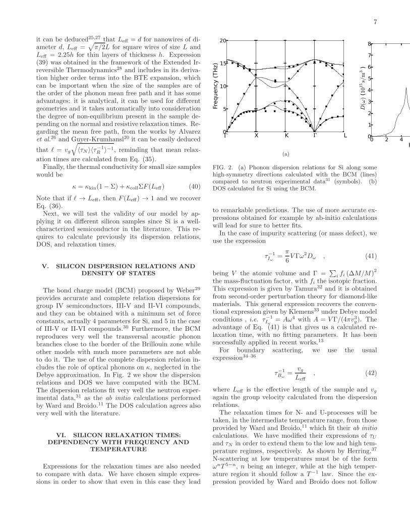
provides accurate and complete relation dispersions forgroup IV semiconductors, III-V and II-VI compounds,and they can be obtained with a minimum set of forceconstants, actually 4 parameters for Si, and 5 in the caseof III-V or II-VI compounds.30 Furthermore, the BCMreproduces very well the transversal acoustic phononbranches close to the border of the Brillouin zone whileother models with much more parameters are not ableto do it. The use of the complete dispersion relation in-cludes the role of optical phonons on κ, neglected in theDebye approximation. In Fig. 2 we show the dispersionrelations and DOS we have computed with the BCM.The dispersion relations fit very well the neutron exper-imental data,31 as the ab initio calculations performedby Ward and Broido.11 The DOS calculation agrees alsovery well with the literature.

VI. SILICON RELAXATION TIMES:DEPENDENCY WITH FREQUENCY AND

TEMPERATURE

Expressions for the relaxation times are also neededto compare with data. We have chosen simple expres-sions in order to show that even in this case they lead

Γ X0

5

10

15

20

Frequency (THz)

K Γ L

(a)

0 2 4 6 8 10 12 14 16 Frequency (THz)

0

1

2

3

4

5

6

7

8

D(ω

) (1015s/m

3)

FIG. 2. (a) Phonon dispersion relations for Si along somehigh-symmetry directions calculated with the BCM (lines)compared to neutron experimental data31 (symbols). (b)DOS calculated for Si using the BCM.

to remarkable predictions. The use of more accurate ex-pressions obtained for example by ab-initio calculationswill lead for sure to better fits.In the case of impurity scattering (or mass defect), we

use the expression

τ−1Iω

=π

6V Γω2Dω , (41)

being V the atomic volume and Γ =∑

i fi (∆M/M)2

the mass-fluctuation factor, with fi the isotopic fraction.This expression is given by Tamura32 and it is obtainedfrom second-order perturbation theory for diamond-likematerials. This general expression recovers the conven-tional expression given by Klemens33 under Debye modelconditions , i.e. τ−1

Iω= Aω4 with A = V Γ/(4πv3g). The

advantage of Eq. (41) is that gives us a calculated re-laxation time, with no fitting parameters. It has beensuccessfully applied in recent works.13

For boundary scattering, we use the usualexpression34–36

τ−1Bω

=vgLeff

, (42)

where Leff is the effective length of the sample and vgagain the group velocity calculated from the dispersionrelations.The relaxation times for N- and U-processes will be

taken, in the intermediate temperature range, from thoseprovided by Ward and Broido,11 which fit their ab initio

calculations. We have modified their expressions of τUand τN in order to extend them to the low and high tem-perature regimes, respectively. As shown by Herring,37

N-scattering at low temperatures must be of the formωnT 5−n, n being an integer, while at the high temper-ature region it should follow a T−1 law. Since the ex-pression provided by Ward and Broido does not follow

8

the right temperature dependence at high temperatures,we have included the additional term 1/(B′

NT ). In thisway, the expression will be valid in the whole tempera-ture range

τNω=

1

B′

NT+

1

BNT 3ω2[1− exp(−3T/ΘD)]. (43)

where ΘD is the Debye temperature. Concerning U-processes, following the argument provided by Ziman,25

at low temperatures the scattering of two phonons withwave vectors q1 and q2 cannot provide q3 + G, withG 6= 0, since low temperature means low energy or lowqi. In other words, U-processes are not possible at lowtemperature. We have established a temperature limitassuming that, for qU = 2π/3a (a being the lattice pa-rameter of Si), 1/3 the limit of the Brillouin zone, theprobability of U-processes decreases exponentially. Thetemperature limit ΘU is calculated through the expres-sion ~ωqU

≈ kBΘU . For Si we obtain ΘU ≈ 100 K. Thefinal expression for U-processes is:

τUω=

exp(ΘU/T )

BUω4T [1− exp(−3T/ΘD)]. (44)

At high enough temperatures, the numerator of Eq. (44)is 1 and we recover Ward and Broido’s expression.

VII. RESULTS AND DISCUSSION

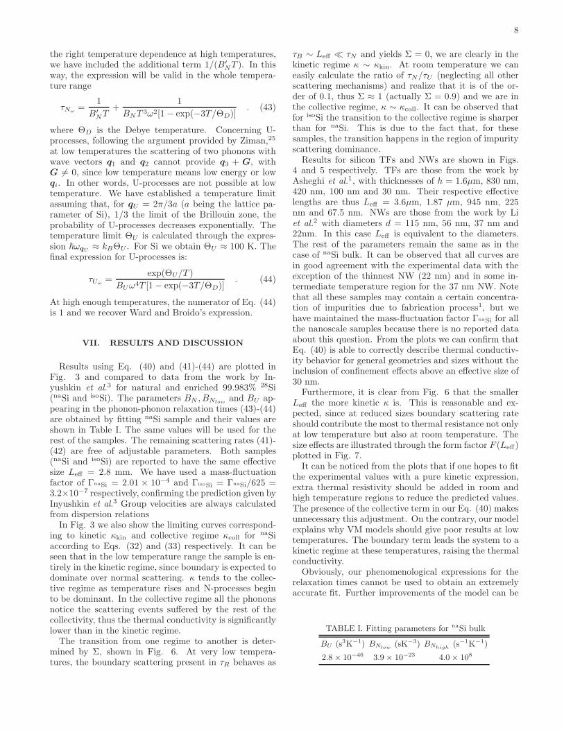
Results using Eq. (40) and (41)-(44) are plotted inFig. 3 and compared to data from the work by In-yushkin et al.3 for natural and enriched 99.983% 28Si(naSi and isoSi). The parameters BN , BNlow

and BU ap-pearing in the phonon-phonon relaxation times (43)-(44)are obtained by fitting naSi sample and their values areshown in Table I. The same values will be used for therest of the samples. The remaining scattering rates (41)-(42) are free of adjustable parameters. Both samples(naSi and isoSi) are reported to have the same effectivesize Leff = 2.8 mm. We have used a mass-fluctuationfactor of ΓnaSi = 2.01 × 10−4 and ΓisoSi = ΓnaSi/625 =3.2×10−7 respectively, confirming the prediction given byInyushkin et al.3 Group velocities are always calculatedfrom dispersion relationsIn Fig. 3 we also show the limiting curves correspond-

ing to kinetic κkin and collective regime κcoll for naSiaccording to Eqs. (32) and (33) respectively. It can beseen that in the low temperature range the sample is en-tirely in the kinetic regime, since boundary is expected todominate over normal scattering. κ tends to the collec-tive regime as temperature rises and N-processes beginto be dominant. In the collective regime all the phononsnotice the scattering events suffered by the rest of thecollectivity, thus the thermal conductivity is significantlylower than in the kinetic regime.The transition from one regime to another is deter-

mined by Σ, shown in Fig. 6. At very low tempera-tures, the boundary scattering present in τR behaves as

τB ∼ Leff ≪ τN and yields Σ = 0, we are clearly in thekinetic regime κ ∼ κkin. At room temperature we caneasily calculate the ratio of τN/τU (neglecting all otherscattering mechanisms) and realize that it is of the or-der of 0.1, thus Σ ≈ 1 (actually Σ = 0.9) and we are inthe collective regime, κ ∼ κcoll. It can be observed thatfor isoSi the transition to the collective regime is sharperthan for naSi. This is due to the fact that, for thesesamples, the transition happens in the region of impurityscattering dominance.Results for silicon TFs and NWs are shown in Figs.

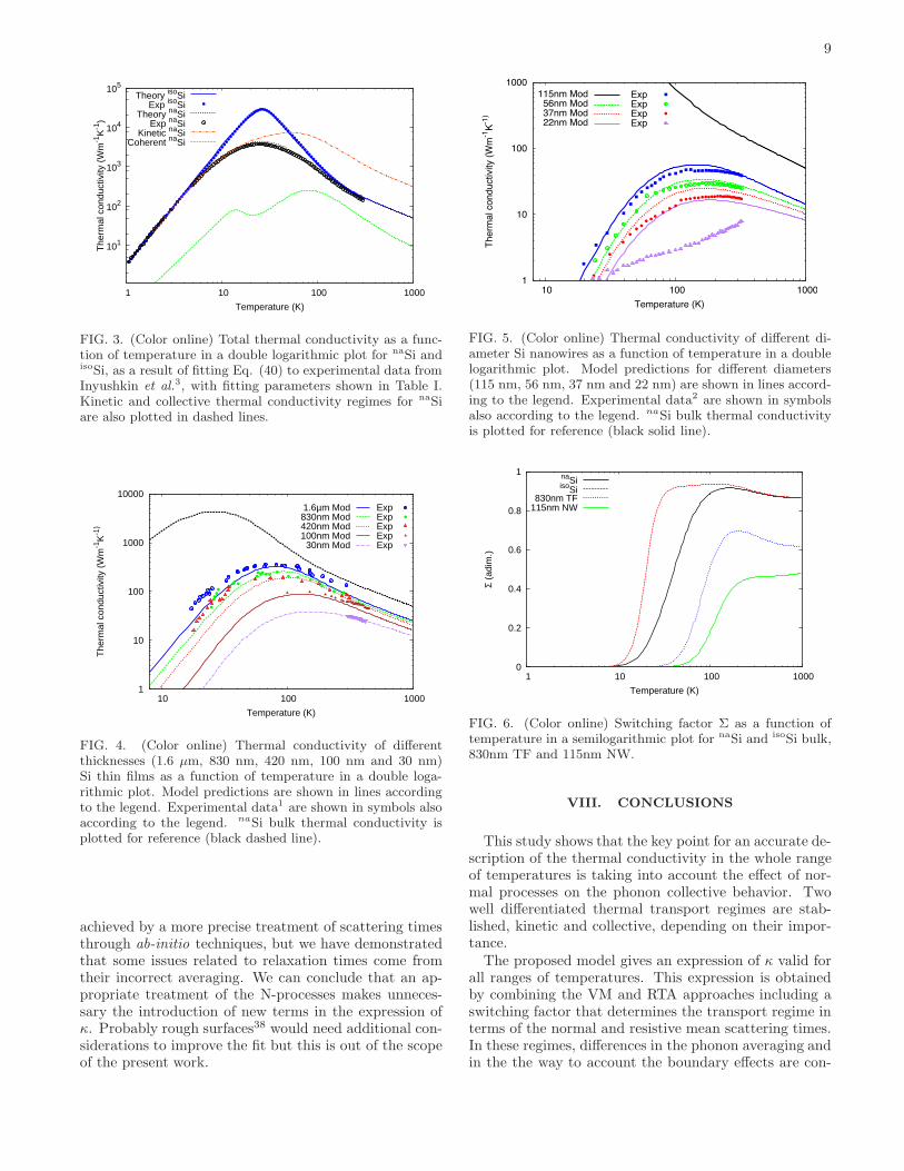
4 and 5 respectively. TFs are those from the work byAsheghi et al.1, with thicknesses of h = 1.6µm, 830 nm,420 nm, 100 nm and 30 nm. Their respective effectivelengths are thus Leff = 3.6µm, 1.87 µm, 945 nm, 225nm and 67.5 nm. NWs are those from the work by Liet al.2 with diameters d = 115 nm, 56 nm, 37 nm and22nm. In this case Leff is equivalent to the diameters.The rest of the parameters remain the same as in thecase of naSi bulk. It can be observed that all curves arein good agreement with the experimental data with theexception of the thinnest NW (22 nm) and in some in-termediate temperature region for the 37 nm NW. Notethat all these samples may contain a certain concentra-tion of impurities due to fabrication process1, but wehave maintained the mass-fluctuation factor ΓnaSi for allthe nanoscale samples because there is no reported dataabout this question. From the plots we can confirm thatEq. (40) is able to correctly describe thermal conductiv-ity behavior for general geometries and sizes without theinclusion of confinement effects above an effective size of30 nm.Furthermore, it is clear from Fig. 6 that the smaller

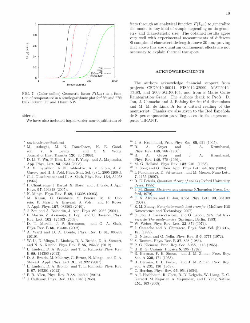
Leff the more kinetic κ is. This is reasonable and ex-pected, since at reduced sizes boundary scattering rateshould contribute the most to thermal resistance not onlyat low temperature but also at room temperature. Thesize effects are illustrated through the form factor F (Leff)plotted in Fig. 7.It can be noticed from the plots that if one hopes to fit

the experimental values with a pure kinetic expression,extra thermal resistivity should be added in room andhigh temperature regions to reduce the predicted values.The presence of the collective term in our Eq. (40) makesunnecessary this adjustment. On the contrary, our modelexplains why VM models should give poor results at lowtemperatures. The boundary term leads the system to akinetic regime at these temperatures, raising the thermalconductivity.Obviously, our phenomenological expressions for the

relaxation times cannot be used to obtain an extremelyaccurate fit. Further improvements of the model can be

TABLE I. Fitting parameters for naSi bulk

BU (s3K−1) BNlow(sK−3) BNhigh

(s−1K−1)

2.8× 10−46 3.9× 10−23 4.0× 108

9

101

102

103

104

105

1 10 100 1000

The

rmal

con

duct

ivity

(W

m-1

K-1

)

Temperature (K)

Theory isoSiExp isoSi

Theory naSiExp naSi

Kinetic naSiCoherent naSi

FIG. 3. (Color online) Total thermal conductivity as a func-tion of temperature in a double logarithmic plot for naSi andisoSi, as a result of fitting Eq. (40) to experimental data fromInyushkin et al.3, with fitting parameters shown in Table I.Kinetic and collective thermal conductivity regimes for naSiare also plotted in dashed lines.

1

10

100

1000

10000

10 100 1000

The

rmal

con

duct

ivity

(W

m-1

K-1

)

Temperature (K)

1.6µm Mod830nm Mod420nm Mod100nm Mod

30nm Mod

ExpExpExpExpExp

FIG. 4. (Color online) Thermal conductivity of differentthicknesses (1.6 µm, 830 nm, 420 nm, 100 nm and 30 nm)Si thin films as a function of temperature in a double loga-rithmic plot. Model predictions are shown in lines accordingto the legend. Experimental data1 are shown in symbols alsoaccording to the legend. naSi bulk thermal conductivity isplotted for reference (black dashed line).

achieved by a more precise treatment of scattering timesthrough ab-initio techniques, but we have demonstratedthat some issues related to relaxation times come fromtheir incorrect averaging. We can conclude that an ap-propriate treatment of the N-processes makes unneces-sary the introduction of new terms in the expression ofκ. Probably rough surfaces38 would need additional con-siderations to improve the fit but this is out of the scopeof the present work.

1

10

100

1000

10 100 1000

Th

erm

al co

nd

uctivity (

Wm

-1K

-1)

Temperature (K)

115nm Mod56nm Mod37nm Mod22nm Mod

ExpExpExpExp

FIG. 5. (Color online) Thermal conductivity of different di-ameter Si nanowires as a function of temperature in a doublelogarithmic plot. Model predictions for different diameters(115 nm, 56 nm, 37 nm and 22 nm) are shown in lines accord-ing to the legend. Experimental data2 are shown in symbolsalso according to the legend. naSi bulk thermal conductivityis plotted for reference (black solid line).

0

0.2

0.4

0.6

0.8

1

1 10 100 1000

Σ (a

dim

.)

Temperature (K)

naSiisoSi

830nm TF115nm NW

FIG. 6. (Color online) Switching factor Σ as a function oftemperature in a semilogarithmic plot for naSi and isoSi bulk,830nm TF and 115nm NW.

VIII. CONCLUSIONS

This study shows that the key point for an accurate de-scription of the thermal conductivity in the whole rangeof temperatures is taking into account the effect of nor-mal processes on the phonon collective behavior. Twowell differentiated thermal transport regimes are stab-lished, kinetic and collective, depending on their impor-tance.The proposed model gives an expression of κ valid for

all ranges of temperatures. This expression is obtainedby combining the VM and RTA approaches including aswitching factor that determines the transport regime interms of the normal and resistive mean scattering times.In these regimes, differences in the phonon averaging andin the the way to account the boundary effects are con-

10

0

0.2

0.4

0.6

0.8

1

1 10 100 1000

F(L

eff)

(adi

m.)

Temperature (K)

naSiisoSi

830nm TF115nm NW

FIG. 7. (Color online) Geometric factor F (Leff) as a func-tion of temperature in a semilogarithmic plot fornaSi and isoSibulk, 830nm TF and 115nm NW.

sidered.We have also included higher-order non-equilibrium ef-

fects through an analytical function F (Leff) to generalizethe model to any kind of sample depending on its geom-etry and characteristic size. The obtained results agreevery well with experimental measurements of differentSi samples of characteristic length above 30 nm, provingthat above this size quantum confinement effects are notnecessary to explain thermal transport.

ACKNOWLEDGMENTS

The authors acknowledge financial support fromprojects CSD2010-00044, FIS2012-32099, MAT2012-33483, and 2009-SGR00164, and from a Marie CurieReintegration Grant. The authors thank to Profs. D.Jou, J. Camacho and J. Bafaluy for fruitful discussionsand M. M. de Lima Jr for a critical reading of themanuscript. Thanks are also given to the Red Espanolade Supercomputacion providing access to the supercom-puter TIRANT.

∗ xavier.alvarez@uab.cat1 M. Asheghi, M. N. Touzelbaev, K. E. Good-son, Y. K. Leung, and S. S. Wong,Journal of Heat Transfer 120, 30 (1998).

2 D. Li, Y. Wu, P. Kim, L. Shi, P. Yang, and A. Majumdar,App. Phys. Lett. 83, 2934 (2003).

3 A. V. Inyushkin, A. N. Taldenkov, A. M. Gibin, A. V.Gusev, and H. J. Pohl, Phys. Stat. Sol. (c) 1, 2995 (2004).

4 C. J. Glassbrenner and G. A. Slack, Phys. Rev. 134, A1058(1964).

5 P. Chantrenne, J. Barrat, X. Blase, and J.D.Gale, J. App.Phys. 97, 104318 (2005).

6 N. Mingo, Phys. Rev. B 68, 113308 (2003).7 M. Kazan, G. Guisbiers, S. Pereira, M. R. Cor-reia, P. Masri, A. Bruyant, S. Volz, and P. Royer,J. Appl. Phys. 107, 083503 (2010).

8 J. Zou and A. Balandin, J. App. Phys. 89, 2932 (2001).9 P. Martin, Z. Aksamija, E. Pop, and U. Ravaioli, Phys.Rev. Lett. 102, 125503 (2009).

10 D. T. Morelli, J. P. Heremans, and G. A. Slack,Phys. Rev. B 66, 195304 (2002).

11 A. Ward and D. A. Broido, Phys. Rev. B 81, 085205(2010).

12 W. Li, N. Mingo, L. Lindsay, D. A. Broido, D. A. Stewart,and N. A. Katcho, Phys. Rev. B 85, 195436 (2012).

13 L. Lindsay, D. A. Broido, and T. L. Reinecke, Phys. Rev.B 88, 144306 (2013).

14 D. A. Broido, M. Malorny, G. Birner, N. Mingo, and D. A.Stewart, Appl. Phys. Lett. 91, 231922 (2007).

15 L. Lindsay, D. A. Broido, and T. L. Reinecke, Phys. Rev.B 87, 165201 (2013).

16 P. B. Allen, Phys. Rev. B 88, 144302 (2013).17 J. Callaway, Phys. Rev. 113, 1046 (1958).

18 J. A. Krumhansl, Proc. Phys. Soc. 85, 921 (1965).19 R. A. Guyer and J. A. Krumhansl,

Phys. Rev. 148, 766 (1966).20 R. A. Guyer and J. A. Krumhansl,

Phys. Rev. 148, 778 (1966).21 M. G. Holland, Phys. Rev. 132, 2461 (1963).22 D. Song and G. Chen, Appl. Phys. Lett. 84, 687 (2004).23 I. Ponomareva, D. Srivastava, and M. Menon, Nano Lett.

7, 1155 (2007).24 R. E. Peierls, Quantum theory of solids (Oxford University

Press, 1955).25 J. M. Ziman, Electrons and phonons (Clarendon Press, Ox-

ford, 1979).26 F. X. Alvarez and D. Jou, Appl. Phys. Lett. 90, 083109

(2007).27 Z. M. Zhang, Nano/microscale heat transfer (McGraw-Hill

Nanoscience and Technology, 2007).28 D. Jou, J. Casas-Vazquez, and G. Lebon, Extended Irre-

versible Thermodynamics (Springer, Berlin, 1993).29 W. Weber, Phys. Rev. Lett. 33, 371 (1974).30 J. Camacho and A. Cantarero, Phys. Stat. Sol. (b) 215,

181 (1999).31 G. Nilsson and G. Nelin, Phys. Rev. B 6, 3777 (1972).32 S. Tamura, Phys. Rev. B 27, 858 (1983).33 P. G. Klemens, Proc. Roy. Soc. A 68, 1113 (1955).34 H. B. G. Casimir, Physica 5, 595 (1938).35 R. Berman, F. E. Simon, and J. M. Ziman, Proc. Roy.

Soc. A 220, 171 (1953).36 R. Berman, E. L. Foster, and J. M. Ziman, Proc. Roy.

Soc. A 231, 130 (1953).37 C. Herring, Phys. Rev. 95, 954 (1954).38 A. I. Hochbaum, R. Chen, R. D. Delgado, W. Liang, E. C.

Garnett, M. Najarian, A. Majumdar, and P. Yang, Nature451, 163 (2008).