from current clinical practice to all-optical microfluidic technology
230
1 Bio-analytics - from current clinical practice to all-optical microfluidic technology Samir Aoudjane University College London Submitted for the degree of Doctor of Philosophy April 6, 2016
-
Upload
khangminh22 -
Category
Documents
-
view
2 -
download
0
Transcript of from current clinical practice to all-optical microfluidic technology

1
Bio-analytics - from current clinical practice toall-optical microfluidic technology
Samir AoudjaneUniversity College London
Submitted for the degree of Doctor of Philosophy
April 6, 2016

2
I, Samir Aoudjane confirm that the work presented in this thesis is my own. Where infor-mation has been derived from other sources, I confirm that this has been indicated in thethesis.

3
AbstractThere are many instances in which one would measure biological systems along a tem-perature gradient. This is because thermodynamics dictate the dynamics of biologicalprocesses. Here, systems are engineered where thermodynamic changes in biologicalsystems are enacted by the use of optical heating. This optical heating allows the useof microfluidic analysis systems in making measurement of these changes. Furthermore,measurement of the temperature changes themselves are made remotely of the sample,utilizing optical techniques. Overall these methods results in measurement of changes inbiological systems, in relation to temperature change, using much lower volumes of valu-able samples and reagents, than in comparable commercially available systems.
Specifically the stability of a fluorescent protein was measured in a bespoke microfluidicdevice using all optical heating, enacted by use of a infra-red laser. By measuring thedecrease in fluorescence of that protein as it became thermally denatured. This wasperformed using a measured volume of 15nl which is many orders of magnitude less thanthat used in a commercially available system. Work is ongoing, to generalize this, to non-fluorescent proteins by measuring the change in intrinsic fluorescence of proteins, as afunction of temperature.
A key technology in which temperature changes are enacted in a biological system isPCR, here controlled cycling of temperature is performed to induce an exponential in-crease in the amount of a DNA target. This process underpins sequencing of DNA as itallows enough DNA for the sequence to be detected. A microfluidic device would beconstructed to perform PCR thermocycling using optical heating and thermometry. Priorto this a DNA sequencing study was conducted of the mutational patterns of HBV in aclinical scenario. This study would provide sample for, and would be used as a compari-son for the construction of a microfluidic all optical qPCR device.

4
0.0.1 Acknowledgements
I wish to acknowledge the support and advice of my supervisory team, those being Prof.Gabriel Aeppli, Prof. Paul Dalby & Prof. Anna Maria Geretti. Without their knowledge andmaterial support this work would not have been possible.
Where individuals have made specific scientific or technical contributions they havebeen acknowledged in the appropriate section.
More generally I would like to thank my family and friends for putting up with me through-out this process. In particular my friends who are fellow student scientists for providingcomradeship & support throughout: Jamie Heather, John Ambrose, Alex Menys, ShimonaStarling, Angela Barrett, Joe Bailey, Valerian Turbe, Natascha Kappeler & many more be-sides.
This work is for patient 729

Contents 5
ContentsPage
0.0.1 Acknowledgements . . . . . . . . . . . . . . . . . . . . . . . . . . . . . . 4
List of Figures 9
List of Tables 15
1 Chapter 1 Introduction and Literature review 19
1.1 Microfluidics & thermodynamics in biological systems . . . . . . . . . . . . . . 20
1.1.1 Background to microfluidics for studying biological systems . . . . . . 20
1.1.2 Thermodynamics in biological systems . . . . . . . . . . . . . . . . . . . 21
1.2 Optical thermo-regulation of microfluidic biological analysis systems . . . . . 23
1.2.1 Lasers and Fluorescence . . . . . . . . . . . . . . . . . . . . . . . . . . . 24
1.2.2 Optical thermometry . . . . . . . . . . . . . . . . . . . . . . . . . . . . . 28
1.2.3 Closed loop Optical heating by infra-red laser with PID control . . . . 39
1.2.4 Fluorescence signal extraction by use of lock-in amplifiers . . . . . . . 41
1.3 Measurements of protein stability versus temperature . . . . . . . . . . . . . . 44
1.3.1 Protein structure and stability over temperature . . . . . . . . . . . . . 45
1.3.2 Relevance of measurement of protein stability . . . . . . . . . . . . . . 46
1.3.3 Current protein stability measurement systems . . . . . . . . . . . . . . 49
1.3.4 The Green Fluorescent Protein . . . . . . . . . . . . . . . . . . . . . . . . 51
1.4 Mutation patterns of Hepatitis B Virus . . . . . . . . . . . . . . . . . . . . . . . . 52
1.4.1 The Hepatitis B virion and its replication cycle . . . . . . . . . . . . . . . 52
1.4.2 HBV epidemiology . . . . . . . . . . . . . . . . . . . . . . . . . . . . . . . 54
1.4.3 HIV/HBV co-infection . . . . . . . . . . . . . . . . . . . . . . . . . . . . . 56
1.4.4 HIV and HBV infection in Malawi . . . . . . . . . . . . . . . . . . . . . . . 57
1.4.5 Use of Lamivudine in the treatment of HIV & HBV . . . . . . . . . . . . . 57
1.4.6 HBsAg mutants . . . . . . . . . . . . . . . . . . . . . . . . . . . . . . . . . 60
1.4.7 Study of mutation patterns by DNA sequencing . . . . . . . . . . . . . 63
1.5 The quantitative Polymerase Chain Reaction in disease diagnostics . . . . . 69
1.5.1 The Polymerase Chain Reaction and quantitative Polymerase Chain
Reaction . . . . . . . . . . . . . . . . . . . . . . . . . . . . . . . . . . . . . 69
1.5.2 Limiting dilution PCR . . . . . . . . . . . . . . . . . . . . . . . . . . . . . . 73

6
1.5.3 Use of qPCR in a clinical context . . . . . . . . . . . . . . . . . . . . . . 75
1.5.4 Commercial qPCR systems . . . . . . . . . . . . . . . . . . . . . . . . . . 77
1.5.5 Fast small scale qPCR systems . . . . . . . . . . . . . . . . . . . . . . . . 78
2 Chapter 2 Materials & Methods 83
2.1 Measurement of TAMRA fluorescence Vs Temperature for optical thermometry 84
2.1.1 Basic Fluorimetry of TAMRA as a function of temperature . . . . . . . . 84
2.1.2 Measurement of TAMRA in a qPCR reaction as a function of temper-
ature . . . . . . . . . . . . . . . . . . . . . . . . . . . . . . . . . . . . . . . 85
2.2 Measurement of GFP stability as a function of temperature . . . . . . . . . . 90
2.2.1 GFP thermal stability system physical construction . . . . . . . . . . . . 90
2.2.2 GFP thermal stability system data analysis methodology . . . . . . . . 92
2.3 Analysis of HBV mutational patterns in a cohort of HIV co-infected Malawians 94
2.3.1 Study population . . . . . . . . . . . . . . . . . . . . . . . . . . . . . . . . 94
2.3.2 Population sequencing of HBV mutational patterns . . . . . . . . . . . 94
2.3.3 Viral load detection of samples by quantitative PCR . . . . . . . . . . 97
2.3.4 HBV quasispecies analysis by limiting dilution whole genome PCR . . 98
2.3.5 HBV quasispecies analysis by ’454’ Next Generation Sequencing . . . 101
2.3.6 HBV quasispecies analysis by ’Illumina’ Next Generation Sequencing 103
2.4 Design of an all optical microfluidic qPCR system for HBV mutational analysis 106
2.4.1 System design iteration 1 - confocal microscope based imaging plat-
form . . . . . . . . . . . . . . . . . . . . . . . . . . . . . . . . . . . . . . . . 106
2.4.2 System design iteration 2 - fluorescence microscope based imaging
platform . . . . . . . . . . . . . . . . . . . . . . . . . . . . . . . . . . . . . 106
2.4.3 System design iteration 3 - bespoke detection platform . . . . . . . . . 109
3 Chapter 3 Results of Protein stability measurements in nl range 119
3.1 Introduction to Results of Protein stability measurements in nl range . . . . . 120
3.2 Imaging of GFP and TAMRA fluorescence to deduce GFP denaturation as a
function of temperature also shows a time dependence of GFP denaturation120
3.3 Calculation of GFP denaturation from fluorescence signal decay rate . . . 125
3.4 Decay of GFP fluorescence in optically heated microfluidic device versus
traditional water bath heated fluorimeter . . . . . . . . . . . . . . . . . . . . . 128
4 Chapter 4 Results of HBV sequencing 133

Contents 7
4.1 Introduction to results of HBV sequencing . . . . . . . . . . . . . . . . . . . . . 134
4.2 Results of Sanger sequencing . . . . . . . . . . . . . . . . . . . . . . . . . . . . 134
4.3 Next generation Sequencing of HBV mutants by ’454’ deep sequencing . . 137
4.4 Next generation Sequencing of HBV mutants by ’Illumina’ deep sequencing 142
4.5 Analysis of HBV mutants by Single whole genome sequencing . . . . . . . . 148
5 Chapter 5 Results of IRqPCR system measurements 153
5.1 Introduction to Results of IRqPCR system measurements . . . . . . . . . . . . 154
5.2 First IRqPCR system iteration results . . . . . . . . . . . . . . . . . . . . . . . . . 154
5.2.1 Control qPCR reactions performed in commercial qPCR instrument to
verify qPCR reaction is functional . . . . . . . . . . . . . . . . . . . . . . 154
5.2.2 Inhibition of PCR by TAMRA . . . . . . . . . . . . . . . . . . . . . . . . . . 155
5.2.3 Amplification of DNA not detected . . . . . . . . . . . . . . . . . . . . . 157
5.3 Second IRqPCR system iteration results . . . . . . . . . . . . . . . . . . . . . . . 161
5.3.1 Temperature calibration curve for ’microwell’ sample holder . . . . . 161
5.3.2 PID feedback control facilitates tighter temperature regulation . . . . 163
5.3.3 Irreversible photo-bleaching prevents long term thermoregulation . . 168
5.4 Third IRqPCR system iteration results . . . . . . . . . . . . . . . . . . . . . . . . . 169
5.4.1 Temperature tracking by 3rd iteration IRqPCR system . . . . . . . . . . 169
5.4.2 Irreversible photobleaching does not appreciably affect thermo reg-
ulation or DNA binding dye readout . . . . . . . . . . . . . . . . . . . . 173
5.4.3 Failure to detect signal resultant from successful PCR in third iteration
IRqPCR system . . . . . . . . . . . . . . . . . . . . . . . . . . . . . . . . . 174
6 Chapter 6 Discussion & Conclusions 177
6.1 Overview to Conclusions . . . . . . . . . . . . . . . . . . . . . . . . . . . . . . . 178
6.2 Conclusions for results of protein stability measurements in nl range . . . . . 178
6.2.1 New system for the generalization of protein stability measurements
in the nl range . . . . . . . . . . . . . . . . . . . . . . . . . . . . . . . . . . 178
6.2.2 General system design renders and implementation . . . . . . . . . . 179
6.2.3 Test data from general system & future work . . . . . . . . . . . . . . . 183
6.3 Conclusions for results of HBV sequencing . . . . . . . . . . . . . . . . . . . . . 186
6.4 Conclusions for results of IRqPCR system measurements . . . . . . . . . . . . . 187
6.4.1 Possible reasons for failure of qPCR reaction . . . . . . . . . . . . . . . . 188
6.4.2 Plan for next system iteration . . . . . . . . . . . . . . . . . . . . . . . . . 189
8
7 Chapter 7 Commercialization 191
7.1 Overview to commercialization . . . . . . . . . . . . . . . . . . . . . . . . . . . 192
7.1.1 Commercial target space exploration . . . . . . . . . . . . . . . . . . . 192
7.1.2 IP appraisal . . . . . . . . . . . . . . . . . . . . . . . . . . . . . . . . . . . 193
7.1.3 Industrial partners & collaboration . . . . . . . . . . . . . . . . . . . . . 193
7.2 Commercialization of protein fluorescence measurement . . . . . . . . . . . 194
7.2.1 Micro-plate readers/ fluorescence spectrometers as a commercial
target . . . . . . . . . . . . . . . . . . . . . . . . . . . . . . . . . . . . . . . 194
7.2.2 Bio-process monitoring and optimization . . . . . . . . . . . . . . . . . . 196
7.2.3 Drug discovery pipeline operation . . . . . . . . . . . . . . . . . . . . . 197
7.3 Commercialization of all optical qPCR . . . . . . . . . . . . . . . . . . . . . . . 198
7.3.1 qPCR in a clinical and research commercial setting . . . . . . . . . . . 198
7.3.2 Point of care & home diagnostics . . . . . . . . . . . . . . . . . . . . . . 199
7.4 Summary of Commercialization strategy . . . . . . . . . . . . . . . . . . . . . . 202
Appendices 203
Appendix A Single genome analysis week 0 consensus sequence 205
Appendix B sequencing data all sample genotype data 207
3 Bibliography 213
List of Figures 9
List of Figures
1.1 A plot of the number of papers produced in the sub-fields of microfluidics
taken from Sackmann et. al. [Sackmann et al., 2014] . . . . . . . . . . . . . . 21
1.2 Diagrams of the energy states of a particle undergoing in A absorption B
spontaneous emission and C stimulated emission as it interacts with photons 25
1.3 The structure of the green fluorescent protein with the central chromophore
illustrated . . . . . . . . . . . . . . . . . . . . . . . . . . . . . . . . . . . . . . . . . 27
1.4 The structure of SYBR green I . . . . . . . . . . . . . . . . . . . . . . . . . . . . . 28
1.5 Schematic of a typical setup for heating some fluid sample for analysis . . . 29
1.6 A guide to the range of commercially available thermochromic pigments
from a single manufacturer . . . . . . . . . . . . . . . . . . . . . . . . . . . . . . 33
1.7 The structure of the TAMRA molecule . . . . . . . . . . . . . . . . . . . . . . . . 36
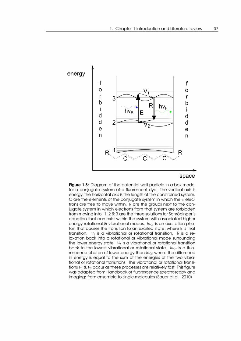
1.8 Diagram of the potential well particle in a box model for a conjugate system
of a fluorescent dye . . . . . . . . . . . . . . . . . . . . . . . . . . . . . . . . . . 37
1.9 A graphical representation of a typical PID control loop . . . . . . . . . . . . 39
1.10 Schematic of a experiment in which a lock-in amplifier is used to measure
low level fluorescence . . . . . . . . . . . . . . . . . . . . . . . . . . . . . . . . . 43
1.11 A schematic of the internal logic of a lock-in amplifier . . . . . . . . . . . . . 43
1.12 Classical and current methodology for producing enzymes for industrial pro-
cesses taken from kirk 2002 [Kirk et al., 2002] . . . . . . . . . . . . . . . . . . . . 47
1.13 The bio-catalysis cycle taken from Schmid 2001 [Schmid et al., 2001] . . . . 49
1.14 Demonstration of the varying size sample holders for biological analysis sys-
tems. . . . . . . . . . . . . . . . . . . . . . . . . . . . . . . . . . . . . . . . . . . . 51
1.15 Structure of the HBV genome taken from Lee 1997 [Lee, 1997] . . . . . . . . 53
1.16 Map showing the global distribution of HBV . . . . . . . . . . . . . . . . . . . . 55
1.17 Geographic distribution of HBV genotypes, where the size of the genotype
letter corresponds to the relative prevelance of HBV in that region, taken
from Pujol 2009 [Pujol et al., 2009] . . . . . . . . . . . . . . . . . . . . . . . . . . 56
1.18 Illustration of the overlapping reading frames at position 173 of ORF P and
164 of ORF S . . . . . . . . . . . . . . . . . . . . . . . . . . . . . . . . . . . . . . . 61
1.19 Illustration of the overlapping reading frames at position 204 of ORF P and
195 of ORF S . . . . . . . . . . . . . . . . . . . . . . . . . . . . . . . . . . . . . . . 61
10
1.20 The cost to sequence a human sized genome as a function of time . . . . . 63
1.21 A schematic of how the Illumina sequencing procedure operates taken
from Voelkerding et. al 2009[Voelkerding et al., 2009] . . . . . . . . . . . . . . 67
1.22 A schematic representation of the PCR process . . . . . . . . . . . . . . . . . 71
1.23 Schematic of FRET probe operation in qPCR . . . . . . . . . . . . . . . . . . . 73
1.24 Plot of the probability that a successfully amplified PCR reaction was derived
from a single piece of DNA as a function of the proportion of reactions that
failed to amplify due to no DNA template being present . . . . . . . . . . . . 75
2.1 TAMRA fluorescence as a function of temperature . . . . . . . . . . . . . . . 85
2.2 Titration of TAMRA concentration in qPCR reactions to gauge if TAMRA causes
a concentration dependent inhibition of qPCR readout . . . . . . . . . . . . 86
2.3 TAMRA fluorescence as a function of temperature in the same concentra-
tion as included in qPCR mix, and measured in a qPCR mix . . . . . . . . . . 87
2.4 Example data of temperature probe in modified cuvette to gain accurate
measurement of TAMRA fluorescence at a known concentration in a qPCR
reagent mix as a function of temperature . . . . . . . . . . . . . . . . . . . . . 89
2.5 Physical construction of GFP stability measurement system . . . . . . . . . . . 91
2.6 Imaging of GFP and TAMRA fluorescence do deduce GFP denaturation as
a function of temperature . . . . . . . . . . . . . . . . . . . . . . . . . . . . . . 93
2.7 Plate setup for limiting dilution whole genome PCR . . . . . . . . . . . . . . . 100
2.8 Photograph of the custom microscope mount that comprised the physical
construction on the second iteration of an all optical qPCR system . . . . . . 108
2.9 Schematic for the 3rd iteration of an all optical qPCR system . . . . . . . . . 110
2.10 A picture of the entire setup for the 3rd iteration of an all optical qPCR ma-
chine . . . . . . . . . . . . . . . . . . . . . . . . . . . . . . . . . . . . . . . . . . . 111
2.11 A picture of subsystem rail 1 of the third iteration of an all optical qPCR system113
2.12 A picture of subsystem rail 2 of the third iteration of an all optical qPCR system115
2.13 A picture of subsystem rail 4 of the third iteration of an all optical qPCR system116
2.14 A picture of subsystem rail 3 of the third iteration of an all optical qPCR system117
3.1 Time dependent plots of TAMRA and GFP fluorescence as infra-red heating
is initiated . . . . . . . . . . . . . . . . . . . . . . . . . . . . . . . . . . . . . . . . 122
3.2 GFP fluorescence is not completely recovered after heating and cooling
with infra-red laser . . . . . . . . . . . . . . . . . . . . . . . . . . . . . . . . . . . 124
List of Figures 11
3.3 GFP fluorescence is not lost after heating and cooling with infra-red laser, if
not heated past the tipping point of aggregation . . . . . . . . . . . . . . . . 125
3.4 Deduction of GFP denaturation rate from decay of GFP fluorescent intensity
at known temperatures . . . . . . . . . . . . . . . . . . . . . . . . . . . . . . . . 127
3.5 GFP fluorescence decay in optically heated microfluidic device Vs tradi-
tional water bath heated fluorimeter . . . . . . . . . . . . . . . . . . . . . . . . 129
3.6 A measurement of GFP fluoresence measured as a function of temperature
from [Bokman and Ward, 1981] . . . . . . . . . . . . . . . . . . . . . . . . . . . 131
3.7 A measurement of GFP fluoresence measured as a function of temperature
from iGEM Part:BBa_K515105 . . . . . . . . . . . . . . . . . . . . . . . . . . . . . 132
4.1 Schematic of the HBV polymerase mutants studied . . . . . . . . . . . . . . . 135
4.2 Pie chart representing the amino acid residues present at position 173 of the
reverse transcriptase of HBV as elucidated by ’454’ deep sequencing for the
the sample derived from patient 854 . . . . . . . . . . . . . . . . . . . . . . . . 140
4.3 Part 1 of pie charts representing the amino acid residues present at posi-
tion 204 of the reverse transcriptase of HBV as elucidated by ’454’ deep
sequencing . . . . . . . . . . . . . . . . . . . . . . . . . . . . . . . . . . . . . . . 141
4.4 Part 2 of pie charts representing the amino acid residues present at posi-
tion 204 of the reverse transcriptase of HBV as elucidated by ’454’ deep
sequencing . . . . . . . . . . . . . . . . . . . . . . . . . . . . . . . . . . . . . . . 142
4.5 Part one of graphical representation of the protein residues found a position
204 of the reverse transcriptase of HBV as elucidated by ’Illumina’ deep
sequencing. . . . . . . . . . . . . . . . . . . . . . . . . . . . . . . . . . . . . . . 144
4.6 Part two of graphical representation of the protein residues found a position
204 of the reverse transcriptase of HBV as elucidated by ’Illumina’ deep
sequencing . . . . . . . . . . . . . . . . . . . . . . . . . . . . . . . . . . . . . . . 146
4.7 A phylogenetic tree comparing sequences from the Sanger sequencing
and Illumina deep sequencing experiments . . . . . . . . . . . . . . . . . . . 148
4.8 A phyologentic tree in which the genetic distance between the full genomes
elucidated by full single gnenome sequencing are compared to other HBV
genotypes . . . . . . . . . . . . . . . . . . . . . . . . . . . . . . . . . . . . . . . . 151
5.1 Control qPCR reactions performed in commercial qPCR instrument to verify
qPCR reaction is functional . . . . . . . . . . . . . . . . . . . . . . . . . . . . . . 155

12
5.2 Agarose gel electrophoresis image of PCR reaction in presence/absence of
TAMRA . . . . . . . . . . . . . . . . . . . . . . . . . . . . . . . . . . . . . . . . . . 156
5.3 FAM probe fluorescence image and analysis prior to qPCR in iteration 1 system158
5.4 FAM probe fluorescence image and analysis subsequent to qPCR in iteration
1 system . . . . . . . . . . . . . . . . . . . . . . . . . . . . . . . . . . . . . . . . . 159
5.5 FAM probe fluorescence image and analysis subsequent to qPCR and with
manual mixing of sample in iteration 1 system . . . . . . . . . . . . . . . . . . . 160
5.6 Plot of calculated temperature values in ’microwell’ for a range of IR laser
power levels . . . . . . . . . . . . . . . . . . . . . . . . . . . . . . . . . . . . . . . 162
5.7 Plot of stabilized temperature values in ’microwell’ for a range of IR laser
power levels . . . . . . . . . . . . . . . . . . . . . . . . . . . . . . . . . . . . . . . 163
5.8 PID feedback control facilitates tighter temperature regulation at lower test
temperatures in the microwell sample holder geometry . . . . . . . . . . . . 164
5.9 At higher temperatures bubble formation in the microwell geometry causes
a catastrophic breakdown of system control . . . . . . . . . . . . . . . . . . . 165
5.10 Light microscopy image of the microwell sample holder . . . . . . . . . . . . 166
5.11 A montage of scanning electron micrographs of the microwell sample holder
taken at different angles and magnifications to assess surface quality of the
device . . . . . . . . . . . . . . . . . . . . . . . . . . . . . . . . . . . . . . . . . . 167
5.12 Complete thermocycling program completion in the capillary sample holder
configuration . . . . . . . . . . . . . . . . . . . . . . . . . . . . . . . . . . . . . . 168
5.13 First cycle only of temperature tracking by 3rd iteration IRqPCR system fol-
lowing a typical two step PCR thermocycling program . . . . . . . . . . . . . 170
5.14 Temperature tracking by 3rd iteration IRqPCR system following a typical two
step PCR thermocycling program . . . . . . . . . . . . . . . . . . . . . . . . . . 171
5.15 First cycle only of temperature tracking by 3rd iteration IRqPCR system fol-
lowing a typical three step PCR thermocycling program . . . . . . . . . . . . 172
5.16 Temperature tracking by 3rd iteration IRqPCR system following a typical three
step PCR thermocycling program . . . . . . . . . . . . . . . . . . . . . . . . . . 172
5.17 System does not increase power supply to IR laser during thermocycling pro-
cedure indicating that irreversible photobleaching of TAMRA is not affecting
temperature regulation of the system(rolling average for clarity) . . . . . . . 174
5.18 Increase in sybr green fluorescence is not detected in the third iteration sys-
tem despite apparently successful thermocycling . . . . . . . . . . . . . . . . 175
List of Figures 13
6.1 An example of the fluorescence excitation and emission spectra of Trypto-
phan . . . . . . . . . . . . . . . . . . . . . . . . . . . . . . . . . . . . . . . . . . . 179
6.2 A rendering of the overall design of the microfluidic UV time resolved protein
fluorescence measurement system . . . . . . . . . . . . . . . . . . . . . . . . . 180
6.3 An engineering drawing of the ’wedge’ mount used to constrain the sample
in the microfluidic UV time resolved protein fluorescence measurement system181
6.4 Qedge mount with sample capillary mounted . . . . . . . . . . . . . . . . . . 182
6.5 Render of wedge mount with sample capillary mounted in light path . . . . 182
6.6 Render of wedge mount with sample capillary mounted in light path . . . . 183
6.7 Plot of time resolved intrinsic fluorescence of concentrations of BSA, by the
UV time resolved protein fluorescence measurement system . . . . . . . . . 184
6.8 Infra red laser with new collimation optics . . . . . . . . . . . . . . . . . . . . . 185
6.9 The position of this combining optic is shown in a render of the system from
a top down view . . . . . . . . . . . . . . . . . . . . . . . . . . . . . . . . . . . . 186
6.10 A plot of the transmission of light at 1460nm through water as a function of
distance in microns . . . . . . . . . . . . . . . . . . . . . . . . . . . . . . . . . . . 189
7.1 An example of a "microplate reader" instrument . . . . . . . . . . . . . . . . . 193
7.2 An example of a cuvette . . . . . . . . . . . . . . . . . . . . . . . . . . . . . . . 195
7.3 An example of a microplate . . . . . . . . . . . . . . . . . . . . . . . . . . . . . 196
7.4 A mockup of a point of care all optical PCR system . . . . . . . . . . . . . . . 200
7.5 A mockup of a point of care all optical PCR system viewed isometrically . . 201
7.6 A mockup of a point of care all optical PCR system viewed isometrically . . 201
B.1 HBV virus genotype raw data for samples where only the first time point was
available . . . . . . . . . . . . . . . . . . . . . . . . . . . . . . . . . . . . . . . . 208
B.2 HBV virus genotype raw data for samples where the first and second time
points were available part 1 . . . . . . . . . . . . . . . . . . . . . . . . . . . . . 209
B.3 HBV virus genotype raw data for samples where the first and second time
points were available part 2 . . . . . . . . . . . . . . . . . . . . . . . . . . . . . 210
B.4 HBV virus genotype raw data for samples where all three time points were
available part 1 . . . . . . . . . . . . . . . . . . . . . . . . . . . . . . . . . . . . . 211
B.5 HBV virus genotype raw data for samples where all three time points were
available part 2 . . . . . . . . . . . . . . . . . . . . . . . . . . . . . . . . . . . . . 212

14

List of Tables 15
List of Tables1 List of abbreviations . . . . . . . . . . . . . . . . . . . . . . . . . . . . . . . . . . 17
1.1 The DNA codon table . . . . . . . . . . . . . . . . . . . . . . . . . . . . . . . . . 59
2.1 fitting parameters for calibration function for qPCR device . . . . . . . . . . . 88
2.2 Primers used for sanger sequencing of HBV polymerase sequences . . . . . 95
2.3 Table of reagent mixture used in the PCR reaction to amplify HBV poly-
merase for Sanger sequencing . . . . . . . . . . . . . . . . . . . . . . . . . . . . 95
2.4 Thermocycling program for HBV polymerase amplification leading to Sanger
sequencing . . . . . . . . . . . . . . . . . . . . . . . . . . . . . . . . . . . . . . . 96
2.5 Table of the constituents of the cycle sequencing reaction used in Sanger
sequencing of HBV polymerase . . . . . . . . . . . . . . . . . . . . . . . . . . . 96
2.6 cycle sequencing thermocycler program . . . . . . . . . . . . . . . . . . . . . 97
2.7 Primer and probe sequences used in qPCR of HBV polymerase . . . . . . . . 97
2.8 HBV pol qPCR reagent mixture . . . . . . . . . . . . . . . . . . . . . . . . . . . . 98
2.9 HBV limiting dilution whole genome PCR reagent mixture constituents . . . . 99
2.10 First round primer sequences for limiting dilution whole genome PCR . . . . . 99
2.11 First round thermocycling program for limiting dilution whole genome PCR . 99
2.12 Second round primers for limiting dilution whole genome PCR . . . . . . . . . 100
2.13 Primers used for HBV whole genome sequencing . . . . . . . . . . . . . . . . 101
2.14 ’454’ sequencing experiment primers . . . . . . . . . . . . . . . . . . . . . . . . 102
2.15 PCR reaction setup for 454 sequencing . . . . . . . . . . . . . . . . . . . . . . 102
2.16 thermocycling conditions for ’454’ sequencing PCR . . . . . . . . . . . . . . . 102
2.17 Reagent mix used in the PCR for preparation of samples for ’Illumina se-
quencing’ . . . . . . . . . . . . . . . . . . . . . . . . . . . . . . . . . . . . . . . . 103
2.18 Primers used in PCR for preparation of samples for sequencing by ’Illumina’
technology . . . . . . . . . . . . . . . . . . . . . . . . . . . . . . . . . . . . . . . 104
2.19 Thermocycling conditions for PCR in preparation of samples for ’Illumina se-
quencing . . . . . . . . . . . . . . . . . . . . . . . . . . . . . . . . . . . . . . . . . 104
4.1 Table of results of Sanger sequencing of Malawi cohort . . . . . . . . . . . . . 134
4.2 454 deep sequencing results part 1 . . . . . . . . . . . . . . . . . . . . . . . . . 138
4.3 Table of results of ’454’ sequencing part 1 of 2 . . . . . . . . . . . . . . . . . . 138

16
4.4 454 deep sequencing results part 2 . . . . . . . . . . . . . . . . . . . . . . . . . 139
4.5 Table of results of ’454’ sequencing part 2 of 2 . . . . . . . . . . . . . . . . . . 139
4.6 A table summary of the mutational profile of HBV polymerase as elucidated
by ’Illumina’ deep sequencing, given in each column are the patient identi-
fier number, the time subsequent to imitation of therapy that the sample was
analyzed at, for comparison the mutational profile deduced from that sam-
ple by Sanger sequencing, and finally the mutational profile as deduced by
’Illumina’ Deep sequencing. The percentage that mutants were recorded
at is given in brackets after the mutant identifier. . . . . . . . . . . . . . . . . . 143
4.7 Patient 729 SGS analysis . . . . . . . . . . . . . . . . . . . . . . . . . . . . . . . . 149
4.8 Patient 221 SGS analysis . . . . . . . . . . . . . . . . . . . . . . . . . . . . . . . . 149

List of Tables 17
Table 1: List of abbreviations
BSA Bovine Serum AlbumincccDNA covalently closed circle Deoxyribonucleic acidCCD Charge-Coupled DeviceDNA Deoxyribonucleic aciddNTPs Deoxynucleotide Tri PhosphateemPCR emulsion PCRFAM FluoresceinFLIR Forward looking Infra RedFRET F{ö}rster resonance energy transfer"GFP Green Fluorescent ProteinGPIB General Purpose Interface Bush Planck’s constantHBc Hepatitis B virus coat proteinHBeAg Hepatitis B virus E antigenHBsAg Hepatitis B virus surface antigenHBV Hepatitis B virusHCC Hepatocellular carcinomaHIV Human Immunodeficiency VirusHX protein Hepatitis B virus X proteinIR Infra RedIRqPCR Infra Red Quantitative Polymerase Chain ReactionLED Light Emitting DiodeNd:YAG neodymium-doped yttrium aluminium garnetORF Open Reading FrameORF P the open reading frame of the HBV genome
that encodes the viral polymerase proteinORF S the open reading frame of the HBV genome
that encodes the surface coat proteinPCR Polymerase Chain ReactionpgRNA pre-genomic Ribonucleic AcidPhHV-1 Phocine herpesvirus 1PID Proportional Integral Derivative controllerPOL PolymerasePrEP Pre-Exposure ProphylaxisqPCR Quantitative Polymerase Chain ReactionrcDNA relaxed circle Deoxyribonucleic acidRNA Ribonucleic AcidrtM204V/I The main Lamivudine resistance mutant.
In which a Methionine at position 204 of theviral polymerase is substituted for a Valine or Isoleucine
SGS Single Genome SequencingTAMRA TetramethylrhodamineTaq Thermus aquaticus derived polymeraseTAS Total Analysis SystemTRIS Tris(hydroxymethyl)aminomethaneUV Ultra VioletYMDD The main catalytic Tyrosine, Methionine,
Aspartic acid Aspartic Acid of the HBV nucleic acid polymeraseγ Wavelength

18

1. Chapter 1 Introduction and Literature review 19
1. Chapter 1 Introduction and Literature
review

20
1.1 Microfluidics & thermodynamics in biological systems
The main areas of study in this thesis are in the control of ’thermodynamics’, that be-
ing the movement of heat and temperature, to enact changes in biological systems at
small scales, such that the analysis system is considered ’microfluidic’. What follows in this
section is a review of what is meant by those concepts within this context.
1.1.1 Background to microfluidics for studying biological systems
Microfluidics is the construction and use of devices that contain fluids under analysis
where the volume of the fluid sample under analysis is constrained in at least one di-
mension to below a length scale in the order of tens of micrometers. [Whitesides, 2006].
There are a number of inherent advantages in using a microfluidic analysis system, not
limited to but including, smaller volume of analyte used and potentially lost during the
analysis, overall lower cost due to the aforementioned reduction in analyte used but also
the reduction in the amount of any reagents used in the analysis, reduced footprint of
any analysis system itself, and additionally with a high resolution detection system there
will likely be reduction in the time taken to perform an analysis [Manz et al., 1992].
Modern microfluidics likely emerged as a combination of conceptual offshoots from the
successes that had been won in the continued miniaturization of components in the
semi-conductor industry, and the use of molecular analysis systems such as gas phase
chromatography and high pressure liquid chromatography, where glass tubes of diam-
eters in the order of tens of micrometers are used to pass the sample around the anal-
ysis system [Rozing et al., 2001]. The rise in the research sphere of microfluidic analysis
system as currently perceived occurred in 1990 in a Andreas Manz paper on µ Total
chemical Analysis systems [Manz et al., 1990]. Here they presented a total analysis sys-
tem which combined techniques from the semi conductor industry, which would then be
envisaged to be scalable in the same manner as microelectronics. Subsequent to this
a substantial number of papers have been released researching the use of microfluidic
platforms for the study of biological systems. In fact there are over well over a thou-
sand papers currently available on the subject with most being published in engineering
journals but with a focus towards application in biology, and more specifically cell bi-
ology [Sackmann et al., 2014]. The growth of this field is represented in figure 1.1 which
shows number of papers produced versus time for the different sub fields taken from Sack-
1. Chapter 1 Introduction and Literature review 21
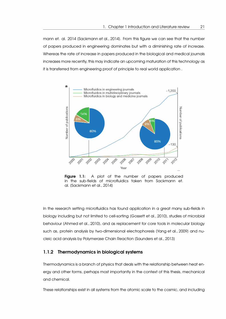
mann et. al. 2014 [Sackmann et al., 2014]. From this figure we can see that the number
of papers produced in engineering dominates but with a diminishing rate of increase.
Whereas the rate of increase in papers produced in the biological and medical journals
increases more recently, this may indicate an upcoming maturation of this technology as
it is transferred from engineering proof of principle to real world application .
Figure 1.1: A plot of the number of papers producedin the sub-fields of microfluidics taken from Sackmann et.al. [Sackmann et al., 2014]
In the research setting microfluidics has found application in a great many sub-fields in
biology including but not limited to cell-sorting [Gossett et al., 2010], studies of microbial
behaviour [Ahmed et al., 2010], and as replacement for core tools in molecular biology
such as, protein analysis by two-dimensional electrophoresis [Yang et al., 2009] and nu-
cleic acid analysis by Polymerase Chain Reaction [Saunders et al., 2013]
1.1.2 Thermodynamics in biological systems
Thermodynamics is a branch of physics that deals with the relationship between heat en-
ergy and other forms, perhaps most importantly in the context of this thesis, mechanical
and chemical.
These relationships exist in all systems from the atomic scale to the cosmic, and including
22
biological systems. There are a number of laws that have been defined in thermodynam-
ics that govern how the relationship of heat and other forms of energy exist and interact
in any system, that are universally obeyed. Firstly energy cannot be created or destroyed.
Secondly it is stated that the amount of entropy within a system, that is to say the num-
ber of available thermodynamic states, must increase as a function of time. It appears
on face value that biological systems contradict this second law as it appears that order
is preserved or in fact increased in biological systems, however, of course no biological
system can be isolated from its environment. Because natural processes utilize chemical
energy in order to preserve and increase order within that system.
From this it can be said that the basic principles of thermodynamics do indeed underlie
and govern all biological processes at some level and therefore presents the fact that
there may be many instances where we may want to measure the response of some
biological system in relation to changes in the heat of that system, or indeed to dictate
the behaviour of some biological system by manipulating the underlying thermodynamic
conditions.
Two major modes in which the thermodynamics of biological systems are measured or
manipulated are, in the measurements of protein action and stability against a temper-
ature gradient, and in the control of nucleic acid thermodynamics for amplification of
nucleic acid species for detection and sequencing. Current instrumentation or appa-
ratus for doing these measurements and manipulations, utilize sample volumes typically
in the tens of µL. The aim is to utilize a microfluidic approach to making these kinds of
measurements so that the temperatures required to perform them can be reached with
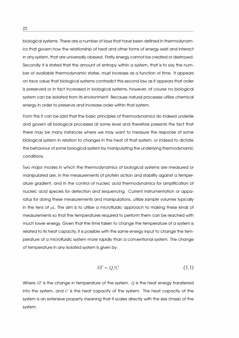
much lower energy. Given that the time taken to change the temperature of a system is
related to its heat capacity, it is possible with the same energy input to change the tem-
perature of a microfluidic system more rapidly than a conventional system. The change
of temperature in any isolated system is given by:
δT = Q/C (1.1)
Where δT is the change in temperature of the system. Q is the heat energy transferred
into the system, and C is the heat capacity of the system. The heat capacity of the
system is an extensive property meaning that it scales directly with the size (mass) of the
system.
1. Chapter 1 Introduction and Literature review 23
This fundamental principle will be leveraged throughout this thesis in an attempt to in-
crease the speed at which measurement and modulation of a biological system, can
be made, along a temperature gradient. Such that analysis of these systems can be
performed more quickly with less reagents and sample utilized, by miniaturizing the instru-
mentation into the microfluidic regime.
It should be noted that during the experiments involved in this thesis, the sample is always
either measured at room temperature or above. What this means is, that at any point
at which it is required for the sample to be cooled down, this is performed passively. In
that, heat is lost to the surrounding material, which is the air in the room containing the
measurement system.
When an object is heated to above ambient temperature, heat is always being lost to
the surrounding material. Therefore when it is required for the temperature of the sample
to be maintained at some value higher than the ambient temperature of the room, a
balance of input heating energy and natural heat loss to the surroundings must be struck.
When this balance is struck the sample can maintain a thermal equilibrium between heat
loss and heat gain, at a temperature higher than the ambient temperature.
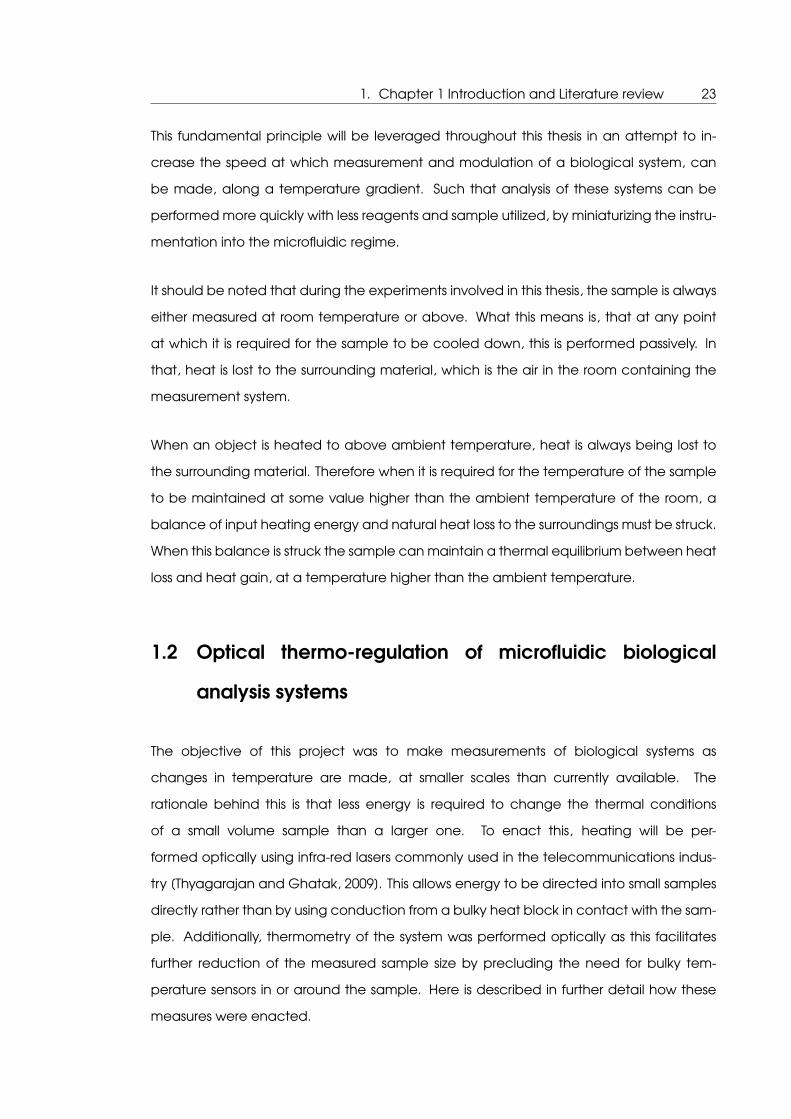
1.2 Optical thermo-regulation of microfluidic biological
analysis systems
The objective of this project was to make measurements of biological systems as
changes in temperature are made, at smaller scales than currently available. The
rationale behind this is that less energy is required to change the thermal conditions
of a small volume sample than a larger one. To enact this, heating will be per-
formed optically using infra-red lasers commonly used in the telecommunications indus-
try [Thyagarajan and Ghatak, 2009]. This allows energy to be directed into small samples
directly rather than by using conduction from a bulky heat block in contact with the sam-
ple. Additionally, thermometry of the system was performed optically as this facilitates
further reduction of the measured sample size by precluding the need for bulky tem-
perature sensors in or around the sample. Here is described in further detail how these
measures were enacted.

24
1.2.1 Lasers and Fluorescence
Lasers are a particular subset of light sources, they differ from most other sources in that
they emit a highly coherent intense beam of light. In order to produce lasing significant
differences exist when compared to the manner in which light is produced by conven-
tional light sources. In lasing, a population inversion occurs along a relatively long path
length within some kind of resonator such that optical gain is produced. Overall this pro-
cess leads to the production of an intense beam of electromagnetic radiation of a tightly
confined wavelength range, that has the additional characteristic of being much more
highly collimated than other light sources. A brief discussion of how this process occurs
will now follow.
1. Chapter 1 Introduction and Literature review 25
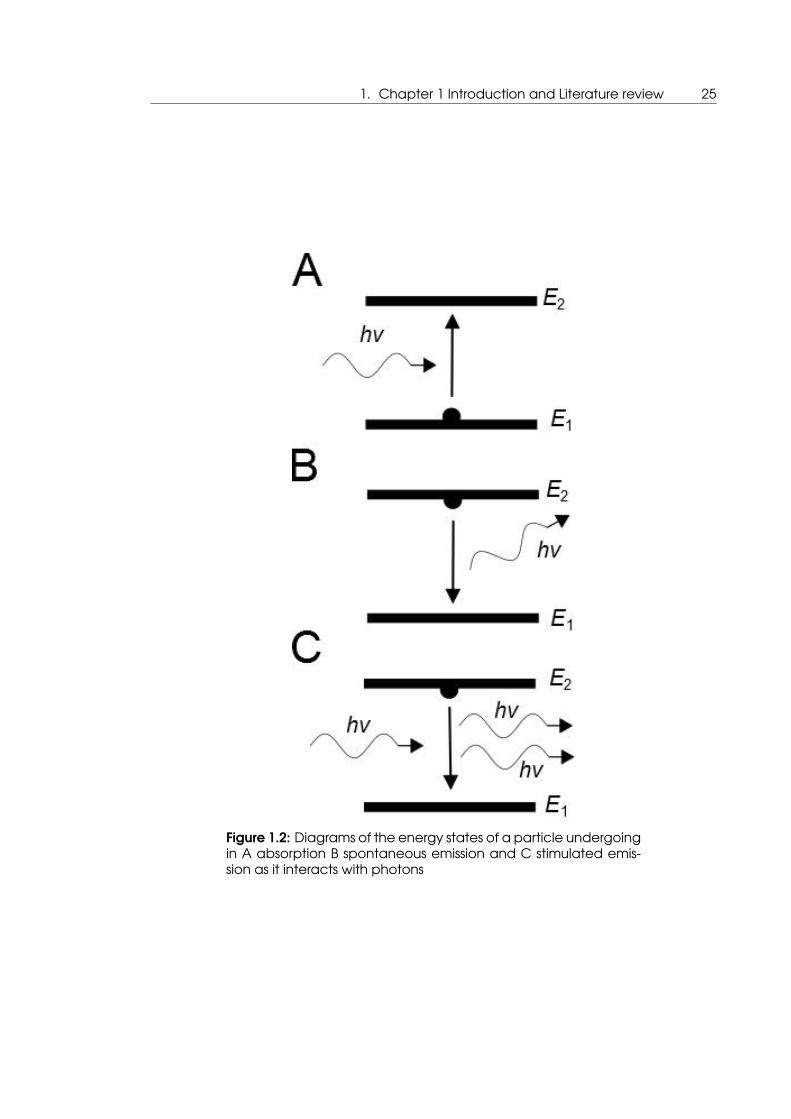
Figure 1.2: Diagrams of the energy states of a particle undergoingin A absorption B spontaneous emission and C stimulated emis-sion as it interacts with photons
26
Stimulated emission is closely related to the processes of absorption and spontaneous
emission, as well as fluorescence, which will be discussed later, these processes are illus-
trated in figure 1.2. Absorption is the process by which the energy of a wave is transferred
onto matter, here a photon interacts with an electron that forces it up into a higher en-
ergy state, or excited state E2 in figure 1.2. In spontaneous emission the excited system
subsequent to absorption will naturally decay back into the original ground state E1 in the
figure 1.2, in order to do this the photon of the difference in energy between the states
is emitted. In stimulated emission an electron in the excited state interacts with an inci-
dent photon such that both that incident photon and another are emitted in the same
direction and with the same wavelength or energy.
In order for stimulated emission to occur there must be a population inversion of avail-
able electrons within an optical gain medium situated between a resonant cavity that
is being pumped with photons from another source. In a typical laser the resonant cav-
ity is formed by two reflecting mirrors facing each other at opposing ends of the gain
medium, when the pumping source is switched on and supplying photons to the reso-
nant cavity a proportion of these electrons absorb and move into the excited state, a
proportion of these will then by spontaneous emission emit a photon along the axis of
the cavity, these photons as they are reflected back and forth in the cavity will in turn in-
teract with electrons in the gain medium moving them into the excited state. This light
along with the pumping source working together eventually move the entire system into
the state where the majority of the electrons are in the excited state, in this configuration
a population inversion is said to have occurred and the situation is primed for stimulated
emission and lasing.
Fluorescence is another property of the interaction of electromagnetic waves and mat-
ter. It is in effect very similar to the related processes of absorption and spontaneous
emission described earlier. Here an electron interacts with an incident photon and en-
ters an excited state, but the system relaxes vibrationally into a slightly lower energy level,
by the loss of energy, by phonon transfer. This means that when the system relaxes back
into the original ground state a photon is emitted at a longer wavelength, that is to say
of lower energy is emitted. Overall we can see that a high energy photon enters the sys-
tem and a lower energy photon plus the difference in heat leave the system, where the
difference in the energies of the two photons is referred to as the Stokes shift. The quan-
tum yield (Φ) is a measure of how many photons will be emitted from such a fluorescence
1. Chapter 1 Introduction and Literature review 27
system for every photon absorbed.
Φ =Number of photons emitted
Number of photons absorbed(1.2)
The property of fluorescence is exhibited by a great many naturally occurring and syn-
thesized compounds and molecules. Naturally occurring fluorescence within living things
is often termed bio-fluorescence. One key example of a bio-fluroescent molecule is the
green fluorescent protein (GFP), derived from the species Aequorea victoria, and has
found a myriad of uses in molecular biological analysis. For example it can be used as a
reporter of gene expression as when the gene is transcribed, there is an intense fluores-
cence signal. It has also been used as a readout mechanism in a variety of bio-sensors,
and indeed GFP’s fluorescence was used later in this study as a reporter of protein stabil-
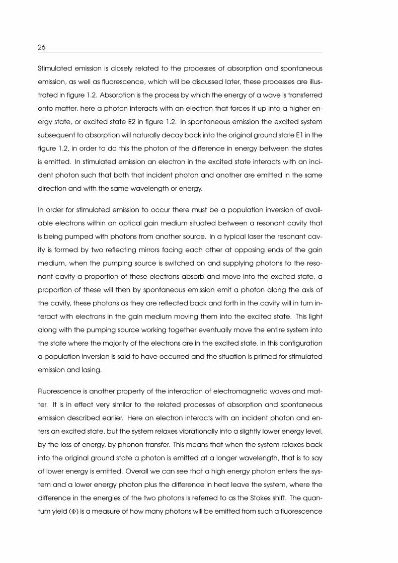
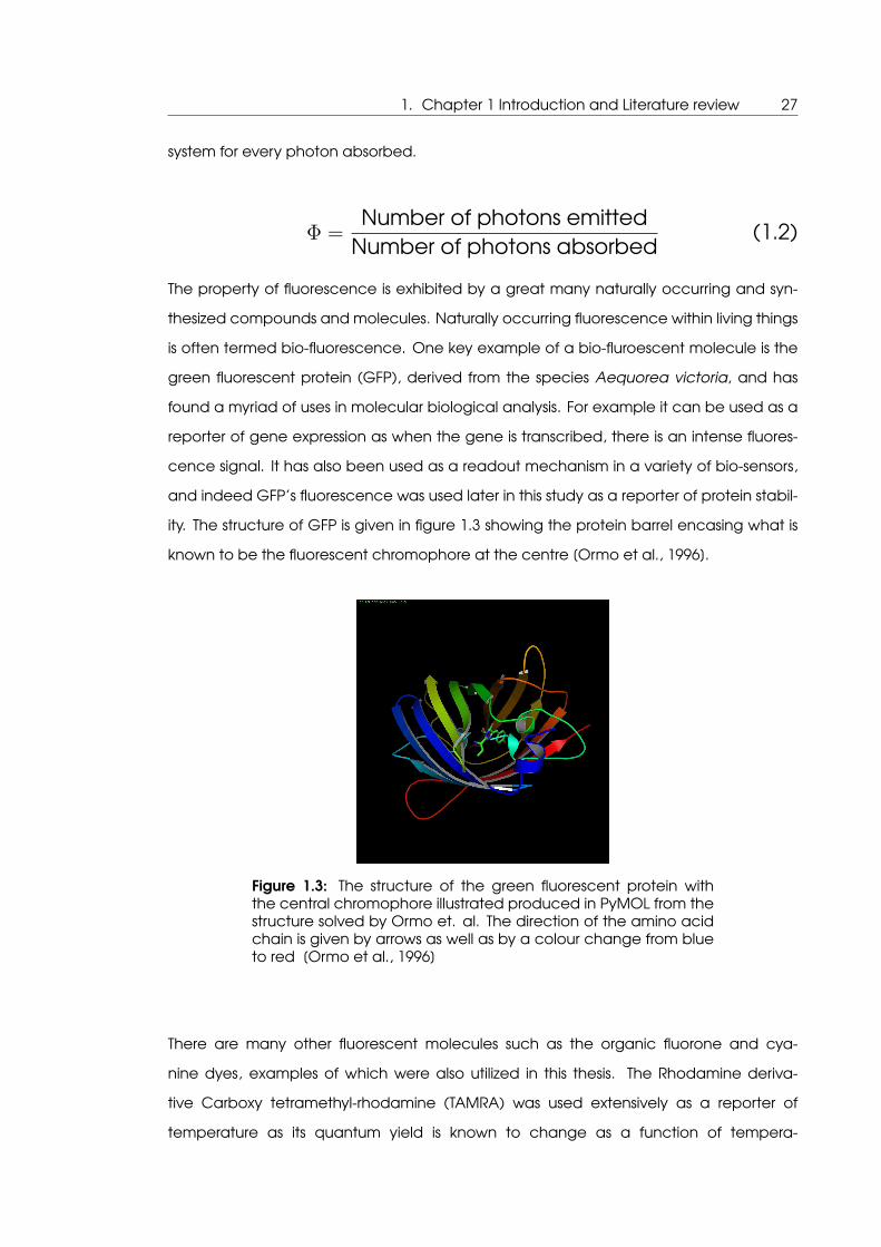
ity. The structure of GFP is given in figure 1.3 showing the protein barrel encasing what is
known to be the fluorescent chromophore at the centre [Ormo et al., 1996].
Figure 1.3: The structure of the green fluorescent protein withthe central chromophore illustrated produced in PyMOL from thestructure solved by Ormo et. al. The direction of the amino acidchain is given by arrows as well as by a colour change from blueto red [Ormo et al., 1996]
There are many other fluorescent molecules such as the organic fluorone and cya-
nine dyes, examples of which were also utilized in this thesis. The Rhodamine deriva-
tive Carboxy tetramethyl-rhodamine (TAMRA) was used extensively as a reporter of
temperature as its quantum yield is known to change as a function of tempera-

28
ture [Baaske et al., 2007], in a way that will be detailed more thoroughly in subsequent
sections. Certain DNA biding dyes such as SYBR green I is used as a reporter of DNA con-
centration throughout this thesis as its quantum yield is known to be increased when it is
bound between the two strands of a DNA molecule [Cosa et al., 2001]. The structure of
this is shown in figure 1.4 which reveals the high concentration of aromatic rings known to
be fluorescent [Guilbault, 1990].
Figure 1.4: The structure of SYBR green I by Klaus Hoffmeier re-leased to public domain
1.2.2 Optical thermometry
There are a multitude of ways in which the temperature of a sample or system can be
measured. Typically in commercial instruments where direct control of temperature is
required a feedback loop is formed. With a thermocouple used to measure the temper-
ature of the system and power then supplied accordingly to heating elements, which are
likely to be either based on joule heating or the thermoelectric effect found in some ma-
terials. In joule heating electrical power is passed through some substance that has some
electrical resistance. Here as it is known that P = I ∗ V where I and V are the current
passing across the resistative element, P the power across the element will be converted
from electrical energy to thermal energy. In the thermoelectric or Seebeck effect. A volt-
age bias across a device composed of a doped semiconductor can cause heat to be
pumped from one side to the other. In either of these scenarios the heating (or cooling)
device is thermally coupled to a sample by use of some type of mount that can be re-
ferred to as a ’heat block’. In the example of a PCR machine in which a sample must

1. Chapter 1 Introduction and Literature review 29
be heated above ambient in a controlled manner, the thermal energy of the heat block
then transfers conductively through the walls of the plastic or glass sample tube to the
sample itself. A schematic of this is represented in figure 1.5 to illustrate that the mea-
surement of temperature is not made at the sample and that the equipment required to
regulate the temperature of the sample are themselves far larger than the sample itself.
Figure 1.5: Schematic of a typical setup for heating some fluidsample for analysis. 1 is the sample, 2 is the sample container, 3is the thermocouple, 4 is the power supply to the heat regulatoryelement, 5 is the heating element itself, and 6 is the heat blockthat couples the heater to the sample container.
In either case the temperature is typically measured by a thermocouple that is located
close to the sample and the temperature of the sample is inferred and assumed to nor-
malize to the measured temperature (likely that of the heat block). As the surrounding
heat block has a large capacity for the storage of thermal energy, the laws of thermo-
dynamics dictate that the entire system must reach a thermal equilibrium given enough
time and that time will be sufficiently short if the heat block is a large enough sink of ther-
mal energy.
The use of thermocouples in microfluidic systems poses a geometrical problem in that (at
the time of this research) even the smallest thermocouples are of similar size to that of any
sample container that could be considered microfluidic (80µM as produced by Okazaki
Manufacturing Company). This means that a thermocouple measuring the tempera-
ture of a microfluidic system would potentially be one of the more massive elements of
that system, implying that any fluid channels would have to be designed to be sufficiently

30
large so that they were not occluded by the thermocouple, and that the thermodynamic
behaviour of the entire system was not dominated by the presence of the thermocouple
itself with its relatively large ability to store thermal energy. A schematic of this is repre-
sented in figure 1.5 to illustrate that the measurement of temperature is not made at the
sample and that the equipment required to regulate the temperature of the sample are
themselves necessarily far larger than the sample itself.
in order to circumvent this difficulty in mounting a bulky temperature probe in or around a
sample in a microfluidic setting a number of approaches have been adopted by different
research groups. A short review of these will now ensues.
One design philosophy that can be adopted is to utilize techniques adopted from the
semiconductor industry to build a microfluidic device that has miniaturized heating and
temperature measurement systems embedded. These may take the form of fully embed-
ded bespoke systems [Hsieh et al., 2008], or microscale commercially available systems
embedded in a polymer chip [Maltezos et al., 2008]. Any implementation of this design
philosophy would likely mean that the embedded thermal sensors, being that they are
embedded near the sample holder must be disposed of once the chip has been used.
This contravenes the manner in which biological analysis systems are used in the real
world where once a sample has been analyzed only the inexpensive plastic or glass con-
tainer of the sample is disposed of, which keeps the overall cost of performing many
analyses over time down. Another disadvantage would be that the thermocouple will
be located distally from the sample itself, so there could be assumed to be some off-
set between the measurement and the true temperature of the sample. Perhaps the
principal advantage of this approach is that the temperature measurement at the ther-
mocouple can be assumed to be well calibrated and precise assuming the device has
not undergone a catastrophic failure, which would be obvious if it occurred.
There are, however, a number of non-contact methods in which the temperature of a
sample may be ascertained. These methods impart the advantage that the relatively
expensive temperature sensing elements can be separate from the sample container,
driving the cost of any derived device down.
The simplest methodology for implementing non-contact thermometry would be to use
an off-the-shelf infra-red imaging system. The use of infra-red imaging systems has prolif-
erated in general terms as they are used as the forward looking infra-red (FLIR) detection
systems in a wide range of military settings. Although the proliferation of this type of tech-
1. Chapter 1 Introduction and Literature review 31
nology has without doubt driven the cost of such systems down, it would also be fair to
say that as of the time of writing such a system is still prohibitively expensive with costs
of around £1000. It can be said that the use of a drop in solution such as this would
present the fewest engineering challenges, but could probably be considered unfeasi-
ble for use in any commercial detection system that required thermometry of a sample.
There is, however, a wealth of research papers when this is the solution of choice for per-
forming thermometry of a microfluidic system [Ravey et al., 2012]. Another complexity of
using such a setup to measure the temperature of the system is that if an infra-red heat-
ing source such as a laser is used to heat the sample then this could potentially interfere
with or damage the sensor of the FLIR sensing device [Hawkins, ].
Another method that has been used to perform thermometry in microfluidic systems is to
use Raman spectroscopy [Kim et al., 2006], as the Raman spectra of water (in which one
is likely to make measurement of some biological entity) is known to be temperature de-
pendent [Smith et al., 2005]. This approach would have the advantage over using an FLIR
device in that the measurement system can be constructed from parts more commonly
associated with optics laboratories such as lasers and photo multiplier tubes, rather than
using a sealed bespoke measurement system. Raman spectographic thermometry of
water would have the inherent advantage when compared to several methods evalu-
ated later on in this section in that the measurement is made of the water itself, meaning
that no other substances are added to the buffer of the biological entity under study. This
means that experimental reagent mixture concentrations could be directly ported from
any other larger volume reaction with no modification. The chief disadvantage of the
use of any Raman spectographic approach is the low signal to noise ratio, as the Raman
effect is weak [Alfano and Ockman, 1968], which necessitates highly sensitive detection
systems such as an avalanche photo multiplier tubes which will require very careful shield-
ing from any background light. Whilst this isn’t of course impossible to achieve, it is in itself
an engineering challenge. Additionally changes to the buffering conditions such as salt
concentration or pH would affect the Raman spectra
Yet another method in which the temperature of a sample can be measured in a non
contact manner, is to use the change in refractive index of materials as a function of
temperature. In this kind of setup a laser is directed at an angle to a liquid sample that is
in interface with a high quality glass window this beam is reflected into a photodiode. The
reflectivity of light at this water-glass interface changes as a function of temperature, the

32
change in temperature of the fluid can then be calculated if the reflectivity coefficients
of the water and glass are well characterized. The advantages of this kind of system are
that it can, if set up correctly, gives very high thermal resolution. The chief disadvantages
seem to be that the measured temperature range is small [Baffou et al., 2012] and that
the thermoreflectance coefficient must be well characterized for any material used in
the setup [Fan and Longtin, 2000].
All the previously mentioned methods for performing thermometry at the microscale
make direct measurements of some property of the buffer (likely mostly water in this sce-
nario). However, there are also a number of methods that employ some additive to the
buffer that has a property, which changes as a function of temperature, is then read
off to perform thermometry of the containing buffer. This methodology typically has the
advantages that the signal to noise ratio of the property being read out would tend to
be larger than other previously discussed methods, for example Raman spectroscopy,
and that the property being read is typically fluorescence intensity meaning the read-
out equipment can be as simple as an excitation source and a photodiode. The prin-
ciple disadvantage is that there may be no way to tell, apart from experimentation,
what effect adding something to the buffer will have on any biological reaction occur-
ring in the microfluidic device. It is well characterized, for example, that PCR efficiency
is affected by buffering conditions to a large degree and sometimes in a complex man-
ner [Schrader et al., 2012]. It is likely that there could be an inverse relationship between
these stated principal advantages and disadvantages, in that the signal to noise ratio de-
rived from some temperature-sensitive additive will likely to be concentration-dependent,
which is also likely to be true of any effect in disrupting the buffering conditions of some
reaction.
One such additive that could be used for remote thermometry are encapsulated liquid
crystals, often described as thermochromic pigments, these are commonly seen in nov-
elty products such as colour changing beverage mugs and the like. Whilst the exact for-
mulation of any of these pigments may not be fully disclosed by the manufacturers, they
are widely and cheaply available. An example of the range of thermochromic paints
available commercially from a single manufacturer is shown in figure 1.6. Here the colour
reflected, that being the visible colour, of the thermochromic pigment changes quite dra-
matically at some transition temperature [Christie and Bryant, 2005]. These sharp colour
transitions of liquid crystal thermochromics may mean that they are unsuitable for mea-

1. Chapter 1 Introduction and Literature review 33
suring a biological reaction that takes place over a wide temperature range such as PCR.
However, this can potentially be overcome by using combinations of different liquid crys-
tal thermochromics that have transitions at key temperatures you would like to monitor a
reaction at. In the example of PCR this may be 95◦C and 60◦C [Hoang et al., 2008].
Figure 1.6: A guide to the range of commercially available ther-mochromic pigments from a single manufacturer. used by per-mission Indestructible Paints Ltd.
The use of thermochromic pigments to measure temperature bears one similarity to ther-
moreflectance in that the signal being measured is of the reflected light. The remainder
of the additives that can be used to gauge the temperature of a sample differ in that
they function instead by emitting light themselves, most commonly as a fluorescent sig-
nal by spontaneous emission as detailed earlier. Different classes of such additives con-
sidered for use in thermometry in biologically compatible microfluidics are organic dyes,
polymers, quantum dots, nano-diamonds and lanthanide based complexes
Lanthanide based nano-particles have been shown to be used as thermometers as mi-
croscales in multiple examples [Brites et al., 2011] including even thermometry inside a
living cell [Kucsko et al., 2013]. The fluorescence in most of these examples are con-
veniently excited by relatively cheap sources such as LEDs or common wavelength
lasers, and they have an intrinsic advantage in that they are not subject to the effect
of irreversible photobleaching , as they cannot undergo the oxidation that causes this
[Yu et al., 2014]. One disadvantage that could be suggested for the use of these ma-
terials is that they are currently quite exotic and have a complicated synthesis proce-
dure [Zhang et al., 2010].
34
Quantum dots are nanocrystals of semiconductor material that exhibit a band gap that
is tunable as a function of their size [Alivisatos, 1996]. This band gap will result in a flu-
orescence that has been shown to be temperature dependent. Much like Lanthanide
based nanoparticles, due to their inorganic nature they cannot undergo light induced
chemical change resulting in irreversible photobleaching, which could be an advantage
in their use as a thermometry method. However, they are prone to aggregation which
although it can be overcome by the use of functionalization with streptavidin, this func-
tionalization will not survive beyond the denaturation temperature of that protein and
therefore could not be used as a temperature probe in a high temperature biological
microfluidic system such as a PCR device [Li et al., 2007].
Nanodiamonds with nitrogen vacancy centres have also been used as probes of temper-
ature at the nanoscale, this is achieved by measuring the electron spin resonance of the
electrons composing the nitrogen vacancy centre [Neumann et al., 2013]. This technique
would seem to lend itself well to the measuring of biological processes in microfluidic de-
vices as it operates well over the temperature range at which key biological reactions
occur, and would not be subject to any effects such as irreversible photobleaching. Ad-
ditionally as nanodiamond is highly inert it would potentially be highly bio-compatible. To
illustrate this, the technique has been used to perform thermometry non-invasively in liv-
ing cells [Kucsko et al., 2013]. The principal drawback in using this methodology is that a
complex spin resonance measurement system must be constructed around the sample.
There are also a large number of aromatic hydrocarbon compounds that can be used
for non-contact thermometry. These are normally used in a regime where the compound
is fluorescent and the intensity, lifetime, or spectrum of this fluorescence changes in some
way as a function of temperature. A large number of these are discussed in a recent
review by Palacio & Carlos [Brites et al., 2012] cf. table 2. A Large majority of these are
not suitable for performing thermometry of biological systems in microfluidic devices as
they do not operate over the temperature range at which one might want to monitor a
biological process, that being the temperature range of the liquid phase of water.
Typically these temperature sensitive dyes are small molecular weight hydrocarbons but a
number of more complex molecular temperature probes have been made by the linking
of organic dyes to polymer molecules [Hu and Liu, 2010]
The mechanism by which the fluorescent intensity of such an organic dye is altered by
a change in temperature will now be briefly detailed. What essentially occurs is that the

1. Chapter 1 Introduction and Literature review 35
quantum yield, which is the ratio of emitted photons to incident excitation photons in a
fluorescent process, becomes decreased, in a way described by the following scheme.
The kinetics of the quantum yield of a fluorophore are given in equations 1.3 & 1.4
F + hνE −→ F ∗kf−→ F + hνF
↓ ki
F
(1.3)
Where F is a fluorophore in the ground state, F ∗ is a fluorophore in the excited state, hνE
is an excitation photon, hνF is a fluorescence photon, kf is the rate of radiative processes
& ki is the rate of non-radiative processes.
φF =kf
kf + ki(1.4)
Where φF is the quantum yield of fluorescence, kf is the rate of radiative processes, and
ki is the rate of non-radiative processes.
The rate kf being the rate of radiative processes, is really the rate of emission of photons
from fluorescence, whereas the rate of non-radiative processes ki includes the rate con-
stant for all thermally activated processes. It must be, therefore, that the quantum yield
of a fluorescent process will decrease as a function of temperature.
Additionally the temperature of the solvent will also affect the quantum yield of any fluo-
rophore in solution in a more complex manner. The combination of these two processes
is that most fluorophores will exhibit a decrease in quantum yield for an increase in tem-
perature [Lou et al., 1999]
Rhodamine B is one such organic dye that along with its derivatives are known to exhibit
a temperature dependence to their fluorescence with a range of operation that covers
the scope of biological processes. Indeed this was the system that was used to do non-
contact thermometry of biological entities in microfluidic systems during the experiments
described in this thesis.
Rhodamine B and its derivatives exhibit strong fluorescence signals as they have three

36
benzene rings in a row, which has been shown to be the most fluorescent configuration
of aromatic hydrocarbons [Guilbault, 1990]. This strongly fluorescent three carbon ring
structure is illustrated for the molecule TAMRA is shown in figure 1.7.
Figure 1.7: The structure of the TAMRA moleculefrom National Center for Biotechnology Informa-tion. PubChem Compound Database; CID=2762606,http://pubchem.ncbi.nlm.nih.gov/compound/2762606 (ac-cessed May 20, 2015).
The backbone structure of organic dyes such as TAMRA exhibits fluorescence as the
double-single carbon bonds terminated with R groups at either end form a constrained
system (displayed at the top of figure 1.7 then represented at the bottom of figure 1.8).
A π electron in this system will have a finite number of solutions for the Schrödinger equa-
tion with different energies that photons of the same energies can interact with. Once a
photon is absorbed by the system at one of these energy levels, the entire system enters
an excited state at a higher energy. Eventually the system will relax back into the ground
state by the release of a fluorescence photon, however, in the meantime smaller energy
losses occur due to rotational and vibrational modes that have a shorter lifetime. There-
fore the photon released has a lower energy (longer wavelength) than the absorbed.
This is what causes Stokes shift in fluorescence.
1. Chapter 1 Introduction and Literature review 37
Figure 1.8: Diagram of the potential well particle in a box modelfor a conjugate system of a fluorescent dye. The vertical axis isenergy, the horizontal axis is the length of the constrained system.C are the elements of the conjugate system in which the π elec-trons are free to move within. R are the groups next to the con-jugate system in which electrons from that system are forbiddenfrom moving into. 1, 2 & 3 are the three solutions for Schrödinger’sequation that can exist within the system with associated higherenergy rotational & vibrational modes. hνE is an excitation pho-ton that causes the transition to an excited state, where E is thattransition. V1 is a vibrational or rotational transition. R is a re-laxation back into a rotational or vibrational mode surroundingthe lower energy state. V2 is a vibrational or rotational transitionback to the lowest vibrational or rotational state. hνF is a fluo-rescence photon of lower energy than hνE where the differencein energy is equal to the sum of the energies of the two vibra-tional or rotational transitions. The vibrational or rotational transi-tions V1 & V2 occur as these processes are relatively fast. This figurewas adapted from Handbook of fluorescence spectroscopy andimaging: from ensemble to single molecules [Sauer et al., 2010]
38
A history of the use of Rhodamine B and its derivative TAMRA and why this is the optical
thermometry method of choice, for this thesis, will now be given
The temperature dependence of the fluorescence intensity of Rhodamine B was first es-
tablished in their use in a dye based laser system in which the gain medium of those
systems was Rhodamine B, where the system would fall in performance as the gain
medium heated up through the processes outlined earlier [Gallery et al., 1994](original
paper unseen [Drexhage, 1973]). Initially this temperature-dependent fluorescence
was exploited to remotely measure the temperature of surfaces [Gallery et al., 1994,
Romano et al., 1989]. Rhodamine B would then go to be used to measure the tempera-
ture of flowing systems at the macro-scale [Sakakibara et al., 1993] and then at the mi-
croscale [Ross et al., 2001, Shah et al., 2009]. The fluorescence intensity (quantum yield)
of the rhodamine B derivative TAMRA was shown to be temperature-dependent, in line
with previous measurements by others and the spectrum in terms of wavelength distribu-
tion was also shown to be temperature independent in line with previous measurements,
meaning that it can be described using the scheme laid out in equations 1.3 & 1.4.
The use of the Rhodamine B derivative TAMRA as a temperature probe had the following
advantages over the other methods for doing non contact thermometry that were previ-
ously mentioned, leading to it being the preferred method for performing this procedure:
• The chemical itself is relatively cheap
• in order to measure the relative fluorescence to gauge temperature, the detection
system could be as theoretically simple as a photodiode and an optical filter (i.e. a
piece of coloured glass)
• the quantum yield of TAMRA is known to have a large change in the domain of
temperature at which one would seek to measure changes in a biological system,
that being between ambient and 100◦C[Kemnitz et al., 1989]
• it was an experimental result of this work, that although TAMRA did inhibit PCR in a
concentration dependent manner, this was not catastrophic as PCR could still be
performed with high concentrations (i.e. visible to the naked eye) of TAMRA present
• TAMRA can be excited to fluoresce using green light, which is widely available as
Nd:YAG lasers frequency doubled to emit at 532nm are commonly installed in con-
focal microscope systems, as well as being a common filter ’channel’ installed on
fluorescence microscope setups. As well as generally
1. Chapter 1 Introduction and Literature review 39
1.2.3 Closed loop Optical heating by infra-red laser with PID control
In the most basic case, the fluorescence of TAMRA can be used to calculate the temper-
ature of the sample or a point in the sample from a microscope image for later analysis.
However in some cases, such as in a microfluidic PCR type device, the sample must be
moved to certain set temperatures in a pattern over the timescale of up to an hour.
In order to achieve this, feedback between the temperature measurement, in this case
optical thermometry by the measurement of the fluorescence of TAMRA and the heating
mechanism, in this case an infra red laser, must be established.
The most commonly employed feedback mechanism used throughout the world is the
proportional integrative derivative controller (PID control). with up to 97% of the con-
trollers in place in industry utilizing this method of control [Aström and Murray, 2010]. In the
simplest sense PID controllers take an input value from the measurement system (known
as the Process Variable) and compare this to a Set Point at which the system is supposed
to be measuring to give the Error. An output is then made to something connected to
the system to attempt to minimize this error, this is the controller output. A generalized
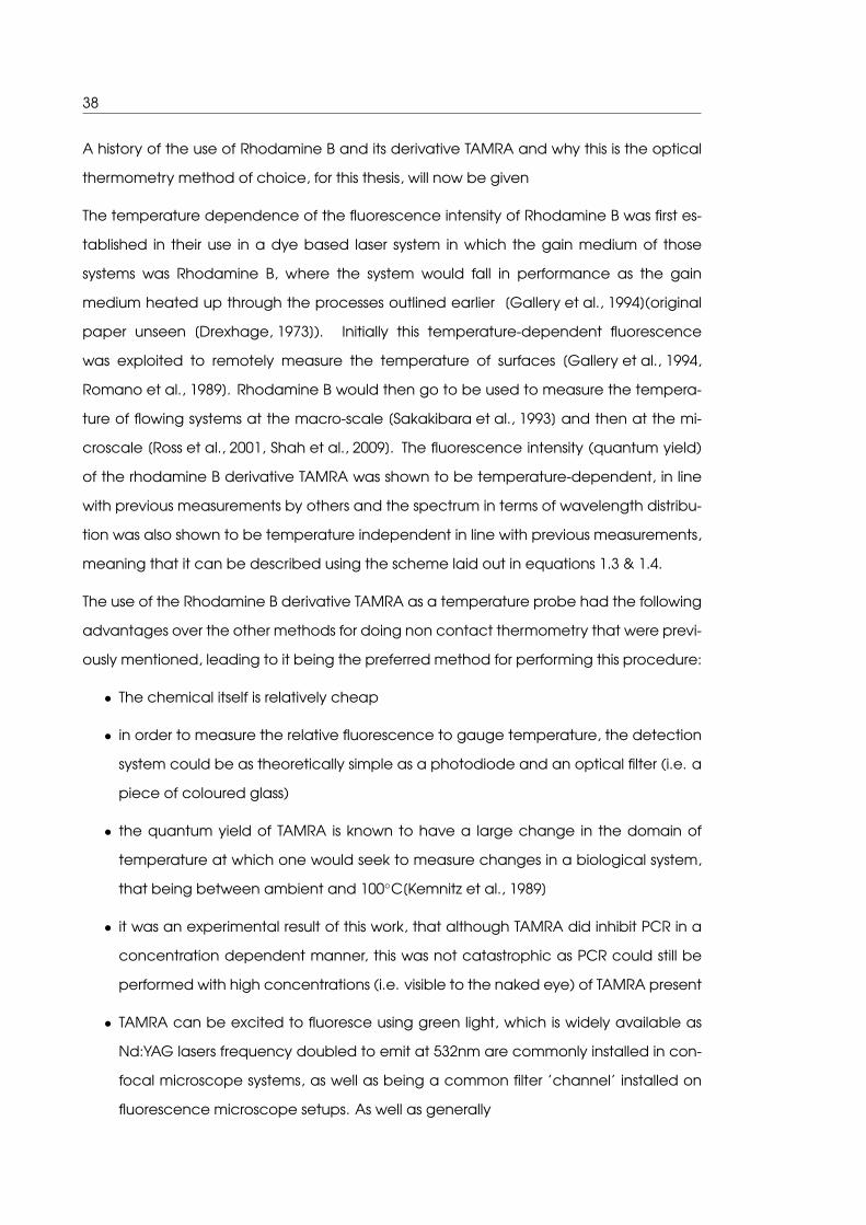
schematic of a typical PID control loop is given in figure 1.9
Figure 1.9: A graphical representation of a typical PID controlloop
The PID control loop has three terms represented on figure 1.9, these are the Proportional,
Integral and Derivative, that are used to calculate the Controller output, these terms will
now be stated mathematically.
The proportional term is the simplest of the three terms in a PID control loop it is given by:

40
Pout = Kp e(t) (1.5)
Where Pout is the contribution of the proportional term to the controller output Kp is the
proportional gain parameter and e(t) is the current error between the set point and the
process variable. The value of the proportional gain parameter is specific to any system
and can be tuned such that the behaviour of the system in terms of how close to a set
point the system will stabilize at, how quickly it will move between set-points, and how
much overshoot is likely to occur can be regulated. This tuning of the proportional gain
parameter can be deduced by experimentation.
The Integral term is the integral of the error since the control loop was initiated given by:
Iout = Ki
∫ t
0
e(τ) dτ (1.6)
Where Iout is the contribution to the controller output of the integral term. Ki is the integral
gain parameter, all things stated about the proportional gain parameter also apply to the
integral gain parameter. And∫ t0e(τ) dτ is the integral of the error evaluated from the time
the control loop started until the present time. The integral term will function to offset any
droop that the proportional term would have if implemented on its own
The Derivative term is, given by:
Dout = Kdd
dte(t) (1.7)
Where Dout is the contribution of the Derivative term to the controller output, Kd is the
proportional gain parameter, as before everything that must be considered for the other
two gain constants should also be considered here, and ddte(t) is the derivative of the
error at the current time. As the derivative of the error at any one time is essentially the
current trajectory of the system, the derivative term assists the system in settling in on a
final value, avoiding jitter and fluctuations.
Taking these three terms together we can state the equation in its final form
1. Chapter 1 Introduction and Literature review 41
u(t) = Kpe(t) +Ki
∫ t
0
e(τ) dτ +Kdd
dte(t) (1.8)
Where u(t) is now the total controller output.
All tuning of gain parameters in this thesis were performed manually, and the components
of the system were as follows:
• the controller output is the power supplied to the infrared lasers
• the set point is the temperature value of some PCR thermocycling program
• the process variable is the temperature as recorded by optical thermometry using
the fluorescence of TAMRA
1.2.4 Fluorescence signal extraction by use of lock-in amplifiers
One of the principle drawbacks of using TAMRA fluorescence as method of performing
optical thermometry is that irreversible photobleaching will occur. The process of irre-
versible photobleaching of fluorescent dyes has been known of for a long time. It occurs
due to photon interactions which are necessary to put the fluorophore in the excited
state but in a minority of cases induce chemical modification such that the molecule is
no longer capable of being fluorescent [Livinson, 1949].
This photobleaching effect is a well known problem in the use of fluorescent dyes in mi-
croscopy work where cellular components are fluorescently labelled and may be ob-
served for some time, in that the microscope images will become dimmer until the point
where the cellular components are no longer resolvable due to the loss of fluorescent
dyes capable of fluorescing [Bernas et al., 2004].
This photobleaching effect could also prove to be problematic where the temperature
dependence of a fluorescent dye is used to perform optical thermometry. When using
the temperature dependence of TAMRA to perform optical thermometry the fluorescent
reading is compared relative to some reading that was taken previously. This is then com-
pared to a calibration function measured previously of what the relative fluorescence
will be at some higher temperature. However in the presence of photobleaching the
amount of molecules capable of contributing to this fluorescence is decreased meaning
that for the same illumination the fluorescence will be decreased.

42
In this scenario an optical thermometry measurement at constant temperature made
with a constant influx of photons will appear to become darker, and therefore hotter
over time. This could prove to be catastrophic when the optical thermometry method is
used to regulate the temperature of some fairly long lived process (such as PCR)
It is known that the rate of photobleaching increases as a function of the amount of
incident photons [Eggeling et al., 1998]. Indeed, comments have been made of previous
work using organic dyes as remote temperature probes, that they have been excellent
in their use of restricting the amount of incident photons by the use of precise shuttering
of the excitation light [Yue and Wang, 2012].
By decreasing the amount of incident photons, the amount of emmitted fluorescent pho-
tons will accordingly also decrease; if you assume the amount of background light and
noise in any detection system stays the same then the signal to noise ratio of the mea-
surement will also accordingly decrease. Within the context of using this measurement
as a method of thermo-regulation, the system will tend towards becoming increasingly
thermally unstable.
A method that can be employed to increase the signal to noise ratio of a measurement
is by the use of lock-in amplification, which will now be described. The basic layout of a
lock-in amplifier used to measure fluorescence is set out in figure 1.10
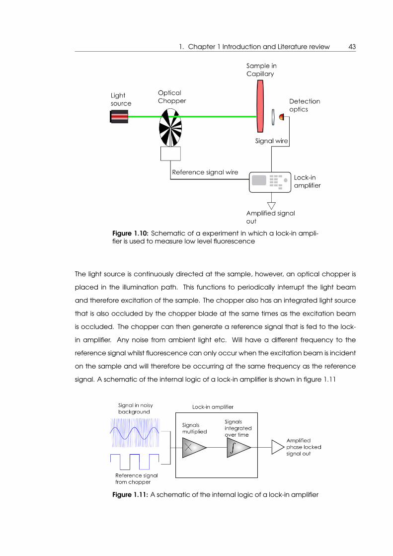
1. Chapter 1 Introduction and Literature review 43
Figure 1.10: Schematic of a experiment in which a lock-in ampli-fier is used to measure low level fluorescence
The light source is continuously directed at the sample, however, an optical chopper is
placed in the illumination path. This functions to periodically interrupt the light beam
and therefore excitation of the sample. The chopper also has an integrated light source
that is also occluded by the chopper blade at the same times as the excitation beam
is occluded. The chopper can then generate a reference signal that is fed to the lock-
in amplifier. Any noise from ambient light etc. Will have a different frequency to the
reference signal whilst fluorescence can only occur when the excitation beam is incident
on the sample and will therefore be occurring at the same frequency as the reference
signal. A schematic of the internal logic of a lock-in amplifier is shown in figure 1.11
Figure 1.11: A schematic of the internal logic of a lock-in amplifier

44
The working principle underlying the lock-in amplifier is that when sine waves (the square
wave generated by the chopper is assumed to be a sine wave for the purpose of this
example) of dissimilar frequency are multiplied a more complex oscillatory function cen-
tred around amplitude zero is the product. However when these functions have the same
frequency the product always has a positive amplitude. When an integral of these two
examples is taken which is far longer than the period of the input functions, the result is
in the case where the input functions were of different frequencies, close to zero, and
when they were of the same frequency, some value larger than zero. In this manner the
frequency of interest can be isolated and then amplified, whereas signals at all other
frequencies are filtered out.
The uses of such a system when attempting to use fluorescence as a method of optical
thermometry and avoid photobleaching, are as follows. The use of the optical chopper
immediately cuts down the number of incident photons striking the sample and therefore
accordingly decreases the rate of photobleaching. The use of the lock-in amplifier means
that the signal to noise ratio of the measurement is vastly increased, so that far weaker
fluorescence signals can be used to monitor and control the temperature, which in turn
means that for a sample with the same number of fluorophores a far weaker level of
excitation can be used which cuts down the number of incident photons and therefore
the rate of photobleaching.
1.3 Measurements of protein stability versus temperature
Proteins are a major component of all biological systems, second only to water by mass,
and representing typically around 15% in a bacterial cell [education, 2010] and 20% of
the human body [Freitas, 1998]. Proteins were first isolated by Foucroy towards the end
of the eighteenth century [Osborne, 1919], and have been major components of biolog-
ical research to date . Proteins not only are utilized as structural components by nature,
they are also the principal active components that facilitates the dynamics of processes
in biological life [Fersht, 1999], when they have an activity such as this they are termed
enzymes. Because of the fundamental nature of proteins in regulating the activity of
biological processes they are also the key targets of medical research, with in fact prac-
tically all targets in drug discovery being proteins, creating a research environment on
which some $50 billion is spent annually [Overington et al., 2006]. Furthermore the abil-
ity of enzymes to catalyze biological processes means they are utilized in a great many
1. Chapter 1 Introduction and Literature review 45
industrial processes for the production of useful products, in the food and animal feed
industry as well as in the production of chemicals industrially [Kirk et al., 2002]
1.3.1 Protein structure and stability over temperature
Proteins are formed of chains of amino acids, these are polymerized by the ribo-
some [White and von Heijne, 2004] in a specific sequence as dictated by an RNA tran-
script. Proteins are formed linearly in this way but take on complex 3d structures that also
dictate any enzymatic activity or binding function that they may have.
These amino acids are joined by the ribosome (itself a large enzymatic protein com-
plex) [White and von Heijne, 2004] by the carboxyl group of one amino acid to the amino
group of the next, this bond referred to as the amide bond forms an un-branched
polypeptide chain. A number of disulphide bridges may also exist between Cysteine
residues in this polypeptide chain that assist in holding the chain in its 3d structure. Over-
all, however, the 3d structure of a protein is dictated by thermodynamic considerations. In
that the order of amino acids in the polypeptide chain will create areas with differing lev-
els of hydrophobicity, this will cause different sections to either be more buried in the core
of the protein whilst others will tend to interact more with the water solvent the protein
evolved suspended in. From this we can say that the 3d structure and activity of the pro-
tein is genetically encoded in the corresponding DNA sequence [Anfinsen et al., 1973],
that in turn encodes the protein’s amino acid sequence.
Since an enzyme has a specific sequence it also has a specific structure as laid out pre-
viously. Moreover we can say that as this enzyme has evolved this structure over time in
a specific environment it also has a specific catalytic action related to this specific se-
quence via this structure. The 3d structure of a catalytic enzyme dictates how strongly it
can bind a substrate, additionally this structure on binding of the substrate can flex into
a configuration that more strongly favours the production of the reaction products by al-
tering the bond structure of the reaction substrates. As we have seen, the folding of an
amino acid chain into the 3d structure that dictates this enzymatic activity is governed
by thermodynamic processes, we can also say that changes in the underlying thermo-
dynamics may also alter this 3d structure and therefore this enzymatic activity, something
which has been well characterized [Wang et al., 2004].

46
1.3.2 Relevance of measurement of protein stability
It has been illustrated how proteins are of key importance to biological processes, and
because of that are of great interest from both a research and industrial perspective.
Additionally it has been shown how the structure of a protein and any enzymatic activity
it has are related to its structure and therefore the thermodynamics of the system of the
protein molecule and its environment. It therefore follows that it would be of interest to
study the structural stability of proteins as a function of temperature, and indeed this is an
area that has been studied in detail [Robertson and Murphy, 1997]. What follows is a brief
analysis of various reasons why and how measurements of protein stability with respect to
temperature are made.
The manner in which the rational development of medicine occurs is often referred to as
the drug development pipeline. This is a step-wise process with the following components:
Genetic studies such as genome wide association studies are performed to ascertain
genes and therefore protein targets that are produced from those genes. A large num-
ber of drug candidates[Sanseau et al., 2012] that may interact with these protein tar-
gets are produced. A high throughput screen of binding interaction between these
libraries is performed[Hughes et al., 2011], where a high degree of binding is said to in-
dicate that the drug candidate could be a strong inhibitor of that protein target. In-
vitro analyses are performed to ascertain if this strong inhibition leads to some positive
outcome in a cellular disease model[Hughes et al., 2011]. Experiments with the drug
candidate in animal systems are performed to check if any effects thought to be ben-
eficial to some disease-relevant condition in the cell translate to a beneficial effect
in a living animal[Hansen and Khanna, 2004]. Clinical trials are performed to verify if
any positive therapeutic effect of the drug candidate can be measured in affected
patients[Sackett and Cook, 1994].
One method of operating the component of this pipeline in which a high throughput
screen of the strength of binding interaction between drug targets and candidate drugs
is made, is to perform measurement of the stability of the protein ligand (drug candidate)
complex. It has been known for some time that the melting temperature of a protein is
affected when a ligand is bound to it in a complex [Brandts and Lin, 1990]and indeed
that the melting temperature of the complex is always therefore higher than the protein
on its own [Waldron and Murphy, 2003]. Previously measurements of the change in melt-

1. Chapter 1 Introduction and Literature review 47
ing temperature of a protein when bound to a ligand were made using the differential
scanning calorimetry technique. One disadvantage of differential scanning calorime-
try is that the heat flux into the sample must be measured extremely accurately, this can
lead to low signal to noise ratio. One method to circumvent this is to use differential scan-
ning fluorimetry, where the fluorescence of a dye with affinity for hydrophobic parts of the
protein, is measured, and increases as the protein unfolds [Niesen et al., 2007].
In experiments leading up to those detailed in this thesis, methods were developed
for performing differential scanning fluorimetry measurements by using the intrinsic flu-
orescence of certain amino acids such as Tryptophan, as it is known that the quan-
tum yield of the aromatic intrinsically fluorescent amino acids changes as denatu-
ration occurs [Lakowicz, 2007]. Initially this was performed in a microwell plate for-
mat [Aucamp et al., 2005] and was then adapted such that a microfluidic form factor
was utilized and the difference in binding strength of a protein target and a drug in the
presence of a disease associated mutation could be detected [Gaudet et al., 2010]. This
is precisely the kind of measurement that is made in the initial phase of a drug develop-
ment pipeline.
Figure 1.12: Classical and current methodology for pro-ducing enzymes for industrial processes taken from kirk2002 [Kirk et al., 2002]
Measurements of protein stability are also key to optimization of industrial processes in-
volving the use of enzymes to produce valuable products. As shown in the figure 1.12 from
48
from Kirk 2002 [Kirk et al., 2002]. In traditional biochemical engineering the diversity exist-
ing in nature was used in fermentation processes to produce valuable products. More
recently techniques have been developed such that ’directed evolution’ can be en-
acted. Here processes such as error prone PCR are used to generate artificial diversity in
the enzyme[Cirino et al., 2003], which is then tested in small batches to ascertain if an im-
provement has been made i.e. more of a product or a more specifically required product
has been produced. From a thermodynamic viewpoint the more energy a bio-reactor
has available, the faster the enzymatic process will occur. This however must be balanced
against the stability of the enzyme as has already been shown lack of stability leads to
a drop in the specific function of a protein[Shoichet et al., 1995], which in this case is the
production of an economically valuable product. For this reason measurements of pro-
tein stability are key to the cycle of optimization of some bio-catalyzed industrial process,
as shown in figure 1.13 taken from Schmid 2001 [Schmid et al., 2001], where stability mea-
surements are shown to be a key component of this cycle. Indeed previous experiments
leading up to those detailed in this thesis were concentrated on the measurement of
intrinsic protein fluorescence for the optimization of some industrial process-relevant en-
zyme, using traditional fluorimetry instrumentation [Aucamp et al., 2008].
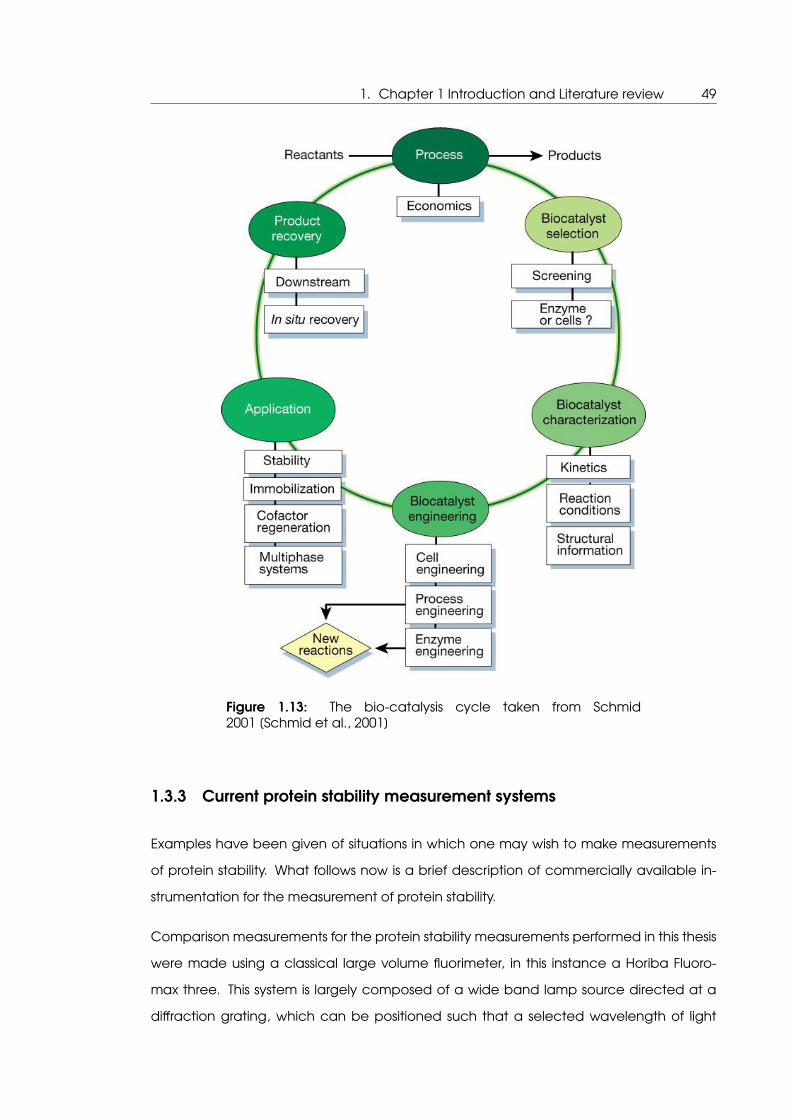
1. Chapter 1 Introduction and Literature review 49
Figure 1.13: The bio-catalysis cycle taken from Schmid2001 [Schmid et al., 2001]
1.3.3 Current protein stability measurement systems
Examples have been given of situations in which one may wish to make measurements
of protein stability. What follows now is a brief description of commercially available in-
strumentation for the measurement of protein stability.
Comparison measurements for the protein stability measurements performed in this thesis
were made using a classical large volume fluorimeter, in this instance a Horiba Fluoro-
max three. This system is largely composed of a wide band lamp source directed at a
diffraction grating, which can be positioned such that a selected wavelength of light
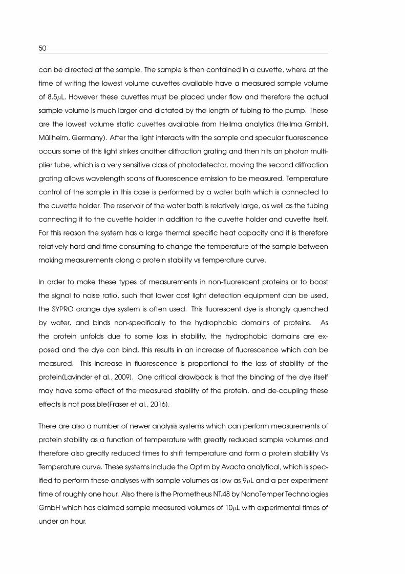
50
can be directed at the sample. The sample is then contained in a cuvette, where at the
time of writing the lowest volume cuvettes available have a measured sample volume
of 8.5µL. However these cuvettes must be placed under flow and therefore the actual
sample volume is much larger and dictated by the length of tubing to the pump. These
are the lowest volume static cuvettes available from Hellma analytics (Hellma GmbH,
Müllheim, Germany). After the light interacts with the sample and specular fluorescence
occurs some of this light strikes another diffraction grating and then hits an photon multi-
plier tube, which is a very sensitive class of photodetector, moving the second diffraction
grating allows wavelength scans of fluorescence emission to be measured. Temperature
control of the sample in this case is performed by a water bath which is connected to
the cuvette holder. The reservoir of the water bath is relatively large, as well as the tubing
connecting it to the cuvette holder in addition to the cuvette holder and cuvette itself.
For this reason the system has a large thermal specific heat capacity and it is therefore
relatively hard and time consuming to change the temperature of the sample between
making measurements along a protein stability vs temperature curve.
In order to make these types of measurements in non-fluorescent proteins or to boost
the signal to noise ratio, such that lower cost light detection equipment can be used,
the SYPRO orange dye system is often used. This fluorescent dye is strongly quenched
by water, and binds non-specifically to the hydrophobic domains of proteins. As
the protein unfolds due to some loss in stability, the hydrophobic domains are ex-
posed and the dye can bind, this results in an increase of fluorescence which can be
measured. This increase in fluorescence is proportional to the loss of stability of the
protein[Lavinder et al., 2009]. One critical drawback is that the binding of the dye itself
may have some effect of the measured stability of the protein, and de-coupling these
effects is not possible[Fraser et al., 2016].
There are also a number of newer analysis systems which can perform measurements of
protein stability as a function of temperature with greatly reduced sample volumes and
therefore also greatly reduced times to shift temperature and form a protein stability Vs
Temperature curve. These systems include the Optim by Avacta analytical, which is spec-
ified to perform these analyses with sample volumes as low as 9µL and a per experiment
time of roughly one hour. Also there is the Prometheus NT.48 by NanoTemper Technologies
GmbH which has claimed sample measured volumes of 10µL with experimental times of
under an hour.
1. Chapter 1 Introduction and Literature review 51
Figure 1.14: Demonstration of the varying size sample holders forbiological analysis systems. a| is the typical volume used in atraditional biological analysis system. b| the sample holder ofthe Avacta Optim cutting edge protein stability analysis systemc| the capillary sample holder used in the experiments detailedin this thesis
For comparison the various size sample holder used in these analysis systems are shown in
1.14 with from left to right the sample size used typically in a traditional cuvette fluorimeter,
the sample holder of a cutting edge instrument such as the Avacta Optim, and finally the
capillary sample holder used in the experiments detailed later on here.
1.3.4 The Green Fluorescent Protein
The Green fluorescent Protein is derived from the jellyfish Aequorea victoria [Tsien, 1998],
it contains a chromophore buried in its centre that exhibits fluorescence. When it is prop-
erly formed GFP exhibits two main absorption peaks at 398 nm and 478 nm, and two
emission peaks at 460 & 510nm [Leiderman et al., 2006]. The GFP gene is frequently in-
serted in experiments in molecular biology to illustrate that transcription of some insert
has occurred[Chalfie et al., 1994]. As with any other protein GFP will become destabi-
lized with increase in temperature, this destabilization will eventually lead to a decrease
in fluorescence as the structure of and around the fluorescent chromophore buried in
the centre becomes disrupted. [Leiderman et al., 2006]. This loss in protein function asso-
ciated with denaturation is considered analogous to the loss in specific function associ-
ated with denaturation in any other protein, and is therefore used later on as a surrogate
for any system exhibiting loss of protein function for temperature increase, albeit with a
readily detectable optical signal.
52
1.4 Mutation patterns of Hepatitis B Virus
One aspect to be developed in this thesis is the use of all-optical thermal control in mi-
crofluidics for performing qPCR. This technique is the clinical ’gold standard’ for the de-
tection of viral copy number in the monitoring of the pathology of viral conditions, such
as in infections by the Hepatitis B Virus . The Hepatitis B Virus is the cause of Hepatitis B
disease which causes death by liver inflammation and cancer. The virus exhibits muta-
tion patterns in reaction to the deployment of anti-viral drugs[Lok and McMahon, 2009],
these patterns were studied to use as a test case for the development of a microfluidic
qPCR disease diagnostic system. To illustrate the practical application of such a system.
The details of this disease diagnostic test case will be elucidated here.
1.4.1 The Hepatitis B virion and its replication cycle
Hepatitis B virus (HBV) is a member of the family Hepadnaviridiae, named for their hep-
atotropism and the fact that the genome is composed of DNA. It is related to other
hepatocyte-infecting viruses within the genus Orthohepadnaviridiae; viruses within this
genus tend to have a similar mode of infection and life cycle but differ in their host
tropism [Thiel et al., 2005]. In 1970, Dane and colleagues established that HBV was the
causative agent of hepatitis type B infection through detailed electron microscopy stud-
ies [Dane et al., 1970]. The intact infectious virions, which are approximately 42nm in size,
are therefore known as Dane particles. Chronic and acute infection by HBV leads to hep-
atitis by way of the adaptive immune responses against the virus, causing inflammation
and tissue damage within the infected hepatocytes[Suhail et al., 2014]. High levels of vi-
raemia occur in vivo in an infected individual and the most common route of transmission
is mediated by fluid exchange [Lee, 1997].
The partially double stranded (ds) DNA genome of HBV is shown in figure 1.15. Open
Reading Frame (ORF) P encodes the viral polymerase enzyme, which contains a re-
verse transcriptase domain [Beck et al., 2002]. ORF C encodes the core protein (HBc),
which forms the protein coat surrounding the viral genome [Beck and Nassal, 2007]. Ad-
ditionally the pre-C section controls the production of a secreted version of the core
protein called the “e antigen” (HBeAg), which is involved in immune evasion by the
virus [Milich et al., 1998]. ORF S encodes the three subunits of the surface antigen (HB-
sAg) [Beck and Nassal, 2007]. The function of ORF X is to encode the HX protein which

1. Chapter 1 Introduction and Literature review 53
is involved in transducing numerous cellular signalling pathways [Rawat et al., 2012]. The
genome of HBV is compact in nature, being only 3.2 kilo bases in length; it has virtually no
intervening non-coding sequences and the various ORFs overlap meaning that a single
section of nucleic acid is used to encode more than one functional protein. For exam-
ple all three sections of ORF S are nested within ORF P5. a diagrammatic representation
of the organization of the HBV genome is shown in figure 1.15.
Figure 1.15: Structure of the HBV genome taken from Lee 1997[Lee, 1997]
The Hepatitis B virion enters the cell via the use of Sodium taurocholate cotrans-
porting polypeptide as a receptor [Yan et al., 2012]. The viral core migrates to
the nucleus where the relaxed circle DNA (rcDNA) encased within the virion is
unpackaged[Schädler and Hildt, 2009]. Host DNA repair mechanisms then covalently
close and fill in the rcDNA to produce a covalently closed circular DNA (cccDNA). This
cccDNA is used as a template for the transcription of the pre-genomic RNA (pgRNA) and
sub genomic transcripts[Schädler and Hildt, 2009]. The pgRNA migrates from the nucleus
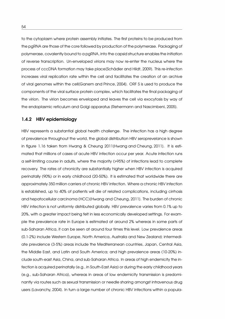
54
to the cytoplasm where protein assembly initiates. The first proteins to be produced from
the pgRNA are those of the core followed by production of the polymerase. Packaging of
polymerase, covalently bound to a pgRNA, into the capsid structure enables the initiation
of reverse transcription. Un-enveloped virions may now re-enter the nucleus where the
process of cccDNA formation may take place[Schädler and Hildt, 2009]. This re-infection
increases viral replication rate within the cell and facilitates the creation of an archive
of viral genomes within the cell[Ganem and Prince, 2004]. ORF S is used to produce the
components of the viral surface protein complex, which facilitates the final packaging of
the virion. The virion becomes enveloped and leaves the cell via exocytosis by way of
the endoplasmic reticulum and Golgi apparatus [Rehermann and Nascimbeni, 2005].
1.4.2 HBV epidemiology
HBV represents a substantial global health challenge. The infection has a high degree
of prevalence throughout the world, the global distribution HBV seroprevelance is shown
in figure 1.16 taken from Hwang & Cheung 2011[Hwang and Cheung, 2011]. It is esti-
mated that millions of cases of acute HBV infection occur per year. Acute infection runs
a self-limiting course in adults, where the majority (>95%) of infections lead to complete
recovery. The rates of chronicity are substantially higher when HBV infection is acquired
perinatally (90%) or in early childhood (20-50%). It is estimated that worldwide there are
approximately 350 million carriers of chronic HBV infection. Where a chronic HBV infection
is established, up to 40% of patients will die of related complications, including cirrhosis
and hepatocellular carcinoma (HCC)[Hwang and Cheung, 2011]. The burden of chronic
HBV infection is not uniformly distributed globally. HBV prevalence varies from 0.1% up to
20%, with a greater impact being felt in less economically developed settings. For exam-
ple the prevalence rate in Europe is estimated at around 2% whereas in some parts of
sub-Saharan Africa, it can be seen at around four times this level. Low prevalence areas
(0.1-2%) include Western Europe, North America, Australia and New Zealand; intermedi-
ate prevalence (3-5%) areas include the Mediterranean countries, Japan, Central Asia,
the Middle East, and Latin and South America; and high prevalence areas (10-20%) in-
clude south-east Asia, China, and sub-Saharan Africa. In areas of high endemicity the in-
fection is acquired perinatally (e.g., in South-East Asia) or during the early childhood years
(e.g., sub-Saharan Africa), whereas in areas of low endemicity transmission is predomi-
nantly via routes such as sexual transmission or needle sharing amongst intravenous drug
users [Lavanchy, 2004]. In turn a large number of chronic HBV infections within a popula-

1. Chapter 1 Introduction and Literature review 55
tion is likely to facilitate a large virus reservoir within that population [Chen et al., 2000].
Figure 1.16: Map showing the global distribution of HBVfrom[Hwang and Cheung, 2011]
HBV has been classified into ten genotypes designated A-J based on a minimum genetic
sequence diversity of 8% [Araujo et al., 2011]. The distribution of different genotypes tends
to be restricted geographically; this is illustrated in Figure 1.17 . In addition to the main
genotypes there are a number of sub-genotypes, for example genotype A is divided into
three sub genotypes A1, A2 & A3. Sub-genotype- A1 is mainly endemic in southern Africa,
A2 mainly within Europe and the United States, with A3 being largely restricted to western
Africa. Furthermore, there are a number of other sub-genotypes that have been found
to exist within the other genotypes [Pujol et al., 2009].

56
Figure 1.17: Geographic distribution of HBV genotypes, where thesize of the genotype letter corresponds to the relative prevelanceof HBV in that region, taken from Pujol 2009 [Pujol et al., 2009]
1.4.3 HIV/HBV co-infection
Human Immunodeficiency Virus (HIV) is a member of the retrovirus family as its
RNA genome is reverse transcribed into DNA by the viral reverse transcriptase en-
zyme [Herschhorn and Hizi, 2010]. The viral DNA is then integrated into the host’s
genome by means of the virally encoded integrase enzyme [Freed and Mouland, 2006].
HIV mainly infects cells of the immune system including CD4+ T cells, macrophages
and dendritic cells. Infection typically results in progressive depletion of CD4+
T cells, chronic immune activation and immunological compromise, which leaves
the host susceptible to opportunistic infections, malignancies, and manifestations
of chronic inflammation, wasting and occasionally dementia (HIV encephalopa-
thy) [Weiss, 1993], [Gallego et al., 2011].
Like HBV, HIV/AIDS is a major global health problem. In 2008, it was estimated that 33.4
million people were infected with HIV-1 [UNAIDS, 2013] and 2.4 million people died of
AIDS [UNAIDS, 2013]. Furthermore, it was estimated that up to 3 million people became
newly infected with HIV. As new infections outstrip those dying of AIDS and as there is no
cure, the number of people infected with HIV continues to increase [UNAIDS, 2013].
The HIV/AIDS epidemic disproportionately affects areas of relatively lower economic de-
velopment, for example the prevalence of HIV in sub-Saharan African adults in 2008
was estimated to be 5.2%, in contrast to Western Europe where it was estimated to be
1. Chapter 1 Introduction and Literature review 57
0.3%. This difference is thought to reflect the much greater accessibility to ART and im-
proved education programmes in the West compared to that of resource-limited set-
tings [UNAIDS, 2013].
HIV co-infection has been shown to accelerate the rate of progression of chronic HBV
infection, leading to marked increases in the number of cases of end-stage liver diseases
including cirrhosis and HCC [Chun et al., 2012]. As HIV-infected patients show improved
survival through ART, they are also more likely to experience the consequences of chronic
HBV infection. Therefore HBV is an emerging co-morbidity of HIV infection and this is of
particular relevance in resource-limited settings where both viruses are highly prevalent
and consequently co-infections are common [Singh and Wong, 2009].
1.4.4 HIV and HBV infection in Malawi
The samples for these studies are drawn from Blantyre in southern Malawi. Malawi is a rel-
atively less economically developed area with high prevalence rates of both HIV and
HBV. Although data are limited, one study reported that HBV co-infection rates were
7% among HIV-infected adults attending the HIV outpatient services in Blantyre, rising
up to 20% among inpatients [Nyirenda et al., 2008]. As seen in the rest of sub-Saharan
Africa, HBV infection typically occurs in early childhood, many years before HIV is ac-
quired. Children may acquire HBV infection directly through close contact with infected
people (e.g., via minor breaks in the skin or mucous membranes) or indirectly via contam-
inated articles such as toothbrushes, razors, or toys [Nyirenda et al., 2008]. HIV-infected
patients in Blantyre are not routinely tested for HBV co-infection and access ART pro-
grammes that are therefore “HBV blind” as they do not take into account the presence
of HBV co-infection. First-line ART regimens typically include lamivudine as the sole agent
with activity against HBV.
1.4.5 Use of Lamivudine in the treatment of HIV & HBV
The first line HIV treatment regimen contains Lamivudine, a nucleoside analogue reverse
transcriptase inhibitor. Lamivudine is an analogue of cytidine; following intracellular phos-
phorylation to its three-phosphate derivative, it competes with the natural substrate for
incorporation into the growing viral DNA chain by HIV reverse transcriptase and HBV
polymerase. However, as it lacks the 3’ hydroxyl group that allows the binding of the
next nucleotide, this causes termination of chain extension and inhibition of viral replica-
58
tion [Lai et al., 1998]. Both HIV and HBV show a low genetic barrier to the emergence of
drug-resistance when Lamivudine is used as mono-therapy. Previous data from HBV in-
fected patients showed that approximately 24% of patients receiving Lamivudine mono-
therapy developed drug-resistance within the first year [Carey and Harrison, 2009]. In HIV
therapy, anti-retroviral drugs are used in combination with other compounds realising a
higher barrier to resistance as a virion that is resistant to one drug is likely to be suppressed
by the other(s) [Sung et al., 2008].
The Polymerase of HBV is known to lack a proof-reading ability and is therefore prone to
introducing errors during viral replication. This means a swarm of genetically heteroge-
neous viruses circulate within an individual. When drugs are introduced, unless suppres-
sion of viral replication is total and the virus is eliminated then over time a drug selective
pressure will be induced[Bartholomeusz and Locarnini, 2006]. HBV infected hepatocytes
contain an archive of cccDNA molecules that will represent the viral quasispecies and
potentially maintain drug resistant mutations in the host.
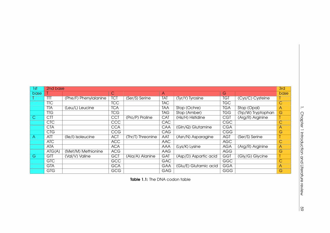
1.C
ha
pte
r1In
trod
uctio
na
nd
Litera
turere
view
59
1st 2nd base 3rdbase T C A G baseT TTT (Phe/F) Phenylalanine TCT (Ser/S) Serine TAT (Tyr/Y) Tyrosine TGT (Cys/C) Cysteine T
TTC TCC TAC TGC CTTA (Leu/L) Leucine TCA TAA Stop (Ochre) TGA Stop (Opal) ATTG TCG TAG Stop (Amber) TGG (Trp/W) Tryptophan G
C CTT CCT (Pro/P) Proline CAT (His/H) Histidine CGT (Arg/R) Arginine TCTC CCC CAC CGC CCTA CCA CAA (Gln/Q) Glutamine CGA ACTG CCG CAG CGG G
A ATT (Ile/I) Isoleucine ACT (Thr/T) Threonine AAT (Asn/N) Asparagine AGT (Ser/S) Serine TATC ACC AAC AGC CATA ACA AAA (Lys/K) Lysine AGA (Arg/R) Arginine AATG[A] (Met/M) Methionine ACG AAG AGG G
G GTT (Val/V) Valine GCT (Ala/A) Alanine GAT (Asp/D) Aspartic acid GGT (Gly/G) Glycine TGTC GCC GAC GGC CGTA GCA GAA (Glu/E) Glutamic acid GGA AGTG GCG GAG GGG G
Table 1.1: The DNA codon table

60
Where specific mutations are discussed, they are referred to in the following manner.
Firstly a code either s or rt, where s implies the mutation is in the open reading frame
that encodes the surface protein, and rt implies the mutation is in the open reading that
encodes the viral polymerase. Next a one letter amino acid code for the wild type amino
acid is given. A numeric position of the mutation in the amino acid chain is then given.
Finally One letter amino acid code of the mutant amino acid is given.
The main lamivudine resistance mutations occur in the catalytic YMDD domain of the re-
verse transcriptase of both HIV and HBV. The methionine at codon 204 (rt204) in HBV is sub-
stituted by valine or isoleucine rtM204V/I [Deny and Zoulim, 2010] Mutation to Isoleucine
tends to be observed in the first instance as the three possible nucleotide changes
that can cause this involve only one nucleotide change whereas three out of the four
changes that would be involved in the switch to Valine involve two nucleotide changes.
This is illustrated using the genetic codon table shown in table 1.1. Where in order to
switch from Methionine to Isoleucine only a change of the final amino acid in the triplet
is required. Whereas in the switch from Methionine to Valine in three of the four possible
permutations the first amino acid as well as last are required.
The rtM204I mutations tend to emerge first, but are subsequently outgrown by the rela-
tively fitter M204V. Virus strains carrying M204V still show a reduction in fitness; however
compensatory mutations that can occur in the polymerase gene, typically involving
codons 80, 173 and 180 can restore the replicative capacity of rtM204V drug resistant
HBV [Lok et al., 2007].
1.4.6 HBsAg mutants
The overlapping ORFs of HBV mean that drug pressure on the polymerase gene (ORF P)
can lead to changes in HBsAg (ORF S), typically at codons s164 (s164) being induced by
changes in position 173 of ORF P. Here a change of Valine to Leucine in ORF P causes
a change from Glutamic Acid to Aspartic Acid in ORF S, this is illustrated in figure1.18.
All possible nucleotide changes that lead to this change in ORF P cause this associated
change in ORF S. Also changes as s195 being concomitant with change at position 204
of ORF P this change can only occur when Methionine is mutated to Valine and not
Isoleucine as the overlap in the codons is only in the first base of position 204 of ORF P,
all possible nucleotide changes that produce a Valine at position 204 of ORF P create a
Methionine in position 195 of ORF S, this is illustrated in 1.19.
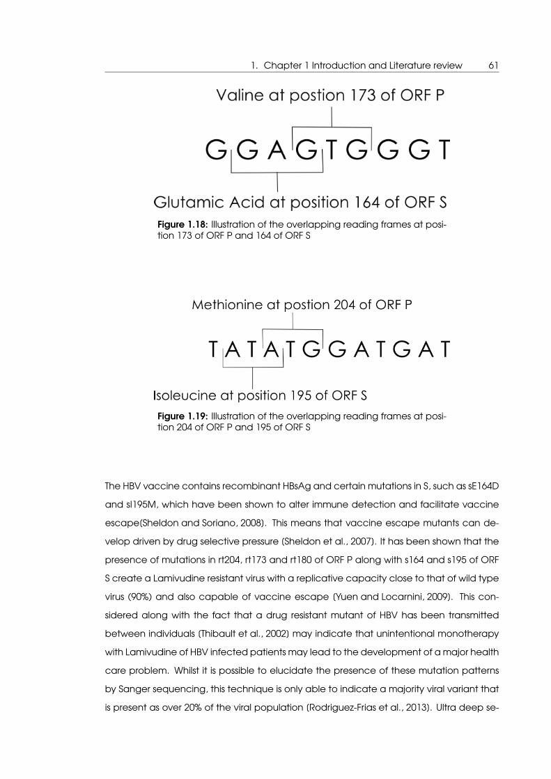
1. Chapter 1 Introduction and Literature review 61
Figure 1.18: Illustration of the overlapping reading frames at posi-tion 173 of ORF P and 164 of ORF S
Figure 1.19: Illustration of the overlapping reading frames at posi-tion 204 of ORF P and 195 of ORF S
The HBV vaccine contains recombinant HBsAg and certain mutations in S, such as sE164D
and sI195M, which have been shown to alter immune detection and facilitate vaccine
escape[Sheldon and Soriano, 2008]. This means that vaccine escape mutants can de-
velop driven by drug selective pressure [Sheldon et al., 2007]. It has been shown that the
presence of mutations in rt204, rt173 and rt180 of ORF P along with s164 and s195 of ORF
S create a Lamivudine resistant virus with a replicative capacity close to that of wild type
virus (90%) and also capable of vaccine escape [Yuen and Locarnini, 2009]. This con-
sidered along with the fact that a drug resistant mutant of HBV has been transmitted
between individuals [Thibault et al., 2002] may indicate that unintentional monotherapy
with Lamivudine of HBV infected patients may lead to the development of a major health
care problem. Whilst it is possible to elucidate the presence of these mutation patterns
by Sanger sequencing, this technique is only able to indicate a majority viral variant that
is present as over 20% of the viral population [Rodriguez-Frias et al., 2013]. Ultra deep se-
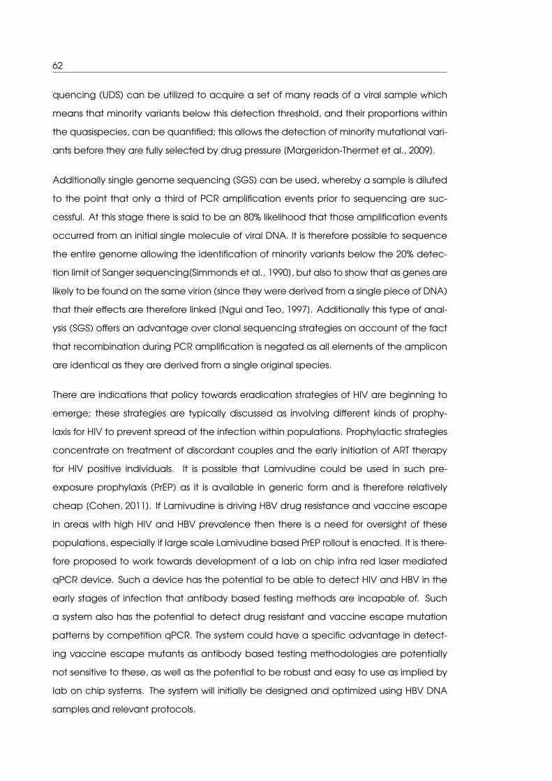
62
quencing (UDS) can be utilized to acquire a set of many reads of a viral sample which
means that minority variants below this detection threshold, and their proportions within
the quasispecies, can be quantified; this allows the detection of minority mutational vari-
ants before they are fully selected by drug pressure [Margeridon-Thermet et al., 2009].
Additionally single genome sequencing (SGS) can be used, whereby a sample is diluted
to the point that only a third of PCR amplification events prior to sequencing are suc-
cessful. At this stage there is said to be an 80% likelihood that those amplification events
occurred from an initial single molecule of viral DNA. It is therefore possible to sequence
the entire genome allowing the identification of minority variants below the 20% detec-
tion limit of Sanger sequencing[Simmonds et al., 1990], but also to show that as genes are
likely to be found on the same virion (since they were derived from a single piece of DNA)
that their effects are therefore linked [Ngui and Teo, 1997]. Additionally this type of anal-
ysis (SGS) offers an advantage over clonal sequencing strategies on account of the fact
that recombination during PCR amplification is negated as all elements of the amplicon
are identical as they are derived from a single original species.
There are indications that policy towards eradication strategies of HIV are beginning to
emerge; these strategies are typically discussed as involving different kinds of prophy-
laxis for HIV to prevent spread of the infection within populations. Prophylactic strategies
concentrate on treatment of discordant couples and the early initiation of ART therapy
for HIV positive individuals. It is possible that Lamivudine could be used in such pre-
exposure prophylaxis (PrEP) as it is available in generic form and is therefore relatively
cheap [Cohen, 2011]. If Lamivudine is driving HBV drug resistance and vaccine escape
in areas with high HIV and HBV prevalence then there is a need for oversight of these
populations, especially if large scale Lamivudine based PrEP rollout is enacted. It is there-
fore proposed to work towards development of a lab on chip infra red laser mediated
qPCR device. Such a device has the potential to be able to detect HIV and HBV in the
early stages of infection that antibody based testing methods are incapable of. Such
a system also has the potential to detect drug resistant and vaccine escape mutation
patterns by competition qPCR. The system could have a specific advantage in detect-
ing vaccine escape mutants as antibody based testing methodologies are potentially
not sensitive to these, as well as the potential to be robust and easy to use as implied by
lab on chip systems. The system will initially be designed and optimized using HBV DNA
samples and relevant protocols.
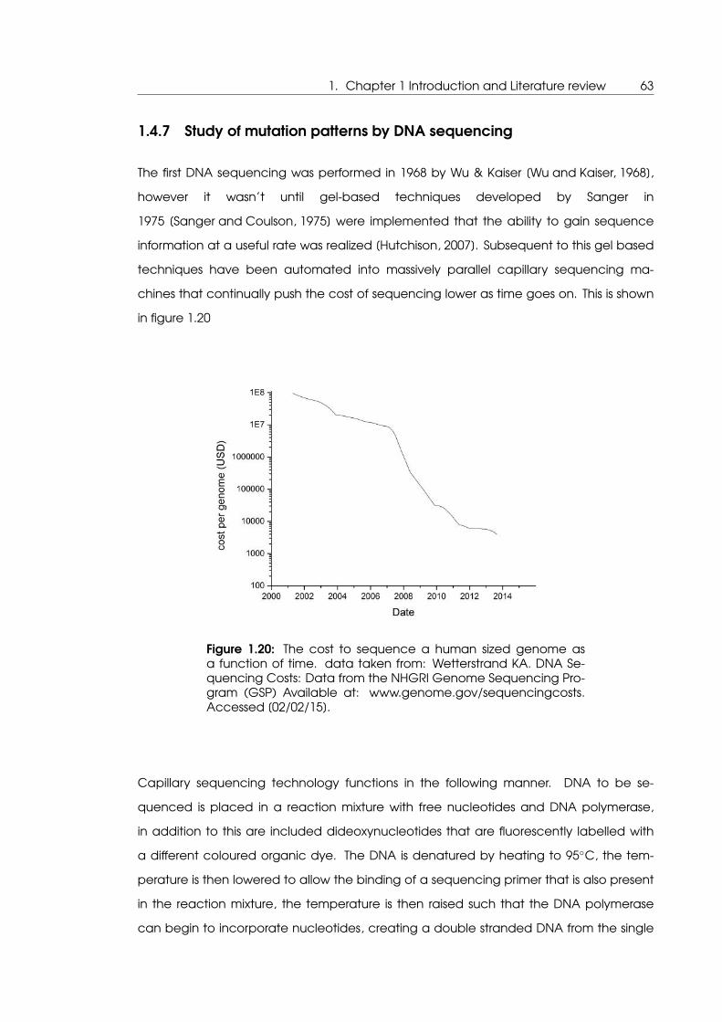
1. Chapter 1 Introduction and Literature review 63
1.4.7 Study of mutation patterns by DNA sequencing
The first DNA sequencing was performed in 1968 by Wu & Kaiser [Wu and Kaiser, 1968],
however it wasn’t until gel-based techniques developed by Sanger in
1975 [Sanger and Coulson, 1975] were implemented that the ability to gain sequence
information at a useful rate was realized [Hutchison, 2007]. Subsequent to this gel based
techniques have been automated into massively parallel capillary sequencing ma-
chines that continually push the cost of sequencing lower as time goes on. This is shown
in figure 1.20
Figure 1.20: The cost to sequence a human sized genome asa function of time. data taken from: Wetterstrand KA. DNA Se-quencing Costs: Data from the NHGRI Genome Sequencing Pro-gram (GSP) Available at: www.genome.gov/sequencingcosts.Accessed [02/02/15].
Capillary sequencing technology functions in the following manner. DNA to be se-
quenced is placed in a reaction mixture with free nucleotides and DNA polymerase,
in addition to this are included dideoxynucleotides that are fluorescently labelled with
a different coloured organic dye. The DNA is denatured by heating to 95◦C, the tem-
perature is then lowered to allow the binding of a sequencing primer that is also present
in the reaction mixture, the temperature is then raised such that the DNA polymerase
can begin to incorporate nucleotides, creating a double stranded DNA from the single

64
stranded DNA template that is to be sequenced. Occasionally a fluorescently labelled
dideoxynucleotide will be included, which, owing to its structure, then induces termina-
tion of chain extension. As the dideoxynucleotides are present in lower concentration
than the regular nucleotides this does not happen often, the result of this overall is that
few double stranded molecules are terminated at perhaps every position along the tem-
plate with a known coloured dye at the termination position. These are then denatured
thermally again such that the terminated fluorescently labelled DNAs at each position
are released from their templates. These are then flowed through a capillary contain-
ing a polymer which is charged electrically. The speed of the DNA molecules migration
through the capillary occurs as a function of their length as with other electrophoretic
techniques. As the DNAs are now ordered by size the coloured dye corresponding to the
position at which termination occurred can be read off optically at some fixed position
on the capillary [Hutchison, 2007].
Such capillary sequencing technology will be used to measure the sequence of the main
population of HBV circulating in individuals in the cohort of study to assess if drug resis-
tance mutations are developing.
Also visible on figure 1.20 is a marked down-turn in the cost around 2007, this is when
second generation or ultra deep sequencing methodologies came online, here the se-
quencing technology is even more massively parallelized. Two competing ultra deep
sequencing technologies are used in this work, those being ’454 sequencing technology’
and ’Illumina sequencing technology’, which will now be detailed.
The first, second generation sequencing technology, to be implemented was ’454 se-
quencing’. In this process polymer beads have single stranded DNAs bound to them that
act as anchors. The DNA to be sequenced has complementary sequences ligated to the
ends. These beads and target DNAs then undergo PCR that has been modified to take
place, in a water and oil emulsion, (emPCR) such that the water micelles form very small
reaction containers, and the target DNA molecules are suitably dilute that each single
bead becomes coated with a homogeneous species of amplified DNA, resultant from a
single strand of target DNA [Tawfik and Griffiths, 1998]. The beads now coated with a ho-
mogenous layer of DNA derived from a single strand of the target DNA are then washed
over plates with bore holes small enough that a single bead-DNA complex will fit in one.
A pyrosequencing reaction then takes place, here an enzyme cascade system is uti-
lized. DNA polymerase is present which on binding of a sequencing primer incorporates
1. Chapter 1 Introduction and Literature review 65
a nucleotide from solution to the corresponding base of the single stranded target DNA
molecule, when this occurs pyrophosphate (PPi) is released, this PPi acts as the substrate
for another enzyme present in solution, that being, ATP-sulfurylase which produces ATP
from this reaction which in turn is the substrate for a reaction using the enzyme luciferase,
which produces a burst of light. In this manner this enzymatic cascade is used to produce
a burst of light for the inclusion of a nucleotide into a double stranded DNA molecule from
a single stranded sequencing target DNA molecule [Ronaghi, 2001]. A 454 sequencing
machine utilizes this process by treating the surface of the plate loaded with DNA coated
beads as an two dimensional array, nucleotides are washed over in succession, when in-
corporation of that nucleotide occurs, because of the pyrosequencing reaction a burst
of light is recorded by a CCD of the system which assigns that nucleotide to that posi-
tion in the array. This is repeated to produce a sequence for each position in the array
with the data being termed a read [Margulies et al., 2005]. The cost advantage comes
in that many array positions are available on the plate and therefore many reads are
produced [Shendure and Ji, 2008]. In the context of measuring the mutational patterns
present in a virally derived sample, all the species present in that sample are read individ-
ually and therefore sub populations of mutant virus can be detected rather than just the
dominating population as is seen with capillary sequencing [Capobianchi et al., 2013].
The other next generation sequencing technology used here is ’Illumina deep sequenc-
ing technology’. A cartoon schematic of how this procedure operates is given in fig-
ure 1.21. This is in some ways similar to 454 sequencing but differs in that the single
stranded DNAs that are the targets of sequencing have adaptor oligonucleotides lig-
ated to both ends, these are then washed over a glass flow cell that has corresponding
oligonucleotides to these adaptor oligonucleotides attached to it. The single stranded
adaptor ligated target sequences bind to the sequences attached to this solid phase
flow cell sparsely. A PCR is then performed on these solid phase bound target DNAs in
which they bridge over to other adaptor sequences bound to the flow cell. This bridge
PCR causes the formation of patches on the flow cell derived from one original bound
target of sequencing DNA species [Voelkerding et al., 2009]. Once these DNA patches
are formed they are denatured leaving only single stranded target DNAs. A sequencing
primer binds, & a mixture of all four nucleotides is added. These nucleotides have been
altered by the addition of a fluorescent dye specific to each type of nucleotide for which
the colour of emission is known, as well as a terminating section that prevents the addi-

66
tion of further nucleotides. After some time the colour of the fluorescent dye bound to
the incorporated nucleotide for that DNA patch is recorded. The dye and terminating
section is then removed and the process repeated to build up the sequence for each
patch. In this context the sequence constructed for each patch constitutes a read.
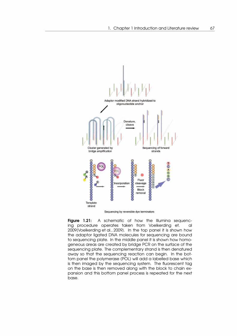
1. Chapter 1 Introduction and Literature review 67
Figure 1.21: A schematic of how the Illumina sequenc-ing procedure operates taken from Voelkerding et. al2009[Voelkerding et al., 2009]. In the top panel it is shown howthe adaptor ligated DNA molecules for sequencing are boundto sequencing plate. In the middle panel it is shown how homo-geneous areas are created by bridge PCR on the surface of thesequencing plate. The complementary strand is then denaturedaway so that the sequencing reaction can begin. In the bot-tom panel the polymerase (POL) will add a labelled base whichis then imaged by the sequencing system. The fluorescent tagon the base is then removed along with the block to chain ex-pansion and this bottom panel process is repeated for the nextbase.

68
There are other second generation sequencing technologies available, 454 was initially
selected as at the time of the experiment it provided the most data per cost. By the
time of the second experiment Illumina technology had surpassed 454 in this respect.
This may reflect a wider picture as Illumina technology has come to dominate the mar-
ketplace [Greenleaf and Sidow, 2014].
1. Chapter 1 Introduction and Literature review 69
1.5 The quantitative Polymerase Chain Reaction in disease
diagnostics
The Polymerase Chain Reaction is a key technique in molecular biology. Here set changes
in temperature in a sample containing DNA in the presence of heat stable DNA polymer-
izing enzymes allow the specific amplification of DNA sequences. This technique has
been made quantifiable by the addition of DNA binding fluorescent dyes, such that the
amplification of these specific sequences can be read out optically, in the quantitative
Polymerase Chain Reaction. This is used as a gold standard test for disease diagnosis
where some pathogenic nucleic acid may be present. In this section it will be discussed
how the techniques of optical thermometry and heating as previously described could
be used to perform qPCR in a microfluidic device.
1.5.1 The Polymerase Chain Reaction and quantitative Polymerase Chain
Reaction
PCR is a core technique of molecular biology. It allows the specific amplification of DNA
targets from complex DNA template molecules such that the amount of target increases
in an exponential manner, facilitating sequencing and detecting of rare species from a
complex background. PCR was initially developed by Kary Mullis at the Cetus corporation
in the late 1970’s, for which he later received the Nobel prize. The work was first detailed
at the Cold Spring Harbor conference of 1986 [Mullis et al., 1992]. The mechanism un-
derlying how PCR operates is detailed in figure 1.22. Initially a complex DNA template is
purified from some cellular extract or other source. A PCR reagent mix is then prepared,
in suitable buffer, which contains some of this template, oligonucleotide primers which
flank some specific DNA target sequence contained within the template, individual nu-
cleotides which will be constructed into the PCR product, a heat stable DNA polymerase
enzyme and its required co-factor magnesium. In the first instance the PCR reagent mix is
heated from room temperature to the point at which the two strands of the DNA template
will separate out from one another, this is somewhere around 95◦C. Once denaturation
of the template has occurred the temperature is dropped to the annealing tempera-
ture of the primer pair, this temperature is dictated by the sequence of the primers but
is nominally in the range of 50◦C - 65◦C. Once the primers have bound to the sequence
specific points on the template molecule the polymerase present in the reagent mix will
70
naturally bind there and begin to extend the complementary strand opposite the tem-
plate molecule, utilizing the nucleotides free in the reagent mix, the temperature is raised
during this process to the optimum operational temperature of the enzyme which is en-
zyme dependent but normally around 72◦C. The first PCR cycle is now complete and the
first round product has been constructed. The temperature is then again raised to the
denaturation temperature of DNA causing the first round product and template to dis-
sociate. Again the temperature is dropped to the annealing temperature of the primer
pairs and then raised to the optimum temperature for construction of the complementary
sequence of the first round product, by the heat stable polymerase. Once the second
round product has been produced by the polymerase the result is two molecules of ev-
ery first round product, the amount of PCR product has likely doubled if 100% efficiency is
assumed, further iterations of the PCR cycling process will lead to further doublings of the
amount of PCR product such that an exponential increase in this product is affected.
The nature of this process means that large amounts of DNA products can be ampli-
fied out of complex DNA background templates which facilitates, among other things,
large scale DNA sequencing work, which in turn has revolutionized molecular biological
research and therefore rational drug development. The economic impact of PCR can
be underlined by the fact that the patent was sold by the Cetus corporation in the mi
1990’s for over 300 million USD [Metzker and Caskey, 2001], a value which can only have
be assumed to have increased vastly since then

1. Chapter 1 Introduction and Literature review 71
Figure 1.22: A schematic representation of the PCR process1| the temperature is raised from ambient to around 95◦C thiscauses the two strands of the DNA template to denature awayfrom each other 2| the temperature is dropped to between50◦C & 65◦C which facilitates binding of the primers, which arepresent in solution, onto the two separate DNA strands 3| Thethermostable DNA polymerase which is present in solution bindsdouble stranded DNA where there is a single strand over hang,such as the primer binding site, additionally the temperature ofthe reaction may be raised here to 72◦C which the optimal tem-perature for the enzymes activity 4| complementary nucleotidesfree in solution are added by the DNA polymerase to form thecomplementary strand of DNA 5| The template DNA moleculeis now present as well as the first round of PCR product 6|thetemperature is again raised to around 95◦C such that the firstround PCR product is denatured into to two separate strands7| the temperature is then again lowered such that the primersand polymerase free in solution can bind to the PCR product 8|the polymerase will then construct the complementary strand asbefore resulting in double the amount of PCR product 9| steps6-8 are repeated resulting in a doubling of the amount of PCRproduct with each cycle until something required for the processsuch as free nucleotides or primers in solution becomes limitingor until the enzymatic activity of the polymerase is degraded.This figure adapted from Textbook of diagnostic microbiology[Mahon et al., 2014]
72
One development of PCR, is quantitative PCR or qPCR, here optical readout mechanisms
are incorporated into the PCR process such that a calculation of the amount of DNA
present can be made. The concept underlying qPCR was first introduced by Higuchi and
collaborators in 1993 [Higuchi et al., 1993]. Here a normal PCR reaction as detailed previ-
ously takes place in the presence of Ethidium Bromide, which has an increased quantum
yield when it is bound intercalating across two complementary bases of DNA as opposed
to when it is free in solution [Goldys, 2009]. This means that as the PCR product accumu-
lates free dye will bind and increase in fluorescence output when excited. This can be
measured using optical means such as using a CCD camera in Higuchi’s work.
For any given PCR reaction where all other variables are controlled apart from the num-
ber of copies of the initial template the rate at which PCR mediated DNA production
occurs will increase as a function of the number of initial copies. qPCR can be used to
measure this rate in real time as the PCR reaction occurs as the fluorecence readout in-
creases as a function of accumulated PCR product amount, on account of this qPCR is
sometimes referred to as real-time PCR. Further developments have been made to the
qPCR process for instance the use of intercalating dyes that are thoughts to have a less
carcinogenic action than ethidium bromide such as SYBR green, but that also show the
same behaviour in terms of an increased fluorescence when bound to DNA as opposed
to when in solution [Cosa et al., 2001]. Additionally there have been alternative meth-
ods made for gaining an optical read out of qPCR, for example the use of FRET probes.
FRET probes in qPCR are small oligonucleotide sequences, located somewhere between
the primers on the target DNA molecule. They differ from primers in that they have flu-
orophores chemically attached at both ends, these fluorophores have an overlapping
emission and excitation spectra, this means that when the first fluorophore is excited it
emits at a wavelength that excites the other fluorophore. This process of passing energy
between fluorophores is known as Förster Resonance Energy Transfer (FRET), the efficiency
of which is highly dependent upon the distance between the fluorophores involved. In a
qPCR FRET probe the first fluorophore is excited and the its fluorescence emission is mea-
sured, most of the energy is passed to the second fluorophore by FRET and therefore a
low fluorescence emission signal is detected. The probe can become integrated into a
PCR product DNA molecule by binding at the specific target sequence and then be-
ing passed over by an approaching PCR polymerase molecule. When the polymerase
molecule passes over, the fluorophores become dissociated from the probe DNA and
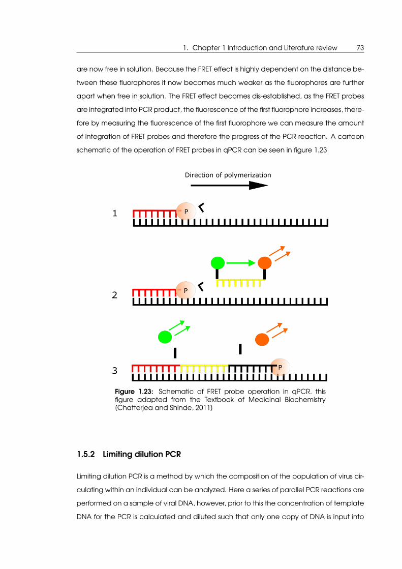
1. Chapter 1 Introduction and Literature review 73
are now free in solution. Because the FRET effect is highly dependent on the distance be-
tween these fluorophores it now becomes much weaker as the fluorophores are further
apart when free in solution. The FRET effect becomes dis-established, as the FRET probes
are integrated into PCR product, the fluorescence of the first fluorophore increases, there-
fore by measuring the fluorescence of the first fluorophore we can measure the amount
of integration of FRET probes and therefore the progress of the PCR reaction. A cartoon
schematic of the operation of FRET probes in qPCR can be seen in figure 1.23
Figure 1.23: Schematic of FRET probe operation in qPCR. thisfigure adapted from the Textbook of Medicinal Biochemistry[Chatterjea and Shinde, 2011]
1.5.2 Limiting dilution PCR
Limiting dilution PCR is a method by which the composition of the population of virus cir-
culating within an individual can be analyzed. Here a series of parallel PCR reactions are
performed on a sample of viral DNA, however, prior to this the concentration of template
DNA for the PCR is calculated and diluted such that only one copy of DNA is input into

74
each PCR reaction. It would follow that when a sample of template DNA is spread out
amongst a number of PCR reactions, the likelihood of a reaction occurring from a single
piece of template DNA increases as the number of reactions that fail to amplify due to
there being no template DNA molecule increases. By using the Poisson series we can say
that
P0 = e−µ (1.9)
which can rearranged to
µ = −lnP0 (1.10)
where P0 are the proportion of reactions containing no DNA i.e. fail to amplify and µ is
the mean number of DNA molecules
and
P1 = µe−µ (1.11)
where P1 are the proportion of reactions containing DNA i.e. they amplify and mu is the
mean number of DNA molecules
which together give
P1 = −P0lnP0 (1.12)
which substituted into
F1 = P1/1− P0 (1.13)
where F1 is the proportion of of successful amplifications that took place from one piece
of DNA, gives
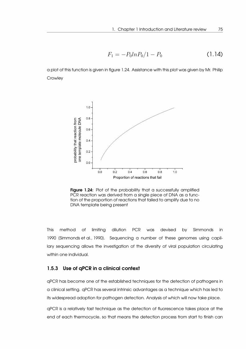
1. Chapter 1 Introduction and Literature review 75
F1 = −P0lnP0/1− P0 (1.14)
a plot of this function is given in figure 1.24. Assistance with this plot was given by Mr. Philip
Crowley
Figure 1.24: Plot of the probability that a successfully amplifiedPCR reaction was derived from a single piece of DNA as a func-tion of the proportion of reactions that failed to amplify due to noDNA template being present
This method of limiting dilution PCR was devised by Simmonds in
1990 [Simmonds et al., 1990]. Sequencing a number of these genomes using capil-
lary sequencing allows the investigation of the diversity of viral population circulating
within one individual.
1.5.3 Use of qPCR in a clinical context
qPCR has become one of the established techniques for the detection of pathogens in
a clinical setting. qPCR has several intrinsic advantages as a technique which has led to
its widespread adoption for pathogen detection. Analysis of which will now take place.
qPCR is a relatively fast technique as the detection of fluorescence takes place at the
end of each thermocycle, so that means the detection process from start to finish can

76
be completed in some cases in under an hour. Other PCR based techniques such a
detection of PCR products using agarose gel electrophoresis require the additional time
to set up run and image the gel. Likewise detection by capillary sequencing would also
require extra time.
PCR can be highly specific, in that the primer sequences are designed to detect a spe-
cific sequence in some pathogen. The probability of the same sequence being found in
some other organism decreases as a function of primer length. qPCR also has this as an
inherent advantage in that the specificity is tunable by design of the length of the primer
sequences.
qPCR has the advantage over other PCR based detection strategies, in that the reaction
and detection take place in the same reaction container. Meaning that the sample
does not have to be removed, for example, to be loaded onto a gel for imaging or onto
a sequencing reaction plate. This reduces the chances of cross-contamination or sample
mix-up.
Because qPCR is quantitative it can give more information than simply the presence or
absence of a pathogen. For example it can be used to give such useful information as
the amount of virus circulating in an individual patient. This ’Viral load’ information is of
clinical importance as a higher amount of circulating virus is often associated with poorer
prognosis and also may indicate that a virus has become resistant to some treatment
methodology. In order to perform this quantification a ’standard’ of known virus concen-
tration is serially diluted and run at the same time as the patient samples. The point in time
at which the increase in fluorescence due to the exponential increase in the amount of
viral DNA due to PCR begins is proportional to the original amount of DNA. Samples with
higher initial DNA concentrations will be seen to be undergoing PCR earlier. So when the
serially diluted sample is run along side the patient sample it provides a measure of the
initial viral DNA concentration of the patient sample. If the patient sample appears to be
undergoing PCR between the point at which two dilutions of the standard starts to un-
dergo PCR, then the concentration of DNA in the patient sample must be between the
concentration of those two dilutions of the standard, which are known. qPCR is therefore
a standard tool for tracking the viral load of patients undergoing anti-viral therapy.
One disadvantage that qPCR has in a clinical context over detection by sequencing
is that inherently no sequence information is derived. This apparently would preclude
qPCR for being used for the detection of viral mutants. However modifications can be
1. Chapter 1 Introduction and Literature review 77
made to qPCR to facilitate the detection of specific mutants. Locked nucleic acids are
modified nucleotides that can be incorporated into qPCR primer and probe sequences.
they have been shown to drastically increase the level of binding specificity of nucleic
acids[Ballantyne et al., 2008]. This increase in binding specificity means that protocols
have been developed to perform single nucleotide mutation detection, an example of
which is the work of Zeng et. al. in which a qPCR protocol was developed to detect the
main Lamivudine resistance mutation using locked nucleic acid probes[Zeng et al., 2014].
It is possible using locked nucleic acid probes to design an experiment to detect any
specific single nucleic acid mutation using a qPCR device. This would be employed to
perform the detection of mutant types elucidated from the sequencing portion of the
experiments presented here in an all optical qPCR device
1.5.4 Commercial qPCR systems
A plethora of qPCR machines are available. What they must all essentially consist of, and
some description of available systems will be undertaken
A thermocycling element of the system must be present in order to perform the PCR. This
would likely be composed of some heating element, which is thermally coupled to a
heat block, this heat block will contain sample tubes. Additionally there would be some
temperature sensing equipment embedded in the heat block such as a thermocouple.
A temperature control feedback loop would be implemented between the tempera-
ture sensor and the heating element such that the temperature of the system could be
made to follow some pre determined PCR program. Variation on this theme have been
attempted such as the ’light cycler’ family of instruments from Roche in which heating of
the sample is enacted by blowing heated air at it. The basic premise remains the same
in that the sample must be heated in a controlled manner, following a PCR program.
The detection element of the PCR system is essentially a fluorimeter, in that visible light
fluorescence is measured to quantify the progress of the reaction. The components of
this element would likely be in most cases: an excitation source, a photo-detector and
some filter so ensure the excitation source does not swamp the fluorescence signal. The
excitation source would likely be either a pressurized gas lamp with a broad output spec-
trum and filters to narrow that spectrum to the absorption spectra of the detection dye
used in the qPCR reagent mix or LEDs matched to those absorption spectra. The detec-
tion system would likely be a photodiode or CCD with filters used to block the excitation
78
source.
The final main element of a commercial qPCR system would be the reaction mixtures
sample containers. These are likely to be disposable plastic tubes, plates of plastic tubes
or glass tubes. The main criteria for these are that they are able to withstand the tem-
peratures involved in PCR and that they are optically transmissible enough to facilitate
detection of the fluorescence signal.
The commercial qPCR system that was used for all experiments detailed in this thesis was
the 7500 fast system by Life technologies. This system takes 96 well plates as the reaction
vessel element of the system. It has a halogen lamp for use as an excitation source and
a CCD camera with filters for use as a detection system. The manufacturers claim a peak
heating rate of 5.5◦C per second. As this heating rate is the limiting factor in which a
qPCR instrument can perform the reaction, the manufacturers claim that this rate means
the system can make measurements of a sample in half an hour.
1.5.5 Fast small scale qPCR systems
As has been illustrated PCR and qPCR are highly valuable techniques used in the field
of disease diagnostics as well as others. Additionally it is true that a high proportion of
time taken during a PCR reaction is in moving between the temperatures required to
denature DNA, anneal primers and extend PCR products. Because of this there has been
a natural progression to utilize smaller sample sizes in PCR and qPCR reactions such that
this ramping time can be shortened and increase analytical throughput of the q/PCR
system.
The ultimate aim in moving to smaller sample sizes in q/PCR systems would be to develop
a microfluidic q/PCR system. And indeed a large body of research work has been devel-
oped towards this aim. A review of this research will now take place.
The first real push to shrink PCR reaction volumes was performed by Northrup and col-
leagues first being announced at the µTAS conference in 1994[Northrup et al., 1995]
and published in 1995[Woolley et al., 1996]. The sample size here at 4-12µl would per-
haps be considered on the high side of what might be considered microfluidics, how-
ever the rationale, in this work, that by driving the sample size of a PCR reaction down
the ramping speed and time to analysis could be reduced, is clear. This is the ratio-
nale that would set the scene for the development of future microfluidic PCR devices.
1. Chapter 1 Introduction and Literature review 79
The Northrup group would move to focus on other microfludics projects some of which
added to the analytic capacity of the microfluidic PCR machine, including a qPCR type
device[Ibrahim et al., 1998].
It should be noted that others such as Peter Wilding were engineering similar, in silicon,
small scale PCR devices around the same time[Wilding et al., 1994] and also moving on
to silicon glass hybrid devices[Shoffner et al., 1996, Cheng et al., 1996] which would pave
the way for all glass devices by others later on. Furthermore ’microchip’ PCR devices
that fit into commercial thermocyclers were developed by Larry Waters and colleagues
that could also be used to perform cell lysis and fluorescent detection of PCR products.
Although in the work of Waters the focus is really on the ’chip’ design rather than shrinking
any of the heat control or detection mechanisms accordingly[Waters et al., 1998].
Other groups were also working on microfluidic PCR devices within a similar time frame.
Work published by Khandurina et. al. in 2000[Khandurina et al., 2000] showed a devi-
ation from the silicon devices shown by the Northrup group earlier, to the use of glass
as a substrate. Here the device is a bespoke ’disposable’ chip with dedicated microflu-
idic channels, which fits into a device with heaters and temperature sensors in contact
with it, and DNA amplification detection optics aligned to it. Here we see the use of
PID control with large K type thermocouples used for temperature detection. Whilst this
work was indeed ground breaking in terms of producing a technology to replace con-
ventional PCR instrumentation, the disposable chips are still vastly more complex and
expensive than conventional reaction tubes. This was followed by other in glass micro
PCR systems[He et al., 2001].
A device with even more complex ’chip’ design is shown at a similar time by Lagally et.
al[Lagally et al., 2000]. which by the integration of microfluidic valves and pumps facili-
tates PCR and electrophoretic analysis on a monolithic device. Whilst this is impressive it
could perhaps be said that the complexity introduced to perform electrophoretic anal-
ysis would be precluded by performing an optical analysis. This work resonates with the
work of a fair few other groups at the time wherein attempts were made to develop mi-
crofluidic devices that were upstream or downstream of PCR such as sample preparation
or analysis[Mueller et al., 2000, Hodko et al., 2001, Belgrader et al., 2000].
At this point the majority of microscale PCR devices were constructed in either silicon or
glass. However in 2002 Yang et. al[Yang et al., 2002]. would report of the first microscale
PCR device in a lost cost plastic ’microchip’. This built on earlier work using larger scale

80
plastic ’PCR pouches’[Findlay et al., 1993]. The reasoning behind using a plastic based
device is that these are of lower cost to manufacture than any device in silicon or glass.
As any commercial PCR system will have to include consumables as a significant portion
of its running cost. Earlier work in the development of microfluidic bio-reactors paved the
way for this[Grodzinski et al., 2001].
Prior to the work by Yang. The group lead by Landers built a similar polymer chip
microscale PCR device. However this was fabricated out of relatively expensive
Polyimide[Giordano et al., 2001]. Another key way in which the device in this work dif-
fers from previous devices is that instead of using some kind of heat block and resistive
heating element thermally coupled to the sample. Instead optical heating is employed.
Wherein an infrared lamp source is focused down on to the sample to provide direct
heating. This facilitates faster ramping temperature rates than in previous systems (of sim-
ilar size), as the system has a lower thermal mass. This was a progression of earlier work by
this group in which an infra red lamp was used for non contact heating to enact PCR in
borosilicate glass wells[Oda et al., 1998] and capillaries[Hühmer and Landers, 2000].
The concept of using infra red non contact heating to perform PCR was later developed
by Dieter Braun and colleagues[Braun et al., 2003], with a modification in that an infra-
red laser source was used rather than a lamp. This simplifies the optical setup of such a
device greatly. In this work they suppose that the convection based PCR occurring in
their device could be a model for the origins of life, as it replicates primordial DNA being
amplified by the heat in the pore of a hydrothermal vent, in the ocean[Braun, 2004],
rather that to push towards some kind of diagnostic device.
The idea of thermally cycling a PCR reaction with an infra-red laser with a view to pro-
ducing a diagnostic device was then taken and developed by several groups. These
typically involved creating micro drops of a PCR reaction mixture in an oil layer, with a
joule heating system used to bring the sample to 60◦C and the infra-red laser heating en-
acted when the denaturation part of the PCR cycle was required[Terazono et al., 2008,
Kim et al., 2009a, Kim et al., 2009b].
Based on these previous works in the literature, it was decided to implement an all optical
qPCR system, that would take on lessons from experience gained in a clinical setting.
These being that sample preparation must be kept simple, such that producing micro
droplets in a mineral oil layer was sub-optimal when compared to pipetting sample into
a microplate or glass capillary. Additionally optical heating would preclude the need for

1. Chapter 1 Introduction and Literature review 81
a joule heating element, simplifying the system and potentially increasing performance
in terms of temperature ramp. Finally the system would be designed to test a real world
clinical problem, that being the tracking of mutational patterns of HBV mutants assessed
elsewhere in this thesis, to add relevancy to the system implementation.

82

2. Chapter 2 Materials & Methods 83
2. Chapter 2 Materials & Methods

84
2.1 Measurement of TAMRA fluorescence Vs Temperature for
optical thermometry
As described a key component of the analyses performed in this project was the use of
optical thermometry to establish the changes in temperature of a solution containing
some biological entities. This method precludes the need for bulky electronic probes in
or around the sample, facilitating a reduction in sample size whilst still allowing accurate
measurement of sample temperature. Here it will be described how this method was
established.
2.1.1 Basic Fluorimetry of TAMRA as a function of temperature
Fluorescence of 5-TAMRA (Thermo Fisher Scientific, Waltham, MA, USA ) was measured
using a Fluoromax 3 spectofluorometer (Horiba Jobin Yvon Kyoto, Japan). TAMRA was
dissolved in ultra pure water at a concentration of 0.025mg/ml. 1ml samples were placed
in a cuvette of path length 10mm and excited with light at a wavelength of 550nm.
Measurement of Stokes shifted fluorescence was made at room temperature (24◦C). The
temperature of the sample was then increased in a stepwise manner by the use of a
water bath connected to the sample holder of the spectrofluorometer. Further recordings
were then made after some time was allowed to facilitate temperature equilibration of
the sample. The fluorescence values relative to the room temperature values as well as
the raw values are plotted in figure 2.1

2. Chapter 2 Materials & Methods 85
Figure 2.1: Plot of fluorescence values of TAMRA as a function oftemperature, given both as raw counts per second on the pho-ton multiplier tube of the fluorimeter and also normalized as apercentage of the room temperature value for all other values
2.1.2 Measurement of TAMRA in a qPCR reaction as a function of temper-
ature
As temperature control in PCR needs to be very tightly controlled it was decided to redo
measurement of TAMRA fluorescence as a function of temperature, as it would be used in
a qPCR reaction mix, as the buffering conditions and the presence of other components
may affect the shape of this function.
This function could then be used as a calibration curve against which an all-optical qPCR
system could calculate the temperature of a small volume sample and adjust the tem-
perature optically in order to perform qPCR.
A solution of TAMRA was produced to a final concentration of 35.25µM in 50µM TRIS buffer
adjusted to pH 8.0 with NaOH, in ultra-pure water. This buffering condition was selected
as it mimicked that of the qPCR reagent mix that would be used in these experiments,
that being the SYBR R© Select Master Mix (Life Technologies Carlsbad, CA, USA). In order

86
to check if the presence of TAMRA would inhibit qPCR reaction or readout, and thereby
what concentration of TAMRA should be used in fluorescence readout of temperature,
qPCR reactions were carried out on the 7500 fast qPCR system (Life Technologies Carls-
bad, CA, USA) in the presence of a concentration gradient of TAMRA. The results of this
experiment are given in figure 2.2, this figure shows three replicates of the same concen-
tration gradient performed at the same time, in the same reaction plate.
- 0 . 5 0 . 0 0 . 5 1 . 0 1 . 5 2 . 0 2 . 5 3 . 0 3 . 5 4 . 01 0 0 0 0
2 0 0 0 0
3 0 0 0 0
4 0 0 0 0
5 0 0 0 0
6 0 0 0 0
differ
ence
in sy
be gr
een f
luores
cenc
e pos
t qPC
R (arb
)
T A M R A c o n c e n t r a t i o n ( µ M )
Figure 2.2: Titration of TAMRA concentration in qPCR reactions togauge if it causes a concentration dependent inhibition of qPCRreadout. Plot is the final fluorescence reading of reaction less theirinitial fluorescence reading for TAMRA concentration present inthe reaction
As the experiment described by figure 2.2 did not appear to show any appreciable in-
hibition of qPCR readout for the highest concentration of TAMRA present in the reaction
(3.525µM), it was decided to use this concentration of TAMRA fluorescence readout of
temperature.
In the first instance TAMRA solution at 3.525µM was measured in a 7500 fast qPCR system,
where temperature was stepped up 1◦C and measurement of the fluorescence made
iteratively from 20◦C to 95◦C, the fluorescence data are then reported as a proportion of
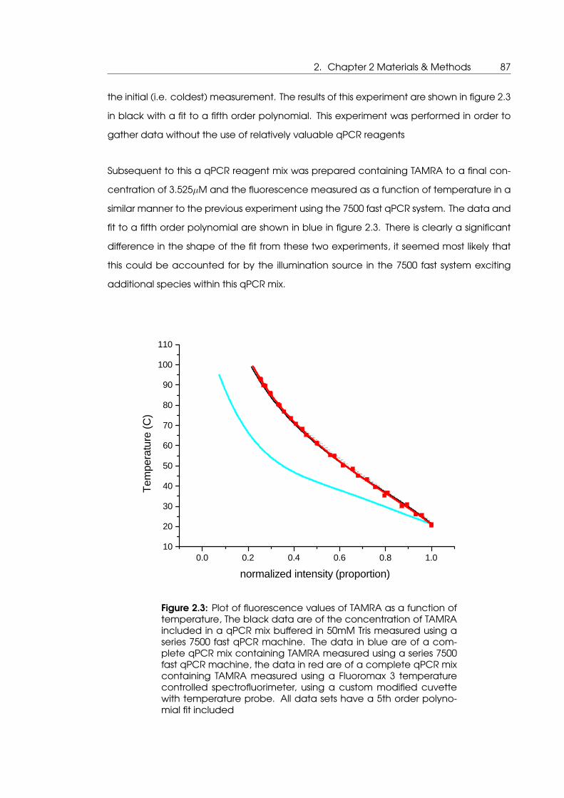
2. Chapter 2 Materials & Methods 87
the initial (i.e. coldest) measurement. The results of this experiment are shown in figure 2.3
in black with a fit to a fifth order polynomial. This experiment was performed in order to
gather data without the use of relatively valuable qPCR reagents
Subsequent to this a qPCR reagent mix was prepared containing TAMRA to a final con-
centration of 3.525µM and the fluorescence measured as a function of temperature in a
similar manner to the previous experiment using the 7500 fast qPCR system. The data and
fit to a fifth order polynomial are shown in blue in figure 2.3. There is clearly a significant
difference in the shape of the fit from these two experiments, it seemed most likely that
this could be accounted for by the illumination source in the 7500 fast system exciting
additional species within this qPCR mix.
0 . 0 0 . 2 0 . 4 0 . 6 0 . 8 1 . 01 02 03 04 05 06 07 08 09 0
1 0 01 1 0
Temp
eratur
e (C)
n o r m a l i z e d i n t e n s i t y ( p r o p o r t i o n )
Figure 2.3: Plot of fluorescence values of TAMRA as a function oftemperature, The black data are of the concentration of TAMRAincluded in a qPCR mix buffered in 50mM Tris measured using aseries 7500 fast qPCR machine. The data in blue are of a com-plete qPCR mix containing TAMRA measured using a series 7500fast qPCR machine, the data in red are of a complete qPCR mixcontaining TAMRA measured using a Fluoromax 3 temperaturecontrolled spectrofluorimeter, using a custom modified cuvettewith temperature probe. All data sets have a 5th order polyno-mial fit included
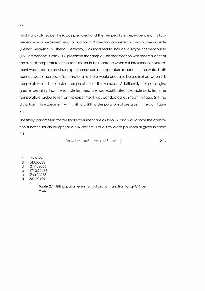
88
Finally a qPCR reagent mix was prepared and the temperature dependence of its fluo-
rescence was measured using a Fluoromax 3 spectofluorometer. A low volume cuvette
(Hellma Analytics, Müllheim, Germany) was modified to include a K-type thermocouple
(RS Components, Corby, UK) present in the sample. This modification was made such that
the actual temperature of the sample could be recorded when a fluorescence measure-
ment was made, as previous experiments used a temperature readout on the water bath
connected to the spectofluorometer and there would of course be a offset between this
temperature and the actual temperature of the sample. Additionally this could give
greater certainty that the sample temperature had equilibrated. Example data from the
temperature probe taken as this experiment was conducted as shown in figure 2.4 The
data from this experiment with a fit to a fifth order polynomial are given in red on figure
2.3.
The fitting parameters for the final experiment are as follows, and would form the calibra-
tion function for an all optical qPCR device. For a fifth order polynomial given in table
2.1
g(x) = ax5 + bx4 + cx3 + dx2 + ex+ f (2.1)
f 175.63296d -543.65892d 1217.82663c -1713.36638b 1266.50688a -381.91404
Table 2.1: fitting parameters for calibration function for qPCR de-vice
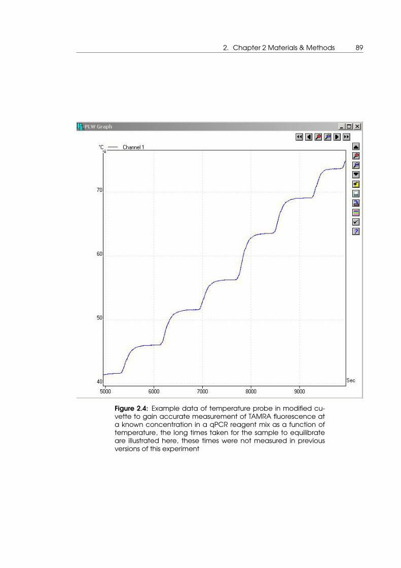
2. Chapter 2 Materials & Methods 89
Figure 2.4: Example data of temperature probe in modified cu-vette to gain accurate measurement of TAMRA fluorescence ata known concentration in a qPCR reagent mix as a function oftemperature, the long times taken for the sample to equilibrateare illustrated here, these times were not measured in previousversions of this experiment
90
2.2 Measurement of GFP stability as a function of tempera-
ture
The butterfly mount was sourced by Dr. Matthieu Gaudet. And the power supply was
sourced By Dr. Sagar Dodderi.
The fluorescence of GFP is related to the integrity of its 3D structure, here a microfluidic
system was created to measure this change in fluorescence as a function of tempera-
ture, mediated by optical heating and measured with optical thermometry, such that
this measurement could be made at a fraction of the sample size and in a fraction of
the analysis time of currently available instrumentation. The construction of this analysis
system will be described here
2.2.1 GFP thermal stability system physical construction

2. Chapter 2 Materials & Methods 91
Figure 2.5: Photograph of the physical construction of the GFPthermal stability measurement system, a custom made butterflymount (B) holds a capillary tube (C) containing protein samplethe arrow indicates the potential direction of flow, the red arrowindicates where an embedded fibre can be used to direct theIR laser energy at the sample. The capillary is clamped into theIR beam path with the setting tool (S). data collection is enactedby imaging using a confocal microscope onto the stage of whichthe entire custom sample mount is bolted
The system for performing analysis of GFP stability was constructed in the following man-
ner. A custom made butterfly stage was designed and built (RoMack Inc., Williamsburg,
VA, USA. Now a part of LEONI Fiber Optics, Inc., Williamsburg, VA, USA). This mount was
designed such that single mode fibre optic lines embedded in blocks would be able
to direct energy from an infrared telecommunications laser, in this case a fibre coupled
(fc/pc connector) 1460nm single mode laser (model number FOL1460, Furokawa elec-
tric, Tokyo, Japan) at a microcapillary (internal diameter 150µm outer diameter 360µm
Upchurch scientific Oak Harbour, WA, USA). The coating on the exterior of the capillary
was removed by the use of a blowtorch, in order to make it optically addressable. Figure
2.5 illustrates the construction of this custom sample mount. This capillary would serve as
the sample holder, containing in this case GFP (rTurboGFP, Evrogen, Moscow, Russia). To
92
perform data capture the sample mount containing the sample loaded into the capil-
lary was bolted onto the stage of a laser scanning confocal microscope (IX81, Olympus,
Center Valley, PA, USA). Excitation of the TAMRA and GFP was performed by the use of
lasers emitting at 532nm and 488nm respectively. The lasers were raster scanned over a
section of the capillary centered around the output of the fibre optic line onto which the
infra-red laser was connected, images of these raster scans were then constructed by
the microscope software.
2.2.2 GFP thermal stability system data analysis methodology
A calibration experiment was performed to assess at what level of power supply to the
IR laser would sufficient temperature change be induced within the sample to cause
denaturation of GFP. The results of this experiment are shown in figure 2.6. Here images
were taken of GFP and TAMRA fluorescence, for a variety of input power levels to the infra
red laser. Temperature of the sample was calculated from TAMRA fluorescence relative
to room temperature images and the calibration experiments for optical thermometry
described earlier.
It should be noted that as the relationship between TAMRA fluorescence and tempera-
ture is non-linear, on account of this whilst the "fluorescence intensity" axis of figure 2.6 is
linear, the corresponding temperature axis is not.
From this experiment it was determined that an input power to the IR laser of 120mW
would be sufficient to put the sample in a temperature range at which GFP denaturation
measured by a decrease in its fluorescence would be induced. A sample containing
TAMRA and GFP was then exposed to this IR laser power, and images were acquired for
the fluorescence of GFP and TAMRA concurrently every 30 seconds, with each image
scan taking 2.6 seconds, this was performed for ten minutes. This means that for any point
in the capillary the temperature was known and the rate of GFP fluorescence loss was
recorded for circa 10◦C sections and the rate of this was calculated by fitting the data of
GFP fluorescence during this experiment to the equation:
y = aexp(−kt) + c (2.2)
where a is the signal amplitude, c is the fluorescence signal decay endpoint, and k is the
rate constant for the fluorescence signal decay associated with GFP denaturation.
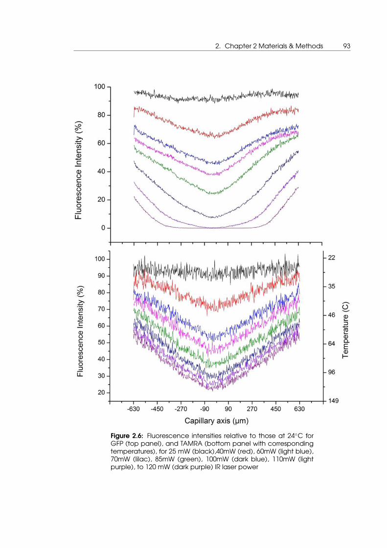
2. Chapter 2 Materials & Methods 93
Figure 2.6: Fluorescence intensities relative to those at 24◦C forGFP (top panel), and TAMRA (bottom panel with correspondingtemperatures), for 25 mW (black),40mW (red), 60mW (light blue),70mW (lilac), 85mW (green), 100mW (dark blue), 110mW (lightpurple), to 120 mW (dark purple) IR laser power
94
2.3 Analysis of HBV mutational patterns in a cohort of HIV co-
infected Malawians
As described the development of mutational patterns of HBV in a cohort of HIV co-
infected Malawians was used as a test case for the development of a microfluidic qPCR
disease detection system. In order to perform this, general sequencing of the mutational
patterns of HBV within the cohort was performed as well as more detailed establishment
of the quasispecies of HBV circulating within individuals with various methods that will be
detailed in this section, The methods and results from this experimental set were reported
in Clinical Infectious Diseases[Aoudjane et al., 2014].
2.3.1 Study population
Patients were recruited into the study from those presenting with suspected HIV to the
Queen Elizabeth Central Hospital in Blantyre, Malawi. and were selected to start a fixed
dose treatment of stavudine/lamivudine/nevirapine in 2007-2009. Patients were selected
for this treatment course if they had a measured CD4 cell count of below 250cells/ml
or stage 3 or 4 disease as categorized by the World Health Organizations pre existing
criteria. Patient serum and plasma samples were taken from the patients on initiation of
therapy and at six and twelve months post initiation of therapy. Patient samples were
stored at -80◦C for transport to the UK for analysis. The College of Medicine Research &
Ethics Committee, of the University of Malawi, approved the study, and it was conducted
in accordance with the principles of the declaration of Helsinki.
2.3.2 Population sequencing of HBV mutational patterns
Extraction of DNA for patient samples for population sequencing was performed using
the QIAsymphony automated liquid handling system using the standard DNA extraction
reagent kit and protocol (Qiagen, Hilden, Germany). The basic operation of this system is
as follows. Cell lysate is introduced into a reaction tube, into this are introduced charged
magnetic beads. The DNA, being charged, attaches to these (opposite) charged mag-
netic beads. A magnetic rod is then introduced into the reaction tube, the magnetic
beads with bound DNA are attracted and attach to this magnetic rod. This assembly is
then moved to an elution buffer and the DNA is detached from the magnetic beads by
a series of washing steps.
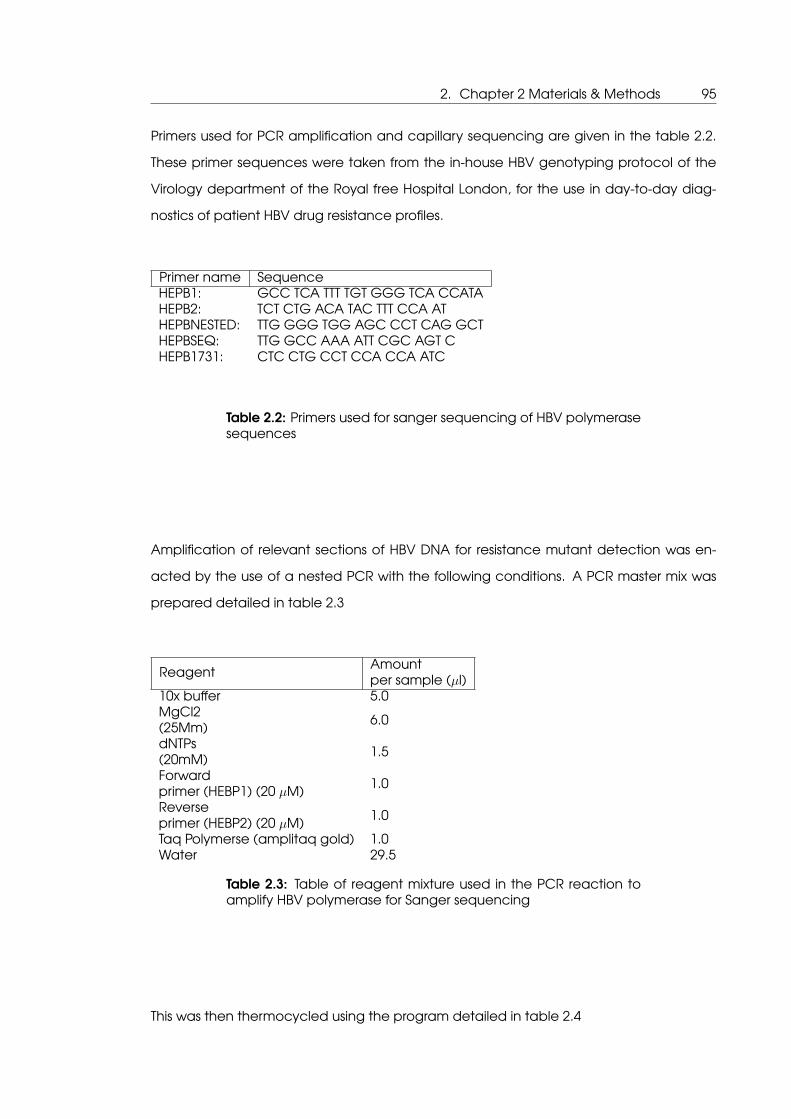
2. Chapter 2 Materials & Methods 95
Primers used for PCR amplification and capillary sequencing are given in the table 2.2.
These primer sequences were taken from the in-house HBV genotyping protocol of the
Virology department of the Royal free Hospital London, for the use in day-to-day diag-
nostics of patient HBV drug resistance profiles.
Primer name SequenceHEPB1: GCC TCA TTT TGT GGG TCA CCATAHEPB2: TCT CTG ACA TAC TTT CCA ATHEPBNESTED: TTG GGG TGG AGC CCT CAG GCTHEPBSEQ: TTG GCC AAA ATT CGC AGT CHEPB1731: CTC CTG CCT CCA CCA ATC
Table 2.2: Primers used for sanger sequencing of HBV polymerasesequences
Amplification of relevant sections of HBV DNA for resistance mutant detection was en-
acted by the use of a nested PCR with the following conditions. A PCR master mix was
prepared detailed in table 2.3
ReagentAmountper sample (µl)
10x buffer 5.0MgCl2(25Mm) 6.0
dNTPs(20mM) 1.5
Forwardprimer (HEBP1) (20 µM) 1.0
Reverseprimer (HEBP2) (20 µM) 1.0
Taq Polymerse (amplitaq gold) 1.0Water 29.5
Table 2.3: Table of reagent mixture used in the PCR reaction toamplify HBV polymerase for Sanger sequencing
This was then thermocycled using the program detailed in table 2.4
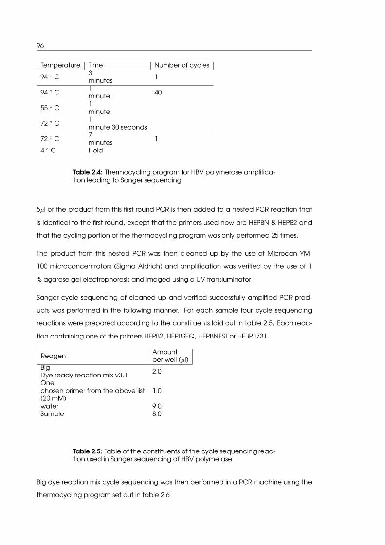
96
Temperature Time Number of cycles
94 ◦ C3minutes 1
94 ◦ C1minute 40
55 ◦ C1minute
72 ◦ C1minute 30 seconds
72 ◦ C7minutes 1
4 ◦ C Hold
Table 2.4: Thermocycling program for HBV polymerase amplifica-tion leading to Sanger sequencing
5µl of the product from this first round PCR is then added to a nested PCR reaction that
is identical to the first round, except that the primers used now are HEPBN & HEPB2 and
that the cycling portion of the thermocycling program was only performed 25 times.
The product from this nested PCR was then cleaned up by the use of Microcon YM-
100 microconcentrators (Sigma Aldrich) and amplification was verified by the use of 1
% agarose gel electrophoresis and imaged using a UV transluminator
Sanger cycle sequencing of cleaned up and verified successfully amplified PCR prod-
ucts was performed in the following manner. For each sample four cycle sequencing
reactions were prepared according to the constituents laid out in table 2.5. Each reac-
tion containing one of the primers HEPB2, HEPBSEQ, HEPBNEST or HEBP1731
ReagentAmountper well (µl)
BigDye ready reaction mix v3.1 2.0
Onechosen primer from the above list(20 mM)
1.0
water 9.0Sample 8.0
Table 2.5: Table of the constituents of the cycle sequencing reac-tion used in Sanger sequencing of HBV polymerase
Big dye reaction mix cycle sequencing was then performed in a PCR machine using the
thermocycling program set out in table 2.6
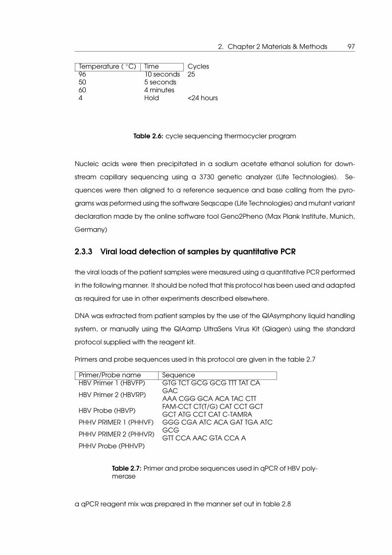
2. Chapter 2 Materials & Methods 97
Temperature ( ◦C) Time Cycles96 10 seconds 2550 5 seconds60 4 minutes4 Hold <24 hours
Table 2.6: cycle sequencing thermocycler program
Nucleic acids were then precipitated in a sodium acetate ethanol solution for down-
stream capillary sequencing using a 3730 genetic analyzer (Life Technologies). Se-
quences were then aligned to a reference sequence and base calling from the pyro-
grams was peformed using the software Seqscape (Life Technologies) and mutant variant
declaration made by the online software tool Geno2Pheno (Max Plank Institute, Munich,
Germany)
2.3.3 Viral load detection of samples by quantitative PCR
the viral loads of the patient samples were measured using a quantitative PCR performed
in the following manner. It should be noted that this protocol has been used and adapted
as required for use in other experiments described elsewhere.
DNA was extracted from patient samples by the use of the QIAsymphony liquid handling
system, or manually using the QIAamp UltraSens Virus Kit (Qiagen) using the standard
protocol supplied with the reagent kit.
Primers and probe sequences used in this protocol are given in the table 2.7
Primer/Probe name SequenceHBV Primer 1 (HBVFP) GTG TCT GCG GCG TTT TAT CA
HBV Primer 2 (HBVRP)GACAAA CGG GCA ACA TAC CTT
HBV Probe (HBVP)FAM-CCT CT(T/G) CAT CCT GCTGCT ATG CCT CAT C-TAMRA
PHHV PRIMER 1 (PHHVF) GGG CGA ATC ACA GAT TGA ATC
PHHV PRIMER 2 (PHHVR)GCGGTT CCA AAC GTA CCA A
PHHV Probe (PHHVP)
Table 2.7: Primer and probe sequences used in qPCR of HBV poly-merase
a qPCR reagent mix was prepared in the manner set out in table 2.8

98
Reagent Amount per sample µlUniversal Mastertmix 26HBV Forward Primer (0.5µM) 2HBV Reverse Primer (0.5µM) 2PHHV Forward Primer (0.5µM) 2PHHV Reverse Primer (0.5µM) 2HBV Probe (0.25µM) 1PHHV Probe (0.5µM) 1Water 1
Table 2.8: HBV pol qPCR reagent mixture
The universal mastermix was TaqMan Universal Master Mix II (Life Technologies) with 14µL
of sample added to each reaction mix. Samples were run against a seven part 1 in ten
dilution series of the WHO HBV standard to calibrate concentration. Additionally an con-
trol internal control reaction was performed in each reaction with template primers and
probes derived from the Phocine herpesvirus 1 (PhHV-1). Samples were analyzed using
the Fast 7500 qPCR system (Life Technologies) using a standard two-step PCR program
and the manufacturers standard sample plates. Analysis of results was performed by the
software included with the Fast 7500 qPCR system.
2.3.4 HBV quasispecies analysis by limiting dilution whole genome PCR
DNA was extracted from patient samples by the use of the QIAsymphony liquid handling
system, or manually using the QIAamp UltraSens Virus Kit (Qiagen) using the standard
protocol supplied with the reagent kit.
The number of viral DNA copies in each extract was measured for each sample using
the HBV qPCR protocol described previously. The objective of this protocol is to dilute
the sample such that only a single copy of template DNA is present in each sample.
The amount of extracted DNA that would contain 93 copies of viral DNA was calculated
and diluted into into 465 µL of water. A 96 well PCR reaction plate was then set up as in
figure 2.7. The positive control reaction was a high titre, non diluted sample. The reagents
required to set up the reaction plate are described in table 2.9

2. Chapter 2 Materials & Methods 99
Reagent Amount to prepare plate µlPCR buffer 475MgCl2 285dNTP 95Primer f 237.5Pprimer r 237.5Enzyme 49.4DNA 475water 2800.6
Table 2.9: HBV limiting dilution whole genome PCR reagent mix-ture constituents
The polymerase enzyme PCR buffer, dNTPs & MgCl2 are derived from the Expand High
Fidelity PLUS PCR System (Roche, Basel, Switzerland)
Primer sequences for the first round plate are given in table 2.10
Primer Name Primer sequencePrimer P1_AE CAC CTC TGC CTA ATC ATC TCT TGT TCA TGPrimer P2_AE AAA AAG TTG CAT GGT GCT GGT GCG CAG AC
Table 2.10: First round primer sequences for limiting dilution wholegenome PCR
and thermocycling conditions are given in the following table 2.11
Temperature Time Number of cycles
94 ◦ C3minutes 1
94 ◦ C1minute 35
54 ◦ C1minute
72 ◦ C1minute 30 seconds
72 ◦ C7minutes 1
4 ◦ C Hold
Table 2.11: First round thermocycling program for limiting dilutionwhole genome PCR
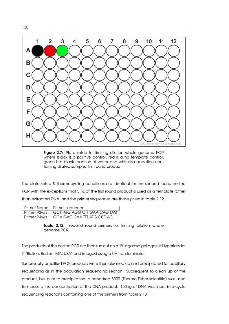
100
Figure 2.7: Plate setup for limiting dilution whole genome PCRwhere black is a positive control, red is a no template control,green is a blank reaction of water and white is a reaction con-taining diluted sample/ first round product
The plate setup & thermocycling conditions are identical for the second round nested
PCR with the exceptions that 5 µL of the first round product is used as a template rather
than extracted DNA, and the primer sequences are those given in table 2.12.
Primer Name Primer sequencePrimer P3wrs GCT TGG AGG CTT GAA CAG TAGPrimer P4wrs GCA GAC CAA TTT ATG CCT AC
Table 2.12: Second round primers for limiting dilution wholegenome PCR
The products of the nested PCR are then run out on a 1% agarose gel against Hyperladder
III (Bioline, Boston, MA, USA) and imaged using a UV transluminator.
Successfully amplified PCR products were then cleaned up and precipitated for capillary
sequencing as in the population sequencing section. Subsequent to clean up of the
product, but prior to precipitation, a nanodrop 8000 (Thermo Fisher scientific) was used
to measure the concentration of the DNA product. 150ng of DNA was input into cycle
sequencing reactions containing one of the primers from table 2.13
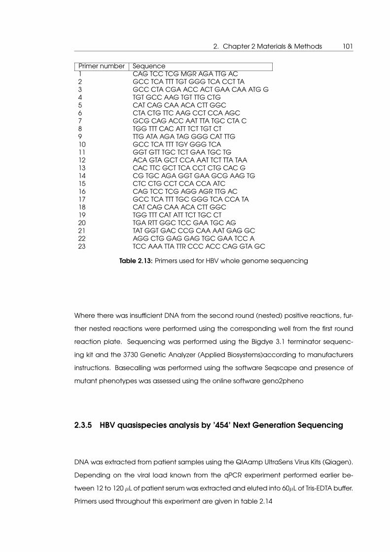
2. Chapter 2 Materials & Methods 101
Primer number Sequence1 CAG TCC TCG MGR AGA TTG AC2 GCC TCA TTT TGT GGG TCA CCT TA3 GCC CTA CGA ACC ACT GAA CAA ATG G4 TGT GCC AAG TGT TTG CTG5 CAT CAG CAA ACA CTT GGC6 CTA CTG TTC AAG CCT CCA AGC7 GCG CAG ACC AAT TTA TGC CTA C8 TGG TTT CAC ATT TCT TGT CT9 TTG ATA AGA TAG GGG CAT TTG10 GCC TCA TTT TGY GGG TCA11 GGT GTT TGC TCT GAA TGC TG12 ACA GTA GCT CCA AAT TCT TTA TAA13 CAC TTC GCT TCA CCT CTG CAC G14 CG TGC AGA GGT GAA GCG AAG TG15 CTC CTG CCT CCA CCA ATC16 CAG TCC TCG AGG AGR TTG AC17 GCC TCA TTT TGC GGG TCA CCA TA18 CAT CAG CAA ACA CTT GGC19 TGG TTT CAT ATT TCT TGC CT20 TGA RTT GGC TCC GAA TGC AG21 TAT GGT GAC CCG CAA AAT GAG GC22 AGG CTG GAG GAG TGC GAA TCC A23 TCC AAA TTA TTR CCC ACC CAG GTA GC
Table 2.13: Primers used for HBV whole genome sequencing
Where there was insufficient DNA from the second round (nested) positive reactions, fur-
ther nested reactions were performed using the corresponding well from the first round
reaction plate. Sequencing was performed using the Bigdye 3.1 terminator sequenc-
ing kit and the 3730 Genetic Analyzer (Applied Biosystems)according to manufacturers
instructions. Basecalling was performed using the software Seqscape and presence of
mutant phenotypes was assessed using the online software geno2pheno
2.3.5 HBV quasispecies analysis by ’454’ Next Generation Sequencing
DNA was extracted from patient samples using the QIAamp UltraSens Virus Kits (Qiagen).
Depending on the viral load known from the qPCR experiment performed earlier be-
tween 12 to 120 µL of patient serum was extracted and eluted into 60µL of Tris-EDTA buffer.
Primers used throughout this experiment are given in table 2.14
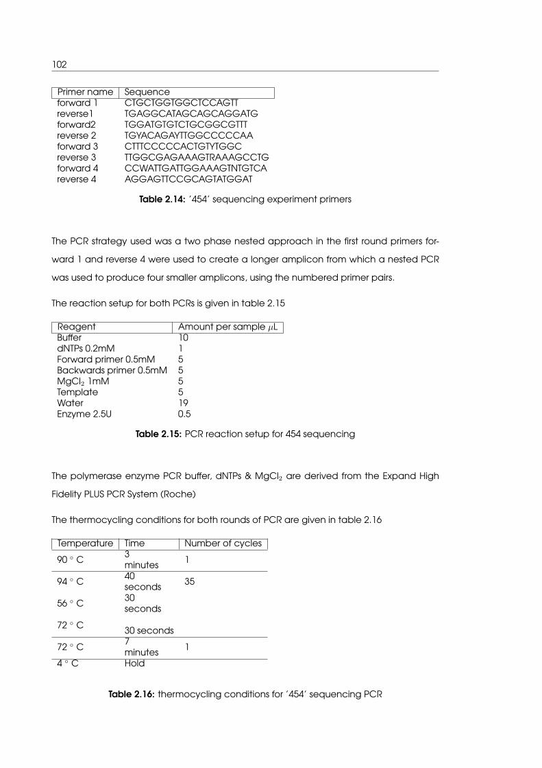
102
Primer name Sequenceforward 1 CTGCTGGTGGCTCCAGTTreverse1 TGAGGCATAGCAGCAGGATGforward2 TGGATGTGTCTGCGGCGTTTreverse 2 TGYACAGAYTTGGCCCCCAAforward 3 CTTTCCCCCACTGTYTGGCreverse 3 TTGGCGAGAAAGTRAAAGCCTGforward 4 CCWATTGATTGGAAAGTNTGTCAreverse 4 AGGAGTTCCGCAGTATGGAT
Table 2.14: ’454’ sequencing experiment primers
The PCR strategy used was a two phase nested approach in the first round primers for-
ward 1 and reverse 4 were used to create a longer amplicon from which a nested PCR
was used to produce four smaller amplicons, using the numbered primer pairs.
The reaction setup for both PCRs is given in table 2.15
Reagent Amount per sample µLBuffer 10dNTPs 0.2mM 1Forward primer 0.5mM 5Backwards primer 0.5mM 5MgCl2 1mM 5Template 5Water 19Enzyme 2.5U 0.5
Table 2.15: PCR reaction setup for 454 sequencing
The polymerase enzyme PCR buffer, dNTPs & MgCl2 are derived from the Expand High
Fidelity PLUS PCR System (Roche)
The thermocycling conditions for both rounds of PCR are given in table 2.16
Temperature Time Number of cycles
90 ◦ C3minutes 1
94 ◦ C40seconds 35
56 ◦ C30seconds
72 ◦ C 30 seconds
72 ◦ C7minutes 1
4 ◦ C Hold
Table 2.16: thermocycling conditions for ’454’ sequencing PCR
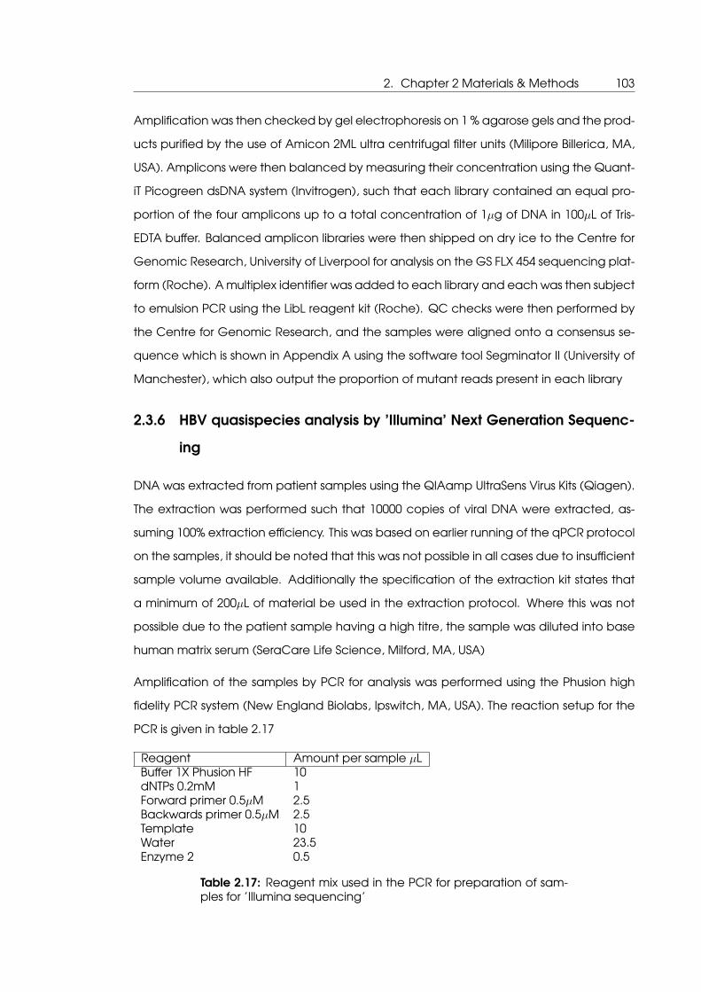
2. Chapter 2 Materials & Methods 103
Amplification was then checked by gel electrophoresis on 1 % agarose gels and the prod-
ucts purified by the use of Amicon 2ML ultra centrifugal filter units (Milipore Billerica, MA,
USA). Amplicons were then balanced by measuring their concentration using the Quant-
iT Picogreen dsDNA system (Invitrogen), such that each library contained an equal pro-
portion of the four amplicons up to a total concentration of 1µg of DNA in 100µL of Tris-
EDTA buffer. Balanced amplicon libraries were then shipped on dry ice to the Centre for
Genomic Research, University of Liverpool for analysis on the GS FLX 454 sequencing plat-
form (Roche). A multiplex identifier was added to each library and each was then subject
to emulsion PCR using the LibL reagent kit (Roche). QC checks were then performed by
the Centre for Genomic Research, and the samples were aligned onto a consensus se-
quence which is shown in Appendix A using the software tool Segminator II (University of
Manchester), which also output the proportion of mutant reads present in each library
2.3.6 HBV quasispecies analysis by ’Illumina’ Next Generation Sequenc-
ing
DNA was extracted from patient samples using the QIAamp UltraSens Virus Kits (Qiagen).
The extraction was performed such that 10000 copies of viral DNA were extracted, as-
suming 100% extraction efficiency. This was based on earlier running of the qPCR protocol
on the samples, it should be noted that this was not possible in all cases due to insufficient
sample volume available. Additionally the specification of the extraction kit states that
a minimum of 200µL of material be used in the extraction protocol. Where this was not
possible due to the patient sample having a high titre, the sample was diluted into base
human matrix serum (SeraCare Life Science, Milford, MA, USA)
Amplification of the samples by PCR for analysis was performed using the Phusion high
fidelity PCR system (New England Biolabs, Ipswitch, MA, USA). The reaction setup for the
PCR is given in table 2.17
Reagent Amount per sample µLBuffer 1X Phusion HF 10dNTPs 0.2mM 1Forward primer 0.5µM 2.5Backwards primer 0.5µM 2.5Template 10Water 23.5Enzyme 2 0.5
Table 2.17: Reagent mix used in the PCR for preparation of sam-ples for ’Illumina sequencing’

104
Primers used in this PCR reaction are given in table 2.18
Primer Name Primer SequenceForward Primer CACTCACCAACCTCCTGTCCReverse Primer TGTGGCAATGAACCCCAACT
Table 2.18: Primers used in PCR for preparation of samples for se-quencing by ’Illumina’ technology
The thermocycling conditions are given in table 2.19
Temperature Time Number of cycles
98 ◦ C30seconds 1
98 ◦ C10seconds 40
66 ◦ C20seconds
72 ◦ C15seconds
72 ◦ C7minutes 1
4 ◦ C Hold
Table 2.19: Thermocycling conditions for PCR in preparation ofsamples for ’Illumina sequencing
PCR products from these reactions were cleaned up by the use of QiaQuick clean up
columns (Qiagen) according to the manufactures standard protocol, with the only mod-
ification to this being the final elution volume was 60µL instead of 55µL as per the require-
ment of the Centre for Genomic Research, University of Liverpool.
The concentration of the cleaned up PCR product was assessed by the use of a Nan-
odrop 8000 spectrophotometer (Thermo Fisher scientific) as well as Qubit 2.0 Fluorometer
(Life Technologies), according to the manufacturers standard protocols, to provide ro-
bustness and redundancy to this measurement. Where the 1µg required by the Centre
for Genomic Research, University of Liverpool was not produced by a single run of the
PCR protocol, it was repeated and the combined reactions added at the PCR cleanup
stage eluted together and the concentration remeasured in the manner detailed pre-
viously. At this stage the samples were transferred to the Centre for Genomic Research,
University of Liverpool, where a final quantification of the DNA concentration was per-
formed by the use of Bioanalyzer high sensitivity DNA system (Agilent Technologies, Santa
Clara, CA, USA) Samples were randomly sheared and analyzed using GAII (Illumina, San

2. Chapter 2 Materials & Methods 105
Diego, California) using standard chemistry. Analysis was performed in the following or-
der, the sequence reads were adaptor trimmed using software included in the GAII se-
quencing platform, quality control was performed using the QUASR[Watson et al., 2013]
next generation sequencing analysis pipeline, reads with an average quality score of be-
low 20 were discarded. Subsequent to this Segminator II was used to align the reads to a
consensus sequence (Appendix A) and the number of reads encoding different mutant
alleles counted.
106
2.4 Design of an all optical microfluidic qPCR system for HBV
mutational analysis
Several attempts were made to design and construct an all optical microfluidic qPCR
disease diagnostic system capable of detecting the development of mutational patterns
in HBV. The three iterations of this design will be discussed in this section.
2.4.1 System design iteration 1 - confocal microscope based imaging
platform
The first iteration of implementing an all optical microfluidic qPCR system was physically
very similar to that used to measure the stability of GFP as a function of temperature as
seen in section 2.2 with the main sample mounting being identical to that of figure 2.5.
The main change was the inclusion of a computer controlled power supply, that being a
Hameg 2030 (Hameg Instruments GMBH, Mainhausen, Germany). This allowed control of
the power to the infra red laser to be made to vary over time in a determined manner by
the implementation of control software built in Labview (National Instruments, Austin, TX,
USA) using a GPIB interface model GPIB-USB-HS (National Instruments) connected to the
power supply. The software to do this was implemented by Dr. D. M. Sagar. The software
reads out current and time values from a file and sends these two the power supply, in
this manner the temperature of the sample can be controlled to follow a PCR program.
Once a qPCR sample was introduced into the system, a series of current values were
applied and measurement was taken of the fluorescence relative to room temperature
once the sample had thermally equilibrated. These current values were then compared
to the calibration plot shown in figure 2.1, the current values corresponding most closely
to 95◦C and 60◦C required to perform a two step qPCR program were input into the
software to initiate thermocycling.
2.4.2 System design iteration 2 - fluorescence microscope based imag-
ing platform
The main thrusts in moving to a second iteration of the device design were that by moving
to the use of a fluorescence microscope as an imaging platform, live data could be taken
and input into a feedback loop allowing tighter control of temperature regulation within

2. Chapter 2 Materials & Methods 107
the system. Additionally the construction of a free space optical assembly for directing
the infra-red laser at the sample holder would allow for the use of differing sample holder
geometries, whereas the stage from the first design iteration, would only allow the use of
capillary tubing.
The free space optic as shown in figure 2.8 was constructed in the following manner: The
light contained in a single mode fibre was terminated with a fibre plate adaptor within
a section of 1/2" lens tubing. A simple convex lens was mounted in this lens tube such
that the light diverging away from the fibre would be focussed down to a point 20mm
away from the centre of the lens in free space. The lens tube assembly was attached to
a 3 axis translational stage, with the exception of the translational stage (Edmunds Op-
tics, Barrington, NJ, USA) all optomechanical components in this assembly were sourced
from Thorlabs (Thorlabs, Newton, NJ, USA). In turn this assembly was attached to a cus-
tom aluminium adaptor plate that facilitated attachment of the entire assembly to the
fluorescence microscope stage, the adaptor plate has a slot that allows standard 96
well biological reaction plates, various adaptor plates were then machined that allowed
capillaries or laser cut microfluidic sample holders to be securely held in the system.
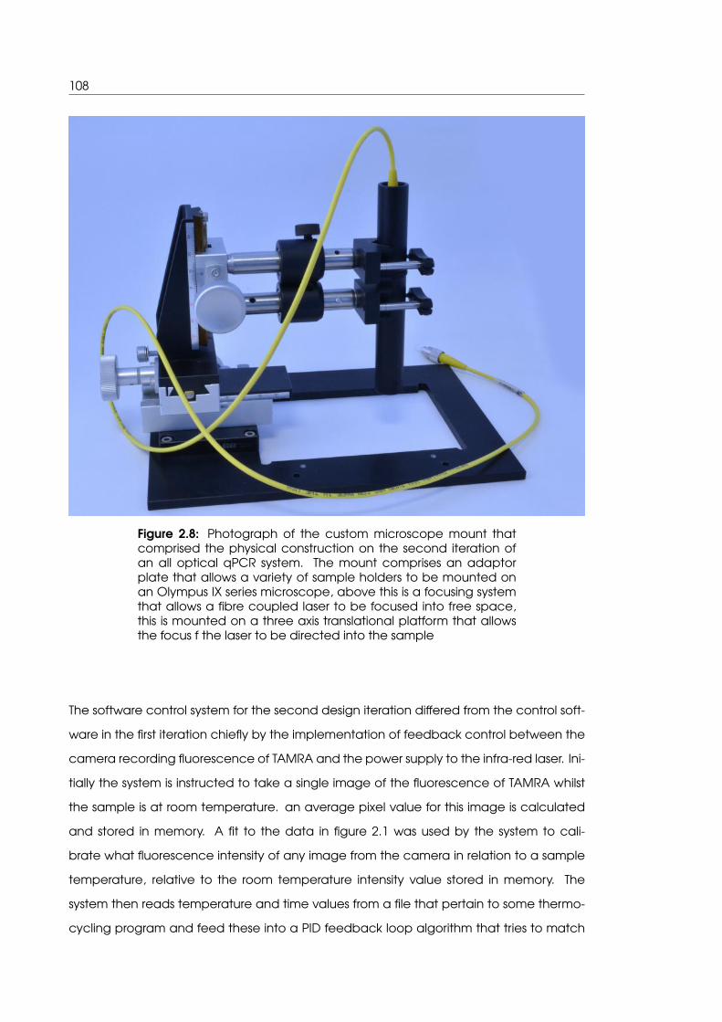
108
Figure 2.8: Photograph of the custom microscope mount thatcomprised the physical construction on the second iteration ofan all optical qPCR system. The mount comprises an adaptorplate that allows a variety of sample holders to be mounted onan Olympus IX series microscope, above this is a focusing systemthat allows a fibre coupled laser to be focused into free space,this is mounted on a three axis translational platform that allowsthe focus f the laser to be directed into the sample
The software control system for the second design iteration differed from the control soft-
ware in the first iteration chiefly by the implementation of feedback control between the
camera recording fluorescence of TAMRA and the power supply to the infra-red laser. Ini-
tially the system is instructed to take a single image of the fluorescence of TAMRA whilst
the sample is at room temperature. an average pixel value for this image is calculated
and stored in memory. A fit to the data in figure 2.1 was used by the system to cali-
brate what fluorescence intensity of any image from the camera in relation to a sample
temperature, relative to the room temperature intensity value stored in memory. The
system then reads temperature and time values from a file that pertain to some thermo-
cycling program and feed these into a PID feedback loop algorithm that tries to match
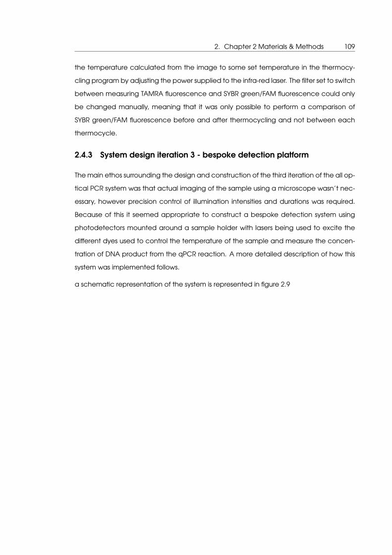
2. Chapter 2 Materials & Methods 109
the temperature calculated from the image to some set temperature in the thermocy-
cling program by adjusting the power supplied to the infra-red laser. The filter set to switch
between measuring TAMRA fluorescence and SYBR green/FAM fluorescence could only
be changed manually, meaning that it was only possible to perform a comparison of
SYBR green/FAM fluorescence before and after thermocycling and not between each
thermocycle.
2.4.3 System design iteration 3 - bespoke detection platform
The main ethos surrounding the design and construction of the third iteration of the all op-
tical PCR system was that actual imaging of the sample using a microscope wasn’t nec-
essary, however precision control of illumination intensities and durations was required.
Because of this it seemed appropriate to construct a bespoke detection system using
photodetectors mounted around a sample holder with lasers being used to excite the
different dyes used to control the temperature of the sample and measure the concen-
tration of DNA product from the qPCR reaction. A more detailed description of how this
system was implemented follows.
a schematic representation of the system is represented in figure 2.9
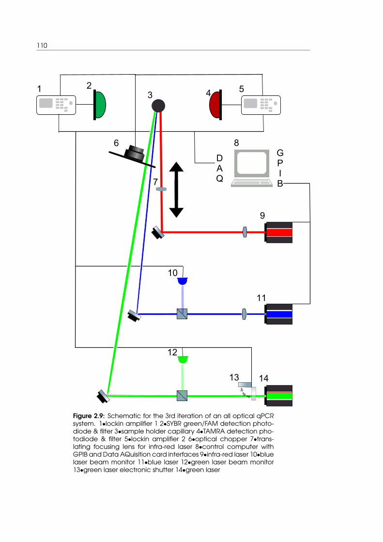
110
GPIB
DAQ
1 23 4 5
6
7
9
11
1413
12
8
10
Figure 2.9: Schematic for the 3rd iteration of an all optical qPCRsystem. 1•lockin amplifier 1 2•SYBR green/FAM detection photo-diode & filter 3•sample holder capillary 4•TAMRA detection pho-todiode & filter 5•lockin amplifier 2 6•optical chopper 7•trans-lating focusing lens for infra-red laser 8•control computer withGPIB and Data AQuisition card interfaces 9•infra-red laser 10•bluelaser beam monitor 11•blue laser 12•green laser beam monitor13•green laser electronic shutter 14•green laser

2. Chapter 2 Materials & Methods 111
The entire system was mounted on a standard optical bench. a protective chassis was
constructed using 25mm aluminium framing with sheet steel walls and a laser curtain on
one side allowing physical access to the system. The overall size of the safety enclosure
was 1.5m by 1m by 50cm, this was manufactured at the Institute of Making, UCL, utilising
a variety of machining techniques. Furthermore a non latching magnetic relay device
was constructed such that multiple lasers could be connected to magnetic door safety
interlock (Lasermet, Bournemouth, UK). A photograph of the entire system is shown in
figure 2.10
Figure 2.10: A picture of the entire setup for the 3rd iteration of anall optical qPCR machine 1| Rail one contains the green laser subsystem 2| contains the blue laser subsystem 3| contains the infrared laser sub system, the optical chopper in in the background4| contains the two detection channels and sample holder sub-system
A green laser system was constructed to cause excitation of the TAMRA in the sample,
a 532nm continuous wave green laser (Altechna ,Vilnius, Lithuania) was mounted to the
optical bench, an electronically controlled 1" diaphragm shutter (Thorlabs) was placed
in the beam path such that the exposure of the sample to the beam could be controlled
programmatically. the beam passed through an optical pick off that directed circa 1% of
the beam into a PDA100A amplified photodetector (Thorlabs) to be used as a beam sta-
112
bility monitor. The beam then strikes and is reflected by an aluminium mirror mounted on
a two-axis kinematic mount (Thorlabs) this enables steering of the beam position in the
plane perpendicular to the direction of travel of the beam where it intersects the sam-
ple. Subsequent to this the beam passed through an optical chopper system (Thorlabs)
a chopper blade was constructed for this system using two MC2F57 chopper blades with
arc shaped slots machined into one using a CNC milling machine, such that they could
be overlaid and shifted radially to effect a reduced duty cycle of laser illumination on
the sample. The chopper was set to operate at 695hz which was 5hz less than the maxi-
mum but was also not a multiple of the 50hz utility frequency. The signal from the chopper
was passed to a lockin amplifier Scitec 410 (Scitec Instruments Ltd., Trowbridge, UK), to
facilitate final signal extraction. Subsequent to the beam hitting the sample and excit-
ing TAMRA, fluorescence was passed through an imaging system of two convex lenses
with focal length and diameter of 40mm. The focused image of the fluorescence passed
through a dielectric longpass filter model number FELH0550 cutting on at 550nm with an
optical density >7 beyond that, in order to exclude light from the excitation beam scat-
tered by the sample. The fluorescence signal was then detected by another PDA100A
amplified photodetector, passed to the lockin amplifier which in turn passed the signal to
be recorded by a computer via a USB-6210 data acquisition card (National Instruments).
A picture of the laser subsystem rail is shown in figure 2.11, whilst the detection subsystem
rail is shown in figure 2.13
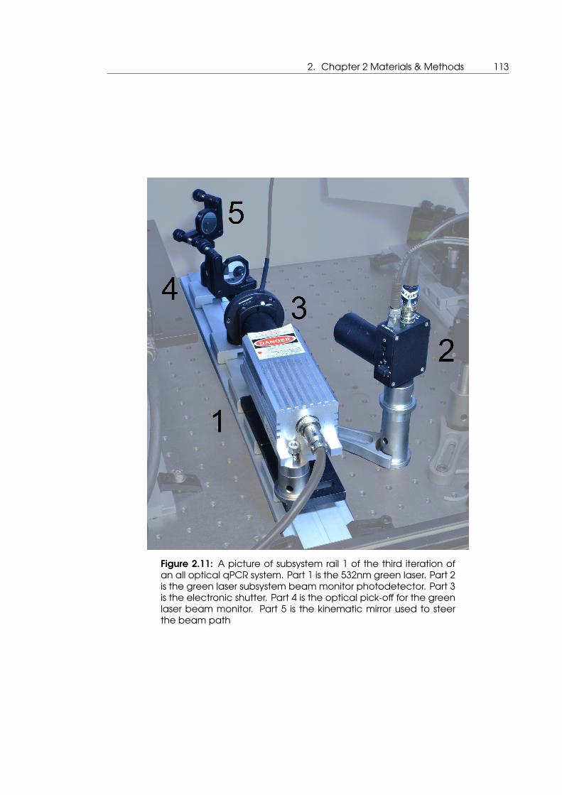
2. Chapter 2 Materials & Methods 113
Figure 2.11: A picture of subsystem rail 1 of the third iteration ofan all optical qPCR system. Part 1 is the 532nm green laser. Part 2is the green laser subsystem beam monitor photodetector. Part 3is the electronic shutter. Part 4 is the optical pick-off for the greenlaser beam monitor. Part 5 is the kinematic mirror used to steerthe beam path

114
A blue laser system was constructed to cause excitation of dyes used to detect DNA con-
centration i.e. SYBR green or FAM. It appeared that continuous lasers in the wavelength
range suitable for this are prohibitively expensive, therefore a home built laser system was
constructed. A PL450B laser diode (OSRAM Licht AG, Munich, Germany) was mated into
a laser diode mount with an integrated thermo-electric cooler (Thorlabs), by the fabri-
cation of a custom copper mounting adaptor, that encapsulated the diode and made
good thermal contact with the thermo-electric cooler by the addition of thermal grease.
a custom lens mount was constructed so that an aspheric lens could be moved towards
the diode for focus control downstream. The thermo-electric cooler was connected to
a model 325 temperature controller (Newport Corporation, Irvine, CA, USA) Power was
supplied to the system using a spare output channel on the HAMEG 2030 power supply.
In this manner the blue laser system can be controlled via GPIB in the same manner as
the infra-red laser system. The beam of the blue laser then followed through the same
arrangement of components as with the green laser system, with the exceptions that a
model 5210 lock in amplifier was used (Princeton Applied Research, Oak Ridge, TN, USA)
and a band pass filter model number FBH520 (Thorlabs) restricting light entering the de-
tector to wavelengths between 500 and 540nm. A picture of this laser subsystem rail is
shown in figure 2.12, whilst the detection subsystem rail is shown in figure 2.13

2. Chapter 2 Materials & Methods 115
Figure 2.12: A picture of subsystem rail 2 of the third iteration ofan all optical qPCR system. Part 1 is the 450nm blue laser, the at-tached temperature regulator and power supply are out of view.Part 2 is the blue laser subsystem beam monitor photodetector.Part 3 is the optical pick-off for the green laser beam monitor. Part4 is the kinematic mirror used to steer the beam path
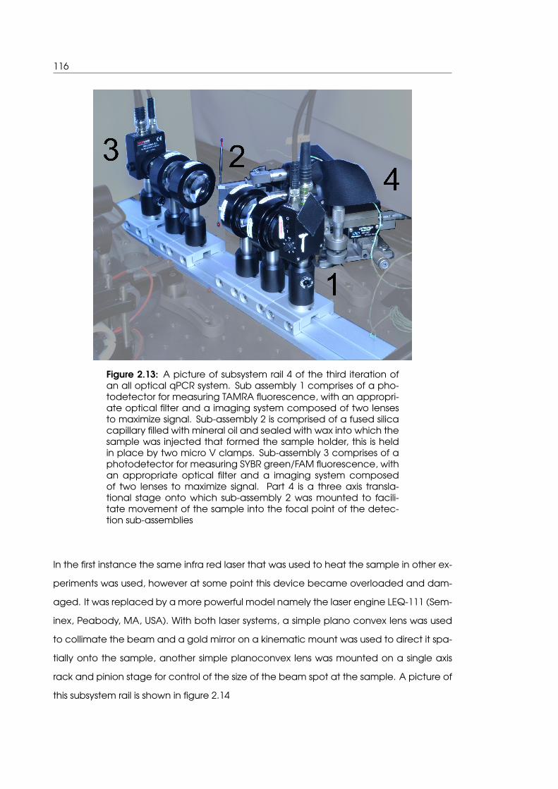
116
Figure 2.13: A picture of subsystem rail 4 of the third iteration ofan all optical qPCR system. Sub assembly 1 comprises of a pho-todetector for measuring TAMRA fluorescence, with an appropri-ate optical filter and a imaging system composed of two lensesto maximize signal. Sub-assembly 2 is comprised of a fused silicacapillary filled with mineral oil and sealed with wax into which thesample was injected that formed the sample holder, this is heldin place by two micro V clamps. Sub-assembly 3 comprises of aphotodetector for measuring SYBR green/FAM fluorescence, withan appropriate optical filter and a imaging system composedof two lenses to maximize signal. Part 4 is a three axis transla-tional stage onto which sub-assembly 2 was mounted to facili-tate movement of the sample into the focal point of the detec-tion sub-assemblies
In the first instance the same infra red laser that was used to heat the sample in other ex-
periments was used, however at some point this device became overloaded and dam-
aged. It was replaced by a more powerful model namely the laser engine LEQ-111 (Sem-
inex, Peabody, MA, USA). With both laser systems, a simple plano convex lens was used
to collimate the beam and a gold mirror on a kinematic mount was used to direct it spa-
tially onto the sample, another simple planoconvex lens was mounted on a single axis
rack and pinion stage for control of the size of the beam spot at the sample. A picture of
this subsystem rail is shown in figure 2.14

2. Chapter 2 Materials & Methods 117
Figure 2.14: A picture of subsystem rail 3 of the third iteration ofan all optical qPCR system. Part 1 is the infra-red laser, here theseminex leq-111 that replaced the previously damaged laser isshown. Part 2 is the collimating lens. Part 3 is the kinematic mirrorused to direct the laser spot at the sample in the place perpen-dicular to the direction of travel. Part 4 is the focusing lens usedto direct the laser spot at the sample in the plane with the direc-tion of the beams travel. Part 5 is the customized optical chopperwheel that is actually part of subsystem rails 1&2 but was physi-cally near rail 3

118
The control software developed in Labview (National Instruments) for the system oper-
ates,in the following manner. The main program loop runs in the background and waits
for a change in state of any of the main system controls. Under normal operation the
system initializes by providing specified voltage and current to the cooling system of the
infra-red laser. It then sets specified voltage values only to the Infra-red and blue lasers.
The shutter of the green laser then opens for 150ms and a room temperature reading for
TAMRA fluorescence is made divided by the intensity reading of the green laser beam
monitor and stored in memory, the shutter is then closed. A PCR program is entered by
the user, which can be saved to or read from a text file. On starting PCR the system will
change the current value supplied to the infra-red laser so that the temperature of the
sample approaches that stated in the PCR program. In order to measure the tempera-
ture the shutter of the green laser is opened and the fluorescence of TAMRA divided by
the beam monitor value relative to the room temperature measurement stored in mem-
ory is compared to the calibration curve shown in figure 2.3. The temperature value and
the current set point stipulated by the PCR program are fed into a software PID controller
to output current values to the infra-red laser. At the end of every thermocycle the shut-
ter of the green laser is closed and a holding current of 600mA is provided to the infra-red
laser, this was determined to be the average current value when the PID was maintaining
a temperature of 60◦C. The blue laser is fired by supplying a specified current value, the
SYBR green/FAM fluorescence divided by the blue laser beam monitor is then recorded
and stored in memory. The green laser shutter is then reopened and temperature reg-
ulation by the PID is restarted as before. When the PCR run has finished all recorded
fluorescence values & calculated values by the PID are written to a text file for later anal-
ysis and all subsystems are put into an idle state. Throughout this entire process all control
signals and measurements sent and received between the various system components
and the computer control software were communicated by the data acquisition card
and the GPIB interface.

3. Chapter 3 Results of Protein stability measurements in nl range 119
3. Chapter 3 Results of Protein stability
measurements in nl range
120
3.1 Introduction to Results of Protein stability measurements
in nl range
A system was implemented to perform measurements of Protein stability measurements
in nl range. This was mediated by performing optical thermometry and heating in a mi-
crofluidic device. These implementation and measurements would form the foundation
of how optical thermo-regulation of a biological system in a microfluidic device can be
used to perform commercially useful measurements
3.2 Imaging of GFP and TAMRA fluorescence to deduce GFP
denaturation as a function of temperature also shows a
time dependence of GFP denaturation
This work was performed in collaboration with Dr. Sagar M Dodderi. Sample preparation
was performed at the Department of Biochemical Engineering University College London,
data acquisition and analysis was performed at the London Centre for Nanotechnology
As was established earlier in the introduction and literature review protein structure dic-
tates protein function. Furthermore measurement of protein stability can give tremen-
dous insights into this structure and function. This can be seen in the drive to understand
and characterize protein folding and aggregation in diseases such as Alzheimer’s and in
measuring biding affinity of drugs to protein targets in the initial phases of a drug devel-
opment pipeline[Pantoliano et al., 2001, Hau et al., 2011].
Furthermore as explored in the introduction, microfluidics facilitates the use of small
sample volumes. This can lead to high throughput assays leading to faster devel-
opment in the aforementioned areas in which protein stability measurements are
key[Gaudet et al., 2010].
With a view to this a microfluidic system was constructed as outlined in the materials and
methods section, by which the stability of GFP was measured as a function of tempera-
ture by monitoring its fluorescence as heating was induced optically.
What follows are the results from these measurements in which by imaging the fluores-
cence of GFP and TAMRA in a microfluidic device the time dependence of the denatu-
3. Chapter 3 Results of Protein stability measurements in nl range 121
ration of GFP as a function of temperature are deduced.
Figure 3.1 shows data gathered over time for both TAMRA and GFP fluorescence where a
infra-red laser heating spot is introduced by providing a level of laser power that was de-
termined to induce unfolding of GFP. The heating spot is at centre point of the plots and
labelled 0µM on the capillary axis. Fluorescence was recorded for both colour chan-
nels every thirty seconds for ten minutes. The temperature along the capillary is deduced
from the temperature sensitive fluorescence of TAMRA described earlier. The plot shows
that TAMRA fluorescence has a time dependence below 30s with a stable gradient of
temperature created along the capillary axis for the ten minute duration of the exper-
iment. The fluorescence of GFP, however, shows a time dependence greater than 30s,
This indicates that this decay in fluorescence is related to the thermal denaturation rate
of GFP, as the drop in fluorescence occurs much more rapidly at closer proximity to the
laser heating spot where the temperature as measured by TAMRA fluorescence is higher
compared to colder areas distal from the laser heating spot.
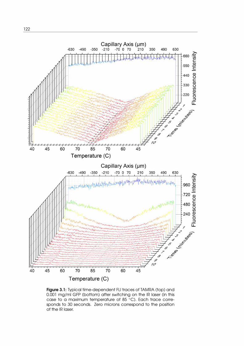
122
Figure 3.1: Typical time-dependent FLI traces of TAMRA (top) and0.001 mg/ml GFP (bottom) after switching on the IR laser (in thiscase to a maximum temperature of 85 ◦C). Each trace corre-sponds to 30 seconds. Zero microns correspond to the positionof the IR laser.
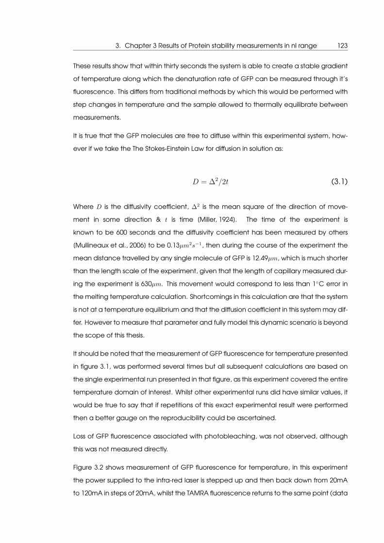
3. Chapter 3 Results of Protein stability measurements in nl range 123
These results show that within thirty seconds the system is able to create a stable gradient
of temperature along which the denaturation rate of GFP can be measured through it’s
fluorescence. This differs from traditional methods by which this would be performed with
step changes in temperature and the sample allowed to thermally equilibrate between
measurements.
It is true that the GFP molecules are free to diffuse within this experimental system, how-
ever if we take the The Stokes-Einstein Law for diffusion in solution as:
D = ∆2/2t (3.1)
Where D is the diffusivity coefficient, ∆2 is the mean square of the direction of move-
ment in some direction & t is time [Miller, 1924]. The time of the experiment is
known to be 600 seconds and the diffusivity coefficient has been measured by others
[Mullineaux et al., 2006] to be 0.13µm2s−1, then during the course of the experiment the
mean distance travelled by any single molecule of GFP is 12.49µm, which is much shorter
than the length scale of the experiment, given that the length of capillary measured dur-
ing the experiment is 630µm. This movement would correspond to less than 1◦C error in
the melting temperature calculation. Shortcomings in this calculation are that the system
is not at a temperature equilibrium and that the diffusion coefficient in this system may dif-
fer. However to measure that parameter and fully model this dynamic scenario is beyond
the scope of this thesis.
It should be noted that the measurement of GFP fluorescence for temperature presented
in figure 3.1, was performed several times but all subsequent calculations are based on
the single experimental run presented in that figure, as this experiment covered the entire
temperature domain of interest. Whilst other experimental runs did have similar values, it
would be true to say that if repetitions of this exact experimental result were performed
then a better gauge on the reproducibility could be ascertained.
Loss of GFP fluorescence associated with photobleaching, was not observed, although
this was not measured directly.
Figure 3.2 shows measurement of GFP fluorescence for temperature, in this experiment
the power supplied to the infra-red laser is stepped up and then back down from 20mA
to 120mA in steps of 20mA, whilst the TAMRA fluorescence returns to the same point (data
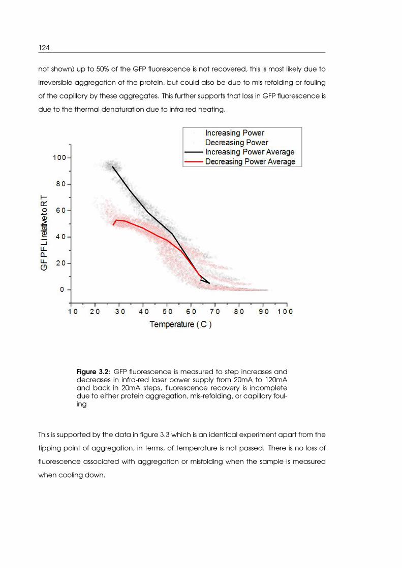
124
not shown) up to 50% of the GFP fluorescence is not recovered, this is most likely due to
irreversible aggregation of the protein, but could also be due to mis-refolding or fouling
of the capillary by these aggregates. This further supports that loss in GFP fluorescence is
due to the thermal denaturation due to infra red heating.
Figure 3.2: GFP fluorescence is measured to step increases anddecreases in infra-red laser power supply from 20mA to 120mAand back in 20mA steps, fluorescence recovery is incompletedue to either protein aggregation, mis-refolding, or capillary foul-ing
This is supported by the data in figure 3.3 which is an identical experiment apart from the
tipping point of aggregation, in terms, of temperature is not passed. There is no loss of
fluorescence associated with aggregation or misfolding when the sample is measured
when cooling down.
3. Chapter 3 Results of Protein stability measurements in nl range 125
Figure 3.3: GFP fluorescence is measured to step increases anddecreases in infra-red laser power supply from 20mA to 120mAand back in 20mA steps, fluorescence is not lost as the tippingpoint of aggregation has not been passed
3.3 Calculation of GFP denaturation from fluorescence signal
decay rate
The fluorescence of TAMRA and GFP both fall as the temperature increases dues to heat-
ing by the infra-red laser. As these drops are symmetrical the fluorescence of TAMRA for a
point (on either side of the laser spot) is used to calculate the temperature at that point,
and the GFP fluorescence measurements gated out into 5◦C sections, this is then plotted
versus time as seen in the top portion of figure 3.4
The fluorescence values are normalized to a room temperature fluorescence value with
the key point obvious from the plot that the rate of decrease of fluorescence is slower
at lower temperatures, i.e. the locations furthest away from the laser heating spot. With
these time dependent GFP fluorescence decay curves obtained from 46◦C to 85◦C they
are fit to equation 3.2 to give k which is the rate constant of GFP denaturation as a

126
function of temperature and where where a is the measured signal amplitude and c is
the fluorescence signal decay end point. The logarithm of these rate constants versus
temperature are shown on the lower plot of figure 3.4.
y = a exp (−kt) + c (3.2)
The logarithm of the rate constants changes in a non linear manner for change in tem-
perature. This be roughly generalized to two separate linear regimes where the change
in the slope occurs at 60◦C, indicating a change from purely reversible unfolding of GFP
to a situation where non-reversible unfolding due to protein aggregation is occurring.

3. Chapter 3 Results of Protein stability measurements in nl range 127
Figure 3.4: Top: GFP denaturation decay curves at selected tem-peratures from 46–81◦C obtained by fluorescence image scan-ning at 30 s intervals for a single IR-heated capillary region. Lineswere best fit to equation 3.2 , and shown at 46◦C (red), 49◦C (darkyellow), 51.5◦C (cyan), 54◦C (blue), 56.5◦C (green), 60.5◦C (pink),65◦C (dark green), 69.5◦C (dark blue), 74.5◦C (dark pink), 81◦C(grey). Bottom: Temperature dependence of the logarithm ofthe rate constant, log(ku), of GFP denaturation, obtained usingthe optical heating method, and fitting decay data to Eq. 1.
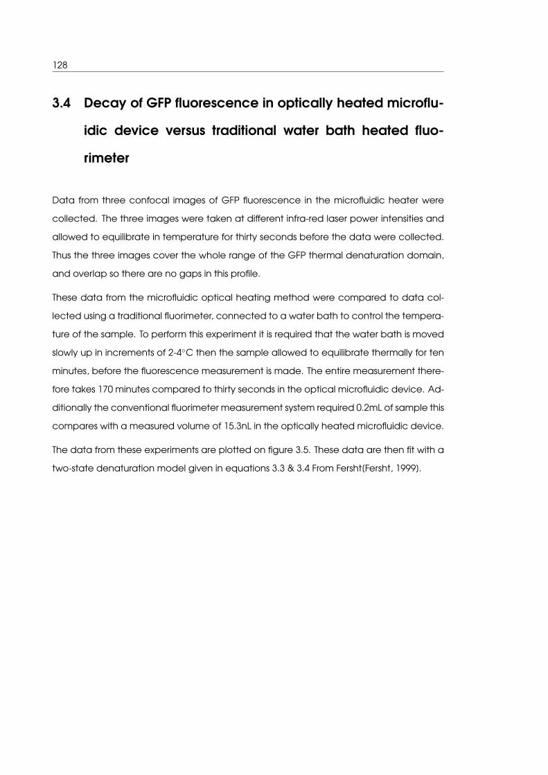
128
3.4 Decay of GFP fluorescence in optically heated microflu-
idic device versus traditional water bath heated fluo-
rimeter
Data from three confocal images of GFP fluorescence in the microfluidic heater were
collected. The three images were taken at different infra-red laser power intensities and
allowed to equilibrate in temperature for thirty seconds before the data were collected.
Thus the three images cover the whole range of the GFP thermal denaturation domain,
and overlap so there are no gaps in this profile.
These data from the microfluidic optical heating method were compared to data col-
lected using a traditional fluorimeter, connected to a water bath to control the tempera-
ture of the sample. To perform this experiment it is required that the water bath is moved
slowly up in increments of 2-4◦C then the sample allowed to equilibrate thermally for ten
minutes, before the fluorescence measurement is made. The entire measurement there-
fore takes 170 minutes compared to thirty seconds in the optical microfluidic device. Ad-
ditionally the conventional fluorimeter measurement system required 0.2mL of sample this
compares with a measured volume of 15.3nL in the optically heated microfluidic device.
The data from these experiments are plotted on figure 3.5. These data are then fit with a
two-state denaturation model given in equations 3.3 & 3.4 From Fersht[Fersht, 1999].
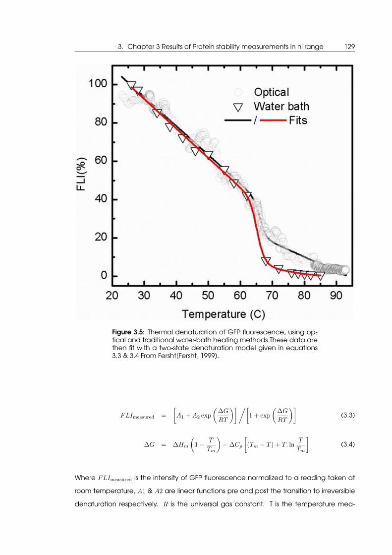
3. Chapter 3 Results of Protein stability measurements in nl range 129
Figure 3.5: Thermal denaturation of GFP fluorescence, using op-tical and traditional water-bath heating methods These data arethen fit with a two-state denaturation model given in equations3.3 & 3.4 From Fersht[Fersht, 1999].
FLImeasured =
[A1 +A2 exp
(∆G
RT
)]/[1 + exp
(∆G
RT
)](3.3)
∆G = ∆Hm
(1− T
Tm
)−∆Cp
[(Tm − T ) + T. ln
T
Tm
](3.4)
Where FLImeasured is the intensity of GFP fluorescence normalized to a reading taken at
room temperature, A1 & A2 are linear functions pre and post the transition to irreversible
denaturation respectively. R is the universal gas constant. T is the temperature mea-
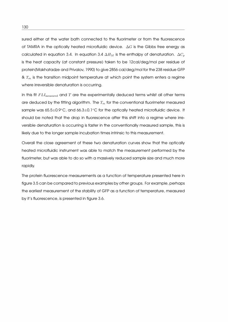
130
sured either at the water bath connected to the fluorimeter or from the fluorescence
of TAMRA in the optically heated microfluidic device. ∆G is the Gibbs free energy as
calculated in equation 3.4. In equation 3.4 ∆HM is the enthalpy of denaturation. ∆Cp
is the heat capacity (at constant pressure) taken to be 12cal/deg/mol per residue of
protein[Makhatadze and Privalov, 1990] to give 2856 cal/deg/mol for the 238 residue GFP
& Tm is the transition midpoint temperature at which point the system enters a regime
where irreversible denaturation is occurring.
In this fit FLImeasured and T are the experimentally deduced terms whilst all other terms
are deduced by the fitting algorithm. The Tm for the conventional fluorimeter measured
sample was 65.5±0.9◦C, and 66.3±0.1◦C for the optically heated microfluidic device. It
should be noted that the drop in fluorescence after this shift into a regime where irre-
versible denaturation is occurring is faster in the conventionally measured sample, this is
likely due to the longer sample incubation times intrinsic to this measurement.
Overall the close agreement of these two denaturation curves show that the optically
heated microfluidic instrument was able to match the measurement performed by the
fluorimeter, but was able to do so with a massively reduced sample size and much more
rapidly.
The protein fluorescence measurements as a function of temperature presented here in
figure 3.5 can be compared to previous examples by other groups. For example, perhaps
the earliest measurement of the stability of GFP as a function of temperature, measured
by it’s fluorescence, is presented in figure 3.6.

3. Chapter 3 Results of Protein stability measurements in nl range 131
Figure 3.6: A measurement of GFP fluorescence measured as afunction of temperature from [Bokman and Ward, 1981] used togauge the thermal stability of the protein, the solid dots indicatesmeasurement of the sample where only heat has been used asa denaturant, all other data points should be disregarded.
There are some differences from the measurement shown in figures 3.5 & 3.6, these are
due to differences in the measurement procedure and samples used. In the measure-
ment by Bokman and Ward in 1981, the sample was heated to each temperature point
in the range, and then cooled to room temperature, before the fluorescence was mea-
sured. This differs from the measurements in figure 3.5 in which the sample is actually
measured at the temperature point presented. This means that the fluorescence of the
sample is affected by temperature before & after denaturation occurs. That effect ac-
counts for the linear declines in fluorescence observed, both prior and post denaturation
of the protein, in the optical & water bath heating methods shown in figure 3.5. Addition-
ally the temperature point at which the transition to a denaturing regime occurs differs
for the two plots. This is due to different mutants of GFP being used as the test sample, as
well as differences in the buffering conditions.
Another example of a measurement of GFP fluorescence measured as a function of
temperature is shown in figure 3.7.

132
Figure 3.7: A measurement of GFP fluorescence measured asa function of temperature from iGEM Part:BBa_K515105 used togauge the thermal stability of the protein. The light green plot isthe sample most similar to that of the one presented in this thesis.
This differs from the measurements presented in figure 3.5 in the same manner as the Bok-
man & Ward measurements, in that the actual fluorescence measurement is performed
at room temperature. However the temperature point at which the transition to denat-
uration occurs, is more similar than in the Bokman & Ward measurements, presumably
because the mutant of GFP and buffering conditions used are more similar to those of
the measurements presented in this thesis.
Whilst it is true that there are differences between the few examples that exist in the lit-
erature of measurements of GFP fluorescence as a function of temperature, and those
presented in this thesis, there is close agreement in the measurements taken in the novel
infra-red laser heated setup, and the traditionally heated water-bath based control ex-
periment.

4. Chapter 4 Results of HBV sequencing 133
4. Chapter 4 Results of HBV sequencing

134
4.1 Introduction to results of HBV sequencing
A variety of DNA sequencing experiments were performed of people undergoing treat-
ment in a clinical setting. These results would be used as a test case, against which the
development of an all optical qPCR device would be tested. Using a clinical test case
would such as this would give the development of such a system much greater relevance.
4.2 Results of Sanger sequencing
The qPCR and Sanger sequencing work was largely performed by Dr. Antonio Adrián
González del Castillo, with my assistance, using the protocols in place at the Royal Free
Hospital, Department of Virology, London. Statistical analysis was performed with Prof.
Anna Maria Geretti, at the University of Liverpool. These results are presented here as
they form the background of the other sequencing analyses performed by me and de-
tailed later.
Start + 6 Months +12 Months
Total numberattending 133(100%) 96(100%) 54(100%)
Hbe antigen positive 67(50.4%) 45(47%) 24(44.4%)
HBV DNA >12 IU/ml, n(%) 124(93%) 57(59%) 20(37%)
HBV DNA >2000 IU/ml, n (%) 99(74.4%) 24(25%) 18(33.3%)
Sanger sequences, n (%) 111(85%) 40(41.7%) 19(35.2%)
Mutation detected, n (%) 0(0%) 8(8.3%) 18(33.3%)
M204I/M 0(0%) 8(8.3%) 0(0%)
M204V L180M 0 0 10
M204V V173L L180M 0 0 4
M204V L180M A181S 0 0 2
M204V L80I 0 0 1
M204V L80I L180M 0 0 1
Table 4.1: Table of results of Sanger sequencing of Malawi cohort
Patients who presented to the Queen Elizabeth Central Hospital (QECH) of Blantyre,
Malawi, with suspected HIV in 2007-2009 were eligible to start a fixed dose treatment
regimen containing Stavudine Lamivudine Nevirapine. Indications for starting the treat-
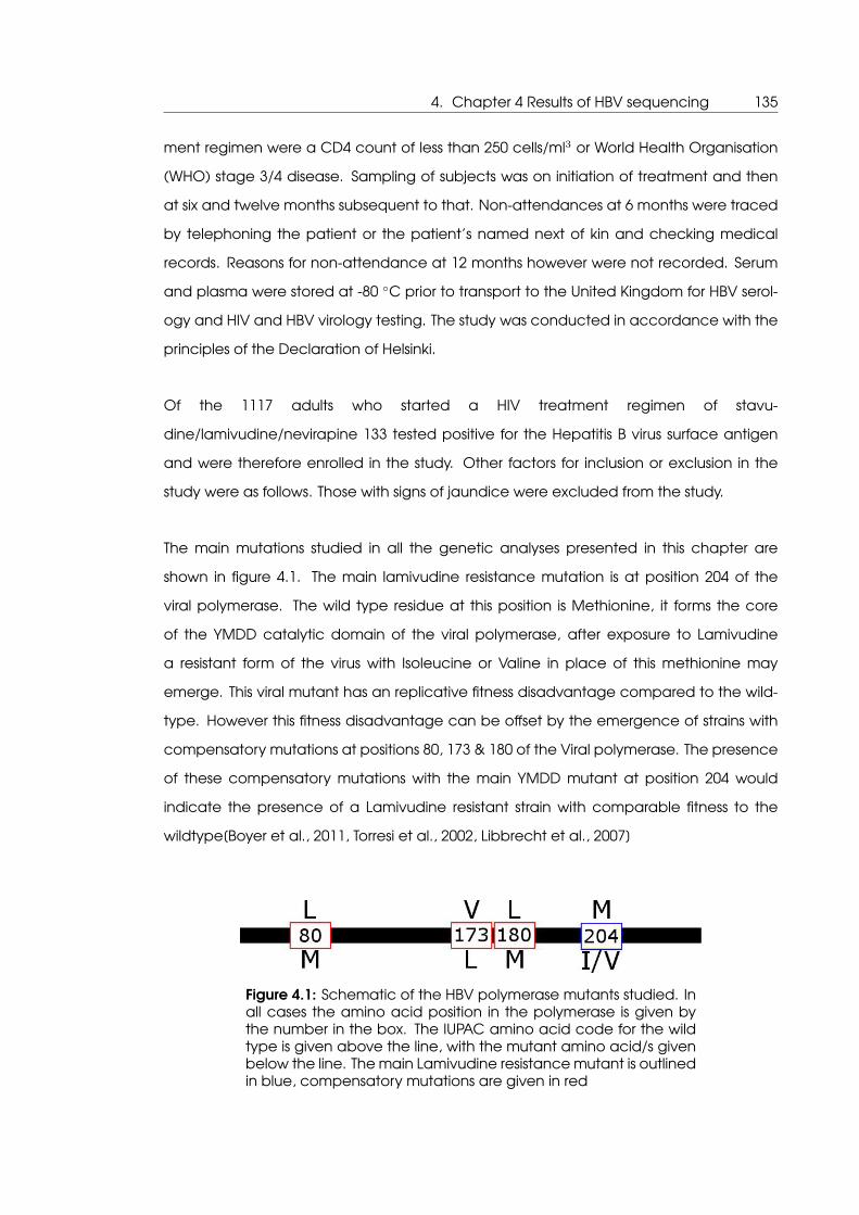
4. Chapter 4 Results of HBV sequencing 135
ment regimen were a CD4 count of less than 250 cells/ml3 or World Health Organisation
(WHO) stage 3/4 disease. Sampling of subjects was on initiation of treatment and then
at six and twelve months subsequent to that. Non-attendances at 6 months were traced
by telephoning the patient or the patient’s named next of kin and checking medical
records. Reasons for non-attendance at 12 months however were not recorded. Serum
and plasma were stored at -80 ◦C prior to transport to the United Kingdom for HBV serol-
ogy and HIV and HBV virology testing. The study was conducted in accordance with the
principles of the Declaration of Helsinki.
Of the 1117 adults who started a HIV treatment regimen of stavu-
dine/lamivudine/nevirapine 133 tested positive for the Hepatitis B virus surface antigen
and were therefore enrolled in the study. Other factors for inclusion or exclusion in the
study were as follows. Those with signs of jaundice were excluded from the study.
The main mutations studied in all the genetic analyses presented in this chapter are
shown in figure 4.1. The main lamivudine resistance mutation is at position 204 of the
viral polymerase. The wild type residue at this position is Methionine, it forms the core
of the YMDD catalytic domain of the viral polymerase, after exposure to Lamivudine
a resistant form of the virus with Isoleucine or Valine in place of this methionine may
emerge. This viral mutant has an replicative fitness disadvantage compared to the wild-
type. However this fitness disadvantage can be offset by the emergence of strains with
compensatory mutations at positions 80, 173 & 180 of the Viral polymerase. The presence
of these compensatory mutations with the main YMDD mutant at position 204 would
indicate the presence of a Lamivudine resistant strain with comparable fitness to the
wildtype[Boyer et al., 2011, Torresi et al., 2002, Libbrecht et al., 2007]
Figure 4.1: Schematic of the HBV polymerase mutants studied. Inall cases the amino acid position in the polymerase is given bythe number in the box. The IUPAC amino acid code for the wildtype is given above the line, with the mutant amino acid/s givenbelow the line. The main Lamivudine resistance mutant is outlinedin blue, compensatory mutations are given in red
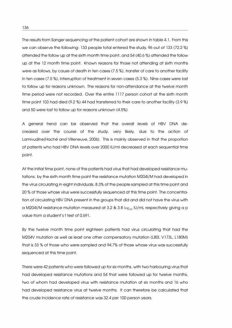
136
The results from Sanger sequencing of the patient cohort are shown in table 4.1. From this
we can observe the following: 133 people total entered the study, 96 out of 133 (72.2 %)
attended the follow up at the sixth month time point, and 54 (40.6 %) attended the follow
up at the 12 month time point. Known reasons for those not attending at sixth months
were as follows, by cause of death in ten cases (7.5 %), transfer of care to another facility
in ten cases (7.5 %), interruption of treatment in seven cases (5.3 %). Nine cases were lost
to follow up for reasons unknown. The reasons for non-attendance at the twelve month
time period were not recorded. Over the entire 1117 person cohort at the sixth month
time point 103 had died (9.2 %) 44 had transferred to their care to another facility (3.9 %)
and 50 were lost to follow up for reasons unknown (4.5%)
A general trend can be observed that the overall levels of HBV DNA de-
creased over the course of the study, very likely, due to the action of
Lamivudine[Haché and Villeneuve, 2006]. This is mainly observed in that the proportion
of patients who had HBV DNA levels over 2000 IU/ml decreased at each sequential time
point.
At the initial time point, none of the patients had virus that had developed resistance mu-
tations. by the sixth month time point the resistance mutation M204I/M had developed in
the virus circulating in eight individuals, 8.3% of the people sampled at this time point and
20 % of those whose virus were successfully sequenced at this time point. The concentra-
tion of circulating HBV DNA present in the groups that did and did not have the virus with
a M204I/M resistance mutation measured at 3.2 & 3.8 log10 IU/mL respectively giving a p
value from a student’s t test of 0.691.
By the twelve month time point eighteen patients had virus circulating that had the
M204V mutation as well as least one other compensatory mutation (L80I, V173L, L180M)
that is 33 % of those who were sampled and 94.7% of those whose virus was successfully
sequenced at this time point.
There were 42 patients who were followed up for six months, with two harbouring virus that
had developed resistance mutations and 54 that were followed up for twelve months,
two of whom had developed virus with resistance mutation at six months and 16 who
had developed resistance virus at twelve months. It can therefore be calculated that
the crude incidence rate of resistance was 32.4 per 100 person years.

4. Chapter 4 Results of HBV sequencing 137
4.3 Next generation Sequencing of HBV mutants by ’454’
deep sequencing
This work here of amplicon production was performed largely at the Royal Free Hospi-
tal Department of Virology, London. Amplicon balancing which was performed at the
Rayne Institute, University College London. This work was performed without any col-
laboration, however, Dr. Ian Harrison provided useful discussion with regards to the op-
timization of the protocol. The sequencing reactions were performed at the Centre for
Genomic Research University of Liverpool. Here useful discussions were had with Dr. John
Kenny with regards to how the sequencing reactions should be set up.
The results of the first deep sequencing experiment using the ’454’ deep sequencing
platform are presented in tables 4.3& 4.5. These tables list, in each case, the library name,
which is a reference to the unique patient identifier code. M, I & V represent the amino
acid residue that may be present at some residue where M is Methionine, I is Isoleucine,
L is Leucine & V is Valine. The numbers 204, 180 & 173 represent the amino acid position
in the polymerase of HBV where a resistance mutation may be present. The data are
the number of reads that occurred at one of the positions with one of the stated amino
acids.
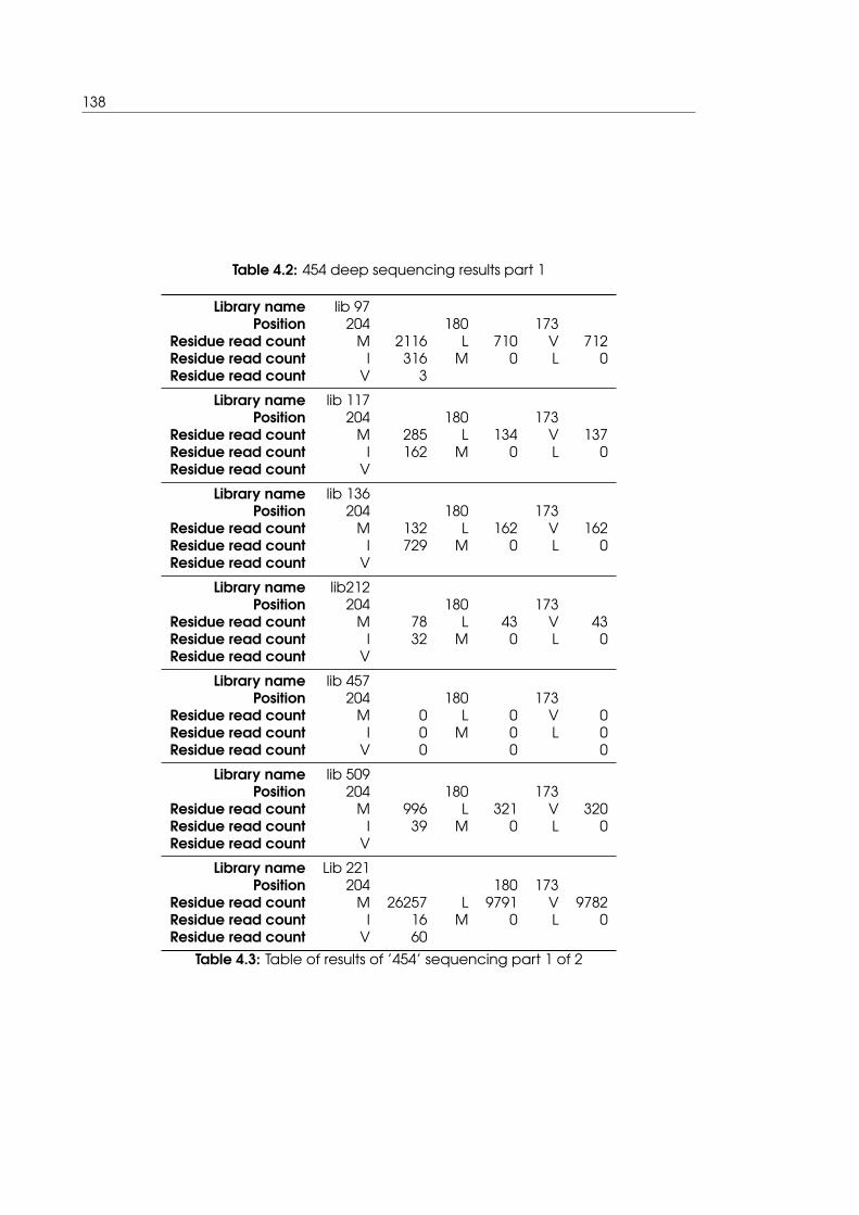
138
Table 4.2: 454 deep sequencing results part 1
Library name lib 97Position 204 180 173
Residue read count M 2116 L 710 V 712Residue read count I 316 M 0 L 0Residue read count V 3
Library name lib 117Position 204 180 173
Residue read count M 285 L 134 V 137Residue read count I 162 M 0 L 0Residue read count V
Library name lib 136Position 204 180 173
Residue read count M 132 L 162 V 162Residue read count I 729 M 0 L 0Residue read count V
Library name lib212Position 204 180 173
Residue read count M 78 L 43 V 43Residue read count I 32 M 0 L 0Residue read count V
Library name lib 457Position 204 180 173
Residue read count M 0 L 0 V 0Residue read count I 0 M 0 L 0Residue read count V 0 0 0
Library name lib 509Position 204 180 173
Residue read count M 996 L 321 V 320Residue read count I 39 M 0 L 0Residue read count V
Library name Lib 221Position 204 180 173
Residue read count M 26257 L 9791 V 9782Residue read count I 16 M 0 L 0Residue read count V 60
Table 4.3: Table of results of ’454’ sequencing part 1 of 2
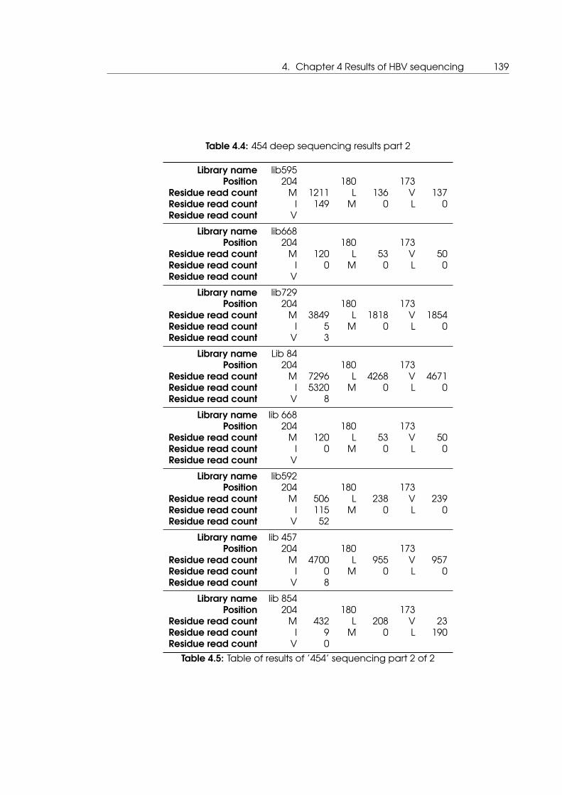
4. Chapter 4 Results of HBV sequencing 139
Table 4.4: 454 deep sequencing results part 2
Library name lib595Position 204 180 173
Residue read count M 1211 L 136 V 137Residue read count I 149 M 0 L 0Residue read count V
Library name lib668Position 204 180 173
Residue read count M 120 L 53 V 50Residue read count I 0 M 0 L 0Residue read count V
Library name lib729Position 204 180 173
Residue read count M 3849 L 1818 V 1854Residue read count I 5 M 0 L 0Residue read count V 3
Library name Lib 84Position 204 180 173
Residue read count M 7296 L 4268 V 4671Residue read count I 5320 M 0 L 0Residue read count V 8
Library name lib 668Position 204 180 173
Residue read count M 120 L 53 V 50Residue read count I 0 M 0 L 0Residue read count V
Library name lib592Position 204 180 173
Residue read count M 506 L 238 V 239Residue read count I 115 M 0 L 0Residue read count V 52
Library name lib 457Position 204 180 173
Residue read count M 4700 L 955 V 957Residue read count I 0 M 0 L 0Residue read count V 8
Library name lib 854Position 204 180 173
Residue read count M 432 L 208 V 23Residue read count I 9 M 0 L 190Residue read count V 0
Table 4.5: Table of results of ’454’ sequencing part 2 of 2
140
In three patients (identifiers 221, 457 and 854) no drug-resistance mutations in the virus
populations they were harbouring were detected. This was in agreement with the re-
sults obtained at the week sixth month timepoint by Sanger sequencing. In two patients
(identifiers 136 and 84), the mutations detected in the viral populations by ’454’ deep
sequencing were those also observed by Sanger sequencing. patient
In 6 patients (identifiers 97, 509, 117, 212, 592, 595) ’454’ deep sequencing detected muta-
tions not observed by population sequencing. The frequency of the mutations detected
only by next-generation sequencing in the cases of patients 97, 509 & 212 involved the
detection of a minority of Isoleucine at position 204 where population sequencing had
only detected Methionine. In patients 221 & 592 a minority of Valine was detected at
position 204 where population sequencing had only detected Methionine or additionally
Isoleucine in the case of patient 592. In patient 595 population sequencing had detected
only Valine at position 204 whereas second generation sequencing detected only a mi-
nority of Isoleucine mutant type. This shows that the deep reading capability of the ’454’
sequencing platform is able to deduce mutant viral sub-populations within individuals
below the detection limit of traditional Sanger sequencing. For patient 854 at position
173, ’454’ deep sequencing recorded a majority Leucine rather than the wild type Valine
shown by Sanger sequencing, this is shown graphically in figure 4.2.
Figure 4.2: Pie chart representing the amino acid residues presentat position 173 of the reverse transcriptase of HBV as elucidatedby ’454’ deep sequencing for the the sample derived from pa-tient 854
Unexpectedly, two samples (668 and 729) showed mutations by population sequencing
but not by next generation sequencing. This indicates that although next generation
sequencing might have a greater sensitivity it might also be subject to preferential ampli-
fication or bias.
There were corresponding changes in the overlapping reading frame of the surface pro-
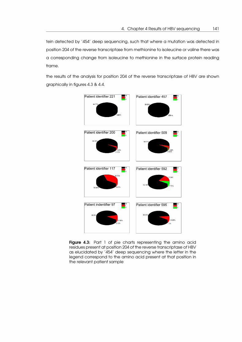
4. Chapter 4 Results of HBV sequencing 141
tein detected by ’454’ deep sequencing, such that where a mutation was detected in
position 204 of the reverse transcriptase from methionine to isoleucine or valine there was
a corresponding change from isoleucine to methionine in the surface protein reading
frame.
the results of the analysis for position 204 of the reverse transcriptase of HBV are shown
graphically in figures 4.3 & 4.4.
Figure 4.3: Part 1 of pie charts representing the amino acidresidues present at position 204 of the reverse transcriptase of HBVas elucidated by ’454’ deep sequencing where the letter in thelegend correspond to the amino acid present at that position inthe relevant patient sample
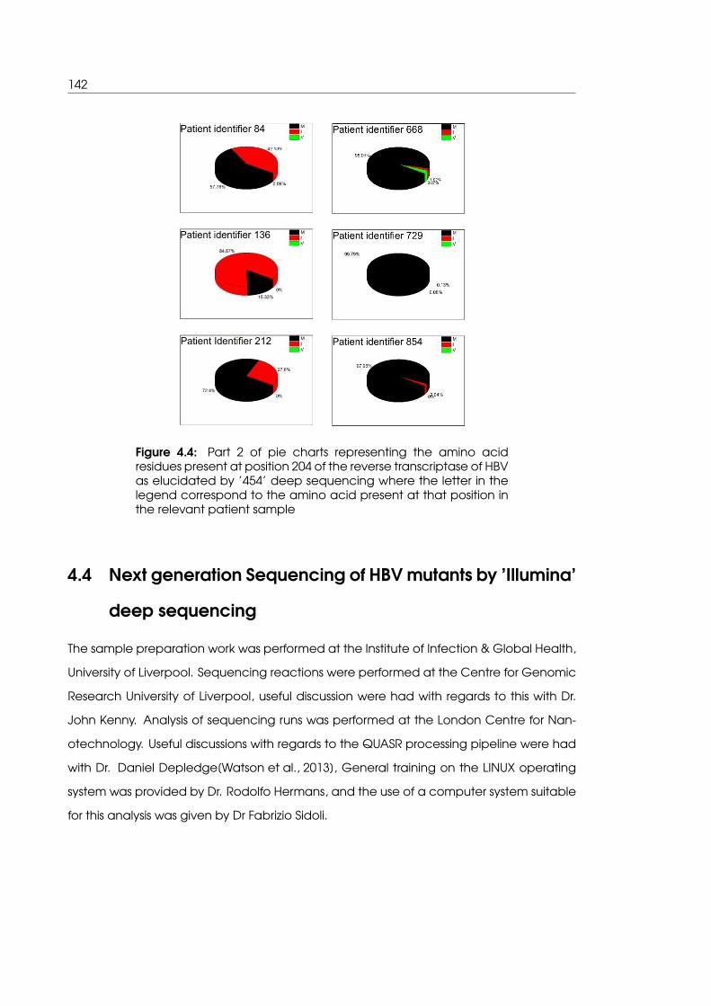
142
Figure 4.4: Part 2 of pie charts representing the amino acidresidues present at position 204 of the reverse transcriptase of HBVas elucidated by ’454’ deep sequencing where the letter in thelegend correspond to the amino acid present at that position inthe relevant patient sample
4.4 Next generation Sequencing of HBV mutants by ’Illumina’
deep sequencing
The sample preparation work was performed at the Institute of Infection & Global Health,
University of Liverpool. Sequencing reactions were performed at the Centre for Genomic
Research University of Liverpool, useful discussion were had with regards to this with Dr.
John Kenny. Analysis of sequencing runs was performed at the London Centre for Nan-
otechnology. Useful discussions with regards to the QUASR processing pipeline were had
with Dr. Daniel Depledge[Watson et al., 2013], General training on the LINUX operating
system was provided by Dr. Rodolfo Hermans, and the use of a computer system suitable
for this analysis was given by Dr Fabrizio Sidoli.
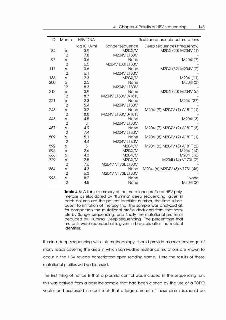
4. Chapter 4 Results of HBV sequencing 143
ID Month HBV DNA Resistance-associated mutations
log10 IU/ml Sanger sequence Deep sequences (frequency)84 6 3.9 M204I/M M204I (20) M204V (1)
12 7.8 M204V L180M -97 6 3.6 None M204I (7)
12 6.5 M204V L80I L180M -117 6 3.6 None M204I (32) M204V (2)
12 6.1 M204V L180M -136 6 2.3 M204I/M M204I (11)200 6 2.5 None M204I (3)
12 8.3 M204V L180M -212 6 3.9 None M204I (20) M204V (6)
12 8.7 M204V L180M A181S -221 6 2.3 None M204I (27)
12 5.4 M204V L180M -243 6 3.2 None M204I (9) M204V (1) A181T (1)
12 8.8 M204V L180M A181S -448 6 4.5 None M204I (3)
12 8 M204V L180M -457 6 4.9 None M204I (7) M204V (2) A181T (3)
12 7.4 M204V L180M -509 6 5.1 None M204I (8) M204V (2) A181T (1)
12 4.4 M204V L180M -592 6 5 M204I/M M204I (6) M204V (3) A181T (2)595 6 2.6 M204I/M M204I (14)668 6 4.3 M204I/M M204I (16)729 6 2.5 M204I/M M204I (14) V173L (2)
12 7.6 M204V V173L L180M -854 6 4.3 None M204I (6) M204V (3) V173L (46)
12 6.3 M204V V173L L180M -996 6 8.2 None None
12 4.8 None M204I (2)
Table 4.6: A table summary of the mutational profile of HBV poly-merase as elucidated by ’Illumina’ deep sequencing, given ineach column are the patient identifier number, the time subse-quent to imitation of therapy that the sample was analyzed at,for comparison the mutational profile deduced from that sam-ple by Sanger sequencing, and finally the mutational profile asdeduced by ’Illumina’ Deep sequencing. The percentage thatmutants were recorded at is given in brackets after the mutantidentifier.
Illumina deep sequencing with this methodology, should provide massive coverage of
many reads covering the area in which Lamivudine resistance mutations are known to
occur in the HBV reverse transcriptase open reading frame. Here the results of these
mutational profiles will be discussed.
The first thing of notice is that a plasmid control was included in the sequencing run,
this was derived from a baseline sample that had been cloned by the use of a TOPO
vector and expressed in e.coli such that a large amount of these plasmids should be

144
entirely homogeneous. The results of the deep sequencing of this plasmid sample at
position 204 of the reverse transcriptase of HBV can be seen in figure 4.6 at the bottom
centre. As expected the majority residue at this position at this timepoint is Methionine,
the minority Valine and Isoleucine are measured 0.17% & 0.03% respectively, this can be
assumed to be be the noise present in the measurement system and therefore a cutoff
of 1% was set up, such that any minority variant detected below this level was assumed
to be artefactual. Other amino acid proportions measured at this position for the plasmid
control were Leucine at 0.07% and Arginine at 0.007%. These measurements lead further
support that in setting a cut off of 1% system noise would be eliminated from the eventual
analysis.
Figure 4.5: Part one of graphical representation of the proteinresidues found a position 204 of the reverse transcriptase of HBVas elucidated by ’Illumina’ deep sequencing. all samples shownare from the sixth month post treatment initiation timepoint
A number of patient samples from the first time point i.e. at initiation of therapy were in-
cluded in this analysis, these were derived from the following patients: 84, 136, 592, 595
& 729, these samples at this time point were included to assess whether ’Illumina’ deep
sequencing could detect any underlying low level resistance populations that exist prior
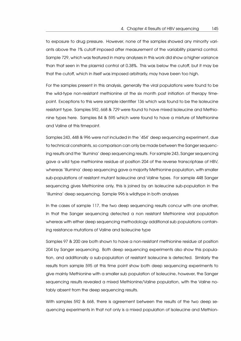
4. Chapter 4 Results of HBV sequencing 145
to exposure to drug pressure. However, none of the samples showed any minority vari-
ants above the 1% cutoff imposed after measurement of the variability plasmid control.
Sample 729, which was featured in many analyses in this work did show a higher variance
than that seen in the plasmid control at 0.38%. This was below the cutoff, but it may be
that the cutoff, which in itself was imposed arbitrarily, may have been too high.
For the samples present in this analysis, generally the viral populations were found to be
the wild-type non-resistant methionine at the six month post initiation of therapy time-
point. Exceptions to this were sample identifier 136 which was found to be the Isoleucine
resistant type. Samples 592, 668 & 729 were found to have mixed Isoleucine and Methio-
nine types here. Samples 84 & 595 which were found to have a mixture of Methionine
and Valine at this timepoint.
Samples 243, 448 & 996 were not included in the ’454’ deep sequencing experiment, due
to technical constraints, so comparison can only be made between the Sanger sequenc-
ing results and the ’Illumina’ deep sequencing results. For sample 243, Sanger sequencing
gave a wild type methionine residue at position 204 of the reverse transcriptase of HBV,
whereas ’Illumina’ deep sequencing gave a majority Methionine population, with smaller
sub-populations of resistant mutant Isoleucine and Valine types. For sample 448 Sanger
sequencing gives Methionine only, this is joined by an Isoleucine sub-population in the
’Illumina’ deep sequencing. Sample 996 is wildtype in both analyses
In the cases of sample 117, the two deep sequencing results concur with one another,
in that the Sanger sequencing detected a non resistant Methionine viral population
whereas with either deep sequencing methodology additional sub populations contain-
ing resistance mutations of Valine and Isoleucine type
Samples 97 & 200 are both shown to have a non-resistant methionine residue at position
204 by Sanger sequencing. Both deep sequencing experiments also show this popula-
tion, and additionally a sub-population of resistant Isoleucine is detected. Similarly the
results from sample 595 at this time point show both deep sequencing experiments to
give mainly Methionine with a smaller sub population of Isoleucine, however, the Sanger
sequencing results revealed a mixed Methionine/Valine population, with the Valine no-
tably absent from the deep sequencing results.
With samples 592 & 668, there is agreement between the results of the two deep se-
quencing experiments in that not only is a mixed population of Isoleucine and Methion-
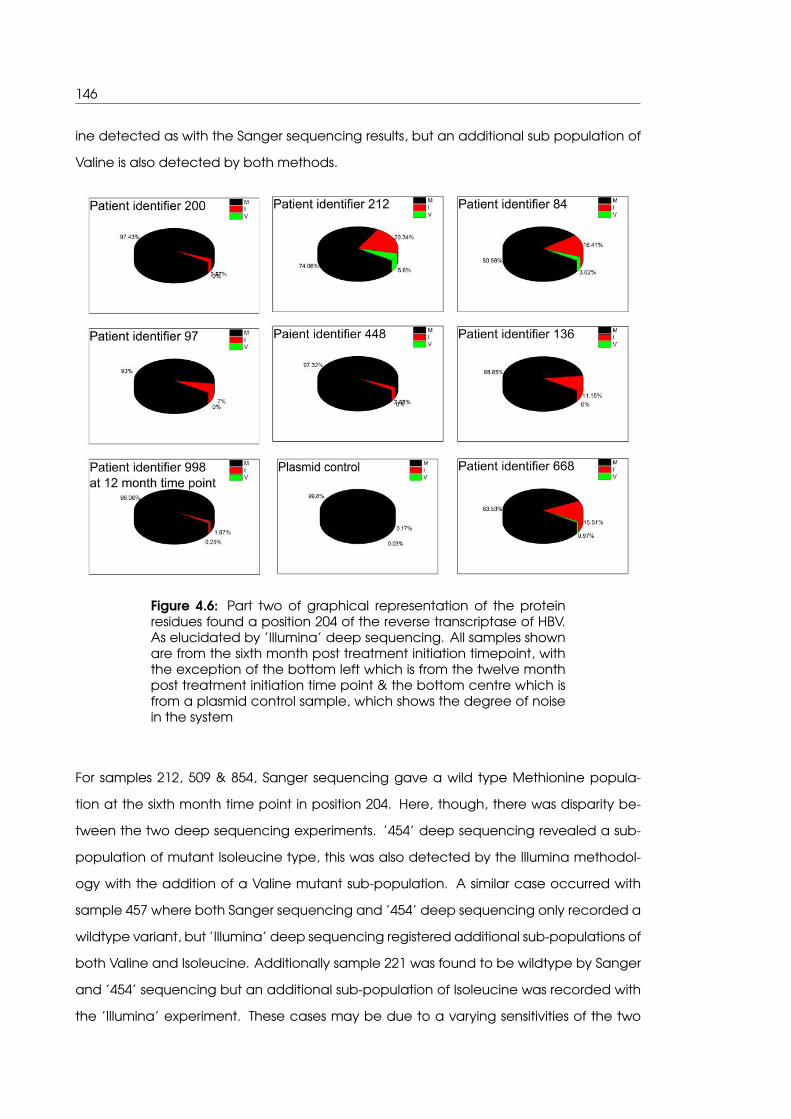
146
ine detected as with the Sanger sequencing results, but an additional sub population of
Valine is also detected by both methods.
Figure 4.6: Part two of graphical representation of the proteinresidues found a position 204 of the reverse transcriptase of HBV.As elucidated by ’Illumina’ deep sequencing. All samples shownare from the sixth month post treatment initiation timepoint, withthe exception of the bottom left which is from the twelve monthpost treatment initiation time point & the bottom centre which isfrom a plasmid control sample, which shows the degree of noisein the system
For samples 212, 509 & 854, Sanger sequencing gave a wild type Methionine popula-
tion at the sixth month time point in position 204. Here, though, there was disparity be-
tween the two deep sequencing experiments. ’454’ deep sequencing revealed a sub-
population of mutant Isoleucine type, this was also detected by the Illumina methodol-
ogy with the addition of a Valine mutant sub-population. A similar case occurred with
sample 457 where both Sanger sequencing and ’454’ deep sequencing only recorded a
wildtype variant, but ’Illumina’ deep sequencing registered additional sub-populations of
both Valine and Isoleucine. Additionally sample 221 was found to be wildtype by Sanger
and ’454’ sequencing but an additional sub-population of Isoleucine was recorded with
the ’Illumina’ experiment. These cases may be due to a varying sensitivities of the two
4. Chapter 4 Results of HBV sequencing 147
deep sequencing protocols.
Sample 136 was initially determined to be Isoleucine only by Sanger sequencing, but
was determined to be a mixture of Methionine and Isoleucine by both deep sequencing
methodologies. it is possible that the Methionine sub-population was masked by a PCR
bias in the Sanger sequencing result
Sample 84 had been determined to be a mixture of wildtype and valine by Sanger se-
quencing. ’Illumina’ added an Isoleucine sub-population, whereas the ’454’ experiment
also detected this Isoleucine population but didn’t see a Valine sub-population.
At this timepoint sample 729 was determined to be a mixture of Methionine and
Isoleucine, this was confirmed by the ’Illumina’ deep sequencing experiment, but was
missed in the earlier ’454’ deep sequencing experiment which recorded only Methion-
ine.
A phylogenetic tree is shown in figure 4.7 here it can be seen that the samples from
the same patient at the same timepoint from either the Sanger sequencing or amplicon
preparation for the Illumina experiment exclusively line up with one another. This was
performed prior to performing the actual Illumina deep sequencing run as a check to
ensure that no sample mix-up had occurred. From this result it is concluded that sample
mix-up is highly unlikely and that the Illumina experiment should proceed.

148
Figure 4.7: A phylogenetic tree comparing sequences from theSanger sequencing and Illumina deep sequencing experiments.Samples from Sanger sequencing begin NH followed by the pa-tient identifier and the timepoint, Samples from the Illumina deepsequencing experiment start ’sam’ followed by the patient iden-tifier and then the timepoint
4.5 Analysis of HBV mutants by Single whole genome se-
quencing
This work was performed at the Department of Virology Royal Free Hospital, London. Use-
ful discussions were had with Dr. Ian Harrison, Dr. Simon Bridge & Dr. John Ambrose.
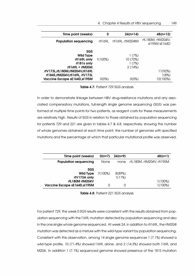
4. Chapter 4 Results of HBV sequencing 149
Time point (weeks) 0 24(n=14) 48(n=12)
Population sequencing rtI169L rtI169L, rtM204IM rtL180M, rtM204IV,sI195M sE164D
SGSWild Type 1 (7%)
rtI169L only 1(100%) 10 (70%)rt181s only 1 (7%)
rtI169L + rtM204I 2 (14%)rtV173L,rtL180M,rtM204V,rtI169L 11(92%)rt184S,rtM204V,rtI169L, rtV173L 1(8%)
Vaccine Escape sE164D,sI195M 0(0%) 0(0%) 12(100%)
Table 4.7: Patient 729 SGS analysis
In order to demonstrate linkage between HBV drug-resistance mutations and any asso-
ciated compensatory mutations, full-length single genome sequencing (SGS) was per-
formed at multiple time points for two patients, as reagent costs for these measurements
are relatively high. Results of SGS in relation to those obtained by population sequencing
for patients 729 and 221 are given in tables 4.7 & 4.8, respectively, showing the number
of whole genomes obtained at each time point, the number of genomes with specified
mutations and the percentage at which that particular mutational profile was observed.
Time point (weeks) 0(n=7) 24(n=9) 48(n=1)
Population sequencing None none rtL180M, rtM204V, rtI195M
SGSWild Type 7(100%) 8(89%)
rtV173A only 1(11%)rtL180M rtM204V 1(100%)
Vaccine Escape sE164D,sI195M 0 0 1(100%)
Table 4.8: Patient 221 SGS analysis
For patient 729, the week 0 SGS results were consistent with the results obtained from pop-
ulation sequencing with the I169L mutation detected by population sequencing and also
in the one single whole genome sequenced. At week 24, in addition to rtI169L, the rtM204I
mutation was detected as a mixture with the wild-type variant by population sequencing.
Consistent with this observation, among 14 single genome sequences 1 (7.1%) showed a
wild-type profile, 10 (71.4%) showed I169L alone, and 2 (14.3%) showed both I169L and
M204. In addition 1 (7.1%) sequenced genome showed presence of the 181S mutation

150
alone. Lamivudine resistance mutation is therefore shown to be present at a level of
14%, theoretically this should be under the detection limit of population type sequenc-
ing, which is normally cited at 20%[Margeridon-Thermet et al., 2009] however this muta-
tion was detected in population sequencing. At week 48 all 12 genomes (100%) show
the same mutational pattern as was observed from population sequencing, therefore
all genomes are drug resistant. At weeks 0 (n=1) and 24 (n=14) none of the sequenced
genomes show mutations in HBsAg; this means they are not capable of vaccine escape.
However, at week 48, all genomes (n=12) show presence of the double vaccine escape
mutant sE164D & sI195M. This implies that at this point all genomes are drug resistant and
capable of vaccine escape. The rt169L mutation in reverse transcriptase is not consid-
ered significant and is therefore considered analogous to wildtype as it is associated with
Adefovir resistance rather than Lamivudine[Ismail et al., 2014, Kim et al., 2013].
For sample 221 the week 0 results are identical to population type sequencing in that all
genomes are of wild type. By week 24 a genome with an accessory rt173 mutation is de-
tected that was not detected in population type sequencing, and at week 48 the results
obtained are similar to population sequencing except that a double vaccine escape
mutant is detected.
As shown in Figure 4.8, phylogentic analysis including the full genome sequences ob-
tained in this study and other full genome sequences of various HBV genotypes obtained
from Genbank, was performed. This analysis confirmed, that the patients studied in this
cohort are infected with HBV genotype A1, as all genomes from the single whole genome
sequencing analysis cluster around the A1 genotype as expected. There was relatively
low genetic distance between genomes obtained in this study generally. Furthermore the
genomes obtained from each patient regardless of time point tend to cluster together.
No evidence was found for recombination. This indicated that the HBV replicating within
this cohort is a typical A1 genotype and suggests that no inter genotype recombination
has occurred. This was performed as different genotypes are known to have different
pathogenicities [Lin and Kao, 2011].
This phylogenetic tree and all others were constructed using the program Fasttree 2, this
program infers approximately-maximum-likelihood phylogenetic trees from nucleotide se-
quences. The default settings of this program were used to draw the trees. The alignment
files, for input into the Fasttree 2 program, were produced from nucleotide sequences us-
ing the program Bioedit. Again the default program settings were used when producing
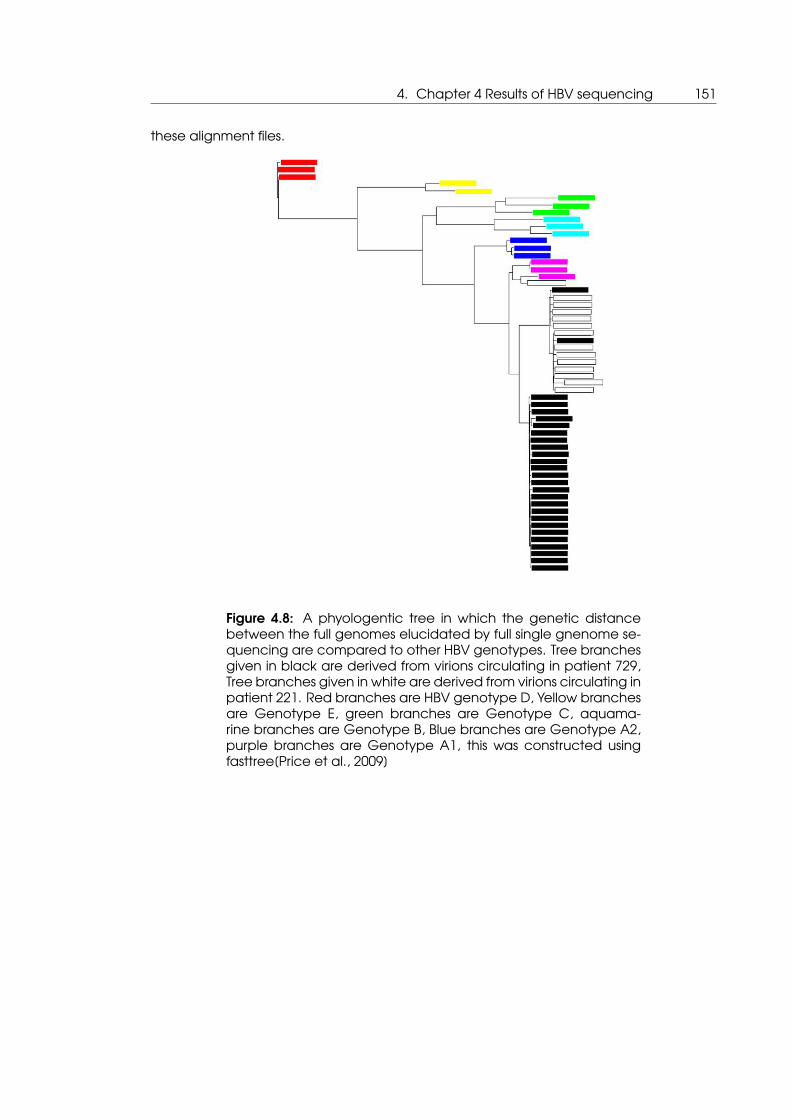
4. Chapter 4 Results of HBV sequencing 151
these alignment files.
Figure 4.8: A phyologentic tree in which the genetic distancebetween the full genomes elucidated by full single gnenome se-quencing are compared to other HBV genotypes. Tree branchesgiven in black are derived from virions circulating in patient 729,Tree branches given in white are derived from virions circulating inpatient 221. Red branches are HBV genotype D, Yellow branchesare Genotype E, green branches are Genotype C, aquama-rine branches are Genotype B, Blue branches are Genotype A2,purple branches are Genotype A1, this was constructed usingfasttree[Price et al., 2009]

152

5. Chapter 5 Results of IRqPCR system measurements 153
5. Chapter 5 Results of IRqPCR system
measurements

154
5.1 Introduction to Results of IRqPCR system measurements
Attempts are made to implement an all optical qPCR system. This system would draw on
experiences on using optical thermometry and heating of a biological sample gained
in making the protein stability measurements. The system would be tested using samples
from the HBV sequencing experiments, such that it was being developed to test a real
life clinical scenario. By using samples from a clinical test case the development of this
system is lent a greater social and commercial impact.
5.2 First IRqPCR system iteration results
The results of the first IRqPCR system design iteration were obtained in part with collabo-
ration from Dr. Sagar Dodderi. Molecular biology work and sample set up was performed
at the Department of Biochemical Engineering, University College London. Operation of
the system was performed at the London Centre for Nanotechnology.
5.2.1 Control qPCR reactions performed in commercial qPCR instrument
to verify qPCR reaction is functional
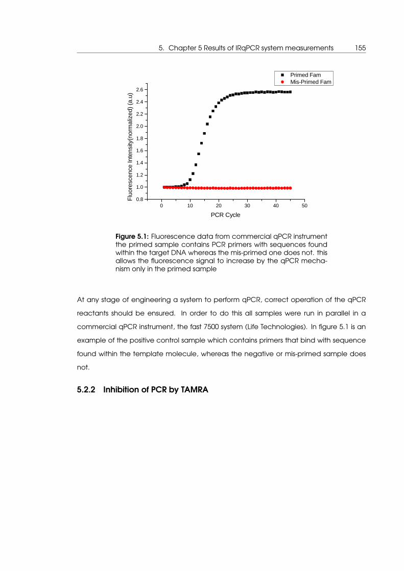
5. Chapter 5 Results of IRqPCR system measurements 155
0 1 0 2 0 3 0 4 0 5 00 . 81 . 01 . 21 . 41 . 61 . 82 . 02 . 22 . 42 . 6
P r i m e d F a m M i s - P r i m e d F a m
Fluore
scenc
e Inte
nsity(
norm
alized
) (a.u)
P C R C y c l e
Figure 5.1: Fluorescence data from commercial qPCR instrumentthe primed sample contains PCR primers with sequences foundwithin the target DNA whereas the mis-primed one does not. thisallows the fluorescence signal to increase by the qPCR mecha-nism only in the primed sample
At any stage of engineering a system to perform qPCR, correct operation of the qPCR
reactants should be ensured. In order to do this all samples were run in parallel in a
commercial qPCR instrument, the fast 7500 system (Life Technologies). In figure 5.1 is an
example of the positive control sample which contains primers that bind with sequence
found within the template molecule, whereas the negative or mis-primed sample does
not.
5.2.2 Inhibition of PCR by TAMRA
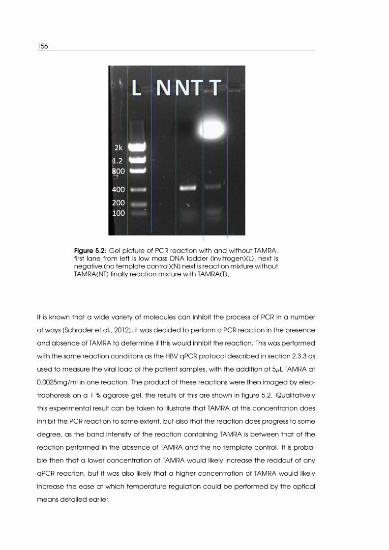
156
Figure 5.2: Gel picture of PCR reaction with and without TAMRA.first lane from left is low mass DNA ladder (invitrogen)(L), next isnegative (no template control)(N) next is reaction mixture withoutTAMRA(NT) finally reaction mixture with TAMRA(T),
It is known that a wide variety of molecules can inhibit the process of PCR in a number
of ways [Schrader et al., 2012], it was decided to perform a PCR reaction in the presence
and absence of TAMRA to determine if this would inhibit the reaction. This was performed
with the same reaction conditions as the HBV qPCR protocol described in section 2.3.3 as
used to measure the viral load of the patient samples, with the addition of 5µL TAMRA at
0.0025mg/ml in one reaction. The product of these reactions were then imaged by elec-
trophoresis on a 1 % agarose gel, the results of this are shown in figure 5.2. Qualitatively
this experimental result can be taken to illustrate that TAMRA at this concentration does
inhibit the PCR reaction to some extent, but also that the reaction does progress to some
degree, as the band intensity of the reaction containing TAMRA is between that of the
reaction performed in the absence of TAMRA and the no template control. It is proba-
ble then that a lower concentration of TAMRA would likely increase the readout of any
qPCR reaction, but it was also likely that a higher concentration of TAMRA would likely
increase the ease at which temperature regulation could be performed by the optical
means detailed earlier.

5. Chapter 5 Results of IRqPCR system measurements 157
5.2.3 Amplification of DNA not detected
qPCR was attempted in the first iteration IRqPCR system in the manner previously de-
scribed in section 2.3.3. The temperature profile to run a two step qPCR program was
ascertained by stepping up through increasing levels of power supply to the infra-red
heating laser, until the power levels that would cause the sample to stabilize at 95 & 60◦C
at the focal point of the infra-red laser, had been established. These power levels were in-
put to the labview control software. This was performed by comparing the fluorescence
of TAMRA of images taken at some infra-red power input, as measured by the micro-
scope.
Prior to initiating the qPCR program an image of FAM fluorescence was taken. This is
shown in figure 5.3. Below this image is an analysis of the fluorescence intensity of FAM
plotted in arbitrary units along the capillary axis. The median and maximum & minimum
values are respectively 1981, 2090 &1723, with a standard deviation of 92. These values
were then compared to values taken subsequent to completing the qPCR program.
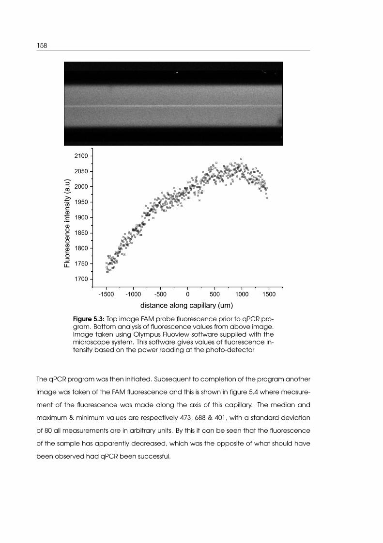
158
-1500 -1000 -500 0 500 1000 1500
1700
1750
1800
1850
1900
1950
2000
2050
2100
Flu
ores
cenc
e in
tens
ity (
a.u)
distance along capillary (um)
Figure 5.3: Top image FAM probe fluorescence prior to qPCR pro-gram. Bottom analysis of fluorescence values from above image.Image taken using Olympus Fluoview software supplied with themicroscope system. This software gives values of fluorescence in-tensity based on the power reading at the photo-detector
The qPCR program was then initiated. Subsequent to completion of the program another
image was taken of the FAM fluorescence and this is shown in figure 5.4 where measure-
ment of the fluorescence was made along the axis of this capillary. The median and
maximum & minimum values are respectively 473, 688 & 401, with a standard deviation
of 80 all measurements are in arbitrary units. By this it can be seen that the fluorescence
of the sample has apparently decreased, which was the opposite of what should have
been observed had qPCR been successful.

5. Chapter 5 Results of IRqPCR system measurements 159
-1500 -1000 -500 0 500 1000 1500 2000
400
450
500
550
600
650
700
Flu
ore
scence
inte
nsi
ty (
a.u
)
distance along capillary (um)
Figure 5.4: Top image FAM probe fluorescence subsequent toqPCR program. Bottom analysis of fluorescence values fromabove image
As it was seen in figure 5.4 that the fluorescence of FAM had a non-homogeneous distri-
bution along the axis of the capillary, it was theorized that potentially molecules of FAM
had moved away from the point of heating due to the Ludwig-Soret effect whereby parti-
cle in a fluid will move down a temperature gradient within that system[Jung et al., 2011].
In that when a temperature gradient exist in a body of solvent such as water, a dissolved
particle will encounter more collisions with the water molecules when at a higher tem-
perature. The resultant effect is that the rate of diffusion of these particles is higher when
being bombarded by collisions with the higher temperature water molecules. This will
cause said particles to move, on average, towards the area of lower water temperature.
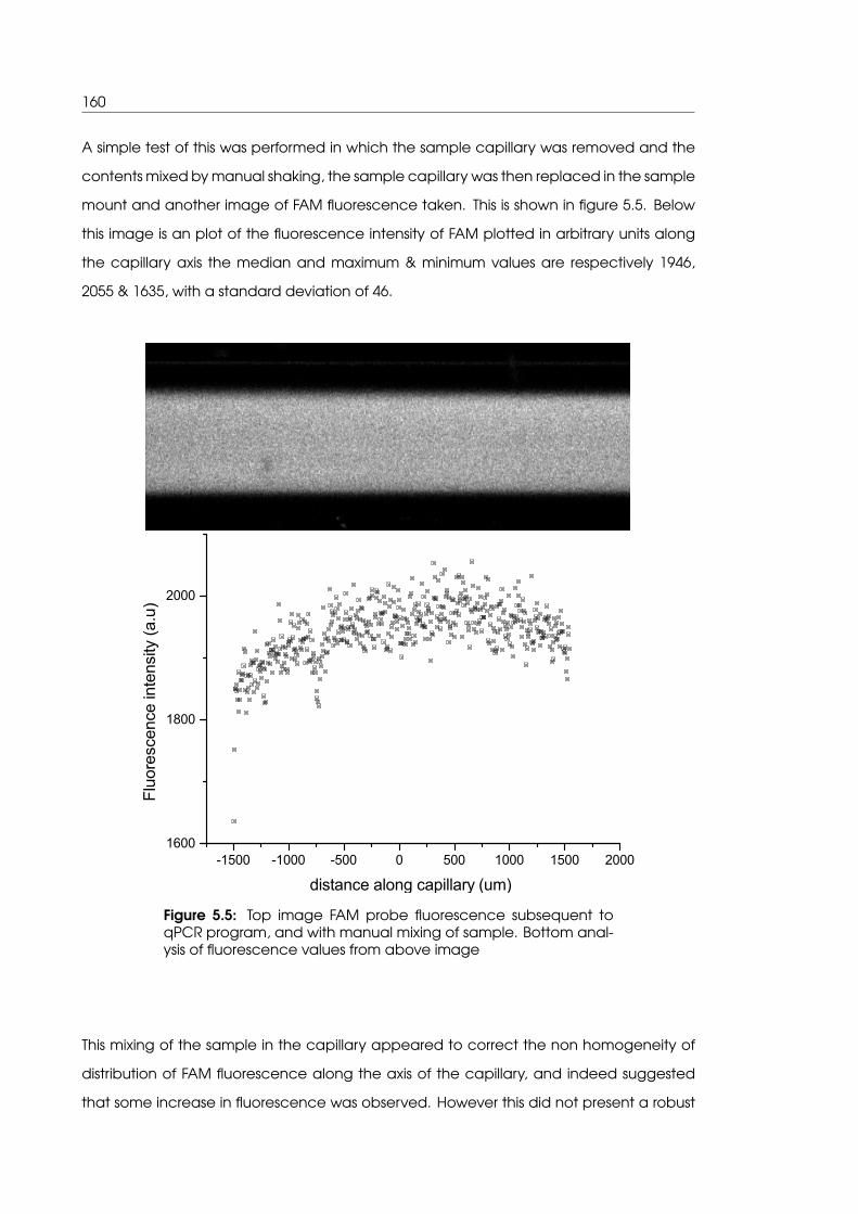
160
A simple test of this was performed in which the sample capillary was removed and the
contents mixed by manual shaking, the sample capillary was then replaced in the sample
mount and another image of FAM fluorescence taken. This is shown in figure 5.5. Below
this image is an plot of the fluorescence intensity of FAM plotted in arbitrary units along
the capillary axis the median and maximum & minimum values are respectively 1946,
2055 & 1635, with a standard deviation of 46.
-1500 -1000 -500 0 500 1000 1500 20001600
1800
2000
Flu
ore
scen
ce in
tens
ity (
a.u)
distance along capillary (um)
Figure 5.5: Top image FAM probe fluorescence subsequent toqPCR program, and with manual mixing of sample. Bottom anal-ysis of fluorescence values from above image
This mixing of the sample in the capillary appeared to correct the non homogeneity of
distribution of FAM fluorescence along the axis of the capillary, and indeed suggested
that some increase in fluorescence was observed. However this did not present a robust
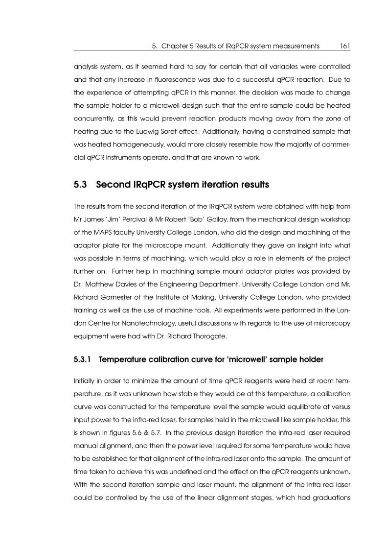
5. Chapter 5 Results of IRqPCR system measurements 161
analysis system, as it seemed hard to say for certain that all variables were controlled
and that any increase in fluorescence was due to a successful qPCR reaction. Due to
the experience of attempting qPCR in this manner, the decision was made to change
the sample holder to a microwell design such that the entire sample could be heated
concurrently, as this would prevent reaction products moving away from the zone of
heating due to the Ludwig-Soret effect. Additionally, having a constrained sample that
was heated homogeneously, would more closely resemble how the majority of commer-
cial qPCR instruments operate, and that are known to work.
5.3 Second IRqPCR system iteration results
The results from the second iteration of the IRqPCR system were obtained with help from
Mr James ’Jim’ Percival & Mr Robert ’Bob’ Gollay, from the mechanical design workshop
of the MAPS faculty University College London, who did the design and machining of the
adaptor plate for the microscope mount. Additionally they gave an insight into what
was possible in terms of machining, which would play a role in elements of the project
further on. Further help in machining sample mount adaptor plates was provided by
Dr. Matthew Davies of the Engineering Department, University College London and Mr.
Richard Gamester of the Institute of Making, University College London, who provided
training as well as the use of machine tools. All experiments were performed in the Lon-
don Centre for Nanotechnology, useful discussions with regards to the use of microscopy
equipment were had with Dr. Richard Thorogate.
5.3.1 Temperature calibration curve for ’microwell’ sample holder
Initially in order to minimize the amount of time qPCR reagents were held at room tem-
perature, as it was unknown how stable they would be at this temperature, a calibration
curve was constructed for the temperature level the sample would equilibrate at versus
input power to the infra-red laser, for samples held in the microwell like sample holder, this
is shown in figures 5.6 & 5.7. In the previous design iteration the infra-red laser required
manual alignment, and then the power level required for some temperature would have
to be established for that alignment of the infra-red laser onto the sample. The amount of
time taken to achieve this was undefined and the effect on the qPCR reagents unknown.
With the second iteration sample and laser mount, the alignment of the infra red laser
could be controlled by the use of the linear alignment stages, which had graduations
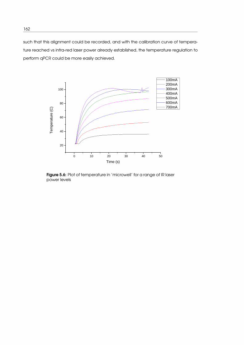
162
such that this alignment could be recorded, and with the calibration curve of tempera-
ture reached vs infra-red laser power already established, the temperature regulation to
perform qPCR could be more easily achieved.
0 1 0 2 0 3 0 4 0 5 0
2 0
4 0
6 0
8 0
1 0 0
Temp
eratur
e (C)
T i m e ( s )
1 0 0 m A 2 0 0 m A 3 0 0 m A 4 0 0 m A 5 0 0 m A 6 0 0 m A 7 0 0 m A
Figure 5.6: Plot of temperature in ’microwell’ for a range of IR laserpower levels

5. Chapter 5 Results of IRqPCR system measurements 163
2 0 0 4 0 03 0
4 0
5 0
6 0
7 0
8 0
9 0
1 0 0
Equili
brium
Temp
eratur
e (C)
P o w e r i n ( m A )
Figure 5.7: Plot of stabilized temperature values in ’microwell’ fora range of IR laser power levels
Despite the enhancement detailed in section 5.3.1, images taken after correctly primed
samples that were shown to have undergone PCR amplification in a commercial qPCR
instrument showed no increase in FAM fluorescence when compared to images taken
before PCR thermocycling in the optical qPCR system using that calibration curve (data
not shown). The decision was therefore made to use a fluorescence microscope as the
imaging platform for the system as live data of TAMRA fluorescence could be fed into
a PID control loop to enable real time temperature regulation which would be entirely
alignment independent and potentially much more tightly regulated.
5.3.2 PID feedback control facilitates tighter temperature regulation
First implementation of PID feedback control was tested and tuned with samples at tem-
peratures lower than required for PCR in order to assess the response of the feedback
loop, without causing the sample to approach the 95 ◦C required for DNA denaturation
as overshoots at this stage were unknown and if the sample boiled it would require reload-
ing the sample holder. The final result of the PID tuning with the system in this configuration
is shown in figure 5.8.
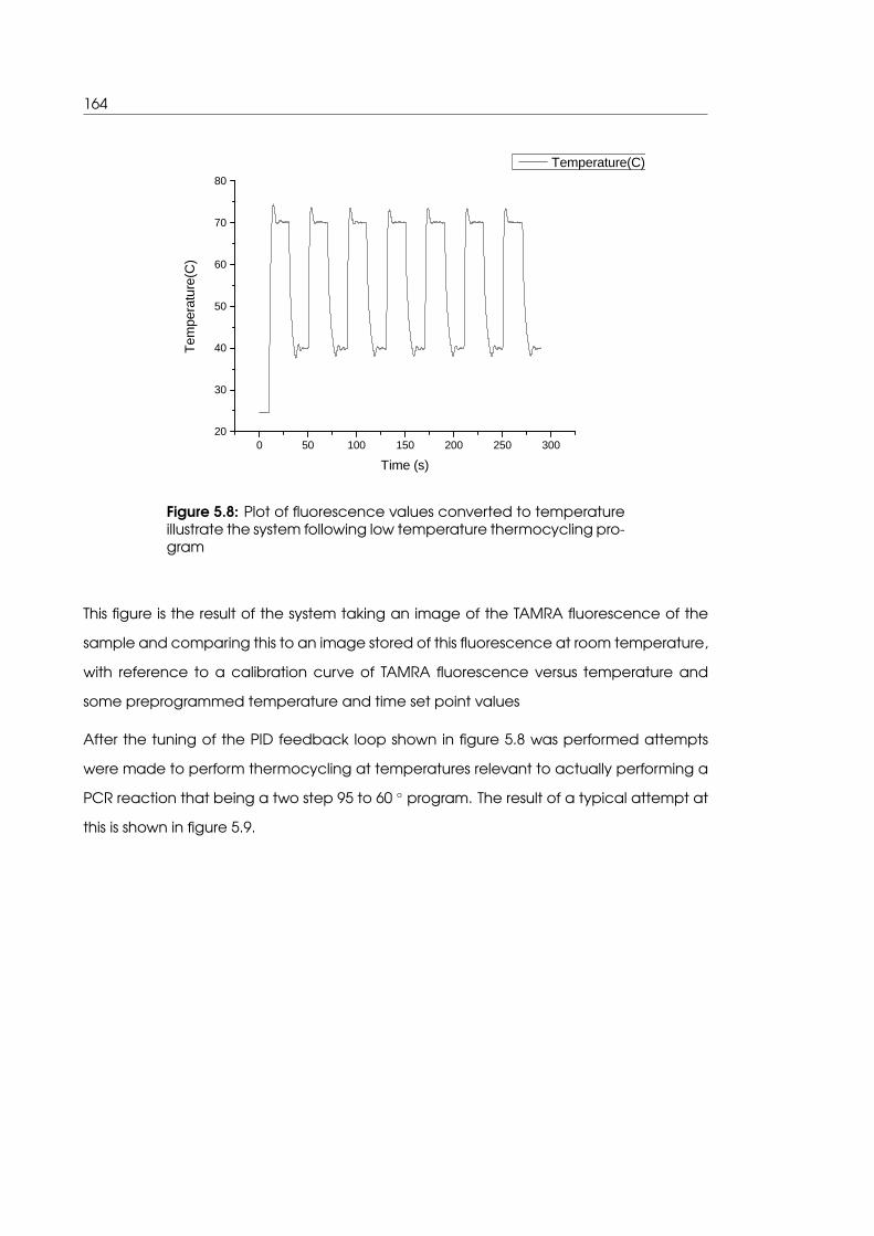
164
0 5 0 1 0 0 1 5 0 2 0 0 2 5 0 3 0 02 0
3 0
4 0
5 0
6 0
7 0
8 0Te
mpera
ture(C
)
T i m e ( s )
T e m p e r a t u r e ( C )
Figure 5.8: Plot of fluorescence values converted to temperatureillustrate the system following low temperature thermocycling pro-gram
This figure is the result of the system taking an image of the TAMRA fluorescence of the
sample and comparing this to an image stored of this fluorescence at room temperature,
with reference to a calibration curve of TAMRA fluorescence versus temperature and
some preprogrammed temperature and time set point values
After the tuning of the PID feedback loop shown in figure 5.8 was performed attempts
were made to perform thermocycling at temperatures relevant to actually performing a
PCR reaction that being a two step 95 to 60 ◦ program. The result of a typical attempt at
this is shown in figure 5.9.
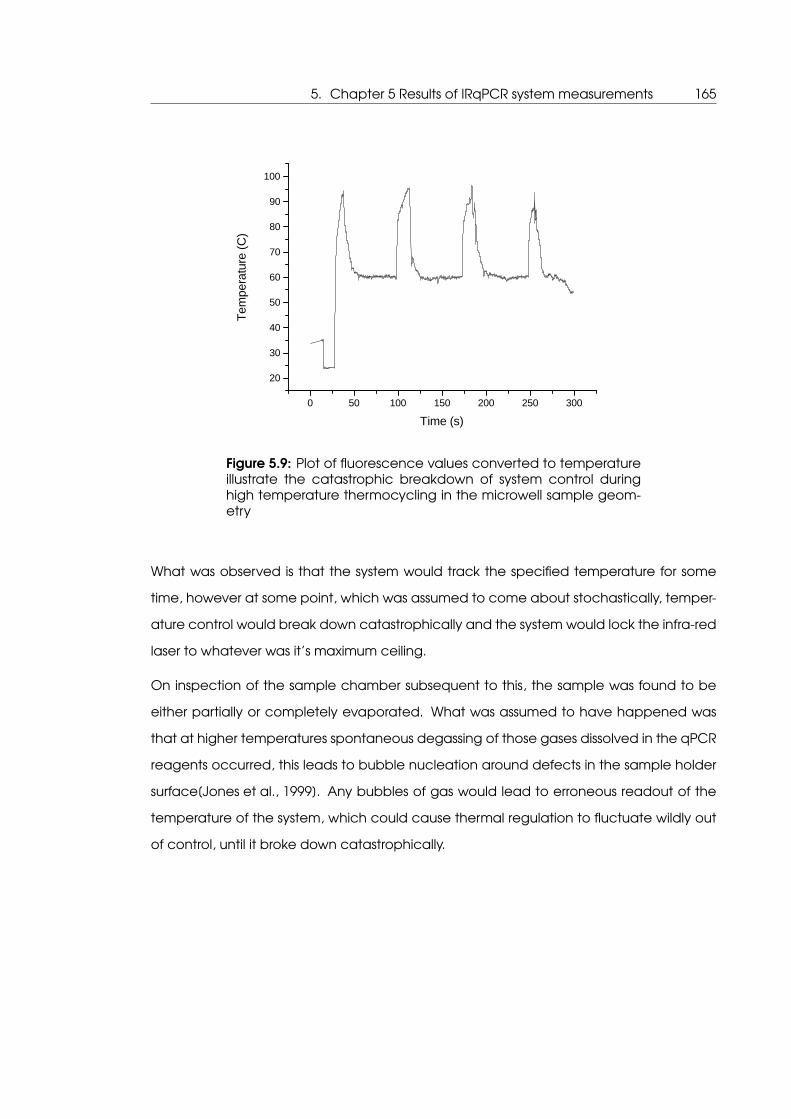
5. Chapter 5 Results of IRqPCR system measurements 165
0 5 0 1 0 0 1 5 0 2 0 0 2 5 0 3 0 02 03 04 05 06 07 08 09 0
1 0 0
Temp
eratur
e (C)
T i m e ( s )
Figure 5.9: Plot of fluorescence values converted to temperatureillustrate the catastrophic breakdown of system control duringhigh temperature thermocycling in the microwell sample geom-etry
What was observed is that the system would track the specified temperature for some
time, however at some point, which was assumed to come about stochastically, temper-
ature control would break down catastrophically and the system would lock the infra-red
laser to whatever was it’s maximum ceiling.
On inspection of the sample chamber subsequent to this, the sample was found to be
either partially or completely evaporated. What was assumed to have happened was
that at higher temperatures spontaneous degassing of those gases dissolved in the qPCR
reagents occurred, this leads to bubble nucleation around defects in the sample holder
surface[Jones et al., 1999]. Any bubbles of gas would lead to erroneous readout of the
temperature of the system, which could cause thermal regulation to fluctuate wildly out
of control, until it broke down catastrophically.

166
Figure 5.10: Light microscopy image of the microwell sampleholder
Light & Scanning electron microscopy was performed of the microwell sample holder to
determine what the condition of the surface was. With light microscopy the surface of the
sample holder appeared to be perfectly smooth as shown in figure 5.10. However Scan-
ning electron microscopy revealed multiple small pores capable of acting as nucleation
sites for bubble formation by spontaneous degassing, this is shown in figure 5.11.

5. Chapter 5 Results of IRqPCR system measurements 167
Figure 5.11: A montage of scanning electron micrographs of themicrowell sample holder taken at different angles and magnifica-tions to assess surface quality of the device
In order to solve the problem of spontaneous degassing occurring and causing bubble
formation leading to catastrophic breakdown of optical thermo-regulation, a number
of changes to the system or protocol were attempted. These changes including flowing
mineral oil into the microwell device prior to loading of the sample, as well as intentionally
degassing the sample in a vacuum bell jar prior to loading into the microwell sample
holder. None of these approaches resulted in a two step PCR program being completed.
Eventually a wider bore capillary was sourced, this was filled with PCR compatible min-
eral oil and the qPCR reagents injected into a central position in the capillary forming a
microbubble of sample surrounded by mineral oil. The objective here being that as the
mineral oil had once completely filled the capillary any small defects that could serve
as nucleation sites for bubble formation by spontaneous degassing would be filled and
therefore excluded. The results of high temperature thermocycling via PID control for this
system setup are shown in figure 5.12.
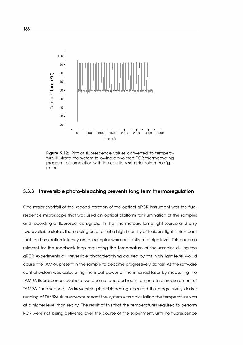
168
-500 0 500 1000 1500 2000 2500 3000 3500
20
30
40
50
60
70
80
90
100
T(C
)
t(s)TimeTime
Figure 5.12: Plot of fluorescence values converted to tempera-ture illustrate the system following a two step PCR thermocyclingprogram to completion with the capillary sample holder configu-ration.
5.3.3 Irreversible photo-bleaching prevents long term thermoregulation
One major shortfall of the second iteration of the optical qPCR instrument was the fluo-
rescence microscope that was used an optical platform for illumination of the samples
and recording of fluorescence signals. In that the mercury lamp light source and only
two available states, those being on or off at a high intensity of incident light. This meant
that the illumination intensity on the samples was constantly at a high level. This became
relevant for the feedback loop regulating the temperature of the samples during the
qPCR experiments as irreversible photobleaching caused by this high light level would
cause the TAMRA present in the sample to become progressively darker. As the software
control system was calculating the input power of the infra-red laser by measuring the
TAMRA fluorescence level relative to some recorded room temperature measurement of
TAMRA fluorescence. As irreversible photobleaching occurred this progressively darker
reading of TAMRA fluorescence meant the system was calculating the temperature was
at a higher level than reality. The result of this that the temperatures required to perform
PCR were not being delivered over the course of the experiment, until no fluorescence
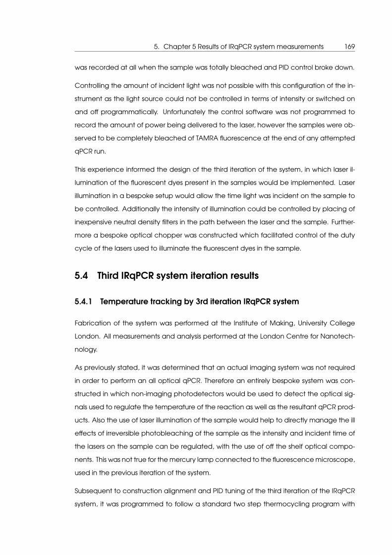
5. Chapter 5 Results of IRqPCR system measurements 169
was recorded at all when the sample was totally bleached and PID control broke down.
Controlling the amount of incident light was not possible with this configuration of the in-
strument as the light source could not be controlled in terms of intensity or switched on
and off programmatically. Unfortunately the control software was not programmed to
record the amount of power being delivered to the laser, however the samples were ob-
served to be completely bleached of TAMRA fluorescence at the end of any attempted
qPCR run.
This experience informed the design of the third iteration of the system, in which laser il-
lumination of the fluorescent dyes present in the samples would be implemented. Laser
illumination in a bespoke setup would allow the time light was incident on the sample to
be controlled. Additionally the intensity of illumination could be controlled by placing of
inexpensive neutral density filters in the path between the laser and the sample. Further-
more a bespoke optical chopper was constructed which facilitated control of the duty
cycle of the lasers used to illuminate the fluorescent dyes in the sample.
5.4 Third IRqPCR system iteration results
5.4.1 Temperature tracking by 3rd iteration IRqPCR system
Fabrication of the system was performed at the Institute of Making, University College
London. All measurements and analysis performed at the London Centre for Nanotech-
nology.
As previously stated, it was determined that an actual imaging system was not required
in order to perform an all optical qPCR. Therefore an entirely bespoke system was con-
structed in which non-imaging photodetectors would be used to detect the optical sig-
nals used to regulate the temperature of the reaction as well as the resultant qPCR prod-
ucts. Also the use of laser illumination of the sample would help to directly manage the ill
effects of irreversible photobleaching of the sample as the intensity and incident time of
the lasers on the sample can be regulated, with the use of off the shelf optical compo-
nents. This was not true for the mercury lamp connected to the fluorescence microscope,
used in the previous iteration of the system.
Subsequent to construction alignment and PID tuning of the third iteration of the IRqPCR
system, it was programmed to follow a standard two step thermocycling program with

170
each section of the cycle being fifteen seconds and one minute at 95 & 60 ◦ C respec-
tively. A plot of the first of these thermocycles can be seen in figure 5.13.
120 140 160 180 200
60
80
100
Tem
pert
ure
(C)
Time (s)
Figure 5.13: Plot of fluorescence values converted to temperaturefor the first cycle to illustrate the system following a two step PCRthermocycling program with the third iteration of the device
With the sample temperature as calculated by the system versus time given. The system
was able to complete 45 such cycles in a program which is shown in figure 5.14 with-
out any apparent loss in control due to the formation of bubbles in the sample or other
artefacts.

5. Chapter 5 Results of IRqPCR system measurements 171
0 500 1000 1500 2000 2500 3000 3500 4000
50
60
70
80
90
100
110
Tem
pert
ure
(C)
Time (s)
Figure 5.14: Plot of fluorescence values converted to tempera-ture illustrate the system following a two step PCR thermocyclingprogram to completion with the third iteration of the device
The third iteration of the IRqPCR system was also able to complete a three step thermo-
cycling program with the first cycle of this shown in figure 5.15 and the full program run
shown in figure 5.16. Both plots are given as the temperature of the sample as calculated
by the system versus time.
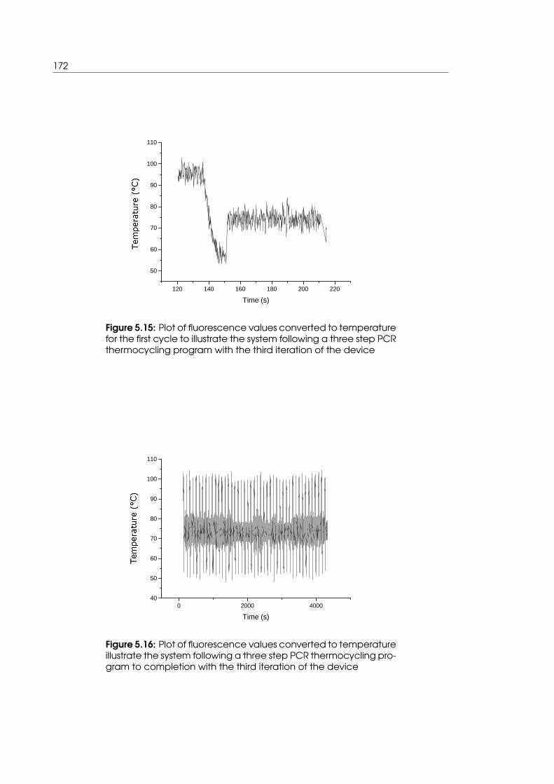
172
120 140 160 180 200 220
50
60
70
80
90
100
110
Tem
pert
ure
(C)
Time (s)
Figure 5.15: Plot of fluorescence values converted to temperaturefor the first cycle to illustrate the system following a three step PCRthermocycling program with the third iteration of the device
0 2000 400040
50
60
70
80
90
100
110
Tem
pert
ure
(C)
Time (s)
Figure 5.16: Plot of fluorescence values converted to temperatureillustrate the system following a three step PCR thermocycling pro-gram to completion with the third iteration of the device
5. Chapter 5 Results of IRqPCR system measurements 173
5.4.2 Irreversible photobleaching does not appreciably affect thermo
regulation or DNA binding dye readout
One major concern with earlier iterations of the IRqPCR system was that TAMRA which was
used to measure and therefore regulate the temperature was susceptible to irreversible
photo-bleaching [Eggeling et al., 1998] was that this would affect temperature regulation
over the course of a thermocycling run, as this could take up to an hour. This problem
presents as the temperature measurements made by the fluorescence of TAMRA are de-
duced relative to some room temperature level of TAMRA fluorescence recorded prior to
the start of the experiment before any heating of the sample occurs. If irreversible pho-
tobleaching occurs at a significant level the fluorescence will be lower than expected
relative to the initial room temeprature measurement of fluorescence. The system seeing
a ’darker’ level of fluorescence will calculate the sample temperature to be higher that
what is actually the case. If a PID control loop is being used, then as the sample becomes
appreciably darker and the system calculates increasingly higher incorrect temperatures
it will accordingly supply less and less power to the infra red heating laser.
A number of measures were designed into the third iteration of the IRqPCR system in or-
der to mitigate this effect. Use of laser illumination as opposed to a filtered wide spectrum
gas lamp light has an inherent advantage in that the spectral range covered 532nm laser
line was far narrower than what would be available using a wide spectrum lamp and
available optical notch filters, this would mean that given the same intensity of incident
light the laser would lay less photons down in the absorption band of TAMRA. Addition-
ally an electronically operated shutter was added to the 532 laser sub system, this would
ensure that light was only hitting the sample when required as the system control soft-
ware would only open the shutter when data was being supplied to the PID. Furthermore
the lockin amplifier allowed extraction of smaller signals of TAMRA intensity from a noisy
background, this means that lower intensity of excitation light could be used to make
measurement of TAMRA fluorescence. Finally the optical chopper had a custom made
blade that reduced the duty cycle of laser to roughly 40% further reducing the amount
of photons hitting the sample and resulting in irreversible photobleaching.
The result of the implementation of these system components can be seen in figure 5.17.
Here the power supplied by the system under PID control to the infra red laser is plotted
against time. It can be seen that there is no significant trend which strongly indicates that

174
irreversible photo bleaching of the sample is not significantly perturbing the ability of the
system to regulate temperature of the sample over the course of an entire thermocycling
program. These data are represented as a ten point rolling average of the data for clarity.
0 5 0 0 1 0 0 0 1 5 0 0 2 0 0 0 2 5 0 0 3 0 0 0 3 5 0 0 4 0 0 0
0
1
2
3
4
5
Powe
r to IR
laser
rolling
avera
ge (A
)
T i m e ( s )
P o w e r t o I R l a s e r r o l l i n g a v e r a g e ( A )
Figure 5.17: Rolling average plot of output values of PID controllerbeing supplied ot IR laser, there is not an increase in this does notdrift up during the course of the hour long thermocycling proce-dure indicating that irreversible bleaching of TAMRA is not affect-ing the temperature regulation of the system
5.4.3 Failure to detect signal resultant from successful PCR in third iteration
IRqPCR system
The third iteration of the qPCR system is able to switch excitation source from the green to
blue laser, in order that the fluorescence from SYBR-Green/FAM would be detected rather
than the fluorescence of TAMRA. This means that a measure of the DNA concentration
present in the sample will be measured instead of measuring the temperature of the sam-
ple. As was the protocol in commercial qPCR instruments the measurement of DNA con-
centration by SYBR-Green/FAM fluorescence was made at the end of each thermocycle
for one second prior to the temperature ramping up again in the denaturation phase
of the thermocycle. During this measurement phase the action of the PID temperature
controller was suspended and a constant value of infra red laser power was supplied. This

5. Chapter 5 Results of IRqPCR system measurements 175
was to ensure approximately homogeneous temperature levels between measurements
of DNA concentration as the fluorescence intensity of SYBR-Green is known to be temper-
ature dependent[Wittwer et al., 1997]. A plot of the fluorescence value of SYBR-Green
taken at the end of each thermocycle is given in figure 5.18. These data were taken dur-
ing a typical two-step thermocycling program as previously described. No increase in
fluorescence attributable to a successful qPCR reaction is observed, moreover an actual
decrease in fluorescence is observed, which may be due to irreversible photo-bleaching
of the sample.
0 2 0 4 0
0 . 1 4
0 . 1 5
0 . 1 6
Detec
tor/ m
onitor
(V)
C y c l e N u m b e r
Figure 5.18: Plot of sybr green fluorescence values recorded atthe end of each thermocycle. The intensity of the illuminationlaser is taken into account by dividing each value with a value ofthe beam monitor taken concurrently

176

6. Chapter 6 Discussion & Conclusions 177
6. Chapter 6 Discussion & Conclusions
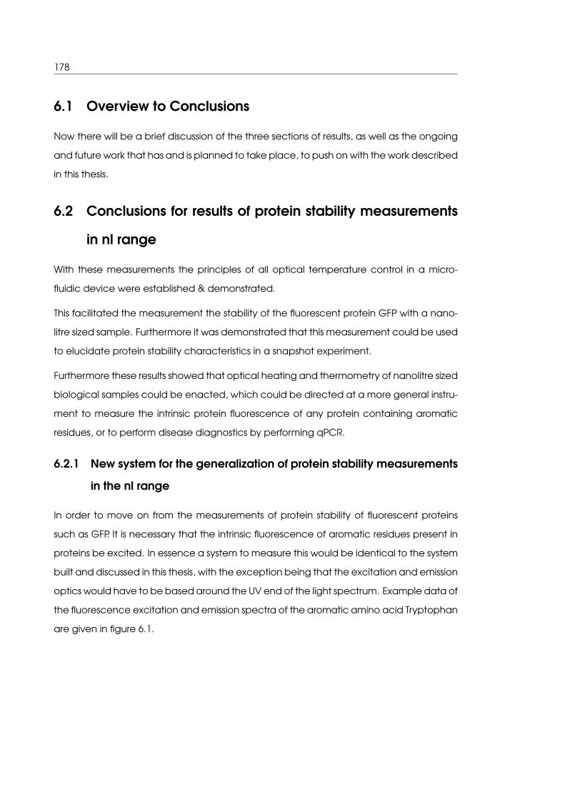
178
6.1 Overview to Conclusions
Now there will be a brief discussion of the three sections of results, as well as the ongoing
and future work that has and is planned to take place, to push on with the work described
in this thesis.
6.2 Conclusions for results of protein stability measurements
in nl range
With these measurements the principles of all optical temperature control in a micro-
fluidic device were established & demonstrated.
This facilitated the measurement the stability of the fluorescent protein GFP with a nano-
litre sized sample. Furthermore it was demonstrated that this measurement could be used
to elucidate protein stability characteristics in a snapshot experiment.
Furthermore these results showed that optical heating and thermometry of nanolitre sized
biological samples could be enacted, which could be directed at a more general instru-
ment to measure the intrinsic protein fluorescence of any protein containing aromatic
residues, or to perform disease diagnostics by performing qPCR.
6.2.1 New system for the generalization of protein stability measurements
in the nl range
In order to move on from the measurements of protein stability of fluorescent proteins
such as GFP. It is necessary that the intrinsic fluorescence of aromatic residues present in
proteins be excited. In essence a system to measure this would be identical to the system
built and discussed in this thesis, with the exception being that the excitation and emission
optics would have to be based around the UV end of the light spectrum. Example data of
the fluorescence excitation and emission spectra of the aromatic amino acid Tryptophan
are given in figure 6.1.
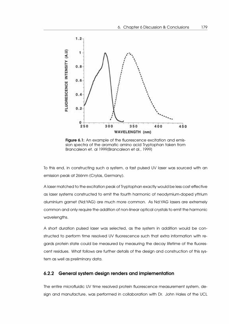
6. Chapter 6 Discussion & Conclusions 179
Figure 6.1: An example of the fluorescence excitation and emis-sion spectra of the aromatic amino acid Tryptophan taken fromBrancaleon et. al 1999[Brancaleon et al., 1999]
To this end, in constructing such a system, a fast pulsed UV laser was sourced with an
emission peak at 266nm (Crylas, Germany).
A laser matched to the excitation peak of Tryptophan exactly would be less cost effective
as laser systems constructed to emit the fourth harmonic of neodymium-doped yttrium
aluminium garnet (Nd:YAG) are much more common. As Nd:YAG lasers are extremely
common and only require the addition of non-linear optical crystals to emit the harmonic
wavelengths.
A short duration pulsed laser was selected, as the system in addition would be con-
structed to perform time resolved UV fluorescence such that extra information with re-
gards protein state could be measured by measuring the decay lifetime of the fluores-
cent residues. What follows are further details of the design and construction of this sys-
tem as well as preliminary data.
6.2.2 General system design renders and implementation
The entire microfluidic UV time resolved protein fluorescence measurement system, de-
sign and manufacture, was performed in collaboration with Dr. John Hales of the UCL
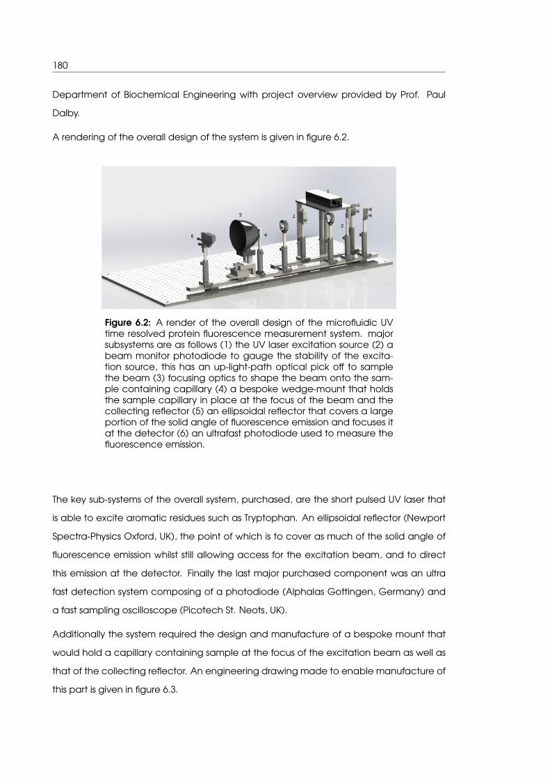
180
Department of Biochemical Engineering with project overview provided by Prof. Paul
Dalby.
A rendering of the overall design of the system is given in figure 6.2.
Figure 6.2: A render of the overall design of the microfluidic UVtime resolved protein fluorescence measurement system. majorsubsystems are as follows (1) the UV laser excitation source (2) abeam monitor photodiode to gauge the stability of the excita-tion source, this has an up-light-path optical pick off to samplethe beam (3) focusing optics to shape the beam onto the sam-ple containing capillary (4) a bespoke wedge-mount that holdsthe sample capillary in place at the focus of the beam and thecollecting reflector (5) an ellipsoidal reflector that covers a largeportion of the solid angle of fluorescence emission and focuses itat the detector (6) an ultrafast photodiode used to measure thefluorescence emission.
The key sub-systems of the overall system, purchased, are the short pulsed UV laser that
is able to excite aromatic residues such as Tryptophan. An ellipsoidal reflector (Newport
Spectra-Physics Oxford, UK), the point of which is to cover as much of the solid angle of
fluorescence emission whilst still allowing access for the excitation beam, and to direct
this emission at the detector. Finally the last major purchased component was an ultra
fast detection system composing of a photodiode (Alphalas Gottingen, Germany) and
a fast sampling oscilloscope (Picotech St. Neots, UK).
Additionally the system required the design and manufacture of a bespoke mount that
would hold a capillary containing sample at the focus of the excitation beam as well as
that of the collecting reflector. An engineering drawing made to enable manufacture of
this part is given in figure 6.3.
6. Chapter 6 Discussion & Conclusions 181
Figure 6.3: An engineering drawing of the ’wedge’ mount used toconstrain the sample in the microfluidic UV time resolved proteinfluorescence measurement system
The part was designed in Solidworks (Dassault systemes Vélizy-Villacoublay, France) and
was sent for automated computer aided manufacturing and machining by Protolabs
(Maple Plain, USA) With some re-machining and finishing work performed at the Institute
of Making, University College London.
A photo of the wedge mount subsequent to manufacturing & finishing with the sample
capillary mounted in place is shown in figure 6.4.

182
Figure 6.4: Wedge mount with sample capillary mounted
A rendering of the system design with the wedge mount inserted into the collecting re-
flector in the main light path is shown in figure 6.5.
Figure 6.5: Render of wedge mount with sample capillarymounted in light path
A picture of this subsystem aligned is given in figure 6.6. a beam block is placed directly in
the light path between the sample and the detector to block any excitation light passing
straight through the capillary and sample from hitting the detector directly, as this would
overwhelm the fluorescence signal.
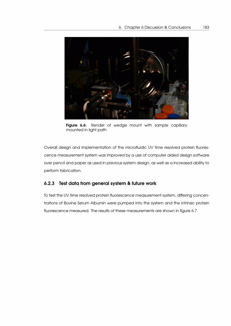
6. Chapter 6 Discussion & Conclusions 183
Figure 6.6: Render of wedge mount with sample capillarymounted in light path
Overall design and implementation of the microfluidic UV time resolved protein fluores-
cence measurement system was improved by a use of computer aided design software
over pencil and paper as used in previous system design, as well as a increased ability to
perform fabrication.
6.2.3 Test data from general system & future work
To test the UV time resolved protein fluorescence measurement system, differing concen-
trations of Bovine Serum Albumin were pumped into the system and the intrinsic protein
fluorescence measured. The results of these measurements are shown in figure 6.7.
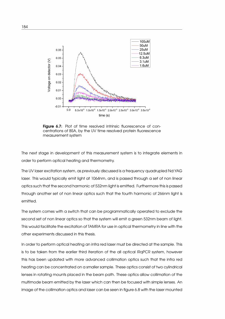
184
Figure 6.7: Plot of time resolved intrinsic fluorescence of con-centrations of BSA, by the UV time resolved protein fluorescencemeasurement system
The next stage in development of this measurement system is to integrate elements in
order to perform optical heating and thermometry.
The UV laser excitation system, as previously discussed is a frequency quadrupled Nd:YAG
laser. This would typically emit light at 1064nm, and is passed through a set of non linear
optics such that the second harmonic of 532nm light is emitted. Furthermore this is passed
through another set of non linear optics such that the fourth harmonic of 266nm light is
emitted.
The system comes with a switch that can be programmatically operated to exclude the
second set of non linear optics so that the system will emit a green 532nm beam of light.
This would facilitate the excitation of TAMRA for use in optical thermometry in line with the
other experiments discussed in this thesis.
In order to perform optical heating an infra red laser must be directed at the sample. This
is to be taken from the earlier third iteration of the all optical IRqPCR system, however
this has been updated with more advanced collimation optics such that the infra red
heating can be concentrated on a smaller sample. These optics consist of two cylindrical
lenses in rotating mounts placed in the beam path. These optics allow collimation of the
multimode beam emitted by the laser which can then be focused with simple lenses. An
image of the collimation optics and laser can be seen in figure 6.8 with the laser mounted

6. Chapter 6 Discussion & Conclusions 185
in the background and the two rotating cylindrical lens mounts in the foreground.
Figure 6.8: Infra red laser with new collimation optics (1) is theinfra red laser (2) are the two rotating lens mounts with cylindricallenses
Additionally in order to align the infra red beam with the sample it was decided to utilize
a dichroic mirror that is reflective to UV light but transmits infra red light. For this purpose a
2 inch 266nm laser line mirror from Melles Griot is placed in the line of the intended beam
path of the infra red laser. The position of this combining optic is shown in a render of the
system from a top down view in figure 6.9 the path of the UV laser beam is shown in blue,
the infra red beam is shown in red and the combining optic is indicated by a label.
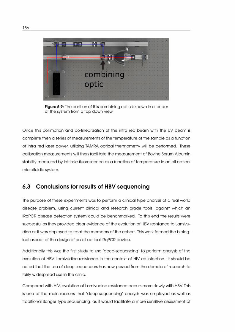
186
Figure 6.9: The position of this combining optic is shown in a renderof the system from a top down view
Once this collimation and co-linearization of the infra red beam with the UV beam is
complete then a series of measurements of the temperature of the sample as a function
of infra red laser power, utilizing TAMRA optical thermometry will be performed. These
calibration measurements will then facilitate the measurement of Bovine Serum Albumin
stability measured by intrinsic fluorescence as a function of temperature in an all optical
microfluidic system.
6.3 Conclusions for results of HBV sequencing
The purpose of these experiments was to perform a clinical type analysis of a real world
disease problem, using current clinical and research grade tools, against which an
IRqPCR disease detection system could be benchmarked. To this end the results were
successful as they provided clear evidence of the evolution of HBV resistance to Lamivu-
dine as it was deployed to treat the members of the cohort. This work formed the biolog-
ical aspect of the design of an all optical IRqPCR device.
Additionally this was the first study to use ’deep-sequencing’ to perform analysis of the
evolution of HBV Lamivudine resistance in the context of HIV co-infection. It should be
noted that the use of deep sequencers has now passed from the domain of research to
fairly widespread use in the clinic.
Compared with HIV, evolution of Lamivudine resistance occurs more slowly with HBV. This
is one of the main reasons that ‘deep sequencing’ analysis was employed as well as
traditional Sanger type sequencing, as it would facilitate a more sensitive assessment of

6. Chapter 6 Discussion & Conclusions 187
Lamivudine resistance mutations.
This improved detection sensitivity of deep sequencing has been previously reported ver-
sus traditional Sanger type sequencing. However some criticisms are that deep sequenc-
ing is prone to false positive results for rare mutant detection, in that these are read errors
based on poor understanding of these new sequencing technologies. To address this a
sensitivity of mutant detection was set at 1% and a very high read quality cut off score
was imposed.
No mutation between Methionine and Isoleucine at position 204 was found at initiation
of treatment with Lamivudine, by deep sequencing, as was to be expected. At the sixth
month time point the amount of this mutation was higher in patients that also showed
this mutation by traditional Sanger type sequencing. All patients that had shown muta-
tion from Methionine to Isoleucine by deep sequencing at sixth months, then went on
to show mutation from Isoleucine to Valine at position 204 by twelve month by Sanger
sequencing. This is consistent with the commonly held observation of lamivudine HBV re-
sistance progressing from the wild type Methionine at position 204 through Isoleucine to
Valine.
These results were corroborated using other techniques such as single genome whole
sequencing which lends veracity that the results are not technical artefacts of using novel
(deep sequencing) technology to perform these analyses.
6.4 Conclusions for results of IRqPCR system measurements
As was shown in the results for the third iteration of an all optical IRqPCR system. The sys-
tem was shown to be able to move quickly and precisely through all the thermal condi-
tions required in a commercial instrument to perform qPCR reactions of HBV polymerase.
Additionally it was shown that by the use of measures such as optical chopping of any
incident light and by using a shutter to further reduce this, that bleaching of the sample
was not affecting the temperature regulation.
Despite of this it was shown that the fluorescence intensity of the DNA binding reporter
dye did not increase in a manner that would indicate that the amount of DNA PCR prod-
uct was increasing exponentially as occurs in a functioning PCR reaction. A brief dis-
cussion on the most likely cause of failure will now occur, as well as a discussion of what
is being implemented in the next iteration of the system in order to build an all optical
188
IRqPCR system.
6.4.1 Possible reasons for failure of qPCR reaction
The capillary sample holder was selected as it had a sufficient enough internal bore such
that the capillary could be filled with PCR compatible mineral oil and then a bubble of
qPCR mix injected into the centre. The ends of the capillary were then sealed by the use
of molten sealing wax and the sample bubble aligned into the beam path by moving
the capillary up and down manually in it’s mounting clips. This was performed as the
mineral oil covering on the inside of the capillary was theorized and illustrated by earlier
experiments to prevent bubble formation, which crippled the optical thermo-regulation
in earlier iterations of the system.
However this may have included a critical failure into the design of the system. As the
Beer-Lambert law states that the intensity of light transmitted in a material decreases
exponentially as a function of length travelled through that material. Given by:
I = I0 exp−µx (6.1)
Where I is the current intensity of light as a proportion of the initial light intensity.
I0 is the initial light intensity µ a linear attenuation coefficient that is related to the
wavelength of light, this coefficient value was taken from the experiments of Hale &
Querry[Hale and Querry, 1973] & x is the distance passed through the material.
A plot of the transmission of light at 1460nm, which is the wavelength of the infra red
heating laser. As a percentage of total available light, as a function of distance travelled
through water contained in the 700 µM internal diameter of the capillary, is given in figure
6.10.
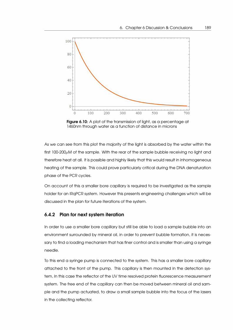
6. Chapter 6 Discussion & Conclusions 189
Figure 6.10: A plot of the transmission of light, as a percentage at1460nm through water as a function of distance in microns
As we can see from this plot the majority of the light is absorbed by the water within the
first 100-200µM of the sample. With the rear of the sample bubble receiving no light and
therefore heat at all. It is possible and highly likely that this would result in inhomogeneous
heating of the sample. This could prove particularly critical during the DNA denaturation
phase of the PCR cycles.
On account of this a smaller bore capillary is required to be investigated as the sample
holder for an IRqPCR system. However this presents engineering challenges which will be
discussed in the plan for future iterations of the system.
6.4.2 Plan for next system iteration
In order to use a smaller bore capillary but still be able to load a sample bubble into an
environment surrounded by mineral oil, in order to prevent bubble formation, it is neces-
sary to find a loading mechanism that has finer control and is smaller than using a syringe
needle.
To this end a syringe pump is connected to the system. This has a smaller bore capillary
attached to the front of the pump. This capillary is then mounted in the detection sys-
tem, In this case the reflector of the UV time resolved protein fluorescence measurement
system. The free end of the capillary can then be moved between mineral oil and sam-
ple and the pump actuated, to draw a small sample bubble into the focus of the lasers
in the collecting reflector.
190
A control program for the syringe pump has been written in Labview that allows specific
volumes of liquid to be drawn and differing flow rates and directions to be assigned to
the pump. Additionally the sample can be jittered back and forth in front of the infra red
beam focus to further facilitate homogeneous heating of the sample bubble.
As this design iteration of the IRqPCR system is being integrated with the UV time resolved
protein fluorescence measurement system, there are certain physical constraints that do
not facilitate the addition of a blue laser to excite the DNA binding dye. However the
DNA binding dye SYBR-green can be replaced by Ethidium Bromide which is able to be
excited by the UV laser and also can be used as a reporter of DNA concentration in
qPCR, although it does have a lower boost in quantum yield on DNA binding compared
to SYBR-green.
The optical thermometry can be performed by placing the UV laser into the 532nm green
emission mode where it can be used to excite TAMRA. However development of a com-
plex Labview control software program must be performed before these experiments are
attempted.

7. Chapter 7 Commercialization 191
7. Chapter 7 Commercialization
192
7.1 Overview to commercialization
The work presented in this thesis was performed largely from a viewpoint of attempting to
engineer systems that can perform useful measurements of biological entities, in such a
manner that there is some advantage over pre-existing technologies.
With this in mind it could be said that the thesis is more concerned with the engineering of
useful technology rather than of measuring some aspect of nature more accurately than
previously performed. So with this in mind an exploration of how the work presented in
this thesis sits within a commercial setting will be undertaken, as it would be fairly obvious
that a newly developed technology cannot exist in an economic vacuum.
7.1.1 Commercial target space exploration
There are two main applications for the technology presented in this thesis. These being,
firstly measurements of protein stability by the measurement of fluorescence as a func-
tion of induced changes in the temperature of the protein. Secondly the detection of
disease by the use of qPCR where fluorescence is detected of DNA binding dyes after
amplification of specific DNA sequences by the polymerase chain reaction.
So the commercial target spaces, that the technology presented in this thesis aims to
compete in, are the manufacture and sale of microplate readers an example of which is
shown in figure 7.1 and other associated detection systems used for the measurement of
protein fluorescence to gauge protein stability.
As well ’qPCR machines’ which are usually composed of a temperature controlled heat-
ing block attached to a fluorimeter. An exploration of these two main target spaces will
be performed individually later on in this chapter.

7. Chapter 7 Commercialization 193
Figure 7.1: An example of a "microplate reader" instrument , thatthis work would seek to subvert
7.1.2 IP appraisal
The work in this thesis was performed with commercialization in mind. From conception in-
tellectual property was secured in the form of patent PCT/GB2010051001 held by former
post doctoral research associate Matthieu Gaudet together with Profs. Gabriel Aeppli
and Paul Dalby who are providing supervision to the project. The patent covers the de-
velopment of a system that uses pure optics to miniaturize fluorimetry measurements and
perform qPCR such that ultra-rapid measurement and high throughput can be achieved.
7.1.3 Industrial partners & collaboration
With significant funding from BBSRC BRIC (Biotechnology Research Industry Club), the
work presented in this thesis has been designed from the ground up with a view towards
the industrial sector and commercialization. BRIC was established to provide a mecha-
nism by which the UK scientific research councils and UK bio-processing industry could
collaborate to provide new solutions to problems facing that sector. As the work pre-
sented in this thesis was funded largely through this mechanism it is natural that there is a
heavy bias towards commercialization and real product development.
To this end, patent protection has already been sought in association with UCL Business
(UCLB), whose mission is to help support and commercialize research from UCL. There
194
is an ongoing collaboration and periodic interaction between their business manager,
assigned to our project, and our research group.
Additionally the work has benefited from interactions with Bio Nano Consulting (BNC) who
have arranged exposure with key industry partners, for example GlaxoSmithKline plc who
were shown the results at a meeting at their facility in Stevenage.
7.2 Commercialization of protein fluorescence measure-
ment
The first commercial product space that the work in this thesis can be targeted at is in the
measurement of protein fluorescence in an industrial and research setting.
7.2.1 Micro-plate readers/ fluorescence spectrometers as a commercial
target
Micro-plate readers and fluorescence spectrometers are a common instrument in both
research and industrial biological/biochemical analysis.
Typically they are composed of:
an illumination source which can be used to excite fluorophores, this could be a series of
lasers, LEDs or a wide spectrum lamp with a collection of interchangeable filters.
A sample holder, typically this will be a large cuvette, an example of which is given in
figure7.2 or a micro-plate. Here the micro-plate is an array of many smaller cuvettes
with the number of elements in the array ranging from 6 to 3000, an example of this is
given in figure7.3. The shift from using fluorescence cuvettes to micro-plates displays that
the industry reacted to the need to parallelize the measurements made by fluorescence
spectrometers. The sample holder in the case of a micro-plate reader will have a actu-
ated stage that can shift either the illumination source and detector between wells, or
move the plate around such that the well presented to the detector and source can be
varied.
The final component of any such system is a detector, which may have a range of
changeable optical filters in front of it. A great many micro-plate readers and fluores-
cence spectrometers will also have a form of temperature control such as a water bath
or dry heating block connected to the sample holder such that measurements made by

7. Chapter 7 Commercialization 195
the system can be performed as a function of temperature.
Figure 7.2: An example of a cuvette used to hold a sample intraditional fluorescence measurements of biological samples.
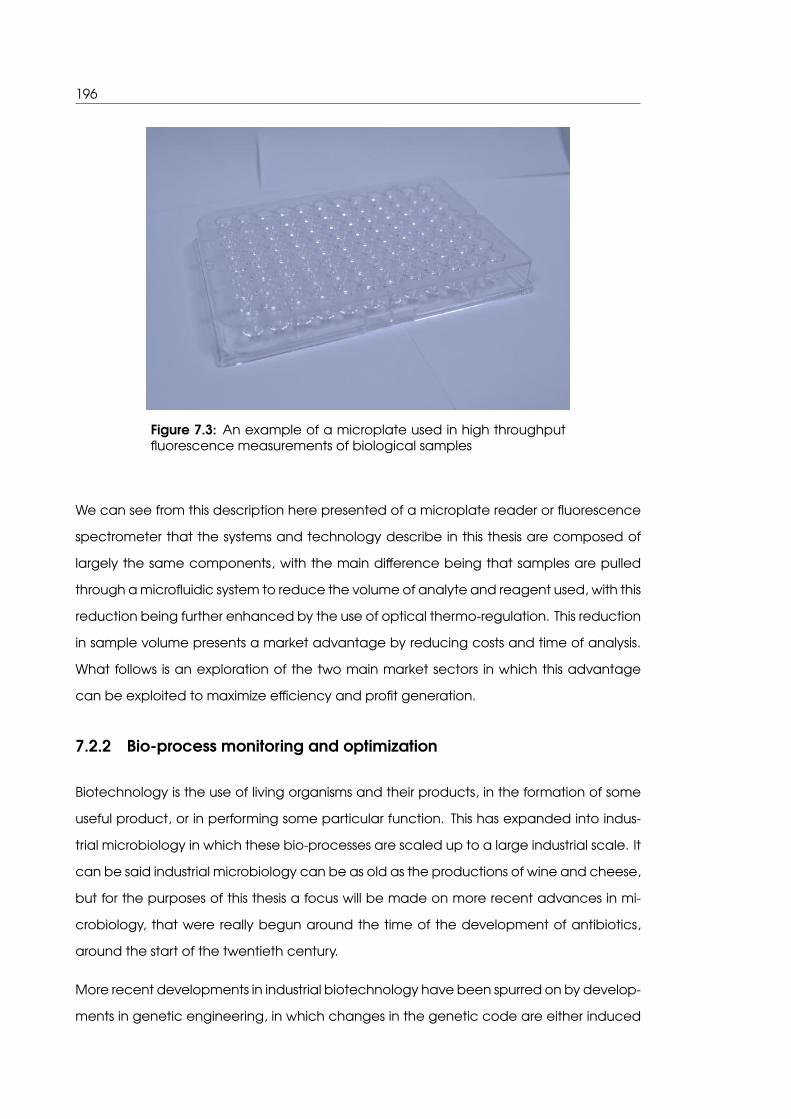
196
Figure 7.3: An example of a microplate used in high throughputfluorescence measurements of biological samples
We can see from this description here presented of a microplate reader or fluorescence
spectrometer that the systems and technology describe in this thesis are composed of
largely the same components, with the main difference being that samples are pulled
through a microfluidic system to reduce the volume of analyte and reagent used, with this
reduction being further enhanced by the use of optical thermo-regulation. This reduction
in sample volume presents a market advantage by reducing costs and time of analysis.
What follows is an exploration of the two main market sectors in which this advantage
can be exploited to maximize efficiency and profit generation.
7.2.2 Bio-process monitoring and optimization
Biotechnology is the use of living organisms and their products, in the formation of some
useful product, or in performing some particular function. This has expanded into indus-
trial microbiology in which these bio-processes are scaled up to a large industrial scale. It
can be said industrial microbiology can be as old as the productions of wine and cheese,
but for the purposes of this thesis a focus will be made on more recent advances in mi-
crobiology, that were really begun around the time of the development of antibiotics,
around the start of the twentieth century.
More recent developments in industrial biotechnology have been spurred on by develop-
ments in genetic engineering, in which changes in the genetic code are either induced

7. Chapter 7 Commercialization 197
in an organism by site directed mutagenesis, or randomly walked in by error prone PCR in
a process known as directed evolution, in an attempt to improve that organism’s ability
to perform some useful function.
During this process of optimizing the performance of an organism or bio-product, it is nec-
essary that measurement be made of the stability of said organism or product. This is an
opportunity in which it is highly likely that a measurement of protein stability as a function
of temperature will be made, by the use of a micro plate reader or fluorescence spec-
trometer. The total industrial biotechnology sector in which these measurements are key
is valued at several billion dollars (US). On account of this there are a great many man-
ufactures of measurement equipment who produce Fluorescence spectrometers and
micro-plate readers, including but not limited to: Eppendorf, Perkin Elmer, Bruker, BMG
Labtech, Berthold, Biotek, Thermo Fisher & Roche.
It has been shown that the technology outlined in this thesis has the ability to perform
these types of measurements with a far smaller sample volume, the aim in commercial-
ization would be therefore to exploit the technology described in the patent to gain li-
censing dues from one of the major players already operating to manufacture this class
of instrumentation.
Ongoing efforts to generalize the measurements of protein fluorescence as a function of
temperature by measuring intrinsic protein fluorescence have already been enacted to
further this aim. The main barrier to entry for deploying this technology for commercial
gain, is that a substantial amount of work is still required to develop the technology into
a bench-top instrument, suitable for use by non-specialist engineering personnel. This
would include a large amount of industrial design work, and programming, to make the
device "process-scientist" proof. It might be hoped that if the technology was licensed to
a larger organization, that this risk could be passed on to them.
7.2.3 Drug discovery pipeline operation
Fluorescence spectrometers and micro-plate readers are also heavily used in the drug
development work of pharmaceutical firms. Here the interaction of small molecule in-
hibitors with protein targets known to be implicated in disease needs to be tested in
terms of binding strength. As the binding strength of a small molecule inhibitor correlates
strongly with its ability to cause inhibition of some disease causing protein. This can be
measured in a system such as ours as the rate of thermal denaturation of a protein will
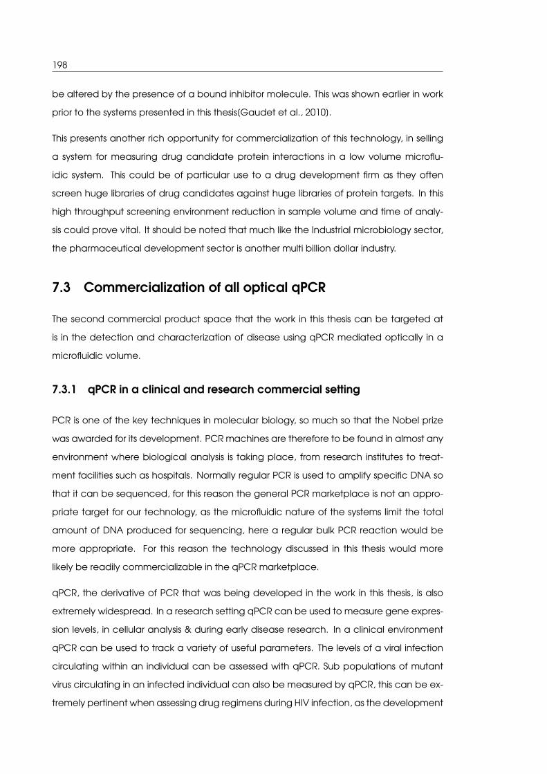
198
be altered by the presence of a bound inhibitor molecule. This was shown earlier in work
prior to the systems presented in this thesis[Gaudet et al., 2010].
This presents another rich opportunity for commercialization of this technology, in selling
a system for measuring drug candidate protein interactions in a low volume microflu-
idic system. This could be of particular use to a drug development firm as they often
screen huge libraries of drug candidates against huge libraries of protein targets. In this
high throughput screening environment reduction in sample volume and time of analy-
sis could prove vital. It should be noted that much like the Industrial microbiology sector,
the pharmaceutical development sector is another multi billion dollar industry.
7.3 Commercialization of all optical qPCR
The second commercial product space that the work in this thesis can be targeted at
is in the detection and characterization of disease using qPCR mediated optically in a
microfluidic volume.
7.3.1 qPCR in a clinical and research commercial setting
PCR is one of the key techniques in molecular biology, so much so that the Nobel prize
was awarded for its development. PCR machines are therefore to be found in almost any
environment where biological analysis is taking place, from research institutes to treat-
ment facilities such as hospitals. Normally regular PCR is used to amplify specific DNA so
that it can be sequenced, for this reason the general PCR marketplace is not an appro-
priate target for our technology, as the microfluidic nature of the systems limit the total
amount of DNA produced for sequencing, here a regular bulk PCR reaction would be
more appropriate. For this reason the technology discussed in this thesis would more
likely be readily commercializable in the qPCR marketplace.
qPCR, the derivative of PCR that was being developed in the work in this thesis, is also
extremely widespread. In a research setting qPCR can be used to measure gene expres-
sion levels, in cellular analysis & during early disease research. In a clinical environment
qPCR can be used to track a variety of useful parameters. The levels of a viral infection
circulating within an individual can be assessed with qPCR. Sub populations of mutant
virus circulating in an infected individual can also be measured by qPCR, this can be ex-
tremely pertinent when assessing drug regimens during HIV infection, as the development

7. Chapter 7 Commercialization 199
of resistance to one drug may precipitate the use of another.
Because of the widespread use of qPCR machines they are manufactured by a large
number of organizations, including but not limited to: Agilent, Beckton Dickinson, Life
Technologies, Bio-rad & Thermo Fisher. The current sales volume of qPCR instrumentation
is thought to be in excess of $1 billion USD. This is the main opportunity to commercialize
the technology presented in this thesis to licence it to a manufacturer of qPCR instru-
mentation, such that they could gain an advantage over the competition and maximize
profits. The main barriers to entry in trying to licence some new technology to a large firm
would come on two fronts. Firstly convincing such a firm that this technology would in-
crease their profits may require the development of a complex business case. Secondly
it is possible that the firm now privy to the technology, would attempt to reverse engineer
it on their own, this could then result in protracted legal proceedings, in which the larger
organization has an in-built advantage, due to greater availability of resources (money)
to perform litigation.
7.3.2 Point of care & home diagnostics
Traditionally medicine was performed at the bedside, with a medic visiting the patient at
home to deliver treatment and care. However as time went on this began to be cen-
tralized into larger facilities that we would now recognize as hospitals. The development
of these facilities allowed for specialization to develop, with a focus on attempting to
cure people of disease. More recently a shift in perception has emerged in that perhaps
it would be more efficient, in terms of alleviating human suffering, to perform early dis-
ease detection before a patient presents or is presented at a central care facility. This
methodology of "prevention is better than cure" has led to the emergence of point of
care diagnostics and home diagnostics.
The specification of a device, for performing diagnostics at home or at point of care, are
somewhat different than for one deployed in a research or diagnostic lab. For example a
lab based instrument is normally supported by an orchestra of ancillary equipment used
for sample preparation, such as centrifuges, for preparing blood samples for analysis. In
a home or point of care setting it is not likely that such equipment will be at hand. A point
of care device may often sacrifice some signal to noise ratio in not being supported by
sample preparation equipment.
Additionally the size and power consumption of a device used for laboratory diagnostics
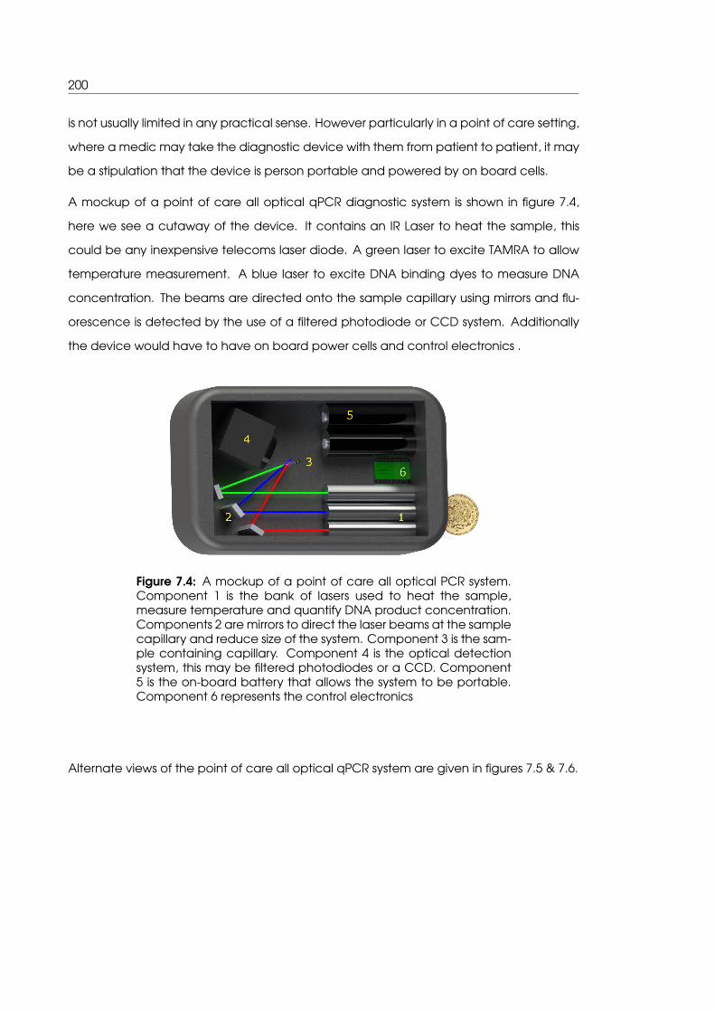
200
is not usually limited in any practical sense. However particularly in a point of care setting,
where a medic may take the diagnostic device with them from patient to patient, it may
be a stipulation that the device is person portable and powered by on board cells.
A mockup of a point of care all optical qPCR diagnostic system is shown in figure 7.4,
here we see a cutaway of the device. It contains an IR Laser to heat the sample, this
could be any inexpensive telecoms laser diode. A green laser to excite TAMRA to allow
temperature measurement. A blue laser to excite DNA binding dyes to measure DNA
concentration. The beams are directed onto the sample capillary using mirrors and flu-
orescence is detected by the use of a filtered photodiode or CCD system. Additionally
the device would have to have on board power cells and control electronics .
Figure 7.4: A mockup of a point of care all optical PCR system.Component 1 is the bank of lasers used to heat the sample,measure temperature and quantify DNA product concentration.Components 2 are mirrors to direct the laser beams at the samplecapillary and reduce size of the system. Component 3 is the sam-ple containing capillary. Component 4 is the optical detectionsystem, this may be filtered photodiodes or a CCD. Component5 is the on-board battery that allows the system to be portable.Component 6 represents the control electronics
Alternate views of the point of care all optical qPCR system are given in figures 7.5 & 7.6.
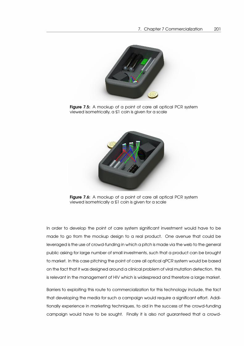
7. Chapter 7 Commercialization 201
Figure 7.5: A mockup of a point of care all optical PCR systemviewed isometrically, a £1 coin is given for a scale
Figure 7.6: A mockup of a point of care all optical PCR systemviewed isometrically a £1 coin is given for a scale
In order to develop the point of care system significant investment would have to be
made to go from the mockup design to a real product. One avenue that could be
leveraged is the use of crowd-funding in which a pitch is made via the web to the general
public asking for large number of small investments, such that a product can be brought
to market. In this case pitching the point of care all optical qPCR system would be based
on the fact that it was designed around a clinical problem of viral mutation detection. this
is relevant in the management of HIV which is widespread and therefore a large market.
Barriers to exploiting this route to commercialization for this technology include, the fact
that developing the media for such a campaign would require a significant effort. Addi-
tionally experience in marketing techniques, to aid in the success of the crowd-funding
campaign would have to be sought. Finally it is also not guaranteed that a crowd-

202
funding campaign would be able to generate sufficient funds to develop a point-of-care
system.
7.4 Summary of Commercialization strategy
In summation, the routes to commercialization and target market sectors for the technol-
ogy developed and presented in this thesis are as follows:
Development of licensing revenue streams from manufacturers of instrumentation for bio-
process monitoring. development of licensing revenue streams from Pharmaceutical firms
performing drug development operations.
Development of licensing revenue streams from manufacturers of qPCR machines. De-
veloping a crowd funding campaign for the production of a point of care all optical
qPCR device, this will be targeted at facilitating more rapid or even personal HIV disease
mutant detection.

203
Appendices

204

Appendix A. Single genome analysis week 0 consensus sequence 205
AppendixA. Single genome analysis
week 0 consensus sequenceCTGCTGGTGGCTCCAGTTCAGGAACACTCAACCCTGTTCCAAATATTGCCTCTCACATCTC
GTCAACCTCCTCGATAACTGGGGCCCCTGTGCCGAACATGGAGAACATCACATCAGG
ACTCCTAGGACCCCTGCTCGTGTTACAGGCGGGGTTTTTCTTGTTGACAAGAATCCTCACA
ATACCGCAGAGTCTAGACTCGTGGTGGACTTCTCTCAATTTTCTAGGGGGCACACCCGTG
TGTCTTGGCCAAAATTCGCAGTCCCCAACCTCCAATCACTCACCAACCTCCTGTCCTCC
AATTTGTCCTGGTTATCGCTGGATGTGTCTGCGGCGTTTTATCATATTCCTCTTCATCCTGCTGC
TATGCCTCATCTTCTTATTGGGTCTTCTGGATTGCAAAGGTATGTTACCCGTTTGTCCTATAATTC
CAGAATCCGCAACCACCAACAGGACACCCTGCAGGACCTGCACGACTCCTGCTCAA
GGCAACTCTATGTTACCCTCATGTTGCTGTACAAAACCTACGGATGGAAATTGCACTTGTA
TTCCCATCCCATCATCCTGGGCTTTCGCAAAATACCTATGGGAGTGGGTCTCAGCCCGTT
TCTCTTGGCTCAATTTACCAGTGCCATTTGTTCAGTGGTTCGGAGGGCATTCCCCCACTGTT
TGGCTTTCAGTTATATGGATGATGTGGTATTGGGGGCCAAGTCTGTACAACATCTTGAGTCC
CTTTATACCGCTGTTACCAATTTTCTTTTGTCTTTGGGTATACATTTAAACCCTAACAAAACAAA
AAGATGGGGTTATTCCCTAAACTTCATGGGATATGTAATTGGGAGTTGGGGTACATTGCCA
CAGGATCATATTGTACAAAAAATCAAACACTGTTTTAGAAAACTGCCTGTCAATCGACCTAT
TGATTGGAAAGTATGTCAAAGAATTGTGGGTCTTTTGGGCTTTGCCGCTCCATTTACACAATG
TGGTTACCCTGCTTTAATGCCTTTGTATGCCTGTATACAAGCGAAACAGGCTTTTACTTTCTCG
CCAACTTACAAGGCCTTTCTAAGTAAACAGTATATGAACCTTTACCCCGTTGCCCGGCAA
CGGCCTGGTCTGTGCCAAGTGTTTGCTGACGCAACCCCCACTGGCTGGGGCTTGGCC
ATCGGCCATCAGCGCATGCGCGGAACCTTTGTGGCTCCTCTGCCGATCCATACTGCGG
AACTCCT

206

Appendix B. sequencing data all sample genotype data 207
AppendixB. sequencing data all sample
genotype dataThese data were largely collected by Dr. Antonio Adrián González del Castillo with assis-
tance from me, they are from where the more succinct analysis in section 4.2 are derived,
and this is turn form the rationale for performing the rest of the analyses in Chapter 4.
the tables are split into three parts, firstly where only a sample for the first timepoint for
a patient was available, secondly where the first and second time points were avail-
able, thirdly where all three time points were available for a patient. The tables give
the the patient identifier then the HBV viral load for the patient at that time point given
in International Units/mL as measured using the qPCR protocol described earlier. Then
the genotype and mutational patterns in the reverse transcriptase and surface protein
open reading frames are given, as discerned by Sanger sequencing. Gaps in the charts
are when the data could not be obtained due to failure of either the qPCR protocol or
Sanger sequencing protocols, this in most cases is likely due to low viral load.
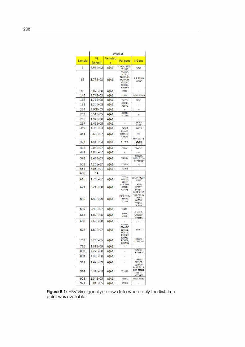
208
Figure B.1: HBV virus genotype raw data where only the first timepoint was available
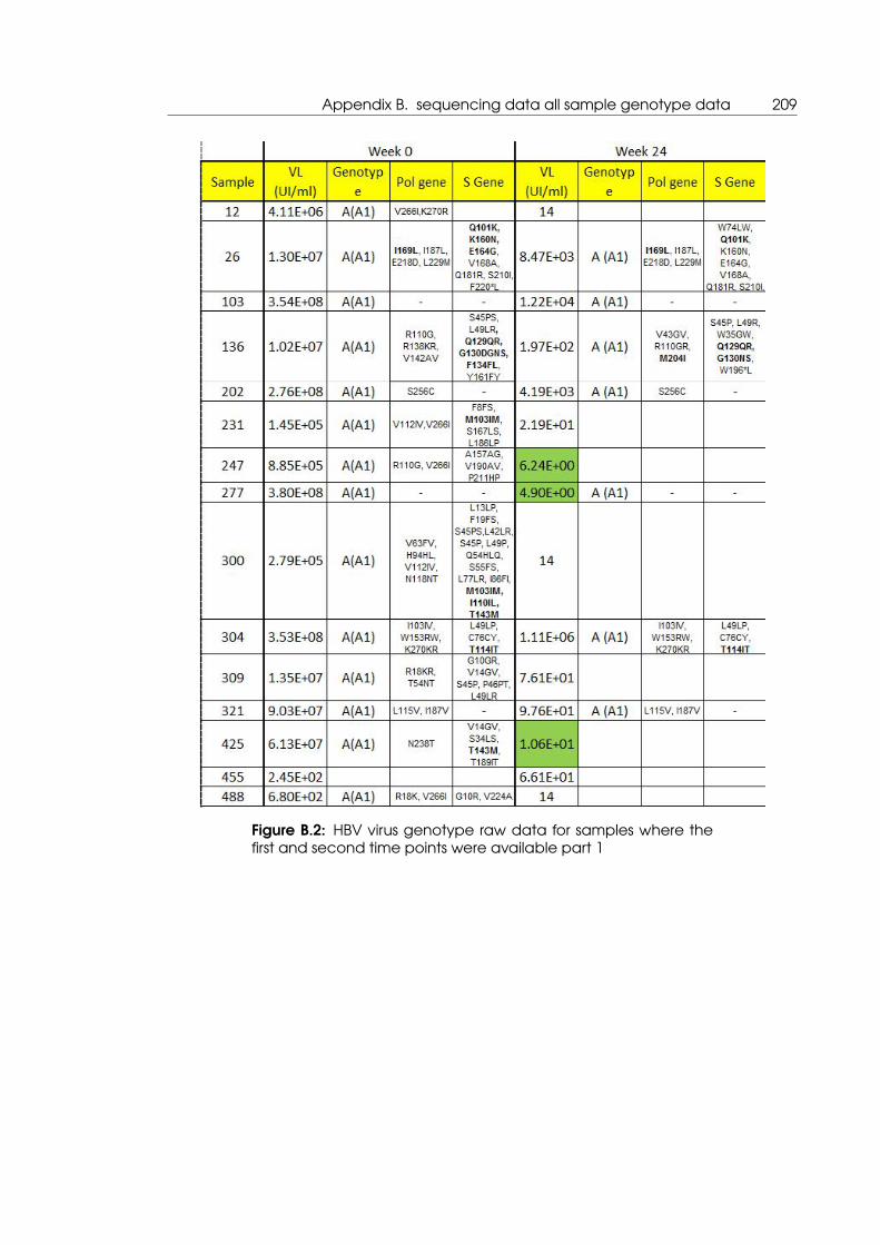
Appendix B. sequencing data all sample genotype data 209
Figure B.2: HBV virus genotype raw data for samples where thefirst and second time points were available part 1

210
Figure B.3: HBV virus genotype raw data for samples where thefirst and second time points were available part 2
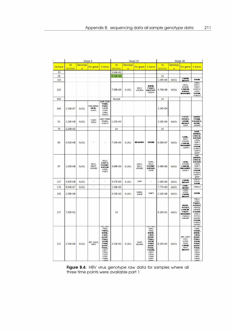
Appendix B. sequencing data all sample genotype data 211
Figure B.4: HBV virus genotype raw data for samples where allthree time points were available part 1

212
Figure B.5: HBV virus genotype raw data for samples where allthree time points were available part 2

3. Bibliography 213
3. Bibliography[Ahmed et al., 2010] Ahmed, T., Shimizu, T., and Stocker, R. (2010). Microfluidics for bac-
terial chemotaxis. Integrative Biology, 2:604–629.
[Alfano and Ockman, 1968] Alfano, R. R. and Ockman, N. (1968). Methods for detecting
weak light signals. Journal of the Optical Society of America, 58(1):90–93.
[Alivisatos, 1996] Alivisatos, A. (1996). Semiconductor clusters, nanocrystals, and quan-
tum dots. Science, 271(5251):933–937.
[Anfinsen et al., 1973] Anfinsen, C., Christian, B., et al. (1973). Principles that govern the
folding of protein chains. Science, 181(4096):223–230.
[Aoudjane et al., 2014] Aoudjane, S., Chaponda, M., del Castillo, A. A. G., O’Connor, J.,
Noguera, M., Beloukas, A., Hopkins, M., Khoo, S., van Oosterhout, J. J., and Geretti,
A. M. (2014). Hepatitis b virus sub-genotype a1 infection is characterized by high repli-
cation levels and rapid emergence of drug resistance in hiv-positive adults receiving
first-line antiretroviral therapy in malawi. Clinical Infectious Diseases, 59(11):1618–1626.
[Araujo et al., 2011] Araujo, N. M., Waizbort, R., and Kay, A. (2011). Hepatitis b virus in-
fection from an evolutionary point of view: how viral, host, and environmental factors
shape genotypes and subgenotypes. Infection, Genetics and Evolution, 11(6):1199–
1207.
[Aström and Murray, 2010] Aström, K. J. and Murray, R. M. (2010). Feedback systems: an
introduction for scientists and engineers. Princeton university press.
[Aucamp et al., 2005] Aucamp, J. P., Cosme, A. M., Lye, G. J., and Dalby, P. A. (2005).
High-throughput measurement of protein stability in microtiter plates. Biotechnology
and Bioengineering, 89(5):599–607.
[Aucamp et al., 2008] Aucamp, J. P., Martinez-Torres, R. J., Hibbert, E. G., and Dalby, P. A.
(2008). A microplate-based evaluation of complex denaturation pathways: Struc-
tural stability of escherichia coli transketolase. Biotechnology and Bioengineering,
99(6):1303–1310.
[Baaske et al., 2007] Baaske, P., Duhr, S., and Braun, D. (2007). Melting curve analysis in a
snapshot. Applied Physics Letters, 91(13):133901.

214
[Baffou et al., 2012] Baffou, G., Bon, P., Savatier, J., Polleux, J., Zhu, M., Merlin, M.,
Rigneault, H., and Monneret, S. (2012). Thermal imaging of nanostructures by quan-
titative optical phase analysis. ACS Nano, 6(3):2452–2458.
[Ballantyne et al., 2008] Ballantyne, K. N., Van Oorschot, R. A. H., and Mitchell, R. J. (2008).
Locked nucleic acids in pcr primers increase sensitivity and performance. Genomics,
91(3):301–305.
[Bartholomeusz and Locarnini, 2006] Bartholomeusz, A. and Locarnini, S. (2006). Hepati-
tis b virus mutations associated with antiviral therapy. Journal of Medical Virology,
78(S1):S52–S55.
[Beck and Nassal, 2007] Beck, J. and Nassal, M. (2007). Hepatitis b virus replication. World
journal of gastroenterology, 13(1):48.
[Beck et al., 2002] Beck, J., Vogel, M., and Nassal, M. (2002). dntp versus ntp discrimi-
nation by phenylalanine 451 in duck hepatitis b virus p protein indicates a common
structure of the dntp-binding pocket with other reverse transcriptases. Nucleic Acids
Research, 30(7):1679–1687.
[Belgrader et al., 2000] Belgrader, P., Okuzumi, M., Pourahmadi, F., Borkholder, D. A., and
Northrup, M. A. (2000). A microfluidic cartridge to prepare spores for pcr analysis.
Biosensors and Bioelectronics, 14(10):849–852.
[Bernas et al., 2004] Bernas, T., Zabreski, M., Cook, R. R., and Dobrucki, J. (2004). Mini-
mizing photobleaching during confocal microscopy of fluorescent probes bound to
chromatin: role of anoxia and photon flux. Journal of Microscopy, 215(3):281–296.
[Bokman and Ward, 1981] Bokman, S. H. and Ward, W. W. (1981). Renaturation of ae-
quorea green-fluorescent protein. Biochemical and biophysical research communica-
tions, 101(4):1372–1380.
[Boyer et al., 2011] Boyer, T. D., Wright, T. L., and Manns, M. P. (2011). Zakim and Boyer’s
hepatology: a textbook of liver disease. Elsevier Health Sciences.
[Brancaleon et al., 1999] Brancaleon, L., Lin, G., and Kollias, N. (1999). The in vivo fluores-
cence of tryptophan moieties in human skin increases with uv exposure and is a marker
for epidermal proliferation. Journal of Investigative Dermatology, 113(6):977–982.

3. Bibliography 215
[Brandts and Lin, 1990] Brandts, J. F. and Lin, L. N. (1990). Study of strong to ultratight
protein interactions using differential scanning calorimetry. Biochemistry, 29(29):6927–
6940.
[Braun, 2004] Braun, D. (2004). Pcr by thermal convection. Modern Physics Letters B,
18(16):775–784.
[Braun et al., 2003] Braun, D., Goddard, N. L., and Libchaber, A. (2003). Exponential dna
replication by laminar convection. Physical Review Letters, 91(15):158103.
[Brites et al., 2011] Brites, C. D., Lima, P. P., Silva, N. J., Millán, A., Amaral, V. S., Palacio, F.,
and Carlos, L. D. (2011). Lanthanide-based luminescent molecular thermometers. New
Journal of Chemistry, 35(6):1177–1183.
[Brites et al., 2012] Brites, C. D. S., Lima, P. P., Silva, N. J., Millán, A., Amaral, V. S., Palacio, F.,
and Carlos, L. D. (2012). Thermometry at the nanoscale. Nanoscale, 4(16):4799–4829.
[Capobianchi et al., 2013] Capobianchi, M. R., Giombini, E., and Rozera, G. (2013). Next-
generation sequencing technology in clinical virology. Clinical Microbiology and Infec-
tion, 19(1):15–22.
[Carey and Harrison, 2009] Carey, I. and Harrison, P. M. (2009). Monotherapy versus com-
bination therapy for the treatment of chronic hepatitis b. Expert Opinion on Investiga-
tional Drugs, 18(11):1655–1666.
[Chalfie et al., 1994] Chalfie, M., Tu, Y., Euskirchen, G., Ward, W. W., and Prasher, D. C.
(1994). Green fluorescent protein as a marker for gene expression. Science,
263(5148):802–805.
[Chatterjea and Shinde, 2011] Chatterjea, M. N. and Shinde, R. (2011). Textbook of Med-
ical Biochemistry. Wife Goes On.
[Chen et al., 2000] Chen, C.-J., Wang, L.-Y., and Yu, M.-W. (2000). Epidemiology of hep-
atitis b virus infection in the asia–pacific region. Journal of Gastroenterology and Hep-
atology, 15(s2):E3–E6.
[Cheng et al., 1996] Cheng, J., Shoffner, M. A., Hvichia, G. E., Kricka, L. J., and Wilding,
P. (1996). Chip pcr. ii. investigation of different pcr amplification systems in microfabri-
cated silicon-glass chips. Nucleic Acids Research, 24(2):380–385.

216
[Christie and Bryant, 2005] Christie, R. M. and Bryant, I. D. (2005). An evaluation of ther-
mochromic prints based on microencapsulated liquid crystals using variable tempera-
ture colour measurement. Coloration Technology, 121(4):187–192.
[Chun et al., 2012] Chun, H. M., Roediger, M. P., Hullsiek, K. H., Thio, C. L., Agan, B. K.,
Bradley, W. P., Peel, S. A., Jagodzinski, L. L., Weintrob, A. C., Ganesan, A., et al. (2012).
Hepatitis b virus coinfection negatively impacts hiv outcomes in hiv seroconverters.
Journal of Infectious Diseases, 205(2):185–193.
[Cirino et al., 2003] Cirino, P. C., Mayer, K. M., and Umeno, D. (2003). Generating mu-
tant libraries using error-prone pcr. In Directed Evolution Library Creation, pages 3–9.
Springer.
[Cohen, 2011] Cohen, J. (2011). Halting hiv/aids epidemics.
[Cosa et al., 2001] Cosa, G., Focsaneanu, K.-S., McLean, J. R. N., McNamee, J. P., and
Scaiano, J. C. (2001). Photophysical properties of fluorescent dna-dyes bound to single-
and double-stranded dna in aqueous buffered solution. Photochemistry and Photobi-
ology, 73(6):585–599.
[Dane et al., 1970] Dane, D. S., Cameron, C. H., and Briggs, M. (1970). Virus-like par-
ticles in serum of patients with australia-antigen-associated hepatitis. The Lancet,
295(7649):695–698.
[Deny and Zoulim, 2010] Deny, P. and Zoulim, F. (2010). Hepatitis b virus: from diagnosis to
treatment. Pathologie Biologie, 58(4):245–253.
[Drexhage, 1973] Drexhage, K. H. (1973). What’s ahead in laser dyes. Laser Focus,
9(3):35–39.
[education, 2010] education, N. (2010). The composition of a bacterial cell. Nature Pub-
lishing group.
[Eggeling et al., 1998] Eggeling, C., Widengren, J., Rigler, R., and Seidel, C. A. M. (1998).
Photobleaching of fluorescent dyes under conditions used for single-moleculeole de-
tection: evidence of two-step photolysis. Analytical Chemistry, 70(13):2651–2659.
[Fan and Longtin, 2000] Fan, C. H. and Longtin, J. P. (2000). Laser-based measurement of
liquid temperature or concentration at a solid liquid interface. Experimental Thermal
and Fluid Science, 23(12):1 – 9.
3. Bibliography 217
[Fersht, 1999] Fersht, A. (1999). Structure and mechanism in protein science: a guide to
enzyme catalysis and protein folding. Macmillan.
[Findlay et al., 1993] Findlay, J. B., Atwood, S. M., Bergmeyer, L., Chemelli, J., Christy, K.,
Cummins, T., Donish, W., Ekeze, T., Falvo, J., and Patterson, D. (1993). Automated closed-
vessel system for in vitro diagnostics based on polymerase chain reaction. Clinical
Chemistry, 39(9):1927–1933.
[Fraser et al., 2016] Fraser, N. J., Liu, J. W., Mabbitt, P. D., Correy, G., Coppin, C. W., Lethier,
M., Perugini, M. A., Murphy, J. M., Oakeshott, J. G., Weik, M., et al. (2016). Evolution of
protein quaternary structure in response to selective pressure for increased thermosta-
bility. Journal of Molecular Biology.
[Freed and Mouland, 2006] Freed, E. O. and Mouland, A. J. (2006). The cell biology of
hiv-1 and other retroviruses. Retrovirology, 3(1):77.
[Freitas, 1998] Freitas, R. A. (1998). Nanomedicine. Foresight institute.
[Gallego et al., 2011] Gallego, L., Barreiro, P., and Lopéz-Ibor, J. J. (2011). Diagnosis and
clinical features of major neuropsychiatric disorders in hiv infection. AIDS Reviews,
13(3):171–9.
[Gallery et al., 1994] Gallery, J., Gouterman, M., Callis, J., Khalil, G., McLachlan, B., and
Bell, J. (1994). Luminescent thermometry for aerodynamic measurements. Review of
Scientific Instruments, 65(3):712–720.
[Ganem and Prince, 2004] Ganem, D. and Prince, A. M. (2004). Hepatitis b virus infec-
tion natural history and clinical consequences. New England Journal of Medicine,
350(11):1118–1129.
[Gaudet et al., 2010] Gaudet, M., Remtulla, N., Jackson, S. E., Main Ewan, R. G.,
Bracewell, D. G., Aeppli, G., Dalby, P. A., et al. (2010). Protein denaturation and pro-
tein: drugs interactions from intrinsic protein fluorescence measurements at the nano-
litre scale. Protein Science, 19(8):1544–1554.
[Giordano et al., 2001] Giordano, B. C., Ferrance, J., Swedberg, S., Hühmer, A. F. R., and
Landers, J. P. (2001). Polymerase chain reaction in polymeric microchips: Dna amplifi-
cation in less than 240 seconds. Analytical Biochemistry, 291(1):124–132.
[Goldys, 2009] Goldys, E. M. (2009). Fluorescence applications in biotechnology and life
sciences. John Wiley & Sons.
218
[Gossett et al., 2010] Gossett, D. R., Weaver, W. M., Mach, A. J., Hur, S. C., Tse, H. T. K.,
Lee, W., Amini, H., and Di Carlo, D. (2010). Label-free cell separation and sorting in
microfluidic systems. Analytical and Bioanalytical Chemistry, 397(8):3249–3267.
[Greenleaf and Sidow, 2014] Greenleaf, W. J. and Sidow, A. (2014). The future of se-
quencing: convergence of intelligent design and market darwinism. Genome Biology,
15(3):303.
[Grodzinski et al., 2001] Grodzinski, P., Liu, R. H., Chen, B., Blackwell, J., Liu, Y., Rhine, D.,
Smekal, T., Ganser, D., Romero, C., Yu, H., et al. (2001). Development of plastic mi-
crofluidic devices for sample preparation. Biomedical Microdevices, 3(4):275–283.
[Guilbault, 1990] Guilbault, G. G. (1990). Practical Fluorescence, Second Edition. Number
page number 79 in Modern Monographs in Analytical Chemistry. Taylor & Francis.
[Haché and Villeneuve, 2006] Haché, C. and Villeneuve, J.-P. (2006). Lamivudine treat-
ment in patients with chronic hepatitis b and cirrhosis. Expert Opinion on Pharma-
cotherapy, 7(13):1835–43.
[Hale and Querry, 1973] Hale, G. M. and Querry, M. R. (1973). Optical constants of water
in the 200-nm to 200-µm wavelength region. Applied Optics, 12(3):555–563.
[Hansen and Khanna, 2004] Hansen, K. and Khanna, C. (2004). Spontaneous and genet-
ically engineered animal models: use in preclinical cancer drug development. Euro-
pean Journal of Cancer, 40(6):858–880.
[Hau et al., 2011] Hau, J. C., Fontana, P., Zimmermann, C., De Pover, A., Erdmann, D.,
and Chène, P. (2011). Leveraging the contribution of thermodynamics in drug discov-
ery with the help of fluorescence-based thermal shift assays. Journal of Biomolecular
Screening, 16(5):552–556.
[Hawkins, ] Hawkins, K. Soldier deploys to iraq to help field laser defense system for chi-
nook helicopters.
[He et al., 2001] He, Y., Zhang, Y. H., and Yeung, E. S. (2001). Capillary-based fully inte-
grated and automated system for nanoliter polymerase chain reaction analysis directly
from cheek cells. Journal of Chromatography A, 924(1):271–284.
[Herschhorn and Hizi, 2010] Herschhorn, A. and Hizi, A. (2010). Retroviral reverse transcrip-
tases. Cellular and Molecular Life Sciences, 67(16):2717–2747.
3. Bibliography 219
[Higuchi et al., 1993] Higuchi, R., Fockler, C., Dollinger, G., and Watson, R. (1993). Kinetic
pcr analysis: real-time monitoring of dna amplification reactions. Nature Biotechnol-
ogy, (11):1026–30.
[Hoang et al., 2008] Hoang, V. N., Kaigala, G. V., and Backhouse, C. J. (2008). Dynamic
temperature measurement in microfluidic devices using thermochromic liquid crystals.
Lab on a Chip, 8(3):484–487.
[Hodko et al., 2001] Hodko, D., Raymer, L., Herbst, S. M., Magnuson, J. W., and Gaskin,
D. (2001). Detection of pathogens using on-chip electrochemical analysis of pcr am-
plified dna molecules. BiOS 2001 The International Symposium on Biomedical Optics,
4265:65–74.
[Hsieh et al., 2008] Hsieh, T.-M., Luo, C.-H., Huang, F.-C., Wang, J.-H., Chien, L.-J., and Lee,
G.-B. (2008). Enhancement of thermal uniformity for a microthermal cycler and its ap-
plication for polymerase chain reaction. Sensors and Actuators B: Chemical, 130(2):848
– 856.
[Hu and Liu, 2010] Hu, J. and Liu, S. (2010). Responsive polymers for detection and sensing
applications: current status and future developments. Macromolecules, 43(20):8315–
8330.
[Hughes et al., 2011] Hughes, J., Rees, S., Kalindjian, S. B., and Philpott, K. L. (2011). Princi-
ples of early drug discovery. British Journal of Pharmacology, 162(6):1239–1249.
[Hühmer and Landers, 2000] Hühmer, A. F. R. and Landers, J. P. (2000). Noncontact
infrared-mediated thermocycling for effective polymerase chain reaction amplifica-
tion of dna in nanoliter volumes. Analytical Chemistry, 72(21):5507–5512.
[Hutchison, 2007] Hutchison, C. A. (2007). Dna sequencing: bench to bedside and be-
yond. Nucleic Acids Research, 35(18):6227–6237.
[Hwang and Cheung, 2011] Hwang, E. W. and Cheung, R. (2011). Global epidemiology
of hepatitis b virus (hbv) infection. North American Journal of Medical Sciences, 4(1):7–
13.
[Ibrahim et al., 1998] Ibrahim, M. S., Lofts, R. S., Jahrling, P. B., Henchal, E. A., Weedn, V. W.,
Northrup, M. A., and Belgrader, P. (1998). Real-time microchip pcr for detecting single-
base differences in viral and human dna. Analytical Chemistry, 70(9):2013–2017.

220
[Ismail et al., 2014] Ismail, A. M., Ramachandran, J., Kannangai, R., Abraham, P., et al.
(2014). Antiviral efficacy of adefovir dipivoxil in the treatment of chronic hepatitis b
subjects from indian subcontinent. Indian Journal of Medical Microbiology, 32(1):60.
[Jones et al., 1999] Jones, S. F., Evans, G. M., and Galvin, K. P. (1999). Bubble nucleation
from gas cavities a review. Advances in Colloid and Interface Science, 80(1):27 – 50.
[Jung et al., 2011] Jung, H., Hoang, V. N., Gusev, E., Baek, H., Wang, Y., and Diebold, G. J.
(2011). Ludwig soret effect in a linear temperature field: Theory and experiments for
steady state distributions. Physics Letters A, 375(19):1917 – 1920.
[Kemnitz et al., 1989] Kemnitz, K., Nakashima, N., Yoshihara, K., and Matsunami, H.
(1989). Temperature dependence of fluorescence decays of isolated rhodamine b
molecules adsorbed on semiconductor single crystals. The Journal of Physical Chem-
istry, 93(18):6704–6710.
[Khandurina et al., 2000] Khandurina, J., McKnight, T. E., Jacobson, S. C., Waters, L. C.,
Foote, R. S., and Ramsey, J. M. (2000). Integrated system for rapid pcr-based dna
analysis in microfluidic devices. Analytical Chemistry, 72(13):2995–3000.
[Kim et al., 2013] Kim, D. Y., Chang, H. Y., Lim, S. M., Kim, S. U., Park, J. Y., Kim, J. K., Lee,
K. S., Han, K.-H., Chon, C. Y., and Ahn, S. H. (2013). Quasispecies and pre-existing drug-
resistant mutations of hepatitis b virus in patients with chronic hepatitis b. Gut and Liver,
7(3):329–334.
[Kim et al., 2009a] Kim, H., Dixit, S., Green, C. J., and Faris, G. W. (2009a). Nanodroplet
real-time pcr system with laser assisted heating. Optics Express, 17(1):218–227.
[Kim et al., 2009b] Kim, H., Vishniakou, S., and Faris, G. W. (2009b). Petri dish pcr: laser-
heated reactions in nanoliter droplet arrays. Lab on a Chip, 9(9):1230–1235.
[Kim et al., 2006] Kim, S. H., Noh, J., Jeon, M. K., Kim, K. W., Lee, L. P., and Woo, S. I. (2006).
Micro-raman thermometry for measuring the temperature distribution inside the mi-
crochannel of a polymerase chain reaction chip. Journal of Micromechanics and
Microengineering, 16(3):526.
[Kirk et al., 2002] Kirk, O., Borchert, T. V., and Fuglsang, C. C. (2002). Industrial enzyme
applications. Current Opinion in Biotechnology, 13(4):345–351.
3. Bibliography 221
[Kucsko et al., 2013] Kucsko, G., Maurer, P. C., Yao, N. Y., Kubo, M., Noh, H. J., Lo, P. K.,
Park, H., and Lukin, M. D. (2013). Nanometre-scale thermometry in a living cell. Nature,
500(7460):54–58.
[Lagally et al., 2000] Lagally, E. T., Simpson, P. C., and Mathies, R. A. (2000). Monolithic
integrated microfluidic dna amplification and capillary electrophoresis analysis system.
Sensors and Actuators B: Chemical, 63(3):138–146.
[Lai et al., 1998] Lai, C.-L., Chien, R.-N., Leung, N. W. Y., Chang, T.-T., Guan, R., Tai, D.-I., Ng,
K.-Y., Wu, P.-C., Dent, J. C., Barber, J., et al. (1998). A one-year trial of lamivudine for
chronic hepatitis b. New England Journal of Medicine, 339(2):61–68.
[Lakowicz, 2007] Lakowicz, J. R. (2007). Principles of Fluorescence Spectroscopy. Springer.
[Lavanchy, 2004] Lavanchy, D. (2004). Hepatitis b virus epidemiology, disease burden,
treatment, and current and emerging prevention and control measures. Journal of
Viral Hepatitis, 11(2):97–107.
[Lavinder et al., 2009] Lavinder, J. J., Hari, S. B., Sullivan, B. J., and Magliery, T. J. (2009).
High-throughput thermal scanning: a general, rapid dye-binding thermal shift screen
for protein engineering. Journal of the American Chemical Society, 131(11):3794–3795.
[Lee, 1997] Lee, W. M. (1997). Hepatitis b virus infection. New England Journal of
Medicine, 337(24):1733–1745.
[Leiderman et al., 2006] Leiderman, P., Huppert, D., and Agmon, N. (2006). Transition in
the temperature-dependence of gfp fluorescence: from proton wires to proton exit.
Biophysical Journal, 90(3):1009–1018.
[Li et al., 2007] Li, S., Zhang, K., Yang, J.-M., Lin, L., and Yang, H. (2007). Single quantum
dots as local temperature markers. Nano Letters, 7(10):3102–3105.
[Libbrecht et al., 2007] Libbrecht, E., Doutreloigne, J., Van De Velde, H., Yuen, M.-F., Lai,
C.-L., Shapiro, F., and Sablon, E. (2007). Evolution of primary and compensatory lamivu-
dine resistance mutations in chronic hepatitis b virus-infected patients during long-term
lamivudine treatment, assessed by a line probe assay. Journal of Clinical Microbiology,
45(12):3935–3941.
[Lin and Kao, 2011] Lin, C.-L. and Kao, J.-H. (2011). The clinical implications of hepatitis
b virus genotype: Recent advances. Journal of Gastroenterology and Hepatology,
26:123–130.
222
[Livinson, 1949] Livinson, R. (1949). Irreversible and reversible photobleaching of dyes.
Journal of the Society of Dyers and Colourists, 65(12):781–785.
[Lok et al., 2007] Lok, A. S., Zoulim, F., Locarnini, S., Bartholomeusz, A., Ghany, M. G.,
Pawlotsky, J.-M., Liaw, Y.-F., Mizokami, M., and Kuiken, C. (2007). Antiviral drug-resistant
hbv: Standardization of nomenclature and assays and recommendations for manage-
ment. Hepatology, 46(1):254–265.
[Lok and McMahon, 2009] Lok, A. S. F. and McMahon, B. J. (2009). Chronic hepatitis b:
update 2009. Hepatology, 50(3):661–662.
[Lou et al., 1999] Lou, J., Finegan, T. M., Mohsen, P., Hatton, T. A., and Laibinis, P. E. (1999).
Fluorescence-based thermometry: principles and applications. Reviews in Analytical
Chemistry, 18(4):235–284.
[Mahon et al., 2014] Mahon, C. R., Lehman, D. C. C., and Manuselis Jr, G. (2014). Text-
book of diagnostic microbiology. Elsevier Health Sciences.
[Makhatadze and Privalov, 1990] Makhatadze, G. I. and Privalov, P. L. (1990). Heat ca-
pacity of proteins: I. partial molar heat capacity of individual amino acid residues in
aqueous solution: Hydration effect. Journal of Molecular Biology, 213(2):375 – 384.
[Maltezos et al., 2008] Maltezos, G., Gomez, A., Zhong, J., Gomez, F. A., and Scherer, A.
(2008). Microfluidic polymerase chain reaction. Applied Physics Letters, 93(24):243901.
[Manz et al., 1990] Manz, A., Graber, N., and Widmer, H. M. (1990). Miniaturized total
chemical analysis systems: A novel concept for chemical sensing. Sensors and Actua-
tors B: Chemical, 1(16):244 – 248.
[Manz et al., 1992] Manz, A., Harrison, D. J., Verpoorte, E. M. J., Fettinger, J. C., Paulus,
A., Lüdi, H., and Widmer, H. M. (1992). Planar chips technology for miniaturization and
integration of separation techniques into monitoring systems: Capillary electrophoresis
on a chip. Journal of Chromatography A, 593(12):253 – 258.
[Margeridon-Thermet et al., 2009] Margeridon-Thermet, S., Shulman, N. S., Ahmed, A.,
Shahriar, R., Liu, T., Wang, C., Holmes, S. P., Babrzadeh, F., Gharizadeh, B., Hanczaruk,
B., Simen, B. B., Egholm, M., and Shafer, R. W. (2009). Ultra-deep pyrosequencing of
hepatitis b virus quasispecies from nucleoside and nucleotide reverse-transcriptase in-
hibitor (nrti)-treated patients and nrti-naive patients. Journal of Infectious Diseases,
199(9):1275–1285.

3. Bibliography 223
[Margulies et al., 2005] Margulies, M., Egholm, M., Altman, W. E., Attiya, S., Bader, J. S.,
Bemben, L. A., Berka, J., Braverman, M. S., Chen, Y.-J., Chen, Z., et al. (2005). Genome
sequencing in microfabricated high-density picolitre reactors. Nature, 437(7057):376–
380.
[Metzker and Caskey, 2001] Metzker, M. L. and Caskey, C. T. (2001). Polymerase Chain
Reaction (PCR). John Wiley & Sons, Ltd.
[Milich et al., 1998] Milich, D. R., Chen, M. K., Hughes, J. L., and Jones, J. E. (1998). The se-
creted hepatitis b precore antigen can modulate the immune response to the nucle-
ocapsid: a mechanism for persistence. The Journal of Immunology, 160(4):2013–2021.
[Miller, 1924] Miller, C. C. (1924). The stokes-einstein law for diffusion in solution. Proceed-
ings of the Royal Society of London. Series A, Containing Papers of a Mathematical
and Physical Character, 106(740):724–749.
[Mueller et al., 2000] Mueller, O., Hahnenberger, K., Dittmann, M., Yee, H., Dubrow, R.,
Nagle, R., and Ilsley, D. (2000). A microfluidic system for high-speed reproducible dna
sizing and quantitation. Electrophoresis, 21(1):128–134.
[Mullineaux et al., 2006] Mullineaux, C. W., Nenninger, A., Ray, N., and Robinson, C.
(2006). Diffusion of green fluorescent protein in three cell environments in escherichia
coli. Journal of bacteriology, 188(10):3442–3448.
[Mullis et al., 1992] Mullis, K. B., Faloona, F. A., Scharf, S. J., Saiki, R. K., Horn, G. T., and
Erlich, H. (1992). Specific enzymatic amplification of dna in vitro: the polymerase chain
reaction. Biotechnology Series, pages 17–17.
[Neumann et al., 2013] Neumann, P., Jakobi, I., Dolde, F., Burk, C., Reuter, R., Waldherr,
G., Honert, J., Wolf, T., Brunner, A., Shim, J. H., et al. (2013). High-precision nanoscale
temperature sensing using single defects in diamond. Nano Letters, 13(6):2738–2742.
[Ngui and Teo, 1997] Ngui, S. L. and Teo, C. G. (1997). Hepatitis b virus genomic hetero-
geneity: variation between quasispecies may confound molecular epidemiological
analyses of transmission incidents. Journal of Viral Hepatitis, 4(5):309–315.
[Niesen et al., 2007] Niesen, F. H., Berglund, H., and Vedadi, M. (2007). The use of differ-
ential scanning fluorimetry to detect ligand interactions that promote protein stability.
Nature Protocols, 2(9):2212–2221.
224
[Northrup et al., 1995] Northrup, M. A., Gonzalez, C., Lehew, S., and Hills, R. (1995). Devel-
opment of a pcr-microreactor. In Micro total analysis systems, pages 139–139. Springer.
[Nyirenda et al., 2008] Nyirenda, M., Beadsworth, M. B. J., Stephany, P., Hart, C. A., Hart,
I. J., Munthali, C., Beeching, N. J., and Zijlstra, E. E. (2008). Prevalence of infection with
hepatitis b and c virus and coinfection with hiv in medical inpatients in malawi. Journal
of Infection, 57(1):72–77.
[Oda et al., 1998] Oda, R. P., Strausbauch, M. A., Huhmer, A. F. R., Borson, N., Jurrens, S. R.,
Craighead, J., Wettstein, P. J., Eckloff, B., Kline, B., and Landers, J. (1998). Infrared-
mediated thermocycling for ultrafast polymerase chain reaction amplification of dna.
Analytical Chemistry, 70(20):4361–4368.
[Ormo et al., 1996] Ormo, M., Cubitt, A. B., Kallio, K., Gross, L. A., Tsien, R. Y., and Reming-
ton, S. J. (1996). Crystal structure of the aequorea victoria green fluorescent protein.
Science, 273(5280):1392–1395.
[Osborne, 1919] Osborne, T. B. (1919). The vegetable proteins. Longmans, Green, and
Company.
[Overington et al., 2006] Overington, J. P., Al-Lazikani, B., and Hopkins, A. L. (2006). How
many drug targets are there? Nature Reviews Drug discovery, 5(12):993–996.
[Pantoliano et al., 2001] Pantoliano, M. W., Petrella, E. C., Kwasnoski, J. D., Lobanov, V. S.,
Myslik, J., Graf, E., Carver, T., Asel, E., Springer, B. A., Lane, P., et al. (2001). High-density
miniaturized thermal shift assays as a general strategy for drug discovery. Journal of
Biomolecular Screening, 6(6):429–440.
[Price et al., 2009] Price, M. N., Dehal, P. S., and Arkin, A. P. (2009). Fasttree: computing
large minimum evolution trees with profiles instead of a distance matrix. Molecular
Biology and Evolution, 26(7):1641–1650.
[Pujol et al., 2009] Pujol, F. H., Navas, M.-C., Hainaut, P., and Chemin, I. (2009). Worldwide
genetic diversity of hbv genotypes and risk of hepatocellular carcinoma. Cancer Let-
ters, 286(1):80–88.
[Ravey et al., 2012] Ravey, C., Pradere, C., Regnier, N., and Batsale, J.-C. (2012). New
temperature field processing from ir camera for velocity, thermal diffusivity and calori-
metric non-intrusive measurements in microfluidics systems. Quantitative InfraRed Ther-
mography Journal, 9(1):79–98.
3. Bibliography 225
[Rawat et al., 2012] Rawat, S., Clippinger, A. J., and Bouchard, M. J. (2012). Modulation
of apoptotic signaling by the hepatitis b virus x protein. Viruses, 4(11):2945–2972.
[Rehermann and Nascimbeni, 2005] Rehermann, B. and Nascimbeni, M. (2005). Im-
munology of hepatitis b virus and hepatitis c virus infection. Nature Reviews Immunol-
ogy, 5(3):215–229.
[Robertson and Murphy, 1997] Robertson, A. D. and Murphy, K. P. (1997). Protein structure
and the energetics of protein stability. Chemical Reviews, 97(5):1251–1268.
[Rodriguez-Frias et al., 2013] Rodriguez-Frias, F., Buti, M., Tabernero, D., and Homs, M.
(2013). Quasispecies structure, cornerstone of hepatitis b virus infection: Mass sequenc-
ing approach. World journal of gastroenterology: WJG, 19(41):6995.
[Romano et al., 1989] Romano, V., Zweig, A. D., Frenz, M., and Weber, H. P. (1989). Time-
resolved thermal microscopy with fluorescent films. Applied Physics B, 49(6):527–533.
[Ronaghi, 2001] Ronaghi, M. (2001). Pyrosequencing sheds light on dna sequencing.
Genome Research, 11(1):3–11.
[Ross et al., 2001] Ross, D., Gaitan, M., and Locascio, L. E. (2001). Temperature measure-
ment in microfluidic systems using a temperature-dependent fluorescent dye. Analyti-
cal Chemistry, 73(17):4117–4123.
[Rozing et al., 2001] Rozing, G., Serwe, M., Weissgerber, H.-G., and Glatz, B. (2001). A
system and columns for capillary hplc. American Laboratory, 33(10):26–39.
[Sackett and Cook, 1994] Sackett, D. L. and Cook, R. J. (1994). Understanding clinical
trials. BMJ: British Medical Journal, 309(6957):755.
[Sackmann et al., 2014] Sackmann, E. K., Fulton, A. L., and Beebe, D. J. (2014). The
present and future role of microfluidics in biomedical research. Nature, 507(7491):181–
189.
[Sakakibara et al., 1993] Sakakibara, J., Hishida, K., and Maeda, M. (1993). Measure-
ments of thermally stratified pipe flow using image-processing techniques. Experiments
in Fluids, 16(2):82–96.
[Sanger and Coulson, 1975] Sanger, F. and Coulson, A. R. (1975). A rapid method for
determining sequences in dna by primed synthesis with dna polymerase. Journal of
Molecular Biology, 94(3):441–448.

226
[Sanseau et al., 2012] Sanseau, P., Agarwal, P., Barnes, M. R., Pastinen, T., Richards, J. B.,
Cardon, L. R., and Mooser, V. (2012). Use of genome-wide association studies for drug
repositioning. Nature Biotechnology, 30(4):317–320.
[Sauer et al., 2010] Sauer, M., Hofkens, J., and Enderlein, J. (2010). Handbook of fluores-
cence spectroscopy and imaging: from ensemble to single molecules. John Wiley &
Sons.
[Saunders et al., 2013] Saunders, C. D., Holst, G. L., Phaneuf, C. R., Pak, N., Marchese,
M., Sondej, N., McKinnon, M., and Forest, C. R. (2013). Rapid, quantitative, reverse
transcription pcr in a polymer microfluidicchip. Biosensors and Bioelectronics, 44:222–
228.
[Schädler and Hildt, 2009] Schädler, S. and Hildt, E. (2009). Hbv life cycle: entry and mor-
phogenesis. Viruses, 1(2):185–209.
[Schmid et al., 2001] Schmid, A., Dordick, J. S., Hauer, B., Kiener, A., Wubbolts, M., and
Witholt, B. (2001). Industrial biocatalysis today and tomorrow. Nature, 409(6817):258–
268.
[Schrader et al., 2012] Schrader, C., Schielke, A., Ellerbroek, L., and Johne, R. (2012).
Pcr inhibitors occurrence, properties and removal. Journal of Applied Microbiology,
113(5):1014–1026.
[Shah et al., 2009] Shah, J. J., Gaitan, M., and Geist, J. (2009). Generalized temperature
measurement equations for rhodamine b dye solution and its application to microflu-
idics. Analytical Chemistry, 81(19):8260–8263.
[Sheldon et al., 2007] Sheldon, J., Ramos, B., Garcia-Samaniego, J., Rios, P.,
Bartholomeusz, A., Romero, M., Locarnini, S., Zoulim, F., and Soriano, V. (2007).
Selection of hepatitis b virus (hbv) vaccine escape mutants in hbv-infected and
hbv/hiv-coinfected patients failing antiretroviral drugs with anti-hbv activity. JAIDS
Journal of Acquired Immune Deficiency Syndromes, 46(3):279–282.
[Sheldon and Soriano, 2008] Sheldon, J. and Soriano, V. (2008). Hepatitis b virus es-
cape mutants induced by antiviral therapy. Journal of Antimicrobial Chemotherapy,
61(4):766–768.
[Shendure and Ji, 2008] Shendure, J. and Ji, H. (2008). Next-generation dna sequencing.
Nature Biotechnology, 26(10):1135–1145.

3. Bibliography 227
[Shoffner et al., 1996] Shoffner, M. A., Cheng, J., Hvichia, G. E., Kricka, L. J., and Wilding,
P. (1996). Chip pcr. i. surface passivation of microfabricated silicon-glass chips for pcr.
Nucleic Acids Research, 24(2):375–379.
[Shoichet et al., 1995] Shoichet, B. K., Baase, W. A., Kuroki, R., and Matthews, B. W. (1995).
A relationship between protein stability and protein function. Proceedings of the Na-
tional Academy of Sciences of the United States of America, 92(2):452–456.
[Simmonds et al., 1990] Simmonds, P., Balfe, P., Peutherer, J. F., Ludlam, C. A., Bishop, J. O.,
and Brown, A. J. (1990). Human immunodeficiency virus-infected individuals contain
provirus in small numbers of peripheral mononuclear cells and at low copy numbers.
Journal of Virology, 64(2):864–872.
[Singh and Wong, 2009] Singh, A. E. and Wong, T. (2009). Background document: Hiv
and hepatitis b co-infection.
[Smith et al., 2005] Smith, J. D., Cappa, C. D., Wilson, K. R., Cohen, R. C., Geissler, P. L., and
Saykally, R. J. (2005). Unified description of temperature-dependent hydrogen-bond
rearrangements in liquid water. Proceedings of the National Academy of Sciences of
the United States of America, 102(40):14171–14174.
[Suhail et al., 2014] Suhail, M., Abdel-Hafiz, H., Ali, A., Fatima, K., Damanhouri, G. A., Azhar,
E., Chaudhary, A. G. A., and Qadri, I. (2014). Potential mechanisms of hepatitis b virus
induced liver injury. World journal of gastroenterology: WJG, 20(35):12462.
[Sung et al., 2008] Sung, J. J. Y., Lai, J.-Y., Zeuzem, S., Chow, W. C., Heathcote, E. J., Perrillo,
R. P., Brosgart, C. L., Woessner, M. A., Scott, S. A., Gray, D. F., et al. (2008). Lamivudine
compared with lamivudine and adefovir dipivoxil for the treatment of hbeag-positive
chronic hepatitis b. Journal of Hepatology, 48(5):728–735.
[Tawfik and Griffiths, 1998] Tawfik, D. S. and Griffiths, A. D. (1998). Man-made cell-like com-
partments for molecular evolution. Nature Biotechnology, (16):652–6.
[Terazono et al., 2008] Terazono, H., Hattori, A., Takei, H., Takeda, K., and Yasuda, K.
(2008). Development of 1480 nm photothermal high-speed real-time polymerase chain
reaction system for rapid nucleotide recognition. Japanese Journal of Applied Physics,
47(6S):5212.
[Thibault et al., 2002] Thibault, V., Aubron-Olivier, C., Agut, H., and Katlama, C. (2002).
Primary infection with a lamivudine-resistant hepatitis b virus. AIDS, 16(1):131–133.

228
[Thiel et al., 2005] Thiel, H. J., Collett, M. S., Gould, E. A., Heinz, F. X., Houghton, M., Meyers,
G., Purcell, R. H., Rice, C. M., Fauquet, C. M., Mayo, M. A., et al. (2005). Virus taxonomy:
eighth report of the international committee on taxonomy of viruses.
[Thyagarajan and Ghatak, 2009] Thyagarajan, K. and Ghatak, A. (2009). Fiber optic
communication systems. Fiber Optic Essentials, pages 100–124.
[Torresi et al., 2002] Torresi, J., Earnest-Silveira, L., Civitico, G., Walters, T. E., Lewin, S. R.,
Fyfe, J., Locarnini, S. A., Manns, M., Trautwein, C., and Bock, T. C. (2002). Restoration
of replication phenotype of lamivudine-resistant hepatitis b virus mutants by compen-
satory changes in the "fingers" subdomain of the viral polymerase selected as a conse-
quence of mutations in the overlapping s gene. Virology, 299(1):88–99.
[Tsien, 1998] Tsien, R. Y. (1998). The green fluorescencent protein. Annual Review of Bio-
chemistry, 67(1):509–544.
[UNAIDS, 2013] UNAIDS (2013). Aids epidemic update: November 2009.
[Voelkerding et al., 2009] Voelkerding, K. V., Dames, S. A., and Durtschi, J. D. (2009).
Next-generation sequencing: from basic research to diagnostics. Clinical Chemistry,
55(4):641–658.
[Waldron and Murphy, 2003] Waldron, T. T. and Murphy, K. P. (2003). Stabilization of pro-
teins by ligand binding: application to drug screening and determination of unfolding
energetics. Biochemistry, 42(17):5058–5064.
[Wang et al., 2004] Wang, X.-Y., Meng, F.-G., and Zhou, H.-M. (2004). Unfolding and inacti-
vation during thermal denaturation of an enzyme that exhibits phytase and acid phos-
phatase activities. The International Journal of Biochemistry & Cell Biology, 36(3):447–
459.
[Waters et al., 1998] Waters, L. C., Jacobson, S. C., Kroutchinina, N., Khandurina, J., Foote,
R. S., and Ramsey, J. M. (1998). Microchip device for cell lysis, multiplex pcr amplifica-
tion, and electrophoretic sizing. Analytical Chemistry, 70(1):158–162.
[Watson et al., 2013] Watson, S. J., Welkers, M. R. A., Depledge, D. P., Coulter, E., Breuer,
J. M., de Jong, M. D., and Kellam, P. (2013). Viral population analysis and minority-
variant detection using short read next-generation sequencing. Philosophical Transac-
tions of the Royal Society B: Biological Sciences, 368(1614).
[Weiss, 1993] Weiss, R. A. (1993). How does hiv cause aids? Science, 260(5112):1273–1279.

3. Bibliography 229
[White and von Heijne, 2004] White, S. H. and von Heijne, G. (2004). The machinery of
membrane protein assembly. Current Opinion in Structural Biology, 14(4):397–404.
[Whitesides, 2006] Whitesides, G. M. (2006). The origins and the future of microfluidics.
Nature, 442(7101):368–373.
[Wilding et al., 1994] Wilding, P., Shoffner, M. A., and Kricka, L. J. (1994). Pcr in a silicon
microstructure. Clinical Chemistry, 40(9):1815–1818.
[Wittwer et al., 1997] Wittwer, C. T., Herrmann, M. G., Moss, A. A., Rasmussen, R. P., et al.
(1997). Continuous fluorescence monitoring of rapid cycle dna amplification. Biotech-
niques, 22(1):130–139.
[Woolley et al., 1996] Woolley, A. T., Hadley, D., Landre, P., deMello, A. J., Mathies, R. A.,
and Northrup, M. A. (1996). Functional integration of pcr amplification and capil-
lary electrophoresis in a microfabricated dna analysis device. Analytical Chemistry,
68(23):4081–4086.
[Wu and Kaiser, 1968] Wu, R. and Kaiser, A. D. (1968). Structure and base sequence in the
cohesive ends of bacteriophage lambda dna. Journal of Molecular Biology, 35(3):523–
537.
[Yan et al., 2012] Yan, H., Zhong, G., Xu, G., He, W., Jing, Z., Gao, Z., Huang, Y., Qi, Y.,
Peng, B., Wang, H., et al. (2012). Sodium taurocholate cotransporting polypeptide is a
functional receptor for human hepatitis b and d virus. eLife, 1.
[Yang et al., 2002] Yang, J., Liu, Y., Rauch, C. B., Stevens, R. L., Liu, R. H., Lenigk, R., and
Grodzinski, P. (2002). High sensitivity pcr assay in plastic micro reactors. Lab on a Chip,
2(4):179–187.
[Yang et al., 2009] Yang, S., Liu, J., Lee, C. S., and DeVoe, D. L. (2009). Microfluidic 2-d
page using multifunctional in situ polyacrylamide gels and discontinuous buffers. Lab
on a Chip, 9(4):592–599.
[Yu et al., 2014] Yu, Y., Huang, T., Wu, Y., Ma, X., Yu, G., and Qi, J. (2014). In-vitro and in-vivo
imaging of prostate tumor using nayf4: Yb, er up-converting nanoparticles. Pathology
& Oncology Research, 20(2):335–341.
[Yue and Wang, 2012] Yue, Y. and Wang, X. (2012). Nanoscale thermal probing. Nano
Reviews, 3.

230
[Yuen and Locarnini, 2009] Yuen, L. K. W. and Locarnini, S. A. (2009). Genetic variability
of hepatitis b virus and response to antiviral treatments: searching for a bigger picture.
Journal of Hepatology, 50(3):445–448.
[Zeng et al., 2014] Zeng, Y., Li, D., Wang, W., Su, M., Lin, J., Chen, H., Jiang, L., Chen, J.,
Yang, B., and Ou, Q. (2014). Establishment of real time allele specific locked nucleic
acid quantitative pcr for detection of hbv yidd (att) mutation and evaluation of its
application. PloS one, 9(2):e90029.
[Zhang et al., 2010] Zhang, H., Xu, D., Huang, Y., and Duan, X. (2010). Highly spectral
dependent enhancement of upconversion emission with sputtered gold island films.
Chemical Communications, 47(3):979–981.