An integrated microfluidic device for two-dimensional combinatorial dilution

An integrated microfluidic device for two-dimensionalcombinatorial dilution†

Yun-Ho Janga,b,‡, Matthew J. Hancocka,b,‡, Sang Bok Kima,b, Šeila Selimovića,b, WooYoung Sima,b, Hojae Baea,b, and Ali Khademhosseinia,b,c,*

aCenter for Biomedical Engineering, Department of Medicine, Brigham and Women’s Hospital,Harvard Medical School, Boston, MA, 02115, USAbHarvard-MIT Division of Health Sciences and Technology, Massachusetts Institute ofTechnology, Cambridge, MA, 02139, USAcWyss Institute for Biologically Inspired Engineering, Harvard University, Boston, MA, 02115,USA

AbstractHigh-throughput preparation of multi-component solutions is an integral process in biology,chemistry and materials science for screening, diagnostics and analysis. Compact microfluidicsystems enable such processing with low reagent volumes and rapid testing. Here we present amicrofluidic device that incorporates two gradient generators, a tree-like generator and a newmicrofluidic active injection system, interfaced by intermediate solution reservoirs to generatediluted combinations of input solutions within an 8 × 8 or 10 × 10 array of isolated test chambers.Three input solutions were fed into the device, two to the tree-like gradient generator and one topre-fill the test chamber array. The relative concentrations of these three input solutions in the testchambers completely characterized device behaviour and were controlled by the number ofinjection cycles and the flow rate. Device behaviour was modelled by computational fluiddynamics simulations and an approximate analytic formula. The device may be used for two-dimensional (2D) combinatorial dilution by adding two solutions in different relativeconcentrations to each of its three inputs. By appropriate choice of the two-component inputsolutions, test chamber concentrations that span any triangle in 2D concentration space may beobtained. In particular, explicit inputs are given for a coarse screening of a large region inconcentration space followed by a more refined screening of a smaller region, including alternateinputs that span the same concentration region but with different distributions. The ability to probearbitrary subspaces of concentration space and to control the distribution of discrete test pointswithin those subspaces makes the device of potential benefit for high-throughput cell biologystudies and drug screening.

†Electronic supplementary information (ESI) available. See DOI: 10.1039/c1lc20449a

© The Royal Society of Chemistry 2011

[email protected]; Fax: +1 617 768 8477; Tel: +1 617 768 8395.‡Authors contributed equally.

Author contributionYHJ, MJH, WYS, ŠS, HB and AK designed the study. YHJ and WYS designed and fabricated the device. YHJ performed the gradientexperiments. YHJ, MJH, and ŠSS analyzed the data. MJH developed the analytic model. SBK performed the computer simulations.YHJ, MJH, ŠSS, SBK, and WYS wrote the paper. AK supervised the research. All authors discussed the results, commented on themanuscript, and agreed on its contents.

NIH Public AccessAuthor ManuscriptLab Chip. Author manuscript; available in PMC 2012 May 22.

Published in final edited form as:Lab Chip. 2011 October 7; 11(19): 3277–3286. doi:10.1039/c1lc20449a.

NIH

-PA Author Manuscript

NIH


NIH


IntroductionAnalytic, diagnostic, and screening processes in biology,1 chemistry2 and materials sciencedepend heavily on techniques to prepare large arrays of samples containing multiplecomponents at multiple concentrations. Often, these arrays of mixtures are prepared usingsophisticated robotics.3 Microfluidic devices offer a relatively rapid, compact and low-costalternative and can test a range of conditions on a single sample with microlitre amounts ofreagent.4 Devices incorporating gradient generators or arrayed reservoirs (e.g.microwells)5,6 are widely used7 for combinatorial sample preparation; those combining bothare now being developed.8–10

Microfluidic techniques for creating one-dimensional (1D) gradients of one or morecomponents are well developed.7,11–13 Common designs include the tree-like gradientgenerator (TLGG)14,15 and other branched network devices that employ diffusion to mixcontents orthogonally to the flow,11,16,17 as well as convection-driven gradient devices.18,19

Many of the afore-mentioned devices produce linear gradients, while others producelogarithmic8 and exponential9 gradients. Certain devices also deliver the gradient to arraysof reservoirs.10,20

Microfluidic devices for creating two-dimensional (2D) concentration gradients arerelatively new,21,22 and produce orthogonal gradients of multiple solutions. Existing 2Ddevices are partially open to the ambient air to allow for direct access to the mixed solutions.So far, on-chip sample testing and storage have not been incorporated into these devices,which would require protection from evaporation and flow-induced shear stresses.22

Microfluidic combinatorial devices for preparing mixtures of multiple component solutionsin different ratios are also available.20,23–25 Devices employing multiplexed channelnetworks are compact in size, though currently these have only generated up to 16combinations of three to four input solutions.20,24 Few microfluidic combinatorial devicesincorporate gradients, which require more complex channel networks.20,23 A more powerfulcombinatorial device employs a valve-based mixer/multiplexer to combine up to 32 aqueoussolutions in 1024 desired combinations.26 The trade-off with such a device is the extendedtime required to prepare the mixed solutions. Here we present a device that incorporates twogradient generators, the TLGG14 and a newly designed microfluidic active injection (MAI)system, interfaced by intermediate solution reservoirs to generate 100 discrete mixturesconsisting of different relative concentrations of the three input solutions. Ten gradedmixtures of the two TLGG input solutions were stored separately in intermediate reservoirsand then propelled into separate columns of test chambers pre-filled with a third solution. Asincoming solution was injected into each test chamber (also referred to here as a deep well),flow convection and diffusion mixed the chamber contents,27 increasing the concentration ofthe incoming solution in the chamber and reducing its concentration in fluid leaving thechamber. A discrete 1D concentration gradient was so produced by the MAI along eachcolumn of test chambers. MAI is an example of convection-driven gradientgeneration5,12,18,19 in a cylindrical well geometry. Our versatile design can be easilymodified to incorporate the MAI with other microfluidic gradient generators interfaced bythe intermediate solution reservoirs. In what follows, the actions of the on-chip TLGG andMAI mechanism are first characterized independently and then in concert. The experimentalresults agree well with computational fluid dynamics (CFD) simulations and an approximateanalytic gradient model, which taken together provide design criteria for device operationand control. Lastly, precise protocols are outlined describing how to use the device forcoarse and fine screening.

Jang et al.

Lab Chip. Author manuscript; available in PMC 2012 May 22.

NIH


NIH


NIH


Materials and methodsDevice fabrication: 10 × 10 well design

Our device consisted of three polydimethylsiloxane (PDMS) layers: two thick layers and athin membrane. The thick flow layer contained the TLGG which fed into ten largerectangular reservoirs (800 × 400 × 300 µm3, 96 nL per reservoir). Each reservoir wasconnected by flow channels (100 µm wide, 20 µm high) to a series of ten cylindrical wells(300 µm diameter, 300 µm deep, 21.2 nL per well), defined here as a column of wells (Fig.1). The well columns were arranged in a 10 × 10 array, forming rows of wells in theperpendicular direction. The flow channels were moulded from positive photoresist and hada semi-circular cross-section to enable closure by on-chip control valves. The control valveswere contained in the second 15 µm thick PDMS membrane layer (Fig. 1D) and werecontrolled by channels C1–C6 in the third PDMS layer. The control valves and channels inthe second and third layers comprised the MAI system. Control channel C1 was connectedin series to the reservoir membranes. Control channels C2–C4 controlled valves around thewells, while C5–C6 controlled those around the reservoirs (Fig. 1A).11 The devicefabrication followed standard soft and photolithographic methods; additional details areoutlined in the ESI (Fig. S1 and Table S1†). During device fabrication, negative pressurewas applied to all control valves to avoid valve collapse and permanent bonding betweenPDMS layers (ESI, Fig. S1F†). Consequently, the reservoir membranes were slightly bentupward by different amounts. This required an extra step during device operation to stretchthe thin valve membranes maximally upward prior to each injection (ESI, Fig. S2B†).

Device fabrication: 8 × 8 well designAn 8 × 8 well device was fabricated to test the effect of design changes on device behaviour.The 8 × 8 device had the same design as the 10 × 10 device, except that the control channelC1 was connected in parallel to the reservoir membranes; the length and width of all valveswere increased to 180 µm × 200 µm; the reservoirs were circular with diameter 600 µm; thecircular thin membranes over the reservoirs had a diameter of 500 µm; the reservoir and welldepth was 450 µm (127.2 nL per reservoir, 31.8 nL per well); the length of the channelsbetween each stage of the TLGG was increased to 2.6 mm. Side channels present in the 10 ×10 device for reasons unrelated to this work were removed in the 8 × 8 design. The numberof wells in each row and column was chosen as 8 for reasons unrelated to this work. TheTLGG therefore had 2 fewer stages than the 10 × 10 design. The fabrication protocol wasthe same as for the 10 × 10 device, except that the SU-8 layer was thicker to accommodatethe deeper wells and reservoirs.

Device operationThe operation protocol for 2D gradient generation is described in Fig. 1E–I and includes twomain steps: (1) generating a 1D concentration gradient of solutions A and B with the TLGGand storing the ten graded output solutions in reservoirs; and (2) using the MAI to inject thestored solutions into the array of deep wells to produce the 64 or 100 discrete mixtures withdifferent relative concentrations of the input solutions A, B, and C (ESI, Fig. S2 and VideoS1†). Initially, all flow channels and deep wells were pre-filled with solution C (Fig. 1E,blue) using a dual syringe pump (Harvard PhD 2000, Harvard Apparatus, USA). Each activeinjection cycle proceeded as follows. First, solutions A and B were fed from the left andright inputs, respectively, of the TLGG, simultaneously loading the 8 or 10 reservoirs(depending on design) with AB solutions of different concentrations (Fig. 1F). Stablemixtures were obtained in the reservoirs after 10, 30, and 60 min for flow rates of 60, 20,

†Electronic supplementary information (ESI) available. See DOI: 10.1039/c1lc20449a

Jang et al.


NIH


NIH


NIH


and 10 µL h−1, respectively. Negative pressure was applied to control channel C1 forapproximately 1 min to stretch the membranes fully upward to force all reservoir volumes tobe the same. While the reservoirs were being filled, control channel C2 sealed the mainchannel valves while C5 and C6 kept reservoir isolation valves open to drain excess solutioninto the waste channel; the excess solution did not enter the deep well array. After thereservoirs were filled, they were isolated by activating control channels C5 and C6 andhalting the syringe pump (Fig. 1G). Negative pressure was applied to control channel C2 toopen the corresponding reservoir valves. Positive pressure was then applied to channel C1for 5 seconds to deflect downward the membrane valves on top of each reservoir (Fig. 1H).This pushed the stored AB solutions from each reservoir along columns of wells where theinjected solutions mixed with the pre-filled solution C. Finally, control channel C2 wasreactivated to isolate each well in the array (Fig. 1I). Additional active injection cycles filledthe array to the desired degree with the AB mixtures. The time to fill the reservoirsdominated the total operation time per injection.

Valves were controlled by six control channels. Positive pressure was applied from anitrogen tank at 100 kPa to close valves. Valves designed to be normally open werecontrolled via a solenoid valve array (Fluidigm, USA), while those normally closed wereopened manually by applying negative pressure with a 3 mL plastic syringe (Becton-Dickinson).

Characterization of MAIWe characterized the MAI system behaviour separately from the TLGG by feeding solutionA at 60 µL h−1 into both inputs of the TLGG, filling each reservoir with the same contents,100% solution A, i.e. no gradient. The contents of each reservoir were then actively injectedinto the array pre-filled with solution C. In our experiment, solution A was 100 µMfluorescein sodium salt (Mw 376.27, excitation/emission wavelengths 460 nm/515 nm,Sigma-Aldrich, USA) in phosphate buffered saline (PBS, Invitrogen, USA). Theconcentration in each well was quantified by the fluorescent intensity recorded by a NikonTE2000-U microscope and analyzed with Matlab (MathWorks, USA). The well intensitieswere normalized by the average fluorescent intensity measured over an array pre-filled withsolution A (no gradient). Three injection cycles were performed. Experiments were repeatedthree times for each of the three injection pressures 20, 40, and 80 kPa (10 × 10 device) and20 and 40 kPa (8 × 8 device).

Tracking distribution of device inputs in reservoirs and wellsThe combined actions of the TLGG and MAI distributed the three device inputs across thewell array. The combined effects were tracked by loading differently dyed solutions intoeach of the three device inputs. The device was operated as described above: solutions Aand B were fed into TLGG inputs 1 and 2, respectively, and solution C was used to pre-fillthe well array. Solution A was the same fluorescein salt solution used in the previous MAIexperiment, solution B was 100 µM sulforhod-amine 101 (Mw 606.71, excitation/emissionwavelengths 586 nm/605 nm, Sigma-Aldrich, USA) dissolved in PBS, and solution C was100 µM calcein blue (Mw 321.18, excitation/emission wavelengths 322 nm/435 nm, Sigma-Aldrich, USA) dissolved in PBS. Experiments were conducted at flow rates of 10, 20, and60 µL h−1 with an injection pressure of 40 kPa.

Computational fluid dynamics simulations3D computational fluid dynamics (CFD) simulations were performed to calculate theconcentrations in a single column of wells over multiple injection cycles using thecommercial solver CFD-ACE+ (ESI Group). The governing equations are the Navier–Stokes momentum and continuity equations and the convection-diffusion equation,28

Jang et al.


NIH


NIH


NIH


(1)

(2)

(3)

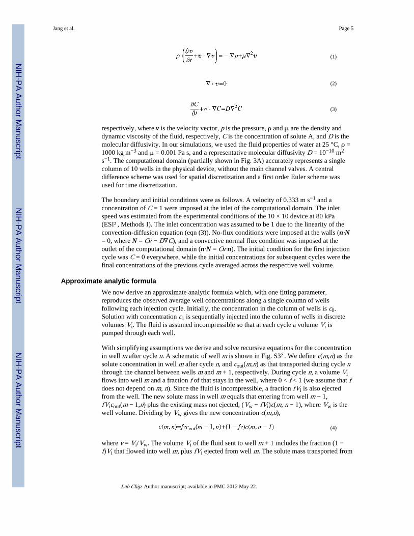
respectively, where v is the velocity vector, p is the pressure, ρ and μ are the density anddynamic viscosity of the fluid, respectively, C is the concentration of solute A, and D is themolecular diffusivity. In our simulations, we used the fluid properties of water at 25 °C, ρ =1000 kg m−3 and μ = 0.001 Pa s, and a representative molecular diffusivity D = 10−10 m2

s−1. The computational domain (partially shown in Fig. 3A) accurately represents a singlecolumn of 10 wells in the physical device, without the main channel valves. A centraldifference scheme was used for spatial discretization and a first order Euler scheme wasused for time discretization.

The boundary and initial conditions were as follows. A velocity of 0.333 m s−1 and aconcentration of C = 1 were imposed at the inlet of the computational domain. The inletspeed was estimated from the experimental conditions of the 10 × 10 device at 80 kPa(ESI†, Methods I). The inlet concentration was assumed to be 1 due to the linearity of theconvection-diffusion equation (eqn (3)). No-flux conditions were imposed at the walls (n·N= 0, where N = Cv − D∇C), and a convective normal flux condition was imposed at theoutlet of the computational domain (n·N = Cv·n). The initial condition for the first injectioncycle was C = 0 everywhere, while the initial concentrations for subsequent cycles were thefinal concentrations of the previous cycle averaged across the respective well volume.

Approximate analytic formulaWe now derive an approximate analytic formula which, with one fitting parameter,reproduces the observed average well concentrations along a single column of wellsfollowing each injection cycle. Initially, the concentration in the column of wells is c0.Solution with concentration c1 is sequentially injected into the column of wells in discretevolumes Vi. The fluid is assumed incompressible so that at each cycle a volume Vi ispumped through each well.

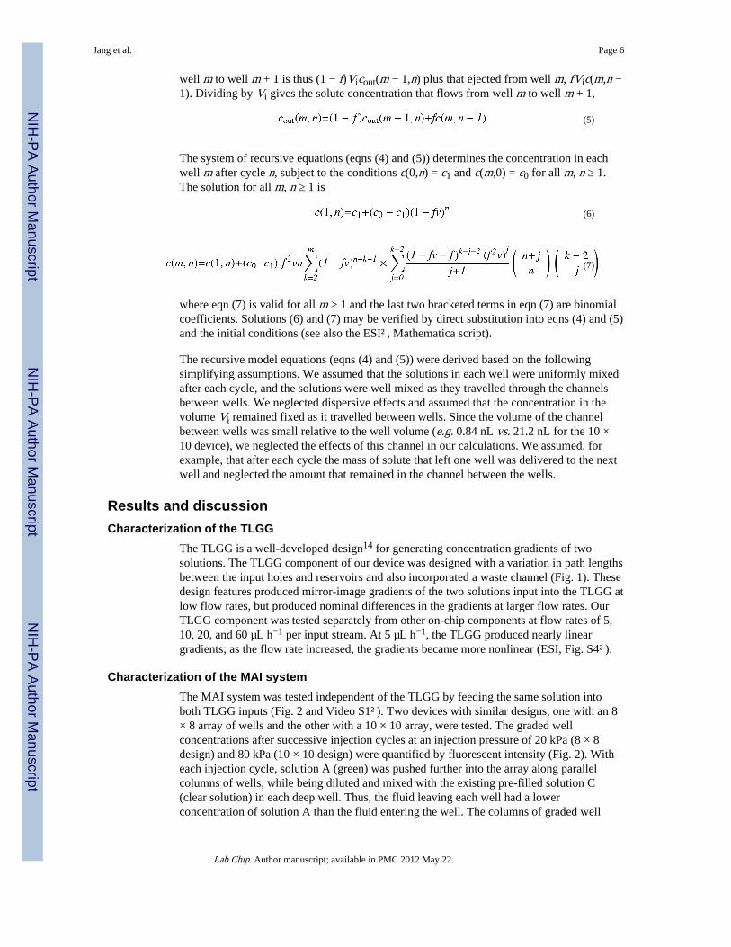
With simplifying assumptions we derive and solve recursive equations for the concentrationin well m after cycle n. A schematic of well m is shown in Fig. S3†. We define c(m,n) as thesolute concentration in well m after cycle n, and cout(m,n) as that transported during cycle nthrough the channel between wells m and m + 1, respectively. During cycle n, a volume Viflows into well m and a fraction f of that stays in the well, where 0 < f < 1 (we assume that fdoes not depend on m, n). Since the fluid is incompressible, a fraction fVi is also ejectedfrom the well. The new solute mass in well m equals that entering from well m − 1,fVicout(m − 1,n) plus the existing mass not ejected, (Vw − fVi)c(m, n − 1), where Vw is thewell volume. Dividing by Vw gives the new concentration c(m,n),

(4)

where v = Vi/Vw. The volume Vi of the fluid sent to well m + 1 includes the fraction (1 −f)Vi that flowed into well m, plus fVi ejected from well m. The solute mass transported from

Jang et al.


NIH


NIH


NIH


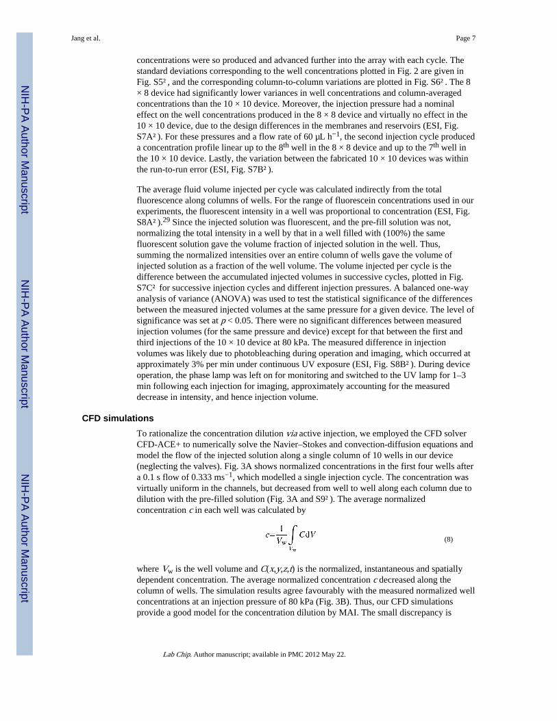
well m to well m + 1 is thus (1 − f)Vicout(m − 1,n) plus that ejected from well m, fVic(m,n −1). Dividing by Vi gives the solute concentration that flows from well m to well m + 1,

(5)

The system of recursive equations (eqns (4) and (5)) determines the concentration in eachwell m after cycle n, subject to the conditions c(0,n) = c1 and c(m,0) = c0 for all m, n ≥ 1.The solution for all m, n ≥ 1 is

(6)

(7)

where eqn (7) is valid for all m > 1 and the last two bracketed terms in eqn (7) are binomialcoefficients. Solutions (6) and (7) may be verified by direct substitution into eqns (4) and (5)and the initial conditions (see also the ESI†, Mathematica script).

The recursive model equations (eqns (4) and (5)) were derived based on the followingsimplifying assumptions. We assumed that the solutions in each well were uniformly mixedafter each cycle, and the solutions were well mixed as they travelled through the channelsbetween wells. We neglected dispersive effects and assumed that the concentration in thevolume Vi remained fixed as it travelled between wells. Since the volume of the channelbetween wells was small relative to the well volume (e.g. 0.84 nL vs. 21.2 nL for the 10 ×10 device), we neglected the effects of this channel in our calculations. We assumed, forexample, that after each cycle the mass of solute that left one well was delivered to the nextwell and neglected the amount that remained in the channel between the wells.

Results and discussionCharacterization of the TLGG

The TLGG is a well-developed design14 for generating concentration gradients of twosolutions. The TLGG component of our device was designed with a variation in path lengthsbetween the input holes and reservoirs and also incorporated a waste channel (Fig. 1). Thesedesign features produced mirror-image gradients of the two solutions input into the TLGG atlow flow rates, but produced nominal differences in the gradients at larger flow rates. OurTLGG component was tested separately from other on-chip components at flow rates of 5,10, 20, and 60 µL h−1 per input stream. At 5 µL h−1, the TLGG produced nearly lineargradients; as the flow rate increased, the gradients became more nonlinear (ESI, Fig. S4†).

Characterization of the MAI systemThe MAI system was tested independent of the TLGG by feeding the same solution intoboth TLGG inputs (Fig. 2 and Video S1†). Two devices with similar designs, one with an 8× 8 array of wells and the other with a 10 × 10 array, were tested. The graded wellconcentrations after successive injection cycles at an injection pressure of 20 kPa (8 × 8design) and 80 kPa (10 × 10 design) were quantified by fluorescent intensity (Fig. 2). Witheach injection cycle, solution A (green) was pushed further into the array along parallelcolumns of wells, while being diluted and mixed with the existing pre-filled solution C(clear solution) in each deep well. Thus, the fluid leaving each well had a lowerconcentration of solution A than the fluid entering the well. The columns of graded well

Jang et al.


NIH


NIH


NIH


concentrations were so produced and advanced further into the array with each cycle. Thestandard deviations corresponding to the well concentrations plotted in Fig. 2 are given inFig. S5†, and the corresponding column-to-column variations are plotted in Fig. S6†. The 8× 8 device had significantly lower variances in well concentrations and column-averagedconcentrations than the 10 × 10 device. Moreover, the injection pressure had a nominaleffect on the well concentrations produced in the 8 × 8 device and virtually no effect in the10 × 10 device, due to the design differences in the membranes and reservoirs (ESI, Fig.S7A†). For these pressures and a flow rate of 60 µL h−1, the second injection cycle produceda concentration profile linear up to the 8th well in the 8 × 8 device and up to the 7th well inthe 10 × 10 device. Lastly, the variation between the fabricated 10 × 10 devices was withinthe run-to-run error (ESI, Fig. S7B†).

The average fluid volume injected per cycle was calculated indirectly from the totalfluorescence along columns of wells. For the range of fluorescein concentrations used in ourexperiments, the fluorescent intensity in a well was proportional to concentration (ESI, Fig.S8A†).29 Since the injected solution was fluorescent, and the pre-fill solution was not,normalizing the total intensity in a well by that in a well filled with (100%) the samefluorescent solution gave the volume fraction of injected solution in the well. Thus,summing the normalized intensities over an entire column of wells gave the volume ofinjected solution as a fraction of the well volume. The volume injected per cycle is thedifference between the accumulated injected volumes in successive cycles, plotted in Fig.S7C† for successive injection cycles and different injection pressures. A balanced one-wayanalysis of variance (ANOVA) was used to test the statistical significance of the differencesbetween the measured injected volumes at the same pressure for a given device. The level ofsignificance was set at p < 0.05. There were no significant differences between measuredinjection volumes (for the same pressure and device) except for that between the first andthird injections of the 10 × 10 device at 80 kPa. The measured difference in injectionvolumes was likely due to photobleaching during operation and imaging, which occurred atapproximately 3% per min under continuous UV exposure (ESI, Fig. S8B†). During deviceoperation, the phase lamp was left on for monitoring and switched to the UV lamp for 1–3min following each injection for imaging, approximately accounting for the measureddecrease in intensity, and hence injection volume.

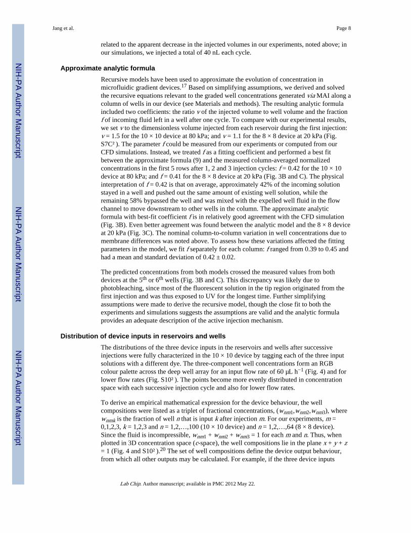
CFD simulationsTo rationalize the concentration dilution via active injection, we employed the CFD solverCFD-ACE+ to numerically solve the Navier–Stokes and convection-diffusion equations andmodel the flow of the injected solution along a single column of 10 wells in our device(neglecting the valves). Fig. 3A shows normalized concentrations in the first four wells aftera 0.1 s flow of 0.333 ms−1, which modelled a single injection cycle. The concentration wasvirtually uniform in the channels, but decreased from well to well along each column due todilution with the pre-filled solution (Fig. 3A and S9†). The average normalizedconcentration c in each well was calculated by

(8)

where Vw is the well volume and C(x,y,z,t) is the normalized, instantaneous and spatiallydependent concentration. The average normalized concentration c decreased along thecolumn of wells. The simulation results agree favourably with the measured normalized wellconcentrations at an injection pressure of 80 kPa (Fig. 3B). Thus, our CFD simulationsprovide a good model for the concentration dilution by MAI. The small discrepancy is

Jang et al.


NIH


NIH


NIH


related to the apparent decrease in the injected volumes in our experiments, noted above; inour simulations, we injected a total of 40 nL each cycle.

Approximate analytic formulaRecursive models have been used to approximate the evolution of concentration inmicrofluidic gradient devices.17 Based on simplifying assumptions, we derived and solvedthe recursive equations relevant to the graded well concentrations generated via MAI along acolumn of wells in our device (see Materials and methods). The resulting analytic formulaincluded two coefficients: the ratio v of the injected volume to well volume and the fractionf of incoming fluid left in a well after one cycle. To compare with our experimental results,we set v to the dimensionless volume injected from each reservoir during the first injection:v = 1.5 for the 10 × 10 device at 80 kPa; and v = 1.1 for the 8 × 8 device at 20 kPa (Fig.S7C†). The parameter f could be measured from our experiments or computed from ourCFD simulations. Instead, we treated f as a fitting coefficient and performed a best fitbetween the approximate formula (9) and the measured column-averaged normalizedconcentrations in the first 5 rows after 1, 2 and 3 injection cycles: f = 0.42 for the 10 × 10device at 80 kPa; and f = 0.41 for the 8 × 8 device at 20 kPa (Fig. 3B and C). The physicalinterpretation of f = 0.42 is that on average, approximately 42% of the incoming solutionstayed in a well and pushed out the same amount of existing well solution, while theremaining 58% bypassed the well and was mixed with the expelled well fluid in the flowchannel to move downstream to other wells in the column. The approximate analyticformula with best-fit coefficient f is in relatively good agreement with the CFD simulation(Fig. 3B). Even better agreement was found between the analytic model and the 8 × 8 deviceat 20 kPa (Fig. 3C). The nominal column-to-column variation in well concentrations due tomembrane differences was noted above. To assess how these variations affected the fittingparameters in the model, we fit f separately for each column: f ranged from 0.39 to 0.45 andhad a mean and standard deviation of 0.42 ± 0.02.

The predicted concentrations from both models crossed the measured values from bothdevices at the 5th or 6th wells (Fig. 3B and C). This discrepancy was likely due tophotobleaching, since most of the fluorescent solution in the tip region originated from thefirst injection and was thus exposed to UV for the longest time. Further simplifyingassumptions were made to derive the recursive model, though the close fit to both theexperiments and simulations suggests the assumptions are valid and the analytic formulaprovides an adequate description of the active injection mechanism.

Distribution of device inputs in reservoirs and wellsThe distributions of the three device inputs in the reservoirs and wells after successiveinjections were fully characterized in the 10 × 10 device by tagging each of the three inputsolutions with a different dye. The three-component well concentrations form an RGBcolour palette across the deep well array for an input flow rate of 60 µL h−1 (Fig. 4) and forlower flow rates (Fig. S10†). The points become more evenly distributed in concentrationspace with each successive injection cycle and also for lower flow rates.

To derive an empirical mathematical expression for the device behaviour, the wellcompositions were listed as a triplet of fractional concentrations, (wnm1,wnm2,wnm3), wherewnmk is the fraction of well n that is input k after injection m. For our experiments, m =0,1,2,3, k = 1,2,3 and n = 1,2,…,100 (10 × 10 device) and n = 1,2,…,64 (8 × 8 device).Since the fluid is incompressible, wnm1 + wnm2 + wnm3 = 1 for each m and n. Thus, whenplotted in 3D concentration space (c-space), the well compositions lie in the plane x + y + z= 1 (Fig. 4 and S10†).20 The set of well compositions define the device output behaviour,from which all other outputs may be calculated. For example, if the three device inputs

Jang et al.


NIH


NIH


NIH


contained the concentrations c1, c2, and c3 of a certain solution A, the resultingconcentration of A in well n after injection m would be the weighted average

(9)

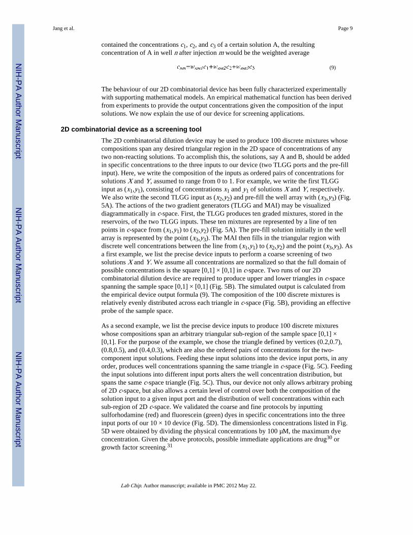
The behaviour of our 2D combinatorial device has been fully characterized experimentallywith supporting mathematical models. An empirical mathematical function has been derivedfrom experiments to provide the output concentrations given the composition of the inputsolutions. We now explain the use of our device for screening applications.

2D combinatorial device as a screening toolThe 2D combinatorial dilution device may be used to produce 100 discrete mixtures whosecompositions span any desired triangular region in the 2D space of concentrations of anytwo non-reacting solutions. To accomplish this, the solutions, say A and B, should be addedin specific concentrations to the three inputs to our device (two TLGG ports and the pre-fillinput). Here, we write the composition of the inputs as ordered pairs of concentrations forsolutions X and Y, assumed to range from 0 to 1. For example, we write the first TLGGinput as (x1,y1), consisting of concentrations x1 and y1 of solutions X and Y, respectively.We also write the second TLGG input as (x2,y2) and pre-fill the well array with (x3,y3) (Fig.5A). The actions of the two gradient generators (TLGG and MAI) may be visualizeddiagrammatically in c-space. First, the TLGG produces ten graded mixtures, stored in thereservoirs, of the two TLGG inputs. These ten mixtures are represented by a line of tenpoints in c-space from (x1,y1) to (x2,y2) (Fig. 5A). The pre-fill solution initially in the wellarray is represented by the point (x3,y3). The MAI then fills in the triangular region withdiscrete well concentrations between the line from (x1,y1) to (x2,y2) and the point (x3,y3). Asa first example, we list the precise device inputs to perform a coarse screening of twosolutions X and Y. We assume all concentrations are normalized so that the full domain ofpossible concentrations is the square [0,1] × [0,1] in c-space. Two runs of our 2Dcombinatorial dilution device are required to produce upper and lower triangles in c-spacespanning the sample space [0,1] × [0,1] (Fig. 5B). The simulated output is calculated fromthe empirical device output formula (9). The composition of the 100 discrete mixtures isrelatively evenly distributed across each triangle in c-space (Fig. 5B), providing an effectiveprobe of the sample space.

As a second example, we list the precise device inputs to produce 100 discrete mixtureswhose compositions span an arbitrary triangular sub-region of the sample space [0,1] ×[0,1]. For the purpose of the example, we chose the triangle defined by vertices (0.2,0.7),(0.8,0.5), and (0.4,0.3), which are also the ordered pairs of concentrations for the two-component input solutions. Feeding these input solutions into the device input ports, in anyorder, produces well concentrations spanning the same triangle in c-space (Fig. 5C). Feedingthe input solutions into different input ports alters the well concentration distribution, butspans the same c-space triangle (Fig. 5C). Thus, our device not only allows arbitrary probingof 2D c-space, but also allows a certain level of control over both the composition of thesolution input to a given input port and the distribution of well concentrations within eachsub-region of 2D c-space. We validated the coarse and fine protocols by inputtingsulforhodamine (red) and fluorescein (green) dyes in specific concentrations into the threeinput ports of our 10 × 10 device (Fig. 5D). The dimensionless concentrations listed in Fig.5D were obtained by dividing the physical concentrations by 100 µM, the maximum dyeconcentration. Given the above protocols, possible immediate applications are drug30 orgrowth factor screening.31

Jang et al.


NIH


NIH


NIH


Additional remarksOur device has several advantages over existing approaches. (1) The MAI mechanism cangenerate a graded sequence of well concentrations in seconds with one injection cycle. Theunderlying convection-based mixing is orders of magnitude faster than diffusion-limitedmixing.11,18,19 The MAI reduces the overall preparation time of the 2D gradient, importantfor time-sensitive applications such as cytotoxicity studies. (2) The MAI mechanism may bereadily combined with gradient generators, such as the TLGG in the present work, to create2D combinatorial mixtures. In fact, replacing the TLGG in our device with a second MAIsystem could dramatically reduce the overall device operation time. (3) The sequence ofwell concentrations can be tuned by adjusting the flow rate and the number of injectioncycles. (4) The MAI mechanism is integrated with the deep well array, making the devicecompact and allowing the combinatorial mixtures to be isolated in the deep wells. As in asimilar device, cells would be loaded with the pre-fill solution and allowed to settle to thebase of the wells, where they would be protected from the flow shear induced by activeinjection.32 (5) Finally, the MAI mechanism dispenses into and traps in each well a finiteliquid volume, enabling discrete increments of soluble factors to be tested on a sample.

Further improvements could be made to our 2D combinatorial dilution device. (1) Thecolumn-to-column and device-to-device variation could be improved by increasing thedesign and fabrication uniformity of the thin membranes inside the MAI injectors. Theassembly of the device currently requires careful alignment; improved designs couldsimplify assembly. (2) Due to the relatively small well volumes (20 nL), maintainingconstant conditions in a well for prolonged durations could require additional injectioncycles to replace liquid absorbed by the PDMS or, in the case of cell-based applications,soluble factors consumed by cells. However, in isolated wells of similar volumes (~20 nL),50–100 cells per well remained at least 88% viable when incubated for at least 24 h withoutmedia replacement.6,32 For longer durations, a multi-step experimental protocol involving asolution replacement step and a gradient re-generation step could overcome this issue. (3)The MAI establishes a concentration profile via rapid injection (>0.3 m s−1) of solution fromchannels to deep wells. The complex fluidic behaviour may hinder design modifications forobtaining arbitrary profiles from the MAI mechanism. Despite the flow complexity, wederived simple mathematical expressions that adequately described the resulting averageconcentrations; similar approaches could be used for modified designs. (4) Creating particlegradients with the injection mechanism would be problematic due to clogging, whilegradients of larger molecules such as polymer solutions would require more time fordiffusion to mix solutions in each well between injection cycles. Other mechanisms exist forthese purposes.5,18 (5) Finally, since the active injection mechanism uses the wells asdilution mechanisms, the contents of the wells during pre-fill and intermediate injectionsgenerally differ from the final combinatorial mixtures. Thus, for applications involving cells,which would generally be loaded with or before the pre-fill solution, the cells would beexposed to intermediate well mixtures during device operation. Related side-effects could bereduced by expediting the formation of the combinatorial well contents. Moreover, feedingthree input solutions into the input ports in any order yields well concentrations spanning thesame triangle in c-space (Fig. 5C). Thus, for a particular screening, the user is given someflexibility as to the input composition and could, for example, load the least reactive orharmful components/concentrations into the pre-fill solution.

ConclusionsIn this paper we presented a new integrated microfluidic device incorporating two gradientgenerators, the TLGG and MAI, that, in concert, produced graded combinations of threeinput solutions across 8 × 8 or 10 × 10 arrays of deep wells. The compositions of thesolutions stored in the arrays were evenly distributed across planar concentration surfaces,

Jang et al.


NIH


NIH


NIH


rendering the device ideal for combinatorial and dosimetry studies. In particular, preciseprotocols were given to use the device as a screening platform to investigate the synergisticeffects of pairs of factors on biological entities. The functionality of the active injectionmechanism was adequately modelled by both computational simulations and an approximateanalytic formula, providing ample design criteria for future device use and modification.The device design is naturally scalable to larger arrays, while other combinatorialconcentrations may be obtained by using other existing gradient generators.

Supplementary MaterialRefer to Web version on PubMed Central for supplementary material.

AcknowledgmentsThis paper was supported by the National Institutes of Health (EB008392; HL092836; DE019024; EB012597;DE021468), the National Science Foundation (DMR0847287), the Institute for Soldier Nanotechnology, the Officeof Naval Research, and the US Army Corps of Engineers. Y. H. Jang was partially supported by the NationalResearch Foundation of Korea (Grant NRF-2009-352-D00107).

References1. Rasmussen BF, Stock AM, Ringe D, Petsko GA. Nature. 1992; 357:423–424. [PubMed: 1463484]

2. Masscheleyn PH, Delaune RD, Patrick WH. Environ. Sci. Technol. 1991; 25:1414–1419.

3. Flaim CJ, Chien S, Bhatia SN. Nat. Methods. 2005; 2:119–125. [PubMed: 15782209] Tavana H,Jovic A, Mosadegh B, Lee QY, Liu X, Luker KE, Luker GD, Weiss SJ, Takayama S. Nat. Mater.2009; 8:736–741. [PubMed: 19684584] Anderson DG, Levenberg S, Langer R. Nat. Biotechnol.2004; 22:863–866. [PubMed: 15195101]

4. Khademhosseini A, Langer R, Borenstein J, Vacanti J. Proc. Natl. Acad. Sci. U. S. A. 2006;103:2480–2487. [PubMed: 16477028]

5. He J, Du Y, Villa-Uribe JL, Hwang C, Li D, Khademhosseini A. Adv. Funct. Mater. 2010; 20:131–137. [PubMed: 20216924]

6. Wu J, Wheeldon I, Guo Y, Lu T, Du Y, Wang B, He J, Hu Y, Khademhosseini A. Biomaterials.2011; 32:841–848. [PubMed: 20965560]

7. Keenan TM, Folch A. Lab Chip. 2008; 8:34–57. [PubMed: 18094760]

8. Kim L, Vahey MD, Lee HY, Voldman J. Lab Chip. 2006; 6:394–406. [PubMed: 16511623]

9. Cappiello A, Famiglini G, Fiorucci C, Mangani F, Palma P, Siviero A. Anal. Chem. 2003; 75:1173–1179. [PubMed: 12641238]

10. Hung PJ, Lee PJ, Sabounchi P, Aghdam N, Lin R, Lee LP. Lab Chip. 2005; 5:44–48. [PubMed:15616739] Hung PJ, Lee PJ, Sabounchi P, Lin R, Lee LP. Biotechnol. Bioeng. 2005; 89:1–8.[PubMed: 15580587] Selimović š, Sim WY, Kim SB, Jang Y-H, Lee WG, Khabiry M, Bae H,Jambovane S, Hong JW, Khademhosseini A. Anal. Chem. 2011; 83:2020–2028. [PubMed:21344866]

11. Mosadegh B, Agarwal M, Tavana H, Bersano-Begey T, Torisawa Y-s, Morell M, Wyatt MJ,O’Shea KS, Barald KF, Takayama S. Lab Chip. 2010; 10:2959–2964. [PubMed: 20835429]

12. Hancock MJ, He J, Mano JF, Khademhosseini A. Small. 2011; 7:892–901. [PubMed: 21374805]

13. Sun K, Wang Z, Jiang X. Lab Chip. 2008; 8:1536–1543. [PubMed: 18818810]

14. Jeon NL, Dertinger SKW, Chiu DT, Choi IS, Stroock AD, Whitesides GM. Langmuir. 2000;16:8311–8316.

15. Dertinger SKW, Chiu DT, Jeon NL, Whitesides GM. Anal. Chem. 2001; 73:1240–1246.Jeon NL,Baskaran H, Dertinger SKW, Whitesides GM, Van De Water L, Toner M. Nat. Biotechnol. 2002;20:826–830. [PubMed: 12091913] Cimetta E, Cannizzaro C, James R, Biechele T, Moon R,Elvassore N, Vunjak-Novakovic G. Lab Chip. 2010; 10:3277–3283. [PubMed: 20936235]

16. Lee K, Kim C, Ahn B, Panchapakesan R, Full AR, Nordee L, Kang JY, Oh KW. Lab Chip. 2009;9:709–717. [PubMed: 19224022] Hattori K, Sugiura S, Kanamori T. Lab Chip. 2009; 9:1763–

Jang et al.


NIH


NIH


NIH


1772. [PubMed: 19495461] Sugiura S, Hattori K, Kanamori T. Anal. Chem. 2010; 82:8278–8282.[PubMed: 20822164] Saadi W, Rhee SW, Lin F, Vahidi B, Chung BG, Jeon NL. Biomed.Microdevices. 2007; 9:627–635. [PubMed: 17530414]

17. Irimia D, Geba DA, Toner M. Anal. Chem. 2006; 78:3472–3477. [PubMed: 16689552]

18. Du Y, Hancock MJ, He J, Villa-Uribe JL, Wang B, Cropek DM, Khademhosseini A. Biomaterials.2010; 31:2686–2694. [PubMed: 20035990]

19. Du Y, Shim J, Vidula M, Hancock MJ, Lo E, Chung BG, Borenstein JT, Khabiry M, Cropek DM,Khademhosseini A. Lab Chip. 2009; 9:761–767. [PubMed: 19255657]

20. Lee K, Kim C, Kim Y, Ahn B, Bang J, Kim J, Panchapakesan R, Yoon Y-K, Kang J, Oh K.Microfluid. Nanofluid. 2011; 11:75–86.

21. Atencia J, Morrow J, Locascio LE. Lab Chip. 2009; 9:2707–2714. [PubMed: 19704987] ChungBG, Lin F, Jeon NL. Lab Chip. 2006; 6:764–768. [PubMed: 16738728]

22. Cooksey GA, Sip CG, Folch A. Lab Chip. 2009; 9:417–426. [PubMed: 19156291]

23. Neils C, Tyree Z, Finlayson B, Folch A. Lab Chip. 2004; 4:342–350. [PubMed: 15269802]

24. Lee K, Kim C, Jung G, Kim TS, Kang JY, Oh KW. Microfluid. Nanofluid. 2010; 8:677–685.Titmarsh D, Cooper-White J. Biotechnol. Bioeng. 2009; 104:1240–1244. [PubMed:19685525]

25. Liu MC, Ho D, Tai YC. Sens. Actuators, B. 2008; 129:826–833.

26. Hansen CL, Sommer MOA, Quake SR. Proc. Natl. Acad. Sci. U. S. A. 2004; 101:14431–14436.[PubMed: 15452343]

27. Shankar PN. J. Fluid Mech. 1997; 342:97–118.Shankar PN, Deshpande MD. Annu. Rev. FluidMech. 2000; 32:93–136.

28. Holden MA, Kumar S, Castellana ET, Beskok A, Cremer PS. Sens. Actuators, B. 2003; 92:199–207.

29. Lin F, Saadi W, Rhee SW, Wang SJ, Mittal S, Jeon NL. Lab Chip. 2004; 4:164–167. [PubMed:15159771]

30. Ye N, Qin J, Shi W, Liu X, Lin B. Lab Chip. 2007; 7:1696–1704. [PubMed: 18030389]

31. Lee LH, Peerani R, Ungrin M, Joshi C, Kumacheva E, Zandstra P. Stem Cell Res. 2009; 2:155–162. [PubMed: 19383420]

32. Jang Y-H, Kwon CH, Kim SB, Selimović š, Sim WY, Bae H, Khademhosseini A. Biotechnol. J.2011; 6:156–164. [PubMed: 21298801]

Jang et al.


NIH


NIH


NIH


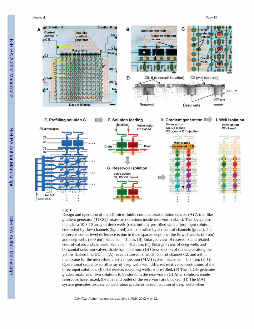
Fig. 1.Design and operation of the 2D microfluidic combinatorial dilution device. (A) A tree-likegradient generator (TLGG) mixes two solutions inside reservoirs (black). The device alsoincludes a 10 × 10 array of deep wells (red), initially pre-filled with a third input solution,connected by flow channels (light red) and controlled by six control channels (green). Theobserved colour level difference is due to the disparate depths of the flow channels (20 µm)and deep wells (300 µm). Scale bar = 1 mm. (B) Enlarged view of reservoirs and relatedcontrol valves and channels. Scale bar = 0.3 mm. (C) Enlarged view of deep wells andhorizontal selection valves. Scale bar = 0.3 mm. (D) Cross-section of the device along theyellow dashed line DD′ in (A) reveals reservoirs, wells, control channel C2, and a thinmembrane for the microfluidic active injection (MAI) system. Scale bar = 0.3 mm. (E–G)Operational sequence to fill array of deep wells with different relative concentrations of thethree input solutions. (E) The device, including wells, is pre-filled. (F) The TLGG generatesgraded mixtures of two solutions to be stored in the reservoirs. (G) After solutions insidereservoirs have mixed, the inlet and outlet of the reservoirs are blocked. (H) The MAIsystem generates discrete concentration gradients in each column of deep wells when

Jang et al.


NIH


NIH


NIH


positive pressure is applied on the C1 control channel for 5 seconds. (I) All valves are closedto isolate and maintain the mixture in each well, stabilizing the 2D combinatorial mixtureacross the array.

Jang et al.


NIH


NIH


NIH


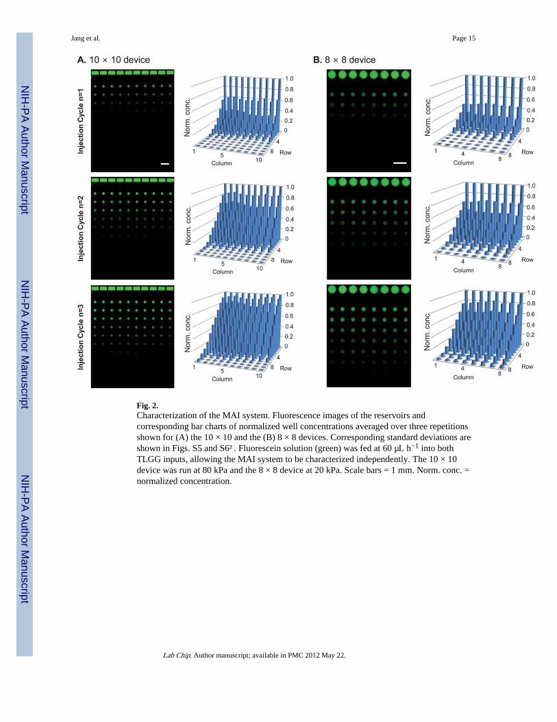
Fig. 2.Characterization of the MAI system. Fluorescence images of the reservoirs andcorresponding bar charts of normalized well concentrations averaged over three repetitionsshown for (A) the 10 × 10 and the (B) 8 × 8 devices. Corresponding standard deviations areshown in Figs. S5 and S6†. Fluorescein solution (green) was fed at 60 µL h−1 into bothTLGG inputs, allowing the MAI system to be characterized independently. The 10 × 10device was run at 80 kPa and the 8 × 8 device at 20 kPa. Scale bars = 1 mm. Norm. conc. =normalized concentration.

Jang et al.


NIH


NIH


NIH


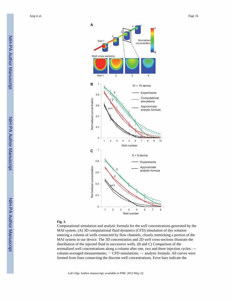
Fig. 3.Computational simulation and analytic formula for the well concentrations generated by theMAI system. (A) 3D computational fluid dynamics (CFD) simulation of dye solutionentering a column of wells connected by flow channels, closely mimicking a portion of theMAI system in our device. The 3D concentration and 2D well cross-sections illustrate thedistribution of the injected fluid in successive wells. (B and C) Comparison of thenormalized well concentrations along a column after one, two and three injection cycles: —column-averaged measurements; ⋯ CFD simulations; --- analytic formula. All curves wereformed from lines connecting the discrete well concentrations. Error bars indicate the

Jang et al.


NIH


NIH


NIH


standard deviation over three experimental runs of the same device. Results reported for the(B) 10 × 10 and (C) 8 × 8 designs.

Jang et al.


NIH


NIH


NIH


Fig. 4.Relative distribution of the three device inputs in the reservoirs and wells. Combined actionof the TLGG and MAI mechanisms filled the 10 × 10 well array with different fractions ofthe three input solutions. The three input solutions each contained a different fluorescentdye: fluorescein sodium salt (TLGG input 1, solution A, green); sulforhodamine 101 (TLGGinput 2, solution B, red); and calcein blue (pre-fill input, solution C). Before injection, allwells were pre-filled with solution C while the reservoirs contained the TLGG-generatedAB mixtures. Subsequent injections propelled the AB mixtures from the reservoirs throughparallel columns of wells where they were sequentially diluted. The input flow rate of theTLGG was 60 µL h−1 and reservoirs were stabilized for 10 min. (Top row) Fluorescenceimages of the reservoirs and wells indicate their relative compositions before injection andafter subsequent injection cycles. (Bottom row) Corresponding concentration space (c-space) plots of the fractional compositions of the reservoirs and wells. The points lie in theplane x + y + z = 1 since the fractions add to 1. Scale bar = 1 mm.

Jang et al.


NIH


NIH


NIH


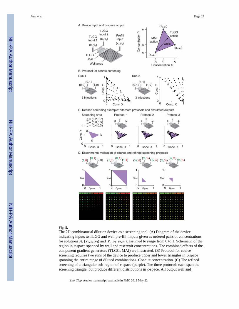
Fig. 5.The 2D combinatorial dilution device as a screening tool. (A) Diagram of the deviceindicating inputs to TLGG and well pre-fill. Inputs given as ordered pairs of concentrationsfor solutions X, (x1,x2,x3) and Y, (y1,y2,y3), assumed to range from 0 to 1. Schematic of theregion in c-space spanned by well and reservoir concentrations. The combined effects of thecomponent gradient generators (TLGG, MAI) are illustrated. (B) Protocol for coarsescreening requires two runs of the device to produce upper and lower triangles in c-spacespanning the entire range of diluted combinations. Conc. = concentration. (C) The refinedscreening of a triangular sub-region of c-space (purple). The three protocols each span thescreening triangle, but produce different distributions in c-space. All output well and

Jang et al.


NIH


NIH


NIH


reservoir concentrations were calculated from the output formula (9) derived fromexperimental data. (D) Experimental validation of the coarse and refined screeningprotocols. The device inputs are illustrated at the top, the triangular screening regions areshown below, followed by the resulting fluorescence images.

Jang et al.


NIH


NIH


NIH


An integrated microfluidic device for two-dimensional combinatorial dilution

Documents

Transcript of An integrated microfluidic device for two-dimensional combinatorial dilution