Noname manuscript No.(will be inserted by the editor)

From approximating to interpolatory non-stationarysubdivision schemes with the same reproduction properties

Costanza Conti · Luca Gemignani · Lucia

Romani

Received: date / Accepted: date

Abstract In this paper we describe a general, computationally feasible strategy to

deduce a family of interpolatory non-stationary subdivision schemes from a symmetric

non-stationary, non-interpolatory one satisfying quite mild assumptions. It is shown

that the interpolatory schemes are (mostly) capable of generating the same functional

space as the approximating one. Moreover, the interplay between structured matri-

ces and polynomials provides an effective tool for designing efficient numeric and/or

numeric-symbolic methods for their construction and analysis.

Keywords Subdivision schemes · Structured matrices · Polynomials

Mathematics Subject Classification (2000) MSC 65F05 · MSC 65D05

1 Introduction

This paper is the generalization of our recent work [2] to the non-stationary situation.

In fact, many important subdivision schemes are of non-stationary nature like those

able to reproduce conic sections, spirals or classical trigonometric curves which are

important analytical shapes in geometric modeling. In particular we discuss how it is

possible to move from a non-stationary approximating subdivision scheme to a non-

stationary interpolatory one.

C. ContiDipartimento di Energetica “Sergio Stecco”, Universita di Firenze,Via Lombroso 6/17, 50134 Firenze, ItalyE-mail: costanza.conti@unifi.it

L. GemignaniDipartimento di Matematica, Universita di Pisa,Largo Bruno Pontecorvo 5, 56127 Pisa, ItalyE-mail: gemignan@dm.unipi.it

L. RomaniDipartimento di Matematica e Applicazioni, Universita di Milano-Bicocca,Via R. Cozzi 53, 20125 Milano, ItalyE-mail: lucia.romani@unimib.it

2

Interpolatory subdivision schemes are efficient iterative procedures for the gene-

ration of interpolatory curves: Starting with the set of points to be interpolated, at

each recursion step a new point is inserted in between any two given points so that

the limit curve, whenever exists, not only interpolates the initial set of points but also

all the points generated through the process. Interpolatory subdivision schemes play a

crucial role in CAGD as well as in wavelets construction (see for example [5] and [8],

respectively). Indeed, from a positive symmetric interpolatory symbol, via its spectral

factorization, we can construct an orthogonal refinable function that is the building

block of orthonormal wavelets.

In this paper we provide a general strategy to deduce a family of interpolatory non-

stationary subdivision schemes from a symmetric non-stationary, non-interpolatory one

satisfying quite mild assumptions. In most cases the resulting interpolatory schemes

have the remarkable property of generating the same functional space as the approxi-

mating one. The approximating symbols we start with, say {ak(z), k ≥ 0}, are required

to be symmetric polynomials such that ak(z), ak(−z) are relatively prime for any

k ≥ 0. Under this assumption we show that a family of interpolatory masks associated

with the symbol ak(z) can be generated by solving a family of Bezout-like polynomial

equations or, equivalently, by inverting a certain Hurwitz matrix constructed from the

coefficients of ak(z).

From a computational viewpoint, the interplay between the polynomial and the

structured matrix formulation turns out to be an effective tool for the construction

and the analysis of the interpolatory schemes. If ak(z) is a Hurwitz polynomial, then

the associated Hurwitz matrix is totally positive and, therefore, can be factorized and

inverted stably by using techniques based on Neville’s elimination [7]. A root-based

polynomial equation solver leads to an efficient strategy for the computation of the

coefficients of the corresponding interpolatory symbols in several important cases where

the zeros of ak(z) are known a-priori. Furthermore, a specific mixed strategy based on

polynomial and matrix computations can be especially efficient in situations where the

polynomial ak(z) admits a “short” representation in some Bernstein-type polynomial

basis. All these approaches together allow us to efficiently address the case of B-splines

and their “shifted” affine combinations as well as the case of exponential reproducing

splines (ERS).

The paper is organized as follows. In Section 2 the needed background on non-

stationary subdivision schemes is given. In Section 3 we review and generalize to some

extent the basic strategy proposed in [2] for the construction of an interpolatory sub-

division mask from a given approximating one. Effective computational procedures

for implementing this strategy are discussed in Section 4. These procedures are the

key ingredients of our algorithm, named Appint, to move from a non-stationary ap-

proximating subdivision scheme to a family of non-stationary interpolatory ones. The

algorithm is sketched in Section 5 by showing the reproduction property of the gen-

erated schemes. Then, Section 6 discusses the application of the Appint Algorithm to

(non-stationary) B-spline symbols and their “shifted” affine combinations, whereas in

Section 7 the application of the algorithm to several instances of non-stationary ap-

proximating exponential reproducing subdivision schemes is considered. Finally, the

conclusion and further work are drawn in Section 8.

3

2 Background

Any (non-stationary) subdivision scheme is defined by an infinite sequence of refine-

ment masks {ak, k ≥ 0}. We assume that any sequence ak :=(ak

i , i ∈ Z)

is of real

numbers and has finite support for all k ≥ 0 i.e. aki = 0 for i 6∈ [−n(k), n(k)] for

suitable n(k) ≥ 0. The k-level subdivision operator associated with the k-level mask ak

isSak : `(Z) → `(Z) ,

(Sak q)i :=∑

j∈Zak

i−2j qj , i ∈ Z ,(2.1)

where `(Z) denotes the linear space of real sequences indexed by Z whose elements will

be denoted by boldface letter, q = (qi ∈ R, i ∈ Z).

The non-stationary subdivision scheme consists of the subsequent application of

Sa0 , · · · , Sak from a given starting sequence, say q, generating the scalar sequences

q0 := q , qk+1 := Sak qk for k ≥ 0.

A subdivision scheme is termed L∞-convergent if, for any q ∈ `∞(Z), the linear

subspace of bounded scalar sequences, there exists a continuous function fq (depending

on the starting sequence q) satisfying

limk→∞

∥∥∥fq( ·

2k

)− qk

∥∥∥∞ = 0

and fq 6= 0 for at least some initial data q. Here, the symbol fq( ·2k ) abbreviates the

scalar sequence{fq

(i

2k

)}i∈Z and ‖q‖∞ := supi∈Z | qi|.

The limit of the subdivision process when starting with q = δ := (δi,0 : i ∈ Z), where

δi,j is the Kronecker delta symbol, is called its basic limit function and is denoted by

φ.

Useful tools for the subdivision analysis are the symbols

ak(z) =∑

i∈Zak

i zi, k ≥ 0, z ∈ C \ {0}

and the corresponding sub–symbols

akeven(z) =

∑

i∈Zak2i zi, ak

odd(z) =∑

i∈Zak2i+1 zi, z ∈ C \ {0},

with

akeven(z2) + z · ak

odd(z2) = ak(z),

associated to the masks {ak, k ≥ 0}. Since the masks are always supposed to be finitely

supported, all symbols are Laurent polynomials. We observe that the conditions

ak(1) = 2, ak(−1) = 0, k ≥ 0 (2.2)

ensure reproduction of constant sequences, a minimal request for a scheme to be ef-

fective. In the stationary case, where the masks {ak, k ≥ 0} are kept fixed over the

iterations, that is ak = a for all k ≥ 0, the conditions (2.2) become a necessary condi-

tion for convergence, i.e.

a(1) = 2, a(−1) = 0.

4

A well known class of stationary subdivision schemes is given by degree-n B-spline

subdivision schemes, whose symbol is

a(z) = an(z) =(1 + z)n+1

2n. (2.3)

The non-stationary counterpart of (2.3) is the symbol of the so-called L-spline

schemes [12], a large family of smoothing splines defined in terms of a linear diffe-

rential operator, that we recall in the next definition. Since they are able to gene-

rate exponential polynomials, they turn out to be of great interest in curve design

for reproducing important analytical shapes like conic sections, spirals and classical

trigonometric curves.

Definition 1 (Space of Exponential Polynomials) Let T ∈ Z+ and γ = (γ0, γ1, · · · , γT )

with γT 6= 0 a finite set of real or imaginary numbers and let Dn the n-th order diffe-

rentiation operator. The space of exponential polynomials VT,γ is the subspace

VT,γ := {f : R→ C, f ∈ CT (R) :

T∑

j=0

γjDj f = 0}. (2.4)

A characterization of the space VT,γ is provided by the following:

Lemma 1 [9,13] Let γ(z) =∑T

j=0 γjzj and denote by {θ`, τ`}`=1,··· ,N the set of zeros

with multiplicity of γ(z) satisfying

γ(h`)(θ`) = 0, h` = 0, · · · , τ` − 1, ` = 1, · · · , N.

It results

T =

N∑

`=1

τ`, VT,γ := Span{xh`eθ` x, h` = 0, · · · , τ` − 1, ` = 1, · · · , N}.

As proved in [13], any non-stationary subdivision scheme with a symbol of the form

akn(z) = 2

N∏

`=1

τ`−1∏

h`=0

eθ`

2k+1 z + 1

eθ`

2k+1 + 1, k ≥ 0 , (2.5)

generates limit functions belonging to the subclass of CT−2 degree-n L-splines (with

n = T − 1) whose pieces are exponentials of the space VT,γ . These functions are called

exponential reproducing splines (ERS). Notice that, when θ` = 0 for all ` = 1, ..., N ,

then akn(z) in (2.5) does not depend on k being the symbol of a degree-n B-spline given

in (2.3).

We conclude by recalling that a subdivision scheme is said to be interpolatory if the

refinement masks {ak, k ≥ 0} satisfy

ak2i = δi,0, k ≥ 0,

or equivalently

akeven(z) = 1 (2.6)

meaning that all points generated by the subdivision process at a given level k will

be kept in the next level k + 1. In the latter case, any basic limit function is cardinal

since it satisfies φ(i) = δi,0. We conclude by mentioning that from (2.6) it follows that

a mask ak is interpolatory if and only if all its symbols ak(z) satisfy the condition

ak(z) + ak(−z) = 2. (2.7)

5

3 From approximating to interpolatory subdivision schemes: The general

approach

In this section we review and generalize to some extent the strategy proposed by the

authors in [2] to construct a family of interpolatory subdivision symbols from a non-

interpolatory one ak(z) for k fixed, k ∈ Z, k ≥ 0. For the sake of notational simplicity

we omit the superscript k by denoting ak(z) = a(z) =∑

i∈Z aizi, z ∈ C \ {0}.

It is worth noting that in a matrix setting the linear operator Sa defined in

(2.1) and associated with a(z) is represented by a bi-infinite Toeplitz-like matrix

Sa = (ai−2j), i, j ∈ Z. Since a(z) is a Laurent polynomial, say a(z) =∑κ

j=−κ ajzj ,

max{|a−κ|, |aκ|} > 0, it follows that Sa is banded with bandwidth dκ2 e at most. Let

p(z) =∑h

j=−h pjzj , max{|p−h|, |ph|} > 0, be another Laurent polynomial and denote

by P the bi-infinite Toeplitz matrix associated with p(z), namely, P = (pi−j). Observe

that P is again banded with bandwidth h. For the product operator

S : = P · Sa = (si,j), i, j ∈ Z,

we have

si,j =

i+h∑

r=i−h

pi−r ar−2j =

h∑

`=−h

p` ai−2j−` = si+2,j+1, i, j ∈ Z.

This means that the product operator S is a bi-infinite Toeplitz-like matrix of the same

form as the subdivision operator Sa with entries si,j = si−2j , i, j ∈ Z. By setting

q(z) = a(z) · p(z) =

h+κ∑

j=−h−κ

qjzj , (qj = 0 if |j| > h + κ),

we find that

qj =

h∑

i=−h

pi aj−i, −(h + κ) ≤ j ≤ h + κ,

and, therefore,

qi−2j = si,j = si−2j , i, j ∈ Z.

There follows that the product operator S can be seen as the subdivision operator

associated with the Laurent polynomial q(z), i.e.,

S = Sq, q(z) = a(z) · p(z),

where a(z) is the symbol of Sa and p(z) can be suitably chosen in such a way to satisfy

the interpolation condition. By expressing q(z) in terms of its sub–symbols

q(z) = q even(z2) + z · q odd(z2) z ∈ C \ {0},

we find that

q(z) + q(−z) = 2 · q even(z2).

Then by imposing the interpolation condition (2.6), i.e., q even(z) = 1, we arrive at

the relation

a(z) · p(z) + a(−z)p(−z) = 2 (3.8)

6

which is a generalized Bezout equation providing necessary and sufficient conditions

for a Laurent polynomial p(z) to convert the subdivision operator associated with a(z)

into the interpolating subdivision operator generated by q(z) = a(z) · p(z).

Suitable coefficient-wise representations of p(z) are introduced to investigate con-

ditions under which the (generalized) Bezout equation is solvable as well as to develop

effective computational methods for its solution. In the sequel of this section the sought

polynomial p(z) is of the form

p(z) = p1(z) : = pκzκ + pκ+1zκ+1 + . . . + pκ+mzκ+m, (3.9)

or

p(z) = p2(z) : = z · p1(z), (3.10)

with 2κ = m + 1. For such given polynomials p(z) the product Laurent polynomial

q(z) = a(z) · p(z) can be expressed as

q(z) = a(z) · p1(z) =

2κ+m∑

`=0

q`z` =

2m+1∑

`=0

q`z`,

and

q(z) = a(z) · p2(z) =

2κ+m+1∑

`=1

q`z` =

2m+2∑

`=1

q`z`.

Therefore we can try to determine the m + 1 unknown coefficients of p(z) to satisfy

the following modified forms of (3.8)

a(z) · p1(z) + a(−z) · p1(−z) = 2z2s, 0 ≤ s ≤ m, (3.11)

and

a(z) · p2(z) + a(−z) · p2(−z) = 2z2s, 1 ≤ s ≤ m + 1, (3.12)

or, equivalently,

a(z) · p1(z)− a(−z) · p1(−z) = 2z2s−1, 1 ≤ s ≤ m + 1. (3.13)

Indeed, it is clear that a solution of (3.11) or (3.13) provides a solution of (3.8) obtained

by simply shifting the coefficient-wise representation of p(z).

In a matrix setting the solution of (3.11) and (3.13) reduces to solving a structured

linear system whose coefficient matrix is Sylvester-like. Let a0 = [a−κ, . . . , a0, . . . , aκ]T

∈ R2κ+1 denote the coefficient vector of the Laurent polynomial a(z). The associa-

ted extended coefficient vector a+ ∈ R2κ+m+1 is defined by aT0 =

[aT

0 , 0, . . . , 0].

Similarly let us introduce the extended coefficient vector a− ∈ R2κ+m+1 associated

with the polynomial a(−z). Moreover let Z = (zi,j) ∈ R2(m+1)×2(m+1) be the down-

shift matrix given by zi,j = δi−1,j , where δi,j is the Kronecker delta symbol. Set

R+ ∈ R2(m+1)×(m+1) the striped Toeplitz matrix

R+ =[a+|Za+| . . . |Zma+

],

and, similarly, define

R− =[a−|Za−| . . . |Zma−

].

7

The coefficient matrix of the linear system (3.11) and (3.13) is R = [R+|R−] ∈R2(m+1)×2(m+1). It is well known that R is invertible if and only if a(z) and a(−z)

are relatively prime polynomials.

A different, alternative reduction which is useful for the computation of p(z) is

the following. From the interpolation condition q even(z2) = z2s for a suitable s, we

obtain thatm∑

`=0

q2`z` = zs, 0 ≤ s ≤ m, (q(z) = a(z) · p1(z)), (3.14)

orm+1∑

`=1

q2`z` = zs, 1 ≤ s ≤ m + 1, (q(z) = a(z) · p2(z)). (3.15)

The equations (3.14) translate in a linear system whose coefficient matrixH1 ∈ R(m+1)×(m+1)

is of Hurwitz type, namely,

H1 =

a−κ 0 . . . . . . . . .

a−κ+2 a−κ+1 a−κ 0 . . .

a−κ+4 a−κ+3 a−κ+2 . . . . . ....

......

... . . ....

......

... . . .

a−κ+2m a−κ+2m−1 a−κ+2m−2 . . . . . .

.

Similarly, the equations (3.15) reduce to a linear system whose coefficient matrix H2 ∈R(m+1)×(m+1) is as follows

H2 =

a−κ+1 a−κ 0 . . . . . . . . .

a−κ+3 a−κ+2 a−κ+1 a−κ 0 . . .

a−κ+5 a−κ+4 a−κ+3 . . . . . ....

......

... . . ....

......

... . . .

a−κ+2m+1 a−κ+2m a−κ+2m−1 . . . . . .

.

Observe that the last row of H2 is

[a−κ+2m+1, . . . , a−κ+m+1] = [0, . . . 0, aκ] ,

and, therefore, both linear systems can be further reduced to smaller systems of size

m.

The transformation from the Sylvester resultant matrix R and the Hurwitz-type

matrices H1 and H2 can be accomplished by matrix manipulations. Specifically, we can

find a suitable matrix S such that R · S is a direct sum of H1 and H2. This property

is used in [2] in order to obtain conditions for the invertibility of H1 and H2 as well as

to characterize the inverses in the case where a(z) is a symmetric Laurent polynomial.

Under this condition the matrices H1 and H2 coincide up to a suitable permutation of

rows and columns.

Summing up, we obtain a full correspondence among the solutions of (3.11), (3.13)

and (3.14) and (3.15), respectively. For the sake of notational convenience we express

this correspondence for the modified “shifted” polynomials a(z) : = zκ · a(z) and

8

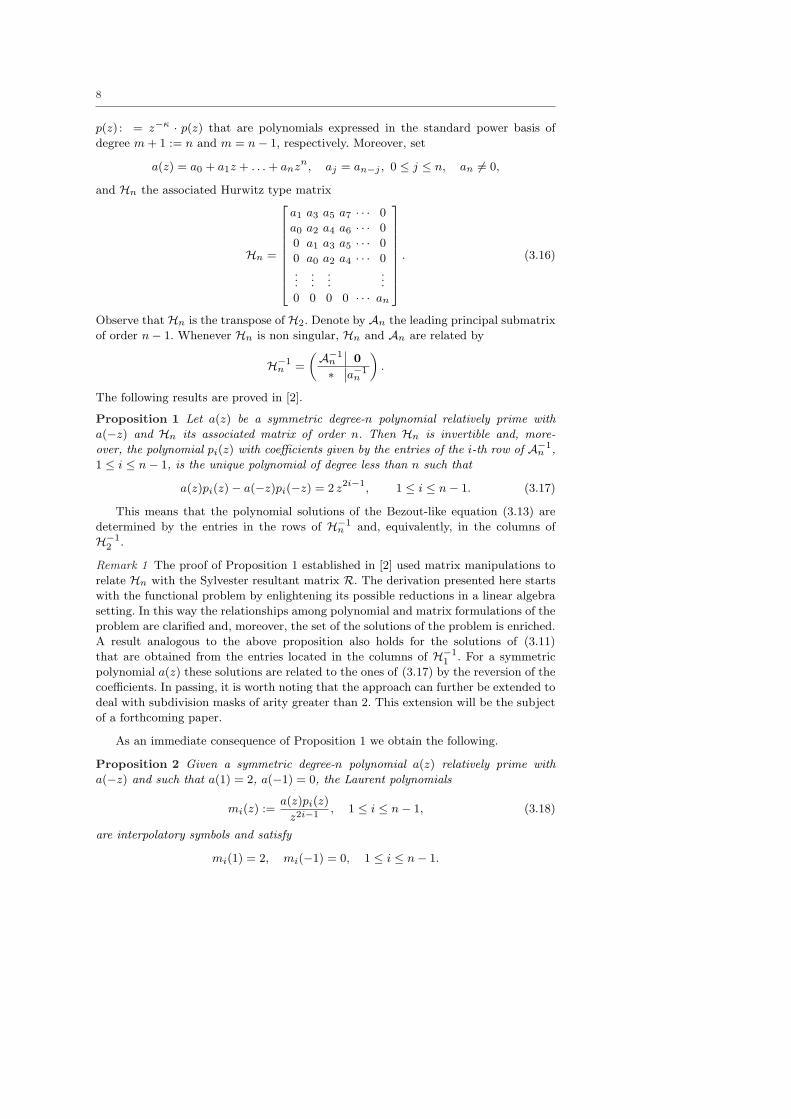
p(z) : = z−κ · p(z) that are polynomials expressed in the standard power basis of

degree m + 1 := n and m = n− 1, respectively. Moreover, set

a(z) = a0 + a1z + . . . + anzn, aj = an−j , 0 ≤ j ≤ n, an 6= 0,

and Hn the associated Hurwitz type matrix

Hn =

a1 a3 a5 a7 · · · 0

a0 a2 a4 a6 · · · 0

0 a1 a3 a5 · · · 0

0 a0 a2 a4 · · · 0...

......

...

0 0 0 0 · · · an

. (3.16)

Observe that Hn is the transpose of H2. Denote by An the leading principal submatrix

of order n− 1. Whenever Hn is non singular, Hn and An are related by

H−1n =

(A−1n 0

∗ a−1n

).

The following results are proved in [2].

Proposition 1 Let a(z) be a symmetric degree-n polynomial relatively prime with

a(−z) and Hn its associated matrix of order n. Then Hn is invertible and, more-

over, the polynomial pi(z) with coefficients given by the entries of the i-th row of A−1n ,

1 ≤ i ≤ n− 1, is the unique polynomial of degree less than n such that

a(z)pi(z)− a(−z)pi(−z) = 2 z2i−1, 1 ≤ i ≤ n− 1. (3.17)

This means that the polynomial solutions of the Bezout-like equation (3.13) are

determined by the entries in the rows of H−1n and, equivalently, in the columns of

H−12 .

Remark 1 The proof of Proposition 1 established in [2] used matrix manipulations to

relate Hn with the Sylvester resultant matrix R. The derivation presented here starts

with the functional problem by enlightening its possible reductions in a linear algebra

setting. In this way the relationships among polynomial and matrix formulations of the

problem are clarified and, moreover, the set of the solutions of the problem is enriched.

A result analogous to the above proposition also holds for the solutions of (3.11)

that are obtained from the entries located in the columns of H−11 . For a symmetric

polynomial a(z) these solutions are related to the ones of (3.17) by the reversion of the

coefficients. In passing, it is worth noting that the approach can further be extended to

deal with subdivision masks of arity greater than 2. This extension will be the subject

of a forthcoming paper.

As an immediate consequence of Proposition 1 we obtain the following.

Proposition 2 Given a symmetric degree-n polynomial a(z) relatively prime with

a(−z) and such that a(1) = 2, a(−1) = 0, the Laurent polynomials

mi(z) :=a(z)pi(z)

z2i−1, 1 ≤ i ≤ n− 1, (3.18)

are interpolatory symbols and satisfy

mi(1) = 2, mi(−1) = 0, 1 ≤ i ≤ n− 1.

9

The result provides a practical way to construct a family of interpolatory masks

from a given approximating one consisting in computing the matrix A−1n and read-

ing its entries. This approach seems to be especially tailored for symmetric Hurwitz

subdivision symbols which result into totally positive (TP) Hurwitz matrices. The pro-

cedures described in [10] can be adjusted for the efficient and stable computations of

the coefficients of the interpolatory masks generated in the B-spline case and “shifted”

affine combinations of them. Different solution methods can rely upon the equivalent

polynomial formulations (3.11), (3.12) and (3.13). Although these latter methods can

perform poorly in a numerical environment, they have at least two advantages for ap-

plications in a numeric-symbolic environment. First, in several interesting cases they

yield semi-explicit representations of the associated interpolatory symbols which can

be useful for the convergence analysis. Secondly, these polynomial methods are par-

ticularly suited to exploit additional features of the symbol a(z). In the next section

we present two computational procedures for solving (3.17) and its variations (3.11),

(3.12) and (3.13) that are effective in contexts of applicative value.

4 Polynomial equation solvers

The condition a(−1) = 0 implies that a(z) = (z + 1)κ · a(z), κ ≥ 1. Effective computa-

tional procedures for computing the interpolatory masks associated with the symmetric

polynomial a(z) of degree n can be developed in two important situations. The first

one is the case where n − κ is very small compared with n, which covers many gene-

ralizations of B-splines. In the second interesting case the value of κ can be small but

the knowledge of the zeros of a(z) permits the representation of the symbol in factored

form. This is the case treated in Definition 1. In the next two subsections we describe

computational methods for dealing with these two cases. Specifically, in Subsection 4.1

we address the first case by representing a(z) in a convenient polynomial basis and then

computing the coefficients of the solution pi(z) represented in such basis. The resulting

algorithm is described in [2]. The case of factored symbols is the subject of Subsection

4.2 where a novel polynomial solver is designed which is based on the partial fraction

decomposition ofpi(z)

a(−z).

4.1 Polynomial equation solver for symbols in Bernstein-type polynomial bases

Let us consider the task of solving a polynomial equation of the more general form

a(z)p(−z) + a(−z)p(z) = b(z), (4.19)

with

deg(a(z)), deg(p(z)) ≤ n, deg(b(z)) ≤ 2n, b(z) = b(−z). (4.20)

The solution method we propose in [2] relies upon the representation of the polynomials

in (4.19) by using the Bernstein type polynomial basis

(1− z)n, (1− z)n−1(1 + z), . . . , (1− z)(1 + z)n−1, (1 + z)n

10

of the vector space of real polynomials of degree less than or equal to n. That is,

a(z) =

n∑

j=0

aj(1− z)n−j(1 + z)j , p(z) =

n∑

j=0

pj(1− z)n−j(1 + z)j .

Moreover let us assume that b(z) is also suitably represented by using the polynomial

basis (1−z)2n, (1−z)2n−1(1+z), . . . , (1−z)(1+z)2n−1, (1+z)2n of the vector space

of real polynomials of degree less than or equal to 2n, namely

b(z) =

2n∑

j=0

bj(1− z)2n−j(1 + z)j .

The Moebius transformation z → w =1 + z

1− zis employed to transform the polynomial

equation (4.19) in the equivalent form

a(w)p

(1

w

)+ a

(1

w

)p(w) = b(w) + b

(1

w

), (4.21)

where

a(w) :=

n∑

j=0

ajwj , p(w) :=

n∑

j=0

pjwj ,

and

b(w) :=bn

2+

n∑

j=1

bn+jwj .

The equation (4.21) reduces to a Toeplitz–plus–Hankel linear system whose coefficient

matrix of order n + 1 is the Toeplitz–plus–Hankel matrix given by

J (a0, . . . , an) =

a0 . . . . . . an

. . ....

. . ....

a0

+

a0 . . . . . . an

......

......

an

.

Under the assumption that a(z) and a(−z) are relatively prime the matrix J turns out

to be invertible [4] and, therefore, the computation of the coefficients of p(w) amounts

to compute the coefficients of b(w) forming the known vector and then to solve the

corresponding linear system. The case b(z) = 2z2s, 1 ≤ s ≤ n, is considered in the

following proposition essentially given in [2].

Proposition 3 Let a(z) =

n∑

j=0

aj(1− z)n−j(1 + z)j , be a symmetric polynomial of

degree n with a(z) and a(−z) relatively prime. Then, the unique polynomial solution

pi(z) of (3.17) satisfies

zpi(z) = (1 + z)npi(1

w), pi(w) :=

n∑

j=0

p(i)j wj , w =

1 + z

1− z,

11

where the coefficients p(i)j of pi(w) are the entries of the solution of the linear system

J (a0, . . . , an)[p(i)0 , . . . , p

(i)n

]T= 21−2n

[ρ(i)n , . . . , ρ

(i)2n

]T,

with

ρ(i)s =

2i∑

j=2i−2n+s

(−1)j(

2i

j

)(2n− 2i

s− j

), n ≤ s ≤ 2n. (4.22)

The computational interest of this result stems from the observation that for

symbols obtained as generalization of the one of B-splines the representation in the

Bernstein-type polynomial basis is extremely sparse and, moreover, in many impor-

tant cases the resulting matrix J (a0, . . . , an) has some special structure so that it can

be explicitly inverted. In this way we are able to find explicit representations of the

polynomial solutions of (3.17). Applications of these techniques are given in Section 6.

4.2 A root-based polynomial equation solver

A different strategy for solving (3.17) can be pursued whenever the factorization of the

symbol is assumed to be known. To be specific, let us suppose that

a(z) = a0 + a1z + . . . + anzn = an

m∏

j=0

(z − zj)kj ,

with zi 6= zj if i 6= j and k0 + . . . + km = n. Then it is shown that the unique solution

pi(z) of (3.17) can be obtained by imposing certain interpolation conditions at the

zeros of a(z) and a(−z).

Let us start by recalling the concept of Hermite-Lagrange interpolation polynomial

of a given differentiable function f(z) on the set of nodes η0, . . . , η` with multiplicities

h0, . . . , h`, h0 + . . .+h` = r +1, respectively. Suppose that the function f(z) possesses

derivatives f (j)(ηi), 0 ≤ j ≤ hi − 1, 0 ≤ i ≤ `. Then there exists a unique polynomial

Hf (z) of degree at most r satisfying the interpolation conditions

H(j)f (ηi) = f (j)(ηi), 0 ≤ j ≤ hi − 1, 0 ≤ i ≤ `.

This polynomial is generally referred to as the Hermite-Lagrange interpolation polyno-

mial of f(z) on the prescribed set of nodes. By setting ω(z) := (z− η0)h0 · · · (z− η`)

h`

we find the Lagrange-type representation

Hf (z) =∑

i=0

hi−1∑

j=0

hi−j−1∑

h=0

f (j)(ηi)1

h!j!

((z − ηi)

hi

ω(z)

)(h)

z=ηi

ω(z)

(z − ηi)hi−j−h

and, equivalently, the partial-fraction representation

Hf (z) = ω(z)∑

i=0

hi∑

s=1

1

(z − ηi)s

hi−s∑

j=0

S(hi − j − s, j, i)

,

where

S(h, j, i) = f (j)(ηi)1

h!j!

((z − ηi)

hi

ω(z)

)(h)

z=ηi

, 0 ≤ h, j ≤ hi − 1, 0 ≤ i ≤ `. (4.23)

12

Let ` = 2m + 1 and η0 = z0, . . . , η(`−1)/2 = zm, η(`+1)/2 = −z0, . . . , η` = −zm with

multiplicities h0 = h(`+1)/2 = k0, . . . , h` = h(`−1)/2 = km. Observe that

r + 1 = h0 + . . . + h` = 2k0 + . . . + 2km = 2n

and

ω(z) =

m∏

i=0

(z − zi)ki

m∏

i=0

(z + zi)ki = a−2

n (−1)na(z)a(−z).

Moreover, let f(z) = 2z2t−1 for a given fixed integer t with 1 ≤ t ≤ n. By replacing

f(z) with its Hermite-Lagrange form in (3.17) we find that

(−1)na2n

(pt(z)

a(−z)− pt(−z)

a(z)

)=

∑

i=0

hi∑

s=1

1

(z − ηi)s

hi−s∑

j=0

S(hi − j − s, j, i)

.

Since a(z) and a(−z) are relatively prime we can separate the partial fraction decom-

positions of the two rational functions on the left–hand side. This gives

(−1)n+1a2n

pt(−z)

a(z)=

m∑

i=0

ki∑

s=1

1

(z − zi)s

ki−s∑

j=0

S(ki − j − s, j, i)

,

and, therefore,

pt(−z) = (−1)n+1a−1n

m∏

j=0

(z − zj)kj

m∑

i=0

ki∑

s=1

1

(z − zi)s

ki−s∑

j=0

S(ki − j − s, j, i)

and

pt(z) = −a−1n

m∏

j=0

(z + zj)kj

m∑

i=0

ki∑

s=1

(−1)s

(z + zi)s

ki−s∑

j=0

S(ki − j − s, j, i)

. (4.24)

Summing up we arrive at the following

Proposition 4 Let a(z) = an∏m

j=0(z − zj)kj be a polynomial of degree n, where

zi 6= zj if i 6= j, k0 + . . . + km = n and a(z) and a(−z) are relatively prime. Then, the

unique polynomial solution pt(z), 1 ≤ t ≤ n, of (3.17) satisfies (4.24) with

S(h, j, i) = f (j)(ηi)1

h!j!

((z − zi)

ki

ω(z)

)(h)

z=zi

, 0 ≤ h, j ≤ ki − 1, 0 ≤ i ≤ m,

where f(z) = 2z2t−1 and ω(z) is the monic polynomial associated with a(z)a(−z).

From a computationally viewpoint the computation of this form of p(z) essentially

reduces to evaluating the coefficients S(h, j, i) defined in (4.23). The derivatives of

wi(z) =(z − ηi)

ki

ω(z)evaluated at z = ηi = zi can be obtained iteratively by successive

differentiations of the relation wi(z) · γi(z) = 1, where γi(z) is the reciprocal of wi(z),

namely,

γi(z) :=

m∏

j=0,j 6=i

(z − zj)kj

m∏

j=0

(z + zj)kj .

The process involves the derivatives of γi(z) at z = ηi = zi which are determined from

those of a(z) · a(−z) obtained by using the Ruffini-Horner scheme.

13

5 An algorithm for deriving non-stationary interpolatory subdivision

schemes

So far we have introduced a quite general strategy for computing a family of non-

stationary interpolatory subdivision schemes associated with a non-stationary approx-

imating subdivision scheme via the solution of equations (3.17) at each recursion step.

The basic procedure turns out to be as follows: Assuming {ak(z), k ≥ 0} are the

symmetric degree-n(k) symbols of an approximating non-stationary scheme with ak(z)

and ak(−z) relatively prime for all k ≥ 0, we construct the non-stationary interpola-

tory subdivision scheme based on the symbols {mki(k)(z), k ≥ 0} where, for each k,

mki(k)(z), 1 ≤ i(k) ≤ n(k) − 1, is one of the interpolatory symbols satisfying (3.17).

Certainly, the performance of the non-stationary subdivision scheme will depend on

the selection of the sequence i(k), k ≥ 0. For clarity we describe the procedure in

algorithmic form.

Appint Algorithm

Input: {ak(z), k ≥ 0}, symmetric degree-n(k) symbols;

{i(k), k ≥ 0}, with 1 ≤ i(k) ≤ n(k)− 1

For k = 0, 1, . . .

Check whether ak(z) is relatively prime with ak(−z)

From ak construct the matrix An(k)

Determine A−1n(k)

(i(k), : ), the i(k)− th row of A−1n(k)

Set pki(k): = A−1

n(k)(i(k), : )

Construct the interpolatory symbol mki(k)(z):=

ak(z)pki(k)(z)

z2 i(k)−1

Output: {mki(k)(z), k ≥ 0}

The computation of A−1n(k)

can be performed by matrix inversion methods applied

to H−1n(k)

or, in the view of the polynomial reductions shown in the previous sections,

by polynomial methods applied for the solution of (3.17). For the non-stationary sub-

division scheme generated by masks mki (z), 1 ≤ i ≤ n(k)− 1, k ≥ 0, we can prove an

important reproduction property: The function space reproduced by the interpolatory

schemes is the same reproduced by the approximating one, at least for all relevant

approximating schemes. First we need a preliminary result given in [6].

Proposition 5 Let {qk(z), k ≥ 0} a sequence of interpolatory symbols. The subdivi-

sion scheme associated with such a sequence reproduces VT,γ if and only if for each

k ≥ 0

qk(e− θ`

2k+1 ) = 2, qk(−e− θ`

2k+1 ) = 0, ` = 1, · · · , N

dh`

dzh`qk(±e

− θ`2k+1 ) = 0, h` = 1, · · · , τ` − 1, ` = 1, · · · , N.

(5.25)

We are now in a position to state the reproduction result.

14

Proposition 6 Let akn(z), k ≥ 0, symmetric symbols of the form

akn(z) = 2

N∏

`=1

τ`−1∏

h`=0

eθ`

2k+1 z + 1

eθ`

2k+1 + 1, k ≥ 0, with ak

n(z), akn(−z) relatively prime.

(5.26)

If the non-stationary subdivision scheme based on the symbols {akn(z), k ≥ 0} is con-

vergent, the interpolatory subdivision scheme based on the symbols

mki (z) =

akn(z)pk

i (z)

z2i−1, 1 ≤ i ≤ T − 1,

whenever convergent, reproduces functions from the space

VT,γ = Span{xh`eθ` x, h` = 0, · · · , τ` − 1, ` = 1, · · · , N}, with T =

N∑

`=1

τ`.

Proof: Due to the special form of the polynomials akn(z), explicitly given in (5.26), it

results

akn(−e

− θ`2k+1 ) = 0,

dh`

dzh`ak

n(−e− θ`

2k+1 ) = 0, h` = 1, · · · , τ` − 1, ` = 1, · · · , N.

By the Leibnitz’s differentiation rule, we easily get an analogous relation to be satisfied

by all mki (z) that is

mki (−e

− θ`2k+1 ) = 0,

dh`

dzh`mk

i (−e− θ`

2k+1 ) = 0, h` = 1, · · · , τ` − 1, ` = 1, · · · , N.

It remains to consider the behavior of mki (z) and its derivatives at the points e

− θ`2k+1 .

Now, since for each k

mki (z) + mk

i (−z) = 2, 1 ≤ i ≤ T − 1,

it follows that

mki (e

− θ`2k+1 ) = 2

as well as

dh`

dzh`mk

i (e− θ`

2k+1 ) = (−1)h`+1 dh`

dzh`mk

i (−e− θ`

2k+1 ) = 0, h` = 1, · · · , τ`−1, ` = 1, · · · , N.

The use of Proposition 5 concludes the proof. ¤

Examples of interpolatory subdivision schemes generated by the Appint Algorithm

and their properties will be investigated in the next sections.

15

6 The interpolatory non-stationary B-spline case and its “generalizations”

This section is devoted to the application of the Appint Algorithm to non-stationary B-

spline subdivision schemes and their generalizations, i.e. symbols being “shifted” affine

combinations of B-spline symbols. In these cases, at each iteration, the solution of the

polynomial equation can be addressed by using the techniques discussed in subsection

4.1 and this leads to an efficient procedure for the computation of the coefficients of

the corresponding family of interpolatory masks. A non-stationary B-spline subdivision

scheme is associated to {ak(z), k ≥ 0}, the set of degree-k symmetric polynomials

ak(z) =(1 + z)k

2k−1trivially relatively prime with ak(−z) =

(1− z)k

2k−1. Thus, equation

(3.17) reads as

(1 + z)k(zpki (z)) + (1− z)k(−zpk

i (−z)) = 2kz2i, 1 ≤ i ≤ k − 1, (6.27)

which gives us a simple way to compute the coefficients of the polynomial pki (z). For

the sake of simplicity we refer to the polynomial −zpki (−z) as to pk(z). Since ak(z) =

(1 + z)k

2k−1we find that ak(w) :=

wk

2k−1, the matrix J (a0, . . . , an) is antidiagonal and,

therefore, the solution pk(w) of (4.21) can immediately be reconstructed from the

coefficients of bk(w) in Proposition 3. Indeed, we obtain that

wk ∑kj=0 pjw

−j + 1wk

∑kj=0 pjw

j =

2−k(ρ(i)0 w−k + . . . + ρ

(i)k−1w−1 + ρ

(i)k + ρ

(i)k+1w + . . . + ρ

(i)2k wk

) (6.28)

which gives

pj = 2−kρ(i)j , 0 ≤ j ≤ k − 1, pk = 2−k−1ρ

(i)k . (6.29)

As a generalization of the previous situation we can consider a five term “shifted” affine

combination of a B-spline symbol, i.e. we consider the symbol

ckn(z) =

(1 + z)n−4

2n−5

(αk + βkz + (1− 2αk − 2βk)z2 + βkz3 + αkz4

), (6.30)

with bk(z) :=(αk + βkz + (1− 2αk − 2βk)z2 + βkz3 + αkz4

)and bk(−z) relatively

prime for all k. As shown in [3], this symbol allows us to get a unified representation of

several of the well known (stationary and non-stationary) subdivision schemes corre-

sponding to specific settings of the combination parameters αk, βk ∈ R and to different

values of n ∈ N, n > 4. For example, we can range from degree-(n−5) to degree-(n−1)

B-splines. In fact, when αk = βk = 0, ckn(z) coincides exactly with the symbol of the

degree-(n − 5) B-spline, while for αk = 0, βk = 14 and αk = 1

16 , βk = 14 we have

the degree-(n − 3) and degree-(n − 1) B-splines, respectively. In view of (6.27), it is

convenient to write the quartic polynomial bk(z), as

1

16

((1− 4βk)(1− z)4 + (16αk + 4βk − 2)(1− z)2(1 + z)2 + (1 + z)4

),

and derive the polynomial ak(w) = akn−4wn−4 + ak

n−2wn−2 + aknwn in (6.27) explicitly

as

ak(w) =1− 4βk

16wn−4 16αk + 4βk − 2

16wn−2 +

1

16wn.

16

The above expression of a(w) allows us to provide an efficient strategy for the compu-

tation of p(w) =∑n

j=0 pjwj which reduces to the solution of a 5 × 5 linear system.

In fact, we can observe that in this case the matrix J (a0, . . . , an) is upper triangular

(with respect to to the main antidiagonal) except that for a bulge of order 5 in the

up–right corner. A direct comparison of the polynomial coefficients in the left hand

side of (6.27), i.e.,

(ak

n−4wn−4 + akn−2wn−2 + ak

nwn) (

p0 + · · ·+ pnw−n)+

(ak

n−4w−n+4 + akn−2w−n+2 + ak

nw−n)

(p0 + · · ·+ pnwn) ,

with those in the right hand side of (6.27), i.e.,

(ρ(i)0 w−n + . . . + ρ

(i)n−1w−1 + ρ

(i)n + ρ

(i)n+1w + . . . + ρ

(i)2nwn),

leads to the following relations for the coefficients

anp0 = 24−nρ(i)0 ,

anp1 = 24−nρ(i)1 ,

anp2 = 24−nρ(i)2 − an−2p0,

anp3 = 24−nρ(i)3 − an−2p1,

anpj = 24−nρ(i)j + an−4pj−4 − an−2pj−2, j = 4, · · ·n− 5,

(6.31)

and the linear system

anpn−4 + an−4pn = 24−nρ(i)n−4 − an−2pn−6 − an−4pn−8

anpn−3 + an−4pn−1 = 24−nρ(i)n−3 − an−2pn−5 − an−4pn−7

(an + an−4) pn−2 + an−2pn−4 + an−2pn = 24−nρ(i)n−2 − an−4pn−6

(an + an−2) pn−1 + (an−2 + an−4) pn−3 = 24−nρ(i)n−1 − an−4pn−5

2an−4pn−4 + 2an−2pn−2 + 2anpn = 23−nρ(i)n ,

to be solved for getting the remaining coefficients.

A further generalization of the B-spline case is given by the non-stationary affine

combination (as in (6.30)) of exponential reproducing spline symbols defined in (2.5).

This generalization will be considered in several examples in the next section.

17

7 Interpolatory exponential reproducing non-stationary subdivision

schemes

In the following we consider several examples of non-stationary subdivision symbols

depending on a parameter vk ∈ (0, +∞), k ≥ 0, defined through the expression

vk =1

2(eθ/2k+1

+ e−θ/2k+1)

with θ = θ`, ` = 1, ..., N , as in Lemma 1. As shown in [1] this means that, once

assigned the starting value v−1 ∈ (−1, +∞), the parameter vk can be recursively up-

dated at each successive iteration through the formula vk =√

vk−1+12 , k ≥ 0. For

each non-stationary subdivision scheme associated to these symbols we construct the

corresponding family of interpolatory symbols maintaining the same reproduction prop-

erties. The interpolatory schemes can be obtained directly by inverting the subdivision

matrix or, differently, by using the strategy discussed in subsection 4.2.

Example 1: We consider the C2 approximating scheme by Morin et al. [9] whose

k-level symbol is

ak3(z) =

1

2(z + 1)2

z2 + 2vkz + 1

2(vk + 1)

and the related mask

ak3 =

[1

4(1 + vk)

1

2

1 + 2vk

2(1 + vk)

1

2

1

4(1 + vk)

].

Since the polynomials ak3(z), ak

3(−z) are relatively prime, we can apply the AppintAlgorithm involving at each step the matrix

Ak3 =

1

2

1 1 0

12(1+vk)

1+2vk

1+vk1

2(1+vk)

0 1 1

from which we obtain the following inverse

(Ak3 )−1

=1

2vk

4vk + 1 −2(1 + vk) 1

−1 2(1 + vk) −1

1 −2(1 + vk) 4vk + 1

.

The rows of (Ak3)−1 define three interpolatory subdivision masks

mk3,1 =

[1+4vk

8vk(vk+1)1

12(vk)2+4vk−18vk(vk+1)

0 − 4(vk)2+18vk(vk+1)

0 18vk(vk+1)

],

mk3,2 =

[− 1

8vk(vk+1)0

(2vk+1)2

8vk(vk+1)1

(2vk+1)2

8vk(vk+1)0 − 1

8vk(vk+1)

],

mk3,3 =

[1

8vk(vk+1)0 − 4(vk)2+1

8vk(vk+1)0

12(vk)2+4vk−18vk(vk+1)

1 1+4vk

8vk(vk+1)

](7.32)

18

associated with the symbols

mk3,1(z) = 4vk+1

2vk ak3(z)− vk+1

vk zak3(z) + 1

2vk z2ak3(z),

mk3,2(z) = − 1

2vk ak3(z) + vk+1

vk zak3(z)− 1

2vk z2ak3(z),

mk3,3(z) = 1

2vk ak3(z)− vk+1

vk zak3(z) + 4vk+1

2vk z2ak3(z).

(7.33)

Notice that the interpolatory masks {mk3,2, k ≥ 0} corresponds to the C1 four-point

scheme introduced in [1], which possesses the special feature of reproducing functions

from the space 〈1, x, eθx, e−θx〉 for any non-negative real or imaginary constant θ,

as well as the approximating non-stationary subdivision scheme correspondent to the

masks {ak3 , k ≥ 0}. More precisely, whenever we apply this interpolatory subdivision

mask to an initial polyline made of points lying equidistant with uniform parameter

spacing u > 0 on a given curve from that function space, by setting

v−1 =1

2(eθu + e−θu) (7.34)

we are able to reproduce the curve from which those points are sampled. Fundamental

shapes in CAGD that turn out to be reproducible by this subdivision scheme are all

conic sections (Figure 1).

(a) (b) (c)

Fig. 1 Exact reconstruction of conic sections through the interpolating scheme with masks{mk

3,2, k ≥ 0}. Dashed lines depict the assumed starting polygons. The corresponding initial

parameter is respectively chosen as (a) v−1 = 1, (b) v−1 = 12, (c) v−1 = cosh

(35

).

Observe that the pictures in Figure 1 correspond also to a reproduction capability of

the subdivision schemes discussed in the sequel.

In order to derive the interpolatory symbols associated to {ak3(z), k ≥ 0}, one can

alternatively employ the techniques introduced in subsection 4.2 based on the compu-

tation of the partial fraction decompositions of certain rational functions associated

with the given symbol. For instance, we find

2z3

ak3(z)ak

3(−z)=

2(vk + 1)

(vk − 1)(z + 1)2− 2(vk + 1)

(vk − 1)(z − 1)2

+2(vk + 1)

vk(vk − 1)(z2 − 2vkz + 1)− 2(vk + 1)

vk(vk − 1)(z2 + 2vkz + 1)

19

which gives

pk2(−z)

ak3(z)

=2(vk + 1)

vk(vk − 1)(z2 + 2vkz + 1)− 2(vk + 1)

(vk − 1)(z + 1)2

and, hence,

pk2(z) =

(1− z)2

2vk(vk − 1)− z2 − 2vkz + 1

2(vk − 1)=

1

2vk

(−z2 + 2(vk + 1)z − 1

).

Observe that the coefficients of pk2(z) are the entries in the second row of (Ak

3)−1.

Example 2: Let

ak5,1(z) =

(z + 1)4(z2 + 2vkz + 1)

16(vk + 1)

be the k-level symbol of the first C4 approximating scheme proposed in [11] and

ak5,1 =

1

16(vk + 1)

[1 2(vk + 2) 8vk + 7 4(3vk + 2) 8vk + 7 2(vk + 2) 1

]

the associated mask. Since, again, ak5,1(z) and ak

5,1(−z) are relatively prime, running

the Appint Algorithm, at each step we construct the matrix

Ak5,1 =

1

16(vk + 1)

2(vk + 2) 4(3vk + 2) 2(vk + 2) 0 0

1 8vk + 7 8vk + 7 1 0

0 2(vk + 2) 4(3vk + 2) 2(vk + 2) 0

0 1 8vk + 7 8vk + 7 1

0 0 2(vk + 2) 4(3vk + 2) 2(vk + 2)

and by taking the rows of its inverse we get the following five interpolatory masks

20

mk5,1,1 =

[32(vk)2+29vk+2

64vk(vk+1)21

(2vk+1)(70(vk)2+41vk−6)64vk(vk+1)2

0−70(vk)3−44(vk)2+7vk+2

32vk(vk+1)2

042(vk)3+20(vk)2−vk+2

32vk(vk+1)20 − (2vk+1)(10(vk)2−vk+6)

64vk(vk+1)20 5vk+2

64vk(vk+1)2

],

mk5,1,2 =

[− 5vk+2

64vk(vk+1)20

20(vk)3+40(vk)2+39vk+664vk(vk+1)2

130(vk)3+60(vk)2+17vk−2

32vk(vk+1)2

0 − 10(vk)3+20(vk)2+3vk+232vk(vk+1)2

0(4(vk)2+3)(vk+2)

64vk(vk+1)20 − vk+2

64vk(vk+1)2

],

mk5,1,3 =

[vk+2

64vk(vk+1)20 − (2vk+3)(2(vk)2+vk+2)

64vk(vk+1)20

(3vk+2)(6(vk)2+8vk+1)32vk(vk+1)2

1(3vk+2)(6(vk)2+8vk+1)

32vk(vk+1)20 − (2vk+3)(2(vk)2+vk+2)

64vk(vk+1)20 vk+2

64vk(vk+1)2

],

mk5,1,4 =

[− vk+2

64vk(vk+1)20

(4(vk)2+3)(vk+2)64vk(vk+1)2

0 − 10(vk)3+20(vk)2+3vk+232vk(vk+1)2

030(vk)3+60(vk)2+17vk−2

32vk(vk+1)21

20(vk)3+40(vk)2+39vk+664vk(vk+1)2

0 − 5vk+264vk(vk+1)2

],

mk5,1,5 =

[5vk+2

64vk(vk+1)20 − (2vk+1)(10(vk)2−vk+6)

64vk(vk+1)20

42(vk)3+20(vk)2−vk+232vk(vk+1)2

0−70(vk)3−44(vk)2+7vk+2

32vk(vk+1)20

(2vk+1)(70(vk)2+41vk−6)64vk(vk+1)2

132(vk)2+29vk+2

64vk(vk+1)2

].

Note that mk5,1,3 defines the mask of the interpolatory six-point scheme proposed in

[11, Section 4.1], whose symbol is

mk5,1,3(z) = vk+2

4vk(vk+1)ak5,1(z)− (vk+2)2

2vk(vk+1)zak

5,1(z) +4(vk)2+9vk+6

2vk(vk+1)z2ak

5,1(z)

− (vk+2)2

2vk(vk+1)z3ak

5,1(z) + vk+24vk(vk+1)

z4ak5,1(z).

Fig. 2 Comparison between limit curves obtained through the interpolatory schemes{mk

3,2, k ≥ 0}, (left) and {mk5,1,3, k ≥ 0}, (right) starting from the same initial value

v−1 = 1.5.

21

Exactly like the non-stationary approximating subdivision scheme correspondent to

{ak5,1(z), k ≥ 0}, such a scheme can reproduce functions in the space

〈1, x, x2, x3, eθx, e−θx〉 for any non-negative real or imaginary constant θ. Hence, it

allows an exact representation of cubics, circles and conic sections (see Figure 1) when

the vertices of the starting polyline are equally spaced samples and the initial parameter

v−1 is chosen as in (7.34). Moreover the limit curves generated by such a scheme are

featured by C2 smoothness for any choice of the starting parameter v−1 ∈ (−1, +∞).

An application example of this subdivision scheme to an arbitrary starting polyline is

given in Figure 2.

Example 3: We continue by considering another C4 approximating scheme proposed

in [11]. Its k-level symbol is of the form

ak5,2(z) =

(z + 1)2(z2 + 2vkz + 1)(z2 + 2(2(vk)2 − 1)z + 1)

16(vk)2(vk + 1)

and the associated mask is

ak5,2 =

1

16(vk)2(vk + 1)

[1 2vk(2vk + 1) 8(vk)3 + 8(vk)2 − 1 4vk(4(vk)2 + 2vk − 1)

8(vk)3 + 8(vk)2 − 1 2vk(2vk + 1) 1]

.

Now being ak5,2(z) and ak

5,2(−z) relatively prime, we can apply the Appint Algo-

rithm where the matrix to be inverted, besides a factor 116(vk)2(vk+1)

, reads as

Ak5,2 =

4(vk)2 + 2vk 16(vk)3 + 8(vk)2 − 4vk 4(vk)2 + 2vk 0 0

1 8(vk)3 + 8(vk)2 − 1 8(vk)3 + 8(vk)2 − 1 1 0

0 4(vk)2 + 2vk 16(vk)3 + 8(vk)2 − 4vk 4(vk)2 + 2vk 0

0 1 8(vk)3 + 8(vk)2 − 1 8(vk)3 + 8(vk)2 − 1 1

0 0 4(vk)2 + 2vk 16(vk)3 + 8(vk)2 − 4vk 4(vk)2 + 2vk

.

The 5 interpolatory masks built upon the rows of its inverse are

22

mk5,2,1 =

[(2vk+1)(32(vk)4+16(vk)3−24(vk)2−8vk+5)

64(vk)2(2vk−1)(2(vk)2−1)(vk+1)21

(2vk+1)(4(vk)2+2vk−1)(64(vk)5−48(vk)3−4(vk)2+6vk+3)64(vk)2(2vk−1)(2(vk)2−1)(vk+1)2

0 − (4(vk)2+2vk−1)(32(vk)3+12(vk)2−18vk−5)32(vk)2(vk+1)2

0(2vk+1)(64(vk)5−16(vk)4−48(vk)3+20(vk)2+4vk−3)

32(vk)2(2vk−1)(vk+1)2

0 − (2vk+1)(4(vk)2+2vk−1)(16(vk)3−12(vk)2−6vk+5)64(vk)2(2vk−1)(2(vk)2−1)(vk+1)2

0 4vk+364(vk)2(2(vk)2−1)(vk+1)2

],

mk5,2,2 =

[− 4vk+3

64(vk)2(2(vk)2−1)(vk+1)20

(2vk+1)(4(vk)2+2vk−1)(16(vk)3−4(vk)2−6vk+1)(64(vk)2(vk+1)2(2vk−1)(2(vk)2−1))

1

(2vk+1)(4(vk)2+2vk−1)(12(vk)2−2vk−3)32(vk)2(2vk−1)(vk+1)2

0 − (4(vk)2+2vk−1)(4(vk)2+2vk+1)32(vk)2(vk+1)2

0(2vk+1)(16(vk)4−12(vk)2+3)

64(vk)2(2vk−1)(2(vk)2−1)(vk+1)20 − 2vk+1

16(vk)2(8vk−4)(2(vk)2−1)(vk+1)2

],

mk5,2,3 =

[2vk+1

64(vk)2(2vk−1)(2(vk)2−1)(vk+1)20 − (4(vk)2+2vk−1)2

64(vk)2(2(vk)2−1)(vk+1)20

(2vk+1)(4(vk)2+2vk−1)2

32(vk)2(2vk−1)(vk+1)21

(2vk+1)(4(vk)2+2vk−1)2

32(vk)2(2vk−1)(vk+1)2

0 − (4(vk)2+2vk−1)2

64(vk)2(2(vk)2−1)(vk+1)20 2vk+1

64(vk)2(2vk−1)(2(vk)2−1)(vk+1)2

],

mk5,2,4 =

[− 2vk+1

64(vk)2(2vk−1)(2(vk)2−1)(vk+1)20

(2vk+1)(16(vk)4−12(vk)2+3)64(vk)2(2vk−1)(2(vk)2−1)(vk+1)2

0

− (4(vk)2+2vk−1)(4(vk)2+2vk+1)32(vk)2(vk+1)2

0(2vk+1)(4(vk)2+2vk−1)(12(vk)2−2vk−3)

32(vk)2(2vk−1)(vk+1)2

1(2vk+1)(4(vk)2+2vk−1)(16(vk)3−4(vk)2−6vk+1)

64(vk)2(vk+1)2(2vk−1)(2(vk)2−1)0 − 4vk+3

64(vk)2(2(vk)2−1)(vk+1)2

],

mk5,2,5 =

[4vk+3

64(vk)2(2(vk)2−1)(vk+1)20 − (2vk+1)(4(vk)2+2vk−1)(16(vk)3−12(vk)2−6vk+5)

64(vk)2(2vk−1)(2(vk)2−1)(vk+1)20

(2vk+1)(64(vk)5−16(vk)4−48(vk)3+20(vk)2+4vk−3)32(vk)2(2vk−1)(vk+1)2

0 − (4(vk)2+2vk−1)(32(vk)3+12(vk)2−18vk−5)32(vk)2(vk+1)2

0

(2vk+1)(4(vk)2+2vk−1)(64(vk)5−48(vk)3−4(vk)2+6vk+3)64(vk)2(2vk−1)(2(vk)2−1)(vk+1)2

1(2vk+1)(32(vk)4+16(vk)3−24(vk)2−8vk+5)

64(vk)2(2vk−1)(2(vk)2−1)(vk+1)2

].

Note that {mk5,2,3, k ≥ 0}, defines the C2 interpolatory six-point scheme presented in

[11, Section 4.2]. Such a scheme is featured by the capability of reproducing functions

in the space 〈1, x, eθx, e−θx, e2θx, e−2θx〉 for any non-negative real or imaginary

constant θ, exactly as it happens for the corresponding non-stationary approximating

scheme {ak5,2, k ≥ 0}. Hence, it allows an exact representation of algebraic curves

of the second order (i.e. described by means of parametric equations involving order-

2 trigonometric functions) such as the cardioid, Pascal’s limacon, ... (see Figure 3)

whenever the starting parameter v−1 is defined according to (7.34).

Example 4: We conclude by showing that the C4 approximating scheme with k-level

symbol

ak5,3(z) =

(z + 1)2(z2 + 2vkz + 1)2

8(vk + 1)2

and mask

ak5,3 =

1

8(vk + 1)2

[1 2(2vk + 1) 4(vk)2 + 8vk + 3 4(2(vk)2 + 2vk + 1)

4(vk)2 + 8vk + 3 2(2vk + 1) 1]

,

23

(a) (b) (c)

(d) (e) (f)

Fig. 3 Exact reconstruction of the cardioid (a), the deltoid (b), the lemniscate of Gerono (c),Pascal’s limacon (d), the piriform (e) and the eight curve (f) through the interpolating scheme{mk

5,2,3, k ≥ 0}, with starting parameter v−1 = 12. Dashed lines denote the chosen starting

polygons made of 6 points sampled at a uniform parameter spacing of π3.

recently proposed in [11], satisfies the property that ak5,3(z) and ak

5,3(−z) are relativelyprime and hence can be transformed into a family of interpolating schemes with thesame reproduction properties. To this purpose we compute the inverse of the associatedmatrix which, besides a factor 1

8(vk+1)2, reads as

Ak5,3 =

2(2vk + 1) 4(2(vk)2 + 2vk + 1) 2(2vk + 1) 0 0

1 4(vk)2 + 8vk + 3 4(vk)2 + 8vk + 3 1 0

0 2(2vk + 1) 4(2(vk)2 + 2vk + 1) 2(2vk + 1) 0

0 1 4(vk)2 + 8vk + 3 4(vk)2 + 8vk + 3 1

0 0 2(2vk + 1) 4(2(vk)2 + 2vk + 1) 2(2vk + 1)

and apply the Appint Algorithm. The 5 interpolatory masks that we obtain are

24

mk5,3,1 =

[(2vk+1)(8(vk)3+12(vk)2+1)

64(vk)3(vk+1)21

(2vk+1)(32(vk)5+48(vk)4+32(vk)3−8(vk)2+1)64(vk+1)2(vk)3

0

− 64(vk)6+48(vk)5−8(vk)4−8(vk)3+6(vk)2+2vk+132(vk+1)2(vk)3

0(2vk+1)(16(vk)5+4(vk)3+2(vk)2−1)

32(vk+1)2(vk)3

0 − (2vk+1)(16(vk)3−1)64(vk+1)2(vk)3

04(vk)2+2vk+164(vk)3(vk+1)2

],

mk5,3,2 =

[− 4(vk)2+2vk+1

64(vk)3(vk+1)20

(2vk+1)(24(vk)3+12(vk)2−1)64(vk+1)2(vk)3)

1

(2vk+1)(24(vk)4+12(vk)3−2(vk)2+1)32(vk+1)2(vk)3

0 − 16(vk)5+8(vk)4+8(vk)3+6(vk)2−2vk−132(vk+1)2(vk)3

0(2vk+1)(8(vk)2−1)

64(vk+1)2(vk)30 − 2vk+1

64(vk)3(vk+1)2

],

mk5,3,3 =

[2vk+1

64(vk)3(vk+1)20 − (4vk+1)(4(vk)2+2vk−1)

64(vk)3(vk+1)20

(2vk+1)(2(vk)2+2vk+1)(4(vk)2+2vk−1)32(vk)3(vk+1)2

1(2vk+1)(2(vk)2+2vk+1)(4(vk)2+2vk−1)

32(vk)3(vk+1)2

0 − (4vk+1)(4(vk)2+2vk−1)64(vk)3(vk+1)2

0 2vk+164(vk)3(vk+1)2

],

mk5,3,4 =

[− 2vk+1

64(vk)3(vk+1)20

(2vk+1)(8(vk)2−1)64(vk+1)2(vk)3

0

− 16(vk)5+8(vk)4+8(vk)3+6(vk)2−2vk−132(vk+1)2(vk)3

0(2vk+1)(24(vk)4+12(vk)3−2(vk)2+1)

32(vk+1)2(vk)3

1(2vk+1)(24(vk)3+12(vk)2−1)

64(vk+1)2(vk)3)0 − 4(vk)2+2vk+1

64(vk)3(vk+1)2

],

mk5,3,5 =

[4(vk)2+2vk+164(vk)3(vk+1)2

0 − (2vk+1)(16(vk)3−1)64(vk+1)2(vk)3

0

(2vk+1)(16(vk)5+4(vk)3+2(vk)2−1)32(vk+1)2(vk)3

0 − 64(vk)6+48(vk)5−8(vk)4−8(vk)3+6(vk)2+2vk+132(vk+1)2(vk)3

0(2vk+1)(32(vk)5+48(vk)4+32(vk)3−8(vk)2+1)

64(vk+1)2(vk)31

(2vk+1)(8(vk)3+12(vk)2+1)64(vk)3(vk+1)2

].

Note that {mk5,3,3, k ≥ 0}, defines a C2 interpolatory six-point scheme which corre-

sponds to the one presented in [11, Section 4.3]. Like its approximating correspondent

{ak5,3, k ≥ 0}, it is featured by the capability of reproducing functions in the space

〈1, x, eθx, e−θx, xeθx, xe−θx〉 for any non-negative real or imaginary constant θ. It

means that an exact representation of spirals, of great interest in engineering such as

the circle involute which represents the curve employed in most gear-tooth profiles, (see

Figure 4) can be obtained. Like in the previous cases, the reproduction of these curves

is allowed whenever the subdivision process is started from equally spaced samples and

the initial parameter v−1 has been opportunely set as described in (7.34).

8 Conclusions and Future Work

A novel approach based on polynomial and structured matrix technology has been

presented for the computation of a family of interpolatory non-stationary subdivision

25

(a) (b)

Fig. 4 Exact reconstruction of the Archimedean spiral (a) and of the circle involute (b)through the interpolating scheme mk

5,3,3 with starting parameter v−1 = cos(

4π5

). Dashed

lines denote the chosen starting polygons made of 6 points sampled at a uniform parameterspacing of 4π

5.

schemes from a symmetric non-stationary, non-interpolatory one. The approach reduces

the functional problem either to the inversion of certain structured matrices of Hurwitz

or Sylvester resultant form or to the solution of certain Bezout-like polynomial equa-

tions. Efficient computational procedures for both problems have been proposed. It was

shown that the interpolatory schemes are capable of generating the same functional

space as the approximating one. In principle our approach could be extended to more

general approximating schemes of arity p greater than 2. The extension requires to in-

vestigate the structural properties of Sylvester-type resultant matrices for polynomial

sets consisting of more than 2 polynomials. This will be the subject of a forthcoming

paper. A fundamental issue is concerned with the analysis of the convergence properties

of the subdivision schemes generated by our techniques. The semi–explicit representa-

tions of the symbols obtained by solving the polynomial formulation would be useful

to provide some insights on this difficult topic. Finally, the use of parametric symbols

leads to symbolic inversion problems for structured matrices with Hurwitz or Sylvester

resultant form. The adaptation of customary methods to work efficiently in this case

is an ongoing research.

References

1. C. Beccari, G. Casciola, and L. Romani. A non-stationary uniform tension controlledinterpolating 4-point scheme reproducing conics. Comput. Aided Geom. Design, 24(1):1–9, 2007.

2. C. Conti, L. Gemignani, and L. Romani. From symmetric subdivision masks of Hurwitztype to interpolatory subdivision masks. Linear Algebra Appl., 431:1971–1987, 2009.

3. C. Conti and L. Romani. Affine combination of b-spline subdivision masks and its non-stationary counterparts. Submitted, 2009.

4. C. J. Demeure and C. T. Mullis. A Newton-Raphson method for moving-average spectralfactorization using the Euclid algorithm. IEEE Trans. Acoust. Speech Signal Process.,38(10):1697–1709, 1990.

5. N. Dyn and D. Levin. Subdivision schemes in geometric modelling. Acta Numer., 11:73–144, 2002.

6. N. Dyn, D. Levin, and A. Luzzatto. Exponentials reproducing subdivision schemes. Found.Comput. Math., 3(2):187–206, 2003.

26

7. M. Gasca and J. M. Pena. On factorizations of totally positive matrices. In Total positivityand its applications (Jaca, 1994), volume 359 of Math. Appl., pages 109–130. Kluwer Acad.Publ., Dordrecht, 1996.

8. C. A. Micchelli. Interpolatory subdivision schemes and wavelets. J. Approx. Theory,86(1):41–71, 1996.

9. G. Morin, J. Warren, and H. Weimer. A subdivision scheme for surfaces of revolution. Com-put. Aided Geom. Design, 18(5):483–502, 2001. Subdivision algorithms (Schloss Dagstuhl,2000).

10. J. M. Pena. Characterizations and stable tests for the Routh-Hurwitz conditions and fortotal positivity. Linear Algebra Appl., 393:319–332, 2004.

11. L. Romani. From approximating subdivision schemes for exponential splines to high-performance interpolating algorithms. J. Comput. Appl. Math., 224(1):383–396, 2009.

12. L. L. Schumaker. Spline functions: basic theory. Cambridge Mathematical Library. Cam-bridge University Press, Cambridge, third edition, 2007.

13. J. Warren and H. Weimer. Subdivision methods for geometric design: a constructiveapproach. Morgan Kaufmann, 2002.